Numerical Methods of Continuum Mechanics
82
Numerical Methods of Continuum Mechanics Version as of August 24, 2015 Lecture notes by Prof. Dr. Vincent Heuveline Faculty of Mathematics and Computer Science Heidelberg University Summer term 2015
Transcript of Numerical Methods of Continuum Mechanics
Numerical Methods of Continuum Mechanics
Version as of August 24, 2015
Lecture notes
by
Prof. Dr. Vincent Heuveline
Faculty of Mathematics and Computer Science
Heidelberg University
Summer term 2015

3
Contents
1 Introduction 51.1 Examples for fields of applications . . . . . . . . . . . . . . . . . . . . . . . . . 5
1.1.1 Elasticity and plasticity . . . . . . . . . . . . . . . . . . . . . . . . . . . 5
1.1.2 Fluid mechanics . . . . . . . . . . . . . . . . . . . . . . . . . . . . . . . 6
1.1.3 Combination of elasticity/plasticiy and fluid mechanics . . . . . . . . . . 9
1.2 Notation . . . . . . . . . . . . . . . . . . . . . . . . . . . . . . . . . . . . . . . . 10
1.3 Review of Vector Calculus . . . . . . . . . . . . . . . . . . . . . . . . . . . . . . 10
1.4 Path of lecture . . . . . . . . . . . . . . . . . . . . . . . . . . . . . . . . . . . . 12
2 The equation of fluid flow - Introduction to modelling 13
2.1 Lagrangian and Eulerian Systems: Substantial Derivative . . . . . . . . . . . . 13
2.1.1 The Lagrangian viewpoint . . . . . . . . . . . . . . . . . . . . . . . . . . 13
2.1.2 The Eulerian viewpoint . . . . . . . . . . . . . . . . . . . . . . . . . . . 14
2.1.3 The substantial derivative . . . . . . . . . . . . . . . . . . . . . . . . . . 14
2.2 Conservation of mass . . . . . . . . . . . . . . . . . . . . . . . . . . . . . . . . . 15
2.3 Conservation of momentum . . . . . . . . . . . . . . . . . . . . . . . . . . . . . 16
2.3.1 Conservation of angular momentum . . . . . . . . . . . . . . . . . . . . 17
2.3.2 Conservation of energy . . . . . . . . . . . . . . . . . . . . . . . . . . . . 18
2.3.3 Balance equations . . . . . . . . . . . . . . . . . . . . . . . . . . . . . . 20
2.3.4 Kinematic properties . . . . . . . . . . . . . . . . . . . . . . . . . . . . . 20
2.3.5 Material properties . . . . . . . . . . . . . . . . . . . . . . . . . . . . . . 27
3 Approximating Steady Flows 333.1 The Stokes problem: Introduction to Mixed Methods . . . . . . . . . . . . . . . 33
3.2 Formulation and Stability of the Approximation . . . . . . . . . . . . . . . . . . 37
4 Time dependent Navier-Stokes equations 43
5 Saddle-point problem 475.1 General setting . . . . . . . . . . . . . . . . . . . . . . . . . . . . . . . . . . . . 47
5.1.1 Discrete setting . . . . . . . . . . . . . . . . . . . . . . . . . . . . . . . . 48
5.2 The inf − sup condition . . . . . . . . . . . . . . . . . . . . . . . . . . . . . . . 49
5.2.1 The Stokes equations . . . . . . . . . . . . . . . . . . . . . . . . . . . . . 49
5.2.2 Laplace equation . . . . . . . . . . . . . . . . . . . . . . . . . . . . . . . 49
5.2.3 The inf − sup condition . . . . . . . . . . . . . . . . . . . . . . . . . . . 50
6 A posteriori error estimation 55
6.1 Introduction . . . . . . . . . . . . . . . . . . . . . . . . . . . . . . . . . . . . . . 55
6.2 Residual based error estimator . . . . . . . . . . . . . . . . . . . . . . . . . . . 55
6.2.1 Residual estimators . . . . . . . . . . . . . . . . . . . . . . . . . . . . . . 57
6.2.2 Dual weighted Residual method (DWR) . . . . . . . . . . . . . . . . . . 58
6.3 Exact grid optimization . . . . . . . . . . . . . . . . . . . . . . . . . . . . . . . 60

4 Contents
7 Practical aspects 617.1 Solution of the discrete Stokes problems . . . . . . . . . . . . . . . . . . . . . . 61
7.1.1 Schur complement method . . . . . . . . . . . . . . . . . . . . . . . . . . 627.2 Solution of the stationary Navier-Stokes equations . . . . . . . . . . . . . . . . 64
7.2.1 Discretization of the convective terms . . . . . . . . . . . . . . . . . . . 647.2.2 Linearization . . . . . . . . . . . . . . . . . . . . . . . . . . . . . . . . . 717.2.3 Algebraic solution of the linearized problems . . . . . . . . . . . . . . . 72
7.3 Solution of the instationary Navier-Stokes equations . . . . . . . . . . . . . . . 757.3.1 Time-stepping schemes . . . . . . . . . . . . . . . . . . . . . . . . . . . . 757.3.2 Projection methods . . . . . . . . . . . . . . . . . . . . . . . . . . . . . . 77
Bibliography 79
Index 81

5
1 Introduction
Continuum mechanics deals with mechanics of continuous media. The emphasis lies on con-tinuous, which means that the considered media are not understood as a set of point massesas their atomic structure suggests to, but the medium is seen as a continuum. Consequently,observations are described from a macroscopic point of view and not a microscopic one. Thisoffers the possibility to mathematically describe the quantities of interest, for example the ve-locity of the medium or its deformation, as - often continuous or even continuously differentiable- functions and analyse them by means of calculus. This is known as continuum hypothesis.
By modelling the underlying physical principles this approach naturally leads to partial differ-ential equations, whose analytical solution for practically relevant applications cannot be givenin an explicit way. As a consequence, to examine these processes, it is necessary to developadequat numerical methods and to analyse both the methods themself and their results.
First, a short, for sure not complete, review will be given concerning the field of applicationsof continuum mechanics. Then some basic and regularly used notations will be introduced.
1.1 Examples for fields of applications
1.1.1 Elasticity and plasticity
In elasticity and plasticity one deals with elastic and plastic deformations of a medium underthe influence of forces. An elastically deformed medium returns to its original state afterremovement of the forces, whereas a medium that is plastically deformed will not return toist primary state, but stay deformed. Whether a deformation is elastic or plastic depends onmany factors, for example the material properties, the strength of the operating forces andadditionally ongoing processes.
Example 1.1 As an example to illustrate the difference between elastic and plastic deforma-tion, we choose a coil spring. After having expanded the spring by an external force, twoscenarios can arise after the removement of the force:
• If the springs deformation was „sufficiently small“, the spring will contract again andreturn to its original state. So the spring has been elastically deformed in this situation.
• If the spring is strechted very strong, so that the metal forms just a „long thread“, itwill - depending on the material - not contract completely and stay deformed. So thedeformation is a plastic one.
To demonstrate the relevance of additional, parallel running processes, we assume the springto be made of a so called shape-memory material. Now, in the second scenario, too, the springwill return to its primary (deformation) state, when it is sufficiently heated after the force hasbeen removed. Considering deformation and heating as one net process, the shape-memoryspring has been elastically deformed.

6 Chapter 1: Introduction
Figure 1.1: Crash test [1].
Of course, this is only a simple example, nonetheless the fundamental phenomena play animportant role in applications:
• Structural analysis: Can a building bear mechanical stress, for example due to the weightof the furniture or a storm? Or will plastic deformations occur, like ruptures in theceiling/floor or outer walls?
• Medicine: simulation of cutting tissues during a surgery. This is a current object ofresearch in our group.
• Crash test, for example in automobile industry.
1.1.2 Fluid mechanics
Fluid mechanics deals with the motion of fluids, for example water, air or honey, and the forcesacting in this context. In particular, not only external forces like gravity, but also internalforces are important, as for example friction.
Possible fields of applications can of course be found in every situation in which one is interestedin the fluids motion:
• Environmental sciences: weather forecast and climate prediction (atmosphere and ocean,i.e. a coupled system of air and water), pollutant dispersion (eg. infiltration in theground). Particularly, also assurance companies are interested in the results of suchcalculations.
• Medicine: simulation of the respiratory system or blood flow
• Traffic planning : modelling of the traffic as a flowing fluid
• Space flight : construction and simulation of rocket engines
• Aviation: air circulation around a plane. In particular the flow profile near the wingis important for sufficient bouyancy and a secure flight, but also the wake turbulencesforming behind the plane. These negatively effect the security of the following planeseriously!
• Automobile industry : air circulation around a car. The resistance of the autobody to theair flow is relevant for both the driving safety (force pressing the car to the ground) andthe fuel consumption.

1.1. Examples for fields of applications 7
Figure 1.2: Currents in the environment [2].

8 Chapter 1: Introduction
Figure 1.3: Rocket engine [3].
Figure 1.4: Wake turbulence [4].

1.1. Examples for fields of applications 9
Figure 1.5: Measuring the aeroacoustics in a wind tunnel [5].
Furthermore, during the process of constructing aircrafts and cars appear interesting couplingswith optimisation theory. One can for instance try to calculate the design of the autobody orwing in such a way, that certain conditions, eg. a force strong enough to keep the car on theground or to raise the plane into the air, are fulfilled and at the same time the aerodynamicdrag (and hence the fuel consumption) is minimised.
1.1.3 Combination of elasticity/plasticiy and fluid mechanics
Also due to the massively increased computing power in the last 20 years, applications whichcombine elastic/plastic and fluid mechanical phenomena are getting more and more important.In the above examples they were separated, meaning for instance the geometry of a body in afluid flow was considered as given for the simulation of the flow. However, there are scenarios,that require a coupled consideration of these phenomena, and in this case you are talking aboutfluid-structure interaction (FSI).
Example 1.2 For the planning of a wind farm the wind turbines must be constructed andpositioned in such a way that they will not be damaged at work - in the worst case they fallover or the rotor blades break. It is important to remember that the turbine not only needto bear the maximum wind force usually occuring for the region, but it heavily influencesthe air flow in the wind farm itself. Behind the rotor blades, similar to the aircraft wings,severe air turbulences arise. By placing two wind turbines too close or in a disadvantageousorientation with respect to each other, these vortices can carry enough energy with them todamage an other wind turbine! For this reason, in such a scenario the wind flow and theelastic/plastic deformation of the wind turbines should be simulated and calculated together,i.e. completely coupled. Again, a combination with optimisation methods is possible, concerningthe construction of the wind turbines or their placement in the wind farm.

10 Chapter 1: Introduction
Figure 1.6: Wind farm [6].
1.2 Notation
We consider open bounded domains Ω ⊂ Rd, d ∈ 1, 2, 3, with boundary ∂Ω. In general, theunknown function is denoted by u(t), u(x) or u(x, t) for function arguments x ∈ Rd and t ∈(0, T ), respectively. The variable t typically denotes a time variable and x = (x1, . . . , xd)
⊤ ∈ Rd
a spatial variable. For functions u(t), u(x) or u(x, t) we denote total derivatives and partialderivatives, respectively, by
dtu :=du
dt, ∂tu :=
∂u
∂t, ∂iu :=
∂u
∂xi.
The gradient of a scalar function and the divergence of a vector function are defined as:
gradu := ∇u := (∂1u, . . . , ∂du)⊤,
div u := ∇ · u := ∂1u1 + · · · + ∂dud.
In three dimensions, we define the curl (rotation) of a vector function as
rot u := ∇× u :=
∂2u3 − ∂3u2∂3u1 − ∂1u3∂1u2 − ∂2u1
The operator ∇ = (∂1, . . . , ∂d)⊤ is the so called nabla operator . Combining divergence and
gradient operator gives the Laplace operator
∆u := div (∇u) = ∂21u+ · · ·+ ∂2du.
Furthermore, the directional derivative in direction of n ∈ Rd is denoted by ∂nu := n · ∇u.
1.3 Review of Vector Calculus
Theorem 1.3 (Gauss or divergence theorem) For any smooth vector field F over a regionΩ ⊂ R
3 with a smooth boundary S = ∂Ω, it holds∫
Ωdiv FdV =
∫
S
F · ndA.

1.3. Review of Vector Calculus 11
PICTURE!!!
Figure 1.7: Gauss theorem
Theorem 1.4 (General transport theorem) Let F be a smooth vector (or scalar) field ona region R(t), whose boundary is S(t), and let U be the velocity field of the time dependentmovement of S(t). Then,
d
dt
∫
R(t)F (x, t)dV =
∫
R(t)∂tFdV +
∫
S(t)FU · ndS.
Proof Φ(x, t) = Φ(x(ξ, t), t). Hereby, we consider the mapping
ξ → x(ξ, t)
describing the trajectory of ξ.
∆(ξ, t) = det
(∂xi∂ξj
)
i,j=1,2,3
> 0.
Considering a reference volume V0 = V (0),
∫
V (t)Φ(x, t)dV =
∫
V0
Φ(x(ξ, t), t)∆(ξ, t)dξ.
Hence
d
dt
∫
V (t)Φ(x, t)dV =
∫
V0
dtΦ(x(ξ, t), t)∆(ξ, t) + Φ(x(ξ, t), t)∂t∆(ξ, t)︸ ︷︷ ︸
= d
dt(Φ(x(ξ,t),t)∆(ξ,t))
dξ.
First term on right-hand side:
dtΦ(x(ξ, t), t) = ∂tΦ(x, t) +U(x, t) · ∇xΦ(x, t).
Second term on right-hand side: Assuming aij = ∂ξjxi we obtain
∂t∆(ξ, t) = ∂aij∆(ξ, t)∂taij = ∂aij∆∂ξjUi = ∂aij∆∂kUi∂ξjxk = ∂aij∆∂kUiakj.
Therefore,∂t∆(ξ, t) = ∆ijakj∂kUi = δik∆∂kUi = ∆∂iUi = ∆div U.
We obtain
d
dt
∫
V (t)Φ(x, t)dx =
∫
V0
∂tΦ+U · ∇xΦ+ Φdiv U∆(ξ, t)dξ =
∫
V (t)∂tΦ+ div ΦUdx.
Theorem 1.5 (Reynolds transport theorem) Let Φ be any smooth vector (or scalar) field,and suppose R(t) is a fluid element with surface S(t) travelling at the flow velocity U. Then
d
dt
∫
R(t)Φ(x, t)dV =
∫
R(t)∂tΦ(x, t)dV +
∫
S(t)Φ(x, t)U · ndS.
12 Chapter 1: Introduction
Proof We prove the Reynolds transport theorem for the scalar case.
We begin by defining
F (x(t), y(t), z(t), t) :=
∫
R(t)ΦdV
with R(t) taken to be a time-dependent fluid element (and hence the time dependence of thecoordinate arguments of F ). Now Theorem 1.4 applied to the scalar field Φ yields the result.
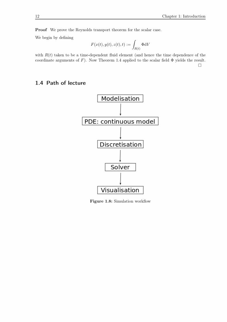
1.4 Path of lecture
Figure 1.8: Simulation workflow

13
2 The equation of fluid flow - Introduction
to modelling
In this chapter, we will especially adress aspects of modelling phenomena in fluid mechanics.In this context, it is essential to deal with the question, how to model mechanical properties ofa fluid, so, as a consequence, also aspects of elasticity/plasticity will occur.
It shall be emphasised that this chapter is only an introduction to modelling; due to thecomplexity of the subject, many interesting and important aspects still are object of researchand a detailed presentation is beyond the scope of the lecture.
We describe the state of a fluid by its state variables. To characterise the fluid flow, in generalthe following state variables need to be considered:
• velocity of the fluid v(x, t),
• density of the fluid ρ(x, t),
• temperature of the fluid T (x, t) and
• pressure p(x, t).
In the case of a three-dimensional flow, we need to model six equations to describe the six statevariables. Depending on the physics of the considered problem, it can be well-motivated toassume some of the variables, for example density or temperature, to be constant or negligible.
The modelling is done by considering conservation principles.
2.1 Lagrangian and Eulerian Systems: Substantial Derivative
In the study of fluid motion there are two main approaches to describing the fluid behaviour:Lagrangian versus Eulerian viewpoint.
2.1.1 The Lagrangian viewpoint
The Lagrangian viewpoint consists of following the material particles of the continuum in theirmotion.
ϕ : Rd × [T0, Tfinal] → Rd × [T0, Tfinal]
(X, t) 7→ ϕ(X, t) = (x, t)
The mapping ϕ allows to link X and x during time by the law of motion, namely
x = x(X, t), t = t,

14 Chapter 2: The equation of fluid flow - Introduction to modelling
Figure 2.1: Lagrangian viewpoint
Figure 2.2: Lagrangian versus Eulerian viewpoint
which explicitly states the particular nature of ϕ: first, the spatial coordinate x depends onboth the material particle X and time t, and, second, physical time is measured by the samevariable t in both material and spatial domains.
Obviously, the one-to-one mapping ϕ must verify
det
(∂x
∂X
)
> 0
in order to impose a one-to-one correspondence (non zero) and to avoid change of orientationin the reference axes (positive). In order to obtain a complete description of the flow field, itis necessary to track a very large number of fluid particles. In engineering applications there istypically a need to know the fluid properties at a given point or location independently fromthe origin of the particles.
2.1.2 The Eulerian viewpoint
The Eulerian description corresponds to a coordinate system fixed in space, and in which fluidproperties are studied as functions of time as the flow passes fixed spatial locations.
2.1.3 The substantial derivative
Definition 2.1 (Substantial derivative) The substantial derivative of any fluid property
f(x, y, z, t)
in a flow field with velocity U = (u, v, w)⊤ is given by
dtf = ∂tf + u∂xf + v∂yf + w∂zf = ∂tf +U · ∇f.
We recall, that the operator ∇ is a vector differential operator ∇ = (∂x, ∂y, ∂z)⊤.
2.2. Conservation of mass 15
(x, y, z) at time t in the Lagrangian viewpoint is defined as
x = x(X, t),
y = y(X, t),
z = z(X, t).
Therefore,f (x (X, t) , y (X, t) , z (X, t) , t)
and it follows
dtf = ∂xf∂tx+ ∂yf∂ty + ∂zf∂tz + ∂tf
= ∂xfu+ ∂yfv + ∂zfw + ∂tf
= ∂tf +U · ∇f.
The last term on the right hand side is related to the transport of the property f with thevelocity field U.
2.2 Conservation of mass
The equation describing the conservation of mass is called continuity equation. If mass isconserved, then the value of change of mass within a control volume V ⊂ R
d needs to be equalto the mass flux over the boundary ∂V (cf. Theorem 1.4):
d
dt
∫
V
ρdx = −
∫
∂V
(ρv) · ndo
with the velocity vector v and the outward unit vector n perpendicular to ∂V .
The divergence theorem (Gauss‘s theorem) implies∫
V
∂tρ+ div (ρv)dx = 0.
Because V is an arbitrary control volume, the equation above needs to hold for all controlvolumes V (especially for arbitrary small ones). It follows, that it holds pointwise:
∂tρ+ div (ρv) = 0. (2.1)
This is the first equation of mathematical fluid mechanics, the continuity equation.
For an incompressible (and homogeneous) fluid, i.e.
ρ(x, t) ≡ ρ0 = const.,
the continuity equation reduces todiv v = 0,
which is a constraint to the velocity field v.
Simplified spoken: If a force tries to compress an incompressible fluid, not its density, but thepressure increases. This happens for instance in water: Water is relatively heavy, so its weightby itself exerts a force that cannot be neglected. The density of water at the ground of theocean is practically the same as at the surface, but the pressure in the depth is much higherthan at the surface.

16 Chapter 2: The equation of fluid flow - Introduction to modelling
2.3 Conservation of momentum
Conservation of momentum means that the rate of change of the linear momentum equals thesum of the forces acting on a set of fluid particles or
force = mass × acceleration.
Consider a fluid particle. If its position at time t is x, i.e. (x, t), then at time t+t (up to thelinear approximation) its position is
(x+ v∆t, t+∆t).
Consequently, its acceleration is
dv
dt= lim
∆t→0
v (x+ v (x, t)∆t, t+∆t)− v(x, t)
∆t= ∂tv +
∑
j
vj∂jv = ∂tv + (v · ∇)v.
This derivative is called material derivative. The nonlinear advective term is in cartesianrepresentation
(v · ∇)v = ∇v · v =
∂1v1 ∂2v1 ∂3v1
∂1v2 ∂2v2 ∂3v2
∂1v3 ∂2v3 ∂3v3
·
v1
v2
v3
.
Therefore, the product of mass and acceleration in volume V equals
∫
V
ρ (∂tv + (v · ∇)v) dx,
which we need to balance with external (volume) forces and internal forces, which act on thevolume.
External forces comprise gravity, buoyancy, Coriolis force and electromagnetic forces (in liquidmetals). They are collected in a volume force term, whose net force on the volume V is givenby
∫
V
ρfdx.
Internal forces are forces, which the fluid exerts on itself, while it tries to get out of its ownway, as for instance friction, pressure, stress or strain. Internal forces are contact forces: Theyact on the surface of the fluid element V . If σ denotes this internal force vector, then the netcontribution of the internal forces equals
∫
∂V
σdo.
This yields the momentum equation for all control volumes V :
∫
V
ρ (∂tv+ (v · ∇)v) dx =
∫
V
ρfdx+
∫
∂V
σdo. (2.2)
To get a local, pointwise equation (for instance a partial differential equation) out of sucha balance equation, the general plan is to describe the balance equation by a single volumeintegral over V . As this equation, again, needs to hold for arbitrary - in particular arbitrary
2.3. Conservation of momentum 17
small - control volumes, it follows, that the equation has to hold pointwise. To enable this planbeing successful, the last integral
∫
∂V
σdo
has to be replaced by a volume integral over V . For this purpose, we need more informationconcerning the internal forces σ.
The correct modelling of the internal forces is a crucial step on the way to predict the flow ofa fluid correctly. So, we will have a closer look at this topic in the course of this chapter.
2.3.1 Conservation of angular momentum
The angular momentum with respect to the origin for a material volume V = V (t) is definedas
L(V ) :=
∫
V
x× (ρv)dx
and its torque as
D(V ) :=
∫
V
x× (ρf)dx+
∫
∂V
x× (n · σ)do.
The conservation law of angular momentum states, that
dtL(V ) = D(V ).
To simplify the notation, we introduce the permutation tensor ε := (εijk)3i,j,k=1 with elements
εijk ∈ −1, 0, 1, depending, if ijk is an odd, no or an even permutation of 1, 2, 3. Then itholds
(x× a)i = εijkxjak ∀x,a ∈ R3.
The transport theorem 1.4 with Φ = εijkxjρvk now implies, that
dtL(V ) =d
dt
∫
V
εijkxjρvkdx =
∫
V
∂t (εijkxjρvk) + div (εijkxjρvkv)dx. (2.3)
The following identities hold:
1.
∂t (εijkxjρvk) = εijkxjvk∂tρ+ εijkρxj∂tvk
2.
div (εijkxjρvkv) = ∂l (εijkxjρvkvl) = εijkxjvkdiv (ρv) + εijkρxjvl∂lvk + εijkρvjvk,
where we used, that
∂ixj = δij .
3.
v × v = 0.

18 Chapter 2: The equation of fluid flow - Introduction to modelling
With these three identities, (2.3) can equivalently be written as
dtL(V ) =
∫
V (t)(x× v) ∂tρ+ (ρx)× ∂tv+ (x× v) div (ρv) + (ρx)× (v · ∇)v dx.
Assuming that the continuity equation
∂tρ+ div (ρv) = 0
holds, we obtain
dtL(V ) =
∫
V
x× (ρ∂tv + ρ (v · ∇)v) dx.
Theorem 1.3 implies that the second term in the definition of D(V ) can be transformed to
∫
∂V
εijkxjnlσlkdo =
∫
V
εijk∂l (xjσlk) dx
=
∫
V
εijkσjk + εijkxj∂lσlk dx
=
∫
V
(ε : σ)i + (x× div σ)idx.
Definition 2.2 (Frobenius (inner/scalar) product) Let A := (aij) ∈ Rm×n and B :=
(bij) ∈ Rm×n be real matrices. The Frobenius (inner/scalar) product of A and B is defined as
A : B :=
m∑
i=1
n∑
j=1
aijbij .
Combining everything, we obtain
∫
V
x× (ρ∂tv + ρ (v · ∇)v) dx =
∫
V
x× (ρf + div σ) + ε : σ dx.
Assuming that conservation of momentum
ρ∂tv + ρ (v · ∇)v = ρf + div σ
holds, we obtain
ε : σ = 0.
It follows with the permutation tensor property of ε that
σjk − σkj = 0,
i.e., the conservation of angular momentum implies the symmetry of the stress tensor :
σ = σ⊤. (2.4)
2.3.2 Conservation of energy
The first law of thermodynamics states that
δU = δQ+ δW,

2.3. Conservation of momentum 19
where U denotes the energy, W the work and Q the heat in a medium. Applied to configurationsof fluid mechanics, the first law of thermodynamics leads to the postulate of a density of internalenergy e = e(x, t), such that the internal energy of a material volume V = V (t) can be expressedas
Eint(V ) :=
∫
V
ρedx.
Its kinetic energy at time t is
Ekin(V ) =1
2
∫
V
ρ ‖v‖2 dx.
The temporal change in total energy
dtE (V (t)) = dt (Eint(V ) + Ekin(V ))
has to be equal to the power of the acting mass forces and stresses
P (V ) :=
∫
V
ρf · vdx+
∫
∂V
n · σ · vdo,
and, additionally, the energy addition by heat sources and less the loss of energy due to heatoutflow
Z(V ) :=
∫
V
ρhdx−
∫
∂V
q · ndo,
where h(x, t) denotes the heat sources/sinks within the volume V and q(x, t) the heat fluxacross the boundary ∂V .
Remark 2.3 1. The contribution of power is caused by translation, i.e.,
P = F · v,
where P denotes the power, F the acting forces and v the velocity of the material.
2. In this energy balance we neglect the energy loss due to radiation.
Combining everything, we obtain the conservation equation
dt (Eint(V ) + Ekin(V )) = P (V ) + Z(V ). (2.5)
Application of the transport theorem 1.4 to Φ = 12ρ ‖v‖
2 and Φ = ρe yields
dtEkin(V ) =
∫
V
1
2∂t
(
ρ ‖v‖2)
+1
2div
(
ρ ‖v‖2 v)
dx,
dtEint(V ) =
∫
V
∂t (ρe) + div (ρev)dx.
Inserting these identities and the definitions of P (V ) and Z(V ) into (2.5) results in
∫
V
∂t
(
ρe+1
2ρ ‖v‖2
)
+ div
(
ρev +1
2ρ ‖v‖2 v
)
dx
=
∫
V
ρf · v + ρh dx+
∫
∂V
n · (σ · v− q) do
=:AV +A∂V .
The surface integral A∂V can be transformed via Theorem 1.3 - utilizing the symmetry of σ -into
A∂V =
∫
∂V
nj (σijvi − qj) do =
∫
V
∂j (σijvi − qj) dx =
∫
V
div (σ · v − q) dx.

20 Chapter 2: The equation of fluid flow - Introduction to modelling
All in all, we obtain
∫
V
∂t
(
ρe+1
2ρ ‖v‖2
)
+ div
(
ρev +1
2ρ ‖v‖2 v
)
dx
=
∫
V
ρf · v + ρh+ div (σ · v − q) dx,
and, pointwise, the general conservation equation of total energy (energy equation)
∂t
(
ρe+1
2ρ ‖v‖2
)
+ div
(
ρev +1
2ρ ‖v‖2 v
)
= ρf · v + ρh+ div (σ · v − q) . (2.6)
Therefore, the temporal and spatial change in total energy ρe+ 12ρ ‖v‖
2 is determined by theexternal sources ρh, the increase in heat due to mechanical power ρf · v + div (σ · v) and thediffusive heat flux div q.
Assuming, that both the continuity equation (2.1) and the conservation equation of momentum(2.2) hold, (2.6) can be reduced to
∂t (ρe) + div (ρev) = σ : ∇v− div q + ρh.
2.3.3 Balance equations
We summarize the equations that we derived so far. For the conservation quantities
• ρ density of mass,
• ρv = (ρvi)3i=1 momentum,
• ρE density of (total) energy,
we derived the following equations based on fundamental conservation principles:
1. Continuity equation for density ρ (conservation of mass):
∂tρ+ div (ρv) = 0.
2. Momentum equation for momentum ρv (conservation of momentum):
∂t (ρv) + div (ρv ⊗ v)− div σ = ρf.
3. Energy equation for density of total energy E := e+ 12 ‖v‖
2 (conservation of energy):
∂t (ρE) + div (ρEv) = ρf · v + div (σ · v) + ρh− div q.
The above variables are also called conservative variables and the corresponding equationsconservation equations.
2.3.4 Kinematic properties
Exterior loads cause displacements of mass points and as a consequence geometric deformationsand strains, respectively, of a mass volume. These changes in structure cause internal counterforces which act against the external loads and balance those in a new resting state. In orderto describe these relations mathematically, we first define the notion of strain.

2.3. Conservation of momentum 21
Figure 2.3: Derivation of the strain tensor of structural mechanics
2.3.4.1 Strain tensor of structural mechanics
The deformation ξ 7→ x = ξ + u(ξ), where ξ denotes the position of a material point inrest position and u the deformation of the material, causes the material volume to change itsgeometry. This process is called strain. It is our goal to describe strain in a fixed point ξ.
Consider an arbitrary directional vector e ∈ R3, ‖e‖ = 1, and a material line element with
endpoints ξ and ξs := ξ + se. Caused by the deformation, the endpoints ξ, ξs pass on to
x = ξ + u(ξ), xs := ξs + u(ξs).
Then the limit
de(ξ) := lims→0
‖x− xs‖ − ‖ξ − ξs‖
‖x− xs‖
describes the relative elongation of the material volume in the image point x(ξ, t) in directione. With the Jacobian matrix ∇u(ξ) it holds
de(ξ) = lims→0
1
s‖se+ u(ξs)− u(ξ)‖
− 1
= ‖e+∇u(ξ)e‖ − 1
= (e+∇u(ξ)e, e+∇u(ξ)e)1
2 − 1
=(
1 +(
∇u(ξ) +∇u(ξ)⊤ +∇u(ξ)⊤∇u(ξ)
e, e)) 1
2
− 1.
The matrix
ǫ(ξ) :=1
2
∇u(ξ) +∇u(ξ)⊤ +∇u(ξ)⊤∇u(ξ)
with the elements
ǫij(ξ) =1
2
∂jui + ∂iuj(ξ) +∑
k
(∂iuk(ξ)∂juk(ξ))
is called strain tensor (with respect to the ξ coordinate system of the rest position). The straintensor associates every direction e in point ξ with a vector ǫ(ξ)e, which describes the strainaccording to
de(ξ) = (1 + 2 (ǫ(ξ)e, e))1
2 − 1.
Especially, for e = ei one obtains the so called principal strains
d(i)(ξ) = (1 + 2ǫii(ξ))1
2 − 1, ǫii(ξ) :=(ǫ(ξ)ei, ei
)(i = 1, 2, 3).

22 Chapter 2: The equation of fluid flow - Introduction to modelling
Figure 2.4: Interpretation of off-diagonal elements
To give an interpretation of the off-diagonal elements ǫij(ξ) (i 6= j), we consider two pointsP := ξ + sei and Q := ξ + sej in the plane spanned by e
i and ej , which form with ξ a right
angle. Then the angle ωij(s) formed by the image segments x(P ) − x(ξ) and x(Q) − x(ξ) isdefined by
cos (ωij(s)) :=(x(P )− x(ξ), x(Q)− x(ξ))
‖x(P )− x(ξ)‖ ‖x(Q)− x(ξ)‖.
Furthermore, it holds (exercise!)
lims→0
1
sx(P )− x(ξ) = (I +∇u(ξ)) ei, lim
s→0
1
s‖x(P )− x(ξ)‖ = 1 + d(i),
lims→0
1
sx(Q)− x(ξ) = (I +∇u(ξ)) ej, lim
s→0
1
s‖x(Q)− x(ξ)‖ = 1 + d(j).
Consequently, one obtains for the so called shear strain (local change in angle) in the pointx(ξ) in the
(ei, ej
)plane:
cos(ωij) = lims→0
cos (ωij(s)) =2ǫij
(1 + d(i)
) (1 + d(j)
) .
The meaning of the strain tensor’s elements becomes clearer, if we restrict ourselves to verysmall strains, i.e., ‖∇u‖ ≪ 1. In this case, we obtain by an approximation of first order:
d(i) ≈ ǫii (≈ 0)
and (by a Taylor expansion of the cosine function)
ωij −π
2≈ cos(ωij) ≈ 2ǫij (i 6= j).
Next, we consider the change in volume caused by the strain. Let Vξ be a volume fixed at thepoint ξ0. Using
det(x′(ξ)
)= det (I +∇u(ξ)) ,
we obtain:
lim|Vξ|→0
|Vx| − |Vξ|
|Vξ|= lim
|Vξ|→0
∫
Vxdx−
∫
Vξdξ
∫
Vξdξ
= lim|Vξ|→0
∫
Vξdet (x′(ξ)) dξ −
∫
Vξdξ
∫
Vξdξ
= det (I +∇u(ξ0))− 1.

2.3. Conservation of momentum 23
In the case of very small strains, i.e., ‖∇u‖ ≪ 1, Taylor expansion yields
det (I +∇u(ξ))− 1 = det(I)︸ ︷︷ ︸
=1
+det′(I)∇u(ξ) +O(
‖∇u(ξ)‖2)
− 1.
The partial derivatives of the determinant of a matrix with respect to its elements are given bythe cofactors of the matrix:
∂
∂aijdet(A) = (−1)i+jco(aij), i, j = 1, 2, 3,
where co(aij) is obtained as the determinant of the matrix that results if one sweeps the ithrow and the jth column of A. Therefore, it holds
det (I +∇u(ξ))− 1 =∑
i,j
((−1)i+jco(δij)∂jui(ξ)
)+O
(
‖∇u(ξ)‖2)
=∑
i,j
(δij∂jui(ξ)) +O(
‖∇u(ξ)‖2)
=∑
i
(∂iui(ξ)) +O(
‖∇u(ξ)‖2)
= div u(ξ) +O(
‖∇u(ξ)‖2)
.
Since the trace of a tensor is invariant to rotations of the coordinate system, also the relativechange in volume is invariant to rotations of the coordinate system (as expected).
2.3.4.2 Strain tensor of fluid mechanics
It is a typical property of fluid flow that even small acting forces result in arbitrary largedisplacements of the material points which is nothing else but the flow. In contrast to structuralmechanics, not the deformation itself is of importance but the velocity at which the deformationhappens.
For the specification of the term strain velocity we consider again an arbitrary directional vectore ∈ R
3, ‖e‖ = 1, and a material line element with endpoints x and xs := x+ se at time t, cf.Figure 2.5. After a time interval k = ∆t the endpoints passed on to the locations
y = x+ v(x, t)k + δ(x, k), ys = xs + v(xs, t)k + δ(xs, t),
where the remainders are of order O(k2). The relative elongation in direction e at time t+ k
is then given by
de(x, t+ k) = lims→0
‖y − ys‖ − ‖x− xs‖
‖x− xs‖,
and the relative velocity of elongation at time t becomes
de(x, t) = limk→0
de(x, t+ k)
k.
Obviously, it holds
‖y − ys‖ − ‖x− xs‖
‖x− xs‖=
‖se− v(x, t) − v(xs, t) k + δ(xs, k)− δ(x, k)‖
s− 1.

24 Chapter 2: The equation of fluid flow - Introduction to modelling
Using the fact, that
lims→0
‖δ(xs, k)− δ(x, k)‖
s= O
(k2),
we obtain
de(x, t+ k) =∥∥e+
∇vk +O
(k2)
e∥∥ − 1
=
1 +(
k
∇v+∇v⊤
e+O(k2)e, e) 1
2
− 1.
Applying the approximation
(1 + z)1
2 = 1 +z
2+O
(z2)
yields
de(x, t) =1
2
(
∇v +∇v⊤
e, e)
.
The tensor
ǫ(x, t) :=1
2
∇v(x, t) +∇v⊤(x, t)
(2.7)
is called rate of deformation tensor (with respect to the x coordinate system which is fixed inspace).
Therefore, the velocity of elongation with respect to direction e can be expressed as
de(x, t) = (ǫ(x, t)e, e) .
Especially, we obtain the relative velocity of elongation in direction of ei as
ǫii = ∂ivi, i = 1, 2, 3,
the relative rate of change in angle in the (ei, ej) plane as
ǫij =1
2∂jvi + ∂ivj ,
and, finally, the relative rate of change in volume
trace(ǫ) = div v.
2.3.4.3 Optional: Derivation of rotational and strain velocities according to [7]
The gradient tensor of velocity ∇v contains information about the (local) spatial changes ofthe velocity field. Consequently, it plays an important role, if we ask how infinitesimal adjacentmaterial points are displaced in a relative view.
We denote the components of the velocity field v by
v = (u, v, w)⊤ .
We consider two points „1“ and „2“, positioned at r and r+ dr, respectively. During the timeinterval ∆t, in linear approximation, they are shifted by v1∆t and v2∆t, respectively. Theirrelative position at the time t+∆t is thus given by the vector
dr∗ = dr+ (v2 − v1)∆t+O(∆t2
)(2.8)
(see figure 2.5).

2.3. Conservation of momentum 25
Figure 2.5: Displacement of infinitesimal adjacent points.
Now we have for the difference of the velocity components of the two infinitesimal adjacentpoints
u2 − u1 = ∂xudx+ ∂yudy + ∂zudz
v2 − v1 = ∂xvdx+ ∂yvdy + ∂zvdz
w2 −w1 = ∂xwdx+ ∂ywdy + ∂zwdz
or
v2 − v1 = ∇v · dr.
Using (2.8) we achieve
dr∗ − dr = ∇v · dr∆t+O(∆t2
).
The left-hand side describes the change of the distance vector to point „2“ in the time interval∆t, an observer moving with the material point „1“ sees. Dividing by ∆t and then evaluatingthe limit for ∆t→ 0 gives the following fundamental relation for infinitesimal adjacent materialline elements:
dt (dr) = ∇v · dr. (2.9)
So, the tensor ∇v transforms the relative position vector dr into its material derivative.
We now split ∇v into a symmetric part D (with D⊤ = D) and a skew symmetric part W (withW⊤ = −W ) via
D :=1
2
(
∇v + (∇v)⊤)
, W :=1
2
(
∇v− (∇v)⊤)
. (2.10)
Remark 2.4 By representing D and W in cartesian coordinates, the following properties showup:
• The sum of the diagonal elements, i.e. the trace, of D corresponds to the divergence ofthe velocity field
div v.

26 Chapter 2: The equation of fluid flow - Introduction to modelling
Figure 2.6: Temporal change of two material line elements.
• In W the components of the so called vorticity vector
ω := rot v
can be found and for an arbitrary vector b it holds
W · b =1
2ω × b.
By splitting ∇v = D +W , the right-hand side of (2.9) decomposes into two summands, thatinfluence the time derivative additively.
For the contribution from W it holds with remark 2.4
dt (dr) =1
2ω × dr,
which is nothing different than a rotation of dr with the angular velocity ω2 . As a consequence,
the tensor W is called spin tensor.
To interpret the tensor D we consider the change in time of the inner product of two materialline elements dr and δr with length ds and δs, respectively, that enclose the angle 90 − γ.By
dt(dr · δr) = dt(dsδs sin γ)
applying the chain rule for derivatives, using (2.9), (2.10) and doing some basic transformations,one arrives at
dt(ds)
ds+
dt(δs)
δs
sin γ + dtγ cos γ = 2dr
ds·D ·
δr
δs. (2.11)
To filter a diagonal element, say Dxx, out of the right-hand side, we let the line elementscoincide and choose their orientation (for this example) along the x-axis. On these conditions,the enclosed angle vanishes, i.e. γ = 90, and (2.11) reduces to
dt(ds)
ds= Dxx.
This relation shows that the diagonal elements of the tensor D give the elongation rate of suchline elements that currently are oriented in the direction of the basis vectors.

2.3. Conservation of momentum 27
Analogously, it is possible to filter out an offdiagonal element out of the right-hand side of(2.11), by choosing line elements perpendicular to each other and oriented parallel to basisvectors ei. Then, γ = 0 and (2.11) reduces for instance to
dtγ = 2Dxy.
The offdiagonal elements therefore have half the magnitude of the velocities that describe thechange of the angle between two line elements, which at the present are oriented parallel todifferent basis vectors. Thus, the tensor D describes the elongation rates of the edges and therate of change of the angles between the edges of a momentarily box-shaped material volumeelement with an orientation parallel to the coordinate axes. Consequently, D is called rate ofdeformation tensor.
2.3.5 Material properties
2.3.5.1 Surface forces
Hydrostatic pressure:σ|v=0 = −pI.
Case of non-static fluid:σ = −pI + τ,
where τ denotes the shear tensor . The tensor τ depends on the deformation of the fluid: withthe deformation tensor ǫ = 1
2
(∇v+∇v
⊤), the trial for τ reads
τ = F (ǫ).
Assumptions: (material assumptions)
1. F (0) = 0.
2. Symmetry: we assume thatτ = τ⊤.
3. Isotropy: invariance with respect to orthogonal transformations, i.e.,
F(
QǫQ⊤)
= QF (ǫ)Q⊤,
where Q is an orthogonal matrix, i.e.,
QQ⊤ = I, det(Q) = 1.
Theorem 2.5 (Material tensor) Assuming the above assumptions on the material, then
F (ǫ) = ϕ0I + ϕ1ǫ+ ϕ2ǫ2,
where ϕi(I1, I2, I3) and
I1 = trace(ǫ),
I2 =1
2ǫij ǫji − ǫiiǫjj ,
I3 = det(ǫ).

28 Chapter 2: The equation of fluid flow - Introduction to modelling
Proof We assume ǫ to be a 3× 3 tensor/matrix with eigenpairs
(λi, ei)1≤i≤3 , λi ∈ R, ei ∈ R3.
1. We prove that e1, e2, e3 are eigenvectors of F (ǫ).
We consider Q the orthogonal transformation of 180 rotation around e3.
Qǫ = ǫQ,
QǫQ⊤ = ǫ.
Due to the isotropy condition
F (ǫ) = F(
QǫQ⊤)
= QF (ǫ)Q⊤,
F (ǫ)Q = QF (ǫ).
Let W = [e1, e2, e3].
F (diag(λi)) = F(
WǫW⊤)
=WF (ǫ)W⊤ = diag(µi).
2. We assume that the eigenvalues λi1≤i≤3 are simple eigenvalues (multiplicity = 1).
det
1 λ1 λ211 λ3 λ231 λ3 λ23
6= 0
ϕ0 + ϕ1λ1 + ϕ2λ21 = µ1(λ1, λ2, λ3)
ϕ0 + ϕ1λ2 + ϕ2λ22 = µ2(λ1, λ2, λ3)
ϕ0 + ϕ1λ3 + ϕ2λ23 = µ3(λ1, λ2, λ3)
This linear system has a unique solution ϕi = ϕi(λ1, λ2, λ3) = ϕi(I1, I2, I3). Due to theorthogonality of the eigensystem e1, e2, e3 we obtain
F (ǫ) = ϕ0I + ϕ1ǫ+ ϕ2ǫ2.
Remark 2.6 The assumption on the simplicity of the eigenvalues in step 2 can be obtained –if needed – by means of an infinitely small perturbation of ǫ.
So far, we have derived from the material assumptions, that
σ = −pI + F (ǫ)
= −pI + ϕ0I + ϕ1ǫ+ ϕ2ǫ2.
If the fluid is assumed to be Newtonian, the term ϕ2ǫ2 is neglected. Consequently, the stress
tensor σ becomes a linear relation.
Now, we switch from mathematics to physics and write the relation for a Newtonian fluid as
σ = −pI + 2µǫ+ λtr(ǫ)I

2.3. Conservation of momentum 29
with the shear viscosity µ and the volume viscosity λ. The shear viscosity describes how viscousa fluid is and can be measured. The volume viscosity indicates the relation between changeof temperature and change of volume; as in this lecture, temperature will be considered asconstant, we will not care about λ.
Now, assuming ρ(x, t) = ρ0:
∂u
∂t−
(µ
ρ0
)
∆u+ (u · ∇)u+∇
(p
ρ0
)
= f
∇ · u = 0
we achieved the unsteady incompressible Navier-Stokes equations that provide 3+1 equationsfor 3+1 variables (u, p).
Remark 2.7 What is the optimal wind direction to move your sailing boat at highest speed?perpendicular to the direction of motion; cf. airplane wings: Different velocities before and be-hind the sail lead to different pressures leading to forces that move the boat fast. Unfortunately,this solution is unstable.
2.3.5.2 Reynolds number
We assume that the flow occurs in a domain Ω and the flow geometry has some characteristiclength L. For example, L can be the length of an airplane.Thus, we can geometrically scale the domain to get a rescaled domain Ω∗ = Ω
L. Ω and Ω∗ are
geometrically similar.
x∗ =x
L, L : reference length
u∗ =u
V, V : reference speed
t∗ = V ·t
L,
p∗ =p
ρ0V 2
V is a reference speed, for example the free stream speed away from the model airplane.If we denote partial derivatives with respect to the rescaled dimensionless variables by ∂
∂x∗ ,then the chain rule implies
∂u∗
∂x∗=L
V
∂u
∂xfor example.
The Navier-Stokes equations for incompressible flows in the rescaled variables becomes
∂u∗
∂t∗−
(µ
ρ0V L
)
∆∗u∗︸ ︷︷ ︸
viscous forces
+(u∗ · ∇∗)u∗︸ ︷︷ ︸
inertial forces
+∇∗p∗ = f
∇∗u∗ = 0.
Definition 2.8 (Dynamic similarity) Flows in similar geometry Ω and Ω∗ = ΩL
are dynam-ically similar, if the parameters of the flow are such that the quantities of the flows
Re =ρ0V L
µ(2.12)
coincide.The dimensionless parameter Re is called the Reynolds number.

30 Chapter 2: The equation of fluid flow - Introduction to modelling
Figure 2.7: Poiseuille flow.
Remark 2.9 A step function (eg. deriving from an earth quake) will remain unchanged duringtime passing by, as long as the viscous forces are neglected. But taking the viscous forces intoconsideration leads to a smoothing of the function after some time.
Remark 2.10 The dynamic similarity can be very usefull: To verify for instance your simula-tion results of an airplane, instead of building the airplane in full size, you can build a smallermodel and adapt the other parameters (increase V or decrease µ) in such a way that Re is keptconstant.
Re =inertial forces
viscous forces
If Re is close to 0, the viscous forces dominate inertial forces, as occurs in a highly viscous fluidmoving slowly.For very large Reynolds numbers the viscous forces can be neglected. This often occurs in flowsof gases.
Examples:
• model airplane, 1 ms−1: Re ∼ 104
• car, 3 ms−1: Re ∼ 105
• small airplane, 30ms−1: Re ∼ 107
2.3.5.3 Poiseuille flow
At low velocities, one has a laminar flow. By increasing the velocity, eventually one reaches thecritical Reynolds number where turbulences occur and the flow gets chaotic.
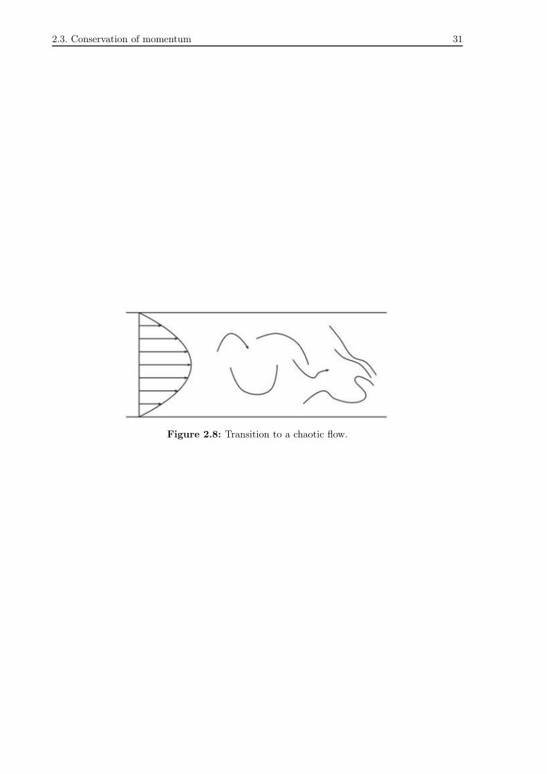
2.3. Conservation of momentum 31
Figure 2.8: Transition to a chaotic flow.

33
3 Approximating Steady Flows
This chapter considers the problem of approximating a steady solution (v, p) of the Navier-Stokes equations (NSEs):
−ν∆v+ (v · ∇)v +∇p = f, in Ω
div v = 0, in Ω
v = 0, on ∂Ω∫
Ω pdx = 0.
(3.1)
The steady NSE present the two interesting problems of stability bounds for the pressure(coupling between div v = 0 and ∇p), which, mathematically, is equivalent to a saddle-pointproblem, and stability bounds for the velocity (due to the nonlinearity). In the methods weconsider, boundedness of the pressure by problem data is ensured by using elements whichsatisfy the so called discrete inf − sup condition. It is a discrete analog to the inf − sup sta-bility condition which is needed in the (weak) continuous theory to ensure boundedness of thecontinuous pressure. The other main difficulty is the nonlinearity. The solution of this prob-lem which ensures the physical energy bounds hold for approximate solutions is to explicitlyskew-symmetrize the nonlinearity in the equations for the approximate solution.
3.1 The Stokes problem: Introduction to Mixed Methods
In this section we study the Stokes problem which is a simplification of NSE. It is the „sim-plest“ subproblem of the full NSE where the conditions for the stability bounds for the pressurecan be established. As we will see later, the solution to this problem in the case of the Stokesproblem is also a solution in the case of the nonlinear NSE.
The Stokes problem consists of finding the fluid velocity v : Ω → Rd and pressure p : Ω → R
defined in the flow domain Ω ⊂ Rd satisfying
−∆v +∇p = f, in Ω
div v = 0, in Ω
v = 0, on ∂Ω
(3.2)
Note that ∇p occurs in the Stokes problem rather than p and that there is (under the above mostcommon boundary conditions at least) no pressure boundary condition. Thus, the pressure can,at best, be determined only up to an additive constant
∇(p+ C) = ∇p.
For this reason the pressure is normalized in some way to determine the arbitrary additiveconstant; the most mathematically convenient way is by
∫
Ωpdx = 0.

34 Chapter 3: Approximating Steady Flows
First, we derive a variational formulation of (3.2). Let (v, p) be a classical solution of the Stokesproblem. Multiply (3.2) by (smooth enough) functions (ϕ, q) and integrate:
∫
Ω (−∆v · ϕ+∇p · ϕ) dx =∫
Ω f · ϕdx,∫
Ω div vqdx = 0.
Applying the divergence theorem 1.3, term by term, gives
−
∫
Ω∆v · ϕdx =
∫
Ω∇v : ∇ϕdx−
∫
∂Ω∇v · ϕ · ndo.
If ϕ vanishes on ∂Ω we thus have
−
∫
Ω∆v · ϕdx =
∫
Ω∇v : ∇ϕdx.
Similarly, if ϕ again vanishes on ∂Ω,
∫
Ω∇p · ϕdx = −
∫
Ωpdiv ϕdx.
Thus, for all ϕ vanishing on ∂Ω and smooth enough and all q smooth enough, (v, p) satisfies
∫
Ω (∇v : ∇ϕ− pdiv ϕ) dx =∫
Ω f · ϕdx∫
Ω div vqdx = 0.(3.3)
The last system of equations is still well-defined in the following function spaces: Define thevelocity space X as
X :=(H1
0 (Ω))d
=(v ∈ C1(Ω) : v ∈ L2(Ω), ∂iv ∈ L2(Ω) ex. in weak sense ∀i, v = 0 on ∂Ω
)d.
The pressure space Q does not require any differentiability since no derivatives of p or q appearin (3.3). On the other hand, it must account for the fact that if (v, p) is a solution of (3.2),then so is (v, p + C) for any constant C. Accordingly, to fix the value of the undetermined,additive constant it is usual to impose the condition of mean value zero and thus define
Q := L20(Ω) =
q ∈ L2(Ω) :
∫
Ωqdx = 0
.
We thus come to the variational formulation of (3.2):
Find v ∈ X, p ∈ Q satisfying
(∇v,∇ϕ)− (p,div ϕ) = (f, ϕ) ∀ϕ ∈ X
(div v, q) = 0 ∀q ∈ Q. (3.4)
Lemma 3.1 (Continuity)
b(v, q) :=
∫
Ωdiv vqdx
is continuous on X ×Q:|b(v, q)| ≤ C ‖q‖Q ‖v‖X .
As a consequence the divergence free subspace V of X
V := v ∈ X : (div v, q) = 0 ∀q ∈ Q
is a closed subspace of X.

3.1. The Stokes problem: Introduction to Mixed Methods 35
Proof The inequality is obvious due to Hölder inequality and definitions of the norms. Sinceb(v, q) is bilinear it follows equally easily that V is a subspace. The key to showing V is closedis to use continuity. By continuity, let vn ∈ V be a sequence such that vn → v in X and letq ∈ Q be fixed: then b(vn, q) → b(v, q) for n→ ∞. Since b(vn, q) ≡ 0 it follows from continuitythat b(v, q) = 0, i.e., v ∈ V .
Definition 3.2 For f ∈ L2(Ω), the H−1 norm and the V ∗ norm of f are
‖f‖−1 := supv∈X
|(f, v)|
‖∇v‖, ‖f‖∗ := sup
v∈V
|(f, v)|
‖∇v‖.
Definition 3.3 The function spaces H−1(Ω) and V ∗ are, respectively, the closures of L2(Ω)in, respectively, ‖·‖−1 and ‖·‖∗.
We don’t want to go to far afield into the question of existence of solutions to the Stokesproblem in various function Sobolev spaces with data in other Sobolev spaces. Hoewever, thereis one very important theoretical result (proved by Ladyzhenskaya), the continuous inf − supcondition, which we give here for future reference.
Proposition 3.4 (The continuous inf − sup condition) There is a constant β > 0 suchthat
infq∈Q
supv∈X
(div v, q)
‖∇v‖ ‖q‖≥ β > 0. (3.5)
To indicate the critical importance of the last lemma and proposition, note that the lemmaimplies V is in fact also a Hilbert space. Since div v = 0 (weakly) the solution of the Stokesproblem lies in V . It has thus the following formulation in V :
Find v ∈ V satisfying (∇v,∇ϕ) = (f, ϕ) ∀ϕ ∈ V. (3.6)
In this formulation, existence and uniqueness of v follow from the Lax-Milgram theorem, asdoes the simple bound on the fluid velocity:
‖∇v‖ ≤ ‖f‖∗ .
This bound shows that the velocity is bounded by the body force, the most fundamental ofmany different types of stability. Thus, Lemma 3.1 and the Lax-Milgram theorem immediatelyimply existence of a velocity satisfying the variational formulation of the Stokes problem in V .(The inf − sup condition plays the key role of ensuring that, given the unique velocity, there isa corresponding pressure.)
Proposition 3.5 (Existence) For any f ∈ L2(Ω), there exists a unique velocity in V solvingthe Stokes problem. This velocity satisfies the a-priori bound
‖∇v‖ ≤ ‖f‖∗ .
The inf − sup condition is also critical to bounding the fluid pressure, i.e., showing the pressureis stable in a fundamental sense. To see this, note that the inf − sup condition (3.5) is equivalentto
sup06=v∈X
(div v, q)
‖∇v‖≥ β ‖q‖ for any q ∈ Q.

36 Chapter 3: Approximating Steady Flows
To use this, our strategy is to isolate the (div ϕ, p) term and seek an upper bound resembling
(div ϕ, p) = everything else ≤ · · · ≤ terms ‖∇ϕ‖ .
Next, we divide both sides by ‖∇ϕ‖ and take a supremum over v ∈ X. To be specific,rearranging (3.4)
(p,div ϕ) = (∇v,∇ϕ)− (f, ϕ)
≤ ‖∇v‖ ‖∇ϕ‖ + ‖f‖∗ ‖∇ϕ‖
≤ (‖∇v‖ + ‖f‖∗) ‖∇ϕ‖ .
Thus,
β ‖p‖ ≤ sup06=ϕ∈X
(div ϕ, p)
‖∇ϕ‖≤ (‖∇v‖ + ‖f‖∗) .
The upper bound ‖∇v‖ ≤ ‖f‖∗ gives
‖p‖ ≤2 ‖f‖∗β
.
Thus, adding the bounds for the velocity and pressure together gives
‖∇v‖ + ‖p‖ ≤
(
1 +2
β
)
‖f‖∗ ,
proving a stability bound on the fluid velocity and pressure.
Definition 3.6 (The discrete inf − sup condition) The finite-dimensional spaces Xh ⊂ Xand Qh ⊂ Q fulfil the discrete inf − sup condition, if there is a constant βh > 0 such that
infqh∈Qh
supvh∈Xh
(div vh, qh)
‖∇vh‖ ‖qh‖≥ βh > 0, (3.7)
where βh is bounded away from zero uniformly in h.
Remark 3.7 (Interpretation of discrete inf − sup condition) If (3.4) is discretized withfinite elements, then the system matrix of the discrete system has the following block represen-tation: (
A −BB⊤ 0
)
,
where
A := (aij)i,j , aij := (∇ϕj ,∇ϕi) ,
B := (bij)i,j , bij := (qj,div ϕi) .
For the existence and uniqueness of a discrete solution it is both a necessary and sufficientcondition that the above matrix is regular, i.e., that the discrete linear system has a uniquesolution. The critical part is the „0“ block: if this part of the matrix is too big, then thelinear system is under-determined, i.e., the rows are linearly dependent, and the solution is notunique anymore. If, on the other hand, this block is too small, then there are posed too manyconditions on the velocity and the system contains contradicting rows, i.e., the linear systemis over-determined, and there doesn’t exist any solution. At this point, the discrete inf − supcondition guarantees exactly that the „0“ block has precisely the right size to obtain a regularlinear system!

3.2. Formulation and Stability of the Approximation 37
3.2 Formulation and Stability of the Approximation
We now turn our attention to the NSE again. Analogously to the previous section about theStokes problem, we can derive a weak formulation of the NSE. It reads:
Find v ∈ X, p ∈ Q satisfying
ν (∇v,∇ϕ) + ((v · ∇)v, ϕ)− (p,div ϕ) = (f, ϕ) ∀ϕ ∈ X
(div v, q) = 0 ∀q ∈ Q,
(3.8)with the spaces X and Q defined as above.
The solution of the stated first problem — stability of the pressure — is to use, as for theStokes problem, finite element spaces
Xh ⊂ X, Qh ⊂ Q
satisfying (3.7).
The second problem is treated by carefully formulating the nonlinearity in the discrete problem.To this end, we first state some properties of the trilinear form that is associated with thenonlinearity.
Lemma 3.8 (Skew-symmetry) If v,∇v ∈ L2(Ω), div v = 0 and v · n = 0 on ∂Ω, then itholds ∫
Ωv · ∇v · vdx = 0. (3.9)
More generally, ∫
Ωu · ∇v ·wdx = −
∫
Ωu · ∇w · vdx
for any such u,v,w.
Proof Cf. [9], Chapter 6, Lemma 12.
Remark 3.9 Especially, (3.9) holds for all v ∈ V because v·n vanishes exactly on the boundaryand div v is exactly zero.
Lemma 3.10 (Continuity of the trilinear form) There is a finite constant M = M(Ω)such that for all u,v,w ∈ X,
|((u · ∇)v,w)| ≤M ‖∇u‖ ‖∇v‖ ‖∇w‖ . (3.10)
Proof Cf. [9], Chapter 6, Lemma 13.
Remark 3.11 Since V is a closed subspace of X, the trilinear form is also continuous onV × V × V .
Difficulties can arise because an approximate solution
vh ∈ Vh := v ∈ Xh : (qh,div v) = 0 ∀qh ∈ Qh
is approximately but (except in very special cases) never exactly divergence free:
div vh 6= 0 and Vh * V in general!

38 Chapter 3: Approximating Steady Flows
To formulate the discrete problem so as to eliminate any such potential difficulties, define the(explicitly skew symmetrized) trilinear form
b∗(u,v,w) :=1
2((u · ∇)v,w)−
1
2((u · ∇)w,v) .
We have associated with the nonlinearity the finite continuity constants (which depend on thedomain Ω):
M =M(Ω) := supu,v,w∈X
|((u · ∇)v,w)|
‖∇u‖ ‖∇v‖ ‖∇w‖<∞,
N = N(Ω) := supu,v,w∈V
|((u · ∇)v,w)|
‖∇u‖ ‖∇v‖ ‖∇w‖<∞.
Since V ⊂ X it follows that N ≤M .
Lemma 3.12 (Skew-symmetry and continuity) For u ∈ V , v,w ∈ X,
((u · ∇)v,w) = b∗(u,v,w).
Further,
b∗(u,v,v) = 0 for any u,v ∈ X,
and
|b∗(u,v,w)| ≤M ‖∇u‖ ‖∇v‖ ‖∇w‖ ∀u,v,w ∈ X,
for the same M =M(Ω).
Proof Exercise.
Thus, another variational formulation of a solution of (3.8) which is equivalent for the contin-uous problem is as follows:
Find v ∈ X, p ∈ Q satisfying
ν (∇v,∇ϕ) + b∗(v,v, ϕ) − (p,div ϕ) = (f, ϕ) ∀ϕ ∈ X
(div v, q) = 0 ∀q ∈ Q.
(3.11)The corresponding finite element approximation that we consider reads: Find vh ∈ Xh, ph ∈ Qh
satisfying
ν (∇vh,∇ϕh) + b∗(vh,vh, ϕh)− (ph,div ϕh) = (f, ϕh) ∀ϕh ∈ Xh
(div vh, qh) = 0 ∀qh ∈ Qh
. (3.12)
The formulation (3.12) can be written as follows: Find vh ∈ Vh satisfying
ν (∇vh,∇ϕh) + b∗(vh,vh, ϕh) = (f, ϕh) ∀ϕh ∈ Vh. (3.13)
Lemma 3.13 (Stability) The finite element approximation (3.12) is stable,
ν ‖∇vh‖ ≤ ‖f‖−1 ,
and if (3.7) holds, then
‖ph‖ ≤1
β
(
2 +M
ν2‖f‖−1
)
‖f‖−1 .

3.2. Formulation and Stability of the Approximation 39
Proof For the first result, set ϕh = vh in (3.13). This is equivalent to setting ϕh = vh andqh = ph in (3.12) and adding. Using b∗ (vh,vh,vh) = 0 we get
ν ‖∇vh‖2 = (f,vh) ≤ ‖f‖−1 ‖∇vh‖ ,
giving the first inequality. For the stability bound of the pressure, solve (3.12) for (ph,div ϕh):
(ph,div ϕh) = − (f, ϕh) + ν (∇vh,∇ϕh) + b∗(vh,vh, ϕh),
so(ph,div ϕh) ≤ ‖f‖∗ ‖∇ϕh‖ + ν ‖∇vh‖ ‖∇ϕh‖ +M ‖∇vh‖ ‖∇vh‖ ‖∇ϕh‖ .
Thus,(ph,div ϕh)
‖∇ϕh‖≤ ‖f‖∗ + ν ‖∇vh‖ +M ‖∇vh‖
2 .
Taking the supremum over ϕh ∈ Xh and using ν ‖∇vh‖ ≤ ‖f‖−1 and the assumed condition(3.7) gives the pressure bound.
It is useful to think of the error analysis as a combination of three ideas:
• The Céa’s lemma shows how to handle the contribution of the viscous terms.
• The inf − sup condition shows how to handle the coupling between div v = 0 and ∇p inthe error analysis.
• The small data conditionM
ν2‖f‖−1 ≤ α < 1
will be used to control the nonlinearity in the error analysis.
The error analysis is complex but the underlying ideas are simple: To give some understandinghow to handle the nonlinear terms we first consider an example with contractive properties.
Suppose T : X → X satisfies
‖T (x)− T (y)‖X ≤ α ‖x− y‖X ∀x, y ∈ X
for some α < 1. Let Xh ⊂ X be a subspace. Let x∗ be the unique fixed point of T :
x∗ − T (x∗) = 0.
Let xh ∈ Xh ⊂ X be the Galerkin approximation of x∗
(xh − T (xh), yh) = 0 ∀yh ∈ Xh.
Let us consider the error in x∗:
((x∗ − xh)− (T (x∗)− T (xh)), yh)X = 0.
Thus,((x∗ − xh), yh)X = ((T (x∗)− T (xh)), yh)X .
Let Ph : X → Xh denote the orthogonal projection into Xh. Set yh = Ph(x∗ − xh). Then,
‖Ph(x∗ − xh)‖
2X ≤ α ‖x∗ − xh‖X ‖Ph(x
∗ − xh)‖X .
Thus,‖Ph(x
∗ − xh)‖X ≤ α ‖x∗ − xh‖X .
Furthermore,
‖x∗ − xh‖2X ≤ ‖x∗ − Phx
∗‖2X + ‖Ph(x∗ − xh)‖
2X
≤ ‖x∗ − Phx∗‖2X + α2 ‖x∗ − xh‖
2X .

40 Chapter 3: Approximating Steady Flows
Theorem 3.14 (Error in Galerkin approximation of fixed points) Let x∗ be the uniquefixed point of a contractive map in X with contraction constant α and let xh denote its Galerkinapproximation. Then, the error satisfies:
‖x∗ − xh‖X ≤(1− α2
)− 1
2 infwh∈Xh
‖x∗ − wh‖X .
Theorem 3.15 Suppose the small data condition
Nh
ν2‖f‖h ≤ α < 1,
where
Nh := supuh,vh,wh∈Vh
b∗(uh,vh,wh)
‖∇uh‖ ‖∇vh‖ ‖∇wh‖,
holds. Then there is at most one solution for (3.13).
Proof First, we derive the error equation. This is the nonlinear equivalent of the Galerkinorthogonality.
∀ϕh ∈ Xh, ∀qh ∈ Qh :
ν (∇(v − vh),∇ϕh) + b∗(v,v, ϕh)− b∗(vh,vh, ϕh)− (p,div ϕh) = 0
div v = 0
(div vh, qh) = 0
It’s an important refinement of this equation to note that since vh ∈ Xh, (div vh, qh) = 0, wecan write:
(p,div ϕh) = (p− qh,div ϕh) ∀qh ∈ Qh, ϕh ∈ Xh.
The error equation then becomes
ν (∇(v − vh),∇ϕh)+ b∗(v,v, ϕh)− b∗(vh,vh, ϕh)− (p− qh,div ϕh) = 0 ∀qh ∈ Qh, ϕh ∈ Xh.
1. Write v− vh = (v− ϕh)− (vh − ϕh) = η− φh (where φh ∈ Xh), where ϕh is an optimalapproximation of v in Xh.
2. Put the φh terms on one side and the η term on the other, set ϕh = φh and get a boundof ‖∇φh‖ in terms of ‖∇η‖.
3. Quadratic nonlinearities are usually treated in the following way:
aa− bb = a(a− b) + (a− b)b.
4. Apply Cauchy-Schwartz inequalities to the right-hand side for η and φh. Use the smalldata condition to hide the φh terms.
5. Apply the triangle inequality ‖∇(v − vh)‖ ≤ ‖∇η‖ + ‖∇φh‖.
6. Take the infimum over ϕh ∈ Xh.
Step 1 gives
v− vh = η − φh.
We obtain
ν (∇φh,∇ϕh) =1
Re(∇η,∇ϕh)+b
∗(v,v, ϕh)−b∗(vh,vh, ϕh)−(p− qh,div ϕh) ∀ϕh ∈ Xh, ∀qh ∈ Qh.

3.2. Formulation and Stability of the Approximation 41
Step 2:
ν ‖∇φh‖2 =
1
Re(∇η,∇φh)+b
∗(v,v, φh)−b∗(vh,vh, φh)− (p− qh,div φh) ∀qh ∈ Qh. (3.14)
Step 3:
b∗(v,v, φh)− b∗(vh,vh, φh) = b∗(v,v − vh, φh) + b∗(v − vh,vh, φh)
= b∗(v, η − φh, φh) + b∗(η − φh,vh, φh)
= b∗(v, η, φh) + b∗(η,vh, φh)− b∗(φh,vh, φh).
It follows
|b∗(v,v, φh)− b∗(vh,vh, φh)| ≤M ‖∇v‖ ‖∇η‖ ‖∇φh‖
+M ‖∇vh‖ ‖∇η‖ ‖∇φh‖
+M ‖∇vh‖ ‖∇φh‖2 .
Inserting this bound in (3.14) gives
(ν −M ‖∇vh‖) ‖∇φh‖2 ≤ ν (∇η,∇φh)− (p− qh,div φh) +M (‖v‖ + ‖vh‖) ‖∇η‖ ‖∇φh‖ .
Step 4: Now we use the idea of step 4 (ab ≤ εa2 + 14εb
2)
(ν −M ‖∇vh‖) ‖∇φh‖2 ≤ ε ‖∇φh‖
2
+ν2
4ε‖∇η‖2
+ ε ‖∇φh‖2
+d
4ε‖pqh‖
2
+ ε ‖∇φh‖2
+M2
4ε(‖v‖ + ‖vh‖)
2 ‖∇η‖2 .
It follows
(ν −M ‖∇vh‖ − 3ε) ‖∇φh‖2 ≤
ν2
4ε‖∇η‖2 +
d
4ε‖pqh‖
2 + ε ‖∇φh‖2 +
M2
4ε(‖v‖ + ‖vh‖)
2 ‖∇η‖2 .
Small data condition and ν ‖∇vh‖ ≤ ‖f‖−1 yield
M ‖∇vh‖ ≤MRe ‖f‖−1
≤ α1
Re
≤1
Re.
Thus, we obtain, assuming ε = 1−α6 ν ‖∇φh‖
ν(1− α)
2‖∇φh‖
2 ≤3ν
2(1 − α)‖∇η‖2
+3d
2(1 − α)ν‖p− qh‖
2
+3
2(1 − α)ν
(2
ν‖f‖∗
)2
‖∇η‖2

42 Chapter 3: Approximating Steady Flows
and further
‖∇φh‖2 ≤
3
(1− α)2‖∇η‖2
+3d
(1− α)2ν2‖p− qh‖
2
+12
(1− α)2ν4‖f‖2−1 ‖∇η‖
2 .
Step 5: So we obtain
‖∇(v − vh)‖ ≤ ‖∇η‖ + ‖∇φh‖ .
The result follows with Theorem 3.16.
Theorem 3.16 (Convergence of the FEM) Suppose the global uniqueness condition
M
ν2‖f‖−1 ≤ α < 1,
then it holds
‖∇(v − vh)‖ ≤ C(ν, f)
infϕh∈Vh
‖∇(v − ϕh)‖ + infqh∈Qh
‖p− qh‖
.

43
4 Time dependent Navier-Stokes equations
Consider the flow of a fluid in a region Ω ⊂ R2 or Ω ⊂ R
3 bounded by walls and driven bya body force f(x, t). The fluid velocity and pressure are functions v(x, t), p(x, t) for x ∈ Ω,0 ≤ t ≤ T , which satisfy
∂tv + (v · ∇)v − ν∆v+∇p = f, x ∈ Ω, 0 < t ≤ T
div v = 0, x ∈ Ω, 0 < t ≤ T
v(x, 0) = v0(x), x ∈ Ω
v = 0, on ∂Ω∫
Ω pdx = 0, 0 < t ≤ T
. (4.1)
The key idea in making progress in the mathematical understanding of the NSE is the notion ofweak solutions. If (v, p) is a smooth solution to (4.1), then multiplying the momentum equationby v, integrating over Ω, integrating by parts and integrating in time gives
1
2‖v(t)‖2
︸ ︷︷ ︸
kinetic energy
+
∫ t
0ν∥∥∇v(t′)
∥∥2 dt′
︸ ︷︷ ︸
total energy dissipated over (0,t)
=1
2‖v0‖
2
︸ ︷︷ ︸
initial kinetic energy
+
∫ t
0
(f(t′),v(t′)
)dt′
︸ ︷︷ ︸
total power input
.
Definition 4.1 (Function spaces) Consider
Q = L20(Ω) :=
q ∈ L2(Ω) :
∫
Ωqdx = 0
.
Then
L2(0, T ;H1
0 (Ω)):=
v(x, t) : [0, T ] → H10 (Ω) :
∫ T
0‖∇v‖2 dt <∞
,
L2(0, T ;L2(Ω)
):=
v(x, t) : [0, T ] → L2(Ω) : sup0<t≤T
‖∇v‖2 <∞
,
L2(0, T ;L2
0(Ω)):=
q(x, t) : [0, T ] → L20(Ω) :
∫ T
0‖q‖2 dt <∞
.
Definition 4.2 (Strong solution of the Navier-Stokes equations) (v, p) is a strong so-lution of (4.1), if
1. v ∈ L2 (0, T ;X) ∩ L∞(0, T ;L2(Ω)
)with
X =
v ∈ L2(Ω)d : ∇v ∈ L2(Ω)d×d, v = 0 on ∂Ω
.
2. v : [0, T ] → X is a differentiable map and p : [0, T ] → Q is an integrable map.

44 Chapter 4: Time dependent Navier-Stokes equations
3. For every t′ ∈ (0, T ], (v, p) satisfies
∫ t′
0(∂tv, ϕ) + (v · ∇v, ϕ)− (p,div ϕ) + ν (∇v,∇ϕ) dt =
∫ t′
0(f, ϕ) dt
for all ϕ ∈ L2 (0, T ;X) ∩ L∞(0, T ;L2(Ω)
)and
∫ t′
0(q,div v) dt = 0
for all q ∈ L2(0, T ;L2
0(Ω)).
4. v0 ∈ X ∩ (q,div v0) = 0 ∀q ∈ Q.
5. v ∈ L4 (0, T ;X).
Theorem 4.3 (Uniqueness of strong solution) Let Ω ⊂ Rd, d ∈ 2, 3. The Navier-
Stokes equations have at most one strong solution v (with ∇v ∈ L4(0, T ;L2(Ω))).
Remark 4.4 (Clay prize) The one who proves (or proposes a counter-example to) the exis-tence of the strong solution to (4.1), wins the Clay prize which is endowed with $1,000,000!!
The notion of weak solutions is due to Leray who called them turbulent solutions.
(v(T ), φ(T )) +
∫ T
0− (v, ∂tφ) + ν (∇v,∇φ) + (v · ∇v, φ) dt =
∫ T
0(f, φ) dt+ (v(0), φ(0))
(4.2)for any function φ(x, t) which is smooth enough, vanishes on ∂Ω and satisfies
div φ = 0.
To give the precise definition of a weak solution we require the introduction of new mathematicalstructures.
Definition 4.5 (Functions with compact support) The support of φ in Ω, supp(φ), is
supp(φ) := x ∈ Ω : φ(x) 6= 0.
A function φ has compact support in Ω, if supp(φ) is a closed and bounded (i.e. compact)subset of Ω.
D(Ω) :=
ψ ∈ C∞(Ω)d : ψ has compact support in Ω, div ψ = 0 in Ω
,
H(Ω) := completion of D(Ω) in L2(Ω)d,
DT := φ(x, t) ∈ C∞(Ω× [0, T ]) : φ(x, t) ∈ D(Ω) ∀0 ≤ t ≤ T .
Lemma 4.6 The space H(Ω) can be characterized by
H(Ω) =
v ∈ L2(Ω)d : div v = 0 and v · n = 0 on ∂Ω
.
Proof See, e.g., book by Galdi: Navier-Stokes, or Sohr: Navier-Stokes.

45
Definition 4.7
L2(0, T ;V ) :=
v(t) : [0, T ] → V :
∫ T
0‖∇v‖2 dt <∞
.
Definition 4.8 (Weak solution) Let v0 ∈ H(Ω), f ∈ L2(Ω× (0, T )). A function
v(x, t) : Ω× [0, T ] → Rd
is a weak solution of (4.1) if
1. v ∈ L2(0, T ;V ) ∩ L∞(0, T ;H(Ω)).
2. v satisfies the integral relation
(v · ∇u,w) ≤ C√
‖v‖ ‖∇v‖ ‖∇u‖ ‖∇w‖
and (4.2) for all φ ∈ DT .
3.1
2‖v(t)‖2 + ν
∫ t
0
∥∥∇v(t′)
∥∥2 dt′ ≤
1
2‖v0‖
2 +
∫ t
0
(v(t′), f(t′)
)dt′.
In 2D it can be shown that a weak solution exists and is unique. In 3D there are slightly morerestrictive concepts which are known to be unique but for which existence is unknown.
Conjecture [Leray] The lack of a uniqueness proof for weak solutions in 3D is not due to aweakness of mathematical techniques but is rather an essential feature.

47
5 Saddle-point problem
5.1 General setting
Let X,M be Hilbert spaces, a : X × X → R a bilinear form and b : X ×M → R anotherbilinear form.
Problem 5.1 (Saddle-point problem) Find u ∈ X such that
J(u) = minv∈X
J(v),
b(u, µ) = 〈g, µ〉 ∀µ ∈M,
whereas
J(v) :=1
2a(v, v) − 〈f, v〉 .
The corresponding Lagrange function to the above constrained optimization problem reads:
L(u, λ) := J(u) + b(u, λ) − 〈g, λ〉 .
The necessary conditions for an optimal solution are obviously
∂uL(u, λ) = 0
∂λL(u, λ) = 0.
These conditions are possibly not sufficient!
Problem 5.2 Find (u, λ) ∈ X ×M such that
a(u, v) + b(v, λ) = 〈f, v〉 ∀v ∈ X
b(u, µ) = 〈g, µ〉 ∀µ ∈M.
Example 5.3
minx,y∈R
x2 + y2 s.t. x+ y = 2.
The Lagrange function reads:
L(x, y, λ) = x2 + y2 + λ(x+ y − 2).
From the necessary optimality conditions it follows that
x = y = 1,
λ = −2,
is a (the) saddle point.

48 Chapter 5: Saddle-point problem
Example 5.4
minx,y∈R
x2 + y2
s.t.
x+ y = 2
3x+ 3y = 6
Lagrange function:
L(x, y, λ, µ) = x2 + y2 + λ(x+ y − 2) + µ(3x+ 3y − 6).
This problem is not well-posed ! First, the solution is not unique since we have the generalrelation
λ+ 3µ = −2.
Second, if we disturb the second constraint
3x+ 3y = 6.000000000000001,
there exists no solution because the constraints are contradicting! So the solution is not stableunder small perturbations.
5.1.1 Discrete setting
Let Xh,Mh be Hilbert spaces, a : Xh ×Xh → R a bilinear form and b : Xh ×Mh → R anotherbilinear form.
Problem 5.5 (Saddle-point problem) Find uh ∈ Xh such that
J(uh) = minvh∈Xh
J(vh),
b(uh, µh) = 〈g, µh〉 ∀µh ∈Mh,
whereas
J(v) :=1
2a(v, v) − 〈f, v〉 .
The corresponding Lagrange function to the above discrete constrained optimization problemreads:
L(uh, λh) := J(uh) + b(uh, λh)− 〈g, λh〉 .
The necessary conditions for an optimal solution are obviously
∂uhL(uh, λh) = 0
∂λhL(uh, λh) = 0
.
These conditions are possibly not sufficient!
Problem 5.6 Find (uh, λh) ∈ Xh ×Mh such that
a(uh, vh) + b(vh, λh) = 〈f, vh〉 ∀vh ∈ Xh
b(uh, µh) = 〈g, µh〉 ∀µh ∈Mh
.

5.2. The inf − sup condition 49
5.2 The inf − sup condition
Let A : X → X ′ be an operator where X ′ denotes the dual space of X.
〈Au, v〉 = a(u, v) ∀v ∈ X
Different notation:〈Au, v〉 = (Au)(v) = a(u, v).
Let B : X →M ′ be the operator defined by
〈Bu, µ〉 = (Bu)(µ) = b(u, µ) ∀µ ∈M
and B′ :M → X ′ the adjoint operator⟨B′λ, v
⟩= (B′λ)(v) = b(v, λ) ∀v ∈ X.
With these notations, Problem 5.2 is equivalent to
Au+B′λ = f
Bu = g(5.1)
For finite dimensional spaces Xh,Mh a representation of (5.1) can be obtained by means of amatrix formulation, i.e.,
(Ah B⊤
h
Bh 0
)(uhλh
)
=
(fhgh
)
(5.2)
whereas Ah ∈ Rn×n and Bh ∈ R
n×m.
5.2.1 The Stokes equations
Let X =(H1
0 (Ω))n
, M = L20(Ω) and
a(u, v) :=
∫
Ω∇u∇vdx,
b(v, q) := −
∫
Ωqdiv vdx.
Then the Stokes problem reads:
Problem 5.7 (Stokes) Find (u, p) ∈ X ×M such that
a(u, v) + b(v, q) = (f, v)0 ∀v ∈ X
b(u, q) = 0 ∀q ∈M.
5.2.2 Laplace equation
−∆u = f (5.3)
can be reformulated to
∇u = σ
div σ = −f
since∆u = div (∇u)
︸ ︷︷ ︸
=:σ
= −f.
The corresponding variational formulation reads as follows:

50 Chapter 5: Saddle-point problem
Problem 5.8 Find (σ, u) ∈ L2(Ω)d ×H10 (Ω)
(σ, τ)0 − (τ,∇u)0 = 0 ∀τ ∈ L2(Ω)d
− (σ,∇v)0 = − (f, v)0 ∀v ∈ H10 (Ω)
.
With X := L2(Ω)d, M := H10 (Ω) and
a(σ, τ) := (σ, τ)0 ,
b(τ, v) := − (τ,∇v)0 ,
Laplace’s equation (5.3) is in fact a problem of the form of Problem 5.2 and, therefore, asaddle-point problem.
Remark 5.9 1. σ is the tension in the physical system.
2. (5.3) is also equivalent to
minu∈H1
0(Ω)
1
2(∇u,∇u)− 〈f, u〉
which is an unconstrained optimization problem.
The optimization problem related to Problem 5.8 is defined by
minσ∈L2(Ω)d12 (σ, σ)
subject to − (σ,∇v)0 = − (f, v)0 ∀v ∈ H10 (Ω)
.
This is a so called mixed formulation.
5.2.3 The inf− sup condition
Theorem 5.10 The following statements are all equivalent:
1. ∃β > 0 with
infµ∈M
supv∈X
b(µ, ν)
‖v‖ ‖µ‖≥ β. (5.4)
2. The operator B : V ⊥ →M ′ is an isomorphism and
‖Bv‖ ≥ β ‖v‖ ∀v ∈ V ⊥,
whereasV := v ∈ X : b(v, µ) = 0 ∀µ ∈M .
3. The operator B′ :M → V 0 is an isomorphism and
∥∥B′µ
∥∥ ≥ β ‖µ‖ ∀µ ∈M.
Definition 5.11 A finite element fulfils the so called Babuška-Brezzi (Nečas) condition, if thefollowing properties hold:
1. The bilinear form a is V -elliptic.
2. The inf − sup condition (5.4) holds.
5.2. The inf − sup condition 51
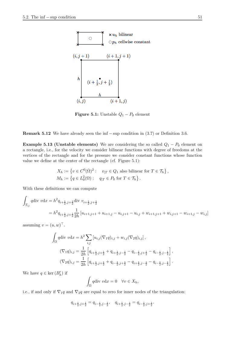
Figure 5.1: Unstable Q1 − P0 element
Remark 5.12 We have already seen the inf − sup condition in (3.7) or Definition 3.6.
Example 5.13 (Unstable elements) We are considering the so called Q1 − P0 element ona rectangle, i.e., for the velocity we consider bilinear functions with degree of freedoms at thevertices of the rectangle and for the pressure we consider constant functions whose functionvalue we define at the center of the rectangle (cf. Figure 5.1):
Xh :=v ∈ C0(Ω)2 : v|T ∈ Q1 also bilinear for T ∈ Th
,
Mh :=q ∈ L2
0(Ω) : q|T ∈ P0 for T ∈ Th.
With these definitions we can compute
∫
Tij
qdiv vdx = h2qi+ 1
2,j+ 1
2
div vi+ 1
2,j+ 1
2
= h2qi+ 1
2,j+ 1
2
1
2h[ui+1,j+1 + ui+1,j − ui,j+1 − ui,j + wi+1,j+1 + wi,j+1 − wi+1,j − wi,j]
assuming v = (u,w)⊤.
∫
Ωqdiv vdx = h2
∑
i,j
[ui,j(∇1q)i,j + wi,j(∇2q)i,j] ,
(∇1q)i,j =1
2h
[
qi+ 1
2,j+ 1
2
+ qi+ 1
2,j− 1
2
− qi− 1
2,j+ 1
2
− qi− 1
2,j− 1
2
]
,
(∇2q)i,j =1
2h
[
qi+ 1
2,j+ 1
2
+ qi− 1
2,j+ 1
2
− qi+ 1
2,j− 1
2
− qi− 1
2,j− 1
2
]
.
We have q ∈ ker (B′h) if
∫
Ωqdiv vdx = 0 ∀v ∈ Xh,
i.e., if and only if ∇1q and ∇2q are equal to zero for inner nodes of the triangulation:
qi+ 1
2,j+ 1
2
= qi− 1
2,j− 1
2
, qi+ 1
2,j− 1
2
= qi− 1
2,j+ 1
2
.

52 Chapter 5: Saddle-point problem
Figure 5.2: Pressure instability in L-shaped domain
A possible setup for these equations is to assume
qi+ 1
2,j+ 1
2
=
a for i+ j = 2k
b for i+ j = 2k + 1, k ∈ N,
cf. Figure 5.2.
Theorem 5.14 (Fortin Criterion) Let b : X × M → R a bilinear form which fulfils theinf − sup condition. Let Xh ⊂ X and Mh ⊂M be finite-dimensional subspaces. Let Πh : X →Xh be a linear and bounded operator, such that
b(v −Πhv, µh) = 0 ∀µh ∈Mh.
If ‖Πh‖ ≤ C where C is independent from h, then (Xh,Mh) is a stable finite element space.
Proof
β ‖µh‖ ≤ supv∈X
b(v, µh)
‖v‖
= supv∈X
b(Πhv, µh)
‖v‖
≤ C supv∈X
b(Πhv, µh)
‖Πhv‖
= Cb(vh, µh)
‖vh‖.
Example 5.15 (MINI element) The space for the velocity is defined as
M10,0 :=
vh ∈ C(Ω) ∩H10 (Ω)
d : vh|T ∈ P1 for T ∈ Th2
plus a bubble function, e.g.,b(x) = λ1λ2λ3
in barycentric representation, i.e.
Xh := M10,0
⊕
B3,

5.2. The inf − sup condition 53
Figure 5.3: MINI Element
where B3 corresponds to the space spanned by the bubble function
B3 :=v ∈ C0(Ω) : v|T ∈ spanλ1λ2λ3 for T ∈ Th
.
The space for the pressure is defined as
Mh :=
qh ∈ C(Ω) ∩ L20(Ω) : qh|T ∈ P1 for T ∈ Th
.
Lemma 5.16 (MINI element) Let Ω be convex and ∂Ω smooth enough. Then the MINIelement (Xh,Mh) is stable.
Proof We define the projectorΠ0
h : H10 (Ω) → M1
0,0
by means of the solution of the Helmholtz equation:
(∇(Π0
hv),∇w
)
0+(Π0
hv, q)
0= (∇v,w)0 + (v,w)0 ∀w ∈ M1
0,0.
Obviously,∥∥Π0
hv∥∥1≤ ‖v‖1 ,
∥∥Π0
hv − v∥∥0≤ C1h
∥∥Π0
hv − v∥∥1≤ C2h ‖v‖1 .
Further, we define Π1h : L2(Ω) → B3 by
∫
T
(Π1
hv − v)dx = 0 ∀T ∈ Th.
One can easily show that∥∥Π1
hv∥∥0≤ C3 ‖v‖0. Let
Πhv := Π0hv +Π1
h
(v −Π0
hv).
Obviously, ∫
T
(Πhv − v) dx = 0 ∀T ∈ Th.
Further,
b(v −Πhv, qh) =
∫
Ωdiv (v −Πhv)qhdx
=
∫
∂Ω(v −Πhv)nqhdS −
∫
Ω(v −Πhv)∇qhdx
= 0 ∀qh ∈Mh.

54 Chapter 5: Saddle-point problem
Additionally,
‖Πhv‖1 ≤∥∥Π0
hv∥∥1+ C4h
−1∥∥Π1
h(v −Π0hv)∥∥0
≤ C2 ‖v‖1 + C4h−1C3
∥∥v −Π0
hv∥∥0
≤ C2 ‖v‖1 + C4C3C2 ‖v‖1 .

55
6 A posteriori error estimation
6.1 Introduction
Find u ∈ H10 (Ω) such that
(∇u,∇ϕ) = (f, ϕ) ∀ϕ ∈ H10 (Ω).
The corresponding discrete problem reads: Find uh ∈ Vh ⊂ H10 (Ω) such that
(∇uh,∇ϕ) = (f, ϕ) ∀ϕ ∈ Vh.
We want to know or at least estimate the error
‖u− uh‖ .
Of course, the concrete error depends on the considered norm. We know, for example, that
‖u− uh‖1 ≤C
αinfv∈Vh
‖u− v‖1 ≤C
α‖u− Ihu‖1 ≤ C(u, uh)
due to Céa’s lemma (and interpolation error estimation as well as the assumption of C2 reg-ularity). Is this an a priori or an a posteriori error estimation? This is an a priori errorestimation because we estimate the error with the unknown function u. An estimation of theform
‖u− uh‖ ≤ C(uh)
is called an a posteriori error estimation because we estimate the error with the known discretesolution.
6.2 Residual based error estimator
We consider the Laplace equation in the following form:
−∆u = f in Ω
u = 0 on ∂Ω.
The variational formulation reads: Find u ∈ H10 (Ω) or uh ∈ Vh ⊂ H1
0 (Ω) such that
(∇u,∇ϕ) = (f, ϕ) ∀ϕ ∈ H10 (Ω),
(∇uh,∇ϕ) = (f, ϕ) ∀ϕ ∈ Vh.
We now define a goal functional J(u) (e.g., J(u) := u(xNumPDE3) if we want to know thefunction value at a specific point) and define the error as
eh := J(u)− J(uh).

56 Chapter 6: A posteriori error estimation
In order to compute the error with respect to this goal functional, we consider an additionalproblem called dual problem: Find z ∈ H1
0 (Ω) such that
(∇z,∇ϕ) = (J(u), ϕ) ∀ϕ ∈ H10 (Ω).
The discrete dual problem then reads: Find zh ∈ Vh such that
(∇zh,∇ϕ) = (J(u), ϕ) ∀ϕ ∈ Vh.
The function z is called weight function. In the case of Poisson’s equation it is in fact Green’sfunction. The weight function is a measure for the sensitivity of the solution u of the primalproblem with respect to the goal functional.
Lemma 6.1J(u)− J(uh) = (∇u,∇ (z − Ihz)) + h.o.t.
where h.o.t. denotes higher order terms of the order O(hk), k ≥ 2.
J(u)− J(uh) ≤ (∇uh,∇ (z − Ihz))
≤
∫
Ω∇uh · ∇ (z − Ihz) dx
≤∑
T∈Th
∣∣∣∣
∫
T
∇uh · ∇ (z − Ihz) dx
∣∣∣∣
≤∑
T∈Th
∣∣∣∣
∫
T
(−∆uh, z − Ihz) dx
∣∣∣∣+ |⌊∇uh⌋∂T | |⌊z − Ihz⌋∂T |
This estimation enables us to develop a refinement strategy : Cells T with "large" contributionto the error estimation are refined, whereas cells with "small" contribution are kept.
We define the following measures in order to estimate the local error in the discrete solution:
RT := RT (uh) := ∆uh + f for T ∈ Th (cell error),
Re := Re(uh) := ⌈∂nuh⌉e for e ∈ Γh (jump error),
where
⌈∂nuh⌉e := −(∇uh,TnT +∇uh,T ′nT ′
)
= −(∇uh,TnT −∇uh,T ′nT
)
=(∇uh,T ′ −∇uh,T
)nT
and T ′ denotes the neighbouring cell of T adjacent to edge e. Re is a measure for the disconti-nuity of the gradient of the discrete solution between two neighbouring cells.
Excurse Goal: Solve the linear system Ax = b, A ∈ Rn×n, b ∈ R
n. Assume that xk is anapproximation of x.
A(x− xk) = b−Axk.
Let rk = b − Axk be the residual and ek = x − xk the error. Then the above equation isequivalent to
⇔ Aek = rk
⇔ ek = A−1rk (assuming regularity of A)
⇒ ‖ek‖ ≤∥∥A−1
∥∥ ‖rk‖ .

6.2. Residual based error estimator 57
PICTURES!!!
Figure 6.1: Error contributions
The goal of a posteriori error estimators is to give a computable approximation of∥∥A−1
∥∥.
ωT :=T ′ ∈ Th : T and T ′ have a common edge or T = T ′
,
ωe :=T ′ ∈ Th : e ⊂ ∂T ′
.
6.2.1 Residual estimators
These estimators were first developed by Babuška & Rheinhold [1978].
We consider the local expression
ηT,R :=
h2T ‖RT ‖20,T +
1
2
∑
e∈∂T
he ‖Re‖20,e
1
2
for T ∈ Th.
Based on this local description of the error, we define the global estimator
ηR :=
∑
T∈Th
‖RT ‖20,T +
∑
e∈Γh
he ‖Re‖20,e
1
2
.
Theorem 6.2 Let Th be a quasiuniform triangulation. Then a constant C = C(Ω, κ) existssuch that
‖u− uh‖1,Ω ≤ C
∑
T∈Th
η2T,R
1
2
and
ηT,R ≤ C
‖u− uh‖
21,ωT
+∑
T ′∈ωT
h2T ′ ‖f − fh‖20,T ′
1
2
for all T ∈ Th.
Proof Duality argument:
|u− uh|1 ≤ supw∈H1
0(Ω),|w|
1=1
(∇(u− uh),∇w)0
and
(∇(u− uh),∇vh) = 0 ∀vh ∈ Sh,
i.e., Galerkin orthogonality.
We define the functional
l : H10 (Ω) → R

58 Chapter 6: A posteriori error estimation
by means of
〈l, w〉 := (∇(u− uh),∇w)0,Ω
= (f,w)0,Ω −∑
T
(∇uh,∇w)0,T
= (f,w)0,Ω −∑
T
(−∆uh, w)0,T +∑
e⊂∂T
(∇uh · n, w)0,e
=∑
T
(∆uh + f,w)0,T +∑
e∈Γh
(⌈∂nuh⌉, w)0,e
=∑
T
(RT , w)0,T +∑
e∈Γh
(Re, w)0,e .
Considering the Interpolation operator of Clément (see Numerik PDE) we may write
‖w − Ihw‖0,T ≤ ChT ‖∇w‖0,ωTfor T ∈ Th,
‖w − Ihw‖0,e ≤ Ch1
2e ‖∇w‖0,ωe
for e ∈ γh
and
〈l, w〉 = 〈l, w − Ihw〉
≤∑
T
‖RT ‖ ‖w − Ihw‖0,T +∑
e∈Γh
‖Re‖0,e ‖w − Ihw‖0,e
≤ C∑
T
hT ‖RT ‖0,T |w|1,ωT+C
∑
e∈Γh
h1
2e ‖Re‖0,e |w|1,ωe
≤ C∑
T
ηT,R |w|1,T
≤ CηR |w|1,Ω .
Now the use of the duality argument yields the inequalities.
6.2.2 Dual weighted Residual method (DWR)
Assume a linear (goal) functional J(·) : V → R. We are interested in controlling the error
J(eh) = J(u)− J(uh).
In this context, we consider the dual problem: Find z ∈ V (= H10 (Ω)) such that
(∇z,∇ϕ) = J(ϕ) ∀ϕ ∈ V.
Consider the error
J(eh) = (∇eh,∇z) = (∇eh,∇ (z − ψh)) ∀ψh ∈ Vh.
It follows that
J(eh) =∑
T∈Th
− (∆eh, z − ψh)T + (∂neh, z − ψh)∂T
=∑
T∈Th
f +∆uh︸ ︷︷ ︸
Residual
, z − ψh
T
− (∂nuh, z − ψh)∂T
=∑
T∈Th
(f +∆uh, z − ψh)T −1
2(⌈∂nuh⌉, z − ψh)∂T
.

6.2. Residual based error estimator 59
PICTURE!!!
Figure 6.2: Superconvergence
We have
|J(eh)| ≤∑
T∈Th
∣∣∣∣(f +∆uh, z − ψh)T −
1
2(⌈∂nuh⌉, z − ψh)∂T
∣∣∣∣.
Considering the Hölder inequality
|J(eh)| ≤∑
T∈Th
‖f +∆uh‖T︸ ︷︷ ︸
=:ρT (uh)
‖z − Ihz‖T︸ ︷︷ ︸
=:ωT (z)
+1
2‖⌈∂nuh⌉‖∂T\∂Ω ‖z − Ihz‖∂T
≤∑
T∈Th
ρT (uh)ωT (z) + ρ∂T (uh)ω∂T (z) ,
where
ρ∂T (uh) :=1
2h− 1
2
T ‖⌈∂nuh⌉‖∂T\∂Ω ,
ω∂T (z) := h1
2
T ‖z − Ihz‖∂T .
The exact solution z to the dual problem is unknown, so we need a possibility to compute theerror in the dual solution. Some ideas might be:
1. Take an approximation: Find zh ∈ Vh such that
(∇zh,∇ϕ) = J(ϕ) ∀ϕ ∈ Vh.
This is a bad idea, because the interpolation of the approximation is identical with theapproximation itself so the "’error"’ in the dual solution will be always zero and thereforethe error estimator will always give the value zero.
2. A priori error estimation for z:
‖z − Ihz‖T ≤ Ch∥∥∇2z
∥∥T.
In this case the second derivative of z is not known. It possible to assume that this secondderivative is constant and take Ch as an "’estimation"’ for the dual solution but in factthe information of the dual solution is completely lost. Also bad idea!
3. Take an approximation in a larger space: Find zh2
∈ Vh2
such that
(
∇zh2
,∇ϕ)
= J(ϕ) ∀ϕ ∈ Vh2
.
This is possible but increases the computational costs extremely! To lower the computa-tional costs the refinement h→ h
2 is often done only locally.
4. Trick for higher derivatives: Locally refinement of the grid leads to superconvergence:Convergence order increases from h2 to h
5
2 .

60 Chapter 6: A posteriori error estimation
6.3 Exact grid optimization
Optimization problem 1 Let
• N : number of cells
• η: error estimator
minN such that η ≤ TOL
with some tolerance TOL.
Optimization problem 2 Let
• N : number of cells
• η: error estimator
min η such that N ≤ Nmax
with some maximum number of cells Nmax.
We can have the following view:
h−1T ρT (uh) = h−1
T ‖f +∆uh‖T +1
2h− 3
2
T
∥∥h−1
T ⌈∂nuh⌉∥∥∂T\∂Ω
→ φu(xT )
h−3T ωT (zh) = max
h−3T ‖z − Ihz‖T , h
− 5
2
T ‖z − Ihz‖∂T
→ ψz(xT )
Let A(x) = φ(x)ψ(x).
∑
T∈Th
ρT (uh)ωT (zh) =∑
T∈Th
h4Th−4T ρT (uh)ωT (zh)
≈
∫
Ωh2(x)A(x)dx.
N =∑
T∈Th
1
=∑
T∈Th
h2Th−2T
≈
∫
Ωh−2(x)dx.
So the optimization problem reads:
minF (h) :=
∫
Ωh2(x)A(x)dx such that N(h) :=
∫
Ωh−2(x)dx = Nmax.
The Lagrange functional is
L(h, λ) := F (h) + λ(N(h)−Nmax).
It holds
dtL(h+ tϕ, λ+ tµ)|t=0 = 0.

61
7 Practical aspects
7.1 Solution of the discrete Stokes problems
We only consider finite element discretizations which fulfil (3.7). With the usual nodal basisfunctions of the spaces Xh ⊂ X and Qh ⊂ Q the discrete system can be written in block matrixform as
Aξ =
(A B
−B⊤ 0
)(xy
)
=
(b0
)
=: β, (7.1)
where ξ := (x, y)⊤ denotes the vector of nodal values of the representations
vh =
NX∑
i=1
xiψih, ph =
NQ∑
i=1
yiχih,
and the corresponding matrices and right hand sides
A :=((
∇ψjh,∇ψ
ih
))NX
i,j=1, B := −
((
χjh,div ψ
ih
))NX ,NQ
i,j=1, b :=
((f, ψi
h
))NX
i=1.
What possibilities do we have to solve the system Aξ = β?
1. Apply our known methods to solve linear systems directly to A, e.g., LU decomposition,CG, GMRES or multigrid methods.
a) Advantages:
i. We can reuse our existing implementations of these methods.
ii. A is known to be regular due to the assumption (3.7).
b) Disadvantages:
i. What is the condition number of A? The condition number of A is of the orderO(h−2
)but what about the block system with the contributions of B?
ii. The memory consumption is higher compared to storing A and B separately. IfB cannot be transposed with low computational costs, it is beneficial, to storeadditionally −B⊤. In every case, the "0" does not need to be stored in memory.
2. Are there methods which only need methods to efficiently invert A, i.e., solve linearsystems with the system matrix A, and multiplications with B (and maybe −B⊤)? Theanswer to this question is yes and we will discuss several possibilities in the next section.

62 Chapter 7: Practical aspects
7.1.1 Schur complement method
Let
Aξ =
(A BC D
)(xy
)
=
(fg
)
be a linear system in block matrix form. Assume that A is regular. Then the first block canbe solved for x and the result inserted into the second block which yields
x = A−1f −A−1By(D − CA−1B
)y = g − CA−1f.
The matrix Σ := D−CA−1B is called the Schur complement of A in the block matrix A. Withthis notion of Σ, A can be decomposed in block triangular matrices:
A =
(A BC D
)
=
(A 0C D −CA−1B
)
·
(I A−1B0 I
)
.
In case of the Stokes system, the above results reduce to
x = A−1b−A−1By,
B⊤A−1By = B⊤A−1b,
Σ = B⊤A−1B,
A =
(A B
−B⊤ 0
)
=
(A 0
−B⊤ Σ
)
·
(I A−1B0 I
)
.
7.1.1.1 Uzawa algorithm
The "classical" method to solve the saddle-point problem (7.1) is the Uzawa algorithm:
Algorithm 7.1 (Uzawa) Given an initial value y0. For l ∈ N compute:
1.
Axl = b−Byl−1
2.
yl = yl−1 + θB⊤xl
Until convergence is reached.
Here, θ > 0 denotes a relaxation parameter which needs to be chosen appropriately. Theiteration is done in the space of the nodal values of the pressure component. To balance possibleirregularities of the computational grid Th (anisotropic cells, heterogeneous grid spacing), it isadvisable to precondition the system with the mass matrix of the trial space of the pressure,
M :=MQ =((
χjh, χ
ih
))NQ
i,j=1.
This leads to the so called modified Uzawa algorithm:
Algorithm 7.2 (Uzawa (modified)) Given an initial value y0. For l ∈ N compute:

7.1. Solution of the discrete Stokes problems 63
1.
Axl = b−Byl−1
2.
Myl =Myl−1 + θB⊤xl
Until convergence is reached.
Each iteration requires to invert the stiffness matrix A as the most costly operation. Fur-thermore, the mass matrix M needs to be inverted. Both can be accomplished in an efficientway with, e.g., the (preconditioned) CG or multigrid algorithms. By eliminating xl (insertingthe first step into the second one), we obtain the Uzawa algorithm in form of a fixed pointiteration:
yl =(I − θlM
−1Σ)yl−1 + θlM
−1B⊤A−1b. (7.2)
Therefore, the Uzawa algorithm is a damped Richardson iteration for solving the Schur comple-ment equation. It holds the following result which is obtained by the application of Banach’sfixed point theorem:
Theorem 7.3 (Uzawa algorithm) Assume that the condition
θl ≤1− q
‖M−1Σ‖, q ∈ (0, 1) (7.3)
holds. Then Uzawa’s algorithm converges to the solution (x, y) of the saddle-point problem(7.1). Furthermore, we have the following estimate on the error:
∥∥∥yl − y
∥∥∥ ≤
ql
1− q
∥∥y0 − y
∥∥ .
Proof The exact solution y fulfils the fixed point equation
y =(I − θlM
−1Σ)y + θlM
−1B⊤A−1b.
Substracting (7.2) yields the following estimate on the error el := y − yl:
∥∥∥el∥∥∥ ≤
∥∥I − θlM
−1Σ∥∥ ·∥∥∥el−1
∥∥∥ .
This implies∥∥∥el∥∥∥ ≤
∣∣1− θl
∥∥M−1Σ
∥∥∣∣ ·∥∥∥el−1
∥∥∥
(7.3)
≤ q∥∥∥el−1
∥∥∥ .
The Theorem now follows by the application of Banach’s fixed point theorem.
Remark 7.4 1. It can be shown, that∥∥M−1Σ
∥∥ is uniform for all grid spacings h. Therefore,
the Uzawa algorithm converges with an order that is independent of h, if we additionallyassume, that θl is small enough.
2. The rate of convergence can be optimized by choosing θl variable in each iteration. Thenthe Uzawa algorithm corresponds to the method of steepest descent for solving the Schurcomplement equation. We omit the detailed discussing and directly proceed to the moreefficient CG method.
64 Chapter 7: Practical aspects
7.1.1.2 Conjugate gradient (CG) method
Similarly to the modified Uzawa algorithm, the system is preconditioned by the pressure massmatrix MQ, i.e.: The CG method is applied as preconditioned CG (PCG) method to the mod-ified system
M−1Σy =M−1B⊤A−1b.
This is equivalent to the application of the CG algorithm to symmetric and (up to mean valuecomputation) positive definite matrix
M− 1
2ΣM− 1
2 .
The spectral condition number
κ :=λmax
(M−1Σ
)
λmin (M−1Σ)
determines the rate of convergence according to
∥∥∥yl − y
∥∥∥ ≤ κ
(
1− κ−1
2
1 + κ−1
2
)l∥∥y0 − y
∥∥ , l ∈ N,
where y0 is the initial guess of the iteration.
Theorem 7.5 (Schur complement) The following estimate holds for the Schur complementΣ = B⊤A−1B:
κ(M−1Σ
)≤ c−1
0 β−2,
where β > 0 denotes the constant from (3.7) of the used finite element discretization Xh/Qh.In the conforming case Xh ⊂ X it holds c0 = 1 and c0 = 4 in the general case.
Proof Cf., e.g., [10].
The saddle-point problem (7.1) can also be solved by a multigrid algorithm. In this case, specialattention has to be paid to the smoother. We will discuss that aspect in the context of themore general situation of the linearized Navier-Stokes equations.
7.2 Solution of the stationary Navier-Stokes equations
The solution of the nonlinear Navier-Stokes equations necessitates the application of an iterativemethod, e.g., Newton or Richardson iterations. In the case of dominating nonlinearities, i.e.,dominance of the convective terms (and therefore high Reynolds numbers), some critical aspectsneed to be considered and respected.
7.2.1 Discretization of the convective terms
Consider the stationary Navier-Stokes equations in dimensionless form
−ν∆v+ (v · ∇)v +∇p = f
div v = 0

7.2. Solution of the stationary Navier-Stokes equations 65
PICTURE!!!
Figure 7.1: Solution of one-dimensional model problem
on some domain Ω ⊂ Rd, (d = 2, 3) with sufficiently smooth boundary ∂Ω. For the sake of
simplicity, we restrict the following discussion to the case of homogeneous Dirichlet boundaryconditions on the whole boundary ∂Ω.
If we apply a conforming finite element discretization which fulfils (3.7), the variational formu-lation yields the following discrete contribution of the convective term:
((v · ∇)v, ψ) ≈ ((vh · ∇)vh, ψh) .
This term mainly contributes to the off-diagonals of the system matrix, which consequentlylooses its definiteness. On coarser grids, this leads in turn to non-physical oscillations in thesolution as well as the breakdown of the classical iterative solution methods, e.g., Jacobi, Gauß-Seidel or SOR algorithms.
7.2.1.1 Stabilization in the one-dimensional case
We illustrate these statements for the case of a simple one-dimensional model. On Ω = I :=(0, 1) ⊂ R we consider the boundary value problem
−εu′′(x) + q(x)u′(x) = 0, x ∈ I, u(0) = 1, u(1) = 0
(Sturm-Liouville problem). We assume, that q(x) ≡ 1 on I. Then the unique solution reads
uε(x) =e
1
ε − exε
e1
ε − 1.
In the case ε≪ 1 it holds for x = 1− δ and δ > ε
uε(1− δ) =e
1
ε
1ε− 1
(
1− e−δε
)
≈ 1, supx∈I
∣∣uε′′(x)
∣∣ ≈ ε−2,
which justifies the term boundary layer . For ε = 0 we obtain the solution u0 ≡ 1, whichobviously does not fulfil the boundary condition on the right boundary x = 1.
The approximation of this problem with the usual (centralized) difference scheme and anequidistant grid spacing h = 1
N+1
−u′′(x) ≈1
h2(−yn−1 + 2yn − yn+1) (2nd order accurate),
u′(x) ≈1
2h(yn+1 − yn−1) (2nd order accurate),
yields
−
(
ε+h
2
)
yn−1 + 2εyn −
(
ε−h
2
)
yn+1 = 0, 1 ≤ n ≤ N, y0 = 1, yN+1 = 0.
The resulting coefficient matrix is consequently only diagonally dominant under the restrictivecondition
h ≤ 2ε.

66 Chapter 7: Practical aspects
For h > 2ε the discrete solution incorporates non-physical oscillations. To verify this statement,we make the following trial for the solution:
yn = λn.
The possible values for λ are the roots of the quadratic equation
λ2 +2ε
h2 − ε
λ−h2 + εh2 − ε
= 0.
Therefore, the solution has the general form
yn = c+λn+ + c−λ
n−.
Considering the boundary conditions y0 = 1 and yN+1 = 0 yields the solution
yn =λN+1+ λn− − λN+1
− λn+
λN+1+ − λN+1
−
, n = 0, . . . , N + 1.
In our case, the roots are given by
λ+ = 1, λ1 =ε+ h
2
ε− h2
.
For ε≪ h2 it holds λ− ≈ −1. In this case, we obtain an oscillating solution:
yn =λn− − λN+1
−
1− λN+1−
, n = 0, . . . , N + 1,
which does not reflect the correct solution. There are different strategies to omit this defectwhich we depict in the following:
1. Upwind discretization: Instead of using the central difference quotient for the approx-imation of the first derivative of u, we can chose one of the one-sided quotients
∆+h u(x) =
u(x+ h)− u(x)
h, ∆−
h u(x) =u(x)− u(x− h)
h.
If we chose the backward or upwind difference quotient ∆−h , we respect the physical
phenomenon of information transport in positive x direction. The difference equationsread
(−ε+ h)yn−1 + (2ε+ h)yn − εyn+1 = 0
and the resulting system matrix is diagonally dominant for arbitrary h > 0. The trialyn = λn for the solution yields the roots
λ+ =ε+ h
ε, λ− = −1.
The critical root is λ+ > 0 in this case and the discrete solution
yn =λN+1+ − λn+
λN+1+ − 1
does not incorporate non-physical oscillations.
The one-sided difference quotient is only first order accurate, i.e., O(h), and, therefore,the overall algorithm is only first order accurate. This limits the precision of the ap-proximation in regions where the solution is smooth, even if the grid spacing h is chosensufficiently small according to h ≈ ε in the boundary layer.

7.2. Solution of the stationary Navier-Stokes equations 67
2. Artificial diffusion: We discretize the first drivative u′(x) with the central differencequotient and set the diffusion coefficient to a larger value εh := ε+ δh. This is a changein the physics of the modelled problem!!! In case of our model problem with q ≡ 1, themodified discretization is stable if we chose δ ≥ 1
2 . But the boundary layer is significantlysmeared over to the interval [1 − εh, 1] and the global accuracy of the approximation isonly O(h) due to the perturbation of the differential operator.
We have seen at the hand of this simple example that the damping strategies upwind discretiza-tion and artificial diffusion lead on the one hand to stable discretizations but on the other handthe order of the approximation is reduced to O(h). Consequently, the question about higherorder stabilization schemes for the discretization of transport terms is not answered in a satis-factory manner yet. Approaches in this direction use higher order one-sided difference quotient(in the case of upwinding) or artificial diffusion terms of the form δh2u(iv). But the strong Mmatrix property can only be achieved with discretizations of first order. This restriction canbe circumvented by a modification of the artificial diffusion in the context of Galerkin methodswith finite element discretizations.
3. Streamline diffusion: We consider the special case q ≡ 1. This method modifies theusual variational formulation
ε(u′, ϕ′
)+(u′ + αu,ϕ
)= (f, ϕ) , ∀ϕ ∈ H := H1
0 (I),
with some α ≥ 0, to
ε(u′, ϕ′
)+(u′ + αu,ϕ+ δϕ′
)=(f, ϕ+ δϕ′
), ∀ϕ ∈ H := H1
0 (I),
where δ denotes a parameter function which depends on the grid parameter h. Theresulting bilinear form
aδ(u, v) := ε(u′, v′
)+(u′ + αu,ϕ+ δϕ′
)
is coercive,aδ(v, v) ≥ ‖v‖2δ , v ∈ H,
with respect to the modified energy norm
‖v‖δ :=
(
ε∥∥v′∥∥2 +
∥∥∥δ
1
2 v′∥∥∥
2+ α ‖v‖2
) 1
2
.
We want to emphasize that, in general, the parameter δ is a function of x (piecewiseconstant on the triangulation 0 = x0 < . . . < xN+1 = 1) and, therefore, has to be
considered within the norm∥∥∥δ
1
2 v′∥∥∥. Then, the corresponding finite-element-Galerkin
method (with linear trial functions) in the trial space Hh ⊂ H reads
Find uh ∈ Hh : aδ(uh, ϕh) = lδ(ϕh) ∀ϕh ∈ Hh,
with the modified right hand side
lδ(v) :=(f, v + δv′
).
It can be shown that, in the case of a smooth solution u (without boundary layer) or ifthe grid spacing in the boundary layer is sufficiently small, the order of the approximation
with respect to the energy norm is O(
h3
2
)
. Consequently, the simplest finite element
method with streamline diffusion has a higher order than the upwinding-stabilized finitedifference method.

68 Chapter 7: Practical aspects
7.2.1.2 Stabilization of the Navier-Stokes equations
The methods for the stabilization of the transport terms that we described for the one-dimensional case can be generalized to the multi-dimensional Navier-Stokes equations.
1. Upwind stabilization: It is possible to transfer the idea of the upwind stabilizationfrom one-dimensional finite differences to multi-dimensional finite element methods. Theconstruction is technically quite involved because we need to determine the upwind di-rection or, more precisely, the "upwind area". We do not discuss this technique in detailhere and refer the interested reader to [10].
2. Artificial diffusion: This approach works analogously to the one-dimensional case andincorporates the same limitations, especially the modification of the underlying physics.
3. Streamline diffusion/Residual based stabilization: The basic idea of streamlinediffusion is to introduce artificial diffusion only in the direction of transport or in thedirection of streamlines, respectively, such that the full second order of the discretizationis preserved. There is a general construction principle behind this approach which we willdiscuss after a simple example.
We describe a simple variant for the stationary Navier-Stokes equations: Find vh ∈ Xh
and ph ∈ Qh such that
((vh · ∇)vh, ϕh) + ν (∇vh,∇ϕh)− (ph,div ϕh) + sh (vh, ph , ϕh, χh)
= (f, ϕh) + rh (vh, ph , ϕh, χh)
holds for all tuples ϕh, χh ∈ Xh ×Qh, where
sh (vh, ph , ϕh, χh) =∑
T∈Th
δT (∇ph + (vh · ∇)vh,∇χh + vh∇ϕh)T + (div vh,div ϕh)T ,
rh (vh, ph , ϕh, χh) =∑
T∈Th
δT (f + ν∆vh,∇χh + vh∇ϕh)T
with some reference velocity vh. The stabilization parameters δT are chosen according to
δT = min
h2Tν,hT‖vh‖
.
This choice of the stabilization has several special properties:
a) (∇ph,∇χh)T : Stabilizes the pressure for the conforming Q1/Q1 element such that(3.7) is fulfilled (with a modified numerator).
b) ((vh · ∇)vh, vh∇ϕh)T : Stabilizes the transport operator (streamline diffusion).
c) (div vh,div ϕh)T : Improves/stabilizes the conservation of mass (incompressibility).
The other terms are only needed in order to preserve the second order accuracy of thediscretization. A theoretical analysis shows that this kind of stabilization in the contextof a Galerkin methods leads in fact to an improvement over the upwind stabilization: the
discretization error on the Q1/Q1 element converges with O(
h3
2
)
.
General construction principle: The general principle behind the streamline diffusionmethod are the residual based stabilization methods. To motivate this approach, consider

7.2. Solution of the stationary Navier-Stokes equations 69
a linear differential operator L and some right hand side function f . We rewrite the taskof finding a solution u of the equation
Lu = f
in form of a minimization problem: Find u such that
u = argminv ‖Lv − f‖2 .
It can be shown that this is equivalent to compute u as the solution of the variationalequation
(Lu− f, Lϕ) = 0 ∀ϕ,
where u, ϕ are elements of some appropriate function space. This Galerkin method isknown as Galerkin-least squares (GLS) method . Let us consider the last equation in theform
(Lu,Lϕ) = (f, Lϕ) ∀ϕ.
The bilinear form
aGLS(u, v) := (Lu,Lv)
is always symmetric and coercive which means that the matrix resulting from a finiteelement discretization is always symmetric and positive definite. This sounds like the"ideal" variational formulation but it has two severe disadvantages:
a) If L is a differential operator of the order k ∈ N, we need to construct finite elementswhich are Hk conform. In the case k = 1 we can simply use our standard Lagrangefinite element, but even for a second order differential operator like L = −∆ we needfinite elements with higher global regularity. The construction of such elements isnot trivial at all!
b) The matrix resulting from the bilinear form
aGLS(u, v) := (Lu,Lv)
has a condition number that is squared compared to the "standard" variationalformulation resulting from the approach
(Lu,ϕ) .
Due to these reasons, it is not advisable to use this kind of variational formulation forthe discretization of a PDE except in very special or hard cases. But we can use thisformulation elementwise for the stabilization of our discretization based on the "usual"variational formulation: Let R(u) := Lu− f denote the residual of our PDE under con-sideration and a(·, ·) the bilinear form associated with L. Then the stabilized formulationreads: Find uh such that
a(uh, ϕh)− (f, ϕ) +∑
T∈Th
(R(uh), δTLϕh)T = 0 ∀ϕh.
This is known as Galerkin-least squares stabilization. The advantage of the formulationis that it is strictly consistent with our PDE because the exact solution u fulfils thisequations.

70 Chapter 7: Practical aspects
The evaluation of the the operator Lϕh can be computationally expensive. So it is possibleto generalize the GLS stabilization to the form
a(uh, ϕh)− (f, ϕ) +∑
T∈Th
(R(uh), δTWϕh)T = 0 ∀ϕh
with some weighting operator W . Two common choices in the context of convection-dominated problems are
• W = L: GLS stabilization
• W = vh∇ϕh: The streamline-upwind Petrov-Galerkin (SUPG) stabilization opera-tor.
In the case of a nonlinear operator N(u), the weighting operator W is chosen as a lin-earization of N which incorporates the features that need to be stabilized.
So, the above simple variant of a residual based stabilization uses the GLS stabilizationfor the continuity equation and the operator
∇χh + vh∇ϕh
for the stabilization of the momentum equation which is the sum of pressure stabilizationand SUPG stabilization.
Remark 7.6 The operator W can be interpreted as considering the contained parts ofthe differential operator L in a GLS manner because the part
(W (uh), δTWϕh)T
of the "full" stabilization operator
(R(uh), δTWϕh)T
is a GLS formulation for W .
4. Local projection stabilization: Streamline diffusion has significant disadvantages froma practical point of view. Its usage in conjunction with a Neumann outflow boundarycondition ("do nothing" boundary condition) in channel flows leads to a non-physical flowbehaviour ("numerical" boundary layer) at the outflow boundary: streamlines are flexedoutwards. Furthermore, the evaluation of the additional terms can become expensive,especially in three-dimensional flow problems.
These problems can be avoided by the application of the so called local projection stabi-lization. Here, the stabilization forms rh = 0 and
sh := (∇ (ph − π2hph), δh∇ (χh − π2hχh))+((vh · ∇) (vh − π2hvh), δh (v · ∇) (ϕh − π2hϕh))
are used. π2h is a projection or interpolation to the trial space L2h which is defined on acoarser triangulation T2h. The resulting method is of second order, the evaluation of thecorresponding system matrices relatively cheap and the error in consistency at an outflowboundary is avoided. Again, the parameter δh is chosen cellwise in dependence on thelocal convection and diffusion.
5. Discontinuous Galerkin (DG) method: The application of a discontinuous Galerkindiscretization instead of a "standard" continuous Galerkin method has also a stabilizingeffect but is not discussed here. We refer the interested reader to the literature.

7.2. Solution of the stationary Navier-Stokes equations 71
7.2.2 Linearization
As we have already mentioned above, we need to linearize the nonlinear Navier-Stokes equationsin order to obtain a discrete solution with the Newton or Richardson iterative methods, forexample. We describe the various linearization techniques on the continuous level. Startingwith some initial value v
0 ∈ X we determine a series of iteratesvl, pl∈ X × Q for l ∈ N
which converges to the exact solution v, p.
7.2.2.1 Stokes linearization
In the case of small Reynolds numbers
Re =1
ν≪ 1
(viscous liquids, small velocities, small geometrical dimensions), the simple Stokes lineariza-tion
−ν∆vl +∇pl = f −
(vl−1 · ∇
)vl−1
div vl = 0
is often sufficient. The nonlinearity (v · ∇)v is treated fully explicit and in each iteration thesymmetric and positive definite Stokes operator has to be inverted.
7.2.2.2 Oseen linearization
If the Reynolds numbers are larger, the so called Oseen linearization is used:
−ν∆vl + (v · ∇)vl +∇pl = f
div vl = 0
.
Here, v ≈ vl is an appropriate approximation, e.g., in the simplest case v := v
l−1 (constant ex-trapolation), but also higher order approximations are possible (e.g., with linear extrapolation).The operator which has to be inverted in each iteration is a non-symmetric convection-diffusionoperator. In order to improve the convergence, this functional iteration should be done in formof a defect correction iteration: A correction is computed with the defect
dl−1 := f − ν∆vl−1 −
(
vl−1 · ∇
)
vl−1 −∇pl−1
from the equations
−ν∆wl + (v · ∇)wl +∇ql = dl−1
div wl = 0
(7.4)
and afterwards the (approximate) solution is updated to
vl := v
l−1 + λlwl,
pl := pl−1 + λlql.
The parameter λl is used to damp the iteration and needs to be computed adaptively. To savecomputational costs, the nonsymmetric term (v · ∇)wl is often not updated in every iteration;in extreme cases, a fixed approximation v ≈ v
0 is used.

72 Chapter 7: Practical aspects
7.2.2.3 Newton linearization
The iteration (7.4) can we rewritten in the form
−ν∆vl +(vl−1 · ∇
)vl +(vl · ∇
)vl−1 +∇pl = f −
(vl−1 · ∇
)vl−1
div vl = 0
.
This is equivalent to the classical Newton method to compute a zero point of the system ofequations
−ν∆v+ (v · ∇)v+∇p− f = 0
div v = 0.
7.2.3 Algebraic solution of the linearized problems
We consider finite element discretizations, possibly with pressure stabilization. With the naturalnodal basis functions of the trial spaces Xh and Qh the discrete , e.g., Oseen equations (7.4)can be written in block matrix form
A(v)ξ =
(A(v) B−B⊤ C
)(xy
)
=
(bc
)
(7.5)
for the velocity’s and pressure’s nodal values vectors ξ = (x, y)⊤ with the corresponding ma-trices and right hand side vectors
A(v) =((
ν∇ψjh,∇ψ
ih
)
+(
(v · ∇)ψjh, ψ
ih
)
+ . . .)NX
i,j=1,
B =(
−(
χjh,div ψ
ih
))NX ,NQ
i,j=1,
C =((
∇χjh, δ∇χ
ih
)
+ . . .)NQ
i,j=1,
b =((f, ψi
h
))NX
i=1,
c =((g, χi
h
))NQ
j=1.
C denotes the matrix which originates from a possible pressure stabilization; otherwise, C = 0.The stabilization of the transport terms is incorporated in the matrix A(v), but is not explicitlystated in order to simplify the notation. The matrix A(v) is nonsymmetric but (under naturalconditions) regular. Therefore, we can compute a Schur complement again and use the Uzawaalgorithms: We eliminate the x component from the system
x = A(v)−1(By + b),(
C −B⊤A(v)−1B)
y = c−B⊤A(v)−1b.
Again, we have a block triangular decomposition with the Schur complement Σ := C −B⊤A(v)−1B,
A(v) =
(A(v) B−B⊤ C
)
=
(A(v) 0−B⊤ Σ
)(I A(v)−1B0 I
)
.
Consequently, the modified Uzawa algorithm reads
A(v)xl = b−Byl−1,
Myl =Myl−1 + θl
(
B⊤xl + c)
.

7.2. Solution of the stationary Navier-Stokes equations 73
In each iteration the computationally most intensive operations are the inversions of the ma-trices A(v) and M which can be done with the GMRES or a multigrid methods, for example.It can again be shown, that the Uzawa method converges independently of the underlyingcomputational grid.
Due to the instabilities caused by the transport term, the convergence slows down more andmore with increasing Reynolds numbers such that the Uzawa method is inefficient quite soon.An alternative is provided by the multigrid method which we describe next.
7.2.3.1 Multigrid method
The main ideas behind the multigrid algorithm are the fast reduction of high-frequency errorcontributions (smoothing) via cheap relaxation method (e.g. Jacobi or Gauß-Seidel iterations)on a fine grid and the reduction of the remaining smooth, low-frequency error contribution via adefect correction on coarser grids (coarse grid correction). We describe this approach shortly:
The multigrid iteration uses a hierarchy of finite element subspaces
V0 ⊂ V1 ⊂ . . . ⊂ VL,
which can be obtained by a systematic refinement process. The connections between thesespaces are established via prolongation operations
P ll−1 : Vl−1 → Vl
and restriction operationsRl−1
l : Vl → Vl−1.
In the context of finite elements, the natural choices are
P ll−1 : natural embedding and Rl−1
l : L2 projection.
The main part of a multigrid method are the smoother iterations
Sl : Vl → Vl
on the different grid levels 0 ≤ l ≤ L (l = 0 corresponds to the coarsest grid and l = L to thefinest one). The multigrid iteration
Mξ = M(l, z0, ξ
)
on grid level l with initial value z0, m1 pre-smoothing and m2 post-smoothing steps is recursivelydefined as follows:
Algorithm 7.7 (Multigrid method) For l = 0 the multigrid algorithm is given by an exactsolver, i.e.,
M(0, z0, ξ
):= A0(v)
−1ξ.
For l ≥ 1, the following iteration is performed:
1. m1 times pre-smoothing:z1 := Sm1
l z0.
2. Residual on level l:rl := ξ −Al(v)z
0.
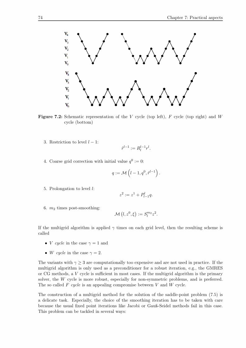
74 Chapter 7: Practical aspects
Figure 7.2: Schematic representation of the V cycle (top left), F cycle (top right) and Wcycle (bottom)
3. Restriction to level l − 1:
rl−1 := Rl−1l rl.
4. Coarse grid correction with initial value q0 := 0:
q := M(
l − 1, q0, rl−1)
.
5. Prolongation to level l:
z2 := z1 + P ll−1q.
6. m2 times post-smoothing:
M(l, z0, ξ
):= Sm2
l z2.
If the multigrid algorithm is applied γ times on each grid level, then the resulting scheme iscalled
• V cycle in the case γ = 1 and
• W cycle in the case γ = 2.
The variants with γ ≥ 3 are computationally too expensive and are not used in practice. If themultigrid algorithm is only used as a preconditioner for a robust iteration, e.g., the GMRESor CG methods, a V cycle is sufficient in most cases. If the multigrid algorithm is the primarysolver, the W cycle is more robust, especially for non-symmetric problems, and is preferred.The so called F cycle is an appealing compromise between V and W cycle.
The construction of a multigrid method for the solution of the saddle-point problem (7.5) isa delicate task. Especially, the choice of the smoothing iteration has to be taken with carebecause the usual fixed point iterations like Jacobi or Gauß-Seidel methods fail in this case.This problem can be tackled in several ways:

7.3. Solution of the instationary Navier-Stokes equations 75
1. Damped Jacobi smoother: In the case C 6= 0 the matrix A(v) is only weakly-definitewhich enables the application of standard methods like damped Jacobi iterations. Butthe resulting algorithms are not very robust and the choice of the iteration parametershas to be taken with care. Furthermore, for large Reynolds numbers this method becomesinefficient soon and does not converge anymore.
2. Block Gauß-Seidel smoother ("Vanka" smoother): A simple, but very successful,smoother is obtained for the matrix A(v) by cellwise blocking of the degrees of freedomof all physical variables within one global Gauß-Seidel iteration. This was originallyproposed for a finite difference approximation. We describe the realisation of this ideashortly: the degrees of freedom of velocity and pressure variables on one cell T or on agroup of cells are combined, i.e., numbered consecutively, and the corresponding element-wise system matrices are marked by the index "loc". These local degrees of freedom arenow iterated simultaneously within one Gauß-Seidel iteration:
Sloc(v)vkloc +Blocp
kloc = "known", B⊤
locvkloc = "known",
where Sloc := Aloc(v). This iteration runs over all blocks of cells. To increase therobustness of this method, the iteration is typically damped.
Remark 7.8 (Multigrid iteration as preconditioner) Let A be the system matrix of afinite element discretization of the linearized Navier-Stokes equations. The theory of multigridmethods is very well developed for scalar problems, whereas the situation for systems of equa-tions is not so clear. We know that the application of multigrid iterations as a preconditionerwithin an outer iteration (e.g., GMRES or CG) underlies weaker restrictions than the usage as astand-alone solver. Let M denote the operator of one multigrid step, then it is sufficient to havean upper bound on the condition number of the product MA(v), whereas in the stand-alonecase the eigenvalues of the iteration matrix B := I − MA(v) need to be bounded uniformlyaway from one. For these reasons, in the context of flow problems the multigrid algorithm isonly used as a preconditioner within a robust outer GMRES iteration. The multigrid operatorM is interpreted as an approximate inverse M ≈ A(v)−1. Of course it is not necessary, tocompute this matrix explicitly: it is sufficient, to evaluate matrix-vector products Mξ, i.e., toexecute the multigrid process for a given and fixed right hand side.
7.3 Solution of the instationary Navier-Stokes equations
7.3.1 Time-stepping schemes
The system of the instationary Navier-Stokes equations
∂tv − ν∆v+ (v · ∇)v +∇p = f
div v = 0
is, in the terminology of ordinary differential equations, a so called differential-algebraic systemof equation (DAE). The algebraic constraint
div v = 0
determines a linear manifold in the so called phase space H = H10 (Ω)
d, where the dynamics aretaking place.

76 Chapter 7: Practical aspects
To solve this problem numerically, we proceed according to Rothe’s method , i.e., we first dis-cretize in time and afterwards in every time-step the occuring quasi-stationary problem isdiscretized in space.
Remark 7.9 The discretization strategy, where we first discretize in space and afterwards intime, is called methods of lines.
Let
0 = t0 < t1 < . . . < tm < . . . < tM = T
discrete points in time,
km := tm − tm−1
the time-step sizes and
k := supmkm.
To determine the approximations vm, pm ≈ v(·, tm), p(·, tm), we first consider the so calledone-step θ scheme with the parameter θ ∈ [0, 1]:
θfm + (1− θ)fm−1 =1
km
vm − v
m−1− ν∆
θvm + (1− θ)vm−1
+ θ (vm · ∇)vm + (1− θ)(vm−1 · ∇
)vm−1
+∇θpm + (1− θ)pm−1
,
where fm := f(tm) and the constraint
div vm = 0
has to be fulfilled. Depending on the choice of θ, we obtain the following time-steppingschemes:
• θ = 1: implicit Euler
(1kmI +A+ A B
−B⊤ 0
)(vmpm
)
=
(Rm−1
0
)
,
where I is the identity/mass matrix, A the stiffness matrix, A the matrix resulting fromthe nonlinearity and B as defined before. If km → 0, then 1
kmI + A + A ≈ 1
kmI. The
resulting matrix( 1
kmI B
−B⊤ 0
)
is regular and well-conditioned. In the case km → ∞, then 1kmI + A+ A ≈ A + A. The
resulting matrix(A+ A B−B⊤ 0
)
is regular but the condition number of A is on the order O(h−2
)and the matrix therefore
becomes more and more ill-conditioned if h→ 0.
• θ = 0: explicit Euler
• θ = 12 : Crank-Nicolson

7.3. Solution of the instationary Navier-Stokes equations 77
One time-step ym−1 → ym = R(kq)ym−1 assumin the test equation
y′(t) = qy(t) t ≥ 0.
The solution of this test equation is clearly
y(t) = eqty(0).
The amplification factor R(kq) fulfils the following approximation:
R(kq) = ekq +O(kr+1
).
• A stability:|R(λ)| ≤ 1.
• Global stability:lim
Re(λ)→∞|R(λ)| ≤ 1−O(k).
• Strong A stability:lim
Re(λ)→∞|R(λ)| ≤ 1− δ < 1.
• Weak dissipation:|R(λ)| = 1−O (|Im(λ)|) , Re(λ) → 0.
7.3.2 Projection methods
7.3.2.1 Chorin method
This method is based on the implicit Euler scheme:
1km
vm − v
m−1− ν∆v
m + (vm · ∇)vm +∇pm = fm
div vm = 0
Based on the information of vm−1, pm−1 we consider the following equation:
1
k
vm − v
m−1− ν∆v
m + (vm · ∇) vm = fm.

79
Bibliography
[1] http://upload.wikimedia.org/wikipedia/commons/b/b1/Vehicle_crash_test_at_
the_General_Motors_Vehicle_Safety_and_crash_Worthiness_Laboratory.jpg
[2] http://upload.wikimedia.org/wikipedia/commons/9/97/The_Earth_seen_from_
Apollo_17.jpg
[3] http://www.nasa.gov/images/content/148709main_d4_testing_08.jpg
[4] http://upload.wikimedia.org/wikipedia/commons/f/fe/Airplane_vortex_edit.jpg
[5] http://upload.wikimedia.org/wikipedia/commons/2/2d/Aeroakustik-Windkanal-Messhalle.
JPG
[6] http://upload.wikimedia.org/wikipedia/commons/6/67/Windpark_Bassens.jpg
[7] Gert Böhme: Strömungsmechanik nichtnewtonscher Fluide, B. G. TeubnerStuttgart/Leipzig/Wiesbaden, 2. Auflage, 2000
[8] Franco Brezzi, Michel Fortin: Mixed and Hybrid Finite Element Methods, Springer New-York, 1991
[9] William J. Layton: Introduction to the Numerical Analysis of Incompressible Viscous Flows,SIAM, Computational Science & Engineering, 2008
[10] Rolf Rannacher: Numerische Mathematik 3 - Numerik von Problemen der Kontinu-umsmechanik, Lecture notes, Heidelberg University, 2008


81
Index
a posteriori error, 55a priori error, 55algorithm
modified Uzawa, 62steepest descent, 63Uzawa, 62
boundary layer, 65bubble function, 52
Clay prize, 44coefficient
diffusion, 67complement
Schur, 62convergence
super-, 59criterion
Fortin, 52curl, 10
DAE, 75damping strategy, 67derivative
directional, 10material, 16partial, 10total, 10
DG method, 70differential-algebraic equations, 75diffusion coefficient, 67directional derivative, 10Discontinuous Galerkin (DG), 70discretization
upwind, 66divergence, 10domain, 10dual problem, 56
elementMINI, 52
errora posteriori, 55
a priori, 55
fluidNewtonian, 28
formulation
mixed, 50Fortin criterion, 52function
bubble, 52Green’s, 56Lagrange, 47, 48
weight, 56functional
Lagrange, 47, 48
Galerkin-least squares(GLS), 69
GLS, 69gradient, 10
Green’s function, 56
hydrostatic pressure, 27
inf-sup condition
discrete, 33
Lagrange function, 47, 48Lagrange functional, 47, 48Laplace operator, 10
layerboundary, 65
least squares, 69linearization
Oseen, 71
Stokes, 71local projection stabilization (LPS), 70
material derivative, 16method
Discontinuous Galerkin (DG), 70line, 76Newton, 72
Rothe’s, 76steepest descent, 63
82 Index
method of lines, 76MINI element, 52mixed formulation, 50modified Uzawa algorithm, 62
nabla operator, 10Navier-Stokes equations
unsteady incompressible, 29Newton method, 72Newtonian fluid, 28
operatorLaplace, 10nabla, 10
Oseen linearization, 71
partial derivative, 10phase space, 75pressure
hydrostatic, 27primal problem, 56principal strain, 21prize
Clay, 44problem
dual, 56primal, 56saddle-point, 33Stokes, 33Sturm-Liouville, 65
refinement strategy, 56residual based stabilization, 68Reynolds number, 29Rothe’s method, 76
saddle-point problem, 33, 47, 48Schur complement, 62shear strain, 22shear tensor, 27shear viscosity, 29solution
strong, 43turbulent, 44weak, 43, 45
spacephase, 75
spatial variable, 10stabilization
local projection, 70residual based, 68
steepest descent, 63
Stokes linearization, 71Stokes problem, 33strain, 21
principal, 21shear, 22tensor, 21velocity, 23
strain tensor, 21strategy
damping, 67refinement, 56
Streamline-upwind Petrov-Galerkin, 70strong solution, 43Sturm-Liouville problem, 65superconvergence, 59SUPG, 70
tension, 50tensor
rate of deformation, 24shear, 27strain, 21
time variable, 10total derivative, 10turbulent solution, 44
upwind discretization, 66Uzawa algorithm, 62
modified, 62
variablespatial, 10time, 10
velocitystrain, 23
viscosityshear, 29volume, 29
volume viscosity, 29
weak solution, 43, 45weight function, 56