NUMERICAL METHODS IN HEAT CONDUCTION Skntu.ac.ir/DorsaPax/userfiles/file/Mechanical/... ·...

N U M E R I C A L M E T H O D SI N H E AT C O N D U C T I O N

So far we have mostly considered relatively simple heat conduction prob-lems involving simple geometries with simple boundary conditions be-cause only such simple problems can be solved analytically. But many

problems encountered in practice involve complicated geometries with com-plex boundary conditions or variable properties and cannot be solved ana-lytically. In such cases, sufficiently accurate approximate solutions can beobtained by computers using a numerical method.

Analytical solution methods such as those presented in Chapter 2 are basedon solving the governing differential equation together with the boundary con-ditions. They result in solution functions for the temperature at every point inthe medium. Numerical methods, on the other hand, are based on replacingthe differential equation by a set of n algebraic equations for the unknowntemperatures at n selected points in the medium, and the simultaneous solu-tion of these equations results in the temperature values at those discretepoints.

There are several ways of obtaining the numerical formulation of a heatconduction problem, such as the finite difference method, the finite elementmethod, the boundary element method, and the energy balance (or controlvolume) method. Each method has its own advantages and disadvantages, andeach is used in practice. In this chapter we will use primarily the energy bal-ance approach since it is based on the familiar energy balances on control vol-umes instead of heavy mathematical formulations, and thus it gives a betterphysical feel for the problem. Besides, it results in the same set of algebraicequations as the finite difference method. In this chapter, the numerical for-mulation and solution of heat conduction problems are demonstrated for bothsteady and transient cases in various geometries.

265

CHAPTER

5CONTENTS

5–1 Why Numerical Methods 266

5–2 Finite Difference Formulation ofDifferential Equations 269

5–3 One-DimensionalSteady Heat Conduction 272

5–4 Two-DimensionalSteady Heat Conduction 282

5–5 Transient Heat Conduction 291

Topic of Special Interest:

Controlling the Numerical Error 309

cen58933_ch05.qxd 9/4/2002 11:41 AM Page 265

5–1 WHY NUMERICAL METHODS?The ready availability of high-speed computers and easy-to-use powerful soft-ware packages has had a major impact on engineering education and practicein recent years. Engineers in the past had to rely on analytical skills to solvesignificant engineering problems, and thus they had to undergo a rigoroustraining in mathematics. Today’s engineers, on the other hand, have access toa tremendous amount of computation power under their fingertips, and theymostly need to understand the physical nature of the problem and interpret theresults. But they also need to understand how calculations are performed bythe computers to develop an awareness of the processes involved and the lim-itations, while avoiding any possible pitfalls.

In Chapter 2 we solved various heat conduction problems in various geo-metries in a systematic but highly mathematical manner by (1) deriving thegoverning differential equation by performing an energy balance on a differ-ential volume element, (2) expressing the boundary conditions in the propermathematical form, and (3) solving the differential equation and applying theboundary conditions to determine the integration constants. This resulted in asolution function for the temperature distribution in the medium, and the so-lution obtained in this manner is called the analytical solution of the problem.For example, the mathematical formulation of one-dimensional steady heatconduction in a sphere of radius r0 whose outer surface is maintained at a uni-form temperature of T1 with uniform heat generation at a rate of g·0 was ex-pressed as (Fig. 5–1)

� � 0

� 0 and T(r0) � T1 (5-1)

whose (analytical) solution is

T(r) � T1 � � r 2) (5-2)

This is certainly a very desirable form of solution since the temperature atany point within the sphere can be determined simply by substituting ther-coordinate of the point into the analytical solution function above. The ana-lytical solution of a problem is also referred to as the exact solution since itsatisfies the differential equation and the boundary conditions. This can beverified by substituting the solution function into the differential equation andthe boundary conditions. Further, the rate of heat flow at any location withinthe sphere or its surface can be determined by taking the derivative of the so-lution function T(r) and substituting it into Fourier’s law as

Q· (r) � �kA � �k(4�r 2) � (5-3)

The analysis above did not require any mathematical sophistication beyondthe level of simple integration, and you are probably wondering why anyonewould ask for something else. After all, the solutions obtained are exact and

4�g·0r 3

3��g·0r3k �dT

dr

g·06k

(r 20

dT(0)dr

g·0k

1r 2

ddr

�r 2 dTdr �

�

266HEAT TRANSFER

= 0dT(0)——–

dr

Solution:

+r2 = 0g0—k

dT—dr

d—dr

1—r2

·

( )

(r02 – r2)T(r) = T1 +

g0—6k

·

0Sphere

T(r0) = T1

r0

=Q(r) = –kA4 g0r3

———3

·· πdT—

dr

FIGURE 5–1The analytical solution of a problemrequires solving the governingdifferential equation and applyingthe boundary conditions.

cen58933_ch05.qxd 9/4/2002 11:41 AM 66

easy to use. Besides, they are instructive since they show clearly the func-tional dependence of temperature and heat transfer on the independent vari-able r. Well, there are several reasons for searching for alternative solutionmethods.

1 LimitationsAnalytical solution methods are limited to highly simplified problems in sim-ple geometries (Fig. 5–2). The geometry must be such that its entire surfacecan be described mathematically in a coordinate system by setting the vari-ables equal to constants. That is, it must fit into a coordinate system perfectlywith nothing sticking out or in. In the case of one-dimensional heat conduc-tion in a solid sphere of radius r0, for example, the entire outer surface can bedescribed by r � r0. Likewise, the surfaces of a finite solid cylinder of radiusr0 and height H can be described by r � r0 for the side surface and z � 0 andz � H for the bottom and top surfaces, respectively. Even minor complica-tions in geometry can make an analytical solution impossible. For example, aspherical object with an extrusion like a handle at some location is impossibleto handle analytically since the boundary conditions in this case cannot be ex-pressed in any familiar coordinate system.

Even in simple geometries, heat transfer problems cannot be solved analyt-ically if the thermal conditions are not sufficiently simple. For example, theconsideration of the variation of thermal conductivity with temperature, thevariation of the heat transfer coefficient over the surface, or the radiation heattransfer on the surfaces can make it impossible to obtain an analytical solu-tion. Therefore, analytical solutions are limited to problems that are simple orcan be simplified with reasonable approximations.

2 Better ModelingWe mentioned earlier that analytical solutions are exact solutions since theydo not involve any approximations. But this statement needs some clarifica-tion. Distinction should be made between an actual real-world problem andthe mathematical model that is an idealized representation of it. The solutionswe get are the solutions of mathematical models, and the degree of applica-bility of these solutions to the actual physical problems depends on the accu-racy of the model. An “approximate” solution of a realistic model of aphysical problem is usually more accurate than the “exact” solution of a crudemathematical model (Fig. 5–3).

When attempting to get an analytical solution to a physical problem, thereis always the tendency to oversimplify the problem to make the mathematicalmodel sufficiently simple to warrant an analytical solution. Therefore, it iscommon practice to ignore any effects that cause mathematical complicationssuch as nonlinearities in the differential equation or the boundary conditions.So it comes as no surprise that nonlinearities such as temperature dependenceof thermal conductivity and the radiation boundary conditions are seldom con-sidered in analytical solutions. A mathematical model intended for a numeri-cal solution is likely to represent the actual problem better. Therefore, thenumerical solution of engineering problems has now become the norm ratherthan the exception even when analytical solutions are available.

CHAPTER 5267

Longcylinder

h = constant

T� = constant

k = constant

Noradiation

Noradiation

T�, h h, T�

T�, h h, T�

FIGURE 5–2Analytical solution methods are

limited to simplified problemsin simple geometries.

Anoval-shaped

body

A sphere

Exact (analytical)solution of model,but crude solutionof actual problem

Approximate (numerical)solution of model,

but accurate solutionof actual problem

Realisticmodel

Simplifiedmodel

FIGURE 5–3The approximate numerical solution

of a real-world problem may be moreaccurate than the exact (analytical)

solution of an oversimplifiedmodel of that problem.

cen58933_ch05.qxd 9/4/2002 11:41 AM Page 267

3 FlexibilityEngineering problems often require extensive parametric studies to under-stand the influence of some variables on the solution in order to choose theright set of variables and to answer some “what-if ” questions. This is an iter-ative process that is extremely tedious and time-consuming if done by hand.Computers and numerical methods are ideally suited for such calculations,and a wide range of related problems can be solved by minor modifications inthe code or input variables. Today it is almost unthinkable to perform any sig-nificant optimization studies in engineering without the power and flexibilityof computers and numerical methods.

4 ComplicationsSome problems can be solved analytically, but the solution procedure is socomplex and the resulting solution expressions so complicated that it is notworth all that effort. With the exception of steady one-dimensional or transientlumped system problems, all heat conduction problems result in partialdifferential equations. Solving such equations usually requires mathematicalsophistication beyond that acquired at the undergraduate level, such as orthog-onality, eigenvalues, Fourier and Laplace transforms, Bessel and Legendrefunctions, and infinite series. In such cases, the evaluation of the solution,which often involves double or triple summations of infinite series at a speci-fied point, is a challenge in itself (Fig. 5–4). Therefore, even when the solu-tions are available in some handbooks, they are intimidating enough to scareprospective users away.

5 Human NatureAs human beings, we like to sit back and make wishes, and we like our wishesto come true without much effort. The invention of TV remote controls madeus feel like kings in our homes since the commands we give in our comfort-able chairs by pressing buttons are immediately carried out by the obedientTV sets. After all, what good is cable TV without a remote control. We cer-tainly would love to continue being the king in our little cubicle in the engi-neering office by solving problems at the press of a button on a computer(until they invent a remote control for the computers, of course). Well, thismight have been a fantasy yesterday, but it is a reality today. Practically allengineering offices today are equipped with high-powered computers withsophisticated software packages, with impressive presentation-style colorfuloutput in graphical and tabular form (Fig. 5–5). Besides, the results are asaccurate as the analytical results for all practical purposes. The computershave certainly changed the way engineering is practiced.

The discussions above should not lead you to believe that analytical solu-tions are unnecessary and that they should be discarded from the engineeringcurriculum. On the contrary, insight to the physical phenomena and engineer-ing wisdom is gained primarily through analysis. The “feel” that engineersdevelop during the analysis of simple but fundamental problems serves asan invaluable tool when interpreting a huge pile of results obtained from acomputer when solving a complex problem. A simple analysis by hand fora limiting case can be used to check if the results are in the proper range. Also,

268HEAT TRANSFER

z

L

T(r, z)

T�

rr0

0

Analytical solution:

T0

=n=1

�

∑T(r, z) – T�————–

T0 – T�

J0( nr)———— nJ1( nr0)

λλλ

sinh n(L – z)–—————

sinh ( nL)

λλ

where n’s are roots of J0( nr0) = 0λ λ

FIGURE 5–4Some analytical solutions are verycomplex and difficult to use.

FIGURE 5–5The ready availability of high-powered computers with sophisticatedsoftware packages has madenumerical solution the normrather than the exception.

cen58933_ch05.qxd 9/4/2002 11:41 AM Page 268

nothing can take the place of getting “ball park” results on a piece of paperduring preliminary discussions. The calculators made the basic arithmeticoperations by hand a thing of the past, but they did not eliminate the need forinstructing grade school children how to add or multiply.

In this chapter, you will learn how to formulate and solve heat transferproblems numerically using one or more approaches. In your professional life,you will probably solve the heat transfer problems you come across using aprofessional software package, and you are highly unlikely to write your ownprograms to solve such problems. (Besides, people will be highly skepticalof the results obtained using your own program instead of using a well-established commercial software package that has stood the test of time.) Theinsight you will gain in this chapter by formulating and solving some heattransfer problems will help you better understand the available software pack-ages and be an informed and responsible user.

5–2 FINITE DIFFERENCE FORMULATIONOF DIFFERENTIAL EQUATIONS

The numerical methods for solving differential equations are based on replac-ing the differential equations by algebraic equations. In the case of the popu-lar finite difference method, this is done by replacing the derivatives bydifferences. Below we will demonstrate this with both first- and second-orderderivatives. But first we give a motivational example.

Consider a man who deposits his money in the amount of A0 � $100 in asavings account at an annual interest rate of 18 percent, and let us try to de-termine the amount of money he will have after one year if interest is com-pounded continuously (or instantaneously). In the case of simple interest, themoney will earn $18 interest, and the man will have 100 � 100 � 0.18 �$118.00 in his account after one year. But in the case of compounding, theinterest earned during a compounding period will also earn interest for theremaining part of the year, and the year-end balance will be greater than $118.For example, if the money is compounded twice a year, the balance will be100 � 100 � (0.18/2) � $109 after six months, and 109 � 109 � (0.18/2) �$118.81 at the end of the year. We could also determine the balance A di-rectly from

A � A0(1 � i)n � ($100)(1 � 0.09)2 � $118.81 (5-4)

where i is the interest rate for the compounding period and n is the number ofperiods. Using the same formula, the year-end balance is determined formonthly, daily, hourly, minutely, and even secondly compounding, and the re-sults are given in Table 5–1.

Note that in the case of daily compounding, the year-end balance will be$119.72, which is $1.72 more than the simple interest case. (So it is no wonderthat the credit card companies usually charge interest compounded daily whendetermining the balance.) Also note that compounding at smaller time inter-vals, even at the end of each second, does not change the result, and we sus-pect that instantaneous compounding using “differential” time intervals dt willgive the same result. This suspicion is confirmed by obtaining the differential

�

CHAPTER 5269

TABLE 5–1

Year-end balance of a $100 accountearning interest at an annual rateof 18 percent for variouscompounding periods

Number Compounding of Year-End Period Periods, n Balance

1 year 1 $118.006 months 2 118.811 month 12 119.561 week 52 119.681 day 365 119.721 hour 8760 119.721 minute 525,600 119.721 second 31,536,000 119.72Instantaneous � 119.72

cen58933_ch05.qxd 9/4/2002 11:41 AM Page 269

equation dA/dt � iA for the balance A, whose solution is A � A0 exp(it). Sub-stitution yields

A � ($100)exp(0.18 � 1) � $119.72

which is identical to the result for daily compounding. Therefore, replacing adifferential time interval dt by a finite time interval of �t � 1 day gave thesame result, which leads us into believing that reasonably accurate results canbe obtained by replacing differential quantities by sufficiently small differ-ences. Next, we develop the finite difference formulation of heat conductionproblems by replacing the derivatives in the differential equations by differ-ences. In the following section we will do it using the energy balance method,which does not require any knowledge of differential equations.

Derivatives are the building blocks of differential equations, and thus wefirst give a brief review of derivatives. Consider a function f that depends onx, as shown in Figure 5–6. The first derivative of f(x) at a point is equivalentto the slope of a line tangent to the curve at that point and is defined as

� � (5-5)

which is the ratio of the increment �f of the function to the increment �x of theindependent variable as �x → 0. If we don’t take the indicated limit, we willhave the following approximate relation for the derivative:

� (5-6)

This approximate expression of the derivative in terms of differences is thefinite difference form of the first derivative. The equation above can also beobtained by writing the Taylor series expansion of the function f about thepoint x,

f(x � �x) � f(x) � �x � �x2 � · · · (5-7)

and neglecting all the terms in the expansion except the first two. The firstterm neglected is proportional to �x2, and thus the error involved in each stepof this approximation is also proportional to �x2. However, the commutativeerror involved after M steps in the direction of length L is proportional to �xsince M�x2 � (L/�x)�x2 � L�x. Therefore, the smaller the �x, the smallerthe error, and thus the more accurate the approximation.

Now consider steady one-dimensional heat transfer in a plane wall of thick-ness L with heat generation. The wall is subdivided into M sections of equalthickness �x � L/M in the x-direction, separated by planes passing throughM � 1 points 0, 1, 2, . . . , m � 1, m, m � 1, . . . , M called nodes or nodalpoints, as shown in Figure 5–7. The x-coordinate of any point m is simplyxm � m�x, and the temperature at that point is simply T(xm) � Tm.

The heat conduction equation involves the second derivatives of tempera-ture with respect to the space variables, such as d 2T/dx2, and the finite differ-ence formulation is based on replacing the second derivatives by appropriate

d 2f(x)

dx2

12

df(x)dx

f(x � �x) � f(x)�x

df(x)

dx

f(x � �x) � f(x)�x

lim�x → 0

�f�x

lim�x → 0

df(x)

dx

270HEAT TRANSFER

f (x)

xx + ∆x

∆x

∆ f

f (x + ∆x)

x

Tangent line

f (x)

FIGURE 5–6The derivative of a function at a pointrepresents the slope of the functionat that point.

T (x)

1 2 m–1

m–

… …

Tm + 1

TmTm – 1

xm m+1M–1

M

L

1–2

m+ 1–2

Plane wall

00

FIGURE 5–7Schematic of the nodes and the nodaltemperatures used in the developmentof the finite difference formulationof heat transfer in a plane wall.

cen58933_ch05.qxd 9/4/2002 11:41 AM Page 270

differences. But we need to start the process with first derivatives. UsingEq. 5–6, the first derivative of temperature dT/dx at the midpoints m � andm � of the sections surrounding the node m can be expressed as

� and � (5-8)

Noting that the second derivative is simply the derivative of the first deriva-tive, the second derivative of temperature at node m can be expressed as

� �

� (5-9)

which is the finite difference representation of the second derivative at a gen-eral internal node m. Note that the second derivative of temperature at a nodem is expressed in terms of the temperatures at node m and its two neighboringnodes. Then the differential equation

� � 0 (5-10)

which is the governing equation for steady one-dimensional heat transfer in aplane wall with heat generation and constant thermal conductivity, can be ex-pressed in the finite difference form as (Fig. 5–8)

� � 0, m � 1, 2, 3, . . . , M � 1 (5-11)

where g·m is the rate of heat generation per unit volume at node m. If the sur-face temperatures T0 and TM are specified, the application of this equation toeach of the M � 1 interior nodes results in M � 1 equations for the determi-nation of M � 1 unknown temperatures at the interior nodes. Solving theseequations simultaneously gives the temperature values at the nodes. If thetemperatures at the outer surfaces are not known, then we need to obtain twomore equations in a similar manner using the specified boundary conditions.Then the unknown temperatures at M � 1 nodes are determined by solvingthe resulting system of M � 1 equations in M � 1 unknowns simultaneously.

Note that the boundary conditions have no effect on the finite differenceformulation of interior nodes of the medium. This is not surprising since thecontrol volume used in the development of the formulation does not involveany part of the boundary. You may recall that the boundary conditions had noeffect on the differential equation of heat conduction in the medium either.

The finite difference formulation above can easily be extended to two- orthree-dimensional heat transfer problems by replacing each second derivativeby a difference equation in that direction. For example, the finite differenceformulation for steady two-dimensional heat conduction in a region with

g·mk

Tm�1 � 2Tm � Tm�1

�x2

g·

kd 2Tdx 2

Tm�1 � 2Tm � Tm�1

�x2

Tm�1 � Tm

�x�

Tm � Tm�1

�x�x

dTdx �m�

1

2

�dTdx �m�

1

2

�xd 2Tdx2 �

m

Tm�1 � Tm

�xdTdx �

m�1

2

Tm � Tm�1

�xdTdx �

m�1

2

12

12

CHAPTER 5271

∆x

Plane wall

Differential equation:

Valid at every point

+ = 0g—k

d2T—–dx2

·

Finite difference equation:

Valid at discrete points

+ = 0gm—k

Tm – 1 – 2Tm + Tm + 1—–———————∆x2

·

FIGURE 5–8The differential equation is valid at

every point of a medium, whereas thefinite difference equation is valid at

discrete points (the nodes) only.

cen58933_ch05.qxd 9/4/2002 11:41 AM Page 271

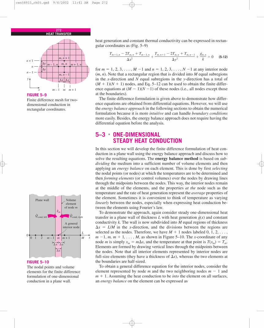
heat generation and constant thermal conductivity can be expressed in rectan-gular coordinates as (Fig. 5–9)

� � � 0 (5-12)

for m � 1, 2, 3, . . . , M �1 and n � 1, 2, 3, . . . , N �1 at any interior node(m, n). Note that a rectangular region that is divided into M equal subregionsin the x-direction and N equal subregions in the y-direction has a total of(M � 1)(N � 1) nodes, and Eq. 5–12 can be used to obtain the finite differ-ence equations at (M � 1)(N �1) of these nodes (i.e., all nodes except thoseat the boundaries).

The finite difference formulation is given above to demonstrate how differ-ence equations are obtained from differential equations. However, we will usethe energy balance approach in the following sections to obtain the numericalformulation because it is more intuitive and can handle boundary conditionsmore easily. Besides, the energy balance approach does not require having thedifferential equation before the analysis.

5–3 ONE-DIMENSIONALSTEADY HEAT CONDUCTION

In this section we will develop the finite difference formulation of heat con-duction in a plane wall using the energy balance approach and discuss how tosolve the resulting equations. The energy balance method is based on sub-dividing the medium into a sufficient number of volume elements and thenapplying an energy balance on each element. This is done by first selectingthe nodal points (or nodes) at which the temperatures are to be determined andthen forming elements (or control volumes) over the nodes by drawing linesthrough the midpoints between the nodes. This way, the interior nodes remainat the middle of the elements, and the properties at the node such as thetemperature and the rate of heat generation represent the average properties ofthe element. Sometimes it is convenient to think of temperature as varyinglinearly between the nodes, especially when expressing heat conduction be-tween the elements using Fourier’s law.

To demonstrate the approach, again consider steady one-dimensional heattransfer in a plane wall of thickness L with heat generation g·(x) and constantconductivity k. The wall is now subdivided into M equal regions of thickness�x � L/M in the x-direction, and the divisions between the regions areselected as the nodes. Therefore, we have M � 1 nodes labeled 0, 1, 2, . . . ,m �1, m, m � 1, . . . , M, as shown in Figure 5–10. The x-coordinate of anynode m is simply xm � m�x, and the temperature at that point is T(xm) � Tm.Elements are formed by drawing vertical lines through the midpoints betweenthe nodes. Note that all interior elements represented by interior nodes arefull-size elements (they have a thickness of �x), whereas the two elements atthe boundaries are half-sized.

To obtain a general difference equation for the interior nodes, consider theelement represented by node m and the two neighboring nodes m � 1 andm � 1. Assuming the heat conduction to be into the element on all surfaces,an energy balance on the element can be expressed as

�

g·m, n

k

Tm, n�1 � 2Tm, n � Tm, n�1

�y2

Tm�1, n � 2Tm, n � Tm�1, n

�x2

272HEAT TRANSFER

y

x

n + 1

m – 1 m m + 1

n

n – 1∆y

∆y

m, n + 1

m, n m + 1, nm – 1, n

m, n – 1

∆x∆x

FIGURE 5–9Finite difference mesh for two-dimensional conduction inrectangular coordinates.

A generalinterior node

Volumeelement

of node m

1 2 m – 1 xm m + 1 M

∆x

∆x∆x

L

Plane wall

gm·

Qcond, left·

Qcond, right·

00

FIGURE 5–10The nodal points and volumeelements for the finite differenceformulation of one-dimensionalconduction in a plane wall.

cen58933_ch05.qxd 9/4/2002 11:41 AM Page 272

� � �

or

Q·

cond, left � Q·

cond, right � G·element � � 0 (5-13)

since the energy content of a medium (or any part of it) does not change understeady conditions and thus �Eelement � 0. The rate of heat generation withinthe element can be expressed as

G·element � g·mVelement � g·m A�x (5-14)

where g·m is the rate of heat generation per unit volume in W/m3 evaluated atnode m and treated as a constant for the entire element, and A is heat transferarea, which is simply the inner (or outer) surface area of the wall.

Recall that when temperature varies linearly, the steady rate of heat con-duction across a plane wall of thickness L can be expressed as

Q·

cond � kA (5-15)

where �T is the temperature change across the wall and the direction of heattransfer is from the high temperature side to the low temperature. In the caseof a plane wall with heat generation, the variation of temperature is not linearand thus the relation above is not applicable. However, the variation of tem-perature between the nodes can be approximated as being linear in the deter-mination of heat conduction across a thin layer of thickness �x between twonodes (Fig. 5–11). Obviously the smaller the distance �x between two nodes,the more accurate is this approximation. (In fact, such approximations are thereason for classifying the numerical methods as approximate solution meth-ods. In the limiting case of �x approaching zero, the formulation becomes ex-act and we obtain a differential equation.) Noting that the direction of heattransfer on both surfaces of the element is assumed to be toward the node m,the rate of heat conduction at the left and right surfaces can be expressed as

Q·

cond, left � kA and Q·

cond, right � kA (5-16)

Substituting Eqs. 5–14 and 5–16 into Eq. 5–13 gives

kA � kA � g·m A�x � 0 (5-17)

which simplifies to

� � 0, m � 1, 2, 3, . . . , M � 1 (5-18)g·mk

Tm�1 � 2Tm � Tm�1

�x2

Tm�1 � Tm

�x

Tm�1 � Tm

�x

Tm�1 � Tm

�x

Tm�1 � Tm

�x

�TL

�Eelement

�t

�Rate of changeof the energy

content ofthe element ��

Rate of heatgenerationinside theelement ��

Rate of heatconductionat the right

surface ��Rate of heatconductionat the leftsurface �

CHAPTER 5273

kATm + 1 – Tm————–

∆xkA

Tm – 1 – Tm————–∆x

∆x

m – 1 m

k

Volumeelement

Linear

Linear

AA

m + 1

∆x

Tm

Tm + 1

Tm – 1

FIGURE 5–11In finite difference formulation, the

temperature is assumed to varylinearly between the nodes.

cen58933_ch05.qxd 9/4/2002 11:41 AM Page 273

which is identical to the difference equation (Eq. 5–11) obtained earlier.Again, this equation is applicable to each of the M � 1 interior nodes, and itsapplication gives M � 1 equations for the determination of temperatures atM � 1 nodes. The two additional equations needed to solve for the M � 1 un-known nodal temperatures are obtained by applying the energy balance on thetwo elements at the boundaries (unless, of course, the boundary temperaturesare specified).

You are probably thinking that if heat is conducted into the element fromboth sides, as assumed in the formulation, the temperature of the medium willhave to rise and thus heat conduction cannot be steady. Perhaps a more realis-tic approach would be to assume the heat conduction to be into the element onthe left side and out of the element on the right side. If you repeat the formu-lation using this assumption, you will again obtain the same result since theheat conduction term on the right side in this case will involve Tm � Tm � 1 in-stead of Tm � 1 � Tm, which is subtracted instead of being added. Therefore,the assumed direction of heat conduction at the surfaces of the volume ele-ments has no effect on the formulation, as shown in Figure 5–12. (Besides, theactual direction of heat transfer is usually not known.) However, it is conve-nient to assume heat conduction to be into the element at all surfaces and notworry about the sign of the conduction terms. Then all temperature differencesin conduction relations are expressed as the temperature of the neighboringnode minus the temperature of the node under consideration, and all conduc-tion terms are added.

Boundary ConditionsAbove we have developed a general relation for obtaining the finite differenceequation for each interior node of a plane wall. This relation is not applicableto the nodes on the boundaries, however, since it requires the presence ofnodes on both sides of the node under consideration, and a boundary nodedoes not have a neighboring node on at least one side. Therefore, we need toobtain the finite difference equations of boundary nodes separately. This isbest done by applying an energy balance on the volume elements of boundarynodes.

Boundary conditions most commonly encountered in practice are the spec-ified temperature, specified heat flux, convection, and radiation boundaryconditions, and here we develop the finite difference formulations for themfor the case of steady one-dimensional heat conduction in a plane wall ofthickness L as an example. The node number at the left surface at x � 0 is 0,and at the right surface at x � L it is M. Note that the width of the volume el-ement for either boundary node is �x/2.

The specified temperature boundary condition is the simplest boundarycondition to deal with. For one-dimensional heat transfer through a plane wallof thickness L, the specified temperature boundary conditions on both the leftand right surfaces can be expressed as (Fig. 5–13)

T(0) � T0 � Specified value

T(L) � TM � Specified value (5-19)

where T0 and Tm are the specified temperatures at surfaces at x � 0 and x � L,respectively. Therefore, the specified temperature boundary conditions are

274HEAT TRANSFER

kAT1 – T2———

∆xkA

T2 – T3———∆x

1 2

Volumeelement

of node 2

3

g2A∆x·

kA

or

(a) Assuming heat transfer to be out of thevolume element at the right surface.

T1 – T2———∆x

– kAT2 – T3———

∆x+ g2A∆x = 0·

T1 – 2T2 + T3 + g2A∆x2 / k = 0·

kAT1 – T2———

∆xkA

T3 – T2———∆x

1 2

Volumeelement

of node 2

3

g2A∆x·

kA

or

(b) Assuming heat transfer to be into thevolume element at all surfaces.

T1 – T2———∆x

+ kAT3 – T2———

∆x+ g2A∆x = 0·

T1 – 2T2 + T3 + g2A∆x2 / k = 0·

FIGURE 5–12The assumed direction of heat transferat surfaces of a volume element hasno effect on the finite differenceformulation.

cen58933_ch05.qxd 9/4/2002 11:41 AM Page 274

incorporated by simply assigning the given surface temperatures to the bound-ary nodes. We do not need to write an energy balance in this case unless wedecide to determine the rate of heat transfer into or out of the medium after thetemperatures at the interior nodes are determined.

When other boundary conditions such as the specified heat flux, convection,radiation, or combined convection and radiation conditions are specified at aboundary, the finite difference equation for the node at that boundary is ob-tained by writing an energy balance on the volume element at that boundary.The energy balance is again expressed as

Q·

� G·element � 0 (5-20)

for heat transfer under steady conditions. Again we assume all heat transfer tobe into the volume element from all surfaces for convenience in formulation,except for specified heat flux since its direction is already specified. Specifiedheat flux is taken to be a positive quantity if into the medium and a negativequantity if out of the medium. Then the finite difference formulation at thenode m � 0 (at the left boundary where x � 0) of a plane wall of thickness Lduring steady one-dimensional heat conduction can be expressed as (Fig.5–14)

Q·

left surface � kA � g·0(A�x/2) � 0 (5-21)

where A�x/2 is the volume of the volume element (note that the boundary ele-ment has half thickness), g·0 is the rate of heat generation per unit volume (inW/m3) at x � 0, and A is the heat transfer area, which is constant for a planewall. Note that we have �x in the denominator of the second term instead of�x/2. This is because the ratio in that term involves the temperature differencebetween nodes 0 and 1, and thus we must use the distance between those twonodes, which is �x.

The finite difference form of various boundary conditions can be obtainedfrom Eq. 5–21 by replacing Q

·left surface by a suitable expression. Next this is

done for various boundary conditions at the left boundary.

1. Specified Heat Flux Boundary Condition

q·0A � kA � g·0(A�x/2) � 0 (5-22)

Special case: Insulated Boundary (q·0 � 0)

kA � g·0(A�x/2) � 0 (5-23)

2. Convection Boundary Condition

hA(T� � T0) � kA � g·0(A�x/2) � 0 (5-24)T1 � T0

�x

T1 � T0

�x

T1 � T0

�x

T1 � T0

�x

�all sides

CHAPTER 5275

100

2

T0 = 35°C

TM = 82°C

M

L

Plane wall

82°C35°C

…

FIGURE 5–13Finite difference formulation ofspecified temperature boundary

conditions on both surfacesof a plane wall.

100

2 xL

Volume elementof node 0

…∆x ∆x

kAT1 – T0———

∆xQleft surface·

∆x—–2

g0·

Qleft surface + kAT1 – T0———

∆x∆x—–2

+ g0A· = 0·

FIGURE 5–14Schematic for the finite difference

formulation of the left boundarynode of a plane wall.

cen58933_ch05.qxd 9/4/2002 11:41 AM Page 275

3. Radiation Boundary Condition

A( ) � kA � g·0(A�x/2) � 0 (5-25)

4. Combined Convection and Radiation Boundary Condition(Fig. 5–15)

hA(T� � T0) � A( ) � kA � g·0(A�x/2) � 0 (5-26)

or

hcombined A(T� � T0) � kA � g·0(A�x/2) � 0 (5-27)

5. Combined Convection, Radiation, and Heat Flux BoundaryCondition

q·0A � hA(T� � T0) � A( ) � kA � g·0(A�x/2) � 0 (5-28)

6. Interface Boundary Condition Two different solid media A and Bare assumed to be in perfect contact, and thus at the same temperatureat the interface at node m (Fig. 5–16). Subscripts A and B indicateproperties of media A and B, respectively.

kAA � kBA � g·A, m(A�x/2) � g·B, m(A�x/2) � 0 (5-29)

In these relations, q·0 is the specified heat flux in W/m2, h is the convectioncoefficient, hcombined is the combined convection and radiation coefficient, T� isthe temperature of the surrounding medium, Tsurr is the temperature of thesurrounding surfaces, is the emissivity of the surface, and is the Stefan–Boltzman constant. The relations above can also be used for node M on theright boundary by replacing the subscript “0” by “M” and the subscript “1” by“M � 1”.

Note that absolute temperatures must be used in radiation heat transfercalculations, and all temperatures should be expressed in K or R when aboundary condition involves radiation to avoid mistakes. We usually try toavoid the radiation boundary condition even in numerical solutions since itcauses the finite difference equations to be nonlinear, which are more difficultto solve.

Treating Insulated Boundary Nodes as Interior Nodes:The Mirror Image ConceptOne way of obtaining the finite difference formulation of a node on an insu-lated boundary is to treat insulation as “zero” heat flux and to write an energybalance, as done in Eq. 5–23. Another and more practical way is to treat thenode on an insulated boundary as an interior node. Conceptually this is done

Tm�1 � Tm

�x

Tm�1 � Tm

�x

T1 � T0

�xT 4

surr � T 40

T1 � T0

�x

T1 � T0

�xT 4

surr � T 40

T1 � T0

�xT 4

surr � T 40

276HEAT TRANSFER

100

hA(T� – T0)

2 x

L

A

…∆x ∆x

kAT1 – T0———

∆x

∆x—–2

g0·

Tsurr

ε

A(T4surr – T4

0)εσ

hA(T� – T0) + A(T4surr – T4

0)εσ

T1 – T0———∆x

∆x—–2

+ g0A· = 0 + kA

FIGURE 5–15Schematic for the finite differenceformulation of combined convectionand radiation on the left boundaryof a plane wall.

mm – 1 m + 1 x

A A

∆x ∆x

kB ATm + 1 – Tm————–

∆xkAA

Tm – 1 – Tm————–∆x

∆x—–2

∆x—–2

gB,m·gA,m

·

Interface

Medium AkA

Medium BkB

Tm – 1 – Tm————–∆x

∆x—–2

+ gB,mA· = 0∆x—–2

+ gA,mA·

kAATm + 1 – Tm————–

∆x + kB A

FIGURE 5–16Schematic for the finite differenceformulation of the interface boundarycondition for two mediums A and Bthat are in perfect thermal contact.

cen58933_ch05.qxd 9/4/2002 11:41 AM Page 276

by replacing the insulation on the boundary by a mirror and considering thereflection of the medium as its extension (Fig. 5–17). This way the node nextto the boundary node appears on both sides of the boundary node because ofsymmetry, converting it into an interior node. Then using the general formula(Eq. 5–18) for an interior node, which involves the sum of the temperatures ofthe adjoining nodes minus twice the node temperature, the finite differenceformulation of a node m � 0 on an insulated boundary of a plane wall can beexpressed as

� � 0 → � � 0 (5-30)

which is equivalent to Eq. 5–23 obtained by the energy balance approach.The mirror image approach can also be used for problems that possess ther-

mal symmetry by replacing the plane of symmetry by a mirror. Alternately, wecan replace the plane of symmetry by insulation and consider only half of themedium in the solution. The solution in the other half of the medium is sim-ply the mirror image of the solution obtained.

g·0k

T1 � 2T0 � T1

�x2

g·mk

Tm�1 � 2Tm � Tm�1

�x2

CHAPTER 5277

x0 1

Insulatedboundary

node

2

xx 0 1

Equivalentinteriornode

Mirror

Mirrorimage

212

Insulation

FIGURE 5–17A node on an insulated boundary

can be treated as an interior node byreplacing the insulation by a mirror.

EXAMPLE 5–1 Steady Heat Conduction in a Large Uranium Plate

Consider a large uranium plate of thickness L � 4 cm and thermal conductivityk � 28 W/m · °C in which heat is generated uniformly at a constant rate ofg· � 5 � 106 W/m3. One side of the plate is maintained at 0°C by iced waterwhile the other side is subjected to convection to an environment at T� � 30°Cwith a heat transfer coefficient of h � 45 W/m2 · °C, as shown in Figure 5–18.Considering a total of three equally spaced nodes in the medium, two at theboundaries and one at the middle, estimate the exposed surface temperature ofthe plate under steady conditions using the finite difference approach.

SOLUTION A uranium plate is subjected to specified temperature on one sideand convection on the other. The unknown surface temperature of the plate isto be determined numerically using three equally spaced nodes.Assumptions 1 Heat transfer through the wall is steady since there is no in-dication of any change with time. 2 Heat transfer is one-dimensional sincethe plate is large relative to its thickness. 3 Thermal conductivity is constant. 4 Radiation heat transfer is negligible.Properties The thermal conductivity is given to be k � 28 W/m · °C.Analysis The number of nodes is specified to be M � 3, and they are chosento be at the two surfaces of the plate and the midpoint, as shown in the figure.Then the nodal spacing �x becomes

�x � � � 0.02 m

We number the nodes 0, 1, and 2. The temperature at node 0 is given to beT0 � 0°C, and the temperatures at nodes 1 and 2 are to be determined. Thisproblem involves only two unknown nodal temperatures, and thus we need tohave only two equations to determine them uniquely. These equations are ob-tained by applying the finite difference method to nodes 1 and 2.

0.04 m3 � 1

LM � 1

00

1 2 xL

Uraniumplate

k = 28 W/m·°C

g = 5 × 106 W/m3

h

T�

0°C

·

FIGURE 5–18Schematic for Example 5–1.

cen58933_ch05.qxd 9/4/2002 11:41 AM Page 277

278HEAT TRANSFER

Node 1 is an interior node, and the finite difference formulation at that nodeis obtained directly from Eq. 5–18 by setting m � 1:

� � 0 → � � 0 → 2T1 � T2 �

(1)

Node 2 is a boundary node subjected to convection, and the finite differenceformulation at that node is obtained by writing an energy balance on the volumeelement of thickness �x/2 at that boundary by assuming heat transfer to be intothe medium at all sides:

hA(T� � T2) � kA � g·2(A�x/2) � 0

Canceling the heat transfer area A and rearranging give

T1 � T2 � � T� � (2)

Equations (1) and (2) form a system of two equations in two unknowns T1 andT2. Substituting the given quantities and simplifying gives

2T1 � T2 � 71.43 (in °C)

T1 � 1.032T2 � �36.68 (in °C)

This is a system of two algebraic equations in two unknowns and can be solvedeasily by the elimination method. Solving the first equation for T1 and substi-tuting into the second equation result in an equation in T2 whose solution is

T2 � 136.1°C

This is the temperature of the surface exposed to convection, which is thedesired result. Substitution of this result into the first equation gives T1 �103.8°C, which is the temperature at the middle of the plate.

Discussion The purpose of this example is to demonstrate the use of the finitedifference method with minimal calculations, and the accuracy of the resultwas not a major concern. But you might still be wondering how accurate the re-sult obtained above is. After all, we used a mesh of only three nodes for theentire plate, which seems to be rather crude. This problem can be solved ana-lytically as described in Chapter 2, and the analytical (exact) solution can beshown to be

T(x) � x �

Substituting the given quantities, the temperature of the exposed surface of theplate at x � L � 0.04 m is determined to be 136.0°C, which is almost identi-cal to the result obtained here with the approximate finite difference method(Fig. 5–19). Therefore, highly accurate results can be obtained with numericalmethods by using a limited number of nodes.

g·x2

2k0.5g·hL2/k � g·L � T�h

hL � k

g·2�x2

2kh�x

k�1 �h�x

k �

T1 � T2

�x

g·1�x2

kg·1k

0 � 2T1 � T2

�x2

g·1k

T0 � 2T1 � T2

�x2

h

T�

0 1 2 x

Plate

2 cm

Finite difference solution:

T2 = 136.1°C

Exact solution:

T2 = 136.0°C

2 cm

FIGURE 5–19Despite being approximate in nature,highly accurate results can beobtained by numerical methods.

cen58933_ch05.qxd 9/4/2002 11:41 AM Page 278

CHAPTER 5279

EXAMPLE 5–2 Heat Transfer from Triangular Fins

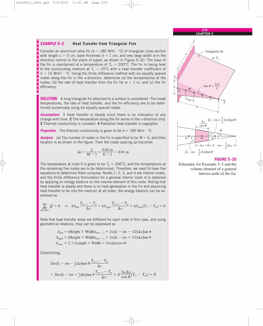
Consider an aluminum alloy fin (k � 180 W/m · °C) of triangular cross sectionwith length L � 5 cm, base thickness b � 1 cm, and very large width w in thedirection normal to the plane of paper, as shown in Figure 5–20. The base ofthe fin is maintained at a temperature of T0 � 200°C. The fin is losing heatto the surrounding medium at T� � 25°C with a heat transfer coefficient ofh � 15 W/m2 · °C. Using the finite difference method with six equally spacednodes along the fin in the x-direction, determine (a) the temperatures at thenodes, (b) the rate of heat transfer from the fin for w � 1 m, and (c) the finefficiency.

SOLUTION A long triangular fin attached to a surface is considered. The nodaltemperatures, the rate of heat transfer, and the fin efficiency are to be deter-mined numerically using six equally spaced nodes.

Assumptions 1 Heat transfer is steady since there is no indication of anychange with time. 2 The temperature along the fin varies in the x direction only.3 Thermal conductivity is constant. 4 Radiation heat transfer is negligible.

Properties The thermal conductivity is given to be k � 180 W/m · °C.

Analysis (a) The number of nodes in the fin is specified to be M � 6, and theirlocation is as shown in the figure. Then the nodal spacing �x becomes

�x � � � 0.01 m

The temperature at node 0 is given to be T0 � 200°C, and the temperatures atthe remaining five nodes are to be determined. Therefore, we need to have fiveequations to determine them uniquely. Nodes 1, 2, 3, and 4 are interior nodes,and the finite difference formulation for a general interior node m is obtainedby applying an energy balance on the volume element of this node. Noting thatheat transfer is steady and there is no heat generation in the fin and assumingheat transfer to be into the medium at all sides, the energy balance can be ex-pressed as

Q·

� 0 → kAleft � kAright � hAconv(T� � Tm) � 0

Note that heat transfer areas are different for each node in this case, and usinggeometrical relations, they can be expressed as

Aleft � (Height � Width)@m � � 2w[L � (m � 1/2)�x]tan �

Aright � (Height � Width)@m � � 2w[L � (m � 1/2)�x]tan �

Aconv � 2 � Length � Width � 2w(�x/cos �)

Substituting,

2kw[L � (m � )�x]tan �

� 2kw[L � (m � )�x]tan � � h (T� � Tm) � 02w�xcos �

Tm�1 � Tm

�x12

Tm�1 � Tm

�x12

12

12

Tm�1 � Tm

�x

Tm�1 � Tm

�x�all sides

0.05 m6 � 1

LM � 1

∆x

θ

θ

m – 1 m m + 1

L – (m – )∆x1–2

θ∆x——–

cos

[L – (m + )∆x]tan1–2

θ

[L – (m – )∆x]tan1–2

θ

12

34

5

0

∆x

L

wh, T�

T0

x

b

Triangular fin

tan =θ b/2—–L

FIGURE 5–20Schematic for Example 5–2 and the

volume element of a generalinterior node of the fin.

cen58933_ch05.qxd 9/4/2002 11:41 AM Page 279

280HEAT TRANSFER

Dividing each term by 2kwL tan �/�x gives

(Tm � 1 � Tm) � (Tm � 1 � Tm)

� (T� � Tm) � 0

Note that

tan � � � 0.1 → � � tan�10.1 � 5.71°

Also, sin 5.71° � 0.0995. Then the substitution of known quantities gives

(5.5 � m)Tm � 1 � (10.00838 � 2m)Tm � (4.5 � m)Tm � 1 � �0.209

Now substituting 1, 2, 3, and 4 for m results in these finite difference equa-tions for the interior nodes:

m � 1: �8.00838T1 � 3.5T2 � �900.209 (1)

m � 2: 3.5T1 � 6.00838T2 � 2.5T3 � �0.209 (2)

m � 3: 2.5T2 � 4.00838T3 � 1.5T4 � �0.209 (3)

m � 4: 1.5T3 � 2.00838T4 � 0.5T5 � �0.209 (4)

The finite difference equation for the boundary node 5 is obtained by writing anenergy balance on the volume element of length �x/2 at that boundary, again byassuming heat transfer to be into the medium at all sides (Fig. 5–21):

kAleft � hAconv (T� � T5) � 0

where

Aleft � 2w tan � and Aconv � 2w

Canceling w in all terms and substituting the known quantities gives

T4 � 1.00838T5 � �0.209 (5)

Equations (1) through (5) form a linear system of five algebraic equations in fiveunknowns. Solving them simultaneously using an equation solver gives

T1 � 198.6°C, T2 � 197.1°C, T3 � 195.7°C,

T4 � 194.3°C, T5 � 192.9°C

which is the desired solution for the nodal temperatures.

(b) The total rate of heat transfer from the fin is simply the sum of the heattransfer from each volume element to the ambient, and for w � 1 m it is deter-mined from

�x/2cos �

�x2

T4 � T5

�x

b/2L

�0.5 cm5 cm

h(�x)2

kL sin �

�1 � (m � 12)

�xL ��1 � (m � 1

2)

�xL �

4 5θ

∆x—–2

∆x—–2

tan θ∆x—–2

∆x /2—–—cos θ

FIGURE 5–21Schematic of the volume element ofnode 5 at the tip of a triangular fin.

cen58933_ch05.qxd 9/4/2002 11:41 AM Page 280

The finite difference formulation of steady heat conduction problems usu-ally results in a system of N algebraic equations in N unknown nodal temper-atures that need to be solved simultaneously. When N is small (such as 2 or 3),we can use the elementary elimination method to eliminate all unknowns ex-cept one and then solve for that unknown (see Example 5–1). The other un-knowns are then determined by back substitution. When N is large, which isusually the case, the elimination method is not practical and we need to use amore systematic approach that can be adapted to computers.

There are numerous systematic approaches available in the literature, andthey are broadly classified as direct and iterative methods. The direct meth-ods are based on a fixed number of well-defined steps that result in the solu-tion in a systematic manner. The iterative methods, on the other hand, arebased on an initial guess for the solution that is refined by iteration until aspecified convergence criterion is satisfied (Fig. 5–22). The direct methodsusually require a large amount of computer memory and computation time,

CHAPTER 5281

Q·

fin � Q·

element, m � hAconv, m(Tm � T�)

Noting that the heat transfer surface area is w�x/cos � for the boundary nodes0 and 5, and twice as large for the interior nodes 1, 2, 3, and 4, we have

Q·

fin � h [(T0 � T�) � 2(T1 � T�) � 2(T2 � T�) � 2(T3 � T�)

� 2(T4 � T�) � (T5 � T�)]

� h [T0 � 2(T1 � T2 � T3 � T4) � T5 � 10T�]

� (15 W/m2 · °C) [200 � 2 � 785.7 � 192.9 � 10 � 25]

� 258.4 W

(c) If the entire fin were at the base temperature of T0 � 200°C, the total rateof heat transfer from the fin for w � 1 m would be

Q·

max � hAfin, total (T0 � T�) � h(2wL/cos �)(T0 � T�)

� (15 W/m2 · °C)[2(1 m)(0.05 m)/cos5.71°](200 � 25)°C

� 263.8 W

Then the fin efficiency is determined from

�fin � � � 0.98

which is less than 1, as expected. We could also determine the fin efficiency inthis case from the proper fin efficiency curve in Chapter 3, which is based onthe analytical solution. We would read 0.98 for the fin efficiency, which is iden-tical to the value determined above numerically.

258.4 W263.8 W

Q·fin

Q·max

(1 m)(0.01 m)cos 5.71°

w�xcos �

w�xcos �

�5

m�0�

5

m�0

Direct methods:Solve in a systematic manner following aseries of well-defined steps.

Iterative methods:Start with an initial guess for the solution,and iterate until solution converges.

FIGURE 5–22Two general categories of solution

methods for solving systemsof algebraic equations.

cen58933_ch05.qxd 9/4/2002 11:41 AM Page 281

and they are more suitable for systems with a relatively small number of equa-tions. The computer memory requirements for iterative methods are minimal,and thus they are usually preferred for large systems. The convergence of it-erative methods to the desired solution, however, may pose a problem.

5–4 TWO-DIMENSIONALSTEADY HEAT CONDUCTION

In Section 5–3 we considered one-dimensional heat conduction and assumedheat conduction in other directions to be negligible. Many heat transfer prob-lems encountered in practice can be approximated as being one-dimensional,but this is not always the case. Sometimes we need to consider heat transfer inother directions as well when the variation of temperature in other directionsis significant. In this section we will consider the numerical formulation andsolution of two-dimensional steady heat conduction in rectangular coordinatesusing the finite difference method. The approach presented below can be ex-tended to three-dimensional cases.

Consider a rectangular region in which heat conduction is significant in thex- and y-directions. Now divide the x-y plane of the region into a rectangularmesh of nodal points spaced �x and �y apart in the x- and y-directions,respectively, as shown in Figure 5–23, and consider a unit depth of �z � 1in the z-direction. Our goal is to determine the temperatures at the nodes,and it is convenient to number the nodes and describe their position bythe numbers instead of actual coordinates. A logical numbering scheme fortwo-dimensional problems is the double subscript notation (m, n) wherem � 0, 1, 2, . . . , M is the node count in the x-direction and n � 0, 1, 2, . . . , Nis the node count in the y-direction. The coordinates of the node (m, n) aresimply x � m�x and y � n�y, and the temperature at the node (m, n) isdenoted by Tm, n.

Now consider a volume element of size �x � �y � 1 centered about a gen-eral interior node (m, n) in a region in which heat is generated at a rate of g· andthe thermal conductivity k is constant, as shown in Figure 5–24. Againassuming the direction of heat conduction to be toward the node underconsideration at all surfaces, the energy balance on the volume element can beexpressed as

� �

or

Q·

cond, left � Q·

cond, top � Q·

cond, right � Q·

cond, bottom� G·element � � 0 (5-31)

for the steady case. Again assuming the temperatures between the adja-cent nodes to vary linearly and noting that the heat transfer area isAx � �y � 1 � �y in the x-direction and Ay � �x � 1 � �x in the y-direction,the energy balance relation above becomes

�Eelement

�t

�Rate of change ofthe energy content

of the element �� Rate of heatgeneration inside

the element ��Rate of heat conductionat the left, top, right,and bottom surfaces �

�

282HEAT TRANSFER

y

x

10

2

N

n – 1n

n + 1

0 1 2m – 1

mm + 1

M…

……

…

Node (m, n)∆y∆y

∆x ∆x

FIGURE 5–23The nodal network for the finitedifference formulation of two-dimensional conduction inrectangular coordinates.

n – 1

n

n + 1

m – 1 m m + 1

∆x∆x

m, n

Volumeelement

m + 1, n

m, n + 1

m, n – 1

m – 1, ngm, n·

∆y

∆y

y

x

FIGURE 5–24The volume element of a generalinterior node (m, n) for two-dimensional conduction inrectangular coordinates.

cen58933_ch05.qxd 9/4/2002 11:41 AM Page 282

k�y � k�x � k�y

� k�x � g·m, n �x �y � 0 (5-32)

Dividing each term by �x � �y and simplifying gives

� � � 0 (5-33)

for m � 1, 2, 3, . . . , M � 1 and n � 1, 2, 3, . . . , N � 1. This equation is iden-tical to Eq. 5–12 obtained earlier by replacing the derivatives in the differen-tial equation by differences for an interior node (m, n). Again a rectangularregion M equally spaced nodes in the x-direction and N equally spaced nodesin the y-direction has a total of (M � 1)(N � 1) nodes, and Eq. 5–33 can beused to obtain the finite difference equations at all interior nodes.

In finite difference analysis, usually a square mesh is used for sim-plicity (except when the magnitudes of temperature gradients in the x- andy-directions are very different), and thus �x and �y are taken to be the same.Then �x � �y � l, and the relation above simplifies to

Tm � 1, n � Tm � 1, n � Tm, n � 1 � Tm, n � 1 � 4Tm, n � � 0 (5-34)

That is, the finite difference formulation of an interior node is obtained byadding the temperatures of the four nearest neighbors of the node, subtractingfour times the temperature of the node itself, and adding the heat generationterm. It can also be expressed in this form, which is easy to remember:

Tleft � Ttop � Tright � Tbottom � 4Tnode � � 0 (5-35)

When there is no heat generation in the medium, the finite difference equa-tion for an interior node further simplifies to Tnode � (Tleft � Ttop � Tright �Tbottom)/4, which has the interesting interpretation that the temperature of eachinterior node is the arithmetic average of the temperatures of the four neigh-boring nodes. This statement is also true for the three-dimensional problemsexcept that the interior nodes in that case will have six neighboring nodes in-stead of four.

Boundary NodesThe development of finite difference formulation of boundary nodes in two-(or three-) dimensional problems is similar to the development in the one-dimensional case discussed earlier. Again, the region is partitioned betweenthe nodes by forming volume elements around the nodes, and an energy bal-ance is written for each boundary node. Various boundary conditions can behandled as discussed for a plane wall, except that the volume elementsin the two-dimensional case involve heat transfer in the y-direction as well asthe x-direction. Insulated surfaces can still be viewed as “mirrors, ” and the

g· nodel 2

k

g·m, nl 2

k

g·m, n

k

Tm, n�1 � 2Tm, n � Tm, n�1

�y2

Tm�1, n � 2Tm, n � Tm�1, n

�x2

Tm, n�1 � Tm, n

�y

Tm�1, n � Tm, n

�x

Tm, n�1 � Tm, n

�y

Tm�1, n � Tm, n

�x

CHAPTER 5283

cen58933_ch05.qxd 9/4/2002 11:41 AM Page 283

mirror image concept can be used to treat nodes on insulated boundaries as in-terior nodes.

For heat transfer under steady conditions, the basic equation to keep in mindwhen writing an energy balance on a volume element is (Fig. 5–25)

Q·

� g·Velement � 0 (5-36)

whether the problem is one-, two-, or three-dimensional. Again we assume,for convenience in formulation, all heat transfer to be into the volume ele-ment from all surfaces except for specified heat flux, whose direction is al-ready specified. This is demonstrated in Example 5–3 for various boundaryconditions.

�all sides

284HEAT TRANSFER

∆x

∆y

1

Volume elementof node 2

2

h, T�

4

3

Boundarysubjected

to convection

Qleft·

Qbottom·

Qtop·

Qright·

Qleft + Qtop + Qright + Qbottom + · · · ·

= 0g2V2——

k

·

FIGURE 5–25The finite difference formulation ofa boundary node is obtained bywriting an energy balanceon its volume element.

EXAMPLE 5–3 Steady Two-Dimensional Heat Conductionin L-Bars

Consider steady heat transfer in an L-shaped solid body whose cross section isgiven in Figure 5–26. Heat transfer in the direction normal to the plane of thepaper is negligible, and thus heat transfer in the body is two-dimensional. Thethermal conductivity of the body is k � 15 W/m · °C, and heat is generated inthe body at a rate of g· � 2 � 106 W/m3. The left surface of the body is insu-lated, and the bottom surface is maintained at a uniform temperature of 90°C.The entire top surface is subjected to convection to ambient air at T� � 25°Cwith a convection coefficient of h � 80 W/m2 · °C, and the right surface is sub-jected to heat flux at a uniform rate of q·R � 5000 W/m2. The nodal network ofthe problem consists of 15 equally spaced nodes with �x � �y � 1.2 cm, asshown in the figure. Five of the nodes are at the bottom surface, and thus theirtemperatures are known. Obtain the finite difference equations at the remain-ing nine nodes and determine the nodal temperatures by solving them.

SOLUTION Heat transfer in a long L-shaped solid bar with specified boundaryconditions is considered. The nine unknown nodal temperatures are to be de-termined with the finite difference method.Assumptions 1 Heat transfer is steady and two-dimensional, as stated. 2 Ther-mal conductivity is constant. 3 Heat generation is uniform. 4 Radiation heattransfer is negligible.Properties The thermal conductivity is given to be k � 15 W/m · °C.Analysis We observe that all nodes are boundary nodes except node 5, whichis an interior node. Therefore, we will have to rely on energy balances to obtainthe finite difference equations. But first we form the volume elements by parti-tioning the region among the nodes equitably by drawing dashed lines betweenthe nodes. If we consider the volume element represented by an interior nodeto be full size (i.e., �x � �y � 1), then the element represented by a regularboundary node such as node 2 becomes half size (i.e., �x � �y/2 � 1), anda corner node such as node 1 is quarter size (i.e., �x/2 � �y/2 � 1). KeepingEq. 5–36 in mind for the energy balance, the finite difference equations foreach of the nine nodes are obtained as follows:

(a) Node 1. The volume element of this corner node is insulated on the left andsubjected to convection at the top and to conduction at the right and bottomsurfaces. An energy balance on this element gives [Fig. 5–27a]

12 13 14 151110

6 7 8 954

321

x

y

∆x ∆x ∆x ∆x ∆x

∆y

∆y

90°C

qR·

∆x = ∆y = l

Convectionh, T�

FIGURE 5–26Schematic for Example 5–3 andthe nodal network (the boundariesof volume elements of the nodes areindicated by dashed lines).

h, T�

1

4

2

(a) Node 1

h, T�

21

5

3

(b) Node 2

FIGURE 5–27Schematics for energy balances on thevolume elements of nodes 1 and 2.

cen58933_ch05.qxd 9/4/2002 11:41 AM Page 284

CHAPTER 5285

0 � h (T� � T1) � k � k � g·1 � 0

Taking �x � �y � l, it simplifies to

– T1 � T2 � T4 � � T� �

(b) Node 2. The volume element of this boundary node is subjected to con-vection at the top and to conduction at the right, bottom, and left surfaces. Anenergy balance on this element gives [Fig. 5–27b]

h�x(T� � T2) � k � k�x � k � g·2�x � 0


T1 � T2 � T3 � 2T5 � � T� �

(c) Node 3. The volume element of this corner node is subjected to convectionat the top and right surfaces and to conduction at the bottom and left surfaces.An energy balance on this element gives [Fig. 5–28a]

h (T� � T3) � k � k � g·3 � 0


T2 � T3 � T6 � � T� �

(d ) Node 4. This node is on the insulated boundary and can be treated as aninterior node by replacing the insulation by a mirror. This puts a reflected imageof node 5 to the left of node 4. Noting that �x � �y � l, the general interiornode relation for the steady two-dimensional case (Eq. 5–35) gives [Fig. 5–28b]

T5 � T1 � T5 � T10 � 4T4 � � 0

or, noting that T10 � 90° C,

T1 � 4T4 � 2T5 � �90 �

(e) Node 5. This is an interior node, and noting that �x � �y � l, the finitedifference formulation of this node is obtained directly from Eq. 5–35 to be[Fig. 5–29a]

T4 � T2 � T6 � T11 � 4T5 � � 0g·5l 2

k

g·4l 2

k

g·4l 2

k

g·3l 2

2k2hlk�2 �

2hlk �

�y2

�x2

T2 � T3

�x

�y2

T6 � T3

�y�x2��x

2�

�y2 �

g·2l 2

k2hlk�4 �

2hlk �

�y2

T1 � T2

�x

�y2

T5 � T2

�y

T3 � T2

�x

�y2

g·1l 2

2khlk�2 �

hlk �

�y2

�x2

T4 � T1

�y�x2

T2 � T1

�x

�y2

�x2

h, T�

h, T�

3

6

2

(a) Node 3

(5)

10

1Mirror

54

(b) Node 4

FIGURE 5–28Schematics for energy balances on the

volume elements of nodes 3 and 4.

h, T�

(a) Node 5

5

12

3

76

(b) Node 6

4

11

2

65



cen58933_ch05.qxd 9/4/2002 11:41 AM Page 285

286HEAT TRANSFER

or, noting that T11 � 90°C,

T2 � T4 � 4T5 � T6 � �90 �

(f ) Node 6. The volume element of this inner corner node is subjected to con-vection at the L-shaped exposed surface and to conduction at other surfaces.An energy balance on this element gives [Fig. 5–29b]

h (T� � T6) � k � k�x

� k�y � k � g·6 � 0

Taking �x � �y � l and noting that T12 � 90°C, it simplifies to

T3 � 2T5 � T6 � T7 � �180 � T� �

(g) Node 7. The volume element of this boundary node is subjected to convec-tion at the top and to conduction at the right, bottom, and left surfaces. An en-ergy balance on this element gives [Fig. 5–30a]

h�x(T� � T7) � k � k�x

� k � g·7�x � 0


T6 � T7 � T8 � �180 � T� �

(h) Node 8. This node is identical to Node 7, and the finite difference formu-lation of this node can be obtained from that of Node 7 by shifting the nodenumbers by 1 (i.e., replacing subscript m by m � 1). It gives

T7 � T8 � T9 � �180 � T� �

(i ) Node 9. The volume element of this corner node is subjected to convectionat the top surface, to heat flux at the right surface, and to conduction at thebottom and left surfaces. An energy balance on this element gives [Fig. 5–30b]

h (T� � T9) � q·R � k � k � g·9 � 0


T8 � T9 � �90 � � T� �g·9l 2

2khlk

q·Rlk�2 �

hlk �

�y2

�x2

T8 � T9

�x

�y2

T15 � T9

�y�x2

�y2

�x2

g·8l 2

k2hlk�4 �

2hlk �

g·7l 2

k2hlk�4 �

2hlk �

�y2

T6 � T7

�x

�y2

T13 � T7

�y

T8 � T7

�x

�y2

3g·6l 2

2k2hlk�6 �

2hlk �

3�x�y4

T3 � T6

�y�x2

T5 � T6

�x

T12 � T6

�y

T7 � T6

�x

�y2��x

2�

�y2 �

g·5l 2

k

h, T�h, T�

9

1513

876

qR·


cen58933_ch05.qxd 9/4/2002 11:41 AM Page 286

Irregular BoundariesIn problems with simple geometries, we can fill the entire region using simplevolume elements such as strips for a plane wall and rectangular elements fortwo-dimensional conduction in a rectangular region. We can also use cylin-drical or spherical shell elements to cover the cylindrical and spherical bodiesentirely. However, many geometries encountered in practice such as turbineblades or engine blocks do not have simple shapes, and it is difficult to fillsuch geometries having irregular boundaries with simple volume elements.A practical way of dealing with such geometries is to replace the irregulargeometry by a series of simple volume elements, as shown in Figure 5–31.This simple approach is often satisfactory for practical purposes, especiallywhen the nodes are closely spaced near the boundary. More sophisticated ap-proaches are available for handling irregular boundaries, and they are com-monly incorporated into the commercial software packages.

CHAPTER 5287

This completes the development of finite difference formulation for this prob-lem. Substituting the given quantities, the system of nine equations for thedetermination of nine unknown nodal temperatures becomes

–2.064T1 � T2 � T4 � �11.2

T1 � 4.128T2 � T3 � 2T5 � �22.4

T2 � 2.128T3 � T6 � �12.8

T1 � 4T4 � 2T5 � �109.2

T2 � T4 � 4T5 � T6 � �109.2

T3 � 2T5 � 6.128T6 � T7 � �212.0

T6 � 4.128T7 � T8 � �202.4

T7 � 4.128T8 � T9 � �202.4

T8 � 2.064T9 � �105.2

which is a system of nine algebraic equations with nine unknowns. Using anequation solver, its solution is determined to be

T1 � 112.1°C T2 � 110.8°C T3 � 106.6°C

T4 � 109.4°C T5 � 108.1°C T6 � 103.2°C

T7 � 97.3°C T8 � 96.3°C T9 � 97.6°C

Note that the temperature is the highest at node 1 and the lowest at node 8.This is consistent with our expectations since node 1 is the farthest away fromthe bottom surface, which is maintained at 90°C and has one side insulated,and node 8 has the largest exposed area relative to its volume while being closeto the surface at 90°C.

Actual boundary

Approximation

FIGURE 5–31Approximating an irregular

boundary with a rectangular mesh.

EXAMPLE 5–4 Heat Loss through Chimneys

Hot combustion gases of a furnace are flowing through a square chimney madeof concrete (k � 1.4 W/m · °C). The flow section of the chimney is 20 cm �20 cm, and the thickness of the wall is 20 cm. The average temperature of the

cen58933_ch05.qxd 9/4/2002 11:41 AM Page 287

288HEAT TRANSFER

hot gases in the chimney is Ti � 300°C, and the average convection heat trans-fer coefficient inside the chimney is hi � 70 W/m2 · °C. The chimney is losingheat from its outer surface to the ambient air at To � 20°C by convection witha heat transfer coefficient of ho � 21 W/m2 · °C and to the sky by radiation. Theemissivity of the outer surface of the wall is � 0.9, and the effective sky tem-perature is estimated to be 260 K. Using the finite difference method with�x � �y � 10 cm and taking full advantage of symmetry, determine thetemperatures at the nodal points of a cross section and the rate of heat loss fora 1-m-long section of the chimney.

SOLUTION Heat transfer through a square chimney is considered. The nodaltemperatures and the rate of heat loss per unit length are to be determined withthe finite difference method.

Assumptions 1 Heat transfer is steady since there is no indication of changewith time. 2 Heat transfer through the chimney is two-dimensional since theheight of the chimney is large relative to its cross section, and thus heat con-duction through the chimney in the axial direction is negligible. It is temptingto simplify the problem further by considering heat transfer in each wall to beone-dimensional, which would be the case if the walls were thin and thus thecorner effects were negligible. This assumption cannot be justified in this casesince the walls are very thick and the corner sections constitute a considerableportion of the chimney structure. 3 Thermal conductivity is constant.

Properties The properties of chimney are given to be k � 1.4 W/m · °C and � 0.9.

Analysis The cross section of the chimney is given in Figure 5–32. The moststriking aspect of this problem is the apparent symmetry about the horizontaland vertical lines passing through the midpoint of the chimney as well as thediagonal axes, as indicated on the figure. Therefore, we need to consider onlyone-eighth of the geometry in the solution whose nodal network consists of nineequally spaced nodes.

No heat can cross a symmetry line, and thus symmetry lines can be treatedas insulated surfaces and thus “mirrors” in the finite difference formulation.Then the nodes in the middle of the symmetry lines can be treated as interiornodes by using mirror images. Six of the nodes are boundary nodes, so we willhave to write energy balances to obtain their finite difference formulations. Firstwe partition the region among the nodes equitably by drawing dashed lines be-tween the nodes through the middle. Then the region around a node surroundedby the boundary or the dashed lines represents the volume element of the node.Considering a unit depth and using the energy balance approach for the bound-ary nodes (again assuming all heat transfer into the volume element for conve-nience) and the formula for the interior nodes, the finite difference equationsfor the nine nodes are determined as follows:

(a) Node 1. On the inner boundary, subjected to convection, Figure 5–33a

0 � hi (Ti � T1) � k � k � 0 � 0


– T1 � T2 � T3 � � Ti

hi lk�2 �

hi lk �

T3 � T1

�y�x2

T2 � T1

�x

�y2

�x2

1

h1 T1

3

6

2

4

7

5

8 9

h0, T0

Tsky

Representativesection of chimney

Symmetry lines(Equivalent to insulation)

FIGURE 5–32Schematic of the chimney discussed inExample 5–4 and the nodal networkfor a representative section.

h, T� h, T�

(a) Node 1

4

21

(b) Node 2

3

21


cen58933_ch05.qxd 9/4/2002 11:41 AM Page 288

CHAPTER 5289

(b) Node 2. On the inner boundary, subjected to convection, Figure 5–33b

k � hi (Ti � T2) � 0 � k�x � 0


T1 � T2 � 2T4 � � Ti

(c) Nodes 3, 4, and 5. (Interior nodes, Fig. 5–34)

Node 3: T4 � T1 � T4 � T6 � 4T3 � 0

Node 4: T3 � T2 � T5 � T7 � 4T4 � 0

Node 5: T4 � T4 � T8 � T8 � 4T5 � 0

(d ) Node 6. (On the outer boundary, subjected to convection and radiation)

0 � k � k

� ho (To � T6) � ( ) � 0


T2 � T3 � T6 � � To � ( )

(e) Node 7. (On the outer boundary, subjected to convection and radiation,Fig. 5–35)

k � k�x � k

� ho�x(To � T7) � �x( ) � 0


2T4 � T6 � T7 � T8 � � To � ( )

(f ) Node 8. Same as Node 7, except shift the node numbers up by 1 (replace4 by 5, 6 by 7, 7 by 8, and 8 by 9 in the last relation)

2T5 � T7 � T8 � T9 � � To � ( )

(g) Node 9. (On the outer boundary, subjected to convection and radiation,Fig. 5–35)

k � 0 � ho (To � T9) � ( ) � 0T 4sky � T 4

9�x2

�x2

T8 � T9

�x

�y2

T 4sky � T 4

82l

k2ho l

k�4 �2ho l

k �

T 4sky � T 4

72l

k2ho l

k�4 �2ho l

k �

T 4sky � T 4

7

T8 � T7

�x

�y2

T4 � T7

�y

T6 � T7

�x

�y2

T 4sky � T 4

6lk

ho lk�2 �

ho lk �

T 4sky � T 4

6�x2

�x2

T7 � T6

�x

�y2

T3 � T6

�y�x2

hi lk�3 �

hi lk �

T4 � T2

�y�x2

T1 � T2

�x

�y2 3(4)

6

1

4

Mirror Mirror

Mirrorimages

Mirrorimage

7

2

5

8

(4)

(8)

9

FIGURE 5–34Converting the boundary

nodes 3 and 5 on symmetry lines tointerior nodes by using mirror images.

4

Insulation

9876

h, T�

Tsky



cen58933_ch05.qxd 9/4/2002 11:42 AM Page 289

290HEAT TRANSFER


T8 � T9 � � To � ( )

This problem involves radiation, which requires the use of absolute tempera-ture, and thus all temperatures should be expressed in Kelvin. Alternately, wecould use °C for all temperatures provided that the four temperatures in the ra-diation terms are expressed in the form (T � 273)4. Substituting the givenquantities, the system of nine equations for the determination of nine unknownnodal temperatures in a form suitable for use with the Gauss-Seidel iterationmethod becomes

T1 � (T2 � T3 � 2865)/7

T2 � (T1 � 2T4 � 2865)/8

T3 � (T1 � 2T4 � T6)/4

T4 � (T2 � T3 � T5 � T7)/4

T5 � (2T4 � 2T8)/4

T6 � (T2 � T3 � 456.2 � 0.3645 � 10�9 )/3.5

T7 � (2T4 � T6 � T8 � 912.4 � 0.729 � 10�9 )/7

T8 � (2T5 � T7 � T9 � 912.4 � 0.729 � 10�9 )/7

T9 � (T8 � 456.2 � 0.3645 � 10�9 )/2.5

which is a system of nonlinear equations. Using an equation solver, its solutionis determined to be

T1 � 545.7 K � 272.6°C T2 � 529.2 K � 256.1°C T3 � 425.2 K � 152.1°C

T4 � 411.2 K � 138.0°C T5 � 362.1 K � 89.0°C T6 � 332.9 K � 59.7°C

T7 � 328.1 K � 54.9°C T8 � 313.1 K � 39.9°C T9 � 296.5 K � 23.4°C

The variation of temperature in the chimney is shown in Figure 5–36.Note that the temperatures are highest at the inner wall (but less than

300°C) and lowest at the outer wall (but more that 260 K), as expected.The average temperature at the outer surface of the chimney weighed by the

surface area is

Twall, out �

� � 318.6 K

Then the rate of heat loss through the 1-m-long section of the chimney can bedetermined approximately from

0.5 � 332.9 � 328.1 � 313.1 � 0.5 � 296.53

(0.5T6 � T7 � T8 � 0.5T9)(0.5 � 1 � 1 � 0.5)

T 49

T 48

T 47

T 46

T 4sky � T 4

9lk

ho lk�1 �

ho lk �

23 40 55 60

Temperature, °C

55 40 23

23 40 55 60 55 40 23

4089 152 89

40

4089 138 152 138 89

40

55138 256 273 256 138

55

55138 256 273 256 138

55

60 273152 273 152 60

FIGURE 5–36The variation of temperaturein the chimney.

cen58933_ch05.qxd 9/4/2002 11:42 AM Page 290

5–5 TRANSIENT HEAT CONDUCTIONSo far in this chapter we have applied the finite difference method to steadyheat transfer problems. In this section we extend the method to solve transientproblems.

We applied the finite difference method to steady problems by discretizingthe problem in the space variables and solving for temperatures at discretepoints called the nodes. The solution obtained is valid for any time since understeady conditions the temperatures do not change with time. In transient prob-lems, however, the temperatures change with time as well as position, andthus the finite difference solution of transient problems requires discretizationin time in addition to discretization in space, as shown in Figure 5–37. This isdone by selecting a suitable time step �t and solving for the unknown nodaltemperatures repeatedly for each �t until the solution at the desired time is ob-tained. For example, consider a hot metal object that is taken out of the ovenat an initial temperature of Ti at time t � 0 and is allowed to cool in ambientair. If a time step of �t � 5 min is chosen, the determination of the tempera-ture distribution in the metal piece after 3 h requires the determination of thetemperatures 3 � 60/5 � 36 times, or in 36 time steps. Therefore, the compu-tation time of this problem will be 36 times that of a steady problem. Choos-ing a smaller �t will increase the accuracy of the solution, but it will alsoincrease the computation time.

In transient problems, the superscript i is used as the index or counterof time steps, with i � 0 corresponding to the specified initial condition.In the case of the hot metal piece discussed above, i � 1 corresponds tot � 1 � �t � 5 min, i � 2 corresponds to t � 2 � �t � 10 min, and a general

�

CHAPTER 5291

Q·

chimney � ho Ao (Twall, out � To) � Ao ( )

� (21 W/m2 · K)[4 � (0.6 m)(1 m)](318.6 � 293)K

� 0.9(5.67 � 10�8 W/m2 · K4)[4 � (0.6 m)(1 m)](318.6 K)4 � (260 K)4]

� 1291 � 702 � 1993 W

We could also determine the heat transfer by finding the average temperature ofthe inner wall, which is (272.6 � 256.1)/2 � 264.4°C, and applying Newton’slaw of cooling at that surface:

Q·

chimney � hi Ai (Ti � Twall, in)

� (70 W/m2 · K)[4 � (0.2 m)(1 m)](300 � 264.4)°C � 1994 W

The difference between the two results is due to the approximate nature of thenumerical analysis.Discussion We used a relatively crude numerical model to solve this problemto keep the complexities at a manageable level. The accuracy of the solution ob-tained can be improved by using a finer mesh and thus a greater number ofnodes. Also, when radiation is involved, it is more accurate (but more laborious)to determine the heat losses for each node and add them up instead of usingthe average temperature.

T 4wall, out � T 4

sky

t

x

1

0

i

i + 1

0 1 m

∆ t

∆x

m – 1 m + 1

∆ t∆x ∆x

Tm +1i +1

Tm +1i

Tmi +1

Tmi

Tm –1i +1

Tm –1i

FIGURE 5–37Finite difference formulation of time-dependent problems involves discrete

points in time as well as space.

cen58933_ch05.qxd 9/4/2002 11:42 AM Page 291

time step i corresponds to ti � i�t. The notation is used to represent thetemperature at the node m at time step i.

The formulation of transient heat conduction problems differs from that ofsteady ones in that the transient problems involve an additional term repre-senting the change in the energy content of the medium with time. This addi-tional term appears as a first derivative of temperature with respect to time inthe differential equation, and as a change in the internal energy content during�t in the energy balance formulation. The nodes and the volume elements intransient problems are selected as they are in the steady case, and, again as-suming all heat transfer is into the element for convenience, the energy bal-ance on a volume element during a time interval �t can be expressed as

� �

or

�t � Q·

� �t � G·

element � �Eelement (5-37)

where the rate of heat transfer Q·

normally consists of conduction terms forinterior nodes, but may involve convection, heat flux, and radiation for bound-ary nodes.

Noting that �Eelement � mC�T � Velement C�T, where is density and C isthe specific heat of the element, dividing the earlier relation by �t gives

Q·

� G·

element � � Velement C (5-38)

or, for any node m in the medium and its volume element,

Q·

� G·

element � Velement C (5-39)

where and are the temperatures of node m at times ti � i�t and ti � 1 �(i � 1)�t, respectively, and � represents the temperature changeof the node during the time interval �t between the time steps i and i � 1(Fig. 5–38).

Note that the ratio ( � )/�t is simply the finite difference approxi-mation of the partial derivative �T/�t that appears in the differential equationsof transient problems. Therefore, we would obtain the same result for thefinite difference formulation if we followed a strict mathematical approachinstead of the energy balance approach used above. Also note that the finitedifference formulations of steady and transient problems differ by the singleterm on the right side of the equal sign, and the format of that term remains thesame in all coordinate systems regardless of whether heat transfer is one-,two-, or three-dimensional. For the special case of � (i.e., no changein temperature with time), the formulation reduces to that of steady case, asexpected.

T imT i�1

m

T imT i�1

m

T imT i�1

m

T i�1mT i

m

T i�1m � T i

m

�t�All sides

�T�t

�Eelement

�t�All sides

�All sides

�The change in theenergy content of

the volume elementduring �t ��

Heat generatedwithin the

volume elementduring �t ��

Heat transferred intothe volume element

from all of its surfacesduring �t �

T im

292HEAT TRANSFER

Node m

= density

= volume

= mass

= specific heat

= temperature change

Volume element(can be any shape)

V

V

C

∆T

ρ

ρ

∆U = VC∆T = VC(Tmi + 1 – Tm

i )ρ ρ

FIGURE 5–38The change in the energy content ofthe volume element of a nodeduring a time interval �t.

cen58933_ch05.qxd 9/4/2002 11:42 AM Page 292

The nodal temperatures in transient problems normally change during eachtime step, and you may be wondering whether to use temperatures at the pre-vious time step i or the new time step i � 1 for the terms on the left side of Eq.5–39. Well, both are reasonable approaches and both are used in practice. Thefinite difference approach is called the explicit method in the first case andthe implicit method in the second case, and they are expressed in the generalform as (Fig. 5–39)

Explicit method: Q· i � � Velement C (5-40)

Implicit method: Q· i � 1 � � Velement C (5-41)

It appears that the time derivative is expressed in forward difference form inthe explicit case and backward difference form in the implicit case. Of course,it is also possible to mix the two fundamental formulations of Eqs. 5–40 and5–41 and come up with more elaborate formulations, but such formulationsoffer little insight and are beyond the scope of this text. Note that both for-mulations are simply expressions between the nodal temperatures before andafter a time interval and are based on determining the new temperatures using the previous temperatures . The explicit and implicit formulationsgiven here are quite general and can be used in any coordinate system re-gardless of the dimension of heat transfer. The volume elements in multi-dimensional cases simply have more surfaces and thus involve more terms inthe summation.

The explicit and implicit methods have their advantages and disadvantages,and one method is not necessarily better than the other one. Next you will seethat the explicit method is easy to implement but imposes a limit on the al-lowable time step to avoid instabilities in the solution, and the implicit methodrequires the nodal temperatures to be solved simultaneously for each time stepbut imposes no limit on the magnitude of the time step. We will limit the dis-cussion to one- and two-dimensional cases to keep the complexities at a man-ageable level, but the analysis can readily be extended to three-dimensionalcases and other coordinate systems.

Transient Heat Conduction in a Plane WallConsider transient one-dimensional heat conduction in a plane wall of thick-ness L with heat generation g·(x, t) that may vary with time and position andconstant conductivity k with a mesh size of �x � L/M and nodes 0, 1, 2, . . . ,M in the x-direction, as shown in Figure 5–40. Noting that the volume ele-ment of a general interior node m involves heat conduction from two sides andthe volume of the element is Velement � A�x, the transient finite difference for-mulation for an interior node can be expressed on the basis of Eq. 5–39 as

kA � kA � g·m A�x � A�xC (5-42)T i�1

m � T im

�t

Tm�1 � Tm

�x

Tm�1 � Tm

�x

T im

T i�1m

T i�1m � T i

m

�tG· i�1

element�All sides

T i�1m � T i

m

�tG· i

element�All sides

CHAPTER 5293

If expressed at i + 1: Implicit method

If expressed at i: Explicit method

Tmi + 1 – Tm

i

————–∆ t

Q + Gelement = VelementC· ·

All sides∑ ρ

FIGURE 5–39The formulation of explicit and

implicit methods differs at the timestep (previous or new) at which the

heat transfer and heat generationterms are expressed.

A Plane wall

1 2

∆x

∆x ∆x

m–1 m m+1 M–1 M x0

Volumeelement

of node m

Tmi + 1 – Tm

i

————–∆x

kATm

i – 1 – Tm

i

————–∆x

kA

gm·

Tmi + 1

Tmi

FIGURE 5–40The nodal points and volume elements

for the transient finite differenceformulation of one-dimensional

conduction in a plane wall.

cen58933_ch05.qxd 9/4/2002 11:42 AM 3

Canceling the surface area A and multiplying by �x/k, it simplifies to

Tm � 1 � 2Tm � Tm � 1 � � ( ) (5-43)

where � � k/ C is the thermal diffusivity of the wall material. We now definea dimensionless mesh Fourier number as

� � (5-44)

Then Eq. 5–43 reduces to

Tm � 1 � 2Tm � Tm � 1 � � (5-45)

Note that the left side of this equation is simply the finite difference formula-tion of the problem for the steady case. This is not surprising since the formu-lation must reduce to the steady case for � . Also, we are still notcommitted to explicit or implicit formulation since we did not indicate thetime step on the left side of the equation. We now obtain the explicit finite dif-ference formulation by expressing the left side at time step i as

� 2 � � � (explicit) (5-46)

This equation can be solved explicitly for the new temperature (and thusthe name explicit method) to give

� �( � ) � (1 � 2�) � � (5-47)

for all interior nodes m � 1, 2, 3, . . . , M � 1 in a plane wall. Expressing theleft side of Eq. 5–45 at time step i � 1 instead of i would give the implicitfinite difference formulation as

� 2 � � � (implicit) (5-48)

which can be rearranged as

� � (1 � 2�) � � � � � � 0 (5-49)

The application of either the explicit or the implicit formulation to each of theM � 1 interior nodes gives M � 1 equations. The remaining two equations areobtained by applying the same method to the two boundary nodes unless, ofcourse, the boundary temperatures are specified as constants (invariant withtime). For example, the formulation of the convection boundary condition atthe left boundary (node 0) for the explicit case can be expressed as (Fig. 5–41)

hA(T� � ) � kA � g· A � A C (5-50)T i�1

0 � T i0

�t�x2

�x2

i0

T i1 � T i

0

�xT i

0

T im

g· i�1m �x2

kT i�1

m�1T i�1mT i�1

m�1

T i�1m � T i

m

�g· i�1

m �x2

kT i�1

m�1T i�1mT i�1

m�1

g· im�x2

kT i

mT im�1T i

m�1T i�1m

T i�1m

T i�1m � T i

m

�g· i

m�x2

kT i

m�1T imT i

m�1

T imT i�1

m

T i�1m � T i

m

�g·m�x2

k

α�t�x2

T i�1m � T i

m�x2

��t

g·m �x2

k

294HEAT TRANSFER

A

hA(T� – T0i)

1 2

∆x

L x0

∆x

T1i – T0

i

———∆x

kA

g0·

T0i + 1 – T0

i

————–∆ t

CA ∆x—–2

ρ

∆x—–2

…

FIGURE 5–41Schematic for the explicit finitedifference formulation of theconvection condition at the leftboundary of a plane wall.

cen58933_ch05.qxd 9/4/2002 11:42 AM Page 294

which simplifies to

� 1 � 2� � 2� � 2� � 2� T� � � (5-51)

Note that in the case of no heat generation and � � 0.5, the explicitfinite difference formulation for a general interior node reduces to �( � )/2, which has the interesting interpretation that the temperatureof an interior node at the new time step is simply the average of the tempera-tures of its neighboring nodes at the previous time step.

Once the formulation (explicit or implicit) is complete and the initial condi-tion is specified, the solution of a transient problem is obtained by marchingin time using a step size of �t as follows: select a suitable time step �t and de-termine the nodal temperatures from the initial condition. Taking the initialtemperatures as the previous solution at t � 0, obtain the new solution at all nodes at time t � �t using the transient finite difference relations. Nowusing the solution just obtained at t � �t as the previous solution , obtainthe new solution at t � 2�t using the same relations. Repeat the processuntil the solution at the desired time is obtained.

Stability Criterion for Explicit Method: Limitation on �tThe explicit method is easy to use, but it suffers from an undesirable featurethat severely restricts its utility: the explicit method is not unconditionally sta-ble, and the largest permissible value of the time step �t is limited by the sta-bility criterion. If the time step �t is not sufficiently small, the solutionsobtained by the explicit method may oscillate wildly and diverge from the ac-tual solution. To avoid such divergent oscillations in nodal temperatures, thevalue of �t must be maintained below a certain upper limit established by thestability criterion. It can be shown mathematically or by a physical argumentbased on the second law of thermodynamics that the stability criterion is sat-isfied if the coefficients of all in the expressions (called the primarycoefficients) are greater than or equal to zero for all nodes m (Fig. 5–42). Ofcourse, all the terms involving for a particular node must be grouped to-gether before this criterion is applied.

Different equations for different nodes may result in different restrictions onthe size of the time step �t, and the criterion that is most restrictive should beused in the solution of the problem. A practical approach is to identify theequation with the smallest primary coefficient since it is the most restrictiveand to determine the allowable values of �t by applying the stability criterionto that equation only. A �t value obtained this way will also satisfy the stabil-ity criterion for all other equations in the system.

For example, in the case of transient one-dimensional heat conduction in aplane wall with specified surface temperatures, the explicit finite differenceequations for all the nodes (which are interior nodes) are obtained fromEq. 5–47. The coefficient of in the expression is 1 � 2�, which isindependent of the node number m, and thus the stability criterion for allnodes in this case is 1 � 2� � 0 or

� � � (5-52)�interior nodes, one-dimensional heattransfer in rectangular coordinates �1

2��t�x2

T i�1mT i

m

T im

T i�1mT i

m

T i�1m

T im

T i�1mT i

m

T im�1T i

m�1

T i�1m

g· i0 �x 2

kh�x

kT i

1T i0

h�xk ��T i�1

0

CHAPTER 5295

Explicit formulation:

� a0 � · · ·

� a1 � · · ·

M

� am � · · ·

M

� aM � · · ·

Stability criterion:

am � 0, m � 0, 1, 2, . . . m, . . . M

T iMT i�1

M

T imT i�1

m

T i1T i�1

1

T i0T i�1

0

FIGURE 5–42The stability criterion of the

explicit method requires all primarycoefficients to be positive or zero.

cen58933_ch05.qxd 9/4/2002 11:42 AM Page 295

When the material of the medium and thus its thermal diffusivity � is knownand the value of the mesh size �x is specified, the largest allowable value ofthe time step �t can be determined from this relation. For example, in the caseof a brick wall (� � 0.45 � 10�6 m2/s) with a mesh size of �x � 0.01 m, theupper limit of the time step is

�t � � � 111s � 1.85 min

The boundary nodes involving convection and/or radiation are more re-strictive than the interior nodes and thus require smaller time steps. Therefore,the most restrictive boundary node should be used in the determination of themaximum allowable time step �t when a transient problem is solved withthe explicit method.

To gain a better understanding of the stability criterion, consider the explicitfinite difference formulation for an interior node of a plane wall (Eq. 5–47) forthe case of no heat generation,

� �( � ) � (1 � 2�)

Assume that at some time step i the temperatures and are equal butless than (say, � � 50°C and � 80°C). At the next timestep, we expect the temperature of node m to be between the two values (say,70°C). However, if the value of � exceeds 0.5 (say, � � 1), the temperature ofnode m at the next time step will be less than the temperature of the neighbor-ing nodes (it will be 20°C), which is physically impossible and violates thesecond law of thermodynamics (Fig. 5–43). Requiring the new temperature ofnode m to remain above the temperature of the neighboring nodes is equiva-lent to requiring the value of � to remain below 0.5.

The implicit method is unconditionally stable, and thus we can use any timestep we please with that method (of course, the smaller the time step, the bet-ter the accuracy of the solution). The disadvantage of the implicit method isthat it results in a set of equations that must be solved simultaneously for eachtime step. Both methods are used in practice.

T imT i

m�1T im�1T i

m

T im�1T i

m�1

T imT i

m�1T im�1T i�1

m

(0.01 m)2

2(0.45 � 10�6 m2/s)�x2

�12

296HEAT TRANSFER

50°C

m – 1 m

Time step: i

m + 1

80°C

50°C

m – 1 m

Time step: i + 1

m + 1

20°C

FIGURE 5–43The violation of the stability criterionin the explicit method may result inthe violation of the second law ofthermodynamics and thusdivergence of solution.

EXAMPLE 5–5 Transient Heat Conduction in a Large UraniumPlate

Consider a large uranium plate of thickness L � 4 cm, thermal conductivity k �28 W/m · °C, and thermal diffusivity � � 12.5 � 10�6 m2/s that is initially ata uniform temperature of 200°C. Heat is generated uniformly in the plate at aconstant rate of g· � 5 � 106 W/m3. At time t � 0, one side of the plate isbrought into contact with iced water and is maintained at 0°C at all times, whilethe other side is subjected to convection to an environment at T� � 30°C witha heat transfer coefficient of h � 45 W/m2 · °C, as shown in Figure 5–44. Con-sidering a total of three equally spaced nodes in the medium, two at the bound-aries and one at the middle, estimate the exposed surface temperature of theplate 2.5 min after the start of cooling using (a) the explicit method and (b) theimplicit method.

100

2 xL

Uranium plate

Tinitial = 200°C

hT�

0°C

∆x ∆x

k = 28 W/m·°C

g = 5 × 106 W/m3

= 12.5 × 10–6 m2/s

·

α

FIGURE 5–44Schematic for Example 5–5.

cen58933_ch05.qxd 9/4/2002 11:42 AM Page 296

CHAPTER 5297

SOLUTION We have solved this problem in Example 5–1 for the steady case,and here we repeat it for the transient case to demonstrate the application ofthe transient finite difference methods. Again we assume one-dimensional heattransfer in rectangular coordinates and constant thermal conductivity. The num-ber of nodes is specified to be M � 3, and they are chosen to be at the two sur-faces of the plate and at the middle, as shown in the figure. Then the nodalspacing �x becomes

�x � � 0.02 m

We number the nodes as 0, 1, and 2. The temperature at node 0 is given to beT0 � 0°C at all times, and the temperatures at nodes 1 and 2 are to be deter-mined. This problem involves only two unknown nodal temperatures, and thuswe need to have only two equations to determine them uniquely. These equa-tions are obtained by applying the finite difference method to nodes 1 and 2.

(a) Node 1 is an interior node, and the explicit finite difference formulation atthat node is obtained directly from Eq. 5–47 by setting m � 1:

� �(T0 � ) � (1 � 2�) � � (1)

Node 2 is a boundary node subjected to convection, and the finite differenceformulation at that node is obtained by writing an energy balance on the volumeelement of thickness �x/2 at that boundary by assuming heat transfer to be intothe medium at all sides (Fig. 5–45):

hA(T� � ) � kA � g·2 A � A C

Dividing by kA/2�x and using the definitions of thermal diffusivity � � k/ C andthe dimensionless mesh Fourier number � � ��t/(�x)2 gives

(T� � ) � 2( � ) � �

which can be solved for to give

� 1 � 2� � 2� � � 2 � 2 T� � (2)

Note that we did not use the superscript i for quantities that do not change withtime. Next we need to determine the upper limit of the time step �t from thestability criterion, which requires the coefficient of in Equation 1 and the co-efficient of in the second equation to be greater than or equal to zero. Thecoefficient of is smaller in this case, and thus the stability criterion for thisproblem can be expressed as

1 � 2� � 2� � 0 → � � → �t ��x2

2�(1 � h�x/k)1

2(1 � h�x/k)h�x

k

T i2

T i2

T i1

g·2�x2

k �h�xk

T i1�T i

2h�x

k ��T i�12

T i�12

T i�12 � T i

2�

g·2�x2

kT i

2T i1T i

22h�x

k

T i�12 � T i

2

�x�x2

�x2

T i1 � T i

2

�xT i

2

g·1�x2

kT i

1T i2T i�1

1

LM � 1

�0.04 m3 � 1

g2·

100

2 x

hA(T� – T2i)

T1i – T2

i

———∆x

kA

∆x—–2

AVolume element

of node 2

T2i + 1

T2i

FIGURE 5–45Schematic for the explicit

finite difference formulation of theconvection condition at the right

boundary of a plane wall.

cen58933_ch05.qxd 9/4/2002 11:42 AM Page 297

298HEAT TRANSFER

since � � ��t/(�x)2. Substituting the given quantities, the maximum allowablevalue of the time step is determined to be

�t � � 15.5 s

Therefore, any time step less than 15.5 s can be used to solve this problem. Forconvenience, let us choose the time step to be �t � 15 s. Then the meshFourier number becomes

� � � � 0.46875 (for �t � 15 s)

Substituting this value of � and other given quantities, the explicit finite differ-ence equations (1) and (2) developed here reduce to

� 0.0625 � 0.46875 � 33.482

� 0.9375 � 0.032366 � 34.386

The initial temperature of the medium at t � 0 and i � 0 is given to be 200°Cthroughout, and thus � � 200°C. Then the nodal temperatures at and at t � �t � 15 s are determined from these equations to be

� 0.0625 � 0.46875 � 33.482

� 0.0625 � 200 � 0.46875 � 200 � 33.482 � 139.7°C

� 0.9375 � 0.032366 � 34.386

� 0.9375 � 200 � 0.032366 � 200 � 34.386 � 228.4°C

Similarly, the nodal temperatures and at t � 2�t � 2 � 15 � 30 s aredetermined to be

� 0.0625 � 0.46875 � 33.482

� 0.0625 � 139.7 � 0.46875 � 228.4 � 33.482 � 149.3°C

� 0.9375 � 0.032366 � 34.386

� 0.9375 � 139.7 � 0.032366 � 228.4 � 34.386 � 172.8°C

Continuing in the same manner, the temperatures at nodes 1 and 2 are de-termined for i � 1, 2, 3, 4, 5, . . . , 50 and are given in Table 5–2. Therefore,the temperature at the exposed boundary surface 2.5 min after the start ofcooling is

� � 139.0°C

(b) Node 1 is an interior node, and the implicit finite difference formulation atthat node is obtained directly from Eq. 5–49 by setting m � 1:

�T0 � (1 � 2�) � � � � � � 0 (3)

Node 2 is a boundary node subjected to convection, and the implicit finite dif-ference formulation at that node can be obtained from this formulation by ex-pressing the left side of the equation at time step i � 1 instead of i as

T i1

g·0 �x2

kT i�1

2T i�11

T 102T 2.5 min

L

T 12T 1

1T 22

T 12T 1

1T 21

T 22T 2

1

T 02T 0

1T 12

T 02T 0

1T 11

T 12

T 11T 0

2T 01

T i2T i

1T i�12

T i2T i

1T i�11

(12.5 � 10�6 m2/s)(15 s)

(0.02 m)2

α�t(�x)2

(0.02 m)2

2(12.5 � 10�6 m2/s)[1 � (45 W/m2 · °C)(0.02 m)/28 W/m · °C]

TABLE 5–2

The variation of the nodaltemperatures in Example 5–5 withtime obtained by the explicitmethod

NodeTemperature, °CTime Time,

Step, i s0 0 200.0 200.01 15 139.7 228.42 30 149.3 172.83 45 123.8 179.94 60 125.6 156.35 75 114.6 157.16 90 114.3 146.97 105 109.5 146.38 120 108.9 141.89 135 106.7 141.1

10 150 106.3 139.020 300 103.8 136.130 450 103.7 136.040 600 103.7 136.0

T i2T i

1

cen58933_ch05.qxd 9/4/2002 11:42 AM Page 298

CHAPTER 5299

(T� � ) � 2( � ) � �

which can be rearranged as

2� � 1 � 2� � 2� � 2� T� � � � � 0 (4)

Again we did not use the superscript i or i � 1 for quantities that do not changewith time. The implicit method imposes no limit on the time step, and thus wecan choose any value we want. However, we will again choose �t � 15 s, andthus � � 0.46875, to make a comparison with part (a) possible. Substitutingthis value of � and other given quantities, the two implicit finite differenceequations developed here reduce to

–1.9375 � 0.46875 � � 33.482 � 0

0.9375 � 1.9676 � � 34.386 � 0

Again � � 200°C at t � 0 and i � 0 because of the initial condition,and for i � 0, these two equations reduce to

�1.9375 � 0.46875 � 200 � 33.482 � 0

0.9375 � 1.9676 � 200 � 34.386 � 0

The unknown nodal temperatures and at t � �t � 15 s are determined bysolving these two equations simultaneously to be

� 168.8°C and � 199.6°C

Similarly, for i � 1, these equations reduce to

�1.9375 � 0.46875 � 168.8 � 33.482 � 0

0.9375 � 1.9676 � 199.6 � 34.386 � 0

The unknown nodal temperatures and at t � �t � 2 � 15 � 30 s aredetermined by solving these two equations simultaneously to be

� 150.5°C and � 190.6°C

Continuing in this manner, the temperatures at nodes 1 and 2 are determinedfor i � 2, 3, 4, 5, . . . , 40 and are listed in Table 5–3, and the temperatureat the exposed boundary surface (node 2) 2.5 min after the start of cooling isobtained to be

� � 143.9°C

which is close to the result obtained by the explicit method. Note that eithermethod could be used to obtain satisfactory results to transient problems, ex-cept, perhaps, for the first few time steps. The implicit method is preferredwhen it is desirable to use large time steps, and the explicit method is preferredwhen one wishes to avoid the simultaneous solution of a system of algebraicequations.

T 102T 2.5 min

L

T 22T 2

1

T 22T 2

1

T 22T 2

1

T 22T 2

1

T 12T 1

1

T 12T 1

1

T 12T 1

1

T 12T 1

1

T 02T 0

1

T i2T i�1

2T i�11

T i1T i�1

2T i�11

T i2

g·2 �x2

kh�x

kT i�1

2h�x

k ��T i�11

T i�12 � T i

2�

g·2 �x2

kT i�1

2T i�11T i�1

22h�x

k

TABLE 5–3

The variation of the nodaltemperatures in Example 5–5 withtime obtained by the implicitmethod

NodeTemperature, °CTime Time,

Step, i s

0 0 200.0 200.01 15 168.8 199.62 30 150.5 190.63 45 138.6 180.44 60 130.3 171.25 75 124.1 163.66 90 119.5 157.67 105 115.9 152.88 120 113.2 149.09 135 111.0 146.1

10 150 109.4 143.920 300 104.2 136.730 450 103.8 136.140 600 103.8 136.1

T i2T i

1

cen58933_ch05.qxd 9/4/2002 11:42 AM Page 299

300HEAT TRANSFER

EXAMPLE 5–6 Solar Energy Storage in Trombe Walls

Dark painted thick masonry walls called Trombe walls are commonly used onsouth sides of passive solar homes to absorb solar energy, store it during theday, and release it to the house during the night (Fig. 5–46). The idea was pro-posed by E. L. Morse of Massachusetts in 1881 and is named after ProfessorFelix Trombe of France, who used it extensively in his designs in the 1970s.Usually a single or double layer of glazing is placed outside the wall and trans-mits most of the solar energy while blocking heat losses from the exposed sur-face of the wall to the outside. Also, air vents are commonly installed at thebottom and top of the Trombe walls so that the house air enters the parallel flowchannel between the Trombe wall and the glazing, rises as it is heated, and en-ters the room through the top vent.

Consider a house in Reno, Nevada, whose south wall consists of a 1-ft-thickTrombe wall whose thermal conductivity is k � 0.40 Btu/h · ft · °F and whosethermal diffusivity is � � 4.78 � 10�6 ft2/s. The variation of the ambient tem-perature Tout and the solar heat flux q· solar incident on a south-facing vertical sur-face throughout the day for a typical day in January is given in Table 5–4 in 3-hintervals. The Trombe wall has single glazing with an absorptivity-transmissivityproduct of � � 0.77 (that is, 77 percent of the solar energy incident is ab-sorbed by the exposed surface of the Trombe wall), and the average combinedheat transfer coefficient for heat loss from the Trombe wall to the ambient is de-termined to be hout � 0.7 Btu/h · ft2 · °F. The interior of the house is maintainedat Tin � 70°F at all times, and the heat transfer coefficient at the interior sur-face of the Trombe wall is hin � 1.8 Btu/h · ft2 · °F. Also, the vents on theTrombe wall are kept closed, and thus the only heat transfer between the air inthe house and the Trombe wall is through the interior surface of the wall. As-suming the temperature of the Trombe wall to vary linearly between 70°F at theinterior surface and 30°F at the exterior surface at 7 AM and using the explicitfinite difference method with a uniform nodal spacing of �x � 0.2 ft, determinethe temperature distribution along the thickness of the Trombe wall after 12,24, 36, and 48 h. Also, determine the net amount of heat transferred to thehouse from the Trombe wall during the first day and the second day. Assume thewall is 10 ft high and 25 ft long.

SOLUTION The passive solar heating of a house through a Trombe wall is con-sidered. The temperature distribution in the wall in 12-h intervals and theamount of heat transfer during the first and second days are to be determined.Assumptions 1 Heat transfer is one-dimensional since the exposed surface ofthe wall is large relative to its thickness. 2 Thermal conductivity is constant.3 The heat transfer coefficients are constant.Properties The wall properties are given to be k � 0.40 Btu/h · ft · °F, � �4.78 � 10�6 ft2/s, and � � 0.77.Analysis The nodal spacing is given to be �x � 0.2 ft, and thus the total num-ber of nodes along the Trombe wall is

M � � 1 � � 1 � 6

We number the nodes as 0, 1, 2, 3, 4, and 5, with node 0 on the interior sur-face of the Trombe wall and node 5 on the exterior surface, as shown in Figure5–47. Nodes 1 through 4 are interior nodes, and the explicit finite differenceformulations of these nodes are obtained directly from Eq. 5–47 to be

1 ft0.2 ft

L�x

South

Sun’srays

Trombewall

Vent

Glazing

Warmair

Coolair

Heatgain

Heatloss

FIGURE 5–46Schematic of a Trombe wall(Example 5–6).

TABLE 5–4

The hourly variation of monthlyaverage ambient temperature andsolar heat flux incident on a verticalsurface for January in Reno, Nevada

Time Ambient Solar of Temperature, Radiation,

Day °F Btu/h · ft2

7 AM–10 AM 33 11410 AM–1 PM 43 242

1 PM–4 PM 45 1784 PM–7 PM 37 07 PM–10 PM 32 0

10 PM–1 AM 27 01 AM–4 AM 26 04 AM–7 AM 25 0

cen58933_ch05.qxd 9/4/2002 11:42 AM Page 300

CHAPTER 5301

Node 1 (m � 1): � �( � ) � (1 � 2�) (1)

Node 2 (m � 2): � �( � ) � (1 � 2�) (2)

Node 3 (m � 3): � �( � ) � (1 � 2�) (3)

Node 4 (m � 4): � �( � ) � (1 � 2�) (4)

The interior surface is subjected to convection, and thus the explicit formula-tion of node 0 can be obtained directly from Eq. 5–51 to be

� 1 � 2� � 2� � 2� � 2� Tin

Substituting the quantities hin, �x, k, and Tin, which do not change with time,into this equation gives

� (1 � 3.80�) � �(2 � 126.0) (5)

The exterior surface of the Trombe wall is subjected to convection as well as toheat flux. The explicit finite difference formulation at that boundary is obtainedby writing an energy balance on the volume element represented by node 5,

hout A( � ) � �Aq· � kA � A C (5-53)

which simplifies to

� 1 � 2� � 2� � 2� � 2� � 2� (5-54)

where � � ��t/�x2 is the dimensionless mesh Fourier number. Note that wekept the superscript i for quantities that vary with time. Substituting the quan-tities hout, �x, k, and �, which do not change with time, into this equation gives

� (1 � 2.70�) � �(2 � 0.70 � 0.770q· ) (6)

where the unit of q· is Btu/h · ft2.Next we need to determine the upper limit of the time step �t from the sta-

bility criterion since we are using the explicit method. This requires the iden-tification of the smallest primary coefficient in the system. We know that theboundary nodes are more restrictive than the interior nodes, and thus we exam-ine the formulations of the boundary nodes 0 and 5 only. The smallest and thusthe most restrictive primary coefficient in this case is the coefficient of in theformulation of node 0 since 1 � 3.8� � 1 � 2.7�, and thus the stability cri-terion for this problem can be expressed as

1 � 3.80 � � 0 → � � �

Substituting the given quantities, the maximum allowable value of the time stepis determined to be

�t � � � 2202 s(0.2 ft)2

3.80 � (4.78 � 10�6 ft2/s)�x2

3.80α

13.80

α�x�x2

T i0

isolar

isolarT i

outT i4T i

5T i�15

�q· isolar �x

kT i

out

hout �xk

T i4T i

5

hout �xk ��T i�1

5

T i�15 � T i

5

�t�x2

T i4 � T i

5

�xisolarT i

5T iout

T i1T i

0T i�10

hin �xk

T i1T i

0

hin �xk ��T i�1

0

T i4T i

5T i3T i�1

4

T i3T i

4T i2T i�1

3

T i2T i

3T i1T i�1

2

T i1T i

2T i0T i�1

1

hin, Tin hout, Tout

30°F

70°F

∆x = 0.2 ft

xL

Trombe wall

Initial temperaturedistribution at7 AM (t = 0)

0 1 2 3 4 50

qsolar·

k = 0.40 Btu/h·ft·°F

= 4.78 × 10–6 ft2/sα

FIGURE 5–47The nodal network for the Trombe

wall discussed in Example 5–6.

cen58933_ch05.qxd 9/4/2002 11:42 AM Page 301

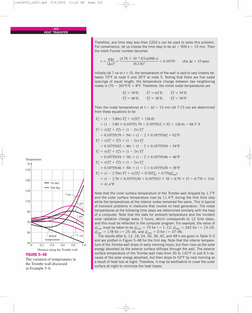
302HEAT TRANSFER

Therefore, any time step less than 2202 s can be used to solve this problem.For convenience, let us choose the time step to be �t � 900 s � 15 min. Thenthe mesh Fourier number becomes

� � � � 0.10755 (for �t � 15 min)

Initially (at 7 AM or t � 0), the temperature of the wall is said to vary linearly be-tween 70°F at node 0 and 30°F at node 5. Noting that there are five nodalspacings of equal length, the temperature change between two neighboringnodes is (70 � 30)°F/5 � 8°F. Therefore, the initial nodal temperatures are

� 70°F, � 62°F, � 54°F,

� 46°F, � 38°F, � 30°F

Then the nodal temperatures at t � �t � 15 min (at 7:15 AM) are determinedfrom these equations to be

� (1 � 3.80�) � �(2 � 126.0)

� (1 � 3.80 � 0.10755) 70 � 0.10755(2 � 62 � 126.0) � 68.3° F

� �( � ) � (1 � 2�)

� 0.10755(70 � 54) � (1 � 2 � 0.10755)62 � 62°F

� �( � ) � (1 � 2�)

� 0.10755(62 � 46) � (1 � 2 � 0.10755)54 � 54°F

� �( � ) � (1 � 2�)

� 0.10755(54 � 38) � (1 � 2 � 0.10755)46 � 46°F

� �( � ) � (1 � 2�)

� 0.10755(46 � 30) � (1 � 2 � 0.10755)38 � 38°F

� (1 � 2.70�) � �(2 � 0.70 � 0.770q· )

� (1 � 2.70 � 0.10755)30 � 0.10755(2 � 38 � 0.70 � 33 � 0.770 � 114)

� 41.4°F

Note that the inner surface temperature of the Trombe wall dropped by 1.7°Fand the outer surface temperature rose by 11.4°F during the first time stepwhile the temperatures at the interior nodes remained the same. This is typicalof transient problems in mediums that involve no heat generation. The nodaltemperatures at the following time steps are determined similarly with the helpof a computer. Note that the data for ambient temperature and the incidentsolar radiation change every 3 hours, which corresponds to 12 time steps,and this must be reflected in the computer program. For example, the value ofq· must be taken to be q· � 75 for i � 1–12, q· � 242 for i � 13–24,q· � 178 for i � 25–36, and q· � 0 for i � 37–96.

The results after 6, 12, 18, 24, 30, 36, 42, and 48 h are given in Table 5–5and are plotted in Figure 5–48 for the first day. Note that the interior tempera-ture of the Trombe wall drops in early morning hours, but then rises as the solarenergy absorbed by the exterior surface diffuses through the wall. The exteriorsurface temperature of the Trombe wall rises from 30 to 142°F in just 6 h be-cause of the solar energy absorbed, but then drops to 53°F by next morning asa result of heat loss at night. Therefore, it may be worthwhile to cover the outersurface at night to minimize the heat losses.

isolar

isolar

isolar

isolar

isolar

0solarT 0

outT 04T 0

5T 15

T 04T 0

5T 03T 1

4

T 03T 0

4T 02T 1

3

T 02T 0

3T 01T 1

2

T 01T 0

2T 00T 1

1

T 01T 0

0T 10

T 05T 0

4T 03

T 02T 0

1T 00

(4.78 � 10�6 ft2/s)(900 s)

(0.2 ft)2

α�t(�x)2

150

170

130

110

90

70

50

30

Temperature

Initialtemperature

7 AM

1 PM

1 AM

7 PM

°F

1 ft0.80.60.4

Distance along the Trombe wall

0.20

1st day

2nd day

FIGURE 5–48The variation of temperatures inthe Trombe wall discussedin Example 5–6.

cen58933_ch05.qxd 9/4/2002 11:42 AM Page 302

CHAPTER 5303

The rate of heat transfer from the Trombe wall to the interior of the house dur-ing each time step is determined from Newton’s law using the average temper-ature at the inner surface of the wall (node 0) as

Q � Q·

�t � hin A( � Tin) �t � hin A[( � )/2 � Tin]�t

Therefore, the amount of heat transfer during the first time step (i � 1) orduring the first 15-min period is

Q � hin A[( � )/2 � Tin] �t

� (1.8 Btu/h · ft2 · °F)(10 � 25 ft2)[(68.3 � 70)/2 � 70°F](0.25 h)

� �95.6 Btu

The negative sign indicates that heat is transferred to the Trombe wall from theair in the house, which represents a heat loss. Then the total heat transfer dur-ing a specified time period is determined by adding the heat transfer amountsfor each time step as

QTrombe wall � Q·

� hin A[( � )/2 � Tin] �t (5-55)

where I is the total number of time intervals in the specified time period. In thiscase I � 48 for 12 h, 96 for 24 h, and so on. Following the approach describedhere using a computer, the amount of heat transfer between the Trombe walland the interior of the house is determined to be

QTrombe wall � �17, 048 Btu after 12 h (�17, 078 Btu during the first 12 h)

QTrombe wall � �2483 Btu after 24 h (14, 565 Btu during the second 12 h)

QTrombe wall � 5610 Btu after 36 h (8093 Btu during the third 12 h)

QTrombe wall � 34, 400 Btu after 48 h (28, 790 Btu during the fourth 12 h)

Therefore, the house loses 2483 Btu through the Trombe wall the first day as aresult of the low start-up temperature but delivers a total of 36,883 Btu of heatto the house the second day. It can be shown that the Trombe wall will delivereven more heat to the house during the third day since it will start the day at ahigher average temperature.

T i�10T i

0�I

i�1

iTrombe wall�

I

i�1

T 00T 1

01Trombe wall

T i�10T i

0T i0

iTrombe wall

iTrombe wall

TABLE 5–5

The temperatures at the nodes of a Trombe wall at various times

Nodal Temperatures, °FTime Time Step, i T0 T1 T2 T3 T4 T5

0 h (7 AM) 0 70.0 62.0 54.0 46.0 38.0 30.06 h (1 PM) 24 65.3 61.7 61.5 69.7 94.1 142.0

12 h (7 PM) 48 71.6 74.2 80.4 88.4 91.7 82.418 h (1 AM) 72 73.3 75.9 77.4 76.3 71.2 61.224 h (7 AM) 96 71.2 71.9 70.9 67.7 61.7 53.030 h (1 PM) 120 70.3 71.1 74.3 84.2 108.3 153.236 h (7 PM) 144 75.4 81.1 89.4 98.2 101.0 89.742 h (1 AM) 168 75.8 80.7 83.5 83.0 77.4 66.248 h (7 AM) 192 73.0 75.1 72.2 66.0 66.0 56.3

cen58933_ch05.qxd 9/4/2002 11:42 AM Page 303

Two-Dimensional Transient Heat ConductionConsider a rectangular region in which heat conduction is significant in the x- and y-directions, and consider a unit depth of �z � 1 in the z-direction.Heat may be generated in the medium at a rate of g·(x, y, t), which may varywith time and position, with the thermal conductivity k of the medium as-sumed to be constant. Now divide the x-y-plane of the region into a rectangu-lar mesh of nodal points spaced �x and �y apart in the x- and y-directions,respectively, and consider a general interior node (m, n) whose coordinates arex � m�x and y � n�y, as shown in Figure 5–49. Noting that the volume ele-ment centered about the general interior node (m, n) involves heat conductionfrom four sides (right, left, top, and bottom) and the volume of the element isVelement � �x � �y � 1 � �x�y, the transient finite difference formulation fora general interior node can be expressed on the basis of Eq. 5–39 as

k�y � k�x � k�y

� k�x � g·m, n �x�y � �x�y C (5-56)

Taking a square mesh (�x � �y � l ) and dividing each term by k gives aftersimplifying,

Tm � 1, n � Tm � 1, n � Tm, n � 1 � Tm, n � 1 � 4Tm, n � � (5-57)

where again � � k/ C is the thermal diffusivity of the material and � � ��t/l 2

is the dimensionless mesh Fourier number. It can also be expressed in terms ofthe temperatures at the neighboring nodes in the following easy-to-rememberform:

Tleft � Ttop � Tright � Tbottom � 4Tnode � � (5-58)

Again the left side of this equation is simply the finite difference formulationof the problem for the steady case, as expected. Also, we are still not com-mitted to explicit or implicit formulation since we did not indicate the timestep on the left side of the equation. We now obtain the explicit finite differ-ence formulation by expressing the left side at time step i as

� � (5-59)

Expressing the left side at time step i � 1 instead of i would give the implicitformulation. This equation can be solved explicitly for the new temperature

to give

� �( ) � (1 � 4�) � � (5-60)

for all interior nodes (m, n) where m � 1, 2, 3, . . . , M � 1 and n � 1, 2,3, . . . , N � 1 in the medium. In the case of no heat generation and � � , the1

4

g· inodel 2

kT i

nodeT ileft � T i

top � T iright � T i

bottomT i�1node

T i�1node

T i�1node � T i

node

�g· i

nodel 2

kT i

left � T itop � T i

right � T ibottom � 4T i

node

T i�1node � T i

node

�g·nodel 2

k

T i�1m � T i

m

�g·m, nl 2

k

T i�1m � T i

m

�t

Tm, n�1 � Tm, n

�y

Tm�1, n � Tm, n

�x

Tm, n�1 � Tm, n

�y

Tm�1, n � Tm, n

�x

304HEAT TRANSFER

n – 1

n

n + 1

m – 1 m m + 1

∆x∆x

m, n

Volumeelement

m + 1, n

m, n + 1

m, n – 1

m – 1, ngm, n·

∆y

∆y

y

x

FIGURE 5–49The volume element of ageneral interior node (m, n) for two-dimensional transient conductionin rectangular coordinates.

cen58933_ch05.qxd 9/4/2002 11:42 AM Page 304

explicit finite difference formulation for a general interior node reduces to� ( )/4, which has the interpretation that the

temperature of an interior node at the new time step is simply the averageof the temperatures of its neighboring nodes at the previous time step(Fig. 5–50).

The stability criterion that requires the coefficient of in the expres-sion to be greater than or equal to zero for all nodes is equally valid for two-or three-dimensional cases and severely limits the size of the time step �t thatcan be used with the explicit method. In the case of transient two-dimensionalheat transfer in rectangular coordinates, the coefficient of in the ex-pression is 1 � 4�, and thus the stability criterion for all interior nodes in thiscase is 1 � 4� � 0, or

� � � (5-61)

where �x � �y � l. When the material of the medium and thus its thermaldiffusivity � are known and the value of the mesh size l is specified, thelargest allowable value of the time step �t can be determined from the relationabove. Again the boundary nodes involving convection and/or radiation aremore restrictive than the interior nodes and thus require smaller time steps.Therefore, the most restrictive boundary node should be used in the determi-nation of the maximum allowable time step �t when a transient problem issolved with the explicit method.

The application of Eq. 5–60 to each of the (M � 1) � (N � 1) interior nodesgives (M � 1) � (N � 1) equations. The remaining equations are obtained byapplying the method to the boundary nodes unless, of course, the boundarytemperatures are specified as being constant. The development of the transientfinite difference formulation of boundary nodes in two- (or three-) dimen-sional problems is similar to the development in the one-dimensional case dis-cussed earlier. Again the region is partitioned between the nodes by formingvolume elements around the nodes, and an energy balance is written for eachboundary node on the basis of Eq. 5–39. This is illustrated in Example 5–7.

(interior nodes, two-dimensional heattransfer in rectangular coordinates)

14

��tl 2

T i�1mT i

m

T i�1mT i

m

T ileft � T i

top � T iright � T i

bottomT i�1node

CHAPTER 5305

20°C

Time step i:

30°C

40°C

Node m

10°C

Tmi

25°C

Time step i + 1:

Node m

Tmi + 1

FIGURE 5–50In the case of no heat generationand � � , the temperature of an

interior node at the new time step isthe average of the temperatures of

its neighboring nodes at theprevious time step.

14

EXAMPLE 5–7 Transient Two-Dimensional Heat Conductionin L-Bars

Consider two-dimensional transient heat transfer in an L-shaped solid body thatis initially at a uniform temperature of 90°C and whose cross section is givenin Figure 5–51. The thermal conductivity and diffusivity of the body are k �15 W/m · °C and � � 3.2 � 10�6 m2/s, respectively, and heat is generated inthe body at a rate of g· � 2 � 106 W/m3. The left surface of the body is insu-lated, and the bottom surface is maintained at a uniform temperature of 90°Cat all times. At time t � 0, the entire top surface is subjected to convection toambient air at T� � 25°C with a convection coefficient of h � 80 W/m2 · °C,and the right surface is subjected to heat flux at a uniform rate of q·R � 5000W/m2. The nodal network of the problem consists of 15 equally spaced nodeswith �x � �y � 1.2 cm, as shown in the figure. Five of the nodes are at the bot-tom surface, and thus their temperatures are known. Using the explicit method,determine the temperature at the top corner (node 3) of the body after 1, 3, 5,10, and 60 min.

12 13 14 151110

6 7 8 954

321

x

y

∆x ∆x ∆x ∆x ∆x

∆y

∆y

90°C

qR·

∆x = ∆y = l

Convectionh, T�

FIGURE 5–51Schematic and nodal network for

Example 5–7.

cen58933_ch05.qxd 9/4/2002 11:42 AM Page 305

306HEAT TRANSFER

SOLUTION This is a transient two-dimensional heat transfer problem in rec-tangular coordinates, and it was solved in Example 5–3 for the steady case.Therefore, the solution of this transient problem should approach the solutionfor the steady case when the time is sufficiently large. The thermal conductiv-ity and heat generation rate are given to be constants. We observe that all nodesare boundary nodes except node 5, which is an interior node. Therefore, we willhave to rely on energy balances to obtain the finite difference equations. The re-gion is partitioned among the nodes equitably as shown in the figure, and theexplicit finite difference equations are determined on the basis of the energybalance for the transient case expressed as

Q· i � G

·� Velement C

The quantities h, T�, g· , and q·R do not change with time, and thus we do notneed to use the superscript i for them. Also, the energy balance expressions aresimplified using the definitions of thermal diffusivity � � k/ C and the dimen-sionless mesh Fourier number � � ��t/l2, where �x � �y � l.

(a) Node 1. (Boundary node subjected to convection and insulation, Fig.5–52a)

h (T� � ) � k � k

� g·1 � C

Dividing by k/4 and simplifying,

(T� � ) � 2( � ) � 2( � ) � �

which can be solved for to give

� 1 � 4� � 2� � 2� � � T� �

(b) Node 2. (Boundary node subjected to convection, Fig. 5–52b)

h�x(T� � ) � k � k�x

� k � g·2 �x � �x C

Dividing by k/2, simplifying, and solving for gives

� 1 � 4� � 2� � � � � 2 � T� �g·2l 2

k �2hlk

T i5T i

3T i1�T i

2hlk ��T i�1

2

T i�12

T i�12 � T i

2

�t

�y2

�y2

T i1 � T i

2

�x

�y2

T i5 � T i

2

�y

T i3 � T i

2

�x

�y2

T i2

g·1l 2

2k �hlk

T i4T i

2�T i1

hlk ��T i�1

1

T i�11

T i�11 � T i

1�

g·1l 2

kT i

1T i4T i

1T i2T i

12hlk

T i�11 � T i

1

�t

�y2

�x2

�y2

�x2

T i4 � T i

1

�y�x2

T i2 � T i

1

�x

�y2

T i1

�x2

T i�1m � T i

m

�tielement�

All sides

h, T�

1

4

2

(a) Node 1

h, T�

21

5

3

(b) Node 2


cen58933_ch05.qxd 9/4/2002 11:42 AM Page 306

CHAPTER 5307

(c) Node 3. (Boundary node subjected to convection on two sides, Fig. 5–53a)

h (T� � ) � k

� k � g·3 �


� 1 � 4� � 4� � 2� � � 2 T� �

(d ) Node 4. (On the insulated boundary, and can be treated as an interior node,Fig. 5–53b). Noting that T10 � 90°C, Eq. 5–60 gives

� (1 � 4�) � � � 2 � 90 �

(e) Node 5. (Interior node, Fig. 5–54a). Noting that T11 � 90°C, Eq. 5–60gives

� (1 � 4�) � � � � � 90 �

(f ) Node 6. (Boundary node subjected to convection on two sides, Fig. 5–54b)

h (T� � ) � k � k�x � k�y

� � g·6 � C

Dividing by 3k/4, simplifying, and solving for gives

� 1 � 4� � 4�

� 2 � 4 � 2 � 4 � 90 � 4 T� � 3

(g) Node 7. (Boundary node subjected to convection, Fig. 5–55)

h�x(T� � ) � k � k�x

� k � g·7�x � �x C


� 1 � 4� � 2� � � � � 2 � 90 � T� �g·7l 2

k �2hlkT i

8T i6�T i

7hlk ��T i�1

7

T i�17

T i�17 � T i

7

�t

�y2

�y2

T i6 � T i

7

�x

�y2

T i13 � T i

7

�y

T i8 � T i

7

�x

�y2

T i7

g·6l 2

k �hlk

T i7T i

5T i3

�3�

T i3

hl3k ��T i�1

6

T i�16

T i�16 � T i

6

�t

3�x�y4

3�x�y4

T i3 � T i

6

�y�x2

T i5 � T i

6

�x

T i12 � T i

6

�y

T i7 � T i

6

�x

�y2

T i6��x

2�

�y2 �

g·5l 2

k �T i6T i

4T i2�T i

5T i�15

g·4l 2

k �T i5T i

1�T i4T i�1

4

g·3l 2

2k �hlk

T i6T i

4�T i3

hlk ��T i�1

3

T i�13

T i�13 � T i

3

�t

�y2

�x2

�y2

�x2

T i2 � T i

3

�x

�y2

T i6 � T i

3

�y�x2

T i3��x

2�

�y2 �

h, T�

h, T�

3

6

2

(a) Node 3

(5)

10

1Mirror

54

(b) Node 4



h, T�

(a) Node 5

5

12

3

76

(b) Node 6

4

11

2

65



h, T�h, T�

9

1513

876

qR·



cen58933_ch05.qxd 9/4/2002 11:42 AM Page 307

308HEAT TRANSFER

(h) Node 8. This node is identical to node 7, and the finite difference formula-tion of this node can be obtained from that of node 7 by shifting the node num-bers by 1 (i.e., replacing subscript m by subscript m � 1). It gives

� 1 � 4� � 2� � � � � 2 � 90 � T� �

(i ) Node 9. (Boundary node subjected to convection on two sides, Fig. 5–55)

h (T� � ) � q·R k

� � g·9 � C


� 1 � 4� � 2� � 2� � 90 � � T� �

This completes the finite difference formulation of the problem. Next we needto determine the upper limit of the time step �t from the stability criterion,which requires the coefficient of in the expression (the primary coeffi-cient) to be greater than or equal to zero for all nodes. The smallest primary co-efficient in the nine equations here is the coefficient of in the expression,and thus the stability criterion for this problem can be expressed as

1 � 4� � 4� � 0 → � � → �t �

since � � ��t /l 2. Substituting the given quantities, the maximum allowablevalue of the time step is determined to be

�t � � 10.6 s

Therefore, any time step less than 10.6 s can be used to solve this problem. Forconvenience, let us choose the time step to be �t � 10 s. Then the meshFourier number becomes

� � � � 0.222 (for �t � 10 s)

Substituting this value of � and other given quantities, the developed transientfinite difference equations simplify to

� 0.0836 � 0.444( � � 11.2)

� 0.0836 � 0.222( � � 2 � 22.4)

� 0.0552 � 0.444( � � 12.8)

� 0.112 � 0.222( � 2 � 109.2)

� 0.112 � 0.222( � � � 109.2)T i6T i

4T i2T i

1T i�15

T i5T i

1T i4T i�1

4

T i6T i

2T i3T i�1

3

T i5T i

3T i1T i

2T i�12

T i4T i

2T i1T i�1

1

(3.2 � 10�6 m2/s)(10 s)

(0.012 m)2

��tl 2

(0.012 m)2

4(3.2 � 10�6 m2/s)[1 � (80 W/m2 · °C)(0.012 m)/(15 W/m · °C)]

l 2

4�(1 � hl/k)1

4(1 � hl/k)hlk

T i3

T i�1mT i

m

g·9l 2

2k �hlk

q·R lk

T i8�T i

9hlk ��T i�1

9

T i�19

T i�19 � T i

9

�t

�y2

�x2

�y2

�x2

T i8 � T i

9

�x

k�y2

T i15 � T i

9

�y�x2

�y2

T i9

�x2

g·8l 2

k �2hlkT i

9T i7�T i

8hlk ��T i�1

8

cen58933_ch05.qxd 9/4/2002 11:42 AM Page 308

CHAPTER 5309

� 0.0931 � 0.074(2 � 4 � 2 � 424)

� 0.0836 � 0.222( � � 202.4)

� 0.0836 � 0.222( � � 202.4)

� 0.0836 � 0.444( � 105.2)

Using the specified initial condition as the solution at time t � 0 (for i � 0),sweeping through these nine equations will give the solution at intervals of10 s. The solution at the upper corner node (node 3) is determined to be100.2, 105.9, 106.5, 106.6, and 106.6°C at 1, 3, 5, 10, and 60 min, re-spectively. Note that the last three solutions are practically identical to thesolution for the steady case obtained in Example 5–3. This indicates that steadyconditions are reached in the medium after about 5 min.

T i8T i

9T i�19

T i9T i

7T i8T i�1

8

T i8T i

6T i7T i�1

7

T i7T i

5T i3T i

6T i�16

TOPIC OF SPECIAL INTEREST

Controlling the Numerical Error

A comparison of the numerical results with the exact results for tempera-ture distribution in a cylinder would show that the results obtained by a nu-merical method are approximate, and they may or may not be sufficientlyclose to the exact (true) solution values. The difference between a numeri-cal solution and the exact solution is the error involved in the numericalsolution, and it is primarily due to two sources:

• The discretization error (also called the truncation or formulationerror), which is caused by the approximations used in the formulationof the numerical method.

• The round-off error, which is caused by the computer’s use of alimited number of significant digits and continuously rounding (orchopping) off the digits it cannot retain.

Below we discuss both types of errors.

Discretization ErrorThe discretization error involved in numerical methods is due to replacingthe derivatives by differences in each step, or the actual temperature distri-bution between two adjacent nodes by a straight line segment.

Consider the variation of the solution of a transient heat transfer problemwith time at a specified nodal point. Both the numerical and actual (exact)solutions coincide at the beginning of the first time step, as expected, butthe numerical solution deviates from the exact solution as the time t in-creases. The difference between the two solutions at t � �t is due to the ap-proximation at the first time step only and is called the local discretizationerror. One would expect the situation to get worse with each step since thesecond step uses the erroneous result of the first step as its starting pointand adds a second local discretization error on top of it, as shown in Figure5–56. The accumulation of the local discretization errors continues with theincreasing number of time steps, and the total discretization error at any

T(xm, t)

Globalerror

Localerror

Actual solutionT(x0, t)

T0

t0 t1 t2 t3

T1

T2

T3 Numericalsolution

Time

Step 1 Step 2 Step 3

FIGURE 5–56The local and global discretization

errors of the finite differencemethod at the third time step

at a specified nodal point.

cen58933_ch05.qxd 9/4/2002 11:42 AM Page 309

310HEAT TRANSFER

step is called the global or accumulated discretization error. Note that thelocal and global discretization errors are identical for the first time step.The global discretization error usually increases with the increasing num-ber of steps, but the opposite may occur when the solution functionchanges direction frequently, giving rise to local discretization errors of op-posite signs, which tend to cancel each other.

To have an idea about the magnitude of the local discretization error,consider the Taylor series expansion of the temperature at a specified nodalpoint m about time ti,

T(xm, ti � �t) � T(xm, ti) � �t � �t 2 � · · · (5-62)

The finite difference formulation of the time derivative at the same nodalpoint is expressed as

� � (5-63)

or

T(xm, ti � �t) � T(xm, ti) � �t (5-64)

which resembles the Taylor series expansion terminated after the first twoterms. Therefore, the third and later terms in the Taylor series expansionrepresent the error involved in the finite difference approximation. For asufficiently small time step, these terms decay rapidly as the order of de-rivative increases, and their contributions become smaller and smaller. Thefirst term neglected in the Taylor series expansion is proportional to �t 2,and thus the local discretization error of this approximation, which is theerror involved in each step, is also proportional to �t 2.

The local discretization error is the formulation error associated with asingle step and gives an idea about the accuracy of the method used. How-ever, the solution results obtained at every step except the first one involvethe accumulated error up to that point, and the local error alone does nothave much significance. What we really need to know is the global dis-cretization error. At the worst case, the accumulated discretization errorafter I time steps during a time period t0 is i(�t)2 � (t0/�t)(�t)2 � t0�t,which is proportional to �t. Thus, we conclude that the local discretizationerror is proportional to the square of the step size �t 2 while the global dis-cretization error is proportional to the step size �t itself. Therefore, thesmaller the mesh size (or the size of the time step in transient problems),the smaller the error, and thus the more accurate is the approximation. Forexample, halving the step size will reduce the global discretization error byhalf. It should be clear from the discussions above that the discretization er-ror can be minimized by decreasing the step size in space or time as muchas possible. The discretization error approaches zero as the differencequantities such as �x and �t approach the differential quantities such as dxand dt.

�T(xm, ti)�t

T i�1m � T i

m

�t

T(xm, ti � �t) � T(xm, ti)

�t

�T(xm, ti)�t

�2T(xm, ti)

�t2

12

�T(xm, ti)�t

cen58933_ch05.qxd 9/4/2002 11:42 AM Page 310

CHAPTER 5311

Round-off ErrorIf we had a computer that could retain an infinite number of digits for allnumbers, the difference between the exact solution and the approximate(numerical) solution at any point would entirely be due to discretization er-ror. But we know that every computer (or calculator) represents numbersusing a finite number of significant digits. The default value of the numberof significant digits for many computers is 7, which is referred to as singleprecision. But the user may perform the calculations using 15 significantdigits for the numbers, if he or she wishes, which is referred to as doubleprecision. Of course, performing calculations in double precision will re-quire more computer memory and a longer execution time.

In single precision mode with seven significant digits, a computer willregister the number 44444.666666 as 44444.67 or 44444.66, depending onthe method of rounding the computer uses. In the first case, the excess dig-its are said to be rounded to the closest integer, whereas in the second casethey are said to be chopped off. Therefore, the numbers a � 44444.12345and b � 44444.12032 are equivalent for a computer that performs calcula-tions using seven significant digits. Such a computer would give a � b �0 instead of the true value 0.00313.

The error due to retaining a limited number of digits during calculationsis called the round-off error. This error is random in nature and there is noeasy and systematic way of predicting it. It depends on the number of cal-culations, the method of rounding off, the type of computer, and even thesequence of calculations.

In algebra you learned that a � b � c � a � c � b, which seems quitereasonable. But this is not necessarily true for calculations performed witha computer, as demonstrated in Figure 5–57. Note that changing the se-quence of calculations results in an error of 30.8 percent in just two opera-tions. Considering that any significant problem involves thousands or evenmillions of such operations performed in sequence, we realize that the ac-cumulated round-off error has the potential to cause serious error withoutgiving any warning signs. Experienced programmers are very much awareof this danger, and they structure their programs to prevent any buildup ofthe round-off error. For example, it is much safer to multiply a number by10 than to add it 10 times. Also, it is much safer to start any additionprocess with the smallest numbers and continue with larger numbers. Thisrule is particularly important when evaluating series with a large number ofterms with alternating signs.

The round-off error is proportional to the number of computations per-formed during the solution. In the finite difference method, the number ofcalculations increases as the mesh size or the time step size decreases.Halving the mesh or time step size, for example, will double the number ofcalculations and thus the accumulated round-off error.

Controlling the Error in Numerical MethodsThe total error in any result obtained by a numerical method is the sum ofthe discretization error, which decreases with decreasing step size, and theround-off error, which increases with decreasing step size, as shown in Fig-ure 5–58. Therefore, decreasing the step size too much in order to get more

Given:

a � 7777777

b � �7777776

c � 0.4444432

Find: D � a � b � c

E � a � c � b

Solution:

D � 7777777 � 7777776 � 0.4444432

� 1 � 0.4444432

� 1.444443 (Correct result)

E � 7777777 � 0.4444432 � 7777776

� 7777777 � 7777776

� 1.000000 (In error by 30.8%)

FIGURE 5–57A simple arithmetic operation

performed with a computerin single precision using seven

significant digits, which results in30.8 percent error when the order

of operation is reversed.

Totalerror

Discretizationerror

Round-off error

Error

Step sizeOptimumstep size

FIGURE 5–58As the mesh or time step size

decreases, the discretization errordecreases but the round-off

error increases.

cen58933_ch05.qxd 9/4/2002 11:42 AM Page 311

312HEAT TRANSFER

accurate results may actually backfire and give less accurate results be-cause of a faster increase in the round-off error. We should be careful not tolet round-off error get out of control by avoiding a large number of compu-tations with very small numbers.

In practice, we will not know the exact solution of the problem, and thuswe will not be able to determine the magnitude of the error involved in thenumerical method. Knowing that the global discretization error is propor-tional to the step size is not much help either since there is no easy way ofdetermining the value of the proportionality constant. Besides, the globaldiscretization error alone is meaningless without a true estimate of theround-off error. Therefore, we recommend the following practical proce-dures to assess the accuracy of the results obtained by a numerical method.

• Start the calculations with a reasonable mesh size �x (and time stepsize �t for transient problems) based on experience. Then repeat thecalculations using a mesh size of �x/2. If the results obtained byhalving the mesh size do not differ significantly from the resultsobtained with the full mesh size, we conclude that the discretizationerror is at an acceptable level. But if the difference is larger than wecan accept, then we have to repeat the calculations using a mesh size�x/4 or even a smaller one at regions of high temperature gradients.We continue in this manner until halving the mesh size does not causeany significant change in the results, which indicates that thediscretization error is reduced to an acceptable level.

• Repeat the calculations using double precision holding the mesh size(and the size of the time step in transient problems) constant. If thechanges are not significant, we conclude that the round-off error is nota problem. But if the changes are too large to accept, then we may tryreducing the total number of calculations by increasing the mesh sizeor changing the order of computations. But if the increased mesh sizegives unacceptable discretization errors, then we may have to find areasonable compromise.

It should always be kept in mind that the results obtained by any numer-ical method may not reflect any trouble spots in certain problems that re-quire special consideration such as hot spots or areas of high temperaturegradients. The results that seem quite reasonable overall may be in consid-erable error at certain locations. This is another reason for always repeatingthe calculations at least twice with different mesh sizes before acceptingthem as the solution of the problem. Most commercial software packageshave built-in routines that vary the mesh size as necessary to obtain highlyaccurate solutions. But it is a good engineering practice to be aware of anypotential pitfalls of numerical methods and to examine the results obtainedwith a critical eye.

SUMMARY

Analytical solution methods are limited to highly simplifiedproblems in simple geometries, and it is often necessary to use

a numerical method to solve real world problems with com-plicated geometries or nonuniform thermal conditions. The

cen58933_ch05.qxd 9/4/2002 11:42 AM Page 312

CHAPTER 5313

numerical finite difference method is based on replacing deriv-atives by differences, and the finite difference formulation of aheat transfer problem is obtained by selecting a sufficient num-ber of points in the region, called the nodal points or nodes,and writing energy balances on the volume elements centeredabout the nodes.

For steady heat transfer, the energy balance on a volume el-ement can be expressed in general as

Q·

� g·Velement � 0

whether the problem is one-, two-, or three-dimensional. Forconvenience in formulation, we always assume all heat trans-fer to be into the volume element from all surfaces toward thenode under consideration, except for specified heat flux whosedirection is already specified. The finite difference formula-tions for a general interior node under steady conditions are ex-pressed for some geometries as follows:

One-dimensional steady conduction � � 0in a plane wall:

Two-dimensional steady

Tleft � Ttop � Tright � Tbottom � 4Tnode � � 0conduction in rectangular coordinates:

where �x is the nodal spacing for the plane wall and �x ��y � l is the nodal spacing for the two-dimensional case. Insu-lated boundaries can be viewed as mirrors in formulation, andthus the nodes on insulated boundaries can be treated as inte-rior nodes by using mirror images.

The finite difference formulation at node 0 at the left bound-ary of a plane wall for steady one-dimensional heat conductioncan be expressed as

Q·

left surface � kA � g·0(A�x/2) � 0

where A�x/2 is the volume of the volume, g·0 is the rate of heatgeneration per unit volume at x � 0, and A is the heat transferarea. The form of the first term depends on the boundary con-dition at x � 0 (convection, radiation, specified heat flux, etc.).

The finite difference formulation of heat conduction prob-lems usually results in a system of N algebraic equations in Nunknown nodal temperatures that need to be solved simultane-ously. There are numerous systematic approaches available inthe literature. Several widely available equation solvers can

also be used to solve a system of equations simultaneously atthe press of a button.

The finite difference formulation of transient heat conduc-tion problems is based on an energy balance that also accountsfor the variation of the energy content of the volume elementduring a time interval �t. The heat transfer and heat generationterms are expressed at the previous time step i in the explicitmethod, and at the new time step i � 1 in the implicit method.For a general node m, the finite difference formulations areexpressed as

Explicitmethod:

Q· i � G

·� Velement C

Implicitmethod:

Q· i�1 � G

·� Velement C

where and are the temperatures of node m at timesti � i�t and ti�1 � (i � 1)�t, respectively, and � rep-resents the temperature change of the node during the time in-terval �t between the time steps i and i � 1. The explicit andimplicit formulations given here are quite general and can beused in any coordinate system regardless of heat transfer beingone-, two-, or three-dimensional.

The explicit formulation of a general interior node for one-and two-dimensional heat transfer in rectangular coordinatescan be expressed as

One-dimen- � �( � ) � (1 � 2�) � �sional case:

Two-� �( � � � )

dimen-sional

� (1 � 4�) � �case:

where

� �

is the dimensionless mesh Fourier number and � � k/ C is thethermal diffusivity of the medium.

The implicit method is inherently stable, and any value of �tcan be used with that method as the time step. The largest valueof the time step �t in the explicit method is limited by the sta-bility criterion, expressed as: the coefficients of all in the

expressions (called the primary coefficients) must begreater than or equal to zero for all nodes m. The maximumvalue of �t is determined by applying the stability criterion tothe equation with the smallest primary coefficient since it is the

T i�1m

T im

��t�x2

g· inodel 2

kT i

node

T ibottomT i

rightT itopT i

leftT i�1node

g· im�x2

kT i

mT im�1T i

m�1T i�1m

T imT i�1

m

T i�1mT i

m

T i�1m � T i

m

�ti�1element�

All sides

T i�1m � T i

m

�tielement�

All sides

T1 � T0

�x

g·nodel 2

k

g·mk

Tm�1 � 2Tm � Tm�1

(�x)2

�All sides

cen58933_ch05.qxd 9/4/2002 11:42 AM Page 313

314HEAT TRANSFER

most restrictive. For problems with specified temperatures orheat fluxes at all the boundaries, the stability criterion can be

expressed as � � for one-dimensional problems and � � forthe two-dimensional problems in rectangular coordinates.

14

12

REFERENCES AND SUGGESTED READING

1. D. A. Anderson, J. C. Tannehill, and R. H. Pletcher.Computational Fluid Mechanics and Heat Transfer. NewYork: Hemisphere, 1984.

2. C. A. Brebbia. The Boundary Element Method forEngineers. New York: Halsted Press, 1978.

3. G. E. Forsythe and W. R. Wasow. Finite DifferenceMethods for Partial Differential Equations. New York:John Wiley & Sons, 1960.

4. B. Gebhart. Heat Conduction and Mass Diffusion. NewYork: McGraw-Hill, 1993.

5. K. H. Huebner and E. A. Thornton. The Finite ElementMethod for Engineers. 2nd ed. New York: John Wiley &Sons, 1982.

6. Y. Jaluria and K. E. Torrance. Computational HeatTransfer. New York: Hemisphere, 1986.

7. W. J. Minkowycz, E. M. Sparrow, G. E. Schneider, andR. H. Pletcher. Handbook of Numerical Heat Transfer.New York: John Wiley & Sons, 1988.

8. G. E. Myers. Analytical Methods in Conduction HeatTransfer. New York: McGraw-Hill, 1971.

9. D. H. Norrie and G. DeVries. An Introduction to FiniteElement Analysis. New York: Academic Press, 1978.

10. M. N. Özisik. Finite Difference Methods in Heat Transfer.Boca Raton, FL: CRC Press, 1994.

11. S. V. Patankhar. Numerical Heat Transfer and Fluid Flow.New York: Hemisphere, 1980.

12. T. M. Shih. Numerical Heat Transfer. New York:Hemisphere, 1984.

PROBLEMS*

Why Numerical Methods?

5–1C What are the limitations of the analytical solutionmethods?

5–2C How do numerical solution methods differ from ana-lytical ones? What are the advantages and disadvantages ofnumerical and analytical methods?

5–3C What is the basis of the energy balance method? Howdoes it differ from the formal finite difference method? For aspecified nodal network, will these two methods result in thesame or a different set of equations?

5–4C Consider a heat conduction problem that can be solvedboth analytically, by solving the governing differential equa-tion and applying the boundary conditions, and numerically,by a software package available on your computer. Which

approach would you use to solve this problem? Explain yourreasoning.

5–5C Two engineers are to solve an actual heat transferproblem in a manufacturing facility. Engineer A makes the nec-essary simplifying assumptions and solves the problemanalytically, while engineer B solves it numerically using apowerful software package. Engineer A claims he solvedthe problem exactly and thus his results are better, while engi-neer B claims that he used a more realistic model and thus hisresults are better. To resolve the dispute, you are asked to solvethe problem experimentally in a lab. Which engineer do youthink the experiments will prove right? Explain.

Finite Difference Formulation of Differential Equations

5–6C Define these terms used in the finite difference formu-lation: node, nodal network, volume element, nodal spacing,and difference equation.

5–7 Consider three consecutive nodes n � 1, n, and n � 1 ina plane wall. Using the finite difference form of the first deriv-ative at the midpoints, show that the finite difference form ofthe second derivative can be expressed as

� 0Tn�1 � 2Tn � Tn�1

�x2

*Problems designated by a “C” are concept questions, andstudents are encouraged to answer them all. Problems designatedby an “E” are in English units, and the SI users can ignore them.Problems with an EES-CD icon are solved using EES, andcomplete solutions together with parametric studies are includedon the enclosed CD. Problems with a computer-EES icon arecomprehensive in nature, and are intended to be solved with acomputer, preferably using the EES software that accompaniesthis text.

cen58933_ch05.qxd 9/4/2002 11:42 AM Page 314

CHAPTER 5315

5–8 The finite difference formulation of steady two-dimensional heat conduction in a medium with heat generationand constant thermal conductivity is given by

�

� � 0

in rectangular coordinates. Modify this relation for the three-dimensional case.

5–9 Consider steady one-dimensional heat conduction in aplane wall with variable heat generation and constant thermalconductivity. The nodal network of the medium consists ofnodes 0, 1, 2, 3, and 4 with a uniform nodal spacing of �x.Using the finite difference form of the first derivative (not theenergy balance approach), obtain the finite difference formula-tion of the boundary nodes for the case of uniform heat flux q·0at the left boundary (node 0) and convection at the right bound-ary (node 4) with a convection coefficient of h and an ambienttemperature of T�.

5–10 Consider steady one-dimensional heat conduction in aplane wall with variable heat generation and constant thermalconductivity. The nodal network of the medium consists of

nodes 0, 1, 2, 3, 4, and 5 with a uniform nodal spacing of �x.Using the finite difference form of the first derivative (not theenergy balance approach), obtain the finite difference formula-tion of the boundary nodes for the case of insulation at the leftboundary (node 0) and radiation at the right boundary (node 5)with an emissivity of and surrounding temperature of Tsurr.

One-Dimensional Steady Heat Conduction

5–11C Explain how the finite difference form of a heat con-duction problem is obtained by the energy balance method.

5–12C In the energy balance formulation of the finite differ-ence method, it is recommended that all heat transfer at theboundaries of the volume element be assumed to be into thevolume element even for steady heat conduction. Is this a validrecommendation even though it seems to violate the conserva-tion of energy principle?

5–13C How is an insulated boundary handled in the finitedifference formulation of a problem? How does a symmetryline differ from an insulated boundary in the finite differenceformulation?

5–14C How can a node on an insulated boundary be treatedas an interior node in the finite difference formulation of aplane wall? Explain.

5–15C Consider a medium in which the finite differenceformulation of a general interior node is given in its simplestform as

� � 0

(a) Is heat transfer in this medium steady or transient?(b) Is heat transfer one-, two-, or three-dimensional?(c) Is there heat generation in the medium?(d) Is the nodal spacing constant or variable?(e) Is the thermal conductivity of the medium constant or

variable?

5–16 Consider steady heat conduction in a plane wall whoseleft surface (node 0) is maintained at 30°C while the right sur-face (node 8) is subjected to a heat flux of 800 W/m2. Expressthe finite difference formulation of the boundary nodes 0 and 8

g·m

kTm�1 � 2Tm � Tm�1

�x2

g·m, n

k

Tm, n�1 � 2Tm, n � Tm, n�1

�y2

Tm�1, n � 2Tm, n � Tm�1, n

�x2

n – 1 n n + 1

Tn – 1

T(x)

∆x

Tn + 1

Tn

∆x

x

FIGURE P5–7

∆x

Insulation

Radiation

ε

Tsurr

0 1 2 3 4 5

g(x)·

FIGURE P5–10

∆x

30°C

800

0 1 2 3 4 5 6 7 8

No heat generation W—–m2

FIGURE P5–16

cen58933_ch05.qxd 9/4/2002 11:42 AM Page 315

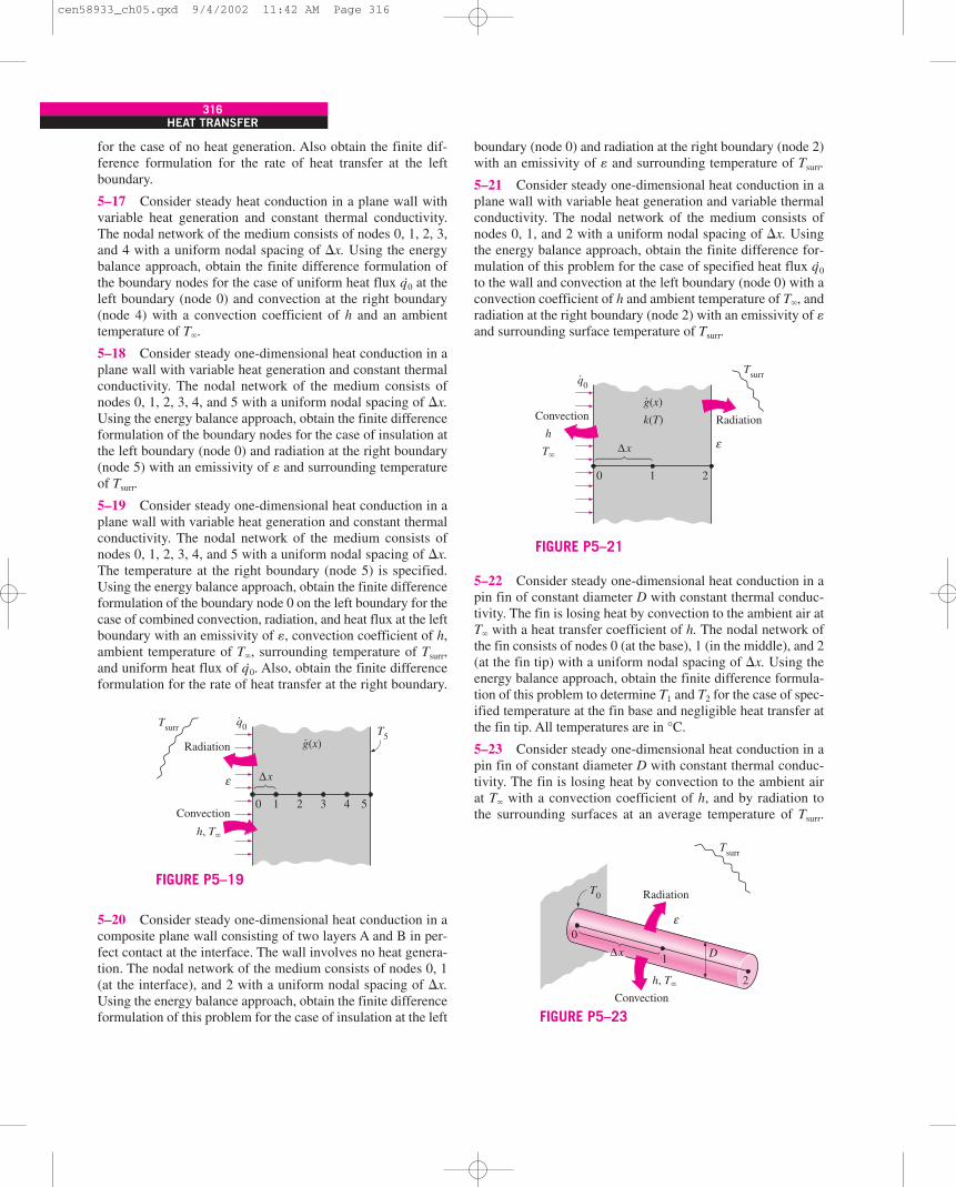
316HEAT TRANSFER

for the case of no heat generation. Also obtain the finite dif-ference formulation for the rate of heat transfer at the leftboundary.

5–17 Consider steady heat conduction in a plane wall withvariable heat generation and constant thermal conductivity.The nodal network of the medium consists of nodes 0, 1, 2, 3,and 4 with a uniform nodal spacing of �x. Using the energybalance approach, obtain the finite difference formulation ofthe boundary nodes for the case of uniform heat flux q·0 at theleft boundary (node 0) and convection at the right boundary(node 4) with a convection coefficient of h and an ambienttemperature of T�.

5–18 Consider steady one-dimensional heat conduction in aplane wall with variable heat generation and constant thermalconductivity. The nodal network of the medium consists ofnodes 0, 1, 2, 3, 4, and 5 with a uniform nodal spacing of �x.Using the energy balance approach, obtain the finite differenceformulation of the boundary nodes for the case of insulation atthe left boundary (node 0) and radiation at the right boundary(node 5) with an emissivity of and surrounding temperatureof Tsurr.

5–19 Consider steady one-dimensional heat conduction in aplane wall with variable heat generation and constant thermalconductivity. The nodal network of the medium consists ofnodes 0, 1, 2, 3, 4, and 5 with a uniform nodal spacing of �x.The temperature at the right boundary (node 5) is specified.Using the energy balance approach, obtain the finite differenceformulation of the boundary node 0 on the left boundary for thecase of combined convection, radiation, and heat flux at the leftboundary with an emissivity of , convection coefficient of h,ambient temperature of T�, surrounding temperature of Tsurr,and uniform heat flux of q·0. Also, obtain the finite differenceformulation for the rate of heat transfer at the right boundary.

5–20 Consider steady one-dimensional heat conduction in acomposite plane wall consisting of two layers A and B in per-fect contact at the interface. The wall involves no heat genera-tion. The nodal network of the medium consists of nodes 0, 1(at the interface), and 2 with a uniform nodal spacing of �x.Using the energy balance approach, obtain the finite differenceformulation of this problem for the case of insulation at the left

boundary (node 0) and radiation at the right boundary (node 2)with an emissivity of and surrounding temperature of Tsurr.

5–21 Consider steady one-dimensional heat conduction in aplane wall with variable heat generation and variable thermalconductivity. The nodal network of the medium consists ofnodes 0, 1, and 2 with a uniform nodal spacing of �x. Usingthe energy balance approach, obtain the finite difference for-mulation of this problem for the case of specified heat flux q·0to the wall and convection at the left boundary (node 0) with aconvection coefficient of h and ambient temperature of T�, andradiation at the right boundary (node 2) with an emissivity of and surrounding surface temperature of Tsurr.

5–22 Consider steady one-dimensional heat conduction in apin fin of constant diameter D with constant thermal conduc-tivity. The fin is losing heat by convection to the ambient air atT� with a heat transfer coefficient of h. The nodal network ofthe fin consists of nodes 0 (at the base), 1 (in the middle), and 2(at the fin tip) with a uniform nodal spacing of �x. Using theenergy balance approach, obtain the finite difference formula-tion of this problem to determine T1 and T2 for the case of spec-ified temperature at the fin base and negligible heat transfer atthe fin tip. All temperatures are in °C.

5–23 Consider steady one-dimensional heat conduction in apin fin of constant diameter D with constant thermal conduc-tivity. The fin is losing heat by convection to the ambient airat T� with a convection coefficient of h, and by radiation tothe surrounding surfaces at an average temperature of Tsurr.

∆x

Radiation

Convection

h, T�

ε

T5

0 1 2 3 4 5

g(x)·

Tsurrq0·

FIGURE P5–19

∆x

Convection Radiationh

T�ε

0 1 2

g(x)

k(T)

·

Tsurrq0·

FIGURE P5–21

0

1∆x

Radiation

h, T�

T0

D

ε

Convection

2

Tsurr

FIGURE P5–23

cen58933_ch05.qxd 9/4/2002 11:42 AM Page 316

CHAPTER 5317

The nodal network of the fin consists of nodes 0 (at the base),1 (in the middle), and 2 (at the fin tip) with a uniform nodalspacing of �x. Using the energy balance approach, obtain thefinite difference formulation of this problem to determineT1 and T2 for the case of specified temperature at the fin baseand negligible heat transfer at the fin tip. All temperaturesare in °C.

5–24 Consider a large uranium plate of thickness 5 cm andthermal conductivity k � 28 W/m · °C in which heat is gener-ated uniformly at a constant rate of g· � 6 � 105 W/m3. Oneside of the plate is insulated while the other side is subjectedto convection to an environment at 30°C with a heat transfercoefficient of h � 60 W/m2 · °C. Considering six equallyspaced nodes with a nodal spacing of 1 cm, (a) obtain the finitedifference formulation of this problem and (b) determine thenodal temperatures under steady conditions by solving thoseequations.

5–25 Consider an aluminum alloy fin (k � 180 W/m · °C) oftriangular cross section whose length is L � 5 cm, base thick-ness is b � 1 cm, and width w in the direction normal to theplane of paper is very large. The base of the fin is maintainedat a temperature of T0 � 180°C. The fin is losing heat by con-vection to the ambient air at T� � 25°C with a heat transfercoefficient of h � 25 W/m2 · °C and by radiation to the sur-rounding surfaces at an average temperature of Tsurr � 290 K.Using the finite difference method with six equally spacednodes along the fin in the x-direction, determine (a) the tem-peratures at the nodes and (b) the rate of heat transfer from thefin for w � 1 m. Take the emissivity of the fin surface to be 0.9and assume steady one-dimensional heat transfer in the fin.

5–26 Reconsider Problem 5–25. Using EES (or other)software, investigate the effect of the fin base

temperature on the fin tip temperature and the rate of heattransfer from the fin. Let the temperature at the fin base vary

from 100°C to 200°C. Plot the fin tip temperature and the rateof heat transfer as a function of the fin base temperature, anddiscuss the results.

5–27 Consider a large plane wall of thickness L � 0.4 m,thermal conductivity k � 2.3 W/m · °C, and surface areaA � 20 m2. The left side of the wall is maintained at a constanttemperature of 80°C, while the right side loses heat by con-vection to the surrounding air at T� � 15°C with a heat trans-fer coefficient of h � 24 W/m2 · °C. Assuming steady one-dimensional heat transfer and taking the nodal spacing to be10 cm, (a) obtain the finite difference formulation for all nodes,(b) determine the nodal temperatures by solving those equa-tions, and (c) evaluate the rate of heat transfer through the wall.

5–28 Consider the base plate of a 800-W household iron hav-ing a thickness of L � 0.6 cm, base area of A � 160 cm2, andthermal conductivity of k � 20 W/m · °C. The inner surface ofthe base plate is subjected to uniform heat flux generated bythe resistance heaters inside. When steady operating conditionsare reached, the outer surface temperature of the plate is mea-sured to be 85°C. Disregarding any heat loss through the upperpart of the iron and taking the nodal spacing to be 0.2 cm,(a) obtain the finite difference formulation for the nodes and(b) determine the inner surface temperature of the plate bysolving those equations. Answer: (b) 100°C

5–29 Consider a large plane wall of thickness L � 0.3 m,thermal conductivity k � 2.5 W/m · °C, and surface areaA � 12 m2. The left side of the wall is subjected to a heat fluxof q·0 � 700 W/m2 while the temperature at that surface is mea-sured to be T0 � 60°C. Assuming steady one-dimensional heattransfer and taking the nodal spacing to be 6 cm, (a) obtain thefinite difference formulation for the six nodes and (b) deter-mine the temperature of the other surface of the wall by solv-ing those equations.

5–30E A large steel plate having a thickness of L � 5 in.,thermal conductivity of k � 7.2 Btu/h · ft · °F, and an emissiv-ity of � 0.6 is lying on the ground. The exposed surface of

θ1

23

45

0

∆x

L

wh, T�

T0

x

b

Triangular fin

tan =θ b/2—–L

FIGURE P5–25

1 20

160 cm2

3 x

Base plate85°C

∆x = 0.2 cm

Insulation

Resistance heater, 800 W

FIGURE P5–28

cen58933_ch05.qxd 9/4/2002 11:42 AM Page 317

318HEAT TRANSFER

the plate exchanges heat by convection with the ambient airat T� � 80°F with an average heat transfer coefficient ofh � 3.5 Btu/h · ft2 · °F as well as by radiation with the open skyat an equivalent sky temperature of Tsky � 510 R. The groundtemperature below a certain depth (say, 3 ft) is not affected bythe weather conditions outside and remains fairly constant at50°F at that location. The thermal conductivity of the soil canbe taken to be ksoil � 0.49 Btu/h · ft · °F, and the steel plate canbe assumed to be in perfect contact with the ground. Assumingsteady one-dimensional heat transfer and taking the nodalspacings to be 1 in. in the plate and 0.6 ft in the ground, (a) ob-tain the finite difference formulation for all 11 nodes shown inFigure P5–30E and (b) determine the top and bottom surfacetemperatures of the plate by solving those equations.

5–31E Repeat Problem 5–30E by disregarding radiation heattransfer from the upper surface. Answers: (b) 78.7°F, 78.4°F

5–32 Consider a stainless steel spoon (k � 15.1 W/m · C, � 0.6) that is partially immersed in boiling water at 95°C ina kitchen at 25°C. The handle of the spoon has a cross sectionof about 0.2 cm � 1 cm and extends 18 cm in the air from thefree surface of the water. The spoon loses heat by convectionto the ambient air with an average heat transfer coefficient ofh � 13 W/m2 · °C as well as by radiation to the surroundingsurfaces at an average temperature of Tsurr � 295 K. Assumingsteady one-dimensional heat transfer along the spoon and tak-ing the nodal spacing to be 3 cm, (a) obtain the finite differenceformulation for all nodes, (b) determine the temperature of thetip of the spoon by solving those equations, and (c) determinethe rate of heat transfer from the exposed surfaces of the spoon.

5–33 Repeat Problem 5–32 using a nodal spacing of 1.5 cm.

5–34 Reconsider Problem 5–33. Using EES (or other)software, investigate the effects of the thermal

conductivity and the emissivity of the spoon material on thetemperature at the spoon tip and the rate of heat transfer fromthe exposed surfaces of the spoon. Let the thermal conductiv-ity vary from 10 W/m · °C to 400 W/m · °C, and the emissivityfrom 0.1 to 1.0. Plot the spoon tip temperature and the heattransfer rate as functions of thermal conductivity and emissiv-ity, and discuss the results.

5–35 One side of a 2-m-high and 3-m-wide vertical plateat 130°C is to be cooled by attaching aluminum fins (k �237 W/m · °C) of rectangular profile in an environment at35°C. The fins are 2 cm long, 0.3 cm thick, and 0.4 cm apart.The heat transfer coefficient between the fins and the sur-rounding air for combined convection and radiation is esti-mated to be 30 W/m2 · °C. Assuming steady one-dimensionalheat transfer along the fin and taking the nodal spacing to be0.5 cm, determine (a) the finite difference formulation of thisproblem, (b) the nodal temperatures along the fin by solvingthese equations, (c) the rate of heat transfer from a single fin,

x

0

5

6

7

8

9

10

1234

Plate

Radiation

Convection

Tsky

εh, T�

1 in.

0.6 ft

Soil

FIGURE P5–30E

Tsurr = 295 K

3 cm

0

95°

18 cm

6

5

4321

T� = 25°C

h = 13 W/m2·°C

FIGURE P5–32

0.4cm

0.3cm

2 cm3 m

1

0

2

0.5 cm

3 4

130°CT� = 35°C

x

FIGURE P5–35

cen58933_ch05.qxd 9/4/2002 11:42 AM Page 318

CHAPTER 5319

and (d) the rate of heat transfer from the entire finned surfaceof the plate.

5–36 A hot surface at 100°C is to be cooled by attach-ing 3-cm-long, 0.25-cm-diameter aluminum pin fins (k �237 W/m · °C) with a center-to-center distance of 0.6 cm. Thetemperature of the surrounding medium is 30°C, and the com-bined heat transfer coefficient on the surfaces is 35 W/m2 · °C.Assuming steady one-dimensional heat transfer along the finand taking the nodal spacing to be 0.5 cm, determine (a) the fi-nite difference formulation of this problem, (b) the nodal tem-peratures along the fin by solving these equations, (c) the rateof heat transfer from a single fin, and (d) the rate of heat trans-fer from a 1-m � 1-m section of the plate.

5–37 Repeat Problem 5–36 using copper fins (k � 386W/m · °C) instead of aluminum ones.

Answers: (b) 98.6°C, 97.5°C, 96.7°C, 96.0°C, 95.7°C, 95.5°C

5–38 Two 3-m-long and 0.4-cm-thick cast iron (k � 52W/m · °C, � 0.8) steam pipes of outer diameter 10 cm areconnected to each other through two 1-cm-thick flanges ofouter diameter 20 cm, as shown in the figure. The steam flowsinside the pipe at an average temperature of 200°C with a heattransfer coefficient of 180 W/m2 · °C. The outer surface of thepipe is exposed to convection with ambient air at 8°C with aheat transfer coefficient of 25 W/m2 · °C as well as radiationwith the surrounding surfaces at an average temperature ofTsurr � 290 K. Assuming steady one-dimensional heat conduc-tion along the flanges and taking the nodal spacing to be 1 cmalong the flange (a) obtain the finite difference formulation forall nodes, (b) determine the temperature at the tip of the flangeby solving those equations, and (c) determine the rate of heattransfer from the exposed surfaces of the flange.

5–39 Reconsider Problem 5–38. Using EES (or other)software, investigate the effects of the steam tem-

perature and the outer heat transfer coefficient on the flange tiptemperature and the rate of heat transfer from the exposed sur-faces of the flange. Let the steam temperature vary from 150°Cto 300°C and the heat transfer coefficient from 15 W/m2 · °C to60 W/m2 · °C. Plot the flange tip temperature and the heattransfer rate as functions of steam temperature and heat trans-fer coefficient, and discuss the results.

5–40 Using EES (or other) software, solve these sys-tems of algebraic equations.

(a) 3x1 � x2 � 3x3 � 0

�x1 � 2x2 � x3 � 3

2x1 � x2 � x3 � 2

(b) 4x1 � 2x � 0.5x3 � �2

x � x2 � x3 � 11.964

x1 � x2 � x3 � 3Answers: (a) x1 � 2, x2 � 3, x3 � �1, (b) x1 � 2.33, x2 � 2.29,

x3 � �1.62


(a) 3x1 � 2x2 � x3 � x4 � 6

x1 � 2x2 � x4 � �3

�2x1 � x2 � 3x3 � x4 � 2

3x2 � x3 � 4x4 � �6

(b) 3x1 � x � 2x3 � 8

�x � 3x2 � 2x3 � �6.293

2x1 � x � 4x3 � �1242

21

22

31

22

10 2 3

0.5 cm100°C

3 cm

0.6cm

0.25cm

4 5 6x

FIGURE P5–36

Tair = 8°C

Steam200°C

9.2 cm

1 cm1 cm

10 cm

20 cm

FIGURE P5–38

cen58933_ch05.qxd 9/4/2002 11:42 AM Page 319

320HEAT TRANSFER


(a) 4x1 � x2 � 2x3 � x4 � �6

x1 � 3x2 � x3 � 4x4 � �1

�x1 � 2x2 � 5x4 � 5

2x2 � 4x3 � 3x4 � �5

(b) 2x1 � x � 2x3 � x4 � 1

x � 4x2 � 2x � 2x4 � �3

�x1 � x � 5x3 � 10

3x1 � x � 8x4 � 15

Two-Dimensional Steady Heat Conduction


Tleft � Ttop � Tright � Tbottom � 4Tnode � � 0


variable?


Tnode � (Tleft � Ttop � Tright � Tbottom)/4


variable?

5–45C What is an irregular boundary? What is a practicalway of handling irregular boundary surfaces with the finite dif-ference method?

5–46 Consider steady two-dimensional heat transfer in a longsolid body whose cross section is given in the figure. The tem-peratures at the selected nodes and the thermal conditions atthe boundaries are as shown. The thermal conductivity of thebody is k � 45 W/m · °C, and heat is generated in the body uni-formly at a rate of g· � 6 � 106 W/m3. Using the finite differ-ence method with a mesh size of �x � �y � 5.0 cm, determine(a) the temperatures at nodes 1, 2, and 3 and (b) the rate of heatloss from the bottom surface through a 1-m-long section of thebody.

5–47 Consider steady two-dimensional heat transfer in a longsolid body whose cross section is given in the figure. The mea-sured temperatures at selected points of the outer surfaces areas shown. The thermal conductivity of the body is k � 45W/m · °C, and there is no heat generation. Using the finite dif-ference method with a mesh size of �x � �y � 2.0 cm, deter-mine the temperatures at the indicated points in the medium.Hint: Take advantage of symmetry.

5–48 Consider steady two-dimensional heat transfer in a longsolid bar whose cross section is given in the figure. The mea-sured temperatures at selected points of the outer surfaces areas shown. The thermal conductivity of the body is k � 20W/m · °C, and there is no heat generation. Using the finite dif-ference method with a mesh size of �x � �y � 1.0 cm, deter-mine the temperatures at the indicated points in the medium.

Answers: T1 � 185°C, T2 � T3 � T4 � 190°C

5–49 Starting with an energy balance on a volume element,obtain the steady two-dimensional finite difference equationfor a general interior node in rectangular coordinates for T(x, y)for the case of variable thermal conductivity and uniform heatgeneration.

g·nodel 2

k

23

42

23

21

42

2

1

3

5 cm5 cm

240

Convection

T� = 20°C, h = 50 W/m2 · °C

325

350°C305

290

260

200°C

Insulation

g = 6 × 106 W/m3·

FIGURE P5–46

7 8 9

4 5 6

1 2 3

200 180 150180150

200 180 150°C180150

180180

200200

180180

2 cm2 cm

FIGURE P5–47

cen58933_ch05.qxd 9/4/2002 11:42 AM Page 320

CHAPTER 5321

5–50 Consider steady two-dimensional heat transfer in a longsolid body whose cross section is given in the figure. The tem-peratures at the selected nodes and the thermal conditions onthe boundaries are as shown. The thermal conductivity of thebody is k � 180 W/m · °C, and heat is generated in the bodyuniformly at a rate of g· � 107 W/m3. Using the finite differencemethod with a mesh size of �x � �y � 10 cm, determine(a) the temperatures at nodes 1, 2, 3, and 4 and (b) the rateof heat loss from the top surface through a 1-m-long section ofthe body.

5–51 Reconsider Problem 5–50. Using EES (or other)software, investigate the effects of the thermal

conductivity and the heat generation rate on the temperatures atnodes 1 and 3, and the rate of heat loss from the top surface.Let the thermal conductivity vary from 10 W/m · °C to 400W/m · °C and the heat generation rate from 105 W/m3 to 108

W/m3. Plot the temperatures at nodes 1 and 3, and the rate ofheat loss as functions of thermal conductivity and heat genera-tion rate, and discuss the results.

5–52 Consider steady two-dimensional heat transfer in a longsolid bar whose cross section is given in the figure. The mea-sured temperatures at selected points on the outer surfaces areas shown. The thermal conductivity of the body is k � 20W/m · °C, and there is no heat generation. Using the finite dif-ference method with a mesh size of �x � �y � 1.0 cm, deter-mine the temperatures at the indicated points in the medium.Hint: Take advantage of symmetry.

Answers: (b) T1 � T4 � 143°C, T2 � T3 � 136°C

5–53 Consider steady two-dimensional heat transfer in anL-shaped solid body whose cross section is given in the figure.The thermal conductivity of the body is k � 45 W/m · °C, andheat is generated in the body at a rate of g· � 5 � 106 W/m3.

1

3

2

4

200°C180

Insulation

(a)

Insulation

(b)

Insu

latio

n

150

180

200

1 2

3 4

100120 120

100°C

120 120

140 140

FIGURE P5–48

3 4

1 2

200 200200200

100 100°C100100

150150

120120

0.1 m

0.1 m

g = 107 W/m3·

FIGURE P5–50

Insulation

(a)

4

2

5 6

3

1

150 150

200

250

300

200 1 cm

1 cm250

300

100°C

yx

(b)

21 3 4

100 100 100 100°C

200

Insu

latio

n

Insu

latio

n

200

100

200 200 200°C

1 cm1 cm

FIGURE P5–52

1 2 3

Convection

4 5 6 7 8

1.5cm

1.5cm

Insu

latio

nqL·

120°C

h, T�

FIGURE P5–53

cen58933_ch05.qxd 9/4/2002 11:42 AM Page 321

322HEAT TRANSFER

The right surface of the body is insulated, and the bottom sur-face is maintained at a uniform temperature of 120°C. Theentire top surface is subjected to convection with ambient airat T� � 30°C with a heat transfer coefficient of h � 55W/m2 · °C, and the left surface is subjected to heat flux at a uni-form rate of q·L � 8000 W/m2. The nodal network of the prob-lem consists of 13 equally spaced nodes with �x � �y �1.5 cm. Five of the nodes are at the bottom surface and thustheir temperatures are known. (a) Obtain the finite differenceequations at the remaining eight nodes and (b) determine thenodal temperatures by solving those equations.

5–54E Consider steady two-dimensional heat transfer in along solid bar of square cross section in which heat is gener-ated uniformly at a rate of g· � 0.19 � 105 Btu/h · ft3. The crosssection of the bar is 0.4 ft � 0.4 ft in size, and its thermal con-ductivity is k � 16 Btu/h · ft · °F. All four sides of the bar aresubjected to convection with the ambient air at T� � 70°F witha heat transfer coefficient of h � 7.9 Btu/h · ft2 · °F. Using thefinite difference method with a mesh size of �x � �y � 0.2 ft,determine (a) the temperatures at the nine nodes and (b) therate of heat loss from the bar through a 1-ft-long section.

Answer: (b) 3040 Btu/h

5–55 Hot combustion gases of a furnace are flowing througha concrete chimney (k � 1.4 W/m · °C) of rectangular cross

section. The flow section of the chimney is 20 cm � 40 cm,and the thickness of the wall is 10 cm. The average temperatureof the hot gases in the chimney is Ti � 280°C, and the averageconvection heat transfer coefficient inside the chimney is hi �75 W/m2 · °C. The chimney is losing heat from its outer surfaceto the ambient air at To � 15°C by convection with a heattransfer coefficient of ho � 18 W/m2 · °C and to the sky byradiation. The emissivity of the outer surface of the wall is � 0.9, and the effective sky temperature is estimated to be250 K. Using the finite difference method with �x � �y �10 cm and taking full advantage of symmetry, (a) obtain thefinite difference formulation of this problem for steady two-dimensional heat transfer, (b) determine the temperatures at thenodal points of a cross section, and (c) evaluate the rate of heatloss for a 1-m-long section of the chimney.

5–56 Repeat Problem 5–55 by disregarding radiation heattransfer from the outer surfaces of the chimney.

5–57 Reconsider Problem 5–55. Using EES (or other)software, investigate the effects of hot-gas tem-

perature and the outer surface emissivity on the temperatures atthe outer corner of the wall and the middle of the inner surfaceof the right wall, and the rate of heat loss. Let the temperatureof the hot gases vary from 200°C to 400°C and the emissivityfrom 0.1 to 1.0. Plot the temperatures and the rate of heat lossas functions of the temperature of the hot gases and the emis-sivity, and discuss the results.

5–58 Consider a long concrete dam (k � 0.6 W/m · °C,�s � 0.7 m2/s) of triangular cross section whose

exposed surface is subjected to solar heat flux of q·s �800 W/m2 and to convection and radiation to the environ-ment at 25°C with a combined heat transfer coefficient of 30W/m2 · °C. The 2-m-high vertical section of the dam is sub-jected to convection by water at 15°C with a heat transfercoefficient of 150 W/m2 · °C, and heat transfer through the2-m-long base is considered to be negligible. Using the finitedifference method with a mesh size of �x � �y � 1 m andassuming steady two-dimensional heat transfer, determine thetemperature of the top, middle, and bottom of the exposed sur-face of the dam. Answers: 21.3°C, 43.2°C, 43.6°C

321

654

987

h, T�h, T�

h, T�

h, T�

g·

FIGURE P5–54E

10 cm

20 cm

10 cm40 cm

10 cm

10 cm

Chimney

Hot gases

Ti, hi

To, ho ε

Tsky

FIGURE P5–55

3

54

2

1 m

Water 1 m

1 m 1 m

6

1

qs·

h

T�

FIGURE P5–58

cen58933_ch05.qxd 9/4/2002 11:43 AM Page 322

CHAPTER 5323

5–59E Consider steady two-dimensional heat transfer in aV-grooved solid body whose cross section is given in the fig-ure. The top surfaces of the groove are maintained at 32°Fwhile the bottom surface is maintained at 212°F. The side sur-faces of the groove are insulated. Using the finite differencemethod with a mesh size of �x � �y � 1 ft and taking advan-tage of symmetry, determine the temperatures at the middle ofthe insulated surfaces.

5–60 Reconsider Problem 5–59E. Using EES (orother) software, investigate the effects of the

temperatures at the top and bottom surfaces on the temperaturein the middle of the insulated surface. Let the temperatures atthe top and bottom surfaces vary from 32°F to 212°F. Plot thetemperature in the middle of the insulated surface as functionsof the temperatures at the top and bottom surfaces, and discussthe results.

5–61 Consider a long solid bar whose thermal conductivity isk � 12 W/m · °C and whose cross section is given in the figure.The top surface of the bar is maintained at 50°C while the bot-tom surface is maintained at 120°C. The left surface is insu-lated and the remaining three surfaces are subjected toconvection with ambient air at T� � 25°C with a heat transfercoefficient of h � 30 W/m2 · °C. Using the finite differencemethod with a mesh size of �x � �y � 10 cm, (a) obtain thefinite difference formulation of this problem for steady two-

dimensional heat transfer and (b) determine the unknown nodaltemperatures by solving those equations.

Answers: (b) 85.7°C, 86.4°C, 87.6°C

5–62 Consider a 5-m-long constantan block (k � 23W/m · °C) 30 cm high and 50 cm wide. The block is com-pletely submerged in iced water at 0°C that is well stirred, andthe heat transfer coefficient is so high that the temperatures onboth sides of the block can be taken to be 0°C. The bottom sur-face of the bar is covered with a low-conductivity material sothat heat transfer through the bottom surface is negligible. Thetop surface of the block is heated uniformly by a 6-kW resis-tance heater. Using the finite difference method with a meshsize of �x � �y � 10 cm and taking advantage of symmetry,(a) obtain the finite difference formulation of this problem forsteady two-dimensional heat transfer, (b) determine the un-known nodal temperatures by solving those equations, and(c) determine the rate of heat transfer from the block to the icedwater.

Transient Heat Conduction

5–63C How does the finite difference formulation of a transient heat conduction problem differ from that of asteady heat conduction problem? What does the term A�xC( � )/�t represent in the transient finite differ-ence formulation?

5–64C What are the two basic methods of solution of tran-sient problems based on finite differencing? How do heattransfer terms in the energy balance formulation differ in thetwo methods?

5–65C The explicit finite difference formulation of a generalinterior node for transient heat conduction in a plane wall isgiven by

� 2 � � �

Obtain the finite difference formulation for the steady case bysimplifying the relation above.

T i�1m � T i

m

�g· i

m �x2

kT i

m�1T imT i

m�1

T imT i�1

m

212°F

1 ft

3

2

1

Insu

latio

n

Insu

latio

n5

4

32°F

6 8

7

11

10

9

1 ft

FIGURE P5–59E

10 cmInsu

latio

n

10 cm

120°C

50°C

Convection

h, T�

FIGURE P5–61

Insulation

Insulation

6 kW heater

0°C0°C

10cm10cm

FIGURE P5–62

cen58933_ch05.qxd 9/4/2002 11:43 AM Page 323

324HEAT TRANSFER

5–66C The explicit finite difference formulation of a generalinterior node for transient two-dimensional heat conduction isgiven by

� �( � � � )

� (1 � 4�) � �

Obtain the finite difference formulation for the steady case bysimplifying the relation above.

5–67C Is there any limitation on the size of the time step �tin the solution of transient heat conduction problems using(a) the explicit method and (b) the implicit method?

5–68C Express the general stability criterion for the explicitmethod of solution of transient heat conduction problems.

5–69C Consider transient one-dimensional heat conductionin a plane wall that is to be solved by the explicit method. Ifboth sides of the wall are at specified temperatures, express thestability criterion for this problem in its simplest form.

5–70C Consider transient one-dimensional heat conductionin a plane wall that is to be solved by the explicit method.If both sides of the wall are subjected to specified heat flux, express the stability criterion for this problem in its sim-plest form.

5–71C Consider transient two-dimensional heat conductionin a rectangular region that is to be solved by the explicitmethod. If all boundaries of the region are either insulated or atspecified temperatures, express the stability criterion for thisproblem in its simplest form.

5–72C The implicit method is unconditionally stable andthus any value of time step �t can be used in the solution oftransient heat conduction problems. To minimize the computa-tion time, someone suggests using a very large value of �tsince there is no danger of instability. Do you agree with thissuggestion? Explain.

5–73 Consider transient heat conduction in a plane wallwhose left surface (node 0) is maintained at 50°C while theright surface (node 6) is subjected to a solar heat flux of 600W/m2. The wall is initially at a uniform temperature of 50°C.Express the explicit finite difference formulation of the bound-ary nodes 0 and 6 for the case of no heat generation. Also,obtain the finite difference formulation for the total amountof heat transfer at the left boundary during the first threetime steps.

5–74 Consider transient heat conduction in a plane wall withvariable heat generation and constant thermal conductivity.The nodal network of the medium consists of nodes 0, 1, 2, 3,and 4 with a uniform nodal spacing of �x. The wall is initiallyat a specified temperature. Using the energy balance approach,obtain the explicit finite difference formulation of the boundarynodes for the case of uniform heat flux q·0 at the left boundary

(node 0) and convection at the right boundary (node 4) with aconvection coefficient of h and an ambient temperature of T�.Do not simplify.

5–75 Repeat Problem 5–74 for the case of implicit formula-tion.

5–76 Consider transient heat conduction in a plane wall withvariable heat generation and constant thermal conductivity.The nodal network of the medium consists of nodes 0, 1, 2,3, 4, and 5 with a uniform nodal spacing of �x. The wall is ini-tially at a specified temperature. Using the energy balance ap-proach, obtain the explicit finite difference formulation of theboundary nodes for the case of insulation at the left boundary(node 0) and radiation at the right boundary (node 5) with anemissivity of and surrounding temperature of Tsurr.

5–77 Consider transient heat conduction in a plane wall withvariable heat generation and constant thermal conductivity.The nodal network of the medium consists of nodes 0, 1, 2, 3,and 4 with a uniform nodal spacing of �x. The wall is initiallyat a specified temperature. The temperature at the right bound-ary (node 4) is specified. Using the energy balance approach,obtain the explicit finite difference formulation of the boundarynode 0 for the case of combined convection, radiation, and heatflux at the left boundary with an emissivity of , convection co-efficient of h, ambient temperature of T�, surrounding temper-ature of Tsurr, and uniform heat flux of q·0 toward the wall. Also,obtain the finite difference formulation for the total amount ofheat transfer at the right boundary for the first 20 time steps.

g· inodel 2

kT i

node

T ibottomT i

rightT itopT i

leftT i�1node

∆x

h, T�

0 1 2 3 4

g(x, t )·

q0·

x

FIGURE P5–74

∆x

Radiation

Convection

h, T�

TL

0 1 2 3 4

L

g(x, t )·

Tsurr

q0·

x

FIGURE P5–77

cen58933_ch05.qxd 9/4/2002 11:43 AM Page 324

CHAPTER 5325

5–78 Starting with an energy balance on a volume element,obtain the two-dimensional transient explicit finite differenceequation for a general interior node in rectangular coordinatesfor T(x, y, t) for the case of constant thermal conductivity andno heat generation.

5–79 Starting with an energy balance on a volume element,obtain the two-dimensional transient implicit finite differenceequation for a general interior node in rectangular coordinatesfor T(x, y, t) for the case of constant thermal conductivity andno heat generation.

5–80 Starting with an energy balance on a disk volume ele-ment, derive the one-dimensional transient explicit finite dif-ference equation for a general interior node for T(z, t) in acylinder whose side surface is insulated for the case of constantthermal conductivity with uniform heat generation.

5–81 Consider one-dimensional transient heat conduction ina composite plane wall that consists of two layers A and B withperfect contact at the interface. The wall involves no heat gen-eration and initially is at a specified temperature. The nodalnetwork of the medium consists of nodes 0, 1 (at the interface),and 2 with a uniform nodal spacing of �x. Using the energybalance approach, obtain the explicit finite difference formula-tion of this problem for the case of insulation at the left bound-ary (node 0) and radiation at the right boundary (node 2) withan emissivity of and surrounding temperature of Tsurr.

5–82 Consider transient one-dimensional heat conduction ina pin fin of constant diameter D with constant thermal conduc-tivity. The fin is losing heat by convection to the ambient air atT� with a heat transfer coefficient of h and by radiation to thesurrounding surfaces at an average temperature of Tsurr. Thenodal network of the fin consists of nodes 0 (at the base), 1 (inthe middle), and 2 (at the fin tip) with a uniform nodal spacingof �x. Using the energy balance approach, obtain the explicitfinite difference formulation of this problem for the case of aspecified temperature at the fin base and negligible heat trans-fer at the fin tip.

5–83 Repeat Problem 5–82 for the case of implicitformulation.

5–84 Consider a large uranium plate of thickness L � 8 cm,thermal conductivity k � 28 W/m · °C, and thermal diffusivity� � 12.5 � 10�6 m2/s that is initially at a uniform temperatureof 100°C. Heat is generated uniformly in the plate at a constantrate of g· � 106 W/m3. At time t � 0, the left side of the plate isinsulated while the other side is subjected to convection withan environment at T� � 20°C with a heat transfer coefficient ofh � 35 W/m2 · °C. Using the explicit finite difference approachwith a uniform nodal spacing of �x � 2 cm, determine (a) thetemperature distribution in the plate after 5 min and (b) howlong it will take for steady conditions to be reached in the plate.

5–85 Reconsider Problem 5–84. Using EES (or other)software, investigate the effect of the cooling

time on the temperatures of the left and right sides of the plate.Let the time vary from 5 min to 60 min. Plot the temperaturesat the left and right surfaces as a function of time, and discussthe results.

5–86 Consider a house whose south wall consists of a 30-cm-thick Trombe wall whose thermal conductivity is k � 0.70W/m · °C and whose thermal diffusivity is � � 0.44 � 10�6

m2/s. The variations of the ambient temperature Tout and thesolar heat flux q·solar incident on a south-facing vertical surfacethroughout the day for a typical day in February are given inthe table in 3-h intervals. The Trombe wall has single glazingwith an absorptivity-transmissivity product of � � 0.76 (thatis, 76 percent of the solar energy incident is absorbed by theexposed surface of the Trombe wall), and the average com-bined heat transfer coefficient for heat loss from the Trombewall to the ambient is determined to be hout � 3.4 W/m2 · °C.The interior of the house is maintained at Tin � 20°C at alltimes, and the heat transfer coefficient at the interior surface ofthe Trombe wall is hin � 9.1 W/m2 · °C. Also, the vents on theTrombe wall are kept closed, and thus the only heat transfer be-tween the air in the house and the Trombe wall is through the

Radiation

ε

Tsurr

∆x

0 1 2

Insulation

Interface

∆x

BA

FIGURE P5–81

Sun’srays

Trombewall

Glazing

Heatgain

Heatloss

FIGURE P5–86

cen58933_ch05.qxd 9/4/2002 11:43 AM Page 325

326HEAT TRANSFER

interior surface of the wall. Assuming the temperature of theTrombe wall to vary linearly between 20°C at the interior sur-face and 0°C at the exterior surface at 7 AM and using the ex-plicit finite difference method with a uniform nodal spacing of�x � 5 cm, determine the temperature distribution along thethickness of the Trombe wall after 6, 12, 18, 24, 30, 36, 42, and48 hours and plot the results. Also, determine the net amount ofheat transferred to the house from the Trombe wall during thefirst day if the wall is 2.8 m high and 7 m long.

5–87 Consider two-dimensional transient heat transfer in anL-shaped solid bar that is initially at a uniform temperatureof 140°C and whose cross section is given in the figure. Thethermal conductivity and diffusivity of the body are k � 15W/m · °C and � � 3.2 � 10�6 m2/s, respectively, and heat isgenerated in the body at a rate of g· � 2 � 107 W/m3. The rightsurface of the body is insulated, and the bottom surface ismaintained at a uniform temperature of 140°C at all times. Attime t � 0, the entire top surface is subjected to convectionwith ambient air at T� � 25°C with a heat transfer coefficientof h � 80 W/m2 · °C, and the left surface is subjected touniform heat flux at a rate of q·L � 8000 W/m2. The nodal net-work of the problem consists of 13 equally spaced nodes with�x � �y � 1.5 cm. Using the explicit method, determine thetemperature at the top corner (node 3) of the body after 2, 5,and 30 min.

5–88 Reconsider Problem 5–87. Using EES (or other)software, plot the temperature at the top corner as

a function of heating time varies from 2 min to 30 min, and dis-cuss the results.

5–89 Consider a long solid bar (k � 28 W/m · °C and � �12 � 10�6 m2/s) of square cross section that is initially at a uni-form temperature of 20°C. The cross section of the bar is20 cm � 20 cm in size, and heat is generated in it uniformly ata rate of g· � 8 � 105 W/m3. All four sides of the bar are sub-jected to convection to the ambient air at T� � 30°C witha heat transfer coefficient of h � 45 W/m2 · °C. Using theexplicit finite difference method with a mesh size of �x ��y � 10 cm, determine the centerline temperature of the bar(a) after 10 min and (b) after steady conditions are established.

5–90E Consider a house whose windows are made of0.375-in.-thick glass (k � 0.48 Btu/h · ft · °F and � � 4.2 �10�6 ft2/s). Initially, the entire house, including the walls andthe windows, is at the outdoor temperature of To � 35°F. It isobserved that the windows are fogged because the indoor tem-perature is below the dew-point temperature of 54°F. Now theheater is turned on and the air temperature in the house israised to Ti � 72°F at a rate of 2°F rise per minute. The heattransfer coefficients at the inner and outer surfaces of the wallcan be taken to be hi � 1.2 and ho � 2.6 Btu/h · ft2 · °F, respec-tively, and the outdoor temperature can be assumed to remainconstant. Using the explicit finite difference method with amesh size of �x � 0.125 in., determine how long it will take

TABLE P5–86

The hourly variations of the monthly average ambienttemperature and solar heat flux incident on avertical surface

Ambient Solar Time of Day Temperature, °C Insolation, W/m2

7 AM–10 AM 0 37510 AM–1 PM 4 750

1 PM–4 PM 6 5804 PM–7 PM 1 957 PM–10 PM �2 0

10 PM–1 AM �3 01 AM–4 AM �4 04 AM–7 AM 4 0

1 2 3

Convection

4 5 6 7 8

1.5cm

1.5cm

Insu

latio

nqL·

140°C

h, T�

FIGURE P5–87

10 cm10 cm

321

654

987

h, T�h, T�

h, T�

h, T�

g·

FIGURE P5–89

0.375 inFog

House Outdoors21

∆x

3 4

Ti

hi

To

ho

Windowglass

FIGURE P5–90E

cen58933_ch05.qxd 9/4/2002 11:43 AM Page 326

CHAPTER 5327

for the fog on the windows to clear up (i.e., for the inner sur-face temperature of the window glass to reach 54°F).

5–91 A common annoyance in cars in winter months is theformation of fog on the glass surfaces that blocks the view.A practical way of solving this problem is to blow hot air or toattach electric resistance heaters to the inner surfaces. Considerthe rear window of a car that consists of a 0.4-cm-thick glass(k � 0.84 W/m · °C and � � 0.39 � 10�6 m2/s). Strip heaterwires of negligible thickness are attached to the inner surfaceof the glass, 4 cm apart. Each wire generates heat at a rate of10 W/m length. Initially the entire car, including its windows,is at the outdoor temperature of To � �3°C. The heat transfercoefficients at the inner and outer surfaces of the glass can betaken to be hi � 6 and ho � 20 W/m2 · °C, respectively. Usingthe explicit finite difference method with a mesh size of �x �0.2 cm along the thickness and �y � 1 cm in the direction nor-mal to the heater wires, determine the temperature distributionthroughout the glass 15 min after the strip heaters are turnedon. Also, determine the temperature distribution when steadyconditions are reached.

5–92 Repeat Problem 5–91 using the implicit methodwith a time step of 1 min.

5–93 The roof of a house consists of a 15-cm-thick concreteslab (k � 1.4 W/m · °C and � � 0.69 � 10�6 m2/s) that is 20 mwide and 20 m long. One evening at 6 PM, the slab is observedto be at a uniform temperature of 18°C. The average ambientair and the night sky temperatures for the entire night are pre-dicted to be 6°C and 260 K, respectively. The convection heattransfer coefficients at the inner and outer surfaces of the roofcan be taken to be hi � 5 and ho � 12 W/m2 · °C, respectively.The house and the interior surfaces of the walls and the floor

are maintained at a constant temperature of 20°C during thenight, and the emissivity of both surfaces of the concrete roofis 0.9. Considering both radiation and convection heat transfersand using the explicit finite difference method with a time stepof �t � 5 min and a mesh size of �x � 3 cm, determine thetemperatures of the inner and outer surfaces of the roof at 6 AM.Also, determine the average rate of heat transfer through theroof during that night.

5–94 Consider a refrigerator whose outer dimensions are1.80 m � 0.8 m � 0.7 m. The walls of the refrigerator areconstructed of 3-cm-thick urethane insulation (k � 0.026W/m · ° C and � � 0.36 � 10�6 m2/s) sandwiched betweentwo layers of sheet metal with negligible thickness. The refrig-erated space is maintained at 3°C and the average heat transfercoefficients at the inner and outer surfaces of the wall are6 W/m2 · °C and 9 W/m2 · °C, respectively. Heat transferthrough the bottom surface of the refrigerator is negligible. Thekitchen temperature remains constant at about 25°C. Initially,the refrigerator contains 15 kg of food items at an averagespecific heat of 3.6 kJ/kg · °C. Now a malfunction occurs andthe refrigerator stops running for 6 h as a result. Assuming the

Thermalsymmetry line

Outersurface

Innersurface

Glass

Thermalsymmetry line

Heater10 W/m

1 cm

0.2 cm

FIGURE P5–91

ε

ε

Concreteroof

15 cm

Radiation

Radiation

Convection

Convection

hi, Ti

Ti

ho, To

Tsky

FIGURE P5–93

Heat

25°C

hohi

Refrigerator

Air

3°C

Food15 kg

FIGURE P5–94

cen58933_ch05.qxd 9/4/2002 11:43 AM Page 327

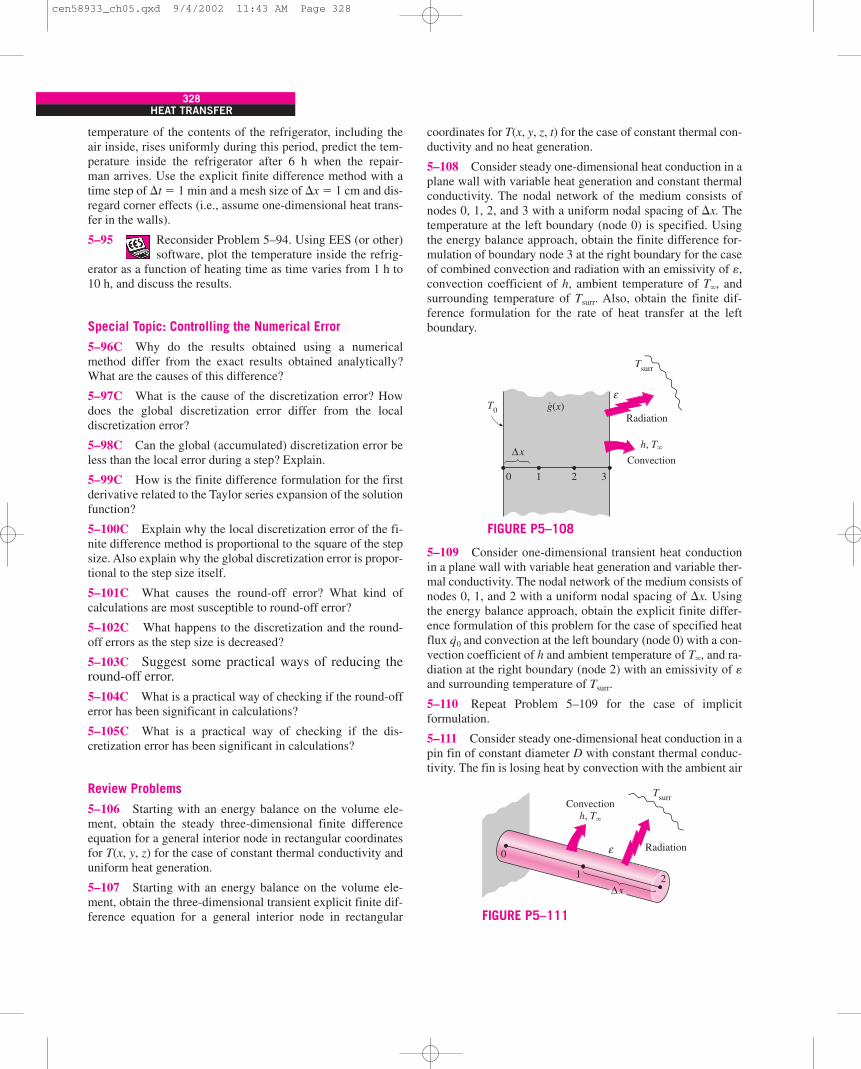
328HEAT TRANSFER

temperature of the contents of the refrigerator, including theair inside, rises uniformly during this period, predict the tem-perature inside the refrigerator after 6 h when the repair-man arrives. Use the explicit finite difference method with atime step of �t � 1 min and a mesh size of �x � 1 cm and dis-regard corner effects (i.e., assume one-dimensional heat trans-fer in the walls).

5–95 Reconsider Problem 5–94. Using EES (or other)software, plot the temperature inside the refrig-

erator as a function of heating time as time varies from 1 h to10 h, and discuss the results.

Special Topic: Controlling the Numerical Error

5–96C Why do the results obtained using a numericalmethod differ from the exact results obtained analytically?What are the causes of this difference?

5–97C What is the cause of the discretization error? Howdoes the global discretization error differ from the localdiscretization error?

5–98C Can the global (accumulated) discretization error beless than the local error during a step? Explain.

5–99C How is the finite difference formulation for the firstderivative related to the Taylor series expansion of the solutionfunction?

5–100C Explain why the local discretization error of the fi-nite difference method is proportional to the square of the stepsize. Also explain why the global discretization error is propor-tional to the step size itself.

5–101C What causes the round-off error? What kind ofcalculations are most susceptible to round-off error?

5–102C What happens to the discretization and the round-off errors as the step size is decreased?

5–103C Suggest some practical ways of reducing theround-off error.

5–104C What is a practical way of checking if the round-offerror has been significant in calculations?

5–105C What is a practical way of checking if the dis-cretization error has been significant in calculations?

Review Problems

5–106 Starting with an energy balance on the volume ele-ment, obtain the steady three-dimensional finite differenceequation for a general interior node in rectangular coordinatesfor T(x, y, z) for the case of constant thermal conductivity anduniform heat generation.

5–107 Starting with an energy balance on the volume ele-ment, obtain the three-dimensional transient explicit finite dif-ference equation for a general interior node in rectangular

coordinates for T(x, y, z, t) for the case of constant thermal con-ductivity and no heat generation.

5–108 Consider steady one-dimensional heat conduction in aplane wall with variable heat generation and constant thermalconductivity. The nodal network of the medium consists ofnodes 0, 1, 2, and 3 with a uniform nodal spacing of �x. Thetemperature at the left boundary (node 0) is specified. Usingthe energy balance approach, obtain the finite difference for-mulation of boundary node 3 at the right boundary for the caseof combined convection and radiation with an emissivity of ,convection coefficient of h, ambient temperature of T�, andsurrounding temperature of Tsurr. Also, obtain the finite dif-ference formulation for the rate of heat transfer at the leftboundary.

5–109 Consider one-dimensional transient heat conductionin a plane wall with variable heat generation and variable ther-mal conductivity. The nodal network of the medium consists ofnodes 0, 1, and 2 with a uniform nodal spacing of �x. Usingthe energy balance approach, obtain the explicit finite differ-ence formulation of this problem for the case of specified heatflux q·0 and convection at the left boundary (node 0) with a con-vection coefficient of h and ambient temperature of T�, and ra-diation at the right boundary (node 2) with an emissivity of and surrounding temperature of Tsurr.

5–110 Repeat Problem 5–109 for the case of implicitformulation.

5–111 Consider steady one-dimensional heat conduction in apin fin of constant diameter D with constant thermal conduc-tivity. The fin is losing heat by convection with the ambient air

∆x

Radiation

Convection

h, T�

0 1 2

ε

3

g(x)·

Tsurr

T0

FIGURE P5–108

0

1

∆x

Radiation

h, T�

ε

Convection

2

Tsurr

FIGURE P5–111

cen58933_ch05.qxd 9/4/2002 11:43 AM Page 328

CHAPTER 5329

at T� (in °C) with a convection coefficient of h, and by radia-tion to the surrounding surfaces at an average temperature ofTsurr (in K). The nodal network of the fin consists of nodes 0 (atthe base), 1 (in the middle), and 2 (at the fin tip) with a uniformnodal spacing of �x. Using the energy balance approach, ob-tain the finite difference formulation of this problem for thecase of a specified temperature at the fin base and convectionand radiation heat transfer at the fin tip.

5–112 Starting with an energy balance on the volume ele-ment, obtain the two-dimensional transient explicit finite dif-ference equation for a general interior node in rectangularcoordinates for T(x, y, t) for the case of constant thermal con-ductivity and uniform heat generation.

5–113 Starting with an energy balance on a disk volume ele-ment, derive the one-dimensional transient implicit finite dif-ference equation for a general interior node for T(z, t) in acylinder whose side surface is subjected to convection with aconvection coefficient of h and an ambient temperature of T�

for the case of constant thermal conductivity with uniform heatgeneration.

5–114E The roof of a house consists of a 5-in.-thick concreteslab (k � 0.81 Btu/h · ft · °F and � � 7.4 � 10�6 ft2/s) that is45 ft wide and 55 ft long. One evening at 6 PM, the slab is ob-served to be at a uniform temperature of 70°F. The ambient airtemperature is predicted to be at about 50°F from 6 PM to10 PM, 42°F from 10 PM to 2 AM, and 38°F from 2 AM to 6 AM,while the night sky temperature is expected to be about 445 Rfor the entire night. The convection heat transfer coefficients atthe inner and outer surfaces of the roof can be taken to behi � 0.9 and ho � 2.1 Btu/h · ft2 · °F, respectively. The houseand the interior surfaces of the walls and the floor are main-tained at a constant temperature of 70°F during the night, andthe emissivity of both surfaces of the concrete roof is 0.9.Considering both radiation and convection heat transfers andusing the explicit finite difference method with a mesh size of

�x � 1 in. and a time step of �t � 5 min, determine the tem-peratures of the inner and outer surfaces of the roof at 6 AM.Also, determine the average rate of heat transfer through theroof during that night.

5–115 Solar radiation incident on a large body of clean water(k � 0.61 W/m · °C and � � 0.15 � 10�6 m2/s) such as a lake,a river, or a pond is mostly absorbed by water, and the amountof absorption varies with depth. For solar radiation incident ata 45° angle on a 1-m-deep large pond whose bottom surface isblack (zero reflectivity), for example, 2.8 percent of the solarenergy is reflected back to the atmosphere, 37.9 percent is ab-sorbed by the bottom surface, and the remaining 59.3 percentis absorbed by the water body. If the pond is considered to befour layers of equal thickness (0.25 m in this case), it can beshown that 47.3 percent of the incident solar energy is ab-sorbed by the top layer, 6.1 percent by the upper mid layer, 3.6percent by the lower mid layer, and 2.4 percent by the bottomlayer [for more information see Çengel and Özisik, Solar En-ergy, 33, no. 6 (1984), pp. 581–591]. The radiation absorbed bythe water can be treated conveniently as heat generation in theheat transfer analysis of the pond.

Consider a large 1-m-deep pond that is initially at a uniformtemperature of 15°C throughout. Solar energy is incident onthe pond surface at 45° at an average rate of 500 W/m2 for a pe-riod of 4 h. Assuming no convection currents in the water andusing the explicit finite difference method with a mesh size of�x � 0.25 m and a time step of �t � 15 min, determine thetemperature distribution in the pond under the most favorableconditions (i.e., no heat losses from the top or bottom surfacesof the pond). The solar energy absorbed by the bottom surfaceof the pond can be treated as a heat flux to the water at that sur-face in this case.

ε

ε

Concreteroof

Radiation

Radiation

Convection

Convection

hi, Ti

Ti

ho, To

Tsky

FIGURE P5–114E

0

x

Solar pond

Solarradiation

45°

Top layer

Upper mid layer

Lower mid layer

Bottom layer Black

1

2

3

4

qs, W/m2·

Sun

FIGURE P5–115

cen58933_ch05.qxd 9/4/2002 11:43 AM Page 329

330HEAT TRANSFER

5–116 Reconsider Problem 5–115. The absorption of solarradiation in that case can be expressed more accurately as afourth-degree polynomial as

g·(x) �q·s(0.859 � 3.415x � 6.704x2 � 6.339x3 � 2.278x4), W/m3

where q·s is the solar flux incident on the surface of the pond inW/m2 and x is the distance from the free surface of the pondin m. Solve Problem 5–115 using this relation for the absorp-tion of solar radiation.

5–117 A hot surface at 120°C is to be cooled by attaching8 cm long, 0.8 cm in diameter aluminum pin fins (k � 237W/m · °C and � � 97.1 � 10�6 m2/s) to it with a center-to-center distance of 1.6 cm. The temperature of the surroundingmedium is 15°C, and the heat transfer coefficient on the sur-faces is 35 W/m2 · °C. Initially, the fins are at a uniform tem-perature of 30°C, and at time t � 0, the temperature of the hotsurface is raised to 120°C. Assuming one-dimensional heatconduction along the fin and taking the nodal spacing to be�x � 2 cm and a time step to be �t � 0.5 s, determine thenodal temperatures after 5 min by using the explicit finite dif-ference method. Also, determine how long it will take forsteady conditions to be reached.

5–118E Consider a large plane wall of thickness L � 0.3 ftand thermal conductivity k � 1.2 Btu/h · ft · °F in space. Thewall is covered with a material having an emissivity of � 0.80 and a solar absorptivity of �s � 0.45. The inner sur-face of the wall is maintained at 520 R at all times, while theouter surface is exposed to solar radiation that is incident at arate of q·s � 300 Btu/h · ft2. The outer surface is also losing heat

by radiation to deep space at 0 R. Using a uniform nodal spac-ing of �x � 0.1 ft, (a) obtain the finite difference formulationfor steady one-dimensional heat conduction and (b) determinethe nodal temperatures by solving those equations.

Answers: (b) 522 R, 525 R, 527 R

5–119 Frozen food items can be defrosted by simply leavingthem on the counter, but it takes too long. The process canbe speeded up considerably for flat items such as steaks byplacing them on a large piece of highly conducting metal,called the defrosting plate, which serves as a fin. The increasedsurface area enhances heat transfer and thus reduces the de-frosting time.

Consider two 1.5-cm-thick frozen steaks at �18°C that re-semble a 15-cm-diameter circular object when placed next toeach other. The steaks are now placed on a 1-cm-thick black-anodized circular aluminum defrosting plate (k � 237W/m · °C, � � 97.1 � 10�6 m2/s, and � 0.90) whose outerdiameter is 30 cm. The properties of the frozen steaks are � 970 kg/m3, Cp � 1.55 kJ/kg · °C, k � 1.40 W/m · °C,� � 0.93 � 10�6 m2/s, and � 0.95, and the heat of fusion ishif � 187 kJ/kg. The steaks can be considered to be defrostedwhen their average temperature is 0°C and all of the ice in thesteaks is melted. Initially, the defrosting plate is at the roomtemperature of 20°C, and the wooden countertop it is placed oncan be treated as insulation. Also, the surrounding surfaces canbe taken to be at the same temperature as the ambient air, andthe convection heat transfer coefficient for all exposed surfacescan be taken to be 12 W/m2 · °C. Heat transfer from the lateralsurfaces of the steaks and the defrosting plate can be neglected.Assuming one-dimensional heat conduction in both the steaksand the defrosting plate and using the explicit finite differencemethod, determine how long it will take to defrost the steaks.Use four nodes with a nodal spacing of �x � 0.5 cm for thesteaks, and three nodes with a nodal spacing of �r � 3.75 cmfor the exposed portion of the defrosting plate. Also, use a timestep of �t � 5 s. Hint: First, determine the total amount of heattransfer needed to defrost the steaks, and then determine howlong it will take to transfer that much heat.

0

2

h, T�

T0 Convection

4

1

3

2 cm

FIGURE P5–117

∆x

Radiation

0 1 2ε

3

qs·

sα

Tsurr

T0

FIGURE P5–118E

20°C

Heattransfer

6 5

1234

Symmetry line

Defrostingplate

Steaks

FIGURE P5–119

cen58933_ch05.qxd 9/4/2002 11:43 AM Page 330

CHAPTER 5331

5–120 Repeat Problem 5–119 for a copper defrosting plateusing a time step of �t � 3 s.

Design and Essay Problems

5–121 Write a two-page essay on the finite element method,and explain why it is used in most commercial engineeringsoftware packages. Also explain how it compares to the finitedifference method.

5–122 Numerous professional software packages are avail-able in the market for performing heat transfer analysis, andthey are widely advertised in professional magazines such asthe Mechanical Engineering magazine published by the Amer-ican Society of Mechanical Engineers (ASME). Your companydecides to purchase such a software package and asks youto prepare a report on the available packages, their costs, ca-pabilities, ease of use, and compatibility with the availablehardware, and other software as well as the reputation of thesoftware company, their history, financial health, customersupport, training, and future prospects, among other things.After a preliminary investigation, select the top three packagesand prepare a full report on them.

5–123 Design a defrosting plate to speed up defrosting of flatfood items such as frozen steaks and packaged vegetables andevaluate its performance using the finite difference method(see Prob. 5–119). Compare your design to the defrosting

plates currently available on the market. The plate must per-form well, and it must be suitable for purchase and use as ahousehold utensil, durable, easy to clean, easy to manufacture,and affordable. The frozen food is expected to be at an initialtemperature of �18°C at the beginning of the thawing processand 0°C at the end with all the ice melted. Specify the material,shape, size, and thickness of the proposed plate. Justify yourrecommendations by calculations. Take the ambient and sur-rounding surface temperatures to be 20°C and the convectionheat transfer coefficient to be 15 W/m2 · °C in your analysis.For a typical case, determine the defrosting time with andwithout the plate.

5–124 Design a fire-resistant safety box whose outer dimen-sions are 0.5 m � 0.5 m � 0.5 m that will protect its com-bustible contents from fire which may last up to 2 h. Assumethe box will be exposed to an environment at an average tem-perature of 700°C with a combined heat transfer coefficient of70 W/m2 · °C and the temperature inside the box must be be-low 150°C at the end of 2 h. The cavity of the box must be aslarge as possible while meeting the design constraints, and theinsulation material selected must withstand the high tempera-tures to which it will be exposed. Cost, durability, and strengthare also important considerations in the selection of insulationmaterials.

cen58933_ch05.qxd 9/4/2002 11:43 AM Page 331

cen58933_ch05.qxd 9/4/2002 11:43 AM Page 332

NUMERICAL METHODS IN HEAT CONDUCTION Skntu.ac.ir/DorsaPax/userfiles/file/Mechanical/... ·...

Documents

Transcript of NUMERICAL METHODS IN HEAT CONDUCTION Skntu.ac.ir/DorsaPax/userfiles/file/Mechanical/... ·...