E. Dieterich G. Sorescu G. Eigenberger

FEDERAL REPUBLIC OF GERMANY

Numerical methods for the simulation of

chemical engineering processes

Fundamental aspects and the current state of the art in simu­lating the dynamic and steady-state behavior of chemical engi­neering processes are discussed. The discretization of the spatial derivatives in the equations of change leads to a system of differ­ential algebraic equations (DAE), consisting of ordinary differen­tial equations in the time domain, and algebraic equations. The present paper discusses the necessary steps to solve the DAE, and mentions proven standard software for these steps as well as for the solution of the differential algebraic equations as a whole.

1. Introduction

Chemical engineering research and development is based on the analysis and on the purposeful utiliza-tion of the relevant physical-chemical interactions. In this context, mathematical modeIing of these inter-actions and their numerical simulation keep gaining an increasing importance; they enable to concentrate experimental investigations on well-defined aspects, to discover complex relationships through the inter-play between experiment and numerical simulation, and to commercially exploit these.

From Chemie-Ingenieur-Technik 64, No. 2, pp. 136-147 (1992), with permission. Dipl.-Ing. Erwin Dieterich, Dr.-log. Gheorge Sorescu, and Professor Dr.-log. Gerhart Eigenberger are associated with the Institut ftir Chemische Verfahrenstechnik, Universitat Stuttgart, BobIinger Str. 72, D70199 Stuttgart 1.

0020.631813414-04551$5.00 0 1994, American Institute ofChemi-cal Engineers.

Whereas mathematical analysis of experiments is distinguished by a long and proven tradition in chemical engineering, detailed mathematical model-ing and numerical simulation are techniques within the framework of chemical engineering training that are covered with an intensity greatly varying from one place to another. In addition, CUITent develop-ment of methods and procedures used in computer simulation is so rapid that it increasingly becomes more difficult to follow its growth.

In this paper, on the one hand, important fun-damentals of numerical simulation are sketched, standard methods are explained, and a few sources that are suitable for their study in depth are men-tioned. On the other hand, developments are dis-cussed which have an effect on the application of numerical simulation, and which may become sig-nificant for its future use. In contrast to the com-puter scientist, or the (numerical) mathematician, the engineer usually considers numerical simulation as a tool with whose details he wants to become acquainted only up to a point which is necessary

INTERNATIONAL CHEMICAL ENGINEERING Vol. 34, No. 4 October 1994 455

brought to you by COREView metadata, citation and similar papers at core.ac.uk

provided by Online Publikationen der Universität Stuttgart

for its practical application. This paper is based on that premise. However, it is apparent that, with the help of standard numerical tools, only standard prob-lems of computer simulation may be solved, and that each foray into new territory forces consideration of the whole spectrum of numerical methods available. The present paper also contains comments on this problem.

Physically meaningful mathematical models of chemical engineering equipment and plants are based on the equations for conservation of mass, mo-mentum, and energy. For most applications, so far they have been limited to the use of one or two spatial coordinates; often, only the steady state is treated. The latter limitation, however, is removed in this treatment, partly because consideration of dy-namics becomes increasingly important for the un-derstanding of chemical engineering equipment and processes, and, partly, because inclusion of dynam-ics often requires only small extra effort as compared with the calculation of the steady state, and some-times it even assures a better convergence of the so-lution than a purely steady-state calculation. Above all, however, dynamic simulation may be carried out by using a highly standardized scheme, the so-termed method of lines.

1.1. Introductory ezample

As an introductory example, the model of an isothermal tubular reactor is considered that can be characterized by the mass balance on the concentra-tion C of a key component for a controlling reaction. Using the spatially one-dimensional diffusion con-vection equation, the mass balance is as follows:

8c lPc 8c B at = D 8z2 - v 8z + S(c, z, t) (1)

with the initial condition

c(t = O,z) = cO(z)

and the boundary conditions

Bcl D-8 = v(c(t, z = 0) - c*) Z %=0

Bcl _ 0 Bz %=L -

(2)

(3)

(4)

The source term S(c, z, t) describes the rate of re-action which depends on the concentration c usually in a nonlinear fashion, and that may also explicitly depend on position and time. The capacity factor B in Equation (1) is equal to unity. Nevertheless, it is

convenient to explicitly carry B in the subsequent manipulations.

Equation (1) is a nonlinear partial differential equation (PDE) of the convection-diffusion type, which is widely used for the description of chem-ical engineering equipment, characterized by one-dimensional flow.

The customary technique used for its numerical so-lution is the method of lines. This technique is based on discretization of the spatial derivative

DlPc _v 8c 8z2 8z

(5)

e.g., by a simple equidistant difference approximation at point I, using step size Az:

8c I ~ CHI - cl-I 8z I 2Az

(6)

lPcl 8 (~) 8z2 I 8z

CHI - 2Cl + Cl-I = Az2 (7)

This way, within the solution interval, the PDE is transformed into a system of NZ ordinary differen-tial equations. The equation at the point oflineariza-tion 1 becomes

where D v

0= Az2 + 2Az

-2D {3=-Az2

D v 'Y = AZ2 - 2Az

(9)

(10)

(11)

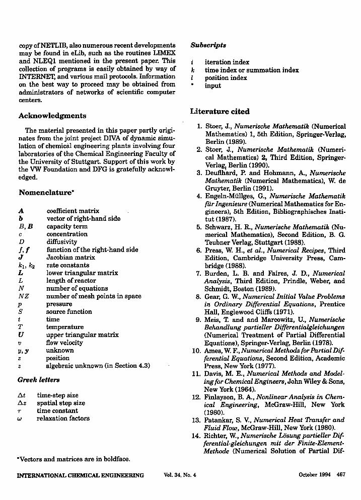
In view of coupling between Cl, Cl-I, cl+I, the system of equations must be solved simultaneously. Inspec-tion of the solution plane t above z (cf. Figure 1) offers an explanation for the term method of lines. After dis-cretization with respect to spatial derivatives, each of the ordinary differential equations (8) obtained is solved along a z = constant line.

Equation (8), written in vectorial notation, is as follows:

dy B dt =~, z, t) (12)

where B is the capacity matrix; y is the solution vec-tor; andfon the right-hand side is the function vector

456 October 1994 Vol. 34, No. 4 INTERNATIONAL CHEMICAL ENGINEERING

t c..1 C1 C1.1

tt+1

t= 0

1-1 1+1 z

I 0 I 0 I 0 I Robmaktor

Fig. 1. Spatial discretization and integration with respect to time of Equation (1) by the method of lines.

1 1

B= 1

1 1

Cl h C2 h

y = C, ;f= 11 (13)

CNZ-I INZ-I

CNZ INz

A solution of the system (12) of first-order, nonlinear differential equations can be carried out by first dis-cretizing the time coordinate t, using the index k and the time step Llt:

•• ••• ••• ••• ••• ••• ••• •• a)

DD ODD

ODD DD

b) c)

Next, the nonlinear right-hand side fmust be lin-earized. Thislinearization can be carried out, e.g., by expanding f about the old solution yk. The relation-ship is as follows:

(15)

where &f/ {)y is the matrix of partial derivatives of the right-hand side I with respect to all solutions V, the so-termed Jacobian matrix, at the known time k.

The solution at the new time k + I, therefore, re-quires solution of the linear system of equations

(16)

where both the matrix of coefficients A and the vector b on the right-hand side can be determined with the help of model constants and the solutions at the last stepyk.

The amount of computation required for the so-lution of the system of Equations (16) depends on the structure of the matrix A, i.e., on the number of elements in A that are different from zero, and on the pattern of the nonzero elements. With ease, it can be shown that the pattern is usually deter-mined by the structure of the Jacobian matrix &f/ {)y. In the introductory example used, the Jacobian ma-trix is tridiagonal (cf. Figure 2a) because, according to Equation (8), at point oflinearization I, the concen-trations Cl-I. Cz, and CHI appear in the mass balance. If the model of the tubular reactor under considera-tion not only consists of a PDE of one concentration but if also, e.g., equations for other concentrations as well as for temperature, pressure, and density are required, then, in the vector y [Equation (13)], a sub-vector appears instead of Cl, consisting of the vari-ables at point I, mentioned above. The function 11 in the function vector f is replaced by a subvector of the appropriate spatially discretized right-hand side at point 1. Then, 8fi/ {)Y, is the Jacobian submatrix at point oflinearization 1, and, therefore, &f/{)Y and also A obtain a block tridiagonalstructure (ef. Figure 2b) .

Fig. 2. Customary structures of the Jacobian ma-trix J = 8(/ ()y or the solution matrix A [Equation (16)]. a) tridiagonal structure of the introductory example; b) block tridiagonal structure when con-sidering several state variables; c) convection-diffusion system with recycle.

INTERNATIONAL CHEMICAL ENGINEERING Vot. 34, No. 4 October 1994 457

If, instead of simple flow through a reactor, a tubu-lar reactor with recycle were considered, then, the first element I = 1 (input) would be coupled with the last element I = NZ (output). In the pattern of the Jacobian matrix and of the A matrix, the additional coupling block at position (1, NZ) is shown in Figure 2c. In this way, the peculiarities of spatial coupling are built into the matrix A of the linear system of Equation (16) for each piece of equipment and each process in an unambiguous way.

Also, the capacity matrix B introduced by Equa-tions (1), (12), and (13) plays an important role for an efficient and routine numerical treatment of the model equations. In the introductory example, B cor-responds to the unit matrix; often, B is a diagonal matrix. Situations exist, however, where time deriva-tives of several state variables appear in the same balance equation, e.g., an enthalpy balance for com-pressible fluids leads to a sum of the time derivatives of temperature (aT/at) and total pressure (Op/at) that can be considered in B without any additional transformation. From Equation (16), it is apparent that the system of equations may also be solved if B is not regular, i.e., if the system contains rows of zeros. An important example is the calculation of th~ steady-state solution. Here, all time deriva-tives disappear and B becomes the zero matrix. Un-der these conditions, Equation (16) describes an iter-ative scheme for the steady-state solution yk by the Newton-Raphson method (see Section 3), where k de-notes the iteration step. In any event, the solution of the linear system of Equations (16) must be repeated until yk+l sufficiently well agrees with yk.

In addition, during the course of model formula-tion, often nonlinear coupling relationships appear between state variables that do not contail). time derivatives. Typical examples are equations of state or phase equilibrium relationships; quasisteady-state balance equations also belong here. This means that Equation (12) often does not represent a system of ordinary differential equations but it contains dif-ferential equations and nonlinear equations which are coupled with one another by f and, occasionally, also by B. It has become customary to refer to thi8 situation as that of differential algebra equations <DAE).

Quite in general, a physically based mathemati~ model of a chemical engineering process, after dis-cretization of the, spatial derivatives, leads to a DAE such as represented by Equation (12). DAE may be solved with the help of so-termed DA solvers (er. Sec-tion 4). The introductory example shows a particu-larly simple procedure for this solution. In all situa-tions, a linear system of equations that has a struc-

ture as the one shown by Equation (16) results, and that must be iteratively solved.

In the following section, the individual steps: 1. discretization with respect to the space coordi-

nate; 2. discretization with respect to the time coordi-

nate; 3. solution of the nonlinear system of equations;

and 4. solution of the linear system of equations are

discussed in greater detail and in the opposite order.

2. Solution of linear systems of equations

2.1. Direct solution procedure (LU decomposition)

Formally, the solution of the linear system of equa-tions

A3=b (17)

is carried out by finding the inverses (A)-I:

y=A-1b (18)

This procedure, however, usually is not carried out explicitly because of the large amount of calculations involved. Rather, A is decomposed by suitable trans-formation into the product of a lower triangular ma-trix L (er. Figure 3a) and an upper triangular matrix U (er. Figure 3b) [1, 3-6]:

A=LU (19)

With the knowledge of L and U, the solution ofEqua-tion (16) or, equivalently, of

LUy=b (20)

can be reduced to two simple single steps: using the

a) b) Rg. 3. Decomposition of A according to Equation (19) into a) an upper triangular matrix U; and b) a lower triangular ma-trix L.

458 October 1994 Vol. 34, No. 4 INTERNATIONAL CBEMICAL ENGINEERING

substitution Uy = x, first, the system of equations

(21)

is solved by forward substitution for the determina-tion of x. If x is known, the solution vector y follows by substitution from

Uy=X (22)

The decisive advantage of this procedure is that the sohition' may be easily found for any right-hand side b after carrying out the decomposition of A into LU. This advantage may be exploited in various situ-ations in numerical simulation of chemical engineer-ing processes.

In the LU decomposition, attention must be paid to pivoting. The pivoting is necessary in order to avoid division by zero in the transformation of A, or round-ing off significant digits through small differences of large numbers. Pivoting is frequently facilitated by appropriate scaling of the state variables y, e.g., on the interval 1-1, 1]; er. [2,4,6].

Numerous reliable standard routines are available for the purpose of LU decomposition (er. Section 2.3) so that the process engineer only very seldom needs to do any explicit programming. In general, it holds valid that the structure of A decisively influences the ease of solution of the linear system of equations. Therefore, it is logical to group the model equations in such a way that A possesses a standard domi-nance. This standard dominance fucludes, in partic-ular, tridiagonal and block tridiagonal dominances, both of which are shown in Figure 2. The tridiagonal and block tridiagonal patterns have the advantage that they keep their structure in the process of LU decomposition, if no pivoting is required.

Sometimes, it happens that model building does not lead to any of the standard patterns shown in Figure 2, and, instead, the nonzero elements are very irregularly distributed over the matrix. This distri-bution especially occurs for coupling of various pieces of equipment or processes, i.e., for plant simulation. Here, A has only a few nonzero elements, and it is referred to as a sparse matrix. For such sparse ma-trices, special so-termed sparse solvers exist, which limit the storage place and the necessary calculations to the nonzero elements of the matrix.

2.2. Iterative solution techniques

The solution techniques discussed up to this point are so-termed direct methods. For dense matrices, these techniques permit the solution of systems consisting of a few thousand equations, and, for dis-

tinctly diagonally dominant matrices, even the solu-tions of many more. Because the amount of calcula-tion increases faster than in direct proportion to the number of equations N, an upper limit of N exists beyond which a direct solution is not justified either from the point of view of the amount of calculation to be carried out or from the point of view of the in-creasing extent of round-off errors. The upper limit depends on the so-termed conditioning of the matrix and on the computing accuracy available. This limit may be easily reached and also exceeded, particularly in the simulation of model equations of two or three spatial dimensions.

One way out of this difficulty is by using iterative solution techniques. However, whereas direct meth-ods always lead to the solution, for a nonexcessive number of equations N and a regular matrix A, con-vergence with the classical iterative methods is only assured for diagonally dominant systems. Modem iterative methods are capable of creating diagonal dominance by using suitable transformations [3, 6].

According to the simplest version of an iterative solution technique, the so-termed Jacobian method, the nth equation of the system of equations is solved for the nth unknown in each iteration step, indepen-dently of the ~ther equations. Then, for Equation (17), e.g.,

Hl_ 1 ( ~ i) Y n - - bn - ~ an,k Yk ann k=l,k~n

(23)

where an,k are the elements of A. Here, i is the itera-tion index. This indicates that ~ways the unknowns from the previous iteration are substituted into the right-hand side.

Ifthe unknowns converge, iterative methods have the advantage to be insensitive to rounding off errors, an4, for sparse matrices, iterations require only little storage capacity.

2.8. S~/fware for the solution of linear systems of equations

I

. For! a direct solution of systems of equations with block tridiagonal or tridiagonal structure, the library routines of LINPACK [18] or the IMSL library [19] can be recommended. These routines are just as the rest of the numerical software recommended here, written in standard FORTRAN 77, and they are based on LU decomposition and partial pivoting.

For the direct solution of systems of sparse matri-ces, a generally accepted solution technique is not established. A very frequently used program is the Harwell routine MA30, or its variant MA28 by Duff and Reid [20, 21], which is easier to use and whose

INTERNATIONAL CHEMICAL ENGINEERING Vol. 34, No. 4 October 1994 459

strength lies in the application of information ob-tained in the first LU decomposition for subsequent solutions of problems with a similar pivotal struc-ture. In recent years, various new algorithms have been published [22-24] that, however, mostly do not reach the speed of MA 30 for repeated solutions of problems of identical structure such as in the simu-lation of chemical engineering processes [25].

Iterative methods for the solution of linear systems of equations do not yet reach the reliability provided by direct solution. In practice, tests must be carried out in every individual situation whether or not a method converges for the particular problem at hand. On the basis of the developments in recent years, e.g., [26], however, significant progress may be expected in the field using special strategies for improvement in convergence and of combinations of direct and itera-tive methods.

Basically, standard methods such as those de-scribed in this section always result in a slower solu-tion of a system of equations than an algorithm that was optimized for a particular matrix structure; how-ever, the amount of work required for such nonstan-dard methods is only warranted for very time-critical applications.

Each numerical simulation is ultimately based on repeated solutions of linear systems of equations. From the users point of view, therefore, the develop-ers of general solution packages for nonlinear equa-tions or DA systems should uncouple their programs from the solution oflinear systems of equations, and provide general interfaces. Only, then, the incorpora-tion of specific linear equation solvers will be possible without unreasonable expense.

3. Solution of nonlinear systems of equations

The iterative solution of a nonlinear equation in one unknown

O=/(y)

by Newton's method, using the iteration index i

HI _ i I(yi) Y - Y - I'(yi)

(24)

(25)

is generally known. Generalization of this iteration procedure to systems of equations is the so-termed Newton-Raphson method which can be formally writ-ten as a fixed-point iteration:

Here, J~) is the Jacobian matrix that was already introduced in connection with Equation (15)

8ft 8ft 8ft ayl 81J2 .. ' ayn

8h 8h 8h J~) = ayl 81/2 ... 8Yn (27)

81n 81n 81n 8YI 81/2 ... 8Yn

In practice, instead of a matrix inversion, the linear system of equations

equivalent to Equation (26), with

yi+l = yi + l:lyi

(28)

(29)

is iteratively solved until the residual vector l:lyi be-comes less than a prescribed value [1, 3, 5]. In the in-troductory example, only the first step in the N ewton-Raphson iteration was used in Equations (15) and (16), where the initial value was the solution vector at the old time step tk.

The reason for frequent use of either the direct or the modified Newton-Raphson method is its simple algorithm and its quadratic, i.e., faster than linear convergence. On the other hand, this convergence is only assured if sufficiently good initial values are used. Hence, the solution of large nonlinear systems of equations may run into great difficulties because if several solutions exist the algorithm does not neces-sarily converge to the desired or to a physically mean-ingful solution. In conjunction with the solution of a DAE, these convergence problems, however, are less severe because the previous time step provides a good starting value for the iteration, while the size of the change l:ly can be arbitrarily decreased by reduction of the size of the time step.

Exceptions to this rule may be expected in two sit-uations: at the start of the program if inconsistent starting values are used (ef. Section 4), or for func-tions with a local or a global minimum in the vicinity of the solution. This type of problem can be easily understood for one unknown. The equation 0 = y2 has a (double) zero at y = O. At the same time, the global minimum of the function is at the same place. Thus, I' (y = 0) = O. Here, the iteration procedure (25) leads to a division by zero.

Additional difficulties may arise if the function f is not defined everywhere, because the Newton-Raphson method does not always monotonously con-verge but often oscillates about the solution. If the

460 October 1994 Vol. 34, No. 4 INTERNATIONAL CHEMICAL ENGINEERING

function is not defined in the vicinity of a zero, then, an evaluation might be required in an unde-fined region. AB a simple example, the reaction rate-expression r = cO.5 may be used. A reasonable idea is to assign the value of zero to the reaction rate for neg-ative concentrations. However, this assignment may prevent convergence of the Newton-Raphson proce-dure because here the derivative of the function f in the vicinity of the solution is no more continuous. A logical way out of this difficulty is to continue the function without interruption into the undefined re-gion, e.g., by lettingr(c < 0) = -lclo.5 •

In the process of determination of the Jacobian, the first question to answer is whether or not to use an analytical solution or an approximate numerical calculation. AB a rule, an analytical evaluation of the derivatives leads to more accurate results, and mostly also in a shorter time. However, analytical differentiation of complicated functions requires te-dious work which may be subject to errors. Examples for this are implicit relationships for the calculation of multicomponent equilibria, and complicated reac-tion rate-expressions. Therefore, in many library pro-grams, the option exists of numerically calculating the Jacobian matrix:

8fi ....... h(Yj + dYj) - fi(Yj) 8yj ....... dYj

(30)

In this process, care must be taken to avoid obliter-ation of significant digits by suitable scaling and by choice of step size dYi' By taking advantage of that the Jacobian matrix usually is sparse, the number of function calls for the calculation off(y + l:!.y) can be significantly reduced by altering before each function call several components of f. Thus, in our introduc-tory example for the complete calculation of the tridi-agonal Jacobian, four function evaluations are suffi-cient, independently of the number of discretization points.

Because, in the last few years, powerful programs for symbolic calculations have become available, e.g., MAPLE [35] or MACSYMA [36], today, analytical derivatives can be determined in a simple and ac-curate manner. The result is available in FORTRAN code, and may directly be transferred to the equation solver.

In the iteration according to Equation (26), primar-ily, two cost factors appear:

(1) solution of the linear system of equations; and (2) calculation of the Jacobian matrix J. Efficient procedures for the solution of linear sys-

tems of equations were discussed in the previous sec-tion. The simplest strategy for decreasing the amount of work required for the calculation of the Jacobian

matrix consists of keeping the Jacobian matrix con-stant throughout several iteration steps, whereby the order and the radius of convergence are diminished. On the other hand, the determination of the Jacobian matrix and the LU decomposition becomes unneces-sary. To what extent this possibility can be exploited to advantage depends on the particular situation at hand.

Another possible way consists of not repeatedly cal-culating the entire Jacobian matrix but to improve in each iteration step the matrix determined at the out-set. Procedures along these lines are mostly based on the method developed by Broyden [28]. These procedures have the disadvantage that they create additional nonzero elements in the matrix. Several authors [29, 30] tackled the problem of Broyden up-dates while maintaining the matrix density almost unchanged.

A convenient possibility for influencing the rate and the radius of convergence in the Newtonian pro-cess is the relaxation expressed by

(31)

In this process, a step with w > 1 is referred to as overrelaxation, whereas a step with w < 1 is termed underrelaxation. Overrelaxation is used to increase the convergence rate. Of practical significance is pri-marily the underrelaxation whereby the convergence radius can be significantly increased [3, 14].

8.1. Standard software for the solution of nonlinear systems of equations

Newtonian and quasi-Newtonian methods are available for the calculation of zeros of nonlinear sys-tems of equations in all the large standard mathe-maticallibraries, e.g., such as IMSL or Harwell. The program NLEQl ofDeufthard [31] was found by the authors to be particularly useful in the solution of critical problems such as in the calculation of simul-taneous chemical equilibria, and, also, in the process ofinitia1ization ofDA systems; see Section 4.2. This program has a very effective control of the relaxation parameter w. Recent reviews of and comparison be-tween various solution methods ofnonlinear systems of equations from the point of view of the chemical en-gineer were presented by Sacham [32] and Sun [33].

4. Integration of differential equations

During the course of model building, generally, sys-tems of partial differential equations, ordinary differ-ential equations of first and higher order, and alga-

INTERNATIONAL CBEMICAL ENGINEERING Vot. 34, No. 4 October 1994 461

braic equations are generated. With the help of the method oflines, the partial differential equations can be reduced to a system of ordinary differential equa-tions. Transformation of ordinary differential equa-tions of a higher order into a system of differential equations of first order is carried out by simple sub-stitution.

First, the integration of an ordinary differential equation of first order with a nonlinear right-hand side f(y, t) is considered:

y' = dy = f(y, t) dt (32)

The simplest possibility consists of approximating the differential quotient dy / dt by a difference quo-tient, e.g.,

dy yk+l _ y" dt = ~t = f(y, t) (33)

The next question is how to use a suitable ap-proximation for the function f(y, t) in the interval (t", t" + ~t). A flexible way of accomplishing this is provided by the general Euler method (cf. Figure 4).

"+1 " Y ~; Y = (1-a)f(y", t")+af(yk+l, t"+~t) (34)

Letting a = 0, i.e., f(y, t) :::::: f(y", t"), the so-termed explicit Euler method is obtained, permitting solu-tion for y"+l:

(35)

In contrast to this method, the so-termed implicit Eu-ler method with a = 1, i.e., f(yk+l, t" + ~t), in gen-eral, results in a nonlinear relationship that must be solved by iterations, using the methods described in the previous section

"+1 " Y ~~ Y = f(yk+l, t" + ~t) (36)

Explicit Euler method a .. 0

Trapezoidal rule a .. 0.5

Implicit Euler method a .. 1

,,+. Fig. 4. Integration of Equation (32) using the general Euler method [Equation (34)].

Both of these methods reach a first-order accuracy. For a = 1/2, from Equation (34), the so-termed trape-zoidal rule follows, which is also implicit since fk+l is required, but this rule reaches a second-order ac-curacy.

In this context, nth-order accuracy indicates that the discretization error in the solution of the differ-~ntial equation is proportional to ~tn. By using a higher-order method, the discretization error can be reduced to a greater extent by decreasing ~t.

Using a central difference approximation of the time derivative, the following explicit procedure is obtained, which is also of the order of two:

An analysis, however, shows that an unstable par-asitic solution is brought in by the discretization pro-cess. This analysis leads, independently of the choice bf ~t, after several steps to oscillations of increasing amplitude about the true solution so that, as a result, Equation (37) turns out to be useless [7].

A necessary condition for a solution algorithm is, therefore, first of all, a stable approximation of the time derivative. This condition is satisfied for the gen-eral Euler method. Nevertheless, even here undesir-able oscillations may occur if a < 1, and the time step is greater than a certain value. The undesirable os-cillations are shown in Figure 5 on the example of the stable linear differential equation .

dy T-=-y dt (38)

1.0 r-----.---,.--.--...... --.--.--....... -,---,

y

0.5

y(t)

-0.0 \ , .... .... \ I \ /0-0

\ / / \/

-0.5 0.0 2.0 4.0 8.0 8.0

Fig. 5. Numerical solution of Equation (38) with ~t = 1.57 using the implicit (a = 1) and the explicit (a = 0) Euler method.

462 Octoller 199t VoL.a4, No. 4 INTERNATIONAL CHEMICAL ENGINEERING

with the solution

yet) = yO exp (-tiT) (39)

With the help of Equations (35) and (36), the devel-opment of the numerical solution for large time steps can be easily followed. For the explicit Euler method, the solution starts to oscillate in the example as soon as f::l.t > T, and it exponentially increases as soon as f::l.t > 2T. In contrast, the implicit Euler method monotonously approaches the exact solution, even for arbitrary large time steps f::l.t.

This result may be generalized in a remarkable way: all purely explicit integration methods for the solution of stable differential equations become un-stable above a limiting value of the time-step size ~tcritJ where f::l.tcrit is of the order of magnitude of the smallest time constant T or the smallest recipro-cal eigenvalue of the linearized differential equation. In contrast, implicit solution metho-ds permit time steps that are also significantly greater than T. This result is of great importance for the solution of sys-tems of differential equations (cf. Section 4.1). On the other hand, no reason exists to prefer the implicit to the explicit method in the solution of individual dif-ferential equations of first order, since, in order to obtain an accurate solution, the time step must be chosen to be smaller than the value of the time con-stant anyhow. The amount of calculations involved in the explicit methods is, by the very nature, signifi-cantly less compared to the implicit method. For this reason, in the past, mainly explicit solution meth-ods were used for ordinary differential equations. The m.ost popular examples are the classical fourth-order Runge-Kutta method, the Adams-Moulton, and the Adams-Bashford methods [8].

For an efficient use of an integration method, automatic time-step control must be used. Control assures, in addition to providing stability (in the explicit method) and convergence (in the implicit m.ethod), also a control of the errors, and minimiza-tion of the computing time required for the solution of a problem. In most situations, control of the time-step size is based on an error estimation, e.g., by a comparison of results obtained with different step sizes f::l.t.

4.1. Integration of a system of ordinary differential equations

In the integration of a system of ordinary differen-tial equations,

(40)

with a regular matrix B, application of one of the explicit methods described above may run into sig-

nificant difficulties. These difficulties are illustrated on a short example. The concentration evolution in an isothermal batch reactor of constant volume is to be calculated for a simple situation of two reactions in series:

(41)

The time dependence of concentration is described by the following first-order differential equations:

dCA d1 = -k1cA (42)

dcB d1 =k1cA -k2cB (43)

dcc d1 =k2cB (44)

Analytical solution of this system is as follows:

CA = CAO exp (-kIt) (45)

CAO CC = k k (-k2 exp (-kIt) + kl exp (-k2t» + CAO

2 - I (47)

where CAO is the concentration of the eductA at time t = o. Ifreaction (2) is much faster than reaction (1), then, the term exp (-k2t) rapidly vanishes and the dynamic behavior of the system is only determined by exp (-kIt). Figure 6 shows the concentration evo-lution for values of the rate constant kl = 1 and k2 = 106• Note should be made that the solution is almost exclusively determined by the slow dynamics with TI = 1/kl = 1 after a very short initial time pe-riod. Nevertheless, when using the explicit method of integration, for the reasons explained above, the time-step size of the order of magnitude of the least time constant must be chosen, i.e., T2 = 1/k2 = 106

(I), in order to keep the solution stable. Such a system is referred to as stiff. As a measure of stiffness, gen-erally, the ratio of the least to the greatest real part of the eigenvalues of the system of differential equa-tions can be used [5]. Integration of a stiff system of the form of Equation (40) with an explicit method is not very effective: the number of the integration steps which are only necessary for the sake of stability and not for the sake of accuracy becomes so great that the integration can only be conveniently carried out with implicit methods.

For nonlinear differential equations, the eigen-values follow from the equations linearized about the respective solution. Therefore, the stiffness can strongly change during the course of the solution pro-cess. The least eigenvalue of a system of equations

INTERNATIONAL CHEMICAL ENGINEERING Vol. 34, No. 4 October 1994 463

c c

0.5 5.0.-06

0.0 L-.o--'"--'--'-...L... ........ .......;i::::.._ 0.0.+00 1IoG.I ....... --'-........ ...L... ........................ -.I Fig. 6. a) Concentration versus time curves for a consecutive reaction [Equation (41)] for kl = 1, k2 = 106; b) short time dynamics of the consecutive reaction.

0.0 2.5 5.0 0.0.+00 5.0.-06

a.) b)

arising from spatial discretization of a PDE also de-pends on the size chosen for the spatial step. For these and the other reasons mentioned in Section 4.2, it is advisable not to use the explicit integration methods in connection with the method of lines.

The semiimplicit Euler method [37] used in the in-troductory example

BY -y =~k)+ _ (yk+l_yk) k+l k fJ( I ll.t ay 7"

(48)

can be obtained from the implicit Euler method, Equation (36), by linearizing the term f f+k about the old time point tk, and leads to the formally explicit in-tegration procedure

(B-at :IJ y'+1

= (B -at :1,.) ,.. + Mlr) (49)

without losing the stability properties of the implicit Euler method [17]. Therefore, it is also suitable for stiff systems. This example forms the basis ofLIMEX [47], an efficient standard procedure for the solution of DAEs; er. Section 4.4.

4.2. Integration of differentiol algebra systems

In general, the model of chemical engineering equipment consists of differential equations that de-scribe its dynamic behavior, and of algebraic cou-pling, DAE. The model may also be expressed in the

1.0.-05

form of Equation (40), where the matrixB is singular, i.e., it contains empty rows and/or columns. Typical examples for linear and nonlinear coupling relation-ships are represented by the boundary conditions of PDEs, phase equilibria, equations of state, and PDEs assumed to be in quasi-steady state. The DAE may be solved as a stiff system with the help of implicit integration methods [38], provided its index (er. next section) is less or equal to unity. Algebraic relation-ships can be visualized as differential equations with an infinitely short oscillation time; DAEs are, there-fore, infinitely stiff systems of differential equations.

For the numerical solution of a DAE, the initial conditions must be specified. However, the number of the initial conditions that can be freely chosen, i.e., the degrees of freedom of the DAE may be less than the number of variables whose time derivatives are contained in the system. This issue will be discussed in greater detail in the next section. In any event, for the start of integration, the additional (not freely selectable) variables must be determined in an ini-tialization step in such a way that they satisfy the DAE at the initial point of time. For this purpose, a transformation of the DAE which is described in the next section should be used.

4.3. Index problems

In most situations, a DAE may be solved without any difficulty with the help of implicit or semiim-plicit integration methods. In some situations, how-ever, a particular structural property ofDAEs, the s~ termed index, has a detrimental effect. Various ways exist of defining the index, among which the most widely used is to define a differential index [40, 41].

464 October 1994 Vol. 34, No. 4 INTERNATIONAL CHEMICAL ENGINEERING

According to its definition, the differential index kd of a DAE is the number of derivatives necessary in order to transform the DA system into a system of ordinary differential equations (ODE). A DAE with an index kd :5 1 may be integrated with the help of the above-described methods for stiff systems of dif-ferential equations. The integration of systems with kd ~ 2, however, may lead to severe problems so that standard methods often do not work.

For a demonstration of these deficiencies, the fol-lowing simple example is considered:

Y~=YI+2Y2+2z

Y~=YI-Y2-Z

(50)

(51)

(52)

The integration is characterized by the peculiar-ity that YI and Y2 are algebraically coupled through Equation (52). Evidently, therefore, only one of these equations can be freely specified as an initial condi-tion, whereas the initial value ofthe other, along with the variable z, must be determined in an initializa-tion step. However, this initialization is not immedi-ately possible because no explicit relationship exists for the calculation of z. For the determination of z, Equation (52) can first be differentiated:

(53)

After substitution of(50) and (51) into (53), the fol-lowing algebraic relationship which was hidden in the original system is obtained:

(54)

Now, z can be calculated. After differentiation of Equation (54) and substitution of Equations (50) and (51), the following differential equation for z is ob-tained:

z' = -3(YI + Y2 +z) (55)

Since two differentiations were necessary for the transformation of the original DAEs (50) to (52) into the system of ordinary differential equations (50), (51), and (55), the differential index of the original system is two.

For a general handling of index problems for kd ~ 2, Bachmann et al. [45,46] suggested developing the hidden algebraic coupling from the original DAE by differentiation and substitution, and to solve the al-gebraic equations along with the required number of differential equations. In the above-mentioned exam-ple, the substitute system consists of Equations (52) and (54), in addition to one of the three differential

---------------------------------j

equations, namely, Equations (50), (51), and (55), and the system has a differential index of kd = 1.

The example shows that, due to the structure of the DAE, all three variables YI, Y2, and z play an equal role, and that to which of these an initial condition (degree of freedom) should be assigned is a matter of arbitrary choice. In practice, which of these variables will be used as the initial condition depends on the nature of the physical problem.

Transformation of the original DAE by differentia-tion and substitution may require a great deal of cal-culations for complicated systems. Under such condi-tions, it is convenient to substitute a new (algebraic) unknown for the derivative of one of the variables to be eliminated, with the result that the derivatives of the algebraic coupling conditions supply the ad-ditional equations necessary for the solution of the problem. In the above-mentioned example, the sub-stitution of y~ = Z2 in Equation (53) results in the equivalent DAE with the index kd = 1:

y~ = YI + 2Y2 + 2z

0=YI-Y2-Z- Z2

0= YI +Y2

y~ = -Z2

(56)

(57)

(58)

(59)

Although the system now has an additional new variable, the amount of work necessary for transfor-mation was significantly reduced.

For dynamic models of chemical engineering pro-cesses, index problems may always arise whenever the state variables are coupled with one another by equations of state, phase equilibrium relationships, or special transport expressions. In this connection, a problem may arise already in the formulation of the fundamental partial differential equations [42]. The way to proceed here, i.e., before spatial discretization has taken place, is subject to ongoing research.

4.4. Standard software for DABs

Using the integration routines contained in the large program libraries of numerical mathematics, e.g., IMSL, NAG, and Harwell, simple problems can be solved without any difficulties and in a short time. However, in general, to use programs in which more recent results of mathematical research are imple-mented is more effective, since, particularly in the field of numerical integration of DAEs, significant progress has been made in the eighties. The following methods were found to be very effective:

(1) backward differential formula (BDF) methods; (2) extrapolation methods; and (3) implicit Runge-Kutta methods.

INTERNATIONAL CHEMICAL ENGINEERING Vol. 34, No. 4 October 1994 465

The programs DASSL [43] and LSODElLSODI [44], based on the BDF method, found the most widespread use. The extrapolation codes developed by Deuflhard [3], e.g., EULSIM and LIMEX [47], were found to be extremely effective in our applications, and were found to be equally valuable compared to DASSL in the solution of problems of practical rel-evance. In recent years, a strong interest developed in the implicit Runge-Kutta method [48-50]. The re-spective codes, e.g., RADAU5 [50], did not yet reach the level of the above-named programs, but, in the near future, further progress may be expected.

All the above-mentioned programs contain auto-matic error and step-size monitoring; in addition, LIMEX is in a position to detect problems with an index kd>2, and to automatically reject these. In general, these routines solve a problem in compa-rable lengths of time, and, in each individual situ-ation, it must be established which method is the most suitable. If, in a system, a large number of switching processes exist, which manifest themselves in discontinuities of the right-hand side~, t) of the mathematical models, then, one-step methods such as the extrapolation or the Runge-Kutta methods are to be preferred because, with multistep methods such as BDF, a restart must be performed with low order.

The simultaneous methods of dynamic plant simu-lation such as DIVA [51] or SPEEDUP [52] are based on DAE solvers of high performance, where the mod-els of individual plant parts are discretized in space, and combined to one single large DAE (40), which is solved with the methods described above.

5. Integration of partial differential equations

As has been shown in the introductory example, systems of PDEs can be transformed into a DAE by discretization with respect to the position coor-dinates. Whereas, for the solution of a DAE, the above-described comprehensive and tested method of solution exists, permitting the solution with a pre-determined accuracy, the technique of spatial dis-cretization is not equally well developed. In particu-lar, the chemical engineer himself must usually also carry out spatial discretization when using commer-cial simulation software, unless he or she prefers pre-manufactured process modules with a limited scope. As a rule, in these modules, the errors arising from spatial discretization are not considered or limited.

A large number of methods is available for the dis-cretization of spatial derivatives. The best known for chemical engineering applications are the finite dif-ference methods and the finite element methods. In

the one-dimensional situation, both yield either iden-tical or: similar systems of equations. Due to its sim-plicity of handling, the difference method is preferred in the one-dimensional situation and sometimes also in the two-dimensional case. As an example, the dif-ference approximation carried out in Equations (5) to (7) of the introductory example may be mentioned.

The problems arising in the discretization of spa-tial derivatives and their convenient handling will not be discussed in this paper, but it will be presented in a separate pUblication. At this point, only refer-ence is made to some introductory and comprehen-sive monographs [9, 10]. Introductory chapters deal-ing with the treatment of PDEs may also be found in some standard texts on numerical mathematics [5, 6]. The methods used for the solution of chemical engineering problems are discussed in [11, 12]. An introduction to the so-termed finite volume method may be found in [13] and to the finite element method in [14 to 16].

6. Sources of information and codes

This survey of numerical methods for the simula-tion of dynamic and stationary behavior of chemical engineering processes was meant to review the pro-cedures that were· established and tested in recent years. More detailed information may be found in the references indicated. It was pointed out that, for the solution of linear systems of equations, the solution ofnonlinear systems of equations, and the solution of DAEs, proven standard codes are available so that in-dividual programming of these steps may be limited to a few special situations.

The standard codes are usually contained as FOR-TRAN 77 subprograms, on the one hand, in the large commercially operated numerical libraries requiring licensing fees, such as IMSL, Harwell, or NAG. On the other hand, in recent years, a number of in-teresting codes have become available without fees as public domain software, i.e., these subprograms may be freely copied and used. An example of this is the LAPACK collection for the solution of linear systems of equations, along with the BLAS routines simultaneously developed for the purpose of funda-mental vector and matrix operations. (BLAS = Ba-sic Linear Algebra Subroutines.) These routines are available, and can be copied without charge at most university computer centers throughout the world. ,Additional general or specialized codes are centrally collected at various locations. The best known server of programs of numerical math is NETLm. The largest similar collection in Germany is the eLib of the Konrad-Zuse-Zentrum in Berlin. In addition to a

466 October 1994 Vol. 34, No. 4 INTERNATIONAL CHEMICAL ENGINEERING

copy ofNETLm, also numerous recent developments may be found in eLib, such as the routines LIMEX and NLEQl mentioned in the present paper. This collection of programs is easily obtained by way of INTERNET, and various mail protocols. Information on the best way to proceed may be obtained from administrators of networks of scientific computer centers.

Acknowledgments

The material presented in this paper partly origi-nates from the joint project DNA of dynamic simu-lation of chemicitl engineering plants involving four laboratories of the Chemical Engineering Faculty of the University of Stuttgart. Support of this work by the VW Foundation and DFG is gratefully acknowl-edged.

Nomenclature*

A b B,B c D f,r J kt, k2 L L N NZ p S t T U v y,y z z

coefficient matrix vector of right-hand side capacity term concentration diffusivity function of the right-hand side Jacobian matrix rate constants lower triangular matrix length of reactor number of equations number of mesh points in space pressure source function time temperature upper triangular matrix flow velocity unknown position algebraic unknown (in Section 4.3)

Greek letters

l:l.t time-step size l:l.z spatial step size T time constant w relaxation factors

·Vectors and matrices are in boldface.

Subscripts

i k I •

iteration index time index or summation index position index input

Literature cited

1. Stoer, J., Numerische Mathematik (Numerical Mathematics) 1, 5th Edition, Springer-Verlag, Berlin (1989).

2. Stoer, J., Numerische Mathematik (Numeri-cal Mathematics) 2, Third Edition, Springer-Verlag, Berlin (1990).

3. Deuflhard, P. and Hohmann, A., Numerische Mathematik (Numerical Mathematics), W. de Gruyter, Berlin (1991).

4. Engeln-Miillges, G., Numerische Mathematik fUr Ingenieure (Numerical Mathematics for En-gineers), 5th Edition, Bibliographisches Insti-tut (1987).

5. Schwarz, H. R., Numerische Mathematik (Nu-merical Mathematics), Second Edition, B. G. Teubner Verlag, Stuttgart (1988).

6. Press, W. H., et al., Numerical Recipes, Third Edition, Cambridge University Press, Cam-bridge (1988).

7. Burden, L. B. and Faires, J. D., Numerical Analysis, Third Edition, Prindle, Weber, and Schmidt, Boston (1989).

8. Gear, G. W., Numerical Initial Value Problems in Ordinary Differential Equations, Prentice Hall, Englewood Cliffs (1971).

9. Meis, T. and and Marcowitz, u., Numerische Behandlung partieller Differentialgleichungen (Numerical Treatment of Partial Differential Equations), Springer-Verlag, Berlin (1978).

10. Ames, W. F., Numerical Methods for Partial Dif-ferential Equations, Second Edition, Academic Press, New York (1977).

11. Davis, M. E., Numerical Methods and Model­ing for Chemical Engineers, John WHey & Sons, New York (1964).

12. Finlayson, B. A., Nonlinear Analysis in Chem­ical Engineering, McGraw-Hill, New York (1980).

13. Patankar, S. v., Numerical Heat Transfer and Fluid Flow, McGraw-Hill, New York (1980).

14. Richter, w., Numerische Losung partieller Dif­ferential-gleichungen mit der Finite-Element­Methode (Numerical Solution of Partial Dif-

INTERNATIONAL CHEMICAL ENGINEERING Vol. 34, No. 4 October 1994 467

ferentia1 Equations with the Finite Element Method), F. Vieweg & Sohn, Braunschweig (1986).

15. Villadsen, J. V. and Michelsen, M. L., Solu­tion of Differential Equation Models by Polyno­mial Approximation, Prentice-Hall, Englewood Cliffs (1980).

16. Schwarz, H. R., Methode der finiten Elemente (The Finite Elements Method), Second Edition, B. G. Teubner Verlag, Stuttgart (1984).

17. Deuflhard, P., Numerik von Anfangswertmeth­oden fUr gewohnliche Differentialgleichungen (Numerical Initial Value Methods for Ordinary Differential Equations), FU Berlin, TR 89-2 (1989).

18. Dongarra, J. J., et al., UNPACK User's Guide, SIAM, Philadelphia (1979).

19. IMSL, User's Manual, IMSL Mathematics Li-brary, Houston (1989).

20. Duff, I. S. and Reid, J. K, ACM 7Tans. Math. Software 5, pp. 18-35 (1979).

21. Duff, I. S., Erisman, A. M., and Reid, J. K,Direct Methods for Sparse Matrices, Clarendon Press, Oxford (1987).

22. Stadtherr, M. A. and Wood, E. S., Comput. Chem. Eng. 8, pp. 9-33 (1984).

23. Gilbert, J. and Peierls, T., SIAM J. Sci. Stat. Comp. 9, pp. 862-874 (1988).

24. Osterby, O. and Zlatev, Z., Direct Methods for Sparse Matrices Daimi PB-123, Computer Sci-ence Department, Aarhus University (1980).

25. Ng. E., A Comparison of Some Methods for Solv-ing Sparse Nonsymmetric Linear Systems, Oak Ridge National Laboratory, unpublished draft (1991).

26. Saadi, Y. and Schultz, M. H., SIAM J. Sci. Stat. Comput. 7, pp. 856--870 (1986).

27. Crowe, C. M. and Nishio, M., AIChE J. 21, pp. 3--12 (1975).

28. Broyden, C. G., Math. Camp. 19, pp. 577--593 (1965).

29. Schubert, L. K, Math. Comp. 25, pp. 27--39 (1970).

30. BogIe, I. D. L. and Perkins, J. D., Camp. Chem. Eng. 12, pp. 791--812 (1988).

31. Deuflhard, P., Newton Techniques for Highly Nonlinear Problems-Theory, Algorithms, Codes, Academic Press, New York (in print).

32. Shacham, M., Camp. Chem. Eng. 9, pp. 103--124 (1985).

33. Sun, E. T. and Stadtherr, M. A., Comp. Chem. Eng. 12, pp. 1129--1145 (1988).

34. Stoer, J., in Computational Mathematical Pro­gramming, Klaus Schittkowski, Ed., NATO ASI Series, Springer Verlag, Berlin (1985).

35. Char, B. W., et al., MAPLE Reference Manual, Watcom Publ., Ltd. (1988).

36. MACSYMA Reference Manual, Symbolics, Inc. (1988).

37. Deuflhard, P., SIAM Rev. 27, pp. 505--535 (1988).

38. Gear, C. W., IEEE Trans. Circuit Theory CT-IB, pp. 89--95 (1971).

39. Pantelides, C. C., SIAM J. Sci. Stat. Comput. 9, pp. 213--231 (1988).

40. Petzold, L. R., SIAM J. Sci. Stat. Comput. 3, pp. 367--384 (1982).

41. Gear, C. W. and Petzold, L. R., SIAM J. Numer. Anal. 21, pp. 716-728 (1984).

42. Hindmarsh, A. C. and Johnson, S. H., Chem. Eng. Sci. 43, pp. 3235-3258 (1988).

43. Brenan, K E., Campbell, S. L., and Pet-zold, L. R., Numerical Solution of Initial-Value Problems in Differential-Algebraic Equations, North-Holland Publ. Co., Amsterdam (1989).

44. Hindmarsh, A. C., ACM-Signum Newsletter 15, pp. 10--27 (1980).

45. Bachmann, R., Mrziglod, T., et al., in DECHEMA-Monogr. 116, VCh, Weinheim (1989).

46. Bachmann, R., MrzigIod, T., et al., Comp. Chem. Eng. 14, pp. 1271-1273 (1990).

47. Deuflhard, P., Hairer, E., and Zugck, J., Numer. Math. 51,51, pp. 501-516 (1987).

48. Brenan, K E. and Petzold, L. R., SIAM J. Nu­mer. Anal. 26, pp. 976-996 (1989).

49. Ascher, U. M. and PetzoId, L. R., SIAM J. Numer. Anal. 28, pp. 1097-1120 (1991).

50. Hairer, E., Lubich, C., and Roche, M., The Nu­merical Solution of Differential-Algebraic Sys­tems by Runge-Kutta Methods, Springer Verlag, Berlin (1989).

51. Kroner, A., et al., Comp. Chem. Eng. 14, pp. 1289--1295 (1990).

52. Perkins, J. D. and Sargent, R. W. H., AIChE Symp. Ser. 214, pp. 1-11 (1982).

468 October 1994 Vol. 34, No. 4 INTERNATIONAL CHEMICAL ENGINEERING