
Hyperbolic PDEs Numerical Methods for PDEs Spring 2007 Jim E. Jones.
Upload
duongquynhCategory
view
234download
1
Numerical Methods for PDEsAn introduction
Marc Kjerland
University of Illinois at Chicago
Marc Kjerland (UIC) Numerical Methods for PDEs January 24, 2011 1 / 39

Numerical Methods for PDEs
Outline
1 Numerical Methods for PDEs
2 Finite Difference method
3 Finite Volume method
4 Spectral methods
5 Finite Element method
6 Other considerations
Marc Kjerland (UIC) Numerical Methods for PDEs January 24, 2011 2 / 39

Numerical Methods for PDEs
Preliminaries
We seek to solve the partial differential equation
Pu = f
where u is an unknown function on a domain Ω ⊆ RN , P is a differentialoperator, and f is a given function on Ω. Typically u also satisfies someinitial and/or boundary conditions. It is seldom possible to find exactsolutions analytically.A numerical method will typically find an approximation to u by making adiscretization of the domain or by seeking solutions in a reduced functionspace.
Marc Kjerland (UIC) Numerical Methods for PDEs January 24, 2011 3 / 39

Finite Difference method
Outline
1 Numerical Methods for PDEs
2 Finite Difference method
3 Finite Volume method
4 Spectral methods
5 Finite Element method
6 Other considerations
Marc Kjerland (UIC) Numerical Methods for PDEs January 24, 2011 4 / 39

Finite Difference method
Finite differences
The basic idea for the finite difference method is to replace derivativeswith finite differences. Consider u = u(x , t) and let h, k > 0. Then wecould use the following approximations:
∂u
∂x≈ u(x + h, t)− u(x , t)
h∂u
∂t≈ u(x , t + k)− u(x , t)
k
Marc Kjerland (UIC) Numerical Methods for PDEs January 24, 2011 5 / 39

Finite Difference method
Domain discretization
Let us define a regular grid of points (xm, tn) = (mh, nk) for some integersm and n. In general these points need not be equally spaced. The finitedifference algorithm will generate approximations to u at each grid point.
Marc Kjerland (UIC) Numerical Methods for PDEs January 24, 2011 6 / 39

Finite Difference method
Notation
We introduce the notation unm = u(xm, tn). Then we can write:
∂
∂xunm ≈
unm+1 − un
m
h∂
∂tunm ≈
un+1m − un
m
k.
These are called forward differences; there are many other possible choices.
Marc Kjerland (UIC) Numerical Methods for PDEs January 24, 2011 7 / 39

Finite Difference method
Example
Consider the one-way wave equation:
ut + aux = 0
with initial conditionu(x , 0) = u0(x).
Here is the forward-time forward-space approximation:
un+1m − un
m
k+ a
unm+1 − un
m
h= 0,
from which we can derive the following explicit scheme:
un+1m = (1 + ak
h )unm − ak
h unm+1.
Marc Kjerland (UIC) Numerical Methods for PDEs January 24, 2011 8 / 39
Finite Difference method
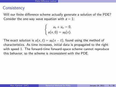
Consistency
Will our finite difference scheme actually generate a solution of the PDE?Consider the one-way wave equation with a = 1:
ut + ux = 0,
u(x , 0) = u0(x).
The exact solution is u(x , t) = u0(x − t), found using the method ofcharacteristics. As time increases, initial data is propagated to the rightwith speed 1. The forward-time forward-space scheme cannot reproducethis behavior, so the scheme is inconsistent with the PDE.
A scheme which is consistent with the one-way wave equation for all a isthe forward-time center-space scheme:
un+1m − un
m
k+ a
unm+1 − un
m−1
2h= 0.
Marc Kjerland (UIC) Numerical Methods for PDEs January 24, 2011 9 / 39
Finite Difference method
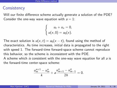
Consistency
Will our finite difference scheme actually generate a solution of the PDE?Consider the one-way wave equation with a = 1:
ut + ux = 0,
u(x , 0) = u0(x).
The exact solution is u(x , t) = u0(x − t), found using the method ofcharacteristics. As time increases, initial data is propagated to the rightwith speed 1. The forward-time forward-space scheme cannot reproducethis behavior, so the scheme is inconsistent with the PDE.A scheme which is consistent with the one-way wave equation for all a isthe forward-time center-space scheme:
un+1m − un
m
k+ a
unm+1 − un
m−1
2h= 0.
Marc Kjerland (UIC) Numerical Methods for PDEs January 24, 2011 9 / 39

Finite Difference method
Stability
A poorly-chosen numerical scheme can sometimes result in uncontrolled(and incorrect) growth of the solution. We say that a finite differencescheme for a first-order equation is stable if there is an integer J such thatfor any positive time T , there is a constant CT such that
‖un‖2h ≤ CT
J∑j=0
‖uj‖2h.
This is typically shown using Von Neumann analyis in Fourier space; thereis often a strong dependence on the relation between h and k .The forward-time center-space scheme for the one-way wave equation isunstable.
Marc Kjerland (UIC) Numerical Methods for PDEs January 24, 2011 10 / 39

Finite Difference method
Implicit schemes
The backward-time center-space scheme is both consistent with theone-way wave equation and unconditionally stable:
un+1m − un
m
k+ a
un+1m+1 − un+1
m−1
2h= 0
This is an implicit scheme, since unknown values appear multiple times inthe equation. Implicit schemes often allow for much larger grid spacingbut require significant additional calculations at each step.
Marc Kjerland (UIC) Numerical Methods for PDEs January 24, 2011 11 / 39

Finite Difference method
Order of accuracy
Consider Poisson’s equation in 2D:
uxx + uyy = f .
The discrete five-point Laplacian approximation is given by:
um+1,n + um−1,n + um,n+1 + um,n−1 − 4um,n = h2fm,n
Marc Kjerland (UIC) Numerical Methods for PDEs January 24, 2011 12 / 39

Finite Difference method
Order of accuracy
The discrete nine-point Laplacian is of higher accuracy: o(h4) vs. o(h2).However, it requires more information at each step:
16 (um+1,n+1 + um+1,n−1 + um−1,n+1 + um−1,n−1)+
+ 23 (um+1,n + um−1,n + um,n+1 + um,n−1)− 10
3 um,n =
= h2
12 (fm+1,n + fm−1,n + fm,n+1 + fm,n−1)
Marc Kjerland (UIC) Numerical Methods for PDEs January 24, 2011 13 / 39

Finite Difference method
Pros and cons of finite difference methods
Advantages:
• Fast
• Easy to code
Disadvantages:
• Hard to generalize in complex geometries
Marc Kjerland (UIC) Numerical Methods for PDEs January 24, 2011 14 / 39

Finite Volume method
Outline
1 Numerical Methods for PDEs
2 Finite Difference method
3 Finite Volume method
4 Spectral methods
5 Finite Element method
6 Other considerations
Marc Kjerland (UIC) Numerical Methods for PDEs January 24, 2011 15 / 39

Finite Volume method
Conservation laws
The finite volume method is used to find numerical solutions toconservation laws. A conservation law is a PDE written generally in theform:
∂tq(x , t) + div F(x , t) = f (x , t),
where q is a conserved quantity (i.e. mass, energy), F is a fluxrepresenting a transport mechanism for q, and f is a forcing term. Thereis an implicit dependence on an unknown u(x , t)
Marc Kjerland (UIC) Numerical Methods for PDEs January 24, 2011 16 / 39

Finite Volume method
Examples of conservation laws
Linear transport equation:∂tu(x , t) + div(vu)(x , t) = 0, t > 0,
u(x , 0) = u0(x).
[q = u(x , t),F = vu(x , t), f = 0]
Stationary diffusion equation:−∆u = f , on Ω = (0, 1)× (0, 1)
u = 0, on δΩ
[q = u(x),F = −∇u(x)]
Marc Kjerland (UIC) Numerical Methods for PDEs January 24, 2011 17 / 39

Finite Volume method
Examples of conservation laws
1D Euler equations:
∂t
ρρuE
+ ∂x
ρuρu2 + p
u(E + p)
= 0.
Marc Kjerland (UIC) Numerical Methods for PDEs January 24, 2011 18 / 39

Finite Volume method
Intro to the Finite Volume method
Let Ω ⊆ Rd be our spatial domain, and let T be a polygonal mesh on Ω.Consider a control volume K ∈ T . Integrating over K , we have by thedivergence theorem:∫
K∂tq(x , t)dx +
∫∂K
F(x , t) · nK (x)dσ =
∫K
f (x , t)dx .
Let NK ⊆ T be the set of neighbors of K . Then∫K∂tq(x , t)dx +
∑L∈NK
∫K∩L
F(x , t) · nK (x)dσ =
∫K
f (x , t)dx .
Marc Kjerland (UIC) Numerical Methods for PDEs January 24, 2011 19 / 39

Finite Volume method
Discretization and approximation
Using an explicit forward-time scheme, we can write∫K
qn+1(x)− qn(x)
kdx +
∑L∈NK
ΦnK ,L =
∫K
f (x , tn)dx ,
where ΦnK ,L is an approximation to the flux from K to L.
Marc Kjerland (UIC) Numerical Methods for PDEs January 24, 2011 20 / 39

Finite Volume method
The numerical flux
In a finite volume scheme, we seek an appropriate time discretization aswell as numerical flux terms F n
K ,L which are
• Conservative, i.e. F nK ,L = −F n
L,K .
• Consistent with the PDE.
Marc Kjerland (UIC) Numerical Methods for PDEs January 24, 2011 21 / 39

Finite Volume method
Pros and cons of finite volume methods
Advantages:
• Robust and cheap for conservation laws
• Can handle complex geometries
Disadvantages:
• High precision difficult (see: Discontinuous Galerkin)
Marc Kjerland (UIC) Numerical Methods for PDEs January 24, 2011 22 / 39

Spectral methods
Outline
1 Numerical Methods for PDEs
2 Finite Difference method
3 Finite Volume method
4 Spectral methods
5 Finite Element method
6 Other considerations
Marc Kjerland (UIC) Numerical Methods for PDEs January 24, 2011 23 / 39
Spectral methods
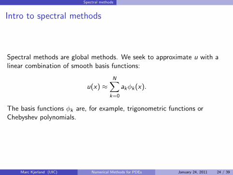
Intro to spectral methods
Spectral methods are global methods. We seek to approximate u with alinear combination of smooth basis functions:
u(x) ≈N∑
k=0
akφk(x).
The basis functions φk are, for example, trigonometric functions orChebyshev polynomials.
Marc Kjerland (UIC) Numerical Methods for PDEs January 24, 2011 24 / 39

Spectral methods
Basis functions
The choice of basis functions should meet three requirements:
1 Approximation∑N
k=0 akφk(x) must converge rapidly.
2 Given ak , it should be easy to determine bk such thatddx
(∑Nk=0 akφk(x)
)=∑N
k=0 bkφk(x).
3 It should be fast to convert between coefficients ak , for k = 0, . . . ,N,and values v(xi ) at some set of nodes xi , for i = 0, . . . ,N.
Marc Kjerland (UIC) Numerical Methods for PDEs January 24, 2011 25 / 39

Spectral methods
Basis functions
Periodic problems: Trigonometric functions satisfy (1) and (2)immediately. Thanks to the FFT (1965), they also satisfy (3).
Non-periodic problems: Legendre and Chebyshev polynomials are thepreferred choice.
Marc Kjerland (UIC) Numerical Methods for PDEs January 24, 2011 26 / 39

Spectral methods
Determining coefficients
To determine the expansion coefficients, we consider the residual R(x , t)when the expansion is substituted in the governing equation. There arethree main techniques:
• Tau. Select ak to satisfy BCs, make the residual orthogonal to asmany basis functions as possible.
• Galerkin. Combine basis functions into a new set in which allfunctions satisfy the BCs, then make residual orthogonal to as manyof the new basis functions as possible.
• Collocation (PS). Select ak to satisfy BCs, make residual zero at asmany spatial points as possible.
Marc Kjerland (UIC) Numerical Methods for PDEs January 24, 2011 27 / 39

Spectral methods
Pros and cons of spectral methods
Advantages:
• Error decays rapidly with N
• Small dissipative and dispersive errors
• Can handle coarse grids
Disadvantages:
• Complex geometries
• Shock handling
Marc Kjerland (UIC) Numerical Methods for PDEs January 24, 2011 28 / 39

Finite Element method
Outline
1 Numerical Methods for PDEs
2 Finite Difference method
3 Finite Volume method
4 Spectral methods
5 Finite Element method
6 Other considerations
Marc Kjerland (UIC) Numerical Methods for PDEs January 24, 2011 29 / 39

Finite Element method
Intro to the finite element method
We seek to solve a PDE of the form
Pu = f
by finding an approximation u ∈ V, for some function space V. We wish tominimize the residual R(x) :
Pu − f = R(x).
Marc Kjerland (UIC) Numerical Methods for PDEs January 24, 2011 30 / 39

Finite Element method
Choosing a basisWe choose V usually to be the set of continuous or C 1 functions which arepiecewise polynomial of degree p.
Let T be a mesh. Then we choose basis functions φk(x) ∈ V withcompact support over grid cells.
So: u(x) =N∑
k=0
akφk(x).
Marc Kjerland (UIC) Numerical Methods for PDEs January 24, 2011 31 / 39

Finite Element method
Weak formulation
Instead of solving the PDE directly, we solve instead an integral or weakformulation: ∫
Ω(Pu − f )vjdx = 0,
where vj are test functions.
• vj = ∂R∂aj
: Least-squares method.
• vj = 1Ωj: Finite Volume method.
• vj = φj : Galerkin’s method.
Marc Kjerland (UIC) Numerical Methods for PDEs January 24, 2011 32 / 39

Finite Element method
Pros and cons of finite element methods
Advantages:
• Can be very accurate
• Handles complex geometries
Disadvantages:
• ???
Marc Kjerland (UIC) Numerical Methods for PDEs January 24, 2011 33 / 39
Other considerations
Outline
1 Numerical Methods for PDEs
2 Finite Difference method
3 Finite Volume method
4 Spectral methods
5 Finite Element method
6 Other considerations
Marc Kjerland (UIC) Numerical Methods for PDEs January 24, 2011 34 / 39

Other considerations
Boundary Conditions
Boundary Conditions!!
Marc Kjerland (UIC) Numerical Methods for PDEs January 24, 2011 35 / 39
Other considerations
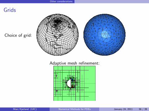
Grids
Choice of grid:
Adaptive mesh refinement:
Marc Kjerland (UIC) Numerical Methods for PDEs January 24, 2011 36 / 39

Other considerations
Computational concerns
• Accuracy vs. speed
• Parallelizability
Marc Kjerland (UIC) Numerical Methods for PDEs January 24, 2011 37 / 39

Other considerations
Other topics of interest
• Continuous Galerkin methods
• Discontinuous Galerkin methods
• Level set methods (Stan Osher, et al)
• Spectral/hp element methods
Marc Kjerland (UIC) Numerical Methods for PDEs January 24, 2011 38 / 39

Other considerations
References
• J. Strikwerda. Finite Difference Schemes and PDEs, (2004).
• R. Eymard , T. Gallou, R. Herbin. Finite Volume Methods, (2006).
• F. Giraldo. Element-based Galerkin Methods, (2010 preprint).
• B. Fornberg. A Practical Guide to Pseudospectral Methods, (1996).
• G. Karniadakis, S. Sherwin. Spectral/hp Element Methods for CFD, (1999).
• C. Johnson. Numerical Solution of PDEs by the Finite Element Method,(2009).
Marc Kjerland (UIC) Numerical Methods for PDEs January 24, 2011 39 / 39


