Numerical Linear Algebra Chap. 1: Basic Concepts from ... · Numerical Linear Algebra Chap. 1:...

Numerical Linear AlgebraChap. 1: Basic Concepts from Linear Algebra

Heinrich [email protected]

Hamburg University of TechnologyInstitute for Numerical Simulation

TUHH Heinrich Voss Chapter 1 2005 1 / 60

http://www.tu-harburg.de/mat/hp/voss/

Basic Ideas from Linear Algebra

Vectors

The vector space Rn is defined by

Rn := {(x1, . . . , xn)T : xj ∈ R, j = 1, . . . , n},

x1x2...

xn

+

y1y2...

yn

=

x1 + y1x2 + y2

...xn + yn

, α

x1x2...

xn

=

αx1αx2

...αxn

and Cn correspondingly.

A subset X ⊂ Rn is a subspace of Rn if it is closed with respect to addition andmultiplication by scalars, i.e.

x , y ∈ X ⇒ x + y ∈ X ,

α ∈ R, x ∈ Rn ⇒ αx ∈ X .



Subspaces

A set of vectors {a1, . . . , am} ⊂ Cn is linearly independent if

m∑j=1

αjaj = 0 ⇒ αj = 0, j = 1, . . . , m.

Otherwise, a nontrivial combination of the aj is zero, and {a1, . . . , am} is saidto be linearly dependent.

Given vectors a1, . . . , am the set of all linear combinations of these vectors is asubspace referred to as the span of a1, . . . , am:

span{a1, . . . , am} =

m∑

j=1

αjaj : αj ∈ C

.



Subspaces ct.

If {a1, . . . , am} is linearly independent and b ∈ span{a1, . . . , am}, then b has aunique representation as linear combination of the aj .

If S1, . . . , Sk are subspace of Cn then their sum

S := S1 + · · ·+ Sk :=

k∑

j=1

aj : aj ∈ Sj , j = 1, . . . , k

is also a subspace of Cn. S is said to be the direct sum if each x ∈ S has aunique representattion x = a1 + · · ·+ ak with aj ∈ Sj . In this case we write

S = S1 ⊕ · · · ⊕ Sk .

The intersection of the subspaces S1, . . . , Sk is also a subspace,

S = S1 ∩ · · · ∩ Sk .



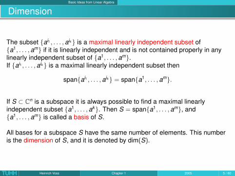
Dimension

The subset {ai1 , . . . , aik } is a maximal linearly independent subset of{a1, . . . , am} if it is linearly independent and is not contained properly in anylinearly independent subset of {a1, . . . , am}.If {ai1 , . . . , aik } is a maximal linearly independent subset then

span{ai1 , . . . , aik } = span{a1, . . . , am}.

If S ⊂ Cn is a subspace it is always possible to find a maximal linearlyindependent subset {a1, . . . , ak}. Then S = span{a1, . . . , am}, and{a1, . . . , am} is called a basis of S.

All bases for a subspace S have the same number of elements. This numberis the dimension of S, and it is denoted by dim(S).



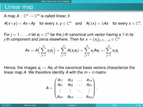
Linear mapA map A : Cn → Cm is called linear, if

A(x+y) = Ax+Ay for every x , y ∈ Cn and A(λx) = λAx for every x ∈ Cn, λ ∈ C.

For j = 1, . . . , n let ej ∈ Cn be the j-th canonical unit vector having a 1 in itsj-th component and zeros elsewhere. Then for x = (xj)j=1,...,n ∈ Cn

Ax = A( n∑

j=1

xjej

)=

n∑j=1

A(xjej) =n∑

j=1

xjAej =:n∑

j=1

xjaj

Hence, the images aj := Aej of the canonical basis vectors characterize thelinear map A. We therefore identify A with the m × n matrix

A =

a11 a12 . . . a1na21 a22 . . . a2n...

.... . .

...am1 a2m . . . amn

.



Matrix-vector product

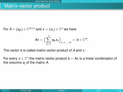
For A = (ajk ) ∈ Cm×n and x = (xk ) ∈ Cn we have

Ax =( n∑

k=1

ajk xk

)j=1,...,m

=: b ∈ Cm.

The vector b is called matrix-vector product of A and x .

For every x ∈ Cn the matrix-vector product b = Ax is a linear combination ofthe columns aj of the matrix A.



Matrix-matrix product

Let A : Cn → Cm and B : Cm → Cp. Then the composition

B ◦ A : Cn → Cp, (B ◦ A)x = B(Ax)

is linear as well, and

BAx = B(Ax) = B( n∑

k=1

ajk xk

)=

m∑j=1

bij

( n∑k=1

ajk xk

)=

n∑k=1

( m∑j=1

bijajk

)xk .

Hence, the composit map of B and A is represented by the matrix-matrixproduct C := BA ∈ Cp×n with elements

cik =m∑

j=1

bijajk , i = 1, . . . , p, k = 1, . . . , n.

Notice that the matrix-matrix product of B and A is only defined if the numberof columns of B equals the number of rows of A.



Range of a matrix

The range of a matrix A, written range(A), is the set of vectors that can beexpressed as Ax for some x . The formula b = Ax leads naturally to thefollowing characterization of range(A).

Theorem 1range(A) is the space spanned by the columns of A.

ProofAx =

∑nj=1 ajxj is a linear combination of the columns aj of A.

Conversely, any vector y in the space spanned by the columns of A can bewritten as a linear combination of the columns, y =

∑nj=1 ajxj . Forming a

vector x out of the coefficients xj , we have y = Ax , and thus y is in the rangeof A.

In view of Theorem 1, the range of a matrix A is also called the column spaceof A.



Nullspace of A

The nullspace of A ∈ Cm×n, written null(A), is the set of vectors x that satisfyAx = 0, where 0 is the 0-vector in Cn.

The entries of each vector x ∈ null(A) give the coefficients of an expansion ofzero as a linear combination of columns of A:

0 = xlal + x2a2 + · · ·+ xnan.

The column rank of a matrix is the dimension of its column space.

Similarly, the row rank of a matrix is the dimension of the space spanned byits rows.

Row rank always equals column rank (among other proofs, this is a corollaryof the singular value decomposition, discussed later), so we refer to thisnumber simply as the rank of a matrix.



Full rankAn m × n matrix of full rank is one that has the maximal possible rank (thelesser of m and n).

This means that a matrix of full rank with m ≥ n must have n linearlyindependent columns. Such a matrix can also be characterized by theproperty that the map it defines is one-to-one.

Theorem 2 A matrix A ∈ Cm×n with m ≥ n has full rank if and only if it mapsno two distinct vectors to the same vector.

Proof If A is of full rank, its columns are linearly independent, so they form abasis for range(A). This means that every b ∈ range(A) has a unique linearexpansion in terms of the columns of A, and therefore, every b ∈ range(A)has a unique linear expansion in terms of the columns of A, and thus, everyb ∈ range(A) has a unique x such that b = Ax .

Conversely, if A is not of full rank, its columns aj are dependent, and there is anontrivial linear combination such that

∑nj=1 cjaj = 0. The nonzero vector c

formed from the coefficients cj satisfies Ac = 0. But then A maps distinctvectors to the same vector since, for any x it holds that Ax = A(x + c).



Inverse matrix

A nonsingular or invertible matrix is a square matrix of full rank.

Note that the m columns of a nonsingular m ×m matrix A form a basis for thewhole space Cm. Therefore, we can uniquely express any vector as a linearcombination of them.

In particular, the canonical unit vector ej , can be expanded:

ej =m∑

i=1

zijaj .

Let Z ∈ Cm×m be the matrix with entries zij , and let zj denote the j th column ofZ . Then it holds ej = Azj , and putting these vectos together

AZ = (e1, . . . , em) =: I

where I ist the m ×m identity. Z is the inverse of A, and is denoted byZ =: A−1.



Gaussian elimination

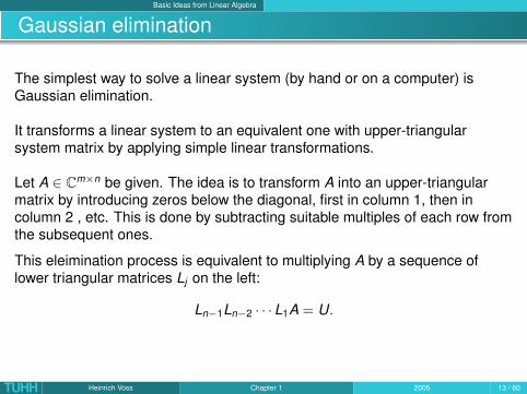
The simplest way to solve a linear system (by hand or on a computer) isGaussian elimination.

It transforms a linear system to an equivalent one with upper-triangularsystem matrix by applying simple linear transformations.

Let A ∈ Cm×n be given. The idea is to transform A into an upper-triangularmatrix by introducing zeros below the diagonal, first in column 1, then incolumn 2 , etc. This is done by subtracting suitable multiples of each row fromthe subsequent ones.

This eleimination process is equivalent to multiplying A by a sequence oflower triangular matrices Lj on the left:

Ln−1Ln−2 · · ·L1A = U.



LU factorization

Setting L := L−11 L−1

2 · · ·L−1n−1 gives A = LU. Thus we obtain an LU

factorization of AA = LU,

where U is upper-triangular, and L is (as a product of lower-triangularmatrices) lower-triangular.

It turns out that L can be chosen such that all diagonal entries are equal to 1.A matrix with this property is called unit lower-triangular.



Example

A =

2 1 3 4−2 1 −1 −24 4 5 11−2 1 −7 −1

The first step of Gaussian elimination looks like this: The first row is added tothe second one, twice the first row is subtracted from the third one, and thefirst row is added to third on. This can be written as

L1A =

1 0 0 01 1 0 0−2 0 1 01 0 0 1

2 1 3 4−2 1 −1 −24 4 5 11−2 1 −7 −1

=

2 1 3 40 2 2 20 2 −1 30 2 −4 3

Next we subtract the second row from the third and the fourth row:

L2L1A =

1 0 0 00 1 0 00 −1 1 00 −1 0 1

2 1 3 40 2 2 20 2 −1 30 2 −4 3

=

2 1 3 40 2 2 20 0 −3 10 0 −6 1



Example ct.

L2L1A =

1 0 0 00 1 0 00 −1 1 00 −1 0 1

2 1 3 40 2 2 20 2 −1 30 2 −4 3

=

2 1 3 40 2 2 20 0 −3 10 0 −6 1

Finally we subtract twice the third row from the fourth row

L3L2L1A =

1 0 0 00 1 0 00 0 1 00 0 −2 1

2 1 3 40 2 2 20 0 −3 10 0 −6 1

=

2 1 3 40 2 2 20 0 −3 10 0 0 −1

To exhibit the full factorization A = LU we need to compute the productL = L−1

1 L−12 L−1

3 .

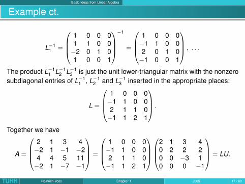
Surprisingly, this turns out to be trivial. The inverse of Lj , j = 1, 2, 3 is just Ljitself, but with each entry below the diagonal negated:



Example ct.

L−11 =

1 0 0 01 1 0 0−2 0 1 01 0 0 1

−1

=

1 0 0 0−1 1 0 02 0 1 0−1 0 0 1

, . . .

The product L−11 L−1

2 L−13 is just the unit lower-triangular matrix with the nonzero

subdiagonal entries of L−11 , L−1

2 and L−13 inserted in the appropriate places:

L =

1 0 0 0−1 1 0 02 1 1 0−1 1 2 1

.

Together we have

A =

2 1 3 4−2 1 −1 −24 4 5 11−2 1 −7 −1

=

1 0 0 0−1 1 0 02 1 1 0−1 1 2 1

2 1 3 40 2 2 20 0 −3 10 0 0 −1

= LU.



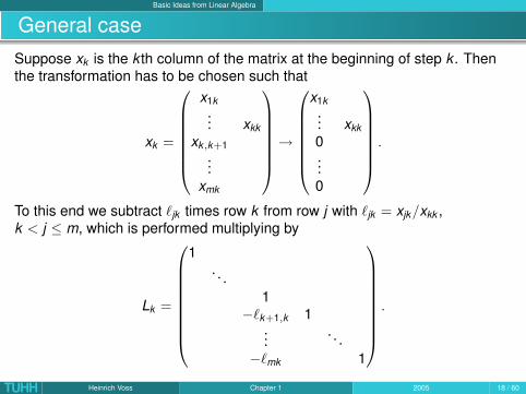
General caseSuppose xk is the k th column of the matrix at the beginning of step k . Thenthe transformation has to be chosen such that

xk =

x1k... xkk

xk,k+1...

xmk

→

x1k... xkk0...0

.

To this end we subtract `jk times row k from row j with `jk = xjk/xkk ,k < j ≤ m, which is performed multiplying by

Lk =

1. . .

1−`k+1,k 1

.... . .

−`mk 1

.



General case ct.

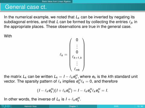
In the numerical example, we noted that Lk can be inverted by negating itssubdiagonal entries, and that L can be formed by collecting the entries `jk inthe appropriate places. These observations are true in the general case.

With

`k =

0...0

`k+1,k...

`mk

the matrix Lk can be written Lk = I − `k eH

k , where ek is the k th standard unitvector. The sparsity pattern of `k implies eH

k `k = 0, and therefore

(I − `k eHk )(I + `k eH

k ) = I − `k eHk `k eH

k = I.

In other words, the inverse of Lk is I + `k eHk .



General case ct.

That L = L−11 · · ·L−1

m can be formed by collecting the entries `jk in theappropriate places is proved by induction.

Assume that

L−11 · · ·L−1

k = I +k∑

j=1

`jeHj .

Then it follws from `jeHj `k+1 = 0 for j = 1, . . . , k

L−11 · · ·L−1

k L−1k+1 = (I +

k∑j=1

`jeHj )(I + `k+1eH

k+1

= I +k+1∑j=1

`jeHj +

k∑j+1

`jeHj `k+1eH

k+1. = I +k+1∑j=1

`jeHj .




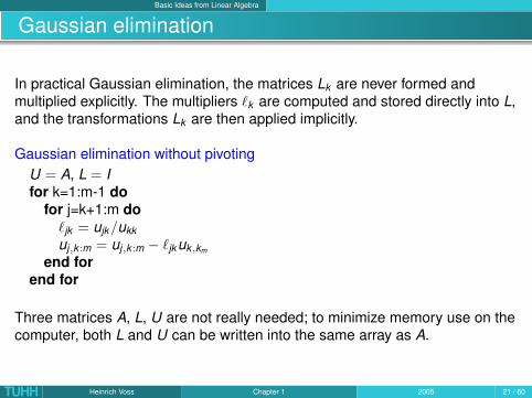
In practical Gaussian elimination, the matrices Lk are never formed andmultiplied explicitly. The multipliers `k are computed and stored directly into L,and the transformations Lk are then applied implicitly.

Gaussian elimination without pivotingU = A, L = Ifor k=1:m-1 do

for j=k+1:m do`jk = ujk/ukkuj,k :m = uj,k :m − `jk uk,km

end forend for

Three matrices A, L, U are not really needed; to minimize memory use on thecomputer, both L and U can be written into the same array as A.



Linear systems

If A is factored into L and U, a system of equations Ax = b is reduced to theform LUx = b.

Thus it can be solved by solving two triangular systems: first Ly = b for theunknown y (forward substitution), then Rx = y for the unknown x (backsubstitution).

This is particularly advantageous, if several linear systems with the samesystem matrix have to be solved.



Failure of Gaussian elimination

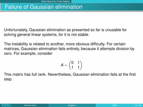
Unfortunately, Gaussian elimination as presented so far is unusable forsolving general linear systems, for it is not stable.

The instability is related to another, more obvious difficulty. For certainmatrices, Gaussian elimination fails entirely, because it attempts division byzero. For example, consider

A =

(0 11 1

)This matrix has full rank. Nevertheless, Gaussian elimination fails at the firststep.



Pivoting

At step k of Gaussian elimination, multiples of row k are subtracted from rowsk + 1, . . . , m of the working matrix X in order to introduce zeros in entry k ofthese rows.In this operation row k , column k , and especially the entry xkk play specialroles. We call xkk the pivot.

From every entry in the submatrix Xk+l:m,k :m is subtracted the product of anumber in row k and a number in column k , divided by xkk

However, there is no reason why the k th row and column must be chosen forthe elimination. For example, we could just as easily introduce zeros incolumn k by adding multiples of some row i with k < i < m to the other rows.

Similarly, we could introduce zeros in column j rather than column k toeliminate in linear system with system matrix the unknown xj from allremaining equations but one.



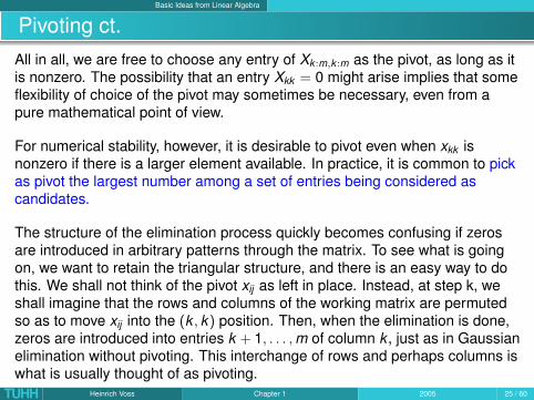
Pivoting ct.All in all, we are free to choose any entry of Xk :m,k :m as the pivot, as long as itis nonzero. The possibility that an entry Xkk = 0 might arise implies that someflexibility of choice of the pivot may sometimes be necessary, even from apure mathematical point of view.

For numerical stability, however, it is desirable to pivot even when xkk isnonzero if there is a larger element available. In practice, it is common to pickas pivot the largest number among a set of entries being considered ascandidates.

The structure of the elimination process quickly becomes confusing if zerosare introduced in arbitrary patterns through the matrix. To see what is goingon, we want to retain the triangular structure, and there is an easy way to dothis. We shall not think of the pivot xij as left in place. Instead, at step k, weshall imagine that the rows and columns of the working matrix are permutedso as to move xij into the (k , k) position. Then, when the elimination is done,zeros are introduced into entries k + 1, . . . , m of column k , just as in Gaussianelimination without pivoting. This interchange of rows and perhaps columns iswhat is usually thought of as pivoting.



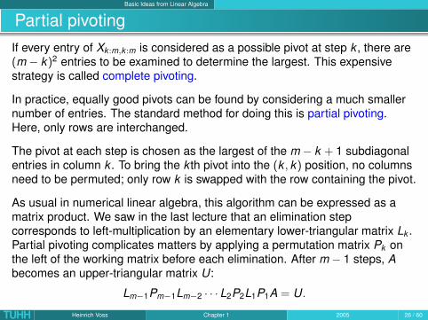
Partial pivotingIf every entry of Xk :m,k :m is considered as a possible pivot at step k , there are(m − k)2 entries to be examined to determine the largest. This expensivestrategy is called complete pivoting.

In practice, equally good pivots can be found by considering a much smallernumber of entries. The standard method for doing this is partial pivoting.Here, only rows are interchanged.

The pivot at each step is chosen as the largest of the m − k + 1 subdiagonalentries in column k . To bring the k th pivot into the (k , k) position, no columnsneed to be permuted; only row k is swapped with the row containing the pivot.

As usual in numerical linear algebra, this algorithm can be expressed as amatrix product. We saw in the last lecture that an elimination stepcorresponds to left-multiplication by an elementary lower-triangular matrix Lk .Partial pivoting complicates matters by applying a permutation matrix Pk onthe left of the working matrix before each elimination. After m − 1 steps, Abecomes an upper-triangular matrix U:

Lm−1Pm−1Lm−2 · · ·L2P2L1P1A = U.



Example

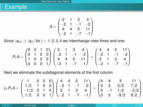
A =

2 1 3 4−2 1 −1 −24 4 5 11−2 1 −7 −1

Since |a31| ≥ |aj1| for j = 1, 2, 3, 4 we interchange rows three and one:

P1A =

0 0 1 00 1 0 01 0 0 00 0 0 1

2 1 3 4−2 1 −1 −24 4 5 11−2 1 −7 −1

=

4 4 5 11−2 1 −1 −22 1 3 4−2 1 −7 −1

Next we eliminate the subdiagonal elements of the first column

L1P1A =

1 0 0 0

1/2 1 0 0−1/2 0 1 01/2 0 0 1

4 4 5 11−2 1 −1 −22 1 3 4−2 1 −7 −1

=

4 4 5 110 3 3/2 7/20 −1 1/2 −3/20 3 −9/2 9/2



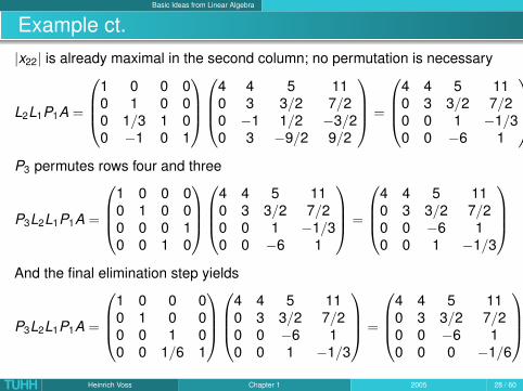
Example ct.|x22| is already maximal in the second column; no permutation is necessary

L2L1P1A =

1 0 0 00 1 0 00 1/3 1 00 −1 0 1

4 4 5 110 3 3/2 7/20 −1 1/2 −3/20 3 −9/2 9/2

=

4 4 5 110 3 3/2 7/20 0 1 −1/30 0 −6 1

P3 permutes rows four and three

P3L2L1P1A =

1 0 0 00 1 0 00 0 0 10 0 1 0

4 4 5 110 3 3/2 7/20 0 1 −1/30 0 −6 1

=

4 4 5 110 3 3/2 7/20 0 −6 10 0 1 −1/3

And the final elimination step yields

P3L2L1P1A =

1 0 0 00 1 0 00 0 1 00 0 1/6 1

4 4 5 110 3 3/2 7/20 0 −6 10 0 1 −1/3

=

4 4 5 110 3 3/2 7/20 0 −6 10 0 0 −1/6



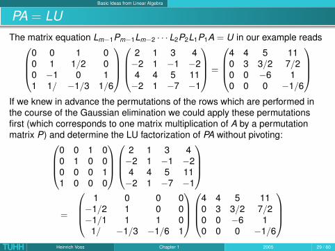
PA = LUThe matrix equation Lm−1Pm−1Lm−2 · · ·L2P2L1P1A = U in our example reads

0 0 1 00 1 1/2 00 −1 0 11 1/ −1/3 1/6

2 1 3 4−2 1 −1 −24 4 5 11−2 1 −7 −1

=

4 4 5 110 3 3/2 7/20 0 −6 10 0 0 −1/6

If we knew in advance the permutations of the rows which are performed inthe course of the Gaussian elimination we could apply these permutationsfirst (which corresponds to one matrix multiplication of A by a permutationmatrix P) and determine the LU factorization of PA without pivoting:

0 0 1 00 1 0 00 0 0 11 0 0 0

2 1 3 4−2 1 −1 −24 4 5 11−2 1 −7 −1

=

1 0 0 0

−1/2 1 0 0−1/1 1 1 0

1/ −1/3 −1/6 1

4 4 5 110 3 3/2 7/20 0 −6 10 0 0 −1/6



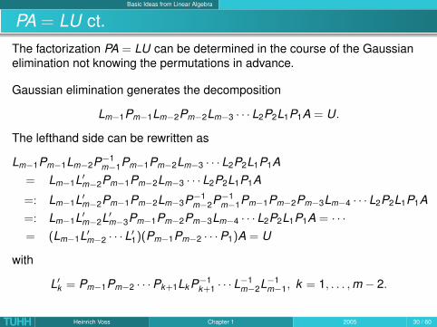
PA = LU ct.The factorization PA = LU can be determined in the course of the Gaussianelimination not knowing the permutations in advance.

Gaussian elimination generates the decomposition

Lm−1Pm−1Lm−2Pm−2Lm−3 · · ·L2P2L1P1A = U.

The lefthand side can be rewritten as

Lm−1Pm−1Lm−2P−1m−1Pm−1Pm−2Lm−3 · · ·L2P2L1P1A

= Lm−1L′m−2Pm−1Pm−2Lm−3 · · ·L2P2L1P1A

=: Lm−1L′m−2Pm−1Pm−2Lm−3P−1m−2P−1

m−1Pm−1Pm−2Pm−3Lm−4 · · ·L2P2L1P1A=: Lm−1L′m−2L′m−3Pm−1Pm−2Pm−3Lm−4 · · ·L2P2L1P1A = · · ·= (Lm−1L′m−2 · · ·L′1)(Pm−1Pm−2 · · ·P1)A = U

with

L′k = Pm−1Pm−2 · · ·Pk+1Lk P−1k+1 · · ·L

−1m−2L−1

m−1, k = 1, . . . , m − 2.



PA = LU ct.

Multiplying Lk by Pk+1 on the left exchanges rows k + 1 and ` for someell > k + 1, and multiplying by P−1

k+1 on the right exchanges columns k + 1 and`. Hence, Pk+1Lk P−1

k+1 has the same structure as Lk , and this structure is keptwhen multiplying with further permutations Pk+2, . . . , Pm−1 and their inverseson the left and right, respectively.

The matrices L′k are unit lower-triangular and easily invertible by negating thesubdiagonal entries, just as in Gaussian elimination without pivoting.

Writing L = (Lm−1L′m−2 · · ·L′1)−1 and P = Pm−1 · · ·P2P1, we have

PA = LU.




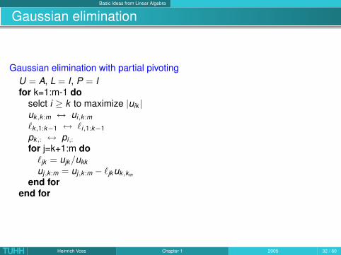
Gaussian elimination with partial pivotingU = A, L = I, P = Ifor k=1:m-1 do

selct i ≥ k to maximize |uik |uk,k :m ↔ ui,k :m`k,1:k−1 ↔ `i,1:k−1pk,: ↔ pi,:for j=k+1:m do

`jk = ujk/ukkuj,k :m = uj,k :m − `jk uk,km

end forend for



Adjoint matrix

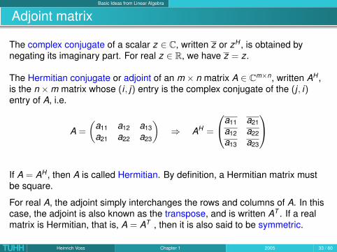
The complex conjugate of a scalar z ∈ C, written z or zH , is obtained bynegating its imaginary part. For real z ∈ R, we have z = z.

The Hermitian conjugate or adjoint of an m × n matrix A ∈ Cm×n, written AH ,is the n ×m matrix whose (i , j) entry is the complex conjugate of the (j , i)entry of A, i.e.

A =

(a11 a12 a13a21 a22 a23

)⇒ AH =

a11 a21a12 a22a13 a23

If A = AH , then A is called Hermitian. By definition, a Hermitian matrix mustbe square.

For real A, the adjoint simply interchanges the rows and columns of A. In thiscase, the adjoint is also known as the transpose, and is written AT . If a realmatrix is Hermitian, that is, A = AT , then it is also said to be symmetric.



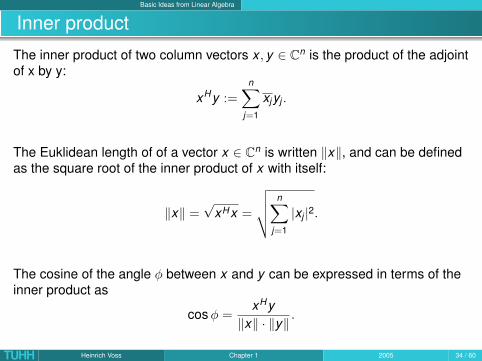
Inner product

The inner product of two column vectors x , y ∈ Cn is the product of the adjointof x by y:

xHy :=n∑

j=1

xjyj .

The Euklidean length of of a vector x ∈ Cn is written ‖x‖, and can be definedas the square root of the inner product of x with itself:

‖x‖ =√

xHx =

√√√√ n∑j=1

|xj |2.

The cosine of the angle φ between x and y can be expressed in terms of theinner product as

cos φ =xHy

‖x‖ · ‖y‖.



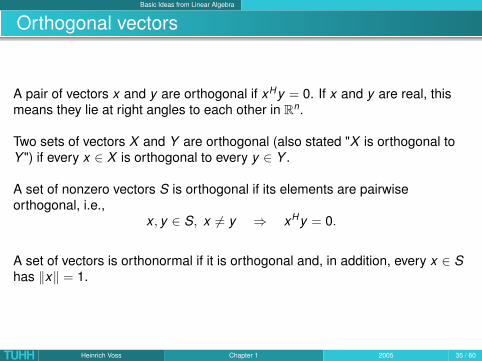
Orthogonal vectors

A pair of vectors x and y are orthogonal if xHy = 0. If x and y are real, thismeans they lie at right angles to each other in Rn.

Two sets of vectors X and Y are orthogonal (also stated "X is orthogonal toY ") if every x ∈ X is orthogonal to every y ∈ Y .

A set of nonzero vectors S is orthogonal if its elements are pairwiseorthogonal, i.e.,

x , y ∈ S, x 6= y ⇒ xHy = 0.

A set of vectors is orthonormal if it is orthogonal and, in addition, every x ∈ Shas ‖x‖ = 1.



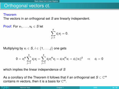
Orthogonal vectors ct.

TheoremThe vectors in an orthogonal set S are linearly independent.

Proof: For v1, . . . , vk ∈ S letk∑

j=1

cjvj = 0.

Multiplying by vi ∈ S, i ∈ {1, . . . , j} one gets

0 = vHi

k∑j=1

cjvj =k∑

j=1

cjvHi vj = civH

i vi = ci‖vi‖2 ⇒ ci = 0

which implies the linear independence of S

As a corollary of the Theorem it follows that if an orthogonal set S ⊂ Cm

contains m vectors, then it is a basis for Cm.



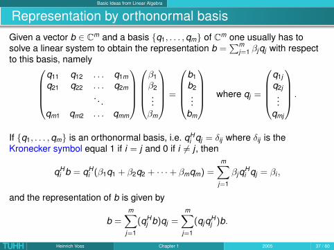
Representation by orthonormal basisGiven a vector b ∈ Cm and a basis {q1, . . . , qm} of Cm one usually has tosolve a linear system to obtain the representation b =

∑mj=1 βjqj with respect

to this basis, namelyq11 q12 . . . q1mq21 q22 . . . q2m

. . .qm1 qm2 . . . qmm

β1β2...

βm

=

b1b2...

bm

where qj =

q1jq2j...

qmj

.

If {q1, . . . , qm} is an orthonormal basis, i.e. qHi qj = δij where δij is the

Kronecker symbol equal 1 if i = j and 0 if i 6= j , then

qHi b = qH

i (β1q1 + β2q2 + · · ·+ βmqm) =m∑

j=1

βjqHi qj = βi ,

and the representation of b is given by

b =m∑

j=1

(qHj b)qj =

m∑j=1

(qjqHj )b.



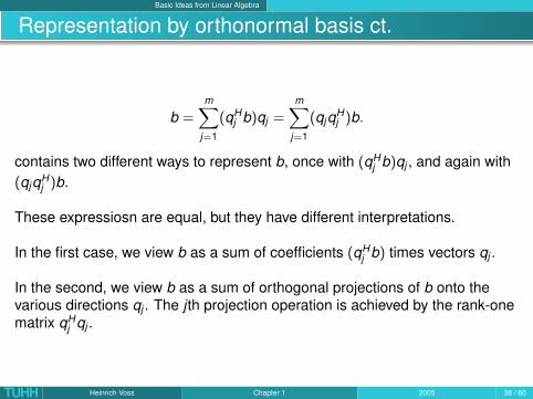
Representation by orthonormal basis ct.

b =m∑

j=1

(qHj b)qj =

m∑j=1

(qjqHj )b.

contains two different ways to represent b, once with (qHj b)qj , and again with

(qjqHj )b.

These expressiosn are equal, but they have different interpretations.

In the first case, we view b as a sum of coefficients (qHj b) times vectors qj .

In the second, we view b as a sum of orthogonal projections of b onto thevarious directions qj . The j th projection operation is achieved by the rank-onematrix qH

j qj .



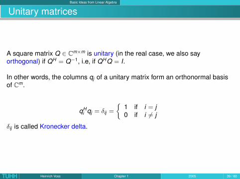
Unitary matrices

A square matrix Q ∈ Cm×m is unitary (in the real case, we also sayorthogonal) if QH = Q−1, i.e, if QHQ = I.

In other words, the columns qj of a unitary matrix form an orthonormal basisof Cm.

qHi qj = δij =

{1 if i = j0 if i 6= j

δij is called Kronecker delta.



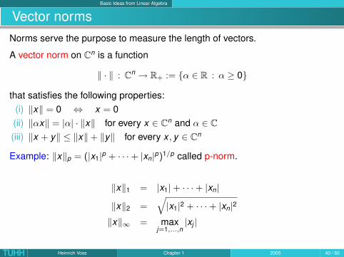
Vector normsNorms serve the purpose to measure the length of vectors.

A vector norm on Cn is a function

‖ · ‖ : Cn → R+ := {α ∈ R : α ≥ 0}

that satisfies the following properties:(i) ‖x‖ = 0 ⇔ x = 0(ii) ‖αx‖ = |α| · ‖x‖ for every x ∈ Cn and α ∈ C(iii) ‖x + y‖ ≤ ‖x‖+ ‖y‖ for every x , y ∈ Cn

Example: ‖x‖p = (|x1|p + · · ·+ |xn|p)1/p called p-norm.

‖x‖1 = |x1|+ · · ·+ |xn|

‖x‖2 =√|x1|2 + · · ·+ |xn|2

‖x‖∞ = maxj=1,...,n

|xj |



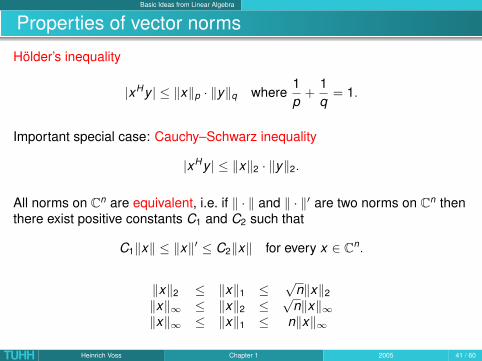
Properties of vector norms

Hölder’s inequality

|xHy | ≤ ‖x‖p · ‖y‖q where1p

+1q

= 1.

Important special case: Cauchy–Schwarz inequality

|xHy | ≤ ‖x‖2 · ‖y‖2.

All norms on Cn are equivalent, i.e. if ‖ · ‖ and ‖ · ‖′ are two norms on Cn thenthere exist positive constants C1 and C2 such that

C1‖x‖ ≤ ‖x‖′ ≤ C2‖x‖ for every x ∈ Cn.

‖x‖2 ≤ ‖x‖1 ≤√

n‖x‖2‖x‖∞ ≤ ‖x‖2 ≤

√n‖x‖∞

‖x‖∞ ≤ ‖x‖1 ≤ n‖x‖∞



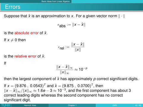
ErrorsSuppose that x is an approximation to x . For a given vector norm ‖ · ‖

εabs := ‖x − x‖

is the absolute error of x .

If x 6= 0 then

εrel :=‖x − x‖‖x‖

is the relative error of x .

If‖x − x‖∞‖x‖∞

≈ 10−p

then the largest component of x has approximately p correct significant digits.

If x = (9.876 , 0.0543)T and x = (9.875 , 0.0700)T , then‖x − x‖∞/‖x‖∞ ≈ 1.6e − 3 ≈ 10−3, and the first component has about 3correct leading digits whereas the second component has no correctsignificant digit.



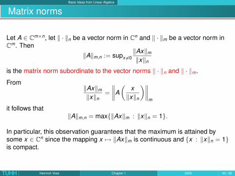
Matrix norms

Let A ∈ Cm×n, let ‖ · ‖n be a vector norm in Cn and ‖ · ‖m be a vector norm inCm. Then

‖A‖m,n := supx 6=0‖Ax‖m

‖x‖n

is the matrix norm subordinate to the vector norms ‖ · ‖n and ‖ · ‖m.

From‖Ax‖m

‖x‖n=

∥∥∥∥A(

x‖x‖n

)∥∥∥∥m

it follows that‖A‖m,n = max{‖Ax‖m : ‖x‖n = 1}.

In particular, this observation guarantees that the maximum is attained bysome x ∈ Cn since the mapping x 7→ ‖Ax‖m is continuous and {x : ‖x‖n = 1}is compact.



Properties of matrix norms

‖A‖m,n = 0 ⇐⇒ ‖Ax‖m = 0 for every x ∈ Cn

⇐⇒ Ax = 0for every x ∈ Cn

⇐⇒ A = O

‖αA‖m,n = max{‖αAx‖m : ‖x‖n = 1}= max{|α| · ‖Ax‖m : ‖x‖n = 1}= |α| · ‖A‖m,n

‖A + B‖m,n = max{‖Ax + Bx‖m : ‖x‖n = 1}≤ max{‖Ax‖m + ‖Bx‖m : ‖x‖n = 1}≤ max{‖Ax‖m : ‖x‖n = 1}+ max{‖Bx‖m : ‖x‖n = 1}= ‖A‖m,n + ‖B‖m,n

Hence ‖ · ‖m,n is a vector norm on the vector space Cm×n



Submultiplicativity of matrix norms

‖Ax‖m ≤ ‖A‖m,n · ‖x‖n for every x ∈ Cn and every A ∈ Cm×n

follows immediately from the definition of the matrix norm

For every A ∈ Cm×n and every B ∈ Cn×p it holds

‖AB‖m,p ≤ ‖A‖m,n · ‖B‖n,p.

For every x ∈ Cp

‖ABx‖m = ‖A(Bx‖m ≤ ‖A‖m,n · ‖Bx‖n ≤ ‖A‖m,n · ‖B‖n,p · ‖x‖p,

and therefore

‖AB‖m,p = max{‖ABx‖m : ‖x‖p = 1} ≤ ‖A‖m,n · ‖B‖n,p.



Geometric interpretation

The matrix norm ‖A‖m,n is the smallest nonnegative number µ such that

‖Ax‖m ≤ µ · ‖x‖n for every x ∈ Cn.

Hence, ‖A‖m,n is the maximum elongation of a vector x by the mappingx 7→ Ax with respect to the norm ‖ · ‖n in the domain Cn and ‖ · ‖m in the rangeCm

From now on we only consider the case that the same (type of) norm is usedin the domain and in the range (even if the two spaces are of differentdimensions), and we denote the matrix norm by the same symbol that is usedfor the vector norm.

Hence, if A ∈ C5×9 then ‖A‖∞ denotes the matrix norm of A with respe<ct tothe maximum norm in the domain C9 and in the range C5.



Matrix ∞-norm

‖A‖∞ = maxi=1,...,m

n∑j=1

|aij |

For every x ∈ Cn it holds

‖Ax‖∞ = maxi=1,...,m

|n∑

j=1

aijxj | ≤ maxi=1,...,m

n∑j=1

|aij | · |xj |

≤ ‖x‖∞ · maxi=1,...,m

n∑j=1

|aij |.

Thus

‖A‖∞ ≤ maxi=1,...,m

n∑j=1

|aij | (∗).



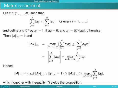
Matrix ∞-norm ct.Let k ∈ {1, . . . , m} such that

n∑j=1

|aij | ≤n∑

j=1

|akj | for every i = 1, . . . , n

and define x ∈ Cn by xj := 1, if akj = 0, and xj := akj/|akj |, otherwise.

Then ‖x‖∞ = 1 and

‖Ax‖∞ = maxi=1,...,m

|n∑

j=1

aijxj | ≥ |n∑

j=1

akjxj |

=

∣∣∣∣∣∣n∑

j=1

|akj |

∣∣∣∣∣∣ = maxi=1,...,m

n∑j=1

|aij |.

Hence

‖A‖∞ = max{‖Ay‖∞ : ‖y‖∞ = 1} ≥ ‖Ax‖∞ ≥ maxi=1,...,m

n∑j=1

|aij |,

which together with inequality (*) yields the proposition.TUHH Heinrich Voss Chapter 1 2005 48 / 60


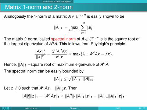
Matrix 1-norm and 2-normAnalogously the 1-norm of a matrix A ∈ Cm×N is easily shown to be

‖A‖1 := maxj=1,...,n

m∑i=1

|aij |

The matrix 2-norm, called spectral norm of A ∈ Cm×n is is the square root ofthe largest eigenvalue of AHA. This follows from Rayleigh’s principle:

‖Ax‖22

‖x‖2 =xHAHAx

xHx≤ max{λ : AHAx = λx}.

Hence, ‖A‖2 =square root of maximum eigenvalue of AHA.

The spectral norm can be easily bounded by

‖A‖2 ≤√‖A‖1 · ‖A‖∞

Let z 6= 0 such that AHAz = ‖A‖22z. Then

‖A‖22‖z‖1 = ‖AHAz‖1 ≤ ‖AH‖1‖A‖1‖z‖1 = ‖A‖∞‖A‖1‖z‖1.



Frobenius norm

For every A ∈ Cm×n it holds

‖A‖2 ≤ ‖A‖F :=

√√√√ m∑i=1

n∑j=1

|aij |2.

‖A‖F is called Frobenius norm or Schur norm

‖ · ‖F is a vector norm on Cm×n (= euclidian norm on Cm·n), but it is not matrixnorm subordinate to a vector norm, since in this case it would hold for n = mfor the unit matrix I

‖I‖ = max{‖Ix‖ : ‖x‖ = 1} = 1 whereas ‖I‖F =√

n.



Frobenius norm ct.

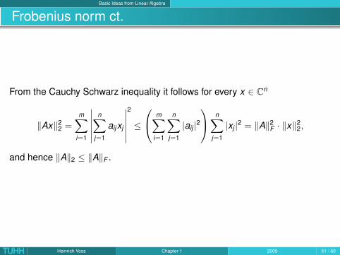
From the Cauchy Schwarz inequality it follows for every x ∈ Cn

‖Ax‖22 =

m∑i=1

∣∣∣∣∣∣n∑

j=1

aijxj

∣∣∣∣∣∣2

≤

m∑i=1

n∑j=1

|aij |2 n∑

j=1

|xj |2 = ‖A‖2F · ‖x‖2

2,

and hence ‖A‖2 ≤ ‖A‖F .



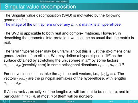
Singular value decompositionThe Singular value decomposition (SVD) is motivated by the followinggeometric fact:The image of the unit sphere under any m × n matrix is a hyperellipse.

The SVD is applicable to both real and complex matrices. However, indescribing the geometric interpretation, we assume as usual that the matrix isreal.

The term "hyperellipse" may be unfamiliar, but this is just the m-dimensionalgeneralization of an ellipse. We may define a hyperellipse in Rm as thesurface obtained by stretching the unit sphere in Rm by some factorsσ1, . . . , σm (possibly zero) in some orthogonal directions ul , . . . , um ∈ Rm.

For convenience, let us take the ui to be unit vectors, i.e., ‖ui‖2 = l . Thevectors {σiui} are the principal semiaxes of the hyperellipse, with lengthsσ1, . . . , σm.

If A has rank r , exactly r of the lengths σi will turn out to be nonzero, and inparticular, if m > n, at most n of them will be nonzero.



SVD ct.

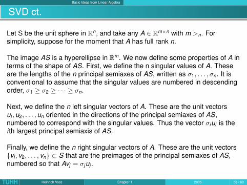
Let S be the unit sphere in Rn, and take any A ∈ Rm×n with m >n. Forsimplicity, suppose for the moment that A has full rank n.

The image AS is a hyperellipse in Rm. We now define some properties of A interms of the shape of AS. First, we define the n singular values of A. Theseare the lengths of the n principal semiaxes of AS, written as σ1, . . . , σn. It isconventional to assume that the singular values are numbered in descendingorder, σ1 ≥ σ2 ≥ · · · ≥ σn.

Next, we define the n left singular vectors of A. These are the unit vectorsul , u2, . . . , un oriented in the directions of the principal semiaxes of AS,numbered to correspond with the singular values. Thus the vector σiui is thei th largest principal semiaxis of AS.

Finally, we define the n right singular vectors of A. These are the unit vectors{vl , v2, . . . , vn} ⊂ S that are the preimages of the principal semiaxes of AS,numbered so that Avj = σjuj .



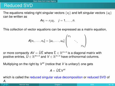
Reduced SVDThe equations relating right singular vectors {vj} and left singular vectors {uj}can be written as

Avj = σjuj , j = 1, . . . , n.

This collection of vector equations can be expressed as a matrix equation,

A[v1, . . . , vn] = [u1, . . . , un]

σ1. . .

σn

or more compactly AV = UΣ where Σ ∈ Rn×n is a diagonal matrix withpositive entries, U ∈ Rm×n and V ∈ Rn×n have orthonormal columns.

Multiplying on the right by V H (notice that V is unitary!) one gets

A = UΣV H

which is called the reduced singular value decomposition or reduced SVD ofA.



Full SVDIn most application the SVD is used in exactly the form just described.However, this is not the way in which the idea of an SVD is usually formulatedin textbooks. We have introduced the term "reduced" and the hats on U and Σin order to distinguish the factorization from the more standard "full" SVD.

The columns of U are n orthonormal vectors in the m-dimensional space Cm.Unless m = n, they do not form a basis of Cm, nor is U a unitary matrix.However, by adjoining an additional m − n orthonormal columns, U can beextended to a unitary matrix. Let us do this in an arbitrary fashion, and call theresult U.

If U is replaced by U, then Σ will have to change too. For the product toremain unaltered, the last m − n columns of U should be multiplied by zero.Accordingly, let Σ be the m × n matrix consisting of Σ in the upper n × n blocktogether with m − n rows of zeros below.

We now have a new factorization, the full SVD of A:

A = UΣV H

where U is m ×m and unitary, V is n × n and unitary, and Σ is m × n anddiagonal with positive real entries.



Full SVD ct.

Having described the full SVD, we can now discard the simplifying assumptionthat A has full rank.

If A is rank-deficient, the factorization A = UΣV H is still appropriate. All thatchanges is that now not n but only r of the left singular vectors of A aredetermined by the geometry of the hyperellipse.

To construct the unitary matrix U, we introduce m − r instead of just m − nadditional arbitrary orthonormal columns. The matrix V will also need n − rarbitrary orthonormal columns to extend the r columns determined by thegeometry. The matrix Σ will now have r positive diagonal entries, with theremaining n − r equal to zero.

By the same token, the reduced SVD also makes sense for matrices A of lessthan full rank. One can take U to be m × n, with Σ of dimensions n × n withsome zeros on the diagonal, or further compress the representation so that Uis m × r and Σ is r × r and strictly positive on the diagonal.



Formal definition of SVDLet m and n be arbitrary (not necessarily m ≥ n). Given A ∈ Cm×n, a singularvalue decomposition (SVD) of A is a factorization

A = UΣV H

where U ∈ Cm×m is unitary, V ∈ Cn×n is unitary, and Σ ∈ Cm×n is diagonal.

In addition, it is assumed that the diagonal entries σj of Σ are nonnegative andin nonincreasing order; that is, σl ≥ σ2 ≥ . . . σp, where p = min(m, n).

Note that the diagonal matrix Σ has the same shape as A even when A is notsquare, but U and V are always square unitary matrices.

It is clear that the image of the unit sphere in Rn under a map A = UΣV H

must be a hyperellipse in Rm. The unitary map V H preserves the sphere, thediagonal matrix Σ stretches the sphere into a hyperellipse aligned with thecanonical basis, and the final unitary map U rotates or reflects thehyperellipse without changing its shape.Thus, if we can prove that every matrix has an SVD, we shall have proved thatthe image of the unit sphere under any linear map is a hyperellipse.



Existence and Uniqueness

TheoremEvery matrix A ∈ Cm×n has a singular value decomposition A = UΣV H .

Furthermore, the singular values σj are uniquely determined, and, if A issquare and the σj are distinct, the left and right singular vectors {uj} and {vj}are uniquely determined up to complex signs (i.e., complex scalar factors ofabsolute value 1).

Proof: To prove existence of the SVD, we isolate the direction of the largestaction of A, and then proceed by induction on the dimension of A.

Set σ1 = ‖A‖2. By a compactness argument, there must be a vector v1 ∈ Cn

with ‖v1‖2 = 1 and ‖u1‖2 = σ1, where ul = Avl .

Consider any extensions of v1 to an orthonormal basis {vj} of Cn and of ul toan orthonormal basis {uj} of Cm, and let Ul and Vl denote the unitarymatrices with columns uj and vj , respectively.



Proof ct.

UH1 AV1 =

uH1...

uHm

A(v1 . . . vn

)=

uH1...

uHm

(Av1 . . . Avn

)

=

uH1...

uHm

(σ1u1 . . . Avn

)=

(σ1 wH

0 B

)=: S

where 0 is a column vector of dimension m − 1, wH is a row vector ofdimension n − 1, and B ∈ Cm−1×n−1.∥∥∥∥(

σ1 wH

0 B

) (σ1w

)∥∥∥∥2≥ σ2

1 + wHw =√

σ21 + wHw

∥∥∥∥(σ1w

)∥∥∥∥2

implying ‖S‖2 ≥√

σ21 + wHw .

Since U1 and V1 are unitary, it follows that ‖S‖2 = ‖A‖2 = σ1, so this impliesw = 0.



Proof ct.

If n = 1 or m = 1, we are done.

Otherwise, the submatrix B describes the action of A on the subspaceorthogonal to vl . By the induction hypothesis, B has an SVD B = U2Σ2V H

2 .

Now it is easily verified that

A = U1

(1 00 U2

) (σ1 00 Σ2

) (1 00 V2

)H

V H1

is an SVD of A, completing the existence proof.

For the uniqueness claim, the geometric justification is straightforward: if thesemiaxis lengths of a hyperellipse are distinct, then the semiaxes themselvesare determined by the geometry, up to signs.


Numerical Linear Algebra Chap. 1: Basic Concepts from ... · Numerical Linear Algebra Chap. 1:...

Documents

Transcript of Numerical Linear Algebra Chap. 1: Basic Concepts from ... · Numerical Linear Algebra Chap. 1:...