1

Numerical Laplace Transform Inversion and Selected Applications

Patrick O. Kano, Ph.D.

March 5, 2010

2

Outline The talk is organized as follows:

1. Basic definitions and analytic inversion

2. Issues in numerical Laplace transform inversion

3. Introduce three of the most commonly known numerical inversion procedures

Talbot’s Method Weeks’ Method Post’s Formula

4. Illustrate through applications Pulse propagation in dispersive materials Calculation of the matrix exponential

Future directions and conclusions

Overview

Contributions

3

Laplace Transform Definition

Laplace transform solution methods are a standard of mathematics, physics, and engineering undergraduate education.

Difficult Time Dependant

Problem

Solve SimplerLaplace Space

Problem

Time Dependant

Solution

[ ] ( ) )(0)(1

tfsFtfE LL →→=−

?

A Laplace transform is a tool to make a difficult problem into a

simpler one.

4

A sufficient existence condition is that f(t) be piecewise continuous for nonnegative values of t

of exponential order

Intuitively, the Laplace transform can be viewed as the continuous analog to a power series.

tMetf

Mt ≤≤ 0 allfor )(such that

, and enonnegativexist Thereσ

σ

Laplace Transform Definitions( ) (s)sdttfestfLsF st Re where allfor )()()()(

0

<== ∫∞

− σ

2

)(

Transform Notetf =

( ) dtetfxa st

n

ex

tfa

tn

nn

sn

−∞∞

=

=→

→→ ∫∑ →∑ ∫

−

00

)(

5

Laplace Transform Inversion How does one return from the Laplace space representation to the time

domain?

We can alleviate some of the suspense at the very beginning by cheerfully confessing that there is no single answer to this question.

Instead, there are many particular methods geared to appropriate situations.

This is the usual situation in mathematics and science and, hardly necessary to add, a very fortunate situation for the brotherhood.

Richard Bellman

6

Analytic Inversion The analytic inversion of the Laplace transform is a well-known application

of the theory of complex variables. For isolated singularities, the Bromwich contour is the standard approach.

∫∞+

∞−

=i

i

stdsesFi

tfσ

σπ)(

2

1)(

Realσ

Abscissa of convergence

Isolated singularities

Imaginary

Laplace transform inversion is not a unique operation. In practice, one can assume that the analytic inverse is well-defined.

Lerch’s theorem

( )( ) ( )

( ) ( ) 0 ,0 allfor then,

)(

transformLaplace same thehave and )(function twoif

2

0

1

21

21

=−>

=≡

∫ dttftf

fLfLsF

tftf

τ

τ

7

Numerical Inversion Issues The numerical inversion of the Laplace transform is an inherently ill-

posed problem.

To combat these numerical issues one may use 2 tactics

1. Fixed-point high precision variables.

2. Use of multiple algorithms, each with efficacy for certain classes of functions.

∫Λ

= dsesFi

tf st)(2

1)(

π

Inherent sensitivity due to the multiplication by a exponential function of time.

Algorithmic and finite precision errors can lead to exponential divergence of numerical solutions.

8

Mathematica ARPREC

An Arbitrary Precision Computation Package Lawrence Berkley National Laboratory D. Bailey, Y. Hida, X. Li, B. Thompson

Fixed-Point High Precision Variables

High precision variables are required for most inversion methods.

This requirement is important consequences: Numerical LT methods are typically slower than other time-

propagation methods. Implementation requires either

An environment where high precision variables are innate. Additional high precision variable software packages.

Double Precision: 10-308-10308

GMP GNU Multiple Precision Arithmetic

Library MP

Matlab Based Toolbox Ben Barrows Matlab file exchange

10308~e709σ Large for even modest times.

9

Numerical Inversion

Post’s Formula Alternative to integration; arises from Laplace’s method Post (1930), Gaver (1966), Valko-Abate (2004)

The Weeks method Laguerre polynomial expansion Ward (1954), Weeks (1966), Weideman (1999)

Fourier series expansion Fourier related method Koizumi (1935), Dubner-Abate (1968), DeHoog-Knight-Stokes (1982),

D’Amore (1999) Talbot’s method

Deformed contour method Talbot (1979), Weideman & Trefethen (2007)

Euler1707-1783

Laplace1749-1827

Heaviside1850-1925

Time

Post1930

Weeks1966

FourierSeries1968

Talbot1979

10

Talbot’s Method (1979) Talbot’s method is based on a deformation of the

Bromwich contour. The idea is to replace the contour with one which

opens towards the negative real axis.

Talbot’s method requires that

( ) jj sKs

ssF

iessingularit allfor Im

as 0)(

<∞→→

( ) ( )

πθπσνλ

θνλ θσθ

<<

++=

-

real are ,,

cotis

11

Talbot’s Method The method is easily implemented in Mathematica.

0.39140

0.04710

0.14120

1.62580

Run TimePrecision

3

/12 )()(

t

etfesF

ts

π

−− =↔=

1 , ,0 21 === νλσ

( ) ( )

( )[ ]

θθπ

θθθθλλθ

πθπνσπθνλ θσθ

π

π

dd

dssFe

itf

id

ds

is

st∫−

=

−+−=

<<==++=

)(2

1)(

cot1cot

-,1,0

cot

The Talbot method answers are accurate up-to the computation precision for time t=1.

Timeval = 1;

Rval = 1/2;

Flap[s_]=Exp[­2*Sqrt[s]];

Tfunexact[t_] =Exp[­1/t]/Sqrt[Pi*t*t*t];

Valexact = N[Tfunexact[Timeval],1000]

STalbot[r_,a_]=r*a*Cot[a]+I*r*a;

dsda[r_,a_]=I*r*(1+I*(a+Cot[a]*(a*Cot[a]­1)));

TimeDfun[r_,t_]:=1/(2*Pi*I)*NIntegrate[Exp[STalbot[r,a]*t]*Flap[STalbot[r,a]]*dsda[r,a],{a,­Pi,Pi},WorkingPrecisionŁ20];

{Timeval,Approxval}=Timing[TimeDfun[Rval,Timeval]]

RelError = Abs[Approxval­Valexact]/Valexact

12

Talbot’s Method

Attempts have been made to automate the selection: “Algorithm 682: Talbot’s method of the Laplace inversion problems”,

Murli & Rizzardi, 1990. [FORTRAN]

This is an active area of research. Optimizing Talbot’s contours for the inversion of the Laplace

transform, A. Weideman, 2006 Parabolic and Hyperbolic contours for computing the Bromwich

integral, A. Weideman & L.N. Trefethen, 2007

The primarily difficulty lies in the selection of appropriate values for the contours parameters.

( )2cos)(2

)(2

ttfs

ssF =↔

+=

1 , ,0 21 === νλσ

Mathematica’s adaptive integration fails for the same parameter values.

13

Post’s Formula (1930)

There are two features of Post’s formula which are particularly attractive It contains no parameters, save the order of the derivative and the

precision of the computations. The inversion is performed using

Only real values for s Without priority knowledge of poles

Post’s formula manifests the same inherent ill-posedness from which all numerical inversion procedures suffer. Errors are amplified multiplicative factor grows quickly with the order of

the derivative q The method converges slowly One needs an expression or approximation for the higher order derivatives

of F(s)

( )tqs

q

qqq

qsF

ds

d

t

q

qtf

/

1

)(!

1lim)(

=

+

∞→

−=

Emil Post’s inversion procedure provides an alternative to Bromwich contour integration

14

Derivation Post’s formula can be

derived using Laplace’s method

( ) ( )

( ) ( )0

2

20

0

2

2

0

0

00

k

2~)I(k,

behaviour asymptotic thehas

I(k)

integral the,k as

then,0 if and0 if

τπτ

ττ

τ

τ

τ

ττ

he

dτgd

dhe

dτ

gd

dτ

dg

kg

kg

−

∞−∫=

∞→

≠=

( )

( ) ( )

( ) ( ) ( )

( ) ( ) ( )

( ) ( )

( )

( )

+++

−

+++=

−

−

=−===

=−

=

−=

=

+

−

−+

−−

∞−

∞−

∞−

∫

∫

∫

2

1

2

1

ln12

22

2

0

0

/ln

0

0

288

1

12

11)(

!

1~)(

288

1

12

112k!

formula sStirling'With

)(k2~)(1

)(2

~)(1

1

d

gd ,ln/ , ,Assign

)(1

at evaluate and Rearrange

1)(

respect to with derivative theTake

)(

0

kktkF

t

k

ktf

kkkek

tfetkF

t

k

tfek

tt

kF

ttgfht

dfetkF

tks

dfesF

sk

dfesF

kkk

kk

kkk

k

tkkk

tkkk

skkk

th

s

π

π

π

τττττττ

ττ

τττ

ττ

τ

ττ

τ

τ

Approximate

15

Derivatives Finite differences an obvious method by which to approximate the

derivatives of a reasonably behaved function.

The Gaver functionals can be computed by a recursive algorithm:

( )

( ) ( )( ) ( )

( ) ( )

)(lim)(

)2ln(2)2ln()(

1

)2ln(2)2ln(1)(

01

tftf

tjqF

j

q

q

q

tqtf

nxFxnFnxF

tqF

q

q

tqtf

qq

q

j

j

q

qqq

∞→

=

=

+

=

−+=∆

∆

−=

∑ −

Gaver-Post Formula1966

( )

( ) ( ) ( ) np p,1 1G

n1 2ln2ln

111

np

0

≤≤

−

+=

≤

=

+−−n

pn

p

n

Gp

nG

p

n

tnF

tnG

qqGtf =)(q

16

Derivatives Post’s formula does not require a finite difference

approximation. For a particular function form, e.g. composition of two

functions, a tailored method may be more robust.

( )

( ) qqq

m

m

q

q

pmqm

mpq

mpq

pq

pq

q,p

q

pp

p

q

q

xgB

dx

gdB

qB

B

Bdx

gd

m

qB

dx

gd,,

dx

gd,

dx

dgBg(x)

dx

fdf(g(x))

dx

d

)(

1for 0

1

1

1

,

1,

0,

0,0

1,

1

1,

1

1

2

2

0

=

=

≤==

−−

=

=

−−

+−

=

+−

+−

=

∑

∑

Bell Polynomials of the Second Kindwww.mathworks.com/matlabcentral/fileexchange/14483

Faa di Bruno’s formula

17

Acceleration Sequence acceleration methods be used to greatly increase accuracy

The proper application of an acceleration convergence method requires some additional knowledge about the series.

Post’s formula is logarithmically convergent

Slow Sequence {fq(t)}

Linear or NonlinearTransform

Fast Sequence {hq(t)}

<<=

−

−=

∞→

+

eConvergencLinear 10

eConvergenc cLogarithmi1lim

)()(

)()( 1

ca

tftf

tftfa

qq

q

q

q

11

lim)()(

)()(lim

)()()(~)(

1

211

=+

=−

−

+++

∞→

+

∞→ q

q

tftf

tftf

q

tc

q

tctftf

qq

q

q

q

Gaver (1966)

18

Acceleration Wynn-rho algorithm is well suited to logarithmically convergent

sequences. Studies have shown that it is useful for the Post formula:

NSum in Mathematica implements these acceleration methods.

Post Inversion Formula and Sequence AccelerationUA VIGRE Project 2009J. Cain & B. Berman

11

01

1

21

32

22

212

20

21

12-Q

12

111

10

11

02-Q

02

010

00

01

02-Q

0

0

0

0

by Q,even for ,lim)(

function for theion approximatan yields algorithm The

−−−

−

−

−

−

−

−

∞→

==

======

=

QQQ

Q

Q

qq

f

f

f

f

ftf

ρρρ

ρ

ρρρρρρρρρρρρρρ

ρ

kQq

Qk

k qkq

kqk

qk

−−=−=

+−+= +

−++

1,,0

3,,0

1 1111

ρρρ

ρ

￤ " A l t e r n a t i n g S i g n s " m e t h o d f o r s u m m a n d s w i t h a l t e r n a t i n g s i g n s

" E u l e r M a c l a u r i n " E u l e r | M a c l a u r i n s u m m a t i o n m e t h o d

" W y n n E p s i l o n " W y n n e p s i l o n e x t r a p o l a t i o n m e t h o d

19

Application of Post’s Formula

Rapid computation of the distribution of an initial optical pulse in a fixed dielectric medium with a nontrivial material dispersion relation.

NSF Grant ITR-0325097An Integrated Simulation Environment for High-Resolution Computational Methods in Electromagnetics with Biomedical ApplicationsMoysey Brio, et. al.

( )srε

Material

Biological materials often have a dielectric constantwhich is a complex function of wavelength.

Input Pulse of Light Out Pulse of a Different Shape

Create databases of pre-computed tables which can be used by devices which must operate in real-time.

20

Cole-Type Dispersion Relation Many real world materials can be described by a Cole-type dispersion model.

( )[ ]{ }{ }{ }

( ){ }( )

( )∞∈∞∈∞∈

∞∈∈∈

++

+=

∞

−∞ ∑

,0

,0

,0

),0[

]1,0(

)1,0[

1)(

01

σετδ ε

εσ

τδ εεε

n

n

n

n

nba

n

nr

b

a

sss

nn

02.0

958.7)(

105.3

30.0

05.53)(

100.4

10.0

96.7)(

0.100

10.0

96.7)(

0.32

4

4

74

3

3

43

2

2

2

1

1

1

==

⋅=

==

⋅=

==

==

==

a

ms

a

ns

a

ns

a

ps

τδ ε

τδ ε

τδ ε

τδ εBrain

White Matter

A standard method used in computational optics is to incorporate the dispersion relation by means of an associated difference equation.

For fractional coefficients, it is not clear how to translate into an associated equation.

Fractional aCoefficients

{ } 1

02.0

0.4

===∞

b

σε

21

Maxwell’s equations are the starting point for this analysis.

In the Laplace space, the convolution and derivatives become multiplications.

( )( )

( ) ( )

( ) ( )

( ) ( ) ( ) ( ) τττεε

µ

dxEttxEtxD

DE

txt

HtxE

txt

DtxH

txH

txD

t

,,,

nt displaceme theand strength field electricbetween assumption General

,,

,,

0,

0,

0

00

0

k

∫ −Φ+=

∂∂−=×∇

∂∂=×∇

=⋅∇=⋅∇

Maxwell’s Equations

Temporal Convolution

( ) )()()(0

sGsFdtgfLt

=

−∫ τττ ( ) ),()(),(

0

sxEsdtxELt b

φτττ =

−Φ∫

22

Maxwell’s equations now have a simpler form.

Eliminating the magnetic field H from the problem,

One obtains the wave equation in Laplace space

Maxwell’s Equations( ) ( ) ( )

( )( )

( ) ( ) ( ) ( )( ) ( ) ( )( )0,,,

0,,)(1,

0,

0,

,)(1,

0

00

0

=−−=×∇

=−+=×∇=⋅∇=⋅∇

+=

txHsxHssxE

txEsxEsssxH

sxH

sxE

sxEssxD

p

µεφε

φε

( ) )0,()0,(),()(1),( 00000022 =

∂∂−=−=+−∇ tx

t

EtxEssxEsssxE

à

εµεµφεµ

( ) ( ))0,()0,( 0

2

=∂∂==×∇

∇−⋅∇∇=×∇×∇

txt

EtxH

HHH

¸

ε

23

One can more succinctly state this last equation as

Applying a Fourier transform yields the desired solution in the joint space

002

22

22

1 )(1)(

)0,()0,(),(

),(1

),()(),(

µεφε

ε

=+=

=∂∂+==

−=−∇

css

txt

EtxEssxV

sxVc

sxEsc

ssxE

r

r

�

Maxwell’s Equations

222 )(

),(),(

kcss

skVskE

r

è

+=

ε

24

Database Coefficients in the Joint Space The solution in a dielectric medium can be characterized by one

coefficient α and its time derivative.

Compute high order derivatives of α(k,s) and β(k,s) beta derivatives are trivially obtain from the alpha derivatives.

( ) ( )( ) ( ) ( )skssk

kcsssk

tkEt

sktkEskskE

r

,, )(

1,

)0,(,)0,(,),(

222

è

αβε

α

αβ

=+

=

=∂∂+==

For a given dispersion relation εr(s), the coefficients are pre-computed and stored in a matrix of k vs time.

( ) ( ) ( )skqDsksDskD qqq ,,, 1ααβ −+=

The crux of the problem is the arbitrary precision calculation of the q-th derivative of α .

25

Derivative Approaches1.1. Standard Gaver-Wynn-RhoStandard Gaver-Wynn-Rho

Finite Differences + Wynn-Rho Acceleration A brute force application entails a computation for each k and s.

Gaver-PostGaver-Post Finite Differences + Wynn-Rho Acceleration The arbitrary precision computation of the dispersion relation εr(s) is

time consuming. Dispersion relation is independent of k More efficient to store εr(s) and call for each k evaluation of α.

Bell-PostBell-Post Analytic Derivatives + Wynn-Rho Acceleration Store εr(s) and its derivatives. Use Faa di Bruno’s formula for the qth derivative of the computation of

two functions.

( ) ( )

+=

= ∑ −

= tjqsk

j

n

q

q

tqtk

q

j

j

q

)2ln(,

2)2ln(),(

01 αα

26

Bell-Post Method The problem of determining the time dependence of α(k,t) and thus

the electric field is reduced to evaluating the susceptibility function and its arbitrary order derivatives.

( )

( )

( )( )

( )[ ] ( )

( ) ( ) ( )sDnnssnDsDssgD

sgDsgDsDgBkcss

pskD

kcsssg

ssf

dx

gd,,

dx

gd,

dx

dgBg(x)

dx

fdf(g(x))

dx

d

kcsssk

rn

rn

rnn

q

p

pqpqp

r

pq

r

pq

pq

q,p

q

pp

p

q

q

r

εεε

εα

ε

εα

212

0

12,1222

222

1

1

2

2

0

222

)1(2)(

Rule Leibniz

)(,),(),(1!

),(

)(

1)(

)(

1,

−−

=

+−+

+−

+−

=

−++=

+−=

+=

=

=

+=

∑

∑

27

Cole-Type Dispersion Relation For white brain matter the derivatives of εr(s) can be found by using the

Faa di Bruno formula.

( )[ ]{ }{ }{ }

( ){ }( )

( )∞∈∞∈∞∈

∞∈∈∈

++

+=

∞

−∞ ∑

,0

,0

,0

),0[

]1,0(

)1,0[

1)(

01

σετδ ε

εσ

τδ εεε

n

n

n

n

nba

n

nr

b

a

sss

nn

( ) ( )

( )( )

( ) ( )

( )

( ) ( ) ( )kbk

j

kk

pap

j

ap

kqkq

q

k

kq

q

b

a

nn

q

q

nq

q

qr

q

gjbgf

sjasg

sgggBsgfds

sgfd

ssf

ssg

sgfds

d

s

q

ds

sdn

+−−

=

−−−

=

−

+−

=

−

−

+

+

+−=

−−=

=

+=

=

+−=

∏

∏

∑

∑

1)1()(

1)(

)(,,,)())((

1)(

)(

)(!1)(

1

0

11

0

1

121,

0

1

10

τ

τ

δ εεσε

28

Mathematic Implementation Flow DiagramInputs

• Choose [qmin,qmax]• Inversion time t• Take an explicit expression for εr(s) and its derivatives• A set of wavenumber k

Evaluate εr(s) and its derivatives at s=q/t

Compute s2εr(s) and its derivatives via Leibniz’s rule

Compute the Bell polynomials from the recursion relation

For k, compute s2εr(s) + c2k2

Compute the qth and (q-1)th derivatives of α(k,s)

Compute the qth derivative of β(k,s)

Approximate the inversion coefficients via Post’s formula

Apply Wynn-rho acceleration

Repeat for each q

29

Brain White Matter: Run Time

The Bell-Post and Gaver-Post methods are faster than a standard Gaver. The acceleration dominates over the sequence computation times. The time follows a polynomial growth with q-max.

Time=(16/3)t0

100 Digits Precision

pAqT =

1.6550.148Brute

Gaver

1.438-0.189Gaver-Post

1.670-0.592Bell-Post

pLog ACase

30

Brain White Matter: Accuracy

Time=(16/3)t0

100 Digits Precision

The Bell-Post and Gaver-Post methods have comparable accuracy At higher precision and Post formula derivative orders.

31

The Weeks Method (1966) The Weeks’ method is one of the most well known algorithms for the

numerical inversion of a scalar Laplace space function. It popularity is due, in part, to the fact that it returns an explicit

expression for the time domain function. The Weeks method assumes that

a smooth time domain function of bounded exponential growth can be expressed as the limit of an expansion in scalar Laguerre

polynomials.

( )

( )

( ) ( )nxn

nx

n

N

nn

btn

tN

NN

xedx

d

n

exL

btLeaetf

tftf

−

−

=

−

∞→

=

=

=

∑

!

2)(

)(lim

1

0

σThe coefficients {an}

2. contain the information particular to the Laplace space function

3. may be complex scalar, vectors, or matrices

4. time independent

32

The Weeks Method Two free scaling parameters σ and b, must be

selected according to the constraints that b>0 ensures that the Laguerre polynomials are well

behaved for large t σ>σ0-abscissa of convergence

Laguerre Polynomials

33

The Weeks Method The computation of the coefficients begins with a

Bromwich integration in the complex plane.

Assume the expansion

Equate the two expressions

( )∫∞

∞−

+=

∞<<∞>+=

dyiyFee

tf

iys

iytt

σπ

σσσσ

2)(

y- , , 0

( )∑∞

=

−=0

2)(n

nbt

nt btLeaetf σ

( ) ( )∫∑∞

∞−

∞

=

− += dyiyFebtLea iyt

nn

btn σ

π2

12

0

34

Key Weeks Method Facts It is known that the weighted Laguerre coefficients have the

Fourier representation.

Performing the appropriate substitution, assuming it is possible to interchange the sum and integral equating integrands leaves

( ) ( )( )∫

∞

∞−+

−

+−= dybiy

biyebtLe n

niyt

nbt

12

12

π

( )( ) ( )∑

∞

=+ +=

+−

01

nn

n

n iyFbiy

biya σ

35

Moebius Transformation One may apply a transformation from complex

variable s to a new complex variable w

biy

biywiyσs

bs

bsw

+−=+=

+−−−= , or with

σσ

Isolated singularities of F(s) in the s-half-plane are mapped to the exterior of the unit circle in the w-plane.

36

W-plane Representation With the change of variables, one obtains

a power series in w whose radius of convergence is greater than 1.

The function is analytic on the unit circle.

Numerically, the evaluation of the integral can be computed very accurately using the midpoint rule

−+−

−=∑

∞

= 1

1

1

2

0 w

wbF

w

bwa

n

nn σ

θσπ

π

πθ

θ

θθ d

e

ebF

e

bea

i

i

iin

n ∫−

−

−+−

−=

1

1

1

2

2

1

M

m

e

ebF

e

be

M

ea m

M

Mmi

i

iin

Min

n m

m

m

mπθσ θ

θ

θθ

π

=

−+−

−≈ ∑

−=

−−

+

+

+

1

1

1

2

2 2/1

2/1

2/1

2

37

Matrix Exponential Application An application of the Weeks method is to the

calculation of the matrix exponential.

00 )(0 , xetxx)(tx xAdt

xd At @

=→===What does it mean “the

exponential of a matrix”?

++++=!3!2

32 AAAIeA

Why don’t we just calculate this?

“Nineteen Dubious Ways to Compute the Exponential of a Matrix”,SIAM Review 20, C. B. Moler & C. F. Van Loan, 1978.

“Nineteen Dubious Ways to Compute the Exponential of a Matrix, Twenty-Five Years Later”, SIAM Review 45, C. B. Moler & C. F. Van Loan, 2003.

Inverse Laplace Transform (#12)

[ ]∫ −−=Bromwich

At AsIi

e dse2

1 st1

π Resolvent Matrix of A

Apply the Weeks method

38

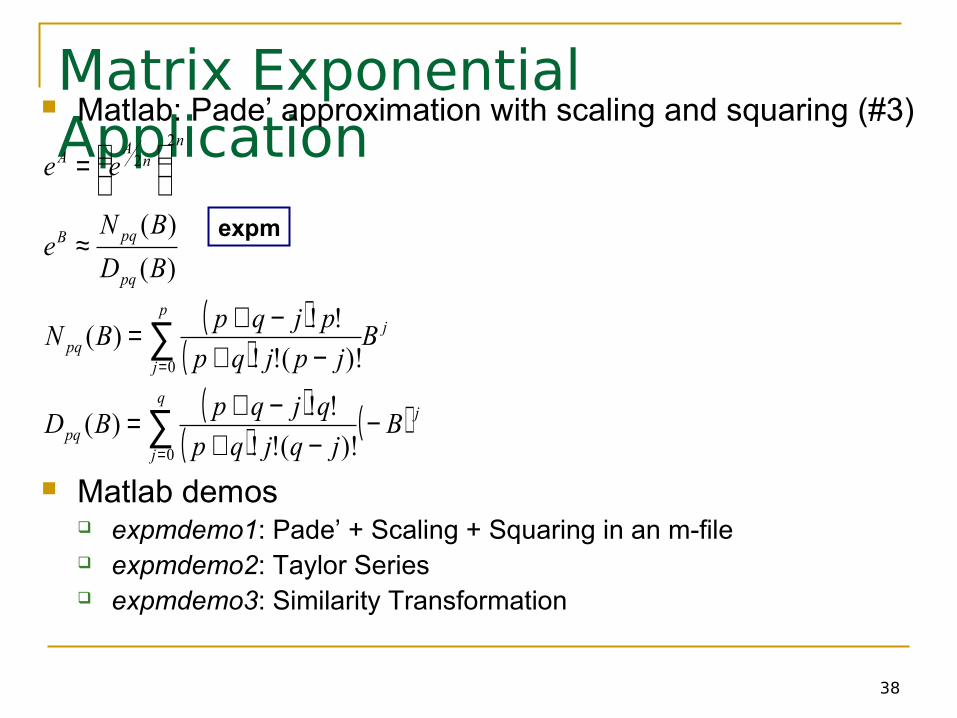
Matrix Exponential Application

Matlab: Pade’ approximation with scaling and squaring (#3)

Matlab demos expmdemo1: Pade’ + Scaling + Squaring in an m-file expmdemo2: Taylor Series expmdemo3: Similarity Transformation

( )( )

( )( ) ( ) j

q

jpq

jp

jpq

pq

pqB

nn

AA

Bjqjqp

qjqpBD

Bjpjqp

pjqpBN

BD

BNe

ee

−−+

−+=

−+−+=

≈

=

∑

∑

=

=

0

0

22

)!(!!

!!)(

)!(!!

!!)(

)(

)( expm

39

Beam Propagation Equation Nonparaxial scalar beam propagation equation

Discretisation in space yields a set of ODEs

The Laplace transform in z yields

uzyxnkx

iuiz

u

+

∂∂−=

∂∂

),,(2202

2

β

( )uzyxnkDiuiz

u),,(22

0+−=∂∂ β

( )[ ] ( )

2

2220

1 0)(ˆ

ββ

βInkD

A

uAIIisIsu

−+=

+−−=− ð

u = a component of the electric field

40

Beam Propagation Equation The Laplace space function is of a matrix exponential

The issue is how to pick the Laguerre polynomial parameters σ and b. Weeks’ original suggestions

Error-Estimate Motivated Approach Weideman Method

minimization of the error estimate as a function of σ and b

Min-Max Method Maximum the radius of convergence as a function of σ and b

[ ] ( ) ( )[ ]∫ −

−

−=

+−=−=

Bromwich

Mt MsIi

e

AIIiMuMsIsu

dse2

1

0)(ˆ

st1

1

π

β€

tcoefficienexpansion #21

0max 0 ==

+= N

t

N b

t,σσ

Expensive Matrix

Inversions

41

Error Estimates A straight forward error estimate yields three contributions

Discretisation error: Finite integral sampling Truncations error: Finite number of Laguerre polynomials Round-off error: Finite computation precision

+≤ ∑∑

−

=

∞

=

1

0

22N

nFn

NnFn

ttotal aaeE εσ

Truncation Round-Off

Weideman Method

Min-Max Method

Midpoint rule on circular contour

( )1

)(

)()(

2

1

1

1

2

−≤

=≤

−

=+∫

rr

rKT

r

rKdw

w

rKa

NE

nrw

nFn π( )

radiuscontour circular plane-wr

matrixresolvent theof norm

==rK

42

Beam Propagation Equation Example Multi-mode interference coupler

Maximum

Solution

Absolute Error

bσ

Weideman

Min-Max

Weeks

0.00042516.7911.84

0.001191020

12.28321

By proper selection of the parameters, it is possible to perform the calculations in double precision.

43

Pathological Matrices An application is the exponential of special matrices.

6x6 Pei MatrixMaximum Element Relative Error

32 Coefficients

2 1 1 1 1 11 2 1 1 1 11 1 2 1 1 11 1 1 2 1 11 1 1 1 2 11 1 1 1 1 2

Weeks’

MinMax(2 Search Methods)

Weideman Eigenvalues 1N+1 (7)

gallery(‘pei’,6)

www.math.arizona.edu/~brio/WEEKS_METHOD_PAGE/pkanoWeeksMethod.html

44

Future Directions

NLAP-CL: Robust Parallel Numerical Laplace Transform Inversion via a C-CUDA Library and Application to Optical Pulse Propagation•Mosey Brio – University of Arizona•Patrick Kano – Applied Energetics, Inc.•Paul Dostert – Coker College

Extend NSF supported Post’s Formula Work to 2D and 3D

Mathematica is too slow.

(CUDA)NVIDIA’s Compute Unified Device Architecture

December 2009 – NSF proposal submitted

Tables of coefficients for

multiple dispersive materials

NLAP requires multiple simple arithmetic computations in high precision.

MATLAB C-MEX Files MATLABNLAP

Front End

45

Summary & Conclusions The purpose the of the presentation was to provide some insight and

illustrate applications of numerical Laplace transform inversion.

Standard methods Talbot’s Method Post’s Formula The Weeks method

Illustrated two examples Calculation of the matrix exponential Optical pulse propagation in dispersive media

Numerical Laplace transform inversion is a topic multitude of nuances to provide avenues for further research popularity increase as computing power improves potential for practical application in diverse fields

Great utility and intellectual merit to the development of a general numerical Laplace inversion toolbox.

46

Sources Numerical Inversion of the Laplace Transform, Bellman, Kalaba, Lockett, 1966.

Peter Valko’s NLAP website: www.pe.tamu.edu/valko/public%5Fhtml/NIL/

“Numerical inversion of Laplace transforms using Laguerre functions”, W. Weeks, Journal of the ACM, vol. 13, no. 3, pp.419-429, July 1966.

“The accurate numerical inversion of Laplace transforms”, J. Inst. Math. Appl., vol. 23, 1979.

“Application of Weeks method for the numerical inversion of the Laplace transform the matrix exponential”, P. Kano, M. Brio, J. Moloney, Comm. Math. Sci., 2005.

“Application of Post’s formula to optical pulse propagation in dispersive media”, P. Kano, M. Brio, Computers and Mathematics with Applications, 2009.

47

BACKUPS

BACKUP

48

Laguerre Polynomials An unstable approach to obtain the time domain

function is to generate the Laguerre polynomials is to use the recurrence relation

A backward Clenshaw algorithm is a stable method.

( ) ( )

( ) ( )∑∞

=

−

−+

=

−==

−−+=+

0

1

0

11

2)(

1)(

1)(

)()(12)(1

nnn

tb

nnn

btLaetf

xxL

xL

xnLxLxnxLn

σ

49

Analytic Inversion

( )[ ]2order 0

1

1)(

2

2

=

=

=

s

es

sg

ssF

st( ) ( ) ( )[ ]

ttees

sds

dr

sgssds

d

!mr

πirdses

t

s

st

ss

m

m

m

iσ

iσ

st

==

=

−−

=

=

=

=−

−

∞+

∞−∫

0

02

2

01

1

2

1

1

1

21

0

ts

Ltf

tdsesi

i

i

st

=

=

=

−

∞+

∞−∫

21

2

1)(

1

2

1 σ

σπ

50

Application of Post’s Formula Post’s formula was implemented to

invert the Fourier-Laplace space coefficients which arise from the solution of the optical dispersive wave equation.

We considered three implementations Standard Gaver-Wynn-Rho Gaver-Post Bell-Post

51

Brain White MatterRelative Error, Bell-Post, k=kmax Relative Error, Gaver-Post, k=kmax

The Bell-Post method performs well at modest values for the

precision and order of the Post formula approximation.

At higher precision and Post formula approximation order, the Gaver-Post has an accuracy/unit run time comparable or

better than the Bell-Post method.