Procedia CIRP 10 ( 2013 ) 37 – 43

Available online at www.sciencedirect.com

2212-8271 © 2013 The Authors. Published by Elsevier B.V.Selection and peer-review under responsibility of Professor Xiangqian (Jane) Jiangdoi: 10.1016/j.procir.2013.08.010

ScienceDirect

12th CIRP Conference on Computer Aided Tolerancing

Numerical investigation into the impact of dimensional and geometric tolerances on the long-life fatigue strength of mechanical

components

Peter Gust*, Christoph Schluer Chair of Engineering Design, University of Wuppertal, Gaußstr. 20, 42651 Wuppertal, Germany

Abstract

Complex assemblies need to address ever-increasing cost-efficiency requirements. Therefore it is necessary to max out permissible stresses during the design process. In addition, there is a need to match estimated lifetimes more and more exactly, so it is important to predict accurately the effective stresses on mechanical parts. This paper examines the impact of size and geometric tolerance on stress and long-life fatigue strength. For this purpose an in-house software tool has been developed which makes it possible to generate a CAD model with simultaneous consideration of all geometric tolerances. The resultant model has a stochastically deformed shape but still corresponds to its engineering drawing. In a second step an FE analysis is performed to determine the influence of these tolerances on the long-life fatigue strength of the parts. These results are compared with the results for the model without the geometric tolerances (using only nominal CAD data). © 2012 The Authors. Published by Elsevier B.V. Selection and/or peer-review under responsibility of Professor Xiangqian Jiang.

Keywords: geometric tolerancing; elastic tolerance analysis; long-life fatigue strength; non-ideal geometry; deformed CAD

1. Introductiona

CAD data and derived geometrical models are perfect. The geometry is based on nominal dimensions. Deviations that are smaller than the permitted dimensional and geometrical tolerances are not modelled. State-of-the-art computer-based methods are available for analysing the tolerances and function of a new product. Typical software systems work with rigid bodies (e.g. VisVSA, a software tool for 3D tolerance analysis). To recognise physical effects like elasticity, it is necessary to use more complex software tools like optiSLang (a software tool for robust design and

* Corresponding author. Tel.: +49-202-439-2046; fax: +49-202-439-2048 . E-mail address: peter.gust@uni-wuppertal.de.

parameter studies). Those software tools use Monte Carlo or Latine Hyper Cube schemes to change the nominal dimensions systematically and calculate the resulting functional dimensions, or e.g. the output parameters, of an FEA. The result is not a single value; instead you get a statistical average value and limits of variation. It is also possible, through a sensitivity study, to determine the main parameters that influence the output parameter. For the calculation of a one-side-fixed rectangular beam with a single load applied, you will find that height is the main parameter for minimal bending. This result is obvious to an engineer, but the result is not so easy to guess for more complex systems. In Fig. 1 you can see a workflow for this method.

© 2013 The Authors. Published by Elsevier B.V.Selection and peer-review under responsibility of Professor Xiangqian (Jane) Jiang

Open access under CC BY-NC-ND license.

Open access under CC BY-NC-ND license.

38 Peter Gust and Christoph Schluer / Procedia CIRP 10 ( 2013 ) 37 – 43

= 2 ( ( )( ) )²=1 ( ( ) )²=1( | {1, … , } i { }).

.

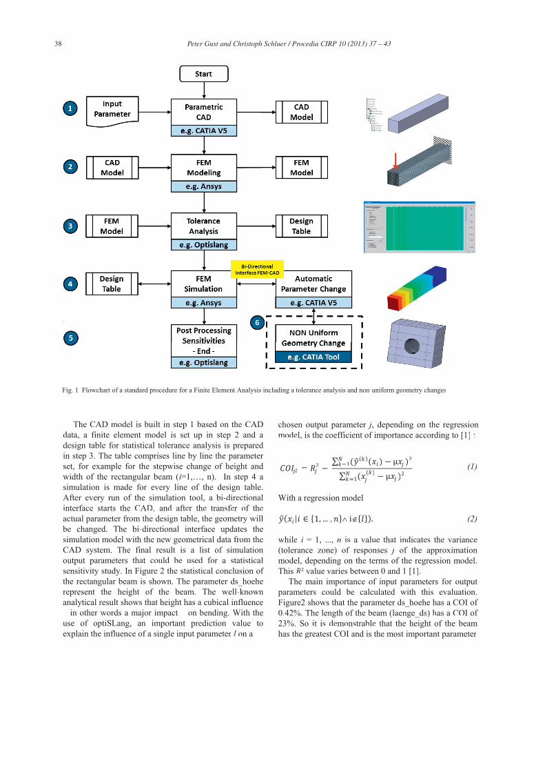
The CAD model is built in step 1 based on the CADdata, a finite element model is set up in step 2 and a design table for statistical tolerance analysis is prepared in step 3. The table comprises line by line the parameter set, for example for the stepwise change of height and width of the rectangular beam (i=1,…, n). In step 4 a simulation is made for every line of the design table. After every run of the simulation tool, a bi-directionalinterface starts the CAD, and after the transfer of theactual parameter from the design table, the geometry willbe changed. The bi-directional interface updates thesimulation model with the new geometrical data from the CAD system. The final result is a list of simulationoutput parameters that could be used for a statisticalsensitivity study. In Figure 2 the statistical conclusion of the rectangular beam is shown. The parameter ds_hoeherepresent the height of the beam. The well-known analytical result shows that height has a cubical influence– in other words a major impact – on bending. With theuse of optiSLang, an important prediction value toexplain the influence of a single input parameter l on a

chosen output parameter j, depending on the regressionmodel, is the coefficient of importance according to [1] :

(1)

With a regression model

(2)

while i = 1, ..., n is a value that indicates the variance (tolerance zone) of responses j of the approximationmodel, depending on the terms of the regression model.This R² value varies between 0 and 1 [1].

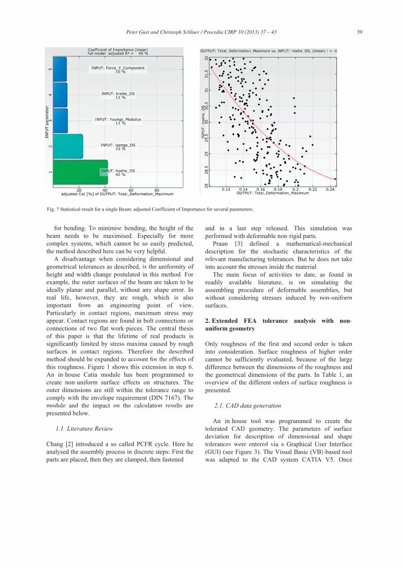
The main importance of input parameters for output parameters could be calculated with this evaluation.Figure2 shows that the parameter ds_hoehe has a COI of0.42%. The length of the beam (laenge_ds) has a COI of 23%. So it is demonstrable that the height of the beam has the greatest COI and is the most important parameter

Fig. 1. Flowchart of a standard procedure for a Finite Element Analysis including a tolerance analysis and non-uniform geometry changes

39 Peter Gust and Christoph Schluer / Procedia CIRP 10 ( 2013 ) 37 – 43

for bending. To minimise bending, the height of thebeam needs to be maximised. Especially for morecomplex systems, which cannot be so easily predicted,the method described here can be very helpful.

A disadvantage when considering dimensional and geometrical tolerances as described, is the uniformity of height and width change postulated in this method. For example, the outer surfaces of the beam are taken to be ideally planar and parallel, without any shape error. Inreal life, however, they are rough, which is alsoimportant from an engineering point of view.Particularly in contact regions, maximum stress mayappear. Contact regions are found in bolt connections or connections of two flat work-pieces. The central thesisof this paper is that the lifetime of real products issignificantly limited by stress maxima caused by roughsurfaces in contact regions. Therefore the describedmethod should be expanded to account for the effects of this roughness. Figure 1 shows this extension in step 6. An in-house Catia module has been programmed tocreate non-uniform surface effects on structures. Theouter dimensions are still within the tolerance range tocomply with the envelope requirement (DIN 7167). Themodule and the impact on the calculation results arepresented below.

1.1. Literature Review

Chang [2] introduced a so called PCFR cycle. Here heanalysed the assembly process in discrete steps: First theparts are placed, then they are clamped, then fastened

and in a last step released. This simulation wasperformed with deformable non-rigid parts.

Praun [3] defined a mathematical-mechanical description for the stochastic characteristics of therelevant manufacturing tolerances. But he does not takeinto account the stresses inside the material.

The main focus of activities to date, as found in readily available literature, is on simulating theassembling procedure of deformable assemblies, but without considering stresses induced by non-uniformsurfaces.

2. Extended FEA tolerance analysis with non-uniform geometry

Only roughness of the first and second order is takeninto consideration. Surface roughness of higher order cannot be sufficiently evaluated, because of the largedifference between the dimensions of the roughness and the geometrical dimensions of the parts. In Table 1, an overview of the different orders of surface roughness ispresented.

2.1. CAD data generation

An in-house tool was programmed to create thetolerated CAD geometry. The parameters of surfacedeviation for description of dimensional and shapetolerances were entered via a Graphical User Interface (GUI) (see Figure 3). The Visual Basic (VB)-based toolwas adapted to the CAD system CATIA V5. Once

Fig. 2 Statistical result for a single Beam: adjusted Coefficient of Importance for several parameters.m

40 Peter Gust and Christoph Schluer / Procedia CIRP 10 ( 2013 ) 37 – 43

entered, the parameters were directly available inCATIA for creating a deformed geometry.

For initial trials with this new technique a simple testbody was designed: a cube with a pipe attached. If theuser chooses a pipe height equal to zero, the pipe willnot be created. The user has to define macro dimensions like height and width of the body, as well as non-uniformity tolerance range, for each surface.

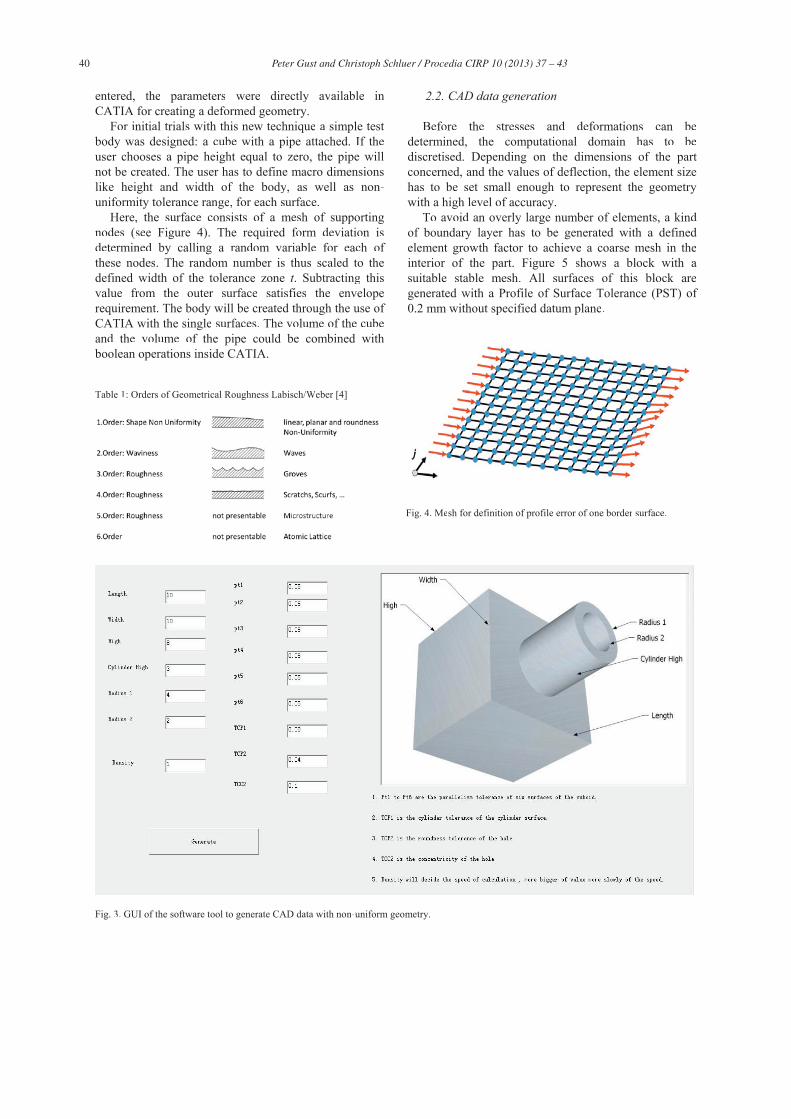
Here, the surface consists of a mesh of supporting nodes (see Figure 4). The required form deviation isdetermined by calling a random variable for each of these nodes. The random number is thus scaled to the defined width of the tolerance zone t. Subtracting thisvalue from the outer surface satisfies the enveloperequirement. The body will be created through the use of CATIA with the single surfaces. The volume of the cubeand the volume of the pipe could be combined withboolean operations inside CATIA.

2.2. CAD data generation

Before the stresses and deformations can be determined, the computational domain has to bediscretised. Depending on the dimensions of the partconcerned, and the values of deflection, the element sizehas to be set small enough to represent the geometry with a high level of accuracy.

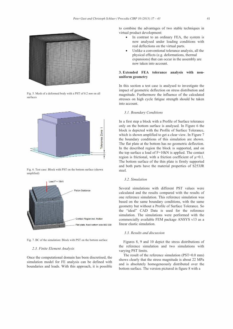
To avoid an overly large number of elements, a kind of boundary layer has to be generated with a defined element growth factor to achieve a coarse mesh in the interior of the part. Figure 5 shows a block with a suitable stable mesh. All surfaces of this block aregenerated with a Profile of Surface Tolerance (PST) of 0.2 mm without specified datum plane.

Table 1: Orders of Geometrical Roughness Labisch/Weber [4]

Fig. 3. GUI of the software tool to generate CAD data with non-uniform geometry.

Fig. 4. Mesh for definition of profile error of one border surface.

41 Peter Gust and Christoph Schluer / Procedia CIRP 10 ( 2013 ) 37 – 43

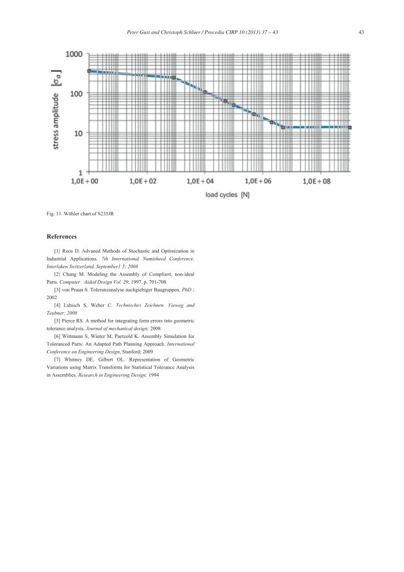
Fig. 7. BC of the simulation: Block with PST on the bottom surface

2.3. Finite Element Analysis

Once the computational domain has been discretised, the simulation model for FE analysis can be defined with boundaries and loads. With this approach, it is possible

to combine the advantages of two stable techniques in virtual product development:

In contrast to an ordinary FEA, the system is now analysed under loading conditions with real deflections on the virtual parts.

Unlike a conventional tolerance analysis, all the physical effects (e.g. deformations, thermal expansions) that can occur in the assembly are now taken into account.

3. Extended FEA tolerance analysis with non-uniform geometry

In this section a test case is analysed to investigate the impact of geometric deflection on stress distribution and magnitude. Furthermore the influence of the calculated stresses on high cycle fatigue strength should be taken into account.

3.1. Boundary Conditions

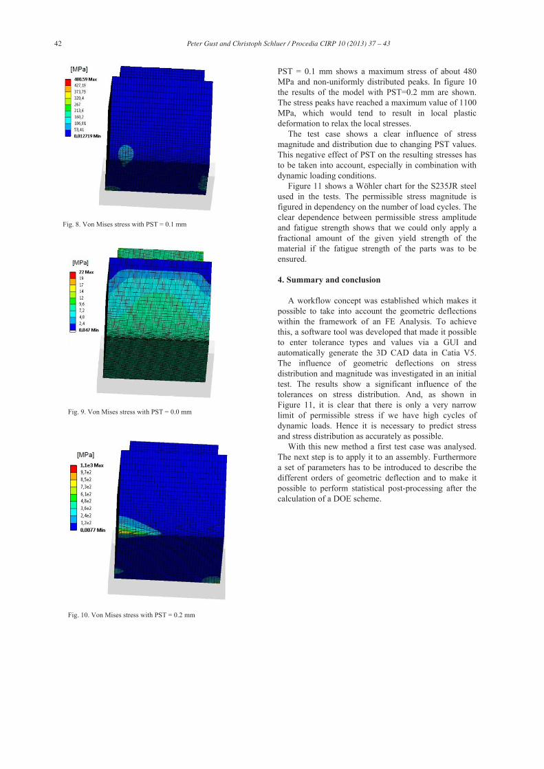
In a first step a block with a Profile of Surface tolerance only on the bottom surface is analysed. In Figure 6 the block is depicted with the Profile of Surface Tolerance, which is shown amplified to get a clear view. In Figure 7 the boundary conditions of this simulation are shown. The flat plate at the bottom has no geometric deflection. In the described region the block is supported, and on the top surface a load of F=10kN is applied. The contact region is frictional, with a friction coefficient of μ=0.1. The bottom surface of the thin plate is firmly supported and both parts have the material properties of S253JR steel.

3.2. Simulation

Several simulations with different PST values were calculated and the results compared with the results of one reference simulation. This reference simulation was based on the same boundary conditions, with the same geometry but without a Profile of Surface Tolerance. So the “ideal” CAD Data is used for the reference simulation. The simulations were performed with the commercially available FEM package ANSYS v13 as a linear elastic simulation.

3.3. Results and discussion

Figures 8, 9 and 10 depict the stress distributions of the reference simulation and two simulations with varying PST limits.

The result of the reference simulation (PST=0.0 mm) shows clearly that the stress magnitude is about 22 MPa and is absolutely homogeneously distributed over the bottom surface. The version pictured in figure 8 with a

Fig. 5. Mesh of a deformed body with a PST of 0.2 mm on all surfaces

Fig. 6. Test case: Block with PST on the bottom surface (shown amplified)

42 Peter Gust and Christoph Schluer / Procedia CIRP 10 ( 2013 ) 37 – 43

PST = 0.1 mm shows a maximum stress of about 480 MPa and non-uniformly distributed peaks. In figure 10 the results of the model with PST=0.2 mm are shown. The stress peaks have reached a maximum value of 1100 MPa, which would tend to result in local plastic deformation to relax the local stresses.

The test case shows a clear influence of stress magnitude and distribution due to changing PST values. This negative effect of PST on the resulting stresses has to be taken into account, especially in combination with dynamic loading conditions.

Figure 11 shows a Wöhler chart for the S235JR steel used in the tests. The permissible stress magnitude is figured in dependency on the number of load cycles. The clear dependence between permissible stress amplitude and fatigue strength shows that we could only apply a fractional amount of the given yield strength of the material if the fatigue strength of the parts was to be ensured.

4. Summary and conclusion

A workflow concept was established which makes it possible to take into account the geometric deflections within the framework of an FE Analysis. To achieve this, a software tool was developed that made it possible to enter tolerance types and values via a GUI and automatically generate the 3D CAD data in Catia V5. The influence of geometric deflections on stress distribution and magnitude was investigated in an initial test. The results show a significant influence of the tolerances on stress distribution. And, as shown in Figure 11, it is clear that there is only a very narrow limit of permissible stress if we have high cycles of dynamic loads. Hence it is necessary to predict stress and stress distribution as accurately as possible.

With this new method a first test case was analysed. The next step is to apply it to an assembly. Furthermore a set of parameters has to be introduced to describe the different orders of geometric deflection and to make it possible to perform statistical post-processing after the calculation of a DOE scheme.

Fig. 8. Von Mises stress with PST = 0.1 mm

Fig. 9. Von Mises stress with PST = 0.0 mm

Fig. 10. Von Mises stress with PST = 0.2 mm

43 Peter Gust and Christoph Schluer / Procedia CIRP 10 ( 2013 ) 37 – 43

References

[1] Roos D. Advaned Methods of Stochastic and Optimization inIndustrial Applications. 7th International Numisheed Conference, Interlaken Switzerland, September1-5; 2008

[2] Chang M. Modeling the Assembly of Compliant, non-idealParts. Computer –Aided Design Vol. 29– ; 1997, p. 701-708

[3] von Praun S. Toleranzanalyse nachgiebiger Baugruppen. PhD ; 2002

[4] Labisch S, Weber C. Technisches Zeichnen. Vieweg and Teubner; 2008

[5] Pierce RS. A method for integrating form errors into geometrictolerance analysis. Journal of mechanical design; 2008

[6] Wittmann S, Winter M, Paetzold K. Assembly Simulation for Toleranced Parts: An Adapted Path Planning Approach. International Conference on Engineering Design, Stanford; 2009

[7] Whitney DE, Gilbert OL. Representation of GeometricVariations using Matrix Transforms for Statistical Tolerance Analysisin Assemblies. Research in Engineering Design; 1994

Fig. 11. Wöhler chart of S235JR