Numerical Integration - uni-tuebingen.dekokkotas/Teaching/Num...Table:Newton-Cotes for numerical...

Numerical Integration

November 28, 2017


Newton - Cotes integration formulas

The Newton-Cotes technique for numerical integrations is similar to theone for finding numerical derivatives of functions. That is, we create theinterpolating polynomial of degree Pn(x) for a given function y(x). Theninstead of integrating the function we integrate the polynomial i.e.∫ b

a

y(x)dx →∫ b

a

Pn(x)dx (1)

where (xs = x0 + sh)

Pn(xs) = f0 + s∆f0 +s(s − 1)

2!∆2f0 +

s(s − 1)(s − 2)

3!∆3f0 + ... (2)

The formulas that one can derive depend on the number of terms of theinterpolating polynomial that we will use. The error will be estimate fromthe integration of the error of the interpolating polynomial used, i.e.

E =

∫ b

a

En(xs)dx (3)

where

En(xs) =s(s − 1)(s − 2)...(s − n)

(n + 1)!hn+1f (n+1)(ξ) where ξ ∈ [a, b] (4)

ξ ∈ [a, b].Numerical Integration

1st order interpolating polynomial

If we use a 1st order interpolating polynomial we get:∫ x1

x0

f (x)dx →∫ x1

x0

P1(xs)dx =

∫ x1

x0

(f0 + s∆f0) dx = h

∫ s=1

s=0

(f0 + s∆f0) ds

= [hf0s]10 +

[h∆f0

s2

2

]10

= h

(f0 +

1

2∆f0

)=

h

2(f0 + f1) (5)

The error introduced when a 1st order polynomial is used is:

f (x)− P(x) =1

2s(s − 1)h2f ′′(ξ) for x0 ≤ ξ ≤ x1 (6)

Then the error in the relation for numerical integration will be estimatedby integrating the above relation

E =

∫ x1

x0

1

2s(s − 1)h2f ′′(ξ)dx =

h3

2

∫ s=1

s=0

s(s − 1)f ′′(ξ)ds

= h3f ′′(ξ1)

(s3

6− s2

4

)1

0

= − 1

12h3f ′′(ξ1) where ξ1 ∈ [x0, x1](7)


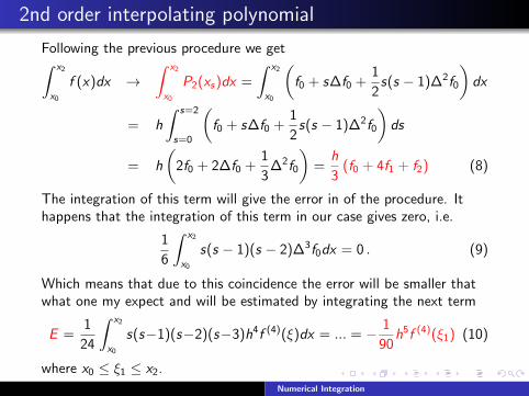
2nd order interpolating polynomial

Following the previous procedure we get∫ x2

x0

f (x)dx →∫ x2

x0

P2(xs)dx =

∫ x2

x0

(f0 + s∆f0 +

1

2s(s − 1)∆2f0

)dx

= h

∫ s=2

s=0

(f0 + s∆f0 +

1

2s(s − 1)∆2f0

)ds

= h

(2f0 + 2∆f0 +

1

3∆2f0

)=

h

3(f0 + 4f1 + f2) (8)

The integration of this term will give the error in of the procedure. Ithappens that the integration of this term in our case gives zero, i.e.

1

6

∫ x2

x0

s(s − 1)(s − 2)∆3f0dx = 0 . (9)

Which means that due to this coincidence the error will be smaller thatwhat one my expect and will be estimated by integrating the next term

E =1

24

∫ x2

x0

s(s−1)(s−2)(s−3)h4f (4)(ξ)dx = ... = − 1

90h5f (4)(ξ1) (10)

where x0 ≤ ξ1 ≤ x2.


3rd order interpolating polynomial

Following the previous procedure we get∫ x3

x0

f (x)dx →∫ x3

x0

P3(xs)dx =3h

8(f0 + 3f1 + 3f2 + f3) . (11)

In a similar fashion we get the error:

E = − 3

80h5f (4)(ξ1) for x0 ≤ ξ1 ≤ x3 (12)

I.e. the error is O(h5) which is of the same order as the error foundearlier by using an interpolating polynomial of 2nd order.

This ”coincidence” in the order of the errors happens also for 4th and 5thorder interpolating polynomials which give an error of the order of O(h7).


Newton – Cotes Formulae

∫ x1

x0

f (x)dx =h

2(f0 + f1)− 1

12h3f (2)(ξ1)

∫ x2

x0

f (x)dx =h

3(f0 + 4f1 + f2)− 1

90h5f (4)(ξ1)

∫ x3

x0

f (x)dx =3h

8(f0 + 3f1 + 3f2 + f3)− 3

80h5f (4)(ξ1)

Table: Newton-Cotes for numerical integration by using 1st, 2nd and 3rdorder interpolating polynomials


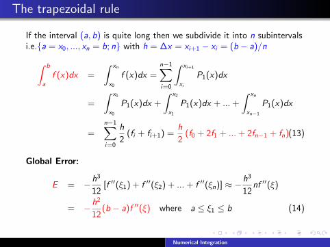
The trapezoidal rule

If the interval (a, b) is quite long then we subdivide it into n subintervalsi.e.{a = x0, ..., xn = b; n} with h = ∆x = xi+1 − xi = (b − a)/n∫ b

a

f (x)dx =

∫ xn

x0

f (x)dx =n−1∑i=0

∫ xi+1

xi

P1(x)dx

=

∫ x1

x0

P1(x)dx +

∫ x2

x1

P1(x)dx + ...+

∫ xn

xn−1

P1(x)dx

=n−1∑i=0

h

2(fi + fi+1) =

h

2(f0 + 2f1 + ...+ 2fn−1 + fn)(13)

Global Error:

E = −h3

12[f ′′(ξ1) + f ′′(ξ2) + ...+ f ′′(ξn)] ≈ −h3

12nf ′′(ξ)

= −h2

12(b − a)f ′′(ξ) where a ≤ ξ1 ≤ b (14)


Simpson’s rules

Simpson’s 1/3 rule∫ b=xn

a=x0

f (x)dx =n−2∑i=0

∫ xi+2

xi

P2(x)dx =n−2∑i=0

h

3(fi + 4fi+1 + fi+2)

=h

3(f1 + 4f2 + 2f3 + 4f4 + ...+ 2fn−2 + 4fn−1 + fn) .(15)

Global Error:

E = −h5

90

n

2f (4)(ξ) = −b − a

180h4f (4)(ξ) for a ≤ ξ ≤ b (16)

Simpson’s 3/8 rule∫ b=xn

a=x0

f (x) dx =3h

8(f0 + 3f1 + 3f2 + 2f3 + ...+ 2fn−3 + 3fn−2 + 3fn−1 + fn)

(17)Global Error:

E = −b − a

80h4f (4)(ξ1) for a ≤ ξ1 ≤ b (18)


Formulas for integration

∫ xn

x0

f (x)dx =h

2(f0 + 2f1 + 2f2 + ...+ 2fn−1 + fn)

− b − a

12h2f (2)(ξ1)∫ xn

x0

f (x)dx =h

3(f0 + 4f1 + 2f2 + 4f3 + ....+ 2fn−2 + 4fn + fn+1)

− b − a

180h4f (4)(ξ1) requires an even number of panels∫ xn

x0

f (x)dx =3h

8(f0 + 3f1 + 3f2 + 2f3 + 3f4 + ....+ 3fn−2 + 3fn−1 + fn)

− b − a

80h4f (4)(ξ1) requires a number of panels divisible by 3

where x0 ≤ ξ1 ≤ xn


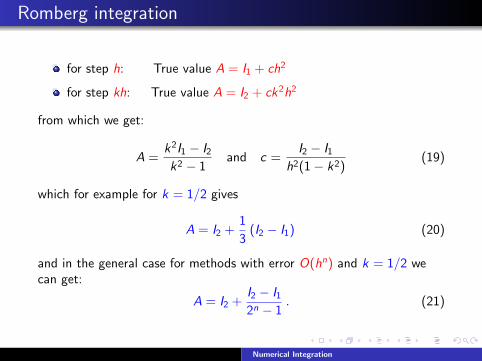
Romberg integration

for step h: True value A = I1 + ch2

for step kh: True value A = I2 + ck2h2

from which we get:

A =k2I1 − I2k2 − 1

and c =I2 − I1

h2(1− k2)(19)

which for example for k = 1/2 gives

A = I2 +1

3(I2 − I1) (20)

and in the general case for methods with error O(hn) and k = 1/2 wecan get:

A = I2 +I2 − I12n − 1

. (21)


Romberg integration : Application

If we start with the trapezoidal rule

I1 =2h

2(f0 + f2) = h (f0 + f2)

I2 =h

2(f0 + f1) +

h

2(f1 + f2) =

h

2(f0 + 2f1 + f2)

then the true value, according to (20), will be

A =2h(f0 + 2f1 + f2)− h(f0 + f2)

3=

h

3(f0 + 4f1 + f2) !!!

EXERCISE: Test numerically the Romberg method for the Simpson 1/3formula.


Splines and integration

For every interval [xi , xi+1] we will have a 3rd order polynomial i.e.

∫ xn

x0

f (x)dx =

n−1∑i=0

[ai

4(x − xi )

4 +bi

3(x − xi )

3 +ci

2(x − xi )

2 + di (x − xi )

]xi+1

xi

=

n−1∑i=0

[ai

4(xi+1 − xi )

4 +bi

3(xi+1 − xi )

3 +ci

2(xi+1 − xi )

2 + di (xi+1 − xi )

].

∫ xn

x0

f (x)dx =h4

4

n−1∑i=0

ai +h3

3

n−1∑i=0

bi +h2

2

n−1∑i=0

ci + hn−1∑i=0

di (22)


Gaussian Quadrature

Mean value theorem:∫ b

a

f (x) dx = (b − a) f (ξ) (23)

We can get an approximate value for the integral by writting

I =

∫ b

a

f (x)dx ≡ c0f (a) + c1f (b) (24)

This will be exact for polynomials of the form f (x) = 1 and f (x) = x

f (x) = x ⇒∫ b

a

x · dx =x2

2

∣∣∣∣ba

=1

2

(b2 − a2

)≡ c0 · a + c1 · b(25)

f (x) = 1 ⇒∫ b

a

1 · dx = x |ba = (b − a) ≡ c0 · 1 + c1 · 1 (26)

c0 =b − a

2and c1 =

b − a

2(27)

Thus ∫ b

a

f (x)dx ≡ b − a

2[f (a) + f (b)] (28)


If we continue by creating according to (24), an relation with 3 terms weget: ∫ b

a

f (x)dx ≡ c0f (a) + c1f

(a + b

2

)+ c2f (b) (29)

This will be exact for polynomials of the form f (x) = 1, f (x) = x andf (x) = x2 and we can get:∫ b

a

f (x)dx =b − a

6

[f (a) + 4f

(a + b

2

)+ f (b)

](30)

This procedure can be extended by using the derivatives i.e.∫ b

a

f (x)dx = c0f (a) + c1f (b) + c2f′(a) + c3f

′(b) (31)

which can be generalized to the Euler-Maclaurin formula∫ xn

x0

f (x) dx =h

2[f (x0) + 2f (x1) + ...+ 2f (xn−1) + f (xn)]

− h2

12[f ′(xn)− f ′(x0)] +

h4

720

[f (3)(xn)− f (3)(x0)

]− h6

30240

[f (5)(xn)− f (5)(x0)

](32)


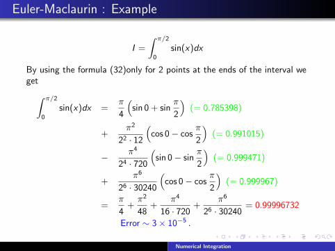
Euler-Maclaurin : Example

I =

∫ π/2

0

sin(x)dx

By using the formula (32)only for 2 points at the ends of the interval weget∫ π/2

0

sin(x)dx =π

4

(sin 0 + sin

π

2

)(= 0.785398)

+π2

22 · 12

(cos 0− cos

π

2

)(= 0.991015)

− π4

24 · 720

(sin 0− sin

π

2

)(= 0.999471)

+π6

26 · 30240

(cos 0− cos

π

2

)(= 0.999967)

=π

4+π2

48+

π4

16 · 720+

π6

26 · 30240= 0.99996732

Error ∼ 3× 10−5 .


Filon’s method

For integral of the type∫ b

a

f (x) sin(x)dx and

∫ b

a

f (x) cos(x)dx

we can try ∫ 2π

0

f (x) sin(x)dx ≈ A1f (0) + A2f (π) + A3f (2π)

which will be true for f (x) = 1, f (x) = x and f (x) = x2

f (x) = 1 ⇒ 0 = A1 + A2 + A3

f (x) = x ⇒ −2π = πA2 + 2πA3

f (x) = x2 ⇒ −4π2 = π2A2 + 4π2A3

with solution A1 = 1, A2 = 0 and A3 = −1.Thus∫ 2π

0

f (x) sin xdx ≈ f (0)− f (2π) .


Filon’s method : General formula

∫ b

a

y(x) sin(kx)dx ≈ h [Ay(a) cos(ka)− Ay(b) cos(kb) + BSe + DSo ] (33)∫ b

a

y(x) cos(kx)dx ≈ h [Ay(a) cos(ka)− Ay(b) cos(kb) + BCe + DCo ] (34)

A =1

q+

sin(2q)

2q2− 2 sin2(q)

q3(35)

B =1

q2+

cos2(q)

q2− sin(2q)

q3(36)

D =4 sin(q)

q3− 4 cos(q)

q2(37)

Se = −y(a) sin(ka)− y(b) sin(kb) + 2n∑

i=0

y(a + 2ih) sin(ka + 2iq)(38)

So =n∑

i=1

y [a + (2i − 1)h] sin [ka + (2i − 1)q] (39)

Ce = −y(a) sin(ka)− y(b) sin(kb) + 2n∑

i=0

y(a + 2ih) sin(ka + 2iq)(40)

Co =n∑

i=1

y [a + (2i − 1)h] sin [ka + (2i − 1)q] (41)

???? q = kh.


Filon’s method : Example

I =

∫ 2π

0

e−x/2 cos(100x)dx = 4.783810813× 10−5 (42)

Notice that Filon’s method with only 4 points outperforms Simpson’smethod with 1000 points

n Simpson Filon4 1.91733833E+0 4.77229440E-58 -5.73192992E-2 4.72338540E-516 2.42801799E-2 4.72338540E-5128 5.55127202E-4 4.78308678E-5256 -1.30263888E-4 4.78404787E-51024 4.77161559E-5 4.78381120E-52048 4.78309107E-5 4.78381084E-5


Gauss’ method

It is an extension of the previous techniques but instead of fixing thepoints of the interval we calculate them together with the weightingcoefficients. For example∫ 1

−1f (x)dx ≈ af (x1) + bf (x2) (43)

this integral can be exact for f (x) = 1, f (x) = x , f (x) = x2 andf (x) = x3. Thus we get the following system of equations:

f (x) = 1 ⇒ 2 = a + bf (x) = x ⇒ 0 = ax1 + bx2f (x) = x2 ⇒ 2

3= ax21 + bx22

f (x) = x3 ⇒ 0 = ax31 + bx32

⇒a = b = 1

x1 = −x2 = −(

13

)1/2= −0.5773∫ 1

−1f (x)dx ≈ f (−0.5773) + f (0.5773)

Thus we need to evaluate the function only at only 2 appropriate pointswhich are: x1 = −0.5773 and x2 = 0.5773.For arbitrary end-points we use the transformation:

t =1

2(b − a)x +

1

2(b + a) and dt =

b − a

2dx . (44)


Gauss’ method : Example

I =

∫ π/2

0

sin(x)dx

We change the variable of integration to get the limits of integration -1and 1

x =1

2

(π2t +

π

2

)=π

4(t + 1) and dx =

π

4dt

and the new integral is:

I =π

4

∫ 1

−1sin[π

4(t + 1)

]dt

=π

4[1.0× sin (0.10566× π) + 1.0× sin (0.39434× π)]

= 0.99849

i.e. an error 1.53× 10−3 while the 2 point trapezoidal rule givesI = 0.7854 and Simposn’s 3 point formula 1.0023.


Gauss-Legendre method

It is a generalization of Gauss’ method of n points, i.e. if∫ 1

−1f (x)dx ≈

n∑i=1

Ai f (xi ) (45)

we have to solve a system of 2n equations to calculate the 2n quantitiesA and xi . This method will be exact for polynomials up to degree2(n − 1) thus the 2n equations can be written as:

A1xk1 + ....+ Anx

kn =

0 for k = 1, 3, 5, ..., 2n − 1

2k+1 for k = 2, 4, 6, ..., 2n − 2

(46)

It can be proved that the xi are roots of the Legendre polynomial of nth-degree which can be always found in the interval (−1, 1). The Legendrepolynomials can be derived from the recursion relation

(n + 1) Ln+1 (x)− (2n + 1) xLn (x) + nLn−1 (x) = 0 (47)

where the first 3 are:

L0 (x) = 1, L1 (x) = x and L2 (x) =3

2x2 − 1

2(48)


Then the Ai are estimated from:

Ai =2(1− x2

)n2 [Ln−1 (xi )]2

(49)

For example, if n = 4 we should find the roots of 4th-degree Legendrepolynomial

P4 =1

8

(35x4 − 30x2 + 3

)which are xi = ±

[(15± 2

√30)/35

]1/2and then by using (49) to

calculate Ai . The exact values are given in the Table 2

n xi Ai

2 ± 0.5773502692 1.0000000004 ± 0.8611363116 0.3478548451

± 0.3394810436 0.65214515498 ± 0.9602898565 0.1012285363

± 0.7966664774 0.2223810345± 0.5255324099 0.3137066459± 0.1834346425 0.3626837834

Table: The values of xi and Ai for the Gauss-Legendre for 2, 4 and 8points.


Generalization of Gauss’s method

For integrals of the type

I =

∫ b

a

w(x)y(x)dx (50)

one can uses alternative orthogonal polynomials, and by writing∫ b

a

w(x)y(x)dx =n∑

i=1

Aiy(xi ) (51)

the unknowns xi and Ai can be found from tables in mathematicalhandbooks. Depending on the form of the weighting function w(x) wehave the following choices:

Gauss-Legendre method for weighting function w(x) = 1.

Gauss-Laguerre method for integrals of the form∞∫0

e−xy (x) dx ≈n∑

i=1

Aiy (xi ) (52)

with weighting function w(x) = e−x where xi are roots of theLaguerre polynomials which can be created from the recursion:


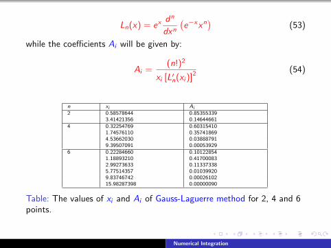
Ln(x) = exdn

dxn(e−xxn

)(53)

while the coefficients Ai will be given by:

Ai =(n!)2

xi [L′n(xi )]2(54)

n xi Ai2 0.58578644 0.85355339

3.41421356 0.146446614 0.32254769 0.60315410

1.74576110 0.357418694.53662030 0.038887919.39507091 0.00053929

6 0.22284660 0.101228541.18893210 0.417000832.99273633 0.113373385.77514357 0.010399209.83746742 0.0002610215.98287398 0.00000090

Table: The values of xi and Ai of Gauss-Laguerre method for 2, 4 and 6points.


• Gauss-Hermite method for integrals of the form∫ ∞−∞

e−x2

y(x)dx ≈n∑

i=1

Aiy(xi ) (55)

i.e. the weighting function is w(x) = e−x2

while the xi are roots of theHermite polynomials. The Hermite polynomials can be created via therelation

Hn(x) = (−1)nex2 dn

dxn

(e−x

2)

(56)

while the coefficients Ai can be found by the relation:

Ai =2n+1n!

√π

[H ′n(xi )]2(57)

Both xi and Ai are given in Table 4.


n xi Ai

2 ± 0.70710678 0.886226934 ± 0.52464762 0.80491409

± 1.65068012 0.081312846 ± 0.43607741 0.72462960

± 1.33584907 0.15706732± 2.35060497 0.00453001

Table: The values xi and Ai of the Gauss-Hermite method for 2, 4 and 6points.


• Gauss-Chebyshev method for integrals of the form:∫ 1

−1

y(x)√1− x2

dx ≈ π

n

n∑i=1

y(xi ) (58)

i.e. the weighting function is

w(x) =1√

1− x2(59)

while the xi are the roots of the Chebyshev polynomials

Tn(x) = cos [n arccos(x)] (60)

and given by the relations

xi = cos[ π

2n(2i − 1)

]. (61)

While the Ai are given by

Ai =π

n(62)

where n is the degree of the polynomial that we use.


Improper and Indefinite integrals

For example:

I =

∫ ∞0

xe−xdx

this can be written as

I =

∫ 1

0

xe−xdx +

∫ ∞1

xe−xdx

and substitute y = 1/x in the 2nd partBut in general we can write it in the form

I = limA→∞

∫ A

0

xe−xdx

and try various values for A. For example

A I1 0.2642410 0.999500600820 0.9999999567157739100 1.00000000∞ 1.0000000


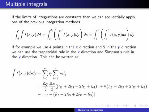
Multiple integrals

If the limits of integrations are constants then we can sequentially applyone of the previous integration methods∫

A

∫f (x , y)dA =

∫ b

a

(∫ d

c

f (x , y)dy

)dx =

∫ d

c

(∫ b

a

f (x , y)dx

)dy

If for example we use 4 points in the x direction and 5 in the y directionwe can use the trapezoidal rule in the x direction and Simpson’s rule inthe y direction. This can be written as:

∫f (x , y)dxdy =

m∑j=1

vj

n∑i=1

wi fij

=∆y

3

∆x

2[(f11 + 2f21 + 2f31 + f41) ] + 4 (f12 + 2f22 + 2f32 + f42)

+ [ · · ·+ (f15 + 2f25 + 2f35 + f45)]


Exercises on Multiple integrals

Try the following example:∫ 1

0

(∫ 2

0

xy2dx

)dy =

2

3∫ 1

0

(∫ 2

2y

xy2dx

)dy =

4

15∫ 2

0

(∫ x/2

0

xy2dy

)dx =?


Numerical Integration - uni-tuebingen.dekokkotas/Teaching/Num...Table:Newton-Cotes for numerical...

Documents

Transcript of Numerical Integration - uni-tuebingen.dekokkotas/Teaching/Num...Table:Newton-Cotes for numerical...