1

Numerical Hydraulics Open channel flow 1

Wolfgang Kinzelbach with

Marc Wolf and

Cornel Beffa

2

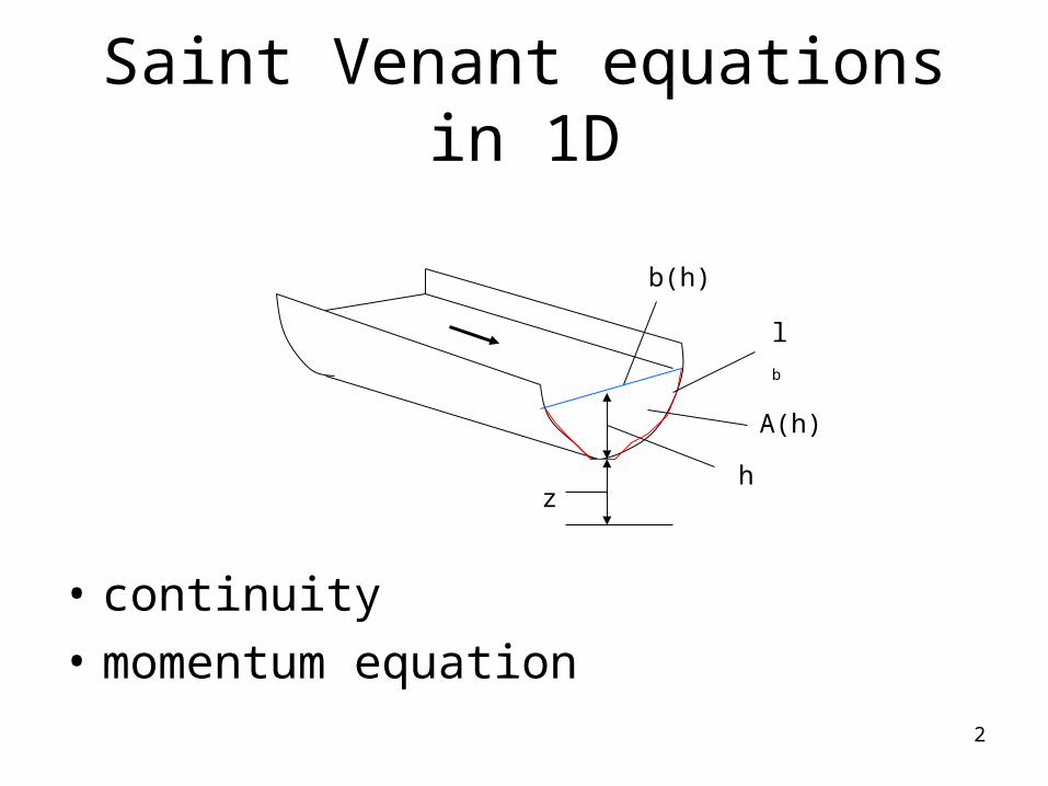
Saint Venant equations in 1D

• continuity

• momentum equation

A(h)

hz

lb

b(h)

3

Saint Venant equations in 1D

• continuity (for section without inflow)

• Momentum equation from integration of Navier-Stokes/Reynolds equations over the channel cross-section:

0Q A

x t

0P

hy

hv vv g

t x x R

4

Saint Venant equations in 1D

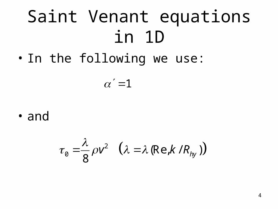
• In the following we use:

• and

20 (Re, / )8 hyv k R

1

5

Saint Venant equations in 1D

The friction can be expressed as energy loss per flow distance:

Using friction slope and channel slope

0 /R

hy

E VgI

R x

21

8R Shy

v zI I

R g x

Alternative: Strickler/Manning equation for IR

6

Saint Venant equations in 1D

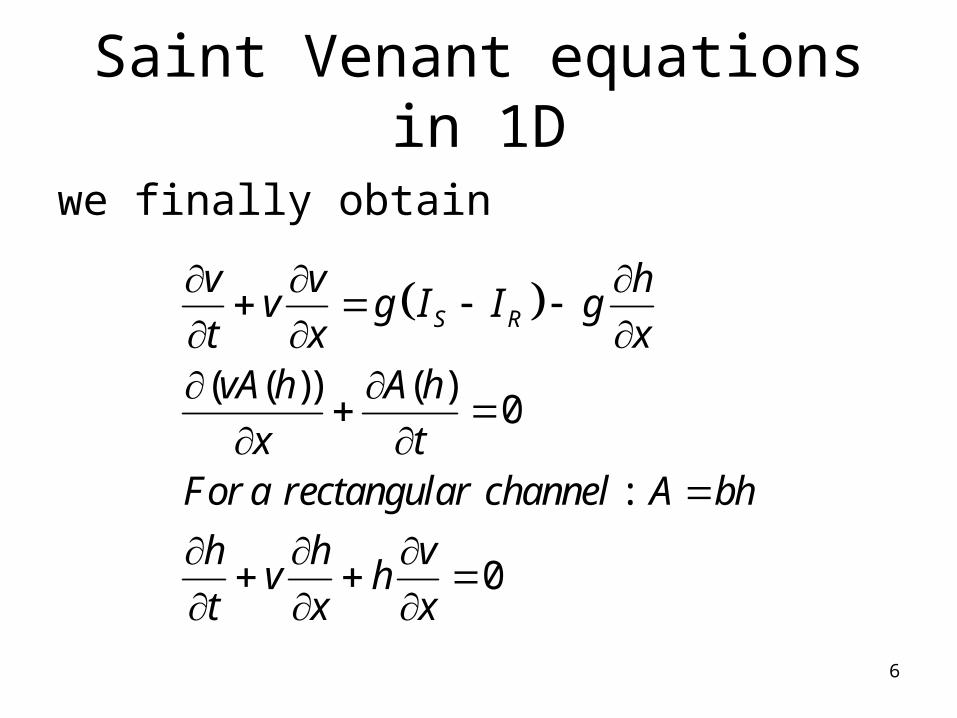
we finally obtain

( ( )) ( )

0

:

0

S R

v v hv g I I g

t x xvA h A h

x tFor a rectangular channel A bh

h h vv h

t x x

7

Approximations and solutions

• Steady state solution

• Kinematic wave

• Diffusive wave

• Full equations

8

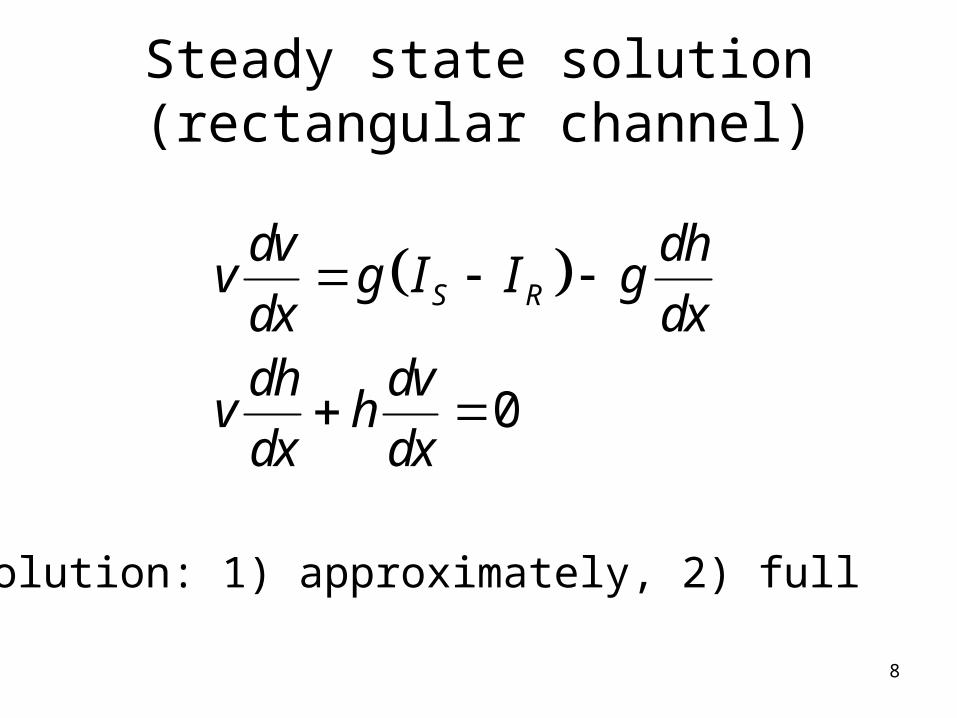
Steady state solution(rectangular channel)

0

S R

dv dhv g I I gdx dxdh dvv hdx dx

Solution: 1) approximately, 2) full

9

Approximation: Neglect advective acceleration

Normal flowFull solution (insert second equation into first):

yields water surface profiles

Steady state solution(rectangular channel)

0S RI I

22

20

1S RI Idh v

with Frdx ghFr

10

Classification of profileshgr = water depth at critical flowhN = water depth at uniform flow

Is = slope of channel bottomIgr = critical slope

Horizontal channel bottomIs = 0

H2: h > hgr

H3: h < hgr

11

Classification of profilesMild slope:

hN > hgr

Is < Igr

M1: hN <h > hgr

M2: hN > h > hgr

M3: hN > h < hgr

Steep slope:hN < hgr

Is > Igr

S1: hN <h > hgr

S2: hN < h < hgr

S3: hN > h < hgr

12

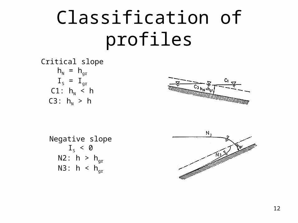
Classification of profiles

Critical slopehN = hgr

IS = Igr

C1: hN < hC3: hN > h

Negative slopeIS < 0

N2: h > hgrgr

N3: h < hgr

13

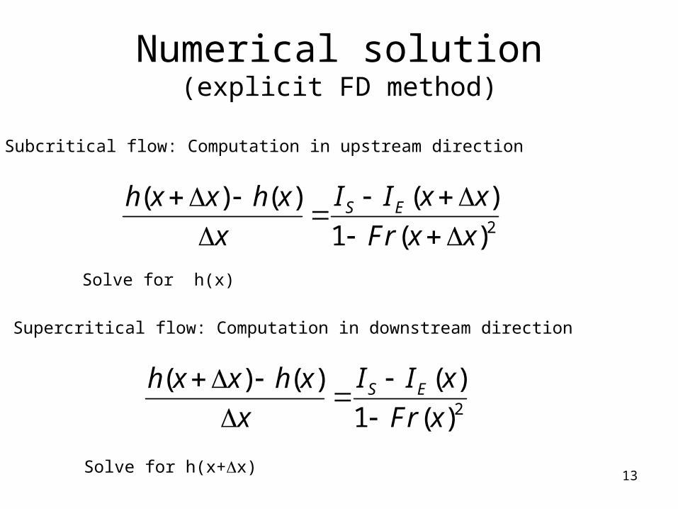
Numerical solution(explicit FD method)

2

( )( ) ( )

1 ( )

S EI I x xh x x h x

x Fr x x

Subcritical flow: Computation in upstream direction

Supercritical flow: Computation in downstream direction

2

( )( ) ( )

1 ( )

S EI I xh x x h x

x Fr x

Solve for h(x)

Solve for h(x+x)