Numerical ElectromagneticsLN08_NTFF [email protected] 1 /19 Near-to-Far-Field Transformation (1...
19
Numerical Electromagnetics LN08_NTFF [email protected] 1 /19 Near-to-Far-Field Transformation (1 Session) (1 Task)
-
Upload
chester-floyd -
Category
Documents
-
view
217 -
download
0
Transcript of Numerical ElectromagneticsLN08_NTFF [email protected] 1 /19 Near-to-Far-Field Transformation (1...
Numerical Electromagnetics LN08_NTFF [email protected] 1 /19
Near-to-Far-Field Transformation
(1 Session)
(1 Task)
Numerical Electromagnetics LN08_NTFF [email protected] 2 /19
Near-to-Far-Field Transformation
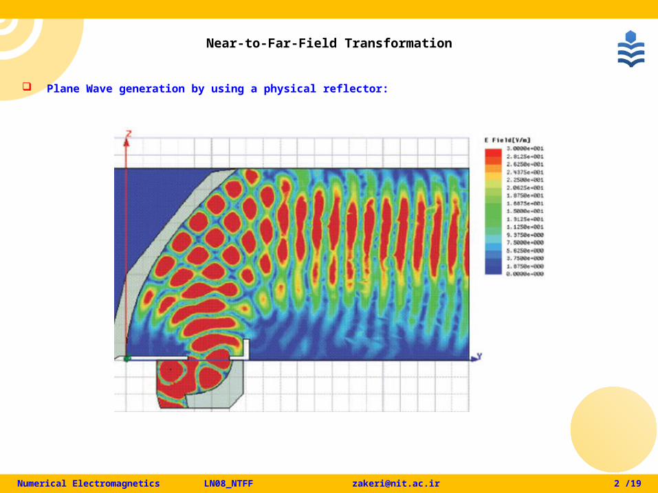
Plane Wave generation by using a physical reflector:

Numerical Electromagnetics LN08_NTFF [email protected] 3 /19
Near-to-Far-Field Transformation
Plane Wave generation by using a non-physical system in FDTD:
TF/SF region in zoned FDTD space lattice, permits a systematic near-to-far-field (NTFF) transformation.
Using near-field data obtained in a single FDTD modeling run, NTFF efficiently and accurately calculates complete far-field bi-static scattering or radiation pattern of an antenna.
There is no need to extend FDTD space lattice to far field.
Using EM Theorem of Surface Equivalent Theory (SET) and using Green's theorem, scattered or radiated fields that are tangential to a closed virtual surface can be integrated to provide far-field response.
Virtual surface is independent of nature of structure being modeled, and can have a fixed rectangular shape to conform with a Cartesian FDTD grid.
This yields powerful SET in two dimensions, which is subsequently extended to general 3D-case.
Resulting analytical NTFF expressions have been implemented in many FDTD codes.
Next, time-domain NTFF transformation, which permits a direct computation of scattered or radiated field-versus-time waveforms, is generated.
Numerical Electromagnetics LN08_NTFF [email protected] 4 /19
Near-to-Far-Field Transformation
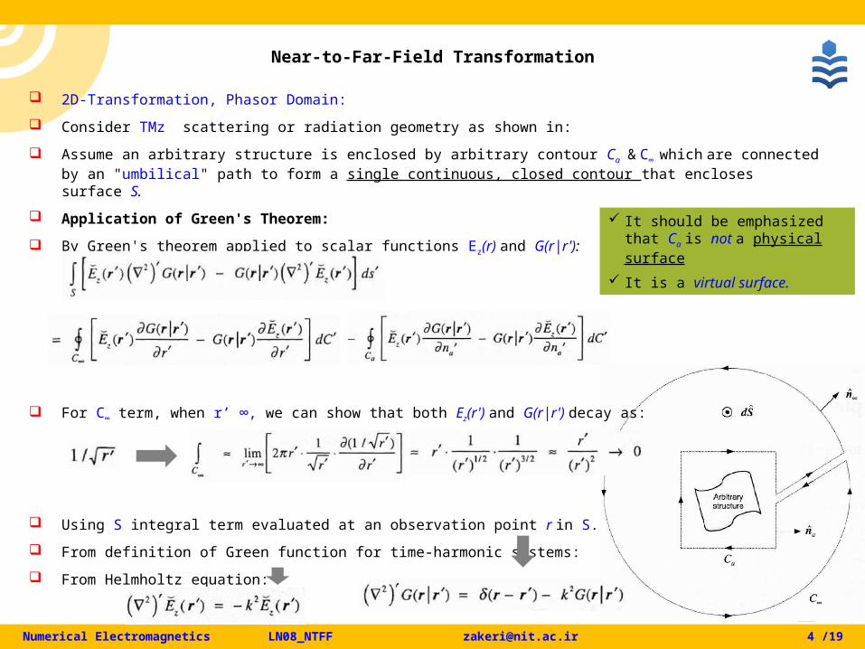
2D-Transformation, Phasor Domain:
Consider TMz scattering or radiation geometry as shown in:
Assume an arbitrary structure is enclosed by arbitrary contour Ca & C∞ which are connected by an "umbilical" path to form a single continuous, closed contour that encloses surface S.
Application of Green's Theorem:
By Green's theorem applied to scalar functions Ez(r) and G(r|r'):
For C∞ term, when r’ ∞, we can show that both Ez(r') and G(r|r') decay as:
Using S integral term evaluated at an observation point r in S.
From definition of Green function for time-harmonic systems:
From Helmholtz equation:
It should be emphasized that Ca is not a physical surface
It is a virtual surface.
Numerical Electromagnetics LN08_NTFF [email protected] 5 /19
Near-to-Far-Field Transformation
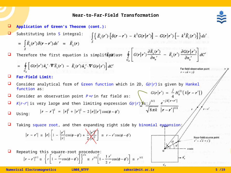
Application of Green's Theorem (cont.):
Substituting into S integral:
Therefore the first equation is simplified as:
Far-Field Limit:
Consider analytical form of Green function which in 2D, G(r|r') is given by Hankel function as:
Consider an observation point P =r in far field as:
K|r-r‘| is very large and then limiting expression G(r|r') is:
Using:
Taking square root, and then expanding right side by binomial expansion:
Repeating this square-root procedure:
Numerical Electromagnetics LN08_NTFF [email protected] 6 /19
Near-to-Far-Field Transformation
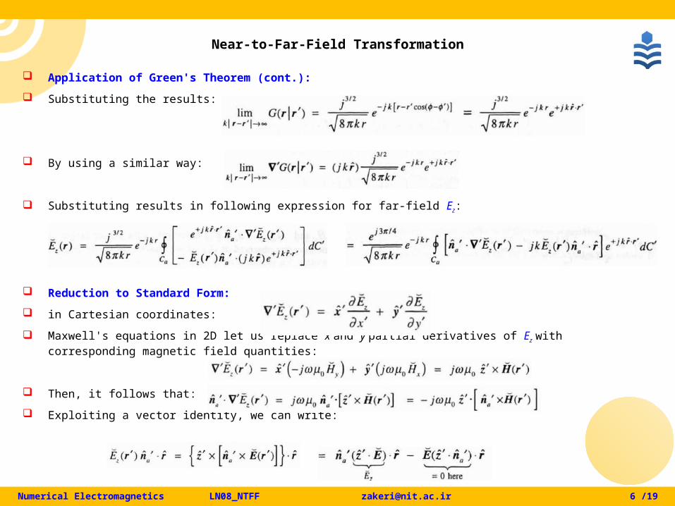
Application of Green's Theorem (cont.):
Substituting the results:
By using a similar way:
Substituting results in following expression for far-field Ez:
Reduction to Standard Form:
in Cartesian coordinates:
Maxwell's equations in 2D let us replace x and y partial derivatives of Ez with corresponding magnetic field quantities:
Then, it follows that:
Exploiting a vector identity, we can write:
Numerical Electromagnetics LN08_NTFF [email protected] 7 /19
Near-to-Far-Field Transformation
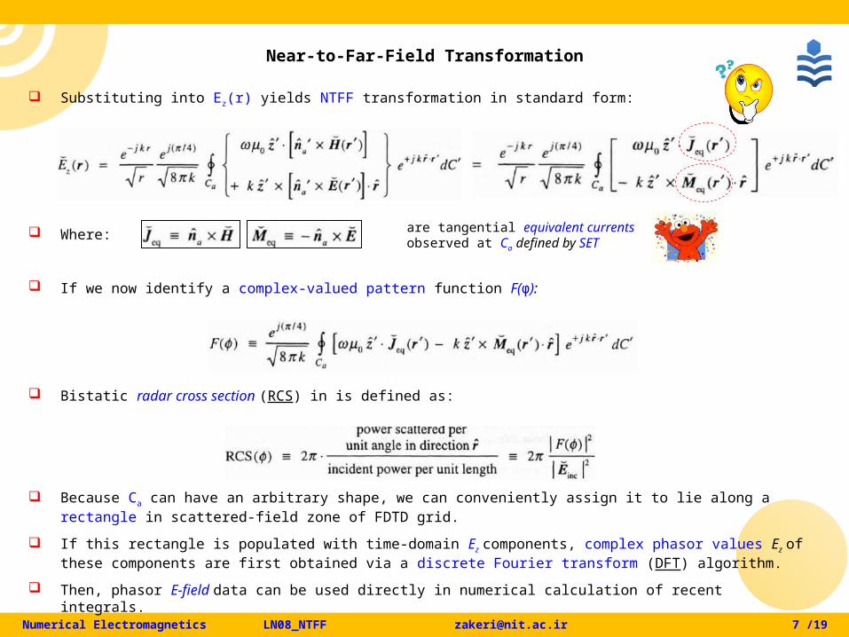
Substituting into Ez(r) yields NTFF transformation in standard form:
Where:
If we now identify a complex-valued pattern function F(φ):
Bistatic radar cross section (RCS) in is defined as:
Because Ca can have an arbitrary shape, we can conveniently assign it to lie along a rectangle in scattered-field zone of FDTD grid.
If this rectangle is populated with time-domain Ez components, complex phasor values Ez of these components are first obtained via a discrete Fourier transform (DFT) algorithm.
Then, phasor E-field data can be used directly in numerical calculation of recent integrals.
are tangential equivalent currents observed at Ca defined by SET
Numerical Electromagnetics LN08_NTFF [email protected] 8 /19
Near-to-Far-Field Transformation
Obtaining Phasor Quantities Via DFT:
Field data used in NTFF transformation are phasor quantities.
At each field point on virtual surface Ca these data can be efficiently and concurrently obtained for multiple frequencies with only one FDTD run.
We need only provide an impulsive wideband electromagnetic excitation of structure of interest, and perform a recursive DFT "on the fly“ (i.e., concurrently with FDTD time-stepping) for each frequency.
Computer storage is quite reasonable, with only two numbers (i.e., the field magnitude and phase) required to store DFT results for each frequency at each field point on virtual surface.
Therefore, a single FDTD run can generate complete far-field distribution of a structure (i.e., its bistatic RCS pattern or its radiation pattern) at many frequencies.
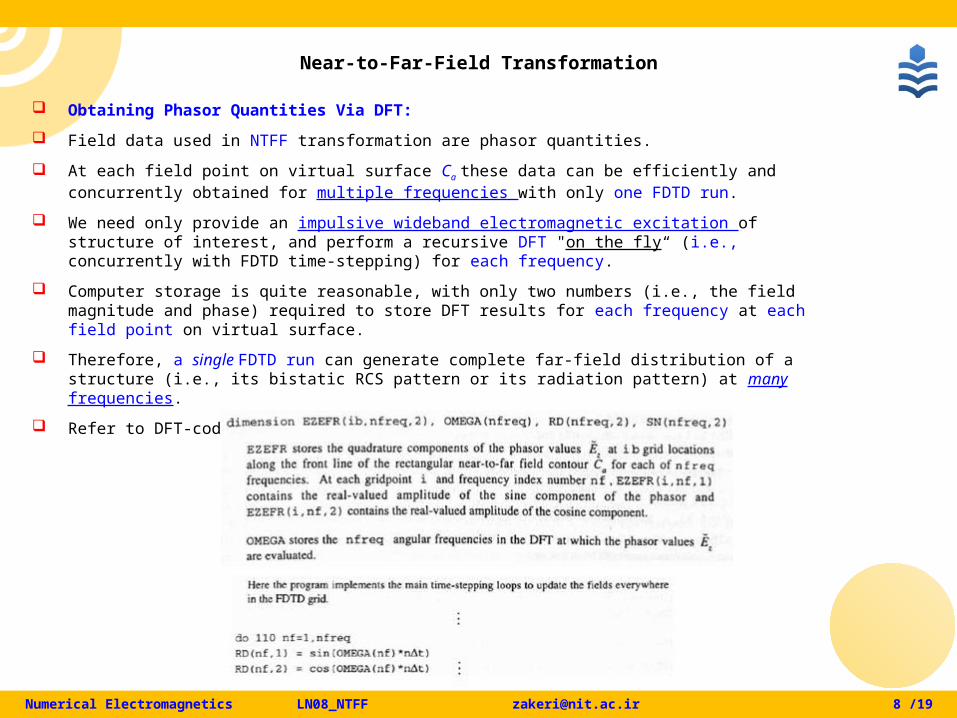
Refer to DFT-code by Fortran in the book as:
Numerical Electromagnetics LN08_NTFF [email protected] 9 /19
Surface Equivalence Theorem
Surface Equivalence Theorem:
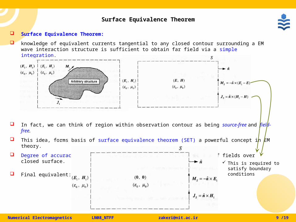
knowledge of equivalent currents tangential to any closed contour surrounding a EM wave interaction structure is sufficient to obtain far field via a simple integration.
In fact, we can think of region within observation contour as being source-free and field-free.
This idea, forms basis of surface equivalence theorem (SET) a powerful concept in EM theory.
Degree of accuracy depends on knowledge of tangential components of fields over closed surface.
Final equivalent:
This is required to satisfy boundary conditions
Numerical Electromagnetics LN08_NTFF [email protected] 10 /19
Extension to 3D-Phasor Domain
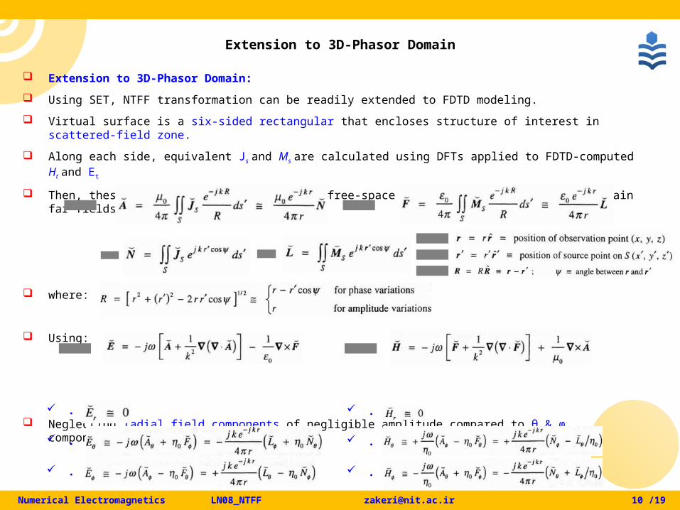
Extension to 3D-Phasor Domain:
Using SET, NTFF transformation can be readily extended to FDTD modeling.
Virtual surface is a six-sided rectangular that encloses structure of interest in scattered-field zone.
Along each side, equivalent Js and Ms are calculated using DFTs applied to FDTD-computed Ht and Et
Then, these currents are integrated with free-space Green function weighting to obtain far-fields:
where:
Using:
Neglecting radial field components of negligible amplitude compared to θ & φ components:
.
.
.
.
.
.
Numerical Electromagnetics LN08_NTFF [email protected] 11 /19
Extension to 3D-Phasor Domain
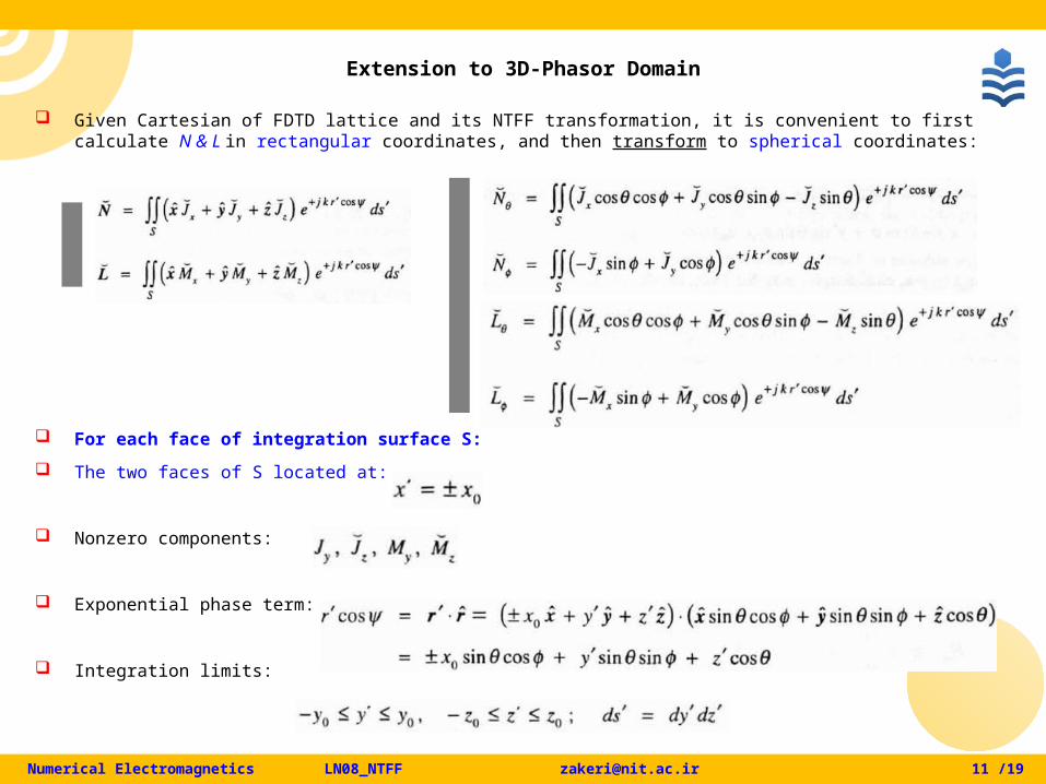
Given Cartesian of FDTD lattice and its NTFF transformation, it is convenient to first calculate N & L in rectangular coordinates, and then transform to spherical coordinates:
For each face of integration surface S:
The two faces of S located at:
Nonzero components:
Exponential phase term:
Integration limits:
Numerical Electromagnetics LN08_NTFF [email protected] 12 /19
Extension to 3D-Phasor Domain
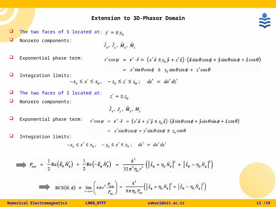
The two faces of S located at:
Nonzero components:
Exponential phase term:
Integration limits:
The two faces of S located at:
Nonzero components:
Exponential phase term:
Integration limits:
Numerical Electromagnetics LN08_NTFF [email protected] 13 /19
Time Domain Near-to-far-field Transformation (TD-NTFF)
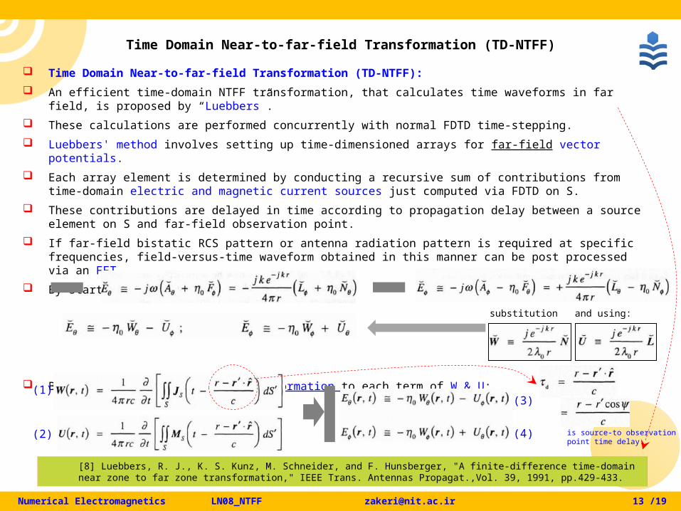
Time Domain Near-to-far-field Transformation (TD-NTFF):
An efficient time-domain NTFF transformation, that calculates time waveforms in far field, is proposed by “Luebbers”.
These calculations are performed concurrently with normal FDTD time-stepping.
Luebbers' method involves setting up time-dimensioned arrays for far-field vector potentials.
Each array element is determined by conducting a recursive sum of contributions from time-domain electric and magnetic current sources just computed via FDTD on S.
These contributions are delayed in time according to propagation delay between a source element on S and far-field observation point.
If far-field bistatic RCS pattern or antenna radiation pattern is required at specific frequencies, field-versus-time waveform obtained in this manner can be post processed via an FFT.
By starting:
By applying inverse Fourier transformation to each term of W & U:
substitution and using:
[8] Luebbers, R. J., K. S. Kunz, M. Schneider, and F. Hunsberger, "A finite-difference time-domain near zone to far zone transformation," IEEE Trans. Antennas Propagat.,Vol. 39, 1991, pp.429-433.
(1)
(2)
(3)
(4) is source-to observation point time delay.

Numerical Electromagnetics LN08_NTFF [email protected] 14 /19
Consider implementation of (1) to (4) in context of FDTD method.
Overall strategy is to evaluate integrals of (1) and (2) in Cartesian coordinates along six planar faces of S at each time-step.
To illustrate core of this process, use example (11) in [8], by using as a sample excitation magnetic current as:
From (1), M yields following additive increment to U(r, t):
This increment contributes to U(r,t) after time delay d, expressed as time-steps:
Assuming a second-order-accurate central-difference of (5) using FDTD notation:
It is clear that process discussed above can be implemented in an analogous manner for Ux(r,t) and Uy(r,t), as well as for three Cartesian components of Wx(r,t), Wy(r,t) and Wz(r,t).
Time Domain Near-to-far-field Transformation (TD-NTFF)
(5)
𝑧
𝑥Δ𝑥
Δ 𝑧
𝑦
𝑦 0𝑟 ′
virtual surface S
Numerical Electromagnetics LN08_NTFF [email protected] 15 /19
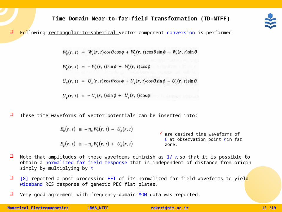
Following rectangular-to-spherical vector component conversion is performed:
These time waveforms of vector potentials can be inserted into:
Note that amplitudes of these waveforms diminish as 1/ r, so that it is possible to obtain a normalized far-field response that is independent of distance from origin simply by multiplying by r.
[8] reported a post processing FFT of its normalized far-field waveforms to yield wideband RCS response of generic PEC flat plates.
Very good agreement with frequency-domain MOM data was reported.
Time Domain Near-to-far-field Transformation (TD-NTFF)
are desired time waveforms of E at observation point r in far zone.
Numerical Electromagnetics LN08_NTFF [email protected] 16 /19
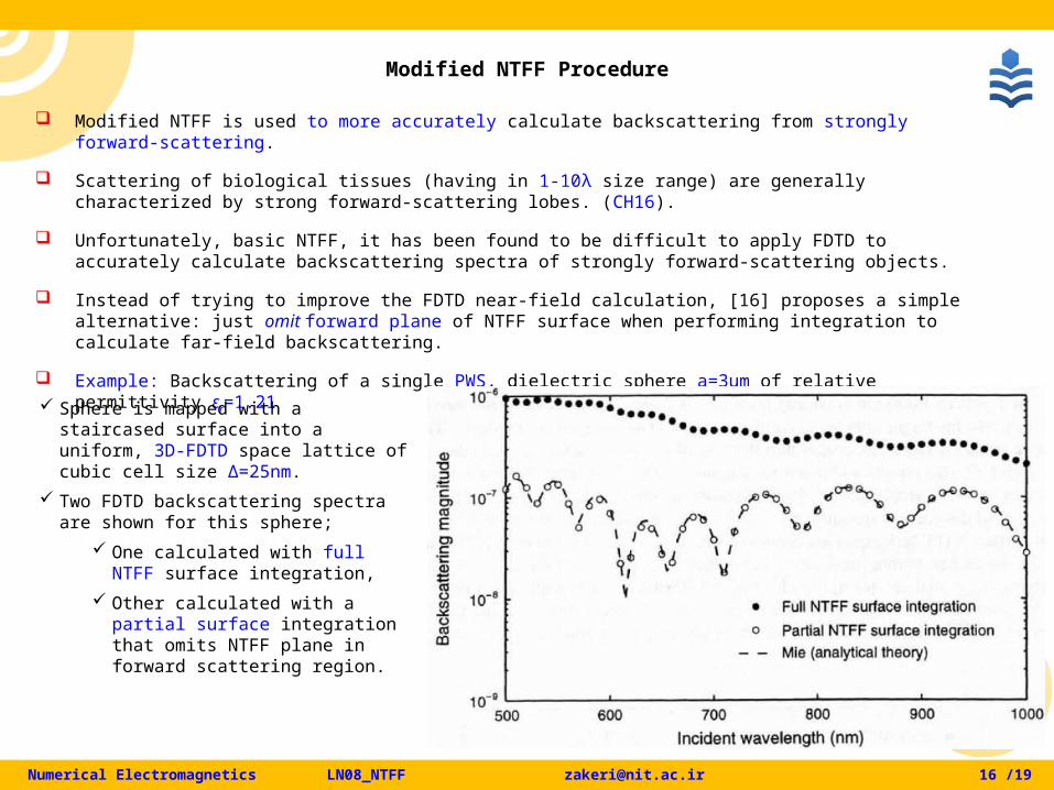
Modified NTFF is used to more accurately calculate backscattering from strongly forward-scattering.
Scattering of biological tissues (having in 1-10λ size range) are generally characterized by strong forward-scattering lobes. (CH16).
Unfortunately, basic NTFF, it has been found to be difficult to apply FDTD to accurately calculate backscattering spectra of strongly forward-scattering objects.
Instead of trying to improve the FDTD near-field calculation, [16] proposes a simple alternative: just omit forward plane of NTFF surface when performing integration to calculate far-field backscattering.
Example: Backscattering of a single PWS, dielectric sphere a=3um of relative permittivity εr=1.21
Modified NTFF Procedure
Sphere is mapped with a staircased surface into a uniform, 3D-FDTD space lattice of cubic cell size Δ=25nm.
Two FDTD backscattering spectra are shown for this sphere;
One calculated with full NTFF surface integration,
Other calculated with a partial surface integration that omits NTFF plane in forward scattering region.
Numerical Electromagnetics LN08_NTFF [email protected] 17 /19
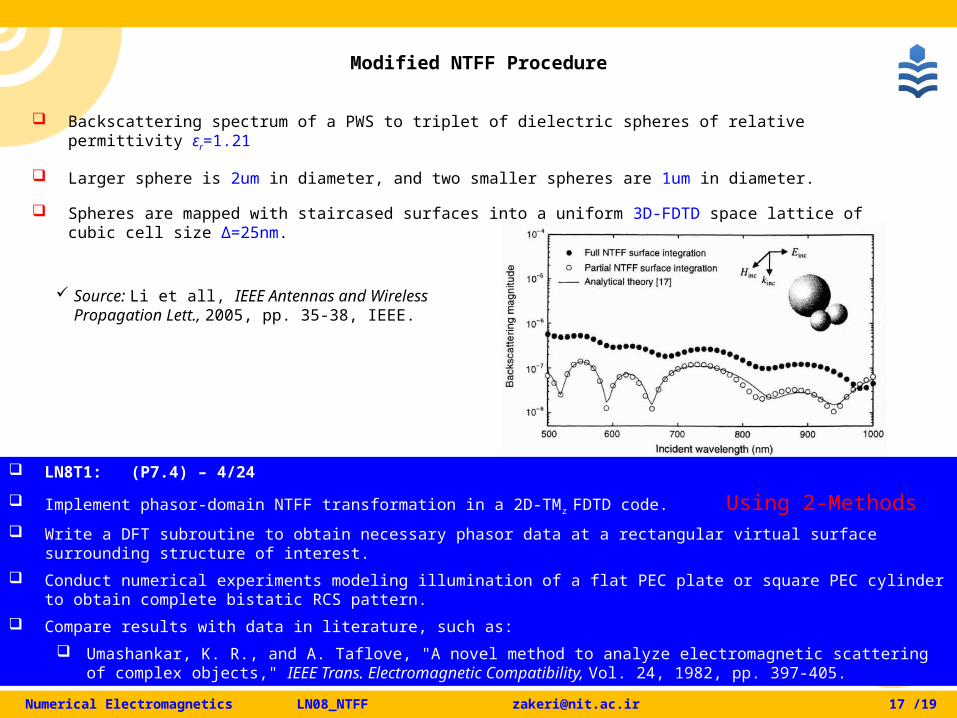
Backscattering spectrum of a PWS to triplet of dielectric spheres of relative permittivity εr=1.21
Larger sphere is 2um in diameter, and two smaller spheres are 1um in diameter.
Spheres are mapped with staircased surfaces into a uniform 3D-FDTD space lattice of cubic cell size Δ=25nm.
Source: Li et all, IEEE Antennas and Wireless Propagation Lett., 2005, pp. 35-38, IEEE.
LN8T1: (P7.4) – 4/24
Implement phasor-domain NTFF transformation in a 2D-TMz FDTD code. Using 2-Methods Write a DFT subroutine to obtain necessary phasor data at a rectangular virtual surface surrounding structure of
interest.
Conduct numerical experiments modeling illumination of a flat PEC plate or square PEC cylinder to obtain complete bistatic RCS pattern.
Compare results with data in literature, such as:
Umashankar, K. R., and A. Taflove, "A novel method to analyze electromagnetic scattering of complex objects," IEEE Trans. Electromagnetic Compatibility, Vol. 24, 1982, pp. 397-405.
Modified NTFF Procedure
Numerical Electromagnetics LN08_NTFF [email protected] 18 /19
Summary & introduced topics:
1. Basis of frequency and time domain NTFF transformations for FDTD simulations is introduced.
2. Using phasor-domain Green's theorem to prove that scattered or radiated fields tangential to a virtual surface enclosing structure being modeled can be integrated to provide complete far-field pattern.
3. virtual surface is independent of shape or composition of structure being modeled.
4. Phasor data needed for this calculation can be efficiently obtained during FDTD run by running a concurrent DFT on time-stepped field components tangential to designated virtual surface in lattice.
5. These discussions motivated a review of a powerful phasor-domain surface equivalence theorem.
6. A numerical implementation is used for a time-domain NTFF transformation which permits direct computation of scattered or radiated pulses at a set of angles in far field.
This procedure can be used instead of phasor-domain transformation discussed earlier, if required data are time waveforms, and there are relatively few far-field observation angles of interest.
7. A recent simple modification of NTFF procedure that greatly improves accuracy in calculating backscatter from strongly forward-scattering objects, such as biological cells illuminated by light and certain types of low-observable vehicles.
8. Modification involves simply omitting forward plane of NTFF surface when performing integration to calculate far-field backscattering.
9. This avoids "subtraction noise“ problem posed by requirement for near cancellation of relatively large field values collected on this plane when integrated into far backscattered field.
Near-to-Far-Field Transformation
Numerical Electromagnetics LN08_NTFF [email protected] 19 /19
Summary on NTFF:
There are two alternatives performing NTFF transformation:
1. On-the-fly (real-time) time-domain transformation that calculates time waveforms of scattered or radiated E-and H-fields at previously specified angular positions in far field. These calculations are performed simultaneously with normal FDTD time-stepping.
2. Frequency-domain transformation that computer transformation of fields in whole far field region at a selected frequency point. First Discrete Fourier Transform (DFT) has to be performed on collected equivalent current densities over virtual surface within FDTD iteration loop. Then based on results near-to-far-field transformation is conducted on specified frequency point.
NTFF transformation alternatives in CADs:
FD near-to-far-field transform:
This transform is useful if the user wants the far-field information at a number of prescribed frequencies. A compensation procedure has been implemented for significantly reduce the dispersion error of the incoming wave.
CW near-to-far-field transform:
For problems where a continuous wave source with a single frequency is used and an efficient continuous wave near-to-far-field transformation can be utilized.
TD near-to-far-field transform:
This transform directly computes the scattered or radiated field versus time during the FDTD time stepping. The frequency domain fields can then be obtained by FFT post-processing.
Near-to-Far-Field Transformation