Numerical coupling of Modelica and CFD for building energy supply systems

Manuel Ljubijankic1 Christoph Nytsch-Geusen1 Jörg Rädler1 Martin Löffler2

1Universität der Künste Berlin, Lehrstuhl für Versorgungsplanung und Versorgungstechnik Hardenbergstraße 33, 10623 Berlin

2TLK-Thermo GmbH, Hans-Sommer-Str. 5, 38106 Braunschweig nytsch@udk-berlin.de m.loeffler @tlk-thermo.de

Abstract

This paper presents an integrated method for the si-mulation of mixed 1D / 3D system models in the domain of building energy supply systems. The fea-sibility of this approach is demonstrated by the use case of a solar thermal system: the sub-model of a hot water storage is modeled as a detailed three-dimensional CFD model, but the rest of the system model (solar collector, hydraulics, heat exchanger, controller etc.) is modeled as a simplified compo-nent-based DAE model. For this purpose, the hot water storage model is simulated with ANSYS CFD. This detailed sub-model is embedded in the solar thermal system model, which consists of component models of the Modelica library FluidFlow and is si-mulated with Dymola. The numerical coupling and integration of both sub-models is realized by the use of the co-simulation environment TISC. With a comparison of a pure Modelica system model and a mixed 1D / 3D system model of the same solar ther-mal system, advantages and disadvantages of both simulation approaches are worked out.

Keywords: Co-simulation; Mixed 1D/3D modeling; energy building and plant simulation

1 Introduction

Up to now, the simplified world of DAE (Diffe-rential Algebraic Equation) system simulation and the detailed world of CFD (Computational Fluid Dynamics) simulation have been two different “modeling cultures” in the domain of building ener-gy supply systems. Users of component based DAE system simulation tools/approaches like Modelica

[1], MATLAB/Simulink [2], TRNSYS [3] analyze the transient behavior of complex energy system models, which include simplified physical sub-models of the energy supply systems, models for the supplied buildings and models for the control algo-rithms of the energy management. Because the com-plexity of these models is reduced (typically some hundred up to 100,000 model variables), the time periods in simulation experiments can be a week, a month or a year.

In comparison to the simplified systems models, detailed 3D CFD models are used to optimized the thermal comfort of a room (e.g. to find suitable posi-tions of inlet and outlet air passages, which guaran-tee comfortable local air temperatures and air veloci-ties) or to optimize the flow conditions and the heat transfer within a building services component (e.g. to design the inner geometry of a heat water storage). The second type of models uses highly discretized Finite Element Models (FEM) ore Finite Volume Models (FVM) with up to several million equations. For this detailed models, the used time period in transient simulation experiments can be - restricted by the currently existing numerical power - some seconds up to some days.

The basic idea of this article is to combine both worlds to a numerical integrated simulation approach for building energy supply systems (compare with Figure 1): the DAE simulation tool (e.g. Dymola) produces with the help of its - component-based - one-dimensional Modelica model transient (“intelli-gent”) boundary conditions for the detailed three-dimensional CFD tool/model and vice versa. In this way, the most interesting part(s) of a system model can be analyzed on a more detailed level, wherein the system relationships are fully taken into account.

Proceedings 8th Modelica Conference, Dresden, Germany, March 20-22, 2011

286

1D-DAE Simulation Tool

Dymola

3D-CFD Simulation Tool

ANSYS CFD

Co-Simulation Environment

TISC

Simplified (component based)system model, based on

the Modelica library FluidFlowfor thermo-hydraulic systems

Detailed (geometric) sub model, based on a continuous flow area

Figure 1: Numerical integrated simulation approach for DAE / CFD modeling of building energy supply systems

The numerical data exchange and the synchroni-zation of the numerical solvers of several simulation tools are realized by the use of the co-simulation en-vironment TISC [12]. In this procedure, it is very important to use “appropriate models” from the DAE- and the CFD-world, this means the models use a comparable physics, and they produce similar re-sults on an aggregated level. Preliminary studies on this have been undertaken by the authors [14, 15].

2 Use case: Solar thermal system

For doing the comparative system simulation studies about the numerical coupling between the DAE-approach of Modelica and the CFD-approach, a solar thermal system for warm water production was used as a reference system (see Figure 2).

solar pump storage pump

solar collector

solar loop

storage loop

controller

heat exchanger

weather

thermal storage

Figure 2: Used solar thermal system for the simula-tion studies

The most important components of the solar thermal system are an evacuated tube collector (type Viess-mann VITOSOL 200 T) with an aperture area of 3.17 m2 and a hot water storage with a volume of 400 liter. The roof collector is aligned to the south

and tilted with an angle of 30°. Here, the vertical distance between the roof and the storage is 10 m. The cylindrical shaped storage has a height of 1.45 m and a diameter of 0.59 m and is isolated with 100 mm insulation (λ = 0.06 W/(m·K)). An external plate heat exchanger (k·A = 1,000 W/K) transfers the pro-duced thermal energy from the solar loop to the sto-rage loop. With the help of a two-point-controller the solar pump and the storage pump are switched on (mass flow rate 0.0264 kg/s), if the collector outlet temperature is 4°K higher than the temperature in the lower part of the storage (hysteresis of 5°K). All hy-draulic components of the solar thermal system are connected with copper pipes with an inside diameter of 26 mm, a wall thickness of 1 mm and an insula-tion thickness of 30 mm (λ = 0.035 W/(m·K). For the climate boundary condition Meteonorm [16] weather data from Hamburg (Germany) were used. In the simulation scenario the load process for the thermal water storage over a time period of 24 h (86,400 seconds) during a summer day were ana-lyzed. At the beginning of the load process all the fluid temperatures in the collector, in all pipes and in the storage shall be 20 °C.

3 System simulation with Modelica

To obtain a reference system for the evaluation of the coupled Modelica/CFD-model, in a first step the solar thermal system was modeled as a pure Modeli-ca model. For this purpose, the FluidFlow-library was used.

3.1 Modelica FluidFlow library

The Modelica-library FluidFlow is being developed at UdK Berlin for thermo-hydraulic network simula-tion [4]. The main application field of this library is the modeling of solar thermal systems, HVAC (Heat-ing, Ventilation and Air-Conditioning)-systems and district heating/cooling systems. The FluidFlow-library comprises a set of “ready-to-use” standard hydraulic models, such as pipes, el-bows, distributors and pumps. Further, the library includes more specialized models from several do-mains (compare with Figure 3), such as solar thermal technologies (collector models), thermal storage technologies (storage models) or energy transforma-tion technologies (e.g. models of heat exchangers, absorption chillers and cogeneration plants). The weather data sets are read and interpolated with a new developed Modelica component, based on the ncDataReader2 library, which provides access to external data sets as continuous functions [5].

Proceedings 8th Modelica Conference, Dresden, Germany, March 20-22, 2011

287

Figure 3: Standard models (left) and specialized models (right) of the thermal-hydraulic Modelica library FluidFlow.

Up to now the main application field of the

FluidFlow-library was the modeling and simulation of complex energy supply systems (heating and cool-ing energy) for new planned city districts with resi-dential buildings in Iran [6].

3.2 Modeling as pure Modelica system model

Figure 4 shows the system model of the solar ther-mal system from the use case, solely modeled with sub-components of the Modelica FluidFlow-library.

Figure 4: Solar thermal system, modeled as system model with pure Modelica sub-components

The used physical models (solar collector, pipes, ex-ternal heat exchanger, hot water storage) were vali-dated from [7]. All the pipes were parameterized in a way that a minimum of 1 numerical node per 1 m pipe length can be ensured. The hot water storage

model is divided into 10 thermal horizontal zones. This modeling approach leads to a system model with 721 time variables. With the symbolic reduction algorithm of the used simulation tool Dymola [8], the DAE-system could be reduced to 419 time vary-ing variables.

In order to define suitable and comparable inter-faces to the Modelica/CFD system model, a sub-system for the hot water storage and its boundary conditions (connection pipes, inlet boundary condi-tions, models for the pressure losses for the flow di-lation and contraction) were introduced (compare with Figure 5).

Figure 5: Modelica sub-system for the thermal sto-rage and its boundary conditions

4 Modelica system simulation with an integrated CFD sub-model

4.1 Modeling and simulation with ANSYS CFD

In order to determine the model state at any point of the volume of the hot water storage (e.g. tempera-tures, velocities, pressures), the three-dimensional CFD method was used. In our case, the fluid region of the hot water storage is modeled with ANSYS CFD Release 12.1 [9], which works with CFD algo-rithms, based on the Finite Volume Method (FVM). The FVM method calculates approximated solutions of the partial differential equation system, which de-scribes the transport process of momentum, mass and

Proceedings 8th Modelica Conference, Dresden, Germany, March 20-22, 2011

288

heat transfer within the flow region (Navier-Stokes equations):

Continuity equation:

∂ρ∂t

+ ∇ • ρ U( )= 0, (1)

Three momentum equations (vector notation with the Nabla-operator for the three Cartesian coordinates):

∂ ρ U( )∂t

+ ∇ • ρ U ⊗ U( )= −∇p + ∇ • τ , (2)

Total energy equation:

∂ ρ htot( )

∂t− ∂p

∂t+ ∇ • ρ U htot( )

= ∇ • λ∇T( )+ ∇ • U•τ( ).

(3)

For each element of the flow region a discretized form of the mentioned 5 partial differential equations is calculated from the ANSYS CFD numerical solver.

4.2 3D CFD model of the hot water storage

An adequate three-dimensional model of the hot wa-ter storage has to fulfill several aspects:

1. The discretization of the fluid regime has to be

fine enough to limit the numerical error. For this purpose, the size of the elements has to be adapted to the local geometries und the local ve-locities.

2. The CFD model has to be fast enough for a coupled transient simulation.

3. The location of the interface planes between the three-dimensional CFD fluid regime and the one-dimensional Modelica fluid regime have to be chosen in a way, that the fluid flow at the in-terface point can take place without a significant disturbance, which can be induced by the inner fluid flow pattern of the storage.

For this reason, the fluid regime of the cylindrical storage was supplemented by two connection pipes with a length of 0.275 m. This necessary length was established by preliminary CFD flow pattern tests with a typical mass flow from the storage pump (0.026 kg/s). The compromise between a needed ac-curacy and a desired numerical performance is a

mesh with all in all 21,904 numerical nodes (85,230 finite volume elements). Hereof 5,440 numerical nodes (5,370 finite volume elements) are used for the connection pipe models and 16,464 numerical nodes (79,860 finite volume elements) for the storage mod-el (compare with Figure 6). The used turbulence model was a laminar model, because the range of values of the Reynolds number of the fluid regime, which can be assigned to the connection pipes, reaches from of 1,290 (20 °C) up to 2,230 (47 °C).

Figure 6: Adapted Mesh of the finite volume storage model: longitudinal section (above), horizontal view on the storage with connection pipe (below left), ho-rizontal sections close to the inlet (below middle) and in the middle of the storage (below right)

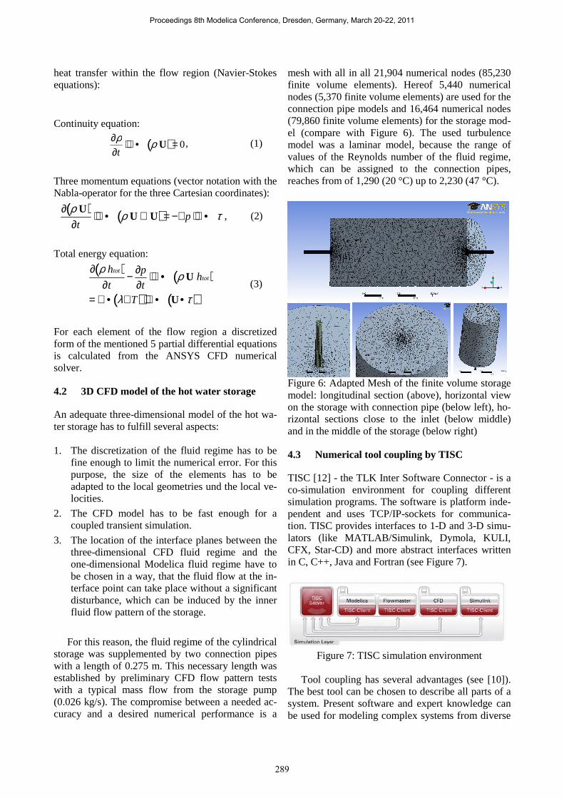
4.3 Numerical tool coupling by TISC

TISC [12] - the TLK Inter Software Connector - is a co-simulation environment for coupling different simulation programs. The software is platform inde-pendent and uses TCP/IP-sockets for communica-tion. TISC provides interfaces to 1-D and 3-D simu-lators (like MATLAB/Simulink, Dymola, KULI, CFX, Star-CD) and more abstract interfaces written in C, C++, Java and Fortran (see Figure 7).

Figure 7: TISC simulation environment

Tool coupling has several advantages (see [10]).

The best tool can be chosen to describe all parts of a system. Present software and expert knowledge can be used for modeling complex systems from diverse

Proceedings 8th Modelica Conference, Dresden, Germany, March 20-22, 2011

289

physical and engineering domains (see [11]). In some cases, it also makes sense to break down a model or system into several sub-systems to de-couple the time steps and accelerate the simulation. Using TISC makes it also possible to integrate tran-sient boundary conditions from different specialized simulation tools. For example, the input and output data from a detailed FEM or CFD simulation tool are available for a DAE Modelica model in Dymola and vice versa. Distributed computation of a system on several cores also provides the opportunity to paral-lelize a simulation calculation and get more compu-tation performance.

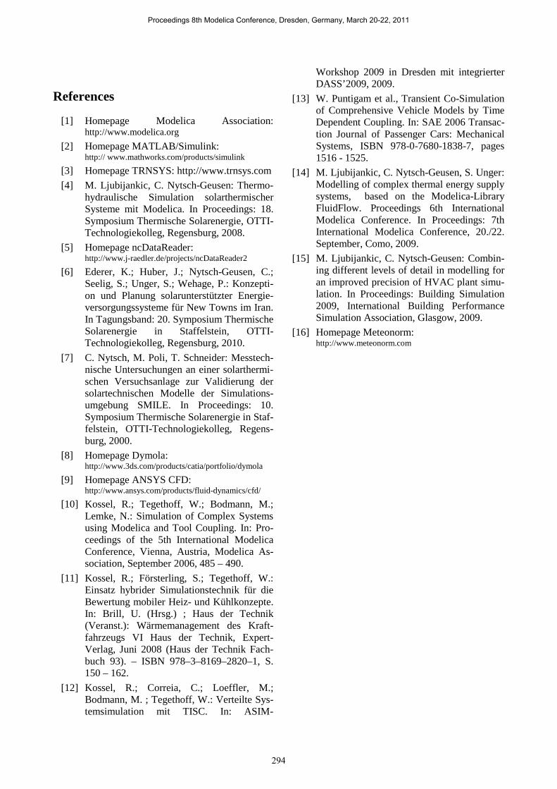
The TISC environment is divided in two layers, the Simulation-Layer and the Control-Layer. The Control-Layer is responsible for starting and parame-terizing all models at simulation start. It is also poss-ible to configure a set of simulations and let them run automatically one after another in batch-mode. This is helpful for using computer resources efficiently.

After a simulation has started, the Simulation-Layer is responsible for handling data-exchange and synchronization. Using the Control-Layer is optional and a distributed simulation can be performed using only the Simulation-Layer.

Figure 8: TISC synchronization scheme

TISC supports sequential (“explicit”) synchroni-

zation, while parallel (“implicit”) synchronization (see [13] and Figure 8) is often used. When using parallel synchronization all models are being calcu-lated simultaneously. With increasing number of models this leads to a major increase in simulation speed.

TISC uses fixed step-sizes for data-exchange be-tween the models and the server. The synchroniza-tion rate of the models has a highly influence on the total simulation time, because every time a model gets synchronized with the TISC server, depending on the used simulation program, an event is generat-ed and a convergent solution for the model has to be found again. With an increasing synchronization rate for system models with relative large time constants,

the number of synchronization events can be reduced and the simulation experiment can be relevant acce-lerated. It is also possible, that each model uses its own synchronization rate.

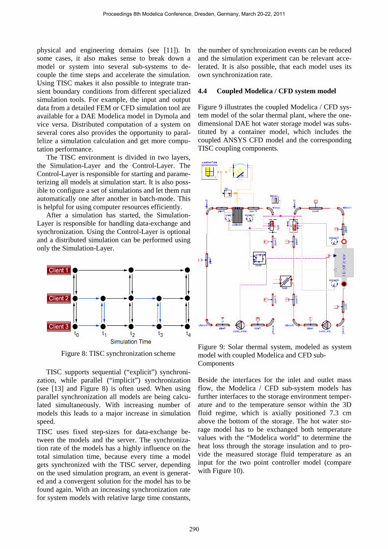
4.4 Coupled Modelica / CFD system model

Figure 9 illustrates the coupled Modelica / CFD sys-tem model of the solar thermal plant, where the one-dimensional DAE hot water storage model was subs-tituted by a container model, which includes the coupled ANSYS CFD model and the corresponding TISC coupling components.

Figure 9: Solar thermal system, modeled as system model with coupled Modelica and CFD sub- Components

Beside the interfaces for the inlet and outlet mass flow, the Modelica / CFD sub-system models has further interfaces to the storage environment temper-ature and to the temperature sensor within the 3D fluid regime, which is axially positioned 7.3 cm above the bottom of the storage. The hot water sto-rage model has to be exchanged both temperature values with the “Modelica world” to determine the heat loss through the storage insulation and to pro-vide the measured storage fluid temperature as an input for the two point controller model (compare with Figure 10).

Proceedings 8th Modelica Conference, Dresden, Germany, March 20-22, 2011

290

Figure 10: Modelica / CFD sub-system for the ther-mal storage

5 Comparative results of both simu-lation approaches

The Simulation experiment for the pure Modelica system model was performed with Dymola 7.4, us-ing the DASSL solver with a tolerance of 1e-4. The simulation model runs fast and needs only some seconds simulation time for one day real time.

In comparison to this, the coupled Modelica / CFD system model runs approximately half as fast as real time (≈ 50 hours simulation time). For this simu-lation experiment, an Apple MacPro workstation with 8 Xeon cores (2.8 GHz) and 32 GB RAM with the operation system Linux OpenSuse 11.2 was used. Doing this, ANSYS CFD used 8 cores for the paral-lelized CFD-simulation and Dymola used a separate core for the monolithic DAE-simulation on another Windows workstation. The synchronization rate of TISC was set on 1 second. Figures 11 to 14 illustrate the run of the curves for the most important state and process variables of the solar thermal system for a summer day in June (174th day of the year). Figure 11 shows the beam, diffuse and total solar irradiation on the tilted solar collector. The value for the total radiation exceeds 800 W/m2 at midday.

Figure 12 illustrates the inlet and outlet fluid temperatures of the solar collector and the outside air temperature for both simulation approaches. The ba-sic running of the temperatures values is similar (temperature levels, switching-on and –off events

etc.), but the values of the system with the CFD-storage model are more differentiated. The most im-portant reason for these differences consists in the non-existent momentum model within the DAE sto-rage model and its restricted space resolution to one dimension.

0

100

200

300

400

500

600

700

800

900

0 4 8 12 16 20 24

pow

er in

W/m

2

time in h

collector Gdot totalcollector Gdot direct

collector Gdot diffuse

Figure 11: Direct, diffuse, total solar irradiation on the tilted collector

10

15

20

25

30

35

40

45

50

55

0 4 8 12 16 20 24

tem

pera

ture

in C

time in h

collector T incollector T in (coupled)

collector T outcollector T out (coupled)

collector T env

Figure 12: Collector input and output temperature for the pure Modelica system model and for the coupled Modelica / CFD system model

0

0.005

0.01

0.015

0.02

0.025

0.03

0.035

0 4 8 12 16 20 24

mdo

t in

kg/s

time in h

pump mdot

0

0.005

0.01

0.015

0.02

0.025

0.03

0.035

0 4 8 12 16 20 24

mdo

t in

kg/s

time in h

pump mdot (coupled)

Figure 13: Mass flow of the collector and the storage pump for the pure Modelica system model (above) and the coupled Modelica/CFD system model (below)

Proceedings 8th Modelica Conference, Dresden, Germany, March 20-22, 2011

291

Figure 13 demonstrates the switching characteris-tic of the two-point controller at hand of the timeline of the mass flow, transported by the pumps. The ba-sic pattern of the mass flows for the pure Modelica model and the mixed Modelica / CFD model is simi-lar until 16 o’clock, when the solar irradiation inten-sity drops significantly. Then, differences in the con-troller behavior are clearly visible.

Figure 14 shows the inlet and outlet fluid temper-atures of the connection pipes between the storage sub-model and the rest of the solar thermal system model (indices plane in , plane out). Further, 10 rep-resentative temperatures within the storage fluid vo-lume are represented. For comparing the 10 vertical temperature values of the pure DAE Modelica model with the detailed temperature field of the CFD mod-el, integrated mean values over 10 horizontal vo-lumes were used (indices volume 1 to volume 10).

20

25

30

35

40

45

50

0 4 8 12 16 20 24

tem

pera

ture

in C

time in h

plane involume 1volume 2volume 3volume 4volume 5volume 6volume 7volume 8volume 9

volume 10plane out

20

25

30

35

40

45

50

0 4 8 12 16 20 24

tem

pera

ture

in C

time in h

plane involume 1volume 2volume 3volume 4volume 5volume 6volume 7volume 8volume 9

volume 10plane out

Figure 14: Inlet, outlet and layer temperatures of

the thermal storage for the CFD/FVM-model (above) and the Modelica/DAE-model (below)

The temperature levels in both storage models in-

crease during the day parallel to the stored thermal energy. The impact of the switch-on/switch-off cha-racteristic of the mass flows on the storage tempera-ture values developing can be clearly recognized during the morning hours and the evening hours. The CFD storage model shows a significantly more com-plex behavior: If the stored thermal energy flux

changes or the incoming mass flow switches be-tween zero and its maximum value, the CFD model shows an immediate reaction, because the momen-tum transport and the natural convection are part of the CFD algorithm.

Figure 15: Vertical section of the velocity field (left) and temperature field (right) after the first switch on event at 6:44 (above), at 13:00 (in the middle) and at 24:00, calculated by the coupled CFD/Modelica model

Proceedings 8th Modelica Conference, Dresden, Germany, March 20-22, 2011

292

An interesting phenomenon can be observed at the point plan in after sunset (→ mass flow of the storage pump equal to zero): During this time period, the DAE Modelica storage model shows an obvious temperature drop, while the temperature level on the same point of the CFD storage model has only a small decline. The reason for this difference lies in the natural convection effect, induced by the compa-ratively heat loss effect for the fluid in the small connection pipe in contrast to of the heat loss effect for the fluid within the storage. As a result, the natu-ral convection compensates the increased heat loss of the connection pipe by transporting additional ther-mal energy from the highest (and hottest) layer of the storage. This effect leads also to the greatest velocity in the region of the inlet connection pipe. The same phenomenon with the reinforced heat loss and the resulting induced convection can be recognized with-in the vertical sections of the temperature field and the velocity field at the end of the day (24 o’clock, compare with the third picture in Figure 15 and its enlargement in Figure 16).

Figure 16: Natural convection phenomenon (velocity field) at the inlet of the hot water storage CFD model at 24:00 Figure 17 illustrates the comparison of the calculated heat energies (supplied heat from the collector model and the inducted heat into the hot water storage) for the pure Modelica system model and for the coupled Modelica / CFD system model as integrated power values. During the whole load process there is only a very small difference between both simulation ap-proaches. The differences between the gained energy from the collector and the inducted energy into the storage are the thermal losses of the hydraulic com-ponents.

0

2

4

6

8

10

12

14

0 4 8 12 16 20 24

Q in

kW

h

time in h

supplied heat from collector (coupled)inducted heat into storage (coupled)

supplied heat from collector (not coupled)inducted heat into storage (not coupled)

Figure 17: Supplied heat from the collector model and inducted heat into the hot water storage for the pure Modelica system model and for the coupled Modelica / CFD system model

6 Summary and Outlook

It could be demonstrated by the example of a solar thermal plant, that the mixed DAE / CFD simulation approach works. This, the pure Modelica system model showed a qualitatively similar behavior (time-lines of the temperature and of the discrete controller events) and quantitative nearly identical energy val-ues in comparison to the mixed model. In addition, the detailed CFD sub-model of the hot water storage allows analysis for detailed questions (e.g. to find an optimized temperature sensor position or for study-ing convection phenomena) with full consideration of the surrounding system model. A sufficiently dis-cretized CFD model requires at a up-to-date comput-er hardware computing times twice as long as real-time. The next steps of the research will be a detailed analysis of the pressures losses within the different parts of the system (e.g. pressure fluctuations during discrete controller switching events). In addition fur-ther system models with more than one CFD sub-model (e.g. a collector CFD sub-model and a storage CFD sub-model) will be considered. For the accele-ration of the computation time of the coupled system model, the optimization of the numerical coupling parameters (e.g. the synchronization rate between both simulation tools) and parameter studies with different fine discretized meshes of the hot water storages will be considered.

Proceedings 8th Modelica Conference, Dresden, Germany, March 20-22, 2011

293

References

[1] Homepage Modelica Association: http://www.modelica.org

[2] Homepage MATLAB/Simulink: http:// www.mathworks.com/products/simulink

[3] Homepage TRNSYS: http://www.trnsys.com

[4] M. Ljubijankic, C. Nytsch-Geusen: Thermo-hydraulische Simulation solarthermischer Systeme mit Modelica. In Proceedings: 18. Symposium Thermische Solarenergie, OTTI-Technologiekolleg, Regensburg, 2008.

[5] Homepage ncDataReader: http://www.j-raedler.de/projects/ncDataReader2

[6] Ederer, K.; Huber, J.; Nytsch-Geusen, C.; Seelig, S.; Unger, S.; Wehage, P.: Konzepti-on und Planung solarunterstützter Energie-versorgungssysteme für New Towns im Iran. In Tagungsband: 20. Symposium Thermische Solarenergie in Staffelstein, OTTI-Technologiekolleg, Regensburg, 2010.

[7] C. Nytsch, M. Poli, T. Schneider: Messtech-nische Untersuchungen an einer solarthermi-schen Versuchsanlage zur Validierung der solartechnischen Modelle der Simulations-umgebung SMILE. In Proceedings: 10. Symposium Thermische Solarenergie in Staf-felstein, OTTI-Technologiekolleg, Regens-burg, 2000.

[8] Homepage Dymola: http://www.3ds.com/products/catia/portfolio/dymola

[9] Homepage ANSYS CFD: http://www.ansys.com/products/fluid-dynamics/cfd/

[10] Kossel, R.; Tegethoff, W.; Bodmann, M.; Lemke, N.: Simulation of Complex Systems using Modelica and Tool Coupling. In: Pro-ceedings of the 5th International Modelica Conference, Vienna, Austria, Modelica As-sociation, September 2006, 485 – 490.

[11] Kossel, R.; Försterling, S.; Tegethoff, W.: Einsatz hybrider Simulationstechnik für die Bewertung mobiler Heiz- und Kühlkonzepte. In: Brill, U. (Hrsg.) ; Haus der Technik (Veranst.): Wärmemanagement des Kraft-fahrzeugs VI Haus der Technik, Expert-Verlag, Juni 2008 (Haus der Technik Fach-buch 93). – ISBN 978–3–8169–2820–1, S. 150 – 162.

[12] Kossel, R.; Correia, C.; Loeffler, M.; Bodmann, M. ; Tegethoff, W.: Verteilte Sys-temsimulation mit TISC. In: ASIM-

Workshop 2009 in Dresden mit integrierter DASS’2009, 2009.

[13] W. Puntigam et al., Transient Co-Simulation of Comprehensive Vehicle Models by Time Dependent Coupling. In: SAE 2006 Transac-tion Journal of Passenger Cars: Mechanical Systems, ISBN 978-0-7680-1838-7, pages 1516 - 1525.

[14] M. Ljubijankic, C. Nytsch-Geusen, S. Unger: Modelling of complex thermal energy supply systems, based on the Modelica-Library FluidFlow. Proceedings 6th International Modelica Conference. In Proceedings: 7th International Modelica Conference, 20./22. September, Como, 2009.

[15] M. Ljubijankic, C. Nytsch-Geusen: Combin-ing different levels of detail in modelling for an improved precision of HVAC plant simu-lation. In Proceedings: Building Simulation 2009, International Building Performance Simulation Association, Glasgow, 2009.

[16] Homepage Meteonorm: http://www.meteonorm.com

Proceedings 8th Modelica Conference, Dresden, Germany, March 20-22, 2011

294