NUMERICAL AND EXPERIMENTAL ANALYSIS OF BREAKAGE IN A MILL

USING THE ATTAINABLE REGION APPROACH

by

MATTHEW JOSEPH METZGER

A dissertation submitted to the

Graduate School – New Brunswick

Rutgers, The State University of New Jersey

in partial fulfillment of the requirements

for the degree of

Doctor of Philosophy

Graduate Program in Chemical and Biochemical Engineering

written under the direction of

Professor Benjamin J. Glasser

And approved by

____________________________

____________________________

____________________________

____________________________

New Brunswick, New Jersey

October 2011

ii

ABSTRACT OF THE DISSERTATION

Numerical and Experimental Analysis of Breakage in a Mill Using the Attainable

Region Approach

By MATTHEW JOSEPH METZGER

Dissertation Director:

Professor Benjamin J. Glasser

Breakage of particulate materials is an essential process in many industries.

Despite its prevalence, size reduction is one of the most inefficient unit operations in the

collection of particulate processing operations. In this work, the breakage of granular

materials in a batch ball mill, a commonly encountered industrial system, was

investigated using computational and experimental techniques. Experimental analysis

was performed in a bench-top mill with size analysis through standard sieve screening.

Discrete element simulations (DEM) were carried out to examine the effect of a wide

range of particle and operational parameters. Both experimental and computational

results were analyzed using the Attainable Region (AR) approach.

Breakage was found to be dependent on grinding media fill level, mill rotation

rate, grinding media size and grinding time. At high energy inputs (large grinding media

fill levels and high mill rotation rates) breakage varied little. For lower values of these

parameters, breakage began to vary noticeably. The slowest mill rotation rate with the

largest grinding media size was optimal (in terms of both time and energy usage) to

produce the largest amount of a product of an intermediate size. It was also shown that

iii

variation of mill rotation rate could reduce the operating time of the mill by over 50%

with minimal sacrifice of desired product, and that the inclusion of a feed bypass in the

milling operation allows one to achieve product size distributions un-obtainable through

milling alone.

Computationally, single particle breakage simulations demonstrated agglomerate

breakage was not always directly proportional to impact velocity, and thus breakage was

a complex function of energy input. Good agreement between experimental and

computational trends in a batch ball mill was found and the majority of breakage in a ball

mill occurs near the mill shell, not at the surface where the grinding media and particles

make contact.

These findings contribute to the understanding of granular behavior in size

reduction environments. Improved understanding of the particle breakage phenomenon

will contribute to the development of more robust models and lead to improved energy

efficiency and reduced operational costs in the industrial processing of granular materials.

iv

Acknowledgements

I wish to thank many people who have offered invaluable guidance and assistance

along my path in graduate school. First, I would like to extend the most sincere gratitude

to my advisor, Prof. Benjamin J. Glasser, for his unwavering support and diligent

guidance throughout my tenure at Rutgers. He truly cared about my development and

ensured that my graduate experience was second to none. For that I am eternally

grateful. I thank my collaborators at the Centre of Materials and Process Synthesis

(COMPS) at the University of the Witwatersrand in Johannesburg, South Africa, Prof.

David Glasser and Prof. Diane Hildebrandt, for their unqualified encouragement. I thank

the other members of my committee, Prof. Henrik Pedersen and Prof. Nina Shapley, for

their feedback and comments. Thanks to Prof. Mike Moys, Prof. Rohit Ramachandran

and Prof. Troy Shinbrot for their insight and technical advice during the development of

my dissertation work. Many thanks to my undergraduate researchers Sachin Desai,

Anchal Jain, Hannes Pücher, Jason Selvaggio, Silvia Larisegger, Sarah Wilson, Kathryn

Camacho, Donald Legodi, Rhulani Makhubela and Nir Nativ for all their assistance.

To my fellow graduate students both at Rutgers, Brenda Remy, Xue Liu, Carolyn

Waite, Keirnan LaMarche, Eric Jayjock and Frank Romanski, and COMPS, David

Vetter, Ngangeze Khumalo and Tumisang Seodigeng; thanks for your encouragement

and the fun times. Finally, thanks to my family –Mom, Dad and Dan – and Becky for

their unconditional love and support that has made all of this possible. I would not be

where I am without you all by my side.

v

Table of Contents

ABSTRACT OF THE DISSERTATION ....................................................................... ii ACKNOWLEDGEMENTS ............................................................................................ iv

TABLE OF CONTENTS ................................................................................................. v LIST OF TABLES .......................................................................................................... vii LIST OF FIGURES ....................................................................................................... viii CHAPTER 1 BACKGROUND ................................................................................... 1

1.1 Motivation ...................................................................................................................... 1 1.2 Breakage Mechanisms ................................................................................................... 4 1.3 Theoretical Description .................................................................................................. 6 1.4 Breakage in a Ball Mill ................................................................................................ 11 1.5 Numerical Approach .................................................................................................... 18 1.6 Milling Optimization ................................................................................................... 29 1.7 Outstanding Issues and Path Forward .......................................................................... 33 1.8 Figures for Chapter 1 ................................................................................................... 35

CHAPTER 2 EXPERIMENTAL AND NUMERICAL METHODS ..................... 37 2.1 Experiments ................................................................................................................. 37

2.1.1 Material ........................................................................................................................ 39 2.1.2 Experimental Procedure ............................................................................................... 39

2.2 Numerical Simulations ................................................................................................. 40 2.2.1 Discrete Element Method (DEM) ................................................................................ 42 2.2.2 Bonded Particle Model (BPM) .................................................................................... 46 2.2.3 Geometry ..................................................................................................................... 48 2.2.4 Single Particle Breakage Metrics ................................................................................. 53 2.2.5 Ball Mill Simulation Metrics ....................................................................................... 53

2.3 Figures for Chapter 2 ................................................................................................... 56 CHAPTER 3 ATTAINABLE REGION ................................................................... 62

3.1 Background of the AR ................................................................................................. 62 3.2 Problem Statement ....................................................................................................... 64 3.3 Solution ........................................................................................................................ 65

3.3.1 Choose the Fundamental Processes ............................................................................. 65 3.3.2 Choose the State Variables .......................................................................................... 66 3.3.3 Define and Draw the Process Vectors .......................................................................... 67 3.3.4 Constructing the Region............................................................................................... 68 3.3.5 Interpret the Boundary as the Process Flow Sheet ....................................................... 69 3.3.6 Find the Optimum ........................................................................................................ 70

3.4 Conclusion ................................................................................................................... 71 3.5 Figures for Chapter 3 ................................................................................................... 72

CHAPTER 4 EXPERIMENTAL BREAKAGE WITH LARGE MEDIA ............ 78 4.1 Reproducibility ............................................................................................................ 78 4.2 Determination of Operational Capabilities .................................................................. 79 4.3 Minimization of Operating Time ................................................................................. 85 4.4 AR Extension Example ................................................................................................ 90 4.5 Recommendations for Continuous Operation .............................................................. 92 4.6 Conclusion ................................................................................................................... 93 4.7 Figures for Chapter 4 ................................................................................................... 95

CHAPTER 5 EXPERIMENTAL BREAKAGE WITH SMALL MEDIA .......... 106 5.1 Construction of the Attainable Region ....................................................................... 106 5.2 Effect of Grinding Media Size ................................................................................... 108 5.3 Effect of Grinding Media Fill Level .......................................................................... 109 5.4 Effect of Rotation Rate .............................................................................................. 110

vi

5.5 Optimal Production of Size Class Two ...................................................................... 111 5.6 Optimal Production of Size Class Three .................................................................... 116 5.7 Conclusion ................................................................................................................. 119 5.8 Figures for Chapter 5 ................................................................................................. 121

CHAPTER 6 NUMERICAL EXAMINATION OF SINGLE PARTICLE

BREAKAGE ...................................................................................... 128 6.1 Typical Behavior ........................................................................................................ 128 6.2 Effect of Bond Parameters ......................................................................................... 131 6.3 Effect of Test Parameters ........................................................................................... 139 6.4 Effect of Particle Parameters ...................................................................................... 144 6.5 Conclusion ................................................................................................................. 147 6.6 Figures for Chapter 6 ................................................................................................. 149

CHAPTER 7 NUMERICAL EXAMINATION OF BREAKAGE IN A BALL

MILL .................................................................................................. 159 7.1 Typical Behavior ........................................................................................................ 160 7.2 Effect of Critical Bond Strength ................................................................................ 162 7.3 Effect of Grinding Media Diameter ........................................................................... 167 7.4 Effect of Grinding Media Fill Level .......................................................................... 174 7.5 Effect of Drum Rotation Rate .................................................................................... 177 7.6 Optimal Production of Size Class Three .................................................................... 181 7.7 Conclusion ................................................................................................................. 184 7.8 Figures for Chapter 7 ................................................................................................. 187

CHAPTER 8 CONCLUSIONS AND FUTURE WORK ...................................... 196 8.1 Conclusions ................................................................................................................ 196 8.2 Future Work ............................................................................................................... 201

REFERENCES 205 CURRICULUM VITAE ............................................................................................... 213

vii

LIST OF TABLES

Table 2-1: Size classes. ................................................................................................................................. 56 Table 2-2: Base case Bonded Particle Model (BPM) input parameters for single particle breakage tests. ... 58 Table 2-3: Dimensions of the ball mill simulation. ....................................................................................... 59 Table 2-4: Input parameters for the base case ball mill simulation. .............................................................. 60 Table 2-5: Base case Bonded Particle Model (BPM) inputs for mill simulations. ........................................ 60 Table 2-6: Size classes used for agglomerate size distribution determination. ............................................. 61 Table 3-1: Reaction network constants and initial concentrations. ............................................................... 72 Table 4-1: Comparison of multiple speeds versus optimal speed policies. ................................................. 104

viii

LIST OF FIGURES

Figure 1-1: Major breakage mechanisms: (a) abrasion, (b) fracture and (c) cleavage, with (d)

corresponding particle size distributions [14]. ......................................................................... 35 Figure 1-2: Cross-sectional view of a ball mill with counterclockwise rotation. ........................................ 35 Figure 1-3: Rotating drum flow regimes as a function of increasing rotation rate: (a) Slipping (b)

Slumping (c) Rolling (d) Cascading (e) Cataracting (f) Centrifuging [54]. ............................. 36 Figure 2-1: Schematic of the batch ball mill setup. ..................................................................................... 56 Figure 2-2: Material in each size class. ....................................................................................................... 56 Figure 2-3: Schematic of (a) two particles in contact and (b) the contact model. ....................................... 57 Figure 2-4: Pictorial representation of the Bonded Particle Model (BPM) [150]. ...................................... 57 Figure 2-5: Single Particle Breakage (SPB) setup. ...................................................................................... 58 Figure 2-6: Agglomerate of 125 particles. ................................................................................................... 58 Figure 2-7: Ball mill simulation geometry. ................................................................................................. 59 Figure 2-8: Template used to create individual agglomerates. .................................................................... 60 Figure 3-1: Concentration as a function of space-time in a (a) PFR and (b) CSTR. Note that profiles for

CC and CD are not shown. ........................................................................................................ 73 Figure 3-2: State-space diagram. Point O represents the feed point. Point X represents an arbitrary CSTR

effluent point. The diagram on the top right is a PFR representing the PFR profile, J. The

diagram in the bottom left is a CSTR representing the CSTR locus ........................................ 74 Figure 3-3: Rate vectors of the fundamental processes involved in the example. The CSTR rate vector

points from the feed point, O, to the particular effluent point, T. The PFR rate vector is

tangent to the current concentration. The mixing rate vector is a stra .................................... 75 Figure 3-4: Determination of the Attainable Region. (a) Extension through mixing (dashed line); (b)

Extend with PFR in series [curve M]; (c) Resulting attainable Region (hatched) with

corresponding reactors. Note that (a)-(c) have an equivalent x-axis. (d) Reactor configuration

to achieve any point within the attainable region in (c). .......................................................... 75 Figure 3-5: Application of constraints on the attainable region. Point Y: maximum B produced in reaction

network. Point Z: maximum B produced given that CA must be greater than 0.6 kmol/m3. ... 77

Figure 4-1: Mass fraction of size class two vs. number of revolutions ( J = 1.5%). (a) c = 0.37; (b) c

= 0.21. Error bars represent standard deviations of 5 replicates. ............................................ 95

Figure 4-2: Class size distribution at c = 0.37 milling speed ( J = 1.5%). (a) Grinding profiles of all

six class sizes vs. time. (b) Grinding profiles vs. number of revolutions. (c) Cumulative mass

fraction vs. average particle size. ............................................................................................. 96

Figure 4-3: Construction of the attainable region (AR) for J = 1.5% and c = 0.37. (a) Mass fraction of

size classes one and two vs. number of revolutions. (b) Attainable region. ............................ 97 Figure 4-4: Variation of grinding profiles with speed for a high J . (a) Mass fraction of size class one vs.

number of revolutions. (b) Mass fraction of size class two vs. number of revolutions. (c)

Mass fraction of size class two vs. size class one. ................................................................... 98

Figure 4-5: Varying the number of grinding media at a single speed ( c = 0.21). J = 1.5% represents 1

grinding media, J = 10.7% represents 7 grinding media and J = 21.5% represents 14

grinding media. (a) Mass fraction of size class one vs. number of revolutions. (b) Mass

fraction of size class two vs. number of revolutions. (c) Mass fraction of size class two vs.

one............................................................................................................................................ 99 Figure 4-6: Varying speed with 1 grinding media. (a) Mass fraction of size class one vs. number of

revolutions. (b) Mass fraction of size class two vs. number of revolutions. (c) Mass fraction

of size class two vs. one. ........................................................................................................ 100 Figure 4-7: Varying speed with 1 grinding media. (a) Total energy drawn by mill (kJ) vs. number of

revolutions. (b) Mass fraction of size class two vs. number of revolutions. (c) Mass fraction

of size class two vs. total energy drawn (kJ). ......................................................................... 101

ix

Figure 4-8: Varying speed at low J to optimize a smaller size intermediate product. (a) Mass fraction of

size class two vs. number of revolutions. (b) Mass fraction of size class three vs. number of

revolutions. (c) Mass fraction of size class three vs. two. ..................................................... 102 Figure 4-9: (a) Single speed grinding profiles. (b) Optimal policies vs. single rotation rate runs. A

operates at c = 0.37 for 8 min followed by c = 0.03 for 75 min. B operates at c = 0.37

for 20 min followed by c = 0.03 for 37 min. ...................................................................... 103

Figure 4-10: Mass fractions of all six size classes of optimal Policies A and B when size class two reaches

its maximum point. ................................................................................................................ 104 Figure 4-11: Mass fractions of all six size classes of optimal Policies A and B when size class two reaches

its maximum point. (a) Attainable Region achieved will only milling. (b) Extension of the

Attainable Region possible through mixing. (c) Solution region satisfying the constraints of

0.2 < M1 < 0.4 and M3 > 0.25. ............................................................................................... 105 Figure 4-12: Schematic of ideal mill configuration for continuous processing of material. ....................... 105

Figure 5-1: Typical results from batch ball mill operation: J = 1.5% and c = 0.44. (a) Mass fraction of

each of the six size classes over time (b) Mass fraction of only the size classes of interest

versus number of revolutions ................................................................................................. 121

Figure 5-2: Construction of the Attainable Region for J = 1.5% and c = 0.44. (a) Mass fraction of M1

and M2 versus number of revolutions. (b) Attainable Region. ............................................... 121 Figure 5-3: Comparison between larger and smaller media at otherwise identical operating parameters. (a)

J = 10.7% and c ~ 0.25 (b) J = 1.5% and c ~ 0.25. .................................................... 122

Figure 5-4: Mass fraction of size class two vs. mass fraction of size class one for various levels of 25.4

mm grinding media at a single speed ( c = 0.17). J = 0.3% represents 1 grinding media, J

= 1.5% represents 5 grinding media, J = 4% represents 14 grinding media and J = 10.7%

represents 37 grinding media. ................................................................................................ 122 Figure 5-5: Mass fraction of size class two vs. mass fraction of size class one for various levels of 25.4

mm grinding media at a single speed ( c = 0.44). ................................................................ 123

Figure 5-6: Mass fraction of size class two vs. mass fraction of size class one for various rotation rates at a

grinding media fill level of J = 1.5%. .................................................................................. 123 Figure 5-7: Mass fraction of size class two vs. mass fraction of size class one for various rotation rates at a

grinding media fill level of J = 0.3%. .................................................................................. 124

Figure 5-8: Optimal production of M2 for each combination of J and c . Here, M2 is scaled to span the

range from 0 to 1. ................................................................................................................... 125 Figure 5-9: Overall optimal production of M2 from both media sizes, (a) versus M1 for low values of J

and (b) versus M1 for high values of J . ............................................................................... 126 Figure 5-10: Overall production of M2 versus energy utilization, (a) for low values of J and (b) for high

values of J . .......................................................................................................................... 126 Figure 5-11: Optimization of a particle size distribution. (a) M3 versus M1 at J = 0.3% (b) Preliminary

Attainable Region and the region satisfying the constraint (c) Extended Attainable Region

achieved through mixing (d) Solution to the presented constraints. ...................................... 127 Figure 6-1: Base case breakage over time: (a) 0.2 sec (b) 0.45 sec (c) 0.55 sec. Input parameters are

identical to those in Tables 2-2 and 2-4. ................................................................................ 149 Figure 6-2: High resolution imaging of an impact event. Particles are colored by their instantaneous

velocity, with the highest velocity red ( = 4.1 m/s) and lowest blue ( = 1.7 m/s). Identical

simulation conditions as Figure 6-1. ...................................................................................... 149

Figure 6-3: Breakage at 0.55 sec as a function of bond strength at a constant stiffness, nk = 1.0×109 Nm

-3.

max = (a) 5.0×108 Nm

-2 (b) 1.0×10

8 Nm

-2 (c) 5.0×10

7 Nm

-2 (d) 2.5×10

7 Nm

-2 (e) 1.0×10

7

Nm-2

(f) 1.0×106 Nm

-2. Instantaneous velocity of each particle is represented by its color

ranging from the lowest velocity of 0.56 m/s (blue) to the highest velocity of 3.8 m/s (red).150

x

Figure 6-4: Damage ratio (fraction of original bonds broken) as a function of bond strength for those cases

shown in Figure 6-3, at a constant stiffness of nk = 1.0×109 Nm

-3. ...................................... 151

Figure 6-5: Largest surviving progeny as a function of bond strength at a constant stiffness of nk =

1.0×109 Nm

-3. ......................................................................................................................... 152

Figure 6-6: Breakage at 0.55 sec as a function of bond stiffness at a constant strength, max = 1.0×10

7

Nm-2

. nk = (a) 1.0×109 Nm

-3 (b) 5.0×10

8 Nm

-3 (c) 1.0×10

8 Nm

-3 (d) 5.0×10

7 Nm

-3. Particles

are colored according to their instantaneous velocity with the highest velocity of 4.2 m/s

denoted by red and the lowest velocity of 1.7 m/s denoted by blue. ...................................... 153 Figure 6-7: Phase map of breakage types for various combinations of stiffness and strength. Blue region

(crosses) represents complete disintegration of the agglomerate. Green region (open squares)

represents no breakage of the agglomerate and yellow region (open circles) represents some,

but not complete, breakage of the agglomerate. Lower gray region represents the region of

unrealistic behavior. ............................................................................................................... 154 Figure 6-8: Damage ratios for agglomerates with two different resolutions. ............................................ 155

Figure 6-9: Largest surviving progeny as a function of impact velocity, at identical bond stiffness ( nk =

1.0×109 Nm

-3) and different critical bond strengths,

max = 1.0×107 Nm

-2 and

max =

2.5×107 Nm

-2. ......................................................................................................................... 156

Figure 6-10: Damage ratio (percentage of original bonds broken) as a function of impact velocity for

multiple bond strengths at a constant stiffness of nk = 1.0×109 Nm

-3. .................................. 157

Figure 6-11: Effect of coefficient of restitution (ep) on damage ratio at nk = 1.0×108 Nm

-3.

max =

5.0×106 Nm

-3. ......................................................................................................................... 158

Figure 7-1: Snapshots of flow at different times for the base case: c = 0.53, max = 1.0×10

8 Nm

-2, md

= 25.4 mm and J = 4%. t = (a) 0.7 s (b) 9.1 s (c) 9.2 s (d) 9.3 s (e) 9.4 s (f) 9.5 s. Flow

patterns repeat approximately every 0.5 seconds. Grinding media are colored grey. ........... 187

Figure 7-2: Construction of the Attainable Region for the base case simulation: c = 0.53, max =

1.0×108 Nm

-2, md = 25.4 mm and J = 4%. (a) Grinding profiles as a function of number of

revolutions (b) Attainable Region. ......................................................................................... 187

Figure 7-3: Snapshots of flow at 10 revolutions for various bond strengths (max ) at a rotation rate of c

= 0.53, J = 4%, md = 25.4 mm. max = (a) 1.0×10

8 Nm

-2 (b) 5.0×10

8 Nm

-2 (c) 1.0×10

9

Nm-2

. Each color represents 25% percent of the agglomerates originally created. ............... 188

Figure 7-4: Construction of the Attainable Region for variation in bond strength: c = 0.53, J = 4% and

md = 25.4 mm. (a) Grinding profiles as a function of number of revolutions (b) Attainable

Region. ................................................................................................................................... 188

Figure 7-5: Grinding media flow profiles for various bond strengths (max ) at a rotation rate of c =

0.53, J = 4%, md = 25.4 mm. max = (a) 1.0×10

8 Nm

-2 (b) 5.0×10

8 Nm

-2 (c) 1.0×10

9 Nm

-2.

Colors correspond to three different representative grinding media. ..................................... 188 Figure 7-6: Average number of contacts per time step between the grinding media and the mill shell, the

other grinding media and the individual particles as a function of critical bond strength. GM-

Part* and Part-Shell* are scaled by the number of agglomerates present in the system initially

(200) and Part-Part* is scaled by the total number of particles in the system (5400). ........... 189

Figure 7-7: Breakage event density map for various bond strengths (max ) at a rotation rate of c =

0.53, J = 4%, md = 25.4 mm. max = (a) 1.0×10

8 Nm

-2 (b) 5.0×10

8 Nm

-2 (c) 1.0×10

9 Nm

-2.

Color denotes frequency of breakage events and the scale is different for each figure. ........ 189

xi

Figure 7-8: Snapshots of flow at 10 revolutions for various grinding media sizes at a critical bond strength

of 1.0×108 Nm

-2, c ~ 0.53 and J = 4%. md = (a) 12.7 mm (b) 25.4 mm (c) 44.5 mm. Each

color represents 25% percent of the agglomerates originally created. ................................... 190 Figure 7-9: Grinding media profiles for various grinding media sizes at a critical bond strength of 1.0×10

8

Nm-2

, c ~ 0.53 and J = 4%. md = (a) 12.7 mm (b) 25.4 mm (c) 44.5 mm. Colors

correspond to three different representative grinding media. ................................................. 190

Figure 7-10: Velocity maps for various grinding media sizes at a critical bond strength of 1.0×108 Nm

-2, c

~ 0.53 and J = 4%. md = (a) 12.7 mm (b) 25.4 mm (c) 44.5 mm. Vectors represent average

grinding media velocity and color denotes fluctuation velocity of grinding media. .............. 190

Figure 7-11: Construction of the Attainable Region for variation in grinding media diameter: max =

1.0×108 Nm

-2, c = 0.53 and J = 4%. (a) Grinding profiles as a function of number of

revolutions (b) Attainable Region. ......................................................................................... 191 Figure 7-12: Average number of contacts per time step between the grinding media, the mill shell and the

individual particles as a function of critical bond strength. GM-Shell* and GM-GM* area

scaled by the number of grinding media in each case. GM-Part* and Part-Shell* are scaled by

the number of agglomerates present in the system initially (200) and Part-Part* is scaled by

the total number of particles in the system (5400). ................................................................ 191 Figure 7-13: Breakage event density map for various grinding media sizes at a critical bond strength of

1.0×108 Nm

-2, c ~ 0.53 and J = 4%. md = (a) 12.7 mm (b) 25.4 mm (c) 44.5 mm. Color

denotes frequency of breakage events.................................................................................... 192 Figure 7-14: Kinetic energy contours for various grinding media sizes at a critical bond strength of 1.0×10

8

Nm-2

, c ~ 0.53 and J = 4%. md = (a) 12.7 mm (b) 25.4 mm (c) 44.5 mm. Color denotes

kinetic energy of grinding media in mJ.................................................................................. 192

Figure 7-15: Construction of the Attainable Region for variation in grinding media fill level: max =

1.0×108 Nm

-2, c = 0.53 and md = 25.4 mm. (a) Grinding profiles as a function of number

of revolutions (b) Attainable Region. .................................................................................... 193

Figure 7-16: Snapshots of flow at 10 revolutions for various rotation rates (RPM) with max = 1.0×10

8

Nm-2

, md = 25.4 mm and J = 4%. c = (a) 0.10 (b) 0.30 (c) 0.53. Each color represents

25% percent of the agglomerates originally created. ............................................................. 193

Figure 7-17: Grinding media profiles for various rotation rates (RPM) with max = 1.0×10

8 Nm

-2, md =

25.4 mm and J = 4%. c = (a) 0.10 (b) 0.30 (c) 0.53. Colors correspond to three different

representative grinding media. ............................................................................................... 193 Figure 7-18: Average number of contacts per time step between the grinding media and the mill shell, the

other grinding media and the individual particles as a function of critical bond strength. GM-

Part* and Part-Shell* are scaled by the number of agglomerates present in the system initially

(200) and Part-Part* is scaled by the total number of particles in the system (5400). ........... 194

Figure 7-19: Construction of the Attainable Region for variation in drum rotation rate: max = 1.0×10

8

Nm-2

, J = 4% and md = 25.4 mm. (a) Grinding profiles as a function of number of

revolutions (b) Attainable Region. ......................................................................................... 194

Figure 7-20: Grinding media profiles up to 3 revolutions for various rotation rates (RPM) with max =

1.0×108 Nm

-2, md = 25.4 mm and J = 4%. c = (a) 0.10 (b) 0.30. Colors correspond to

three different representative grinding media. ....................................................................... 195 Figure 7-21: Optimization of a particle size distribution. (a) M3 versus M1 for various rotation rates. (b)

Preliminary Attainable Region and the region satisfying the constraint. (c) Extended

Attainable Region achieved through mixing. (d) Solution to the presented constraints. All

other parameters constant: c = 1.0×108 Nm

-2, md = 25.4 mm and J = 4%. ................... 195

1

Chapter 1 BACKGROUND

1.1 Motivation

Grinding and milling have been around for centuries. Mankind has always

needed to grind food and more recently mineral processing has necessitated the

introduction of milling as an industrial process [1]. In addition, size reduction processes

are common in industries ranging from paint to minerals extraction to pharmaceutical and

food production. In fact, the estimated energy consumption of all global comminution

operations is close to 6% of all electricity generated worldwide [2]. It would be expected

then that such common processes would be operating at near optimum efficiency, similar

to their counterpart fluid operations such as petroleum cracking and commodity chemical

production. However, this is not the case. For example, the energy efficiency of ball

milling, one of the simplest and most prevalent comminution operations, is around 25%

[3]. That means for every ten joules of energy provided to the mill, only 2.5 joules are

used to break the particles. The remaining 7.5 joules are lost as heat, noise or friction.

Based on the size of the industry, even a slight increase in the efficiency of comminution

processes can result in a significant reduction of energy requirements.

Possible reasons for this level of inefficiency are many, including technological

ones related to the lack of complete theories to describe the conversion of mechanical

energy into the creation of new surfaces, economical reasons related to the historically

inexpensive nature of energy and raw materials and conceptual reasons linked to the

perception that optimization of such a crude process is simple and not worth the effort.

In addition, the list of mill types is expansive, seemingly representing a different mill for

2

each application ranging from crushers to break meter long boulders to bench top agitated

media mills for nanogrinding. As a result, the applicability of those few comprehensive

investigations is often limited to that particular size reduction device. Still elusive is a

fundamental characterization of size reduction processes that can isolate breakage from

the numerous other events occurring simultaneously in a mill and suggest optimal

operating conditions to produce a desired product using minimal resources.

Traditional size reduction processes involve impacting a material with a ball,

wall, blade, hammer, etc, resulting in single or multiple breakage events, which produce a

size distribution with mean particle size less than the supplied particle size. Generally,

the most breakage arises from events of high energy intensity and events of lower energy

intensity produce the least amount of breakage. Required products from a milling

operation may vary slightly between industries, but all wish to reduce the size of the

supplied material only as far as necessary, for further reduction wastes time and energy.

Extensive breakage beyond the desired product size, or overgrinding, produces very

small particles, referred to as fines. The presence of fines can cause a variety of problems

for a particle handling process. First, fines can become entrained in the air, which

increase the possibility of dust explosions [4]. These plumes of particle laden air also

present exposure risks to personnel [5]. In addition, fines do not behave similarly to

larger particles of the same material composition [6]. Fines can develop stable arches at

the outlet of hoppers and stick to processing equipment, leading to reductions of overall

plant efficiency and increased downtime [7]. Also, the presence of fines in a milling

operation leads to a phenomenon known as the cushioning effect [8]. Here, the smaller

particles fill the voids between the larger particles, and when the larger particle

3

experiences a large force, this force is transmitted to the smaller particles, resulting in less

damage to the larger particle than if it were the only particle in the mill. Overgrinding is

a significant concern when milling shear and heat-sensitive materials, such as bio-

materials, food and pharmaceuticals [8]. As a result, rarely is the goal to reduce the

particle to the smallest size possible. Rather, the desired product is of an intermediate

size. Hence, milling operations are a balance between reducing the size of a particle and

minimizing overgrinding to maximize efficiency. Additionally, in the energy and

minerals extraction industries, energy usage is the dominant production cost, as the

material is inexpensive and throughput is on the order of tons. On the other hand, the

pharmaceutical industry processes a relatively small amount of material, but market

pressures necessitate a minimal time to market and a high level of process control.

Therefore, the optimization problem is multidimensional and changes depending on the

particular needs of the industry and product. What is lacking is an optimization approach

that is flexible enough to handle the various requirements of multiple industries, but

robust enough to effectively determine optimal operating parameters from bench scale to

production scale.

Milling is an extremely useful industrial process, especially in the pharmaceutical

industry, where its use is growing rapidly. Milling is often encountered after wet or dry

granulation in order to reduce the size of granules to increase flowability [9]. In addition,

milling is used to prepare uniformly sized seed crystals for crystallization processes and

to maintain desired product size after crystallization [1]. Perhaps the most prevalent use

of milling is to increase the surface area of drug crystals to increase dissolution [9, 10].

As newly discovered drugs continue to increase in complexity, so does their insolubility.

4

It is estimated that 40% or more of newly identified active substances are poorly water

soluble [11]. Milling, or grinding, has been identified as a means to facilitate formulation

and development and improve compound activity by maximizing the surface area

available for dissolution [12]. Dissolution time can be reduced at least 10 times, by

reducing the size of primary drug crystals from the micron to the sub-micron range [1].

However, milling drug crystals has led to polymorphism [13] and using different milling

technologies to perform the same size reduction has demonstrated varying dissolution

profiles [10]. Therefore, though extremely attractive as a means to address limitations of

newly discovered active compounds, much care is required to produce a final formulation

to achieve the intended therapeutic effect.

With this in mind, we explore the milling process with the goal of understanding

how reduction in particle size is affected by operational parameters through particle

dynamic simulations and experiments across the operation space. We then seek a

connection between the microscopic characterization of particles and the macroscopic

behavior in batch scale mills. This should answer questions such as “How will a particle

break given its material properties?” and “What are the ideal operational parameters to

produce a desired product size distribution?”

1.2 Breakage Mechanisms

Breakage can be divided into three major mechanisms, classified by how energy

is applied to a particle [14, 15]. Shown in Figure 1-1 are schematics and the resultant

particle size distributions from each breakage mechanism [14]. Abrasion or attrition,

shown in Figure 1-1(a), occurs when one large particle is reduced to one slightly smaller

particle and many tiny particles, producing a bimodal distribution. This is often the result

5

of glancing, low energy impacts. Breakage following this mechanism contributes

significantly to the production of fines that introduce process dangers and decrease

process efficiency. On the other hand, massive fracture shown in Figure 1-1(b), reduces

a single particle into many fragments of a variety of sizes, as a result of intense impacts

over a short time span. This distribution is extremely wide and is undesired when

attempting to control the output particle size from a mill. Finally, cleavage, as shown in

Figure 1-1(c), is often the result of slowly applied, high intensity stresses and produces a

few smaller particles of similar size. This distribution is the narrowest and is ideal when

attempting to tightly control the product particle size. Depending on the specific

operating and design parameters of the mill, any or all of the above mechanisms may

occur independently or simultaneously [14]. Each of these mechanisms corresponds to a

different energy input and resulting particle size distribution, hence it is difficult to

propose a single theory to capture the general behavior of breakage within a mill.

One of the major factors determining which type of breakage occurs during size

reduction is the strength of the particle being stressed. For a particle to be broken, the

forces which hold a particle together must be overcome. These forces are basically

chemical and therefore, comminution is essentially the conversion of applied mechanical

energy into chemical energy [16]. Fracture occurs at levels significantly below the

theoretical strength of a material because of the presence of preexisting flaws in the

particle microstructure, or cracks [17]. Chemical energy concentrates around these

cracks [5]. As the energy breaks the chemical bonds between atoms, the crack lengthens

creating two new free surfaces, increasing the surface energy and releasing the excess

energy as heat near the crack tip [3]. Fracture is produced when this crack extends to the

6

boundary of the particle at all points on the crack perimeter [16]. The weakest flaw

determines the particle strength, but it is not true that the weaker the particle flaw, the

easier it is to grind to a certain level [18]. Real particles fail asymmetrically due to

inhomogeneities in flaw strength and spatial distribution [19]. Therefore, identical

energy loads on two different particles can create vastly different breakage distributions.

In addition, cracks become less common as the particle size decreases, so there exists a

theoretical size below which it will not be possible to propagate a crack under any load

[5, 20, 21]. Nevertheless, replicating energy distributions between scales and machinery

has been the choice to date of researchers optimizing milling circuits.

1.3 Theoretical Description

To date the majority of breakage investigations view the process as a black box

operation, as milling is an intense and complicated process whose flow patterns and

dynamics are difficult to visualize. Few sensors can survive the destructive environment

[22, 23] and an understanding of milling is often hampered by the fact that descriptions of

granular flow are scarce and “not at all strong theoretically” [24]. Nevertheless, attempts

at a general theory have been made by many researchers. The three most commonly

referenced are those by Rittinger, Kick and Bond that attempt to relate the amount of

breakage to the energy input to the system [25, 26].

Rittinger’s theory [27] assumes the energy consumed is related to the new surface

area produced. His theory takes the form shown in equation 1-1,

12

11

DDKE (1-1)

7

where E is the energy consumed by the grinding process, K is a constant for a given

material and mill and 2D and 1D are the initial and final sizes, respectively, of the

particle. Fuerstenau and Abouzeid [3] compared quartz grinding results from many

researchers and found that the amount of new surface produced is directly proportional to

the energy expended, matching Rittinger’s theory. However, the surface energy of the

new surface produced is only on the order of 0.1% of the energy consumed by a typical

comminution operation [18]. Therefore, despite the agreement between the theory and

some well controlled experiments, the creation of new surface area alone cannot account

for all energy utilized during the breakage process.

Kick’s model [28] relates the energy consumed to the volume ratio between the

product and feed sizes. His theory takes the form of the equation,

2

1logD

DKE (1-2)

with the same definitions as above. Kick’s law assumes fracture is a result of

deformation right before fracture that is proportional to the feed particle size. This

deformation results in a strain energy on each particle, which leads to breakage [26].

Bond’s theory [29] assumes that every breakage event is part of a process

breaking a particle of infinite size into infinite particles of zero size, so the energy

required to break the larger particle into the smaller size is proportional to the difference

between the energies of the two particle sizes, as shown in equation 1-3 [25].

5.0

1

5.0

2

11

DDKE (1-3)

8

The 5.0

iD factor is derived from the crack length required to break a particle of size iD .

Since the surface area of unit volume of material is proportional to 1

iD , the crack length

in unit volume is considered to be proportional to one side of that area and, therefore,

proportional to 5.0

iD [25]. Bond’s equation has received the most attention as there is a

simple procedure [18] to determine the proportionality constant from laboratory

experiments: iWK 10 , where iW is the Bond Work Index. The Bond Work Index

essentially represents the resistance of a given material to crushing and grinding and

values for many common materials are readily available.

Despite the varying interpretations of the above models, some researchers suggest

that all three can be condensed into a single equation with a variable exponent relating

the energy consumed to the feed and product particle size, shown in equation 1-4 [26].

nx

dxCdE (1-4)

with n having the value: n = 1 (Kick), n = 1.5 (Bond) and n = 2 (Rittinger) [30].

Austin [26] states that these equations cannot be combined as such because the definition

of particle size varies between the three definitions, with Rittinger and Kick using a mean

particle size and Bond using “the size in microns which 80 percent passes”. As a result,

it is common to find both Rittinger’s law and Bond’s law match well with experimental

data over limited size ranges.

Each of these theories, though frequently cited and utilized, do not include

strength variations between particle sizes. As smaller particles are often much stronger

than their larger counterparts [20], this can result in major discrepancies between theory

and experiment. Morrell [31] has included an exponent in equation 1-4 that accounts for

9

size dependent strength variation, finding better match for data from industrial mills

producing particles in the range between 0.1 mm and 100 mm. However, including

breakage and its variation for different materials, as well as effects due to the presence of

a range of particle sizes, requires a considerably more complex model that limits the

applicability of these theoretical tools.

Another common approach to modeling size reduction is through the use of

population balance models (PBM) [32]. In population balance modeling, the size range

of interest is separated into discrete size intervals and the “birth” and “death” rates of

particles of all sizes are followed as a function of time [8, 30]. A larger particle is broken

(or dies) into many smaller particles that enter into a new, smaller size (being born), thus

completing the mass balance. There are four main categories of population balance

models: (i) discrete size, time continuous, (ii) discrete size, discrete time, (iii) size

continuous, time continuous and (iv) size continuous, discrete time [33]. Because

particle size is measured in size intervals, the first is the most common.

Particle birth and death rates are calculated using breakage kernels, which are

split into two empirically determined relations [8], called the selection function, which

represents the probability a given particle will be broken in the timeframe under

consideration, and the breakage function, which characterizes the distribution of the

resultant particles from that breakage event [34]. The selection function, iS , captures the

proportion of particles in size class i selected for breakage, and is a function of both the

mill operating parameters and the material [35]. The breakage function, ijB , is a lower

triangular matrix describing the amount of material broken from size class j into size

class i, and is assumed to be only a function of material parameters [36]. Values for these

10

parameters are normally determined empirically by matching breakage in a mill [37] or

from single particle breakage tests [38]. Taking this approach enables a complete

analytical solution to the amount in each size class as a function of time for a batch

milling process [30]. Varinot et al [14] used such an analysis to show that it was possible

to differentiate between various types of breakage in the wet phase grinding of carbon

particles in a stirred media mill. Herbst [39] showed the ability of the PBM approach to

capture breakage of limestone in a batch ball mill. These results were then used as a

basis for scale-up to commercial operation. Such a phenomenological approach provides

some idea of the macroscopic nature of the process, but as Kelly and Spottiswood [40]

describe, such parameters lump together all microscopic events and further investigation

is required to separate differing breakage mechanisms and understand fracture from first

principles.

Examination of milling distributions in this fashion has exposed the non-linear

behavior of breakage after an initially linear behavior; specifically, that the initial

grinding rates are not the same as extended grinding rates, do to temporally evolving

material properties and multi-particle interactions [41]. Austin [32] offers many

explanations for such non-linear breakage including measurement errors, changes in flow

profiles as a result of changes in charge particle size and a distribution of particle

strengths resulting in some particles that break easier than expected and some that remain

intact for longer. The most common explanation is the cushioning effect [8]. In addition

to reducing the efficiency of the grinding process, these phenomena also significantly

complicate the derivation of universal breakage kernels that compare well with

experimental results across multiple materials and pieces of equipment. Bilgili et al [42]

11

derived a time-variant PBM by including a temporal element in the breakage function to

match the non-linear breakage profiles of pigment particles. However, this complication

necessitates a numerical solution to the problem, removing some of the simplicity of the

approach. Furthermore, the additional parameters require validation, which requires

extensive experimentation and further restricts the results to specific machinery and

materials [41], and becomes almost prohibitive when working with fine particles [14].

Finally, the macroscopic approach of population balance modeling is a popular basis for

modeling of commercial grinding circuits [39], but it lacks the ability to isolate the

elementary processes involved in particulate size reduction, which can be essential to

determining resultant particle size distributions [43]. As a result, population balance

models are limited to an empirical description of the milling process, which leaves much

to be desired.

1.4 Breakage in a Ball Mill

One of the more simple units of size reduction is the ball mill. A cross-sectional

view of a counter-clockwise rotating drum is shown in Figure 1-2. Essentially it consists

of a cylinder, or mill shell, filled with the material to be reduced in size and grinding

media, meant to reduce the material to a smaller size. Rotation around the longitudinal

axis lifts the charge – grinding media and material – until the force of gravity exceeds the

centrifugal force and friction between the charge and the shell, and the charge separates

from the shell, forming the shoulder of the flow. The charge then enters flight or rolls

down the free surface to the lowest point in the shell, where it reenters the flow, also

known as the toe of the flow. Located in between the toe and the shoulder is the belly of

the load. Lifters are included along the periphery of the mill to aid the tumbling action.

12

The interior of the mill, both mill shell and lifters, is referred to as the mill liner. Contact

between the material and the much denser and massive grinding media leads to breakage.

Variations in the grinding media flow profiles produce a wide spectrum of collision

energies, which can influence the breakage behavior. There exist a myriad of options for

both grinding media and cylinder construction, but the most common system that will be

employed here is a steel drum and steel grinding media, i.e. steel spheres. Varying the

rotation rate and the size and number of grinding media makes it possible to evaluate a

wide range of energy inputs and track the resultant breakage on a few hundred grams, not

tons. The energy per unit time delivered to the mill to drive the rotation is referred to as

the power draw.

The key draw to ball milling is the ease and simplicity of operation. Little

attention is required from the operator and with enough time, a large range of fineness

final particle sizes can be achieved [25]. In addition, a ball mill can be operated

continuously, and even be partitioned to utilize grinding media of different size to

achieve a better final particle size distribution [44]. Recently, the stirred media variety

[45], which utilizes an impeller to agitate the charge and increase media-material

contacts, has received much attention due to the potential for extremely fine grinding in

the sub-micron range. Two even simpler varieties of ball mills are autogeneous (AG)

[25] and semi-autogeneous mills (SAG) [46], which use only large boulders of the same

material, or some larger boulders and a small amount of grinding media, respectively, to

perform the grinding. The advantage of these two types is lower chance of contamination

as a result of grinding and the reduced cost without the media. Also, from a research

perspective, the rotating drum (ball mill without breakage and media) is a regularly

13

encountered experimental apparatus used to capture unique granular patterns, including

axial band formation [47, 48], radial segregation [49], mixing dead zones [50] and sun

patterns [51]. Therefore, there is plenty of past research to refer to when examining the

flow of granular materials in a horizontally rotating cylinder.

Energy inefficiency is the main drawback of size reduction inside a ball mill. Ball

mills have demonstrated low levels of energy efficiency [3], which reflects the need to

assess and improve their performance. Lowrinson [25] finds that only 0.6% of the energy

input into a ball mill is actually used to create new surface area. Considering the size of

the comminution industry, that is an extreme amount of energy that is utilized for nothing

more than noise and heating rocks. Ball mills have also demonstrated numerous

problems industrially, including cyclic and surging behavior of the charge, erratic product

quality, high circulating ratio and unplanned shutdown [43]. Variation of grinding media

flow profiles produces a wide range of collision impact energies between all elements,

including media-media, media-mill and media-particle. Media-media and media-mill

contacts are inefficient because they have a low probability of contacting a particle, or if

they do, may not be intense enough to cause fracture [52]. Furthermore, inefficient

collisions and the ability of the particles to move freely inside the mill reduces efficiency

in two ways: first, conversion of media impact energy into particle translational energy

produces no breakage and second, the translation of the particles removes them from the

impact zone, decreasing the chance of media-particle contact [53]. Hence, though

frequently encountered, there are still many issues with ball mill operation that inspire

continued investigation.

14

The extent of grinding is determined by only a handful of design parameters. One

of the most influential is the rotational speed of the drum. A rotating ball mill

experiences flow regimes based on the rotation rate identical to those of a rotating drum,

as shown in Figure 1-3 [54]. At the lowest rotation rates, there is minimal friction

between the particles and the mill shell, and the particles slip, unaffected by the rotating

shell (Figure 1-3a). This is known as the slipping regime. Increasing the rotation rate

increases the interaction between the particles and the shell, as discrete sections of

material rise with the rotation to the highest point of the bed and then collapse in large

chunks down the free surface of the flow, forming the avalanching or slumping regime,

as shown in Figure 1-3(b). At higher rotation rates, the top surface is continuously

refreshing itself and forms a distinct angle with the horizontal known as the rolling

regime in Figure 1-3(c). Further increasing the rotation rate enters the cascading regime

of Figure 1-3(d), where the surface continues to refresh itself, though there is now an S-

shape to the surface, where the shoulder and the toe of the load are beginning to emerge.

At even higher rotation rates (Figure 1-3e), the particles at the uppermost part of the

surface (shoulder of the load) have enough energy to leave the bed and follow ballistic

trajectories towards the bottom of the surface (the toe of the load), called the cataracting

regime. At the highest rotation rates (Figure 1-3f), the centrifuging regime appears where

the particles are pinned against the walls of the drum and there is little relative motion.

The point at which this centrifuging occurs is referred to as the critical rotation rate, cN ,

calculated from equation 1-5 [55].

mm

cdD

N

2.42

(1-5)

15

Here mD is the mill diameter in meters and md is the diameter of the grinding media is

meters. Often, the mill rotation rate is expressed as a fraction or percentage of the critical

rotation rate.

Applied energy depends strongly on the motion of the media in the mill [56] and,

as demonstrated, the motion of the media depends strongly on the rotation rate. Hence,

the rotation rate will play a large role in determining the applied energy, which was found

to be constant for a given rotation rate [56]. Minimal particle movement in the extreme

rotation regimes (slipping and centrifuging) results in insignificant grinding action.

Bazin and Lavoie [36] found that grinding proceeds by attrition when operating in the

rolling and cascading regime, as the low energy intensity collisions chip off weaker edges

and corners of particles. Arentzen and Bhappu [57] suggest that the ideal regime for

grinding is the cataracting regime (see Figure 1-3e), where contacts between the aerial

grinding media and the material in the toe of the load are of the highest impact quality.

Impacts of this quality are desirable to produce breakage through cleavage; however, if

these contacts are too energetic, breakage will proceed through the massive fracture

mechanism that produces a wide range of product sizes. Therefore there exists a balance

between the media trajectory and the energy delivered by each collision. In addition, if

the rotation rate is not tuned properly, contacts between the media and the material may

not occur in the toe, resulting in inefficient collisions with the mill liner, or between the

media and material in the belly of the load. Collisions between media and liner lead to

significant liner wear, which shortens the lifetime and increases the material costs

associated with the mill [58]. On the other hand, collisions between the media and

material in the belly of the load are undesired because those collisions are highly

16

susceptible to the cushioning effect, which greatly reduces the grinding efficiency [43].

Evidently, the quality of media-material impacts can be tailored by manipulating grinding

media trajectories through rotation rate variation.

Another parameter that plays an important role in the grinding process is the

amount of grinding media. A convenient parameter often used to describe the amount of

grinding media in a mill is the fractional ball filling, J, which is the fraction of the mill

filled by the media bed at rest as defined by Austin et al [55]. Such terminology was

introduced because most industrial scale mills are meters in diameter and weighing the

grinding media is not feasible. But expressing the fraction of the mill volume occupied

by grinding media is a simple measurement that can be used to determine the mass or

number of grinding media in a mill. Shoji et al [59] found that there exists an optimal

ball fill for maximum breakage within the ball mill, where below this value too few

grinding balls limit the number of contacts between media and material, and above this

value contacts between media and material are limited by too many contacts between

media and other media. Similarly, Yokoyama et al [60] state that an excess of grinding

media decrease the energy intensity of collisions between the media and material, and

thus there is a balance between the energy of contacts and the frequency of those contacts

in order to produce the most of the desired material. Fahrenwald [61] reports that a mill

operating at 29% media fill level is more efficient than a mill operating at 45% media fill

because, among other benefits, there was less overgrinding with the smaller fill level.

Hence, less energy was lost to further breakage of the charge beyond the desired size.

A parameter that often leads to inefficient operation is the size of the grinding

media used [18, 57, 62]. Media must be larger than the feed material in order to achieve

17

breakage, but using media that are too large results in significant overgrinding as the

increased weight is much more than is required for a breakage event [63]. Therefore it is

desired to choose the size that will just break the largest particle in the feed [18]. A range

of formula exist to relate the size of grinding media ( md in mm) to the size of the feed

material ( mx in mm) and desired product size ( px in mm). Erdem and Ergun [62] cite

the classic equation 2

mm Kdx , where K is an empirically determined constant usually

between 10-2

and 10-3

[25]. Austin et al [63] extend the equation by varying the exponent

and the empirical constant to fit a variety of grinding experiments, finding that the

general theory of the form mm Kdx , holds reasonably well for between 0.5 and 1.

Alternatives to the above equation, i.e. 31

28 mm xd [44], mpm xxd log6 [44] and

md

m ex0346.0

2971.0 [62], also give good agreement with select sets of experimental data.

However, it is known that the feed size distribution, feed hardness, mill diameter, specific

gravity of the media and the mill rotation rate all affect the ball size selection, and none

of the above equations include any parameter except the average feed particle size. Bond

[18] presents a more comprehensive equation as shown,

31

21

100

m

mm

DCs

SgWi

K

xd (1-6)

where Sg is the specific gravity of the media, Wi is the Bond Work Index of the material

to be ground, Cs is the rotation rate of the mill and mD is the diameter of the mill. Yet,

there is still not consensus as to which equation yields the most reliable results. For

example, if the intention is to grind feed particles of average size 10 mm to an average

product particle size of 5 mm, the above equations suggest an optimal media size ranging

18

from 7 mm to over 100 mm. As a result, though extremely important to optimal grinding

efficiency, media size selection equations remain empirical and restricted to specific

applications. It is no wonder why grinding media size is not included in many of the

design and scale-up equations throughout the literature [25, 44, 55].

Yet another important parameter that determines the rate of breakage in a ball mill

is the fractional filling of material in the mill. Shoji et al [64] emphasize that there exists

an optimal fill level of material in order to achieve the highest rate of breakage. They

were able to develop a relationship between the fractional media fill and the fractional

material fill to determine the optimal fill levels for mills of differing diameter. They

suggest if the goal is to achieve a relatively large product size, to decrease the amount of

material in the mill.

1.5 Numerical Approach

Ball mills are simple in operation and analysis, but the ability to track and follow

the motion of individual particles and measure key process attributes, such as flow

profiles, mill power draw and impact energy spectra, is severely limited. However,

numerical investigations are not restricted by such limitations, and it is possible to

quantify and track many key process attributes. Discrete element method (DEM)

simulations, originally introduced by Cundall and Strack [65], have been used to simulate

various aspects of ball mill operation, from media flow profiles [43, 66], to wear on

lifters [58], to the effect of lifter height on power draw [67]. DEM simulations

completely characterize the microscopic contacts of many distinct granular objects,

which collectively establish macroscopic flow. Knowing the exact details of each and

every collision inside a mill is advantageous for many reasons. First, every collision

19

includes those of very low energy and high frequency, which are difficult to register with

conventional sensors [52, 68]. Each collision can be decomposed into forces created as a

result of friction, kinetic energy, breakage, etc [19], so it is possible to characterize the

division of energy in each collision, and thus isolate the main source of ball mill

inefficiency. Furthermore, analysis of the contact forces and progeny from each collision

helps to identify and encourage a particular breakage mechanism [69, 70]. An additional

functionality of DEM is the ability to alter material properties, i.e. Young’s modulus,

Poisson’s ratio, density, friction, etc, effortlessly to analyze efficiencies when processing

a wide range of materials [68, 71]. Also, DEM simulations remove some of the barriers

when attempting to derive a theory to describe flow and breakage in a ball mill. Whereas

theories to describe motion of granular materials in a complex geometry are limited [24],

it is straightforward to include the exact details of boundaries and foreign objects in DEM

simulations [72]. Through this approach it is simple to examine effects of altering

boundary conditions, such as liner and lifter profile and shape and their subsequent

effects on power draw and particle flow [73]. Finally, new geometry creation facilitates

comparisons between milling equipment without physically having the equipment [74].

DEM investigations of breakage have been performed in a variety of milling geometries

including shear cells [75], biaxial testers [76], stirred media mills [77], centrifugal mills

[78] and vibratory and planetary mills [72], just to name a few.

Combining the knowledge gained on the microscopic level can yield valuable

insight for operating more efficiently on an industrial scale. Following flow profiles can

help predict ideal operating conditions to ensure the most efficient collisions between

grinding media and material. Liner profiles can be designed and implemented to ensure

20

reproducibility of these ideal collisions and rotation rate effects can be incorporated to

introduce efficient control to a historically difficult to control process, due to feed

variations, complex interactions between numerous time-dependent and non-linear

process variables [79]. Ultimately, the goal would be to completely characterize

breakage on the microscopic, particle-particle level, which will then collectively correlate

to breakage on a macroscopic level, as part of a virtual comminution machine [69]. This

virtual tool could be used as a basis for confident and fundamentally sound design and

selection of efficient operating conditions of milling equipment [80].

The effectiveness of DEM modeling is not limitless. Computational constraints

have limited previous numerical investigations to small systems, or systems simulating a

characteristic particle size much larger than that in the actual mill [81]. Bilgili and

Scarlett [8] state that “DEM may not be predictive of milling at process length scale

because the number of particles that can be tracked is restricted to a few hundred

thousand to a million, whereas real processes can contain 109 - 10

12 particles.” Even

reducing system size may not be enough because the timescale of operation can be

enormous. It can take hours to simulate one second of real time operation, whereas an

industrial system can operate for hours, if not days [58]. As a result, researchers have

simplified the scenario somewhat by simulating large particles in small geometries and

extrapolating to the real mill size [23] or simulating truncated particle size distributions

[82].

In addition to system size limitations, model selection and validation is also of

concern for the credibility of DEM simulations. Standard linear [83, 84] and non-linear

[85] spring-dashpot DEM models have been used to simulate the operation of ball mills.

21

Although non-linear spring-dashpot models have been shown to be the most realistic

[86], computational constraints necessitate the use of linear models. Also, the linear

model has proven adequate for capturing general flow profiles and system dynamics [23].

Perhaps the most restricting aspect of model selection is determining realistic parameters

for the simulated materials [17, 87]. Many studies have focused on determining the

sensitivity of results to pertinent parameters, including material constants and simulation

conditions. Dong and Moys [88] found that the coefficient of restitution, which is the

ratio between the pre- and post-collisional velocities of an element, controls the stability

of grinding media flow, with intermediate values resulting in stable, reproducible flow,

and unsteady flow when the media have either high or low amounts of kinetic energy.

Investigations by Misra and Cheung [89] and Cleary [58] determined that the coefficient

of restitution had a minimal effect on the total power draw of ball mill. The impact of

friction coefficient between elements inside a ball mill is much more interesting. Van

Nierop et al [90] and Mishra and Rajamani [91] found that an increase in friction

coefficient resulted in an increase of up to 1.5 times in the mill power draw. However,

Misra and Cheung [89] found the opposite, that an increase in the friction coefficient

decreased the mill power draw. Cleary [58] and Djordjevic [67] observed a marginal

change in the mill power draw with varying friction coefficient. Analyzing the nature of

flow in the mill suggests that for cataracting flow, the friction coefficient should have a

minimal effect, as the collisions are more ballistic and the majority of energy is dissipated

through normal collisions. When the tumbling behavior is more similar to cascading

motion, frictional contacts dominate the flow, so a higher friction coefficient would

dissipate more energy, and require more power for operation. Therefore, selection of

22

material parameters must be performed with knowledge of the operational flow regimes

and their impact on macroscopic properties, such as power draw.

One approach to validation of material properties is to analyze the breakage of

single particles, either dropped from a certain height, or impacted by an object traveling

at a predefined speed, both experimentally and numerically. Simple in concept, single

particle breakage tests can offer much information about how a particle will break under

finely controlled conditions, which can then be correlated to breakage in an industrial

system. A variety of experimental systems are available [92-94], some with higher

scrutiny than others, but generally it is difficult to resolve the specifics of breakage

because of the size of a single particle, even smaller progeny and the miniscule timescale

of fracture [95]. DEM simulations do not suffer from such limitations, yet the

macroscopic results, i.e. resultant particle size distributions, can be matched to

experimental tests to determine the effects of test conditions and particle properties on

fracture. Essential to capturing realistic dynamics is high enough resolution between the

individual elements composing a single particle. Thornton and collaborators [95-97]

have simulated single particle breakage of spherical agglomerates held together through

surface adhesion forces between individual spheres. They found that the breakage is

dependent upon the arrangement of the particles, contact velocity, adhesion strength and

packing nature around the impact point [95]. Looser packed agglomerates would

disintegrate near the point of impact, but those fracture events would dissipate the

majority of the impact energy, leaving the remainder of the agglomerate relatively intact

[95]. Agglomerates impacting at high velocity also disintegrated, whereas there was

minimal breakage at lower impact speeds [96]. Agglomerate shape was also tested,

23

determining that cubical and cylindrical agglomerates dropped on their edges or corners

experienced less breakage than when dropped on a flat face, where they fractured into a

few (2-3) large fragments and many much smaller pieces [97]. Hence, breakage is

dependent upon many factors, including the test conditions, internal particle structure and

geometry of impact. Potapov et al [70, 71, 98] assembled agglomerates with bonds

connecting individual, unbreakable polygons. They discovered two types of breakage:

one at low to intermediate impact energies where large cracks produce large progeny,

resembling breakage by cleavage. Second, at higher energies the same primary cracks

possessed additional energy and branched to produce much smaller fragments. The

resultant breakage was similar to massive fracture, meaning that massive fracture could

be approximated by a series of cleavage events. Good agreement between experimental

single particle breakage data and simulation single particle breakage data was revealed,

strengthening the legitimacy of this approach as an effective means to determine particle

parameters [17, 84]. However, single particle breakage rarely occurs in a mill, so the

model must also be able to capture multi-particle interactions as well.

Preliminary DEM investigations have demonstrated its usefulness for analyzing

size reduction in a ball mill. Extensive comparisons have been performed matching

experimental grinding media flow profiles to simulated flow profiles, generally finding

good agreement between the two. Cleary and Hoyer [66] demonstrated very close

agreement between the flow of grinding media in a carefully monitored experimental

centrifugal ball mill and equivalent 2D DEM simulations. Van Nierop et al [90] found

similarly good agreement between their simulations and experiments, with a better match

demonstrated with the three versus the two dimensional simulation. Results from

24

Venugopal and Rajamani [23] support the excellent agreement between experiments and

three dimensional DEM and suggest that the simulations can be used to predict

component lifetimes by tracking the position and intensity of impacts of grinding media

with the mill shell and lifters over time. Cleary [58] does exactly this and finds that the

lifetime of ball mill liners can be increased by ~60% if rotation rate is decreased from

80% of critical speed to 60% of critical speed. Continuous adjustment of liner profile can

assist in evaluating their effect on charge motion and subsequently on mill efficiency to

pinpoint when it is necessary to replace the lifters. Simulations at various rotation rates

have identified the various flow regimes, opening the door for the potential to tune

rotation rate to promote more efficient collisions [99]. Furthermore, numerous

researchers have achieved excellent agreement with experimental power draw by

summing the total energy dissipated by all collisions inside the mill [23, 43, 66, 80].

Power draw has historically been one of the few readily available experimental

parameters, so not only is there an abundance of data for comparison, but a successful

comparison emboldens one to take full advantage of the plethora of information available

from DEM simulations.

One example of the power of DEM simulations is complete knowledge of the

forces associated with each impact. Not only can the simulations capture the impact

energy of each and every collision, even those below the limit of detection of most

experimental sensors, this information can be classified spatially and temporally to

determine regions of most efficient impact and how this distribution changes during mill

operation and as a function of operational parameters. Previous investigations have

found that the load experiences the highest strain at its deepest point closest to the toe

25

[46], networks of particles in contact (or force chains) exist throughout the mill and that

those particles with the heaviest load in the force chain contribute the most to

comminution inside the mill [99]. Knowing the strength of a representative particle

enables classification of each impact as causing or not causing breakage [89]. Such an

analysis is a numerical approach to determining values of the selection function. For

those impacts that are highly energetic but do not cause sufficient breakage, it is possible

to decompose the collision energy into contributions from breakage, translation, friction,

etc [53]. Results can be utilized to suggest adjustments to operating parameters to

promote more efficient collisions during ensuing experiments or analyses.

Another strength of DEM simulations is the knowledge of the position of each

particle throughout the mill. Granular materials are known for their ability to separate by

size, or segregate, during operation because large particles react differently than small

particles to the same applied force [100]. Such size segregation has been identified in

simple systems like a vertically vibrated cylinder [101, 102] or a simple shear device

[103], to more complex processes and larger scale events such as die filling of a tablet

press [104] and snow avalanches [105]. Understanding particulate segregation is the

driving force for the numerous studies on pattern formation in rotating drums mentioned

earlier and similar arguments can be used to explain segregation in a ball mill. Cleary

[58] and Agrawala et al [52] found that increasing the mill rotation from below the

critical rotation rate to near or above the critical rotation rate caused a well-mixed, or

random mixture, to segregate radially, with the larger grinding media towards the center.

Mishra and Rajamani [91] found the same behavior, but also saw the opposite at low

rotation rates, with the smaller particles forming the central, segregated core. When

26

operating in the cascading or rolling regime, a mechanism called percolation enables the

smaller particles rolling down the free surface to fit in the interstices between other

particles, which are unavailable to the larger media [106]. Thus, radial segregation is

observed, with the core composed of the smaller particles. At the highest rotation rates,

the opposite is observed for two reasons. First, the lighter material centrifuges first, so it

finds its way to the mill shell first, followed by the more massive grinding media [107].

In addition, percolation continues to enable the smaller particles to squeeze through the

voids in the granular bed and find their way to the walls [49]. Segregation is of interest

in ball mill investigations because a segregated flow will often have a poor grinding

efficiency. In either case mentioned above, the smaller particles targeted by the grinding

are shielded from high energy collisions by other grinding media [58]. Therefore,

collisional energy is dissipated through media-media contacts, rather than material-media

contacts. Such an analysis is yet another way to identify milling inefficiencies and then

suggest operating conditions to optimize grinding.

Simultaneous breakage and flow of discrete collections of particles in a mill has

not been previously investigated in much detail. Prior investigations have focused on a

single portion of the problem, such as the breakage of a single particle during impact [70,

71], fracture of solid blocks of rock given microscale input parameters [108, 109] or flow

of only monodisperse grinding media [67]. As breakage has been shown to be dependent

upon the instantaneous particle size distribution [8], it is crucial to examine milling

processes with simultaneous breakage and flow of all sizes to capture multi-particle

interactions such as the cushioning effect [59] and segregation [110]. Ideally, one would

like to be able to quantify macroscopic breakage and flow profiles from DEM

27

simulations using microscopic input parameters that are common and readily available,

e.g. Young’s modulus, Poisson’s ratio, etc. Once characterized, the effect of internal

flow and energy distribution on breakage profiles can be extended to large-scale mills,

which currently lack a formal design and optimization methodology [22].

A few investigators have taken variants of this approach to tackle the problem of

optimizing grinding in a ball mill. Bwayla et al [17] used a two part calculation to track

breakage in a SAG mill (a standard ball mill with only a small amount of grinding

media). First, 2D DEM simulations were used to produce impact energy distributions

over small time intervals. Combining the energy impact distributions with particle

surface area yields an empirical function describing how each energy event targets

particles of varying size. Inputting this function into an empirical breakage probability

function derived from single particle impact experiments determines whether a particle

breaks or not. Once broken, the particle is removed from the simulation. They find that

this approach over-predicts the breakage for many reasons, including the

oversimplification of the breakage based on the particle surface area and parameter

selection. Mishra [43] contends that given the impact energy spectra and the

corresponding breakage behavior of the particles, it is possible to make a direct

calculation of the resulting size distribution, and he shows good agreement with single

particle breakage data. Similarities exist between the breakage and selection function

used in this work and those associated with population balance modeling, however, both

still require empirical parameter determination and are computationally expensive.

Buchholtz et al [99] implemented 2D breakage of disks in a DEM routine using

selection and breakage functions. The selection function, or probability of breakage, was

28

based upon the stress needed to activate a flaw, i.e. convert a flaw into a crack, existing

within the vicinity of a contact between two particles. Progeny of the breakage event

were always circular, with one particle 75% of the size of the original particle and the

other particle’s size determined through mass balance. The main finding of the work was

that for autogeneous mills where there is no grinding media, the majority of the breakage

occurs deep within the bed, and does not occur as frequently on the surface where the

particles contact one another in a ballistic fashion. Force chains were cited as the main

reason for such breakage, as the force of impact was transferred through these chains to

the particles trapped near the mill walls, resulting in breakage. Such an analysis

demonstrates the ability of parameters and equations working at the microscopic level

producing macroscopic breakage and flow details. However, this analysis was limited to

two dimensions with only spherical particles and still required fine tuning of parameters

for the selection and breakage function.

Cleary [82] used a set of rules to determine when a spherical particle would break

and then replaced that parent particle with an appropriate distribution of spherical

daughter particles. A minimum fragment size specifies the smallest particle to be

resolved by the DEM routine. Breakage by impact and compression was enabled, so

breakage occurred when the flow circumstances dictated. Tests performed in a square

geometry captured the cushioning effect, where breakage diminished noticeably as the

presence of fines increased and insulated the unbroken larger particles from further

breakage. Full scale tests in a continuously operating ball mill suggest that the majority

of impacts in a SAG mill are not energetic enough to produce breakage upon first impact,

yet breakage still occurs [83]. Thus, cumulative damage plays an important role in SAG

29

grinding. A successful model of rock fracture must be able to resolve all types of

breakage events for particles of all sizes.

Herbst and coworkers [84, 111, 112] have incorporated the single particle

breakage approach of Potapov and Campbell [98] into a 3D mill simulation, known as

Discrete Grain Breakage (DGB). One of the goals was to learn more about the selection

function in order to refine its development for Population Balance Modeling (PBM).

Comparisons between cases after two full mill revolutions revealed a complex interplay

between power draw, breakage rate and flow profiles. In addition, such an approach

produced very good agreement with power draw as a function of rotation rate and product

size distribution from a SAG mill at scale with a truncated particle size distribution.

Material parameters were chosen from single particle breakage experiments and were

also incorporated into a SAG circuit performance simulator to predict equipment

performance [84]. Ultimately, the ideal combination will be determined by the needs of

the process, but the authors definitively demonstrate the utility of DEM to make this

determination.

Microscale DEM modeling has been shown to be extremely promising to model

ball mill circuits, but rigorous investigations are limited and still in their infancy. Much

work is required to continue to transition DEM modeling of milling from a

“guesstimation” tool to a legitimate option for designing and optimizing such systems.

1.6 Milling Optimization

Quantification of breakage and particle flow profiles would be the first step to an

effective optimization of milling processes from a theoretical prospective. Currently the

most common method employed to optimize comminution processes is to introduce a

30

classifier into the milling circuit to separate out the unmilled feed from the product

stream and return it to the mill. However, as milling equipment becomes more

specialized and smaller grinding products are desired, adequate classification equipment

may not exist [37]. Also, recycle is often frowned upon in the pharmaceutical industry as

it hinders the ability to monitor and track the lifecycle of ingredients throughout the

entirety of a pharmaceutical process train. Therefore, a method to optimize the resulting

particle size distribution from a mill without the use of a classifier or any additional

equipment is desirable.

Most recent work focusing on optimizing comminution processes is of a statistical

nature. Intelligently designed orthogonal experiments are used to elucidate the main

factors affecting the mean particle size and contributing to experimental variance. Some

examples of these statistical techniques are artificial neural networks (ANN) [113], the

Taguchi method combined with analysis of variance (ANOVA) [114], the response

surface method (RSM) [115] and the genetic algorithm (GA) [116]. Once the main

factors are known, optimal values for each input parameter can be chosen to optimize a

particular output parameter, i.e. specific surface area, average particle size or energy

consumption. The major drawback of these methods is the elaborate mathematics

involved with the experimental design and analysis.

Another approach to optimization that conforms with the desire to limit physical

changes to the comminution operation is systems optimization [117]. In systems

optimization, the goal is to optimize existing processes without replacing older, less

efficient equipment or incorporating new equipment. Thus, the overall capital utilization

of the equipment will increase, potentially greatly increasing the overall return from the

31

investment. Wibowo [118] stresses the potential of a systems perspective of granular

processes to approach the current operating efficiency of common fluid operations.

Related to systems optimization is the potential to optimize grinding processes

through physical arrangements of equipment. For most of the past century, cement

clinker, one of the most commonly ground materials, has been milled in a two

compartment tube mill: the first compartment containing larger grinding media to grind

the coarse clinker and the second containing smaller grinding media to perform the finer

grinding [119]. A similar arrangement has been suggested for optimal reactive grinding

in a vibration mill [120]. Studies in stirred media mills have recommended an alternative

configuration, where multiple passes through the same mill or associations of mills in

series may decrease the width of the resultant particle size distribution [37].

Deciding on the interconnectivity of multiple mills and their operating parameters

is not a trivial task. An optimization tool called the Attainable Region (AR) analysis first

introduced for optimizing chemical reaction networks with complex kinetics can be used

to construct the optimal configuration [121]. The methodology meshes extremely well

with the concept of systems optimization as the initial focus is on the fundamental

processes that occur in the system, rather than the pieces of equipment themselves. Then,

the optimization is performed and the optimal operating conditions and connectivity are

interpreted directly from the simple geometrical representations of the data, avoiding the

complex math involved with the previously mentioned statistical optimization techniques

and possibly leading to the discovery of new and improved milling configurations [122].

Similarities between comminution and chemical reaction suggest that the AR

analysis can be used to study comminution processes [123-125]. Khumalo et al [123]

32

developed a population balance model that described the comminution process in an

equipment independent fashion, relating the extent of breakage directly to the specific

energy input to the device. They theoretically demonstrated that the same net energy

input did not produce the same product particle size distribution and the AR could be

utilized to perform simultaneous process synthesis and optimization of the desired size

class. Optimal recommendations suggest that comminution equipment should be

assembled in series, rather than in parallel, and that a lower specific energy input is

required to produce the optimal amount of the desired intermediate sized product. The

authors validated their theoretical conclusions by showing good agreement between their

basic model and experimental results at different specific energy inputs [124]. In

addition, they extended their work from systems with only milling to those including

classification and recycle [125]. Katubilwa et al [126] utilized the AR analysis technique

in conjunction with a population balance model to track the breakage behavior of coal as

a function of grinding media diameter. They found that there was a relatively small

variation in breakage for larger grinding media sizes, whereas smaller grinding media

sizes increased the yield of fines (< 75 microns). This work will describe work done to

address a number of unanswered questions, as well as experimentally validate some of

the predictions of the AR analysis. In particular, Khumalo et al [123-125] focused on

achieving a desired product with optimal use of energy. In some industries (e.g. the

pharmaceutical industry) time of operation may be more important than energy usage,

thus it is imperative that an optimization strategy can adjust to the needs of various

industries.

33

1.7 Outstanding Issues and Path Forward

Predicting macroscopic operation based upon microscale material parameters is

still a daunting task for the comminution industry. Empirical relations and decades of

experience have served the industry well, however failure to incorporate breakage

kinetics and material transport dynamically can often lead to serious design errors. In

addition, little is known about the fundamental phenomena leading to breakage and how

such mechanisms translate into poor operational efficiency. What has yet to be seen is an

approach to handle the common variations in feed materials and stress application in a

simple mathematical framework.

A priori determination of optimal mill operating conditions is still nonexistent.

Studies have elucidated some of the basic occurrences on a single particle level, but

efficiency of commercial operations is dependent upon complex multi-particle

interactions and mill operating conditions. Phenomenological models cannot offer the

resolution required to identify breakage mechanisms and suggest conditions for more

efficient operation. Microscale modeling holds considerable promise, yet hurdles still

remain when marrying numerical approximations to the experimental system.

This work addresses a critical need to improve fundamental understanding of

breakage and suggest optimal milling conditions given a particle type. Chapter 2 outlines

the computational and experimental methodology and tools to be utilized to describe and

capture the milling behavior. The Attainable Region analysis used to characterize and

optimize the size reduction process is outlined in Chapter 3. Experimental results of the

impact of operating parameters on batch scale grinding are presented in Chapter 4 and

Chapter 5. Chapter 6 introduces a numerical approach to determine breakage

34

mechanisms and realistic material parameters. These parameters are implemented in

scale batch milling simulations in Chapter 7. Finally, conclusions are discussed in

Chapter 8, along with a discussion of future directions of research.

35

1.8 Figures for Chapter 1

Figure 1-1: Major breakage mechanisms: (a) abrasion, (b) fracture and (c) cleavage, with (d)

corresponding particle size distributions [14].

Figure 1-2: Cross-sectional view of a ball mill with counterclockwise rotation.

(a)

(b)

(c)

(d)

Lifters

Shell Media

Toe

Shoulder

Belly

Material

36

Figure 1-3: Rotating drum flow regimes as a function of increasing rotation rate: (a) Slipping (b)

Slumping (c) Rolling (d) Cascading (e) Cataracting (f) Centrifuging [54].

(a)

(d) (f)

(c) (b)

(e)

37

Chapter 2 EXPERIMENTAL AND NUMERICAL METHODS

Most industrial scale mills are operated without in depth knowledge of the

behavior within the mill. Increasing efficiency of operation can only start with a better

understanding of the microscopic behavior inside the mill. The ability to connect

characteristics of material flow to operating conditions is vital to comprehend the sources

of milling inefficiency. Studies on the bench scale make this information more

accessible, thus helping to increase the knowledge base to design more efficient

processes and perform adequate scale-up. Along this line, an experimental program has

been developed to investigate the breakage of particles in a batch ball mill in an attempt

to correlate microscopic breakage mechanisms to macroscopic operating conditions. In

addition, a numerical approach has also been established to fully classify breakage at

various conditions at the particle level and at a similar scale to the bench top experiments.

2.1 Experiments

Our milling apparatus is shown schematically in Figure 2-1. The batch milling

chamber (GlenMills, Clifton, NJ) is placed on a set of rollers (GlenMills, Clifton, NJ) that

rotates the milling chamber. The rollers can accommodate a single rotating drum.

Depending on the charge loaded in the mill and the rotational speed setting, the rotation

speed ranges between 3.5 RPM and 79 RPM. Two sizes of grinding media are used, both

chrome steel spheres, with the larger diameter equal to 44.5 mm and the smaller diameter

equal to 25.4 mm (GlenMills, Clifton, NJ). A common representation for the rotation

rate of a ball mill is as a fraction of the speed at which the material in the mill begins to

centrifuge [55], cN , where

38

mm

cdD

N

2.42

(1)

Here mD is the mill diameter in meters and md is the diameter of the grinding media in

meters. cN depends on the grinding media size, and is either 108 RPM for the large

media or 102 RPM for the small grinding media. Therefore, the resulting minimum and

maximum relative rotation rates of the drum are min,c = 0.03 and max,c = 0.72, with the

larger media and min,c = 0.04 and max,c = 0.77, with the smaller media, where c is the

rotation rate of the drum relative to cN . T1 is an optical tachometer (Monarch

Instrument, Amherst, NH) used to record the number of mill rotations. This signal is

relayed to the computer through the connector block (National Instruments, Austin, TX),

enabling continual data acquisition of the rotation rate. An On/Off Control has also been

incorporated, enabling computer control of the start and stop of the mill rotation.

Logging of the mill rotation rate and On/Off control is implemented through a computer

program written in LabVIEW. The power to the mill is monitored by a power meter

(Electronic Educational Devices, Denver, CO) that can record a variety of values,

including voltage, instantaneous wattage and overall power consumption.

Our rotating drum is a steel cylinder with a volume of 5 L with a length of 16.2

cm and diameter of 19.8 cm. The number of media initially loaded into the mill with the

material is represented by J , which is the fractional media filling, and is given by [55]:

6.0

0.1*

volumemill

density media / media of massJ (2-1)

This convention is used because industrial size ball mills can often be taller than most

people, so weighing the amount of media inside a mill is difficult, but determining the

39

media fill height is relatively simple [55]. To assist the tumbling of the media, two lifters

2.3 cm in height are spaced 180° from each other along the full length of the walls inside

the mill.

2.1.1 Material

The mill is initially charged with a predetermined amount of material to be milled.

Silica sand (FilPro 1/4"×1/8") purchased from Superior Pools (Piscataway, NJ) is used as

the test material in this investigation. The material is pre-screened and only the fraction

between 4 mm and 5.6 mm, (USA Standard Sieve Size No. 5 and 3 ½, respectively) is

kept for the initial charge to limit the variability of the feed material. For all results

presented in the following, an initial charge of 300 g of pre-screened material (size class

one) is loaded into the mill. All material is dry and stored in an environment where the

relative humidity ranges between 40% and 60%. As the material breaks, it is reduced in

size and enters into a different size class. For our investigation, we divide the size range

0 – 5.6 mm into six different size classes, with the topmost size fraction termed size class

one and the bottommost fraction termed size class six. Table 2-1 shows the distribution

of the size classes and Figure 2-2 shows photographs of each size class.

2.1.2 Experimental Procedure

The basic procedure is to grind a single charge for a certain amount of time, stop

the mill, screen the resulting mixture and weigh the material in each of the six size

classes. Material collected from the mill is loaded into the stack of sieves listed in Table

2-1 and shaken for 10 minutes on an Octagon 2000 sieve shaker. Particles are considered

to be in a certain size class if they are collected on the corresponding sieve listed in Table

40

2-1. Afterwards, the material is loaded back into the mill and the process is repeated.

The masses collected for each size class at each stoppage are plotted over time to develop

the grinding profiles for each size class, resulting in six separate curves for each run.

Each run at a specific setting of rotation rate, grinding media fill level and grinding media

size, is repeated a minimum of two times to ensure reproducibility. The effect of rotation

rate and grinding media fill level with large media is examined in Chapter 4. Chapter 5

reviews the effect of the same parameters with smaller grinding media, while also

comparing the results obtained between grinding media sizes.

2.2 Numerical Simulations

Experiments with granular materials are notoriously difficult for various reasons,

e.g. their opacity, humidity effects, particle-particle variations. Computational techniques

are not vulnerable to such factors, yet have yielded plentiful insight into numerous

systems of granular materials [127]. Unlike experiments with granular systems where the

opacity of the material restricts researchers to only surface measurements, a simulation

can follow each and every particle and easily determine flow patterns and particle

positions within the particle bed. Experiments can only illuminate part of the complex

picture of granular materials. In addition, changing a parameter in a simulation is

effortless, whereas for experimental systems, new materials/geometries need to be

acquired/constructed to investigate multiple properties. Hence, simulations can act as

inexpensive and quick design tools to determine the most important parameters in a test

system.

In general, there are three levels of granular modeling: macroscale, mesoscale and

microscale [128]. Macroscale, or continuum, models utilize volume or ensemble-

41

averaged quantities as inputs to particle species density, momentum and granular energy

balance equations to describe macroscopic properties such as velocity, concentration and

stress [129]. Basically, the approach extends the classical kinetic theory of gases to dense

particle flow, incorporating an energy dissipation term due to the inelastic nature of

collisions between granular particles [130]. Advantages of this approach include the

ability to model large systems with minimal computational expense, but each

complication of the system, e.g. size and density disparity, cohesion, etc, requires

extensive theoretical development [131]. Also, rarely do real granular flows exist near

the density of a dense gas, so questions remain about the applicability of such models to

slowly deforming flows with many contacts between elements [132]. Nevertheless, prior

investigations have demonstrated the ability to model Couette [133], channel [134] and

fluidized bed flow [130].

Mesoscale modeling divides a flow into regions, whose interactions are governed

by a set of rules, which match the phenomenology of granular flows. Cellular Automata

[135] and Monte Carlo [136] methods are two examples of mesoscale models that have

been used to study flow down chutes [137] and segregation in a rotating drum [138],

respectively. Such models are capable of capturing dynamics of large systems over long

times without the use of constitutive equations, but they lack the resolution to capture

individual collisions and model specific materials [139].

Microscale modeling characterizes a large number of particle level interactions to

establish bulk flow. One of the more widely used examples of microscale modeling of

granular materials, Discrete Element Method (DEM) modeling or Particle Dynamics

(PD) [65], has its roots in the modeling of molecules in statistical mechanics, referred to

42

as Molecular Dynamics (MD) [140]. The major difference between MD and DEM is the

inelastic nature of collisions between granular materials [141]. DEM models have been

used to simulate systems ranging from academic investigations of simple shear [142] to

large scale landslides [127]. Modeling every element and its interactions in a flow is

computationally expensive and tricks are often used to minimize computational burden,

including simplified boundary conditions [143] and dividing larger domains into periodic

slices for individual investigation [144].

2.2.1 Discrete Element Method (DEM)

Particle Dynamic simulations can be separated into two types, hard- and soft-

particle dynamics. In hard-particle, or event driven, dynamics, particles are assumed to

be rigid and collisions occur instantaneously, only with a single other element, i.e.

collisions are binary [141]. Knowing the position and velocity of each element enables

the creation of an events list enumerating all pending collisions. The simulation advances

to the next collision predicted by the list, evaluates the collision and rebuilds the collision

list. Energy dissipation is included with a coefficient of restitution, specifying the

reduction in post-collision velocity. As mentioned earlier, rarely do granular flows exist

in the low density regime where collisions are strictly binary and instantaneous.

Therefore, hard-particle dynamic simulations are limited as the solids fraction increases.

The model used in the work is a soft-sphere DEM model [145]. Unlike hard-

sphere dynamics, the time between iterations is held constant and sustained contacts of

finite time are allowed. Each particle is modeled as a deformable sphere with both

rotational and translational degrees of freedom. Forces on each particle (from

interactions with other particles, boundaries or external forces) are summed and

43

Newton’s equations of motion are integrated to determine the current and future positions

and velocities of each particle in the simulation space. The force on each particle can be

decomposed into a normal ( NF ) and tangential ( TF ) component and the motion of each

particle is described by the following

j

i

T

ij

N

iji

i gmFFdt

dvm (2-2)

j

rij

T

ijii

i FRdt

dI

(2-3)

where im , iR , iI , iv and i are the mass, radius, moment of inertia, linear velocity and

angular velocity of particle i and g is the acceleration due to gravity. rij is the

summation of torque caused by the contact force between particle i and j. Shown in

Figure 2-3(a) is a pictorial of the DEM model parameters.

2.2.1.1 Normal Impacts

The model used to describe the particle deformation during contact is that of

Tsuji et al [146] and is given by

4/12/3 ~~nnnnn

N kF . (2-4)

A pictorial of the force-displacement model parameters is shown in Figure 2-3(b). Here,

nk~

and n~ are the normal stiffness and damping coefficient, respectively. The first term

represents the non-linear repulsion experienced due to the overlap ( n ), whereas the

second term represents the non-linear dissipation during the contact, a characteristic

feature of granular materials. n is the normal overlap between particle i and particle j

calculated by

44

nRR jijin rr (2-5)

where the unit vector jijiijnn rrrr / points from the center of particle j to the

center of particle i. n is the rate of change of the normal overlap between the two

particles in contact. The normal stiffness is calculated from

2

*

13

2~

REkn (2-6)

with E the Young’s modulus and the Poisson’s ratio of the particle. *R is the

effective radius of the contacting particles and is given by

ji

ji

RR

RRR

* (2-7)

The normal damping coefficient is calculated from

22ln

~

ln3

52~

e

kme

n

n (2-8)

where e is the coefficient of restitution, which is kept constant.

2.2.1.2 Tangential Impacts

Analogous to the normal force, the tangential force is given by

4/1~~ttttt

T kF (2-9)

where tk~

is the tangential stiffness coefficient, t is the tangential displacement and t~

is the tangential damping coefficient. t is the rate of change of the tangential

displacement. The tangential stiffness is provided by Mindlin’s formula [147],

2/1

*

2

22~nt

GRk

, (2-10)

45

where G is the shear modulus of the particle. If the two particles are of different

materials with shear moduli 1G and 2G and Poisson’s ratios 1 and 2 , the parameters in

the above equations (2-6 and 2-10) are replaced with their effective values ( *E , *G and

* ) given by the following,

2

2

1

1

*

221

GGG

(2-11)

2

2

1

1

*

111

EEE

(2-12)

21

21*

. (2-13)

The tangential displacement is calculated by

dtv t

relt (2-14)

where t

relv is the relative tangential velocity of the colliding spheres and is defined by

jjiiji

t

rel RRsv vv . (2-15)

Here, s is the tangential component of the unit vector connecting the particle centers.

The Coulomb condition limits TF by NT FF to allow slip between the particle

surfaces and rolling friction is incorporated through RF N

rr . Throughout the

work, the tangential damping coefficient ( t~ ) is kept constant to the normal damping

coefficient ( n~ ). All simulations are carried out using the EDEM code by DEM

Solutions.

46

2.2.2 Bonded Particle Model (BPM)

A standard DEM approach does not allow for particle breakage. As such, primary

particles are bonded together according to the criteria specified by the Bonded Particle

Model (BPM). The BPM was first introduced by Potyondy and Cundall [109] as a

model to approximate the bonding within a large rock structure for strength and structure

analysis. Since then it has been used by other researchers [148-152], mostly to study the

strength of rock formations under stress. The challenge with modeling breakage is the

tendency of real materials to break into particles of unknown shape and dimension,

generally following predefined cracks already existing in the material. This is a problem

because the starting assumption with the most basic of DEM models is to approximate all

particles as perfect spheres. Any inclusion of shape variation increases the computational

demand greatly, and limits the size of the geometry and number of particles that can be

modeled. Therefore, the composite rock or particle will be assumed to be composed of

perfect spheres packed in some assembly with bonds between all particles meeting

certain restrictions, as demonstrated in Figure 2-4.

Each bond between two particles has strength in both the normal (tension) and

tangential direction, resisting the tendency of the particles to separate when a force is

applied. In addition to the characteristic parameters of the particles (R and nk~

), the bond

itself also possesses characteristic parameters. Think of the bond as a piece of cement

composed of a set of elastic springs distributed over a circular cross-section on the

surface of the particle that transfers both translational and rotational motion experienced

by one particle to the other particle it is bonded to. The incremental forces and moments

acting on the bond can be written as follows:

47

nnn UAkF (2-16)

sss UAkF (2-17)

nsn JkM (2-18)

sns IkM . (2-19)

Here A is the area of the cement bond (2RA ) and I ( 4

41 R ) and J ( 4

21 R ) are the

moment of inertia and polar moment of inertia of the bond, respectively. A contact

radius multiplier, , can be incorporated to vary the surface coverage by the bond.

Specifically,

ji RRR ,min . (2-20)

Each parameter is topped with a bar to differentiate it as a value of the bond,

rather than a value of the particle (a normal and tangential value for stiffness, radius and

forces in both the tangential and normal direction exist for both the bond and the particle

at this point). In addition, the is included because the force is incremental, which

carries forces and moments over between time steps. This means that the model can also

capture breakage as a result of contacts over a number of time steps. nM and sM are the

moments of the bond in the normal and tangential direction. nM captures the bending of

the bond, whereas sM captures the twisting of the bond or torsion. nF captures the

stretching of the bond in the normal direction and sF captures the stretching of the bond

in the tangential direction. Excessive forces or stretching by any of these four

mechanisms can lead to breakage. The equations used to determine when the force

exceeds a predefined level are derived from beam theory to be

48

c

sn

I

RM

A

F

max (2-21)

c

ns

J

RM

A

F max . (2-22)

Equations 2-21 – 2-22 are used to determine the normal and shear stresses on the bond (

c and c , respectively) and these values are compared to the critical normal and

tangential stress cutoff values, max and

max . If the cutoffs are exceeded, the bond

breaks. Otherwise, it remains intact. Both cutoffs do not need to be exceeded for the

bond to break, only one. A contact radius ( RC ) is specified to determine the maximum

distance two particles can be separated for them to be bonded.

Throughout the work presented here, the implementation of the BPM is limited to

monodisperse primary particles as well as uniform values of bond strength and stiffness

for each bond created.

2.2.3 Geometry

Two geometries are utilized in this work, a single particle breakage setup and a

batch ball mill. The single particle breakage setup approximates experimental drop-

weight tests, with a falling particle, rather than a dropping weight. In this test

experiment, a single particle is dropped from a pre-defined height, and the resultant

fragments produced are sieved to determine the breakage behavior of the material under

well-known loading conditions.

Figure 2-5 shows the geometry for the agglomerate impact tests. The constituent

particles are created, the bonds are introduced and then the agglomerate is dropped from

a height of 0.5 m towards an angled contact plate. A regular cubic lattice five particles in

49

each direction was used as the test agglomerate. An image of the agglomerate is shown

in Figure 2-6. 300 bonds are created, one at each of the contact points between the 125

particles of radius R = 0.0024 m in the agglomerate. A 5×5×5 agglomerate provides

enough particles to resolve some details about the impact events, with reasonable

computational expense. Input parameters for the bonds are given in Table 2-2. A note is

made there that the stiffness is represented with the units Nm-3

because it acts over the

cross sectional area specified by the bond-radius multiplier, . All of the results

presented in the following were performed at a constant stiffness

s

n

k

k and strength

ratio

c

c

, bond-radius multiplier ( ) and contact radius ( RC ). Brief investigations

into the effect of each of these parameters (not presented) revealed that the stiffness and

strength ratios have little effect on the results presented and as you increase the bond-

radius and the contact radius, the strength of the bonds increases. In addition, a

comparison is made between the extent of breakage of the 5x5x5 agglomerate and a

10x10x10 agglomerate. The 10x10x10 agglomerate is composed of 1000 primary

particles with half the diameter of those in the 5x5x5 agglomerate ( R = 0.0012 m),

resulting in identical overall agglomerate dimensions.

An angled plate is used because drop tests on a flat plate yielded unrealistic

separation of the agglomerate into layers as a result of the uniform strength of all bonds

throughout the agglomerate. The contact plate is rotated 45 degrees above the horizontal

(in the z-direction in our coordinates) and into the page (y-direction) to ensure the

agglomerate impacts only at a single point, and not along an edge before rebounding

away from the contact plate. After the agglomerate impacts the contact plate three main

50

types of breakage can occur: 1) complete disintegration, 2) no breakage and 3)

intermediate breakage. Complete disintegration occurs when all of the original bonds are

broken. No breakage results in an unchanged shape of the agglomerate and intermediate

breakage can yield a range of shapes and size distributions. Each of the particles (or

groups of particles) that is detached from the original agglomerate is referred to as a

daughter particle or progeny.

The origin of the system is centered below the contact plate. Particles are created

in a cubic lattice pattern in a box referred to as the agglomerate mold. Bonds between

neighboring particles are implemented, solidifying the spheres into a cube, or

agglomerate, with uniform void space between each particle. After bonding, gravity

carries the agglomerate from rest towards the contact plate. One of the aspects of this

work is to analyze the effect of impact velocity, which was varied by increasing or

decreasing the initial drop height of the agglomerate, to achieve a desired impact

velocity. If breakage occurs, the location, time and particles participating in the breakage

event are recorded for post analysis. The simulation proceeds until all particles have

come to rest. Effects of bonding parameters, impact velocity, agglomerate resolution and

simulation parameters on breakage are discussed in Chapter 6.

The second geometry is a horizontally rotating cylinder, fitted with two lifters

spaced 180 degrees apart, representing a batch ball mill. This geometry is shown in

Figure 2-7. Counterclockwise rotation proceeds around the central horizontal axis, with

the origin located in the center of the side of the cylinder nearest the reader. Dimensions

of the mill are listed in Table 2-1 and are chosen to match a 5 L batch ball mill. Baffles

are chosen to be 0.1617 m in length to span the entire length of the mill, 0.01 m in width

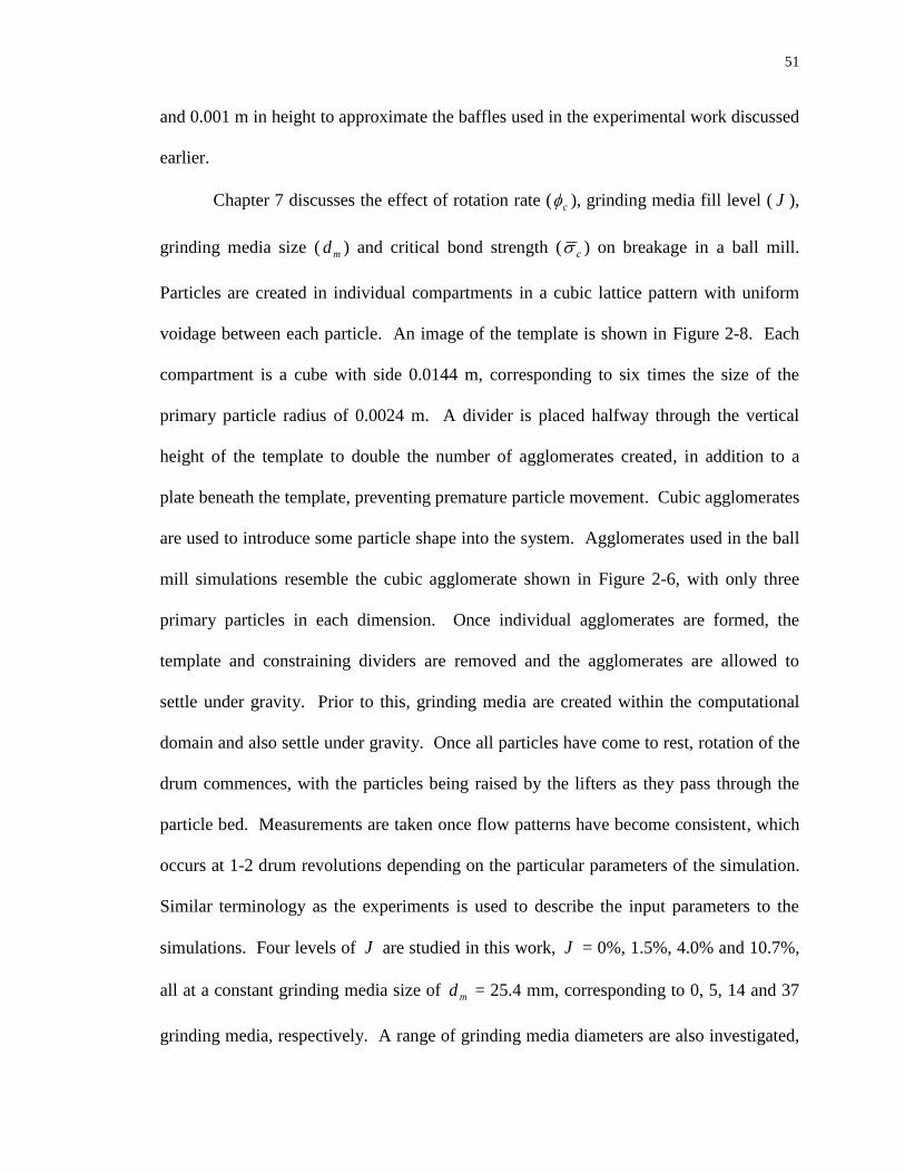
51

and 0.001 m in height to approximate the baffles used in the experimental work discussed

earlier.

Chapter 7 discusses the effect of rotation rate ( c ), grinding media fill level ( J ),

grinding media size ( md ) and critical bond strength ( c ) on breakage in a ball mill.

Particles are created in individual compartments in a cubic lattice pattern with uniform

voidage between each particle. An image of the template is shown in Figure 2-8. Each

compartment is a cube with side 0.0144 m, corresponding to six times the size of the

primary particle radius of 0.0024 m. A divider is placed halfway through the vertical

height of the template to double the number of agglomerates created, in addition to a

plate beneath the template, preventing premature particle movement. Cubic agglomerates

are used to introduce some particle shape into the system. Agglomerates used in the ball

mill simulations resemble the cubic agglomerate shown in Figure 2-6, with only three

primary particles in each dimension. Once individual agglomerates are formed, the

template and constraining dividers are removed and the agglomerates are allowed to

settle under gravity. Prior to this, grinding media are created within the computational

domain and also settle under gravity. Once all particles have come to rest, rotation of the

drum commences, with the particles being raised by the lifters as they pass through the

particle bed. Measurements are taken once flow patterns have become consistent, which

occurs at 1-2 drum revolutions depending on the particular parameters of the simulation.

Similar terminology as the experiments is used to describe the input parameters to the

simulations. Four levels of J are studied in this work, J = 0%, 1.5%, 4.0% and 10.7%,

all at a constant grinding media size of md = 25.4 mm, corresponding to 0, 5, 14 and 37

grinding media, respectively. A range of grinding media diameters are also investigated,

52

md = 12.7 mm, 25.4 mm and 44.5 mm, at a constant grinding media fill level of J =

4.0% (corresponding to 112, 14 and 3 grinding media of each size, respectively). Three

rotation rates are studied: 10 RPM, 30 RPM and 54 RPM. Again, the rotation rate is

expressed as a fraction of the speed at which the mill begins to centrifuge, which depends

on the grinding media size. is either 108 RPM, 101 RPM or 98 RPM for media of size

12.7 mm, 25.4 mm and 44.5 mm, respectively. Therefore, the resulting relative rotation

rates of the drum are c = 0.55 for 12.7 mm media, c = 0.53 for 25.4 mm media and c =

0.50 for 44.5 mm media, where c is the rotation rate of the drum relative to cN . When

comparisons are made between breakage at various rotation rates, the resulting relative

rotation rates of the drum are c = 0.10 for 10 RPM, c = 0.30 for 30 RPM and c = 0.53

for 54 RPM. Standard runs on a workstation with an Intel Core2 Duo 3 GHz processor

and 3 GB memory took about 1.5 hours of real time for every simulated second.

Base case input properties are listed in Table 2-4 for the standard DEM

parameters. The properties of the geometry elements and the grinding media are chosen

to match steel and the input parameters for the material are chosen to match those of

silica sand. A reduced value for the shear modulus was used to decrease computational

time, a reduction that has been shown in the literature to have negligible effect on flow

patterns and velocity profiles in non-bonded flows [145, 153, 154]. Inputs to the BPM

for the mill simulation are provided in Table 2-5. These parameters are chosen from the

analysis of the single particle breakage simulations, with the desire for most of the

agglomerates to survive the majority of the impacts experienced during ball mill

operation, but still be susceptible to breakage.

53

2.2.4 Single Particle Breakage Metrics

Quantifying breakage of agglomerates in the single particle breakage simulations

is done using a damage ratio metric, similar to that presented by Kafui and Thornton

[155]. A comparison is drawn between the bonds created initially and those remaining at

the conclusion of the breakage test using the equation

ndsInitial Bo

dsIntact BonDR . (2-23)

Here, BondsIntact is the number of bonds still in existence at the conclusion of the

single particle breakage test and BondsInitial is the total number of bonds created

initially. This metric is referred to as the Damage Ratio ( DR ) and will start at zero when

no bonds are broken and all are still intact, and increase to one as all bonds are broken as

a result of impact with the contact plate.

In addition to the Damage Ratio, agglomerate size distributions are prepared to

follow the breakdown of the initial agglomerate to individual progeny. Using the

breakage events output, the surviving agglomerate can be identified and a resultant

agglomerate size distribution in the range from single, primary particles to the initial

agglomerate size.

2.2.5 Ball Mill Simulation Metrics

Metrics used to analyze the batch ball mill focus on both breakage and flow of

agglomerates inside the mill. Key to both breakage behavior and charge motion is the

flow of grinding media in the mill, as that is the main avenue to deliver breakage energy

from the drum rotation to the agglomerates. To visualize the flow, steady-state positions

of representative grinding media (>2 revolutions) are plotted and connected. Following

54

the position of the grinding media provides evidence of the effect of the lifters on flow,

the flow regime of the mill charge and the disparities in flow from one media particle to

the next.

When a breakage event occurs, the position of that event is reported and can be

used to determine regions of breakage. Specifically, contour plots are prepared tracking

the frequency of breakage events throughout the mill domain, scaled by the total number

of breakage events for each set of simulations being compared. A high frequency of

breakage events corresponds to regions of significant breakage and low frequency values

represent regions of minimal breakage.

Another metric employed in the analysis of breakage in the ball mill is to track

and record the number and type of contacts between the grinding media, the particles and

the mill shell. Contacts between multiple grinding media and the grinding media and the

mill shell do not lead to breakage, and thus are undesired, inefficient collisions. Contacts

between the grinding media and the particles, the particles and the mill shell and between

multiple particles, on the other hand, may produce breakage and are thus efficient or

desired contacts. Classifying each contact in this manner provides some quantification of

the efficiency of energy transfer from the mill rotation to contacts potentially resulting in

particle breakage. Not every contact with an agglomerate results in breakage, but an

increased occurrence of contacts involving the agglomerates generally leads to an

increase in breakage observed.

Finally, similar information to the agglomerate size distribution utilized in the

single particle breakage simulations is collected to follow the extent of breakage as a

result of mill operation. As rotation proceeds, the agglomerates are reduced in size

55

starting from the initial agglomerate size of 27 and ending at the primary particle size of

one. The range is further divided into four sizes classes, which are displayed in Table

2-6. Lower-most bounds are selected to maintain an approximate size ratio of 2 , which

is a common ratio of size intervals for size reduction processes [156]. Agglomerate size

distributions are prepared by reconstructing the bond networks at each time step to

determine the size of the surviving agglomerates. From such information, grinding

profiles following the birth and death of agglomerates into intermediate product size

ranges and out of feed and intermediate size ranges as a function of number of drum

revolutions can be produced. In all of the cases presented here, rotation is stopped after

10 drum revolutions. This information is also used to construct the Attainable Region

(AR) curves which will be discussed in much more detail in the following chapters.

56

2.3 Figures for Chapter 2

Figure 2-1: Schematic of the batch ball mill setup.

Table 2-1: Size classes.

Figure 2-2: Material in each size class.

T1

Computer Mill

Connector

Block

On/Off

Control

Tachometer

Rollers

Speed Control

Power

Meter Power

Size Class Size Range (m) Sieve Number

One 5600 - 4000 5

Two 4000 - 2000 10

Three 2000 - 1000 18

Four 1000 - 600 30

Five 600 - 300 50

Six < 300 Pan

Size Class One Size Class Two Size Class Three

Size Class Four Size Class Five Size Class Six

5 mm 5 mm 5 mm

5 mm 5 mm 5 mm

57

Figure 2-3: Schematic of (a) two particles in contact and (b) the contact model.

Figure 2-4: Pictorial representation of the Bonded Particle Model (BPM) [150].

a

j

b

nk~

n~

tk~

im jm

j

jv

iv

NF

SF

i

58

Figure 2-5: Single Particle Breakage (SPB) setup.

Figure 2-6: Agglomerate of 125 particles.

Table 2-2: Base case Bonded Particle Model (BPM) input parameters for single particle breakage

tests.

z

x

y

Stiffness ratio

s

n

k

k 1.0

Normal stiffness ( nk ), Nm-3 1.0 × 108

Strength ratio

c

c

1.0

Tensile strength ( c ), Nm-2 5.0 × 106

Bond-radius multiplier ( ) 1.0

Contact radius ( RC ), m 0.2 × R

59

Figure 2-7: Ball mill simulation geometry.

Table 2-3: Dimensions of the ball mill simulation.

z

x

y

Mill Inner diameter (D), mm 198

Length, mm 162

Volume, L 5

Baffle height, mm 10

Baffle thickness, mm 1

60

Figure 2-8: Template used to create individual agglomerates.

Table 2-4: Input parameters for the base case ball mill simulation.

Table 2-5: Base case Bonded Particle Model (BPM) inputs for mill simulations.

z

x

y

Mill and grinding media Rolling friction coefficient, (r,m) 0.005

Sliding friction coefficient, (s,m) 0.75

Coefficient of resitution, (ep,m) 0.9

Density, (m) kg m-3

7800

Shear modulus, (Gm) Pa 5 × 107

Poisson's ratio, (m) 0.28

Grinding media diameter, (dm) m 0.01

Material Rolling friction coefficient, (r,s) 0.005

Sliding friction coefficient, (s,s) 0.75

Coefficient of resitution, (ep,s) 0.7

Density, (s) kg m-3

1220

Shear modulus, (Gs) Pa 5 × 106

Poisson's ratio, (s) 0.2

Particle diameter, (d) m 0.0024

Simulation parameters Timestep, sec < 1 × 10-5

Number of Particles, (N) 5,400

Stiffness ratio

s

n

k

k

1.0

Normal stiffness nk , Nm-3 1.0×109

Strength ratio

c

c

1.0

Tensile strength c , Nm-2 1.0×108

Bond-radius multiplier 1.0

Contact radius RC , m 0.2 × R

61

Table 2-6: Size classes used for agglomerate size distribution determination.

Size Class Agglomerate Size

One (M1) 26 - 27

Two (M2) 19 - 25

Three (M3) 13 - 18

Four (M4) 1 - 12

62

Chapter 3 ATTAINABLE REGION

A tool capable of optimizing a desired product from a milling operation must be

flexible, robust and simple. The ability to handle numerous constraints and objectives in

order to manage the variety of needs for various milling applications is essential. We

wish to develop a tool that is applicable across numerous industries and flexible enough

to deal with a wide range of optimization problems. In addition, the optimization tool

should be simple enough to make quick and meaningful decisions about the potential to

improve existing processes. In this chapter we overview the methodology of such an

approach referred to as the Attainable Region (AR) analysis. First, we present the origins

of the AR as a means to optimize networks of chemical reactions. Some alternatives to

solving chemical reaction engineering optimization problems are also reviewed. Then,

we introduce a commonly encountered problem in chemical reaction engineering and use

the Attainable Region analysis to solve the presented problem. Benefits of the Attainable

Region approach will be outlined from a problem-solving perspective as well as an

educational viewpoint. We then discuss how optimization of the comminution process

can be related to optimization of reaction networks. Such an analysis has application

beyond the fields of chemical reaction engineering and comminution, so it is hoped that a

general presentation of the approach will inspire utility in other fields in need of a

flexible, robust and simple optimization tool.

3.1 Background of the AR

The attainable region (AR) approach is a powerful research technique that has

been applied to optimization of reactor networks [157-159]. It is also a powerful

63

teaching tool that focuses on the fundamental processes involved in a system, rather than

the unit operations themselves. It has been used to introduce complex reactor network

optimization in a short time, with little to no additional calculations required.

The generic approach to complex reactor design and optimization is to build on

previous experience and knowledge to test a new reactor configuration against the

previous champion that yielded the best result [160]. If a new maximum is achieved, the

reactor configuration and process settings are kept, and if not, the previous solution is

retained and the entire process is repeated. The biggest issue with this trial and error

approach is the time it takes. Also, there is no way to know if all possible combinations

of operational parameters and reactors have been tested. In addition, calculations are

normally exhausting and general computational techniques are difficult to develop due to

the specificity of each arrangement. Over time, this mechanism has evolved into a set of

design heuristics that dominate decision processes throughout industry [161]. It should

be noted that optimization of the comminution process shares many features of this

heuristic approach.

Achenie and Biegler [162] model a reactor superstructure using a mixed integer

non-linear programming (MINLP), which transforms the task into an optimal control

problem. Again, this approach is useful if the optimal reactor network is known, but it

does not address the issue of choosing the optimal reactor network.

Horn [121] defines the Attainable Region (AR) as the region in the stoichiometric

subspace which could be reached by any possible reactor system. Furthermore, if any

point in this subspace were used as the feed to another system of reactors, the output from

this system would also exist within the same attainable region. This framework

64

approaches reactor design and optimization in a simpler, easier and more robust manner.

It offers a systematic, a priori, approach to determining the ideal reactor configuration

based upon identifying all possible output concentrations from all possible reactor

configurations. One of its advantages over previous approaches is the elimination of

laborious and counter-productive trial and error calculations. The focus is on

determining all possible outlet concentrations, regardless of the reactor configuration,

rather than examining a single concentration from a single reactor. Approaching the

problem from this direction ensures that all reactor systems are included in the analysis,

removing the reliance on the user’s imagination to create reactor structures. Also, for

lower dimensional problems, the final solution can be represented in a clear and intuitive

graphical form. From this graphical representation, the optimal process flow sheet can be

read directly. In addition, once the universal region of attainable concentrations is

known, applying new objective functions on the reactor system is effortless. No further

calculations are required, and the optimal values can be read directly from the graph.

Finally, this general tool can be applied to any problem whose basic operation can be

broken down into fundamental processes, including isothermal and nonisothermal reactor

network synthesis [157, 163], optimal control [164], combined reaction and separation

[165-167], comminution [123] and others. Process synthesis and design usefulness is

aided greatly by this alternative approach.

3.2 Problem Statement

The following liquid phase, constant density, isothermal reaction network will be

used to illustrate the attainable region approach.

65

CBAkk

k

31

2

(3-1)

DAk4

2 (3-2)

The initial characteristics of the reaction network are shown in Table 3-1. The end goal

of this exercise is to determine the reactor configuration that maximizes the production of

B for a feed of pure A. These reaction kinetics were used as they represent a reaction

network without an intuitively obvious optimal structure. A PFR will maximize the

amount of B produced in the first reaction, but a continuously stirred tank reactor (CSTR)

will minimize the amount of A consumed in the second reaction.

3.3 Solution

Determining the candidate attainable region for this reaction scheme involves the

completion of the following simplified steps: selecting the fundamental processes,

choosing the state variables, defining and drawing the process vectors, constructing the

region, interpreting the boundary as the process flow sheet and finding the optimum.

3.3.1 Choose the Fundamental Processes

In this particular example the fundamental processes are reaction and mixing. Let

us first look at mixing. There are two limits on mixing in a reactor: a plug flow reactor,

in which a slug of fluid does not experience any axial mixing along the reactor length and

a continuously stirred tank reactor, in which each volume element experiences complete

mixing. Before moving further into the analysis, it is useful to determine the dependence

of species concentrations on space-time in these two environments. For a PFR, this is

66

determined by numerically solving the mass balances in equations (3-3)-(3-6), giving the

concentration profiles of CA and CB in Figure 3-1(a).

2

421 ABAA CkCkCk

d

dC

(3-3)

BBAB CkCkCk

d

dC321

(3-4)

BC Ck

d

dC3

(3-5)

2

4 AD Ck

d

dC

(3-6)

Similarly, the set of mass balances in (3-7)-(3-10) can be solved to give the locus for a

CSTR as τ is varied, provided in Figure 3-1(b).

2

421

0

ABAAA CkCkCkCC (3-7)

BBABB CkCkCkCC 321

0 (3-8)

BCC CkCC 3

0 (3-9)

2

4

0

ADD CkCC (3-10)

In equations (3-3)-(3-10), Ci represents the concentration of species i, Ci0 represents the

feed concentration of species i, τ is the space-time of the reactor, and kj represents the rate

of reaction j. Figure 3-1 only shows the profiles for CA and CB because, as will be

explained shortly, CC and CD do not influence the determination of the AR.

3.3.2 Choose the State Variables

The state variables for this example are CA and CB. CB is a state variable because

it is the value which we wish to optimize. CA is a state variable because, looking at the

right hand side of equations (3-3) through (3-10), the behavior of CB is entirely dependent

67

on the change in CA. Note that τ is not a state variable because it is the independent

variable in the system. Because we only require two state variables, the solution can

easily be presented in a two dimensional plot.

Now that the state variables are known, a state-space or phase-space diagram

[168] (Figure 3-2) can be created showing the autonomous relation between CA and CB.

First, we do this for the PFR using the data in Figure 3-1(a). Figure 3-1(a) shows CA and

CB as a function of , so for any given we can determine a CA, CB pair which allows us

to map the concentrations in state-space and plot curve J (solid line) in Figure 3-2. For

example, the point W in Figure 3-2 corresponds to CA = 3.81×10-2

kmol/m3 and CB =

3.95×10-5

kmol/m3 and can be traced back to = 0.25 sec in Figure 3-1(a). The same can

be done for the data in Figure 3-1(b) for the CSTR which leads to curve K (dashed line)

in Figure 3-2. Under each curve is a typical representation of that particular reactor type.

Here, point X is an arbitrary CSTR effluent point used in the analysis later. While space

time is not explicitly shown in Figure 3-2, the relevant space time to achieve a given

concentration can always be obtained from Figure 3-1 (or an equivalent figure). A

candidate for the attainable region (ARC) is identified as the union of the regions

contained under both curves.

3.3.3 Define and Draw the Process Vectors

A process vector gives the instantaneous change in system state caused by that

fundamental process occurring. For example, if only reaction is occurring the reaction

vector, r[CA, CB], will give the instantaneous direction and magnitude of change from the

current concentration position. For mixing, this vector gives the divergence from the

current state, c, based upon the added state, c*, or v(c, c

*) = c

* - c.

68

The vectors can be graphically represented by considering curve K for the CSTR

in Figure 3-2. Curve K is replotted in Figure 3-3 along with the directions of the rate

vectors associated with the two limiting reactor cases (CSTR and PFR). Both X and T

are some arbitrary effluent concentrations from a CSTR shown strictly for demonstration

purposes. The CSTR rate vector (OT) is co-linear with the feed and effluent

concentrations, and the mixing vector (OX) linearly connects the two points representing

the solutions to be mixed. The resulting mixed state lies on the mixing line and its

position can be determined from the Lever Arm Rule [169]. One can also consider a PFR

rate vector which originates at the current concentration and is tangent to the curve (see

Figure 3-3).

3.3.4 Constructing the Region

To construct the region, the process vector guidelines from the previous step are

applied to the state-space diagram (Figure 3-2). The idea is to draw process vectors to

extend the current candidate attainable region (ARC). We begin the analysis by

examining mixing.

Starting at a generic point X on the boundary of curve K in Figure 3-2, a straight

line can be drawn to point O, which is the feed point. This is shown by line L in Figure

3-4(a). To achieve any concentration along line L you can mix the outlet of a CSTR

operating at point X with the feed at point O. Thus any point on curve L corresponds to a

CSTR with bypass. The Lever Arm Rule [169] can be used to determine the percentage

of each stream to mix to obtain the desired concentration. Notice that when this line is

drawn, the candidate region is extended. When two states mix linearly, mixing can

extend any concave region by creating its convex hull.

69

Does operation in a PFR extend the region as well? The answer is yes. Going

back to the process vector geometry, the PFR process vector is tangent to the current

system state. A line tangent to the curve at point X extends the region above its previous

maximum. The complete successive PFR profile (curve (M) in Figure 3-4b) is found by

numerically solving the differential PFR balance equations in (3-3)-(3-6) with feed

concentration of X = (CA, CB). The boundary of the current candidate attainable region is

now made up of curves (L) and (M) (see Figure 3-4b).

The attainable region can be constructed once it has been determined that no other

processes can extend the region. The shaded region of Figure 3-4(c) shows the entire

attainable region for this particular reaction network. The boundary of the shaded region

is made up of curves (L) and (M). Since the region is convex, it is clear that mixing

cannot extend the region. Moreover, it is possible to show that all rate vectors on the

boundary are either (i) tangent to the boundary or (ii) point into the region. Enclosed

beneath the boundary are all possible reactor effluents given a feed at point O.

3.3.5 Interpret the Boundary as the Process Flow Sheet

The process flow sheet is determined by tracing a path to the point of interest.

The effluent concentration at point X is achieved in a CSTR. If the desired effluent is to

the right of point X on the boundary (lying on curve L), a CSTR operating at point X

with feed bypass is used to reach the point. If the desired effluent is on the boundary to

the left of point X (lying on curve M), a CSTR operating at point X followed by a PFR in

series is required. These configurations are pointed out in Figure 3-4(c). The reactor

configuration in Figure 3-4(d) can be used to achieve any point on the boundary of the

ARC for this reaction network.

70

3.3.6 Find the Optimum

The final step is to determine the optimum for the specified objective function. In

this case, the objective function is to maximize the production of species B given the feed

of 1 kmol/m3 of A. It can easily be seen from Figure 3-5 (point Y) that a maximum of

1.24×10-4

kmol/m3 species B can be achieved using a CSTR with effluent of 0.4 kmol/m

3

species A followed by a PFR with an effluent concentration of A of 0.18 kmol/m3. The

corresponding space-times of the CSTR and the PFR are 0.037 sec and 0.031 sec,

respectively. These were determined from equations 3-7 and 3-8 for the CSTR and 3-3

and 3-4 for the PFR.

With the attainable region fully determined, the optimal value for any objective

function may be determined. Consider the following scenario. A plant manager dictates

that the concentration of A cannot drop below 0.6 kmol/m3, or the acidity will corrode

downstream equipment. One can refer to the same ARc and identify the conditions that

satisfy this new constraint. The maximum amount of species B that can be produced with

this constraint is given by point Z in Figure 3-5, which corresponds to 6.4×10-5

kmol/m3

of B. The reactor configuration that gives this outlet concentration is a CSTR with feed

bypass. Cost, partial pressure, temperature and residence time are some other examples

for possible objective functions.

As stated at the outset of this section, these steps are a simplified version of the

rigorous procedure (see [157] for more details). A final point of note is the Attainable

Region analysis does not guarantee the determination of the complete attainable region.

The analysis is composed of guidelines for the creation of a candidate attainable region,

71

as no mathematically derived sufficiency conditions exist. This is the reason for the ARC

terminology [170].

3.4 Conclusion

Contrary to traditional complex reactor design optimization, the AR approach

does not require trial and error, ensures that all reactor configurations are evaluated and

allows for easy application of various objective functions. Additionally, for lower-

dimensional problems, the solution can be represented in a simple and clear graphical

form. In the situation of comminution, the available particle size range can be easily

divided into discrete intervals called size classes. Take the topmost class, or the feed

material to be size class one. As the particles break during comminution, they are broken

out of the topmost size class and report to a smaller size range, or a size class with a

larger index. If one observes the kinetics of this system, the particles in size class one

undergo an irreversible (not agglomeration or growth is assumed) transition to the smaller

size class. Further breakage delivers the particle into a size class with an even higher

index. Such a process resembles an irreversible reaction from one size class to the next,

and thus tools from an Attainable Region perspective can be applied. Futhermore,

complex breakage behavior such as the cushioning effect and non-linear breakage can be

introduced by thinking of the comminution rate constant as a time-dependent reaction

rate constant [124], and therefore the AR approach may be able to overcome some of the

issues encountered with alternative approaches to optimizing comminution.

72

3.5 Figures for Chapter 3

Table 3-1: Reaction network constants and initial concentrations.

CA0, kmol m

-3 1

CB0, kmol m

-3 0

CC0, kmol m

-3 0

CD0, kmol m

-3 0

k1, s-1 0.01

k2, s-1 5

k3, s-1 10

k4, m3 kmol

-1 s

-1 100

73

Figure 3-1: Concentration as a function of space-time in a (a) PFR and (b) CSTR. Note that profiles

for CC and CD are not shown.

0

0.2

0.4

0.6

0.8

1

1.2

0.00 0.25 0.50 0.75 1.00 1.25 1.50

Space Time (s)

CA (

km

ol/m

3)

0

2

4

6

8

10

12

CBx10

5 (

km

ol/m

3)

`

0

0.2

0.4

0.6

0.8

1

1.2

0.00 0.25 0.50 0.75 1.00 1.25 1.50

Space Time (s)

CA (

km

ol/m

3)

0

2

4

6

8

10

12

CBx10

5 (k

mo

l/m

3)

`

b

a

74

Figure 3-2: State-space diagram. Point O represents the feed point. Point X represents an arbitrary

CSTR effluent point. The diagram on the top right is a PFR representing the PFR profile, J. The

diagram in the bottom left is a CSTR representing the CSTR locus

0

2

4

6

8

10

12

0 0.2 0.4 0.6 0.8 1

C A (kmol/m3)

CBx

10

5 (

km

ol/

m3)

PFR

CSTR

W

X

K

J

O

75

Figure 3-3: Rate vectors of the fundamental processes involved in the example. The CSTR rate

vector points from the feed point, O, to the particular effluent point, T. The PFR rate vector is

tangent to the current concentration. The mixing rate vector is a stra

Figure 3-4: Determination of the Attainable Region. (a) Extension through mixing (dashed line); (b)

Extend with PFR in series [curve M]; (c) Resulting attainable Region (hatched) with corresponding

reactors. Note that (a)-(c) have an equivalent x-axis. (d) Reactor configuration to achieve any point

within the attainable region in (c).

0

2

4

6

8

10

12

0 0.2 0.4 0.6 0.8 1

C A (kmol/m3)

CBx10

5 (

km

ol/m

3)

CSTR locus

CSTR rate vector

PFR rate vector

Mixing rate vector

T

O

X

76

0

5

10

15

0 0.2 0.4 0.6 0.8 1

C A (kmol/m3)

CBx10

5 (

km

ol/m

3)

0

5

10

15

CBx10

5 (

km

ol/m

3)

CSTR

Mixing

PFR

0

5

10

15

CBx10

5 (

km

ol/m

3)

X

K

O

O

O

X

X

L

J

J

PFR

K

L

L

M

M CSTR

CSTR with

bypass

CSTR with bypass in series with a PFR

a

b

c

d

77

Figure 3-5: Application of constraints on the attainable region. Point Y: maximum B produced in

reaction network. Point Z: maximum B produced given that CA must be greater than 0.6 kmol/m3.

0

5

10

15

0 0.2 0.4 0.6 0.8 1

C A (kmol/m3)

CBx10

5 (

km

ol/m

3)

X

Y

Z

78

Chapter 4 EXPERIMENTAL BREAKAGE WITH LARGE MEDIA

In this chapter we investigate the breakage behavior of particles in a batch ball

mill as a function of drum rotation rate and the amount of grinding media inside the mill.

The goal of the investigation is to optimally produce a product of intermediate size in the

shortest amount of time possible, as operation in this fashion minimizes the use of

resources and avoids inefficient overgrinding. Optimization will be performed using the

Attainable Region (AR) analysis outlined in Chapter 3. The experimental system is

detailed in Chapter 2 including the breakdown of the product into discrete particle size

ranges. Multiple combinations of rotation rate and grinding media fill level are presented

to develop the operational capabilities of the mill. Comparisons are drawn between

standard operation at a single speed and operation at multiple rotation rates to encourage

production of the desired product in the shortest time necessary. Also, a situation is

presented where the Attainable Region introduces the idea that mixing a product stream

with a feed stream can achieve a product distribution that could not be achieved through

milling alone. A better understanding of how macroscopic flow conditions affect

breakage is an important step in increasing the efficiency of industrial ball mill operation.

4.1 Reproducibility

A significant disadvantage associated with milling operations is the difficulty in

reproducing a product size distribution due to the discrete nature of the interparticle

contacts and the unavoidable variation of the feed material. Therefore, the first

investigation centered on determining the reproducibility of the experimental system.

Shown in Figure 4-1 are the mass fractions of size class two plotted as a function of drum

79

revolutions for multiple replicates (five) of two runs differing only in the rotation rate of

the mill (same grinding media fill level). Included in the plots are the standard deviations

of each of the five replicates. The maximum standard deviation at any one point is 0.033

and 0.022 for rotation rates of c = 0.37 and 0.21, respectively, where c

cN

RPM , where

cN is the mill rotation rate at which the media begin to centrifuge. Overall, the

variability at each point is not significant and the reproducibility is fairly good. For

experiments performed at higher rotation rates, the variability is larger, shown by larger

error bars in Figure 4-1(a) as compared to Figure 4-1(b). However, from these

experiments we can conclude that the profiles exhibit acceptable degrees of variability,

especially at low and high numbers of revolutions, and thus reproducibility is not an issue

of concern for our system.

4.2 Determination of Operational Capabilities

A typical representation of the data collected in the experiments is shown in

Figure 4-2(a), for the case of J =1.5% at a rotation rate of c = 0.37. As the mill rotates,

the mass fraction of particles in size class one (larger particles) decreases. For any

intermediate size class (2-5), the mass fraction initially increases as larger particles break

into the intermediate class; the mass fraction then passes through a maximum and

decreases as particles of that intermediate class fracture. The mass fraction of the

smallest size class (6) will always increase until all material is within that range, or the

impact energy between the grinding media and the material is not sufficient for breakage.

This representation and behavior is identical to that of concentration curves utilized for

reaction engineering with simple, irreversible kinetics.

80

The desired products in our experiments are chosen to be size class two or size

class three. Therefore, all size classes below size class three are grouped together as an

undesired product (too small). The adjusted grinding profiles are depicted in Figure

4-2(b). In addition, the profiles are plotted as a function of the number of revolutions as

opposed to time. This simple scaling is useful in compressing data presented later into a

narrower range.

Milling data is traditionally represented as the cumulative mass fraction passing

below a certain size. An example of this is shown in Figure 4-2(c) for the same data

plotted in Figure 4-2(a and b). Each point represents the total mass fraction of particles

in the sample below that particle size. We believe this depiction does not capture the

dynamic nature of particle size reduction and also does not enable straightforward

comparisons between various runs. Therefore, we offer the Attainable Region (AR)

analysis as a simple and straightforward means to not only visualize the product

distribution, but to also optimize the entire process.

The two plots in Figure 4-3 demonstrate the construction of a candidate AR plot

from the data for a grinding media fill level of J =1.5% and a rotation rate of c = 0.37.

The procedure is as follows. First, plot the grinding profiles for the desired product and

the other species of interest, as shown in Figure 4-3(a). For example, our goal for this

investigation is to efficiently reduce size class one into size class two. Therefore, the two

species of interest, or the state variables, are size class one and two. Next, select a single

number of revolutions on both curves (denoted by the dashed line). The intersection of

this dashed line with the mass fraction of size class one curve becomes the x-coordinate

and the intersection of the dashed line with the mass fraction of size class two curve

81

becomes the y-coordinate of the AR. Plot this point in a separate graph (point X in

Figure 4-3b), which represents mass fraction phase space and no longer possesses a time

element. Repeat this process for each number of revolutions to construct the remainder

of Figure 4-3(b). Progression with time can be observed by starting at the feed point (F)

and tracking the profiles to the left, towards the maximum. The region underneath this

curve is called the Attainable Region because each and every point within the space

represents a potential product and is theoretically attainable through milling and/or

mixing between points on the boundary. We also note that the boundary curve is convex,

which greatly simplifies the analysis. If the region were not convex, it would be possible

to extend it by mixing, namely by drawing a straight line between the appropriate points

to fill in the concavity. The majority of curves generated here are convex, but a specific

example is included at the end of the chapter to demonstrate the ability of the AR to

analyze the more interesting cases possessing concavities. In addition a convex region is

characterized by grinding rate vectors tangent to the boundary which, by definition,

cannot achieve mass fractions external to the AR defined by its own trajectory. Another

characteristic of the AR analysis is that it is not restricted to solely two-dimensions. A

third dimension can easily be incorporated by including a third species and plotting the

curves as surfaces. Results in this work are presented in two dimensions for simplicity

and clarity.

Figure 4-4 shows the construction of the graphs needed for an AR analysis

following the above procedure for three different speeds at the same grinding media fill

level ( J = 21.5%). The three curves essentially lie on top of each other, meaning that the

main conclusion that can be drawn about the breakage behavior at J = 21.5% is that

82

changing the speed at such a high grinding media loading has no effect on the breakage

inside the mill. It can be deduced that with so much grinding media, each revolution of

the mill delivers an immense quantity of energy to the starting material, regardless of

speed. Operation at a higher speed requires much more energy, and therefore it is a waste

compared to the slower speed that achieves the same amount of size class two. In our

analysis, we determine the best policy by choosing the operation that produces the

greatest amount of size class two, or the curve that achieves the highest maximum on the

y-axis of the AR plot. Further operation past this point will result in breakage of our

desired product, and is thus undesired. Hence, the best policy so far is operation at the

slowest rotation rate.

To further investigate the role of grinding media fill level on the resulting particle

size distribution, the fill level was first cut in half and then reduced to the lowest level in

an effort to achieve more of size class two. Reducing the grinding media fill reduces the

frequency of highly energetic collisions, which should reduce the extent of breakage

inside the mill. The effect of J on the grinding profiles at a single speed is shown in

Figure 4-5. As can be seen in Figure 4-5(a and b), both J = 21.5% and J = 10.7% are

fairly similar, while J = 1.5% is noticeably different and also exhibits a larger maximum

than the larger media fill amounts. However, the number of revolutions required to

achieve the new maximum is much greater. Nevertheless, a low grinding media fill level

produces the maximum amount of size class two, as demonstrated by the lowest fill level

run entirely composing the boundary of the AR plot in Figure 4-5(c).

Now that a low J is determined to produce the most size class two, the optimal

rotation rate needs to be ascertained. To determine this, the mill was loaded with the low

83

amount of grinding media and operated over a range of speeds. The grinding profiles for

size class one and two are shown in Figure 4-6(a and b) respectively. Not only are the

curves of different speed distinct from one another, they all achieve different maximum

amounts of size class two. This is different from the behavior for high grinding media fill

levels (Figure 4-4) where the curves fall on top of one another and all reach

approximately the same maximum. With an increase in rotation rate, the maximum

achievable mass fraction of size class two decreases. From an AR perspective, Figure

4-6(c) reveals that the boundary of the AR is constructed exclusively by the lowest speed

grinding profile, and therefore is the recommended optimal policy. However, we should

note that although the number of revolutions to achieve the maximum amount of size

class two when operating at c = 0.03 is relatively similar to the faster speeds, the time

required to reach the same point is much greater (not shown), as the rotation rate is much

lower.

As mentioned earlier, energy consumption is often an important parameter for

milling operations. With this in mind, we can also construct an energy based AR plot and

suggest an operational policy to maximize the production of size class two with respect to

energy. Shown in Figure 4-7(a and b) are the data used to construct the AR plot in Figure

4-7(c). Plotted in Figure 4-7(a) is the cumulative power consumption for each of the four

rotation rates as a function of number of revolutions of the drum. With an increase in the

number of mill rotations, the overall power consumption of the milling operation

increases. Interesting to note is that the power consumption for the three faster rotation

rates is less than that for the slowest rotation rate ( c = 0.03). We believe this difference

can be attributed to anomalies with the physical limitations of the experimental apparatus,

84

as c = 0.03 corresponds to the lowest achievable speed. Despite the increased power

consumption per revolution of the mill at this rotation rate, the boundary of the energy

AR plot in Figure 4-7(c) is still composed by the profile at the slowest rotation rate. In

particular if we consider maximizing M2 while minimizing energy usage then we would

want to operate at a point on the boundary of the AR from the feed point to point M.

This boundary is composed of the c = 0.03 curve. There would be no advantage in

operation beyond point M. This is the situation due to the large difference between the

number of revolutions required to achieve the maximum amount of the desired size class;

the faster the rotation rate, the more revolutions are required. Therefore, operation at the

slowest rotation rate tested is also the policy that utilizes energy to the fullest extent.

The conclusions from the previous sections propose that operation with the lowest

grinding media fill level ( J ) and slowest rotation rate ( c ) produce the optimal amount

of size class two with the most efficient use of energy. We mention that in our work we

were limited by our equipment such that the lowest rotation rate was c = 0.03 and

lowest grinding media fill level was J = 1.5%. However, the ultimate limit to reducing

these two parameters is 0 grinding media and c = 0, which will result in no breakage at

all. Therefore, we also conjecture that at some point a further reduction in grinding

media fill level and rotation rate will no longer result in optimal breakage. However, we

approach this problem as an example of a real-life constraint that may be imposed on our

system. It could be the case that this machinery is representative of industrial equipment,

and production of the desired size class will also be inhibited in a similar fashion.

To further investigate the claim that for our mill the minimum achievable rotation

rate ( c = 0.03) optimizes the amount of material collected in an intermediate size class,

85

we consider results for a different objective function: namely to maximize the production

of size class three. Figure 4-8 shows the construction of the AR from size class two and

size class three data, with the profiles originating from the feed point at the origin (zero

fractions of both size classes initially). Similar behavior is seen: the highest rotation rate

produces the least quantity of size class three, while the lowest rotation rate ( c = 0.03)

yields the highest mass fraction. The profile of the lowest speed composes the entire

boundary of the AR. Similar to when optimizing size class two, operation at this speed

will require the longest amount of time. Also, as with optimization of size class two,

operation at the lowest rotation rate most efficiently utilizes the overall energy input to

create the greatest amount of desired size class three (not shown).

4.3 Minimization of Operating Time

Even if it were possible to operate at a slower speed, it may not be the desired

situation because the slower the rotation rate of the mill, the longer the overall processing

time required to achieve the maximum amount of desired product. Reducing the rotation

rate from c = 0.37 to c = 0.03 increases the processing time by a significant amount

(20 minutes to 105 minutes). Therefore, an additional decrease in the rotation rate can

potentially increase the processing time from the order of hours to the order of days. As a

result, it is of interest to determine what ways exist to potentially reduce the overall

processing time.

Processing time may often be of more importance to a particular process than

energy consumption. For example, in the pharmaceutical industry a delay of a day can

cost the company millions of dollars of potential profit, whereas energy costs are only a

fraction of the total expenditures to discover, test and manufacture the new drug. As a

86

result we will also consider a situation in which there is a limited operation time of the

particular milling equipment, i.e. a workshift, and it is necessary to determine the

maximum amount of desired product that can be produced under that time constraint.

We are now presented with three optimization problems: produce the maximum

amount of the desired product without concern for any other variables, produce the

maximum amount of the desired product with the most efficient use of energy and

produce the maximum amount of desired product under a time constraint. The

recommendation for the first and second problem are one and the same and were already

determined: operate at the lowest grinding media fill level ( J = 1.5%) at the slowest

rotation speed ( c = 0.03), until the maximum amount of size class two is collected

(51.6% size class two after 490 revolutions or 69 kJ of energy). Recommendations of

optimal policies for the remaining scenario are more involved and are presented in the

following.

Reducing the overall processing time is possible through a geometric analysis of

the Attainable Region. A feature of Figure 4-6(c) is that initially, (from the feed point,

M1 = 0) all four profiles overlap and begin to deviate in the range of M2 = 0.15 (see point

A). Another way to phrase this is that in the region where the profiles overlap, each

speed composes the boundary of the AR. Hence, we suggest that it may be possible to

operate the mill initially at a higher rotation rate up until the curves deviate, and then

reduce the speed to follow the boundary of the AR. Operation in this fashion would

replace a period of slow rotation with a period of fast rotation, which would reduce

overall processing time, potentially without any loss of desired product. To test this

hypothesis, experiments were performed with the intention to maximize size class two.

87

We suppose the recommended policy would be similar if any other intermediate size

class were the desired product, but size class two was chosen as the processing times are

not as long, and is thus more convenient for experimentation. While any rotation rate

faster than c = 0.03 would reduce the processing time, the fastest speed offers the

highest potential time savings because it reaches the point at which the curves deviate

(similarity point A in Figure 4-6c) the quickest. Hence, two different operation

procedures or policies, both starting at c = 0.37 and ending with c = 0.03, are tested to

determine if there exists any benefit to operating a batch ball mill at multiple speeds and

the results are shown in Figure 4-9. The first policy operates at the lower speed up until

the similarity point A in Figure 4-9(a), and then c = 0.03 until the maximum amount of

size class two is obtained. This policy should follow the boundary of the AR very

closely. The second policy operates at c = 0.37 up until point B in Figure 4-9(a), and

then c = 0.03 until the maximum amount of size class two is obtained. Contrary to

Policy A, Policy B is not expected to match up with the AR boundary as point B is well

past the similarity point (A) and the curves have already deviated. As a result, it is not

expected that the maximum of Policy B will match up with the maximum of the c =

0.03 curve. However, as this policy operates at the faster speed for a longer time, the

potential time savings are much greater.

Figure 4-9(b) shows the average grinding profiles for two replicates of the two

optimal policies compared to the grinding profiles for the single speeds of c = 0.03 and

0.37. Excellent agreement is observed between the single speed grinding profile of c =

0.03 and Policy A. As shown in Table 4-1, Policy A achieves 98% of the maximum

88

possible mass fraction of size class two, which is well within typical experimental error

shown in Figure 4-1. In addition, the multiple speed policy reduces the processing time

by 26%, from 105 minutes at the single speed to 78 minutes with the two speeds.

However, Policy A requires more energy than c = 0.03 because the multiple speed run

operates at a higher speed initially. We believe this additional energy results in extra

breakage of both size class one and size class two in the Policy A run. This can be seen

in the particle size distributions in Figure 4-10; the mass fraction of the combination size

class 3,4,5,6 is slightly larger and the mass fraction of size class one is slightly less for

Policy A than for the c = 0.03 case. As expected, Policy B does not follow the

boundary of the AR, though the reduction in speed does extend the maximum achievable

mass fraction beyond the previous limit attained with the single speed of c = 0.37.

However, this new maximum is only 88% of the maximum amount of size class two

attainable by operation at the single speed of c = 0.03. The most attractive aspect of

Policy B is that it achieves this maximum in less than half the time required to reach the

c = 0.03 size class two maximum. This is a significant time savings that deserves

consideration for applications where costs associated with processing time are a

significant portion of the operating budget. Similar to Policy A, Policy B requires more

energy to produce this maximum amount of size class two. This may be a significant

drawback of this approach. More energy is being used to create less product. Obviously,

the decision depends on the particular application, but these results suggest there may be

the potential for significant time savings by operating ball mills at multiple rotation rates,

rather than a single speed for the duration of operation. Numerical comparison between

all profiles in Figure 4-9(b) is presented in Table 4-1.

89

Figure 4-10 contains the particle size distributions at their maximum amount of

size class two for all profiles presented in Figure 4-9(b). Comparison of the amounts of

starting material at the maximum point reveals that the most unbroken starting material

occurs for c = 0.37 and the least for Policy B. Operation at c = 0.37 may be attractive

if the system includes a recycle step as the starting material can be recovered and

reprocessed. Policy B produces the most of the undesired fine product, which may be

unwanted due to previously mentioned handling issues and possible inhalation hazards

with fine particles. Overall, Policy A and c = 0.03 are quite similar despite the 25%

difference in processing time.

Previous work [35, 55] suggests the most efficient energy usage in large scale

industrial ball milling occurs at c ~ 0.75 and J ~ 40%, which is much different than our

suggestion that lowest rotation rate and lowest media fill produce the maximum amount

of desired product. Experiments performed close to these parameter levels ( c = 0.71 and

J = 31.5%) did not optimize the process, instead producing less of the desired product

(size class two). A possible explanation for the conflicting suggestions may be that the

main objective of our work was to achieve the largest amount of size class two, whereas

the goal of previous works was to optimize power consumption [44] or specific grinding

rate [35]. These investigations also charged the mill with the intent to maintain a

constant level of material to fill the voids between the grinding media. We wished to

optimize the operation of the mill, and thus kept the amount of material in the mill

constant, allowing this same parameter to change. Further work is needed to determine

the role of material in the grinding process and establish if the AR analysis would suggest

higher parameter levels for similar objective functions.

90

4.4 AR Extension Example

Another example of a potential objective function originates from grinding coal

for firing power plants, where smaller fragments are required for a more consistent burn,

but reduction of the fraction of larger particles increases the handling difficulty of the

material [171]. This scenario corresponds to an objective function requiring some amount

of size class one (say 0.2 < M1 < 0.4) to maintain the flowability of the material but also

enough of size class three (say M3 > 0.25) to provide enough surface area for a consistent

burn. For further analysis, it is first necessary to construct a new Attainable Region with

the mass fraction of size class one and the mass fraction of size class three as the state

variables, or the species of interest. This is shown in Figure 4-11(a).

Each of the profiles in Figure 4-11(a) initially increases from the feed point F,

reaches a maximum and falls towards zero near the vertical axis. ( c = 0.13 lies between

the curves presented and is not shown for clarity, though it does follow the same trend.) At

this point, the hatched region {X} in Figure 4-11(a) denotes the AR, or all the achievable

mass fractions from the given feed point F. The upper boundary of the region is composed

of the c = 0.03 profile from point M to point C (0 < M1 < 0.04) and the c = 0.21 profile

from point C to point F (0.04 < M1 < 1). Unlike previous plots, here each profile possesses

a concave region from the feed point F until the maximum concentration of size class three

is achieved (in the region 0 < M1 < 0.1). Extension of the AR beyond region {X} is

possible by drawing a line connecting the feed point F to the global maximum of size class

three (M) in Figure 4-11(a). Drawing this line corresponds to mixing the feed at point F

with material at point M in different proportions. Further mixing of the feed with other

product material leads to the extended AR {Y} in Figure 4-11(b).

91

Each point within region {Y} can be achieved by mixing the initial feed with

some outlet concentration from the mill by the following procedure. To produce a product

with concentration M1 = 0.6 and M3 = 0.09 (point G), you would mix the feed material with

the product from a mill operating at c = 0.37 for 20 minutes (point H). The proportions of

each component are determined using the Lever Arm Rule [169]; specifically, a fraction of

the product material at point H, HFGF , is mixed with a fraction of the feed

material at point F, HFHG , in a (H:F) = ( : ) ratio to yield a mixture with

composition corresponding to point G.

With the new AR constructed, it is now possible to apply the new constraint and

determine the milling and mixing processes which can produce the desired product

distribution. Shown in region {Z} of Figure 4-11(c) are the concentrations achievable by

the current apparatus that satisfy the new objective function (0.2 < M1 < 0.4 and M3 > 0.25).

Any of the points within region {Z} satisfy the new objective function, but not all points

require the same amount of fully processed material. Using the Lever Arm Rule, it can be

determined that point O in Figure 4-11(c) utilizes the least amount of processed material, as

the distance between it and the feed point F is the least of any point within region {Z}.

Therefore, this point satisfies the objective function while requiring the least amount of

material to be milled. Once the amount of desired product is known, mill 64% of that

amount at c = 0.03 for 525 minutes and mix with 36% of fresh feed to achieve the mass

fraction located at point O.

92

4.5 Recommendations for Continuous Operation

Recommendations from this batch experimental program can be extended to offer

suggestions on continuous operation of mills. A switch from one speed to another in the

batch system can correspond to product from one mill operating one way entering

another mill operating in a different fashion. Such a system is shown in Figure 4-12.

The difference between the two (or more) mills is that the first mill operates at a faster

speed and has a lower residence time (smaller size) than the next mill that has a larger

residence time (larger size) and operates at a slower speed. Breakage should happen

quickly with high energy intensity in the first mill, and then proceed slowly at lower

energy intensity in the second mill. A set of experiments with an AR analysis could yield

the optimum residence times and rotation rates for both mills for a given objective

function. By no means is this idea limited to ball mills. A particular example where this

idea may be advantageous is in continuously milling pharmaceutical materials in pin

mills. Pin mills consist of a rotor and stator equipped with pins positioned orthogonal to

the axis of rotation. Material caught between the pins experiences a high degree of shear

and is broken. Applying our hypothesis suggests that the following procedure may result

in a significant decrease in processing time: first mill the material in a pin mill with short

residence time operating at a high rotation rate and then in a second pin mill with a much

larger residence time operating at a much lower rotation rate. Again, a set of

experiments, together with the AR analysis can provide the optimum operating conditions

for such a scenario.

93

4.6 Conclusion

We have presented here a geometrical approach based on experimental results to

optimizing milling. Attention was focused on distributions resulting from batch ball

milling, using silica sand as a test material. As done by Khumalo et al [123-125], the

data was presented in the Attainable Region format by plotting the data in mass fraction

phase space. Our objective was to produce the greatest amount of size class two by

breaking the starting material (size class one) and minimizing the production of fines

(size class three and above). Replications of our experiments show that though there is

some variability in the data, the results are robust and comparisons can be drawn between

multiple runs at different operating parameters. The main parameters investigated in this

study were the effect of grinding media fill level ( J ), rotation rate ( c ) and length of

milling time (t) on the extent of breakage of the starting material.

The resulting particle size distributions are highly dependent on the fill of

grinding media in the mill. At high grinding media fill levels ( J = 21.5%) there is no

significant difference between breakage at fast rotation rate ( c = 0.37) and breakage at

slow rotation rate ( c = 0.03), suggesting that collisions between the material and the

media are both plentiful and highly energetic. In this case, operation at a low rotation

rate ( c = 0.03) is advantageous from an energy usage perspective because it achieves the

same amount of the desired intermediate size class, while using less total energy.

Decreasing the fill level of grinding media (to J = 1.5%) produces noticeable variations

in the grinding profiles. For this fill level, there is significant difference between the

grinding profiles at each rotation rate, with operation at the lowest achievable rotation

rate ( c = 0.03) producing the greatest mass fraction of size class two. We also found

94

that the procedure to optimize an intermediate size class of smaller size was the same –

the lowest rotation rate ( c = 0.03).

A significant drawback of operation at c = 0.03 is that the time required to

achieve the maximum mass fraction of size class two can be extremely long.

Experiments aimed at reducing this processing time by changing the speed of rotation

partway through each run showed the potential for substantial reductions. One suggested

profile achieved 98% of the maximum attainable mass fraction of size class two with

25% less operation time. Another policy reduced the processing time by over half, with a

sacrifice of only 12% of the desired product. We also examined a system where the

Attainable Region was non-convex and this led to a strategy where mixing the product

stream with the feed material was optimal. In particular, the product distributions

obtained by mixing feed and product material could not be achieved with milling alone.

In conclusion, the Attainable Region analysis has been shown to be a useful tool in

determining optimal policies to reduce milling processing times.

95

4.7 Figures for Chapter 4

Figure 4-1: Mass fraction of size class two vs. number of revolutions ( J = 1.5%). (a) c = 0.37; (b)

c = 0.21. Error bars represent standard deviations of 5 replicates.

0

0.1

0.2

0.3

0.4

0 1000 2000 3000Number of Revolutions

M2

0.37

0

0.1

0.2

0.3

0.4

0 1000 2000 3000

Number of Revolutions

M2

0.21

a

b

c

c

96

Figure 4-2: Class size distribution at c = 0.37 milling speed ( J = 1.5%). (a) Grinding profiles of

all six class sizes vs. time. (b) Grinding profiles vs. number of revolutions. (c) Cumulative mass

fraction vs. average particle size.

0

0.2

0.4

0.6

0.8

1

0 20 40 60 80Time (min)

Ma

ss

fra

cti

on

Class 1Class 2Class 3Class 4Class 5Class 6

0

0.2

0.4

0.6

0.8

1

0 1 2 3 4 5

Particle Diameter (mm)

Cu

mu

lati

ve

Ma

ss

Fra

cti

on

4 min8 min16 min28 min48 min82 min

0

0.2

0.4

0.6

0.8

1

0 1000 2000 3000Number of Revolutions

Ma

ss

Fra

cti

on

Class 1Class 2Class 3Class 4,5,6

a b

c

97

Figure 4-3: Construction of the attainable region (AR) for J = 1.5% and c = 0.37. (a) Mass

fraction of size classes one and two vs. number of revolutions. (b) Attainable region.

0

0.1

0.2

0.3

0.4

0.5

0 0.2 0.4 0.6 0.8 1M 1

M2

0

0.2

0.4

0.6

0.8

1

0 1000 2000 3000Number of Revolutions

M1

0

0.1

0.2

0.3

0.4

0.5

M2

a

X

F

b

98

Figure 4-4: Variation of grinding profiles with speed for a high J . (a) Mass fraction of size class one

vs. number of revolutions. (b) Mass fraction of size class two vs. number of revolutions. (c) Mass

fraction of size class two vs. size class one.

0.0

0.2

0.4

0.6

0.8

1.0

0 50 100 150Number of Revolutions

M1

0.03 0.21 0.37

0.0

0.1

0.2

0.3

0.4

0 50 100 150Number of Revolutions

M2

0.03 0.21 0.37

0.0

0.1

0.2

0.3

0.4

0.2 0.4 0.6 0.8 1.0M 1

M2

0.03 0.21 0.37

a b

c

c

c

c

c

c

c

c

c

c

99

Figure 4-5: Varying the number of grinding media at a single speed ( c = 0.21). J = 1.5%

represents 1 grinding media, J = 10.7% represents 7 grinding media and J = 21.5% represents 14

grinding media. (a) Mass fraction of size class one vs. number of revolutions. (b) Mass fraction of

size class two vs. number of revolutions. (c) Mass fraction of size class two vs. one.

0.0

0.2

0.4

0.6

0.8

1.0

0 500 1000 1500Number of Revolutions

M1

J = 1.5%

J = 10.7%

J = 21.5%

0.0

0.1

0.2

0.3

0.4

0.5

0 500 1000 1500Number of Revolutions

M2

J = 1.5%

J = 10.7%

J = 21.5%

0.0

0.1

0.2

0.3

0.4

0.5

0.1 0.4 0.7 1.0M 1

M2

J = 1.5%J = 10.7%J = 21.5%

a b

c

100

Figure 4-6:Varying speed with 1 grinding media. (a) Mass fraction of size class one vs. number of

revolutions. (b) Mass fraction of size class two vs. number of revolutions. (c) Mass fraction of size

class two vs. one.

0

0.2

0.4

0.6

0.8

1

0 1000 2000 3000 4000

Number of Revolutions

M1

0.03 0.13 0.21 0.37

0

0.1

0.2

0.3

0.4

0.5

0.6

0 1000 2000 3000 4000

Number of Revolutions

M2

0.03 0.13 0.21 0.37

0.0

0.1

0.2

0.3

0.4

0.5

0.6

0.1 0.4 0.7 1.0M 1

M2

0.03 0.13 0.21 0.37

a b

c

c

c

c

c

c

c

c

c

c

c

c

c

A

101

Figure 4-7: Varying speed with 1 grinding media. (a) Total energy drawn by mill (kJ) vs. number of

revolutions. (b) Mass fraction of size class two vs. number of revolutions. (c) Mass fraction of size

class two vs. total energy drawn (kJ).

0

100

200

300

400

0 1000 2000 3000 4000Number of Revolutions

En

erg

y (

kJ

) 0.03 0.13 0.21 0.37

0

0.1

0.2

0.3

0.4

0.5

0.6

0 1000 2000 3000 4000Number of Revolutions

M2

0.03 0.13 0.21 0.37

0

0.1

0.2

0.3

0.4

0.5

0.6

0 100 200 300 400

Energy (kJ)

M2

0.03 0.13 0.21 0.37

a b

c

c

c

c

c

c

c

c

c

c

c

c

c

102

Figure 4-8: Varying speed at low J to optimize a smaller size intermediate product. (a) Mass

fraction of size class two vs. number of revolutions. (b) Mass fraction of size class three vs. number

of revolutions. (c) Mass fraction of size class three vs. two.

0

0.1

0.2

0.3

0.4

0.5

0.6

0 1000 2000 3000 4000Number of Revolutions

M2

0.03 0.13 0.21 0.37

0

0.1

0.2

0.3

0.4

0.5

0 1000 2000 3000 4000Number of Revolutions

M3

0.03 0.13 0.21 0.37

0.0

0.1

0.2

0.3

0.4

0.5

0.1 0.2 0.3 0.4 0.5M 2

M3

0.03 0.13 0.21 0.37

a b

c

c

c

c

c

c

c

c

c

c

c

c

c

103

Figure 4-9: (a) Single speed grinding profiles. (b) Optimal policies vs. single rotation rate runs. A

operates at c = 0.37 for 8 min followed by c = 0.03 for 75 min. B operates at c = 0.37 for 20 min

followed by c = 0.03 for 37 min.

104

Figure 4-10: Mass fractions of all six size classes of optimal Policies A and B when size class two

reaches its maximum point.

Table 4-1: Comparison of multiple speeds versus optimal speed policies.

0

0.1

0.2

0.3

0.4

0.5

0.6

Ma

ss

Fra

cti

on

Class 1 Class 2 Class 3,4,5,6

0.03

0.37

Policy APolicy B

c

c

Policy Time

(min)

Mass

fraction of

size class

two

Energy

(kJ)

Percent of

c = 0.03

time

Percent of

optimum

amount of

class two

Percent of

c = 0.03

energy

c = 0.03 105 0.516 63.36 100 100 100

c = 0.37 20 0.409 68.76 19 79.3 108

A 78 0.509 70.56 74.3 98.6 111

B 47 0.455 87.84 44.7 88.2 138

105

Figure 4-11: Mass fractions of all six size classes of optimal Policies A and B when size class two

reaches its maximum point. (a) Attainable Region achieved will only milling. (b) Extension of the

Attainable Region possible through mixing. (c) Solution region satisfying the constraints of 0.2 < M1

< 0.4 and M3 > 0.25.

Figure 4-12: Schematic of ideal mill configuration for continuous processing of material.

0.0

0.1

0.2

0.3

0.4

0.0 0.2 0.4 0.6 0.8 1.0M 1

M3

0.03

0.21 0.37

0.0

0.1

0.2

0.3

0.4

0.0 0.5 1.0M 1

M3

0.03 0.21 0.37

0.0

0.1

0.2

0.3

0.4

0.0 0.5 1.0M 1

M3

0.03 0.21 0.37

a b

c

c

c

c

c

c

c

c

c

c C

M

F {X}

M

F

M

F

{Y}

H

G

O

{Z}

Mill #1

Higher Speed

Low Residence

Time

Mill #2

Lower Speed

High Residence Time

106

Chapter 5 EXPERIMENTAL BREAKAGE WITH SMALL MEDIA

Grinding media size is one of the operational parameters a size reduction engineer

has at their disposal, yet it is rarely features in ball mill design equations [55]. The few

empirical correlations relating grinding media size to expected breakage rates are limited

to specific materials, tight operational ranges and produce a wide spectrum of suggested

grinding media sizes for a particular operation, as outlined in Chapter 1. It this chapter

we investigate the effect that grinding media size has on the breakage in the batch ball

mill apparatus utilized in Chapter 4. It is the objective of this chapter to determine

whether a smaller grinding media size produces more of a product of intermediate size,

and with what energy consumption. Mass fraction profiles are developed as a function of

mill rotation rate ( ) and grinding media fill level ( ) demonstrating behavior different

from that observed for the larger grinding media in Chapter 4. Attainable Regions are

constructed and the ability of mixing to extend the region is demonstrated. Our results

show that grinding media diameter plays an important role in determining the breakage

behavior within a batch ball mill.

5.1 Construction of the Attainable Region

Figure 5-1(a) shows the typical type of data collected from a mill run, specifically

at J = 1.5% and c = 0.44. The system begins with 100% of the feed material, or a

mass fraction of 1, at time 0. Once the mill begins to rotate, breakage occurs, reducing

the material in the feed size class to a smaller size, or larger size class number. Breakage

does not proceed solely through a single mechanism, so some particles of size class two

are created through a cleavage type breakage and many others of smaller size class are

107

created through massive fracture. In addition, much smaller particles, or fines, are

created through an abrasion, or attrition, type breakage. Most large particles resulting

from this type of breakage are still large enough to be classified in their original size

class. Further operation causes a continued decrease in the mass fraction of the feed

material and an increase in the mass fraction of the other size classes. Eventually, the

smaller size classes reach their maximum and then decrease as breakage preferentially

selects those larger particles and breaks them into smaller daughter particles. This pattern

holds for all size classes until all the material in the mill resides below the upper

threshold of size class six.

For our purposes, it is convenient to represent the time element with number of

revolutions instead of overall time. In addition, as we are mostly concerned with the

optimization of the larger intermediate size class (size class two), we group the undesired

smaller size classes together (size class three, four, five and six) to form a single

undesired size class. This is shown in Figure 5-1(b).

Once the data is represented in this way, it is relatively straightforward to

construct the Attainable Region. The first step in this process is to focus on the most

essential variables in the optimization procedure, referred to as the state variables. Since

the initial goal is to maximize the production of the intermediate species, the mass

fraction of size class two is the first variable to include in the analysis. The other is the

source of the material that becomes size class two, i.e. size class one. These two state

variables are plotted in Figure 5-2(a). Through mass balance, one can easily calculate the

amount of undesired material that exists in size class 3, 4, 5 and 6. Then, construction of

the Attainable Region begins by selecting a number revolutions and drawing a vertical

108

line that intersects with the two profiles of interest (dashed line in Figure 5-2a). Plot a

new point (point X in Figure 5-2b) in M1 versus M2 phase space by pulling the x-

coordinate from the intersection of the dashed with the M1 curve and the y-coordinate

from the intersection of the dashed line with the M2 curve. Continue this procedure for

each of the number of revolutions to build a curve that begins at the bottom right for 0

revolutions (point F in Figure 5-2b) and moves in the upper left direction signifying the

destruction of size class one (left) and creation of size class two (up). The region under

this curve is called the Attainable Region. For our situation, the product at point X

would be the product satisfying the objective function to maximize the yield of a product

of intermediate size.

5.2 Effect of Grinding Media Size

One of the powers of the Attainable Region is the ability to quickly and

effortlessly compare two runs of differing parameters to determine which provides the

optimal production of the desired product. An example of this is shown in Figure 5-3(a)

for two runs at almost identical conditions, only differing in the size of grinding media

used. The higher the plot reaches on the vertical axis, the more optimal the run. Figure

5-3(b) shows runs at a lower fill level for the same large and small grinding media.

Therefore, for each of the operating conditions presented in Figure 5-3 the larger media (

md = 44.5 mm) produce more of the desired product. Starting at the bottom right hand

corner and advancing to the upper left, each of the plots agree well initially. However, as

the curves approach their maxima, they deviate. Interestingly, the situation in Figure

5-3(a) shows a large discrepancy between the amounts of the desired product produced

using the two sizes of grinding media, whereas the conditions in Figure 5-3(b) have little

109

difference between the two cases. As mentioned earlier, design and scale-up equations

often only include the amount of grinding media ( J ) and not the specific size of the

media. Figure 5-3 shows that the grinding media size does affect the distribution of sizes

produced by breakage, and therefore, the assumption that grinding media size does not

need to be included in design and scale-up equations needs to be reconsidered. In Figure

5-3(a and b) the dimensionless rotation rate, c , is constant for the large and small

grinding media, but it should be noted that the actual dimensional rotation rates, N , for

each case are slightly different as the size of the smaller media slightly alters the critical

rotation rate ( cN : rotation rate at which the media begin to centrifuge). However, the

difference is only 6%.

5.3 Effect of Grinding Media Fill Level

Investigations were performed at multiple combinations of rotation rate and

grinding media fill level to quantify breakage as a function of operating conditions. The

goal was to span the entire M2 v M1 mass fraction phase space to determine which runs

produced the most amount of the desired product: size class two. First, an investigation

was performed at a constant rotation rate and variable grinding media fill level. Figure

5-4 presents a typical result (constant c = 0.17) demonstrating a monotonic trend of

increased production of the desired product as you decrease the grinding media fill level

at a constant rotation rate. This trend was also observed for c = 0.27 and is similar to

what was observed in Chapter 4. In terms of the breakage mechanisms, a large grinding

media fill level increases the occurrence of highly energetic media-material contacts, and

therefore, increases the amount of energy delivered to the material. Thus, the breakage

110

behavior more closely resembles that of massive fracture, which is inefficient at

producing the desired product. At these rotation rates, decreasing the media fill level

reduces the total energy delivered to the particle bed, minimizing overgrinding, more

efficiently producing material of the desired size.

Figure 5-5 presents data for c = 0.44 that does not follow this trend,

demonstrating non-monotonic behavior when decreasing the grinding media fill level.

An intermediate grinding media fill level, J = 4% in this case, achieves the largest

maximum of M2. In other words, operation at c = 0.44 and J = 4% yields the most of

the desired product, whereas operation at lower and higher grinding media fill levels

yields less of the desired product. For the first time using our experimental equipment,

the parameter combination that yields the most of the desired product does not reside at

the limits of our experimental equipment. Therefore, we have identified a situation

where the macroscopic operational parameters affect the resultant breakage, presumably

through changes to the microscopic flow and breakage behavior inside the mill. This

scenario is also encountered at rotation rates of c = 0.55 and 0.04, though the grinding

media fill level yielding the most of the desired product is different.

5.4 Effect of Rotation Rate

Alternative investigations were performed holding the grinding media fill level

constant and varying the rotation rate. Similar results were seen. In some cases, the

standard, monotonic trends of the amount of desired product increasing with decreasing

rotation rate were seen, as shown in Figure 5-6 for J = 1.5%. Once again, the limits of

our experimental equipment have been reached as there will inevitably be a speed

111

between 0 (no breakage) and the current speed of c = 0.04 that produces optimal

breakage. That determination is left for further investigation. For higher rotation rates,

c > 0.27, the AR profiles differ only slightly, suggesting that below a certain drum

rotation rate there is a transition in the internal flow dynamics. Also, all profiles are

essentially indistinguishable for M1 > 0.7, agreeing with results previously obtained for

the larger media (Chapter 4). A grinding media fill level of J = 4% also yields the same

monotonic trend.

The remaining grinding media fill levels demonstrate new, non-monotonic trends

as shown in Figure 5-7 for J = 0.3%. Now an intermediate rotation rate yields the

highest amount of size class two, c = 0.17 and J = 0.3%. Therefore, the limit of the

previous suggestion to decrease the rotation rate and grinding media fill level to achieve

the most of size class two has been reached. In addition, when operating at the highest

rotation rate, there is a slight increase in the amount of desired product produced,

compared to the next highest rotation rate investigated. This situation may produce more

of the desired product, but is undesirable from an energy perspective, requiring 46%

more energy than the c = 0.27 case which also yields 25% more of the desired product.

Nevertheless, it has been shown that intermediate rotation rates and grinding media fill

levels yield an optimal amount of the desired product for certain J and c combinations.

5.5 Optimal Production of Size Class Two

Optimal production of M2 from all combinations of rotation rate ( c ) and

grinding media fill level ( J ) is shown in Figure 5-8. These values are determined by

selecting the maximum mass fraction of M2 attained by each combination of J and c in

112

Figure 5-4 through Figure 5-7 and the remainder of the J and c combinations not

shown. In addition, M2 is scaled (M2*) by the highest and lowest achieved optimum in

order to span the range from 0 to 1. A value of unity corresponds to the overall

maximum mass fraction of M2 achieved of 0.48 for J = 0.3% and c = 0.17 and a value

of zero corresponds to the lowest optimal mass fraction of M2 achieved of 0.29 for J =

0.3% and c = 0.44. For example, the data presented in Figure 5-7 is represented by the

J = 0.3% row of columns in blue at the back of Figure 5-8. Generally, the largest mass

fraction of size class two is obtained for lower combinations of J and c , though the

lowest combination does not follow this trend and yields an optimal mass fraction of M2

10-20% lower than its immediate neighbors. Such a presentation can be utilized as a tool

to suggest explanations for optimal breakage occurring at various operating conditions

based on arguments about the presumed general flow profiles and breakage mechanisms

occurring inside the mill.

When looking at the optimal J level for a given rotation rate (rows of columns

going into the page in Figure 5-8), we see a complex relationship. Starting at the lowest

rotation rate, an intermediate grinding media fill level ( J = 1.5%) produces the most of

the desired size class. An increase in the rotation rate to c = 0.17 and c = 0.27 exhibits

a maximum at the lowest value of J = 0.3%. A further increase in the rotation rate

results in a shift of the optimal J value to J = 4.0% and J = 1.5% for c = 0.44 and c

= 0.55, respectively. Overall, the maxima presented by the higher rotation rates are well

below those achieved with the lower rotation rates.

113

In terms of choosing the optimal rotation rate at a given grinding media fill level

(columns moving left to right in Figure 5-8), the situation is similar. For the lowest level

of grinding media investigated, the maximum amount of M2 produced occurs at an

intermediate rotation rate of c = 0.17, and is the global maximum for this size grinding

media. For grinding media fill levels of J = 1.5% and J = 4%, the optimal production

of size class two occurs at the lowest rotation of c = 0.04. Further increasing the

amount of grinding media in the mill to J = 10.7% shifts the optimal production of size

class two to an intermediate rotation rate of c = 0.27, yet this maximum is much less

than those obtained for the other J levels. For reference, a similar plot for the larger

media, would have the highest point at the lowest parameter combination of J = 1.5%

and c = 0.03 and descend to lower values of M2 max at all other of J and c .

Presumably a shift in flow and breakage behavior is occurring as the rotation rate

and grinding media fill level varies. Operation at the lowest rotation rate and grinding

media fill level ( J = 0.3% and c = 0.04) contributes the least amount of energy to the

milling process, whereas the largest amount of energy is contributed at J = 10.7% and

c = 0.55. Obviously, the trends in Figure 5-8 demonstrate that there is a non-linear

relationship between the production of size class two and energy input. Ideally,

production of size class two would proceed following a cleavage-type breakage

mechanism, where the initial feed particles split into multiple particles falling in size

class two, without producing fines. Such a scenario is not observed here and is generally

difficult to achieve, as many factors affect how rotational energy is converted into

breakage. First, not every contact produces breakage, as some collisions do not exceed

114

the inherent strength of a particle, and simply result in elastic deformation and

translational motion without breakage [82]. For the lowest parameter combination of J

= 0.3% and c = 0.04, the contacts between the grinding media and material may not be

energetic enough to produce sufficient breakage, possibly leading to the reduction in the

amount of desired product produced. Second, even if the average collision is energetic

enough to cause breakage, contacts between grinding media and between grinding media

and the mill shell do not contribute to the production of desired product, but squander

usable energy to contacts to events that only produce excess noise, heat and wear of mill

parts and no breakage. Both of these types of collisions are inefficient as energy

delivered to the mill is used, but does not produce breakage. Operation at the higher

grinding media fill levels in our study increases the chance of grinding media – grinding

media contacts, which may contribute to the drastic decrease in the optimal amount of M2

produced for J = 10.7%. Similarly, operation at high rotation rates propels the grinding

media from the lifters beyond the lowest point of the particle bed (toe of the load),

encouraging inefficient contacts between the grinding media and the mill shell. Such an

occurrence may explain the lower maxima obtained at higher rotation rates of c = 0.44

and c = 0.55. Finally, perfect breakage following the cleavage mechanism is a rarity.

Any deviation from the energy required to perfectly split the particle results in

overgrinding, producing fines through abrasion or massive fracture. The wide

distribution of contact energies present in a mill essentially ensures the occurrence of

overgrinding, diminishing expectations for the overall maximum amount of M2.

However, it may be possible to tune the operational parameters to promote more efficient

breakage, which may occur for the parameter combinations at lower values of J and c .

115

For example, at the lowest grinding media fill level, an increase in the rotation rate from

c = 0.04 to c = 0.17 increases the production of M2. This increase contributes

additional energy to the media, which may help the contacts eclipse the energy needed to

more consistently fracture the feed particles. Further increasing the rotation rate results

in a decrease in the production of M2. Increasing the energy input may promote

inefficient contacts between the grinding media and the wall, decreasing the energy with

which the grinding media contact the particles. Corresponding arguments can be drawn

along additional “slices” through Figure 5-8 to present arguments as to how energy,

contact type and breakage type contribute to the production of the desired product.

However, still lacking is the ability to inspect flow and breakage on the macroscopic

level to provide evidence on exactly how the energy of rotation is converted into

breakage.

Returning to one of the original goals of the investigation, the overall optimal

profiles from each grinding media fill level for each of the two grinding media sizes is

shown in Figure 5-9. Figure 5-9(a) displays those runs with a relatively low amount of

grinding media ( J < 4%) and Figure 5-9(b) displays those runs with a larger amount of

grinding media. All curves in Figure 5-9(b) lie below those curves presented in Figure

5-9(a). Grinding with the larger media at the lowest fill level and the lowest amount of

the grinding media yields the most amount of desired product ( md = 44.5 mm, c = 0.03

and J = 1.5%). This policy should be employed if production of an intermediate sized

product is the primary process goal. As mentioned previously, there must be a point at

which this trend no longer continues as a rotation rate of zero would not produce

breakage. However, we do not have the equipment to investigate this further, as our

116

lowest rotation rate is c = 0.03 and runs at lower rotation rates would require days of

operation to yield a maximum amount of size class two. Nonetheless, we have shown that

there is a complex interplay between grinding media size, rotation rate and amount of

grinding media to produce the most of a desired intermediate product.

Looking at Figure 5-9(a), the next closest runs utilize the smaller media at various

settings of rotation rate and grinding media fill level and seem to be acceptable

alternatives from a desired product perspective. However, if the Attainable Region is

reconstructed using the energy consumption of each process as a second constraint to the

process (Figure 5-10), these runs seem less attractive. As shown in Figure 5-10(a), the

runs with the smaller media require much more energy (over three times more) than the

overall optimal run, while producing slightly less product (~7% less). Therefore, for

industries where energy costs are significant contributors to overall operating costs, it

makes even more sense to operate with the larger media at the optimal conditions. Figure

5-10(b) shows that the runs with large amounts of grinding media use much less energy

than the runs with the smaller amounts of grinding media (notice the difference between

the ranges on the x-axes), but do not achieve as much of the desired product as the run

with the larger grinding media at the slowest rotation rate and the lowest level of grinding

media. In addition, operation at the largest input energy level investigated with the small

media achieves a maximum well below the other cases.

5.6 Optimal Production of Size Class Three

Until now the objective function has been to optimize the production of size class

two. However, there are many other scenarios encountered across the comminution

industry that the Attainable Region analysis is capable of optimizing. Consider the

117

scenario where the desired product is of a smaller size but, due to the many difficulties

associated with smaller particles, you also require an amount of larger particles to limit

the influence of the fines on the flow and characteristics of the product. An example of

such a scenario is encountered when preparing coal feed stocks to fire power plants,

where you desire a small particle size for a consistent burn, but also need larger particles

to prevent flow stoppages due to cohesion of the small particles. In addition, drug

crystals in the pharmaceutical industry are often milled to improve bioavailability, but the

addition of larger particles is necessary to assist flow through hoppers to downstream

equipment. In this scenario, the fines are material collected in size class three and the

coarse material is that in size class one. To be more specific, it is desired to have a mass

fraction of size class three between 0.1 and 0.15 and a mass fraction of size class one no

less than 0.5 in the final product. This example will be used to demonstrate the power of

the Attainable Region analysis to recommend optimal operating conditions for problems

where the solution is not readily apparent.

Shown in Figure 5-11 is the AR for the situation presented above. The data used

to construct this Attainable Region is identical to that used previously, the only difference

being the choice of state variables. Before the state variables were M2 and M1, as the

goal was to optimize M2 and the source of M2 is M1. Now the desired product is a

mixture of M3 and M1, so these two are the state variables. Two representative grinding

profiles are shown in Figure 5-11(a). The grinding profiles start at a mass fraction of M1

= 1, represented by point F . As grinding begins, material in M1 is broken mostly into

M2, with a small amount of material collected in M3, resulting in a very modest increase

in the amount of M3 collected. Then, further grinding breaks the remaining M1 and more

118

plentiful M2 into M3 at an accelerated rate, resulting in a concavity in the boundary of the

Attainable Region as it approaches its maximum at point M in Figure 5-11(a). Only two

curves are shown for simplicity. All other curves have slightly different shapes and

maxima, but generally the same behavior, falling underneath or on top of the curves

presented here.

If we were to apply the constraints of the new process, specifically 0.1 < M3 <

0.15 and M1 > 0.5, we see that the AR, as presented, cannot achieve such a particle size

distribution, as demonstrated by the lack of an intersection between the region satisfying

the constraint and the Attainable Region in Figure 5-11(b). However, the concavity in

the boundary of the AR presents an opportunity for a possible solution to this problem. A

characteristic of the AR, as demonstrated previously in Chapter 3 and Chapter 4 is that

two points in phase space can be linearly connected and such an operation represents the

mixing of the two products at both ends of the line. For example, a mixing line is drawn

in Figure 5-11(c) connecting the feed point F with the maximum amount of M3

produced, point M . All points along the line represent various particle size distributions

and each distribution can be achieved by mixing product from the two terminus points in

some proportion. This proportion is determined using the Lever Arm Rule [169]. If the

goal is to achieve a particle size distribution at point E in Figure 5-11(c), the line FM

would be split into two sections, FE and EM . The length of EM relative to the total

length of FM corresponds to the amount of fresh feed that must be mixed with the

product at point M . So in this case, EM is 66% of the total length, so point E is

obtained by creating a mixture containing 33% material collected out of a mill operating

to point M and 66% of fresh feed material from point F . Important to note and not

119

altogether obvious is that this point is achieved by mixing additional feed material with

product to achieve the desired particle size distribution. In chemical reaction engineering

terminology, this is referred to as feed bypass. Also essential is that now the Attainable

Region is extended to include the shaded region above the grinding profiles and below

the mixing line. The process can be repeated to achieve any point within the shaded

region in Figure 5-11(c), referred to as the extended Attainable Region.

Returning to the new constraints, we can follow the same procedure and

determine if feed bypass is capable of satisfying the presented design problem. Figure

5-11(d) shows the new AR including the extended region, as well as the region satisfying

the constraints of the design problem. One can now see that there is a region of overlap

between the constraints and the AR, and thus the process is capable of achieving the

desired particle size distribution. To achieve point S shown in Figure 5-11(d), one

would operate the mill to point M , and then prepare a mixture of 45% product from

point M and 55% of fresh feed to yield a product meeting the prescribed requirements.

The above example details an analysis that quantitatively yields a solution to a range of

design problems without requiring any additional experimentation. Such an analysis

demonstrates the flexibility and power of the Attainable Region analysis to optimize a

variety of comminution deign objectives.

5.7 Conclusion

We have shown that though not often cited in many design and scale-up

equations, the size of grinding media is an important parameter in optimal operation of

batch ball mills. Large or relatively minor discrepancies in optimal production of a

product of intermediate size may occur, and the situation varies with both the drum

120

rotation rate and the grinding media fill level. Contrary to results obtained in previous

investigations with larger media, certain combinations of rotation rate and grinding media

fill level produce non-monotonic behavior as one parameter is held constant and the other

varied. We hypothesize that, at this smaller media size, the grinding efficiency is

controlled by the breakage mechanism, which is a function of the drum rotation rate, the

grinding media fill level and the grinding media size. Therefore, close control of all

parameters is necessary when attempting to improve the efficiency of grinding processes.

Though not the focus of this work, preliminary results with the smaller media also

demonstrate similar behavior with respect to optimizing the next smallest intermediate

species, size class three, and when minimizing operation time, yet maximizing the

amount of size class two produced, as investigated in Chapter 4. It is the intention of the

authors to continue this investigation to quantify these improvements and verify the

similarity between the cases with the different size media. In addition, further work is

required to explore the effect of additional media sizes, specifically between those

investigated in this study. Finally, investigations are in progress from a numerical

approach to classify the type of breakage occurring in the mill and connect the

microscopic breakage mechanism to the macroscopic operating conditions.

121

5.8 Figures for Chapter 5

Figure 5-1: Typical results from batch ball mill operation: J = 1.5% and c = 0.44. (a) Mass

fraction of each of the six size classes over time (b) Mass fraction of only the size classes of interest

versus number of revolutions

Figure 5-2: Construction of the Attainable Region for J = 1.5% and c = 0.44. (a) Mass fraction of

M1 and M2 versus number of revolutions. (b) Attainable Region.

0

0.5

1

0 1000 2000Revolutions

Mass F

racti

on

Class 1

Class 2

Class 3,4,5,6

0

0.5

1

0 25 50

Time (min)

Ma

ss

Fra

cti

on

Class 1Class 2Class 3

Class 4Class 5Class 6

a b

0

0.1

0.2

0.3

0.4

0.5

0.1 0.3 0.5 0.7 0.9M 1

M2

0

0.2

0.4

0.6

0.8

1

0 1000 2000Revolutions

M1

0

0.1

0.2

0.3

0.4

0.5

M2

a b

F

X

122

Figure 5-3: Comparison between larger and smaller media at otherwise identical operating

parameters. (a) J = 10.7% and c ~ 0.25 (b) J = 1.5% and c ~ 0.25.

Figure 5-4: Mass fraction of size class two vs. mass fraction of size class one for various levels of 25.4

mm grinding media at a single speed ( c = 0.17). J = 0.3% represents 1 grinding media, J = 1.5%

represents 5 grinding media, J = 4% represents 14 grinding media and J = 10.7% represents 37

grinding media.

0

0.1

0.2

0.3

0.4

0.5

0.1 0.3 0.5 0.7 0.9M 1

M2

d =44.5mm

d =25.4mm

0

0.1

0.2

0.3

0.4

0.5

0.1 0.3 0.5 0.7 0.9M 1

M2

d =44.5mm

d =25.4mm

a b

m

m

m

m

0

0.1

0.2

0.3

0.4

0.5

0.1 0.3 0.5 0.7 0.9M 1

M2

J = 0.3%J = 1.5%J = 4%J = 10.7%

123

Figure 5-5: Mass fraction of size class two vs. mass fraction of size class one for various levels of 25.4

mm grinding media at a single speed ( c = 0.44).

Figure 5-6: Mass fraction of size class two vs. mass fraction of size class one for various rotation rates

at a grinding media fill level of J = 1.5%.

0

0.1

0.2

0.3

0.4

0.5

0.1 0.3 0.5 0.7 0.9M 1

M2

J = 0.3%J = 1.5%J = 4%J = 10.7%

0

0.1

0.2

0.3

0.4

0.5

0.1 0.3 0.5 0.7 0.9M 1

M2

0.04 0.17 0.27 0.44 0.55

c

c

c

c

c

124

Figure 5-7: Mass fraction of size class two vs. mass fraction of size class one for various rotation rates

at a grinding media fill level of J = 0.3%.

0.0

0.1

0.2

0.3

0.4

0.5

0.1 0.3 0.5 0.7 0.9M 1

M2

0.04 0.17 0.27 0.44 0.55

c

c

c

c

c

125

Figure 5-8: Optimal production of M2 for each combination of J and c . Here, M2 is scaled to span

the range from 0 to 1.

0.04

0.17

0.27

0.44

0.55

0.3%1.5%4.0%10.7%

0

0.2

0.4

0.6

0.8

1

M2*

c

J

126

Figure 5-9: Overall optimal production of M2 from both media sizes, (a) versus M1 for low values of

J and (b) versus M1 for high values of J .

Figure 5-10: Overall production of M2 versus energy utilization, (a) for low values of J and (b) for

high values of J .

0.0

0.1

0.2

0.3

0.4

0.5

0.1 0.3 0.5 0.7 0.9M 1

M2

d =25.4mm, =0.55, J=10.7%

d =44.5mm, =0.21, J=21.5%

d =44.5mm, =0.13, J=10.7%

0.0

0.1

0.2

0.3

0.4

0.5

0.1 0.3 0.5 0.7 0.9M 1

M2

d =25.4mm, =0.17, J=0.3%

d =25.4mm, =0.04, J=1.5%

d =25.4mm, =0.04, J=4%

d =44.5mm, =0.03, J=1.5%

a b

c

c

c

c c

c

c

m

m

m

m

m

m

m

0.0

0.1

0.2

0.3

0.4

0.5

0 250 500Energy (kJ)

M2

D=25.4mm, =0.17, J=0.3%

D=25.4mm, =0.04, J=1.5%

D=25.4mm, =0.04, J=4%

D=44.5mm, =0.03, J=1.5%

0.0

0.1

0.2

0.3

0.4

0.5

0 25 50Energy (kJ)

M2

D=25.4mm, =0.55, J=10.7%

D=44.5mm, =0.13, J=10.7%

D=44.5mm, =0.21, J=21.5%

a b

c

c

c

c c

c

c

127

Figure 5-11: Optimization of a particle size distribution. (a) M3 versus M1 at J = 0.3% (b)

Preliminary Attainable Region and the region satisfying the constraint (c) Extended Attainable

Region achieved through mixing (d) Solution to the presented constraints.

0.0

0.1

0.2

0.1 0.3 0.5 0.7 0.9M 1

M3

0.17

0.55

F

M

Constraint

Attainable Region

Solution Region

S

c

c

0.0

0.1

0.2

0.1 0.3 0.5 0.7 0.9M 1

M3

0.17

0.55

Constraint

Attainable Region

c

c

0.0

0.1

0.2

0.1 0.3 0.5 0.7 0.9M 1

M3

0.17

0.55

Extension of AR F

M

E

c

c

0.0

0.1

0.2

0.1 0.3 0.5 0.7 0.9M 1

M3

0.17

0.55

F

M c

c

a b

c d

128

Chapter 6 NUMERICAL EXAMINATION OF SINGLE PARTICLE

BREAKAGE

At the heart of breakage operations is the application of force to cause the creation

of new surfaces. Historically, this relationship has been explored experimentally, leading

to the development of the three classic theories of breakage by Rittinger [27], Kick [28]

and Bond [18]. However, further development of these theories is hindered by the small

length and time scales of typical breakage events. Recently, numerical modeling has

emerged as a viable approach to studying breakage behavior and is not susceptible to the

shortcomings encountered with the experimental studies of breakage. In this chapter,

bonded agglomerates constructed with the Bonded Particle Model (BPM) of Potyondy

and Cundall [109] are impacted against a contact plate to develop an understanding of

how microscopic simulation parameters affect macroscopic breakage. A range of bond

and simulation parameters, as well as impact velocities, are tested and the resultant

breakage demonstrates that a range of breakage behavior is realized, from a completely

broken to completely unbroken agglomerate.

The bonded agglomerate was dropped in the geometry introduced in section 2.2.3.

DEM simulations discussed in section 2.2.1 were carried out using the simulation input

parameters listed in Table 2-4 and the bond parameter specifications given in Table 2-5.

6.1 Typical Behavior

Typical behavior of the single particle breakage case with the base case input

parameters given in Table 2-2 and Table 2-4 is shown in Figure 6-1. Initially, the

agglomerate is at rest (Figure 6-1a). The agglomerate is then released and accelerates

129

due to gravity towards the angled contact plate (Figure 6-1b). Upon impact, as shown in

Figure 6-1(c), the agglomerate rebounds off the contact plate and breakage may or may

not occur. In this particular case, breakage occurs between 0.5 and 0.55 seconds,

producing some progeny, or daughter particles, that have been detached from the main

agglomerate as a result of the impact.

More detail on the impact event is shown in Figure 6-2, focusing in on the point

of impact. Prior to impact, the agglomerate is moving as a single mass at a single

velocity. The time has been scaled so that impact occurs at t = 0 ms and Figure 6-2(a)

shows the velocity distribution just after impact at 1.0 ms, where the majority of the

agglomerate remains at the impact velocity, except for the particle at the corner of the

agglomerate that is in contact with the contact plate and those particles neighboring that

corner particle. Particles are colored based on their instantaneous total velocities

( ⃑ √ ), with the lowest velocity ( ⃑ = 1.7 m/s) in blue and the highest ( ⃑ = 4.1

m/s) in red. Though the particles appear bound together in Figure 6-2(b), the red

particles are actually separated from the rest of the agglomerate, as shown by the large

difference in color between those particles at the corner of impact and those furthest away

from it. The velocity of those particles near the contact point is significantly retarded as a

result of the impact event, causing the agglomerate to rotate around those particles at the

contact point, transforming some of the impact energy into rotational energy of the

agglomerate. As the agglomerate rotates, the particles near the point of impact are

compressed, resulting in particle-particle overlaps that produce high forces in the

direction normal to the impact plate. However, those particles experiencing the high

forces are trapped within the agglomerate structure by two means: 1) the stiffness and

130

strength of the bonds between individual elements in the cubic array and 2) the weight

and momentum of the remainder of the agglomerate still directed into the contact plate.

As a result, the high forces are transferred through the bonds to the nearest particle

neighbors, producing a compressive wave [172] originating at the point of impact

traveling towards the edge furthest away from the point of impact, referred to as the free

edge of the agglomerate. Figure 6-2(b) shows the distribution of velocities as a result of

this compressive wave traveling through the agglomerate. Elastic deformation occurs as

particles experience the compressive wave, but do not change positions relative to the

original structure of the agglomerate. The compressive wave does not emanate

symmetrically from the point of contact, but the highest velocities are generally observed

on the free edge and the lowest velocities are closest to the point of impact. Figure 6-2(c)

shows the agglomerate at the moment the first particles break away from the original

agglomerate. At this moment (16.5 ms), the particle at the corner of the free edge

possesses the highest velocity as the majority of the energy has concentrated at or near

this particle, propelling the particle away from the agglomerate with a force that exceeds

the strength of the three bonds connecting the particle to the original agglomerate. One

can observe that Figure 6-2(c) shows additional particles beginning to separate from the

upper surface of the main agglomerate as one or more of the original bonds fracture.

Here, the agglomerate has rebounded from the contact plate and where there was a

relatively wide range of velocities in Figure 6-2(b) there is now a fairly narrow

distribution of all particles remaining bonded together in Figure 6-2(c). Further time

steps (Figure 6-2d and e) show additional breakage and rearrangement of particles on the

free edge of the agglomerate. A particle undergoes rearrangement if the force

131

experienced is large enough to stretch the spring representing the bond between the two

particles, but not large enough to exceed the critical bond strength, thus allowing the

spring to pull the particles back towards each other. However, in some cases neighboring

particles were broken from the agglomerate, allowing the particle undergoing

deformation to settle in a different position than in the original cubic lattice. This

phenomenon is similar to plastic deformation because the surface is permanently

changed. Generally, breakage is limited to a few particles on the edge of the

agglomerate, similar to an abrasion or attrition type breakage, but not massive fracture or

cleavage, where progeny much smaller than the original agglomerate, but larger than

individual particles, would be produced. As the agglomerate leaves the contact plate, the

majority of the agglomerate remains intact and continues to rotate through space as a

result of the impact, occasionally shedding surface particles that experience forces

sufficient for breakage to occur.

6.2 Effect of Bond Parameters

Our investigation began with an analysis of the effect of bond parameters on

breakage of agglomerates during impact. Figure 6-3 shows the effect of reducing the

critical bond strength at a constant bond stiffness of nk = 1.0×109 Nm

-3, shortly after

impact with the contact plate. As the critical bond strength is reduced, the overall amount

of breakage increases dramatically. In Figure 6-3(a) the agglomerate remains solid and

unaffected by the impact, whereas in Figure 6-3(f) it appears that there are no bonds

remaining between the particles originally composing the agglomerate. What is

happening can be thought of as a tolerance for bond stretching. In each case, the

agglomerate impacts the contact plate, transforming the kinetic energy of the fall into

132

both bond stretching and into the rebound velocity of the agglomerate. For the situation

of high critical bond strength, the bonds are allowed to stretch, the force on each bond

does not exceed the given bond strength and the bonds return to their original position.

The impact energy is either converted into translational motion of the agglomerate or

elastic deformation, which does not lead to any breakage. Reducing the critical bond

strength reduces the amount of force each bond can withstand, making it more likely that

the force on each bond will exceed the given bond strength. In Figure 6-3(b) the

agglomerate undergoes some plastic deformation as a result of broken bonds near the free

edge of the agglomerate, without the production of progeny. With a further reduction in

the critical bond strength, those minor plastic deformation events become distinct

breakage events to detach progeny from the main agglomerate. In addition, it can be

noticed that the nature of breakage varies near the lower range of critical bond strengths

presented. Figure 6-3(c and d) only show breakage on the free edge, but in Figure 6-3(e

and f), not only is there breakage on the free edge, but there is also fracture near the point

of impact. Here, the bond strength is not strong enough to withstand the repulsion due to

the particle-particle overlap at the point of impact. As a result, the bonds connecting

those particles near the corner of impact within the main agglomerate are broken and

those particles escape as individual progeny. At the lowest levels of bond strength, the

compressive wave sent through the agglomerate is sufficient to overcome all bonds, and

the entire agglomerate breaks quickly and completely. Most of the velocities are similar

throughout all cases, except for those particles in Figure 6-3(f) that break off immediately

upon impact and are greatly retarded in their movements due to friction with the contact

plate.

133

The damage ratio curves shown in Figure 6-4 correspond to the results shown in

Figure 6-3. No breakage is measured for the max = 5.0×108 Nm

-2 case (Figure 6-3a), so

the damage ratio is unchanged from zero. For max = 1.0×108 Nm

-2 (Figure 6-3b), there

is a small amount of delayed breakage that occurs as the agglomerate rebounds away

from the contact plate. Delayed breakage is most likely due to some type of harmonic

oscillation of the compressive wave that is not enough to break a bond on the first wave,

but subsequent waves are sufficient (remember the model is incremental, so it handles

repetitive stresses as well as independent impact events). For the remaining cases, the

general trend is that the extent and rate of breakage increase as the critical bond strength

decreases. The extent of breakage is registered by the maximum damage ratio value

attained. The larger the damage ratio, the more bonds are broken. The rate of breakage

is represented by the slope of the damage ratio curve. A steeper curve means a higher

rate of breakage. A delta function would represent complete disintegration in a single

time step. The damage ratio curve for the max = 1.0×106 Nm

-2 case closely resembles

this. Note that the images shown in Figure 6-3 are snapshots taken at 0.55 seconds and

although the majority of the particles appear to be bonded in Figure 6-3(c-e), most of the

bonds are broken and the particles are moving independently, they simply have not yet

separated enough from each other to be noticed. For example, for max = 1.0×107 Nm

-2

the damage ratio equals 0.85 at 0.55 seconds and all bonds are broken by 0.58 seconds,

despite the appearance of a relatively solid agglomerate in Figure 6-3(e). Therefore, a

complete analysis requires incorporating quantification of the breakage behavior with the

phenomena observed through visual inspection.

134

Another means to quantify the type of breakage is to analyze the distribution of

agglomerate progeny sizes created as a result of the impact. Such an analysis is shown

in Figure 6-5 for the cases presented in Figure 6-3 and Figure 6-4 and additional cases

with a bond stiffness of nk = 1.0×10

9 Nm

-3. Generally, there are three types of breakage:

those that result in complete disintegration of the agglomerate, those that result in almost

no breakage of the agglomerate and intermediate breakage where one larger progeny

survives with many single particles detached. At these simulation conditions, the critical

bond strength controls which end of the spectrum the run resides in. In Figure 6-5, any

critical bond strength larger than max = 8.0×107 Nm

-2 does not yield any progeny and

the agglomerate size distribution is thus unchanged from the original agglomerate size of

a mass fraction of unity at an agglomerate size of 125 particles. On the other hand, for

any critical bond strength less than max = 1.0×107 Nm

-2, breakage is complete and no

bonds survive, resulting in a size distribution of mass fraction equal to unity at an

agglomerate size of one. The intermediate cases in the range 1.0×107 Nm

-2 < max <

8.0×107 Nm

-2 fill in the remainder of the spectrum, ranging from almost no breakage at

max = 7.0×107 Nm

-2 (largest remaining progeny of 123 particles) to only a few

surviving agglomerates at max = 2.0×107 Nm

-2 (largest remaining progeny of 4

particles). This analysis demonstrates that the critical bond strength is an essential

parameter in the model and its manipulation causes a transition in the breakage from

complete disintegration to no breakage.

A subsequent investigation was performed to determine the effect of varying the

stiffness at constant critical bond strength. Snapshots of four different cases less than

0.05 seconds after impact are shown in Figure 6-6. A constant bond stiffness of max =

135

1.0×107 Nm

-2 was chosen and four levels of stiffness were used nk = 1.0×10

9 Nm

-3,

5.0×108 Nm

-3, 1.0×10

8 Nm

-3 and 5.0×10

7 Nm

-3. As Figure 6-6 shows, the amount of

breakage decreases as the bond stiffness decreases. Again, the impact energy is identical

between all cases, the only difference being how much the bonds resist the stretching

imposed on them during impact. For the case of the highest bond stiffness, the bonds are

highly resistive to stretching, and thus the force on the bonds readily exceeds the bond

strength, resulting in bond fracture. As the stiffness is decreased, the bonds are more

amenable to stretching, meaning that more energy is consumed during elastic bond

stretching and compacting, resulting in less broken bonds with a reduction in bond

stiffness. This trend continues until the situation shown in Figure 6-6(d), where all the

impact energy is consumed during the cycle of bond stretching and compacting, and no

breakage is observed. Behavior in this situation is similar to that of increasing the critical

bond strength at constant bond stiffness. Figure 6-6(a) and (b) demonstrate breakage at

both the point of impact and the free edge. Breakage at the free edge only is observed in

Figure 6-6(c) and there is no breakage at all in Figure 6-6(d). Continuing to reduce the

bond stiffness may result in reduced breakage, but it also yields unrealistic behavior for

brittle rock. If the bond stiffness is too low, particles are allowed to migrate past one

another and rearrange, yet remain bonded. Accordingly, the agglomerate becomes

rearranged, no longer possessing its original internal structure and distinct features. This

behavior may resemble a ductile material, but as the goal is to simulate the breakage of

brittle materials, the cases with very low bond stiffness were not investigated further.

Damage ratio curves and agglomerate size distributions (not shown) for the cases

presented in Figure 6-6 are similar to those presented previously. No breakage is

136

observed for the lowest value of stiffness, Figure 6-6(d) for nk = 5.0×107 Nm

-3 and its

damage ratio curve remains at zero, with a distribution of mass fraction equal to unity at

an agglomerate size of 125. On the other hand, significant breakage is observed and

quantified for the highest stiffness shown, Figure 6-6(a) for nk = 1.0×109 Nm

-3.

Correspondingly, the damage ratio curve quickly reaches a value of unity and the final

agglomerate size distribution is a single peak of mass fraction 1 at an agglomerate size of

1. Similar to before, the image in Figure 6-6(a) is not fully representative of the actual

breakage behavior because, despite the appearance that most particles are not physically

separated by much distance, the majority of the bonds are indeed broken and the particles

are acting as individual elements. The same is true for Figure 6-6(b) for nk = 5.0×108

Nm-3

, though to a lesser degree. In addition, the rate of breakage also follows that as you

decrease the bond stiffness, the rate of breakage decreases to zero. At the intermediate

bond stiffness, nk = 5.0×108 Nm

-3, the majority of the mass (0.92) exists as single,

individual particles, with a single agglomerate 10 particles in size, containing 0.08 of the

total system mass. Such an analysis demonstrates that a range of breakage is also

attainable through manipulation of the bond stiffness.

Various additional combinations of bond stiffness and critical bond strength were

investigated to develop the functional breakage space. Four distinct regions were

identified as shown in Figure 6-7. At low values of critical bond strength and high values

of bond stiffness there is a region of complete disintegration, denoted by the blue region

(or crosses) in the upper left hand corner of Figure 6-7. Here, the strength of the

agglomerate determined by the bond stiffness and the critical bond strength is not high

enough to withstand the impact force and every bond between the particles is broken.

137

This behavior is shown in Figure 6-3(f). The parameter combination of high bond

stiffness and high critical bond strength creates the region of no breakage where a single

solid agglomerate survives unaffected by the impact. Here the bond stiffness and critical

bond strength pair create the green region (or open squares) on the upper right hand side

where the combination is sufficient to resist the force of impact on the plate. Examples

of this type of behavior are shown in Figure 6-3(a). The region between those, the yellow

region (or open circles), represents situations where some, but not all, of the initially

formed bonds are broken during impact. Behavior ranges from situations where few

bonds survive near the boundary with the blue region, to situations where few bonds are

broken, near the boundary with the green region. Presumably, the boundaries between

the three regions continue and extend beyond nk = 1.0×1010

Nm-3

(the upper boundary of

the regime map). However, as we have been able to span the range from completely

broken agglomerates to completely solid agglomerates, further investigation beyond

those cases shown was not performed. Additionally, an increase in the bond stiffness

requires a corresponding decrease in the computational time step, resulting in an increase

in the computational cost of each simulation. Therefore, in the interests of determining

the interplay between the bond parameters and general model behavior, stiffness and

strength parameters were kept within the ranges shown in Figure 6-7. An additional

region was discovered for bond stiffness below nk = 5.0×107 Nm

-3 (lower gray region)

where the low stiffness allows the bonds to stretch an extreme amount. This additional

stretching transforms the breakage behavior from brittle to ductile, departing from the

main goals of this work, specifically to evaluate the potential of the bonded particle

model to capture the breakage of brittle agglomerates. Therefore, the value for bond

138

stiffness is kept at nk = 1.0×108 Nm

-3 or greater in this work to avoid complications with

excessive bond stretching at lower values. It should be noted that this regime map was

developed for this particular combination of simulation parameter and component particle

size, and varying any of these parameters may alter the basic pattern of the regime map.

Additional simulations were performed with an agglomerate with 10 primary

particles per side, or 1000 primary particles to compare with the results for the 5 primary

particles per side case. Dimensions of the agglomerate were kept identical between the

two cases, which meant the radius of the primary particles in the 10x10x10 agglomerate

was half that of the primary particle radius in the 5x5x5 agglomerate. Essentially, the

agglomerate with a larger number of primary particles facilitates a higher resolution

analysis of a breakage event. Figure 6-8 displays a comparison between the Damage

Ratio for each of the two agglomerate resolutions across a range of critical bond

strengths, all at the same value of bond stiffness ( nk = 1.0×109 Nm

-3). At the lowest

value of critical bond strength shown, each of the agglomerates experiences complete

breakage, while at the largest value, no bonds are broken. Additional cases were tested

beyond these extreme values, but there was no change in behavior. Therefore, what is

shown in Figure 6-8 is the intermediate breakage regime (yellow region in Figure 6-7),

along with two bounding cases, one demonstrating complete breakage (blue region in

Figure 6-7) and the other demonstrating no breakage (green region in Figure 6-7). One

can see that as the primary particle size is decreased, the amount of breakage at a given

critical bond strength decreases. A possible explanation for this is that the force of

impact is distributed among more particles and more bonds, providing additional sinks of

energy in the form of additional dissipative collisions between particles and additional

139

bonds experiencing elastic deformation. Therefore, the overall extent of breakage is

reduced. Implications of this suggest that if it is desired to approximate the behavior of

an agglomerate with a small primary particle size with a lower resolution agglomerate of

larger primary particle size, the critical bond strength of the lower resolution agglomerate

must be larger than that of the higher resolution agglomerate. Abrasion type breakage of

the higher resolution agglomerate is observed over a similar range of critical bond

strengths ( max = 1.0×106 – 1.0×10

8 Nm

-2) as the lower resolution agglomerate ( max =

1.0×106 – 1.0×10

8 Nm

-2). This suggests that, besides shifting the behavior towards lower

values of critical bond strength, the general breakage behavior is not affected

significantly by the level of agglomerate resolution. Additional investigation with the

higher resolution agglomerates was not undertaken because the runs are over two orders

of magnitude longer than those with the lower resolution agglomerates, but from these

results it is clear that the number of primary particles in the agglomerate will affect the

results.

6.3 Effect of Test Parameters

It is desired to operate with a set of simulation and bond parameters where the

particular agglomerate will break as a result of some of the more energetic collisions, but

survive some of the weaker collisions. As such, we evaluate the effect of the test

parameters on the border of the complete disintegration and intermediate breakage

regime with nk = 1.0×109 Nm

-3 and max = 1.0×10

7 Nm

-2. At these conditions, we have

investigated the effect of impact velocity on the resultant breakage of the agglomerate.

Not surprisingly, as the impact velocity increases, the breakage also increases,

approaching the exponential behavior determined by Kafui and Thornton [155]. Impact

140

velocities of ⃑ = 1.1 m/s, 2.2 m/s, 3.1 m/s, 5.4 m/s, 7.0 m/s and 9.0 m/s were investigated

by increasing or decreasing the initial agglomerate drop height so that the velocity at the

moment of impact varied as a result of the acceleration due to gravity. At a low impact

velocity ( ⃑ = 1.1 m/s), the agglomerate impacts the contact plate and rebounds, with some

breakage of the agglomerate by the end of the simulation. Increasing the impact velocity

( ⃑ = 2.2 m/s) results in additional particle breakage and rearrangement. In both of the

cases above, all particles rebound from the contact plate with similar velocity. A further

increase in the impact velocity further increases the amount of breakage and now

multiple progeny are produced. Breakage occurs simultaneously near the point of impact

and at the free edge of the agglomerate. At even higher impact velocities ( ⃑ = 5.4 m/s

and 7.0 m/s), the amount of breakage occurring both near the point of impact and at the

free edge increases. At the largest impact velocity investigated, ⃑ = 9.0 m/s, there are

many particles with large velocities that are rapidly rebounding from the contact plate, in

addition to those that are broken near the point of impact and whose velocity is retarded

sue to interaction with the contact plate.

The damage ratio curves follow the expected trend, reaching a value of unity in a

shorter time as the impact velocity increases. There is little difference between breakage

at the highest speeds; once the impact energy is large enough, everything breaks. For the

lower impact velocities, ⃑ = 2.2 and 1.0 m/s, the impact force is not sufficient to create

complete disintegration, and most of the agglomerate survives intact. Therefore, for

these parameters, the model does behave as expected for varying levels of impact

velocity.

141

The agglomerate size distributions as a function of impact velocity are presented

in Figure 6-9 and these results match the discussion above about the damage ratio (see

Figure 6-9, max = 1.0×107 Nm

-2 curve). Each of the cases for impact velocities above ⃑

= 3.1 m/s has an agglomerate size distribution of a mass fraction close to one, centered

around an agglomerate size of one. The case of ⃑ = 5.4 m/s has a small agglomerate of

size five that survives, but this is a small deviation from the trend. The lower impact

velocity cases have a single, large surviving agglomerate, in addition to a collection of

single particles acting independently, with the survivor for the lowest impact ( ⃑ = 1.0

m/s) velocity larger than that for the next largest impact velocity ( ⃑ = 2.2 m/s). Behavior

at this set of simulation parameters follows that the higher the impact velocity, the higher

the damage.

For a slightly higher bond strength ( max = 2.5×107 Nm

-2), the behavior is

remarkably different (see Figure 6-9). There is no longer a monotonic trend of breakage

increasing with increasing impact velocity, but rather a peak amount of damage is

achieved at an intermediate impact velocity. As before, breakage is minimal at the two

lowest impact velocities of ⃑ = 1.0 and 2.2 m/s. Both agglomerates undergo a similar

number of broken bonds to end up at nearly identical damage ratios, but slightly more

breakage occurs at a much faster rate for the higher impact velocity of ⃑ = 2.2 m/s.

Analyzing the type of fracture occurring in each of these cases shows that the progeny

created originate from identical locations on the original agglomerate. The positions of

the particles that are broken away from the agglomerate upon impact are all the particles

on the vertical free edge, as well as all particles in the horizontal row containing the

particle making first contact with the contact plate. This type of breakage is unique to the

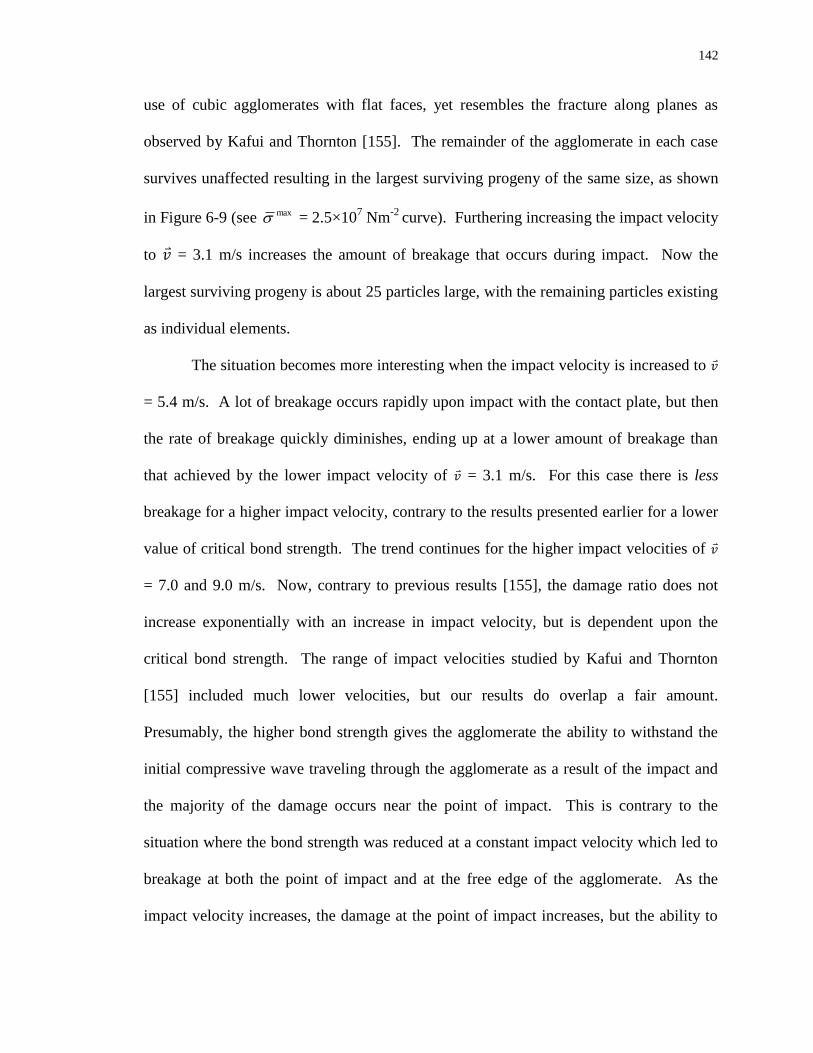
142

use of cubic agglomerates with flat faces, yet resembles the fracture along planes as

observed by Kafui and Thornton [155]. The remainder of the agglomerate in each case

survives unaffected resulting in the largest surviving progeny of the same size, as shown

in Figure 6-9 (see max = 2.5×107 Nm

-2 curve). Furthering increasing the impact velocity

to ⃑ = 3.1 m/s increases the amount of breakage that occurs during impact. Now the

largest surviving progeny is about 25 particles large, with the remaining particles existing

as individual elements.

The situation becomes more interesting when the impact velocity is increased to ⃑

= 5.4 m/s. A lot of breakage occurs rapidly upon impact with the contact plate, but then

the rate of breakage quickly diminishes, ending up at a lower amount of breakage than

that achieved by the lower impact velocity of ⃑ = 3.1 m/s. For this case there is less

breakage for a higher impact velocity, contrary to the results presented earlier for a lower

value of critical bond strength. The trend continues for the higher impact velocities of ⃑

= 7.0 and 9.0 m/s. Now, contrary to previous results [155], the damage ratio does not

increase exponentially with an increase in impact velocity, but is dependent upon the

critical bond strength. The range of impact velocities studied by Kafui and Thornton

[155] included much lower velocities, but our results do overlap a fair amount.

Presumably, the higher bond strength gives the agglomerate the ability to withstand the

initial compressive wave traveling through the agglomerate as a result of the impact and

the majority of the damage occurs near the point of impact. This is contrary to the

situation where the bond strength was reduced at a constant impact velocity which led to

breakage at both the point of impact and at the free edge of the agglomerate. As the

impact velocity increases, the damage at the point of impact increases, but the ability to

143

transfer the compressive wave into the rest of the agglomerate through the bonds is lost

because those particles experiencing the bulk of the force are no longer connected to the

agglomerate. Thus, their forces are non-transferrable and are converted into high

translational and rotational velocitiesIn effect, the particles broken off at the point of

impact act as buffers to shield the main agglomerate from forces that would otherwise

cause significant damage to the agglomerate. The high impact velocity decreases the

amount of time the agglomerate is near the point of contact essentially saving it from

potential breakage events. This behavior resembles the cushioning effect that occurs

when small particles shield larger particles from impacts in large scale mills, decreasing

the milling efficiency [8]. These results show that for this model increasing the energy of

impact does not always increase the amount of breakage and the particle parameters must

also be considered when designing such a breakage process. We are not aware of

experimental results showing this behavior, but we believe that the results we observe

make sense physically and may be observed with the right set of experiments.

The largest surviving progeny curve in Figure 6-9(b) matchs the behavior

described above. Starting at the lowest impact velocity, the primary progeny size

decreases from ⃑ = 1.0 and 2.2 m/s to ⃑ = 3.1 m/s. Then, a further increase in the impact

velocity to ⃑ = 5.4 m/s, then 7.0 m/s, then 9.0 m/s, increases the size of the primary

progeny surviving at the end of the breakage test, corresponding to the reduced extent of

overall breakage.

Additional values of critical bond strength were tested to further examine the

effect of impact velocity. Results from these tests are shown in Figure 6-10 for a

constant bond stiffness of nk = 1.0×109 Nm

-3. Each point on the plot is the final extent

144

of breakage extracted from the damage ratio plots for each run. For the lowest value of

critical bond strength ( max = 1.0×106 Nm

-3) all bonds are broken regardless of the

impact velocity. Increasing the critical bond strength to max = 1.0×107 Nm

-3 yields the

behavior discussed at the beginning of section 3.2, where the amount of breakage

increases with increasing impact velocity. Increasing the bond strength further ( max =

2.5×107 and 5.0×10

7 Nm

-3) yields the latter behavior discussed, where the maximum

amount of breakage is achieved at an intermediate impact velocity. At the highest value

of critical bond strength tested, max = 1.0×109 Nm

-3, there is no breakage at any of the

impact velocities tested. Interestingly, the maximum amount of breakage at the

intermediate levels of bond strength of max = 2.5×107 and 5.0×10

7 Nm

-3 occurs at a

different impact velocity for each value. In this figure, choosing an impact velocity and

increasing/decreasing the critical bond strength yields a monotonic trend in damage ratio.

As you increase (decrease) the critical bond strength, the amount of breakage or damage

ratio decreases (increases). If the chosen velocity is ⃑ = 3.1 m/s, you have the case

presented in the beginning of section 3.1. More work is needed to identify exactly what

determines the value of the optimum and why this optimum travels as the bond strength

is varied.

6.4 Effect of Particle Parameters

Our breakage investigation also included a study of the effect of common DEM

parameters on the breakage of agglomerates with the same bond parameters as the first

case discussed in this chapter, the base case with the parameters listed in Table 2-4 and

Table 2-5. The first investigation focused on the effect of the coefficient of restitution (

145

pe ), or the ratio of the post-collision velocity to the pre-collision velocity. Five different

values were tested, pe = 0.7, 0.1, 0.01, 0.001 and 0.0001 and results for the damage ratio

are shown in Figure 6-11. Generally, the behavior is very similar across all five cases,

post-collision velocity has little effect on the amount of breakage that occurs. Initially,

the damage ratio curves are virtually identical as the compressive wave travels through

the agglomerate causing similar fracture and particle detachment at the free edge of the

agglomerate. Below pe = 0.01, the influence of pe is minimal. Above that value you

get less breakage after the initial identical behavior. A possible explanation for this is that

at a high level of pe , those particles experiencing movement, yet not breakage, possess

sufficient energy after rebound to return to near their original positions within the

agglomerate. On the other hand, at a low level of pe , the particles lose the majority of

their energy and do not return to their original positions. The result is a deformed

agglomerate possessing already strained bonds that undergoes additional breakage as the

agglomerate rotates and rearranges after impact. Regardless, there is minimal difference

in the total amount of breakage between the cases with a high pe and a much lower pe .

Other combinations of stiffness and strength, producing almost complete breakage and

almost no breakage, show similar behavior, with the value of pe having only a minor

influence on the overall breakage observed. As breakage behavior does not vary

significantly with pe and the agglomerate deforms a fair amount after impact at lower

values of pe , we have used a realistic value for the coefficient of restitution for that of

glass reported in the literature, pe = 0.7 [173].

146

Two additional particle parameters were also varied, particle density ( ) and

Poisson’s ratio of the particles ( ). For both of these variables, little variation in

breakage behavior was observed for each of the three test cases (almost completely

broken, almost no breakage and intermediate breakage) over almost an order of

magnitude variation in the density ( = 1220 kgm-3

to 10,000 kgm-3

) and for Poisson’s

ratio varying from = 0.05 to 0.5. Therefore, the literature values for silica sand ( =

1220 kgm-3

and = 0.2) were selected and utilized for each of these parameters.

It is noted here that throughout the investigation the bulk of breakage products

consisted of a single primary progeny and many single, independent particles detached

from the original agglomerate. Never was a case found where the original agglomerate

was fractured into more than one fragment of intermediate size. It is proposed that this

was a result of a couple factors including the shape and regular structure of our

agglomerate, the limited resolution afforded when working with only 125 particles and a

limitation of this implementation of the model, where only a single value for each of the

bond parameters could be input. Real materials possess some distribution of strength due

to pre-existing flaws, grain boundaries, micro-cracks and heterogeneities which greatly

affects how stress is transmitted through the agglomerate. Kafui and Thornton [155]

suggest that “pre-existing flaws do not have a significant effect on agglomerate strength”,

yet the resolution of their spherical agglomerates was much finer than in our case.

Nonetheless, our work shines light on the nuances encountered when working with the

bonded particles model (BPM) similar to how Thornton [172] established the JKR theory

as a means to study agglomerate fracture.

147

6.5 Conclusion

Presented here is the use of the bonded particle model (BPM) within the

discrete element method (DEM) framework to investigate the breakage of agglomerates

composed of bonded spherical primary particles as a result of impact with an oblique

contact plate. Results show that the choice of bond parameters greatly affects the

breakage behavior, ranging from a completely broken agglomerate to a completely solid

agglomerate with less than two orders of magnitude difference in either the bond stiffness

or critical bond strength. Lower bounds on the bond stiffness were determined, below

which the material acts ductile, rather than the intended brittle fracture. In addition, an

agglomerate with more primary particles was simulated (1000 vs. 125), showing that the

smaller the primary particle size, the stronger the agglomerate.

When the impact velocity was varied, two different types of behavior were found.

At lower values of bond strength, the amount of breakage increased with increasing

impact velocity, matching the trends found in the literature. However, at higher values of

bond strength a maximum was achieved in the amount of breakage observed with an

increase in the impact velocity. We presume this was an effect of the detachment of

particles right at the point of impact acting as a buffer, shielding the remainder of the

agglomerate from the high velocity impact. This demonstrates that breakage is a highly

complex behavior that can vary greatly between multiple test conditions and even

models. Although we are not aware of experiments showing this behavior we believe the

results make sense physically and may be observed with the right set of experiments.

Investigations into the effect of common DEM parameters (coefficient of restitution,

148

density and Poisson’s ratio) did not demonstrate a significant effect on the breakage

behavior.

Yet to be identified is a means to achieve breakage similar to cleavage or massive

fracture, where progeny of a range of sizes are created. Increasing the agglomerate

resolution, incorporating bond strength and stiffness distributions, incorporating a

distribution in primary particle size and evaluating agglomerate shapes besides cubes are

all potential ways to vary the type of breakage away from disintegration and closer to

fracture. Further work is needed to investigate the effect of these approaches on the

Bonded Particle Model (BPM).

149

6.6 Figures for Chapter 6

Figure 6-1: Base case breakage over time: (a) 0.2 sec (b) 0.45 sec (c) 0.55 sec. Input parameters are

identical to those in Table 2-2 and Table 2-4.

Figure 6-2: High resolution imaging of an impact event. Particles are colored by their instantaneous

velocity, with the highest velocity red ( ⃑⃑⃑ = 4.1 m/s) and lowest blue ( ⃑⃑⃑ = 1.7 m/s). Identical simulation

conditions as Figure 6-1.

a b c

z

x

y

a b c

d e

t = 1.0 ms t = 6.9 ms t = 16.5 ms

t = 24.4 ms t = 39.4 ms

150

Figure 6-3: Breakage at 0.55 sec as a function of bond strength at a constant stiffness, nk = 1.0×109

Nm-3

. max = (a) 5.0×10

8 Nm

-2 (b) 1.0×10

8 Nm

-2 (c) 5.0×10

7 Nm

-2 (d) 2.5×10

7 Nm

-2 (e) 1.0×10

7 Nm

-2

(f) 1.0×106 Nm

-2. Instantaneous velocity of each particle is represented by its color ranging from the

lowest velocity of 0.56 m/s (blue) to the highest velocity of 3.8 m/s (red).

a b c

d e f

151

Figure 6-4: Damage ratio (fraction of original bonds broken) as a function of bond strength for those

cases shown in Figure 6-3, at a constant stiffness of nk = 1.0×109 Nm

-3.

-0.05

0.5

1.05

0.25 0.5 0.75

Time (s)

Da

ma

ge

Ra

tio

1.0x10

1.0x10

2.5x10

5.0x10

1.0x10

5.0x10

6

7

7

7

8

8

152

Figure 6-5: Largest surviving progeny as a function of bond strength at a constant stiffness of nk =

1.0×109 Nm

-3.

153

Figure 6-6: Breakage at 0.55 sec as a function of bond stiffness at a constant strength, max =

1.0×107 Nm

-2. nk = (a) 1.0×10

9 Nm

-3 (b) 5.0×10

8 Nm

-3 (c) 1.0×10

8 Nm

-3 (d) 5.0×10

7 Nm

-3. Particles are

colored according to their instantaneous velocity with the highest velocity of 4.2 m/s denoted by red

and the lowest velocity of 1.7 m/s denoted by blue.

a b

c d

154

Figure 6-7: Phase map of breakage types for various combinations of stiffness and strength. Blue

region (crosses) represents complete disintegration of the agglomerate. Green region (open squares)

represents no breakage of the agglomerate and yellow region (open circles) represents some, but not

complete, breakage of the agglomerate. Lower gray region represents the region of unrealistic

behavior.

155

Figure 6-8: Damage ratios for agglomerates with two different resolutions.

156

Figure 6-9: Largest surviving progeny as a function of impact velocity, at identical bond stiffness ( nk

= 1.0×109 Nm

-3) and different critical bond strengths,

max = 1.0×107

Nm-2

and max = 2.5×10

7 Nm

-

2.

0

25

50

75

100

125

0 5 10

Larg

est

Su

rviv

ing

Pro

gen

y

Impact Velocity (m/s)

1.0x10

2.5x10

7

7

157

Figure 6-10: Damage ratio (percentage of original bonds broken) as a function of impact velocity for

multiple bond strengths at a constant stiffness of nk = 1.0×109 Nm

-3.

0

0.5

1

0 5 10Impact Velocity (m/s)

Dam

ag

e R

ati

o1.0x10 1.0x10 2.5x10

5.0x10 1.0x10 1.0x10

6

7 8 9

7 7

158

Figure 6-11: Effect of coefficient of restitution (ep) on damage ratio at nk = 1.0×108 Nm

-3.

max =

5.0×106 Nm

-3.

0

0.5

1

0.1 0.3 0.5 0.7 0.9Time (s)

Dam

ag

e R

ati

oe = 0.7e = 0.1e = 0.01e = 0.001e = 0.0001p

p

p

p

p

159

Chapter 7 NUMERICAL EXAMINATION OF BREAKAGE IN A

BALL MILL

Despite the prevalence of ball milling in industry, little is known about how

varying the operational parameters of the mill (macroscopic parameters) affect the

breakage within the mill (microscopic behavior). Described in this chapter is the

implementation of the Bonded Particle Model (BPM) of Potyondy and Cundall [109]

within the Discrete Element Method (DEM) framework to analyze the breakage of

bonded agglomerates within a batch ball mill. The effect of mill operating parameters on

resultant breakage and flow profiles within the mill will be investigated, utilizing the

Attainable Region (AR) approach. The aim is to demonstrate that computational

simulation is a powerful tool for analyzing the flow and breakage in ball mills and can be

used as a decision-making tool for more efficient operation.

Agglomerates are formed following the same procedure as outlined in section

2.2.2 and implemented in Chapter 6, using the DEM approach overviewed in section

2.2.1. Each agglomerate is composed of 9 particles, instead of the 125 or 1000 of

Chapter 6. The geometry of the numerically simulated batch ball mill is presented in

section 2.2.3 and the variables of interest are identical to those investigated in the

experimental portion of this work (Chapter 4 and Chapter 5): rotation rate, grinding

media fill level, grinding media size and grinding time. In addition, the effect of bond

strength is also investigated.

160

7.1 Typical Behavior

Typical behavior of a ball mill simulation as a function of time is shown in Figure

7-1 for the base case simulation with max = 1.0×108 Nm

-2, J = 4.0%, md = 25.4 mm

and c = 0.53. Figure 7-1(a) shows the initial behavior of the mill (the majority of the

agglomerates are unbroken) at t = 0.7 seconds, with each color representing a quarter of

all agglomerates initially created in the simulation, i.e. each agglomerate (and thus the

primary particles within an agglomerate) was assigned a color initially and this color does

not change during the simulation. The remaining images shown in Figure 7-1 are after

eight complete revolutions, with each color representing a quarter of all agglomerates

initially created in the simulation. By this time in the simulation, the majority of the

agglomerates have been broken and do not resemble their initial shape. A range of sizes

and shapes can be seen, demonstrating that not only does significant breakage occur, but

the distribution suggests the simulations capture the irregularity of breakage observed in

experimental mills. As the lifters pass clockwise through the charge (Figure 7-1a and b),

they collect particles and raise the position of the charge (Figure 7-1c through e), until the

weight of the particles exceeds centrifugal force and the force of friction and the particles

crash back into the remainder of the charge (Figure 7-1f). It is apparent that, for this

parameter combination, both the agglomerates and the media are engaged by the passing

lifter, resulting in a cataracting motion (separation of the flow leaving the lifter from the

remainder of the charge) of each component of the charge.

The grinding mass fraction profiles corresponding to the simulation shown in

Figure 7-1 are plotted in Figure 7-2(a). At the beginning of the simulation, all of the

agglomerates reside in size class one, giving a mass fraction of M1 = 1. As rotation

161

commences, the agglomerates are broken and the mass fraction of the feed material

decreases and that of the intermediate size classes begins to increase. The intermediate

size classes achieve a maximum and then decrease as further revolution causes additional

breakage. The smallest size class, M4, constantly increases as its interval includes the

primary particle size. Eventually, the system should reach the state with M4 = 1 with the

mass fraction of all other size classes equal to zero.

Construction of the Attainable Region is straightforward once grinding profiles

similar to those shown in Figure 7-2(a) are available. In our system, the two fundamental

processes occurring are breakage and mixing. An idea of the objective function, or goals

of the optimization, helps to identify the key variables of interest. In this chapter, the

desired product is an intermediate size, as that situation necessitates breakage of the feed

material, but not complete breakage to the smallest size achievable in the mill. An

industrial example of such a scenario exists in the pharmaceutical industry where it is

desired to reduce the size of a drug to increase its surface area to volume ratio to increase

its bioavailability, but to simultaneously avoid fines, which pose inhalation risks to

personnel and present handling issues due to cohesion. Therefore, the first key variable

of interest is the amount of material in the intermediate size class, M2, and the source of

this material, the feed material (M1). Shown in Figure 7-2(b) is the physical construction

of the Attainable Region from the data in Figure 7-2(a). Begin by selecting a single

number of revolutions from the grinding profiles curve and draw a vertical line passing

through each of the grinding profiles (see Figure 7-2a). Select the intersection of this line

with the M1 curve as the x-coordinate and the intersection with the M2 curve as the y-

coordinate in M1-M2 phase space. This is represented by point E in Figure 7-2(b).

162

Repeat this process for each of the number of revolutions to develop the boundary of the

Attainable Region, starting at M1 = 1 and M2 = 0 and progressing towards the vertical

axis (see Figure 7-2b). The shaded region underneath this curve is referred to as the

Attainable Region because each and every point can be achieved by some combination of

milling and mixing. Finally, the desire is to produce the maximum amount of M2, so

operation would proceed until point M in Figure 7-2(b) was achieved, or about seven

drum revolutions. Additional runs can be introduced to this plot to easily perform

comparisons focusing only on those variables essential to the optimization problem. In

addition, construction of new Attainable Regions for different objective functions is

straightforward and will be described later in this chapter.

7.2 Effect of Critical Bond Strength

The first parametric investigation is to understand the effect the critical bond

strength max has on the flow and breakage in the batch ball mill simulation. Shown in

Figure 7-5 are snapshots of the flow at 10 revolutions for three different bond strengths,

max = 1.0×108 Nm

-2, 5.0×10

8 Nm

-2 and 1.0×10

9 Nm

-2, moving from left to right. Each

simulation is identical except for the critical strength of each bond. It is expected that the

lower the critical bond strength, the weaker the bonds, and the larger the extent of

breakage. Such a comparison would be similar to milling three different types of brittle

rock, each possessing different material strengths. Grinding profiles for the production of

the intermediate size product and the AR curves for each case are plotted in Figure 7-4.

One can see that the behavior, or lack thereof, observed in the snapshots is captured by

the AR plots and that the extent of breakage is very different for each of the cases. For

the lowest bond strength, there is significant breakage, whereas there is only minimal

163

breakage for the largest bond strength, resulting in a grinding profile always equal to zero

and an AR plot that does not change from its initial point of M1 = 1 and M2 = 0. There is

also only minor breakage for the intermediate level of critical bond strength, with its

grinding profile only departing slightly from zero and its AR curve only slightly

deviating from the initial agglomerate size distribution. It should be noted that 10

revolutions is a short length of operation for a ball mill, as the shortest run in the

equivalent experimental system was over 500 revolutions. Extended runs were

unfeasible due to the extreme computational expense of these simulations, such a run

requiring weeks-months of simulation. However, tuning material parameters is one way

to minimize run lengths, without sacrificing knowledge from the DEM approach.

In addition, the flow observed in Figure 7-3 is vastly different between the cases.

At the highest critical bond strength ( max = 1.0×109 Nm

-2), intact agglomerates are able

to stack on top of each other and reside on the lifter longer than the more broken

agglomerates at the lowest critical bond strength. As a result, the agglomerates (and

grinding media) follow a much longer trajectory after leaving the lifters and end their

flight near the toe of the load, whereas the components of the charge in the case of the

lowest critical bond strength make contact with the belly of the load and then roll towards

the toe.

This is seen better by following the motion of the grinding media. Shown in

Figure 7-5 are flow patterns, or orbits, traced by three representative grinding media from

each case, for 11.25 revolutions. Flow develops, untracked, for 1.8 revolutions (2

seconds of simulation time) to allow the grinding media profiles to develop complete

orbits, and then the locations of the representative grinding media are tracked for the

164

remainder of the simulation. The positions at uniformly spaced times are recorded and

then connected to develop the plots shown in Figure 7-5, with each color representing a

different grinding media. The more ballistic type trajectory for the case of stronger bonds

(see Figure 7-5c) produces an “eye” in the flow, where the particles that were once on the

lifter are separated from the remainder of the bed during flight. Such flow is termed

cataracting and rotation rate is often the variable controlling the flow regimes, not the

extent of breakage. The presence of the intact agglomerates on the lifters traps the

grinding media, holding them on the lifter longer, and thus giving them a larger orbit. On

the other hand, for the lowest critical bond strength (see Figure 7-5a), the grinding media

do not reside on the lifter for long, and fall off into the belly of the load. As a result, in

addition to the increased breakage due to reduced strength of the agglomerates, the

change in the grinding media orbit also contributes to the additional breakage observed.

This is one possible explanation of the steep increase in the extent of breakage with a

decrease in the bond strength of the agglomerate, i.e. there is minimal difference in flow

and breakage between max = 1.0×109 Nm

-2 and max = 5.0×10

8 Nm

-2, but a similar

decrease in the critical bond strength from max = 5.0×108 Nm

-2 to max = 1.0×10

8 Nm

-2

results in a large increase in the amount of breakage observed.

In order to further analyze the observed behavior we count contacts in the mill

(see Figure 7-6) in the following categories: grinding media with mill shell (GM-Shell),

grinding media with grinding media (GM-GM), grinding media with individual particles

(GM-Part), individual particles with the mill shell (Part-Shell) and individual particles

with each other (Part-Part). Quantifying the number of each type of contact occurring in

the mill offers support that the change in flow profiles as a result of increased breakage

165

increases those contacts promoting breakage. Shown in Figure 7-6 is the average number

of each type of contact occurring in the mill at each time step. The number of contacts

between the grinding media and the particles and the particles and the mill shell is scaled

by the total number of agglomerates in the system initially (200), whereas the number of

particle-particle contacts is scaled by the total number of particles (5400). For the two

cases with larger critical bond strength ( max = 1.0×109 Nm

-2 and max = 5.0×10

8 Nm

-2),

the distribution of contacts is similar for each type of contact. However, the case of the

lowest critical bond strength ( max = 1.0×108 Nm

-2) is quite different. Fewer inefficient

contacts between grinding media and grinding media and the mill shell occur, whereas

many more efficient grinding media and particle and particle and mill shell contacts

occur. Not every contact will produce breakage, but contacts between the grinding media

and the grinding media and the shell will never produce breakage, so decreasing the

occurrence of those contacts and increasing the occurrence of the efficient contacts

increases the likelihood of breakage. There is only a slight increase in the number of

particle-particle contacts between all cases as the critical bond strength is decreased.

Our results suggest that in the larger critical bond strength cases ( max = 1.0×109

Nm-2

and max = 5.0×108 Nm

-2), there are two sources of inefficiencies. First, the

excessive contacts between the grinding media and the grinding media and the mill shell

fail to convert the energy of rotation into the creation of new surface area. Second, the

efficient contacts that do occur are not energetic enough to cause fracture, and are thus

also energy sinks. An efficiently operating ball mill must thus monitor the flow of

grinding media to ensure that collisions are efficient (avoid contacts with the mill shell

and other grinding media) and energetic (cause fracture upon impact).

166

Also of interest is where the majority of breakage occurs within the mill. Figure

7-7 displays breakage event contour plots over the cross-section of the mill. The contour,

or frequency, plots are prepared by dividing the cross section into bins and recording the

number of breakage events that occur within that bin, then scaling by the total number of

breakage events. Breakage events are recorded over the length of the simulations,

including the initial settling period and the full length of each run (13 revolutions). These

plots support the previous results that the amount of breakage decreases as the critical

bond strength increases, almost vanishing for the highest case of bond strength tested.

However, the location of the breakage does not vary significantly between the cases.

Important to note here is the disparity in scales between each of the three cases, meant to

highlight the preferred breakage location in each case. The figure shows that the majority

of breakage happens near the mill shell, at the deepest point in the load. Thus, it is not

the agglomerates at the surface sustaining the initial contacts with the grinding media that

experience the majority of the breakage, but rather those that get away from the ballistic

impacts. Buchholtz et al [99] report similar results and explain that those particles

undergoing breakage are experiencing high compressive forces through force chain

networks.

Visual observation of the simulations suggests that as the grinding media crash

into the charge, they contact an intact agglomerate or group of particles on the surface

which does not break initially, but rebounds from the collision relatively unharmed. That

rebounding agglomerate continues to travel until it escapes the region of impact relatively

unharmed, or is trapped by the incoming grinding media and another agglomerate

beneath it. Movement of this pinned agglomerate along the mill shell is restricted, and

167

thus it is that agglomerate that experiences the majority of the breakage. The

agglomerate participating in the initial impact does experience some breakage, which is

captured by the region of intermediate breakage frequency above the region of extreme

breakage frequency near the mill shell in Figure 7-7(a). As a result, it appears that ball

mill efficiency is also dependent on the mobility of the bed, with a more confined bed

capable of more efficient conversion of applied energy into breakage.

7.3 Effect of Grinding Media Diameter

The next parameter investigated in this work is the effect of grinding media

diameter ( md ) at a constant grinding media fill level ( J ) and drum rotation rate ( c ) at

the lowest critical bond strength ( max = 1.0×108 Nm

-2). Snapshots of flow at 10

revolutions for different grinding media diameters are shown in Figure 7-8. Some

similarities exist with the situation where the critical bond strength was varied,

specifically the disparity in the extent of breakage between cases and the difference in

flow profiles as a result. For the smallest grinding media diameter, the agglomerates are

noticeably close to their original size, meaning that the grinding media do not deliver

sufficient energy to the agglomerates to cause significant breakage in the amount of time

simulated. Increasing the grinding media size makes a significant difference in the

amount of breakage observed. Similar to the case where the agglomerate bond strength

was large enough to prevent breakage (see Figure 7-3c), when operating with the smallest

grinding media size, the agglomerates stack on the passing lifter, and follow a large orbit

when they leave the lifter. Also, the smaller media are more easily taken up by the lifters

as the smaller diameter allows those particles to rest on the lifter longer as the lifter

passes through the bed. However, this drop height does not correlate to increased

168

breakage. At the two larger grinding media size, there is little noticeable difference in the

agglomerate flow behavior. There is obviously more breakage than the md = 12.7 mm

case (Figure 7-8a), but breakage in the the two larger media cases appears similar.

Looking at the grinding media profiles in Figure 7-9 tells a different story. These

orbits are tracked over 11 revolutions, after allowed 1.8 revolutions for the complete

orbits to develop, as explained before. As expected, the smaller media are able to follow

much longer orbits, reaching a higher level on the shoulder of the load and exhibiting an

“eye” similar to the case of the highest critical bond strength in Figure 7-5c. There is also

a fair amount of variation in the flow, from some media that follow long orbits to those

that seem trapped beneath the leading lifter and in front of the trailing lifter (see the red

orbit in Figure 7-9a). As the media diameter increases, the overall size of the orbits

decreases, but the variability also decreases, with the flow becoming more uniform. At

the highest diameter of grinding media, the flow profiles are restricted to a small orbit

near the mill shell. This is most likely because the lifters are not long enough to raise the

larger media, and the media fall off the rising lifter and roll down the free surface well

before the agglomerates and free primary particles do. These results are in agreement

with work by Djordjevic [67] who determined that lifter height has a significant influence

on flow within a ball mill.

Presented in Figure 7-12 are the average velocity field and granular temperature

(proportional to fluctuation velocity) for the grinding media for each size. The average

velocities are represented by the vectors and the granular temperature is shown by the

contours and calculated with the following:

'2

1umT

169

where 'u is the fluctuation velocity. It is important to note that the scales are not

equivalent for all cases, and the velocities and granular temperatures are generally an

order of magnitude lower for the case of the largest grinding media, compared to the

smallest grinding media. Therefore, as the grinding media size increases, the velocity of

the grinding media decreases. Average velocities correspond well with the grinding

media profiles shown in Figure 7-9. Granular temperature is a measure of the deviation

of individual particle velocity from the average particle movement in that area, with

regions of high granular temperature existing where particles have large fluctuations from

the mean velocity. Collisions between elements in the mill are discrete and often produce

a range of post-collisional velocities. Therefore, the areas of highest granular

temperature (red) can be interpreted as the region of frequent collision where the grinding

media conclude their ballistic trajectory and contact other elements of the flow. This

region is near the toe of the load for the md = 12.7 mm case, but shifts more towards the

interior of the flow as the grinding media diameter increases. Away from the toe of the

load in the md = 12.7 mm case the granular temperature is much lower, suggesting that

the remainder of the flow experiences solid body rotation, with little deviation from the

motion imparted by the mill shell and lifters. Also apparent from Figure 7-10 is the

influence of the size of the lifters on the flow profile, with the smallest media of a similar

size to the lifter height exhibiting a large orbit after leaving the passing lifter, which

progressively decreases and disappears for the largest media size investigated here.

Grinding media profiles for the intermediate, desired size class and the Attainable

Region curves for the three cases presented above are shown in Figure 7-11.

Corresponding to the behavior observed in Figure 7-8(a), the grinding media profiles and

170

the AR curve for the md = 12.7 mm case deviate only slightly from zero and from the

initial distribution of M1 = 1 and M2 = 0, respectively. This is in agreement with the

contention by Austin et al [63] that the grinding media ( md = 12.7 mm in our case)

should be larger than the feed particles ( Aggd = 14.4 mm in our case) to cause breakage.

For the other grinding media sizes, breakage is observed with the grinding profiles

passing through a maximum in the production of size class two. Initially, the two profiles

overlap, but begin to deviate around three drum revolutions or M2 = 0.3. By the time the

maximum amounts of M2 are reached, the larger diameter media produce about 13%

more of the desired product, with md = 25.4 mm achieving M2 = 0.46 at 7.25 revolutions

and md = 44.5 mm achieving M2 = 0.52 at ~5.5 revolutions.

Examining the contact distribution and spatial breakage distribution can help to

explain why the larger media produce more of the desired product. The average number

of contacts of each type per time step is shown in Figure 7-12. Since the number of

grinding media varies in each case, contacts with the grinding media have been scaled by

the number of grinding media in each case to provide a fair comparison. Scaling for the

other quantities is identical to before. For the case of the smallest media size investigated

( md = 12.7 mm), there are more contacts between the grinding media and each other, as

well as with the mill shell, relative to the other cases. The increased number of these

contacts is probably due to the greater amount of grinding media as the diameter is

decreased, increasing the probability that a grinding media is in the vicinity of another

grinding media. In addition, the larger orbit of the grinding media means that the

grinding media travel further after they leave the lifter, presumably having a higher

probability of contacting the particle lean toe of the load, increasing the chance of contact

171

with the mill shell. On the other hand, the number of contacts between the particles and

the mill shell for the smallest grinding media size is much smaller than for the other cases

( md = 25.4 mm and md = 44.5 mm). This is most likely because the majority of particles

are unbroken in the md = 12.7 mm case, so the mostly intact agglomerates pack

irregularly along the mill shell, minimizing the number of particles that actually contact

the mill shell. In addition, the diminished number of free primary particles means less

free particles are available to find their way through the voids and roll around in the

region behind the leading lifter and in front of the trailing lifter. The number of particle-

particle contacts is similar in each case, which is expected at a constant grinding media

fill level. The story is a little more complicated when looking at the two larger grinding

media sizes. The number of contacts between grinding media decreases because the

number of grinding media in the mill decreases, so it becomes less likely to find multiple

grinding media in the vicinity of each other. The number of contacts between grinding

media and particles decreases as you increase the grinding media diameter from md =

25.4 mm to md = 44.5 mm, which suggests that breakage should decrease, but the

opposite is true. Contrary to the md = 12.7 mm grinding media, the md = 25.4 mm

grinding media contact the agglomerates with sufficient energy to cause breakage as seen

by the AR profiles in Figure 7-11. As such, because there are more contacts between the

grinding media and the particles and the contacts possess sufficient energy to cause

breakage, more breakage is observed for the case of the intermediate grinding media size

than for the largest grinding media size investigated. What is meant by breakage here is

that for the same amount of particles broken from size class one (any point along the x-

axis in Figure 7-11b) there is less size class two, and thus more size class three, produced

172

for the intermediate size grinding media ( md = 25.4 mm). Additionally, interesting

behavior can be seen with the number of grinding media and mill shell contacts. There

are more grinding media-shell contacts in the largest diameter case, which may be a

result of the grinding media rolling down the free surface and reaching the particle-lean

toe of the load and then contacting the mill shell as seen in Figure 7-8(c). For the

intermediate grinding media size, there are a minimal number of contacts between the

grinding media and mill shell, whereas there is a larger proportion of contacts between

the grinding media and the particles. Therefore, the grinding media must flow off the

lifters into the material and not all the way to the mill shell, producing some breakage as

a result of the impact, as well as additional breakage from compressive forces near the

mill shell. Therefore, a reduction in the number of efficient contacts (grinding media-

particle) and an increase in the number of inefficient contacts (grinding media-shell),

results in a larger amount of the material of desired size, M2, for the largest size grinding

media ( md = 44.5 mm) compared to the intermediate grinding media ( md = 25.4 mm).

Spatial breakage distribution plots, shown in Figure 7-13, support this result.

Similar to the cases discussed earlier, the highest concentration of breakage events occurs

near the mill shell, for all cases. In addition, when comparing the breakage contours for

the two largest grinding media cases, the region below the center of the drum in the md =

44.5 mm case experiences less breakage than the md = 25.4 mm case. Throughout the

remainder of the cross-section, the breakage contours are very similar. The additional

breakage for the grinding media of intermediate size ( md = 25.4 mm) results in the

production of more size class three, making the intermediate size media less efficient at

producing the desired product, size class two. Two reasons are hypothesized for the

173

occurrence of this additional breakage, or overgrinding: 1) the general trajectory of the

grinding media impacts the belly of the load, increasing the occurrence of grinding

media-particle contacts and 2) the presence of the additional grinding media restricts the

movement of the agglomerates impacted by the grinding media, preventing them from

escaping, and resulting in additional breakage near the free surface of the charge. For the

case of the smallest grinding media, there is much less breakage, though it tends to occur

near the mill shell, consistent with previously discussed findings.

In an attempt to further explain why operation with the largest media produces

more of the intermediate sized product, the average kinetic energy of the grinding media

were calculated and are presented in Figure 7-14. Overlaid on top of the kinetic energy

contours are the average velocities identical to those in Figure 7-10. As mentioned

previously, the average velocity decreases as you increase the grinding media size, but

the kinetic energy increases. Therefore, the mass of the grinding media plays a much

bigger role than the grinding media velocity. Generally, the highest region of kinetic

energy is observed near the mill shell, but not where the majority of breakage occurs as

seen in Figure 7-13, especially for the two smaller media sizes. The overall kinetic

energy is least for the smallest grinding media, which corresponds to our contention that

the grinding media do not possess sufficient energy to cause significant breakage. An

increase in grinding media diameter corresponds to an increase in the average kinetic

energy of the grinding media. However, if this additional kinetic energy were consumed

in the form of increased impact energy with the agglomerates, one would expect

additional breakage, and thus a lower production of M2 and a higher production of M3 for

the largest grinding media diameter ( md = 44.5 mm). However, this is not the case, as

174

shown by the grinding media profiles and AR plots shown in Figure 7-11. We

hypothesize that the excess energy is consumed through inefficient collisions GM-Shell

contacts in the md = 44.5 mm which limit the amount of breakage experienced by the

agglomerates. As a result, there is not a direct correlation between the kinetic energy of

the grinding media and the production of a product of intermediate size. A full

characterization of the flow behavior and energy distribution is required to adequately

track the breakage in a batch ball mill. Overall, our results suggest that DEM simulations

are capable of capturing the effect of grinding media size on breakage in a batch ball mill,

which has been previously shown to a relevant parameter for ball mill performance [35,

55].

7.4 Effect of Grinding Media Fill Level

Plotted in Figure 7-15(a) are the grinding profiles of four different grinding media

fill levels ( J ) as a function of number of revolutions for the intermediate sized grinding

media ( md = 25.4 mm) and the lowest critical bond strength ( max = 1.0×108 Nm

-2) at a

constant rotation rate of c = 0.53. One can see that the number of revolutions (see

Figure 7-15a) required to achieve the maximum amount of size class two is similar for

the lower levels of grinding media fill, but is much less for the highest level of grinding

media ( J = 10.7%) Interestingly, there is little difference between the amount of size

class two produced with a single grinding media ( J = 0.3%) and the highest amount of

grinding media ( J = 10.7%). Operation with intermediate levels of grinding media ( J =

1.5% and J = 4.0%) yields slightly less of the desired size class two than the two

extreme cases. Though the two extreme levels may achieve approximately the same

175

maximum amount of M2, operation with J = 0.3% takes ~20% more revolutions to reach

that maximum (6.3 revolutions versus 5.4 revolutions). As a result, if time is also a

design constraint, it would be beneficial to operate at the higher grinding media fill level.

Such a requirement is common in the milling industry when it is desired to reduce the

size of starting material below a certain size as quickly as possible, i.e. at the highest

specific rate of breakage. Recommended levels of grinding media in these applications

are usually much larger than those investigated here ( J ~ 40% [35, 55]). Our results

support the idea that the specific rate of breakage increases as the grinding media fill

level increases away from its minimum value. Specifically, the rate of breakage

increases from 0.64 seconds-1

for J = 0.3% to ~0.68 seconds-1

for J = 1.5% and 4.0% to

1.21 seconds-1

for J = 10.7%, as calculated following the procedure outlined by King

[30] to determine the time-independent specific rate of breakage for batch grinding of

homogeneous solids. A straight line was fitted to the linear portion of the data once the

charge motion becomes steady, or after 2 complete revolutions. After the initial linear

period (~ 2-7 revolutions), the breakage rate accelerates as described by Bilgili and

Scarlett [8], most likely due to the increased frequency of efficient contacts as the

agglomerates break and flow begins to transition from the more dilated cataracting flow

to the more condensed cascading flow.

On the other hand, to optimize the production of an intermediate size class (our

objective function), a mill without grinding media can also yield a comparable amount of

the desired product. Implications of this suggest that, for relatively weak, brittle

materials, the contacts between the particles themselves and the particles and the mill

shell may be equally as efficient as contacts between the grinding media and the particles.

176

Therefore, the attention devoted to the effect of grinding media fill level in many design

equations may be unwarranted for a relatively weak material. AR plots for the four

different fill levels of grinding media (see Figure 7-15b) show that there is little

difference between breakage observed at each grinding media fill level. Despite the

difference in the time scales between the two extreme cases, their AR plots lie close to

one another, demonstrating that the conversion of the feed material to product is similar

in all cases.

Agglomerate/particle and grinding media flow profiles are similar between all of

the cases (not shown). The only difference is that as the fill level of grinding media

increases, the media begin to roll over one another, extending the width of the bed,

resulting in a higher load toe position. In addition, the general trends observed in the

number of contacts (not shown) are as expected. The number of contacts between the

grinding media, grinding media and mill shell and grinding media and particles increases

as the grinding media fill level increases. An explanation for this is that as the number of

grinding media increase, the chance of contact with other grinding media increases,

relative to the chance of contacting another element in the mill. The number of contacts

between the particles and the mill shell increases and the number of contacts between the

particles themselves decreases as you increase the grinding media fill level. This is most

likely a result of the increase in grinding rate as the grinding media fill level increases,

more readily producing single primary particles which are more likely to be in contact

with the mill shell than if they were still locked in the structure of an agglomerate.

177

7.5 Effect of Drum Rotation Rate

An essential variable to efficient ball mill operation is the drum rotation rate.

Snapshots of flow behavior at ten revolutions for three different rotation rates are shown

in Figure 7-16, with all other parameters held constant. The difference in the flow

behavior of the particles is vast, as expected. For the lowest drum rotation rate (see

Figure 7-16a), the lifters have a minimal effect on the flow and the particles basically

move together, other than a few particles near the shoulder that are raised a small amount

by the passing lifter. As a result, there is a large amount of intimate contacts between the

grinding media and the agglomerates. As the rotation rate increases, the lifters begin to

affect the flow more significantly, raising more particles to the previously established

shoulder of the flow (see Figure 7-16b). This causes a slight shift in the toe of the load

closer to the trailing lifter. However, the majority of the bed still resides in a small cross

section of the drum. Increasing the rotation rate even further (see Figure 7-16c) leads to

the regime previously discussed, where the majority of the particles and the grinding

media are taken airborne before they crash into the bed. Now the particles are much

more spread out across the drum cross section

Similar behavior is seen with the grinding media profiles shown in Figure 7-17,

for 9.0 revolutions in Figure 7-17(a), 10.7 revolutions in Figure 7-17(b) and 11.25

revolutions in Figure 7-17(c). The numbers of revolutions vary because as the rotation

rate decreases, the computational expense increases, and the slower runs were cut short to

facilitate the analysis. As before, these figures were drawn by allowing the orbits to fully

develop over 1.8 revolutions before the positions of 3 representative grinding media were

tracked for the remainder of the simulation. The two lower rotation rates show similar

178

patterns of flow, with the grinding media exhibiting closed orbits close to the mill shell,

and not rising to the level of the previously established shoulder. Only the particles are

affected by the lifters at low rotation rates, and the grinding media flow profiles do not

vary significantly, except for a lower shoulder for the lowest rotation rate. At a higher

rotation rate, the lifters are able to capture the grinding media as they pass through the

flow, sending the grinding media airborne, and thus increasing the size of the grinding

media orbits

The plot of the average number of contacts between each of the elements (Figure

7-18) tells us a lot about what is going on inside the mill. In general, there are more

contacts between all elements for the lowest rotation rate. This makes sense because the

flow in Figure 7-16(a) is limited to the smallest cross section, meaning that there is a

higher probability of contact between each particle, the grinding media and the mill shell.

For the lowest rotation rate, all particles roll down the free surface once they reach the

shoulder of the load, and the smaller particles and agglomerates percolate into the bed

and continually deny the larger media from penetrating the belly of the charge.

Therefore, the grinding media traverse the entire length of the free surface and contact the

mill shell before they are reincorporated into the solid body rotation. As the rotation rate

is increased, the flow dilates some as a result of the increased action of the lifters,

allowing some of the grinding media to penetrate the belly of the load, decreasing the

amount of grinding media that reach the toe of the load, and thus decreasing the number

of grinding media-mill shell contacts. In addition, the lifters act more strongly on some

of the larger remaining particles, displacing them to the toe of the load, which prevents

contact between the grinding media flowing on the surface and the mill shell. These two

179

factors contribute to the large decrease in the number of GM-Shell contacts between the

lowest rotation rate ( c = 0.10) and the two larger rotation rates ( c = 0.30 and 0.53).

The number of GM-GM contacts is similar between each of the cases, but interestingly

there are the most for the intermediate rotation rate. For the highest rotation rate ( c =

0.53), the number of GM-GM contacts are reduced because the flow is more spread out

along the cross-section of the drum. Therefore, as each case contains the same number of

grinding media, the probability of two grinding media contacting each other is reduced.

As for the number of GM-Part, Part-Shell and Part-Part contacts, the differences in the

charge flow are responsible for the decrease in each as the rotation rate increases. The

smaller flow cross section means that the particles are more densely packed, increasing

the number of sustained contacts. The increased number of airborne particles in the

larger rotation rate cases decreases the number that are residing near the mill shell, as

thus decreases the number of particle-mill shell contacts.

Grinding profiles for the three rotation rates are shown in Figure 7-19(a). The

profiles for c = 0.10 and c = 0.30 follow each other very closely until about three

revolutions, when they begin to deviate, and the c = 0.30 case achieves a maximum

amount of size class two of M2 = 0.49. However, the case of c = 0.53 does not follow

the initial trajectory of the other two curves and does not produces M2 as efficiently as the

other two. The charge profiles in Figure 7-16 suggest that as the rotation rate increases,

the size of the orbit of the charge also increases. Thus, we can assume that as the

particles become more ballistic, their collisions with the bed become less efficient at

breakage, which is supported by the fact that a lower maximum of M2 is obtained at a

larger number of revolutions than the lower rotation rate of c = 0.30. The maximum

180

amount of M2 produced at the slowest rotation rate is lower than that at the intermediate

rotation rate because the increased number of collisions (of all types as shown in Figure

7-18) results in increased breakage that quickly breaks particles into and out of the

desired particle size class. The Attainable Region plots for this case (Figure 7-19b)

demonstrate similar behavior. From this presentation it is easy to see that the c = 0.30

case yields the most of the desired product and that all three curves initially overlap until

M1 ~ 0.6, indicating that the conversion of feed material to desired product is initially

similar for all three rotation rates.

Grinding media profiles for the two lower rotation rates up until the point of

deviation of the grinding profiles (~ 3 revolutions) are presented in Figure 7-20.

Surprisingly, though the grinding profiles and Attainable Region curves are almost

identical (see Figure 7-19), the grinding media profiles are quite different. The profiles in

Figure 7-20 are not at steady-state and include both transient (1.8 revolutions) and some

steady state operation (1.2 revolutions), and are thus not identical to the similar plots in

Figure 7-17. For a rotation rate of c = 0.30, the flow is more dilated, which

differs from the steady state flow shown in Figure 7-17(b). Flow in the c = 0.10 case is

similar in both the transient and steady state regime, with a slightly lower shoulder of the

load in the steady-state orbit (see Figure 7-17a). These results suggest that there is not a

unique correlation between flow and resultant breakage, and just because the breakage is

similar does not imply identical flow. Thus, a true understanding of breakage dynamics

must also include a description of the internal flow dynamics. Our results show that the

cases of c = 0.10 and c = 0.30 have greater breakage rates than the c = 0.53 case.

181

This is different from the traditional design suggestions that ball mills should be operated

at about c = 0.70 to increase the specific rate of breakage [35, 55].

Traditional design equations rarely include the size of the grinding media ( md ),

but almost always include the amount of grinding media ( J ) [55]. In the results

presented in this chapter we observe that the grinding media size plays an important role

in the production of a product of intermediate size, whereas the grinding media fill level

has a relatively small effect. Caution is advised though, as results presented here are for a

limited set of parameters and more work is needed to obtain general trends. However, it

should be noted that the experiments presented in Chapter 4 and Chapter 5 and in recent

experimental and numerical works [174, 175] show that the size of the grinding media

can affect breakage dynamics.

7.6 Optimal Production of Size Class Three

Until now the Attainable Region has been a convenient way to compare multiple

runs, but the same information could be determined from the grinding profiles versus

number of revolutions. In addition, we have focused on the feed material (size class one,

M1) and the material just smaller than the feed (size class two, M2 – see Table 2-6).

Presented below is an additional optimization using the AR analysis, demonstrating the

ability to extend the AR through mixing, the other fundamental process occurring in the

mill. Consider the situation where it is desired to achieve a product particle size

distribution consisting of greater than 15% of a smaller, yet still intermediate sized

product (size class three, M3 – see Table 2-6) with more than 20% of the original material

(size class one, M1) remaining in the product. Such a situation is encountered in

industries where increased surface area of the smaller particles is desired, e.g. the

182

pharmaceutical industry where the bioavailability of an active pharmaceutical ingredient

is inversely proportional to the particle size and when processing coal to fire power

plants, where smaller particles provide a more consistent burn. However, often a

decrease in particle size leads to handling difficulties, so it is desired to retain some

material in a larger size class. Shown in Figure 7-21 is an optimization of such a process

using the AR, where the key variables of interest are now M3, the smaller intermediate

sized product, and M1, the original feed material. The plot in Figure 7-21(a) for c =

0.53 starts at M1 = 1 and M3 = 0, and then proceeds towards M1 = 0 and M3 = 1. Similar

behavior is seen for the c = 0.10 and c = 0.30 curves in Figure 7-21(a). However, it

does so following a trajectory that increases in slope as it approaches its maximum value

of M3. This is because M1 is first broken into size class two, resulting in a slow M3

production rate, which then increases as M2 achieves a maximum and those particles are

broken into size class three. The result is a concave boundary of the Attainable Region,

which will be exploited later. The same set of data used to create Figure 7-19 was used

to construct the curves shown in Figure 7-21(a), the only difference being the choice of

key variables, which correlate directly to those specified by the constraint. No new

simulations were required to handle the change of constraint/objective function. Figure

7-21(b) shows the milling AR as well as the region that satisfies the new constraint of M3

> 0.15 and M1 > 0.20. Notice that there is no intersection between the two regions, so it

would appear that the current milling conditions cannot produce the required material.

However, one of the characteristic features of the Attainable Region approach is the

ability to fill in concave regions with the use of mixing rules. In the phase space

presentation of the Attainable Region, mixing two species is represented by a straight line

183

connecting the two conditions. If one were to draw a line connecting the point

representing the feed (point F in Figure 7-21c) with the point representing the maximum

amount of M3 produced at these parameters combinations (point M ), any point under the

line MF (shaded purple region in Figure 7-21c) can be achieved through mixing.

Combining the previous AR with this extension constructs the new, now completely

convex AR, as shown in Figure 7-21(d). Now there exists a point of intersection between

the region specifying the constraint and the AR, (point S in Figure 7-21d). This point is

obtained by operating the mill to point M, then mixing the mill outlet concentration with

additional feed material, similar to feed bypass encountered when optimizing networks of

chemical reactions (see Chapter 3). Specifically, the proportions of each state to be

mixed are obtained according to the Lever Arm Rule [169]. The distance of MS relative

to MF determines the contribution of feed material to the final mixture. For example,

MS is 18% of the distance MF , so point S is obtained by mixing 18% feed material

with 82% material from point M . Following the procedure outlined above enables a

simple and straightforward determination of the ability of a process to obtain desired

targets, and to quantify the operation that achieves these desired distributions.

These simulations were based on the series of batch ball mill experiments

presented in Chapter 4 and Chapter 5, which showed that grinding media size plays an

important role in the breakage behavior. This numerical work replicated the trends that

the most amount of the desired material (size class two, M2) was achieved using the

largest grinding media size tested ( md = 44.5 mm in both the experiments and the

simulations). In addition, an intermediate rotation rate achieved the most amount of the

desired product for some of the conditions tested in both the experimental and the

184

simulation work. Finally, the Attainable Region (AR) analysis was utilized to establish a

procedure to achieve a product size distribution that was not achievable through only the

milling conditions investigated. This agreement lends legitimacy to using bonded

agglomerates within the DEM framework to approximate the breakage of brittle

materials, despite the fact that size of the agglomerates utilized in the simulations was

larger than the mono-size feed utilized in the experiments. Also, breakage was only

observed to follow the abrasion or attrition mechanism, and massive fracture and

cleavage were not observed. Such a limitation of our model is concerning, but the ability

to reproduce shapes of the breakage and Attainable Region profiles is encouraging and

suggests that abrasion may play a more significant role than initially anticipated in batch

ball mill operation. More work is needed to investigate the effect of bond parameters in

larger systems ball mill systems. Finally, relatively weak agglomerates were simulated in

order to minimize the computational expense, yet still capture and analyze breakage.

Hence, it is unknown if stronger agglomerates processed for longer run times will exhibit

similar trends. Further work is required in this direction as computing power continues to

advance.

7.7 Conclusion

Presented here is the use of the Bonded Particle Model (BPM) within the Discrete

Element Method (DEM) framework to analyze the breakage of brittle materials in a batch

ball mill. The investigation utilized the Attainable Region (AR) approach to determine

the effect of critical bond strength ( max ), grinding media diameter ( md ), grinding media

fill level ( J ) and drum rotation rate ( c ) on flow and breakage of bonded agglomerates.

It was observed that breakage occurs predominantly at the deepest point in the charge,

185

closest to the mill shell, and not at the point of impact between the grinding media and

the mill charge. Grinding media diameter ( md ) affected the breakage in the mill,

exhibiting little breakage for grinding media below the agglomerate size and extensive

breakage for grinding media sizes greater than twice the size of the agglomerate. In

addition, an intermediate grinding media size of md = 25.4 mm exhibited more breakage

than a grinding media size of md = 44.5 mm at otherwise identical parameters, most

likely due to the increase in number of contacts occurring between the grinding media

and the material as a result of the variations in the grinding media flow profiles. In our

work, the effect of grinding media fill level ( J ) was found to not be as important a factor

as historically suggested in the milling literature, producing similar amounts of a desired

product of intermediate size for a range of grinding media fill levels from J = 0.3% to J

= 10.7%. However, the specific rate of breakage increased as the level of grinding media

increased, matching previously reported trends at these low levels of grinding media fill

[35]. Traditional mill design equations rarely include the size of the grinding media but

routinely include the amount of grinding media. Our results show that the size of the

grinding media can be an important factor as has been shown in Chapter 5 and other

recent experiments [174, 175]. An intermediate drum rotation rate ( c = 0.30) was found

to produce the most amount of the desired product, in agreement with experimental

results from Chapter 5 where the optimum was also an intermediate rotation rate. At the

lowest rotation rate of c = 0.10, there are a large number of contacts between all

elements in the mill, yielding the most breakage observed. At the highest rotation rate

investigated ( c = 0.53), the nature of the contacts with the grinding media shifts from

contacts with the material to contacts with each other and the mill shell, reducing the

186

efficiency of conversion of rotational energy to breakage energy. The intermediate

rotation rate exists as a balance between these two cases, promoting efficient contacts

between the grinding media and the particles, but not encouraging excessive contacts

between all elements to drive the system away from optimal production of the

intermediate size product. Finally, a situation was presented demonstrating the power of

the Attainable Region to optimize processes with a constraint.

Results from this investigation suggest that variation of operating parameters is a

potential avenue to increase the energy efficiency of ball milling operations, specifically

to tune grinding media sizes and fill levels, along with drum rotation rates to encourage

contacts that may lead to breakage and minimize those that waste input energy to

inefficient contacts between grinding media and grinding media and the mill shell. The

results in this work are for a limited set of parameters and operating conditions so it

remains to be seen if the same trends would be observed for other systems. Extensions of

this work are currently underway to continue to explore the parameter space and shrink

the agglomerate size to more realistically approximate the granular elements in

experimental ball mills.

187

7.8 Figures for Chapter 7

Figure 7-1: Snapshots of flow at different times for the base case: c = 0.53, max = 1.0×10

8 Nm

-2,

md = 25.4 mm and J = 4%. t = (a) 0.7 s (b) 9.1 s (c) 9.2 s (d) 9.3 s (e) 9.4 s (f) 9.5 s. Flow patterns

repeat approximately every 0.5 seconds. Grinding media are colored grey.

Figure 7-2: Construction of the Attainable Region for the base case simulation: c = 0.53, max =

1.0×108 Nm

-2, md = 25.4 mm and J = 4%. (a) Grinding profiles as a function of number of

revolutions (b) Attainable Region.

b

c d

a b c

d e f

0

0.1

0.2

0.3

0.4

0.5

0 0.2 0.4 0.6 0.8 1M 1

M2

0

0.5

1

0 5 10Revolutions

Mass F

racti

on

MMMM

1

2

3

4 E

b a M

188

Figure 7-3: Snapshots of flow at 10 revolutions for various bond strengths (max ) at a rotation rate

of c = 0.53, J = 4%, md = 25.4 mm. max = (a) 1.0×10

8 Nm

-2 (b) 5.0×10

8 Nm

-2 (c) 1.0×10

9 Nm

-2.

Each color represents 25% percent of the agglomerates originally created.

Figure 7-4: Construction of the Attainable Region for variation in bond strength: c = 0.53, J = 4%

and md = 25.4 mm. (a) Grinding profiles as a function of number of revolutions (b) Attainable

Region.

Figure 7-5: Grinding media flow profiles for various bond strengths (max ) at a rotation rate of c

= 0.53, J = 4%, md = 25.4 mm. max = (a) 1.0×10

8 Nm

-2 (b) 5.0×10

8 Nm

-2 (c) 1.0×10

9 Nm

-2. Colors

correspond to three different representative grinding media.

a b c

0

0.1

0.2

0.3

0.4

0.5

0 0.2 0.4 0.6 0.8 1M 1

M2

1.0x105.0x101.0x10

9

0

0.1

0.2

0.3

0.4

0.5

0 4 8 12Revolutions

M2

1.0x105.0x101.0x10

8

8

9

8

8 b a

-0.1 -0.05 0 0.05 0.1-0.1

-0.05

0

0.05

0.1

Y (m)

Z (

m)

-0.1 -0.05 0 0.05 0.1-0.1

-0.05

0

0.05

0.1

Y (m)

Z (

m)

-0.1 -0.05 0 0.05 0.1-0.1

-0.05

0

0.05

0.1

Y (m)

Z (

m)

a b c

X (m) X (m) X (m)

Z (

m)

189

Figure 7-6: Average number of contacts per time step between the grinding media and the mill shell,

the other grinding media and the individual particles as a function of critical bond strength. GM-

Part* and Part-Shell* are scaled by the number of agglomerates present in the system initially (200)

and Part-Part* is scaled by the total number of particles in the system (5400).

Figure 7-7: Breakage event density map for various bond strengths (max ) at a rotation rate of c =

0.53, J = 4%, md = 25.4 mm. max = (a) 1.0×10

8 Nm

-2 (b) 5.0×10

8 Nm

-2 (c) 1.0×10

9 Nm

-2. Color

denotes frequency of breakage events and the scale is different for each figure.

0.0

1.0

2.0

3.0

4.0

5.0

GM-Shell GM-GM GM-Part* Part-Shell* Part-Part*

Avg N

um

ber

of

Con

tacts

1.0x10

5.0x10

1.0x10

8

8

9

a b c

X (m) X (m) X (m)

Z (

m)

190

Figure 7-8: Snapshots of flow at 10 revolutions for various grinding media sizes at a critical bond

strength of 1.0×108 Nm

-2, c ~ 0.53 and J = 4%. md = (a) 12.7 mm (b) 25.4 mm (c) 44.5 mm. Each

color represents 25% percent of the agglomerates originally created.

Figure 7-9: Grinding media profiles for various grinding media sizes at a critical bond strength of

1.0×108 Nm

-2, c ~ 0.53 and J = 4%. md = (a) 12.7 mm (b) 25.4 mm (c) 44.5 mm. Colors correspond

to three different representative grinding media.

Figure 7-10: Velocity maps for various grinding media sizes at a critical bond strength of 1.0×108

Nm-2

, c ~ 0.53 and J = 4%. md = (a) 12.7 mm (b) 25.4 mm (c) 44.5 mm. Vectors represent average

grinding media velocity and color denotes fluctuation velocity of grinding media.

a b c

-0.1 -0.05 0 0.05 0.1-0.1

-0.05

0

0.05

0.1

Y (m)

Z (

m)

-0.1 -0.05 0 0.05 0.1-0.1

-0.05

0

0.05

0.1

Y (m)

Z (

m)

a b c

-0.1 -0.05 0 0.05 0.1-0.1

-0.05

0

0.05

0.1

Y (m)

Z (

m)

Z (

m)

X (m) X (m) X (m)

a b c

Z (

m)

X (m) X (m) X (m)

191

Figure 7-11: Construction of the Attainable Region for variation in grinding media diameter: max

= 1.0×108 Nm

-2, c = 0.53 and J = 4%. (a) Grinding profiles as a function of number of revolutions

(b) Attainable Region.

Figure 7-12: Average number of contacts per time step between the grinding media, the mill shell

and the individual particles as a function of critical bond strength. GM-Shell* and GM-GM* area

scaled by the number of grinding media in each case. GM-Part* and Part-Shell* are scaled by the

number of agglomerates present in the system initially (200) and Part-Part* is scaled by the total

number of particles in the system (5400).

0

0.1

0.2

0.3

0.4

0.5

0.6

0 0.2 0.4 0.6 0.8 1M 1

M2

d = 12.7 mm d = 25.4 mmd = 44.5 mm

0

0.1

0.2

0.3

0.4

0.5

0.6

0 4 8 12Revolutions

M2

d = 12.7 mm d = 25.4 mmd = 44.5 mm

m

m

m

m

m

m

b a

0.0

2.5

5.0

GM-Shell* GM-GM* GM-Part* Part-Shell* Part-Part*

Avg

Nu

mb

er

of

Co

nta

cts d = 12.7mm

d = 25.4mm

d = 44.5mm

m

m

m

192

Figure 7-13: Breakage event density map for various grinding media sizes at a critical bond strength

of 1.0×108 Nm

-2, c ~ 0.53 and J = 4%. md = (a) 12.7 mm (b) 25.4 mm (c) 44.5 mm. Color denotes

frequency of breakage events.

Figure 7-14: Kinetic energy contours for various grinding media sizes at a critical bond strength of

1.0×108 Nm

-2, c ~ 0.53 and J = 4%. md = (a) 12.7 mm (b) 25.4 mm (c) 44.5 mm. Color denotes

kinetic energy of grinding media in mJ.

a b c Z

(m

)

X (m) X (m) X (m)

a b c

Z (

m)

X (m) X (m) X (m)

193

Figure 7-15: Construction of the Attainable Region for variation in grinding media fill level: max =

1.0×108 Nm

-2, c = 0.53 and md = 25.4 mm. (a) Grinding profiles as a function of number of

revolutions (b) Attainable Region.

Figure 7-16: Snapshots of flow at 10 revolutions for various rotation rates (RPM) with max =

1.0×108 Nm

-2, md = 25.4 mm and J = 4%. c = (a) 0.10 (b) 0.30 (c) 0.53. Each color represents

25% percent of the agglomerates originally created.

Figure 7-17: Grinding media profiles for various rotation rates (RPM) with max = 1.0×10

8 Nm

-2,

md = 25.4 mm and J = 4%. c = (a) 0.10 (b) 0.30 (c) 0.53. Colors correspond to three different

representative grinding media.

0

0.1

0.2

0.3

0.4

0.5

0.6

0 0.2 0.4 0.6 0.8 1M 1

M2

J = 0.3%J = 1.5%J = 4.0%J = 10.7%

0

0.1

0.2

0.3

0.4

0.5

0.6

0 4 8 12Revolutions

M2

J = 0.3%J = 1.5%J = 4%J = 10.7%

b a

a b c

-0.1 -0.05 0 0.05 0.1-0.1

-0.05

0

0.05

0.1

Y (m)

Z (

m)

-0.1 -0.05 0 0.05 0.1-0.1

-0.05

0

0.05

0.1

Y (m)

Z (

m)

-0.1 -0.05 0 0.05 0.1-0.1

-0.05

0

0.05

0.1

Y (m)

Z (

m)

a b c

Z (

m)

X (m) X (m) X (m)

194

Figure 7-18: Average number of contacts per time step between the grinding media and the mill

shell, the other grinding media and the individual particles as a function of critical bond strength.

GM-Part* and Part-Shell* are scaled by the number of agglomerates present in the system initially

(200) and Part-Part* is scaled by the total number of particles in the system (5400).

Figure 7-19: Construction of the Attainable Region for variation in drum rotation rate: max =

1.0×108 Nm

-2, J = 4% and md = 25.4 mm. (a) Grinding profiles as a function of number of

revolutions (b) Attainable Region.

0.0

2.0

4.0

6.0

GM-Shell GM-GM GM-Part* Part-Shell* Part-Part*

Avg N

um

ber

of C

onta

cts 0.10

0.30

0.53

c

c

c

0

0.1

0.2

0.3

0.4

0.5

0.6

0 0.2 0.4 0.6 0.8 1M 1

M2

0.10 0.30 0.53

0

0.1

0.2

0.3

0.4

0.5

0.6

0 4 8 12Revolutions

M2

0.10 0.30 0.53

c

c

c

c

c

c b a

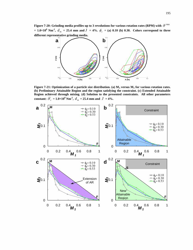
195

Figure 7-20: Grinding media profiles up to 3 revolutions for various rotation rates (RPM) with max

= 1.0×108 Nm

-2, md = 25.4 mm and J = 4%. c = (a) 0.10 (b) 0.30. Colors correspond to three

different representative grinding media.

Figure 7-21: Optimization of a particle size distribution. (a) M3 versus M1 for various rotation rates.

(b) Preliminary Attainable Region and the region satisfying the constraint. (c) Extended Attainable

Region achieved through mixing. (d) Solution to the presented constraints. All other parameters

constant: c = 1.0×108 Nm

-2, md = 25.4 mm and J = 4%.

-0.1 -0.05 0 0.05 0.1-0.1

-0.05

0

0.05

0.1

Y (m)

Z (

m)

-0.1 -0.05 0 0.05 0.1-0.1

-0.05

0

0.05

0.1

Y (m)

Z (

m)

a b

Z (

m)

Z (

m)

X (m) X (m)

0

0.1

0.2

0 0.2 0.4 0.6 0.8 1M 1

M3 0.10

0.30 0.53

0

0.1

0.2

0 0.2 0.4 0.6 0.8 1M 1

M3

0.10 0.30 0.53

0

0.1

0.2

0 0.2 0.4 0.6 0.8 1M 1

M3

0.10 0.30 0.53

0

0.1

0.2

0 0.2 0.4 0.6 0.8 1M 1

M3

0.10 0.30 0.53

c

c

c

c

c

c

c

c

c

c

c

c

F

M

Attainable Region

M

F

S

Constraint

Constraint

New Attainable

Region

Extension of AR

M

F

a b

c d

196

Chapter 8 CONCLUSIONS AND FUTURE WORK

8.1 Conclusions

Presented here is a computational and experimental investigation of the flow and

breakage of particles in a batch ball mill consisting of a horizontally rotating cylinder

filled with steel grinding media and material to be reduced in size. The effect of grinding

media fill level, grinding media diameter and drum rotation rate on particle breakage and

flow was studied in both an experimental batch ball mill and computational

representation of the same, in addition to a numerical investigation as to how particle

strength influences operation. In general, operational parameters significantly affect flow

and breakage behavior, and there is potential to tune these parameters to increase the

efficiency of ball milling. Throughout this work, the goal has been to optimize the

production of a product of intermediate size. This has been accomplished using a tool

originally developed for analysis of complex chemical reaction networks called the

Attainable Region (AR) analysis, which has been demonstrated to be a powerful tool for

the optimization of size reduction processes. We have attempted to address some of the

gaps in knowledge of why ball milling is so inefficient, how particles break under an

applied force and to elucidate the most important variables affecting ball mill operation.

This work will contribute to the development of optimal policies to efficiently break

particles from bench to industrial scale and to identify critical process parameters,

ultimately enabling better control of product particle size distribution and the

development of more sophisticated size reduction technologies.

197

Our investigation began with the characterization of breakage in an experimental

ball mill. A range of breakage behavior was measured for variations in both the drum

rotation rate and the level of grinding media. Our objective was to produce the greatest

amount of an intermediate sized product from the feed material, while minimizing the

production of undesired fines. Using the Attainable Region (AR) analysis, it was shown

that the lowest achievable level of grinding media at the lowest drum rotational speed

achievable with our equipment yielded the most amount of the desired product. At

higher levels of grinding media fill level, breakage curves lay on top of one another,

presumably because the excess energy input from frequent collisions with the grinding

media hindered the ability to selectively produce only the desired product. At lower fill

levels, these collisions were far less frequent, enabling the drum rotation rate to control

the extent of breakage. A significant drawback of operation at the lowest rotation rate

and grinding media fill level was the time required to achieve the optimal amount of

desired product. Experimental manipulations of the rotation rate partway through the run

were able to produce close to the target, single speed optimal, requiring less than 50% of

the original run length. Such operation is similar to placing two mills in series operating

at different levels of energy input, validating the potential of this approach to recommend

optimal policies at the industrial scale.

Extension of this idea was made to operation with smaller grinding media. No

longer did the optimal parameter combination reside on the boundary of the parameter

space, but intermediate levels of both the grinding media fill level and the drum rotation

rate yielded the most of the desired product of intermediate size when operating with the

smaller media. We speculate that at the lowest parameter combination each collision

198

between the grinding media and the particles does not have sufficient energy to cause

breakage 100% of the time, and thus a threshold for breakage has been reached. This

enables one to use both drum rotation rate and grinding media fill level as control

variables to encourage or repress breakage, depending on the particular desires of the

process. However, the champion for production of an intermediate sized product

remained the lowest combination of grinding media fill level and drum rotation rate with

the larger grinding media. Nevertheless, grinding media size has been demonstrated to

be an important parameter for ball mill operation, though it is rarely incorporated into

design and scale-up equations.

Numerical investigations were pursued to delve into the behavior outlined above

in an attempt to explain the breakage and flow behavior on the particle level. Initial

analysis was performed by incorporating of the Bonded Particle Model (BPM) into the

Discrete Element Method (DEM) framework to study the breakage resulting from

dropping agglomerates from a prescribed height onto a contact plate. Agglomerates were

formed by approximating larger particles with groups of spheres, connected by

collections of springs representing bonds between elements. The strength of the bonds

was varied, demonstrating a range of breakage from agglomerates that disintegrated

completely upon impact at low bond strengths, to those that remained unaffected by the

impact at high bond strengths, to a range of breakage for those of intermediate bond

strength. Increasing the stiffness of the bonds caused a transition in the breakage from

agglomerates that underwent elastic deformation as the bonds stretched, but then returned

to their original positions, to agglomerates that disintegrated upon impact due to the

inability of the bonds between each particle to stretch. Higher resolution agglomerates of

199

the same dimensions but more primary particles experience less breakage at otherwise

identical conditions, and thus behave as if they are stronger. Breakage behavior is

linearly proportional to impact velocity for low impact velocities and a range of bond

strengths and stiffnesses. At higher impact velocities, particles near the point of impact

with the contact plate detach from the agglomerate and act as buffers, shielding the

remainder of the agglomerate from significant damage. Variation of standard DEM input

parameters ( pe , and ) exhibited little effect on the overall breakage behavior.

Modeling breakage with this implementation of the BPM was unable to reproduce

breakage following the cleavage or massive fracture mechanism, partly, we hypothesize,

because of the lack of bond strength distribution and partly, we hypothesize, because of

the lack of agglomerate shape and distribution. Nevertheless, our examination revealed

the complex sensitivity of agglomerate breakage to bonding and test parameters, and our

results can be used to avoid improper bond parameter selection to produce realistic

breakage.

Knowledge gained about the breakage of single particles was extended to

simulations of multiple agglomerates in a numerical batch ball mill approximating that

used in the experimental investigations. The presence of many agglomerates allows one

to follow the evolution of particle size distributions as a function of simulation and

operational parameters. As expected, agglomerate bond strength was found to

significantly affect the extent of breakage, but it also had a major influence on the charge

flow profiles. Good agreement was observed with the experimental trends that the larger

media tested yield more of an intermediate sized product. The number of contacts

between the grinding media and the agglomerates increases as the grinding media

200

diameter decreases, more quickly breaking agglomerates into and out of the desired

product size range. However, little variation in the extent of breakage was observed with

an increase in grinding media fill level, somewhat surprising since grinding media fill

level is such a prominent component of the most frequently referenced scale-up and

design equations. However, the specific rate of breakage was found to increase with an

increase in the grinding media fill level. An intermediate rotation rate produces the most

of the desired product at a constant grinding media diameter, because a balance exists

between a large number of contacts at the lower rotation rate that quickly create and

destroy the desired product and the fewer number of contacts at the higher rotation rate,

where efficient contacts occur less frequently. Breakage was found to occur

predominantly near the mill shell and not at the charge surface where the grinding media

contact the material. Charge flow affects how media contact the charge and thus whether

energy is converted into either efficient of inefficient contacts. At least for the case of

relatively weak particles, it has been demonstrated that tuning operational parameters to

promote efficient contacts is a realistic means to increase the efficiency of ball milling,

and there is potential benefit in altering flow conditions as the run proceeds since charge

flow varies as the extent of breakage increases.

We have found that the influence of grinding media diameter cannot be ignored

when investigating the operation of ball mills. In addition, charge flow profiles may be

as important as the amount of energy that is intended to be delivered to the material.

Addition of media does not correlate to more of a desired intermediate product, but

efficient contacts must be encouraged to convert the energy delivered by the media into

particle breakage. This requires knowledge of how flow profiles are affected by

201

operating parameters and the extent of breakage occurring in a mill. It is crucial for scale

up and design equations to include all parameters, combining time dependent material

parameters that vary with the extent of breakage, operational parameters that control

flow, e.g. rotation rate, and those that control the energy transferred from drum rotation to

particle breakage – grinding media size and grinding media fill level. Generally,

experimental trends were matched by the computational approach, encouraging

implementation of this approach as a future test bed for various particle breakage

operations. Thus, we have illustrated the promise of using BPM as part of the DEM

framework to determine basic breakage trends and provide preliminary recommendations

for optimal policies before extensive experimentation is performed.

8.2 Future Work

Real materials are characterized by slight variations in size, shape, strength,

composition, etc. However, the current implementation of the BPM in the DEM

framework only enables a distribution of properties for the primary particles, and bond

parameters are limited to a single value. Future investigations should develop the model

to incorporate a distribution of bond parameters, as then one would expect to capture

breakage following all three main breakage mechanisms – abrasion, cleavage and

massive fracture. As a result, distinguishing between breakage mechanisms would

facilitate the ability to promote breakage following the more efficient mechanism. One

way to do this is to include unbreakable elements of varying size and shape that are

bonded together to represent a heterogeneous composite material [81, 152]. This creates

a rock sample with non-uniform distributions of voids and internal friction, as well as

202

irregular grain boundaries. Thus, applied forces are not distributed evenly through the

sample and fracture becomes more realistic.

In addition, intuitive extensions of the present work may provide additional

valuable information. Such extensions include longer simulations with stronger

agglomerates to compare breakage and flow on timescales similar to the experiments and

decreasing the primary particle size to approach the size ratio between grinding media

and the particles in the experiments. Methods to increase the amount of information

available from DEM simulations with breakage without significant increase in

computational expense have been presented, including extrapolating results from a mill

slice to the entire mill [82]. Continuing to explore the parameter space of the

experimental system is also warranted. Extensions to additional grinding media sizes,

grinding media fill levels and rotation rates within and outside the ranges presented may

also be of interest.

Results discussed here are focused on dry ball milling, but wet ball milling is also

an important operation in many industries. In particular, nanosizing of particles for

pharmaceutical products in stirred media mills is a promising approach as drug

candidates become more complex and less soluble [11]. Introducing an interstitial fluid

is possible by coupling a computational fluid dynamics (CFD) package with the DEM

framework. Initial investigations could begin at the current scale, and decrease to

approach the nanosizing scale. One simplification that can be made on the nanosizing

scale is to track the motion of only the grinding media, similar to Reichardt and Weichert

[77]. Incorporating breakage at this scale is challenging due to the extreme number of

particles present, yet the basic modeling approach is similar. One emerging wet milling

203

technology is stirred media milling, relevant for ultrafine grinding in both the

pharmaceutical industry [11] and the minerals processing industry [176]. The simulation

and analysis tools presented here are robust enough to study the behavior inside such a

mill as well as correlate mill operating parameters with product particle size distributions

in order to optimize its operation.

In additional to extending the work to different types of ball milling, this approach

is relevant to other types of milling as well. This work has focused on batch ball milling,

but the same basic approach can be taken to analyze resultant particle size distributions

from continuously operated mills. An example of such a mill is the pin mill, which is

commonly used in the pharmaceutical industry to reduce the size of drug crystals [177].

Changing mill rotation rate is similar to feeding material from one mill operating at one

set of parameters to another mill operating at another set of conditions. Residence time

can replace batch time to correlate the amount of time a representative amount of material

resides in each milling environment to the amount of breakage it undergoes, but

otherwise the Attainable Region analysis is unchanged. Such an investigation is

attractive to address the needs of most solids handling industries, as most processes

involving size reduction operate continuously.

Finally, Population Balance Modeling (PBM) is a promising approach to

modeling breakage (and agglomeration) processes [39], yet developing breakage kernels

is still in its infancy [178]. Knowledge and data of breakage from the current study can

be provided to the PBM framework to develop a unified analysis tool to predict resultant

particle size distributions given a description of the material, geometry and operating

204

conditions. Ultimately, this approach could be used as smart decision making and design

tool to increase the efficiency of particle breakage operations.

205

REFERENCES

1. Müller, F. and R.F. Polke, From the product and process requirements to the milling facility.

Powder Technology, 1999. 105(1-3): p. 2-13.

2. Morrison, R.D. and P.W. Cleary, The road towards a Virtual Comminution Machine, in

DEM072007: Brisbane, Australia. p. 1-12.

3. Fuerstenau, D.W. and A.Z.M. Abouzeid, The energy efficiency of ball milling in comminution.

International Journal of Mineral Processing, 2002. 67(1-4): p. 161-185.

4. Shelley, S., Preventing Dust Explosions. Chemical Engineering Progress, 2008. 104(3): p. 8-14.

5. Ghadiri, M. and Z. Zhang, Impact attrition of particulate solids. Part 1: A theoretical model of

chipping. Chemical Engineering Science, 2002. 57(17): p. 3659-3669.

6. Roche, O., M.A. Gilbertson, J.C. Phillips, and R.S.J. Sparks, The influence of particle size on the

flow of initially fluidised powders. Powder Technology, 2006. 166(3): p. 167-174.

7. Abou-Chakra, H. and U. Tüzün, Microstructural blending of coal to enhance flowability. Powder

Technology, 2000. 111(3): p. 200-209.

8. Bilgili, E. and B. Scarlett, Population balance modeling of non-linear effects in milling processes.

Powder Technology, 2005. 153(1): p. 59-71.

9. Bilgili, E., On the consequences of non-first-order breakage kinetics in comminution processes:

Absence of self-similar size spectra. Particle & Particle Systems Characterization, 2007. 24(1): p.

12-17.

10. Florence, A.T., E.G. Salole, and J.B. Stenlake, The effect of particle size reduction on digoxin

crystal properties. Journal of Pharmacy and Pharmacology, 1974. 26: p. 479-480.

11. Merisko-Liversidge, E., G.G. Liversidge, and E.R. Cooper, Nanosizing: a formulation approach

for poorly-water-soluble compounds. European Journal of Pharmaceutical Sciences, 2003. 18(2):

p. 113-120.

12. Elan, Technology Focus: Helping you bring products to market, 2007.

13. Otsuka, M., K. Otsuka, and N. Kaneniwa, Relation Between Polymorphic Transformation

Pathway During Grinding and the Physicochemical Properties of Bulk Powders for

Pharmaceutical Preparations. Drug Development and Industrial Pharmacy, 1994. 20(9): p. 1649 -

1660.

14. Varinot, C., S. Hiltgun, M.-N. Pons, and J. Dodds, Identification of the fragmentation mechanisms

in wet-phase fine grinding in a stirred bead mill. Chemical Engineering Science, 1997. 52(20): p.

3605-3612.

15. Lynch, A.J., Mineral Crushing and Grinding Circuits1977, New York: Elsevier. 342.

16. Rubinstein, M.H. and P. Gould, Particle Size Reduction in the Ball Mill. Drug Development and

Industrial Pharmacy, 1987. 13(1): p. 81-92.

17. Bwalya, M.M., M.H. Moys, and A.L. Hinde, The use of the discrete element method and fracture

mechanics to improve grinding rate prediction. Minerals Engineering, 2001. 14(6): p. 565-573.

18. Bond, F.C., Crushing & Grinding Calculations, Part I. British Chemical Engineering, 1961. 6(6):

p. 378-385.

19. Potapov, A.V., C.S. Campbell, and M.A. Hopkins, A Two-Dimensional Dynamic Simulation of

Solid Fracture Part II: Examples. International Journal of Modern Physics C, 1995. 6(3): p. 399-

425.

20. Kendall, K., The impossibility of comminuting small particles by compression. Nature, 1978.

272(5655): p. 710-711.

21. Marshall, V.C., Comminution1974, London: IChemE.

22. Mishra, B.K., A review of computer simulation of tumbling mills by the discrete element method:

Part I--contact mechanics. International Journal of Mineral Processing, 2003. 71(1-4): p. 73-93.

23. Venugopal, R. and R.K. Rajamani, 3D simulation of charge motion in tumbling mills by the

discrete element method. Powder Technology, 2001. 115(2): p. 157-166.

24. Bridgwater, J., The dynamics of granular materials - towards grasping the fundamentals. Granular

Matter, 2003. 4(4): p. 175-181.

25. Lowrison, G.C., Crushing and grinding : the size reduction of solid materials1974, Cleveland,

Ohio: CRC Press. viii, 286 p.

206

26. Austin, L.G., A commentary on the Kick, Bond and Rittinger laws of grinding. Powder

Technology, 1973. 7(6): p. 315-317.

27. Rittinger, P.R.v., Lehrbuch der Aufbereitungs Kunde1867, Berlin: Ernst and Korn.

28. Kick, F., Das Gesetz der Proportionalem Widerstand und Seine Anwendung1885, Leipzig: Felix.

29. Bond, F.C., Crushing & Grinding Calculations, Part II. British Chemical Engineering, 1961. 6(6):

p. 543-548.

30. King, R.P., Modeling and Simulation of Mineral Processing Systems2001, Boston: Butterworth

Heinemann.

31. Morrell, S., An alternative energy-size relationship to that proposed by Bond for the design and

optimisation of grinding circuits. International Journal of Mineral Processing, 2004. 74(1-4): p.

133-141.

32. Austin, L.G., Introduction to the mathematical description of grinding as a rate process. Powder

Technology, 1971. 5(1): p. 1-17.

33. Teng, S., P. Wang, L. Zhu, M.-W. Young, and C.G. Gogos, Mathematical modeling of fluid

energy milling based on a stochastic approach. Chemical Engineering Science, 2010. 65(15): p.

4323-4331.

34. Baxter, J., A. Abu-Nahar, and U. Tuzun, The breakage matrix approach to inadvertent particulate

degradation: dealing with intra-mixture interactions. Powder Technology, 2004. 143-4: p. 174-

178.

35. Ozkan, A., M. Yekeler, and M. Calkaya, Kinetics of fine wet grinding of zeolite in a steel ball mill

in comparison to dry grinding. International Journal of Mineral Processing, 2009. 90(1-4): p. 67-

73.

36. Bazin, C. and G. Lavoie, Ball-mill rotation speed and rate of particle breakage: results for a full-

scale unit. Mineral Processing & Extractive Metallurgy: Transactions of the Institution of Mining

& Metallurgy, Section C, 2000. 109(3): p. 161-164.

37. Varinot, C., H. Berthiaux, and J. Dodds, Prediction of the product size distribution in associations

of stirred bead mills. Powder Technology, 1999. 105(1-3): p. 228-236.

38. Free, K.S., M.K. McCarter, and R.P. King, Evaluation of a new method for work index estimation

using single particle impact tests, in SME Annual Meeting2004: Denver, CO.

39. Herbst, J.A. and D.W. Fuerstenau, Scale-up procedure for continuous grinding mill design using

population balance models. International Journal of Mineral Processing, 1980. 7(1): p. 1-31.

40. Kelly, E.G. and D.J. Spottiswood, The breakage function; What is it really? Minerals Engineering,

1990. 3(5): p. 405-414.

41. Bilgili, E., J. Yepes, and B. Scarlett, Formulation of a non-linear framework for population

balance modeling of batch grinding: Beyond first-order kinetics. Chemical Engineering Science,

2006. 61(1): p. 33-44.

42. Bilgili, E., R. Hamey, and B. Scarlett, Nano-milling of pigment agglomerates using a wet stirred

media mill: Elucidation of the kinetics and breakage mechanisms. Chemical Engineering Science,

2006. 61(1): p. 149-157.

43. Mishra, B.K., A review of computer simulation of tumbling mills by the discrete element method:

Part II--Practical applications. International Journal of Mineral Processing, 2003. 71(1-4): p. 95-

112.

44. Bernotat, S. and K. Schonert, Size Reduction, in Ullman's Encyclopedia of Industrial Chemistry

B21988.

45. Gao, M.-W. and E. Forssberg, A study on the effect of parameters in stirred ball milling.

International Journal of Mineral Processing, 1993. 37(1-2): p. 45-59.

46. Djordjevic, N., R. Morrison, B. Loveday, and P. Cleary, Modelling comminution patterns within a

pilot scale AG/SAG mill. Minerals Engineering, 2006. 19(15): p. 1505-1516.

47. Alexander, A., F.J. Muzzio, and T. Shinbrot, Effects of scale and inertia on granular banding

segregation. Granular Matter, 2004. 5(4): p. 171-175.

48. Hill, K.M. and J. Kakalios, Reversible axial segregation of rotating granular media. Physical

Review E, 1995. 52(4): p. 4393.

49. Arntz, M.M.H.D., W.K.d. Otter, W.J. Briels, P.J.T. Bussmann, H.H. Beeftink, and R.M. Boom,

Granular mixing and segregation in a horizontal rotating drum: A simulation study on the impact

of rotational speed and fill level. AIChE Journal, 2008. 54(12): p. 3133-3146.

207

50. McCarthy, J.J., T. Shinbrot, G. Metcalfe, J.E. Wolf, and J.M. Ottino, Mixing of granular materials

in slowly rotated containers. AIChE Journal, 1996. 42(12): p. 3351-3363.

51. Hill, K.M., G. Gioia, and D. Amaravadi, Radial Segregation Patterns in Rotating Granular

Mixtures: Waviness Selection. Physical Review Letters, 2004. 93(22): p. 224301.

52. Agrawala, S., R.K. Rajamani, P. Songfack, and B.K. Mishra, Mechanics of media motion in

tumbling mills with 3d discrete element method. Minerals Engineering, 1997. 10(2): p. 215-227.

53. Potapov, A.V. and C.S. Campbell, The breakage induced by a single grinding ball dropped onto a

randomly packed particle bed. Powder Technology, 2000. 107(1-2): p. 108-117.

54. Boateng, A.A. and P.V. Barr, Modelling of particle mixing and segregation in the transverse

plane of a rotary kiln. Chemical Engineering Science, 1996. 51(17): p. 4167-4181.

55. Austin, L.G., R.R. Klimpel, and P.T. Luckie, Process Engineering of Size Reduction: Ball

Milling1984, New York: American Institute of Mining, Metallurgical, and Petroleum Engineers,

Inc.

56. Iwasaki, T., J.H. Kim, and M. Satoh, Characterization of media mills based on mechanical energy

applied to particles. Chemical Engineering Science, 2006. 61(4): p. 1065-1073.

57. Arentzen, C. and R. Bhappu, High Efficiency Ball Mill Grinding. Engineering and Mining Journal,

2008. 209(3): p. 62-4,66,68.

58. Cleary, P.W., Predicting charge motion, power draw, segregation and wear in ball mills using

discrete element methods. Minerals Engineering, 1998. 11(11): p. 1061-1080.

59. Shoji, K., S. Lohrasb, and L.G. Austin, The variation of breakage parameters with ball and

powder loading in dry ball milling. Powder Technology, 1980. 25(1): p. 109-114.

60. Yokoyama, T., K. Tamura, H. Usui, and G. Jimbo, Simulation of ball behavior in a vibration mill

in relation with its grinding rate: effects of fractional ball filling and liquid viscosity. International

Journal of Mineral Processing, 1996. 44-45: p. 413-424.

61. Fahrenwald, A.W., Why a Smaller Ball Load Gives Better Milling Economy. Engineering and

Mining Journal, 1954. 155: p. 79.

62. Erdem, A.S. and S.L. Ergün, The effect of ball size on breakage rate parameter in a pilot scale

ball mill. Minerals Engineering, 2009. 22(7-8): p. 660-664.

63. Austin, L.G., K. Shoji, and P.T. Luckie, The effect of ball size on mill performance. Powder

Technology, 1976. 14(1): p. 71-79.

64. Shoji, K., L.G. Austin, F. Smaila, K. Brame, and P.T. Luckie, Further studies of ball and powder

filling effects in ball milling. Powder Technology, 1982. 31(1): p. 121-126.

65. Cundall, P.A. and O.D.L. Strack, A discrete numerical model for granular assemblies.

Geotechnique, 1979. 29(1): p. 47-65.

66. Cleary, P.W. and D. Hoyer, Centrifugal mill charge motion and power draw: comparison of DEM

predictions with experiment. International Journal of Mineral Processing, 2000. 59(2): p. 131-148.

67. Djordjevic, N., Discrete element modelling of the influence of lifters on power draw of tumbling

mills. Minerals Engineering, 2003. 16(4): p. 331-336.

68. Feng, Y.T., K. Han, and D.R.J. Owen, Discrete element simulation of the dynamics of high energy

planetary ball milling processes. Materials Science and Engineering a-Structural Materials

Properties Microstructure and Processing, 2004. 375-77: p. 815-819.

69. Morrison, R.D. and P.W. Cleary, The road towards a Virtual Comminution Machine, in 4th

International Conference on DEM2007: Brisbane, Australia. p. 1-12.

70. Potapov, A.V. and C.S. Campbell, The two mechanisms of particle impact breakage and the

velocity effect. Powder Technology, 1997. 93(1): p. 13-21.

71. Potapov, A.V. and C.S. Campbell, Computer simulation of impact-induced particle breakage.

Powder Technology, 1994. 81(3): p. 207-216.

72. Rajamani, R.K., P. Songfack, and B.K. Mishra, Impact energy spectra of tumbling mills. Powder

Technology, 2000. 108(2-3): p. 116-121.

73. Abd El-Rahman, M.K., B.K. Mishra, and R.K. Rajamani, Industrial tumbling mill power

prediction using the discrete element method. Minerals Engineering, 2001. 14(10): p. 1321-1328.

74. Morrison, R.D., P.W. Cleary, and M.D. Sinnott, Using DEM to compare the energy efficiency of

pilot scale ball and tower mills. Minerals Engineering, 2009. 22(7-8): p. 665-672.

75. Potapov, A.V. and C.S. Campbell, Computer simulation of shear-induced particle attrition.

Powder Technology, 1997. 94(2): p. 109-122.

208

76. Seyedi Hosseininia, E. and A.A. Mirghasemi, Numerical simulation of breakage of two-

dimensional polygon-shaped particles using discrete element method. Powder Technology, 2006.

166(2): p. 100-112.

77. Reichardt, R. and W. Wiechert, Event driven algorithms applied to a high energy ball mill

simulation. Granular Matter, 2007. 9(3): p. 251-266.

78. Inoue, T. and K. Okaya, Grinding mechanism of centrifugal mills -- a simulation study based on

the discrete element method. International Journal of Mineral Processing, 1996. 44-45: p. 425-435.

79. Chen, X.-s., Q. Li, and S.-m. Fei, Constrained model predictive control in ball mill grinding

process. Powder Technology, 2008. 186(1): p. 31-39.

80. Inoue, T., K. Okaya, S. Owada, and T. Homma, Development of a centrifugal mill -- a chain of

simulation, equipment design and model validation. Powder Technology, 1999. 105(1-3): p. 342-

350.

81. Cheng, Y.P., Y. Nakata, and M.D. Bolton, Discrete element simulation of crushable soil.

Geotechnique, 2003. 53(7): p. 633-641.

82. Cleary, P.W., Recent advances in DEM modelling of tumbling mills. Minerals Engineering, 2001.

14(10): p. 1295-1319.

83. Morrison, R.D. and P.W. Cleary, Using DEM to model ore breakage within a pilot scale SAG mill.

Minerals Engineering, 2004. 17(11-12): p. 1117-1124.

84. Herbst, J.A. and A.V. Potapov, Making a Discrete Grain Breakage model practical for

comminution equipment performance simulation. Powder Technology, 2004. 143-144: p. 144-150.

85. Tomiczek, K., Modeling of sandstone rock samples using PFC2D code, in Numerical Modeling in

Micromechanics via Particle Methods, H. Konietzky, Editor 2003, Swets & Zeitlinger: Lisse, The

Netherlands.

86. Mishra, B.K. and C.V.R. Murty, On the determination of contact parameters for realistic DEM

simulations of ball mills. Powder Technology, 2001. 115(3): p. 290-297.

87. Mishra, B.K. and R.K. Rajamani, The discrete element method for the simulation of ball mills.

Applied Mathematical Modelling, 1992. 16(11): p. 598-604.

88. Dong, H. and M.H. Moys, Assessment of discrete element method for one ball bouncing in a

grinding mill. International Journal of Mineral Processing, 2002. 65(3-4): p. 213-226.

89. Misra, A. and J. Cheung, Particle motion and energy distribution in tumbling ball mills. Powder

Technology, 1999. 105(1-3): p. 222-227.

90. van Nierop, M.A., G. Glover, A.L. Hinde, and M.H. Moys, A discrete element method

investigation of the charge motion and power draw of an experimental two-dimensional mill.

International Journal of Mineral Processing, 2001. 61(2): p. 77-92.

91. Mishra, B.K. and R.K. Rajamani, Simulation of charge motion in ball mills. Part 2: numerical

simulations. International Journal of Mineral Processing, 1994. 40(3-4): p. 187-197.

92. Tavares, L.M. and R.P. King, Single-particle fracture under impact loading. International Journal

of Mineral Processing, 1998. 54(1): p. 1-28.

93. Refahi, A., J. Aghazadeh Mohandesi, and B. Rezai, Discrete element modeling for predicting

breakage behavior and fracture energy of a single particle in a jaw crusher. International Journal

of Mineral Processing, 2010. 94(1-2): p. 83-91.

94. Salman, A.D. and D.A. Gorham. The fracture of glass spheres under impact loading. in Powders

& Grains 97. 1997. Rotterdam: Balkema.

95. Mishra, B.K. and C. Thornton, Impact breakage of particle agglomerates. International Journal of

Mineral Processing, 2001. 61(4): p. 225-239.

96. Ning, Z., R. Boerefijn, M. Ghadiri, and C. Thornton. Effects of particle size and bond strength on

impact breakage of weak agglomerates. in Powders & Grains 97. 1997. Rotterdam: Balkema.

97. Liu, L., K.D. Kafui, and C. Thornton, Impact breakage of spherical, cuboidal and cylindrical

agglomerates. Powder Technology, 2010. 199(2): p. 189-196.

98. Potapov, A.V. and C.S. Campbell, Parametric dependence of particle breakage mechanisms.

Powder Technology, 2001. 120(3): p. 164-174.

99. Buchholtz, V., J.A. Freund, and T. Poschel, Molecular dynamics of comminution in ball mills.

European Physical Journal B, 2000. 16(1): p. 169-182.

100. Dolgunin, V.N., A.N. Kudy, and A.A. Ukolov, Development of the model of segregation of

particles undergoing granular flow down an inclined chute. Powder Technology, 1998. 96(3): p.

211-218.

209

101. Rosato, A., K.J. Strandburg, F. Prinz, and R.H. Swendsen, Why the Brazil nuts are on top: Size

segregation of particulate matter by shaking. Physical Review Letters, 1987. 58(10): p. 1038.

102. Metzger, M.J., B. Remy, and B.J. Glasser, All the Brazil nuts are not on top: Vibration induced

granular size segregation of binary, ternary and multi-sized mixtures. Powder Technology, 2011.

205(1-3): p. 42-51.

103. Conway, S.L., X. Liu, and B.J. Glasser, Instability-induced clustering and segregation in high-

shear Couette flows of model granular materials. Chemical Engineering Science, 2006. 61(19): p.

6404-6423.

104. Lawrence, L.R. and J.K. Beddow, Powder segregation during die filling. Powder Technology,

1969. 2(5): p. 253-259.

105. McElwaine, J. and K. Nishimura, Size Segregations in Snow Avalanches, in IUTAM Symposium

on Segregation in Granular Flows, A.D. Rosato and D.L. Blackmore, Editors. 1999, Kluwer

Academic Publishers: Cape May, NJ. p. 81-88.

106. Jain, N., J.M. Ottino, and R.M. Lueptow, Combined size and density segregation and mixing in

noncircular tumblers. Physical Review E (Statistical, Nonlinear, and Soft Matter Physics), 2005.

71(5): p. 051301-10.

107. Nityanand, N., B. Manley, and H. Henein, An analysis of radial segregation for different sized

spherical solids in rotary cylinders. Metallurgical and Materials Transactions B, 1983. 17(2): p.

247-257.

108. Fakhimi, A., J.J. Riedel, and J.F. Labuz, Shear Banding in Sandstone: Physical and Numerical

Studies. International Journal of Geomechanics, 2006. 6(3): p. 185-194.

109. Potyondy, D.O. and P.A. Cundall, A bonded-particle model for rock. International Journal of Rock

Mechanics and Mining Sciences, 2004. 41(8): p. 1329-1364.

110. Shinbrot, T. and F.J. Muzzio, Nonequilibrium Patterns in Granular Mixing and Segregation.

Physics Today, 2000. 53(3): p. 25-30.

111. Nordell, L.K., A.V. Potapov, and J.A. Herbst. Comminution Simulation Using Discrete Element

Method (DEM) Approach - From Single Particle Breakage to Full-Scale SAG Mill Operation. in

SAG. 2001. Vancouver, BC.

112. Herbst, J.A., A microscale look at tumbling mill scale-up using high fidelity simulation.

International Journal of Mineral Processing, 2004. 74(Supplement 1): p. S299-S306.

113. Tusar, M., L. Tusar, and J. Zupan, The optimisation of energy consumption and time in colour

pigment grinding with pearl mills. Journal of Materials Processing Technology, 2006. 171(1): p.

48-60.

114. Zhang, F.L., M. Zhu, and C.Y. Wang, Parameters optimization in the planetary ball milling of

nanostructured tungsten carbide/cobalt powder. International Journal of Refractory Metals and

Hard Materials, 2008. 26(4): p. 329-333.

115. Hou, T.-H., C.-H. Su, and W.-L. Liu, Parameters optimization of a nano-particle wet milling

process using the Taguchi method, response surface method and genetic algorithm. Powder

Technology, 2007. 173(3): p. 153-162.

116. Su, C.-H. and T.-H. Hou, Using multi-population intelligent genetic algorithm to find the pareto-

optimal parameters for a nano-particle milling process. Expert Systems with Applications, 2008.

34(4): p. 2502-2510.

117. Herbst, J.A. and Y.C. Lo, Financial implications of comminution system optimization.

International Journal of Mineral Processing, 1996. 44-45: p. 209-221.

118. Wibowo, C. and K.M. Ng, Operational issues in solids processing plants: Systems view. AIChE

Journal, 2001. 47(1): p. 107-125.

119. Jankovic, A., W. Valery, and E. Davis, Cement grinding optimisation. Minerals Engineering,

2004. 17(11-12): p. 1075-1081.

120. Mecklenburg, A., U. Kunz, and U. Hoffmann, Optimization of the Comminution of Metallurgical

Grade (MG) Silicon in a Vibration Mill. Chemical Engineering & Technology, 2000. 23(10): p.

863-867.

121. Horn, F., Attainable and Non-Attainable Regions in Chemical Reactor Technique. Third European

Symposium on Chemical Reaction Engineering, 1964: p. 1-10.

122. Glasser, D., C. Crowe, and D. Hildebrandt, A geometric approach to steady flow reactors: the

attainable region and optimization in concentration space. Ind. Eng. Chem. Res., 1987. 26(9): p.

1803-1810.

210

123. Khumalo, N., D. Glasser, D. Hildebrandt, B. Hausberger, and S. Kauchali, The application of the

attainable region analysis to comminution. Chemical Engineering Science, 2006. 61(18): p. 5969-

5980.

124. Khumalo, N., D. Glasser, D. Hildebrandt, and B. Hausberger, An experimental validation of a

specific energy-based approach for comminution. Chemical Engineering Science, 2007. 62(10): p.

2765-2776.

125. Khumalo, N., D. Glasser, D. Hildebrandt, and B. Hausberger, Improving comminution efficiency

using classification: An attainable region approach. Powder Technology, 2008. 187(3): p. 252-

259.

126. Katubilwa, F.M., M.H. Moys, D. Glasser, and D. Hildebrandt, An attainable region analysis of the

effect of ball size on milling. Powder Technology, 2011. 210(1): p. 36-46.

127. Cleary, P.W., Large scale industrial DEM modelling. Engineering Computations, 2004. 21(2-4):

p. 169-204.

128. Popken, L. and P.W. Cleary, Comparison of Kinetic Theory and Discrete Element Schemes for

Modelling Granular Couette Flows. Journal of Computational Physics, 1999. 155(1): p. 1-25.

129. Lun, C.K.K., S.B. Savage, D.J. Jeffrey, and N. Chepurniy, Kinetic theories for granular flow:

inelastic particles in Couette flow and slightly inelastic particles in a general flowfield. Journal of

Fluid Mechanics, 1984. 140: p. 223-256.

130. Huilin, L., H. Yurong, and D. Gidaspow, Hydrodynamic modelling of binary mixture in a gas

bubbling fluidized bed using the kinetic theory of granular flow. Chemical Engineering Science,

2003. 58(7): p. 1197-1205.

131. Willits, J.T. and B.O. Arnarson, Kinetic theory of a binary mixture of nearly elastic disks. Physics

of Fluids, 1999. 11(10): p. 3116-3122.

132. Campbell, C.S., Granular material flows - An overview. Powder Technology, 2006. 162(3): p.

208-229.

133. Liu, X., M. Metzger, and B.J. Glasser, Couette flow with a bidisperse particle mixture. Physics of

Fluids, 2007. 19(7): p. 073301-20.

134. Liu, X., M. Metzger, and B.J. Glasser, Granular and gas-particle flows in a channel with a

bidisperse particle mixture. Chemical Engineering Science, 2008. 63(23): p. 5696-5713.

135. Yanagita, T., Three-Dimensional Cellular Automaton Model of Segregation of Granular Materials

in a Rotating Cylinder. Physical Review Letters, 1999. 82(17): p. 3488.

136. Rosato, A., F. Prinz, K.J. Standburg, and R. Swendsen, Monte Carlo simulation of particulate

matter segregation. Powder Technology, 1986. 49(1): p. 59-69.

137. LaMarche, K., S. Conway, B. Glasser, and T. Shinbrot, Cellular automata model of gravity-driven

granular flows. Granular Matter, 2007. 9(3): p. 219-229.

138. Khakhar, D.V., J.J. McCarthy, and J.M. Ottino, Radial segregation of granular mixtures in

rotating cylinders. Physics of Fluids, 1997. 9(12): p. 3600-3614.

139. Ottino, J.M. and D.V. Khakhar, Fundamental research in heaping, mixing, and segregation of

granular materials: challenges and perspectives. Powder Technology, 2001. 121(2-3): p. 117-122.

140. McQuarrie, D.A., Statistical Mechanics. 2 ed2000, Sausalito, CA: University Science Books.

141. Luding, S., Molecular Dynamics Simulations of Granular Materials, in The Physics of Granular

Media, D.E.W. Haye Hinrichsen, Editor 2005. p. 297-324.

142. Tan, M.L. and I. Goldhirsch, Intercluster interactions in rapid granular shear flows. Physics of

Fluids, 1997. 9(4): p. 856-869.

143. Lees, A.W. and S.F. Edwards, The computer study of transport processes under extreme

conditions. Journal of Physics C: Solid State Physics, 1972. 5(15): p. 1921-1928.

144. Sarkar, A. and C.R. Wassgren, Simulation of a continuous granular mixer: Effect of operating

conditions on flow and mixing. Chemical Engineering Science, 2009. 64(11): p. 2672-2682.

145. Remy, B., J.G. Khinast, and B.J. Glasser, Discrete element simulation of free flowing grains in a

four-bladed mixer. AIChE Journal, 2009. 55(8): p. 2035-2048.

146. Tsuji, Y., T. Tanaka, and T. Ishida, Lagrangian numerical simulation of plug flow of cohesionless

particles in a horizontal pipe. Powder Technology, 1992. 71(3): p. 239-250.

147. Mindlin, Compliance of Elastic Bodies in Contact. Journal of Applied Mechanics, 1949. 16: p.

259-268.

148. Potyondy, D.O., Simulating stress corrosion with a bonded-particle model for rock. International

Journal of Rock Mechanics and Mining Sciences, 2007. 44(5): p. 677-691.

211

149. Camusso, M. and M. Barla, Microparameters Calibration for Loose and Cemented Soil When

Using Particle Methods. International Journal of Geomechanics, 2009. 9(5): p. 217-229.

150. Holt, R.M., J. Kjølaas, I. Larsen, L. Li, A. Gotusso Pillitteri, and E.F. Sønstebø, Comparison

between controlled laboratory experiments and discrete particle simulations of the mechanical

behaviour of rock. International Journal of Rock Mechanics and Mining Sciences, 2005. 42(7-8):

p. 985-995.

151. Hazzard, J.F. and R.P. Young, Dynamic modelling of induced seismicity. International Journal of

Rock Mechanics and Mining Sciences, 2004. 41(8): p. 1365-1376.

152. Cho, N., C.D. Martin, and D.C. Sego, A clumped particle model for rock. International Journal of

Rock Mechanics and Mining Sciences, 2007. 44(7): p. 997-1010.

153. Ward, T.S., W. Chen, M. Schoenitz, R.N. Dave, and E.L. Dreizin, A study of mechanical alloying

processes using reactive milling and discrete element modeling. Acta Materialia, 2005. 53(10): p.

2909-2918.

154. King, R.P., Comminution and liberation of minerals. Minerals Engineering, 1994. 7(2-3): p. 129-

140.

155. Kafui, K.D. and C. Thornton, Numerical simulations of impact breakage of a spherical crystalline

agglomerate. Powder Technology, 2000. 109(1-3): p. 113-132.

156. Austin, L.G. and P.T. Luckie, Note on influence of interval size on the first-order hypothesis of

grinding. Powder Technology, 1971. 4(2): p. 109-110.

157. Hildebrandt, D. and D. Glasser, The attainable region and optimal reactor structures Chemical

Engineering Science, 1990. 45: p. 261.

158. Biegler, L.T., I.E. Grossman, and A.W. Westerberg, Systematic Methods of Chemical Process

Design1997, Upper Saddle River, NJ: Prentice-Hall International, Inc.

159. Seider, W.D., J.D. Seader, and D.R. Lewin, Product and Process Design Principles: Synthesis,

Analysis, and Evaluation. 2 ed2004, New York: John Wiley & Sons.

160. Chitra, S.P. and R. Govind, Synthesis of optimal serial reactor structures for homogeneous

reactions. Part I: Isothermal Reactors. American Institute of Chemical Engineers, 1985(31): p.

177

161. Douglas, J.M., A hierarchical decision procedure for process synthesis. AICHE Journal, 1985. 31:

p. 353-362.

162. Achenie, L. and L.T. Biegler, Algorithmic synthesis of chemical reactor networks using

mathematical programming. Industrial and Engineering Chemical Research, 1986. 25(4): p. 621-

627

163. Nicol, W., D. Hildenbrandt, and D. Glasser, Process synthesis for reaction systems with cooling

via finding the Attainable Region. Computers & Chemical Engineering, 1997. 21(Suppl. S): p.

S35-S40.

164. Godorr, S., D. Hildebrandt, D. Glasser, and C. McGregor, Choosing optimal control policies using

the attainable region approach. Industrial and Engineering Chemical Research, 1999. 38(3): p.

639-651.

165. Nisoli, A., M.F. Malone, and M.F. Doherty, Attainable regions for reaction with separation.

AICHE Journal, 1997. 43(2): p. 374-387.

166. Lakshmanan, A. and L.T. Biegler, Synthesis of optimal chemical reactor networks with

simultaneous mass integration. Industrial and Engineering Chemical Research, 1996. 35(12): p.

4523-4536.

167. Gadewar, S.B., L. Tao, M.F. Malone, and M.F. Doherty, Process alternatives for coupling

reaction and distillation. Chemical Engineering Research & Design, 2004. 82(A2): p. 140-147.

168. Alligood, K.T., T.D. Sauer, and J.A. Yorke, CHAOS: An Introduction to Dynamical Systems, ed.

T. Banchoff, et al.1996, New York: Springer-Verlag.

169. Geankoplis, C.J., Transport Processes and Unit Operations. 3rd ed1993, Englewood Cliffs, NJ:

Prentice Hall PTR.

170. Feinberg, M. and D. Hildebrandt, Optimal reactor design from a geometric viewpoint .1.

Universal properties of the attainable region. Chemical Engineering Science, 1997. 52 (10): p.

1637-1665.

171. Waldie, B., Size Control in Particle Growth Processes, 1983, The Institution of Chemical

Engineers: Rugby, England. p. 13-19.

212

172. Thornton, C., M.T. Ciomocos, K.K. Yin, and M.J. Adams. Fracture of particulate solids. in

Powders & Grains 97. 1997. Rotterdam: Balkema.

173. Remy, B., T.M. Canty, J.G. Khinast, and B.J. Glasser, Experiments and simulations of

cohesionless particles with varying roughness in a bladed mixer. Chemical Engineering Science,

2010. 65(16): p. 4557-4571.

174. Prasad, D.V.N. and J. Theuerkauf, Effect of Grinding Media Size And Chamber Length on

Grinding in a Spex Mixer Mill. Chemical Engineering & Technology, 2009. 32(7): p. 1102-1106.

175. Orumwense, A.O., Effect of media type on regrinding with stirred mills. Minerals & Metallurgical

Processing, 2006. 23(1): p. 40-44.

176. Anyimadu, A.K., C.M. Rule, and L. Knopjes, The development of ultra-fine grinding at Anglo

Platinum. The Journal of The South African Instituteof Mining and Metallurgy, 2007. 107(1): p.

15-22.

177. Nakach, M., J.R. Authelin, A. Chamayou, and J. Dodds, Comparison of various milling

technologies for grinding pharmaceutical powders. International Journal of Mineral Processing,

2004. 74: p. S173-S181.

178. Austin, L.G. and R.S.C. Rogers, Powder technology in industrial size reduction. Powder

Technology, 1985. 42(1): p. 91-109.

213

Curriculum Vitae

MATTHEW JOSEPH METZGER

EDUCATION

B.S. Lafayette College, Easton, PA, Chemical Engineering, Magna Cum Laude, 2005.

Ph.D. Rutgers, The State University of NJ, Piscataway, NJ, Chemical and Biochemical

Engineering, 2011.

PROFESSIONAL EXPERIENCE

Academic Intern, University of the Witwatersrand, South Africa, June-July 2006, July-Aug.

2007, Nov. 2010-Oct. 2011.

Spring Co-Op, Air Products and Chemicals, Inc, Trexlertown, PA, Feb.-May 2005

Summer Intern, Merck & Co., Inc., Rahway, NJ, May-Aug. 2004

PUBLICATIONS

Simulation of the Breakage of Bonded Agglomerates in a Ball Mill, Submitted July 2011,

Metzger, M.J. and Glasser, B.J.

Application of the Attainable Region Method in Identifying Opportunities for Increasing Milling

Efficiency of a Platinum Group Metal (PGM) Ore, Submitted June 2011, Danha, G.,

Metzger, M., Hildebrandt, D. and Glasser, D.

Simulation of the Breakage of Bonded Agglomerates During Impact, Submitted May 2011,

Metzger, M.J. and Glasser, B.J.

Using the Attainable Region Analysis to Determine the Effect of Grinding Media Size on

Breakage in a Ball Mill, Submitted Feb 2011, Metzger, M.J., Desai, S.P., Glasser, D.,

Hildebrandt, D. and Glasser, B.J.

All the Brazil Nuts are not on top: Vibration induced granular size segregation of binary, ternary

and multi-sized mixtures, Powder Tech., 205, 42-51, (2010), Metzger, M.J., Remy, B. and

Glasser, B.J.

Shape-Mediated Ordering in Granular Blends, Phys. Rev. E., 81, 052301, (2010), LaMarche,

K.R., Metzger, M.J., Glasser, B.J. and Shinbrot, T.

Use of the Attainable Region Analysis to Optimize Particle Breakage in a Ball Mill, Chem. Eng

Sci.., 64, 3766-3777, (2009), Metzger, M.J., Glasser, B.J., Glasser, D., Hausberger, B. and

Hildebrandt, D.

Granular and Gas-Particle Flows in a Channel with a Bidisperse Particle Mixture, Chem. Eng.

Sci., 63, 5696-5713, (2008), Liu, X., Metzger, M.J. and Glasser, B.J.

Teaching Reaction Engineering Using the Attainable Region, Chem. Eng. Education, 41, 258-

264, (2007), Metzger, M.J., Glasser, B.J., Glasser, D., Hausberger, B. and Hildebrandt, D.

Couette Flow with a Bidisperse Particle Mixture, Phys. Fluid., 19, 073301, 1-20, (2007), Liu, X.,

Metzger, M.J. and Glasser, B.J.