Numerical and Analytical Characterization of Transport ... · Numerical and Analytical...
125
Numerical and Analytical Characterization of Transport Properties for Single Phase Flows in Granular Porous Media by Ali Ebrahimi Khabbazi A thesis submitted in conformity with the requirements for the degree of Doctor of Philosophy Department of Mechanical and Industrial Engineering University of Toronto © Copyright by Ali Ebrahimi (2015)
Transcript of Numerical and Analytical Characterization of Transport ... · Numerical and Analytical...

Numerical and Analytical Characterization of Transport
Properties for Single Phase Flows in Granular Porous Media
by
Ali Ebrahimi Khabbazi
A thesis submitted in conformity with the requirements
for the degree of Doctor of Philosophy
Department of Mechanical and Industrial Engineering
University of Toronto
© Copyright by Ali Ebrahimi (2015)

ii
Numerical and Analytical Characterization of Transport Properties for
Single Phase Flows in Granular Porous Media
Ali Ebrahimi Khabbazi
Doctor of Philosophy
Department of Mechanical and Industrial Engineering
University of Toronto
2015
Abstract
The study of fluid flow in porous media is important in many fields from oil recovery and carbon
sequestration to fuel cells. An important area still under investigation is the relationship between
the porous microstructure and the permeability of a material since accurate permeability
estimations are required for predictive continuum models of flow and mass transport through
porous media. Tortuosity is another important parameter used in continuous permeability
relationships to relate permeability to porosity and other microstructural properties of porous
media such as pore connectivity. The focus of this research is to provide foundational tools to
characterize porous media flow transport properties such as permeability and tortuosity. To
achieve this goal, this thesis is divided into two parts: First, a numerical-based approach (lattice-
Boltzmann model) was developed in-house to simulate fluid flow in porous media. This
numerical tool was used to determine the permeability of two structured simulated porous
domains. The lattice-Boltzmann model was also used in a stochastic model to investigate the
impact of the geometric properties of the grains (such as grain aspect ratio) on the tortuosity-
porosity relationships in porous media. In the second part, an analytical approach was proposed
and used to investigate the tortuosity-porosity relationships in fractal geometries.

iii
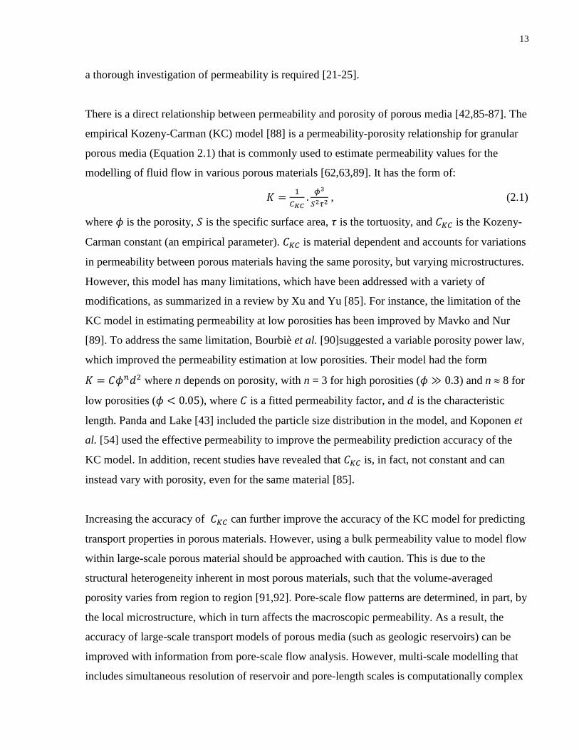
From the permeability study, it was found that the predictability of the Kozeny-Carman equation
(a commonly-used permeability relationship) can be improved with a modified KC parameter
that is an algebraic function of porosity. From the numerical stochastic tortuosity study, it was
found that tortuosity exhibits an inverse relationship with the porosity that can be expressed in
logarithmic form. Furthermore, the adjusting parameters (𝑎 and 𝑏) were calculated in the
tortuosity-porosity correlation of 𝜏 = 𝑎 − 𝑏. ln(𝜙). It was found that tortuosity increases with
increasing grain aspect ratio. From the analytical tortuosity study, it was found that the analytical
tortuosity-porosity relationships in the studied fractal geometries are linear and the tortuosity has
an upper bound at the limiting porosity (𝜙 = 0 for the Sierpinski carpet). These tools and
observations provide the capability for predicting continuous permeability and tortuosity
correlations that can be used in large-scale continuum modelling of fluid flow in porous media.

iv
Acknowledgement
I would like to sincerely thank those who have contributed to this project: Firstly, Professor
Aimy Bazylak, my supervisor, who has provided me with outstanding resources and guidance to
do this work. Secondly, I would like to extend my gratitude to my Ph.D. committee members,
Professor Markus Bussmann and David Sinton for their insightful feedback along the way. Next,
I would like to thank my lab mates for sharing their knowledge and research skills with me, and
for fostering such collaborative environment highly conducive to learning. I enjoyed all and
every moments that I spent with them in and out of lab. I was blessed that my PhD project was
partially supported by Carbon Management Canada Research Institute where I had the
opportunity to connect and collaborate with hundreds of other similar-mined investigators across
Canada. The last but not the least, I should mention that I would not be writing these words had it
not been for my caring, loving family that ensured that I was provided with every tool required to
accomplish. They have been there for me my entire life, and their unwavering support has given
me the confidence to tackle this PhD.

v
Table of Contents
Abstract ........................................................................................................................................... ii
Acknowledgement ......................................................................................................................... iv
Table of Contents ............................................................................................................................ v
List of Tables ............................................................................................................................... viii
List of Figures ................................................................................................................................ ix
1 Introduction ............................................................................................................................. 1
1.1 Background and Motivation .......................................................................................................... 1
1.2 Permeability ................................................................................................................................... 2
1.2.1 Significance of Permeability Relationships ........................................................................... 2
1.2.2 Darcy’s Law .......................................................................................................................... 3
1.2.3 Methods of Permeability Calculations .................................................................................. 4
1.3 Tortuosity ...................................................................................................................................... 6
1.4 Fractals .......................................................................................................................................... 7
1.5 Research Gap ................................................................................................................................. 8
1.6 Contributions ................................................................................................................................. 9
1.7 Organization of the Thesis ........................................................................................................... 10
2 Developing a New Form of the Kozeny-Carman Parameter for Structured Porous Media
through Lattice-Boltzmann Modelling ......................................................................................... 12
2.1 Abstract ....................................................................................................................................... 12
2.2 Introduction ................................................................................................................................. 12
2.3 Numerical Method ....................................................................................................................... 15
2.3.1 Lattice-Boltzmann Modelling .............................................................................................. 15
2.3.2 Permeability Calculations .................................................................................................... 17
2.3.3 Model Validation ................................................................................................................. 17
2.3.4 Geometry ............................................................................................................................. 18
2.3.5 Model Assumptions and Boundary Conditions ................................................................... 20
2.4 Results and Discussion ................................................................................................................ 23
2.4.1 Tortuosity Calculation ......................................................................................................... 23
2.4.2 Functional Forms ................................................................................................................. 24

vi
2.4.3 KC Parameter for Staggered Parallel Fibres ........................................................................ 25
2.4.4 Determination of KC Parameter for BCC Array of Spheres ............................................... 27
2.5 Conclusions ................................................................................................................................. 28
3 Determining the Impact of Rectangular Grain Aspect Ratio on Tortuosity-porosity
Correlations of Two-dimensional Stochastically Generated Porous Media ................................. 31
3.1 Abstract ....................................................................................................................................... 31
3.2 Introduction ................................................................................................................................. 31
3.3 Numerical Method ....................................................................................................................... 36
3.3.1 Lattice-Boltzmann Modelling .............................................................................................. 36
3.3.2 Geometry, Model Assumptions and Boundary Conditions ................................................. 37
3.3.3 Convergence Criteria ........................................................................................................... 40
3.3.4 Model Validation ................................................................................................................. 40
3.3.5 Tortuosity Calculations........................................................................................................ 41
3.3.6 Mesh-independence Study ................................................................................................... 41
3.4 Results and Discussion ................................................................................................................ 42
3.4.1 Velocity Field and Streamlines ............................................................................................ 42
3.4.2 Minimum Number of Stochastic Configurations ................................................................ 43
3.4.3 Effect of Porosity and Grain Aspect Ratio on Tortuosity .................................................... 46
3.4.4 Applicability of 2D Model .................................................................................................. 47
3.5 Conclusions ................................................................................................................................. 48
4 Analytical Tortuosity-porosity Correlations for Two Deterministic Fractal Geometries ..... 51
4.1 Abstract ....................................................................................................................................... 51
4.2 Introduction ................................................................................................................................. 51
4.3 Methodology................................................................................................................................ 56
4.3.1 Geometry ............................................................................................................................. 56
4.3.2 Analytical Model ................................................................................................................. 57
4.3.3 Sierpinski Carpet ................................................................................................................. 58
4.3.4 Circular-based Sierpinski Carpet ......................................................................................... 61
4.4 Results and Discussion ................................................................................................................ 63
4.5 Conclusions ................................................................................................................................. 68
5 Conclusions and Recommendations ...................................................................................... 71
5.1 Conclusions and Contributions .................................................................................................... 71
5.2 Future Work................................................................................................................................. 72
References ..................................................................................................................................... 74

vii
Appendix I .................................................................................................................................... 86
Appendix II ................................................................................................................................... 94
viii
List of Tables
Table 3.1 Minimum number of grains required for each porosity and grain aspect ratio
combination. .................................................................................................................................. 38
Table 3.2 Grain and domain sizes in dimensions of lattice sites. ................................................. 39
Table A-1. List of physical properties and model parameters ...................................................... 86
Table A-2. Experimental conditions used by Kueny et al. [154] .................................................. 89
Table A-3. Numerical model parameters ...................................................................................... 89

ix
List of Figures
Figure 1.1 Schematic of a carbon sequestration process and the substantial disparity among the
length scales. ................................................................................................................................... 1
Figure 1.2 Schematic of Darcy’s experiment on flow of water through sand. ............................... 5
Figure 1.3 Porous media composed of mono-sized spherical particles: (a) structured, (b)
stochastic. ........................................................................................................................................ 7
Figure 2.1 Schematic of the D2Q9 lattice employed to discretize the computational domain. .... 16
Figure 2.2 Computational domain employed for validation: (a) Schematic of quadratic fibre
distribution in the geometry used by Gebart [87]. (b) Schematic of unit cell. ............................. 17
Figure 2.3 Schematic of the staggered parallel fibre geometry: (a) Cross-section of fibres (black)
and void space (white) and (b) a unit cell (computational domain). The pixilation observed in this
figure is representative of the numerical resolution of the computational domain. ...................... 19
Figure 2.4 Schematic of a BCC unit cell employed for 3D simulations. ...................................... 20
Figure 2.5 Velocity field distribution between parallel fibres in 2D. ........................................... 22
Figure 2.6 Non-dimensionalized permeability as a function of porosity: comparing single-phase
LBM to Gebart's analytical relationship [87]................................................................................ 22
Figure 2.7 Dimensionless permeability values obtained from LB simulations, compared to values
estimated from the KC model for the parallel-cylinder structure (Figure 2.3(b)), using two forms
of 𝐶𝐾𝐶: constant 𝐶𝐾𝐶 (dotted line) and a functional form of 𝐶𝐾𝐶 (solid line). .............................. 26
Figure 2.8 Dimensionless permeability values obtained from LB simulations, compared to
estimated values from the KC model for the BCC geometry (shown in Figure 2.4). Three
alternate forms of 𝐶𝐾𝐶 were used: constant 𝐶𝐾𝐶 (dotted line), linear function of porosity (dashed
line), and third-order polynomial form (solid line) ....................................................................... 27
x
Figure 3.1 Example schematic of a (a) geometric and (b) hydraulic flow path: Note that the
hydraulic length (𝐿ℎ) is greater than the geometric length (𝐿𝑔). .................................................. 32
Figure 3.2 Possible configurations of a 2D porous medium with a porosity of 0.95, grain aspect
ratio of 1, and non-overlapping square grains. ............................................................................. 37
Figure 3.3 Example velocity distribution fields and flow streamlines within stochastically
generated 2D porous media with porosity 𝜙 = 0.85 and: (a) 𝐴𝑅 = 3, (b) 𝐴𝑅 = 1 for rectangular
grains. Tortusoities of domains (a) and (b) were calculated to be 1.23 and 1.11, respectively. ... 43
Figure 3.4 Coefficient of variation (𝐶𝑉) of tortuosity values as a function of porosity for 2D
porous media constructed with freely overlapping rectangular grains. ........................................ 44
Figure 3.5 Variation of average tortuosity with increasing number of stochastic configurations. 45
Figure 3.6 Relationship between tortuosity and porosity for 2D stochastically generated porous
media with rectangular grains of varying aspect ratio. ................................................................. 46
Figure 3.7 Relationship between the experimentally-determined adjusting parameters (𝑃)
reported by Comiti and Renaud [51] and grain aspect ratio as well as the relationship between the
numerically-determined adjusting parameters (𝑏) from the present work and grain aspect ratio.
The dashed lines connecting the data points are only intended to show the trend and do not
represent a linear fit. ..................................................................................................................... 48
Figure 4.1 Schematic of a (a) well-sorted sedimentary rock versus (b) a poorly-sorted
sedimentary rock. .......................................................................................................................... 52
Figure 4.2 Microscale (SEM) image of a granular rock sample (Pink Dolomite). ....................... 53
Figure 4.3 Construction process for the Sierpinski carpet: (a) 0th
generation, (b) 1st generation, (c)
2nd
generation; as well as for the circular-based Sierpinski carpet: (d) 0th
generation, (e) 1st
generation, (f) 2nd
generation – grey squares represent solid particles. ........................................ 54
Figure 4.4 Schematic of particle pathways through the 1st generation of the Sierpinski carpet. .. 58

xi
Figure 4.5 Schematic of particle pathways through the 1st generation of the circular-based
Sierpinski carpet. ........................................................................................................................... 61
Figure 4.6 Analytical tortuosity values of the Sierpinski carpet from present study versus
tortuosity values obtained from previous correlations [69,165] with new adjusting parameters
determined through regression analysis. ....................................................................................... 65
Figure 4.7 Analytical tortuosity values of the circular-based Sierpinski carpet from present study
versus tortuosity values obtained from previous correlations [69,165] with new adjusting
parameters determined through regression analysis. .................................................................... 66
Figure 4.8 An illustration of a highly structured porous media (where tortuosity does not
approach infinity when 𝜙 → 0)..................................................................................................... 67
Figure 4.9 The analytical tortuosity-porosity correlations for the Sierpinski carpet versus the
circular-based Sierpinski carpet. ................................................................................................... 68
Figure A-1. Developing velocity profile computed by the MRT LBM. ....................................... 87
Figure A-2. Developing velocity profile computed by the SRT LBM. ........................................ 87
Figure A-3. Centreline velocity development along the channel. ................................................ 88
Figure A-4. Schematic of the backward-facing step used in our model. ...................................... 89
Figure A-5. Velocity profile for the flow with 𝑅𝑒 = 50. ........................................................... 90
Figure A-6. Velocity profile (𝑅𝑒 = 50) from the experimental work by Kueny et al. [154]. .... 91

xii

1
1 Introduction
1.1 Background and Motivation
Characterizing the flow and transport properties in porous media is a critical component for
addressing problems in many areas of engineering and science, such as groundwater hydrology
[1], oil and gas recovery [2], carbon sequestration [3], membrane separations [4] as in fuel cells
[5], etc. These varied applications cover a vast range of length scales from the kilometer scale in
oil and gas recovery to the centimeter and millimetre scales in membrane separations or to the
micron scale for micro-fluidic devices. All these processes are, however, ultimately governed by
pore-scale phenomena, which occur at the scales of microns. Figure 1.1 illustrates a carbon
sequestration process in a saline aquifer-based reservoir and the disparity that exists between the
length scales.
Figure 1.1 Schematic of a carbon sequestration process and the substantial disparity among the length scales.
In the carbon sequestration process shown above, saline aquifers are geological porous
formations that are saturated with brine and can extend over tens of kilometers. Cap rocks are
formations with low permeabilities situated at the top of the storage zone and hinder the upward
migration of the injected CO2. Due to buoyancy forces, the injected CO2 can travel upwards up
to tens of meters before reaching the cap rock. Therefore, modelling of reservoirs such as the one

2
shown above, would involve simulations of large porous domains. It should be noted that the
fluid flow simulations in such domains are ultimately affected by the pore-scale features of the
formations.
Such a significant difference in length scales makes the simultaneous solution of macroscopic
and microscopic numerical modelling of porous media highly challenging. Therefore, at the
continuum scale (i.e. macroscopic) a porous material is typically assumed to be a homogeneous
material described by spatially averaged properties. Such spatially averaged properties are highly
dependent on the pore-scale structure of the porous formations. Therefore, a relationship
describing this dependence is required for macroscopic simulations. Such relationships can be
obtained through pore-scale investigations. Pore-scale investigations usually fall within one of
the following three categories: analytical, numerical, and experimental, each of which will be
further discussed and compared in this thesis.
A key goal of pore-scale studies is to relate a variety of structural properties (e.g. porosity) of
porous materials to flow and transport properties (e.g. permeability and tortuosity) through
macroscopic relationships. These relationships can then be used in continuum-scale modelling of
porous formations (e.g. oil reservoirs, etc).
1.2 Permeability
The permeability (𝐾) of a porous medium is a measure of its hydraulic conductivity towards
fluid flow through its pore space when subjected to an external driving force (pressure gradient).
1.2.1 Significance of Permeability Relationships
The relationship between permeability and the microstructure of a porous material is an essential
relationship, as it impacts fluid transport within the porous medium according to the Darcy’s law
[6,7] or some more advanced models [8,9]. Therefore, it can influence the efficiency of any flow
processes. Such permeability relationships are important for a wide range of applications
ranging from resin transfer moulding [10,11], biomedical engineering [12,13], recovery of oil

3
and gas and groundwater treatment [14,15], to filter separation modelling [16,17], and fuel cell
simulations [5,18].
For example, permeability relationships are critical in the oil and gas industry as an accurate
estimate of this property is needed to effectively evaluate and exploit potential resources [19].
The permeability of an oil or gas reservoir is important, for example, when determining optimal
injection rates or production rates. Permeability predictions are similarly important in carbon
sequestration as high-permeability sandstones provide desirable capacity for carbon dioxide
(CO2) storage, while low-permeability cap rocks above the storage sites are needed to confine
injected supercritical CO2 [20]. Permeability relationships are also important for studying the
subsurface flow of water. For example, for soil to be suitable for agricultural use, it must have
sufficiently high permeability to prevent waterlogging. On the other hand, it must have a
sufficiently low permeability to retain moisture and thus foster plant growth. Therefore, thorough
investigations of permeability relationships are required [21-25] for accurate modelling of the
flow transport in any of the above situations.
It should be mentioned that macroscopic approaches to fluid flow simulation in porous media use
Darcy’s law [6,7] or more complicated models [8,9]. These macroscopic (continuum-scale)
approaches require permeability as an input parameter, but permeability can vary within the
porous media. Therefore, spatially-averaged continuous permeability relationships that correlate
permeability with pore-scale properties such as porosity are needed for macroscopic flow
simulations.
1.2.2 Darcy’s Law
Permeability is one of the most common transport properties of porous materials, and it was first
introduced by Darcy in 1856 [7]. Darcy noticed that for laminar flow through saturated porous
media, the flow rate (⟨𝑢⟩) is linearly proportional to the applied pressure gradient (𝑑𝑝
𝑑𝑥). He
introduced permeability as part of the proportionality constant in Darcy’s law given below:
⟨𝑢⟩ = −𝐾
𝜇
𝑑𝑝
𝑑𝑥, (1.1)
where 𝜇 and 𝐾 are dynamic viscosity of the working fluid and the permeability of the porous

4
medium, respectively. It has been shown by numerous experimental investigations [6,8] that if
the flow rate through a porous medium is raised, pressure drop becomes no longer proportional
to fluid velocity. It is generally admitted that this deviation from Darcy’s law with increasing
fluid velocity is due to a more prominent role of inertial forces. It must be emphasized that,
although inertial forces dominate viscous forces in turbulent flow, caution must be taken not to
identify a deviation from Darcy’s law with the onset of turbulence. Turbulence occurs at 𝑅𝑒
values at least one order of magnitude higher than the 𝑅𝑒 at which deviation from Darcy’s law
occurs. In other words, the flow can be laminar but do not comply with Darcy’s law.
1.2.3 Methods of Permeability Calculations
Bulk transport properties such as permeability can be quantified by a variety of methods:
experimental, analytical, and numerical.
Most experimental methods of permeability prediction involve the application of a constant
pressure gradient across the porous medium from which the average flow velocity is determined
from the measured fluid flow-rate. The permeability of the medium is subsequently determined
using Darcy’s law [7]. Many of the earlier studies of permeability in porous media were
conducted experimentally [26-29] including the first work by Darcy in 1856 [7]. Figure 1.2
shows a schematic of Darcy’s experimental setup, which has been the basis for many
permeability-related experimental studies since.
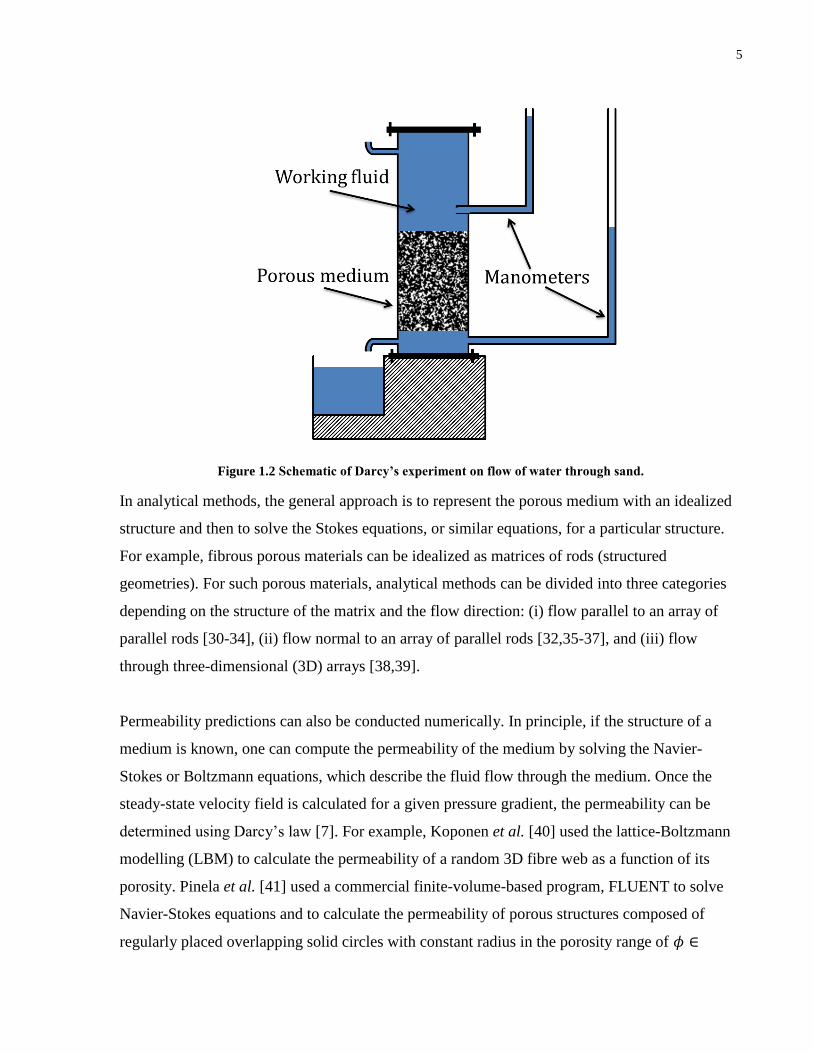
5
Figure 1.2 SchematicofDarcy’sexperimentonflowofwaterthroughsand.
In analytical methods, the general approach is to represent the porous medium with an idealized
structure and then to solve the Stokes equations, or similar equations, for a particular structure.
For example, fibrous porous materials can be idealized as matrices of rods (structured
geometries). For such porous materials, analytical methods can be divided into three categories
depending on the structure of the matrix and the flow direction: (i) flow parallel to an array of
parallel rods [30-34], (ii) flow normal to an array of parallel rods [32,35-37], and (iii) flow
through three-dimensional (3D) arrays [38,39].
Permeability predictions can also be conducted numerically. In principle, if the structure of a
medium is known, one can compute the permeability of the medium by solving the Navier-
Stokes or Boltzmann equations, which describe the fluid flow through the medium. Once the
steady-state velocity field is calculated for a given pressure gradient, the permeability can be
determined using Darcy’s law [7]. For example, Koponen et al. [40] used the lattice-Boltzmann
modelling (LBM) to calculate the permeability of a random 3D fibre web as a function of its
porosity. Pinela et al. [41] used a commercial finite-volume-based program, FLUENT to solve
Navier-Stokes equations and to calculate the permeability of porous structures composed of
regularly placed overlapping solid circles with constant radius in the porosity range of 𝜙 ∈

6
(0.22 − 0.99). A detailed description on a numerical approach (LBM) for permeability
prediction is provided in Chapter 2.
1.3 Tortuosity
Tortuosity is a measure of complexity of porous media structures and can often be realized as
elongation of streamlines (hydraulic tortuosity):
𝜏 =⟨𝐿ℎ⟩
𝐿𝑠, (1.2)
where 𝐿𝑠 is the straight-line length across the porous medium in the direction of the macroscopic
flow direction and ⟨𝐿ℎ⟩ is the average effective flow path length taken by the fluid (average
length of particle pathways). The concept of tortuosity was first introduced by Carman in 1937
[42] to match the analytical permeability results, calculated based on the primitive bundle of
capillary tubes model, to experimental data. Tortuosity is still used in (more advanced)
continuous permeability relationships to relate permeability to porosity and other pore-scale
properties of porous media such as pore connectivity, etc [43]. Tortuosity, in addition to being
used in permeability relationships, has other practical significances. For instance, in the context
of carbon sequestration, it has been found that rock formations with high tortuosities can trap
more CO2 than less tortuous formations, through a process called residual trapping [21].
Additionally, due to the increased interfacial area between CO2 and water in more tortuous
formations, dissolution rates are increased [22]. Such practical significances of tortuosity in
addition to its role in relating permeability to porosity have made tortuosity an important
parameter to be investigated.
Tortuosity can be used to characterize various aspects of porous media for example, their
hydraulic or electrical conductivity. Therefore, depending on their application and the method of
determination [44], there are several tortuosity definitions [44-49]: geometric, hydraulic,
electrical, and diffusive. These several tortuosity definitions along with their variances and
common applications will be discussed more thoroughly in Chapter 3.

7
Constitutive tortuosity models can be produced in a variety of ways: Experimental [50-52],
numerical [47,53-56] and analytical [57,58]. A more detailed discussion of tortuosity
calculations is provided in Chapters 3 and 4.
1.4 Fractals
Naturally-occurring porous media, such as sedimentary rock, rarely consist of mono-sized
particles, but rather tend to consist of large distributions of particle sizes (poorly-sorted porous
media). Nonetheless, most investigations of tortuosity in the literature (including our studies in
Chapters 2 and 3) involve porous media consisting of mono-sized (same-sized) particles, such as
the analytical studies by Yun et al. [59], Yu & Li [60], and Jian-Long et al. [61] or the numerical
studies by Koponen et al. [53,54] and Matyka et al. [47]. Figure 1.3 shows a structured and a
stochastic representation of porous media with mono-sized particles.
Figure 1.3 Porous media composed of mono-sized spherical particles: (a) structured, (b) stochastic.
One way to represent the porous media with complex and large distribution of particle sizes is to
use fractals [62-66]. Katz and Thompson [64] are among the first investigators who presented
experimental evidence indicating that the pore spaces in a set of sandstone samples conform to
fractal geometries.

8
In this thesis, fractal geometries were used to provide insight into poorly-sorted porous media,
and a novel analytical approach was presented and applied to characterize tortuosity-porosity
relationships in such geometries. A detailed review of the applied analytical approach and the
fractal geometries are presented in Chapter 4.
1.5 Research Gap
The three topics mentioned above: permeability, tortuosity, and the concept of fractals in porous
materials have proven highly useful for understanding flows in porous media; however, in
particular, there are some gaps that have not been addressed in the literature.
a) Existing continuous permeability-porosity relationships are not predictive. One such
relationship is the commonly-used semi-empirical Kozeny-Carman (KC) equation that
features a material-specific fitting parameter, 𝐶𝐾𝐶, which is generally treated as a constant
coefficient. In this work, the predictability of this relationship was improved by proposing
a modified functional form for 𝐶𝐾𝐶. Details of this contribution are discussed in Chapter 2.
b) The impact of micro-scale geometric properties of the individual grains (such as grain
aspect ratio) on the tortuosity-porosity relationships has not been extensively studied. In
this thesis, it was shown that the grain aspect ratio in 2D porous media composed of
rectangular grains impacts the adjusting parameters in the previously reported logarithmic
tortuosity-porosity correlation, 𝜏 = 𝑎 − 𝑏. ln(𝜙). Separate tortuosity-porosity relationships
were calculated for each of the three grain aspect ratios. Details related to this study are
covered in Chapter 3.
c) The Sierpinski carpet is a commonly used fractal [67-69] with a long history of application
to natural porous media [70,71] and has been frequently used for analytical studies of flow
in porous media. However, to the best of author’s knowledge, there is only one analytical
work [67] that has studied the tortuosity-porosity relationship in such structure. In this
thesis, a novel analytical approach was proposed that led to a markedly different trend for
the Sierpinski carpet tortuosity-porosity relationship presented by the previous analytical
work [67]. A tortuosity-porosity correlation for a circular-based Sierpinski carpet was also
9
obtained. The tortuosity obtained from both geometries exhibited linear relationships that
was is in agreement with the trend proposed by previous numerical [53] and experimental
works [69].
1.6 Contributions
My thesis is focused on the characterization of flow transport properties such as permeability and
tortuosity within porous media. This involved the development of a single-relaxation time (SRT)
LB model to calculate permeability. Furthermore, a multiple-relaxation time (MRT) lattice-
Boltzmann (LB) model and an analytical approach were developed to calculate tortuosity within
various porous media.
My contributions are as follows:
Improved permeability predictability of KC equation by calculating new KC parameters
for two simulated porous structures: periodic arrays of a) staggered parallel infinite
cylinders and b) spheres. The proposed KC parameters (𝐶𝐾𝐶) are functions of porosity to
ensure permeability estimation improvement for a wide range of porosity:
Published as: A. Ebrahimi Khabbazi, J. S. Ellis, A. Bazylak. Developing a new form of the
Kozeny–Carman parameter for structured porous media through lattice-Boltzmann
modeling, Computers & Fluids (2013) 75, 35 - 41
Performed a parametric study on the impact of grain aspect ratio on the tortuosity-
porosity relationships of two-dimensional (2D) porous media composed of rectangular
particles. Separate tortuosity-porosity relationships were presented for each grain aspect
ratio by calculating the adjusting parameters in the previously reported tortuosity-porosity
correlation, 𝜏=𝑎−𝑏.ln(𝜙)
Submitted as: A. Ebrahimi Khabbazi, J. Hinebaugh and A. Bazylak. Determining the impact
of rectangular grain aspect ratio on tortuosity-porosity correlations of two-dimensional
stochastically generated porous media, Physics of Fluids (Submitted in June 2015)

10
Investigated the relationships between tortuosity and porosity within two deterministic
fractal geometries by presenting and applying a novel mathematical approach on a
deterministic Sierpinski carpet and a slightly altered version of the Sierpinski carpet with
a generator that has a circular inclusion.
Published as: A. Ebrahimi Khabbazi, J. Hinebaugh and A. Bazylak. Analytical tortuosity-
porosity correlations for Sierpinski carpet fractal geometries, Chaos, Solitons and Fractals
78 (2015) 124 – 133.
My PhD research also resulted in several conference contributions [72-76].
1.7 Organization of the Thesis
This thesis is organized into five chapters. The introductory background and motivations are
presented in Chapter 1, along with an overview of the contributions of the thesis. Chapter 2 is
focused on permeability predictions through numerical modelling (SRT LBM). A detailed
description of the SRT LBM is also presented. New functional forms of KC parameter (𝐶𝐾𝐶) are
determined for the two porous structures of: periodic arrays of a) staggered parallel infinite
cylinders and b) spheres. Chapter 3 is focused on tortuosity calculations through numerical
modelling (MRT LBM). The impact of the geometric properties of the individual grains, (such as
grain aspect ratio) on the tortuosity-porosity relationships in porous media using stochastic
numerical modelling is investigated. This impact is quantified by fitting our tortuosity data to the
previously reported logarithmic tortuosity-porosity correlation, 𝜏 = 𝑎 − 𝑏. ln(𝜙) and calculating
new adjusting parameters. As a result, spatially-averaged continuous tortuosity-porosity
relationships are provided for 2D stochastically generated porous media composed of rectangular
grains with distinct aspect ratios. The minimum number of required stochastic simulations is
determined in each case. Chapter 4 is focused on analytical calculation of tortuosity in two
deterministic fractals (a Sierpinski carpet and a circular-based Sierpinski carpet). A novel
mathematical approach for calculating tortuosity is presented in this chapter. Conclusions and a
road map for future work are provided in Chapter 5.

11

12
2 Developing a New Form of the Kozeny-Carman
Parameter for Structured Porous Media through
Lattice-Boltzmann Modelling1
2.1 Abstract
The semi-empirical Kozeny-Carman (KC) equation is a commonly-used relationship for
determining permeability as a function of porosity for granular porous materials. This model
features a material-specific fitting parameter, 𝐶𝐾𝐶, which is generally treated as a constant
coefficient. Recent studies, however, have shown that 𝐶𝐾𝐶 is not constant and could be a varying
function of porosity. LBM was used to calculate the absolute permeability of two simulated
porous structures: periodic arrays of a) staggered parallel infinite cylinders and b) spheres.
Various functional forms of 𝐶𝐾𝐶 was then identified and for each form, a regression analysis was
performed in order to fit the function to the permeability values determined from the LB
simulations. From this analysis, optimal fitting parameters were extracted for each function that
minimized the error between permeability values obtained from the KC model and the LB
simulations. All linear and non-linear functional forms proposed in this work improve the
predictability of the KC model. An algebraic function for 𝐶𝐾𝐶 provided the most accurate
prediction of the KC porosity-permeability relationship for the geometries examined.
2.2 Introduction
The study of flow in porous media is of crucial importance in many fields, including geophysics
and soil science [3,77-81]. An important area still under investigation is the relationship between
the porous microstructure and the permeability of a material [82-84]. This is an essential
relationship, as it impacts fluid transport within the porous medium and can influence the
efficiency of any flow process. For example, in carbon sequestration, high-permeability
sandstones provide desirable capacity for carbon dioxide (CO2) storage, while low-permeability
cap rocks above the storage sites are needed to confine injected supercritical CO2 [20]; therefore
1 This chapter is based on a published work: Ebrahimi Khabbazi A, Ellis JS, Bazylak A. Developing a new form of
the Kozeny-Carman parameter for structured porous media through lattice-Boltzmann modeling. Comput. Fluids
2013;75:35-41.
13
a thorough investigation of permeability is required [21-25].
There is a direct relationship between permeability and porosity of porous media [42,85-87]. The
empirical Kozeny-Carman (KC) model [88] is a permeability-porosity relationship for granular
porous media (Equation 2.1) that is commonly used to estimate permeability values for the
modelling of fluid flow in various porous materials [62,63,89]. It has the form of:
𝐾 =1
𝐶𝐾𝐶.𝜙3
𝑆2𝜏2, (2.1)
where 𝜙 is the porosity, 𝑆 is the specific surface area, 𝜏 is the tortuosity, and 𝐶𝐾𝐶 is the Kozeny-
Carman constant (an empirical parameter). 𝐶𝐾𝐶 is material dependent and accounts for variations
in permeability between porous materials having the same porosity, but varying microstructures.
However, this model has many limitations, which have been addressed with a variety of
modifications, as summarized in a review by Xu and Yu [85]. For instance, the limitation of the
KC model in estimating permeability at low porosities has been improved by Mavko and Nur
[89]. To address the same limitation, Bourbiè et al. [90]suggested a variable porosity power law,
which improved the permeability estimation at low porosities. Their model had the form
𝐾 = 𝐶𝜙𝑛𝑑2 where n depends on porosity, with n = 3 for high porosities (𝜙 ≫ 0.3) and n 8 for
low porosities (𝜙 < 0.05), where 𝐶 is a fitted permeability factor, and 𝑑 is the characteristic
length. Panda and Lake [43] included the particle size distribution in the model, and Koponen et
al. [54] used the effective permeability to improve the permeability prediction accuracy of the
KC model. In addition, recent studies have revealed that 𝐶𝐾𝐶 is, in fact, not constant and can
instead vary with porosity, even for the same material [85].
Increasing the accuracy of 𝐶𝐾𝐶 can further improve the accuracy of the KC model for predicting
transport properties in porous materials. However, using a bulk permeability value to model flow
within large-scale porous material should be approached with caution. This is due to the
structural heterogeneity inherent in most porous materials, such that the volume-averaged
porosity varies from region to region [91,92]. Pore-scale flow patterns are determined, in part, by
the local microstructure, which in turn affects the macroscopic permeability. As a result, the
accuracy of large-scale transport models of porous media (such as geologic reservoirs) can be
improved with information from pore-scale flow analysis. However, multi-scale modelling that
includes simultaneous resolution of reservoir and pore-length scales is computationally complex

14
and expensive. Experimental determination of local permeability values can be expensive and
time-consuming, and assigning an accurate universal permeability function to a particular class
of porous materials remains a challenge. An alternative approach is to numerically simulate fluid
transport at the microscale and use the results to inform appropriately partitioned simulations at
the reservoir-scale.
A variety of numerical schemes are available for simulating flow in porous media at short length
scales [93-96]. These include pore-network modelling (PNM), Navier-Stokes (NS) based
computational fluid dynamics (CFD) techniques, and LBM. PNMs have attractive features
(computational efficiency and capability of handling large domain sizes), but it is difficult to
produce a topologically-equivalent network for certain classes of rocks with this method [25].
Another drawback of PNM includes the inability to resolve the velocity and concentration
gradients within a single pore. CFD and LBM both can be employed to resolve the in-pore
gradients; however, they differ from each other in various aspects. Some major differences are as
follows:
NS equations are second-order partial differential equations (PDEs); however, Boltzmann
equation (LBE) is derived from a first order PDE, i.e. the Boltzmann equation.
The convection operator of the NS equations is a nonlinear term, where all the terms of
the LBE are linear due to the lattice Bhatnagar–Gross–Krook (BGK) simple collision
operator.
In the LBM, pressure is calculated using an algebraic equation of state, while CFD
solvers for the incompressible NS equations need to solve the Poisson equation for the
pressure, which is an elliptic second order PDE and involves global data communication.
In contrast, data communication in LBM is always local which, which makes the LBM
highly parallelizable. Only adjacent lattice nodes are considered for the computation of
local distribution functions [97,98].
Significant advancements have been made through the application of LBM in the study of
transport in porous media, specifically in areas such as single-phase flow in reconstructed porous
domains [99], modelling of evaporation [100], binary fluid flows [101], heat transfer [102,103]
and multiphase flows [104-107].
15
In this investigation, a novel methodology for rapidly and accurately evaluating various forms of
the KC equation and its parameter, 𝐶𝐾𝐶, is presented and demonstrated through LBM of fluid
flow within two geometries: i) a staggered array of infinite parallel cylinders and ii) a periodic
array of spheres. The work presented here provides a valuable method for obtaining
permeability-porosity relationships needed for informing coupled mass and momentum
equations, such as the Brinkman equation solution in reservoir-scale modelling [108].
2.3 Numerical Method
2.3.1 Lattice-Boltzmann Modelling
In this study, a single-relaxation time (SRT) LBM was employed to simulate single phase flow in
porous geometries, which includes a 2D representation of a staggered array of parallel fibres and
a 3D representation of a body-centred cubic (BCC) array of spheres. These geometries have been
broadly studied in the literature [36,37,87], providing opportunities for validation for this
methodology. The approach presented here can be applied to representative elementary volumes
at the pore scale to inform reservoir scale modelling. The SRT LBM consists of a discretized
Boltzmann equation to approximate the compressible NS equations in the nearly-incompressible
limit [109]. For the discretization to be accurate, a low Mach number condition must be satisfied
[110,111], as is the case here (𝑀𝑎 ≈ 10-5
).
The LB method involves an iterative sequence of propagations and collisions of fictitious
particles at the lattice nodes of a discretized domain. The mass density of each non-solid node is
defined by a set of scalar particle distribution functions (PDF; f in Equation 2.2, below), each of
which is related to a lattice velocity unit vector. At each time step, the PDFs are shifted to
neighboring nodes according to their unit velocity vector through the propagation process (also
known as streaming). Following each streaming step, a collision step is performed, whereby the
value of each PDF is updated by applying an algebraic collision operator. In its simplest form,
the collision operator is based on the BGK approximation [112].
Streaming and collision of the fictitious particles are encapsulated in the LB equation, as shown

16
in Equation 2.2 [113]:
𝑓𝑖(�� + 𝑐𝑖𝑒𝑖 ∆𝑡, 𝑡 + ∆𝑡) − 𝑓𝑖(��, 𝑡) = −1
𝜏𝑅[𝑓𝑖(��, 𝑡) − 𝑓𝑖
𝑒𝑞(��, 𝑡)], (2.2)
where 𝑐𝑖 =∆𝑥
∆𝑡 is the magnitudes of discrete lattice velocities, ∆𝑥 is the lattice spacing, and ∆𝑡
represents the time step in lattice units (equal to unity here). 𝜏𝑅 is the dimensionless relaxation
time, 𝑒𝑖 are the velocity basis vectors, and 𝑓𝑖 is the probability distribution function. 𝑓𝑖𝑒𝑞
is the
corresponding equilibrium distribution function, given by Equation 2.3 [114]:
𝑓𝑖𝑒𝑞 = 𝜌𝑤𝑖 [1 +
3
𝑐2𝑒𝑖 �� +
9
2𝑐4(𝑒𝑖 ��)
2 −3
2𝑐2��. ��], (2.3)
where �� denotes the velocity field, 𝜌 represents the density in lattice units, and 𝑤𝑖 are the weight
coefficients. The corresponding equilibrium distribution is a low Mach-number truncated
Maxwell-Boltzmann distribution [115] In Equation 2.2, the left-hand side represents the
streaming step, wherein the PDFs are shifted based on their velocities, and the right-hand side
describes the collision operator. In this study, the D2Q9 model (two dimensions with nine
directional velocities; Figure 2.1) was used for 2D simulations and D3Q19 for 3D modelling
[114]. For the D2Q9 lattice, 𝑤𝑖 =1
9,4
9𝑎𝑛𝑑
1
36, whereas for D3Q19, 𝑤𝑖 =
1
3,1
18𝑎𝑛𝑑
1
36 in
Equation 2.3.
Figure 2.1 Schematic of the D2Q9 lattice employed to discretize the computational domain.
Macroscopic quantities such as density, velocity, and pressure can be determined from the
distribution function 𝑓𝑖(��, 𝑡) [98]:
𝜌 = ∑ 𝑓𝑖𝑖 , (2.4-a)
𝜌�� = ∑ 𝑒𝑖𝑓𝑖𝑖 , (2.4-b)
𝑃 = 𝜌𝑐𝑠2, (2.4-c)
where 𝑐𝑠 denotes the speed of sound in lattice units (equal to 1/√3), and 𝑃 denotes the pressure.
1
2
3
4
56
78
0

17
The kinematic viscosity 𝜈 is given by:
𝜈 =𝛿𝑥2
𝛿𝑡𝜈𝑙, (2.5)
where 𝜈𝑙 is the kinematic viscosity in lattice units, 𝜈𝑙 = (𝜏𝑅 − 0.5)𝑐𝑠2 [98].
2.3.2 Permeability Calculations
The numerical model of fluid flow within a porous material can be used in combination with
Darcy’s law (Equation 2.6) to calculate permeability of the porous medium of interest.
⟨𝑢⟩ = −𝐾
𝜇. ∇𝑃, (2.6)
where ⟨𝑢⟩ denotes the volume-averaged flow velocity, K is the permeability of the porous
medium under investigation, 𝜇 is the dynamic viscosity of the fluid, and ∇𝑃 represents the
pressure gradient vector. To avoid inaccuracies due to eddies, Darcy’s law is only accurate in the
limit of viscous (or creeping) flow (pore-scale Reynolds numbers (𝑅𝑒) < 1) [116]. 𝑅𝑒 < 0.1
for all the simulations presented here. All computations were performed in MATLAB (R2010b).
2.3.3 Model Validation
To determine appropriate grid spacing, a mesh-refinement study was performed on the 2D
fibrous geometry. The ideal lattice spacing was determined to be 144 lattices nodes in each
direction (length and width) for the range of fibre radii studied (30-165 µm). The numerical
model was then validated with Gebart’s analytical solution for permeability of a quadratic
(square) fibre arrangement (Figure 2.2), assuming parabolic flow.
Figure 2.2 Computational domain employed for validation: (a) Schematic of quadratic fibre distribution in
the geometry used by Gebart [87]. (b) Schematic of unit cell.
Direction
of flow
Direction
of flow
(a) (b)

18
Gebart performed a combined theoretical, numerical, and experimental study of the permeability
of ordered arrays of fibres and presented the following permeability-porosity relationship in the
limit of closed-packed fibres [87,117]:
𝐾
𝑅2= 𝐶𝐺 (√
1−𝜙𝑐
1−𝜙− 1)
5
2
, (2.7)
where 𝑅 is the fibre radius (𝐾
𝑅2 is the non-dimensionalized permeability), 𝜙 is the porosity, and
𝜙𝑐 is the critical porosity below which flow does not occur (i.e. percolation threshold). 𝐶𝐺 is a
proportionality constant, also known as the geometric factor, which Gerbart calculated to be
𝐶𝐺 =16
9𝜋√2 for the quadratic fibre arrangement. Gebart showed that the analytically-determined
permeability was in agreement with a finite difference solution of the NS equations, for porosity
values up to 0.65. To facilitate our numerical validation, the geometric factor and critical
porosity employed by Gebart was used: 𝐶𝐺 =16
9𝜋√2 and 𝜙𝑐 = 1 −
𝜋
4 [87].
2.3.4 Geometry
Transport phenomena in some structures can be efficiently modelled in 2D with significant
computational savings and without compromising accuracy. Perpendicular flow over arrays of
infinite parallel fibres is an example of a 2D simulation that is representative of the 3D case.
There are, however, situations where 3D modelling is required, such as when the geometry and
flow fields are not symmetric. In this study, two separate geometries were investigated: a) a
staggered array of parallel fibres (2D), and b) a 3D BCC array of spheres, which cannot be
accurately modelled in 2D.
The staggered array of parallel fibres were represented by a 2D domain consisting of staggered
arrays of identical disks with radius,𝑅, (Figure 2.3(a)). The fibres are arranged in a periodic
pattern so that only a single unit cell with periodic boundary conditions is required (Figure
2.3(b)).

19
Figure 2.3 Schematic of the staggered parallel fibre geometry: (a) Cross-section of fibres (black) and void
space (white) and (b) a unit cell (computational domain). The pixilation observed in this figure is
representative of the numerical resolution of the computational domain.
The size of the computational domain was chosen to be 480 µm in both length and width. The
centre-to-centre distance between two adjacent solid circles was constant over the domain and set
to 340 µm. This was the same characteristic length employed by Kang et al. [118] in their pore-
scale study of reactive transport involved in geologic CO2 sequestration. The same characteristic
length has also been employed here in order to facilitate future comparison with the above-
mentioned study. Porosities were varied by changing the radius of the fibres. To remain
consistent with the 2D structure, the size of the 3D domain (Figure 2.4) was also set to
480µm480µm480µm.
Solid
Void
2R
480 µm
x
y
(a) (b)
Direction of flow

20
Figure 2.4 Schematic of a BCC unit cell employed for 3D simulations.
2.3.5 Model Assumptions and Boundary Conditions
The underlying motivation for this work is to determine the permeability of deep saline aquifers
for CO2 sequestration, where CO2 is injected into geological porous formations. One method of
CO2 sequestration entitled “surface dissolution” involves the CO2 saturation of extracted brine,
followed by the injection of the saturated solution into geological formations. In this work, a
CO2-saturated brine solution at 65oC with a salinity of 85000 ppm (NaCl) was modelled [119].
Despite this assumption, the results presented are general, since the Reynolds number is
sufficiently low (𝑅𝑒 ≪ 1). In these conditions, permeability is found to be independent of the
fluid properties such as, viscosity, density and pressure gradient [116]. A density of 1.041 g/cm3
and a dynamic viscosity of 0.6025 cP were employed. To generate creeping flow, a constant
pressure gradient boundary condition of 0.19 Pa was imposed between the inlet and outlet.
Periodic and bounce-back boundary conditions were employed at the side boundaries and the
surface of the solid materials, respectively. The bounce-back scheme, equivalent to the no-slip
boundary condition, was implemented via the direct reflection of fictitious particles impacting a
solid boundary [120].
Care must be exercised when using SRT LBM, as the permeability of the porous medium could

21
become unrealistically dependent on the kinematic viscosity, ν [121]. Since the kinematic
viscosity is a function of the relaxation time, 𝜏𝑅 , (Equation 2.5), an informed choice of 𝜏𝑅 is
essential. By selecting a suitable 𝜏𝑅value, the 𝜏𝑅 dependence in SRT LBM simulations can be
alleviated. Note that a 𝜏𝑅 value that is too low can lead to non-physical system properties,
whereas if it is too high, the system will not converge. Pan et al. [93] reported that the results
obtained using SRT LBM are less dependent on the relaxation time for 𝜏𝑅 near unity. Therefore,
in this study, the relaxation time was set to 1. It should be noted that a multiple-relaxation time
approach (MRT) may be employed to mitigate this problem [122]. This method is more robust
than the SRT method, but comes at the cost of increased complexity.
To ensure that the simulation of a single unit cell is an appropriate choice for the computational
domain, various domain sizes were examined. It was found that the permeability calculated from
a single unit cell with periodic boundary conditions is identical to that calculated for larger
domains consisting of up to five unit cells, in both the horizontal and vertical directions. Based
on this result, simulations were carried out on a single unit cell throughout this study.
Figure 2.5 shows the LBM-derived velocity field distribution within the porous media with a
staggered array of infinite parallel cylinders previously employed by Gebart [87]. The velocity
distribution calculated here demonstrates the ability of LBM to resolve gradients at the pore-
scale, and as expected this distribution is parabolic.

22
Figure 2.5 Velocity field distribution between parallel fibres in 2D.
To compare our permeability results from LBM to those from Gebart’s analytical solution, the
dimensionless permeability was defined as follows:
𝐾𝑁𝐷 =𝐾
𝑅2, (2.8)
where 𝐾𝑁𝐷is the non-dimensionalized permeability. Figure 2.6 illustrates the close agreement
between the permeability-porosity relationship determined from the LB simulations and Gebart’s
analytical solution.
Figure 2.6 Non-dimensionalized permeability as a function of porosity: comparing single-phase LBM to
Gebart's analytical relationship [87].

23
2.4 Results and Discussion
In the following section, the results of the LB simulations for the two examined geometries are
presented. First, the model used to compute the tortuosity, which is then used to determine the
permeability from the KC equation (Equation 2.1) is discussed. It is important to note that the
final fitting parameters in the permeability relationships will depend on the definition of
tortuosity used. Next, the functional forms of 𝐶𝐾𝐶 that will be used to modify the KC equation
are presented. Finally, the permeabilities obtained from the simulations to modify the KC
relationship (Equation 2.1) by determining functional expressions for the 𝐶𝐾𝐶 parameter are
compared.
2.4.1 Tortuosity Calculation
In this study, tortuosity, 𝜏, is computed as the ratio of the average of the actual path lengths (as
determined from the LB simulations) to the length of the system in the direction of the
macroscopic flux [53]. This is given by Equation 2.9 [56]:
𝜏 =∑ 𝑈𝑚𝑎𝑔(𝑖,𝑗)𝑖,𝑗
∑ |𝑈𝑥(𝑖,𝑗)|𝑖,𝑗, (2.9)
where, 𝑈𝑥 is the 𝑥-direction velocity component, and 𝑈𝑚𝑎𝑔 is the velocity magnitude:
𝑈𝑚𝑎𝑔(𝑖, 𝑗) = √𝑈𝑥(𝑖, 𝑗)2 + 𝑈𝑦(𝑖, 𝑗)2, (2.10)
for all lattice nodes 𝑖, 𝑗 in the system. This method was chosen as it accounts for both the
microscopic flow and the geometry in the tortuosity calculation [53,56]. However, the main
advantage of this method is that it does not require streamline calculations, which is a
sophisticated, time-consuming and error-prone task, especially in realistic 3D geometries.
Instead, it allows for calculation of the streamline tortuosity directly from the velocity field.
Therefore, one can compute the tortuosity of practically any fluid flow system in which the
velocity field is determined, whether numerically, analytically or experimentally.
It is important to note that the final expression for 𝐶𝐾𝐶 will depend on the definition of tortuosity
used. Other methods have been used to compute tortuosity [48,53,56]. One such description is
the ratio of the shortest continuous path between any two points in the pore space to the distance

24
between the same two points on a straight line in the direction of the mean flow [53]; however,
this method only considers the geometry, and does not account for the complexity of the flow or
transport mechanisms.
2.4.2 Functional Forms
To improve the accuracy of the KC equation in predicting the porosity-permeability relationship
for flow in porous media, alternate forms of the KC parameter were considered. Davies and
Dollimore [123] and Kyan et al. [124] found that 𝐶𝐾𝐶 first decreases with porosity, at low
porosities, then increasing at higher values. Davies and Dollimore [123] suggested a rational
form for 𝐶𝐾𝐶 for sedimenting sphere beds and found that the specific geometry under
consideration would determine the order of the rational function. Kyan et al. [124] proposed a
more detailed rational function for fibrous materials, which incorporated the viscous friction
factor. For their specific porous geometries, they found a minimum in 𝐶𝐾𝐶 near 𝜙 = 0.85. Happel
and Brenner [125] reported experiments on a variety of structured materials and showed that 𝐶𝐾𝐶
may be a monotonically increasing function of porosity. All of the behaviors described above can
be modelled using exponential, power-law, logarithmic or algebraic functions.
To improve the predictability of the KC equation for describing the porosity-permeability
relationship for flow in porous media, five alternative functional forms for the 𝐶𝐾𝐶 parameter
(used in Equation 2.1) were examined. In addition to the conventionally-used constant 𝐶𝐾𝐶
(Equation 2.11-a), the five functional forms are listed below (Equations 2.11-b−2.11-f):
𝐶𝐾𝐶 = 𝐴, (2.11-a)
𝐶𝐾𝐶 = 𝐴𝜙 + 𝐵, (2.11-b)
𝐶𝐾𝐶 = 𝐴𝑎𝐵𝜙, (2.11-c)
𝐶𝐾𝐶 = 𝐴 log𝐵 𝜙 + 𝐶, (2.11-d)
𝐶𝐾𝐶 = 𝐴(𝜙 − 𝐶)𝐵, 𝐵 ∈ 𝑁, (2.11-e)
𝐶𝐾𝐶 = 𝐴|𝜙 − 𝐶|𝐵 + 𝐷,𝐵 ∈ 𝑅, (2.11-f)
where 𝐴, 𝐶, and 𝐷 are real fitting parameters, and 𝐵 is either natural (Equation 2.11-e) or real
(Equation 2.11-f). The permeability-porosity relationship determined for each functional form is
compared to that determined from the LB simulations. These are all compared with the results

25
using the constant KC parameter (Equation 2.11-a).
Each functional form was evaluated by comparing it to the LB results using a nonlinear
regression analysis employing the Generalized Reduced Gradient (GRG2) algorithm [126]. To
this end, the permeability and tortuosity values obtained from the LB simulations were used to
determine optimal fitting parameters for the 𝐶𝐾𝐶 functions that minimize the error in
permeability between the simulated values and those calculated from Equation 2.1. The error
function used in the regression analysis to determine the algebraic fitting parameters was the
sum-squared difference between log-values of the computed and simulated permeabilities. The
GRG2 algorithm was implemented using the Microsoft Excel Solver (Microsoft Excel, version
14.0).
2.4.3 KC Parameter for Staggered Parallel Fibres
The LB model was applied to a 2D porous structure consisting of a staggered array of identical
disks (representing infinite parallel fibres in 3D) to find a suitable expression for 𝐶𝐾𝐶. In the KC
equation, specific surface area, S, is calculated as the solid phase surface area per unit volume of
the unit cell.
The non-dimensionalized permeability obtained from the LB simulations is compared to those
calculated from the KC equation (Equation 2.1) with two forms of 𝐶𝐾𝐶 in Figure 2.7. The
calculated non-dimensionalized permeability values were determined using two forms of the KC
parameter. First, 𝐶𝐾𝐶 was assumed constant, as in the original KC model [127]. The best-fit value
for this was found to be 2.409. However, this form of the KC parameter failed to reproduce
accurate permeability values for the entire porosity range considered.

26
Figure 2.7 Dimensionless permeability values obtained from LB simulations, compared to values estimated
from the KC model for the parallel-cylinder structure (Figure 2.3(b)), using two forms of 𝑪𝑲𝑪: constant 𝑪𝑲𝑪
(dotted line) and a functional form of 𝑪𝑲𝑪 (solid line).
The KC value used in the original model was 𝐶𝐾𝐶 = 2, which is comparable to the fitted value of
2.409. This discrepancy in 𝐶𝐾𝐶 can be attributed to variations between the geometries used. In
the original model [87], the porous medium was formed of 𝑁 identical parallel tubes through a
solid block, whereas in our model, the flow is around solid parallel fibres. The model with
constant 𝐶𝐾𝐶 does not provide accurate results. For instance, there is an error of 40% in the
permeability prediction at a porosity of 0.42, as can be seen from the deviation between the
dotted line and LBM data points in Figure 2.7.
A non-linear algebraic function of porosity was found to provide an appropriate relationship
(Equation 2.11-f), where, A, 𝐵, 𝐶 and 𝐷 were determined to be 5420, 5.6, 0.6 and 3.38
respectively. This functional form for 𝐶𝐾𝐶 was derived for an approximate porosity range of
𝜙 ∈ (0.25 − 0.97). Figure 2.7 demonstrates an improved fit of the model using the algebraic
form in Equation 2.11-f (solid line), as opposed to the constant-value 𝐶𝐾𝐶 (dotted line). The
functional form reduces the error from 40% to 8% in permeability prediction at a porosity of
0.42. The fitted values obtained for A, 𝐵, 𝐶 and 𝐷 in Equation 2.11-f depend on the method used
to calculate the tortuosity.

27
2.4.4 Determination of KC Parameter for BCC Array of Spheres
For the study involving a 3D domain, a staggered array of spheres was employed, which is
similar to the packed-bed-of-beads geometry used in an early extension of the original KC
equation [42]. In that study, a value of 𝐶𝐾𝐶 = 5 was used. Due to the similarity between the
geometries, it was expected a similar value for 𝐶𝐾𝐶 for our BCC structure. The best fit-value for
𝐶𝐾𝐶 found for the LB simulations was 5.63, using a constant 𝐶𝐾𝐶 value. Figure 2.8 shows the
dimensionless permeability values obtained from the numerical simulations and from the KC
equation for the BCC unit cell. As can be seen from the dotted line, a constant 𝐶𝐾𝐶 value is not
an appropriate choice, as the discrepancy between the LBM results and the KC model reaches
26% at a porosity of 0.42.
Figure 2.8 Dimensionless permeability values obtained from LB simulations, compared to estimated values
from the KC model for the BCC geometry (shown in Figure 2.4). Three alternate forms of 𝑪𝑲𝑪 were used:
constant 𝑪𝑲𝑪 (dotted line), linear function of porosity (dashed line), and third-order polynomial form (solid
line)
As shown above, the KC model with constant 𝐶𝐾𝐶 for the BCC structure was more accurate than
for the infinite parallel cylinder geometry discussed above. The predictability of the KC model
for the BCC case was further improved by using a linear expression (Equation 2.11-b) for 𝐶𝐾𝐶.
This improvement is shown in Figure 2.8 (dashed line). For example, the discrepancy in the
permeability prediction of the KC model at 0.42 porosity decreased to 4% when a linear function
of porosity (Equation 2.11-b) was employed for 𝐶𝐾𝐶. The linear form of the KC parameter

28
(Equation 2.11-b) utilized to improve the predictability of the KC model. The fitting coefficients
A and B were found to be 9.63 and 0.02, respectively. This functional form for 𝐶𝐾𝐶 was derived
for an approximate porosity range of 𝜙 ∈ (0.34 − 0.83).
Permeability estimations by the KC model were further enhanced by adopting a higher-order
polynomial, though the improvement was only moderate. The linear form of 𝐶𝐾𝐶 provides
sufficient accuracy, without increasing the complexity or error introduced with more variables.
This was not the case for the staggered array of parallel cylinder geometry, as various types of
functions were examined in an effort to reproduce the pore-scale numerical results. The reason
for the complexity in the parallel cylinder 𝐶𝐾𝐶 expression was the significant variation of
permeability values with porosity. This large variation is mainly due to the arrangement of solid
space in parallel-cylinder structure, as opposed to the BCC geometry. For instance, in the BCC
geometry, there is a pathway for fluid particles even if the spheres are in contact, while this is not
the case for the infinite parallel-cylinder geometry. To capture permeability values for a wide
range of porosity, a highly-nonlinear function of porosity was required for the parallel-cylinder
geometry, as opposed to a simple linear expression for the BCC case (Equation 2.11-b).
In this work, further evidence that the 𝐶𝐾𝐶 parameter is not constant has been provided, and
instead is a function of porosity, as previous studies have suggested [85,128]. An efficient
numerical approach that can be used to rapidly evaluate various forms of the KC relationship has
been validated and applied. This numerical approach will be a useful tool for researchers, as
experimental approaches for determining permeability are often expensive and time-consuming
compared to numerical schemes [25]. The LB model used for this investigation presents a rapid
method of determining an appropriate 𝐶𝐾𝐶 for porous materials
2.5 Conclusions
To determine the proper form of the KC parameter for a specific material, many permeability
measurements must be performed over a large range of porosities. Since such experiments are
often costly and time-consuming, a numerical approach was developed to characterize alternate
forms of the KC equation. In this study, an SRT LB model of single-phase flow within porous
media was presented and validated with an analytical permeability-porosity relationship [87].

29
Both the staggered array of infinite parallel cylinders and the body-centred cubic (BCC) array of
spheres required a functional form for the KC parameter to be accurately determined over the
range of porosities considered. The LB model developed for this investigation is a valuable tool
for calculating the 𝐶𝐾𝐶 parameter for a variety of porous media. For the application of carbon
sequestration, which may involve heterogeneously structured geologic formations, the
methodology presented here can be employed to determine the permeability-porosity relationship
for various locally-homogeneous regions throughout the reservoir. In future studies, micro-CT
images of the porous medium of interest can be incorporated into the LB simulations.

30

31
3 Determining the Impact of Rectangular Grain
Aspect Ratio on Tortuosity-porosity Correlations
of Two-dimensional Stochastically Generated
Porous Media2
3.1 Abstract
Stochastic numerical modelling is a powerful tool for estimating bulk transport properties of
porous media, such as tortuosity. However, stochastic numerical modelling has not been used
extensively to investigate the impact of the geometric properties of the individual grains, (such as
grain aspect ratio) on the tortuosity-porosity relationships in porous media. The impact of grain
aspect ratio on the tortuosity-porosity relationships of 2D porous media composed of rectangular
particles was determined by calculating the adjusting parameters in the previously reported
logarithmic tortuosity-porosity correlation, 𝜏 = 𝑎 − 𝑏. ln(𝜙). These adjusting parameters were
then obtained by calculating average tortuosity values with grain aspect ratios of ∈ {1, 2, 3} and a
porosity range of ∈ [0.55 − 0.95]. A minimum of 6, 8 and 10 stochastic simulations were also
determined for grain aspect ratios of ∈ {1, 2, 3}, respectively, to be required to calculate these
average tortuosity values in laminar flow (𝑅𝑒 ≪ 1). The minimum number of required stochastic
simulations is highly valuable for the efficient numerical determination of tortuosity-porosity
relationships.
3.2 Introduction
Permeability and effective diffusivity are valuable material properties for predictive continuum
models of flow and mass transport through porous media. When empirical values for these
properties are not available, estimates can be made based on porosity and tortuosity values.
Tortuosity, 𝜏, provides a means of measuring the complexity of fluid pathways through a porous
material and has been strongly correlated to material porosity [54,129]. Therefore, tortuosity has
been applied in numerical models for science and engineering applications ranging from oil
2 This chapter is based on a submitted paper: Ebrahimi Khabbazi A, Hinebaugh J, and Bazylak A. Determining the
impact of rectangular grain aspect ratio on tortuosity-porosity correlations of two-dimensional stochastically
generated porous media, Physics of Fluids (Submitted in June 2015)

32
recovery and carbon sequestration to fuel cells [118,130-133].
There are several definitions of tortuosity in the literature [44-49], depending on characterization
needs, ranging from the determination of electrical conductivity to hydraulic conductivity.
Several tortuosity definitions along with their variances and common applications are discussed
below to emphasize the importance of implementing tortuosity definitions with care.
The geometrical tortuosity, 𝜏𝑔, can be defined as the ratio of the average length of the geometric
flow paths, ⟨𝐿𝑔⟩, to the length of the medium in the direction of macroscopic flux, 𝐿𝑠, [44]:
𝜏𝑔 =⟨𝐿𝑔⟩
𝐿𝑠, (3.1)
while the hydraulic tortuosity, 𝜏, is defined as the ratio of the average effective flow path length
taken by the fluid, ⟨𝐿ℎ⟩, to the straight-line length across the medium, 𝐿𝑠 [55]:
𝜏 =⟨𝐿ℎ⟩
𝐿𝑠. (3.2)
Geometric pathways include the shortest paths consisting of straight lines touching and passing
by grains with close tangents (Figure 3.1(a)), whereas in reality, fluid particles are expected to
travel through smoothed streamlines [44,46]. Therefore, 𝜏 is always greater than 𝜏𝑔.
Furthermore, geometrical tortuosity is commonly based on geometric parameters, such as
particle size, shape, and arrangement.
Figure 3.1 Example schematic of a (a) geometric and (b) hydraulic flow path: Note that the hydraulic length
(𝑳𝒉) is greater than the geometric length (𝑳𝒈).
Hydraulic tortuosity accounts for the hydrodynamics of the flow within porous formations
(Figure 3.1(b)). Hydraulic tortuosity is used to determine the permeability of porous media. For
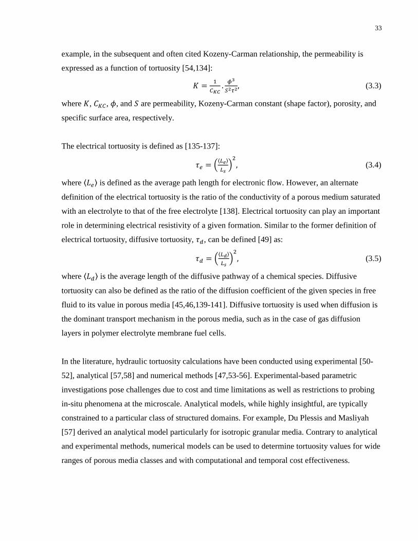
33
example, in the subsequent and often cited Kozeny-Carman relationship, the permeability is
expressed as a function of tortuosity [54,134]:
𝐾 =1
𝐶𝐾𝐶.𝜙3
𝑆2𝜏2, (3.3)
where 𝐾, 𝐶𝐾𝐶, 𝜙, and 𝑆 are permeability, Kozeny-Carman constant (shape factor), porosity, and
specific surface area, respectively.
The electrical tortuosity is defined as [135-137]:
𝜏𝑒 = (⟨𝐿𝑒⟩
𝐿𝑠)2
, (3.4)
where ⟨𝐿𝑒⟩ is defined as the average path length for electronic flow. However, an alternate
definition of the electrical tortuosity is the ratio of the conductivity of a porous medium saturated
with an electrolyte to that of the free electrolyte [138]. Electrical tortuosity can play an important
role in determining electrical resistivity of a given formation. Similar to the former definition of
electrical tortuosity, diffusive tortuosity, 𝜏𝑑, can be defined [49] as:
𝜏𝑑 = (⟨𝐿𝑑⟩
𝐿𝑠)2
, (3.5)
where ⟨𝐿𝑑⟩ is the average length of the diffusive pathway of a chemical species. Diffusive
tortuosity can also be defined as the ratio of the diffusion coefficient of the given species in free
fluid to its value in porous media [45,46,139-141]. Diffusive tortuosity is used when diffusion is
the dominant transport mechanism in the porous media, such as in the case of gas diffusion
layers in polymer electrolyte membrane fuel cells.
In the literature, hydraulic tortuosity calculations have been conducted using experimental [50-
52], analytical [57,58] and numerical methods [47,53-56]. Experimental-based parametric
investigations pose challenges due to cost and time limitations as well as restrictions to probing
in-situ phenomena at the microscale. Analytical models, while highly insightful, are typically
constrained to a particular class of structured domains. For example, Du Plessis and Masliyah
[57] derived an analytical model particularly for isotropic granular media. Contrary to analytical
and experimental methods, numerical models can be used to determine tortuosity values for wide
ranges of porous media classes and with computational and temporal cost effectiveness.

34
Another advantage of pore-scale numerical modelling is the inherent high resolution
representation of the pore-scale structure. Modelling the fluid flow within stochastic porous
media has gained significant popularity. For instance, Koponen et al. [53,54], Nabovati et al.
[56], Matyka et al. [47], and Duda et al. [55] numerically modelled 2D stochastically generated
domains and performed hydraulic tortuosity calculations. Stochastically generated domains were
used to capture the inherent heterogeneity in porous formations. These previous studies
demonstrated high variability in tortuosity values for each porosity due to the stochastic
structures and reported mean tortuosity values. However, the minimum number of stochastic
domains (i.e. grain arrangements) needed for obtaining conclusive average tortuosity results has
yet to be determined. It is important to note that this minimum number of domains may be
related to the smallest representative domain size needed for predictive mass transport models.
Studies are also needed to understand the applicability of 2D stochastic modelling-based
tortuosity values to experimentally derived correlations.
Koponen et al. [53] used lattice gas cellular automaton to investigate flow in a 2D porous
medium consisting of stochastically distributed mono-sized solid rectangles with unrestricted
overlapping. They found that the hydraulic tortuosity was linearly correlated to the porosity
given by
𝜏 = 1 + 0.8(1 − 𝜙). (3.6)
Although their model was capable of capturing flow path tortuosities, they later found that their
suggested linear tortuosity-porosity relationship was not representative near the percolation
threshold. They then proposed the following relationship for the porosity range of 𝜙 ∈
[0.4 − 0.5] [54]:
𝜏 = 1 + 𝛼(1−𝜙)
(𝜙−𝜙𝑐)𝛽, (3.7)
where 𝛼 and 𝛽 are adjusting parameters being 𝛼 = 0.65 and 𝛽 = 0.19, and 𝜙𝑐 = 0.33 is the
percolation threshold.
Matyka et al. [47] used LBM to determine the tortuosity-porosity relationship for fluid flow in
2D porous media constructed with freely overlapping solid squares for an approximate porosity

35
range of 𝜙 ∈ (0.45 − 0.95). They used a periodic boundary condition to reduce the finite-size
effects and fit their tortuosity results with the frequently used logarithmic form of [51,142-145]:
𝜏 = 1 − 𝑃ln(𝜙), (3.8)
where they found a value of 0.77 for 𝑃, the adjusting parameter.
Nabovati et al. [56] used a similar geometry to perform grain aspect ratio (𝐴𝑅) analysis for 𝐴𝑅 =
0.5, 1 and 2 with LBM. They reported a good agreement with Koponen et al. [53] and suggested
a third-order polynomial function to fit their simulation results for the average tortuosity in terms
of porosity. Nabovati et al. [56] concluded that higher grain aspect ratios would increase the
tortuosity values for the same porosity. This increase in tortuosity values at higher grain aspect
ratios has also been experimentally shown by Comiti and Renaud [51] using porous media
consisting of plates (parallelepipedal particles of low thickness-to-side ratio) with aspect ratios of
𝐴𝑅 = 2.27, 4.78, and 9.8. They also found that tortuosity-porosity correlations were strongly
dependent on the grain aspect ratio. In summary, numerical models provide valuable,
complementary tools to experimental and analytical methods for determining material tortuosity.
While past work has provided significant insight into the porosity-tortuosity relationships
exhibited by a variety of porous materials, the impact of grain aspect ratio on tortuosity has yet to
be fully characterized. Specifically, the impact of grain aspect ratio, 𝐴𝑅 > 2 on tortuosity values
for 2D porous media has not been compared to experimental work presented by [51]. The
applicability of 2D numerical models for tortuosity determinations should also be evaluated
through direct validation with experimental measurements.
In this study, an LBM-based 2D stochastic model was used to simulate irregular porous media to
determine the impact of grain aspect ratio on tortuosity-porosity relationships. The impact of
grain aspect ratio on the tortuosity-porosity relationships of 2D porous media composed of
rectangular particles was determined by calculating the adjusting parameters (𝛼 and 𝑏) in the
previously reported tortuosity-porosity correlation of 𝜏 = 𝑎 − 𝑏. ln(𝜙). These adjusting
parameters were then calculated by calculating average tortuosity values with grain aspect ratios
of 𝐴𝑅 ∈ {1, 2, 3} and a porosity range of 𝜙 ∈ [0.55 − 0.95]. A sensitivity study was performed
to determine the impact of the number of stochastic simulations on the average tortuosity, and

36
the applicability of our model was evaluated through direct comparisons with experiments
reported in the literature.
3.3 Numerical Method
LBM was used to solve 2D fluid velocity domains at the pore scale, from which hydraulic
tortuosities were determined. Simulation domains were created from stochastically placed
rectangular grains with fixed aspect ratios (𝐴𝑅 ∈ {1, 2, 3}) over a porosity range of 𝜙 ∈
[0.55 − 0.95]. Tortuosity was calculated for multiple stochastically generated domains for each
aspect ratio and porosity. A sensitivity study was performed to determine the impact of the
number of stochastic simulations on the average tortuosity.
3.3.1 Lattice-Boltzmann Modelling
In this work, a multiple-relaxation-time (MRT) LBM was implemented in MATLAB for single-
phase fluid flow simulations in 2D stochastic porous media at the pore scale. The following LB
equation with the MRT collision model was used:
𝑓(𝑥𝑗 + 𝑐𝛿𝑡, 𝑡𝑛 + 𝛿𝑡) = 𝑓(𝑥𝑗 , 𝑡𝑛) − M−1. S. [𝑚 −𝑚𝑒𝑞(𝜌, 𝑢)](𝑥𝑗 , 𝑡𝑛), (3.9)
where 𝑓, 𝑐, 𝛿𝑡, ��, 𝑚, 𝜌 and 𝑢 are distribution function, lattice discrete velocity set, time step,
relaxation rate matrix, moments, macroscopic density and velocity, respectively. The matrix, M,
is a map of the distribution functions and its moments as follows:
𝑚 = M. 𝑓. (3.10)
The MRT LBM methodology was chosen since the results are independent of the choice of the
relaxation time (viscosity-independent results), compared to the single-relaxation-time (SRT)
method [93]. For a complete description of the MRT LBM developed for this study, the reader is
directed to [146,147] (also see Appendix II for an outlined implementation of MRT matrices).

37
3.3.2 Geometry, Model Assumptions and Boundary Conditions
3.3.2.1 Geometry
The computational domain consists of 2D porous media composed of stochastically placed,
freely overlapping solid rectangles that were assumed to simulate geometric irregularities of
porous media found in nature [47,53,54].
Porosity was adjusted by changing the number of solid rectangles in the domain. Since rectangle
overlap was allowed, the porosity was prescribed with high precision (∓1%). The porosity of the
medium was calculated as the ratio of the number of the lattice sites in the fluid region to the
total number of the lattice sites.
The locations of the grains were prescribed with a pseudo-random number generator from a
standard uniform distribution [148] on an interval represented by the domain size. This random
placement of grains led to a high number of possible grain arrangements (stochastic
configurations) for a given porosity. For instance, Figure 3.2 shows how four configurations can
be constructed (without overlapping) to construct porous media with different grain locations, yet
identical porosities and grain aspect ratios (𝜙 = 0.95&𝐴𝑅 = 1).
Figure 3.2 Possible configurations of a 2D porous medium with a porosity of 0.95, grain aspect ratio of 1, and
non-overlapping square grains.
The number of possible stochastic configurations can increase with increasing numbers of grains.
The number of grains in the domain increases as the porosity decreases. When overlapping is
allowed, higher number of grains may be required to produce the same porosity compared to the

38
case where overlapping is not allowed. Table 3.1 presents the minimum number of grains
required to construct a porous medium with a desired porosity for each distinct grain aspect ratio.
The number of grains contained in the domain reflects the relative number of possible grain
arrangements (stochastic domains), each of which comes with a distinct tortuosity value.
Table 3.1 Minimum number of grains required for each porosity and grain aspect ratio combination.
Porosity
Minimum number of grains requireda
𝑨𝑹 = 𝟏 𝑨𝑹 = 𝟐 𝑨𝑹 = 𝟑
0.95
5 6
6
0.90
10 12
11
0.80
20 23
22
0.70
30 34
32
0.60
40 45
43
0.55
45 51
48
a Min # of grains = ⌈(1 − 𝜙) ×
𝐴𝑡𝑜𝑡
𝐴𝑔𝑟𝑎𝑖𝑛⌉, where 𝐴𝑡𝑜𝑡 and 𝐴𝑔𝑟𝑎𝑖𝑛are
domain and grain areas in terms of number of lattice sites
The coefficient of variation (𝐶𝑉) was used as a normalized measure of tortuosity variability for
various porosities and grain aspect ratios. 𝐶𝑉 is defined as:
𝐶𝑉 =𝜎
𝜇, (3.11)
where 𝜎 is the standard deviation of the tortuosity values for a given porosity and grain aspect
ratio, and 𝜇 is the mean of those tortuosity values, which are given by:
𝜎 = √∑(𝜏−𝜇)2
𝑛−1, (3.12)
and
𝜇 =∑ 𝜏𝑖𝑛𝑖=1
𝑛, (3.13)
for any number of samples (i.e. stochastic configurations), 𝑛.

39
3.3.2.2 Model Assumptions
The Reynolds number (on the order of 10-3
) was constant throughout all simulations to enforce a
creeping flow condition where the hydraulic tortuosity was independent of the fluid properties
such as, viscosity, density and pressure gradient [116]. The size of the grains was chosen in a
way to keep the total area of each individual grains nearly constant relative to the size of the
domain (see Table 3.2). This effort is made in order to isolate the effect of only the porosity and
grain aspect ratio on tortuosity.
Table 3.2 Grain and domain sizes in dimensions of lattice sites.
Grain
Aspect Ratio
Grain Domain Grain/Domain
Area Ratio
Dimensions
(𝑥 × 𝑦)
Area
Dimensions
(𝑥 × 𝑦)
Area
1 10 × 10 100 100 × 100 10000 0.010
2 8 × 16 128 120 × 120 14400 0.009
3 9 × 27 243 160 × 160 25600 0.009
In Table 3.2, the dimensions of the grains and domains that were used in this investigation are
reported in terms of number of lattice sites. As shown in Table 3.2, the resolution of the domains
was increased with increasing grain aspect ratio. The domain resolution (number of lattice sites)
for each grain aspect ratio was determined after mesh sensitivity studies were performed (see
Section 3.3.6). For each porosity, stochastic simulations for each of three distinct grain aspect
ratios (i.e., 𝐴𝑅 = 1, 2, and 3) were performed and analyzed.
3.3.2.3 Boundary Conditions
The following boundary conditions were implemented: Periodic boundary conditions were
applied on side walls of the domain, perpendicular to the direction of the inlet flow. No-slip solid
wall boundary conditions were set at the surfaces of the grains using the bounce back method
[109,149]. Pressure boundary conditions were used at the inlet and outlet. The pressure
difference between the inlet and outlet was prescribed to ensure a low-Mach number (i.e.

40
𝑀𝑎 ≪ 1) and low Reynolds number (i.e. 𝑅𝑒 ≪ 1) fluid flow for the LB model and to minimize
inertial effects [150].
Narrow pores and flow passages posed convergence challenges for pore-level numerical
simulations, such that fluid flow could not be solved when these narrow passages were resolved
with an insufficient number of nodes. According to Nabovati [151], at least three fluid nodes
were required across flow passages in order for LBM to accurately capture the fluid flow
behavior. This condition limits the effectiveness of numerical techniques at lower porosities,
particularly when the domain is dominated by narrow flow passages. In this study, 0.55 was the
porosity value above which our simulations converged for all simulated grain aspect ratios. To
address the issue with narrow flow passages, a standard numerical mesh refinement procedure
was implemented. At the end of each simulation, the inlet and outlet flow rates were confirmed
to be within 1% of each other, indicating that mass was conserved throughout the entire domain.
3.3.3 Convergence Criteria
The LB method involves an iterative approach for solving the flow equations. Once the LBM
iteration was started, the temporal evolution of the velocity field was monitored until it reached
steady state. The LBM iteration was terminated once the summation of residual velocities at all
lattice nodes fell below 10−4, determined through:
∑𝑢(𝑖,𝑗)−𝑢𝑜𝑙𝑑(𝑖,𝑗)
𝑢(𝑖,𝑗)< 10−4𝑖,𝑗 , (3.14)
where 𝑢(𝑖, 𝑗) and 𝑢𝑜𝑙𝑑(𝑖, 𝑗) are the flow velocity at node (𝑖, 𝑗) at the current and previous time
steps, respectively. Beyond this threshold residual velocity, tortuosity values did not change.
3.3.4 Model Validation
In addition to ensuring mass conservation (see Section 3.3.2.3), the MRT LBM algorithm
employed in this study was validated as follows: First, a simulation of Poiseuille flow between
two parallel plates, similar to the work of Durst et al. [152] was performed. The entry length
obtained from our MRT model was in agreement with the experimental results by Durst et al.
[152]. Furthermore, a developing velocity profile obtained using the MRT model was validated

41
with the velocity profile obtained from our previously developed and validated SRT model
[153]. A complete description of the SRT LBM is available in our previous work [153]. In
another validation step, the results from the MRT LBM were verified with the experimental
results reported by Kueny 𝑒𝑡𝑎𝑙. [154] for a flow over backward-facing step. The velocity
profiles and the size of the separation region were in agreement with those reported by Kueny et
al. [154]. For further details on these model validation studies, one may refer to the Appendix.
3.3.5 Tortuosity Calculations
In this study, hydraulic tortuosity, 𝜏, was defined as the average elongation of fluid streamlines
[55]. The streamline tortuosity is expressed as the ratio of the average fluid velocity magnitude to
the average fluid velocity along the macroscopic flow direction (Equation 3.15). [55,56]:
𝜏 =∑ 𝑈𝑚𝑎𝑔(𝑖,𝑗)𝑖,𝑗
∑ |𝑈𝑥(𝑖,𝑗)|𝑖,𝑗, (3.15)
where 𝑈𝑥 is the 𝑥-direction velocity component, and 𝑈𝑚𝑎𝑔 is the velocity magnitude defined as:
𝑈𝑚𝑎𝑔(𝑖, 𝑗) = √𝑈𝑥(𝑖, 𝑗)2 + 𝑈𝑦(𝑖, 𝑗)2, (3.16)
for all lattice nodes 𝑖, 𝑗 in the system. This method was particularly useful since the velocity field
information was readily available after solving the fluid flow through LBM.
3.3.6 Mesh-independence Study
Mesh-independence studies were performed to determine appropriate grid spacing for various
grain aspect ratios (as stated in Section 3.3.2.2.). The mesh studies were all performed for a
porosity of 0.55 for 𝐴𝑅 = 1, 2, and 3. The appropriate lattice spacing was determined so that the
tortuosity changes were less than 0.001 as the number of lattice sites was increased by
increments of 20. Table 3.2 shows that the grain/domain area ratio was maintained constant by
considering larger grains when increasing the domain size. Table 3.2 includes the domain
dimensions in terms of the used number (after mesh-independence study) of lattice sites across
domains for various grain aspect ratios.

42
3.4 Results and Discussion
In this section, the following will be presented: 1) a sample visualization of the calculated
velocity and streamlines within 2D stochastic domains, 2) the sensitivity analysis for calculating
the minimum number of stochastic configurations, 3) the impact of the grain aspect ratio on
tortuosity, and 4) the applicability of this work to experimental measurements relevant to an
industrial application (pulp and paper industry).
3.4.1 Velocity Field and Streamlines
Figure 3.3 shows the velocity field and the flow streamlines for two sample porous media, both
of which have a porosity of 0.85. The porous media in Figure 3.3a consist of grains with 𝐴𝑅 = 3
while the porous media in Figure 3.3b consist of square grains with 𝐴𝑅 = 1. The hydraulic
tortuosity values were calculated to be 1.23 and 1.11 for grain aspect ratios of 𝐴𝑅 = 3 and 1,
respectively.

43
Figure 3.3 Example velocity distribution fields and flow streamlines within stochastically generated 2D
porous media with porosity 𝝓 = 0.85 and: (a) 𝑨𝑹 = 3, (b) 𝑨𝑹 = 1 for rectangular grains. Tortusoities of
domains (a) and (b) were calculated to be 1.23 and 1.11, respectively.
These tortuosity values may indicate that higher grain aspect ratios lead to increases in hydraulic
tortuosity. However, since the geometries were generated stochastically, more geometries of
each grain aspect ratio should be studied for verification.
3.4.2 Minimum Number of Stochastic Configurations
Variability was observed in calculated tortuosity values due to the stochastic nature of domain
generation. Figure 3.4 shows that the 𝐶𝑉 for tortuosity increased with decreasing porosity. The
CV was used to evaluate the minimum number of stochastic simulations needed to calculate a
representative tortuosity value. In order to determine the minimum number of required stochastic
domains, the distribution of tortuosity values around the mean tortuosity was calculated at each
porosity and grain aspect ratio. Wider distributions in tortuosity values indicated a higher number
of required stochastic domains.

44
Figure 3.4 Coefficient of variation (𝑪𝑽) of tortuosity values as a function of porosity for 2D porous media
constructed with freely overlapping rectangular grains.
Figure 3.5 shows the results of the study that was performed to determine the minimum number
of stochastic configurations with a porosity of 0.55 for three distinct grain aspect ratios. A
minimum of 6, 8 and 10 stochastic configurations were required to provide a representative
average tortuosity value for grain aspect ratios of 1, 2 and 3, respectively. The convergence
criterion was the point where the average tortuosity fell below 1%.

45
Figure 3.5 Variation of average tortuosity with increasing number of stochastic configurations.
Since a porosity of 𝜙 = 0.55 exhibited the highest 𝐶𝑉 (Figure 3.4), the minimum number of
stochastic simulations for this porosity was applied to all cases of 𝜙 > 0.55 as a conservative
estimate. The only exceptions were for domains with 𝜙 = 0.90 and 0.95, for which three
configurations were averaged (where the variation of average tortuosity varied by less than 1%).
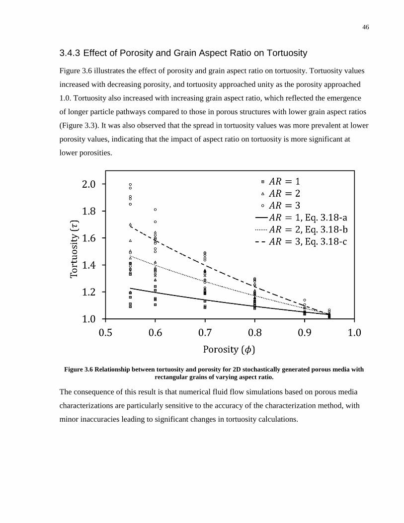
46
3.4.3 Effect of Porosity and Grain Aspect Ratio on Tortuosity
Figure 3.6 illustrates the effect of porosity and grain aspect ratio on tortuosity. Tortuosity values
increased with decreasing porosity, and tortuosity approached unity as the porosity approached
1.0. Tortuosity also increased with increasing grain aspect ratio, which reflected the emergence
of longer particle pathways compared to those in porous structures with lower grain aspect ratios
(Figure 3.3). It was also observed that the spread in tortuosity values was more prevalent at lower
porosity values, indicating that the impact of aspect ratio on tortuosity is more significant at
lower porosities.
Figure 3.6 Relationship between tortuosity and porosity for 2D stochastically generated porous media with
rectangular grains of varying aspect ratio.
The consequence of this result is that numerical fluid flow simulations based on porous media
characterizations are particularly sensitive to the accuracy of the characterization method, with
minor inaccuracies leading to significant changes in tortuosity calculations.
47
3.4.4 Applicability of 2D Model
The applicability of our 2D stochastic modelling results to the results of previous experiments
[51] with similar porous media was examined. The tortuosity values obtained from the MRT
LBM were fit to tortuosity-porosity relations of the following general logarithmic form:
𝜏 = 𝑎 − 𝑏 ln(𝜙), (3.17)
where 𝑎 and 𝑏 are adjusting parameters. Below are the explicit logarithmic tortuosity-porosity
correlations that were found to describe the numerical tortuosity values for a porosity range of
𝜙 ∈ (0.55 − 0.95):
𝜏 = 1.01 − 0.37ln(𝜙), for 𝐴𝑅 = 1 (3.18-a)
𝜏 = 0.99 − 0.80ln(𝜙), for 𝐴𝑅 = 2 (3.18-b)
𝜏 = 0.98 − 1.16ln(𝜙), for 𝐴𝑅 = 3 (3.18-c)
The correlations stated above are also shown in Figure 3.6. As shown in Equations 3.18, it was
found that a ~1 for all three examined aspect ratios, which is in agreement with Equation 3.8
[51,142-145]. The value of 𝑏 was also found to agree with the adjusting parameter, 𝑃, from
Equation 3.8. 𝑃 values are the experimentally-determined adjusting parameters of the 𝜏 − 𝜙
correlation, and 𝑏 values are the adjusting parameters for the numerically-determined 𝜏 − 𝜙
correlations. The b values reported in Equations 3.18 correspond to the experimentally
determined 𝑃 values by Comiti and Renaud [51] (in the range 0.86 to 3.2) for porous media
consisting of parallelepipedal particles of low thickness-to-side ratios with distinct aspect ratios
(for 𝐴𝑅 = 2.27, 𝑃 = 0.86; for 𝐴𝑅 = 4.78, 𝑃 = 1.66; and for 𝐴𝑅 = 9.8, 𝑃 = 3.2). For example, the 𝑃
value for 𝐴𝑅 = 2, can be linearly extrapolated to 𝑃 = 0.78 based on the near-linear relationship
that exists between the 𝑃 and 𝐴𝑅 values reported by Comiti and Renaud [51]. The 𝑃 value of
0.78 agrees with the 𝑏 value of 0.80 (Equation 3.18-b) that was calculated for 𝐴𝑅 = 2 by fitting
Equation 3.17 to the numerical tortuosity values presented here.
Experimentally-determined 𝑃 values reported by Comiti and Renaud [51] as well as the
numerically-determined 𝑏 values from the present work are shown in Figure 3.7. This figure
shows that 𝑏 and 𝑃 values exhibit a near-linear correlation with grain aspect ratio. It can also be
seen that 𝑏 and 𝑃 values are in agreement over the overlapping range of grain aspect ratio.

48
Figure 3.7 Relationship between the experimentally-determined adjusting parameters (𝑷) reported by Comiti
and Renaud [51] and grain aspect ratio as well as the relationship between the numerically-determined
adjusting parameters (𝒃) from the present work and grain aspect ratio. The dashed lines connecting the data
points are only intended to show the trend and do not represent a linear fit.
Based on the agreement between the adjusting parameters in Equations 3.18 and the adjusting
parameters suggested by Comiti and Renaud [51], the tortuosity calculated from 2D stochastic
modelling of porous media with freely overlapping rectangles provides realistic simulations of
porous media with fixed beds of parallelepipedal particles of low thickness-to-side ratio. Such
porous media are relevant to the pulp and paper industry such as wood chips that are used for
paper pulp synthesis [51].
3.5 Conclusions
In this study, the impact of grain aspect ratio on the tortuosity-porosity relationships in porous
media was investigated using an MRT LBM based analysis. To determine the impact of grain
aspect ratio on the tortuosity-porosity relationships, average tortuosity values in 2D
stochastically generated porous media composed of rectangular particles were calculated. It was
shown that tortuosity exhibits an inverse relationship with the porosity that can be expressed in
logarithmic form. The adjusting parameters in the tortuosity-porosity correlation of 𝜏 = 𝑎 −

49
𝑏. ln(𝜙) were calculated. It was also demonstrated that the effect of aspect ratio on the tortuosity
diminishes as the porosity approaches unity. Therefore, it is expected that accurate
characterization of porous media in terms of the grain aspect ratio becomes critical in predicting
tortuosity and resolving fluid flow in low porosity formations.
In addition, it was shown that the tortuosity values from the 2D stochastic domains were in
agreement with the results reported by Comiti and Renaud [51], and therefore expected to be
applicable to similar domains such as fixed beds packed with parallelepipedal particles of low
thickness-to-side ratio, such as wood chips used in the pulp and paper industry. It was also
determined that a minimum of 6, 8 and 10 stochastic simulations were required to calculate the
average tortuosity values in laminar flow (𝑅𝑒 ≪ 1) simulations of our 2D domain for aspect
ratios of 1, 2 and 3, respectively. The work presented here provides a methodology for porous
media researchers to numerically determine tortuosity-porosity correlations that can be validated
with experimentally derived measurements. The methodology presented in this work provides a
useful tool for material designers to tailor the particle arrangements of particles for prescribing
desired tortuosity parameters.

50

51
4 Analytical Tortuosity-porosity Correlations for
Two Deterministic Fractal Geometries3
4.1 Abstract
Naturally-occurring porous media, such as sedimentary rock, rarely consist of mono-sized
particles, but rather tend to consist of wide distributions of particle sizes (poorly-sorted porous
media). In this study, deterministic fractal geometries including a Sierpinski carpet and a slightly
altered version of the Sierpinski carpet with a generator that has a circular inclusion were used to
provide insight into the poorly-sorted porous media found in sedimentary rock. The relationships
between tortuosity and porosity within these fractals were investigated by presenting and
applying a novel mathematical approach. A new correlation between the tortuosity, 𝜏, and
porosity, 𝜙, was found within this Sierpinski carpet (𝜏 =3
2−
𝜙
2), which agrees well with previous
empirical observations reported in the literature. An analytical tortuosity-porosity correlation was
also found within a circular-based Sierpinski carpet (𝜏 = (1 −4
𝜋)𝜙 +
4
𝜋), which is to the best of
the author’s knowledge, the first tortuosity-porosity relationship proposed for the circular-based
Sierpinski carpet.
4.2 Introduction
Tortuosity ,𝜏, is a parameter frequently utilized in continuum models during estimates of
effective flow and transport properties within porous media [54,134]. The concept of tortuosity
was first introduced by Carman [42] in 1937 as a parameter that describes the average elongation
of microscopic fluid flow (particle) pathways in porous media with respect to free flow [55]. In
the subsequent and often cited Kozeny-Carman relationship, tortuosity is used to determine the
permeability, 𝐾, of porous media, as follows [54,134]:
𝐾 =1
𝐶𝐾𝐶.𝜙3
𝑆2𝜏2, (4.1)
where 𝐶𝐾𝐶, 𝜙, and 𝑆 are the Kozeny-Carman constant (shape factor), porosity, and specific
surface area, respectively [155].
3 This chapter is based on a published paper: Ebrahimi Khabbazi A, Hinebaugh J, Bazylak A. Analytical tortuosity–
porosity correlations for Sierpinski carpet fractal geometries, Chaos, Solitons and Fractals 78 (2015) 124 – 133.

52
In the literature, most investigations of tortuosity involve porous media consisting of mono-sized
(same-sized) particles, such as the analytical studies by Yun et al. [59], Yu & Li [60], and Jian-
Long et al. [61] or the numerical studies by Koponen et al. [53,54] and Matyka et al. [47].
However, natural granular porous media (e.g. sedimentary rocks) are rarely mono-sized [44]. It is
noteworthy to mention that even though the structures studied by Koponen et al. [53,54] and
Matyka et al. [47] were constructed by monosized particles, overlapping was allowed, which
could potentially lead to structures of a narrow range of sizes, especially in low porosity systems.
In addition to granular porous media, sometimes fibrous porous materials (e.g. filters and
insulating materials) have wide distributions of fibre diameter (poorly-sorted). Figure 4.1 shows
the schematic of a mono-sized medium and a poorly-sorted granular porous medium. Figure 4.2
shows a scanning electron microscopy (SEM) image of a granular rock sample (Pink Dolomite)
which exhibits wide distributions of particle sizes.
Figure 4.1 Schematic of a (a) well-sorted sedimentary rock versus (b) a poorly-sorted sedimentary rock.

53
Figure 4.2 Microscale (SEM) image of a granular rock sample (Pink Dolomite).
Evidence suggests that natural porous media can be described as a fractal [62,64,156]. There is
even stronger support that surfaces of rock grain and of whole rock samples are fractal [157,158].
Therefore, in the field of porous media, many researchers have used fractals to generate poorly-
sorted porous structures to characterize natural porous media properties or to simulate fluid flow
within porous formations [67-69,159-163]. A fractal is a structure that contains repeating
patterns at every length scale (generation). In theory, fractals can be infinitely self-similar
meaning that they can contain a particular geometric shape (square, circle, etc) in an infinite
range of length scales. Therefore, they can be useful in representing porous materials that contain
wide distributions of particle sizes at various length scales. For instance, the 𝑛𝑡ℎ generation of a
fractal can represent porous media that contain grains of 𝑛 distinct sizes.

54
Figure 4.3 Construction process for the Sierpinski carpet: (a) 0th
generation, (b) 1st generation, (c) 2
nd
generation; as well as for the circular-based Sierpinski carpet: (d) 0th
generation, (e) 1st generation, (f) 2
nd
generation – grey squares represent solid particles.
The Sierpinski carpet (Figure 4.3a-c) is a commonly used fractal [67-69] with a long history of
application to natural porous media [70,71]. The Sierpinski carpet is expected to represent rock
formations particularly at higher generations (lower porosities) where the fractals are less sparse.
Therefore, the fractal can act as an appropriate benchmarking domain for modelling transport in
porous media consisting of wide distributions of particle sizes [71]. Feranie and Latief [69]
applied a square full-walk technique to calculate tortuosity in a 2D fractal model of porous media
constructed of randomized Sierpinski carpets. They reported good agreement with previous work
[53,164] for the porosity range of 𝜙 ∈ (0.3,0.7). Feranie and Latief [69] focused their study on
porous media containing grains of 2 to 4 distinct sizes. Li and Yu [67] estimated tortuosity
through a deterministic Sierpinski carpet using an analytical method and generated the following
exponential relationship between tortuosity and porosity:
𝜏 = (19
18)
ln(𝜙)
ln(8/9). (4.2)

55
An advantage of their model is that it can be applied over a full range of porosities (Sierpinski
carpet generation:𝑛 ∈ {0, 1, 2, … ,∞}). Although Li and Yu’s [67] results diverge from the linear
[53,69] or close-to-linear [165] tortuosity-porosity correlations found by other researchers, theirs
follows the concave trend suggested by many of the works discussed by Ghanbarian et al. [44].
Ghanbarian et al. [44] suggested that the bounds of tortuosity should be 1 at 𝜙 = 1 and should
approach infinity as the porosity approaches some critical value (limiting porosity, which is 0 for
the Sierpinski carpet).
In another study, Lue et al. [68] found the following logarithmic relationship between tortuosity
and porosity for the Sierpinski carpet:
𝜏 = 0.946 − 0.408 ln(𝜙). (4.3)
Four generations of the Sierpinski carpet (𝑛 ∈ {2, 3, 4, 5} or 𝜙 ∈ (0.55 − 0.79)) were considered
in their modelling efforts due to the computational limitations. While previous work provided
great insight into the tortuosity-porosity relationships for low-generation Sierpinski carpets, new
insight is needed for materials that exhibit wider distributions of particle sizes (high-generation
Sierpinski carpet). Since the Sierpinski carpet only features square grains, the effect of grain
shape on the tortuosity-porosity correlation requires further investigation.
An analytical approach for determining tortuosity relationships can be particularly beneficial for
high generations (𝑛 > 6) of fractals where mesh-based numerical approaches can become
computationally prohibitive. High-generation fractal geometries can be equivalent to the porous
media containing grains or pore spaces with substantial variances in size. Figure 4.3 shows an
example of the first 3 generations (𝑛 = 0, 1, and 2) of such geometries, though one can imagine
higher generations can be used to represent wider distributions of particle sizes. For instance, at
𝑛 = 5, the smallest grain is a factor of 1.5 × 10⁻⁴ the size of the largest grain in the domain.
While non-uniform numerical meshes could be applied, at the higher generations required for
low porosity domains, the substantial disparity in length scales could make the numerical models
prohibitively computationally expensive [166]. Therefore, an analytical model is crucial for
tortuosity estimation, particularly when wide distributions of particle sizes exist within the
porous media.

56
In summary, an accurate analytical method is required to study the tortuosity-porosity
correlations in high-generation fractals (porous media with wide distributions of grain sizes).
New correlations are needed to improve estimates of effective flow and transport properties
within such low-porosity formations. Furthermore, it is still unknown how the shape of the grain
may affect the tortuosity-porosity relationships in a Sierpinski carpet type of structure (where the
Sierpinski carpet structure is fixed and only the square grains in the structure are replaced by
other shapes such as circles).
In this study, a new analytical approach was proposed and applied to calculate the tortuosity of
flow within a 2D deterministic Sierpinski carpet. Furthermore, the proposed approach was
applied to calculate the tortuosity of the flow in a round-grained version of the Sierpinski carpet,
the circular-based Sierpinski carpet. In both cases, a linear correlation with a distinct slope
between tortuosity and porosity was found that aligned well with other work [53,69,165].
4.3 Methodology
In this section, the construction process of the used porous media (the Sierpinski carpet and the
circular-based Sierpinski carpet) is presented followed by a description of the proposed
analytical method with detailed mathematical derivation steps:
4.3.1 Geometry
The two geometries used in this study are a Sierpinski carpet (Figure 4.3a-c) as well as a slightly
altered version of the Sierpinski carpet with a generator that has a circular inclusion, hereafter
called the circular-based Sierpinski carpet (Figure 4.3d-f). Figure 4.3a-c shows the construction
of the first three generations (𝑛 = 0, 1, and 2) of the Sierpinski carpet. The 0th
generation, which
is also called the initiator of the Sierpinski carpet, is an empty square (Figure 4.3a). If the 0th
generation is divided into 9 equal square sections and the central section is filled with a solid
square, then the 1st generation is formed (Figure 4.3b). If this process is continued recursively for
the 8 remaining empty squares in the 1st generation, the 2
nd generation is formed (Figure 4.3c).
Higher generations are similarly generated by replicating this process, which can be continued

57
indefinitely. The circular-based Sierpinski carpet is also constructed by following the same rules
as in the Sierpinski carpet generation; however, instead of fully filling the central square with
solid material, a circle is inscribed. Figure 4.3d-f shows the construction of the first three
generations of the circular-based Sierpinski carpet.
4.3.2 Analytical Model
The analytical tortuosity calculations that follow are proposed as an alternative approach to that
presented by Li and Yu [67] for the deterministic Sierpinski carpet. It should be noted that
hydraulic tortuosities have not been calculated in our work. Instead, analytical tortuosities have
been calculated, where straight pathways follow the direction of the macroscopic flux touching
and tracing around the grain boundaries and passing through pore space. In reality, fluid particles
are expected to travel through smoothed streamlines. The simplifying assumptions in our method
can be summarized as below:
(i) the fluid is considered to be arbitrarily compressible,
(ii) vortex generation within the porous media is neglected.
According to the definition of the analytical tortuosity given above, there are some expected
deviations from the hydraulic tortuosity values. Assumption (i) leads to a comparative
underestimation of tortuosity due to artificially straight flow paths in the void regions; the flow
far from the solid particles would have had some curvatures due to the streamlines around the
solid particles in a hydraulic simulation. Assumption (ii), on the other hand, leads to an
overestimation of tortuosity; the neglected vortices would have made a portion of the pores
inaccessible to incoming fluid particles, resulting in less tortuous flow paths (it should be noted
that the particles in the recirculation regions are not considered in tortuosity calculations because
they do not enter or exit the domain). Matyka and Koza [167] showed that the hydraulic
tortuosity is lower than the analytical prediction, which led us to expect that the overestimating
effect of Assumption (ii) dominates the counteracting underestimating effect of Assumption (i).
It should be noted that the straight flow paths resulted from Assumption (i) may not be physical.
Nonetheless, as discussed above, since Assumption (i) and (ii) have counteracting effects on the
tortuosity values, it is expected that the tortuosity values calculated using the presented analytical
approach are physically representative.
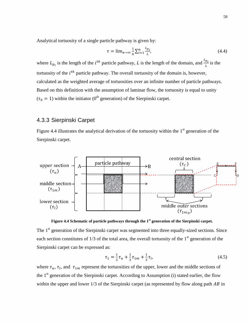
58
Analytical tortuosity of a single particle pathway is given by:
𝜏 = lim𝑛→∞1
𝑛∑
𝐿𝑝𝑖
𝐿
𝑛𝑖=1 , (4.4)
where 𝐿𝑝𝑖 is the length of the 𝑖𝑡ℎ particle pathway, 𝐿 is the length of the domain, and 𝐿𝑝𝑖
𝐿 is the
tortuosity of the 𝑖𝑡ℎ particle pathway. The overall tortuosity of the domain is, however,
calculated as the weighted average of tortuosities over an infinite number of particle pathways.
Based on this definition with the assumption of laminar flow, the tortuosity is equal to unity
(𝜏0 = 1) within the initiator (0th
generation) of the Sierpinski carpet.
4.3.3 Sierpinski Carpet
Figure 4.4 illustrates the analytical derivation of the tortuosity within the 1st generation of the
Sierpinski carpet.
Figure 4.4 Schematic of particle pathways through the 1st generation of the Sierpinski carpet.
The 1st generation of the Sierpinski carpet was segmented into three equally-sized sections. Since
each section constitutes of 1/3 of the total area, the overall tortuosity of the 1st generation of the
Sierpinski carpet can be expressed as:
𝜏1 =1
3𝜏𝑢 +
1
3𝜏1𝑚 +
1
3𝜏𝑙, (4.5)
where 𝜏𝑢, 𝜏𝑙, and 𝜏1𝑚 represent the tortuosities of the upper, lower and the middle sections of
the 1st generation of the Sierpinski carpet. According to Assumption (i) stated earlier, the flow
within the upper and lower 1/3 of the Sierpinski carpet (as represented by flow along path 𝐴𝐵 in

59
Figure 4.4) was straight, and the tortuosity in the upper and lower sections are approximated to
be 𝜏0 (unity). As a result, 𝑡1 can be written as:
𝜏1 =2
3𝜏0 +
1
3𝜏1𝑚. (4.6)
The middle section, however, can be divided further into three more sections: one central and
two outer sections as shown in Figure 4.4. Therefore, the tortuosity in the middle section, 𝜏1𝑚,
can be written as:
𝜏1𝑚 =2
3𝜏1𝑚𝑜
+1
3𝜏𝐶 , (4.7)
where 𝜏1𝑚𝑜 and 𝜏𝐶 represent the tortuosity in the middle outer and the central sections of the 1
st
generation of the Sierpinski carpet. Due to the geometric similarity between the middle outer
sections and the 0th
generation of the Sierpinski carpet, the tortuosity in these sections are
approximated with 𝜏0. The tortuosity in the middle section can be expressed as:
𝜏1𝑚 =2
3𝜏0 +
1
3𝜏𝐶 . (4.8)
This is the point where our approach diverges from the earlier method presented by Li and Yu
[67] as they considered:
𝜏1𝑚 =7
6𝜏1. (4.9)
Combining Equations 4.6 and 4.8 will result in the following expression for the overall tortuosity
of the 1st generation:
𝜏1 =8
9𝜏0 +
1
9𝜏𝐶 . (4.10)
Similarly, for the 2nd
generation, the tortuosity in the upper, lower and the middle outer sections
can be approximated with 𝜏1 and written as:
𝜏2 =8
9𝜏1 +
1
9𝜏𝐶 . (4.11)
In a similar fashion, it follows that the overall tortuosity for the nth
generation is:
𝜏𝑛 =8
9𝜏𝑛−1 +
1
9𝜏𝐶 , (4.12)
which is a recursive expression that can also be written as:

60
𝜏𝑛 =8
9[8
9𝜏𝑛−2 +
1
9𝜏𝑐] +
1
9𝜏𝐶 . (4.13)
If the expression inside the bracket is further expended, it leads to the following formula for the
𝑛𝑡ℎ generation tortuosity:
𝜏𝑛 = (8
9)𝑛
𝜏0 +1
9𝜏𝐶 [(
8
9)𝑛−1
+⋯+ (8
9)1
+ (8
9)0
]. (4.14)
Since 𝜏0 = 1:
𝜏𝑛 = (8
9)𝑛
+1
9𝜏𝐶 ∑ (
8
9)𝑖
.𝑛−1𝑖=0 (4.15)
The summation term in Equation 4.15 can be expressed as:
∑ (8
9)𝑖
𝑛−1𝑖=0 = −9 [(
8
9)𝑛
− 1]. (4.16)
Combining Equation 4.15 and 4.16 results in 𝜏𝑛, written as a function of the generation number,
n:
𝜏𝑛 = (8
9)𝑛
+ 𝜏𝐶 (1 − (8
9)𝑛
). (4.17)
The porosity of a material can also be calculated as the weighted average of the porosities of its
sections:
𝜙𝑛 = (8
9)𝑛
+1
9𝜙𝐶 ∑ (
8
9)𝑖
𝑛−1𝑖=0 , (4.18)
Therefore, the porosity of the Sierpinski carpet fractal and the circular-based Sierpinski carpet
can be calculated using the following expression:
𝜙𝑛 = (8
9)𝑛
+ 𝜙𝐶 (1 − (8
9)𝑛
), (4.19)
where 𝜙𝑐 is the porosity of the central section. After a set of algebraic manipulations of
Equations 4.17 and 4.19, a general form of the tortuosity-porosity correlation can be found for
the fractals with Sierpinski carpet structure:
𝜏𝑛 = [1−𝜏𝐶
1−𝜙𝐶] (𝜙𝑛 − 𝜙𝐶) + 𝜏𝐶. (4.20)

61
As defined above, the tortuosity in the central section, 𝜏𝐶, can be expressed as the average
tortuosity values (over an infinite number of particle pathways around the central grain). Due to
the square grain in the Sierpinski carpet, this is equivalent to the average value of the most and
least tortuous flow paths in this section (CD and EF in Figure 4.4), which is 𝜏𝐶 =2+1
2=
3
2. For
the Sierpinski carpet fractal, 𝜙𝐶 is zero, as the entire centre cell is occupied by the square grain.
Substituting 𝜏𝐶 and 𝜙𝐶 into Equation 4.20 results in the following expression for overall
tortuosity for the nth
generation (valid for 𝜙𝑛 ∈ [0,1]):
𝜏𝑛 =3
2−
𝜙𝑛
2. (4.21)
By substituting 𝜙𝐶 of the Sierpinski carpet (Equation 4.19), the porosity of such porous media
takes on the following form:
𝜙𝑛 = (8
9)𝑛
, (4.22)
4.3.4 Circular-based Sierpinski Carpet
Using the same analogy for the circular-based Sierpinski carpet, the tortuosity of the 𝑛𝑡ℎ
generation of the circular-based Sierpinski carpet will follow the same form as Equation 4.20. To
calculate the tortuosity in the central section, 𝜏𝐶, however, the average tortuosity (over the most
and least tortuous flow paths in the central section) cannot be simply used as it was done for the
Sierpinski carpet analysis. Instead, an infinite number of particle pathways travelling around the
central grain must be considered to calculate the average tortuosity.
Figure 4.5 Schematic of particle pathways through the 1st generation of the circular-based Sierpinski carpet.

62
Due to symmetry, the tortuosity of the central section of the circular-based Sierpinski carpet, 𝜏𝐶,
can be calculated by integrating the tortuosity function (Equation 4.23) of the 𝐴𝐵𝐶 flow path
shown in Figure 4.5 from 0 to 𝑅. The tortuosity function of the 𝐴𝐵𝐶 flow path is given by:
𝜏𝐶(𝜃) =𝐴𝐵 +𝐵𝐶
𝑅=
𝑅(1−cos(𝜃))+𝑅(𝜋
2−𝜃)
𝑅= (1 +
𝜋
2) − (𝜃 + cos(𝜃)), (4.23)
where 𝜃 is the angle ∠𝐵𝑂𝐷 as described in Figure 4.5. To obtain the tortuosity of the central
section, this function has to be integrated along the vertical direction over 0 < 𝜒 < 𝑅 with equal
vertical steps. According to Figure 4.5, angle 𝜃 can be expressed as:
𝜃 = asin (𝜒
𝑅), (4.24)
thus, combining Equations 4.23 and 4.24 leads to the following expression for the tortuosity of
any arbitrary particle pathway in the central section of the circular-based Sierpinski carpet:
𝜏𝐶(𝜒) = (1 +𝜋
2) − [asin (
𝜒
𝑅) + cos (asin (
𝜒
𝑅))]. (4.25)
Integrating 𝜏𝐶(𝜒) over 0 < 𝜒 < 𝑅 will result in the following expression for the average
tortuosity in the central section of the circular-based Sierpinski carpet:
𝜏𝐶 =∫ 𝜏𝐶(𝜒).𝑑𝜒𝑅0
𝑅= 2 −
𝜋
4. (4.26)
Furthermore, one can show that the porosity of the central section in the circular-based Sierpinski
carpet is:
𝜙𝐶 =4𝑅2−𝜋𝑅2
4𝑅2= 1 −
𝜋
4. (4.27)
Substituting 𝜏𝐶 from Equation 4.26 and 𝜙𝐶 from Equation 4.27 back into Equation 4.20, the
tortuosity-porosity correlation for the circular-based Sierpinski carpet is given by:
𝜏𝑛 = (1 −4
𝜋)𝜙𝑛 +
4
𝜋. (4.28)
Furthermore, after substituting 𝜙𝐶 of the circular-based Sierpinski carpet (Equation 4.19), the
porosity of the 𝑛𝑡ℎ generation of the circular-based Sierpinski carpet takes on the following
form:
𝜙𝑛 = 1 −𝜋
4(1 − (
8
9)𝑛
). (4.29)

63
It should be noted that both of the above calculated tortuosity-porosity correlations (Equations
4.21 and 4.28) are applicable across generations of their respective geometries, i.e. 𝑛 ∈
{0, 1, 2, … ,∞}. As a result, their range of validity is 𝜙 ∈ (0,1] for the Sierpinski carpet and
𝜙 ∈ (1 −𝜋
4, 1] for the circular-based Sierpinski carpet. Note that 𝜙 = 0 and 1 −
𝜋
4 are the
limiting porosities for the Sierpinski carpet and the circular-based Sierpinski carpet, where the
limits occur when 𝑛 → ∞.
4.4 Results and Discussion
In this section, the obtained tortuosity-porosity correlations will be compared with existing
tortuosity-porosity relationships in the literature. Two relationships similar to the linear
correlations calculated here have been previously reported by other researchers [53,69,165]:
𝜏 = 1 + 𝑝(1 − 𝜙), (4.30)
𝜏2 = 1 + 𝑞(1 − 𝜙), (4.31)
where 𝑝 and 𝑞 are adjusting parameters. Equation 4.30 was proposed by Feranie and Latief [69]
for the tortuosity in randomized Sierpinski carpets (RSCs) with 𝑝 = 0.799 for the porosity range
of 𝜙 ∈ (0.3 − 0.7). The same form of tortuosity-porosity correlation (Equation 4.30) was one of
the suggested correlations by Koponen et al. [53] after they solved the flow equations for a
porosity range of 𝜙 ∈ [0.5, 1] for randomly placed squares with free overlapping using Lattice
Gas Automata (LGA). Equation 4.31 was determined empirically by Iversen and Jørgensen [165]
for sandy (𝑞 = 2) or clay-silt (𝑞 = 3) sediments over the porosity range of 𝜙 ∈ (0.4 − 0.9). It
should be noted that even though the work by Iversen and Jørgensen [165] was based on
diffusive tortuosities, it should be reasonable to use their results for the verification of analytical
(straight-line based) tortuosity values. According to Ghanbarian et al. [44], in the Sierpinski
carpet (as employed in this work), the straight-line based tortuosity will match the diffusive
tortuosity under the assumptions of steady state and established concentration gradient
conditions.
Regression analyses were performed to find the suitable 𝑝 and 𝑞 that fit to our analytical model.
Since 𝑝 is the adjusting parameter in the linear tortuosity-porosity correlation (Equation 4.30)

64
and our analytical approach also led to a linear tortuosity-porosity correlation, one can use any
number of generations of the analytical results (> 2) in the regression analysis to calculate the
exact value of 𝑝 for both geometries. As for 𝑞, we used 8 and 12 generations of the analytical
results in the regression analyses for the Sierpinski carpet and the circular-based Sierpinski
carpet, respectively. These numbers of generations were selected since 𝑞 is the adjusting
parameter for the Equation 4.31 that has been reported by Iversen and Jørgensen [165] to be only
valid over the approximate porosity range of 𝜙 ∈ (0.4 − 0.9). Our nonlinear regression analyses
involved the Generalized Reduced Gradient (GRG2) algorithm [168]. The error function for the
GRG2 algorithm was defined as the square root of the sum-squared difference between the
tortuosity values from the present study and those generated by Equations 4.30 and 4.31.
Implementing the regression analysis for the Sierpinski carpet, it was found that Equations 4.30
and 4.31 provided a satisfactory fit with 𝑝 = 0.500 and 𝑞 = 1.122. Meanwhile, 𝑝 =4
𝜋− 1 and
𝑞 = 0.583 were found to provide satisfactory fit for the circular-based Sierpinski carpet. 𝑝 and 𝑞
are adjusting parameters obtained by fitting the previously reported tortuosity-porosity
correlations [53,69,165] to our analytically derived tortuosity values. The coefficient of
determination was found to be 1 for Equation 4.30 for both the Sierpinski carpet and the circular-
based Sierpinski carpet. However, the coefficients of determinations were found to be 0.9997
and 0.9992 for Equation 4.31 for the Sierpinski carpet and the circular-based Sierpinski carpet,
respectively.
Our tortuosity-porosity correlations (Equations 4.21 and 4.28) are in agreement with the two
aforementioned correlations (Equations 4.30 and 4.31): each correlation follows a linear trend (as
in Equation 4.21, 4.28, and 4.30) or a close-to-linear trend (as in Equation 4.31). The difference
between our analytically-determined adjusting parameters and those from previous studies can be
attributed to (i) the differing geometry of pore spaces used in each study and (ii) the simplifying
assumptions used in our analytical model. Figure 4.6 provides a comparative view of the
tortuosity values obtained by the present analytical model (Equation 4.21) for the Sierpinski
carpet with those correlations stated above (Equations 4.30 and 4.31) [69,165].

65
Figure 4.6 Analytical tortuosity values of the Sierpinski carpet from present study versus tortuosity values
obtained from previous correlations [69,165] with new adjusting parameters determined through regression
analysis.
Figure 4.7 provides a comparative view of the present analytical model (Equation 4.28) for the
circular-based Sierpinski carpet with previous empirical correlations reported by other
researchers (Equations 4.30 and 4.31) [69,165]. This comparison shows that the same form of
tortuosity-porosity correlations proposed by other researchers [69,165] can still be applied to the
Sierpinski carpet with the modified adjusting parameters. Furthermore, this agreement between
our correlations and the ones reported by others [53,69,165] validates our proposed analytical
approach for estimating tortuosity.

66
Figure 4.7 Analytical tortuosity values of the circular-based Sierpinski carpet from present study versus
tortuosity values obtained from previous correlations [69,165] with new adjusting parameters determined
through regression analysis.
It can be observed from Equation 4.19 that the tortuosity-porosity correlation for any
deterministic fractals with Sierpinski carpet structure has a linear form. In addition, because 𝜏𝐶
and 𝜙𝐶 are constant with respect to any repeating shape, it can be expected that this linear
correlation comes with a distinct slope for any other shaped repeating element in the Sierpinski
carpet structure. Coefficient 𝑝 in Equation 4.30 can be expressed in terms of 𝜏𝐶 and 𝜙𝐶 as
follows:
𝑝 = −1−𝜏𝐶
1−𝜙𝐶. (4.32)
As shown above, the analytical tortuosity-porosity correlations would be linear for any
deterministic fractals that follow the Sierpinski carpet structure regardless of the shape of the
grains (square, circle, etc). This linearity of the analytical tortuosity-porosity correlations may be
counter-intuitive when compared to some tortuosity-porosity correlations presented by
Ghanbarian et al. [44] where tortuosity approached infinity as porosity approached a critical
value. This discrepancy can be attributed to two possible reasons:
(i) The structured nature of the Sierpinski carpet: e.g. however much solid is added to the
domain, the solids do not overlap or touch each other. Therefore, pathway deviations are
local and insignificant. Figure 4.8 provides an example of a highly structured porous
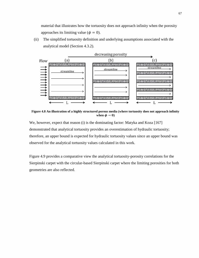
67
material that illustrates how the tortuosity does not approach infinity when the porosity
approaches its limiting value (𝜙 = 0).
(ii) The simplified tortuosity definition and underlying assumptions associated with the
analytical model (Section 4.3.2).
Figure 4.8 An illustration of a highly structured porous media (where tortuosity does not approach infinity
when 𝝓 → 𝟎)
We, however, expect that reason (i) is the dominating factor: Matyka and Koza [167]
demonstrated that analytical tortuosity provides an overestimation of hydraulic tortuosity;
therefore, an upper bound is expected for hydraulic tortuosity values since an upper bound was
observed for the analytical tortuosity values calculated in this work.
Figure 4.9 provides a comparative view the analytical tortuosity-porosity correlations for the
Sierpinski carpet with the circular-based Sierpinski carpet where the limiting porosities for both
geometries are also reflected.

68
Figure 4.9 The analytical tortuosity-porosity correlations for the Sierpinski carpet versus the circular-based
Sierpinski carpet.
As it can be observed, the dashed line representing the tortuosity-porosity correlation for the
Sierpinski carpet covers the entire porosity range of 𝜙 ∈ (0, 1]. This range for the circular-based
Sierpinski carpet is 𝜙 ∈ (1 −𝜋
4, 1]. The lower bounds in both cases indicate the limiting
porosities as Equation 4.18 reduces to 𝜙𝐶 when 𝑛 → ∞. The limiting porosity and the tortuosity-
porosity correlation both vary with the shape of the grain (square to circle), despite the identical
location of the grains in the porous structures (same configurations).
4.5 Conclusions
In this study, a new analytical approach was proposed and applied to calculate tortuosity-porosity
correlations in the Sierpinski carpet (𝜏𝑛 =3
2−
𝜙𝑛
2). A tortuosity-porosity correlation was also
obtained for the circular-based Sierpinski carpet (𝜏𝑛 = (1 −4
𝜋)𝜙𝑛 +
4
𝜋) applicable for the infinite
generation, which would have been computationally prohibitive to obtain numerically. From
Equations 4.21 and 4.28, it is evident that the tortuosity obtained from both geometries exhibited
linear relationships. This observation is in agreement with the trend proposed by Koponen et al.

69
[53] and Feranie and Latief [69]. However, our findings starkly contrast the trend for the
Sierpinski carpet tortuosity presented by Li and Yu [67].
In this work, it was also shown that the limiting porosity and the tortuosity-porosity correlations
in the porous media of the same structure could be impacted by the shape of the grains.
Nonetheless, the linear trend in tortuosity-porosity correlations remained unaffected by the shape
of the grain.
It was shown how the tortuosity values calculated from a 2D analytical model for the Sierpinski
carpet fractal and the circular-based Sierpinski carpet follow a similar correlation (linear or
close-to-linear) proposed by previous researchers. The corresponding adjusting parameters were
then calculated for each structure.
The present model is a conceptual tool which can provide profound insights on how estimates of
effective flow and transport properties for continuum models of low-porosity fractal formations
can be determined. As an extension to this study, it would be helpful to investigate how the
tortuosity values from a 3D analytical model compare to previous studies. Additionally, it would
be interesting to show the dependence of the tortuosity-porosity correlation adjusting parameters
on the rotation of the entire Sierpinski carpet or the individual grains.

70

71
5 Conclusions and Recommendations
In this thesis, LBM and a novel analytical approach were developed for determining continuous
permeability-porosity and tortuosity-porosity relationships in porous media. The numerical tool
has the advantage of being applied to complex domains and boundary conditions. The numerical
model is also a powerful tool for stochastic and parametric studies because the geometry of the
digitally-constructed medium can be varied rapidly and arbitrarily. However, capabilities of
numerical modelling are limited to the available computational resources and therefore,
challenges may arise when encountering geometries with substantial disparity in length scales.
Conversely, analytical tools proved to be highly capable of handling such domains with
substantial disparity in length scales.
5.1 Conclusions and Contributions
In Chapter 2, the permeabilities of two simulated porous structures: periodic arrays of a)
staggered parallel infinite cylinders and b) spheres were calculated using LBM. Using the
numerically calculated permeabilities, 𝐶𝐾𝐶 was modified to enable the the KC equation to
produce permeability values that closely matched the numerical values. It was found that an
algebraic function for 𝐶𝐾𝐶 provided the most accurate prediction of the KC equation for the
geometries examined.
In Chapter 3, stochastic numerical modelling was performed to investigate the impact of the
geometric properties of the individual grains (such as grain aspect ratio) on the tortuosity-
porosity relationships in porous media. It was found that:
tortuosity exhibits an inverse relationship with the porosity that can be expressed in
logarithmic form.
tortuosity increases with increasing grain aspect ratio.
the effect of grain aspect ratio on the tortuosity diminishes as the porosity approaches
unity. Therefore, it is expected that accurate characterization of porous media in terms of
the grain aspect ratio becomes critical in predicting tortuosity and resolving fluid flow in
low porosity formations.

72
a minimum of 6, 8 and 10 stochastic simulations were required to calculate the average
tortuosity values in laminar flow (𝑅𝑒 ≪ 1) simulations of the simulated 2D domains for
aspect ratios of 1, 2 and 3, respectively.
In Chapter 4, a novel analytical approach was proposed and implemented to investigate the
relationships between tortuosity and porosity within the Sierpinski carpet and the circular-based
Sierpinski carpet. It was found that the tortuosity-porosity correlations in such deterministic
fractals are linear and the tortuosity has an upper bound in the limiting porosity. Additionally, it
was found that the value of the limiting porosity and the slope of the linear tortuosity-porosity
correlation could be impacted by the shape of the grain.
In summary, LBM was used in this thesis to study the fluid flow in various forms of porous
media to characterize transport properties such as permeability and tortuosity. This highly-
parallelizable numerical tool has the capability to be used for larger and more complex
geometries. Additionally, a novel analytical approach was introduced and implemented to
characterize tortuosity in fractal geometries. These methodologies can be further utilized to
improve continuous permeability-porosity and tortuosity-porosity relationships for other forms of
porous media. These continuous relationships are critical for continuum-scale fluid simulations
in porous materials.
5.2 Future Work
The following areas of research are recommended for future work:
Reconstructed porous domains from computed tomography (CT) images could be used in
LBM. Domains reconstructed from CT images have the potential to be more
representative of the porous material under investigation.
Parametric studies could be performed using the stochastic modelling approach presented
in Chapter 3. One could determine the impact of parameters, such as: grain shape, grain
orientations, etc. on transport properties (tortuosity, permeability, etc.). This study can
also be extended to incorporate 3D domains.

73
The analytical approach presented in Chapter 4 for calculating tortuosity in fractals can
be further modified and improved based on the results of the numerical tools. One may
use regression analysis to define new adjusting parameters to the analytical correlations
by fitting the analytical correlations to the numerical results. As mentioned earlier,
numerically modelling fractals becomes increasingly difficult as the generation number
increases (due to the substantial disparity in length scales). Therefore, one can only
typically use the first few generations of a fractal for the regression analysis (to inform
analytical correlations). An analytical model modified via a regression analysis could be
representative for high generations of the fractals.

74
References
[1] Dagan G. Statistical theory of groundwater flow and transport: Pore to laboratory, laboratory
to formation, and formation to regional scale. Water Resour.Res. 1986;22(9S):120S-34S.
[2] Blunt MJ. Flow in porous media — pore-network models and multiphase flow. Curr. Opin.
Colloid Inter. Sci. 2001;6(3):197-207.
[3] Doughty C, Pruess K. Modeling supercritical carbon dioxide injection in heterogeneous
porous media. Vadose Zone J. 2004;3(3):837-47.
[4] Strathmann H. Membrane separation processes: current relevance and future opportunities.
AICHE J. 2001;47(5):1077-87.
[5] Djilali N. Computational modelling of polymer electrolyte membrane (PEM) fuel cells:
challenges and opportunities. Energy 2007;32(4):269-80.
[6] Vafai K. Handbook of porous media. 2nd ed. United States: CRC Press; 2005.
[7] Darcy H. Les fontaines publiques de la ville de Dijon. 1st ed. France: Victor Dalmont; 1856.
[8] Vafai K, Tien C. Boundary and inertia effects on flow and heat transfer in porous media.
Int.J.Heat Mass Transfer 1981;24(2):195-203.
[9] Brinkman H. On the permeability of media consisting of closely packed porous particles.
Applied Scientific Research 1949;1(1):81-6.
[10] Phelan FR. Simulation of the injection process in resin transfer molding. Polymer
Composites 1997;18(4):460-76.
[11] Abrate S. Resin flow in fiber preforms. Appl.Mech.Rev. 2002;55(6):579-99.
[12] Khanafer K, Vafai K. The role of porous media in biomedical engineering as related to
magnetic resonance imaging and drug delivery. Heat and mass transfer 2006;42(10):939-53.
[13] Ai L, Vafai K. A coupling model for macromolecule transport in a stenosed arterial wall.
Int.J.Heat Mass Transfer 2006;49(9):1568-91.
[14] Pan C, Hilpert M, Miller CT. Pore-scale modeling of saturated permeabilities in random
sphere packings. Physical Review E 2001;64(6):066702.
[15] Masch FD, Denny KJ. Grain size distribution and its effect on the permeability of
unconsolidated sands. Water Resour.Res. 1966;2(4):665-77.

75
[16] Lu W, Tung K, Hwang K. Fluid flow through basic weaves of monofilament filter cloth.
Text.Res.J. 1996;66(5):311-23.
[17] Tung K, Shiau J, Chuang C, Li Y, Lu W. CFD analysis on fluid flow through multifilament
woven filter cloths. Sep.Sci.Technol. 2002;37(4):799-821.
[18] Wang L, Afsharpoya B. Modeling fluid flow in fuel cells using the lattice-Boltzmann
approach. Math.Comput.Simul. 2006;72(2):242-8.
[19] Nathan Matthew Lane. Numerical studies of flow in porous media using an unstructured
approach. United States: Southeastern Louisiana University; 2011.
[20] Audigane P, Gaus I, Czernichowski-Lauriol I, Pruess K, Xu T. Two-dimensional reactive
transport modeling of CO2 injection in a saline aquifer at the Sleipner site, North Sea. Am. J. Sci.
2007;307(7):974-1008.
[21] Izgec O, Demiral B, Bertin H, Akin S. CO2 injection into saline carbonate aquifer
formations I: Laboratory investigation. Transp. Porous. Med. 2008;72(1):1-24.
[22] Ji C, Ahmadi G and Smith DH. Experimental and computational studies of fluid flow
phenomena in carbon dioxide sequestration in brine and oil fields. WA, USA: First National
Conference on Carbon Sequestration; 2001.
[23] Juanes R, Spiteri EJ, Orr Jr. FM, Blunt MJ. Impact of relative permeability hysteresis on
geological CO2 storage. Water Resour. Res. 2006;42:W12418.
[24] Oldenburg C, Benson S. CO2 injection for enhanced gas production and carbon
sequestration. Villahermosa, Mexico: SPE International Petroleum Conference and Exhibition;
2002.
[25] Ramstad T, Idowu N, Nardi C, Øren PE. Relative permeability calculations from two-phase
flow simulations directly on digital images of porous rocks. Transp. Porous. Med. 2011:1-18.
[26] Carman P. The determination of the specific surface of powders. J.Soc.Chem.Ind.Trans
1938;57:225.
[27] Wiggins EJ, Campbell WB, Maass O. Determination of the specific surface of fibrous
materials. Canadian Journal of Research 1939;17(10):318-24.
[28] Sullivan R. Specific surface measurements on compact bundles of parallel fibers.
J.Appl.Phys. 1942;13(11):725-30.
[29] Brown J. Determination of the exposed specific surface of pulp fibers from air permeability
measurements. Tappi 1950;33(3):130-7.
[30] Langmuir I. Report on smokes and filters. Office of Scientific Research and Development
No 865, Ser No 353, Filtration of aerosols and the development of filter materials 1942.

76
[31] Rodebush W, Langmuir I, LaMer V. Filtration of Aerosols and the Development of Filter
Materials. 0.SRD Report 1942;865.
[32] Happel J. Viscous flow relative to arrays of cylinders. AICHE J. 1959;5(2):174-7.
[33] Sparrow E, Loeffler A. Longitudinal laminar flow between cylinders arranged in regular
array. AICHE J. 1959;5(3):325-30.
[34] Drummond J, Tahir M. Laminar viscous flow through regular arrays of parallel solid
cylinders. Int.J.Multiphase Flow 1984;10(5):515-40.
[35] Kuwabara S. The forces experienced by randomly distributed parallel circular cylinders or
spheres in a viscous flow at small Reynolds numbers. Journal of the physical society of Japan
1959;14(4):527-32.
[36] Hasimoto H. On the periodic fundamental solutions of the Stokes equations and their
application to viscous flow past a cubic array of spheres. J.Fluid Mech. 1959;5(2):317-28.
[37] Sangani A, Acrivos A. Slow flow through a periodic array of spheres. Int.J.Multiphase Flow
1982;8(4):343-60.
[38] Spielman L, Goren SL. Model for predicting pressure drop and filtration efficiency in
fibrous media. Environ.Sci.Technol. 1968;2(4):279-87.
[39] Jackson GW, James DF. The hydrodynamic resistance of hyaluronic acid and its
contribution to tissue permeability. Biorheology 1982;19(1/2):317-30.
[40] Koponen A, Kandhai D, Hell'en E, Alava M, Hoekstra A, Kataja M, et al. Permeability of
Three-Dimensional Random Fiber Webs. Phys.Rev.Lett. 1998;80(4):716-9.
[41] Pinela J, Kruz S, Miguel A, Reis A and Aydin M. Permeability-Porosity Relationship
Assessment by 2D Numerical Simulations. Proceedings; 2005.
[42] Carman PC. Fluid flow through granular beds. T.I.Chem.Eng.Lond. 1937;15:150-66.
[43] Panda MN, Lake LW. Estimation of single-phase permeability from parameters of particle-
size distribution. AAPG.Bull. 1994;78(7):1028-39.
[44] Ghanbarian B, Hunt AG, Ewing RP, Sahimi M. Tortuosity in porous media: a critical
review. Soil Sci. Soc. Am. J. 2013;77(5):1461-77.
[45] Sahimi M. Flow phenomena in rocks: from continuum models to fractals, percolation,
cellular automata, and simulated annealing. Rev. Mod. Phys. 1993;65(4):1393-534.
[46] Clennell MB. Tortuosity: a guide through the maze. Geol. Soc. London Spec. Publ.
1997;122(1):299-344.

77
[47] Matyka M, Khalili A, Koza Z. Tortuosity-porosity relation in porous media flow. Phys. Rev.
E 2008;78(2):026306.
[48] Adler PM. Porous Media: Geometry and Transports. 1st ed. United States: Butterworth-
Heinemann; 1992.
[49] Epstein N. On tortuosity and the tortuosity factor in flow and diffusion through porous
media. Chem. Eng. Sci. 1989;44(3):777-9.
[50] D. Pech. Etude de la perméabilité de lits compressibles constitués de copeaux de bois
partiellement destructurés. France: Institut polytechnique de Grenoble; 1984.
[51] Comiti J, Renaud M. A new model for determining mean structure parameters of fixed beds
from pressure drop measurements: application to beds packed with parallelepipedal particles.
Chem. Eng. Sci. 1989;44(7):1539-45.
[52] Mauret E, Renaud M. Transport phenomena in multi-particle systems—I. Limits of
applicability of capillary model in high voidage beds-application to fixed beds of fibers and
fluidized beds of spheres. Chem. Eng. Sci. 1997;52(11):1807-17.
[53] Koponen A, Kataja M, Timonen J. Tortuous flow in porous media. Phys. Rev. E
1996;54(1):406.
[54] Koponen A, Kataja M, Timonen J. Permeability and effective porosity of porous media.
Phys. Rev. E 1997;56(3):3319-25.
[55] Duda A, Koza Z, Matyka M. Hydraulic tortuosity in arbitrary porous media flow. Phys.
Rev. E 2011;84(3):036319.
[56] Nabovati A, Sousa ACM. Fluid flow simulation in random porous media at pore-level using
the lattice Boltzmann method. JESTEC. 2007;2(3):226-37.
[57] Du Plessis JP, Masliyah JH. Flow through isotropic granular porous media. Transp. Porous
Media 1991;6(3):207-21.
[58] Ahmadi MM, Mohammadi S, Hayati AN. Analytical derivation of tortuosity and
permeability of monosized spheres: A volume averaging approach. Phys. Rev. E
2011;83(2):026312.
[59] Yun M, Yu B, Zhang B, Huang M. A geometry model for tortuosity of streamtubes in
porous media with spherical particles. Chin. Phys. Lett. 2005;22(6):1464-7.
[60] Yu B, Li J. A geometry model for tortuosity of flow path in porous media. Chin. Phys. Lett.
2004;21(8):1569-71.
[61] Jian-Long K, Xue-Ming T, Hai-Yan Z, Hang-Jun L, Feng-Min W, You-Sheng X, et al.
Tortuosity for streamlines in porous media. Chin. Phys. B 2012;21(4):044701.

78
[62] Bayles GA, Klinzing GE, Chiang SH. Fractal mathematics applied to flow in porous
systems. Part.Part.Syst.Char. 1989;6(1‐4):168-75.
[63] Pape H, Clauser C, Iffland J. Variation of permeability with porosity in sandstone diagenesis
interpreted with a fractal pore space model. Pure Appl.Geophys. 2000;157(4):603-20.
[64] Katz A, Thompson A. Fractal sandstone pores: implications for conductivity and pore
formation. Phys.Rev.Lett. 1985;54(12):1325.
[65] Tosatti E, Pietrelli L. Fractals in physics. The Netherlands: Elsevier; 2012.
[66] Rawls W, Brakensiek D, Logsdon S. Predicting saturated hydraulic conductivity utilizing
fractal principles. Soil Sci.Soc.Am.J. 1993;57(5):1193-7.
[67] Li J, Yu B. Tortuosity of flow paths through a Sierpinski carpet. Chin. Phys. Lett.
2011;28(3):034701.
[68] Luo L, Yu B, Cai J, Zeng X. Numerical simulation of tortuosity for fluid flow in two-
dimensional pore fractal models of porous media. Fractals 2014;22(04).
[69] Feranie S, Latief FD. Tortuosity–porosity relationship in two-dimensional fractal model of
porous media. Fractals 2013;21(02).
[70] Garrison Jr JR, Pearn WC, von Rosenberg D. The fractal Menger sponge and Sierpinski
carpet as models for reservoir rock/pore systems: I.; Theory and image analysis of Sierpinski
carpets. In Situ;(United States) 1992;16(4):351-406.
[71] Doughty C, Karasaki K. Flow and transport in hierarchically fractured rock. J. Hydrol
2002;263(1):1-22.
[72] Ebrahimi Khabbazi A, Bazylak A. Lattice Boltzmann Simulation of Tortuous Flow within
Stochastic Porous Media and the Examination of the Tortuosity-Porosity Relationship. United
States: The 224th Electrochemical Society Meeting; 2013.
[73] Ebrahimi Khabbazi A, Ellis JS and Bazylak A. Hydrodynamic Modeling of CO2-Saturated
Brine Injection in Geologic Formations for Carbon Sequestration Using the Lattice Boltzmann
Method. United States: AMSE 5th International Conference on Energy Sustainability; 2011.
[74] Ellis JS, Ebrahimi Khabbazi A and Bazylak A. Characterization of a Two-phase Pore-scale
Network Model of Supercritical Carbon Dioxide Transport within Brine-filled Porous Media.
United States: AMSE 5th International Conference on Energy Sustainability; 2011.
[75] Ebrahimi Khabbazi A, Ellis JS and Bazylak A. Lattice Boltzmann Simulation of
Supercritical Carbon Dioxide in Brine-Saturated Underground Porous Media. Canada: The 219th
Electrochemical Society Meeting; 2011.

79
[76] Ellis JS, Ebrahimi Khabbazi A and Bazylak A. Characterization of Supercritical Carbon
Dioxide Transport within a Brine-filled Porous Media using a Two-phase Pore Network Model.
Canada: The 219th Electrochemical Society Meeting; 2011.
[77] Hocking G, Forbes L. The lens of freshwater in a tropical island–2D withdrawal.
Comput.Fluids 2004;33(1):19-30.
[78] Dong B, Yan Y, Li W, Song Y. Lattice Boltzmann simulation of viscous fingering
phenomenon of immiscible fluids displacement in a channel. Comput.Fluids 2010;39(5):768-79.
[79] Zerai B, Saylor BZ, Kadambi JR, Oliver MJ, Mazaheri AR, Ahmadi G, et al. Flow
characterization through a network cell using particle image velocimetry. Transp.Porous Media
2005;60(2):159-81.
[80] Parseval YD, Pillai K, Advani S. A simple model for the variation of permeability due to
partial saturation in dual scale porous media. Transp.Porous Media 1997;27(3):243-64.
[81] Nghiem L, Shrivastava V, Kohse B, Hassam M, Yang C. Simulation and optimization of
trapping processes for CO2 storage in saline aquifers. J.Can.Pet.Technol. 2010;49(8):15-22.
[82] Jerauld G, Salter S. The effect of pore-structure on hysteresis in relative permeability and
capillary pressure: pore-level modeling. Transp. Porous. Med. 1990;5(2):103-51.
[83] Bryant S, Blunt M. Prediction of relative permeability in simple porous media. Phys. Rev. A
1992;46(4):2004.
[84] Dana E, Skoczylas F. Gas relative permeability and pore structure of sandstones. Int.J.Rock
Mech.Min.Sci. 1999;36(5):613-25.
[85] Xu P, Yu B. Developing a new form of permeability and Kozeny-Carman constant for
homogeneous porous media by means of fractal geometry. Adv.Water Resour. 2008;31(1):74-81.
[86] Tomadakis MM, Robertson TJ. Viscous permeability of random fiber structures:
Comparison of electrical and diffusional estimates with experimental and analytical results.
J.Compos.Mater. 2005;39(2):163-88.
[87] Gebart BR. Permeability of unidirectional reinforcements for RTM. J.Composite Mater.
1992;26(8):1100-33.
[88] Walsh JB, Brace WF. The effect of pressure on porosity and the transport properties of rock.
J.Geophys.Res. 1984;89(B11):9425-31.
[89] Mavko G, Nur A. The effect of a percolation threshold in the Kozeny‐Carman relation.
Geophysics 1997;62:1480-2.
[90] Bourbié T, Coussy O, Zinszner B. Acoustics of porous media. 1st ed. France: Gulf
Publishing Co.; 1987.

80
[91] Fishman Z, Hinebaugh J, Bazylak A. Microscale Tomography Investigations of
Heterogeneous Porosity Distributions of PEMFC GDLs. J.Electrochem.Soc.
2010;157(11):B1643-50.
[92] Kuo CW, Perrin JC, Benson SM. Simulation studies of effect of flow rate and small scale
heterogeneity on multiphase flow of CO2 and brine. Energy Procedia 2011;4:4516-23.
[93] Pan C, Luo LS, Miller CT. An evaluation of lattice Boltzmann schemes for porous medium
flow simulation. Comput. Fluids 2006;35(8-9):898-909.
[94] Schneider K. Numerical simulation of the transient flow behaviour in chemical reactors
using a penalisation method. Comput.Fluids 2005;34(10):1223-38.
[95] Hamidi M, Sabbagh-Yazdi SR. Modeling of 2D density-dependent flow and transport in
porous media using finite volume method. Comput.Fluids 2008;37(8):1047-55.
[96] Jaffre J. Approximation of a diffusion-convection equation by a mixed finite element
method: application to the water flooding problem. Comput.Fluids 1980;8(2):177-88.
[97] L. Axner. High performance computational hemodynamics with the lattice Boltzmann
method. Amsterdam, The Netherlands: University of Amsterdam; 2007.
[98] Chen S, Doolen GD. Lattice Boltzmann method for fluid flows. Annu.Rev.Fluid Mech.
2003;30(1):329-64.
[99] Ahrenholz B, Tölke J, Krafczyk M. Lattice-Boltzmann simulations in reconstructed
parametrized porous media. Int. J. Comput. Fluid D. 2006;20(6):369-77.
[100] Ahrenholz B, Niessner J, Helmig R, Krafczyk M. Pore-scale determination of parameters
for macroscale modeling of evaporation processes in porous media. Water Resour.Res.
2011;47(7):W07543.
[101] Tölke J. Lattice Boltzmann simulations of binary fluid flow through porous media.
Philosophical Transactions of the Royal Society of London.Series A: Mathematical, Physical and
Engineering Sciences 2002;360(1792):535-45.
[102] Yablecki J, Hinebaugh J, Bazylak A. Effect of Liquid Water Presence on PEMFC GDL
Effective Thermal Conductivity. J.Electrochem.Soc. 2012;159(12):F805-9.
[103] Yablecki J, Nabovati A, Bazylak A. Modeling the effective thermal conductivity of an
anisotropic gas diffusion layer in a polymer electrolyte membrane fuel cell. J.Electrochem.Soc.
2012;159(6):B647-53.
[104] Sukop MC, Or D. Invasion percolation of single component, multiphase fluids with lattice
Boltzmann models. Physica B: Condensed Matter 2003;338(1-4):298-303.

81
[105] Yan Y, Zu Y, Dong B. LBM, a useful tool for mesoscale modelling of single-phase and
multiphase flow. Appl.Therm.Eng. 2010.
[106] Gokaltun S, McDaniel D. Multiple-relaxation-time lattice Boltzmann method for
multiphase flows with high density and viscosity ratios. Phoenix, AZ, USA: WM2010
Conference; 2010.
[107] Huang H, Wang L, Lu X. Evaluation of three lattice Boltzmann models for multiphase
flows in porous media. Comput. Math. Appl. 2010.
[108] Guta L, Sundar S. Navier-Stokes-Brinkman system for interaction of viscous waves with a
submerged porous structure. Tamkang.J.Math 2010;41(3):217-43.
[109] Succi S. The lattice Boltzmann equation for fluid dynamics and beyond. 1st ed. United
States: Oxford University Press; 2001.
[110] Shardt O, Mitra SK, Derksen J. Lattice Boltzmann simulations of pinched flow
fractionation. Chem.Eng.Sci. 2012;75:106-19.
[111] Reider MB, Sterling JD. Accuracy of discrete-velocity BGK models for the simulation of
the incompressible Navier-Stokes equations. Comput.Fluids 1995;24(4):459-67.
[112] Bhatnagar PL, Gross EP, Krook M. A model for collision processes in gases. I. Small
amplitude processes in charged and neutral one-component systems. Phys. Rev. 1954;94(3):511.
[113] Guo Z, Shi B, Wang N. Lattice BGK model for incompressible Navier-Stokes equation.
J.Comput.Phys. 2000;165(1):288-306.
[114] Qian YH, d'Humieres D, Lallemand P. Lattice BGK models for Navier-Stokes equation.
Europhys.Lett. 1992;17(6):479-84.
[115] Latt J, Chopard B, Malaspinas O, Deville M, Michler A. Straight velocity boundaries in
the lattice Boltzmann method. Phys. Rev. E 2008;77(5):056703.
[116] Dullien FAL. Two‐phase flow in porous media. Chem. Eng. Technol. 1988;11(1):407-24.
[117] Nabovati A, Llewellin EW, Sousa A. Through-thickness permeability prediction of three-
dimensional multifilament woven fabrics. Composites Part A: Applied Science and
Manufacturing 2010;41(4):453-63.
[118] Kang Q, Lichtner PC, Viswanathan HS, Abdel-Fattah AI. Pore-scale modeling of reactive
transport involved in geologic CO2 sequestration. Transp. Porous. Med. 2010;82(1):197-213.
[119] Kumar A, Noh M, Pope G, Sepehrnoori K, Bryant S and Lake L. Reservoir simulation of
CO2 storage in deep saline aquifers. Tusla, Oklahoma, USA: SPE/DOE Symposium on Improved
Oil Recovery; 2004.
82
[120] Ziegler DP. Boundary conditions for lattice Boltzmann simulations. J.Stat.Phys.
1993;71(5):1171-7.
[121] Ginzbourg I, Adler P. Boundary flow condition analysis for the three-dimensional lattice
Boltzmann model. Journal de Physique II 1994;4(2):191-214.
[122] d’Humières D, Ginzburg I. Viscosity independent numerical errors for Lattice Boltzmann
models: from recurrence equations to “magic” collision numbers. Comput.Math.Appl.
2009;58(5):823-40.
[123] Davies L, Dollimore D. Theoretical and experimental values for the parameter k of the
Kozeny-Carman equation, as applied to sedimenting suspensions. J.Phys.D 2000;13(11):2013.
[124] Kyan CP, Wasan D, Kintner R. Flow of single-phase fluids through fibrous beds. Ind. Eng.
Chem. Fundam. 1970;9(4):596-603.
[125] Happel J, Brenner H, Moreau R. Low Reynolds number hydrodynamics: with special
applications to particulate media (mechanics of fluids and transport processes). MA, USA:
Kluwer Boston; 1983.
[126] Lasdon L, Waren A. Generalized reduced gradient software for linearly and nonlinearly
constrained problems. 1st ed. United States: Graduate School of Business, University of Texas at
Austin; 1977.
[127] Kozeny J. Ueber kapillare Leitung des Wassers im Boden. Stizungsber Akad Wiss Wien
1927;136:271-306.
[128] Kaviany M. Principles of heat transfer in porous media. New York: Springer; 1995.
[129] Thorat IV, Stephenson DE, Zacharias NA, Zaghib K, Harb JN, Wheeler DR. Quantifying
tortuosity in porous Li-ion battery materials. J. Power Sources 2009;188(2):592-600.
[130] Dixit AB, McDougall SR, Sorbie KS and Buckley JS. Pore scale modelling of wettability
effects and their influence of oil recovery. United States: SPE/DOE 10th symposium on
improved oil recovery; 1996.
[131] Oren PE. Pore-scale network modelling of waterflood residual oil recovery by immiscible
gas flooding. United States: SPE/DOE Improved Oil Recovery Symposium; 1994.
[132] Nabovati A, Hinebaugh J, Bazylak A, Amon CH. Effect of porosity heterogeneity on the
permeability and tortuosity of gas diffusion layers in polymer electrolyte membrane fuel cells. J.
Power Sources 2014;248:83-90.
[133] Kapadia S, Anderson WK, Burdyshaw C. Channel shape optimization of solid oxide fuel
cells using advanced numerical techniques. Comput. Fluids 2011;41(1):41-50.

83
[134] Nabovati A, Sousa ACM. Fluid flow simulation in random porous media at pore level
using lattice Boltzmann method. JESTEC. 2009;2(3):226-37.
[135] Childs EC. An introduction to the physical basis of soil water phenomena. 1st ed. United
States: John Wiley & Sons; 1969.
[136] Tindall JA, Kunkel JR, Anderson DE. Unsaturated zone hydrology for scientists and
engineers. 1st ed. United States: Prentice Hall; 1999.
[137] Wong PZ. Conductivity, permeability, and electrokinetics. Experimental methods in the
physical sciences: Elsevier; 1999, p. 119-159.
[138] Archie GE. The electrical resistivity log as an aid in determining some reservoir
characteristics. Pet. Tech. 1942;5:54-62.
[139] Satterfield CN, Sherwood TK. The role of diffusion in catalysis. 1st ed. United States:
Addison-Wesley; 1963.
[140] Greenkorn RA. Flow phenomena in porous media: fundamentals and applications in
petroleum, water and food production. 1st ed. United States: Marcel Dekker; 1983.
[141] Shen L, Chen Z. Critical review of the impact of tortuosity on diffusion. Chem. Eng. Sci.
2007;62(14):3748-55.
[142] Weissberg HL. Effective Diffusion Coefficient in Porous Media. J. Appl. Phys.
1963;34(9):2636-9.
[143] Tsai DS, Strieder W. Effective Conductivities of Random Fiber Beds. Chem. Eng.
Commun. 1986;40(1-6):207-18.
[144] Ho F, Striender W. A variational calculation of the effective surface diffusion coefficient
and tortuosity. Chem. Eng. Sci. 1981;36(2):253-8.
[145] Barrande M, Bouchet R, Denoyel R. Tortuosity of porous particles. Anal. Chem.
2007;79(23):9115-21.
[146] Mussa A, Asinari P, Luo LS. Lattice Boltzmann simulations of 2D laminar flows past two
tandem cylinders. J. Comput. Phys. 2009;228(4):983-99.
[147] Razzaghian M, Pourtousi M and Darus AN. Simulation of flow in lid driven cavity by
MRT and SRT. Thailand: International Conference on Mechanical and Robotics Engineering;
2012.
[148] Martinez WL, Martinez AR. Computational statistics handbook with MATLAB. 2nd ed.
United States: CRC press; 2007.
84
[149] Sukop MC, Thorne DT. Lattice Boltzmann modeling: An introduction for geoscientists
and engineers. 1st ed. Germany: Springer-Verlag Berlin Heidelberg; 2006.
[150] Chen L, Zhang L, Kang Q, Viswanathan HS, Yao J, Tao W. Nanoscale simulation of shale
transport properties using the lattice Boltzmann method: permeability and diffusivity. Sci. Rep.
2015;5:1-8.
[151] A. Nabovati. Pore level simulation of single and two phase flow in porous media using
lattice Boltzmann method. Canada: University of New Brunswick; 2009.
[152] Durst F, Ray S, Ünsal B, Bayoumi OA. The development lengths of laminar pipe and
channel flows. J. Fluid. Eng. 2005;127(6):1154-60.
[153] Ebrahimi Khabbazi A, Ellis JS, Bazylak A. Developing a new form of the Kozeny-Carman
parameter for structured porous media through lattice-Boltzmann modeling. Comput. Fluids
2013;75:35-41.
[154] Kueny JL, Binder G. Viscous flow over backward facing steps—an experimental
investigation. In: Morgan K, Periaux J, Thomasset F, editors. Analysis of laminar flow over a
backward facing step. 1st ed. Germany: Vieweg+Teubner Verlag; 1984, p. 32-47.
[155] Gauvin R, Trochu F, Lemenn Y, Diallo L. Permeability measurement and flow simulation
through fiber reinforcement. Polym. Compos. 1996;17(1):34-42.
[156] Turcotte D. Fractals and fragmentation. Journal of Geophysical Research: Solid Earth
(1978–2012) 1986;91(B2):1921-6.
[157] Orford J, Whalley W. The use of the fractal dimension to quantify the morphology of
irregular‐shaped particles. Sedimentology 1983;30(5):655-68.
[158] Avnir D, Farin D, Pfeifer P. Molecular fractal surfaces. Nature 1984;308(5956):261-3.
[159] Cai J, Yu B. Prediction of maximum pore size of porous media based on fractal geometry.
Fractals 2010;18(04):417-23.
[160] Perfect E, Gentry R, Sukop M, Lawson J. Multifractal Sierpinski carpets: Theory and
application to upscaling effective saturated hydraulic conductivity. Geoderma 2006;134(3):240-
52.
[161] Xu Y, Dong P. Fractal approach to hydraulic properties in unsaturated porous media.
Chaos. Soliton. Fract. 2004;19(2):327-37.
[162] Vidales A, Miranda E. Fractal porous media: Relations between macroscopic properties.
Chaos. Soliton. Fract. 1996;7(9):1365-9.
[163] Hunt A. Percolative transport in fractal porous media. Chaos. Soliton. Fract.
2004;19(2):309-25.

85
[164] Boudreau BP. The diffusive tortuosity of fine-grained unlithified sediments.
Geochim.Cosmochim.Acta 1996;60(16):3139-42.
[165] Iversen N, Jørgensen BB. Diffusion coefficients of sulfate and methane in marine
sediments: Influence of porosity. Geochim.Cosmochim.Acta 1993;57(3):571-8.
[166] Chapra SC, Canale RP. Numerical methods for engineers. Sixth ed. New York, NY:
McGraw-Hill; 2009.
[167] Matyka M, Koza Z. How to calculate tortuosity easily? AIP Conf. Proc. 2012;1453:17-22.
[168] Lasdon L, Waren A. Generalized reduced gradient software for linearly and nonlinearly
constrained problems. Austin, Texas, USA: Graduate School of Business, University of Texas;
1977.

86
Appendix I
This appendix is intended to provide more data for validation purposes in order to help in the
reproduction of the work:
Case 1. Poiseuille flow between two parallel plates
In the first validation step, a simulation of Poiseuille flow between two parallel plates was
performed, similar to what Durst et al. [152] have performed. For the validation purposes, the
developing velocity profile was obtained from our MRT model and compared it to the one
obtained from our previously published SRT method [153]. An excellent agreement between
these two models was demonstrated in Figure A-1 and Figure A-2. Secondly, the entry length
calculated from our MRT model was compared to the model proposed by Durst et al. [152].
The parameters used in the MRT model are presented in the table below:
Table A-3. List of physical properties and model parameters
Physical properties Relaxation parameters
Domain length, 𝒏𝒙 = 𝟒𝟎𝟎 𝑠1 = 0
Domain height, 𝒏𝒚 = 𝟒𝟏 𝑠2 = 𝑠3 =
1
𝜏
Inlet Velocity, 𝑼𝒊𝒏 = 𝟎. 𝟎𝟐 𝑠4 = 0
Density, 𝝆𝒐𝒖𝒕 = 𝟏. 𝟎 𝑠5 = 𝑠7 = 8
(2𝜏 − 1)
8𝜏 − 1
Relaxation time, 𝝉 = 𝟎. 𝟖 𝑠6 = 0
Reynolds number, 𝑹𝒆 = 𝟕. 𝟖 𝑠8 = 𝑠9 =
1
𝜏

87
Figure A-10. Developing velocity profile computed by the MRT LBM.
Figure A-11. Developing velocity profile computed by the SRT LBM.
As shown in Figures A-1 and A-2, and as it was expected from the literature, the maximum
velocity occurred at the centreline and it reached to 1.5 times of the inlet velocity (according to
the analytical solution for Poiseuille problem between two parallel plates) at its fully developed

88
condition. The maximum velocity was used as a measure to determine the entry length. Based on
a widely-used criterion, entry length is defined as where the maximum (centreline) velocity
reaches to 99% of its analytical value for fully developed flow. Beyond the entry length, the flow
is called fully-developed. Figure A-3 shows how the entry length was calculated in our model.
Figure A-12. Centreline velocity development along the channel.
Durst et al. [152] has proposed the equation below for the entry length:
𝐿𝑒
𝐷= [(0.631)1.6 + (0.0442𝑅𝑒)1.6]
1
1.6, (A-1)
where 𝐿𝑒 , 𝐷 and 𝑅𝑒 are entry length, height of the channel (spacing between two parallel plates)
and the flow Reynolds number, respectively. Durst et al. [152] (Equation A-1) estimates a value
of 𝐿𝑒
𝐷= 0.77 and our MRT LBM predicts a value of
𝐿𝑒
𝐷= 0.81 for the entry length of the
channel.
Case 2. Flow over backward-facing step
The second case in our validation process was a flow over backward-facing step. This flow is
widely used for validation purposes by numerical modellers. At this step, our results obtained
from the LB simulations was compared with the ones measured experimentally by Kueny et
al.[154]. Figure A-4 shows the geometry used in our simulations as well as setup used in the
experiment performed by Kueny et al. [154]. Tables A-2 and A-3 list experimental conditions in
Kueny’s experiment and simulation parameters in our MRT model.

89
Figure A-13. Schematic of the backward-facing step used in our model.
Table A-4. Experimental conditions used by Kueny et al. [154]
Channel/flow parameters
Value
Upstream height 𝒉
2cm
Downstream height 𝑯
3cm
Step Height 𝒉𝒔 = 𝑯 − 𝒉
1cm
Maximal velocity 𝑼𝑴𝒂𝒙
7.23 cm/s
Reynolds number 𝑹𝒆 =𝑼𝑴𝒂𝒙𝒉𝒔
𝝊
50
Table A-5. Numerical model parameters
Upstream Channel
Length, 𝑻𝒙
100 Inlet Velocity, 𝑼𝒊𝒏
0.111
Step Height, 𝑻𝒚 30 Density, 𝜌 1.0
Domain length, 𝒏𝒙
370 Relaxation time, 𝜏
0.8
Domain height, 𝒏𝒚
92 Reynolds number, 𝑅𝑒
50
Uin
Pouth
H
hs

90
Numerical model parameters were set to replicate the experimental conditions, such as 𝑅𝑒 = 50:
𝑅𝑒 =𝑈𝑀𝑎𝑥ℎ𝑠
𝜐=
3
2𝑈𝑖𝑛ℎ𝑠
1
3(𝜏−0.5)
=3
2(0.111)(30)
1
3(0.8−0.5)
≈ 50. (A-2)
Figure A-5 shows the velocity profiles for the flow over the backward-facing experiment with
𝑅𝑒 = 50 which is in agreement with the experimentally-determined representative velocity
profiles obtained by Kueny et al. [154] (Figure A-6).
Figure A-14. Velocity profile for the flow with 𝐑𝐞 = 50.

91
Figure A-15. Velocity profile (𝐑𝐞 = 50) from the experimental work by Kueny et al. [154].

92
In addition to the velocity profile, a comparison between the streamline patterns obtained from
the LB model and the ones reported by Kueny et al. [154] was performed. Figures A-7 and A-8
show an excellent agreement between the numerical and experimental results. For example, the
dimensionless length of the separation region is calculated to be approximately 3 in both
numerical and experimental studies presented here:
Figure A-7. Streamline patterns (𝐑𝐞= 50) obtained by the MRT LBM.
Figure A-8. Streamline patterns (𝐑𝐞 = 50) from the experimental work by Kueny et al. [154].
Summary
A multiple-relaxation time (MRT) lattice-Boltzmann model (LBM) was developed and validated
with two experiments: (i) Poiseuille flow between two parallel plates, and (ii) laminar flow over
backward-facing step. In the first case, the developing velocity profile of a Poiseuille flow
0 1 2 3 4 5 6 7 8
1
2
3
x/hs
y/h
s

93
between two parallel plates was shown. It was shown that the maximum centreline velocity was
equal to its analytical value (3
2𝑈𝑖𝑛). Furthermore, the entry length obtained from the LB
simulations was compared to the entry length estimated by an empirical equation proposed by
Durst et al. [152] and the results showed agreement (𝐿𝑒
𝐷= 0.81 from the LBM vs.
𝐿𝑒
𝐷= 0.77 from
the empirical equation). In the second experiment, the velocity profiles and the streamline
patterns obtained from our numerical method were compared to the ones from an experimental
study by Kueny et al. [154]. An excellent agreement between the results was observed. For
instance, the dimensionless length of the recirculation zone was found to be equal to
approximately 3 in both studies.

94
Appendix II
This Appendix is intended to provide implementations of the LBM method in various case
scenarios. In general, an LB model goes through the following steps:
Initialize the variables, do the unit conversion
Initialize the domain using the macroscopic parameters
Calculate equilibrium from initialized macroscopic domain
Initialize 𝑓 values on each node
Perform collision on each node
Perform streaming on each node
Set boundary conditions
Calculate macroscopic parameters on each node
Calculate 𝑓𝑒𝑞 on each node
If not converged, repeat steps from collision step …
Below is my detailed step-by-step implementation of SRT LBM for D2Q9:
1. Initialization and defining parameters
ex = [ 1 0 -1 0 1 -1 -1 1 0 ] ; %D2Q9 lattice parameters ey = [ 0 1 0 -1 1 1 -1 -1 0 ] ; w = [ 1/9 1/9 1/9 1/9 1/36 1/36 1/36 1/36 4/9 ] ; cs = 1/sqrt(3) ; % Cs sound speed
Uinitial = 0.000 ; % Uinitial in lattice Units Vinitial = 0.000 ; % Vinitial in lattice Units Rhoinitial = 1.0; % Rhoinitial in lattice Units Tau = 0.80 ; % Tau - Relaxation time
Gx = 1e-4 ; % Body force in lattice units in x direction Gy = 0 ; % Body force in lattice units in y direction dx = 1e-4 ; % dx is 1 in lattice units, which is equal to 1e-4
meters in physical units dt = 1e-5 ; % dt is 1 in lattice units, which is equal to 1e-5
seconds in physical units Utol = 1e-4 ; % Tolerance of U for convergence, if Residual is
smaller than this value, the code is converged Vtol = 1e-4 ; % Tolerance of V Uresidual = 100 ; % set to a huge value for the first iteration, Vresidual = 100 ; % set to a huge value for the first iteration,

95
%define the parameters f = zeros(nx,ny,9); ftemp= zeros(nx,ny,9); feq = zeros(nx,ny,9); U = zeros(nx,ny); V = zeros(nx,ny); Uold = zeros(nx,ny); Vold = zeros(nx,ny); Rho = zeros(nx,ny);
%%%%%%%%%%%%%%%%%%%
% Initialization macroscopic parameters U(:,:) = Uinitial ; V(:,:) = Vinitial ; Rho(:,:) = Rhoinitial ; Uold = U ; Vold = V ;
2. Calculating equilibrium distribution function
for J = 1 : ny for I = 1 : nx for a = 1 : 9 feq(I,J,a) = w(a) * Rho(I,J) * ( 1.0 +
3.0*(ex(a)*U(I,J)+ey(a)*V(I,J)) ... + 9.0/2.0*(
ex(a)*U(I,J)+ey(a)*V(I,J))^2 ... - 3.0/2.0*( U(I,J)^2 +
V(I,J)^2 ) ) ; end end end
3. Collision step
% Body force implementation, Approach 1 g = w .* 1 .* (Gx .* ex + Gy .* ey) ./ cs^2 ; % as everything is in lattice
units, dt is set equal to 1
for J = 1 : ny for I = 1 : nx if isfluid(I,J)==1 for a = 1 : 9 temp = f(I,J,a) - ( f(I,J,a) - feq(I,J,a) ) / Tau +
g(a) ; % Collison on each site, for each direction f(I,J,a) = temp ; end end end end

96
4. Streaming step
% set periodic boundary conditions on both sides for J = 1 : ny if (J>1) JN = J - 1 ; else JN = ny ; % in periodic boundary condition in the y direction,
the row before the first row is the last row end
if (J<ny) JP = J + 1 ; else JP = 1 ; % in periodic boundary condition in the y direction,
the row after the last row is the first row end
for I = 1 : nx if (I>1) IN = I - 1 ; else IN = nx ; %in periodic boundary condition in the x
direction, the column before the first column is the last column end
if (I<nx) IP = I + 1 ; else IP = 1 ; % in periodic boundary condition in the x
direction, the column after the last column is the first column end
ftemp(IP,J ,1) = f(I,J,1) ; % 8 distributions sitting on
node(I,J) flies to 8 neighboring nodes for the next time step ftemp(I ,JP,2) = f(I,J,2) ; ftemp(IN,J ,3) = f(I,J,3) ; ftemp(I ,JN,4) = f(I,J,4) ; ftemp(IP,JP,5) = f(I,J,5) ; ftemp(IN,JP,6) = f(I,J,6) ; ftemp(IN,JN,7) = f(I,J,7) ; ftemp(IP,JN,8) = f(I,J,8) ; ftemp(I ,J ,9) = f(I,J,9) ; % the distribution at the center,
(0,0), stays untouched end end
f = ftemp ; % Update the distribution values
5. Bounce-back solid wall boundary treatment
for J = 1 : ny for I = 1 : nx if isfluid(I,J)==0

97
temp = f(I,J,1) ; % directions of particles are switched
to ensure zero velocity in all directions f(I,J,1) = f(I,J,3) ; f(I,J,3) = temp ;
temp = f(I,J,2) ; f(I,J,2) = f(I,J,4) ; f(I,J,4) = temp ;
temp = f(I,J,5) ; f(I,J,5) = f(I,J,7) ; f(I,J,7) = temp ;
temp = f(I,J,6) ; f(I,J,6) = f(I,J,8) ; f(I,J,8) = temp ; end end end
6. Calculation of macroscopic parameters
Rhotemp = 0 ; % a temporary variable to calculate summation MomtempX = 0 ; MomtempY = 0 ; for J = 1 : ny for I = 1 : nx if isfluid(I,J) == 1 for a = 1 : 9 Rhotemp = Rhotemp + f(I,J,a) ; MomtempX = MomtempX + f(I,J,a)*ex(a) ; % Momentum in x
direction MomtempY = MomtempY + f(I,J,a)*ey(a) ; % Momentum in y
direction end Rho(I,J) = Rhotemp ; % Macroscopic density U(I,J) = MomtempX /Rho(I,J) ; % Macroscopic velocity in x
direction V(I,J) = MomtempY /Rho(I,J) ; % Macroscopic velocity in y
direction Rhotemp = 0 ; MomtempX = 0 ; MomtempY = 0 ; end end end

98
Our implementation of the MRT LBM was based on the SRT LBM presented above except that
the transformation matrix, 𝑀, relaxation rate matrix, ��, and the moments, 𝑚, were implemented
as below:
%%%%%%%%%%%%%%%%%%%Transformation Matrix %%%%%%%%%% M = [ 1 , 1 , 1 , 1 , 1 , 1 , 1 , 1 , 1 ; -1 , -1 , -1 , -1 , 2 , 2 , 2 , 2 , -4 ; -2 , -2 , -2 , -2 , 1 , 1 , 1 , 1 , 4 ; 1 , 0 , -1 , 0 , 1 , -1 , -1 , 1 , 0 ; -2 , 0 , 2 , 0 , 1 , -1 , -1 , 1 , 0 ; 0 , 1 , 0 , -1 , 1 , 1 , -1 , -1 , 0 ; 0 , -2 , 0 , 2 , 1 , 1 , -1 , -1 , 0 ; 1 , -1 , 1 , -1 , 0 , 0 , 0 , 0 , 0 ; 0 , 0 , 0 , 0 , 1 , -1 , 1 , -1 , 0 ];
invM = inv(M) ; tau = 0.8 ; s_e = 1/tau ; s_eps = 1/tau ; s_niu = 1/tau ; s_q = 8.0 * (2-s_niu)/(8-s_niu) ;
S = diag( [0.0 , s_e , s_eps , 0.0 , s_q , 0.0 , s_q , s_niu , s_niu],0 ) ;
niu = (tau - 0.5) / 3.0 ; zeta = (1/s_e - 0.5) / 6.0 ;
Flow between parallel plates in MRT LBM
Below is an implementation of the MRT LBM to model flow between parallel plates. Figure A-
10 and A-12 can be obtained from the following code. Furthermore, inlet and outlet mass flow
rates are calculated to ensure the continuity is satisfied:
clear all
for Uin = 0.02 : 0.04 : 0.1
nx = 400 ; ny = 41 ;
ex = [ 1 0 -1 0 1 -1 -1 1 0 ] ; ey = [ 0 1 0 -1 1 1 -1 -1 0 ] ; w = [ 1/9 1/9 1/9 1/9 1/36 1/36 1/36 1/36 4/9 ] ;
Vin = 0 ; Rhoout = 1.0 ;

99
Uinitial = Uin ; Vinitial = 0.000 ; Rhoinitial = Rhoout;
cs = 1/sqrt(3) ; Gx = 0.0 ; Gy = 0.0 ; dx = 1e-4 ; dt = 1e-5 ; Utol = 1e-3 ; Vtol = 1e-3 ; Uresidual = 100 ; Vresidual = 100 ;
f = zeros (nx,ny,9); ftemp = zeros (nx,ny,9); feq = zeros (nx,ny,9); U = zeros (nx,ny); V = zeros (nx,ny); Uold = zeros (nx,ny); Vold = zeros (nx,ny); Rho = zeros (nx,ny);
isfluid = ones(nx,ny); isfluid(:,1) = 0 ; isfluid(:,ny) = 0 ;
M = [ 1 , 1 , 1 , 1 , 1 , 1 , 1 , 1 , 1 ; -1 , -1 , -1 , -1 , 2 , 2 , 2 , 2 , -4 ; -2 , -2 , -2 , -2 , 1 , 1 , 1 , 1 , 4 ; 1 , 0 , -1 , 0 , 1 , -1 , -1 , 1 , 0 ; -2 , 0 , 2 , 0 , 1 , -1 , -1 , 1 , 0 ; 0 , 1 , 0 , -1 , 1 , 1 , -1 , -1 , 0 ; 0 , -2 , 0 , 2 , 1 , 1 , -1 , -1 , 0 ; 1 , -1 , 1 , -1 , 0 , 0 , 0 , 0 , 0 ; 0 , 0 , 0 , 0 , 1 , -1 , 1 , -1 , 0 ];
invM = inv(M) ; tau = 0.8 ; s_e = 1/tau ; s_eps = 1/tau ; s_niu = 1/tau ; s_q = 8.0 * (2-s_niu)/(8-s_niu) ;
S = diag( [0.0 , s_e , s_eps , 0.0 , s_q , 0.0 , s_q , s_niu , s_niu],0 ) ;
niu = (tau - 0.5) / 3.0 ; zeta = (1/s_e - 0.5) / 6.0 ;
U(:,:) = Uinitial ; V(:,:) = Vinitial ; Rho(:,:) = Rhoinitial ; for J = 1 : ny for I = 1 : nx if isfluid(I,J)==0 U(I,J) = 0 ;

100
V(I,J) = 0 ; end end end
Jx = Rho .* U ; Jy = Rho .* V ; e = -2 * Rho + 3.0 * ( Jx.^2 + Jy.^2) ; eps= Rho - 3.0 * (Jx.^2 + Jy.^2) ; qx = - Jx ; qy = - Jy ; Pxx = Jx.^2 - Jy.^2 ; Pxy = Jx.*Jy ;
meq(:,:,1) = Rho ; meq(:,:,2) = e ; meq(:,:,3) = eps ; meq(:,:,4) = Jx ; meq(:,:,5) = qx ; meq(:,:,6) = Jy ; meq(:,:,7) = qy ; meq(:,:,8) = Pxx ; meq(:,:,9) = Pxy ;
for J = 1 : ny for I = 1 : nx meq_temp(1) = meq(I,J,1) ; meq_temp(2) = meq(I,J,2) ; meq_temp(3) = meq(I,J,3) ; meq_temp(4) = meq(I,J,4) ; meq_temp(5) = meq(I,J,5) ; meq_temp(6) = meq(I,J,6) ; meq_temp(7) = meq(I,J,7) ; meq_temp(8) = meq(I,J,8) ; meq_temp(9) = meq(I,J,9) ; feq(I,J,:) = invM * meq_temp' ; end end
f = feq ; m = meq ;
g = w .* 1 .* (Gx .* ex + Gy .* ey) ./ cs^2 ;
Loop_counter = 1 ;
while Loop_counter <100 || Uresidual > Utol
Rhotemp = 0 ; MomtempX = 0 ; MomtempY = 0 ; for J = 1 : ny for I = 1 : nx if isfluid(I,J) == 1 for a = 1 : 9

101
Rhotemp = Rhotemp + f(I,J,a) ; MomtempX = MomtempX + f(I,J,a)*ex(a) ; MomtempY = MomtempY + f(I,J,a)*ey(a) ; end Rho(I,J) = Rhotemp ; U(I,J) = MomtempX /Rho(I,J) ; V(I,J) = MomtempY /Rho(I,J) ; Rhotemp = 0 ; MomtempX = 0 ; MomtempY = 0 ; end end end
Jx = Rho .* U ; Jy = Rho .* V ; e = -2 * Rho + 3.0 * ( Jx.^2 + Jy.^2) ; eps= Rho - 3.0 * ( Jx.^2 + Jy.^2) ; qx = - Jx ; qy = - Jy ; Pxx = Jx.^2 - Jy.^2 ; Pxy = Jx.*Jy ;
meq(:,:,1) = Rho ; meq(:,:,2) = e ; meq(:,:,3) = eps ; meq(:,:,4) = Jx ; meq(:,:,5) = qx ; meq(:,:,6) = Jy ; meq(:,:,7) = qy ; meq(:,:,8) = Pxx ; meq(:,:,9) = Pxy ;
for J = 1 : ny for I = 1 : nx tempf(1) = f (I,J,1) ; tempf(2) = f (I,J,2) ; tempf(3) = f (I,J,3) ; tempf(4) = f (I,J,4) ; tempf(5) = f (I,J,5) ; tempf(6) = f (I,J,6) ; tempf(7) = f (I,J,7) ; tempf(8) = f (I,J,8) ; tempf(9) = f (I,J,9) ;
tempm = M * tempf' ; m(I,J,:) = tempm ; end end
for J = 1 : ny for I = 1 : nx if isfluid(I,J)==1 dm(1) = m(I,J,1)-meq(I,J,1) ; dm(2) = m(I,J,2)-meq(I,J,2) ; dm(3) = m(I,J,3)-meq(I,J,3) ; dm(4) = m(I,J,4)-meq(I,J,4) ;

102
dm(5) = m(I,J,5)-meq(I,J,5) ; dm(6) = m(I,J,6)-meq(I,J,6) ; dm(7) = m(I,J,7)-meq(I,J,7) ; dm(8) = m(I,J,8)-meq(I,J,8) ; dm(9) = m(I,J,9)-meq(I,J,9) ;
temp = invM * S * dm' + g' ; for a = 1 : 9 f(I,J,a) = f(I,J,a) - temp(a) ; end
end end end
for J = 1 : ny if J > 1 JN = J - 1 ; else JN = ny ; end if J<ny JP = J + 1 ; else JP = 1 ; end
for I = 2 : nx-1 IN = I - 1 ; IP = I + 1 ;
ftemp(I ,J ,1) = f(IN,J , 1) ; ftemp(I ,J ,2) = f(I ,JN, 2) ; ftemp(I ,J ,3) = f(IP,J , 3) ; ftemp(I ,J ,4) = f(I ,JP, 4) ; ftemp(I ,J ,5) = f(IN,JN, 5) ; ftemp(I ,J ,6) = f(IP,JN, 6) ; ftemp(I ,J ,7) = f(IP,JP, 7) ; ftemp(I ,J ,8) = f(IN,JP, 8) ; ftemp(I ,J ,9) = f(I ,J , 9) ; end
I = 1 ; IP = I + 1 ; ftemp(I,J,2) = f( I ,JN, 2 ) ; ftemp(I,J,3) = f( IP,J , 3 ) ; ftemp(I,J,4) = f( I ,JP, 4 ) ; ftemp(I,J,6) = f( IP,JN, 6 ) ; ftemp(I,J,7) = f( IP,JP, 7 ) ; ftemp(I,J,9) = f( I ,J , 9 ) ; Rho(I,J) = ( ftemp(I,J,9)+ftemp(I,J,2)+ftemp(I,J,4)+ 2.0*(
ftemp(I,J,3)+ftemp(I,J,6)+ftemp(I,J,7) ) ) /(1-Uin) ; ftemp(I,J,1) = ftemp(I,J,3)+2.0/3.0* Rho(I,J)*Uin ; ftemp(I,J,5) = 0.5 *( Rho(I,J)*Uin/3.0 + Rho(I,J)*Vin - ftemp(I,J,2) +
ftemp(I,J,4) + 2*ftemp(I,J,7) ) ;

103
ftemp(I,J,8) = 0.5 *( Rho(I,J)*Uin/3.0 - Rho(I,J)*Vin + ftemp(I,J,2) -
ftemp(I,J,4) + 2*ftemp(I,J,6) ) ;
I = nx ; IN = I - 1 ; ftemp(I,J,1) = f( IN,J ,1 ) ; ftemp(I,J,2) = f( I ,JN,2 ) ; ftemp(I,J,4) = f( I ,JP,4 ) ; ftemp(I,J,5) = f( IN,JN,5 ) ; ftemp(I,J,8) = f( IN,JP,8 ) ; ftemp(I,J,9) = f( I ,J ,9 ) ; Rho(I,J) = Rhoout ; UofPout(J) = -1 + ( 2*(ftemp(I,J,1)+ftemp(I,J,5)+ftemp(I,J,8)) +
ftemp(I,J,2) + ftemp(I,J,4) + ftemp(I,J,9) ) / Rho(I,J) ; ftemp(I,J,3) = ftemp(I,J,1) - 2.0/3.0*Rho(I,J)*UofPout(J) ; ftemp(I,J,6) = -Rho(I,J)*UofPout(J)/6.0 + (ftemp(I,J,4)-ftemp(I,J,2))
/ 2.0 + ftemp(I,J,8) ; ftemp(I,J,7) = -Rho(I,J)*UofPout(J)/6.0 + (ftemp(I,J,2)-ftemp(I,J,4))
/ 2.0 + ftemp(I,J,5) ; end
f = ftemp ;
for J = 1 : ny for I = 1 : nx if isfluid(I,J)==0
tempo = f(I,J,1) ; f(I,J,1) = f(I,J,3) ; f(I,J,3) = tempo ;
tempo = f(I,J,2) ; f(I,J,2) = f(I,J,4) ; f(I,J,4) = tempo ;
tempo = f(I,J,5) ; f(I,J,5) = f(I,J,7) ; f(I,J,7) = tempo ;
tempo = f(I,J,6) ; f(I,J,6) = f(I,J,8) ; f(I,J,8) = tempo ; end end end
if mod(Loop_counter,100)==0 Uresidual = 0 ; Vresidual = 0 ;
for J = 1 : ny for I = 1 : nx if abs(U(I,J)) > 0 Uresidual = Uresidual + abs( (U(I,J)-Uold(I,J))/ U(I,J) ); end

104
if abs(V(I,J)) > 0 Vresidual = Vresidual + abs ((V(I,J)-Vold(I,J))/ V(I,J) ); end
end end Uold = U ; Vold = V ;
fprintf(' Iteration = %i, Uresidual = %f \n', Loop_counter, Uresidual) end Loop_counter = Loop_counter + 1 ; end
save (['Uin', num2str(100*Uin)]) end
figure hold on box on grid on xlabel('U/Uin') ylabel('Channel height') yaxis = [1/ny:1/ny:1]; plot(U(300,:)/Uin,yaxis,'b','linewidth',2)
Re = Uin*(ny-2)/niu;
IMFR = 0; %Inlet Mass Flow Rate for J = 1 : ny IMFR = IMFR + Rho(1,J)*U(1,J); end IMFR;
OMFR = 0; %Outlet Mass Flow Rate for J = 1 : ny OMFR = OMFR + Rho(nx,J)*U(nx,J); end OMFR;
abs(OMFR - IMFR)/IMFR

105
Checking for continuity (i.e. ��𝒊𝒏 ≈ ��𝒐𝒖𝒕):
The reader is advised to benchmark the following data with the above code prior to endeavoring
to use the code for further studies. Inlet and outlet mass flow rates were calculated for 3 distinct
inlet velocities (corresponding to 3 Reynolds numbers). In all cases, it was shown that the mass
was conserved (��𝑖𝑛 ≈ ��𝑜𝑢𝑡):
𝑼𝒊𝒏(𝒎/𝒔) 𝑹𝒆 |��𝒊𝒏− ��𝒐𝒖𝒕|/��𝒊𝒏
𝟎. 𝟎𝟐 7.8 2.8 × 10⁻⁶ 𝟎. 𝟎𝟔 23.4 3.0 × 10⁻⁶ 𝟎. 𝟏 39 2.6 × 10⁻⁶
Simulation of flow in a staggered array of parallel cylinders using SRT LBM
Below is an implementation of the SRT LBM to model fluid flow in a staggered array of parallel
cylinders. Figure 2.7 can be obtained from the following model. Furthermore, inlet and outlet
mass flow rates are calculated for various porosities to ensure the continuity is satisfied:
clear all NOgrid = 3*48 ; nx = 1*NOgrid ; ny = 1*NOgrid ;
Radius=NOgrid/48*14.5; Gx=NOgrid/48*48; Gy=NOgrid/48*24; Centrex0=0; Centrey0=0;
ex = [ 1 0 -1 0 1 -1 -1 1 0 ] ; ey = [ 0 1 0 -1 1 1 -1 -1 0 ] ; w = [ 1/9 1/9 1/9 1/9 1/36 1/36 1/36 1/36 4/9 ] ; cs = 1/sqrt(3) ;
Uinitial = 0.000 ; Vinitial = 0.000 ; Rhoinitial = 1.0; RhoP = 1041.3; RhoL = 1.0; ROin = 1.0005; RO = 1.0 ; meu = 6.025e-4; Nu = meu/RhoP; Tau = 1.0 ; NuL = (Tau-0.5)/3;
dx = 48e-5/NOgrid ; dt = NuL/Nu*dx*dx;

106
Utol = 1e-3 ; Vtol = 1e-3 ; Uresidual = 100 ; Vresidual = 100 ;
f = zeros(nx,ny,9); ftemp= zeros(nx,ny,9); feq = zeros(nx,ny,9); U = zeros(nx,ny); V = zeros(nx,ny); Uold = zeros(nx,ny); Vold = zeros(nx,ny); Rho = zeros(nx,ny);
U(:,:) = Uinitial ; V(:,:) = Vinitial ; Rho(:,:) = Rhoinitial ; Rho(nx, 1:ny) = RO ; Uold = U ; Vold = V ;
isfluid = ones(nx,ny); isfluid(:,1) = 1 ; isfluid(:,ny) = 1 ;
for mm = 0 : ny/Gy Centrey = Centrey0 + mm*Gy;
for nn = 0 : nx/Gx if (mod(mm,2)==1) Centrex = Centrex0+(nn-0.5)*Gx; else Centrex = Centrex0+nn*Gx; end
for J = 1 : ny for I = 1 : nx if sqrt((I-(Centrex))^2+(J-Centrey)^2)< Radius isfluid(I,J) = 0; end end end
end end
for J = 1 : ny for I = 1 : nx if isfluid(I,J)==0 U(I,J) = 0 ; V(I,J) = 0 ; end end end

107
for J = 1 : ny for I = 1 : nx for a = 1 : 9 feq(I,J,a) = w(a) * Rho(I,J) * ( 1.0 +
3.0*(ex(a)*U(I,J)+ey(a)*V(I,J)) ... + 9.0/2.0*( ex(a)*U(I,J)+ey(a)*V(I,J))^2 ... - 3.0/2.0*( U(I,J)^2 + V(I,J)^2 ) ) ; end end end
f = feq ;
Loop_counter = 1 ;
while Loop_counter <100 || Uresidual > Utol %|| Vresidual>Vtol
for J = 1 : ny for I = 1 : nx if isfluid(I,J)==1 for a = 1 : 9 temp = f(I,J,a) - ( f(I,J,a) - feq(I,J,a) ) / Tau ; %
f(I,J,a) = temp ; end end end end
for J = 1 : ny if (J>1) JN = J - 1 ; else JN = ny ; end
if (J<ny) JP = J + 1 ; else JP = 1 ; end
for I = 1 : nx IN = I - 1 ; IP = I + 1 ;
if (I==1) ftemp(IP,J ,1) = f(I,J,1) ; ftemp(I ,JP,2) = f(I,J,2) ; ftemp(I ,JN,4) = f(I,J,4) ; ftemp(IP,JP,5) = f(I,J,5) ; ftemp(IP,JN,8) = f(I,J,8) ; ftemp(I ,J ,9) = f(I,J,9) ;
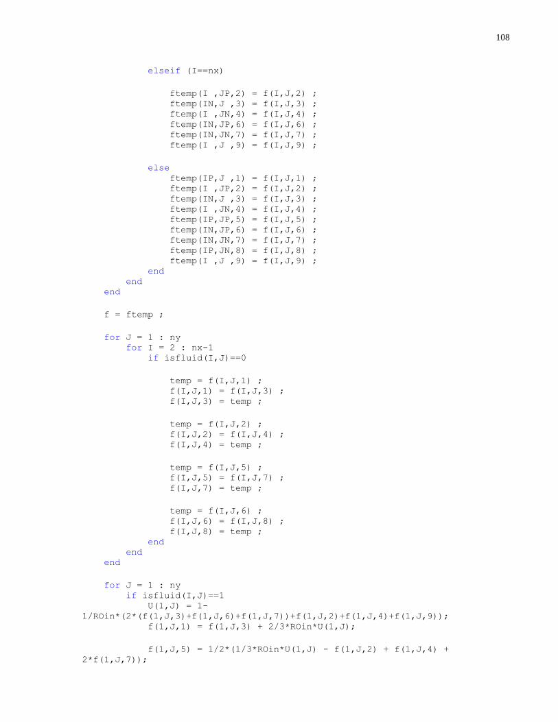
108
elseif (I==nx)
ftemp(I ,JP,2) = f(I,J,2) ; ftemp(IN,J ,3) = f(I,J,3) ; ftemp(I ,JN,4) = f(I,J,4) ; ftemp(IN,JP,6) = f(I,J,6) ; ftemp(IN,JN,7) = f(I,J,7) ; ftemp(I ,J ,9) = f(I,J,9) ;
else ftemp(IP,J ,1) = f(I,J,1) ; ftemp(I ,JP,2) = f(I,J,2) ; ftemp(IN,J ,3) = f(I,J,3) ; ftemp(I ,JN,4) = f(I,J,4) ; ftemp(IP,JP,5) = f(I,J,5) ; ftemp(IN,JP,6) = f(I,J,6) ; ftemp(IN,JN,7) = f(I,J,7) ; ftemp(IP,JN,8) = f(I,J,8) ; ftemp(I ,J ,9) = f(I,J,9) ; end end end
f = ftemp ;
for J = 1 : ny for I = 2 : nx-1 if isfluid(I,J)==0
temp = f(I,J,1) ; f(I,J,1) = f(I,J,3) ; f(I,J,3) = temp ;
temp = f(I,J,2) ; f(I,J,2) = f(I,J,4) ; f(I,J,4) = temp ;
temp = f(I,J,5) ; f(I,J,5) = f(I,J,7) ; f(I,J,7) = temp ;
temp = f(I,J,6) ; f(I,J,6) = f(I,J,8) ; f(I,J,8) = temp ; end end end
for J = 1 : ny if isfluid(I,J)==1 U(1,J) = 1-
1/ROin*(2*(f(1,J,3)+f(1,J,6)+f(1,J,7))+f(1,J,2)+f(1,J,4)+f(1,J,9)); f(1,J,1) = f(1,J,3) + 2/3*ROin*U(1,J);
f(1,J,5) = 1/2*(1/3*ROin*U(1,J) - f(1,J,2) + f(1,J,4) +
2*f(1,J,7));

109
f(1,J,8) = 1/2*(1/3*ROin*U(1,J) + f(1,J,2) - f(1,J,4) +
2*f(1,J,6)); end end
for J = 1 : ny if isfluid(I,J)==1 U(nx,J) = -1 +
1/RO*(2*(f(nx,J,1)+f(nx,J,5)+f(nx,J,8))+f(nx,J,2)+f(nx,J,4)+f(nx,J,9)); f(nx,J,3) = f(nx,J,1) - 2/3*RO*U(nx,J); f(nx,J,6) = 1/2*(-1/3*RO*U(nx,J)-f(nx,J,2)+f(nx,J,4)+2*f(nx,J,8)); f(nx,J,7) = 1/2*(-1/3*RO*U(nx,J)+f(nx,J,2)-f(nx,J,4)+2*f(nx,J,5)); end end
for J = 1 : ny-1 if (isfluid(1,J)==0 && isfluid(1,J+1)==1) f(1,J,1) = f(1,J,3) ; f(1,J,2) = f(1,J,4) ; f(1,J,5) = f(1,J,7) ; f(1,J,6) = 1/2*(ROin -
(f(1,J,9)+f(1,J,1)+f(1,J,2)+f(1,J,3)+f(1,J,4)+f(1,J,5)+f(1,J,7))) ; f(1,J,8) = 1/2*(ROin -
(f(1,J,9)+f(1,J,1)+f(1,J,2)+f(1,J,3)+f(1,J,4)+f(1,J,5)+f(1,J,7))) ; end end
for J = 1 : ny-1 if (isfluid(1,J)==0 && isfluid(1,J+1)==0) f(1,J,1) = f(1,J,3) ; f(1,J,4) = f(1,J,2) ; f(1,J,8) = f(1,J,6) ; f(1,J,5) = 1/2*(ROin -
(f(1,J,9)+f(1,J,1)+f(1,J,2)+f(1,J,3)+f(1,J,4)+f(1,J,6)+f(1,J,8))) ; f(1,J,7) = 1/2*(ROin -
(f(1,J,9)+f(1,J,1)+f(1,J,2)+f(1,J,3)+f(1,J,4)+f(1,J,6)+f(1,J,8))) ; end end
for J = 1 : ny-1 if (isfluid(nx,J)==0 && isfluid(nx,J+1)==0) f(nx,J,3) = f(nx,J,1) ; f(nx,J,4) = f(nx,J,2) ; f(nx,J,7) = f(nx,J,5) ; f(nx,J,6) = 1/2*(RO-
(f(nx,J,9)+f(nx,J,1)+f(nx,J,2)+f(nx,J,3)+f(nx,J,4)+f(nx,J,5)+f(nx,J,7))) ; f(nx,J,8) = 1/2*(RO-
(f(nx,J,9)+f(nx,J,1)+f(nx,J,2)+f(nx,J,3)+f(nx,J,4)+f(nx,J,5)+f(nx,J,7))) ; end end
for J = 1 : ny-1 if (isfluid(nx,J)==0 && isfluid(nx,J+1)==1) f(nx,J,3) = f(nx,J,1) ; f(nx,J,2) = f(nx,J,4) ;
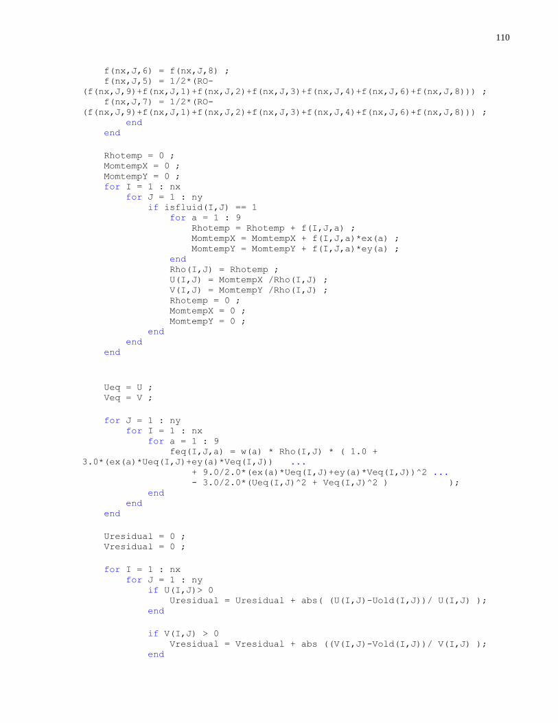
110
f(nx,J,6) = f(nx,J,8) ; f(nx,J,5) = 1/2*(RO-
(f(nx,J,9)+f(nx,J,1)+f(nx,J,2)+f(nx,J,3)+f(nx,J,4)+f(nx,J,6)+f(nx,J,8))) ; f(nx,J,7) = 1/2*(RO-
(f(nx,J,9)+f(nx,J,1)+f(nx,J,2)+f(nx,J,3)+f(nx,J,4)+f(nx,J,6)+f(nx,J,8))) ; end end
Rhotemp = 0 ; MomtempX = 0 ; MomtempY = 0 ; for I = 1 : nx for J = 1 : ny if isfluid(I,J) == 1 for a = 1 : 9 Rhotemp = Rhotemp + f(I,J,a) ; MomtempX = MomtempX + f(I,J,a)*ex(a) ; MomtempY = MomtempY + f(I,J,a)*ey(a) ; end Rho(I,J) = Rhotemp ; U(I,J) = MomtempX /Rho(I,J) ; V(I,J) = MomtempY /Rho(I,J) ; Rhotemp = 0 ; MomtempX = 0 ; MomtempY = 0 ; end end end
Ueq = U ; Veq = V ;
for J = 1 : ny for I = 1 : nx for a = 1 : 9 feq(I,J,a) = w(a) * Rho(I,J) * ( 1.0 +
3.0*(ex(a)*Ueq(I,J)+ey(a)*Veq(I,J)) ... + 9.0/2.0*(ex(a)*Ueq(I,J)+ey(a)*Veq(I,J))^2 ... - 3.0/2.0*(Ueq(I,J)^2 + Veq(I,J)^2 ) ); end end end
Uresidual = 0 ; Vresidual = 0 ;
for I = 1 : nx for J = 1 : ny if U(I,J)> 0 Uresidual = Uresidual + abs( (U(I,J)-Uold(I,J))/ U(I,J) ); end
if V(I,J) > 0 Vresidual = Vresidual + abs ((V(I,J)-Vold(I,J))/ V(I,J) ); end

111
end end Uold = U ; Vold = V ;
if mod(Loop_counter,100)==0 fprintf(' Iteration = %i, Uresidual = %f \n', Loop_counter, Uresidual) end
Loop_counter = Loop_counter + 1 ; end
fprintf('\n END!\n\n')
UP=zeros(nx,ny); VP=zeros(nx,ny);
UP=dx/dt*U; VP=dx/dt*V;
close figure set(gca,'FontSize',15) T=sqrt(UP.^2+VP.^2); surface(T) shading interp axis equal colorbar('FontSize',15) save (['Radius', num2str(10*runtime)])
IMFR = 0; for J = 1 : ny IMFR = IMFR + Rho(1,J)*U(1,J); end IMFR;
OMFR = 0; for J = 1 : ny OMFR = OMFR + Rho(nx,J)*U(nx,J); end OMFR;
abs(OMFR - IMFR)/IMFR
porosity = 0; for J = 1 : ny for I = 1 : nx porosity = porosity + isfluid(I,J); end end

112
porosity = porosity/(nx*ny)
dm=RhoP/RhoL*dx^3;
delta_pressure_L = (ROin - RO)/3;
delta_pressure_P = dm/(dx*dt^2)*delta_pressure_L;
Fluidnodes = 0; Usum = 0; for J = 1 : ny if isfluid(1,J) == 1 Usum = Usum + U(1,J); end end
for J = 1 : ny if isfluid(1,J) == 1 Fluidnodes = Fluidnodes + 1; end end
UinAVE = Usum/Fluidnodes; UinP = UinAVE *dx/dt; permeability1 = UinP*meu*nx*dx/delta_pressure_P
ReP = UinP*Radius*dx/Nu;

113
Checking for continuity (i.e. ��𝒊𝒏 ≈ ��𝒐𝒖𝒕):
The reader is advised to benchmark the following data with the above code prior to endeavoring
to use the code for further studies. Inlet and outlet mass flow rates were calculated for various
porosities to ensure that the mass was conserved (��𝑖𝑛 ≈ ��𝑜𝑢𝑡) in all of the cases:
Porosity \|��𝒊𝒏 − ��𝒐𝒖𝒕|/��𝒊𝒏
𝟎. 𝟗𝟖 1.1 × 10⁻⁶ 𝟎. 𝟗𝟔 1.0 × 10⁻⁶ 𝟎. 𝟗𝟑 4.1 × 10⁻⁷ 𝟎. 𝟗𝟎 2.4 × 10⁻⁶
𝟎. 𝟖𝟕 3.0 × 10⁻⁶
𝟎. 𝟖𝟓 3.2 × 10⁻⁶
𝟎. 𝟖𝟑 9.1 × 10⁻⁶
𝟎. 𝟕𝟖 2.7 × 10⁻⁵
𝟎. 𝟕𝟑 2.0 × 10⁻⁵
𝟎. 𝟔𝟕 1.4 × 10⁻⁴
𝟎. 𝟔𝟏 5.2 × 10⁻⁴
𝟎. 𝟓𝟒 4.3 × 10⁻⁴
𝟎. 𝟒𝟕 1.4 × 10⁻⁴
𝟎. 𝟑𝟗 3.3 × 10⁻⁵
𝟎. 𝟑𝟎 5.2 × 10⁻⁴