Numerical Analysis: Solving Nonlinear Equations …na191/wiki.files/NA191_lec...Numerical Analysis:...

Numerical Analysis:Solving Nonlinear Equations

(part I)

Computer Science, Ben-Gurion University

(slides based mostly on Prof. Ben-Shahar’s notes)

2018/2019, Fall Semester

BGU CS Solving Nonlinear Equations (ver. 1.00) AY 2018/2019, Fall Semester 1 / 29

1 Introduction

2 The Bisection Method


Introduction

Introduction

Our next topic for the several next lectures is solving nonlinear equations:

f : R→ R f(x) = 0 x =?

if x satisfies f(x) = 0, then it’s called a root of f .


Introduction

Introduction

The seemingly-more general cases of solving

f : R→ R f(x) = b x =?

can be rewritten in the original form above by defining a new function:

fnew : R→ R fnew : x 7→ f(x)− b fnew(x) = 0 x =?

Note:

fnew(x) = 0 ⇐⇒ f(x) = b


Introduction

Introduction

Likewise,

f : R→ R g : R→ R f(x) = g(x) x =?

can be handled via

fnew : R→ R fnew : x 7→ f(x)− g(x) fnew(x) = 0 x =?

Note:

fnew(x) = 0 ⇐⇒ f(x) = g(x)

Thus, WLOG, we will focus attention on solving f(x) = 0.


Introduction

The linear case

If f has the formf(x) = ax+ b

(that is, f is affine), where a and b are known real numbers, then we saythe equation is linear, and the solution to

f(x) = 0

is given (assuming a 6= 0), of course, by

x = − ba.


Introduction

Some Nonlinear Equations are Easy

Sometimes we know how solve nonlinear equations.

Examples:

x3 − 8 = 0⇒ x = 2 (one solution)

ax2 + bx+ c = 0⇒ x =−b±

√b2 − 4ac

2a(at most two solutions)

sin(x) = 0⇒ x = kπ, k ∈ Z (∞-many solutions)


Introduction

Nonlinear Equations

In general, however, if the equation is nonlinear we usually don’t knowhow to solve it analytically.


Introduction

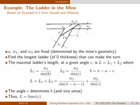
Example: The Ladder in the MineBased on Example 0.1 from Gerald and Wheatly

a, w1, and w2 are fixed (determined by the mine’s geometry).

Find the longest ladder (of 0 thickness) that can make the turn.

The maximal ladder’s length, at a given angle c, is L = L1 + L2 where

L1 =w1

sin(b)L2 =

w2

sin(c)b = π − a− c

L = L1 + L2 =w1

sin(π − a− c)+

w2

sin(c)

The angle c determines b (and vice versa).

Thus, L = func(c).


Introduction


L(c) =w1

sin(π − a− c)+

w2

sin(c)

The longest ladder that can pass is

mincL(c) .

Yes, minimum, not maximum. It’s the bottleneck that matters.


Introduction


mincL(c) = min

c

w1

sin(π − a− c)+

w2

sin(c)

From calculus, we know that c , argminc L(c) satisfies

dL

dc

∣∣∣∣c

= 0 .

Thus, we need to solve, for the unknown c, the following equation:

w1cos(π − a− c)sin2(π − a− c)

− w2cos(c)

sin2(c)= 0

Equivalently:

−w1cos(a+ c)

sin2(a+ c)− w2

cos(c)

sin2(c)= 0

How can we solve this?BGU CS Solving Nonlinear Equations (ver. 1.00) AY 2018/2019, Fall Semester 11 / 29

Introduction

Nonlinear Equations

Sometimes, in fact, even if a solution exists, an analytical form for itdoesn’t exist.

For example, the Abel-Ruffini theorem (also known as Abel’simpossibility theorem) states that this is the case for polynomials ofdegree higher than 4.

The theorem is named after Paolo Ruffini, who made an incomplete proof in1799,and Niels Henrik Abel, who provided a proof in 1824.


Introduction

Finding the Square Root of a Number

Another example we mentioned earlier: how can find the square root of anumber using only the 4 arithmetics operations (addition, subtraction,multiplication, and division) and the operation of comparison?

Example

x ∈ R≥0 x2 − 5 = 0 x =?


Introduction

Our discussion so far motivates the need for non-analytical methods,based on simple operations, as means to solving

f : R→ R f(x) = 0 x =?


Introduction

Trial and Error

One possible approach is trial and error.

Its disadvantage is that very little can be said, in general, about the itsexpected performance in terms of how fast it will find an approximatedsolution.


Introduction

Requirements from Numerical Methods

So we want methods that not only approximate a root but also lendthemselves to some useful analysis.

More generally (than the context of solving nonlinear equations), hereare our requirements from numerical methods:

SpeedReliabilityEase to useEasy to analysis


The Bisection Method


Sometimes, if a certain property (or certain properties) hold for f in acertain domain (e.g., some interval), it guarantees the existence of rootin that domain.

The Bisection method is an example for a method that exploits such arelation, together with iterations, to find the root of a function.




The Bisection method (AKA “interval halving” or “binary search”), is aparticular case of the so-called Bracketing methods.

Bracketing methods determine successively smaller intervals (brackets)that contain a root.



The bisection method utilizes the Intermediate Value Theorem.

Theorem (intermediate value)

Let f ∈ C([a, b]).If L ∈ R is a number between f(a) and f(b), that is,

min(f(a), f(b)) < L < max(f(a), f(b)) ,

then there exists c ∈ (a, b) such that f(c) = L.

C([a, b]) is the set of all continuous functions from [a, b] to R.BGU CS Solving Nonlinear Equations (ver. 1.00) AY 2018/2019, Fall Semester 19 / 29


A Useful Variant in Our Context

Particularly (taking L = 0):

f ∈ C([a, b]) and f(a) · f(b) < 0⇒ ∃c ∈ (a, b) such that f(c) = 0 .

In other words if f(a) and f(b) have opposite signs, then f must vanishat some c ∈ (a, b).



Definition (limit of a function at a point)

Let a function f be defined in an open interval containing x0, exceptpossibly at x0 itself. Then f has limit L at x = x0, denoted

limx→x0

f(x) = L ,

if ∀ε > 0 ∃δ such that

|x− x0| < δ ⇒ |f(x)− L| < ε .



Definition (continuity of a function at a point)

Let f be defined over the open interval (a, b) and let x0 ∈ (a, b). Thefunction f is said to be continuous at x = x0 if

limx→x0

f(x) = f(x0) .

Definition (continuity of a function over an open interval)

A function f is called called continuous over the open interval (a, b) if it iscontinuous at every x ∈ (a, b).

The definitions can be extended to the cases of [a, b), (a, b], or [a, b] usingone-sided limits at the relevant endpoints.



Notation

Cn([a, b]) , {f |f : [a, b]→ R, f and its first n derivatives are continuous}

Thus, C0([a, b]) is simply C([a, b]) (defined in a previous slide).

Example

f : x 7→ x4/3 is in C1([−1, 1]) but not in C2([−1, 1]), since

f ′ =4

3x1/3 f ′′ =

4

9x−2/3 =

4

9

1

x2/3

so f ′′ is discontinuous at x = 0.



The variant of the intermediate value theorem suggests the followingalgorithm.

Input: [a, b] (a bracket) such that f(a) · f(b) < 0; δ > 0 (a tolerance value)Output: z such that |z − z| < δ where z is a root of f (i.e., f(z) = 0)

1 repeat2 z ← 1

2(a+ b)

3 if f(a) · f(z) < 0 then4 b← z5 else6 a← z

7 until |b− a| < 2δ;8 z ← 1

2(a+ b)

Algorithm 1: The Bisection Method



Example

Figure: WikipediaBGU CS Solving Nonlinear Equations (ver. 1.00) AY 2018/2019, Fall Semester 25 / 29


Example (Multiple Roots)



Properties of the Bisection Method

Always works (assuming f is continuous): i.e., convergence to a trueroot is guaranteed:

limn→∞

z = z

Why? Since the approximation error after n iterations satisfies

E(n) <

∣∣∣∣b− a2n

∣∣∣∣(so E(n)→ 0)

The number of iterations required for a given approximation accuracy, δ,is known beforehand:

b− a2n≤ δ ⇒ n ≥ log2

(b− aδ

)BGU CS Solving Nonlinear Equations (ver. 1.00) AY 2018/2019, Fall Semester 27 / 29


Properties of the Bisection Method (Continued)

Convergence is relatively slow (i.e., a relative large number of iterationsis needed) – we will discuss this topic later on

E(n) might not be a monotonic decreasing function of n.

A big advantage: it is fairly easy to find a good initial guess.– as we will see, in other methods convergence is guaranteed to happenonly when the initial guess is close to the root. This requirement isunnecessary in the bisection method.

Multiple roots for which the function doesn’t change sign will be missed.



Version Log

24/10/2018, ver 1.00.


Numerical Analysis: Solving Nonlinear Equations …na191/wiki.files/NA191_lec...Numerical Analysis:...

Documents

Transcript of Numerical Analysis: Solving Nonlinear Equations …na191/wiki.files/NA191_lec...Numerical Analysis:...