
NUMERICAL ANALYSIS OF GAS FLOW WITHIN A MUNICIPAL SOLID WASTE
131
NUMERICAL ANALYSIS OF GAS FLOW WITHIN A MUNICIPAL SOLID WASTE LANDFILL A Thesis Submitted to the College of Graduate Studies and Research in Partial Fulfillment of the Requirements for the Degree of Master of Science in the Department of Civil Engineering University of Saskatchewan Saskatoon by Natalya Viktorovna Usova © Copyright Natalya V. Usova, July 2012. All rights reserved.
Transcript of NUMERICAL ANALYSIS OF GAS FLOW WITHIN A MUNICIPAL SOLID WASTE

NUMERICAL ANALYSIS OF GAS FLOW WITHIN A MUNICIPAL
SOLID WASTE LANDFILL
A Thesis
Submitted to the College of Graduate Studies and Research
in Partial Fulfillment of the Requirements
for the Degree of Master of Science
in the Department of Civil Engineering
University of Saskatchewan
Saskatoon
by
Natalya Viktorovna Usova
copy Copyright Natalya V Usova July 2012 All rights reserved
i
PERMISSION TO USE
The author has agreed that the library University of Saskatchewan may make this
thesis freely available for inspection Moreover the author has agreed that permission
for copying of this thesis in any manner in whole or in part for scholarly purposes may
be granted by the professors who supervised the thesis work recorded herein or in their
absence by the Head of the Department or the Dean of the College in which the thesis
work was done It is understood that due recognition will be given to the author of this
thesis and to the University of Saskatchewan in any use of the material in this thesis
Copying or publication or any other use of the thesis for financial gain without approval
by the University of Saskatchewan and the authorrsquos written permission is prohibited
Requests for permission to copy or to make any other use of material in this thesis in
whole or part should be addressed to
Head of the Department of Civil and Geological Engineering
University of Saskatchewan
Engineering Building
57 Campus Drive
Saskatoon Saskatchewan
Canada S7N 5A9
ii
ABSTRACT
Numerical analysis and modelling of gas flow within a municipal solid waste (MSW)
landfill has the potential to significantly enhance the efficiency of design and
performance of operation for landfill gas (LFG) extraction and utilization projects Over
recent decades several numerical models and software packages have been developed
and used to describe the movement and distribution of fluids in landfills However for
the most part these models have failed to gain widespread use in the industry because
of a number of limitations Available simple models implement a simple theoretical
basis in the numerical solution for example various approaches that treat the landfilled
waste fill purely as a porous medium with the conservation of mass inherently assumed
and the ongoing gas generation within the landfill thus ignored Alternatively
researchers have developed some highly complex models whose use is rendered
difficult as a result of the uncertainty associated with the large number of required
inputs
Ultimately more efficient design and operation of well-fields for LFG extraction will
provide a benefit in the cost of construction and efficiency of operation as well as with a
reduced potential of underground fire resulting from over-pumping or localized
excessive wellhead vacuum Thus the development of tools for improved
understanding and prediction of the gas flows and pressure distribution within MSW
will potentially enhance operation of LFG extraction systems at existing landfills as
well as the design for new LFG projects In the simplest terms a more accurate estimate
of the relationship between flow rates and wellhead vacuum will allow for improved
analysis of the network of LFG extraction wells header pipes and valves and blowers
The research described in this thesis was intended to evaluate the error introduced into
estimates of the intrinsic permeability of waste from LFG pumping tests if the ongoing
gas generation within the landfilled MSW is ignored when the pumping tests are
evaluated to yield estimates of the permeability The City of Saskatoonrsquos Spadina
Landfill Site was chosen as the research site The landfill contains over six million
tonnes of waste of age ranging from days and weeks old to almost 60 years and which
iii
continue to generate significant landfill gas It was determined that during the pumping
tests the estimated volume of gas generated within the radius of influence of each well
during the time of pumping ranged from 20 to 97 of the total volume of the gas
actually pumped during the time of the pumping depending on the well and the flow
rate in question Fleming (2009) reported that the landfill is estimated to generate about
250[m3hour] of landfill gas containing up to 60 of methane
Two different approaches were used to simulate gas flow in the unsaturated waste fill
The first modelling tool was the GeoStudio 2007 software suite The second approach
used a very simple 1-dimensional axisymmetric finite difference (1-D FD) solution to
estimate the radial distribution of pressures within the waste associated with gas flow
toward an applied wellhead vacuum under conditions where the waste fill is estimated
to generate landfill gas at a constant rate per unit volume This 1-D FD solution was
used to compare the flow rate and pressure distribution in the waste with that predicted
using widely-available geotechnical software for 2-dimensional axisymmetric flow in
an unsaturated porous medium It is proposed that the correction charts so developed
may represent a first step toward a reliable method that would enable such widely used
software to be used with a correction factor to enable improved simulations of flow and
pressure within the system
The results from both approaches support the previously reported intrinsic permeability
values determined for the Spadina Landfill The 1-D FD solution results show that there
is some effect of the gas generation on the best-fit estimates of the value of intrinsic
permeability In addition the 1-D FD solution shows better fit to the field data (when
the gas generation is taken into account) compared with simulations carried out using
AIRW (GeoStudio 2007)
Nevertheless the AIRW computer package was found to be simple powerful and
intuitive for simulating two-phase flow toward LFG extraction wells The addition of
an option to include a gas generation term in the commercial software package would
enable more accurate results for evaluation of flow of landfill gas however as a first
step in this direction charts of correction factors are proposed
iv
ACKNOWLEDGEMENTS
I would like to express my appreciation and respect to my supervisor Prof Ian
Fleming for his invaluable support guidance and advice His critical appraisal and
recommendations have been priceless at every stage of this research and the evolution
of the writing of this thesis
I would like to extend my acknowledgement to my committee chair Dr Moh Boulfiza
and my advisory committee members Dr Jit Sharma Dr Grant Ferguson and Dr
Chris Hawkes for their valuable suggestions and feedback
I take this opportunity to thank graduate students colleagues and staff at the
Department of Civil and Geological Engineering for making my stay at the University
of Saskatchewan one of the most memorable moments of my life
Furthermore I would like to thank NSERC the City of Saskatoon and SALT Canada
Inc for providing the financial support for this research work
v
DEDICATIONS
The thesis is dedicated to my husband for his priceless motivation encouragement and
guidance and to my daughter two sisters father and grandmother for their valuable
support
vi
TABLE OF CONTENTS
PERMISSION TO USE I
ABSTRACT II
ACKNOWLEDGEMENTS IV
DEDICATIONS V
TABLE OF CONTENTS VI
LIST OF TABLES VIII
LIST OF FIGURES IX
LIST OF VARIABLES XII
CHAPTER 1 INTRODUCTION 1
11 Background 1
12 Research objective and scope 3
13 Research Methodology 5
14 Thesis Outline 6
CHAPTER 2 LITERATURE REVIEW AND BACKGROUND 8
21 Introduction 8
22 Multiphase Flow in Porous Media 8
221 Consideration Regarding Conservation of Mass 17
222 The Specifics of Two-Phase Flow in MSW 18
23 Available Software Packages for Analysis of Landfill Gas Flow in MSW 24
CHAPTER 3 METHODOLOGY 30
31 Introduction 30
32 The City of Saskatoon Spadina Landfill Site 31
33 AIRW Models 32
331 Geometry and Boundary Conditions 32
332 Material Properties 35
333 Model Validation 37
vii
334 Parametric Study of the Effects of Anisotropy and Partial Penetration 40
335 Non-Convergence and Initial Simulations 46
34 1-D finite difference solution to gas generation and flow in a homogeneous porous
medium 48
341 Mathematical Approach and Model Geometry with Its Boundary Conditions 48
342 Model Validation 53
343 Parametric Study of the Effect of Gas Generation 57
CHAPTER 4 PRESENTATION OF RESULTS ANALYSIS AND DISCUSSION 59
41 Introduction 59
42 AIRW Parametric Study of the Effects of Anisotropy and Partial Penetration 60
43 Comparing the AIRW modes and 1-D FD solution (Rg=0) results 68
44 The 1-D FD Solution 71
441 Initial Results 71
442 Parametric Study of the Gas Generation Effect 71
45 Worked example 80
CHAPTER 5 SUMMARY CONCLUSIONS AND RECOMMENDATIONS 84
51 Introduction 84
52 Summary and Conclusions 85
53 Significance of the findings 87
54 Need for further research 88
LIST OF REFERENCES 90
APPENDICES 97
APPENDIX A TEST-WELLS GEOMETRY AND LANDFILLED DATA 98
APPENDIX B MODEL INPUTS FOR BOTH AIRW AND 1-D FD SOLUTION 102
APPENDIX C AIRW MODEL RESULTS 103
APPENDIX D 1-D FD SOLUTION RESULTS 108
APPENDIX E STATISTICAL ANALYSIS OF BEST-FIT 114
viii
LIST OF TABLES
Table 2 1 Range of waste hydraulic conductivity in depth profile 22
Table 2 2 Anisotropy of hydraulic conductivity obtained by laboratory testing waste23
Table 2 3 Intrinsic permeability of MSW in radial direction and flow rate due to depth
change (after Jain et al 2005) 24
Table 3 1 Model geometry used to evaluate PP and anisotropy 43
Table 3 2 Gas flow rate and generated gas flow within volume of influence 52
Table 3 3 Input parameters and boundary conditions for the 1-D FD solution (GW01-
04) 54
Table A 1 Test-wells geometry as were constructed in the field 98
Table A 2 Measured field data during the short-term pumping tests at GW01-04
GW02-04 GW04-07 and GW10-07 99
Table A 3 Radius of influence (ROI) for test-wells (after Fleming 2009) 101
Table B 1 Time and radius increment used in the 1-D FD and step-by-step time length
used in 1-D FD AIRW 102
Table C 1 AIRW input intrinsic permeability values within the parametric study
analysis 103
Table D 1 The geometric mean of air and intrinsic permeability results with its gas
generation rate obtained using the 1-D FD analysis 111
Table D 2 The 1-D FD solution results within the parametric studies and the AIRW
input intrinsic permeability values 112
Table D 3 The relationship between the intrinsic permeability correction factor due to
gas generation and the gas ratio 113
ix
LIST OF FIGURES
Fig 2 1 Fitting a gap-graded soil with the unimodel and bimodel equations 10
Fig 2 2 Typical relative permeability curves (after Bear 1972) 13
Fig 2 3 Schematic for the partial differential equation (after Barbour 2010) 14
Fig 2 4 Factors affecting landfill dynamics (after Kindlein et al 2006) 19
Fig 2 5 Theoretical curves of volumetric water content against applied stress in low
accumulation conditions (after Hudson et al 2004) 20
Fig 2 6 Unit weight profiles for conventional municipal solid-waste landfills and the
effect of confining stress is represented by depth (after Zekkos et al 2006) 21
Fig 3 1 Test well and monitoring probe locations at the Spadina Landfill Site (after
Fleming 2009) 31
Fig 3 2 Schema of an AIRW model geometry 32
Fig 3 3 Boundary conditions for an AIRW model 33
Fig 3 4 Gas pressure (a) Best-fit gas pressure P(t) for the measured gas pressure data
during the short-term field test at GW01-04 GW02-04 and GW10-07 which were used
as a boundary condition at a wellbore area in the models (b) (c) and (d) goodness of
fitting respectively for GW01-04 GW02-04 and GW10-07 34
Fig 3 5 Relative permeability curves used in AIRW 36
Fig 3 6 Moisture retention curves used in AIRW and Kazimoglu et al 2006 37
Fig 3 7 AIRW model outputs for two different estimation methods of the input
hydraulic conductivity function 39
Fig 3 8 Parametric Study for GW01-04 and GW02-04 AIRW models 41
Fig 3 9 Parametric Study for GW10-07 AIRW model 42
Fig 3 10 Changing the total AIRW models depth (GW01-04 GW02-04 and GW10-
07) for investigating PP and anisotropy 44
Fig 3 11 Monitoring pressure response measured in the field and AIRW output
pressure profile at different depths for (a) GP 01-04 and (b) GP 02-04 45
x
Fig 3 12 Convergence in result simulations the red colour is shown for non-
convergence and the green colour is for convergence 47
Fig 3 13 Typical geometry and its initial and boundary conditions for a 1-D FD
solution 51
Fig 3 14 Log(ki) versus radius of influence relationship for GW01-04 test-well 53
Fig 3 15 The 1-D FD solution (a) Scenario I boundary condition as the defined gas
flow rate at GW-01-04 and the 1-D FD solution (b) Scenario II boundary condition as
the measured gas pressure at the same well (GW-01-04) and the 1-D FD solution
output 55
Fig 3 16 Measured gas pressure during the short-term field test at all four test wells
and SEEPW and 1-D FD solution outputs based on the same best-fit values of intrinsic
permeability respectively 56
Fig 3 17 Parametric Study for 1-D FD solution for GW01-04 and GW02-04 wells 57
Fig 3 18 Parametric Study for 1-D FD solution for GW04-07 and GW10-07 wells 57
Fig 4 1 Three models with four simulated gas flow outputs made in the AIRW for the
initial 36[m] case (a) GW01-04 (b) GW02-04 and (c) GW10-07 61
Fig 4 2 Gas flow rate measured during the short-term field test at GW01-04 and
AIRW results based on the best-fit values of ki[m2] with different PP ratio and
anisotropy to be equal one in GW01-04 AIRW model 63
Fig 4 3 Intrinsic permeability values used for the best-fit AIRW modelsrsquo outputs 65
Fig 4 4 The intrinsic permeability ratio verses the partial penetration ratio for the
AIRW models for (a) GW01-04 (b) GW02-04 and (c) GW10-07 66
Fig 4 5 Parametric study results for the best-intrinsic permeability values (a) the
AIRW intrinsic permeability inputs compare to the previously defined values in the
field (after Schmidt 2010) and (b) the AIRW intrinsic permeability inputs 67
Fig 4 6 Defined intrinsic permeability values based on the obtained results from
AIRW and 1-D FD solution (a) 1-D FD solution and AIRW results from parametric
studies (b) AIRW and 1-D FD comparable results 69
Fig 4 7 Typical difference in relative permeability curves of gas in AIRW and 1-D
FD solutions 70
Fig 4 8 Effect of assumed gas generation on predicted wellbore vacuum under
pumping rates and air permeability value best-fit from zero-gas generation scenario for
following test-wells (a) GW01-04 (b) GW02-04 (c) GW04-07 and (d) GW10-07 72
xi
Fig 4 9 The 1-D FD solutions for both settings where the total gas generation is taken
in account and where it is ignored with their boundary condition as the defined gas flow
rate at the wellbore area and the 1-D FD solution outputs based on the best-fit value kir
for each of the four test-wells (a) GW01-04 (b) GW02-04 (c) GW04-07 (d) GW10-
07 74
Fig 4 10 Statistics for best-fit data using 1-D FD defined for GW01-04 (a) 1st
drawdown step and (b) 2nd
step 76
Fig 4 11 The geometric mean of the air permeability values obtained through 1-D FD
solution within the parametric studies 77
Fig 4 12 1-D FD solution outputs Logarithm to the base ten of the intrinsic
permeability verses the total gas generation rate 78
Fig 4 13 The functions of the intrinsic permeability correction factor due to gas
generation and the gas ratio based on the data sets from the following test-wells
GW01-04 GW02-04 GW04-07 and GW10-07 80
Fig 4 14 Use of correction φkR to estimate the gas generation rate using pumping test
data 82
Fig C 1 Several simulated gas flow outputs that show the partial penetration and
anisotropy effects in GW01-04 AIRW model 104
Fig C 2 Several simulated gas flow outputs that show the partial penetration and
anisotropy effects in GW02-04 AIRW model 105
Fig C 3 Several simulated gas flow outputs that show the anisotropy effects in GW10-
07 AIRW model 106
Fig C 4 Gas flow rate during the short-term field test at GW-01-04 vs AIRW output
based on a best-fit value kir=27310-13
[m2] (initial case kxky=1 and LSDT0) 107
Fig D 1 SEEPW simulation results respectively for each test-well 108
Fig D 2 Measured gas pressure during the short-term field test at all four test wells
and SEEPW and 1-D FD solution outputs based on the same best-fit values of air
permeability respectively 110
Fig D 3 The relationship between the intrinsic permeability correction factor due to
gas generation and the gas ratio based on the data from the following test-wells GW-
01-04 GW-02-04 GW-04-07 GW-10-07 113
xii
LIST OF VARIABLES
anm = curve fitting parameters (eq[33])
A = surface area of the screened portion of a well [m2]
d = representative length dimension of the porous matrix [m]
= gradient of hydraulic (total) head [mm]
= gas pressure gradient [Pam]
DT = total depth of the mode [m]
Dwaste = entire depth of waste [m]
e = natural number 271828
= methane fraction
g = gravitational acceleration [ms2]
hpw = hydraulic pressure head [m]
i = interval between the range of j to N
j = least negative pore-water pressure to be described by the final function
Ii = rate at which mass of the i-species is produced per unit volume of the system by the
chemical reaction [kg(m3s)]
Ik = intrinsic permeability ratio [dimensionless]
Kw = hydraulic conductivity [ms]
Kw = calculated hydraulic conductivity for a specified water content or negative pore-
water pressure [ms]
Ks = saturated hydraulic conductivity [ms]
Ksm = measured saturated conductivity [ms]
Kx and Kz = horizontal and vertical hydraulic conductivity respectively [ms]
ki = intrinsic permeability [m2]
kir = intrinsic permeability in radial direction [m2]
kiz = intrinsic permeability in vertical direction [m2]
= best-fit value of intrinsic permeability determined using the AIRW model
assuming a geometry that is closest to a fully-penetrated well screen within the
constants of convergence described above [m2]
xiii
= best-fit value of intrinsic permeability using the AIRW model with the actual
partially-penetrating geometry of each well as actually constructed [m2]
= intrinsic permeability determined using the 1-D FD solution with the total gas
generation rate included (Rggt0) [m2]
= intrinsic permeability determined using the 1-D FD solution but where the total
gas generation rate was ignored (Rg=0) [m2]
kra = relative permeability of air [dimensionless]
krnw = relative permeability of non-wetting fluid[dimensionless]
krw = relative permeability of water (or wetting fluid)[dimensionless]
ka = air effective permeability [m2] (= kramiddotki )
kw = water effective permeability [m2] (= krwmiddotki)
kxkz = anisotropy ratio [dimensionless]
LDS = depth to the screen [m]
LS = screen length [m]
LSB = distance from the screen bottom to the model bottom [m]
LSDT = partial penetration ratio [dimensionless]
MW = molecular weight of gas [kgmole]
N = vector norm i is a counter and n is the total number of nodes (eq [31])
N = maximum negative pore-water pressure to be described by the final function (eq
[32])
microg = gas viscosity [kg(ms)]
μw = absolute (dynamic) viscosity of water [N sm2]
P = gas pressure [Pa]
Patm = ambient gas pressure [Pa]
= gas density [kgm3]
= density of the i-species [kgm3]
ρw = density of water [kgm3]
= apparent density of waste [Mgm
3]
Qg = gas flow rate (Darcyrsquos Law) [m3s]
θg = volumetric gas content equal the product of the gas ndashphase saturation and the
porosity [m3m
3]
θw = volumetric moisture content [m3m
3]
xiv
qi = specific discharge of the i-species [ms]
qg = specific discharge of gas (Darcyrsquos Law) [ms]
qw = specific discharge of water [ms]
r = distance from the pumping well [m]
rp = Pearsonrsquos correlation coefficient
rw = well radius [m]
R = ideal gas law constant (taken as 8314 [Pam3(Kmole)])
= methane generation rate [m
3Mgyear]
R2 = coefficient of determination
Re = Reynolds number [dimensionless]
Reg = Reynolds number for gas flow [dimensionless]
Rg = total gas generation rate [kg(m3s)]
= total gas generation rate [m
3m
3hour]
RM = radius of the model [m]
S = saturation which is defined as the ratio of the volume of wetting fluid to the volume
of interconnected pore space in bulk element of the medium [dimensionless]
(or θe) = effective saturation [dimensionless]
Snw = non-wetting fluid saturation (ie Snw0 is residential)
Sr = residual saturation [dimensionless]
Sxx and Syy = statistics that used to measure variability in variable ldquoxrdquo and ldquoyrdquo
correspondently [dimensionless]
Sxy = statistic that used to measure correlation [dimensionless]
Sw = wetting fluid saturation (ie Sw0 is irreducible)
t = time [s]
T = absolute temperature [K]
Ua and Uw = correspondently the air and the water pressures
(Ua-Uw)i = individual nodal matric pressure
Vscreen = screen volume [m3]
Vwaste = waste volume [m3]
x = distance from the pumping well [m]
y = a dummy variable of integration representing the logarithm of negative pore-water
pressure z is the thickness [m]
υg = kinematic viscosity of the gas [m2s]
xv
= intrinsic permeability correction factor due to gas generation [dimensionless]
Θs = volumetric water content [m3m
3]
Θrsquo = first derivative of the equation
Ψ = required suction range
Ψ = suction corresponding to the jth
interval
λ = Brooks-Corey pore-size distribution index [dimensionless]
= gas ratio [1m3]
poundRg = volume of gas generated per unit time [m3hour]
1
CHAPTER 1
INTRODUCTION
11 Background
During recent decades in most countries landfills have been constructed to separate
waste deposits from the nearby environment and have represented the primary means of
solid waste disposal In fact the problem of contamination from landfills has become an
important international challenge (Amro 2004) During operation and subsequently
landfilled waste is exposed to various physical and biochemical effects As a result
various processes occur including generation of heat and landfill gas flow of leachate
and gas and mechanical deformation and settlement (Kindlein et al 2006 Powrie et al
2008) The stabilization of municipal solid waste (MSW) landfills can be viewed as a
two-phase process an early aerobic decomposition phase followed by an anaerobic
phase The aerobic phase is relatively short inasmuch as biodegradable organic
materials react rapidly with oxygen to form carbon dioxide water and microbial
biomass Thereafter landfill gas is generated consisting of a mixture of gases which are
the end products of biodegradation of organic materials in an anaerobic environment
(El-Fadel et al 1997a)
Increasing awareness of and concern regarding the potential environmental impact of
municipal waste landfills have combined with evolving technology for landfill gas
capture and utilization MSW landfills have thus increasingly become a focus of
research for both economic and environmental reasons Existing and proposed landfills
must meet environmental regulations which typically specify minimum standards for
protecting the environment and thus impose potential economic costs for example by
requiring collection and flaring of landfill gas (LFG)
2
The minimization of environmental impact has been significantly reinforced by
research In many cases continuing improvements to the efficiency performance and
economics of current or prospective LFG projects usually require expensive and time
consuming testing and evaluation and the resulting well-field designs may not in any
event attain the best possible efficiency and optimization
Numerical analysis and modelling can thus play an important role in this rapidly
developing field In general for many projects including design of landfill barrier
systems numerical analysis and modelling have become an inalienable part of
engineering because of the ability to be used in at least three generic categories such as
interpretation design and prediction of different scenarios (Barbour and Krahn 2004)
Modelling of landfill gas generation and extraction particularly relating to well-field
design and optimization is relatively less advanced
The fundamental theory of fluid flow in porous media was developed for groundwater
oil and gas and related flow phenomena Jain et al (2005) White et al (2004)
Kindlein et al (2006) and others commonly refer to the governing equations for
multiphase flow and transport in porous media the models that were earlier presented
by various authors including Bear (1972)
Published papers related to multiphase flow in waste fill in most cases attempt to apply
established models developed for groundwater flow or related phenomena to the
particularly conditions found in a landfill As a result applications of such modified
models may be quite limited in terms of the range of applicability as a result of the
restrictive assumptions and limited cases of applications For example available
software packages and numerical models treat the landfilled waste as a porous medium
with the inherent assumption of conservation of mass thereby by necessity ignoring in-
situ LFG generation Also depending on the approach a landfill investigation can
represent different space and time scales For example White et al (2004) described the
biochemical landfill degradation processes of solid waste using a numerical model of
various coupled processes where they make several assumptions for instance that any
gas with pressure in excess of the local pore-pressure is vented immediately It is
3
evident that this assumption can never be completely realized as for the real spatial
dimensions of the landfill some finite duration of time would be required
To improve the understanding of gas flow processes in unsaturated landfilled MSW
this research was intended to assess the effect of ignoring gas generation in estimating
the intrinsic permeability of waste from LFG pumping test data Efficient well-field
design requires accurate knowledge of the flowvacuum relationship for the wells and it
will be demonstrated that the relationship between flow and wellhead vacuum is
affected to a significant degree by the in-situ generation of gas within the waste fill In
addition a potential safety consideration reflects the fact that waste degradation goes
along with high subsurface temperature Overpumping of wells as a result of
underestimating the relationship between gas flow rate and pumping pressure (vacuum)
may thus increase the risk of underground fire Therefore the ability to accurately
define the material properties of a landfill can be considered important from the
perspective of health and safety and more accurate estimates of permeability and
relationship between flow rate and wellhead vacuum will provide a benefit in the cost of
construction and efficiency of landfillrsquos operation
12 Research objective and scope
This research is carried out using pumping test data that have been previously collected
by Stevens (2012) from the City of Saskatoonrsquos Spadina Landfill Site and the authorrsquos
work is therefore strictly confined to the analysis of combined LFG generation and flow
using these test data This landfill site has operated since 1955 and by 2007 stored over
six million tonnes of waste The ongoing degradation of MSW generates landfill gas at
a relatively moderate rate Fleming (2009) reported that the demonstration well-field
(10-test wells) was capable of producing on average about 250[m3hour] of landfill gas
where the methane fraction ranged from 50 to 60 The rate of gas generation at
Spadina Landfill Site was estimated to be approximately equal to 4 m3 of methane per
Mg of waste in-situ per year Moreover if a modest increase in the in-situ moisture
content may be achieved the stable methane generation rate could reach 10 to
20[m3Mgyear] (Fleming 2009) During the pumping tests the estimated volume of gas
4
generated within radius of influence of each well during the pumping time ranged from
20 to 97 of the total volume of gas that was actually pumped during the time of
pumping depending on the well and the flow rate Thus the purpose of this work is to
investigate the effect of ignoring or including the gas generation rate when carrying out
analyses of the data collected from LFG pumping tests and to determine the magnitude
of this effect in estimating the (intrinsic) permeability of the waste mass using
numerical analysis and modeling
The general objective of this research project is to define an appropriate conceptual
basis and a numerical model for combined gas generation and flow in MSW based on
the principle of intrinsic permeability and to determine the effect of the gas generation
rate on the permeability estimates determined from pressureflow data collected from
LFG pumping tests in MSW
The specific objectives are as listed below
To conduct a literature review of existing numerical techniques for unsaturated
flow in MSW landfills
To evaluate the intrinsic permeability of MSW using test data collected from the
City of Saskatoonrsquos Spadina Landfill Site
To develop two approaches for a gas flow model for MSW
o The first model tool was the commercial software package called AIRW
(GeoStudio 2010) which was used to evaluate the conceptual model for
gas flow to extraction wells within unsaturated MSW
o The second approach used a simple 1-dimensional axisymmetric finite
difference solution to estimate the radial distribution of pressures when
the effect of gas generation within the waste mass is included
To determine if gas generation occurring in the landfill may be ignored in the
evaluation of the (intrinsic) permeability of the landfilled waste
To propose correction charts that incorporate gas generation term so the results
from the widely used software could be improved within a correction factor and
5
To offer recommendation for future research
The research was restricted to analysis based on the data previously collected by
Stevens (2012) and thus the data collection instruments and test methods used to
gather the data are not considered in this research
13 Research Methodology
No previous research has been found that addresses this issue of the effect of the gas
generation rate on the estimated permeability of MSW The research program for this
thesis followed a standard modelling methodology A simple version of the scientific
methodology covers four steps which are to observe to measure to explain and to
verify (Barbour and Krahn 2004) The methodology for each approach was followed
during the four main steps in this thesis
Step 1 Observe ndash develop the conceptual model The three key processes were
included such as defining the purpose of the model gathering existing
information and developing a conceptual model
Step 2 Measure ndash define the theoretical model Discussion of the important
processes occurring in association with the most relevant equations and theories
Statement of the essential assumptions and approximations used in definitions
including available data sets of all known information
Step 3 Explain ndash develop and verify the numerical model Define the model
geometry and set boundary conditions and material properties The obtained
solution was compared with an alternative solution and published field studies to
establish its accuracy Possible sources of error were determined and the
limitation of the solution obtained
Step 4 Verify ndash interpret calibrate validate After the solution was obtained
the results were interpreted within the context provided by the observed physical
reality and calibrated and validated to capture defects in the solution if they
existed The range of reasonable and acceptable responses to the solutions was
defined A sensitivity analysis was carried out through a selected range of
6
relevant parameters The sensitivity analysis involved a series of simulations in
which only one parameter was varied at a time and then reviewed for defining
what was the effect of these variations against the key performance Confirm the
model by applying the calibrated model to the new set of responses The results
of both approaches were recorded compared and the work was submitted for
review
14 Thesis Outline
This research study delivers the background which is needed for the development of a
numerical analysis of gas generation and flow within a MSW landfill The thesis
includes five chapters and four appendices
The first chapter introduces the problem lists the objectives and the scope and briefly
describes the research methodology
Chapter 2 provides the literature review which includes the summary of the related
research conducted previously and describes the physical problems
Chapter 3 presents a description of the investigated site together with the methodology
for both modelling approaches The first approach is the transient axisymmetric two-
phase saturatedunsaturated flow model built using the widely-available commercial
software GeoStudio 2007 (AIRW) The second approach is a simple one-dimension
finite difference numerical solution for combined gas generation and flow The detailed
parametric study for both approaches is shown in Chapter 3
Chapter 4 shows what have been learned through the presentation analysis and
discussion of the results obtained from both modelling approaches
Chapter 5 summarizes the work described in this thesis together with one worked
example of the proposed methodology The need for the further research is outlined
there as well
7
The appendices present the outputs from both approaches in graphical orand in tabular
forms as well as additional information that helps to improve understanding of the
research described in this thesis The field data and properties together with its test-well
geometry conducted previously (Stevens 2012 and Fleming 2009) are provided in
Appendix A The modelsrsquo geometry and their boundary conditions for both approaches
can be found in Appendix B The outputs of the AIRW modelsrsquo simulations conducted
through the parametric study are shown in Appendix C The outputs of the 1-D FD
solution conducted through the parametric study are shown in Appendix D Appendix D
provides extra information for the correction factors and charts for intrinsic
permeability which have been newly defined through this research
8
CHAPTER 2
LITERATURE REVIEW AND BACKGROUND
21 Introduction
Gas flow within a MSW landfill is governed by the well-established principles of flow
in porous media and in this chapter the background is presented for the development of
a rigorous analysis of the problem This chapter is divided into three sections The first
section provides the background of the physical problem under consideration and a
review of related previous research The next section describes the material-specific
properties of MSW along with factors that affect the gas flow in MSW based on earlier
research The last section presents a discussion regarding available software packages
that may be used to investigate a one or two-phase flow of fluids in a MSW landfill
22 Multiphase Flow in Porous Media
The following section describes the theoretical background of unsaturated porous
medium theory required to develop the equations for the numerical analysis
The complexity of two-phase flow in porous media is discussed by Knudsen and
Hansen (2002) and by Bravo et al (2007) who highlight problems such as the
difference between unsteady and transient response the relations of properties at
different length scales and the existence of a variety of flow patterns It is well
established that when two or more fluids occur in porous media two types of flow are
possible to observe miscible displacement and immiscible displacement (Bear 1972) In
the case of simultaneous flow of two-phases (liquid and gas) immiscible displacement
flow occurs under conditions such that the free interfacial energy is non-zero and a
distinct fluid-fluid interface separates the fluid within each pore (Bear 1972) The
research carried out for this work covered unsaturated flow which is a special case of
9
the flow of two immiscible fluids Unsaturated (air-water) flow represents the flow of
water and water vapour through a soil where the void space is partly occupied by air
(ie the flow of water that has the degree of saturation less than 100 with stagnant air
that is partially occupied the void space not filled with water) (Bear 1972)
Experimental results have demonstrated that when two-phase flow of immiscible fluids
occurs simultaneously through a porous medium each of them creates its own tortuous
flow paths forming stable channels (Bear 1972) Therefore in many cases it is assumed
that a unique set of channels acts in conformity with a given degree of saturation (Bear
1972 and Bravo et al 2007) Relative permeability soil structure and stratification
depth to the ground water and moisture content are the major parameters that are used
to evaluate permeability of porous media
A fundamental property of an unsaturated porous media is reflected by the moisture
retention curve which describes the relationship between suction (or the negative pore-
water pressure) and moisture content (Bear 1972 Fredlund and Rahardjo 1993
McDougall et al 2004) When the gravimetric moisture retention curve is determined
through the pore-size distribution it is assumed that the moisture lost as a result of an
increase in suction corresponds to the volume of pores drained (Simms and Yanful
2004) In an unsaturated soil the permeability is significantly affected by combined
changes in the soil moisture content (or saturation degree) and the soil void ratio
(Fredlund and Rahardjo 1993) Both parameters may be readily incorporated if the
saturation condition is expressed in terms of an effective degree of saturation The
effective degree of saturation can be expressed in the following form as (Corey 1954
1956)
[2 1]
where is the effective saturation [dimensionless] S is the saturation which is defined
as the ratio of the volume of wetting fluid to the volume of interconnected pore space in
bulk element of the medium [dimensionless] 1 is the volumetric moisture content at
saturation 100 and Sr is the residual saturation [dimensionless]
10
The moisture retention curve is commonly determined experimentally however the
shape of moisture retention curve can be also estimated predominantly by the grain-size
distribution data and secondarily by the density of the soil through a mathematical
approach (Fredlund et al 2002) Fredlund et al (2000) proposed a unimodal equation
for uniform or well graded soils and a bimodal equation for gap-graded soils essentially
enabling fitting to any grain-size distribution data set (Fig 21)
Fig 2 1 Fitting a gap-graded soil with the unimodel and bimodel equations
(after Fredlund et al 2000)
Later Fredlund et al (2002) proposed a method to estimate a moisture retention curve
from the grain-size distribution calculated using this method They reported good fits
for the estimated moisture retention curves for sand and silt and reasonable results for
clay silt and loam Huang et al (2010) compared the estimated and measured grain-
size distribution curves presented by Fredlund et al (2000) with their samples and
found that results differed with a lower root mean square error of 0869 The authorsrsquo
research was based on a data set of 258 measured grain-size distribution and moisture
retention curves (Huang et al 2010) Additional investigation is still required in testing
11
the algorithms on finer soils and on soil with more complex fabrics or indeed non-
conventional ldquosoil-like materialsrdquo such as MSW
When the moisture retention curve for two-phase immiscible flow is analyzed it is
necessary to consider the more complicated porosity model In porous media there can
be several conceptual models used to idealize the pore size distribution such as single-
dual- and multiple-porosity Since this research focused on two-phase flow in a MSW
landfill the dual-porosity becomes a point of interests
Fluid flow in MSW has been shown to exhibit behaviour characteristic of a dual
porosity model with large easily-drained pores and a matrix of smaller pores
(Kazimoglu et al 2006 White et al 2011 and Fleming 2011) Thus it is possible that a
gap-graded particle size approach might be suitable for estimating or predicting the
moisture retention properties of landfilled MSW
Dual-porosity models differ from single-porosity models by the presence of an
additional transfer function (Tseng et al 1995) Dual-porosity models have been
extended and used since 1960 when Barenblatt and Zheltov (1960) and Barenblatt et al
(1960) introduced a conceptual double-continua approach for water flow in fissured
groundwater systems In general the dual-porosity model appears to approximate the
physical unit of a structured porous medium with two distinct but at the same time with
interacting subunits that represent macro-pores and porous-blocks inherent in the field
soil or rock formations Because of its complexity existing formulations of the dual
porosity model have been developed with many simplifications and idealized
assumptions Moreover in case of the dual-porosity for the two-phase MSW landfill
flow there are further complications that needed to be better researched (ie it was not
found how the ignorance of a dual-porosity might affect the results)
The fundamental parameter which affects flow (ie single-phase and two-phase) in
porous media is the intrinsic permeability First of all it is obvious that the ability of a
soil to transmit gas is reduced by the presence of soil liquid which blocks the soil pores
and reduces gas flow Therefore intrinsic permeability a measure of the ability of soil
12
to transmit fluid is the key factor in determining the amount of gas transportation (US
EPA 1994)
Typically the intrinsic permeability can be calculated based on the saturated hydraulic
conductivity value (Bear 1972 Strack 1989 Fredlund and Rahardjo 1993) The
relationship between intrinsic permeability and the saturated hydraulic conductivity can
be stated in the following form (Fredlund and Rahardjo 1993)
[2 2]
where Kw is the hydraulic conductivity [ms] ρw is the density of water [kgm3] μw ndash
absolute (dynamic) viscosity of water [Nsm2] g is the gravitational acceleration
[ms2] and ki is the intrinsic permeability [m
2]
The range of intrinsic permeability values for unconsolidated natural sediments is wide
According to Bear (1972) intrinsic permeability can vary from 10-7
[m2] to 10
-20[m
2]
Fetter (2001) suggests that the range for intrinsic permeability is somewhat narrower
10-9
[m2] to 10
-18[m
2] Nevertheless it is well to keep in mind the intrinsic permeability
of natural materials can vary by one to three orders of magnitude across a site and might
be estimated from boring log data within an order of magnitude (Collazos et al 2002
McDougall 2007) For MSW on the other hand due to anisotropic material
characteristics and varaibility of material across a site the intrinsic permeability value
strongly depends on several factors (more information is provided below in this
Chapter) such as depth porosity age and type of the waste (Bleiker et al 1995 El-
Fadel et al 1997a Powrie and Beaven 1999 Jain et al 2005 and Beaven et al 2008)
Numerous sources including Fredlund and Rahardjo (1993) Kindlein et al (2006)
Beaven et al (2008) and GeoStudio (2010) use the Brooks and Corey model to
describe the water and air permeability of porous media The relative permeability of a
phase (ie water or air) is a dimensionless measure of the effective permeability of that
particular phase in multiphase flow (Bear 1972) In other words for this research the
relative permeability is the ratios of the effective permeability of water or landfill gas
phase to its absolute permeability
13
The relative air and water permeability respectively could be expressed in the following
forms shown in equations [23] and [24] (Brooks and Corey 1964)
[2 3]
and
[2 4]
where kra is the relative permeability of air [dimensionless] krw is the relative
permeability of water [dimensionless] and λ is the Brooks-Corey pore-size distribution
index [dimensionless]
A typical relationship between relative permeability curves for wetting and non-wetting
phases versus degree of saturation is shown in Fig 22 (Bear 1972) In this context the
water represents the wetting fluid and the landfill gas the non-wetting fluid thereby the
subscript nw in the non-wetting relative permeability variable krnw shown in Fig 22 can
be changed to kra since non-wetting phase is air
Fig 2 2 Typical relative permeability curves (after Bear 1972)
krw and krnw are the relative
permeability of wetting and
non-wetting fluid
correspondently
Sw is wetting fluid saturation
(ie Sw0 is irreducible) and
Snw is the non-wetting fluid
saturation (ie Snw0 is
residential)
14
The product of the intrinsic permeability and the relative permeability of fluid is equal
to the effective permeability of that fluid which is used to describe flow of one fluid in
a porous media when another fluid is also presented in the pore spaces (Bear 1972) Air
effective permeability may be expressed in the following form (Brooks and Corey
1964)
[2 5]
where ka is the air effective permeability [m2]
Water effective permeability is defined as (Brooks and Corey 1964)
[2 6]
where kw is the water effective permeability [m2]
To derive the partial differential equation (PDE) for gas andor liquid flow in porous
media four fundamental steps can be used (Fig 23) (after Barbour 2010) The four
steps include
Define a representative elementary volume
Make the statement of mass conservation
Apply Darcyrsquos Law and
Simplify PDE
Establish representative elementary
volume
Qin is the flow coming to the system
Qout is the flow leaving the system
Statement of mass conservation
dMassdt is the change in storage
Substitute in flow equation
(Darcyrsquos law) Simplify
Fig 2 3 Schematic for the partial differential equation (after Barbour 2010)
dx
dz
dy Qin Qout 1
2
3 4
15
However all of these four steps are for porous media In MSW at the same time as a
flow is coming into the system and leaving it a landfilled waste generate some amount
of gas which is depended on many factors more information about it is provided below
in this chapter and the next ones
In the various equations presented below for flow of water gas or two-phases together
it is assumed that the water and the gas are the viscous fluids and Darcyrsquos Law is valid
In order to verify that liquid and gas flows in porous media are laminar (Darcyrsquos Law is
valid) the Reynolds number is used (Bear 1972 Fredlund and Rahardjo 1993 Fetter
2001)
In soil hydraulics the Reynolds number used to distinguish the laminar and turbulent
flow is defined as (Fetter 2001)
[2 7]
where Re is the Reynolds number [dimensionless] and d is the representative length
dimension of the porous matrix [m]
For gas flow in porous media the Reynolds number is calculated as (Bear 1972)
[2 8]
where Reg is the Reynolds number for gas flow [dimensionless] Qg is the gas flow rate
(Darcyrsquos Law) [m3s] A is the surface area of the screened portion of a well [m
2] and υg
is the kinematic viscosity of the gas [m2s]
The fundamental porous media equation Darcyrsquos Law may be expressed in terms of
hydraulic head (Fetter 2001)
[2 9]
where qw is the specific discharge of water [ms] and
is the gradient of hydraulic
(total) head [mm]
Gas like liquid can migrate under a pressure gradient a concentration gradient (by
16
molecular diffusion) or both The mass conservation of soil gas can be expressed by the
following equation (Suthersan 1999)
[2 10]
where θg is the volumetric gas content equal the product of the gasndashphase saturation
and the porosity [m3m
3] is the gas density [kgm
3] t is the time [s] and qg is the
specific discharge of gas (Darcyrsquos Law) [ms]
The density of gas is a function of the pressure and temperature where the relationship
among these parameters is expressed by an equation of state One such equation is the
ideal gas law which is simple and applicable (to a very good approximation) for both
ldquosoil gasrdquo (in porous media) at vacuum (Bear 1972) and landfilled gas (Jain et el 1995
Falta 1996 and Suthersan 1999) Thus the gas density can be computed by the ideal gas
law as
[2 11]
where P is the gas pressure [Pa] MW is the molecular weight of gas [kgmole] R is the
ideal gas law constant (taken as 8314 [Pam3(Kmole)]) and T is the absolute
temperature [K]
Thereby the partial differential equation used to analyze a porous medium for one-
dimensional gas specific discharge where the gas is assumed to be a viscous fluid and
Darcyrsquos Law is valid can be expressed in the following form (Oweis and Khera 1998)
[2 12]
where microg is the gas viscosity [kg(ms)] and
is the gas pressure gradient [Pam]
A two-dimensional partial differential formulation of Richardrsquos equation for hydraulic
unsaturated flow in which the main system variables are hydraulic pressure head and
moisture content can be presented as (Richards 1931 McDougall 2007)
[2 13]
17
where θw is the volumetric moisture content [m3m
3] Kx and Kz are the horizontal and
vertical hydraulic conductivity respectively [ms] hpw is the hydraulic pressure head
[m] x is the distance from the pumping well [m] and z is the thickness [m]
Now applying the conservation of mass to a differential volume using cylindrical
coordinates gives the partial differential equation for radial flow toward a well of
compressible gas in a porous medium assumed to be transversely anisotropic and
homogeneous (Falta 1996)
[2 14]
where Patm is the ambient gas pressure [Pa] kir is the intrinsic permeability in radial
direction [m2] kiz is the intrinsic permeability in vertical direction [m
2] and r is the
distance from the pumping well [m]
Equation [214] is applicable for gas flow that canrsquot be assumed incompressible where
a constant compressibility factor is 1Patm However the assumption that the gas is
compressible is significant when the imposed vacuum is large (on the order of
05[atm]) because in this case assumed incompressibility would lead to significant
errors in parameter estimation from gas pump test data (Falta 1996) When intrinsic
permeability expressed in terms of relative and effective permeability (equations [25]
and [26]) and both these parameters are substituted in equation [214] it can also be
presented in the form shown below in equations [215] and [216]
[2 15]
and
[2 16]
221 Consideration Regarding Conservation of Mass
Bear (1972) describes the equation of mass conservation for i-species of a
18
multicomponent fluid system which can be expressed in the following form
[2 17]
where is the density of the i-species [kgm3] qi is the specific discharge of the i-
species [ms] and Ii is the rate at which mass of the i-species is produced per unit
volume of the system by chemical reaction [kg(m3s)]
Later Bear and Bachmat (1990) described mass transport of multiple phases in porous
medium but they were looking at a different problem (solutes etc) rather than a
situation in which the porous matrix (ie rock or soil) generates pore fluid (ie all the
formulation to date fundamentally presume conservation of pore fluid mass) The
research described in this thesis is focused on the gas flow within MSW where MSW
generates gas due to the biodegradation processes
222 The Specifics of Two-Phase Flow in MSW
During the last three decades numerous models have been developed to describe the
generation and transport of gas in MSW and leachate within landfills the migration of
gas and leachate away from landfills the emission of gases from landfill surfaces and
other flow behaviours in MSW landfills
It is shown in many works like El-Fadel et al (1997a) Nastev et al (2001) White et al
(2004) Kindlein et al (2006) and McDougall (2007) that waste degradation and
landfill emission are strongly related On the one hand degradation process depends on
environmental conditions such as temperature pH moisture content microbial
population and substrate concentration On the other hand gas transport is driven to a
certain extent by the production of gas and leachate (Kindlein et al 2006) Changes
over time of hydraulic parameters such as porosity and permeability result from the
degradation of waste and the consequent effect on both pore-geometry and pore-size
distribution (McDougall et al 2004 Kindlein et al 2006 and McDougall 2007)
associated with for example changes in total volume of waste with decrease in solid
voids from degradation (McDougall 2007) There are several factors presented in
19
Fig24 that influence landfill dynamics and thereby waste degradation because of their
strong interconnection (Kindlein et al 2006)
The rate of liquid and gas advection and diffusion depends on several parameters the
most important of which are refuse permeability and moisture content since these
parameters have a tendency to display substantial variability within the landfill (El-
Fadel et al 1997a) In fact the numerical modelling of two-phase flow is significantly
influenced by the moisture retention properties of the porous medium (landfilled waste)
In addition as emphasized by McDougall (2007) moisture content is one of the main
controls on the rate of biodegradation process in landfilled waste and one that can be
controlled most easily during the life of a landfill The moisture content of the waste fill
Fig 2 4 Factors affecting landfill dynamics (after Kindlein et al 2006)
depends upon rainfall the material topography and vegetation of the surface cover
(controls runoff and evapotranspiration) groundwater intrusion leachate collection
liner material and efforts at landfill stabilization such as irrigation or leachate
recirculation (El-Fadel et al 1997a and Powrie 2008) Sufficient moisture content is
needed to encourage microbial degradation for example more than 35 (wet weight
basis) is required for rapid methanogenesis (Powrie 2008) However the high moisture
content might increase the leachate production and reduce air permeability as well as
20
the effectiveness of vapor extraction by restriction the air flow through pores (Collazos
et al 2002) On the other hand low moisture content in combination with high
temperature might provoke the risk of underground fire in landfill Accordingly the
control of moisture content is needed to provide sustainable landfill operations
(McDougall 2007 and Powrie 2008)
The volumetric moisture content of MSW can be reduced if necessary through applying
a higher stress under conditions of either low or high pore-water pressure Powrie and
Beaven (1999) reported that if applied vertical stress increases about 430[kPa] the
volumetric moisture content of household waste at field capacity will increase by about
4 (from 40 to 44) On the other hand a sample of recent household waste (DN1)
shown in Fig 25 was analyzed to illustrate that the volumetric moisture content can be
reduced by approximately 20 if the applied stress is raised by 150[kPa] with low pore-
water pressure condition and it can be decreased by about 25 with a high pore-water
pressure condition (Hudson et al 2004) Jain et al 2005 determined the moisture
content for 50 of their samples taken from a depth of 3 ndash 18[m] as 23 in average
Fig 2 5 Theoretical curves of volumetric water content against applied stress in low
accumulation conditions (after Hudson et al 2004)
Zekkos et al 2006 reported reliable moisture content measurements ranged from about
10 to 50 Moreover it was observed that the moisture content of fresh refuse may
increase after landfilling through the absorption of water by some components of the
waste like paper cardboard and so on (Powrie and Beaven 1999) Synthesizing results
21
reported by these various authors the range of moisture content for MSW landfills can
be said to vary from approximately 10 to 52 However more research in this area
would be beneficial for better understanding the behavior of moisture content of MSW
and the effect of compression and degradation on the moisture retention properties
In addition the moisture retention properties of the waste affect the total unit weight of
MSW landfill which is an important material property in landfill engineering inasmuch
as it is required for variety of engineering analyses such as landfill capacity evaluation
static and dynamic slope stability pipe crushing and so on In fact there are wide
variations in the MSW unit weightrsquos profiles that have been reported in the literature
Moreover there are main uncertainties regarding the effect of waste degradation on unit
weight Zekkos (2005) reported values of in-situ MSW unit weight at 37 different
landfills which varied from 3 to 20[kNm3] It might be reasonably expected for a
particular landfill that the unit weight should increase with depth in response to the raise
in overburden stress and Zekkos et al 2006 presented 3 hyperbolic equations fit to field
data from the USA however these still reflect a significant range of variations In
Fig26 there are data of three different landfills where the near-surface in-situ unit
weight depends on waste composition including moisture content in addition to
compaction effort and the amount of soil cover
Fig 2 6 Unit weight profiles for conventional municipal solid-waste landfills and the
effect of confining stress is represented by depth (after Zekkos et al 2006)
22
There have been made some studies that included identification of the saturated
hydraulic conductivities for MSW The range of waste hydraulic conductivity might
differ over several orders of magnitude from approximately 10-10
to 10-3
[ms] (Table
21) The reported hydraulic conductivity values by Jain et al (2005) might be
suspicious as they were estimated based on an assumed anisotropy ratio of 100
Numerous reported laboratory and field tests have indicated that for landfilled MSW
the anisotropy ratio for hydraulic conductivity is most likely to be around six (Landva et
al 1998 Buchanan and Clark 2001 Kazimoglu et al 2006 Beaven et al 2008 and
Hudson et al 2009) Lanvda et al (1998) Buchanan et al (2001) Hudson et al (2009)
show that the anisotropy ratio is generally between 1 and 14 (defined as the ratio of
horizontal to vertical hydraulic conductivity Kx Kz) as presented in Table 22 Schmidt
(2010) reported the range of unsaturated hydraulic conductivity for the City of
Saskatoon Spadina Landfill Site 8910-9
to 3510-4
[ms] Making an assumption about
Table 2 1 Range of waste hydraulic conductivity in depth profile
Source Depth [m] Sample Hydraulic conductivity [ms]
Korfiatis et al (1984) ~15
Saturated conductivity of
waste sample tested in
laboratory
79410-5
to 12910-4
Oweis et al (1990) ~92
Saturated horizontal
conductivity of MSW based
on constant pumping field test
10010-3
to 24510-3
Bleiker et al (1995) 0-50 Vertical conductivity of waste
sample 10010
-10 to 55010
-7
PowrieampBeaven
(1999) 0-30
Saturated conductivity of
household waste at different
applied stress tested in
laboratory
37210-8
to 15110-4
Jain et al (2005) 3-18 Unsaturated conductivity
calculated based on field data 25010
-6 to 52010
-4
Schmidt (2010) 0-24
Spadina landfill unsaturated
conductivity based on field
data
89110-9
to 35010-4
Fleming (2011) 2-49 Spadina landfill conductivity
based on field data 15010
-5 to 17010
-3
summary range 0-50 10010-10
to 10010-3
23
volumetric water content and relative permeability of water fluid the intrinsic
permeability can be estimated (provided in Chapter 3)
The variety in hydraulic conductivity values results in substantial variation in the
distribution of water within an actual landfill which is dependent upon the character of
the leachate waste disposal operations including shredding and compaction
temperature and the age of the landfill (Oweis et al 1990 McCreanor and Reinhart
2000) It has been well established (Powrie et al 2005 McDougall 2007 and Powrie et
al 2008) that the effective stress is a significant factor controlling the hydraulic
conductivity and thereby the intrinsic permeability of municipal solid waste through its
impact on waste compression and density Powrie and Beaven (1999) show if applied
stress increased from 40[kPa] to 600[kPa] the hydraulic conductivity fell by
approximately four orders of magnitude (Table 21) Later Powrie et al (2008) show
that there is the significant decrease in hydraulic conductivity that could reach up to two
orders of magnitude in low pore-water pressure condition (25[kPa]) at both stresses of
40[kPa] and 87[kPa] and a reduction of one order of magnitude for the same stresses at
high pore pressure (60[kPa])
Table 2 2 Anisotropy of hydraulic conductivity obtained by laboratory testing waste
Source Waste type KxKz ratio
Landva et al (1998) Artificial 05 to 10
Spruce lake landfill 8
Buchanan and Clark (2001) Processed waste fines
(lt38mm) 12 to 23
Hudson et al (2009) 20years old waste recovered
from a landfill ~ 1 to 14
Fresh Dano-processed waste ~ 2 to 13
By using the range of hydraulic conductivity in MSW landfills described above the
range of intrinsic permeability can be estimated and thereby the gas permeability
assuming a moisture content either Van Genuchten (1980) or Fredlund and Xing
(1994) and Brooks-Corey parameters Jain et al (2005) show that the intrinsic
permeability of MSW decreased with increasing waste depth as well as extracted gas
flow rates Table 23 shows the influence of intrinsic permeability of MSW on vapour
24
flow extraction at different depths of the compacted MSW where the contaminated soil
was assumed to be varied with an anisotropy ratio 1 to 10 They explain this behavior
mainly as a result of lower waste porosity resulting from higher overburden pressure
and potentially greater moisture content of waste in deeper layers of the landfill
Table 2 3 Intrinsic permeability of MSW in radial direction and flow rate due to depth
change (after Jain et al 2005)
Layer
Anisotropy
ratio Gas permeability Gas flow rate per
unit screen
length kxkz
x 10-12
m2
Minimum Maximum m3(minm)
Upper (3 ndash 6[m] deep) 1 330 3200 043
10 410 3900
Middle (6-12[m] deep) 1 220 1400 022
10 270 1700
Deep (12-18[m] deep) 1 016 700 014
10 020 860
Intrinsic permeability in horizontal direction
For example gauge pressure at the well is 10[kNm2]
23 Available Software Packages for Analysis of Landfill Gas Flow in MSW
Municipal waste typically exhibits two fluid phases (ie gas and liquid) and may be
idealized as a homogeneous porous medium A key objective of this study is to
investigate the potential to use readily-available software to simulate gas flow in a
landfill composed of such a material The characteristics and behavior of unsaturated
flow in MSW landfill were previously monitored through in-situ experiments at the
City of Saskatoonrsquos Spadina Landfill Site Thus this research used this existing data to
evaluate the relative contribution of gas generation in-situ and gas flow under a pressure
gradient within MSW waste fill The focus of the research was placed on analyzing gas
flow within unsaturated MSW landfills Flow of LFG in landfilled waste is complicated
because of heterogeneity and changes of its material with depth as it was summarized
above During operation and aftercare the landfill waste is exposed to various physical
and biochemical effects As a result the flow processes of leachate and landfill gas
heat and mechanical deformation occur (Kindlein et al 2006 Powrie et al 2008)
25
The problem in simulation of flow of gas liquid or both within MSW is that in reality
no model exists that can simulate multiphase flow in MSW landfills with a reasonable
degree of scientific certainty Most analytical and numerical models were independently
developed for gas and leachate flow However in reality a landfill is a complex
interacting multiphase medium which include gas liquid and solid phases In fact
many previously-developed landfill models primarily focused on the liquid phase and
neglect the effect of gas generation and transport Some models have been reported in
the literature to stimulate gas generation migration and emissions from landfills In the
case of the solid phase as previously discussed additional complexity results from the
changes that occur over time as a result of the biodegradation of the organic materials
(El-Fadel et al 1997b Kindlein et al 2006 Powrie et al 2008)
Several software packages have been reported in numerous of papers as suitable for
simulation of MSW landfill gasliquid flow behavior
HELP (Hydraulic Evaluation of Landfill Performance)
HELP program (version 1) was developed in 1984 to evaluate the performance of
proposed landfill designs (Schroeder et al 1984) The model was subsequently
modified and adapted using several programs such as the HSSWDS (Hydrologic
Simulation Model for Estimating Percolation at Solid Waste Disposal Sites) model of
the US Environmental Protection Agency the CREAMS (Chemical Runoff and
Erosion from Agricultural Management Systems) model the SWRRB (Simulator for
Water Resources in Rural Basins) model the SNOW-17 routine of the National
Weather Service River Forecast System (NWSRFS) Snow Accumulation and Ablation
Model and the WGEN synthetic weather generator and others In 1994 HELP version
3 was released (Schroeder et al 1994) incorporating these features Gee et al (1983)
Korfiatis et al (1984) Bleiker et al (1995) and others show the capability of using the
HELP program for leachate flow in MSW landfills On the other hand it was found that
HELP predictions of quantity of leachate are over-estimated (Oweis et al 1990 Fleenor
and King 1995) Oweis et al (1990) data show that HELP predicts a peak daily leachate
head of 343 feet while the actual leachate generation should be less than 30 inches per
26
year Fleenor and King (1995) show that the modelrsquos prediction of HELP program
demonstrated over-estimation of flux for arid and semi-arid conditions moreover it
over-estimated moisture flux at the bottom of the landfill in all cases simulated It is
quite evident that there is some disagreement regarding the pros and cons of using the
HELP program In fact in most of them there is no information about which version of
HELP program the authors used in order to analyze its accuracy Finally because the
gas flow algorithms incorporated in the HELP program do not reflect a rigorous
analysis of two-phase flow under unsaturated conditions this computer package was not
given any further consideration
MODFLOW
MODFLOW is a three-dimensional finite-difference ground-water flow model
originally created in the beginning of 1980s by US Geological Survey which has been
broadly used and accepted in the world today MODFLOW is easily used even with
complex hydrological conditions (Osiensky and Williams 1997) MODFLOW has a
series of packages that perform specific tasks some of which are always required for
simulation and some are optional MODFLOW was designed for and is most suitable
for describing groundwater flow (Fatta et al 2002) Several papers have reported errors
that affect results of simulation Osiensky and Williams (1997) show there are several
factors that influence model accuracy for example selection of the proper combination
of matrix solution parameters Recently the new version of MODFLOWndash2005
(December 2009) was released allowing for simulation of water flow across the land
surface within subsurface saturated and unsaturated materials using single- or dual-porosity
models (among other new features) Thus MODFLOW-2005 could potentially be applied
for simulation of the flow within MSW landfills but it inherently enforces conservation of
mass and thus has no great advantage compared to other available software packages
AIRFLOWSVE
AIRFLOWSVE is a software package that allows simulating vapor flow and multi-
component vapor transport in unsaturated heterogeneous soil Guiguer et al (1995)
have presented the first version of AIRFLOWSVE The software helps to visualize the
27
definition of a problem specify the necessary problem coefficients and visualize the
performance of the system using user-interactive graphics (Jennings 1997) A feature of
this software package is that (unlike MODFLOW or HELP) phase changes from liquid
to gas can be modeled however the package was not set up to allow for the generation
of gas from the solid phase as occurs in MSW landfills
TOUGH (Transport of Unsaturated Groundwater and Heat)
The original TOUGH was released in the 1980rsquos (Pruess 1987) and revised as
TOUGH2 (Pruess 1991 Pruess et al 1999) TOUGH2-LGM (Transport of Unsaturated
Groundwater and Heat - Landfill Gas Migration) was subsequently developed from
TOUGH2 to stimulate landfill gas production and migration processes within and
beyond landfill boundaries (Nastev 1998 Nastev et al 2001 2003) TOUGH2-LGM is
a complex multiphase and multi-component flow system in non-isothermal conditions
which for 2-phase flow requires a number of input parameters such as definition of
physical properties of the fluids and the flow media and field monitoring data for
model calibration This software was developed to aid in prediction and understanding
of landfill properties and the effect of varying design components Vigneault et al
(2004) show that TOUGH2-LGM can be used to estimate the radius of influence of a
landfill gas recovery well and illustrate that TOUGH2-LGM is able to quite accurately
reproduce various types of profiles obtained in the field However model results are
sensitive to many of the large required number of input parameters and material
properties In addition in both papers by Nastev et al (2001 2003) these authors point
out that great attention should be paid to laboratory and in-situ measurements since the
simulations require detailed inputs Ultimately while such a software package
undoubtedly has advantages in research application the intent of the research work
described in this thesis was to provide a basis upon which readily-available and easily-
used software might be used to evaluate LFG pumping tests
GeoStudio
In the most recently available versions of the GeoStudio software suite (2007 and
2010) computer programs SEEPW andor AIRW can be used for simulating one or
28
two-phase flow in porous media The properties of the liquid and gas phases can be
modified analyzed observed and easily changed This software package allows for
two dimensional or axisymmetric simulations of homogeneous and heterogeneous
isotropic or anisotropic media with various boundary conditions and simulations are
easily developed and modified (GeoStudio 2010) This software has the further
advantage of being widely available throughout the world There are however two
disadvantages of using this package for MSW landfills Firstly and most importantly
for the research described in this thesis fluid flow in AIRW (or SEEPW) results solely
from a potential gradient and the conservation of mass is inherently assumed thus the
gas generation which occurs in a landfill is implicitly ignored Secondly (and less
critically) a flow-defined boundary condition is not available for the gas phase in
AIRW requiring the boundary condition to be wellbore pressure rather than extraction
flow rate Thus simulations must be adjusted to match the known flow rates rather than
the simpler and more direct inverse problem Thus while the AIRW program in
GeoStudio has the obvious advantages of being widely available and feature-rich there
has not to date been significant critical and analytical research made using AIRW for
landfill gas flow in MSW
Despite the disadvantages of using GeoStudio outlined above it was chosen for use for
this research Its advantages include the ability to simulate unsaturated porous media
with one andor two-phase flow Moreover it was available for this research study is
well documented easy to use and is broadly available around the world
HELP was not chosen since the Spadina Landfill consists mostly of unsaturated MSW
and the HELP program has shown over-estimation of flux for arid and semi-arid
conditions (Oweis et al 1990 Fleenor and King 1995) MODFLOW was reported by a
few papers as discussed above but was fundamentally designed for describing
groundwater flow Given that the principal objective of the research was to understand
what is the effect of gas generation on the determination of MSW properties where the
MSW is in unsaturated condition GeoStudio provided some evident advantages
AIRFLOWSVE may also be used to simulate vapour flow in unsaturated porous
medium but it provides much less visualizing capabilities compared to GeoStudio
29
where the results can be displayed in listed tabled graphical and video presentations
and the models can be easily used in further simulation transferred and added the
complexity While the TOUGH program might have had some advantages it requires
detailed inputs (from either laboratory or in-situ measurements) in order to simulate
field conditions and model conditions and such detailed information was simply not
available
Ultimately the decision was made that if the widely-available and simply-used
GeoStudio software could be used to adequately simulate landfill gas pumping tests
with a simple correction proposed for the effect of in-situ gas generation that the
benefit in simplicity and ease of use would outweigh any disadvantages inherent in this
choice of software
30
CHAPTER 3
METHODOLOGY
31 Introduction
Two different approaches were selected to analyze the field data mathematically The
theoretical basis was outlined in Chapter 2 This chapter will describe the selected input
parameters the material properties and the boundary conditions that were used with
each of the two approaches GeoStudio 2007 software and the 1-D finite difference
solution (1-D FD solution) The two numerical models were used to evaluate the
relationship between wellhead pressure (vacuum) gas pumping flow rate and intrinsic
permeability of waste fill using three data-sets from pumping tests carried out at GW01-
04 GW02-04 and GW10-07 at the Spadina Landfill in Saskatoon (see Fig 31)
The first modelling tool used was the commercially available GeoStudio 2007 software
which includes AIRW a 2-D finite element program for analyzing two-phase
saturatedunsaturated flow in porous media This approach allows for heterogeneity to
be incorporated into the model as well as anisotropy and partially-penetrating wells
Because this software was developed for porous flow only like all other readily
available software it does not allow for the non-conservative of fluid mass ie the in-
situ generation of landfill gas during the time interval being modelled
The second approach involved a simple numerical analysis developed specifically for
gas flow within a municipal solid waste (MSW) landfill and which included a term for
gas generation This 1-D FD solution was developed for comparison with the results
from AIRW to determine if the total gas generation rate as measured in the landfill
can be ignored when the intrinsic permeability is estimated The 1-D FD solution is
described below including details regarding model verification using the data from the
GW01-04 well pumping test The principal input parameters included the landfill well
31
geometry the material properties and the boundary conditions as described below
Using the 1-D FD solution as in the case of the AIRW simulations the field data from
the three test wells (GW01-04 GW02-04 and GW10-07) were analyzed To better
understand the effect of the gas generation and because of the simplicity of using the 1-
D FD solution the field data from one additional well pumping test (GW04-07) were
also evaluated Also an additional verification of the 1-D FD results was made using
SEEPW for all these test-wells Thus the 1-D FD results of the four test wells are
accordingly presented in this research but only when the effect of the gas generation is
evaluated The description and the results for each of the two approaches are presented
in Chapter 4 Chapter 5 and the Appendices
32 The City of Saskatoon Spadina Landfill Site
The site of investigation the City of Saskatoon Spadina Landfill is located in southwest
Saskatoon near the bank of South Saskatchewan River The landfill has been operated
since 1955 The total area of the landfill is about 374 [ha] and there is over six million
tonnes of waste stored (Saskatoon waste and recycling plan 2007 Fleming 2009) In
2004 and 2007 10 vertical test wells and 4 gas monitoring probes were installed
(Fleming 2009) at locations as shown in Fig 31
Fig 3 1 Test well and monitoring probe locations at the Spadina Landfill Site (after
Fleming 2009)
gas test wells gas monitoring probes
32
33 AIRW Models
331 Geometry and Boundary Conditions
As discussed in Chapter 2 the GeoStudio 2007 software suite can be used to model
two-phase flow in porous media including landfilled waste except that the software
inherently ensures conservation of the mass of pore fluid Thus it cannot account for the
in-situ generation of gas during the course of the pumping test Three transient
numerical models were built in AIRW for use with the three data-sets collected during
pumping test of GW01-04 GW02-04 and GW10-07 at the Spadina Landfill (Fleming
2009)
The simulations developed using AIRW for two-phase flow in a MSW landfill were
then used to estimate material properties based on matching the gas flow rates to those
that were actually measured in the field for each of the three test-wells
All three transient two-phase saturatedunsaturated flow models were set up in an
axisymmetric view In order to run a model in AIRW its geometry boundary
conditions and material properties must be set up
The following geometry parameters schematically shown in Fig 3 2 must be defined
Fig 3 2 Schema of an AIRW model geometry
Radius of the model (RM)
Total depth of the model (DT)
Depth to the screen (LDS)
rw
RM
DT
LDS
LS
LSB
33
Screen length (LS)
Distance from the screen bottom to the model bottom (LSB)
Well radius (rw)
A major limitation of coding for the use of AIRW for this particular problem is that
the program does not allow for a non-zero gas flow rate to be applied as a boundary
condition (GeoStudio 2010) Therefore the wellbore gas pressure measured in the field
was applied as a boundary condition at the wellbore area and the program used to
calculate the resulting gas flow The following approach was therefore used for all three
models The wellbore gas pressure data that were collected during the field pumping
test at each of the wells were used to determine a corresponding continuous pressure
function which could be applied in GeoStudio as a wellbore boundary condition The
upper surface boundary condition was set as atmospheric pressure (Patm) No-flow
boundaries were applied on all other sides of the models The typical boundary
conditions for all three models are schematically shown in Fig 33 The modelsrsquo
detailed characteristics and their material properties are provided in the Appendices
The measurements of wellbore pressure actually made at each of the three test wells
during testing were not continuous rather they were discrete measurements at particular
times In order to apply a transient pressure boundary condition at the wellbore it was
necessary to fit the measured data with a logarithmic expression (Fig 34) Fig 34 (a)
shows the wellbore pressure functions that were used as wellbore pressure boundary
conditions for the AIRW simulations
No-flow boundary
condition
Patm as the top boundary condition
P(t) as a wellbore
boundary
condition
No-flow boundary
condition
No-flow
boundary
condition
Fig 3 3 Boundary conditions for an AIRW model
34
-4
-3
-2
-1
0
0 2 4 6 G
as p
ress
ure
[kP
a]
Time [hour]
Measured gas pressure at GW01-04 Best-fit gas pressure data GW01-04 Measured gas pressure at GW-02-04 Best-fit gas pressure data GW-02-04 Measured gas pressure at GW-10-07 Best-fit gas pressure data GW-10-07
(a)
Step1 y = 10016x + 00009
Rsup2 = 09582
Step2 y = 10016x + 00016
Rsup2 = 09713
Recovery period y = 10125x - 00014
Rsup2 = 09918
-15
-1
-05
0
-12 -1 -08 -06 -04 -02 0
Me
asu
red
fie
ld g
as p
ress
ure
[kP
a] Best-fit for gas pressure data [kPa]
Step1 Short-term field test
Step2 Short-term field test
Recovery period Short-term test
Step1 y = 0975x + 0005
Rsup2 = 0987
Step2 y = 1067x + 0089
Rsup2 = 0802
Recovery period y = 1033x + 0069
Rsup2 = 0973 -3
-2
-1
0
-3 -2 -1 0 M
eas
ure
d f
ield
gas
pre
ssu
re [
kPa]
Best-fit for gas pressure data [kPa]
Step1 Short-term field test
Step2 Short-term field test
Recovery period Short-term field test
(c) GW02-04 test well
Step1 y = 1023x + 0027 Rsup2 = 0947 r=0973
Step2 y = 1001x + 0004 Rsup2 = 0978 r=0989
Step3 y = 0964x + 0123 Rsup2 = 0926 r=0962 -4
-3
-2
-1
0
-4 -3 -2 -1 0
Me
asu
red
fie
ld g
as p
ress
ure
[k
Pa]
Best-fit for gas pressure data [kPa]
Step1 Short-term field test Step2 Short-term field test Step3 Short-term field test
(d) GW-10-07 test well
R2 is the coefficient of determination rP is the Pearsonrsquos correlation coefficient
Fig 3 4 Gas pressure (a) Best-fit gas pressure P(t) for the measured gas pressure data during the short-term field test
at GW01-04 GW02-04 and GW10-07 which were used as a boundary condition at a wellbore area in the models (b)
(c) and (d) goodness of fitting respectively for GW01-04 GW02-04 and GW10-07
34
35
332 Material Properties
To simulate the models the material properties must be assigned as well as other
parameters For a transient two-phase flow model in AIRW the following material
properties must be defined
Material model
Hydraulic properties
o Hydraulic conductivity function (which is the unsaturated hydraulic
conductivity function estimated using the Van Genuchten method with
the input saturated hydraulic conductivity corresponding to the trial
value of intrinsic permeability)
o An anisotropy ratio (which is named in AIRW as a conductivity ratio)
and its direction
o Volumetric water content function (which is the moisture retention curve
or soil-water characteristic curve)
o Activation PWP (the initial pore-water pressure)
Air properties
o Air conductivity function (which is the unsaturated conductivity function
estimated using the Brooks-Corey equation with the input saturated air
conductivity corresponding to the trial value of intrinsic permeability)
o Activation air pressure (the initial air pressure)
Since landfilled waste is unsaturated the material was set to ldquoSaturatedUnsaturatedrdquo
for all three models Hydraulic properties were assigned based on previous collected
data described by Schmidt (2010) Thus the hydraulic conductivity values for the
Saskatoon Spadina Waste Landfill Site for all simulations were varied in a range of
89110-9
[ms] to 3510-4
[ms] the porosity of MSW was defined as 04[m3m
3] and
activation pore-water pressure as zero[kPa]
36
Typical relative permeability curves for non-wetting and wetting fluids are shown in
Fig 22 (Chapter 2) The relative permeability curves used in AIRW for water
(wetting fluid) and air (non-wetting fluid) are shown in Fig 35 The relative
permeability of air and water were estimated using Equations [23] and [24] (Section
22) with λ=29 (the Brooks-Corey index used in AIRW)
Fig 3 5 Relative permeability curves used in AIRW
The anisotropy ratio was varied from 1 to 10 The simulations and the results for all
models are shown in Chapter 4 and the Appendices AIRW allows for heterogeneity to
be incorporated into these models as well but this was not done as there was
insufficient data upon which to base such an interpretation The initial air pressure was
taken based on the collected gas pressure data in the field Fig 36 shows the moisture
retention curves that Kazimoglu et al 2006 determined for waste (ie the van-
Genuchten parameters α = 14 and n=16) and the moisture retention curve (ie dual
porosity) used in AIRW
Once the geometry boundary conditions and material properties for each case were
defined AIRW models were run and the results were analyzed The value for the
intrinsic permeability was varied to fit the predicted flow rate for each ldquosteprdquo (constant-
rate pumping) with the actually-measured flow rate measured for that particular
pumping rate step in the field A more detailed description of the modelling procedure
is provided below and in the Appendices
0 01 02 03 04 05 06 07 08 09
1
0 20 40 60 80 100
krw
kra
Sw
krnw
krw
Sa
lt---- 100 0
----gt
krw and kra are the relative
permeability of water and air
fluid correspondently
Sw is water fluid saturation and
Sa is the air fluid saturation
37
Fig 3 6 Moisture retention curves used in AIRW and Kazimoglu et al 2006
333 Model Validation
A successful model simulation may be defined as achieving numerical convergence
within a specified tolerance According to Geo-Studio (2010) AIRW solves the finite
element equations by computing the air pressure at each node In order to make the
comparison between successive interactions AIRW does not use individual nodal
matric pressures Instead the percent change in the vector norm is used where a
process considers all nodal matric pressures simultaneously
The vector norm N is defined in AIRW by the following equation (Geo-Studio 2010)
[3 1]
where N is the vector norm i is a counter n is the total number of nodes Ua and Uw are
respectively the air and the water pressures and (Ua-Uw)i is the individual nodal matric
pressure
It is recommended that the convergence of the analysis be verified using an alternative
method(s) (Barbour and Krahn 2004 and Geo-studio 2010) Convergence for the current
study was determined by two different methods for each model The first method was a
vector norm versus iteration graph as provided by AIRW (Geo-Studio 2010) In
AIRW the first iteration uses the user-specified initial pressures to define the material
001
01
1
10
100
1000
0 02 04 06 08 1 Su
ctio
n [
kPa]
Volunetric water content [m3m3]
AIRW Kazimoglu et al 2006
38
properties The material properties were updated in subsequent iterations using the
computed pressure from the previous iteration and the process continues until either the
results satisfy the convergence criteria or the iteration number reaches the maximum
number specified (Geo-Studio 2010) The second method was generated by plotting the
hydraulic and the air conductivity values calculated by AIRW against correspondently
the input hydraulic and the air conductivity functions of all simulated models materials
Convergence has occurred when the calculated conductivities plot on or near the
material ones Both methods must meet the given tolerance to ensure complete
convergence of the problem
In AIRW the hydraulic function is estimated using the methods of either Fredlund and
Xing (1994) or Van Genuchten (1980)
The first method (Fredlund and Xing 1994) consists of developing the unsaturated
hydraulic conductivity function by integrating along the entire curve of the volumetric
water content function The governing equation used in this method is described in the
following form (Geo-Studio 2010)
[3 2]
where Kw is the calculated hydraulic conductivity for a specified water content or
negative pore-water pressure [ms] Ksm is the measured saturated conductivity [ms] Θs
is the volumetric water content [m3m
3] e is the natural number 27183 y is a dummy
variable of integration representing the logarithm of negative pore-water pressure i is
the interval between the range of j to N j is the least negative pore-water pressure to be
described by the final function N is the maximum negative pore-water pressure to be
described by the final function Ψ is the suction corresponding to the jth
interval and
Θrsquo is the first derivative of the equation
The second method (Van Genuchten 1980) describes the hydraulic conductivity as a
function of matric suction proposed in Geo-Studio (2010) as the following closed form
39
solution
[3 3]
where Ks is the saturated hydraulic conductivity [ms] anm are the curve fitting
parameters n is equal to n=1(1-m) and Ψ is the required suction range
Several simulations were run to check if the choice of method of estimation for
hydraulic conductivity affected the obtained results
No changes in the results for the simulated gas flow rates were found ie the results
obtained using the two formulations were the same (Fig 37) The example of the gas
Fig 3 7 AIRW model outputs for two different estimation methods of the input
hydraulic conductivity function
-12
-08
-04
0
0 1 2 3
Gas
Pre
ssu
re [
kPa]
Time [hour]
Measured gas pressure at GW-01-04
Wellbore BC as the best-log-fit for the measured pressure at GW01-04
y = 1002x - 0003 Rsup2 = 100 rP=100
-40
-20
0
-40 -20 0 A
IRW
be
st-f
it f
or
Qg
[m3
ho
ur]
at
GW
01
-04
(V
an G
eh
ach
ten
)
AIRW best-fit for Qg [m3hour] at GW01-04 (Fredlund amp Xing)
-40
-30
-20
-10
0
0 1 2 3
Gas
Flo
w R
ate
[m
3 h
ou
r]
Collected data at GW-01-04
AIRW best-fit for GW01-04 (Fredlund amp Xing) AIRW best-fit for GW01-04 (Van Gehachten)
Qg is the gas flow rate [m3hour]
R2 is the coefficient of determination
rP is the Pearsonrsquosrsquos correlation
coefficient
40
flow outputs simulated in AIRW for GW01-04 where either one of the methods were
used in estimation of a hydraulic conductivity function shown graphically in Fig 37
After comparing both methods in numerous simulations and finding that there is no
effect of using one method over the other for this particular research the second
estimation method (van Genuchten) was chosen for subsequent analyses as it is widely
used and the van Genuchten parameters can easily be compared from material to
material (van Genuchten 1980 Kazimoglu et al 2005 2006)
334 Parametric Study of the Effects of Anisotropy and Partial Penetration
The parametric study was designed to evaluate the combined effect of both partial
penetration (PP) and anisotropy on the AIRW modelsrsquo results
Because the gas wells as actually constructed did not incorporate a screened section that
encompassed the entire thickness of waste it is evident that the effect of decreasing the
vertical permeability while maintaining the horizontal permeability constant (ie to
increase the anisotropy) would be to decrease the flow rate to the wellbore all other
things being equal
Landva et al (1998) Buchanan and Clark (2001) Kazimoglu et al (2006) Beaven et
al (2008) and Hudson et al (2009) reported laboratory and field tests as indicating that
for landfilled MSW the anisotropy ratio for hydraulic conductivity is less than ten
likely to be around six
Another important consideration in the design of this parametric study was to enable
comparison with the 1-D FD solution that was developed to evaluate the effect of
simultaneous fluid flow and generation Because the solution that was developed to
evaluate the effect of non-conservation of fluid mass was formulated in one dimension
only the results of that approach (with the generation term set to zero) can be compared
directly with the results from AIRW only if the well is assumed to be fully penetrating
and all flow is horizontal
Accordingly a parametric study was carried out to evaluate the magnitude of the
41
combined effect of anisotropy and partial penetration on the value of intrinsic
permeability interpreted for each pumping test using AIRW
A fully penetrating model can be achieved either by increasing the screen length to the
total depth of the model or by keeping the screen length as constant (ie as it was
constructed in the field) and adjusting the total depth of the model After comparing
both methods in AIRW simulations for GW01-04 test-well it was found out that there
is no noticeable effect of using one method verses another when estimation of intrinsic
permeability takes place at the particular research model Therefore the method where
the full penetration is reached by adjusting the total depth was chosen for the parametric
study
The anisotropy ratio (kxkz) and the partial penetration (LSDT) for all three models were
varied according to the parametric study shown as flow charts in Fig 38 and Fig39
Fig 3 8 Parametric Study for GW01-04 and GW02-04 AIRW models
Parametric Study for
GW01-04 and GW02-04
Gas pressure as a defined log-function for
Step1
Step2
Recovery period
DT1 ndash LS = 14[m] (DT0 - LS) [m] DT2 ndash LS = 12[m]
kxkz = 1 kxkz = 2 kxkz = 5 kxkz = 10
Sensitivity analysis
Where DT0=36[m] is the initial depth of the models DT1 is the first cut of a model where the models were
cut at the top by ldquoxrdquo[m] depending on the test well but DT1 ndash LS = 14[m] for all cases DT2 is the second cut
of a model where the models were cut at the bottom by ldquoyrdquo[m] depending on the test well but DT2 ndash LS =
12[m] for all cases
42
Fig 3 9 Parametric Study for GW10-07 AIRW model
A sequential decrease in total depth of the models (DT) from the initial 36[m] depth was
implemented to approach as much as possible the partially penetrating models to the
fully penetrating ones This approach was intended to allow a comparison of the best-fit
values from the fully-penetrated AIRW models with those intrinsic permeability values
estimated using the 1-D FD solution in which the anisotropy ratio is implicitly equal to
one the gas generation rate is set to zero (Rg=0) and the well is fully-penetrating This
was carried out step by step as following
First the initial 36[m] axisymmetric models (DT0[m] model) were simulated for
all anisotropy ratios starting with one (an isotropic material)
Once all the anisotropy ratios were completed the model depth was cut by rdquoxrdquo-
metres so the difference between the total model depth and the screen length
((DT1-LS)[m]) were correspondently equal 14[m] for GW01-04 and GW02-04
and 175[m] for GW10-07
Parametric Study for
GW10-07
Gas pressure as a defined log-function for
Step1
Step2
Step3
DT1 ndash LS = 175[m] (DT0 - LS) [m] DT2 ndash LS = 135[m]
kxkz = 1 kxkz = 2 kxkz = 5 kxkz = 10
Sensitivity analysis
Where DT0=36[m] is the initial depth of the models DT1 is the first cut of a model where the models
were cut at the top and the bottom by ldquox=3rdquo[m] and DT1 ndash LS = 175[m] DT2 is the second cut of a
model where the models were cut at the top and the bottom by ldquoy=2rdquo[m] and DT2 ndash LS = 135[m]
43
The DT1[m] models were simulated for all the anisotropy ratios starting with
one
Finally the models were again cut by ldquoyrdquo-metres so the difference between the
total model depth and the screen length ((DT2-LS)[m]) were correspondently
equal 12[m] for GW01-04 and GW02-04 and 135[m] for GW10-07 and
The last anisotropic study for the DT2[m] models was simulated following the
same approach with an anisotropy ratio equal to ten
The difference in cuts for GW01-04 GW02-04 and GW10-07 are based on their actual
constructed geometry since their screen lengths (LS) and depth to the screens (LDS) are
variable However after the models were cut the final distance from the screen bottom
to the model bottom (LSB) is equal 10[m] for all of them and the final depth to the
screens (LDS) was equal 2-35[m] depending on the models Fig 310 and Table 31
show the AIRW models geometry used in the parametric study to evaluate the partial
penetration and anisotropy effects
Table 3 1 Model geometry used to evaluate PP and anisotropy
Parameters
GW01-04 geometry GW02-04 geometry GW10-07 geometry
As actually
constructed
AIRW
model
As actually
constructed
AIRW
model
As actually
constructed
AIRW
model
LS[m] 183 168 125
LDS[m] at DT0 60 91 85
DT0[m] 36 36 36
DT1[m] - 32 - 31 - 30
DT2[m] - 30 - 29 - 26
LS DT0[mm] 050 047 035
Once the geometry boundary conditions and material properties for each case were
defined the AIRW models were run and the results were analyzed Time-steps ranged
from 347[min] to 853[min] based on the time of the short-term test for each model
(detailed model description is provided in Appendix B)
The pressure at the monitoring probes GP01-04 to GP04-07 was measured during the
pumping tests in the field (location of which shown in Fig 31) These data were used
to verify the models and their outputs Results of the pressure monitoring data from the
44
0 10 20 30 40 50 60 70 80
0 10 20 30 40 50 60 70 80
He
igh
tm
0
4
8
12
16
20
24
28
32
36
GW10-07
DT2
LS DT2=048
0 10 20 30 40 50 60 70 80
0 10 20 30 40 50 60 70 80
He
igh
tm
0
4
8
12
16
20
24
28
32
36
GW10-07
DT1
LS DT1=042
0 10 20 30 40 50 60 70 80
0 10 20 30 40 50 60 70 80
0
4
8
12
16
20
24
28
32
36
GW10-07
DT0
LS DT0=035
Radiusm
0 10 20 30 40 50 60 70 80
0 10 20 30 40 50 60 70 80
Heig
htm
0
4
8
12
16
20
24
28
32
36
0 10 20 30 40 50 60 70 80
0 10 20 30 40 50 60 70 80
0
4
8
12
16
20
24
28
32
36
0 10 20 30 40 50 60 70 80
0 10 20 30 40 50 60 70 80
0
4
8
12
16
20
24
28
32
36
0 10 20 30 40 50 60 70 80
0 10 20 30 40 50 60 70 80
0
4
8
12
16
20
24
28
32
36
0 10 20 30 40 50 60 70 80
0 10 20 30 40 50 60 70 80
He
igh
tm
0
4
8
12
16
20
24
28
32
36
0 10 20 30 40 50 60 70 80
0 10 20 30 40 50 60 70 80
0
4
8
12
16
20
24
28
32
36
GW01-04
DT0
LS DT0=050
GW01-04
DT1
LS DT1=056
GW01-04
DT2
LS DT2=060
GW02-04
DT0
LS DT0=047
0
GW02-04
DT1
LS DT1=054
GW02-04
DT2
LS DT2=058
Fig 3 10 Changing the total AIRW models depth (GW01-04 GW02-04 and GW10-07) for investigating PP and anisotropy
44
45
field show results that are comparable to the models outputs The AIRW simulated
results for probes GP01-04 and GP02-04 that were carried to verify AIRW results for
GW01-04 test-well as an example provided in Fig311 The purpose of Fig 311 is to
calibrate AIRW outputs (ie for GW01-04 test well) rather than to find the best-fit for
two monitoring probes GP01-04 and GP02-04 GP01-04 is located at 34[m] from
GW01-04 and GP02-04 at 38[m] where their screens are about at 3-6[m] below the
surface
Fig 3 11 Monitoring pressure response measured in the field and AIRW output pressure
profile at different depths for (a) GP 01-04 and (b) GP 02-04
Chapter 4 Chapter 5 and the Appendices provide additional explanation and simulation
results for all three models built in AIRW
-002
003
008
0 1 2 3
Air
Pre
ssu
re [
kPa]
Time [hour]
Depth 6[m]
Depth 5[m]
Depth 4[m]
Depth 3[m]
Depth 2[m]
Depth 1[m]
GP01-04 insitu
Average AIRW
(a) GP01-04
0
004
008
012
0 2 4
Air
pre
ssu
re [
kPa]
Time [hour]
Depth 9[m]
Depth 8[m]
Depth 7[m]
Depth 6[m]
Depth 5[m]
Depth 4[m]
Depth 3[m]
Depth 2[m]
Depth 1[m]
GP02-04 insitu
Average AIRW
(b) GP02-04
46
335 Non-Convergence and Initial Simulations
During the parametric study issues with respect to convergence criteria and material
properties proved to be critical For example due to sensitivity of the models to the
value of intrinsic permeability not all cases could be evaluated without changing the
intrinsic permeability and thereby the hydraulic conductivity and the air conductivity
values For example given a certain value of intrinsic permeability (and thereby the
hydraulic and air conductivities) successful simulations could not be completed for all
of the anisotropy values Thus it would be required to change the intrinsic permeability
value to estimate the gas flow rate outputs In other cases changing the anisotropy or
partial penetration would result in changing the water table line and submerging a well
such cases were considered to be failed simulations
Moreover changing the material porosity function which was set the same at all of the
models would result in non-convergence However by doing so the model is deviating
from the real system being modelled based on the landfilled material properties and
therefore an acceptable compromise needs to be done to keep the model solvable On
the other hand by changing the porosity function the models would deviate from the
real material porosity that exists in the landfill
The iteration number in AIRW was limited to 50 and the difference in results can be
also controlled in the convergence data outputs Thus when an iteration number for each
time step reached its maximum the solution might be not found the simulation was
determined as non-convergent Examples of converged and non-converged simulations
are provided in Fig 312 All of the AIRW results that presented in this work passed
the convergence criteria that outlined above and more detailed information about
convergence is provided in Section 333
The main objective of the sensitivity study was to define which input parameters
affected convergence the most and how to better manage these parameters to improve
convergence The key conclusions have been defined from the sensitivity study and
outlined below
47
Fig 3 12 Convergence in result simulations the red colour is shown for non-convergence
and the green colour is for convergence
Numerical models are extremely sensitive to input parameters
The material properties assigned to the waste proved to be the most crucial
factor governing the fit of the simulation to the measured pressures and flow
rates as obtained from the field
o The intrinsic permeability range (and thereby the hydraulic and air
conductivities) where the models are valid is quite narrow
o Decreasing the anisotropy ratio was found to be important since the
simulations for all of the three pumping test-wells would fail if the
anisotropy ratio kxkz was assumed to be higher than 12 On the other
hand this value likely exceeds the typical anisotropy ratio of waste
The simulated thickness of waste above and below a well screen can be varied
but with the following limitations
o At least 2 metres of material above the well screen should be left
for GW01-04 and GW02-04 models and 35 metres of material
for GW10-07
o At least 10 metres of material below the well screen should be
left for all three models
0
10
20
30
40
50
60
0 2 4
Ite
rati
on
co
un
t
Time [hour]
LsDto kxkz=2 ki=911e-14[m2]
LsDto kxkz=2 ki=301e-13[m2]
a) GW10-07
converged case
non-converged case
0
20
40
60
80
100
0 2 4
Dif
fere
nce
in r
esu
lts
[
]
Time [hour]
LsDto kxkz=2 ki=911e-14[m2]
LsDto kxkz=2 ki=301e-13[m2]
b) GW10-07
non-converged case
converged case
48
34 1-D finite difference solution to gas generation and flow in a homogeneous
porous medium
341 Mathematical Approach and Model Geometry with Its Boundary Conditions
Reasonable fit to the field data was possible using AIRW and correspondingly
estimates could be made for the intrinsic permeability of the waste However in reality
these values overestimate the true average permeability of the waste because of the
effect of the landfill gas generated during the pumping test within the zone of interest
(ie rather than solely being subject to flow under a pressure gradient as it is inherently
assumed in AIRW or SEEPW where conservation of mass is assumed) In these tests
it is estimated as discussed in Table 32 that the volume of gas generated during the
pumping test steps ranged from 20 to 97 of the gas that was actually pumped from
the well during the corresponding test step Thus in order to identify the importance of
this gas generation rate a 1-D finite difference solution (ldquo1-D FDrdquo) was developed for
gas flow in a porous medium incorporating a gas generation term
The 1-D FD solution to gas generation and flow in a homogeneous isotropic porous
medium (kxkz=1) was developed to compare its results with the measured field data
and AIRW built model outputs and to determine if the total gas generation rate can
reasonably be ignored in evaluating the results of landfill gas pumping tests and making
estimates of intrinsic permeability
Both equations shown in Chapter 2 Equation [214] which describes a compressive
gas flow in porous media and Equation [217] which describes a multicomponent fluid
system in porous media can be modified and combined to describe a radial symmetric
gas flow in a landfill assumed to be a homogeneous porous medium where MSW
produces the generated gas and expressed in the following form
[34]
where Rg is the total gas generation rate [kg(m3∙s)]
49
As it is mention in Chapter 2 the gas flow is compressible and it should not be ignored
when the applied vacuum is large more than 05[atm] however the applied vacuum in
the particular MSW landfill was significantly lower less than 005[atm] Therefore the
gas flow compressibility effect is low in term of incorporating it for mathematical
corrections But Equation [34] is applicable for gas flow that canrsquot be assumed
incompressible as well where a constant compressibility factor is 1Patm would need to
be incorporated
Fleming (2009) estimated the methane generation rate at the Spadina Landfill to be 3-
5[m3Mgyear] Given that the methane content of the landfill gas is about 55 the
total landfill generation gas is about 5-8[m3Mgyear]
In order to ensure consistent in units the total gas generation rate Rg was developed as
follows
[3 5]
where is the methane generation rate [m3
Mgyear]
is the methane fraction
is the apparent density of waste [Mgm
3] and 31536sdot10
7 is the coefficient to
convert one year to seconds [years]
Equation [34] can be reorganized and used in calculating pressure profile versus
change in radius and time Mathcad and Excel were used to implement the model
Therefore the 1-D FD solution to gas generation and flow in a homogeneous isotropic
porous media that is saturated by a single phase can be expressed in the following form
[36]
To run the 1-D FD solution the geometry material air effective permeability (ie the
unsaturated air conductivity at the ambient average volumetric water content) and the
initial and boundary conditions must be defined The 1-D FD solution described by
50
Equations [34] or [35] allow solving the problem only for test wells implicitly
assumed to be fully penetrating in material assumed to be homogeneous and isotropic
The following typical geometry parameters must be set up
Radius of influence (ROI)
Screen length (LS)
Well radius (rw)
The 1-D FD solution model has the following initial and boundary conditions
The initial conditions are P(r0) = Patm at any distances from a well (r)
Boundary conditions
o
for any time (t) at distance R(radius of influence)
o Either a defined gas pumping flow rate (Qg(t)) at the well or a measured
gas pressure during a short-term field test at the well (P(t))
The main material properties and the data gathered in the field listed below were set up
and calculated based on the previous collected data described in the following papers
Schmidt (2010) and Fleming (2009)
Total gas generation rate in the landfill (Rg)
Apparent density of waste ( )
Molecular weight of gas (MW)
Gas-filled porosity (θg)
Gas pumping flow rate (Qg)
Temperature (T)
Intrinsic permeability (ki)
Fig 313 illustrates the typical geometry and the initial and boundary conditions for the
1-D FD solution Fig 313 shows that a test well is fully penetrating thereby the screen
length is equal to the total thickness of the 1-D FD solution model (LS DT=1)
51
Fig 3 13 Typical geometry and its initial and boundary conditions for a 1-D FD solution
The volume of waste that affected the measured data by producing landfill gas during
the short-term pumping test and can be expressed in the following form
[3 7]
where Vwaste is the waste volume [m3] Dwaste is the entire depth of waste [m] and Vscreen
is the screen volume [m3]Knowing the waste volume the volume of generated gas per
hour can be calculated as
[3 8]
where poundRg is the volume of gas generated per unit time [m3hour] and
is the total gas
generation rate [m3m
3hour]
To convert the total gas generation rate in units [m3m
3hour] the following equation
was used
[3 9]
where 3600 is the coefficient to convert 1[s-1
] to an hour [shour]
Table 32 provides calculations for the four test wells showing that the estimated
volume of gas generation during each pumping test ranges from 20 to 97 of the
volume of gas actually pumped Volume of gas generation did not come from storage
rather than MSW
rw
ROI
S
P(r0) = Patm
Either P(t)
or Qg(t) as a
wellbore
boundary
condition
LS
No-flow
boundary
condition
52
Table 3 2 Gas flow rate and generated gas flow within volume of influence
poundRg was calculated based that = 4[m
3Mgyear]
The example of ROI effect on intrinsic permeability estimates using the 1-D FD
solution is shown in Fig 3 14 which was defined for the first drawdown pumping step
at GW01-04 test-well (ie RCH4=5[m3Mgyear]) In 1-D FD for the 1
st pumping step
GW01-04 ROI was set as 25[m] (Table D2) The ROI=25[m] is in agreement with the
previous reported values by Fleming 2009 (Table A3)
Test well data Gas flow rate and generated gas flow [m3hour]
GW01-04 Step1 Step2 Recovery period
Qg [m3hour] 211 336 0
poundRg [m3hour] 205 295 295
poundRgQg [] 97 88 -
ROI [m] 25 30 30
Vwaste [m3] 35931 51742 51742
GW02-04 Step1 Step2 Recovery period
Qg [m3hour] 194 353 0
poundRg [m3hour] 185 266 266
poundRgQg [] 95 75 -
ROI [m] 25 30 30
Vwaste [m3] 32937 47430 47430
GW04-07 Step1 Step2 Step3
Qg [m3hour] 20 33 507
poundRg [m3hour] 52 72 101
poundRgQg [] 26 22 20
ROI [m] 23 27 32
Vwaste [m3] 9124 12573 17661
GW10-07 Step1 Step2 Step3
Qg [m3hour] 161 249 51
poundRg [m3hour] 127 198 27
poundRgQg [] 79 80 53
ROI [m] 24 30 35
Vwaste [m3] 22628 35357 48124
53
Fig 3 14 Log(ki) versus radius of influence relationship for GW01-04 test-well
342 Model Validation
One aspect of validation of the 1-D FD solution involved comparing the two
approaches to the wellbore boundary condition to confirm that the same intrinsic
permeability value can be reached with the same input parameters for the same test
well
Scenario I (1st approach) wellbore boundary condition is the defined gas pumping flow
rate at GW01-04 well and the 1-D FD solution output was fitted with the measured gas
pressure at well GW01-04
Scenario II (2nd
approach) wellbore boundary condition is the measured gas pressure
during the short-term field test at GW01-04 well and the 1-D FD solution output was
fitted with the measured gas flow rate at well GW01-04
The main input parameters and the boundary conditions for the 1-D FD solution used
with the GW01-04 data-set are provided in Table 33
The 1-D FD solution for GW01-04 well for both scenarios was run for two drawdown
steps and recovery period and its results are graphically shown in Fig 315 The 1-D FD
solution results for both Scenarios I and II shown in Fig 315 were obtained with the
same geometric mean value of air effective permeability which is kir=5810-15
[m2]
5E-15
5E-14
0 20 40 60
Log(
k i)
ROI [m]
54
Table 3 3 Input parameters and boundary conditions for the 1-D FD solution (GW01-04)
Input parameters 1st step 2
nd step Recovery
Total gas generation rate
[kg(m3s)]
Rg 17610-7
Methane fraction [] fCH4 57
Gas-filled porosity [m3m
3] θg 04
Apparent waste density
[kgm3]
ρAPP 700
Temperature [K] T 40
Time [s] τ 5292 5928 1680
Radius of influence [m] ROI 25 30 30
Screen length [m] LS 183
Well radius [m] rw 01
Scenario I Wellbore boundary condition is the defined gas pumping flow rate
Pumping gas flow rate
[m3hour]
Qg(t) 20 34 0
Scenario II Wellbore boundary condition is the fitted field gas pressure
Fitted field gas pressure [Pa] P(t)
P(t)=aLn(t)+β
α and β are the fitting coefficient and
vary for each step
Several conclusions that were apparent after the simulations of both scenarios were
completed
o First of all no difference in evaluating the air permeability was found by using
Scenario I versus Scenario II in the 1-D FD solution
o Since no difference between the two scenarios was found Scenario I the
defined gas flow rate as the wellbore boundary conditions was used in all future
1-D FD solution simulations
o Finally the results of 1-D FD solution can be compared with AIRW results
which were set as for homogeneous isotropic case (kxkz=1) where the
maximum available fully-penetration in AIRW models were achieved (LS DT2)
and the gas generation rate is set up to zero (Rg=0)
55
Scenario I
1-D FD solution output based on the best-fit
value kir=5810-15
[m2]
Scenario II
1-D FD solution output based on the best-fit
value kir=5810-15
[m2]
Fig 3 15 The 1-D FD solution (a) Scenario I boundary condition as the defined gas flow
rate at GW-01-04 and the 1-D FD solution (b) Scenario II boundary condition as the
measured gas pressure at the same well (GW-01-04) and the 1-D FD solution output
To compare the results that were estimated using 1-D FD with AIRW the intrinsic
permeability needed to be determined using equation [25] where the air effective
permeability is the best-fit results of air permeability in 1-D FD and the relative
permeability of air was estimated as 015 (kra=015 see Fig 35)
Another aspect of 1-D FD model verification involved simulations in SEEPW (ie 1-D
axisymmetric) To verify if the same results can be reached using SEEPW while the
-50
-40
-30
-20
-10
0
0 1 2 3
Gas
flo
w r
ate
[m
3 h
ou
r]
Time [hour]
Measured gas flow rate at GW01-04
BC as defined gas flow rate for 1-D FD solution
(a)
-12
-08
-04
0
0 1 2 3
Gas
Pre
ssu
re [
kPa]
Time [hour]
Measured gas pressure at GW-01-04
Wellbore BC as the best-log-fit for the measured pressure at GW01-04
(b)
-12
-08
-04
0
0 1 2 3
Gas
Pre
ssu
re [
kPa]
Time [hour]
Measured gas pressure at GW01-04
1-D FD solution BC is defined as gas flow rate
-50
-40
-30
-20
-10
0
0 1 2 3
Gas
flo
w [
m3h
ou
r]
Time [hour]
Measured gas flow rate at GW-01-04
1-D FD solution (Rg gt 0) BC is the meassured gas pressure
56
models are set-up with the same geometry and input parameters for the same test well
Thereby a finite element simulation was carried out using SEEPW where the
geometry the material properties the initial and boundary conditions were defined
exactly the same as in the 1-D FD solution (with Rg=0) The SEEPW models were run
using the first step pumping rates for each test-well and their results graphically shown
in Fig 316 Both SEEPW and 1-D FD results shown in Fig 316 were obtained using
the same values of intrinsic permeability respectively for each of the four test-wells
both of them showed good fit with field data Therefore SEEPW can be alternatively
used for simulating gas flow within unsaturated MSW Additional information
regarding these results is provided in Appendix D
Fig 3 16 Measured gas pressure during the short-term field test at all four test wells and
SEEPW and 1-D FD solution outputs based on the same best-fit values of intrinsic
permeability respectively
-08
-06
-04
-02
0
0 05 1 15
Pre
ssu
re [
kPa]
Time [hours]
Measured data GW01-04
SEEPW GW01-04 1st step (k=47e-15) 1-D FD solution (Rg=0)
(a) GW01-04
-14
-09
-04
0 05 1 15 P
ress
ure
[kP
a]
Time [hours]
Measured data GW02-04
SEEPW GW02-04 1st step (k=19e-15) 1-D FD solution (Rg=0)
(b) GW02-04
-08
-06
-04
-02
0
0 05 1 15
Pre
ssu
re [
kPa]
Time [hours]
Measured data GW04-07
SEEPW GW04-07 1st step (ki=39e-15) 1-D FD solution (Rg=0)
(c) GW04-07
-08
-04
0
0 1 2
Pre
ssu
re [
kPa]
Time [hours]
Measured data GW10-07
SEEPW GW10-07 1st step (k=27e-15) 1-D FD solution (Rg=0)
(d) GW10-07
57
343 Parametric Study of the Effect of Gas Generation
The parametric study was carried out to evaluate the extent to the gas generated within
the landfill might affect the results In order to evaluate the gas generation impact the
1-D FD solution were run for the four test wells and the results (GW01-04 GW02-04
GW04-07 and GW10-07) are presented and discussed in Chapter 4 Chapter 5 and the
Appendices The parametric study for all four wells is shown as flow charts in Fig 317
and Fig 318
Fig 3 17 Parametric Study for 1-D FD solution for GW01-04 and GW02-04 wells
Fig 3 18 Parametric Study for 1-D FD solution for GW04-07 and GW10-07 wells
=3
[m3Mgyear]
=4
[m3Mgyear
]
=10
[m3Mgyear]
Parametric Study for
GW04-07 and GW10-07
Gas pressure as a defined log-function for
Step1
Step2
Step3
=0
[m3Mgyear]
Sensitivity analysis
=1
[m3Mgyear]
=5
[m3Mgyear
]
=3
[m3Mgyear]
=4
[m3Mgyear
]
=10
[m3Mgyear]
Parametric Study for
GW01-04 and GW02-04
=0
[m3Mgyear]
Gas pressure as a defined log-function for
Step1
Step2
Recovery period
Sensitivity analysis
=1
[m3Mgyear]
=5
[m3Mgyear
]
58
As mentioned above Fleming (2009) reported that the in-situ methane generation rate
at the Spadina Landfill is 3-5[m3Mgyear] Laboratory tests had indicated a stable
methane generation rate of 10 to 20 [m3Mgyear] although it was expected that the gas
generation rates determined from the laboratory tests may have overestimated the
average in-situ rate as a result of more uniform moisture conditions etc Accordingly
given this uncertainty the methane generation rate (RCH4) used in evaluation of the 1-D
FD solution was varied from 0 to 10[m3Mgyear] The methane fraction in Rg ranged
from 50 to 60 depending on test well to reflect actual field measurements
The only difference in Fig 317 and Fig 318 which schematically describe the
parametric study of the generated gas effect is that
for the test wells GW01-04 and GW02-04 the short-term test data included two
pumping steps and the recovery period
and for the test wells GW04-07 and GW10-07 the short-term test data included
three pumping steps
In order to evaluate Rg all ldquo1-D FDrdquo models were initially simulated for the gas
generation rate set as zero
When Rg=0[m3Mgyear] there was no effect of gas generation included and
results reflect fluid (gas) flow to a well in a homogeneous isotropic porous-
media
Once all 1-D FD solution models for the case ldquo =0[m
3Mgyear]rdquo were
completed systematic incremental changes were made for each of the 1-D FD
solutions set up for each of the pumping tests respectively and
The value of Rg was progressively increased to approach the maximum
predicted value of ldquo =10[m
3Mgyear]rdquo
The results of the generation gas impact in evaluation of the intrinsic permeability for
all four wells can be found in Chapter 4 and the Appendices
59
CHAPTER 4
PRESENTATION OF RESULTS ANALYSIS AND DISCUSSION
41 Introduction
Chapter 4 presents the results of the modelling studies described in Chapter 3 Two
approaches were taken to evaluate transient gas flow in two (axisymmetric) dimensions
First saturatedunsaturated two-phase flow was studied using the finite element (FEA)
computer program AIRW (GeoStudio 2010) A parametric study was first carried out
using AIRW to evaluate the significance of partial penetration of the gas wells and
anisotropy of the permeability of the landfilled waste More than 300 simulations were
completed in which the flow rate well screen length and material anisotropy were
varied for three different pumped wells The relevant simulations and the results are
presented in this chapter and in the Appendices
The second approach used a 1-D transient numerical solution which incorporated gas
generation in-situ as well as radial gas flow To verify the 1-D FD solution SEEPW
(GeoStudio 2010) was used as one aspect of validation Using SEEPW to model gas
flow requires one to make an assumption that the porous medium is saturated by that
single phase (ie the gas) and thus the permeability function is really just a single
saturated value thereby it is really just like the 1-D FD model (where Rg=0) In the 1-D
FD solution six different assumed values for the gas generation rate were used along
with three step pumping rates for GW01-04 and GW02-04 test-wells and four step
pumping rates for GW04-07 and GW10-07 test-wells for a total of 84 simulations
The 1-D FD solution was used for two purposes The principal purpose was to evaluate
the degree to which accounting for the gas generation actually occurring in-situ would
influence the best-fit value of intrinsic permeability determined for a particular pumping
test In addition the 1-D FD solution was used as an alternative numerical solution and
60
was used to compare and help corroborate the results obtained from the AIRW finite
element method The effect of in-situ gas generation was evaluated using the 1-D FD
solution where the field data from the test-wells were analyzed The description and the
results for each of the four test-wells (GW01-04 GW02-04 GW04-07 and GW10-07)
are presented in this chapter Chapter 5 and the Appendices
42 AIRW Parametric Study of the Effects of Anisotropy and Partial
Penetration
Transient numerical models were developed using AIRW to stimulate stepped-rate
pumping tests which had been carried out for the following test-wells GW01-04
GW02-04 and GW10-07 Numerous simulations for these three data sets were carried
out and results are shown in this chapter and in the Appendices
Chapter 3 discussed the geometry and the boundary conditions of the models and the
parametric study intended to evaluate the effect of partial penetration and anisotropy
The intrinsic permeability values determined using AIRW for the best-fit gas flow
outputs were defined for each pumping test-wells subsequently the anisotropy ratio
(kxkz) and the partial penetration effect (LSDT) for all tree models were varied
according to the parametric study shown as flow charts in Fig 38 and Fig 39
(Chapter3)
Prior carrying out any parametric study for two modelling approaches the definition of
a ldquosuccessful simulationrdquo needed to be defined The initial simulation is considered to
be the first case of the parametric study for each model
Total model height is DT0=36[m]
Anisotropy ratio is kxkz=1
Initial partial penetration ratios (as actually constructed in the Spadina Landfill)
for
o GW01-04 model it is LSDT0=050[mm]
o GW02-04 model it is LSDT0=047[mm] and
61
o GW10-07 model it is LSDT0=035[mm]
The examples of four successful simulations with their gas flow outputs for each initial
36[m]-model GW01-04 GW02-04 and GW10-07 with kxkz=1 with four different
intrinsic permeability inputs shown in Fig 41 The plots in Fig 41 show how applying
the wellbore vacuum boundary condition gives reasonable results for the simulated gas
flow outputs with the intrinsic permeability value being the only input that was varied
Fig 4 1 Three models with four simulated gas flow outputs made in the AIRW for the
initial 36[m] case (a) GW01-04 (b) GW02-04 and (c) GW10-07
-50
-40
-30
-20
-10
0
0 1 2 3 4
Gas
Flo
w R
ate
[m
3h
ou
r]
Time [hour]
Measured data at GW01-04
ki1=911e-15
ki2=911e-14
ki3=273e-13
ki4=301e-13
(a) GW01-04
-80
-60
-40
-20
0
0 2 4
Gas
flo
w [
m3
ho
ur]
Time [hour]
Measured data at GW02-04 ki1=137e-13 ki2=160e-13 ki3=171e-13 ki4=273e-13
(b) GW02-04
-60
-40
-20
0
0 2 4 6
Gas
flo
w r
ate
[m
3 h
ou
r]
Time [hour]
Measured gas flow at GW10-07 ki1=091e-13 ki2=160e-13 ki3=180e-13 ki4=228e-13
(c) GW10-07
All shown simulated outputs have kxkz=1 LS DT0 ki [m
2]
62
The wellbore boundary condition plays a significant role in determining the intrinsic
permeability value When the stepped-rate pumping test was run as two drawdown steps
and a recovery period (GW01-04 and GW02-04) the fitted measured field data was
applied as a complex wellbore boundary pressure function (two steps and a recovery
period) in order to define the best-fit value of intrinsic permeability (Fig 41 (a) and
(b)) When the short-term test was cared over three drawdown steps like at GW10-07
the process of fitting data was somewhat more complex (Fig 41 (c))
Accordingly it was found easier to consider each pumping step separately and define
the best-fit intrinsic permeability value for each individual pumping rate using the
respective portion of pressure drawdown function applied as the wellbore boundary
condition
The author believes that it is reasonable to expect some difference in the intrinsic
permeability values that best fit each step of the pumping tests given the complex
heterogeneous nature of MSW and because higher gas flow rates have higher radius of
influences and thereby cover a bigger area of MSW and thereby potentially include
material with a different intrinsic permeability
The models were not varied to try reflecting potential variations of material properties
at different radii from the pumped wells as the objective of this work was not to
perfectly match the field data but rather to investigate the importance of the gas
generation term (Rg)
Once best-fit gas flow AIRW outputs for measured gas pressure data at a particular
well were used to generate corresponding best-fit intrinsic permeability values the
parametric study was run The starting point was the following best-fit intrinsic
permeability values which were determined using the initial 36[m]-models (ie as they
were actually constructed in the field with kxkz=1 and LSDT0 as actually constructed)
for GW01-04 ki=27310-13
[m2]
for GW02-04 ki=16010-13
[m2] and
for GW10-07 ki=22410-13
[m2]
63
The parametric study was simulated according to the flow charts shown in Fig 36 and
Fig 37 and the gas flow outputs were correspondently compared with the field gas
pumping rate data measured at GW01-04 GW02-04 and GW10-07 During the
parametric study the intrinsic permeability values were varied ranging from 8110-
16[m
2] to 3210
-11[m
2] which were calculated based on the reported values of
unsaturated hydraulic conductivity for the Saskatoon Spadina Waste Landfill Site by
Schmidt (2010) and Fleming (2011) The accuracy of fitting gathered through AIRW
modelsrsquo simulations were checked with the following statistics the Pearsonrsquos
correlation coefficient (rP) and the coefficient of determination (R2) details of which
were discussed in Appendix E
The best-fit intrinsic permeability values used for the various simulations and carried
out for these parametric studies are presented in Table C1 (Appendix C)
The effect of the partial penetration ratio on the GW01-04 AIRW gas flow outputs with
an anisotropy ratio kxky=1 is shown in Fig 42 Thus based on the modelling results for
GW01-04 test-well a 17 decrease in the total model thickness (ie from LSDT =05 to
06 and kxkz=1) results in a decrease of the best-fit intrinsic permeability value of
approximately 66
Fig 4 2 Gas flow rate measured during the short-term field test at GW01-04 and AIRW
results based on the best-fit values of ki[m2] with different PP ratio and anisotropy to be
equal one in GW01-04 AIRW model
-40
-30
-20
-10
0
000 100 200 300 400
Qg
[m
3 h
ou
r]
Time [hour]
Measured data at GW01-04
ki=273e-13 kxkz=1 LsDto=05
ki=262e-13 kxkz=1 LsDt1=056
ki=255e-13 kxkz=1 LsDt2=06
Effect of PP
when kxkz=1
64
In comparison when the thickness of the initial 36[m] GW01-04 model was 36 metres
(ie the actual case with the true partial penetration ratio of 05) and only an anisotropy
effect was evaluated the best-fit intrinsic permeability value increased by
approximately 40 when the anisotropy ratio rises from 1 to 10 (Fig 43 Table C1)
For GW02-04 AIRW model a decrease of 19 in the total model thickness results in a
decrease of 63 in the best-fit intrinsic permeability value Similarly for the total
model thickness at 36[m] and an increase in the anisotropy ratio from 1 to 10 suggest a
change of 36 in the best-fit intrinsic permeability value (Fig 43 Table C1)
For GW10-07 AIRW model a 28 decrease in total model thickness results in a 45
decrease of the best-fit intrinsic permeability value For 36[m] constant model
thickness changing the anisotropy ratio from 1 to 10 suggest a change of 41 in the
best-fit intrinsic permeability (Fig 43 Table C1)
Thereby independent analyses of the both effects anisotropy and partial penetration (for
each of the three test-wells) has been evaluated and the following conclusions were
made
macr when the total thickness of the models is cut by about 17-28 (or LSDT varies
for GW01-04 from 05 to 06 GW02-04 from 047 to 058 and for GW10-07
from 035-048[mm] and for all cases with the anisotropy ratio is constant
kxkz=1) results in only a 45-66 decrease in the best-fit intrinsic
permeability value and
macr when the anisotropy ratio is changed from 1 to 10 (or kxkz=1 to kxkz=10 with
the constant total model thickness DT=36[m] for all three models) the best-fit
intrinsic permeability value is increased by 36-41
Fig 43 shows the intrinsic permeability values which were used in parametric study to
best fit AIRW gas flow model outputs with the measured gas flow rate at GW01-04
GW02-04 and GW10-07 It is evident that the effect of partial penetration is less
pronounced than that of anisotropy and that in general the effect of anisotropy is
reduced if the well screen is closer to fully penetrating None of these findings are
65
unexpected however this aspect of the study has served to quantify (approximately)
the magnitude of error that could be introduced if the effect of partially penetration and
anisotropy are not properly captured (as is necessarily the case for the 1-D FD solution
for example)
Orange lines for GW01-04 blue for GW02-04 and purple for GW10-07
Fig 4 3 Intrinsic permeability values used for the best-fit AIRW modelsrsquo outputs
Fig 43 and the discussion of the results together with the information in Appendix C
(Table C1 Fig C1 Fig C2 and Fig C3) illustrate that the effect of partial
penetration exist but are not as influential as the anisotropy
Accordingly an ldquointrinsic permeability ratiordquo was defined for each of the various
pumping tests evaluated as shown below in Equation [41]
[4 1]
where Ik is the intrinsic permeability ratio [dimensionless]
is the best-fit value of
intrinsic permeability determined using the AIRW model assuming a geometry that is
closest to a fully-penetrated well screen within the constants of convergence described
10
0E-
13
1
00
E-1
2
03
5
04
04
5
05
05
5
06
k i [
m2 ]
LS DT [mm]
GW-01-04 kxkz=1
GW-01-04 kxkz=2
GW-01-04 kxkz=5
GW-01-04 kxkz=10
GW-02-04 kxkz=1
GW-02-04 kxkz=2
GW-02-04 kxkz=5
GW-02-04 kxkz=10
GW-10-07 kxkz=1
GW-10-07 kxkz=2
GW-10-07 kxkz=5
GW-10-07 kxkz=10
66
above [m2] and
is the best-fit value of intrinsic permeability using the AIRW
model with the actual partially-penetrating geometry of each well as actually
constructed [m2]
This intrinsic permeability ratio is compared in Fig 44 to the partial penetration ratio
Fig 4 4 The intrinsic permeability ratio verses the partial penetration ratio for the
AIRW models for (a) GW01-04 (b) GW02-04 and (c) GW10-07
These results clearly show that the combined effects of partial penetration and
anisotropy are such that the best-fit value of intrinsic permeability would be interpreted
from a 1-D analysis of a pumping test (in which partial penetration and anisotropy are
08
09
10
05 055 06
Ik
LS DT[mm]
GW-01-04 kxkz=1
GW-01-04 kxkz=2
GW-01-04 kxkz=5
GW-01-04 kxkz=10
(a) GW01-04
08
09
10
047 052 057 062
Ik
LS DT[mm]
GW-02-04 kxkz=1
GW-02-04 kxkz=2
GW-02-04 kxkz=5
GW-02-04 kxkz=10
(b) GW02-04
09
10
035 04 045 05
Ik
LS DT [mm]
GW-10-07 kxkz=1
GW-10-07 kxkz=2
GW-10-07 kxkz=5
GW-10-07 kxkz=10
(c) GW10-07
67
inherently ignored) should change by only a small amount corresponding to a
correction factor close to or greater than 09
The parametric studies demonstrated that the effect of partial penetration influence the
results of the best-fit intrinsic permeability input values but much less than the change
in anisotropy ratio All results of the best-fit intrinsic permeability obtained through the
parametric studies for the three pumped test wells under consideration fall inside of the
defined intrinsic permeability range for the particular site of investigation
Fig 45 displays the range of intrinsic permeability values calculated based on the
reported values of hydraulic conductivity for the Saskatoon Spadina Waste Landfill Site
by Schmidt (2010) and the intrinsic permeability values obtained through the
parametric studies for all three models built in AIRW
Fig 4 5 Parametric study results for the best-intrinsic permeability values (a) the
AIRW intrinsic permeability inputs compare to the previously defined values in the field
(after Schmidt 2010) and (b) the AIRW intrinsic permeability inputs
Based on the best-fit AIRW models results for pumping tests at three test-wells (and
ignoring the effect of gas generation) it can be concluded that the intrinsic permeability
of the landfilled waste at the Spadina Landfill varies from 10-13
[m2] to 10
-12[m
2] based
only on an analysis of porous media flow (Fig 45 and Table C1)
The AIRW results for the cases with kxkz=1 and LSDT is as large as possible (fully-
penetrating) are comparable with those from the 1-D FD solution (Rg) later in this
chapter
1E-16 1E-15 1E-14 1E-13 1E-12 1E-11 1E-10
ki [m2]
GW01-04 AIRW model
GW02-04 AIRW model
GW10-07 AIRW model
(a) Spadina Landfill ( after Schmidt 2010)
1E-13 1E-12 ki [m2]
GW01-04 AIRW model GW02-04 AIRW model GW10-07 AIRW model
(b)
68
43 Comparing the AIRW modes and 1-D FD solution (Rg=0) results
The results that were obtained during the parametric studies using both AIRW and the
1-D FD solution (Rg=0) are presented here and in the Appendices The intrinsic
permeability values from AIRW were compared with those from 1-D FD using field
data from the three test wells (GW01-04 GW02-04 and GW10-07) The intrinsic
permeability values for the 1-D FD solution were determined using the best-fit air
permeability values obtained using 1-D FD for Rg=0 corrected to intrinsic permeability
using the relative permeability of air at the average ambient water content
The range of estimated intrinsic permeability values for the Spadina Landfill is
presented in Fig 46 (a) based on the best-fit 1-D FD solution and AIRW model results
(ie parametric study) Thus all of these estimates of intrinsic permeability obtained
using both approaches are within the range which was reported by Schmidt (2010) and
Fleming (2011)
The intrinsic permeability estimates defined using the 1-D FD solution and the AIRW
computer package are displayed in Fig 46 (b) and in Table D2 for cases where the
simplifying assumptions allow a direct comparison to be made Thus for these analyses
it was assumed that gas generation may be ignored there is no anisotropy (kxkz=1) and
the well fully penetrate the waste thickness the intrinsic permeability values differ
approximately by 2 to 5 This difference in results can be possibly attributed to the
following considerations
the 1-D FD solution considers only single phase (ldquosaturatedrdquo) gas flow rather
than the 2-phase water and gas system considered by AIRW thus the
pneumatic conductivity determined using 1-D FD can relate to an intrinsic k
value only for an estimated constant average volumetric water content (and thus
a single point on the relative permeability function)
in AIRW the volumetric gas and water contents are not constant spatially and
localized zones of high VWC would exhibit lower relative air permeability ndash
69
Fig 4 6 Defined intrinsic permeability values based on the obtained results from AIRW
and 1-D FD solution (a) 1-D FD solution and AIRW results from parametric studies
(b) AIRW and 1-D FD comparable results
thus the effect of such lower zones is to decrease the harmonic mean
conductivity value that controls the relationship between wellhead vacuum and
flow Stated simply simple harmonic mean arithmetic requires that the situation
with non-constant VWC would have a lower harmonic mean K value than the
corresponding situation with a constant average value of VWC Alternatively
stated in order to match the same dataset of flow and wellhead vacuum an
higher intrinsic permeability value would be required where the relative
permeability is spatially varying because of the inherent dominance of the
harmonic mean K value by the zones of lower relative permeability Thus it is
1E-14
6E-14
11E-13
16E-13
21E-13
26E-13
31E-13
36E-13
41E-13
1 3 5 7 9 11 13 15 17 19 21 23 25 27 29 31 33 35
k i [
m2]
1-D FD solution ki GW01-04GW02-04GW04-07GW10-08
Best-fit AIRW - ki GW01-04GW02-04GW10-07
(a)
1E-13 1E-12 ki [m2]
GW01-04 AIRW model (LsDt2 kxkz=1) GW01-04 1-D FD solution (Rg=0)
GW02-04 AIRW model (LsDt2 kxkz=1) GW02-04 1-D FD solution (Rg=0)
GW10-07 AIRW model (LsDt2 kxkz=1) GW10-07 1-D FD solution (Rg=0)
(b)
70
entirely expected that the best-fit spatially-invariate value of intrinsic
permeability determined using AIRW should be somewhat higher than would
be determined using a spatially-invariate average pneumatic conductivity value
as is done using 1-D FD
Fig 47 schematically shows the major difference in defining the gas
permeability by the two approaches In the 1-D FD solution the degree of gas
saturation is constant and in AIRW since there is two-phase flow the degree of
water saturation affects the relative permeability curve of gas fluid (more
detailed description of two-phase flow is provided in Chapter 2)
ldquofull-penetrationrdquo was not actually possible using AIRW for the models
GW01-04 GW02-04 and GW10-07 Convergence could not be reached for
cases where the total thickness would be equal to the screen length (LSDT=1) as
discussed in Section 335
The results obtained within the first approach AIRW implicitly incorporate a
requirement for conservation of mass ndash this is inherent in the formulation of the
computer package and thereby the gas generation occurring within the landfill was
ignored (Rg=0) Therefore the defined intrinsic permeability results in AIRW should
be corrected
Fig 4 7 Typical difference in relative permeability curves of gas in AIRW and 1-D FD
solutions
0
02
04
06
08
1
0 02 04 06 08 1
kra
Sw
kra in AIRW
kra 1-D FD
Snw
lt---- 100 0
71
44 The 1-D FD Solution
441 Initial Results
In total the 1-D FD solution was set up for four test-wells GW01-04 GW02-04
GW04-07 and GW10-07 The effect of in-situ gas generation on the relationship
between flow wellhead vacuum and best-fit permeability was evaluated for all four test
wells following the approach outlined in the flow charts shown in Fig 317 and Fig
318 Chapter 3 discussed the main aspects of the 1-D FD solution such as the
mathematical basis the boundary conditions a typical geometry and the material
properties
The 1-D FD solution is significantly easier and faster than the 2-D unsaturated FEA
using AIRW Potential problems with numerical stability that are inherent in FD
methods can be avoided by adjusting the relative value of the increments of time and
radius It was found for the step drawdown tests a time increment of 10 to 20[s] and
radius increment of 02 to 03[m] worked well depending on the test-well For the
recovery period when the gas generation is ignored it was found that the time increment
must be much smaller approximately 15 to 2[s] Since the most noticeable effect of the
gas generation occurs during the recovery period when the gas pumping rate is equal to
zero it was found that the value of this parameter was also important in defining the
appropriate time increment for assurance of numerical stability
442 Parametric Study of the Gas Generation Effect
The analysis of the effect of the gas generation rate on the interpreted value of intrinsic
permeability for all four test-wells (GW01-04 GW02-04 GW04-07 and GW10-07)
was completed according to the flow charts provided in Fig 317 and Fig 318
Results for all four test-wells show how changes in the gas generation rate would affect
the predicted gas pressure if all the inputs and boundary conditions were to stay the
same From Fig 48 it is evident that the gas generation rate influences the gas pressure
outputs
72
Importantly when gas pumping tests are analyzed under the assumption that the landfill
can be treated as a porous medium and thereby ignore the gas generation rate (ie
Rg=0) the best-fit intrinsic permeability values are overestimated It is important to
understand that landfills continuously generate landfill gas
The 1-D FD results shown in Fig 48 also show that assuming the same material
properties (ie the best-fit permeability for the case of no gas generation) including gas
generation up to 1410-3
[m3(m
3hour)] results in a significant decrease in the
kirrsquo=2510-14
[m2]
kirrsquo=1410-14
[m2]
Fig 4 8 Effect of assumed gas generation on predicted wellbore vacuum under pumping
rates and air permeability value best-fit from zero-gas generation scenario for following
test-wells (a) GW01-04 (b) GW02-04 (c) GW04-07 and (d) GW10-07
-50
-40
-30
-20
-10
0
0 1 2 3
Gas
flo
w r
ate
[m
3 h
ou
r]
Time [hour]
Measured gas flow rate at GW01-04
BC as defined gas flow rate for 1-D FD solution
(a) GW01-04
-50
-40
-30
-20
-10
0
0 2 4
Gas
flo
w [
m3
ho
ur]
Time [hours]
Measured gas flow rate at GW02-04
BC as defined gas flow rate for 1-D FD solution
(b) GW02-04
-3
-1
1
3
0 1 2 3
Gas
Pre
ssu
re [
kPa]
Time [hour]
Measured gas pressure at GW01-04
Rg = 0[m3(m3hour)]
Rg = 14e-04[m3(m3hour)]
Rg = 42e-04[m3(m3hour)]
Rg = 56e-04[m3(m3hour)]
Rg = 70e-04[m3(m3hour)]
Rg = 14e-03[m3(m3hour)]
-3
0
3
0 1 2 3
Gas
Pre
ssu
re [
kPa]
Time [hour]
Measured gas flow rate at GW02-04
Rg = 0 [m3(m3hour)]
Rg = 14e-04 [m3(m3hour)]
Rg = 42e-04 [m3(m3hour)]
Rg =56e-04 [m3(m3hour)]
Rg = 70e-04 [m3(m3hour)]
Rg = 14e-03 [m3(m3hour)]
73
kir=1010-14
[m2]
kir=2110-14
[m2]
Fig 4 8 (continued)
predicted wellhead vacuum This reflects the fact that with gas generation more than
zero significantly less wellhead vacuum needs to be applied in order to reach the same
gas flow pumping rate
The gas pressure outputs are shown in Fig 48 with the negative sign signifying that the
negative gas pressure drives gas flow toward the well and therefore when the predicted
-60
-40
-20
0
0 2 4 G
as f
low
rat
e [
m3
ho
ur]
Time [hour]
Measured gas flow rate at GW04-07 BC as defined gas flow rate for 1-D FD solution
(c) GW04-07
-60
-40
-20
0
0 2 4 6
Gas
flo
w r
ate
[m
3 h
ou
r]
Time [hour]
Measured gas flow rate at GW10-07 BC as defined gas flow rate for 1-D FD solution
(d) GW10-07
-2
-1
0
1
2
0 1 2 3 4
Gas
Pre
ssu
re [
kPa]
Time [hour]
Measured gas pressure at GW04-07
Rg = 0 [m3(m3hour)]
Rg = 14e-04 [m3(m3hour)]
Rg = 43e-04 [m3(m3hour)]
Rg =57e-04 [m3(m3hour)]
Rg = 71e-04 [m3(m3hour)]
Rg = 14e-03 [m3(m3hour)]
-4
-2
0
2
4
0 2 4 6
Gas
Pre
ssu
re [
kPa]
Time [hour]
Measured gas pressure at GW10-07
Rg = 0 [m3(m3hour)]
Rg = 14e-04 [m3(m3hour)]
Rg = 42e-04 [m3(m3hour)]
Rg =56e-04 [m3(m3hour)]
Rg = 70e-04 [m3(m3hour)]
Rg = 14e-03 [m3(m3hour)]
kir is the geometric mean of the air permeability
74
gas pressure is not negative no wellhead vacuum is required since the generated gas
creates enough pressure to force the gas to the well at the observed flow rate
A more direct investigation of the gas generation effect was carried out by varying the
intrinsic permeability to find a best-fit set of values for each of the measured data sets
(ie a set of Rg and kir values that together yield a best fit to the field data) Several 1-D
FD solution outputs for each of the four different test-wells are shown in Fig 49 and all
other results are provided in Appendix D
Case I Rg=17610-7[kg(m3s)] kirrsquo=5810-15[m2]
Case II Rg=0[kg(m3s)] kirrsquo=3910-14[m2]
Case I Rg=17610-7[kg(m3s)] kirrsquo=5010-15[m2]
Case II Rg=0[kg(m3s)] kirrsquo=2210-14[m2]
Fig 4 9 The 1-D FD solutions for both settings where the total gas generation is taken in
account and where it is ignored with their boundary condition as the defined gas flow rate
at the wellbore area and the 1-D FD solution outputs based on the best-fit value kir for
each of the four test-wells (a) GW01-04 (b) GW02-04 (c) GW04-07 (d) GW10-07
-50
-40
-30
-20
-10
0
0 1 2 3
Gas
flo
w r
ate
[m
3 h
ou
r]
Time [hour]
Measured gas flow rate at GW01-04
BC as defined gas flow rate for 1-D FD solution
(a) GW01-04
-50
-40
-30
-20
-10
0
0 2 4
Gas
flo
w [
m3h
ou
r]
Time [hours]
Measured gas flow rate at GW02-04 BC as defined gas flow rate for 1-D FD solution
(b) GW02-04
-12
-08
-04
0
0 1 2 3
Gas
Pre
ssu
re [
kPa]
Time [hour]
Measured gas pressure at GW01-04
1-D FD solution (Rggt0) BC is defined gas flow rate
1-D FD solution (Rg=0) BC is defined gas flow rate
-25
-15
-05 0 2 4
Gas
pre
ssu
re [
kPa]
Time [hour]
Measured Data at GW02-04
1-D FD solution (Rggt0) BC is defined gas flow rate
1-D FD solution (Rg=0) BC is defined gas flow rate
kir is the geometric mean of the air permeability
75
Case I Rg=17910-7[kg(m3s)]kirrsquo=4710-15[m2]
Case II Rg=0[kg(m3s)] kirrsquo=110-14[m2]
Case I Rg=26310-7[kg(m3s)]kirrsquo=5110-15[m2]
Case II Rg=0[kg(m3s)] kirrsquo=2710-14[m2]
Continue Fig 4 9
The 1-D FD solution outputs shown in Fig 49 illustrate the importance of the gas
generation rate for the following two cases
Case I ldquo1-D FD solution (Rggt0)rdquo is the air permeability value that best-fits the
1-D FD solution estimates of wellbore pressure to the measured data from the
field assuming that the total gas generation is greater than zero and varies
accordingly the flow charts provided in Fig 316 and Fig 317 and
Case II ldquo1-D FD solution (Rg=0)rdquo is the air permeability value that provided a
best-fit between the 1-D FD solution - derived estimates of wellbore pressure
-60
-40
-20
0
0 2 4 G
as f
low
rat
e [
m3
ho
ur]
Time [hour]
Measured gas flow rate at GW04-07 BC as defined gas flow rate for 1-D FD solution
(c) GW04-07
-60
-40
-20
0
0 2 4 6
Gas
flo
w r
ate
[m
3 h
ou
r]
Time [hour]
Measured gas flow rate at GW10-07 BC as defined gas flow rate for 1-D FD solution
(d) GW10-07
-2
-1
0
0 2 4
Gas
pre
ssu
re [
kPa]
Time [hour]
Measured gas pressure at GW04-07
1-D FD solution (Rggt0) BC is defined gas flow rate 1-D FD solution (Rg=0) BC is defined gas flow rate
-4
-2
0
0 2 4 6
Gas
pre
ssu
re [
kPa]
Time [hour]
Measured gas pressure at GW10-07
1-D FD solution (Rggt0) BC is defined gas flow rate
1-D FD solution (Rg=0) BC is defined gas flow rate
kir is the geometric mean of the air permeability
76
with the measured field data assuming that there is no gas generation occurring
within the waste
It is clear that the 1-D FD solution outputs provide a better degree of fit when the gas
generation rate is taken into account (Fig 410) The accuracy of fitting gathered
through 1-D FD modelsrsquo simulations were checked with the following statistics the
Pearsonrsquos correlation coefficient (rP) and the coefficient of determination (R2) Fig 410
shows examples of these statistics for GW01-04 (ie 1st and 2
nd short term test) for
Cases I and II
Fig 4 10 Statistics for best-fit data using 1-D FD defined for GW01-04 (a) 1st drawdown
step and (b) 2nd
step
y = 09904x + 00768 Rsup2 = 07473
y = 09522x + 00827 Rsup2 = 07269
-07
-06
-05
-04
-03
-02
-01
0
01
02
-07 -06 -05 -04 -03 -02 -01 0
Be
st-f
it g
as p
ress
ure
[kP
a]
Measured gas pressure at GW01-04 [kPa]
1-D FD solution results Rggt0 vs
measured data (r=086)
1-D FD solution results Rg=0 vs
measured data (r=085)
y = 10014x + 00287 Rsup2 = 09002
y = 07757x - 01163 Rsup2 = 06175
-11
-1
-09
-08
-07
-06
-05
-11 -1 -09 -08 -07 -06 -05
Be
st-f
it g
as p
ress
ure
[kP
a]
Measured gas pressure at GW01-04 [kPa]
1-D FD solution results Rggt0 vs
measured data (r=095)
1-D FD solution results Rg=0 vs
measured data (r=079)
77
The results of a parametric study using the 1-D FD solution are provided in Fig 411 in
which the best-fit kir values are shown for various assumed values of Rg More details
are provided in Appendix D The air permeability values shown in some figures as the
geometric means of kir were used only to simplify the visual interpretation of the 1-D
FD results Therefore based on the best-fit 1-D FD solution results shown in Fig 411
it can be concluded the air permeability of landfilled waste at the Spadina Landfill is
22x10-15
to 39x10-14
[m2]
Fig 4 11 The geometric mean of the air permeability values obtained through 1-D FD
solution within the parametric studies
The best-fit intrinsic permeability values and correspondently assumed gas generation
rates are compiled and plotted in Fig 412 The log(ki) versus Rg (total gas generation
rate) relationship is strong with the goodness of fitting expressed by R2=81 and
rp=90 Thus from Fig 412 the intrinsic permeability ranges from 15x10-14
to 26x10-
13 [m
2] (Table D1 and Table D2)
0
12
37
49
61
12
3
39
E-1
4
16
E-1
4
75
E-1
5
58
E-1
5
46
E-1
5
22
E-1
5
Rg [m3m3year]
(a) GW01-04
kir[m2
0
12
37
49
61
12
3
22
E-1
4
12
E-1
4
66
E-1
5
54
E-1
5
44
E-1
5
25
E-1
5
Rg [m3m3year]
(b) GW02-04
kir[m2]
0
13
38
50
63
12
5
10
E-1
4
78
E-1
5
55
E-1
5
47
E-1
5
42
E-1
5
25
E-1
5
Rg [m3m3year]
(c) GW04-07
kir[m2]
0
12
37
49
61
12
3
27
E-1
4
17
E-1
4
80
E-1
5
63
E-1
5
54
E-1
5
26
E-1
5
Rg [m3m3year]
(d) GW10-07
kir[m2]
(Rg kir) is the data points in the charts represent the values of the total generation
rate and the geometric mean of the air permeability in radial direction found through
the parametric study in the 1-D FD solution
78
Based on this initial analysis and the unsurprising determination that the gas generation
rate affects the interpreted value of intrinsic permeability two additional correction
factors are proposed which may be applied to the calculated intrinsic permeability to
account for the effect of the gas generation rate (Rg) relative to the pumping rate of the
well and the intrinsic permeability (ki)
Fig 4 12 1-D FD solution outputs Logarithm to the base ten of the intrinsic permeability
verses the total gas generation rate
By using an intrinsic permeability correction factor due to gas generation a two-
step procedure is proposed for analysis of LFG pumping test data (equation [42]) First
best-fit intrinsic permeability values may be easily determined from a pumping test
analysis using software such as GeoStudio that requires conservation of mass (ie
Rg=0) The results of such analysis can then be adjusted for gas generation and thereby a
more accurate intrinsic permeability value can be determined for a landfill where the
gas generation rate is non-zero Perhaps equally importantly this approach may be used
with relatively short-term pumping test data to yield an estimate (by simultaneous best
fit of k and Rg) not only of the permeability of the waste but also the gas generation
rate within the landfill although it must be acknowledged and recognized that such an
approach cannot yield a unique best-fit solution for both simultaneously
y = -007x - 1381 Rsup2 = 081 rP=090
-14
-13
-12
0 5 10 15
Log1
0(k
i)
Rg [m3m3year]
1-D FD solution results log10(ki)
ki is the geometric mean of the intrinsic permeabiltiy
79
The proposed intrinsic permeability correction factor due to gas generation was defined
by the following equation
[4 2]
where is the intrinsic permeability correction factor due to gas generation
[dimensionless] is the intrinsic permeability determined using the 1-D FD solution
with the total gas generation rate included (Rggt0) [m2] and
is the intrinsic
permeability determined using the 1-D FD solution but where the total gas generation
rate was ignored (Rg=0) [m2]
The gas ratio was defined as the total gas generation rate produced by one cubic metre
of waste divided by the gas pumping rate in the landfill by the following equation
[4 3]
where is the gas ratio [1m3]
The results of Fig 412 were modified to incorporate these effects thus the intrinsic
permeability correction factor due to gas generation ( ) versus the gas ratio for a
defined gas flow pumping rate were plotting as shown in Fig 413 Where the accuracy
of each function based on two statistics are the Pearsonrsquos coefficient rP=986 to
999 and the coefficient of determination R2=972 to 998 More details about this
are presented in Fig D1 and Table D3
The relationship between the intrinsic permeability correction factor due to gas
generation and the gas ratio for a defined gas flow rate was found to be
[4 4]
where a and b are the fitting parameters
Fig 413 illustrates 5 lines that were built based on the 1-D FD solution results and the
reported data from the following test-wells GW01-04 GW02-04 GW04-07 and
GW10-07 It was established that the relationship between the intrinsic permeability
correction factor due to gas generation and the gas ratio for various values of gas
80
pumping rate can be described by a series of logarithmic functions (Equation [44]) The
statistical analysis of these plotted functions is shown in Appendix D
Fig 4 13 The functions of the intrinsic permeability correction factor due to gas
generation and the gas ratio based on the data sets from the following test-wells
GW01-04 GW02-04 GW04-07 and GW10-07
To conclude the intrinsic permeability correction factor due to gas generation can be
used to correct the defined intrinsic permeability values in AIRW so the values would
be adjusted to reflect the gas generation and thereby more realistically describe the
landfill material properties More details of the parametric studies for both approaches
are provided in Appendices C and D Summary conclusions and recommendations will
be shown in Chapter 5
45Worked example
It has been demonstrated in this thesis the software package AIRW can be used for
simulating two-phase flow occurring in the landfill however the best-fit intrinsic
permeability value should be corrected to account for the gas generation term
y = -02207ln(x) - 17337 Rsup2 = 09796 rP = 09897
y = -02078ln(x) - 16636 Rsup2 = 09718 rP = 09858
y = -02212ln(x) - 19090 Rsup2 = 09969 rP = 09984
y = -02216ln(x) - 19905 Rsup2 = 09965 rP = 09982
y = -02331ln(x) - 22279 Rsup2 = 09980 rP = 09990
00
01
02
03
04
05
06
07
08
09
10
000E+00 200E-05 400E-05 600E-05 800E-05 100E-04 φ
kR
120614waste [1m3waste]
Qg=180
Qg=216
Qg=252
Qg=324
Qg=504
Qg [m3hour]
81
In general the method outlined herein may be used with pumping test data to develop
improved estimates of the gas generation term
To simplify understanding of the proposed method one worked example of using it is
provided below
Step 1 Take a data-set from a pumping test and run AIRW to determine a best-
fit intrinsic permeability value using a reasonable assumed anisotropy ratio and
the actual partial penetration The resulting value of intrinsic permeability would
account for the conditions within the landfill such as two-phase flow partial
penetration and anisotropy but not the gas generation term
o Actual pumping pressure data from GW01-04 test-well
o Actual measured flow rate for the pumping step is Qg= 324[m3hour]
o The estimated gas generation rate is
(ie methane
generation rate
)
o Assumed anisotropy ratio kxkz=10
o Actual partial penetration LSDT=050[mm] then
o The best-fit value of intrinsic permeability from an AIRW simulation is
kiinitial
=18610-13
[m2]
Step 2 Determine the correction factor for gas generation φkR to adjust the
previously estimated value of intrinsic permeability (from the AIRW
simulation)
If Rg is assumed as explained above Λwaste is equal 21610-5
[1m3]
82
Fig 414 schematically shows how φkR was defined using the estimated value of Λwaste
(ie Qg=324[m3hour] and RCH4 =5[m
3Mgyear]) Using Fig 414 φkR=04 for
Qg=324[m3hour]
Fig 4 14 Use of correction φkR to estimate the gas generation rate using pumping test
data
Based on a value of φkR=04
o ki = kiFP
∙ φkR =18610-13
[m2]04 =74410
-14[m
2] where the estimated value
of ki incorporated the gas generation term of Rg= 2210-7
[kg(m3s)] (ie the
methane generation rate RCH4 =5[m3 Mgyear]
In other words an average intrinsic permeability value of 7410-14
[m2] rather than
1910-13
[m2] would better fit the test data since it incorporate the gas generation term
for the landfill It is easy to see only from this example that if the intrinsic permeability
02
03
04
05
06
07
08
09
10
00E+00 20E-05 40E-05 60E-05 80E-05
φkR
120614waste [1m3waste]
Qg=180
Qg=216
Qg=252
Qg=324
Qg=504
Qg [m3hour]
83
were determined using AIRW and thereby ignoring gas generation its value would be
overestimated by a factor of 25
The example above (as well as all others described in this thesis) shows that the gas
generation term is relatively more significant than partial penetration and anisotropy in
terms of affecting the results
- in this thesis the correction factor for the combined effect of partial penetration
and anisotropy was defined to be around 09 and
- the correction factor for the gas generation term on the other hand was equal to
04 (and in cases with a higher gas generation rate may be less than 02)
It must be emphasized that the gas generation rate in the Spadina landfill is relatively
low compared to many landfills For a landfill with a higher gas generation rate the
effect of ignoring gas generation would be greater
84
CHAPTER 5
SUMMARY CONCLUSIONS AND RECOMMENDATIONS
51 Introduction
To date little rigorous research has been published regarding the simultaneous
generation and flow of gasses within MSW landfills The properties of MSW are highly
complex anisotropic and likely to vary with depth and over time as a result of aging
and degradation This research was intended to provide a simply-applied correction to
readily-available tools for analysis of gas pumping tests in unsaturated porous media so
as to more realistically and accurately represent the intrinsic permeability value for
MSW in the case when gas is being generated in-situ as well as moving through the
porous medium in response to pressure gradients Ultimately this thesis demonstrated
that the gas generation term should not be ignored when the gas flow is evaluated for
MSW
The numerical analysis of gas flow within MSW is described in the previous chapters of
the thesis The conceptual model was implemented mathematically by defining the
governing equations and solving using both FEA and FD methods Transient numerical
modelling for three test-wells was completed with the finite element computer package
(AIRW) as the first model solution Simulations were carried out using pumping test
data from the following test-wells GW01-04 GW02-04 and GW10-07 using this two-
dimensional axisymmetric saturatedunsaturated two-phase flow modelling software A
second transient solution was developed using a simple 1-dimentional finite difference
solution that incorporated the gas generation effect which actually occurs in landfills
This 1-D FD solution was applied to pumping test results from the following test-wells
GW01-04 GW02-04 GW04-07 and GW10-07
To compare the results of two approaches AIRW and the 1-D FD solution the data
from three test-wells were used (ie GW01-04 GW02-04 and GW10-07) To evaluate
85
the effect of gas generation one additional test-well GW04-10 in the 1-D FD solution
was used In addition to verify the 1-D FD results the SEEPW package (GeoStudio)
was used as well This chapter summarizes what has been learned from the problems
faced within the model set-ups the parametric study the development of the 1-D FD
solution and an example of the proposed methodology for estimating the intrinsic
permeability of MSW using LFG pumping test data
52Summary and Conclusions
The results of the AIRW test-well models illustrated the complexity of unsaturated
flow in the porous medium where it was assumed that the effect of the gas generation
present in the landfill can be ignored This assumption may not be reasonable however
it represents a practical approach given the features and limitations of the widely
available software The evolution of a simple solution starting from initial simulations
using AIRW and increasing in complexity provided valuable insight into the problem
also a basis for future studies
From the sensitivity analysis it was determined that the AIRW test-well models are
highly sensitive to the input parameters The intrinsic permeability range at which the
gas flow moves to the well and thereby can be pumped varied by about two orders of
magnitude in average for all three AIRW test-well models The parametric study of
anisotropy which was varied from 1 to 10 for the initial 36-metre models (representing
conditions as actually constructed in the Spadina landfill) showed that it affected the
best-fit intrinsic permeability values by at most 40 for the three well pumping tests
The parametric study of the partial penetration ratio where the anisotropy ratio equals to
one (kxky=1) demonstrated that the best-fit intrinsic permeability results changed by
approximately 65 in other words the partial penetration effect may be considered
less important in affecting the results compared with the effect of anisotropy However
the assumption of full penetration (LSDT=1) cannot be used for flow models in AIRW
due to boundary condition and convergence issues On the one hand the features and
capability of AIRW allows for the development of models even for a relatively
complicated input gas pressure function over time that may incorporate three drawdown
86
steps as the wellbore boundary condition However increasingly complicated wellbore
gas pressure functions such as those which incorporated (as the wellbore boundary
condition) more than three-drawdown steps plus recovery were found to be time-
consuming and somewhat more difficult in terms of the process of finding the
permeability value that would best fit the observed field data
A solution with its best-fit intrinsic permeability value was ultimately defined for each
pumping step for all three test wells Unfortunately while GeoStudiorsquos AIRW program
is powerful and widely available the effect of gas generation cannot be evaluated as
this capability has not been incorporated in the software accordingly an alternative
approach was developed to evaluate its effect and provide a simple correction for results
obtained using the widely-available GeoStudio software suite
The 1-D FD solution was developed to evaluate the gas generation effect and to
determine whether or not it can be ignored when determining an intrinsic permeability
value using flow rate and wellhead pressure data measured during a LFG pumping test
The results of simulations made using the 1-D FD solution for all four test-wells
suggested that gas generation significantly affects the best-fit intrinsic permeability
values Based on the analysis of these results the following effects of gas generation on
the best-fit values of intrinsic permeability were observed
macr The gas generation rate has a greater effect on the best-fit values of intrinsic
permeability during the recovery period
macr The effect of the gas generation rate is greater where the estimated best-fit
values of the intrinsic permeability are lower
macr In general better fit to measured gas pressure flow rate data were realized when
the gas generation rate was taken into account and
macr There was a consistent relationship between the intrinsic permeability
corrections
From the pumping test data best-fit values of intrinsic permeability were determined
for the case of zero gas-generation using both approaches (ie AIRW and the 1-D FD
87
solution) Similarly for the case in which the gas generation was included the best-fit
permeability value was determined using the 1-D FD solution These respective best-fit
values were then compared to develop a correction factor to account for this effect
Since it has been determined that the effect of partial penetration is much less
significant than that of anisotropy the results obtained from AIRW simulations for the
case with LSDT2 and kxky=1 were compared with the 1-D FD solution results where the
total gas generation was set equal to zero
For all three pumping test datasets the range of best-fit intrinsic permeability values
was 19x10-13
to 38x10-13
[m2] using AIRW Using the 1-D FD solution on the other
hand the best-fit intrinsic permeability values were found to be 15x10-14
to 26x10-13
[m2] Comparing these results (ie 1-D FD and AIRW for comparable cases) it was
found that they differ by 2 to 5 The reasons for this difference are
o -the major factor is the non-constant volumetric gas content in AIRW because it
simulates two-phase flow and pore-water flow is also induced together with gas
flow during each simulation and
o -the partial penetration seems to be relatively insignificant but still convergence of
a simulation incorporating ldquofully-penetratingrdquo wells was not achieved using AIRW
By following the methodology for numerical analysis outlined in Chapter1 and
Chapter3 the numerical models were developed and simulations completed Based on
the results obtained from both approaches the following main lessons have been
learned
o both approaches can be used to define the intrinsic permeability values and
o gas generation should not be ignored
53Significance of the findings
The ability to accurately determine the properties of the landfilled waste is potentially
important in well-field design In order to complete a rigorous network analysis of a
wellfield the wellhead pressure and flow rates must be known in addition to the
spacing of the wells and diameter of the header pipes All of these will affect the
88
efficiency of gas extraction excessive wellhead vacuum in certain locations may not
only be inefficient from the perspective of gas capture but may also induce air ingress
and provoke the risk of underground fire
For the City of Saskatoon Landfill the methane generation rate is 3 to 5 [m3Mgyear]
thus it may be shown that during the pumping tests carried out at the site the landfilled
waste within the zone of influence (ROI) generated a volume of gas between 20 and
97 of the total volume extracted from the well during gas pumping depending on the
test-well location (Fleming 2009)
The research described in this thesis thus represents an incremental improvement for
the analysis of landfill gas pumping tests thus potentially improving technical and
economic performance of LFG collection
54Need for further research
This study investigated the gas generation effect using a simple 1-D axisymmetric
solution to evaluate the influence of the gas generation in terms of estimating an
intrinsic permeability value for the landfilled waste
In general it was found that the computer package AIRW is a powerful tool for
simulation a wide range of two-phase flow problems The current study showed that
AIRW might be used to analyze the transient two-phase unsaturated flow in a landfill
Since the gas generation term cannot be incorporated using this software an
approximate method has been developed to enable the intrinsic permeability as
determined using AIRW to be adjusted using a correction factor for gas generation
determined through the 1-D FD solution
In addition the author suggests that incorporating the ability to apply a gas flow rate
rather than only gas pressure as a boundary condition at the wellbore area would make
AIRW simpler and more intuitive for application to this type of problem The ability to
incorporate non-conservation of fluid mass (such as a gas generation rate produced by a
landfill) as an input parameter in AIRW would render this software even more flexible
for use with a wider range of problems
89
Further investigation of the gas generation effect would be beneficial for both future
efficient design and for optimizing existing facilities in terms of environmental impact
improved sustainability and enhanced economics of LFG utilization for owners
90
LIST OF REFERENCES
Amro MM 2004 Treatment Techniques of Oil-Contaminated Soil and Water
Aquifers Petroleum Engineering Department King Saud University Saudi Arabia
Available from wwwpsipworgEnglish_PDF2_DryE2-8pdf [Accessed on 19
March 2010]
Barbour SL and Krahn J (2004) Numerical Modelling ndash Prediction or Process
Canadian Geotechnical News December 44-52
Barbour SL 2010Advanced hydrogeology Course notes for CE 871 Department of
Civil Engineering University of Saskatchewan Canada
Barenblatt G I Zheltov I P and Kochina I N 1960 Basic concepts in the theory of
seepage of homogeneous liquids in fissured rocks Journal of Applied Mathematics
and Mechanics (Engl Transl) 24(5) 1286-1303
Barenblatt G I and Zheltov I P 1960 Fundamental equations of filtration of
homogeneous liquids in fissured rocks Doklady Akademii Nauk SSSR 132(3)
545-548
Bear J 1972 Dynamics of Fluids in Porous Media Dover Publications Inc New
York
Bear J and Bachmat Y 1990 Introduction to Modeling of Transport Phenomena in
Porous Media copy Kluwer Academic Publishers Dordrecht The Netherlands
Beaven R P Cox S E and Powrie W 2007 Operation and performance of
horizontal wells for leachate control in a waste landfill Journal of Geotechnical
and Geoenvironmental Engineering 1040-1047 doi 101061(ASCE)1090-
0241(2007)1338(1040)
Beaven R P Powrie W and Zardava K 2008 Hydraulic properties of MSW
Geotechnical Characterization Field Measurement and Laboratory Testing of
Municipal Solid Waste Ed by Zekkos D Geotechnical Special Publication 209
1-43
Bleiker DE Farquhar G and McBean E 1995 Landfill settlement and the impact
on site capacity and refuse hydraulic conductivity Waste Management and
Research 13(6) 533-554 doi 1011770734242X9501300604
Bravo MC Araujo M and Lago ME 2007 Pore network modeling of two-phase
flow in a liquid-(disconnected) gas system Physica A 375(1) 1-17
91
Brooks RH and Corey AT 1964 Hydraulic properties of porous media
Hydrological Papers No 3 Colorado State University Fort Collins Collorado
Buchanan D Clark CF Ferguson NS and Kenny NJ 2001 Hydraulic
characteristics of wet-pulverized municipal waste J CIWEM March 14-20
Collazos OM Bowders JJ and Bouazza M 2002 Prefabricated vertical drains for
use in soil vapor extraction applications transportation research record 1786 Paper
No 02-2984 ISSN 0361-1981 104-111
Corey AT 1954 The interrelation between gas and oil relative permeabilities Produce
Monthly Nov 39-41
Corey AT Rathjens CH Henderson JH and Wyllie MRJ 1956 Three-phase
relative permeability Journal of Petroleum Technology 8(11) 63-65 doi
102118737-G
El-Fadel M Findikakis AN and Leckie JO 1997a Gas simulation models for solid
waste landfills Critical Reviews in Environmental Science and Technology
27(3)237-283 doi 10108010643389709388500
El-Fadel M Findikakis AN and Leckie JO 1997b Modeling leachate generation
and transport in soil waste landfills Environmental Technology 18(7) 669-686
doi 10108009593331808616586
Falta RW 1996 A program for analyzing transient and steady-state soil gas pump
tests Ground Water 34(4) 750-755
Fatta D Naoum D and Loizidou M 2002 Integrated environmental monitoring and
simulation system for use as a management decision support tool in urban areas
Journal of Environmental Management 64(4) 333-343
doi101006jema20010485
Fetter CW 2001 Applied Hydrogeology 4th
Ed Prentice-Hall Inc Upper Saddle
River New Jersey
Fleenor WE and King IP 1995 Identifying limitations on use of the HELP model
Geotechnical Special Publication 53 121-138
Fleming IR 2009 Evaluation of retrofitting rapid stabilization and gas collection in
older landfills Final report Waste management and geoenvironmental engineering
laboratory Department of Civil and Geological Engineering University of
Saskatchewan Canada
Fleming IR 2011 Indirect measurements of field-scale hydraulic conductivity of
waste from two landfill sites Waste Management 31(12) 2455-2463 PMID
21903374
92
Fredlund MD Fredlund DG and Wilson GW 2000 An equation to represent
grain-size distribution Canadian Geotechnical Journal 37(4) 817-827
Fredlund DG and Rahardjo H 1993 Soil Mechanics for Unsaturated Soils John
Wiley amp Sons Inc
Fredlund D G and Xing A 1994 Equations for the soil-water characteristic curve
Canadian Geotechnical Journal 31 521-532
Fredlund MD Wilson GW and Fredlund DG 2002 Use of the grain-size
distribution for estimation of the soil-water characteristic curve Canadian
Geotechnical Journal 39(5) 1103-1117 doi 101139T02-049
Gee J 1984 Predicting leachate generation in landfills a new method Proceedings of
Mid-Atlantic-Industrial Waste Conference 548-567
GeoStudio 2010 Air Flow Modeling with AIRW 2007 An Engineering Methodology
4th
Ed copy 2010 by GEO-SLOPE International Ltd
Guiguer N Franz T and Zaidel J (1995) AIRFLOWSVE Version 1 Axisymmetric
Vapor Flow and Transport Simulation Model Waterloo Hydrogeologic Software
Sept 1995
Huang M Fredlund DG and Fredlund MD 2010 Comparison of measured and
PTF predictions of SWCCs for loess soils in china Geotechnical and Geological
Engineering 28(2) 105-117
Hudson AP White JK Beaven RP and PowrieW 2004 Modelling the
compression behaviour of landfilled domestic waste Waste Management 24(3)
259ndash269
Hudson AP Beaven RP and PowrieW 2009 Assessment of vertical and horizontal
hydraulic conductivities of household waste in a large scale compression cell In
Proceeding of the 12th
Waste Management and Landfill Symposium Sardinia 2009
Ed By Cossu R Dial LF and Stegman R CISA S Marherita di Pula Italy
641-642
Jain P Powell P Townsend TG and Reinhart DR 2005 Air permeability of
waste in a municipal solid waste landfill Journal of Environmental Engineering
131(11) 1565-1573 doi 101061(ASCE)0733-9372(2005)13111(1565)
Jennings AA 1997 A vapor extraction teaching module based on AIRFLOWSVE
Environmental Modelling and Software 12(4) 335-353 doi101016S1364-
8152(97)00028-5
Kazimoglu YK McDougall JR and Pyrah IC 2005 Moisture retention and
movement in landfilled waste Proc GeoProb2005 Intrsquol Conf Problematic Soils
Eastern Mediterranean University North Cyprus Ed Bilsel H 307-314
93
Kazimoglu YK McDougall JR and Pyrah IC 2006 Unsaturated hydraulic
conductivity of landfilled waste Unsaturated Soils 2006 Proc 4th Intl Conf
Unsaturated Soils Arizona 2006 eds Miller ZapataHouston amp Fredlund ASCE
Geotechnical Special Publication 147 1525-1534
Kindlein J Dinkler D and Ahrens H 2006 Numerical modelling of multiphase flow
and transport processes in landfills Waste Management and Research 24(4) 376-
387 doi 1011770734242X06065506
Knudsen HA Hansen A 2002 Relation between pressure and fractional flow in two-
phase flow in porous media Physical Review E 65(5) 1-10
doi101103PhysRevE65056310
Korfiatis G P Demetracopoulos A C Bourodimos E L and Nawy E G 1984
Moisture transport in a solid waste column Journal of Environmental Engineering
110(4) 789-796
Lanvda AO Pelkey SG and Valsangkar AJ 1998 Coefficient of permeability of
municipal refuse Environmental Geotechnics 1(4) 63-67
McCreanor PT and Reinhart DR 2000 Mathematical modelling of leachate routing in
a leachate recirculating landfill Water Research 34(4) 1285ndash1295
McDougall JR Pyrah IC and Yuen STS 2004 Extended phase relations and load
effects in MSW Waste Management 24(3) 251ndash257
McDougall J 2007 A hydro-bio-mechanical model for settlement and other behavior
in landfilled waste Computers and Geotechnics 34(4) 229ndash246
doi101016jcompgeo200702004
Nastev M 1998 Modeling landfill gas generation and migration in sanitary landfills
and geological formations PhD thesis UniversiteacuteLaval Queacutebec
Nastev M Therrien R Lefebvre R and Gelinas P 2001 Gas production and
migration in landfills and geological materials Journal of Contaminant Hydrology
52(4) 187ndash211
Nastev M Lefebvre R Therrien R Gelinas P 2003 Numerical modeling of lateral
landfill gas migration Journal of Solid Waste Technology and Management 29
(4) 265-276
Osiensky JL and Williams RE 1997 Potential lnaccuraciees in MODFLOW
simulations involving the SIP and SSOR methods for matrix solution Ground
Water 35(2) 229-232
Oweis I S Smith D A Ellwood R B and Greene D 1990 Hydraulic characteristic
of municipal refuse Journal of Geotechnical Engineering 116(4) 539-553
94
Oweis IS and Khera RP 1998 Geotechnology of Waste Management2nd
ed
Boston MA PWP Publishing Company
Powrie W Beaven R 1999 Hydraulic properties of household waste and implications
for landfills Proceedings of the Institution of Civil Engineers Geotechnical
Engineering 137(4) 235-247
Powrie W Beaven R Hudson A 2005 Factors affecting the hydraulic conductivity
of waste International workshop ldquoHydro-Physico-Mechanism of Landfillsrdquo
LIRIGM Grenoble 1 University France March 21-22 2005 Available from
wwwinfogeoscomfilesnewsdocument01-Powriepdf [Accessed on 19 May 2010]
Powrie W 2008 Landfill Hydrogeology impact and challenges 28 February 2008
Conference University of Southampton School of Civil Engineering and
Environment United Kingdom Available from
wwwgeolsocorgukwebdavsiteGSLsharedpdfsspecialist20and20regional
20groupsPOWRIEpdf [Accessed on May 28th 2010]
Powrie W Beaven R Hudson A 2008 The influence of landfill gas on the hydraulic
conductivity of waste Geotechnical Special Publication No 177 GeoCongress
2008 GeoTechnics of Waste Management and Remediaton March 9 2008 New
Orleans Louisiana 264ndash271
Pruess K 1987 TOUGH Userrsquos Guide Nuclear Regulatory Commission Report
NUREGCR-4645 also Lawrence Berkeley Laboratory Report LBL-20700
Pruess K 1991 TOUGH2 - A General Purpose Numerical Simulator for Multiphase
Fluid and Heat Flow Lawrence Berkeley Laboratory Report LBL-29400
Berkeley CA
Pruess K Oldenburg C and Moridis G 1999 TOUGH2 Userrsquos Guide Version 20
Earth Sciences Division Lawrence Berkeley Laboratory University of California
Berkeley California 94720
Richards LA 1931 Capillary Condition of Liquids through Porous Mediums Physics
1(5) 318-333 doi 10106311745010
Saskatoon waste and recycling plane October 2007 Saskatoon SK Available from
httpwwwsaskatooncaDEPARTMENTSUtility20ServicesEnvironmental2
0ServicesWaste20MinimizationDocumentsswrppdf [Accessed on Jan14th
2011]
Schroeder P R Gibson A C and Smolen M D 1984 The hydrologic evaluation of
landfill performance (HELP) model (1984b) Volume II Documentation for
version 1 Technical Resource Document EPA530-SW-84-010 US Environmental
Protection Agency Cincinnati OH
95
Schroeder P R Dozier TS Zappi P A McEnroe B M Sjostrom J W and
Peyton R L 1994 The Hydrologic Evaluation of Landfill Performance (HELP)
Model Engineering Documentation for Version 3 EPA600R-94168b September
1994 US Environmental Protection Agency Office of Research and
Development Washington DC
Schmidt P M 2010 Evaluation of capacitance moisture sensors for use in municipal
solid waste MS Thesis Department of Civil and Geological Engineering
University of Saskatchewan Canada
Simms PH and Yanful EK 2004 Estimation of soil-water characteristic curve of
clayey till using measured pore-size distributions Journal of Environmental
Engineering 130(8) 847-854
Strack ODL 1989 Ground Water Prentice-Hall Inc
Stevens DW 2012 An empirical analysis of gas well design and pumping tests for
retrofitting landfill gas collection MS thesis Department of Civil Engineering
University of Saskatchewan Canada
Suthersan SS 1999 Soil Vapor Extraction Remediation engineering design concepts
copy CRC Press LLC
Taylor GR 2005 Integrating Quantitative and Qualitative Methods in Research 2nd
Ed copy University Press of America reg Inc
Tseng P-H Sciortino A and Genuchten MT 1995 A partitioned solution procedure
for simulating water flow in a variably saturated dual-porosity medium Advances
in Water Resources 18(6) 335-343
US EPA Soil Vapor Extraction 1994 How to Evaluate Alternative Cleanup
Technologies for Underground Storage Tank Sites A Guide for Corrective Action
Plan Reviewers Chapter II (EPA 510-B-94-003 EPA 510-B-95-007 and EPA
510-R-04-002) Available from httpwwwepagovoustpubstum_ch2pdf
[Accessed on 10 February 2010]
van Genuchten M T 1980 A closed-form equation for predicting the hydraulic
conductivity of unsaturated soils Soil Science Society of America Journal 44
892-898
Vigneault H Lefebvre R and Nastev M 2004 Numerical simulation of the radius of
influence for landfill gas wells Vadose Zone Journal 3 909-916
White J Robinson J and Ren Q 2004 Modelling the biochemical degradation of
solid waste in landfills Waste Management 24(3) 227-240
96
White JK Beaven RP Powrie W and Knox K 2011 Leachate recirculation in a
landfill Some insights obtained from the development of a simple 1-D model
Waste Management and Research 31(6) 1210-1221
Zekkos D P 2005 Evaluation of Static and Dynamic Properties of Municipal Solid
Waste PhD thesis Department of Civil and Environmental Engineering
University of California Berkeley
Zekkos D Bray JD Kavazanjian E Matasovic N Rathje EM Riemer MF
and Stokoe KH 2006 Unit weight of municipal solid waste Journal of
Geotechnical and Geoenvironmental Engineering 132(10) 1250-1261 doi
101061(ASCE)1090-0241(2006)13210(1250)
97
APPENDICES
98
APPENDIX A TEST-WELLS GEOMETRY AND LANDFILLED
DATA
The major parameters of test-wells geometry GW01-04 GW02-04 GW04-07 and
GW10-07 shown in Table A1 as they were actually constructed in the Spadina Landfill
(Fleming 2009)
Table A 1 Test-wells geometry as were constructed in the field
LFG Well Screen
length (LS)
Screen
diameter
Depth of
screen
(LDS)
Pipe
length
(drilling
depth)
Pipe
diameter Hole
diameter Gravel
pack
GW01-04
ft inch Ft ft inch inch
Yes 600 60 200 800 20 1520
m m m m m m
183 02 61 244 01 38
GW02-04
ft inch ft ft inch inch
Yes 550 60 300 850 20 1520
m m m m m m
168 02 91 259 01 38
GW04-07
ft inch ft ft inch inch
Yes 180 80 220 400 20 1520
m m m m m m
55 02 67 122 01 38
GW10-07
ft inch ft ft inch inch
Yes 410 80 280 690 40 1520
m m m m m m
125 02 85 210 01 38
The measured field data used in this work for analysis during the short-term pumping
tests at each of the four test-wells (GW01-04 GW02-04 GW04-07 and GW10-07) are
provided in Table A2 in the following two pages
99
Table A 2 Measured field data during the short-term pumping tests at GW01-04 GW02-04 GW04-07 and GW10-07
LF
G t
est-
wel
l Time Hrs
Passed CH4 CO2 O2 Balance
Adj
Flow
Init
Flow Temp
Adj
Static
Pressure
Init
Static
Pressure
Adj
Differential
Pressure
Init
Differential
Pressure
System
Pressure DRWDN
Scfm Scfm degF in H2O in H2O in H2O in H2O in H2O in H2O
GW
01
-04
132000 000 576 420 00 04 12 6 0 -14 05 0037 0007 -4882 18
132800 013 - - - - 12 11 75 -14 -13 0031 0032 -4875 20
135200 053 - - - - 13 10 80 -15 -15 0036 0030 -4878 22
143300 122 - - - - 12 10 75 -22 -17 0036 0027 -4819 25
147
13
-20
25
144800 147 - - - - 20 15 70 -33 -20 0102 0056 -4403 35
175
20
-30
40
154300 238 - - - - 19 18 70 -35 -35 0090 0079 -4426 41
162700 312 - - - - 20 19 80 -36 -36 0099 0095 -4476 41
328
20
-36
09
163700 328 - - - - 0 0 0 -02 -04 0305 0370 -027 05
164100 335 - - - - 0 0 0 00 000 -0053 -0041 -006 04
164800 347 - - - - 0 0 0 01 01 -0103 -0060 017 03
165500 358 - - - - 0 0 0 02 02 -0161 -0090 025 01
GW
02
-04
130800 000 577 412 0 109 11 0 16 -3 03 0031 0011 -5222 0
131200 007 - - - - 11 10 50 -3 -26 0034 0027 -5224 29
132400 027 - - - - 12 8 61 -37 -29 0037 002 -4871 32
135700 082 - - - - 12 11 68 -42 -37 0037 0033 -4861 4
144100 155 - - - - 11 9 69 -49 -41 0031 0021 -4762 44
144400 160 - - - - 22 13 71 -81 -49 0125 0042 -4553 52
145200 173 - - - - 20 21 79 -77 -77 0102 0117 -4348 8
155200 273 - - - - 20 20 79 -76 -79 0106 0108 -4421 82
163400 343 - - - - 21 20 79 -78 -77 0109 0101 -4471 8
163500 345 - - - - 0 0 80 -02 -03 032 0395 -017 06
164600 363 - - - - 0 0 0 0 01 -0172 -016 013 02
165300 375 - - - - 0 0 0 0 0 -0175 -013 0 03
99
100
Continue Table A 1 L
FG
tes
t-
wel
l Time Hrs
Passed CH4 CO2 O2 Balance
Adj
Flow
Init
Flow Temp
Adj
Static
Pressure
Init
Static
Pressure
Adj
Differential
Pressure
Init
Differential
Pressure
System
Pressure DRWDN
Scfm Scfm degF in H2O in H2O in H2O in H2O in H2O in H2O
GW
04
-07
122600 -007 - - - - 0 0 0 02 02 0006 0007 -3304 0
123000 000 - - - - 12 11 0 -07 -07 0035 0029 -315 09
124100 018 - - - - 12 7 80 -09 -07 0037 0014 -31 09
124500 025 554 423 01 219 12 9 57 -12 -09 0037 0022 -3066 11
130900 065 - - - - 11 13 0 -12 -17 003 0038 -3065 19
135200 137 - - - - 19 10 63 -17 -12 0093 0025 -2889 14
135800 147 559 418 0 229 21 19 67 -2 -2 0101 0087 -2887 22
141200 170 - - - - 20 20 0 -3 -3 0089 009 -2874 32
141400 173 - - - - 19 20 68 -3 -3 0091 0096 -2871 32
153400 307 567 42 0 129 18 17 67 -32 -31 0077 0069 -2842 33
154200 320 - - - - 29 19 68 -34 -31 0211 0096 -266 33
154800 330 - - - - 29 28 70 -52 -39 0212 0192 -2545 41
155400 340 - - - - 29 32 71 -41 -53 0212 0254 -2638 55
155700 345 - - - - 33 32 0 -48 -49 0232 0222 -2641 51
155900 348 - - - - 29 30 71 -48 -49 0212 0222 -2648 51
162600 393 - - - - 30 30 71 -48 -48 0218 0219 -2652 5
GW
10
-07
100200 010 - - - - 10 3 66 -16 03 0026 0002 -2984 0
102000 040 - - - - 9 9 70 -21 -15 0023 0024 -2949 18
111700 135 - - - - 10 8 75 -22 -19 0026 0018 -2852 22
120200 210 - - - - 9 8 78 -23 -23 0024 0019 -2822 26
120400 213 - - - - 15 10 78 -41 -24 006 0028 -2715 27
124700 285 - - - - 14 15 82 -42 -42 0054 0057 -27 45
134600 383 - - - - 15 14 82 -41 -42 0057 0054 -268 45
134800 387 - - - - 30 13 82 -102 -41 0224 0048 -2305 44
140200 410 - - - - 30 29 86 -105 -106 0228 0216 -2306 109
143900 472 - - - - 30 29 85 -105 -105 0223 0219 -232 108
155100 592 - - - - 30 29 86 -108 -104 0229 0222 -2302 107
100
101
Table A3 presents ROI values reported by Fleming 2009 for the range of pumping rates
tested for all four test-wells
Table A 3 Radius of influence (ROI) for test-wells (after Fleming 2009)
LFG Well GW01-04 GW02-04 GW04-07 GW10-07
Pumping rate
[m3s]
00057 amp
00189 00095
00095 amp
0213 00142
[scfm]
12 amp 40 20 20 amp 45 30
Minimum
ROI [m] 17 amp 25 lt 37 21 amp 23 24
Maximum
ROI [m] 31 amp 43 lt 37 38 amp 38 40
102
APPENDIX B MODEL INPUTS FOR BOTH AIRW AND 1-D FD
SOLUTION
The increments of time and radius that were used in 1-D FD solution for all four test-wells
shown in Table B1 including time length (steps)
Table B 1 Time and radius increment used in the 1-D FD and step-by-step time length used in
1-D FD AIRW
LFG Well Δr
(radius increment) [m]
Δτ
(time increment)[s] Time length [s]
Total
time
length
[s]
Step
1
Step
2 Recovery
Step
1
Step
2 Recovery Step 1 Step 2 Recovery
GW01-04 025 030 030 99 119 84 5292 5928 1680 12900
GW02-04 025 030 030 104 136 57 5580 6780 1140 13500
Step
1
Step
2 Step 3
Step
1
Step
2 Step 3 Step 1 Step 2 Step 3
GW04-07 023 027 032 96 132 132 5160 6600 2640 14400
GW10-07 024 030 035 144 125 194 7680 6240 7380 21300
103
APPENDIX C AIRW MODEL RESULTS
Table C1 below provides the intrinsic permeability values that were used for input parameters the hydraulic conductivity and the air
conductivity within the parametric study of the AIRW models GW01-04 GW02-04 and GW10-07
Table C 1 AIRW input intrinsic permeability values within the parametric study analysis
Test data LS DT0 LS DT1 LS DT2
1-D FD
solution
(Rg=0
LS DT0 LS DT1 LS DT2 LS DT0 LS DT1 LS DT2 LS
DT0 LS DT1 LS DT2
GW01-04 GW-01-04 kxkz=1 GW-01-04 kxkz=2 GW-01-04 kxkz=5 GW-01-04 kxkz=10
kir 273E-13 262E-13 255E-13 390E-14 301E-13 276E-13 265E-13 360E-13 325E-13 315E-13 382E-13 322E-13 319E-13
LSDT 05 056 06 05 056 06 05 056 06 05 056 06
GW02-04 GW-02-04 kxkz=1 GW-02-04 kxkz=2 GW-02-04 kxkz=5 GW-02-04 kxkz=10
kir 160E-13 154E-13 150E-13 221E-14 171E-13 160E-13 156E-13 186E-13 170E-13 165E-13 217E-13 196E-13 191E-13
LSDT 047 054 058 047 054 058 047 054 058 047 054 058
GW10-07 GW-10-07 kxkz=1 GW-10-07 kxkz=2 GW-10-07 kxkz=5 GW-10-07 kxkz=10
Step1
kir
250E-13 246E-13 240E-13
270E-14
278E-13 262E-13 260E-13 320E-13 301E-13 295E-13 354E-13 328E-13 325E-13
Step2 200E-13 195E-13 190E-13 225E-13 217E-13 210E-13 255E-13 245E-13 240E-13 280E-13 270E-13 265E-13
Aver 224E-13 209E-13 214E-13 250E-13 238E-13 234E-13 286E-13 271E-13 266E-13 315E-15 298E-13 293E-13
LSDT 035 042 048 035 042 048 035 042 048 035 042 048
103
104
The sensitivity cases results (parametric study) for GW01-04 GW02-04 and GW10-07
models are shown in Fig C1 Fig C2 and Fig C3
where Qgn is the simulated gas flow in AIRW for any case of parametric study except the initial one and Qg0
is the simulated gas flow in AIRW for the initial case of parametric study (kxky=1 and LSDT0)
Fig C 1 Several simulated gas flow outputs that show the partial penetration and
anisotropy effects in GW01-04 AIRW model
-40
-30
-20
-10
0
0 2 4
Gas
Flo
w R
ate
[m
3 h
ou
r]
Time [hour]
Measured data at GW01-04 kxky=1 kxky=2 kxky=10
(a) Anisotropy effect GW01-04 ki=273e-13[m2] LSDT0
0
20
40
60
80
100
0 1 2 3 4
Qgn
Q
g0
Time [hour]
kxky=1 kxky=2 kxky=10
(b) Anisotropy effetc GW01-04 ki=273e-13 LTDT0
-40
-30
-20
-10
0
0 1 2 3 4
Gas
Flo
w R
ate
[m
3h
ou
r]
Time [hour]
Measured data at GW01-04
LsDto=050
LsDt1=056
(c) PP effect GW01-04 ki=273e-13[m2] kxkz=1
0
20
40
60
80
100
120
0 1 2 3 4
Qgn
Q
g0
Time [hour]
LsDto=050 LsDt1=056
(d) PP effect GW01-04 ki=273e-13[m2] kxkz=1
105
where Qgn is the simulated gas flow in AIRW for any case of parametric study except the initial one and
Qg0 is the simulated gas flow in AIRW for the initial case of parametric study (kxky=1 and LSDT0)
Fig C 2 Several simulated gas flow outputs that show the partial penetration and
anisotropy effects in GW02-04 AIRW model
-40
-20
0
0 2 4
Gas
flo
w [
m3
ho
ur]
Time [hour]
Measured data at GW02-04 kxky=1 kxky=10
(a) Anisotropy effect GW02-04 ki=160e-13 LS DT0
0
20
40
60
80
100
0 2 4
Qgn
Q
g0
Time [hour]
kxky=1 kxky=10
(b) Anisotropy effect GW02-04 ki=160e-13 LS DT0
-40
-30
-20
-10
0
0 1 2 3 4
Gas
flo
w [
m3
ho
ur]
Time [hour]
Measured data at GW02-04 LsDto LsDt1 LsDt2
(c) PP effect GW01-04 ki=16e-13[m2] kxkz=1
0
20
40
60
80
100
120
0 1 2 3 4
Qgn
Q
g0
Time [hour]
LsDto=047 LsDt1=054
LsDt2=058
(d) PP effect GW02-04 ki=16e-13[m2] kxkz=1
106
Fig C 3 Several simulated gas flow outputs that show the anisotropy effects in GW10-07
AIRW model
The example of the statistical analysis Fig C4 shows its statistical results for the
GW01-04 simulated gas flow output in AIRW for the initial case of the parametric
study where kxky=1 and LSDT0
-60
-40
-20
0
0 2 4 6
Gas
flo
w r
ate
[m
3h
ou
r] Time [hour]
Measured gas flow at GW10-07
kxkz=1
kxkz=2
(a) Anisotropy effect 3-steps of pumping test GW-10-07
ki=25e-13[m2] LsDT0
0
20
40
60
80
100
0 1 2 3 4
Qgn
Q
g0
Time [hour]
kxkz=1 kxkz=2
(b) Anisotropy effect 3-steps of pumping test GW-10-07
ki=25e-13[m2] LsDT0
-20
-10
0
0 1 2 3
Gas
flo
w r
ate
[m
3 h
ou
r]
Time [hour]
(c) Anisotropy effect 1-step of pumpign GW-10-07 ki=25e-
13[m2] LsDT0
Measured gas flow at GW-10-07
kxkz=1
kxkz=2
0
20
40
60
80
100
0 1 2
Qgn
Q
g0
Time [hour]
kxkz=1 kxkz=2
(d) Anisotropy effect 1-step of pumping GW-10-07 ki=25e-13[m2]
LsDT0
107
Fig C 4 Gas flow rate during the short-term field test at GW-01-04 vs AIRW output
based on a best-fit value kir=27310-13
[m2] (initial case kxky=1 and LSDT0)
y = 094x + 015 Rsup2 = 068 rP=082
y = 067x - 975 Rsup2 = 074 rP=088
y = 071x - 823 Rsup2 = 092 rP=096
-40
-30
-20
-10
0
-40 -30 -20 -10 0
AIR
W g
as f
low
rat
e [
m3
ho
ur]
Measured gas flow pumping rate [m3hour]
GW01-04 AIRW model outputs Step1 Step 2 Recovery period
108
APPENDIX D 1-D FD SOLUTION RESULTS
The results of few SEEPW simulations that were used as an alternative way to verify
the 1-D FD solution show in Fig D2 The SEEPW model was built as finite element
where the geometry material properties initial and boundary conditions were defined
exactly the same as in 1-D FD solution (with Rg=0) The SEEPW results shown in Fig
D2 were obtained based on the same values of intrinsic permeability as in 1-D FD
solution respectively to each of the four test-wells
(a) Pressure DRWDN GW01-04
wellbore and XY-gradient ROI
GW01-04 Pore-Pressure (Contours)
ki=47e-15[m2]
(b) Pressure DRWDN GW02-04
wellbore and XY-gradient ROI
GW02-04 Pore-Pressure (Contours)
ki=19e-15[m2]
Fig D 1 SEEPW simulation results respectively for each test-well
GW01-04 XY-Gradient
Pre
ss
ure
[k
Pa
]
Time (hr)
-01
-02
-03
-04
-05
-06
-07
0
01
0 05 1 15
0 5 10 15 20 25
0
2
4
6
8
10
12
14
16
18
20
GW02-04 XY-Gradient
Pre
ss
ure
[k
Pa
]
Time (hr)
-02
-04
-06
-08
-1
-12
0
02
0 02 04 06 08 1 12 14 16
0 5 10 15 20 25
0
2
4
6
8
10
12
14
16
18
20
Pre
ssu
re [
kP
a]
Pre
ssu
re [
kP
a]
ROI [m]
ROI [m]
Ls
[m
] L
s [
m]
109
(c) Pressure DRWDN GW04-07 wellbore
and XY-gradient ROI
GW04-07 Pore-Pressure (Contours)
ki=39e-15[m2]
(d) Pressure DRWDN GW10-07 wellbore
and XY-gradient ROI
GW10-07 Pore-Pressure (Contours)
ki=27e-15[m2]
Continue Fig D1
To verify the 1-D FD results the 1-D FD solution (with Rg=0) and SEEPW model were
run for the first drawdown step and their results graphically shown in Fig D3 Both
SEEPW and 1-D FD results shown in Fig D3 were obtained based on the same
values of intrinsic permeability respectively to each of the four test-wells Fig D3 also
presents the difference in fitting the SEEPW and the 1-D FD results (ie Rg term is on
(Rggt0) and turns off (Rg=0)) with the measured field data
GW04-07 XY-Gradient at ROI
XY
-Gra
die
nt
Time (hr)
-005
-01
-015
-02
-025
-03
-035
-04
-045
0
005
0 05 1 15
0 5 10 15 20 25
0
2
4
6
8
10
12
14
16
18
20
GW10-07 XY-Gradient
XY
-Gra
die
nt
Time (hr)
-01
-02
-03
-04
-05
-06
-07
0
01
0 1 2 3
ROI [m]
0 5 10 15 20 25
0
2
4
6
8
10
12
14
16
18
20
Pre
ssu
re [
kP
a]
Pre
ssu
re [
kP
a]
Ls
[m
] L
s [
m]
ROI [m]
ROI [m]
110
Fig D 2 Measured gas pressure during the short-term field test at all four test wells
and SEEPW and 1-D FD solution outputs based on the same best-fit values of air
permeability respectively
-08
-06
-04
-02
0
0 05 1 15
Pre
ssu
re [
kPa]
Time [hours]
Measured data GW01-04
SEEPW GW01-04 1st step (ki=47e-15) 1-D FD solution (Rg=0)
1-D FD solution (Rggt0)
(a) GW01-04
-14
-09
-04
0 05 1 15
Pre
ssu
re [
kPa]
Time [hours]
Measured data GW02-04
SEEPW GW02-04 1st step (ki=19e-15) 1-D FD solution (Rg=0)
1-D FD solution (Rggt0)
(b) GW02-04
-08
-06
-04
-02
0
0 05 1 15
Pre
ssu
re [
kPa]
Time [hours]
Measured data GW04-07
SEEPW GW04-07 1st step (ki=39e-15) 1-D FD solution (Rg=0)
1-D FD solution (Rggt0)
(c) GW04-07
-1
-06
-02 0 1 2
Pre
ssu
re [
kPa]
Time [hours]
Measured data GW10-07
SEEPW GW10-07 1st step (ki=27e-15) 1-D FD solution (Rg=0)
1-D FD solution (Rggt0)
(d) GW10-07
111
Table D1 below shows the geometric mean of the obtained intrinsic permeability results within the parametric study of 1-D FD
solution The 1-D FD results of the calculated intrinsic permeability as the geometric mean shown in Table D1 demonstrate how the
gas generation affected the defined intrinsic permeability values within the parametric studies for four test-wells
Table D 1 The geometric mean of air and intrinsic permeability results with its gas generation rate obtained using the 1-D FD analysis
Tes
t-w
ell
Rg
[m3
m3
yea
r]
kir
[m
2]
Geo
m
ME
AN
Rg
[m3
m3
yea
r]
kir
[m
2]
Geo
m
ME
AN
Rg
[m3
m3
yea
r]
kir
[m
2]
Geo
m
ME
AN
Rg
[m3
m3
yea
r]
kir
[m
2]
Geo
m
ME
AN
Rg
[m3
m3
yea
r]
kir
[m
2]
Geo
m
ME
AN
Rg
[m3
m3
yea
r]
kir
[m
2]
Geo
m
ME
AN
GW-01-04 0 390E-14 12 163E-14 37 748E-15 49 583E-15 61 460E-15 123 219E-15
GW-02-04 0 221E-14 12 123E-14 37 660E-15 49 537E-15 61 438E-15 123 250E-15
GW-04-07 0 103E-14 13 780E-15 38 554E-15 5 470E-15 63 416E-15 125 254E-15
GW-10-07 0 267E-14 12 169E-14 37 803E-15 49 633E-15 61 536E-15 123 257E-15
kra=015 ki [m2] ki [m
2] ki [m2] ki [m
2] ki [m2] ki [m
2]
GW-01-04 0 260E-13 12 109E-13 37 499E-14 49 389E-14 61 307E-14 123 146E-14
GW-02-04 0 147E-13 12 820E-14 37 440E-14 49 358E-14 61 292E-14 123 167E-14
GW-04-07 0 687E-14 13 520E-14 38 369E-14 5 313E-14 63 277E-14 125 169E-14
GW-10-07 0 178E-13 12 113E-13 37 535E-14 49 422E-14 61 357E-14 123 171E-14
It might be found for someone easier to follow when the gas flow pumping rate is expressed in the unit of standard cubic feet per
minute of ldquoscfmrdquo that is commonly used in the landfill engineering to measure the flow rate in a landfill For this reason the gas flow
rate expressed in [scfm] as well as [m3s] in Table D2 Table D2 represents the 1-D FD solution results obtained through the
parametric study for the following test-wells GW01-04 GW02-04 GW04-07 and GW10-07
111
112
Table D 2 The 1-D FD solution results within the parametric studies and the AIRW
input intrinsic permeability values
1-D FD solution results AIRW
GW
01
-04
RCH4
[m3Mgyear]
Rg
[m3m3year]
Qg [scfm] 1233 198 0 ki Geom
MEAN
ki [m2] LSDT2 amp
kxky=1 Qg [m
3s] 00058 00093 0
RCH4=0 0
ki [m2]
313E-14 108E-13 520E-12 260E-13 255E-13
RCH4=1 12 262E-14 820E-14 600E-13 109E-13 k(AIRW)ampk(1D
FD) differ by
RCH4=3 37 217E-14 573E-14 100E-13 499E-14 -2
RCH4=4 49 197E-14 497E-14 600E-14 389E-14
RCH4=5 61 181E-14 433E-14 367E-14 307E-14
RCH4=10 123 120E-14 267E-14 967E-15 146E-14
Vwaste [m
3] 35931 51742 51742
ROI [m] 25 30 30
GW
02
-04
RCH4
[m3Mgyear] Rg
[m3m3year]
Qg [scfm] 114 2075 0 ki Geom MEAN
ki [m2] LSDT2 amp
kxky=1 Qg [m
3s] 00054 00098 0
RCH4=0 0
kr [m2]
127E-14 420E-14 600E-12 147E-13 150E-13
RCH4=1 12 113E-14 367E-14 133E-12 820E-14 k(AIRW)ampk(1D
FD) differ by
RCH4=3 37 933E-15 300E-14 300E-13 440E-14 2
RCH4=4 49 933E-15 273E-14 180E-13 358E-14
RCH4=5 61 867E-15 253E-14 113E-13 292E-14
RCH4=10 123 667E-15 173E-14 400E-14 167E-14
Vwaste [m
3] 32937 47430 47430
ROI [m] 25 30 30
GW
04
-07
RCH4
[m3Mgyear] Rg
[m3m3year]
Qg [scfm] 1175 194 2983 ki Geom MEAN
Qg [m3s] 00056 00092 00141
RCH4=0 0
ki [m2]
259E-14 800E-14 157E-13 687E-14 NA
RCH4=1 13 200E-14 587E-14 120E-13 520E-14
RCH4=3 38 160E-14 400E-14 787E-14 369E-14
RCH4=4 5 133E-14 347E-14 667E-14 313E-14
RCH4=5 63 120E-14 307E-14 587E-14 277E-14
RCH4=10 125 767E-15 183E-14 347E-14 169E-14
Vwaste [m
3] 9124 12573 17661
ROI [m] 23 27 32
GW
10
-07
RCH4
[m3Mgyear]
Rg
[m3m3year]
Qg [scfm] 95 1467 30 ki Geom
MEAN
ki [m2] LSDT2 amp
kxky=1 Qg [m
3s] 00045 00069 00142
RCH4=0 0
ki [m2]
180E-14 580E-14 120E-13 178E-13 187E-13
RCH4=1 12 147E-14 440E-14 900E-14 113E-13 k(AIRW)ampk(1D
FD) differ by
RCH4=3 37 111E-14 313E-14 593E-14 535E-14 5
RCH4=4 49 100E-14 267E-14 510E-14 422E-14
RCH4=5 61 900E-15 233E-14 447E-14 357E-14
RCH4=10 123 533E-15 147E-14 273E-14 171E-14
Vwaste [m
3] 22628 35357 48124
ROI [m] 24 30 35
113
Fig D3 shows the logarithmic function of the intrinsic permeability correction factor
due to gas generation and the gas ratio based on the data sets from the following test-
wells GW-01-04 GW-02-04 GW-04-07 GW-10-07
Fig D 3 The relationship between the intrinsic permeability correction factor due to gas
generation and the gas ratio based on the data from the following test-wells GW-01-04
GW-02-04 GW-04-07 GW-10-07
Both Fig D3 and Table D3 show the logarithmic functions that describe the
relationship between the intrinsic permeability correction factor due to gas generation
and the gas ratio for the correspondent gas pumping flow rate
Table D 3 The relationship between the intrinsic permeability correction factor
due to gas generation and the gas ratio
Qg
[m3hour]
φkR=asdotln( waste)+b rP R2
180 φkR= -02207ln( waste)-17337 09897 09796
216 φkR= -02078ln( waste)-16636 09858 09718
252 φkR= -02212ln( waste)-19090 09984 09969
324 φkR= -02216ln( waste)-19905 09982 09965
504 φkR= -02331ln( waste)-22279 09990 09980
The results of statistical analysis that evaluated the accuracy of fitting the 1-D FD
solution results to their logarithmic functions provided there as well Where the
Pearsonrsquos correlation coefficient varies as rP=986 to 999 and the coefficient of
determination R2=972 to 998 (Table D3)
00
01
02
03
04
05
06
07
08
09
10
0E+00 2E-05 4E-05 6E-05 8E-05 1E-04
φkR
120614waste [1m3]
Qg=180
Qg=216
Qg=252
Qg=324
Qg=504
Qg [m3hour]
114
APPENDIX E STATISTICAL ANALYSIS OF BEST-FIT
Statistical analysis is a necessity for any engineering research intended to compare
simulated values with measured values on a basis of best-fit In this particular research
in Chapter 3 Chapter 4 and the Appendices the statistical analysis of fit between the
measured field data and the model outputs (for all approaches) were made with the
following statistics the Pearsonrsquos correlation coefficient (rp) and the coefficient of
determination (R2) (Taylor 2005)
Pearsonrsquos correlation coefficient measures the strength of the relationship between two
variables ldquoxrdquo and ldquoyrdquo Its ranges from plus one to minus one and the closed-interval
values of Pearsonrsquos correlation coefficient indicates a stronger relationship between the
data-sets
Pearsonrsquos correlation coefficient rp can be expressed in the following form
[E 1]
where Sxx and Syy are the statistics that used to measure variability in variable ldquoxrdquo and
ldquoyrdquo correspondently and Sxy is the statistic that used to measure correlation
The statistic that used to measure variability in variable ldquoxrdquo Sxx can be expressed is the
following form
[E 2]
where is the value of x for case i is the arithmetic mean for x-variables i is the case
number and n is the total number of cases
The statistic that used to measure variability in variable ldquoyrdquo Syy can be expressed is the
following form
[E 3]
where is the value of y for case i and is the arithmetic mean for y-variables
115
The statistic that is used to measure correlation Sxy can be expressed is the following
form
[E 4]
The coefficient of determination R2 shows goodness of fitting and it is the proportion
of variability in ldquoyrdquo explained by ldquoxrdquo
[E 5]
where is the predicted value of y for case i
Accordingly in all figures in which estimated values of material properties are made on
the basis of best-fit of predicted to measured data-sets the calculated values of rp and R2
are reported for each measuredpredicted data-sets
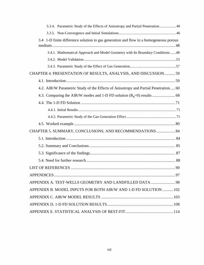
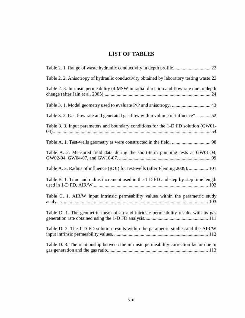


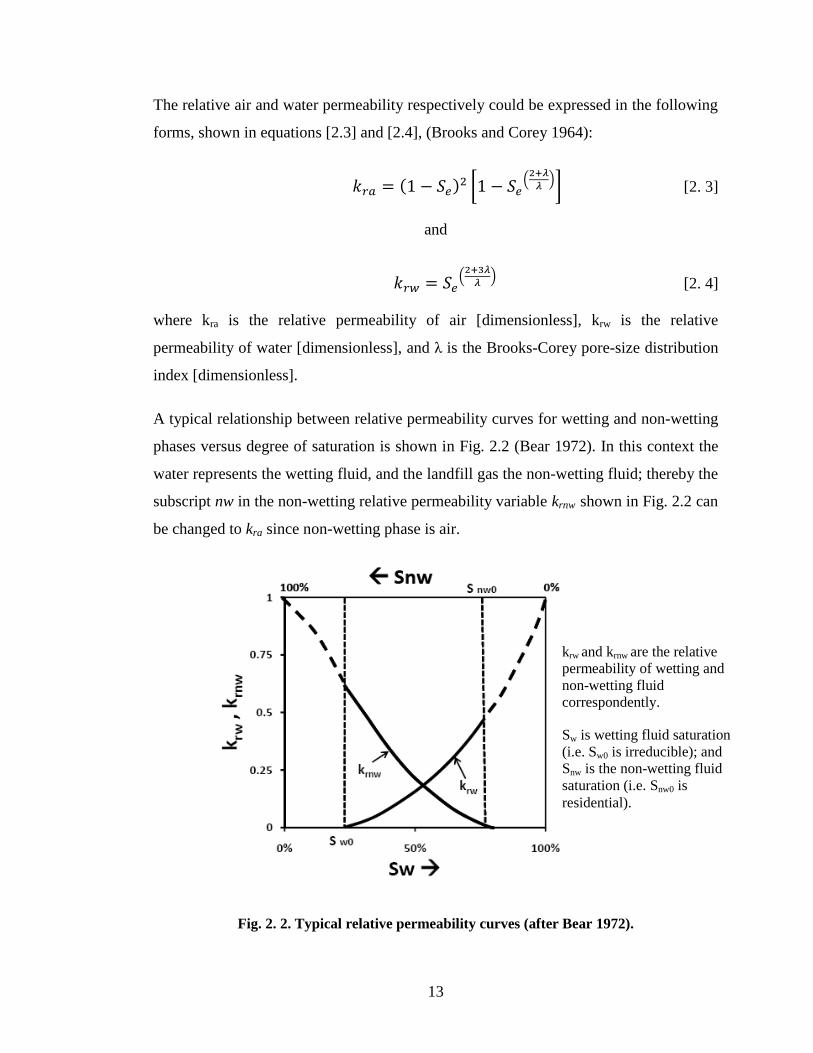


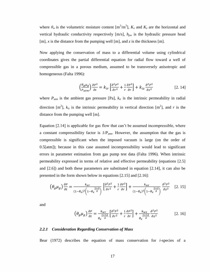

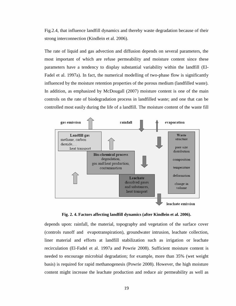


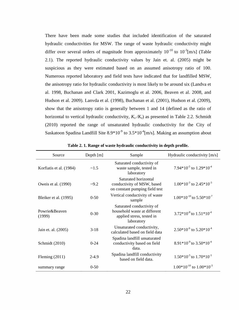
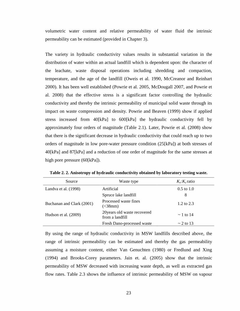
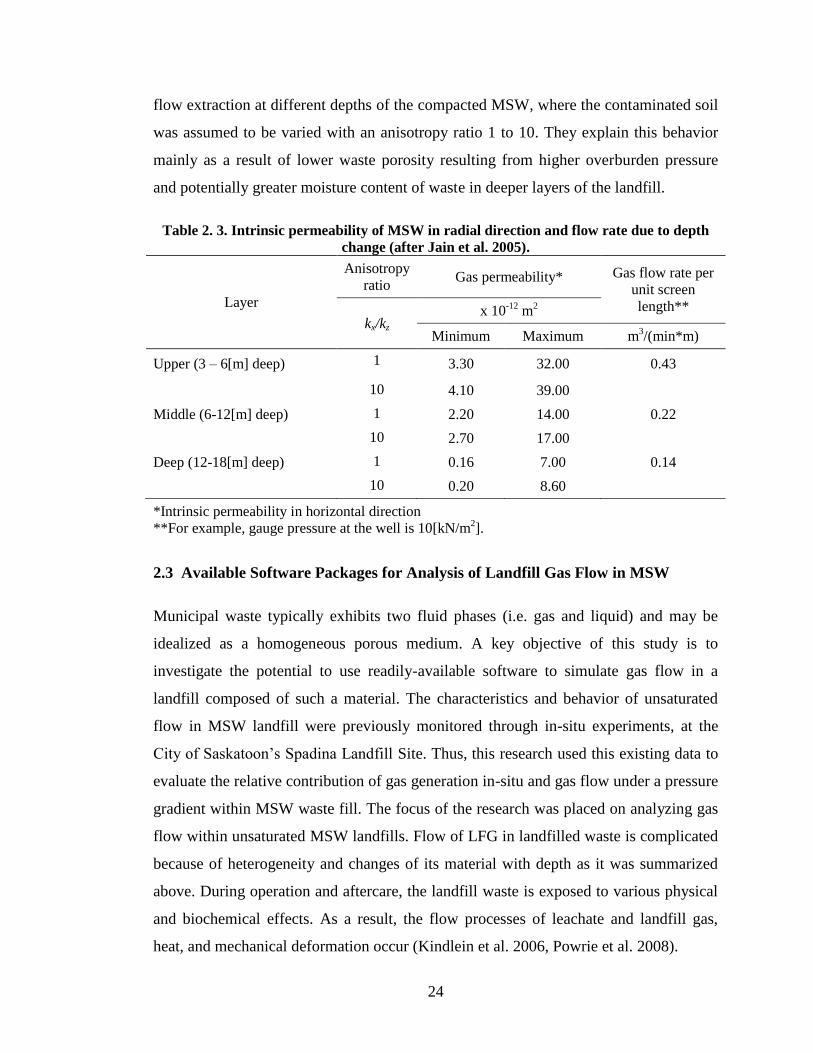


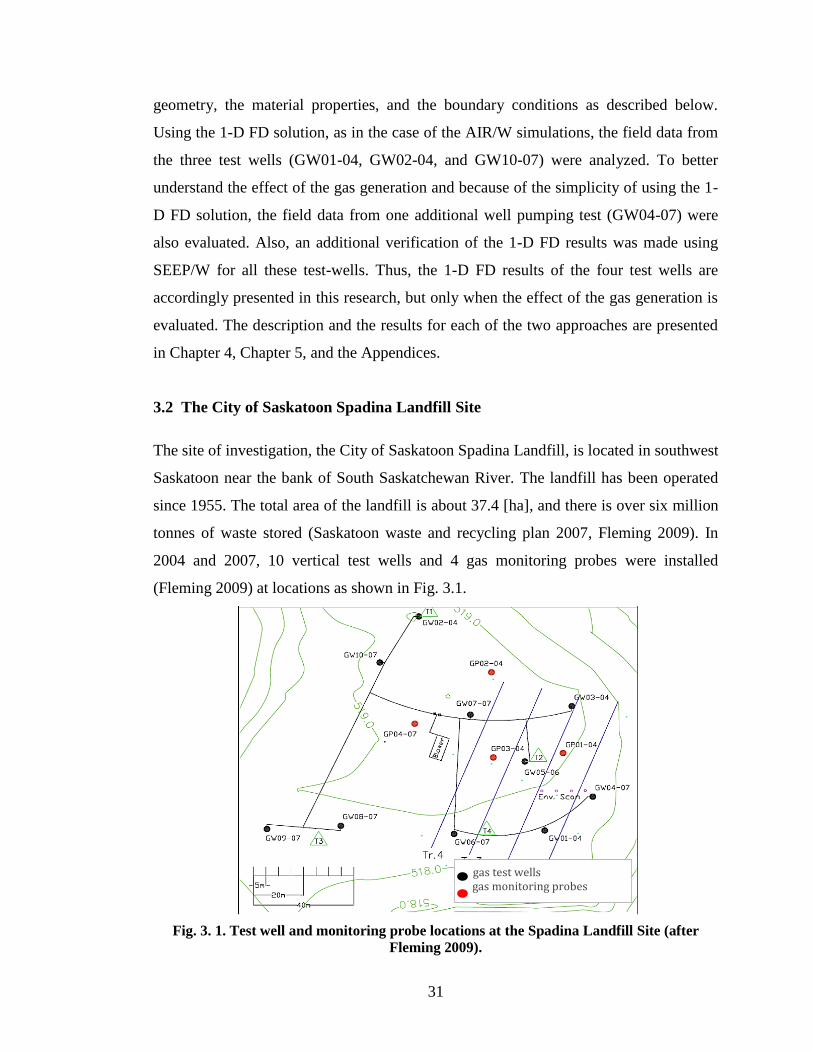
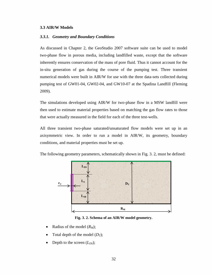


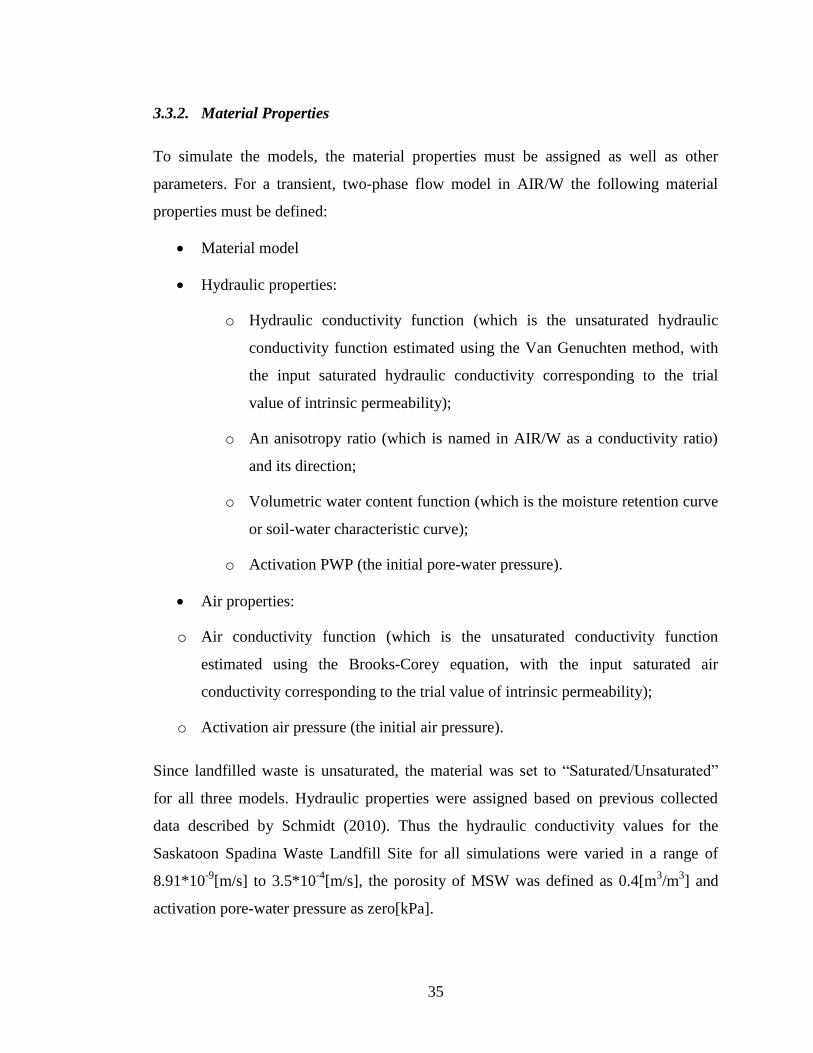
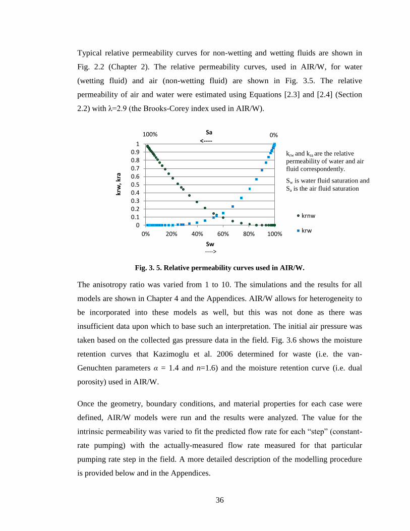


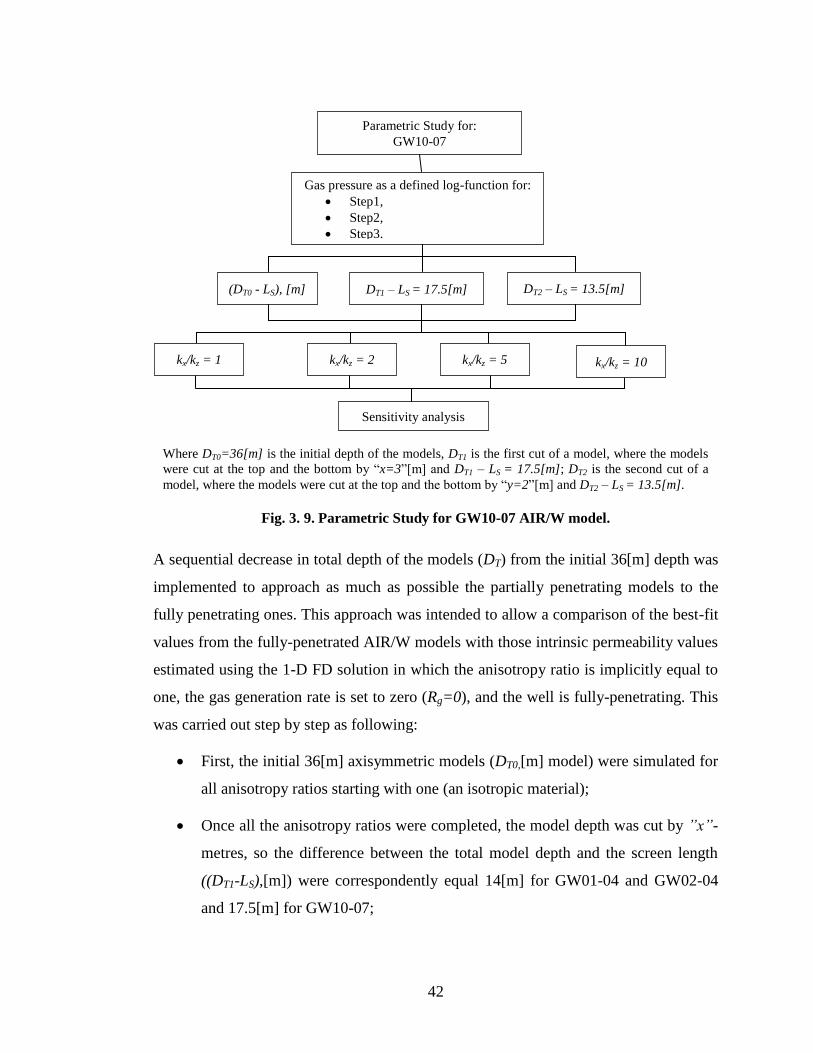
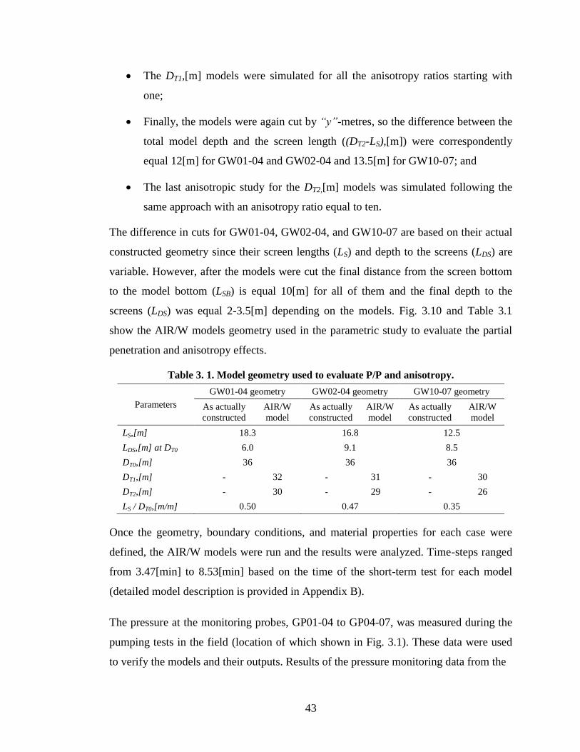
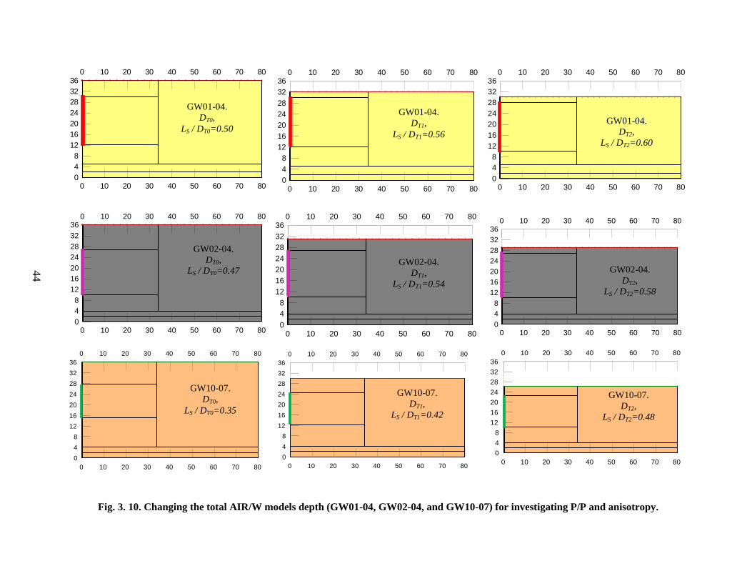


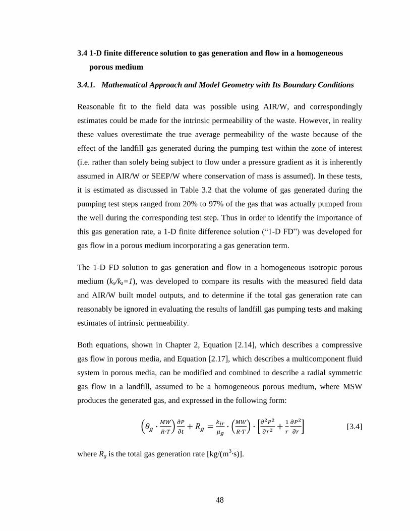


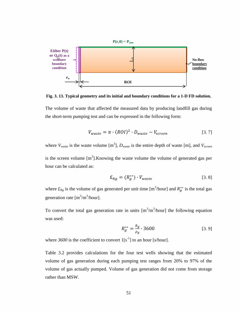

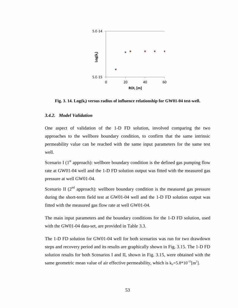


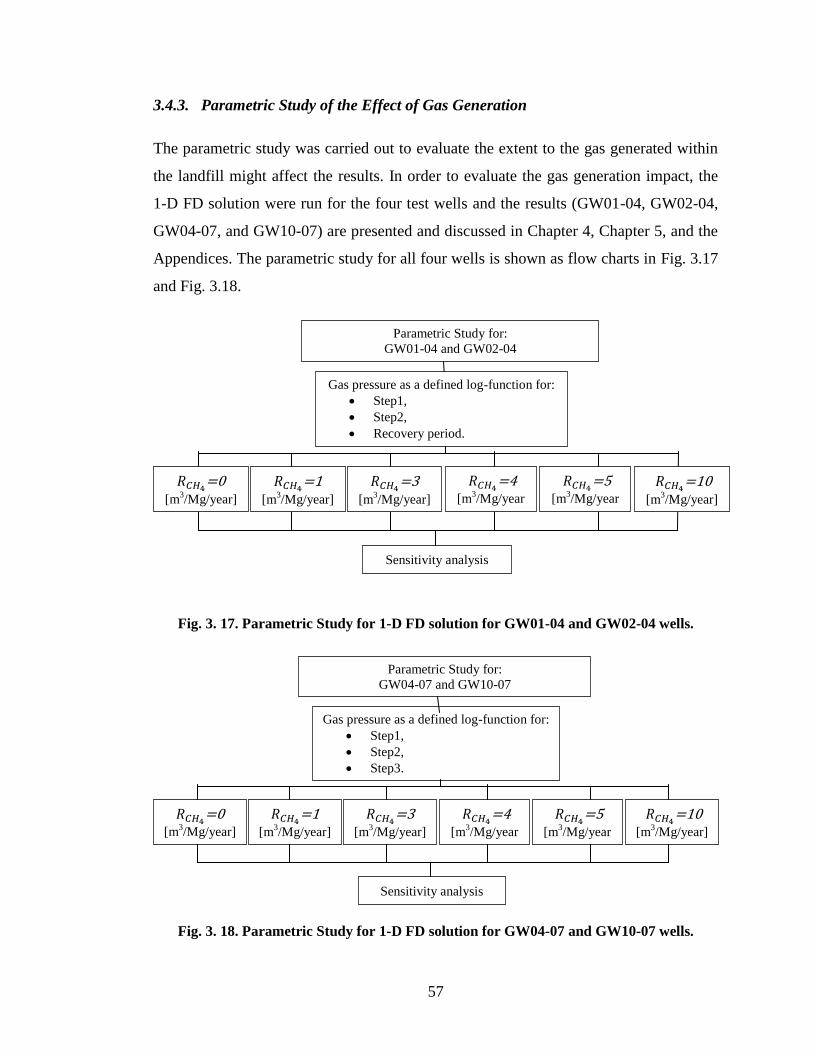
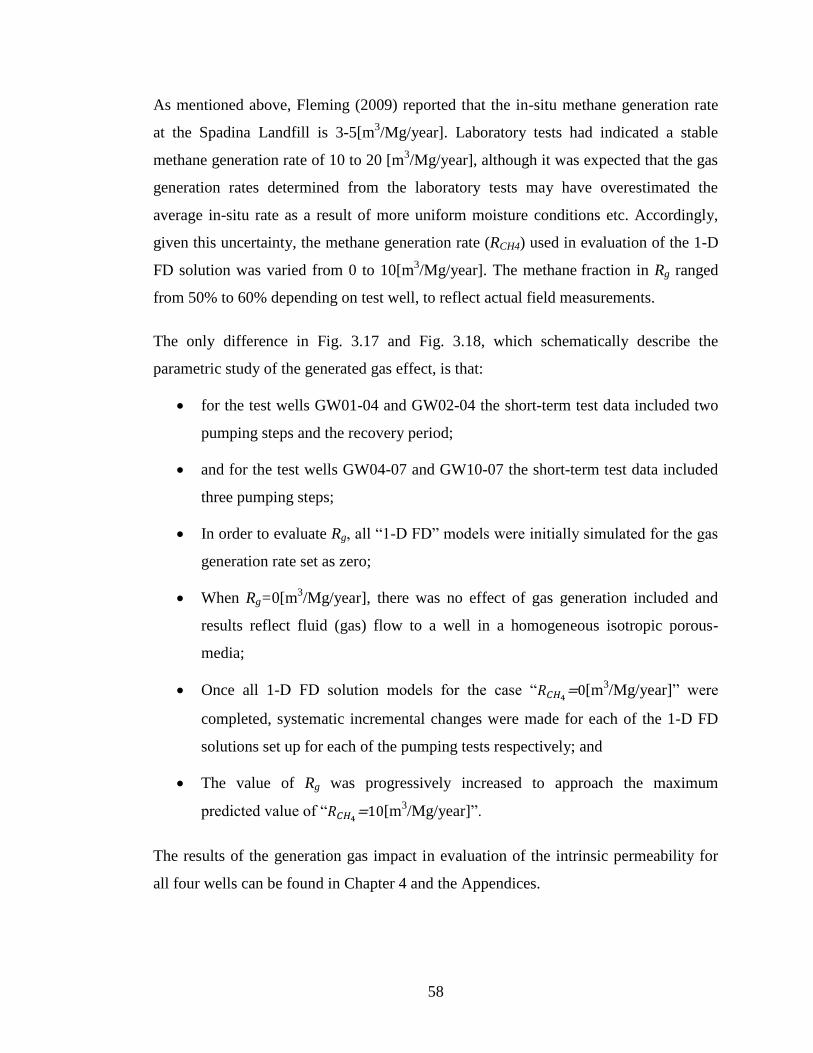

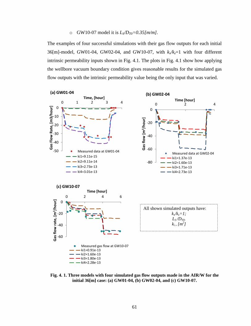

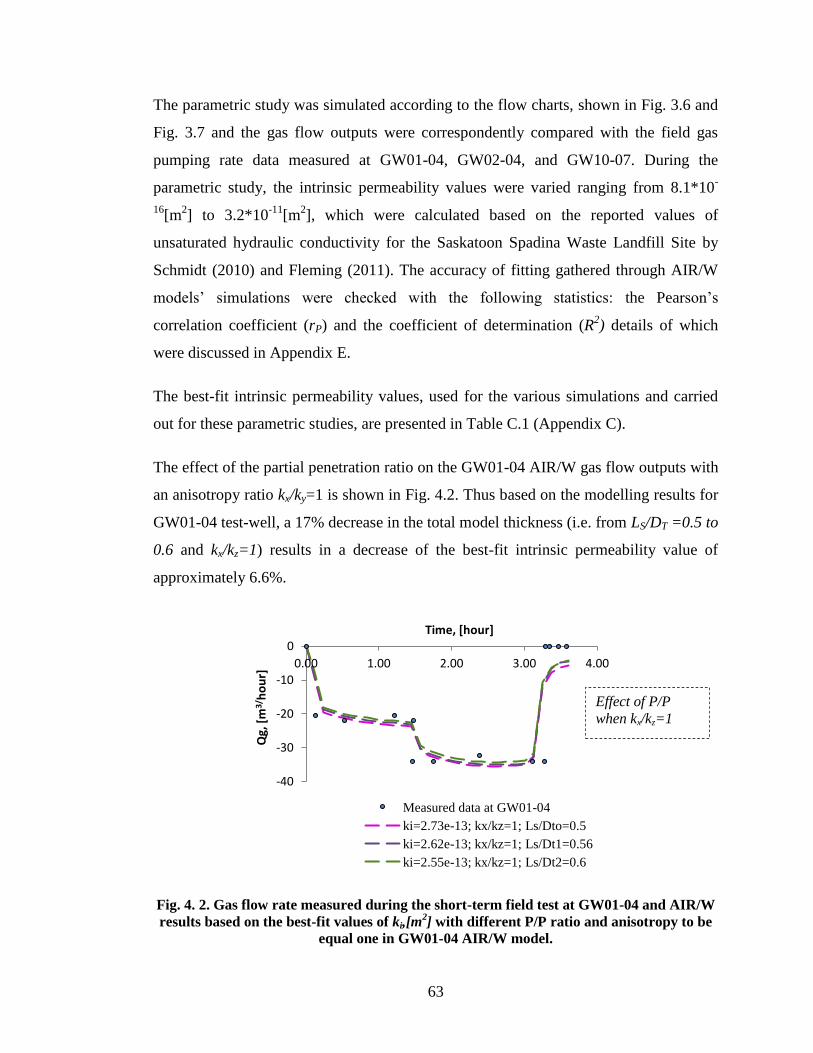
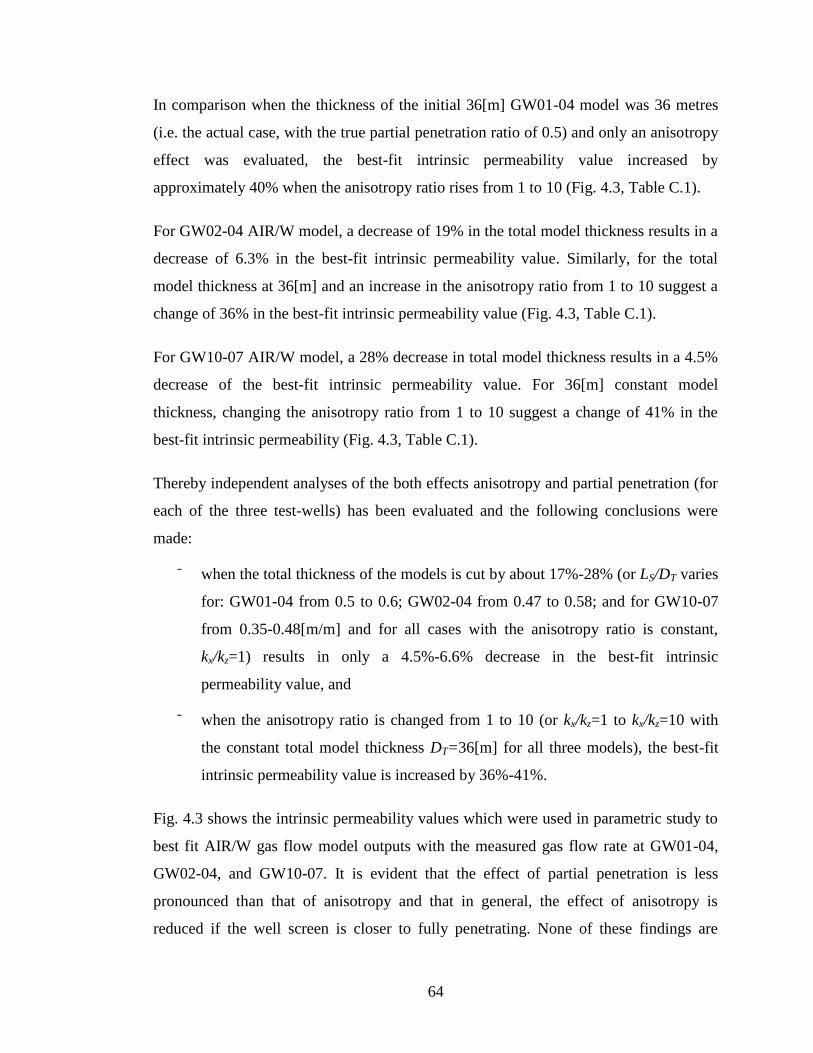

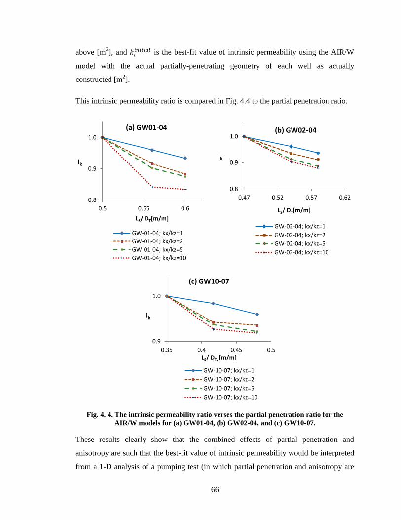
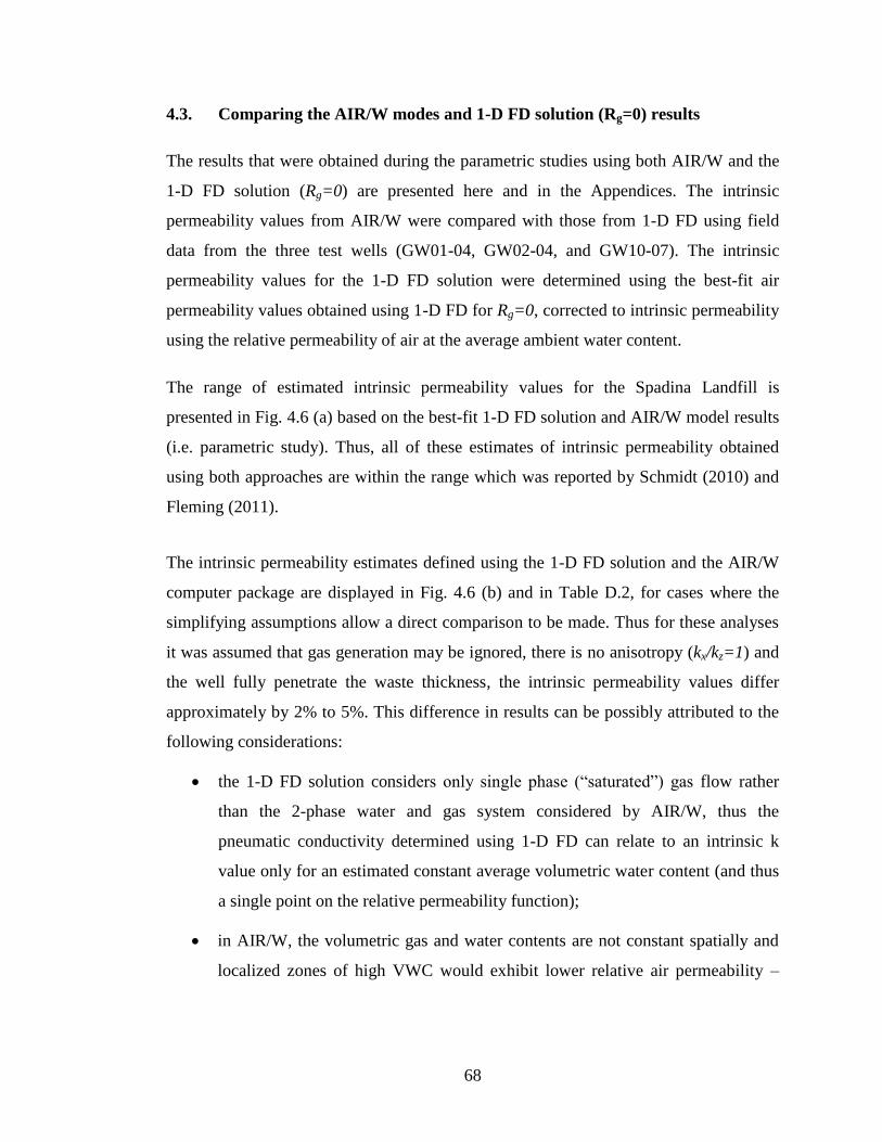


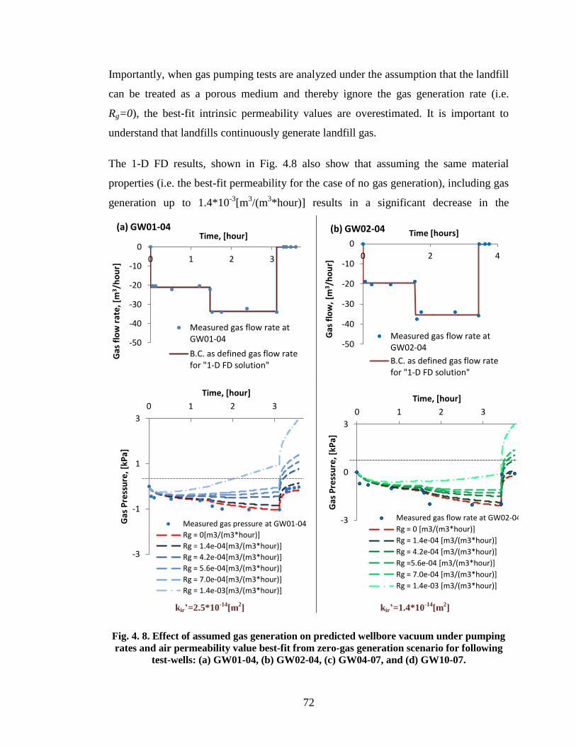
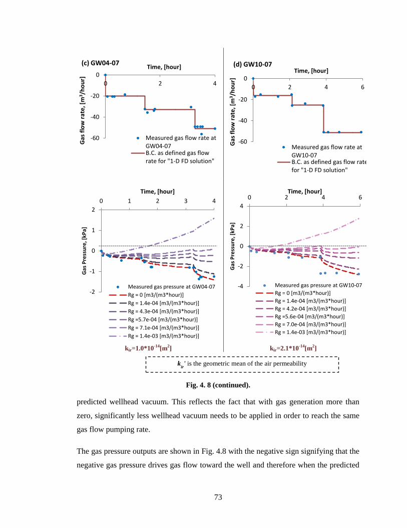

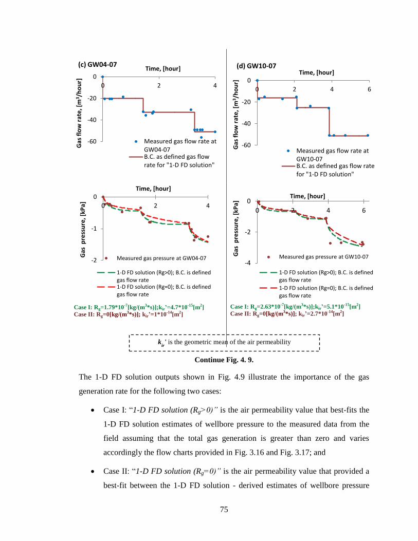


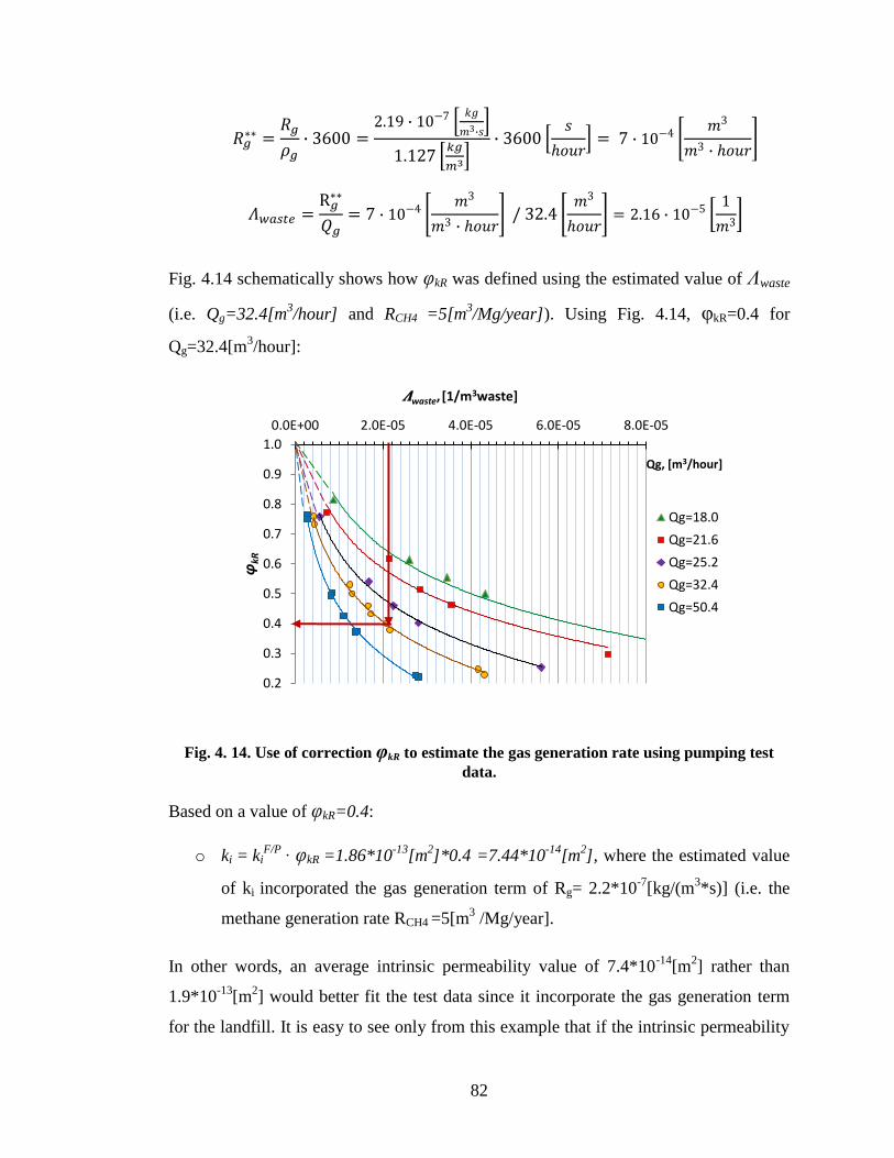


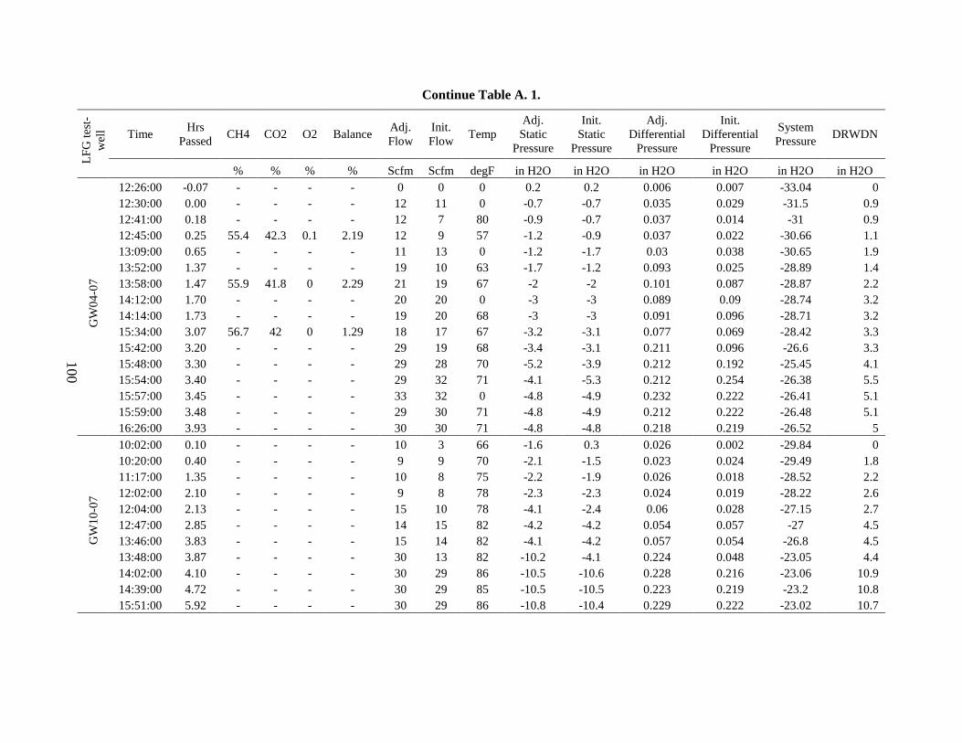
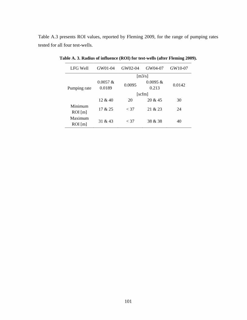


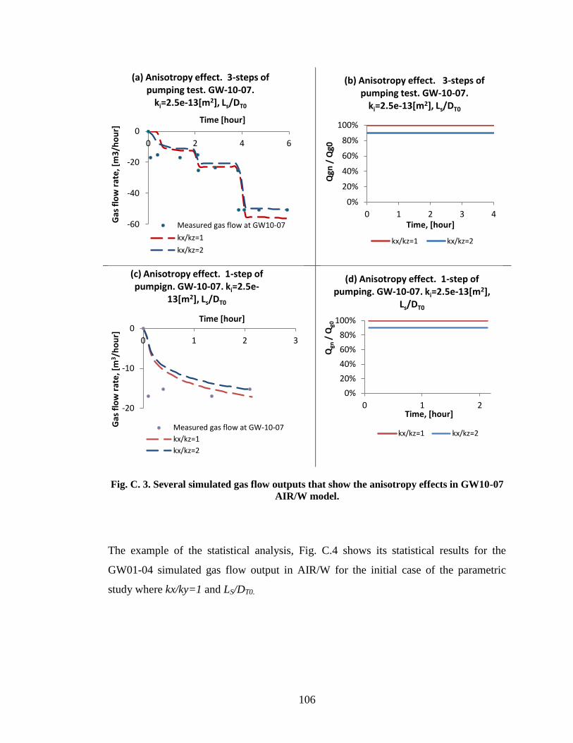


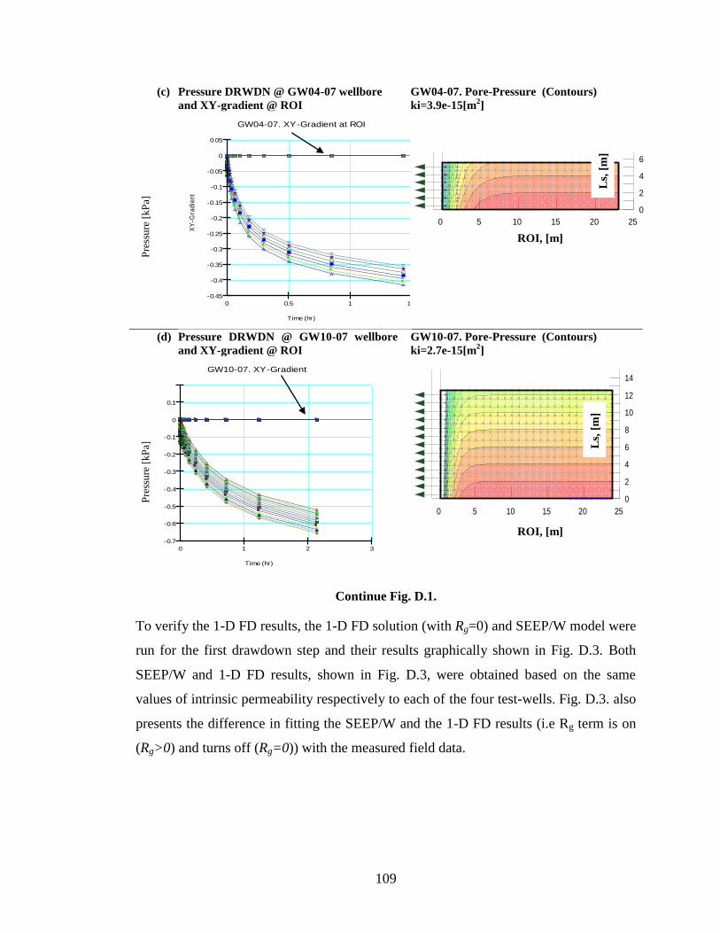


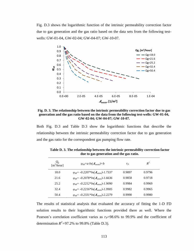
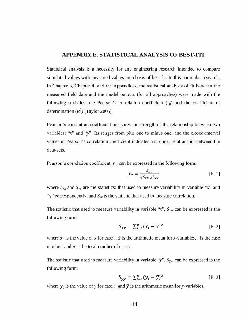


![Municipal Solid Waste Update - Global Methane Initiative...1 Municipal Solid Waste Update [JAPAN] [Kunihiko SHIMADA] GMI Municipal Solid Waste Subcommittee Meeting Vancouver, Canada,](https://static.fdocuments.in/doc/165x107/5e4de36d50ecd14cd3180f83/municipal-solid-waste-update-global-methane-initiative-1-municipal-solid-waste.jpg)


