NUMERICAL ANALYSIS I

by

MARTIN LOTZSchool of Mathematics

The University of Manchester

May 2016

Contents

Contents ii

Week 1 11.1 Computational Complexity . . . . . . . . . . . . . . . . . . . . . . 21.2 Accuracy . . . . . . . . . . . . . . . . . . . . . . . . . . . . . . . 3

Week 2 72.1 Lagrange Interpolation . . . . . . . . . . . . . . . . . . . . . . . . 82.2 Interpolation Error . . . . . . . . . . . . . . . . . . . . . . . . . . 11

Week 3 153.1 Newton’s divided differences . . . . . . . . . . . . . . . . . . . . . 153.2 Convergence . . . . . . . . . . . . . . . . . . . . . . . . . . . . . 183.3 An alternative form . . . . . . . . . . . . . . . . . . . . . . . . . . 20

Week 4 234.1 Integration and Quadrature . . . . . . . . . . . . . . . . . . . . . . 234.2 The Trapezium Rule . . . . . . . . . . . . . . . . . . . . . . . . . 234.3 Simpson’s Rule . . . . . . . . . . . . . . . . . . . . . . . . . . . . 25

Week 5 295.1 The Runge phenomenon revisited . . . . . . . . . . . . . . . . . . 295.2 Composite integration rules . . . . . . . . . . . . . . . . . . . . . . 30

Week 6 356.1 Numerical Linear Algebra . . . . . . . . . . . . . . . . . . . . . . 356.2 The Jacobi and Gauss Seidel methods . . . . . . . . . . . . . . . . 36

Week 7 397.1 Vector Norms . . . . . . . . . . . . . . . . . . . . . . . . . . . . . 41

Week 8 458.1 Matrix norms . . . . . . . . . . . . . . . . . . . . . . . . . . . . . 46

ii

Week 9 539.1 Convergence of Iterative Algorithms . . . . . . . . . . . . . . . . . 549.2 Gershgorin’s circles . . . . . . . . . . . . . . . . . . . . . . . . . . 58

Week 10 6110.1 The Condition Number . . . . . . . . . . . . . . . . . . . . . . . . 6110.2 Nonlinear Equations . . . . . . . . . . . . . . . . . . . . . . . . . 66

Week 11 and 12 7111.1 Fixed-point iterations . . . . . . . . . . . . . . . . . . . . . . . . . 7111.2 Rates of convergence . . . . . . . . . . . . . . . . . . . . . . . . . 7511.3 Newton’s method in the complex plane . . . . . . . . . . . . . . . . 77

Week 1

“Since none of the numbers which we take out fromlogarithmic and trigonometric tables admit of absoluteprecision, but are all to a certain extent approximate only,the results of all calculations performed by the aid ofthese numbers can only be approximately true.”

— C.F. Gauss, Theoria motus corporum coelestium insectionibus conicis solem ambientium, 1809

Classical mathematical analysis owes its existence to the need to model the naturalworld. The study of functions and their properties, of differentiation and integration,has its origins in the attempt to describe how things move and behave. With the riseof technology it became increasingly important to get actual numbers out of formulaeand equations. This is where numerical analysis comes into the scene: to developmethods to make mathematical models based on continuous mathematics effective.

In practice, one often cannot simply plug numbers into formulae and get all theexact results. Most problems require an infinite number of steps to solve, but one onlyhas a finite amount of time available; most numerical data also requires an infiniteamount of storage (just try to store π on a computer!), but a piece of paper or acomputer only has so much space. These are some of the reasons that lead us to workwith approximations.1

An algorithm is a sequence of instructions to be carried out by a computer(machine or human), in order to solve a problem. There are two guiding principles tokeep in mind when designing and analysing numerical algorithms.

1. Computational complexity: algorithms should be fast;

2. Accuracy: solutions should be good.

The first aspect is due to limited time; the second due to limited space. In what follows,we discuss these two aspects in some more detail.

1In discrete mathematics and combinatorics, approximation also becomes a necessity, albeit fora different reason, namely computational complexity. Many combinatorial problems are classified asNP-hard, which makes them computationally intractable.

1

1.1 Computational Complexity

An important consideration in the design of numerical algorithms is efficiency; wewould like to perform computations as fast as possible. Considerable speed-ups arepossible by clever algorithm design that aims to reduce the number of arithmeticoperations needed to perform a task. The measure of “computation time” we use isthe number of basic (floating point) arithmetic operations (+,−,×, /) needed to solvea problem, as a function of the input size. The input size will be typically the numberof values we need to specify the problem.

Example 1.1.1. (Horner’s Algorithms) Take, for example, the problem of evaluatinga polynomial

pn(x) = a0 + a1x+ a2x2 + · · ·+ anx

n

for some x ∈ R and given a0, . . . , an. A naive strategy would be as follows:

1. Compute x, x2, . . . , xn,

2. Multiply akxk for k = 1, . . . , n,

3. Add up all the terms.

If each of the xk is computed individually from scratch, the overall number of multi-plications is n(n+1)/2. This can be improved to 2n−1 multiplications by computingthe powers xk, 1 ≤ k ≤ n, iteratively. An even smarter way, that also uses less inter-mediate storage, can be derived by observing that the polynomial can be written inthe following form:

pn(x) = a0 + x(a1 + a2x+ a3x2 + · · ·+ anx

n−1)

= a0 + xpn−1(x).

The polynomial in brackets has degree n − 1, and once we have evaluated it, weonly need one additional multiplication to have the value of p(x). In the same way,pn−1(x) can be written as pn−1(x) = a1 + xpn−2(x) for a polynomial pn−2(x) ofdegree n−2, and so on. This suggests the possibility of recursion, leading to Horner’sAlgorithm. This algorithms computes a sequence of numbers

bn = an

bn−1 = an−1 + x · bn......

b0 = a0 + x · b1,

where b0 turns out to be the value of the polynomial evaluated at x. In practise, onewould not compute a sequence but overwrite the value of a single variable at eachstep. The following MATLAB and Python code illustrates how the algorithm can beimplemented. Note that MATLAB encodes the coefficients a0, . . . , an as a vector withentries a(1), . . . , a(n+ 1).

f u n c t i o n p = h o r n e r ( a , x )n = l e n g t h ( a ) ;p = a ( n ) ;f o r k=n−1:−1:1

p = a ( k )+ x∗p ;end

MATLAB

def h o r n e r ( po lynomia l , x ) :r e s u l t = 0f o r c o e f f i c i e n t in p o l y n o m i a l :

r e s u l t = r e s u l t ∗x+ c o e f f i c i e n tre turn r e s u l t

Python

This algorithm only requires n multiplications. Horner’s Method is the standardway of evaluating polynomials on computers.

Here we are less concerned with the precise numbers, but with the order ofmagnitude. Thus we will not care so much whether a computation procedure uses1.5n2 operations (n is the input size) or 20n2, but we will care whether the algorithmneeds n3 as opposed to n log(n) arithmetic operations to solve a problem.

To conveniently study the performance of algorithms we use the big-O notation.Given two functions f(n) and g(n) taking integer arguments, we say that

f(n) ∈ O(g(n)) or f(n) = O(g(n)),

if there exists a constant C > 0 and n0 > 0, such that f(n) < C · g(n) for allsufficiently large n > n0. For example, n log(n) = O(n2) and n3 + 10308n ∈ O(n3).

Example 1.1.2. (*) Consider the problem of multiplying a matrix with a vector:

Ax = b,

where A is an n × n matrix, and x and b are n-vectors. Normally, the number ofmultiplications needed is n2, and the number of additions n(n − 1) (verify this!).However, there are some matrices, for example the one with the n-th roots of unityaij = e2πij/n as entries, for which there are algorithms (in this case, the Fast FourierTransform) that can compute the product Ax in O(n log n) operations. This exampleis of great practical importance, but will not be discussed further at the moment.

An interesting and challenging field is algebraic complexity theory, which dealswith lower bounds on the number of arithmetic operations needed to perform certaincomputational tasks. It also asks questions such as whether Horner’s method andother algorithms are optimal, that is, can’t be improved upon.

1.2 Accuracy

In the early 19th century, C.F. Gauss, one of the most influential mathematicians ofall time and a pioneer of numerical analysis, developed the method of least squares inorder to predict the reappearance of the recently discovered asteroid Ceres. He waswell aware of the limitations of numerical computing, as the quote at the beginning ofthis lecture indicates.

Measuring errors

To measure the quality of approximations, we use the concept of relative error. Givena quantity x and a computed approxiamtion x̂, the absolute error is given by

Eabs(x̂) = |x− x̂|,

while the relative error is given as

Erel(x̂) =|x− x̂||x|

.

The benefit of working with relative errors is clear: they are scale invariant. On theother hand, absolute error can be meaningless at time. For example, an error of onehour is irrelevant when estimating the age of Stan the Tyrannosaurus rex at ManchesterMuseum, but it is crucial when determining the time of a lecture. That is because inthe former one hour corresponds to a relative error is of the order 10−11, while in thelatter it is of the order 10−1.

Floating point and significant figures

Nowadays, the established way of representing real numbers on computers is usingfloating-point arithmetic. In the double precision version of the IEEE standard forfloating-point arithmetic, a number is represented using 64 bits.2 A number is written

x = ±f × 2e,

where f is a fraction in [0, 1], represented using 52 bits, and e is the exponent, using11 bits (what is the remaining 64th bit used for?). Two things are worth noticing aboutthis representation: there are largest possible numbers, and there are gaps betweenrepresentable numbers. The largest and smallest numbers representable in this formare of the order of ±10308, enough for most practical purposes. A bigger concern arethe gaps, which means that the results of many computations almost always have tobe rounded to the closest floating-point number.

Throughout this course, when going through calculations without using a com-puter, we will usually use the terminology of significant figures (s.f.) and workwith 4 significant figures in base 10. For example, in base 10,

√3 equals 1.732 to

4 significant figures. To count the number of significant figures in a given number,start with the first non-zero digit from the left and, moving to the right, count allthe digits thereafter, counting final zeros if they are to the right of the decimal point.For example, 1.2048, 12.040, 0.012048, 0.0012040 and 1204.0 all have 5 significantfigures (s.f.). In rounding or truncation of a number to n s.f., the original is replacedby the closest number with with n s.f. An approximation x̂ of a number x is said tobe correct to n significal figures if both x̂ and x round to the same n s.f. number3.

2A bit is a binary digit, that is, either 0 or 1.3This definition is not without problems, see for example the discussion in Section 1.2 of Nicholas J.

Higham, Accuracy and Stability of Numerical Algorithms, SIAM 2002

Remark 1.2.1. Note that final zeros to left of the decimal point may or may not besignificant: the number 1204000 has a least 4 significant figures, but without anymore information there is no way of knowing whether or not any more figures aresignificant. When 1203970 is rounded to 5 significant figures to give 1204000, anexplanation that this has 5 significant figures is required. This could be made clear bywriting it in scientific notation: 1.2040× 106. In some cases we also have to agreewhether to round up or round down: for example, 1.25 could equal 1.2 or 1.3 to twosignificant figures. If we agree on rounding up, then to say that a = 1.2048 to 5 s.f.means that the exact value of a satisfies 1.20475 ≤ a < 1.40485.

Example 1.2.2. Suppose we want to find the solution to the quadratic equation

ax2 + bx+ c = 0.

The two solutions to this problem are given by

x1 =−b+

√b2 − 4ac

2a, x2 =

−b−√b2 − 4ac

2a. (1.2.1)

In principle, to find x1 and x2 one only needs to evaluate the expressions for givena, b, c. Assume, however, that we are only allowed to compute to four significantfigures, and consider the particular equation

x2 + 39.7x+ 0.13 = 0.

Using the formula 1.2.1, we have, always rounding to four significant figures,

a = 1, b = 39.7, c = 0.13,

b2 = 1576.09 = 1576 (to 4 s.f.) , 4ac = 0.52 (to 4 s.f.),

b2 − 4ac = 1575.48 = 1575 (to 4 s.f.) ,√b2 − 4ac = 39.69.

Hence, the computed solutions (to 4 significant figures) are given by

x1 = −0.005, x2 = −39.69

The exact solutions, however, are

x1 = −0.0032748..., x2 = −39.6907...

The solution x1 is completely wrong, at least if we look at the relative error:

|x1 − x1||x1|

= 0.5268.

While the accuracy can be increased by increasing the number of significant figuresduring the calculation, such effects happen all the time in scientific computing and

the possibility of such effects has to be taken into account when designing numericalalgorithms.

Note that it makes sense, as in the above example, to look at errors in a relativesense. An error of one mile is certainly negligible when dealing with astronomicaldistances, but not so when measuring the length of a race track.

By analysing what causes the error it is sometimes possible to modify the methodof calculation in order to improve the result. In the present example, the problems arebeing caused by the fact that b ≈

√b2 − 4ac, and therefore

−b+√b2 − 4ac

2a=−39.7 + 39.69

2

causes what is called “catastrophic cancellation”. A way out is provided by theobservation that the two solutions are related by

x1 · x2 =c

a. (1.2.2)

When b > 0, the calculation of x2 according to (1.2.1) shouldn’t cause any problems,in our case we get−39.69 to four significant figures. We can then use (1.2.2) to derivex1 = c/(ax2) = −0.00327.

Sources of errors

As we have seen, one can get around numerical catastrophes by choosing a clevermethod for solving a problem, rather than increasing precision. So far we haveconsidered errors introduced due to rounding operations. There are other sources oferrors:

1. Overflow

2. Errors in the model

3. Human or measurements errors

4. Truncation or approximation errors

The first is rarely an issue, as we can represent numbers of order 10308 on a com-puter. The second two are important factors, but fall outside the scope of this lecture.The third has to do with the fact that many computations are done approximatelyrather than exactly. For computing the exponential, for example, we might use amethod that gives the approximation

ex ≈ 1 + x+x2

2.

As it turns out, many practical methods give approximations to the “true” solution.

Week 2

How do we represent a function on a computer? If f is a polynomial of degree n,

f(x) = pn(x) = a0 + a1x+ · · ·+ anxn

then we only need to store the n+ 1 coefficients a0, . . . , an. In fact, one can approx-imate an arbitrary continuous function on a bounded interval by a polynomial. Recallthat Ck([a, b]) is the set of functions that are k times continuously differentiable [a, b].

Theorem 2.0.1 (Weierstrass). For any f ∈ C([0, 1]) and any ε > 0 there exists apolynomial p(x) such that

max0≤x≤1

|f(x)− p(x)| ≤ ε.

Given pairs (xj , yj) ∈ R, 0 ≤ j ≤ n, with distinct xj , the interpolation problemconsists of finding a polynomial p of smallest possible degree such that

p(xj) = yj , 0 ≤ j ≤ n. (2.0.1)

0 1 2 3 4 5 6 76

8

10

12

14

16

18

20

22

Figure 2.1: The interpolation problem.

7

Example 2.0.2. Let h = 1/n, x0 = 0, and xi = ih for 1 ≤ i ≤ n. The xi subdividethe interval [0, 1] into segments of equal length h. Now let yi = ih/2 for 0 ≤ i ≤ n.Then the points (xi, yi) all lie on the line p1(x) = x/2, as is easily verified. It is alsoeasy to see that p1 is the unique polynomial of degree at most 1 that goes throughthese points. In fact, we will see that it is the unique polynomial of degree at most nthat passes through these points!

We will first describe the method of Lagrange interpolation, which also helps to es-tablish the existence and uniqueness of an interpolation polynomial satisfying (2.0.1).We then discuss the quality of approximating polynomials by interpolation, the ques-tion of convergence, as well as other methods such as Newton interpolation.

2.1 Lagrange Interpolation

The next lemma shows that it is indeed possible to find a polynomial of degree atmost n satisfying (2.0.1). We denote by Pn the set of all polynomials of degreeat most n. Note that this also includes polynomials of degree smaller than n, andin particular constants, since we allow coefficients such as an in the representationa0 + a1x+ · · ·+ anx

n to be zero.

Lemma 2.1.1. Let x0, x1, . . . , xn be distinct real numbers. Then there exist polyno-mials Lk ∈ Pn such that

Lk(xj) =

{1 j = k,

0 j 6= k

Moreover, the polynomial

pn(x) =n∑k=0

Lk(x)yk

is in Pn and satisfies pn(xj) = yj for 0 ≤ j ≤ n.

Proof. Clearly, if Lk exists, then it is a polynomial of degree n with n roots at xj forj 6= k. Hence, it factors as

Lk(x) = Ck∏j 6=k

(x− xj) = Ck(x− x0) · · · (x− xj−1)(x− xj+1) · · · (x− xn)

for a constant Ck. To determine Ck, set x = xk. Then Lk(xk) = 1 = Ck∏j 6=k(xk −

xj) and therefore

Ck =1∏

j 6=k(xk − xj).

Note that we assumed the xj to be distinct, otherwise we would have to divide by zeroand cause a disaster. We therefore get the representation

Lk(x) =

∏j 6=k(x− xj)∏j 6=k(xk − xj)

.

This proves the first claim. Now set

pn(x) :=

n∑k=0

ykLk(x).

Then pn(xj) =∑n

k=0 ykLk(xj) = yjLj(xj) = yj . Since pn(x) is a linear combina-tions of the various Lk, it lives in Pn. This completes the proof.

We have shown the existence of an interpolating polynomial. We next show thatthis polynomial is uniquely determined. The important ingredient is the FundamentalTheorem of Algebra, a version of which states that

A polynomial of degree n with complex coefficients has exactly n com-plex roots.

Theorem 2.1.2 (Lagrange Interpolation Theorem). Let n ≥ 0. Let xj , 0 ≤ j ≤ n, bedistinct real numbers and let yj , 0 ≤ j ≤ n, be any real numbers. Then there exists aunique pn(x) ∈ Pn such that

pn(xj) = yj , 0 ≤ j ≤ n. (2.1.1)

Proof. The case n = 0 is clear, so let us assume n ≥ 1. In Lemma 2.1.1 we construc-ted a polynomial pn(x) of degree at most n satisfying the conditions (2.1.1), provingthe existence part. For the uniqueness, assume that we have two such polynomialspn(x) and qn(x) of degree at most n satisfying the interpolating property (2.1.1). Thegoal is to show that they are the same. By assumption, the difference pn(x)−qn(x) is apolynomial of degree at most n that takes on the value pn(xj)−qn(xj) = yj−yj = 0at the n + 1 distinct xj , 0 ≤ j ≤ n. By the Fundamental Theorem of Algebra, anon-zero polynomial of degree n can have no more than n distinct real roots, fromwhich it follows that pn(x)− qn(x) ≡ 0, or pn(x) = qn(x).

Definition 2.1.3. Given n + 1 distinct real numbers xj , 0 ≤ j ≤ n, and n + 1 realnumbers yj , 0 ≤ j ≤ n, the polynomial

pn(x) =

n∑k=0

Lk(x)yk (2.1.2)

is called the Lagrange interpolation polynomial of degree n corresponding to thedata points (xj , yj), 0 ≤ j ≤ n. If the yk are the values of a function f , that is, iff(xk) = yk, 0 ≤ k ≤ n, then pn(x) is called the Lagrange interpolation polynomialassociated to f and x0, . . . , xn.

Remark 2.1.4. Note that the interpolation polynomial is uniquely determined, butthat the polynomial can be written in different ways. The term Lagrange interpolation

polynomial thus referes to to the particular form (2.1.2) of this polynomial. Forexample, the two expressions

q2(x) = x2, p2(x) =x(x− 1)

2+x(x+ 1)

2

define the same polynomial (as can be verified by multiplying out the terms onthe right), and thus both represent the unique polynomial interpolating the points(x0, y0) = (−1, 1), (x1, y1) = (0, 0), (x2, y2) = (1, 1), but only p2(x) is in theLagrange form.

(*) A different take on the uniqueness problem can be arrived at by translating theproblem into a linear algebra one. For this, note that if pn(x) = a0+a1x+ · · ·+anxn,then the polynomial evaluation problem at the xj , 0 ≤ j ≤ n, can be written as amatrix vector product:

y0y1...yn

=

1 x0 · · · xn01 x1 · · · xn1...

.... . .

...1 xn · · · xnn

a0a1...an

,

or y = Xa. If the matrix X is invertible, then the interpolating polynomial isuniquely determined by the coefficient vector a = X−1y. The matrix X is invertibleif and only if det(X) 6= 0. The determinant of X is the well-known Vandermondedeterminant:

det(X) = det

1 x0 · · · xn01 x1 · · · xn1...

.... . .

...1 xn · · · xnn

=∏j>i

(xj − xi).

Clearly, this determinant is different from zero if and only if the xj are all distinct,which shows the importance of this assumption.

Example 2.1.5. Consider the function f(x) = ex on the interval [−1, 1], with inter-polation points x0 = −1, x1 = 0, x2 = 1. The Lagrange basis functions are

L0(x) =(x− x1)(x− x2)

(x0 − x1)(x0 − x2)=

1

2x(x− 1),

L1(x) = 1− x2,

L2(x) =1

2x(x+ 1).

The Lagrange interpolation polynomial is therefore given by

p2(x) =1

2x(x− 1)e−1 + (1− x2)e0 +

1

2x(x+ 1)e1

= 1 + x sinh(1) + x2(cosh(1)− 1).

−1 −0.8 −0.6 −0.4 −0.2 0 0.2 0.4 0.6 0.8 10

0.5

1

1.5

2

2.5

3

Figure 2.2: Lagrange interpolation of ex at −1, 0, 1.

2.2 Interpolation Error

If the data points (xj , yj) come from a function f(x), that is, if f(xj) = yj , thenthe Lagrange interpolating polynomial can look very different from the originalfunction. It is therefore of interest to have some control over the interpolation errorf(x) − pn(x). Clearly, without any further assumption on f the difference can bearbitrary. We will therefore restrict to function f that are sufficiently smooth, asquantified by belonging to some class Ck([a, b]) for sufficiently large k.

Example 2.2.1. All polynomials belong to Ck([a, b]) for all bounded intervals [a, b]and any integer k ≥ 0. However, f(x) = 1/x 6∈ C([0, 1]), as f(x)→∞ for x→ 0and the function is therefore not continuous there.

Now that we have established the existence and uniqueness of the interpolationpolynomial, we would like know how well it approximates the function.

Theorem 2.2.2. Let n ≥ 0 and assume f ∈ Cn+1([a, b]). Let pn(x) ∈ Pn be theLagrange interpolation polynomial associated to f and distinct xj , 0 ≤ j ≤ n. Thenfor every x ∈ [a, b] there exists ξ = ξ(x) ∈ (a, b) such that

f(x)− pn(x) =f (n+1)(ξ)

(n+ 1)!πn+1(x), (2.2.1)

whereπn+1(x) = (x− x0) · · · (x− xn).

For the proof of Theorem 2.2.2 we need the following consequence of Rolle’sTheorem.

Lemma 2.2.3. Let f ∈ Cn([a, b]), and suppose f vanishes at n+1 points x0, . . . , xn.Then there exists ξ ∈ (a, b) such that the n-th derivative f (n)(x) satisfies f (n)(ξ) = 0.

Proof. By Rolle’s Theorem, for any two xi, xj there exists a point in between wheref ′ vanishes, therefore f ′ vanishes at (at least) n points. Repeating this argument, itfollows that f (n) vanishes at some point ξ ∈ (a, b).

Proof of Theorem 2.2.2. Assume x 6= xj for 0 ≤ j ≤ n (otherwise the theorem isclearly true). Define the function

ϕ(t) = f(t)− pn(t)− f(x)− pn(x)

πn+1(x)πn+1(t).

This function vanishes at n + 2 distinct points, namely t = xj , 0 ≤ j ≤ n, and x.Assume n > 0 (the case n = 0 is left as an exercise). By Lemma 2.2.3, the functionϕ(n+1) has a zero ξ ∈ (a, b), while the (n+ 1)-st derivative of pn vanishes (since pnis a polynomial of degree n). We therefore have

0 = ϕ(n+1)(ξ) = f (n+1)(ξ)− f(x)− pn(x)

πn+1(x)(n+ 1)!,

from which we get

f(x)− pn(x) =f (n+1)(ξ)

(n+ 1)!πn+1(x).

This completes the proof.

Theorem 2.2.2 contains an unspecified number ξ. Even though we can’t find thislocation in practise, the situation is not too bad as we can sometimes upper-bound the(n+ 1)-st derivative of f on the interval [a, b].

Corollary 2.2.4. Under the conditions as in Theorem 2.2.2,

|f(x)− pn(x)| ≤ Mn+1

(n+ 1)!|πn+1(x)|,

whereMn+1 = max

a≤x≤b|f (n+1)(x)|.

Proof. By assumption we have the bound

|f (n+1)(ξ)| ≤Mn+1,

so that

|f(x)− pn(x)| ≤

∣∣∣∣∣f (n+1)(ξ)πn+1(x)

(n+ 1)!

∣∣∣∣∣ ≤Mn+1|πn+1(x)|(n+ 1)!

.

This completes the proof.

Example 2.2.5. Suppose we would like to approximate f(x) = ex by an interpolatingpolynomial p1 ∈ P1 at points x0, x1 ∈ [0, 1] that are separated by a distance h =x1 − x0. What h should we choose to achieve

|p1(x)− ex| ≤ 10−5, x0 ≤ x ≤ x1.

From Corollary 2.2.4, we get

|p1(x)− ex| ≤ M2|π2(x)|2

,

where M2 = maxx0≤x≤x1 |f (2)(x)| ≤ e (because x0, x1 ∈ [0, 1] and f (2)(x) = ex)and π2(x) = (x− x0)(x− x1). To find the maximum of π2(x), first write

x = x0 + θh, x1 = x0 + h.

for θ ∈ [0, 1]. Then

|π2(x)| = θh(h− θh) = h2θ(1− θ).

By taking derivatives with respect to θ we find that the maximum is attained atθ = 1/2. Hence,

π2(x) ≤ h2 1

2

(1− 1

2

)=h2

4.

We conclude that

|p1(x)− ex| ≤ h2e

8.

In order to achieve that this falls below 10−5 we require that h ≤√

8 · 10−5/e =5.425 · 10−3. This gives information on how big the spacing of points needs to be forlinear interpolation to achieve a certain accuracy.

Week 3

While the interpolation polynomial of degree at most n for a function f and n + 1points x0, . . . , xn is unique, it can appear in different forms. The one we have seen sofar is the Lagrange form, where the polynomial is given as a linear combination of theLagrange basis functions:

p(x) =n∑k=0

Lk(x)f(xk),

or some modifications of this form, such as the barycentric form (see Section 3.3). Adifferent approach to constructing the interpolation polynomial is based on Newton’sdivided differences.

3.1 Newton’s divided differences

A convenient way of representing an interpolation polynomial is as

p(x) = a0 + a1(x− x0) + · · ·+ an(x− x0) · · · (x− xn−1). (3.1.1)

Provided we have the coefficients a0, . . . , an, evaluating the polynomial only requiresn multiplications using Horner’s Method. Moreover, it is easy to add new points: ifxn+1 is added, the coefficients a0, . . . , an don’t need to be changed.

Example 3.1.1. Let x0 = −1, x1 = 0, x2 = 1 and x3 = 2. Then the polynomialp3(x) = x3 can be written in the form (3.1.1) as

p3(x) = x3 = −1 + (x+ 1) + (x+ 1)x(x− 1).

A pleasant feature of the form (3.1.1) is that the coefficients a0, . . . , an can becomputed easily using divided differences. The divided differences associated to thefunction f and distinct x0, . . . , xn ∈ R are defined recursively as

f [xi] := f(xi),

f [xi, xi+1] :=f [xi+1]− f [xi]

xi+1 − xi,

f [xi, xi+1, . . . , xi+k] : =f [xi+1, xi+2, . . . , xi+k]− f [xi, xi+1, . . . , xi+k−1]

xi+k − xi.

15

The divided differences can be computed from a divided difference table, wherewe move from one column to the next by applying the rules above (here we use theshorthand fi := f(xi)):

x0 f0f [x0, x1]

x1 f1 f [x0, x1, x2]f [x1, x2] f [x0, x1, x2, x3]

x2 f2 f [x1, x2, x3]f [x2, x3]

x3 f3

From this table we also see that adding a new pair (xn+1, fn+1) would require anupdate of the table that takes O(n) operations.

Theorem 3.1.2. Let x0, . . . , xn be distinct points. Then the interpolation polynomialfor f at points xi, . . . , xi+k is given by

pi,k(x) = f [xi] + f [xi, xi+1](x− xi) + f [xi, xi+1, xi+2](x− xi)(x− xi+1) + · · ·+ f [xi, . . . , xi+k](x− xi) · · · (x− xi+k−1).

In particular, the coefficients in Equation (3.1.1) are given by the divided differences

ak = f [x0, . . . , xk],

and the interpolation polynomial pn(x) can therefore be written as

pn(x) = p0,n(x) = f [x0] + f [x0, x1](x− x0) + f [x0, x1, x2](x− x0)(x− x1) + · · ·+ f [x0, . . . , xn](x− x0) · · · (x− xn−1).

Before going into the proof, observe that the divided difference f [x0, . . . , xn]is the highest order coefficient, that is, the coefficient of xn, of the interpolationpolynomial xn. This observation is crucial in the proof.

Proof. ∗ The proof is by induction on k. For the case k = 0 we have pi,0(x) =f [xi] = f(xi), which is the unique interpolation polynomial of degree 0 at (xi, f(xi)),so the claim is true in this case. Assume the statement holds for k > 0, which meansthat the interpolation polynomial pi,k(x) for the pairs (xi, f(xi)), . . . , (xi+k, f(xi+k))is given as in the theorem. We can now choose a value ak+1 such that

pi,k+1(x) = pi,k(x) + ak+1(x− xi) . . . (x− xi+k) (3.1.2)

interpolates f at xi, . . . , xi+k+1. In fact, note that pi,k+1(xj) = f(xj) for i ≤ j ≤i+ k, so that we only require ak+1 to be chosen so that pi,k+1(xi+k+1) = f(xi+k+1).Moreover, note that ak+1 is the coefficient of highest order of pi,k+1(x), that is, wecan write

pi,k+1(x) = ak+1xk+1 + lower order terms.

The only thing that needs to be shown is that ak+1 = f [xi, . . . , xi+k+1]. For this,we define a new polynomial q(x), show that it coincides with pi,k+1(x) by beingthe unique interpolation polynomial of f at xi, . . . , xi+k+1, and then show that thehighest order coefficient of q(x) is precisely f [xi, . . . , xi+k+1]. Define

q(x) =(x− xi)pi+1,k(x)− (x− xi+k+1)pi,k(x)

xi+k+1 − xi. (3.1.3)

This polynomial has degree ≤ k + 1, just like pi,k+1(x). Moreover:

q(xi) = pi,k(xi) = f(xi)

q(xi+k+1) = pi+1,k(xi+k+1) = f(xi+k+1)

q(xj) =(xj − xi)f(xj)− (xj − xi+k+1)f(xj)

xi+k+1 − xi= f(xj), i+ 1 ≤ j ≤ i+ k.

This means that q(x) also interpolates f at xi, . . . , xi+k+1, and by the uniqueness ofthe interpolation polynomial, must equal pi,k+1(x). Let’s now compare the coefficientsof xk+1 in both polynomials. The coefficient of xk+1 in pi,k+1 is ak+1, as can beseen from (3.1.2). By the induction hypothesis, the polynomials pi+1,k(x) and pi,k(x)have the form

pi+1,k(x) = f [xi+1, . . . , xk+i+1]xk + lower order terms ,

pi,k(x) = f [xi, . . . , xk+i]xk + lower order terms .

By plugging into (3.1.3), we see that the coefficient of xk+1 in q(x) is

f [xi+1, . . . , xi+k+1]− f [xi, . . . , xi+k]

xi+k+1 − xi= f [xi, . . . , xi+k+1].

This coefficient has to equal ak+1, and the claim follows.

Example 3.1.3. Let’s find the divided difference form of a cubic interpolation poly-nomial for the points

(−1, 1), (0, 1), (3, 181), (−2,−39).

The divided difference table would look like

j xj fj f [xj , xj+1] f [xj , xj+1, xj+2] f [x0, x1, x2, x3]

0 −1 10

1 0 1 60−03−(−1) = 15

181−13−0 = 60 8−15

−2−(−1) = 7

2 3 181 44−60−2−0 = 8

−39−181−2−3 = 44

3 −2 −39

(3.1.4)

The coefficients aj = f [x0, . . . , xj ] are given by the upper diagonal, the interpolationpolynomial is thus

p3(x) = a0 + a1(x− x0) + a2(x− x0)(x− x1) + a3(x− x0)(x− x1)(x− x2)= 1 + 15x(x+ 1) + 7x(x+ 1)(x− 3).

Now suppose we add another data point (4, 801). This amounts to adding only onenew term to the polynomial. The new coefficient a4 = f [x0, . . . , x4] is calculated byadding a new line at the bottom of Table (3.1.4) as follows:

f4 = 801, f [x3, x4] = 140, f [x2, x3, x4] = 96, f [x1, . . . , x4] = 22, f [x0, . . . , x4] = a4 = 3.

The updated polynomial is therefore

p4(x) = 1 + 15x(x+ 1) + 7x(x+ 1)(x− 3) + 3x(x+ 1)(x− 3)(x+ 2).

Evaluating this polynomial can be done conveniently using Horner’s method,

1 + x(0 + (x+ 1)(15 + (x− 3)(7 + 3(x+ 2)))),

using only four multiplications.

∗ Another thing to notice is that the order of the xi plays a role in assemblingthe Newton interpolation polynomial, while the order did not play a role in Lagrangeinterpolation. Recall the characterisation of the interpolation polynomial in terms ofthe Vandermonde matrix from Week 2. The coefficients ai of the Newton divideddifference form can also be derived as the solution of a system of linear equations,this time in convenient triangular form:

f0f1f2...fn

=

1 0 0 · · · 01 x1 − x0 0 · · · 01 x2 − x1 (x2 − x0)(x2 − x1) · · · 0...

......

. . ....

1 xn − x0 (xn − x0)(xn − x1) · · ·∏j<n(xn − xj)

a0a1a2...an

,

3.2 Convergence

For a given set of points x0, . . . , xn and function f , we have a bound on the inter-polation error. Is it possible to make the error smaller by adding more interpolationpoints, or by modifying the distribution of these points? The answer to this questioncan depend on two things: the class of functions considered, and the spacing of thepoints. Let pn(x) denote the Lagrange interpolation polynomial of degree n for f atthe points x0, . . . , xn. The question we ask is whether

limn→∞

maxa≤x≤b

|pn(x)− f(x)| → 0.

Perhaps surprisingly, the answer is negative, as the following famous example, knownas the Runge Phenomenon, shows.

Example 3.2.1. Consider the interval [a, b] and let

xj = a+j

n(b− a), 0 ≤ j ≤ n,

be n+ 1 uniformly spaced points on [a, b]. Consider the function

f(x) =1

1 + 25x2

on the interval [−1, 1].

−1 −0.5 0 0.5 1−1

0

1

2

−1 −0.5 0 0.5 1−1

0

1

2

−1 −0.5 0 0.5 1−1

0

1

2

−1 −0.5 0 0.5 1−1

0

1

2

This function is smooth and it appears unlikely to cause any trouble. However,when interpolating at various equispaced points for increasing n, we see that theinterpolation error seems to increase. The reason for this phenomenon lies in thebehaviour of the complex function z 7→ 1/(1 + z2).

The problem is not one of the interpolation method, but has to do with the spacingof the points.

Example 3.2.2. Let us revisit the function 1/(1 + 25x2) and try to interpolate it atChebyshev points:

xj = cos(jπ/n), 0 ≤ j ≤ n.

Calculating the interpolation error for this example shows a completely different resultas the previous example. In fact, plotting the error and comparing it with the case ofequispaced points shows that choosing the interpolation points in a clever way can bea huge benefit.

−1 −0.5 0 0.5 1−0.2

0

0.2

0.4

0.6

0.8

1

0 5 10 15 200

5

10

15

20

25

30

Equal spacingChebyshev spacing

Figure 3.3: Interpolation error for equispaced and Chebyshev points.

It can be shown (see Part A of problem sheet 3) that the interpolation error atChebyshev points in the interval [−1, 1] can be bounded as

|f(x)− pn(x)| ≤ Mn+1

2n(n+ 1)!.

This is entirely due to the behaviour of the polynomial πn+1(x) at these points.To summarise, we have the following two observations

1. To estimate the difference |f(x)− pn(x)| we need assumptions on the functionf , for example, that it is sufficiently smooth.

2. The location of the interpolation points xj , 0 ≤ j ≤ n, is crucial. Equispacedpoints can lead to unpleasant results!

3.3 An alternative form

The representation as Lagrange interpolation polynomial

pn(x) =

n∑k=0

Lk(x)f(xk)

has some drawbacks. On the one hand, it requires O(n2) operations to evaluate.Besides this, adding new interpolation points requires the recalculation of the Lagrangebasis polynomials Lk(x). Both of these problems can be remedied by rewriting theLagrange interpolation formula.

Provided x 6= xj for 0 ≤ j ≤ n, the Lagrange interpolation polynomial can bewritten as

p(x) =

∑nk=0

wkx−xk f(xk)∑n

k=0wkx−xk

, (3.3.1)

where wk = 1/∏j 6=k(xk − xj) are called the barycentric weights. Once the weights

have been computed, the evaluation of this form only takes O(n) operations, and

updating it with new weights also only takes O(n) operations. To derive this formula,define L(x) =

∏nk=0(x− xk) and note that p(x) = L(x)

∑nk=0wk/(x− xk)f(xk).

Noting also that 1 =∑n

k=0 Lk(x) = L(x)∑n

k=0wk/(x− xk) and dividing by this“intelligent one”, Equation (3.3.1) follows. Finally, it can be shown that the problemof computing the barycentric Lagrange interpolation is numerically stable at pointssuch as Chebyshev points.

Week 4

4.1 Integration and Quadrature

We are interested in the problem of computing an integral∫ b

af(x) dx.

If possible, one can compute the antiderivative F (x) (the function such that F ′(x) =f(x)) and obtain the integral as F (b)− F (a). However, it is not always possible tocompute the antiderivative, as in the cases∫ 1

0ex

2dx,

∫ π

0cos(x2) dx.

More prominently, the standard normal (or Gaussian) probability distribution amountsto evaluating the integral

1√2π

∫ z

−∞e−

x2

2 dx,

which is not possible in closed form. Even if it is possible in principle, evaluating theantiderivative may not be numerically the best thing to do. The problem is then is toapproximate such integrals numerically as good as possible.

4.2 The Trapezium Rule

The Trapezium Rule seeks to approximate the integral, interpreted as area under thecurve, by the area of a trapezium defined by the graph of the function.

Assume we want to approximate the integral between a and b, and that b − a = h.Then the trapezium approximation is given by∫ b

af(x) dx ≈ I(f) =

h

2(f(a) + f(b)),

23

0 0.1 0.2 0.3 0.4 0.5 0.6 0.7 0.8 0.9 10

0.1

0.2

0.3

0.4

0.5

0.6

0.7

0.8

0.9

1One step Trapezium Rule

as can be easily verified. The Trapezium Rule can be interpreted as integrating thelinear interpolant of f at the points x0 = a and x1 = b. The linear interpolant isgiven as

p1(x) =x− ba− b

f(a) +x− ab− a

f(b)

Integrating this function gives rise to the representation as area of a trapezium:∫ b

ap1(x) dx =

h

2(f(a) + f(b)).

Using the interpolation error, we can derive the integration error for the TrapeziumRule. We claim that ∫ b

af(x) dx =

∫ b

ap1(x) dx− 1

12h3f ′′(ξ)

for some ξ ∈ (a, b). To derive this, recall that the interpolation error is given by

f(x) = p1(x) +(x− a)(x− b)

2!f ′′(ξ(x))

for some ξ ∈ (a, b). We can therefore write the integral as∫ b

af(x) dx =

∫ b

ap1(x) dx+

1

2

∫ b

a(x− a)(x− b)f ′′(ξ(x)) dx.

By the Integral Mean Value Theorem, there exists a ξ ∈ (a, b) such that∫ b

a(x− a)(x− b)f(ξ(x)) dx = f ′′(ξ)

∫ b

a(x− a)(x− b) dx.

Using integration by parts, we get∫ b

a(x− a)(x− b) dx =

[(x− a)

1

2(x− b)2

]ba

− 1

2

∫ b

a(x− b)2 dx

=1

6(a− b)3 = −1

6h3.

For the whole expression we therefore get∫ b

af(x) dx =

∫ b

ap1(x) dx− 1

12h3f ′′(ξ),

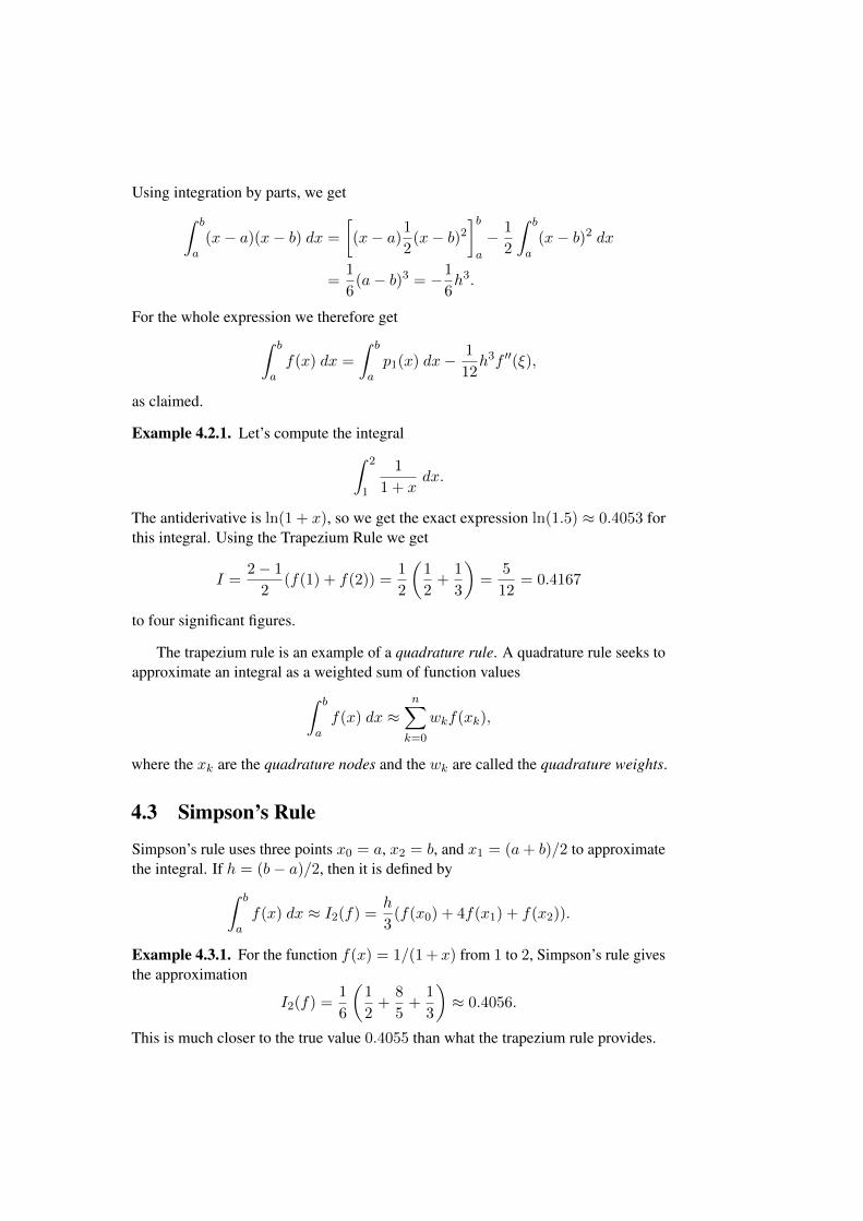
as claimed.

Example 4.2.1. Let’s compute the integral∫ 2

1

1

1 + xdx.

The antiderivative is ln(1 + x), so we get the exact expression ln(1.5) ≈ 0.4053 forthis integral. Using the Trapezium Rule we get

I =2− 1

2(f(1) + f(2)) =

1

2

(1

2+

1

3

)=

5

12= 0.4167

to four significant figures.

The trapezium rule is an example of a quadrature rule. A quadrature rule seeks toapproximate an integral as a weighted sum of function values∫ b

af(x) dx ≈

n∑k=0

wkf(xk),

where the xk are the quadrature nodes and the wk are called the quadrature weights.

4.3 Simpson’s Rule

Simpson’s rule uses three points x0 = a, x2 = b, and x1 = (a+ b)/2 to approximatethe integral. If h = (b− a)/2, then it is defined by∫ b

af(x) dx ≈ I2(f) =

h

3(f(x0) + 4f(x1) + f(x2)).

Example 4.3.1. For the function f(x) = 1/(1 + x) from 1 to 2, Simpson’s rule givesthe approximation

I2(f) =1

6

(1

2+

8

5+

1

3

)≈ 0.4056.

This is much closer to the true value 0.4055 than what the trapezium rule provides.

Example 4.3.2. For the function f(x) = 3x2 − x + 1 and interval 0, 1 (that is,h = 0.5), Simpson’s rule gives the approximation

I2(f) =1

6

(1 + 4(3

1

4− 1

2+ 1) + 3

)= 3/2.

The antiderivative of this polynomial is x3 − x2/2 + x, so the true integral is 1 −1/2 + 1 = 3/2. In this case, Simpson’s rule gives the exact value of the integral! Aswe will see, this is the case for any quadratic polynomial.

Simpson’s rule is a special case of a Newton-Cotes quadrature rule. A Newton-Cotes scheme of order n uses the Lagrange basis functions to construct the interpol-ation weights. Given nodes xk = a + kh, 0 ≤ k ≤ n, where h = (b − a)/n, theintegral is approximated by the integral of the Lagrange interpolant of degree n atthese points. If

pn =n∑k=0

Lkf(xk),

then ∫ b

af(x) dx ≈ In(f) :=

∫ b

apn(x) dx =

n∑k=0

wkf(xk),

where wk =∫ ba Lk(x) dx.

We now show that Simpson’s rule is indeed a Newton-Cotes rule of order 2. Letx0 = a, x2 = b and x1 = (a+b)/2. Define h := x1−x0 = (b−a)/2. The quadraticinterpolation polynomial is given by

p2 =(x− x1)(x− x2)

(x0 − x1)(x0 − x2)f(x0)+

(x− x0)(x− x2)(x1 − x0)(x1 − x2)

f(x1)+(x− x1)(x− x0)

(x2 − x0)(x2 − x1)f(x2).

We claim that

I2(f) =

∫ b

ap2(x) dx =

h

3(f(x0) + 4f(x1) + f(x2)).

To show this, we make use of the identities x1 = x0 + h, x2 = x0 + 2h, to get therepresentation (we use fi := f(xi))

p2 =f0

2h2(x− x1)(x− x2) +

f1−h2

(x− x0)(x− x2) +f2

2h2(x− x1)(x− x0).

Using integration by parts or otherwise, we can evaluate the integral∫ x2

x0

(x−x1)(x−x2) dx =2

3h3,

∫ x2

x0

(x−x0)(x−x2) dx = −4

3h3,

∫ x2

x0

(x−x0)(x−x1) dx =2

3h3.

Using this, we get ∫ x2

x0

p2 dx =h

3(f0 + 4f1 + f2).

This shows the claim. As with the Trapezium rule, we can bound the error forSimpson’s rule.

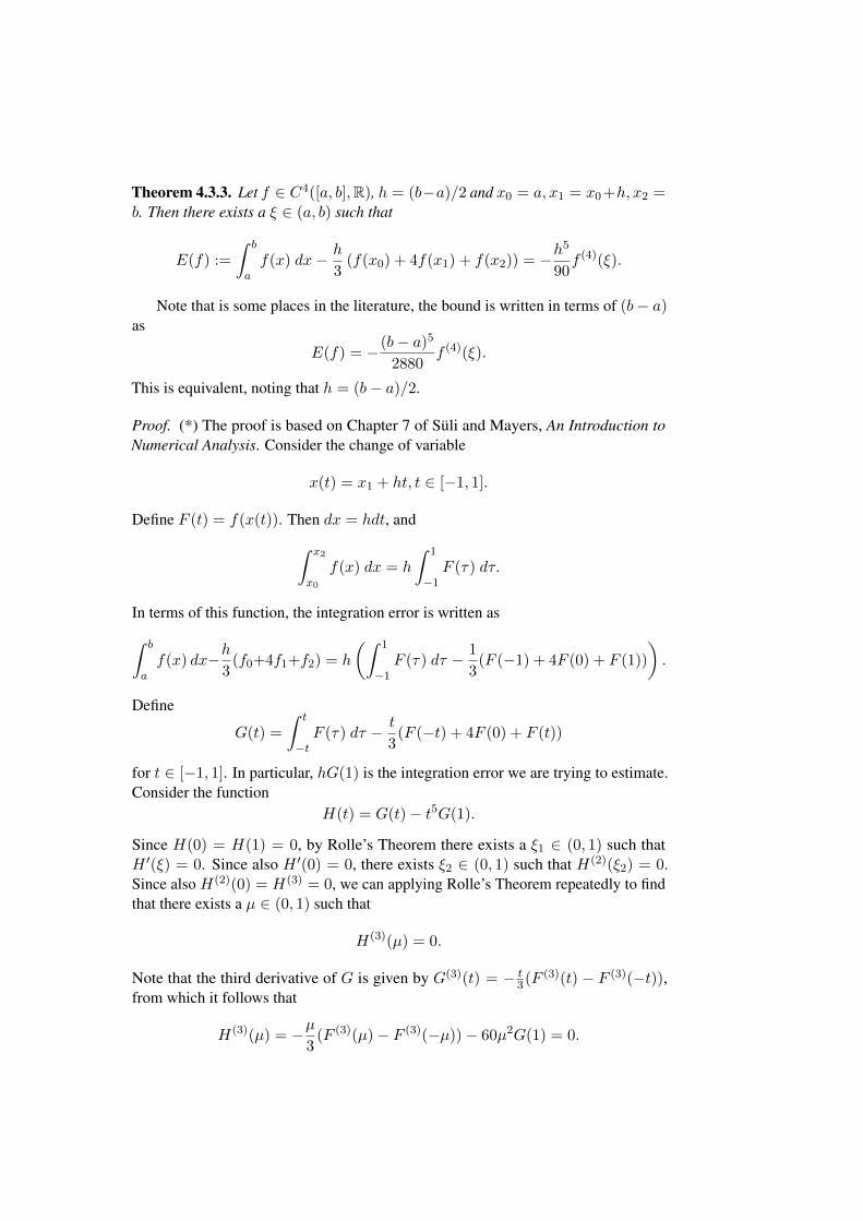
Theorem 4.3.3. Let f ∈ C4([a, b],R), h = (b−a)/2 and x0 = a, x1 = x0+h, x2 =b. Then there exists a ξ ∈ (a, b) such that

E(f) :=

∫ b

af(x) dx− h

3(f(x0) + 4f(x1) + f(x2)) = −h

5

90f (4)(ξ).

Note that is some places in the literature, the bound is written in terms of (b− a)as

E(f) = −(b− a)5

2880f (4)(ξ).

This is equivalent, noting that h = (b− a)/2.

Proof. (*) The proof is based on Chapter 7 of Süli and Mayers, An Introduction toNumerical Analysis. Consider the change of variable

x(t) = x1 + ht, t ∈ [−1, 1].

Define F (t) = f(x(t)). Then dx = hdt, and∫ x2

x0

f(x) dx = h

∫ 1

−1F (τ) dτ.

In terms of this function, the integration error is written as∫ b

af(x) dx−h

3(f0+4f1+f2) = h

(∫ 1

−1F (τ) dτ − 1

3(F (−1) + 4F (0) + F (1))

).

Define

G(t) =

∫ t

−tF (τ) dτ − t

3(F (−t) + 4F (0) + F (t))

for t ∈ [−1, 1]. In particular, hG(1) is the integration error we are trying to estimate.Consider the function

H(t) = G(t)− t5G(1).

Since H(0) = H(1) = 0, by Rolle’s Theorem there exists a ξ1 ∈ (0, 1) such thatH ′(ξ) = 0. Since also H ′(0) = 0, there exists ξ2 ∈ (0, 1) such that H(2)(ξ2) = 0.Since also H(2)(0) = H(3) = 0, we can applying Rolle’s Theorem repeatedly to findthat there exists a µ ∈ (0, 1) such that

H(3)(µ) = 0.

Note that the third derivative of G is given by G(3)(t) = − t3(F (3)(t) − F (3)(−t)),

from which it follows that

H(3)(µ) = −µ3

(F (3)(µ)− F (3)(−µ))− 60µ2G(1) = 0.

We can rewrite this equation as

−2

3µ2F (3)(µ)− F (3)(−µ)

(µ− (−µ)=

2

3µ290G(1).

Using that µ 6= 0, we can divide both sides by 2µ2/3. By the Mean Value Theoremthere exists a ξ ∈ (−µ, µ) such that

90G(1) = −F (4)(ξ),

from which we get for the error (after multiplying with h),

hG(1) = − h

90F (4)(ξ).

Now note that, using the substitution x = x1 + th we did at the beginning,

F (4)(t) =d4

dt4f(x) =

d4

dt4f(x1 + ht) = h4f (4)(x).

This finishes the (slightly tricky) proof.

From this derive the error bound

E2(f) =

∣∣∣∣∫ b

af(x) dx− I2(f)

∣∣∣∣ ≤ 1

90h5M4,

where M4 is an upper bound on the absolute value of the fourth derivative on theinterval [a, b].

0 0.2 0.4 0.6 0.8 10

0.1

0.2

0.3

0.4

0.5

0.6

0.7

0.8

0.9

1One step Trapezium Rule

0 0.2 0.4 0.6 0.8 10

0.1

0.2

0.3

0.4

0.5

0.6

0.7

0.8

0.9

1One step Simpson Rule

Week 5

5.1 The Runge phenomenon revisited

So far we have seen numerical integration methods that rely on linear interpolation(trapezium rule) and quadratic interpolation (Simpson’s rule), with error bounds:

E1(f) ≤ h3

12M2, E2(f) ≤ h5

90M4,

where E1(f) is the absolute error for the trapezium rule, E2(f) the absolute error forSimpson’s rule, h is the distance between two nodes, and Mk the maximum absolutevalue of the k-th derivative of f . In particular, it follows that the trapezium rule haserror 0 for polynomials of degree at most one, and Simpson’s rule for polynomials ofdegree at most three. One may wonder if increasing the degree of the interpolatingpolynomial decreases the integration error.

Example 5.1.1. Consider the infamous function

f(x) =1

1 + x2

on the interval [−5, 5]. Then integral of this function is given by∫ 5

−5

1

1 + x2dx = arctan(x)|5−5 = 2.7468.

Now let’s comptute the Newton-Cotes quadrature

In(f) =

∫ 5

−5pn(x) dx,

where pn(x) is the interpolation polynomial at n+ 1 equispaced points between −5and 5. The Figure 5.4 shows the absolute error for n from 1 to 15.

It turns out that in some cases (such as I12(f) = −0.31294), the numericalapproximation to the integral is negative, which is absurd. The reason is that some ofthe weights in the quadrature rule turn out to be negative.

As the example shows, increasing the degree may not always be a good choice,and we have to think of other ways to increase the precision of numerical integration.

29

0 5 10 15−1

0

1

2

3

4

5

6

7

8

0 5 10 150

1

2

3

4

5

6

Newton−CotesTrue value

Absolute error

Figure 5.4: Integration error for Newton-Cotes rules

5.2 Composite integration rules

The trapezium rule uses only two points to approximate an integral, certainly notenough for most applications. There are different ways to make use of more pointsand function values in order to increase precision. One way, as we have just seen withthe Newton-Cotes scheme and Simpson’s rule, is to use higher-order interpolants. Adifferent direction is to subdivide the interval into smaller intervals and use lower-orderschemes, like the trapezium rule, on these smaller intervals. For this, we subdividethe integral ∫ b

af(x) dx =

n−1∑j=0

∫ xj+1

xj

f(x) dx,

where x0 = a, xj = a + jh for 0 ≤ j ≤ n. The composite trapezium ruleapproximates each of these integrals using the trapezium rule:∫ b

af(x) dx ≈ h

2(f(x0) + f(x1)) +

h

2(f(x1) + f(x2)) + · · ·+ h

2(f(xn−1) + f(xn))

= h

(1

2f(x0) + f(x1) + · · · f(xn−1) +

1

2f(xn)

).

Example 5.2.1. Let’s look again at the function f(x) = 1/(1 + x) and apply thecomposite trapezium rule with h = 0.1 on the intervale [1, 2] (that is, with n = 10).Then ∫ 2

1

1

1 + xdx ≈ 0.1

(1

4+

1

2.1+ · · ·+ 1

2.9+

1

6

)= 0.4056.

Recall that the exact integral was 0.4055, and that Simpson’s rule also gaven anapproximation of 0.4056.

Theorem 5.2.2. If f ∈ C2(a, b) and a = x0 < · · · < xn = b, then there exists aµ ∈ (a, b) such that∫ b

af(x) dx = h

(1

2f(x0) + f(x1) + · · ·+ f(xn−1) +

1

2f(xn)

)− 1

12h2(b−a)f ′′(µ).

In particular, if M2 = maxa≤x≤b |f ′′(x)|, then the absolue error is bounded by

1

12h2(b− a)M2.

Proof. Recall from the error analysis of the trapezium rule that, for every j and someξj ∈ (xj , xj+1),

∫ b

af(x) dx =

n−1∑j=0

(h

2(f(xj) + f(xj+1))−

1

12h3f ′′(ξj)

)

= h ·(

1

2f(x0) + f(x1) + · · ·+ f(xn−1) +

1

2f(xn)

)− 1

12h3

n−1∑j=0

f ′′(ξj).

Clearly the values f ′′(ξj) lie between the minimum and maximum of f ′′ on theinterval (a, b), and so their average is also bounded by

minx∈[a,b]

f ′′(x) ≤ 1

n

n−1∑j=0

f ′′(ξj) ≤ maxx∈[a,b]

f ′′(x).

Since the function f ′′ is continuous on [a, b], it assumes every value between theminimum and the maximum, and in particular also the value given by the averageabove (this is the statement of the Intermediate Value Theorem). In other words, thereexists µ ∈ (a, b) such that the average above is attained:

1

n

n−1∑j=0

f ′′(ξj) = f ′′(µ).

Therefore we can write the error term as

− 1

12h3

n−1∑j=0

f ′′(ξj) = − 1

12h2(nh)f ′′(µ) = − 1

12h2(b− a)f ′′(µ),

where we used that h = (b− a)/n. This is the claimed expression for the error.

Example 5.2.3. Consider the function f(x) = e−x/x and the integral∫ 2

1

e−x

xdx.

What choice of parameter h will ensure that the approximation error of the compositetrapezium rule will by below 10−5? Let M2 denote an upper bound on the secondderivative of f(x). The approximation error for the composite trapezium rule withstep length h is bounded by

E(f) ≤ 1

12(b− a)h2 ·M2.

We can find out M2 by calculating the derivatives of f :

f ′(x) = −e−x(

1

x+

1

x2

)f ′′(x) = e−x

(1

x+

2

x2+

2

x3

).

The second derivative f ′′(x) has a maximum at x = 1, and the value is M2 ≈ 1.84.In the interval [1, 2] we therefore have the bound

E(f) ≤ 1

121.84h2(2− 1) = 0.1533h2.

If we choose, for example, h = 0.005 (this corresponds to taking n = 200 steps),then the error is bounded by 3.83 · 10−6.

To derive the composite version of Simpson’s rule, we subdivide the interval [a, b]into 2m intervals and set h = (b − a)/2m, xj = a + jh, 0 ≤ j ≤ 2m. Then, for1 ≤ j ≤ m, ∫ b

af(x) dx =

m∑j=1

∫ x2j

x2j−2

f(x) dx.

Applying Simpson’s rule to each of the integrals, we arrive at the expression

h

3(f(x0) + 4f(x1) + 2f(x2) + 4f(x3) + · · ·+ 4f(x2m−3) + 2f(x2m−2) + 4f(x2m−1) + f(x2m)) ,

where the coefficients of the f(xi) alternate between 4 and 2 for 1 ≤ i ≤ 2m − 1.Using an error analysis similar to the case of the composite trapezium rule, one obtainsan error bound

b− a180

h4M4,

where M4 is an upper bound on the absolute value of the fourth derivative of f on[a, b].

Example 5.2.4. Having an error of order h2 means that, every time we halve thestepsize (or, equivalently, double the number of points), the error decreases by a factorof 4. More precisely, for n = 2k we get an error E(f) ∼ 2−2k. Looking at theexample function f(x) = 1/(1 + x) and applying the composite Trapezium rule, weget the following relationship between the logarithm of the number of points log n andthe logarithm of the error. The fitted line has a slope of −1.9935 ≈ −2, as expectedfrom the theory.

0 1 2 3 4 5 6−20

−18

−16

−14

−12

−10

−8

−6

log of number of steps

log

of e

rror

Error for composite trapezium rule

Summarising, we have seen the following integration schemes with their corres-ponding error bounds:

Trapezium: 112(b− a)3M2

Composite Trapezium: 112h

2(b− a)M2

Simpson: 12880(b− a)5M4

Composite Simpson: 1180h

4(b− a)M4.

Note that we expressed the error bound for Simpson’s rule in terms of (b − a)rather than h = (b− a)/2. The h in the bounds for the composite rules correspondsto the distance between any two nodes, xj+1 − xj .

We conclude the section on chapter with a definition of the order of precision of aquadrature rule.

Definition 5.2.5. A quadrature rule I(f) has degree of precision k, if it evaluatespolynomials of degree at most k exactly. That is,

I(xj) =

∫ b

axj dx =

1

j + 1(bj+1 − aj+1), 0 ≤ j ≤ k.

For example, it is easy to show that the Trapezium rule has degree of precision 1(it evaluates 1 and x exactly), while Simpson’s rule has degree of precision 3 (ratherthan 2 as expected!). In general, Newton-Cotes quadrature of degree n has degree ofprecision n if n is odd, and n+ 1 if n is even.

Week 6

6.1 Numerical Linear Algebra

Problems in numerical analysis can often be formulated in terms of linear algebra.For example, the discretization of partial differential equations leads to problemsinvolving large systems of linear equations. The basic problem in linear algebra is tosolve a system of linear equations

Ax = b, (6.1.1)

where

A =

a11 · · · a1n...

. . ....

am1 · · · amn

is an m× n matrix with real numbers as entries, and

x =

x1...xn

, b =

b1...bm

are vectors. We will often deal with the case m = n.

There are two main classes of methods for solving such systems.

1. Direct methods attempt to solve (9.1.1) using a finite number of operations. Anexample is the well-known Gaussian elimination algorithm.

2. Iterative methods generate a sequence x0,x1, . . . of vectors in the hope that xk

converges (in a sense to be made precise) to a solution x of (9.1.1) as k →∞.

Direct methods generally work well for dense matrices and moderately large n.Iterative methods work well with sparse matrices, that is, matrices with very fewnon-zero entries aij , and large n.

Example 6.1.1. Consider the differential equation

−uxx = f(x)

35

with boundary conditions u(0) = u(1) = 0, where u is a twice differentiable functionon [0, 1], and uxx = ∂2u/∂x2 denotes the second derivative in x. We can discretizethe interval [0, 1] by setting ∆x = 1/(n+ 1), xj = j∆x, and

uj := u(xj), fj := f(xj).

The second derivative can be approximated by a finite difference

uxx ≈ui−1 − 2ui + ui+1

(∆x)2.

At any one point xj , the differential equation thus translates to

−ui−1 − 2ui + ui+1

(∆x)2= fj .

Making use of the initial conditions u(0) = u(1) = 0, we get the system of equations

− 1

(∆x)2

−2 1 0 0 · · · 0 01 −2 1 0 · · · 0 00 1 −2 1 · · · 0 0...

......

.... . .

......

0 0 0 0 · · · −2 10 0 0 0 · · · 1 −2

u1u2u3u4...

un−1un

=

f1f2f3...

fn−1fn

.

The matrix is very sparse, it has only 3n − 2 non-zero entries, out of n2 possible!This form is typical for matrices arising from partial differential equations, and iswell-suited for iterative methods that exploit the specific structure of the matrix.

6.2 The Jacobi and Gauss Seidel methods

In the following, we assume our matrices to be square (m = n). We will also use thefollowing bit of notation: upper indices are used to identify individual vectors in asequence of vectors, for example, x0,x1, . . . ,xi. Individual entries of a vector x aredenoted by xi, so, for example, the i-th entry of a k-th vectors would be written asx(k)i or simply xki .

A template for iteratively solving a linear system can be derived as follows. Writethe matrix A as a difference A = A1−A2, where A1 and A2 are somewhat “simpler”to handle than the original matrix. Then the system of equations Ax = b can bewritten as

A1x = A2x + b.

This motivates the following approach: start with a vector x0 and successively com-pute xk+1 from xk by solving the system

A1xk+1 = A2x

k + b. (6.2.1)

Note that at after the k-th step, the right-hand side is known, while the unknown to befound is the vector xk+1 on the left-hand side.

Jacobi’s Method

Decompose the matrix A as

A = L + D + U ,

where

L =

0 0 0 · · · 0 0a21 0 0 · · · 0 0a31 a32 0 · · · 0 0

......

.... . .

......

a(n−1)1 a(n−1)2 a(n−1)3 · · · 0 0

an1 an2 an3 · · · an(n−1) 0

, U =

0 a12 a13 · · · a1(n−1) a1n0 0 a23 · · · a2(n−1) a2n0 0 0 · · · a3(n−1) a3n...

......

. . ....

...0 0 0 · · · 0 a(n−1)n0 0 0 · · · 0 0

are the lower and upper triangular parts, and

D = diag(a11, . . . , ann) :=

a11 0 · · · 00 a22 · · · 0...

.... . .

...0 0 · · · ann

is the diagonal part. Jacobi’s method chooses A1 = D and A2 = −(L + U). Thecorresponding iteration (9.1.2) then looks like Dxk+1 = −(L + U)xk + b. Oncewe know xk, this is a particularly simple system of equations: the matrix on the left isdiagonal! Solving for xk+1,

xk+1 = D−1(b− (L + U)xk). (6.2.2)

Note that since D is diagonal, it is easy to invert: just invert the individual entries.

Example 6.2.1. For a concrete example, take the following matrix with its decom-position in diagonal and off-diagonal part:

A =

(2 −1−1 2

)=

(2 00 2

)+

(0 −1−1 0

).

Since (2 00 2

)−1=

(1/2 00 1/2

)=

1

2

(1 00 1

),

we get the iteration scheme

xk+1 =

(0 1/2

1/2 0

)xk +

1

2b.

We can also write the iteration (6.2.2) in terms of individual entries. If we denote

xk :=

x(k)1...

x(k)n

,

i.e., we write x(k)i for the i-th entry of the k-th iterate, then the iteration (6.2.2)becomes

x(k+1)i =

1

a11

bi −∑j 6=i

aijx(k)j

. (6.2.3)

for 1 ≤ i ≤ n.Let’s try this out with b = (1, 1)>, to see if we get a solution. Let x0 = 0 to start

with. Then

x1 =

(0 1/2

1/2 0

)0 +

(1212

)=

(1212

)x2 =

(0 1/2

1/2 0

)x1 +

(1212

)=

(0 1/2

1/2 0

)(1212

)+

(1212

)=

(3434

)x3 =

(0 1/2

1/2 0

)x2 +

(1212

)=

(0 1/2

1/2 0

)(3434

)+

(1212

)=

(7878

)We see a pattern emerging: in fact, one can show (do this!) that in this example,

xk =

(1− 2−k

1− 2−k

).

In particular, as k →∞ the vectors xk approach (1, 1)>, which is easily verified tobe a solution of Ax = b.

Week 7

We saw that a general approach to finding an approximate solution to a system oflinear equations

Ax = b

is to generate a sequence of vectors x(k) for k ≥ 0 by some procedure

x(k+1) = Tx(k) + c,

in the hope that the sequence approaches a solution. In the case of the Jacobi method,we had the iteration

x(k+1) = D−1(b− (L + U)x(k)),

with L,D and U the lower, diagonal, and upper triangular part of A. That is,

T = −D−1(L + U), c = D−1b.

Next, we discuss a refinedment of this method and will also address the issue ofconvergence.

Gauss-Seidel

In the Gauss-Seidel method, we use a different decomposition, leading to the followingsystem

(D + L)xk+1 = −Uxk + b. (7.0.1)

Though the right-hand side is not diagonal, as in the Jacobi method, the system is stilleasily solved for xk+1 when xk is given. To derive the entry-wise formula for thismethod, we take a closer look at (7.0.1)

a11 0 · · · 0a21 a22 · · · 0

......

. . ....

an1 an2 · · · ann

x(k+1)1

x(k+1)2

...x(k+1)n

=

b1b2...bn

−

0 a12 · · · a1n0 0 · · · a2n...

.... . .

...0 0 · · · 0

x(k)1

x(k)2...

x(k)n

.

39

Writing out the equations, we get

a11x(k+1)1 = b1 −

(a12x

(k)2 + · · ·+ a1nx

(k)n

)a21x

(k+1)1 + a22x

(k+1)2 = b2 −

(a23x

(k)3 + · · ·+ a2nx

(k)n

)...

ai1x(k+1)1 + · · ·+ aiix

(k+1)i = bi −

(aii+1x

(k)i+1 + · · ·+ ainx

(k)n

)Rearranging this, we get the formula

x(k+1)i =

1

aii

bi −∑j<i

aijx(k+1)j −

∑j>i

aijx(k)j

for the k + 1-th iterate of xi. Note that in order to compute the k + 1-th iterate of xi,we already use values of the k + 1-th iterate of xj for j < i. Note how this differsfrom the Jacobi form, where we only resort to the k-th iterate. Both methods havetheir advantages and disadvantages. While Gauss-Seidel may require less storage(we can overwrite each x(k)i by x(k+1)

i as we don’t need the old value subsequently),Jacobi’s method can be used easier in parallel (that is, all the x(k+1)

i can be computedby different processors for each i).

Example 7.0.1. Consider a simple system of the form 2 −1 0−1 2 −10 −1 2

x =

111

.

Note that this is the kind of system that arises in the discretisation of a partial dif-ferential equation. Although for matrices of this size we can easily solve the systemdirectly, we will illustrate the use of the Gauss-Seidel method. The Gauss-Seideliteration has the form 2 0 0

−1 2 00 −1 2

xk+1 =

0 −1 00 0 −10 0 0

xk +

111

If we choose the starting point x0 = (0, 0, 0), then 2 0 0

−1 2 00 −1 2

x1 =

0 1 00 0 10 0 0

x0 +

111

=

111

The system is easily solved to find x1 = (1/2, 3/4, 7/8)>. Continuing this processwe get x2,x3, ... until we are satisfied with the accuracy of the solution. Alternatively,we can also solve the system using the coordinate-wise interpretation.

7.1 Vector Norms

We have seen in previous examples that the sequence of vectors xk generated bythe Jacobi method “approaches” the solution of the system of equations A as wekeep going. In order to make this type of convergence precise, we need to be able tomeasure distances between vectors and matrices.

Definition 7.1.1. A vector norm on Rn is a real-valued function ‖·‖ that satisfies thefollowing conditions:

1. For all x ∈ Rn: ‖x‖ ≥ 0 and ‖x‖ = 0 if and only if x = 0.

2. For all α ∈ R: ‖αx‖ = |α|‖x‖.

3. For x,y ∈ Rn: ‖x + y‖ ≤ ‖x‖+ ‖y‖ (Triangle Inequality).

Example 7.1.2. The typical examples are the following:

1. The 2-norm

‖x‖2 =

√√√√ n∑i=1

x2i =(x>x

)1/2.

This is just the usual notion of Euclidean length.

2. The 1-norm

‖x‖1 =n∑i=1

|xi|.

3. The∞-norm‖x‖∞ = max

1≤i≤n|xi|.

A convenient way to visualise these norms is via their “unit circles”. If we look at thesets

{x ∈ R2 : ‖x‖p = 1}

for p = 2, 1,∞, then we get the following shapes:

Now that we have defined a way of measuring distances between vectors, we cantalk about convergence.

Definition 7.1.3. A sequence of vectors xk ∈ Rn, k = 0, 1, 2, . . . , converges tox ∈ Rn with respect to a norm ‖·‖, if for all ε > 0 there exists an N > 0 such thatfor all k ≥ N :

‖xk − x‖ < ε.

In words: we can get arbitrary close to x by choosing k sufficiently large.

We sometimes write

limk→∞

xk = x or xk → x

to indicate that a sequence x0,x1, . . . converges to a vector x. If we want to indicatethe norm with respect to which convergence is measured, we sometimes write

xk →1x, xk →

∞x, xk →

2x

to indicate convergence with respect to the 1-,∞-, and 2-norms, respectively.The following lemma implies that for the purpose of convergence, it doesn’t matter

whether we take the∞- or the 2-norm.

Lemma 7.1.4. For x ∈ Rn,

‖x‖∞ ≤ ‖x‖2 ≤√n‖x‖∞.

Proof. Let M := ‖x‖∞ = max1≤i≤n |xi|. Note that

‖x‖2 = M ·

(n∑i=1

x2iM2

) 12

≤M√n = ‖x‖∞

√n,

because x2i /M2 ≤ 1 for all i. This shows the second inequality. For the first one, note

that there is an i such that M = |xi|. It follows that

‖x‖2 = M ·

(n∑i=1

x2iM2

) 12

≥M = ‖x‖∞.

This completes the proof.

A similar relationship can be shown between the 1-norm and the 2-norm, and alsobetween the 1-norm and the∞-norm.

Corollary 7.1.5. Convergence in the 2-norm is equivalent to convergence in the∞-norm:

xk →2x ⇐⇒ xk →

∞x.

In words: if xk → x with respect to the∞-norm, then xk → x with respect to the2-norm, and vice versa.

Proof. Assume that xk → x with respect to the 2-norm and let ε > 0. Since xk

converges with respect to the 2-norm, there exists N > 0 such that for all k > N ,‖xk − x‖2 < ε. Since ‖xk − x‖∞ ≤ ‖xk − x‖2, we also get convergence withrespect to the ∞-norm. Now assume conversely that xk converges with respectto the ∞-norm. Then given ε > 0, for ε′ = ε/

√n there exists N > 0 such that

‖xk − x‖∞ < ε′ for k > N . But since ‖xk − x‖2 ≤√n‖xk − x‖∞ <

√nε′ = ε,

it follows that xk also converges with respect to the 2-norm.

The benefit of this type of result is that some norms are easier to compute thanothers. Even if we are interested in measuring convergence with respect to the 2-norm,it may be easier to show that a sequence converges with respect to the∞-norm, andonce this is shown, convergence in the 2-norm follows automatically by the abovecorollary.

Example 7.1.6. Let’s look at the vector

x =

1−11

.

The different norms are ‖x‖2 =√

3, ‖x‖1 = 3, ‖x‖∞ = 1.

Week 8

Recall that we introduced vector norms ‖x‖ as a way of measuring convergence of asequence of vectors x(0),x(1), . . . . One important property of such norms is that theycan be related to each other, as the following lemma shows.

Lemma 8.0.1. For x ∈ Rn,

‖x‖∞ ≤ ‖x‖2 ≤√n‖x‖∞.

Proof. Let M := ‖x‖∞ = max1≤i≤n |xi|. Note that

‖x‖2 = M ·

(n∑i=1

x2iM2

) 12

≤M√n = ‖x‖∞

√n,

because x2i /M2 ≤ 1 for all i. This shows the second inequality. For the first one, note

that there is an i such that M = |xi|. It follows that

‖x‖2 = M ·

(n∑i=1

x2iM2

) 12

≥M = ‖x‖∞.

This completes the proof.

A similar relationship can be shown between the 1-norm and the 2-norm, and alsobetween the 1-norm and the∞-norm. The importance of such a result is that whenshowing convergence of a sequence, it does not matter which norm we use!

Corollary 8.0.2. Convergence in the 2-norm is equivalent to convergence in the∞-norm:

xk →2x ⇐⇒ xk →

∞x.

In words: if xk → x with respect to the∞-norm, then xk → x with respect to the2-norm, and vice versa.

Proof. Assume that xk → x with respect to the 2-norm and let ε > 0. Since xk

converges with respect to the 2-norm, there exists N > 0 such that for all k > N ,‖xk − x‖2 < ε. Since ‖xk − x‖∞ ≤ ‖xk − x‖2, we also get convergence with

45

respect to the ∞-norm. Now assume conversely that xk converges with respectto the ∞-norm. Then given ε > 0, for ε′ = ε/

√n there exists N > 0 such that

‖xk − x‖∞ < ε′ for k > N . But since ‖xk − x‖2 ≤√n‖xk − x‖∞ <

√nε′ = ε,

it follows that xk also converges with respect to the 2-norm.

The benefit of this type of result is that some norms are easier to compute thanothers. Even if we are only interested in measuring convergence with respect tothe 2-norm, it may be easier to show that a sequence converges with respect to the∞-norm, and once this is shown, convergence in the 2-norm follows automatically bythe above corollary.

8.1 Matrix norms

To study the convergence of iterative methods we also need norms for matrices. Recallthat the Jacobi and Gauss-Seidel methods generate a sequence xk of vectors by therule

xk+1 = Txk + c

for some matrix T . The hope is that this sequence will converge to a vector x suchthat x = Tx + c. Given such an x, we can subtract x from both sides of the iterationto obtain

xk+1 − x = Txk + c− x = T (xk − x).

That is, the difference xk+1 − x arises from the previous difference xk − x bymultiplication with T . For convergence we want ‖xk − x‖ to become smaller as kincreases, or in other words, we want multiplication with T to reduce the norm of avector. In order to quantify the effect of a linear transformation T on the norm of avector, we introduce the concept of a matrix norm.

Definition 8.1.1. A matrix norm is a non-negative function ‖·‖ on the set of real n×nmatrices such that, for every n× n matrix A,

1. ‖A‖ ≥ 0 and A = 0 if and only if A = 0.

2. For all α ∈ R, ‖αA‖ = |α|‖A‖.

3. For all n× n matrices A,B: ‖A + B‖ ≤ ‖A‖+ ‖B‖.

4. For all n× n matrices A,B: ‖AB‖ ≤ ‖A‖‖B‖.

Note that parts 1-3 just state that a matrix norm also is a vector norm, if we thinkof the matrix as a vector. Part 4 of the definition has to do with the “matrix-ness” of amatrix. The most useful class of matrix norms are the operator norms induced by avector norm.

Example 8.1.2. If we treat a matrix as a big vector, then the 2-norm is called theFrobenius norm of the matrix,

‖A‖F =

√√√√ n∑i,j=1

a2ij .

The properties 1-3 are clearly satisfied, since this is just the 2-norm of the matrixconsidered as a vector. Property 4 can be verified using the Cauchy-Schwarz inequality,and is left as an exercise.

The most important matrix norms are the operator norms associated to certainvector norms, which measure the extent by which a vector x is “stretched” by thematrix A with respect to a given norm.

Definition 8.1.3. Given a vector norm ‖·‖, the corresponding operator norm of ann× n matrix A is defined as

‖A‖ = maxx6=0

‖Ax‖‖x‖

= maxx∈Rn‖x‖=1

‖Ax‖.

Remark 8.1.4. To see the second inequality, note that for x 6= 0 we can write

‖Ax‖‖x‖

= ‖A x

‖x‖‖ = ‖Ay‖,

with y = x/‖x‖, where we used Property (2) of the definition of a vector norm. Thevector y = x/‖x‖ is a vector with norm ‖y‖ = ‖x/‖x‖‖ = 1, so that for everyx 6= 0 there exists a vector y with ‖y‖ = 1 such that

‖Ax‖‖x‖

= ‖Ay‖.

In particular, minimizing the left-hand side over x 6= 0 give the same result asminimizing the right-hand side over y with ‖y‖ = 1.

First, we have to verify that the operator norm is indeed a matrix norm.

Theorem 8.1.5. The operator norm corresponding to a vector norm ‖·‖ is a matrixnorm.

Proof. Properties 1-3 are easy to verify from the corresponding properties of thevector norms. For example, ‖A‖ ≥ 0 because by the definition, there is no way itcould be negative. To show the property 4, namely,

‖AB‖ ≤ ‖A‖‖B‖

for n× n matrices A and B, we first note that for any y ∈ Rn,

‖Ay‖‖y‖

≤ maxx6=0

‖Ax‖‖x‖

= ‖A‖,

and therefore‖Ay‖ ≤ ‖A‖‖y‖.

Now let y = Bx for some x with ‖x‖ = 1. Then

‖ABx‖ ≤ ‖A‖‖Bx‖ ≤ ‖A‖‖B‖.

As this inequality holds for all unit-norm x, it also holds for the vector that maximises‖ABx‖, and therefore we get

‖AB‖ = max‖x‖=1

‖ABx‖ ≤ ‖A‖‖B‖.

This completes the proof.

Example 8.1.6. Consider the matrix

A =

(2 11 2

).

The matrix norm ‖A‖2 gives the maximum length ‖Ax‖2 among all x with ‖x‖2 = 1.If we draw the circle C = {x : ‖x‖2 = 1} and the ellipse E = {Ax : ‖x‖2 = 1},then ‖A‖2 is the length of the longest axis of the ellipse.

x

Ax

Even though the operator norms with respect to the various vector norms are ofimmense importance in the analysis of numerical methods, they are hard to computeor even estimate from their definition alone. It is therefore useful to have alternativecharacterisations of these norms. The first of these characterisations is concerned withthe norms ‖·‖1 and ‖·‖∞, and provides an easy criterion to compute these.

Lemma 8.1.7. For an n×n matrix A, the operator norms with respect to the 1-normand the∞-norm are given by

‖A‖1 = max1≤j≤n

n∑i=1

|aij | (maximum absolute column sum) ,

‖A‖∞ = max1≤i≤n

n∑j=1

|aij | (maximum absolute row sum) .

Proof. (*) We will proof this for the∞-norm. We first show the inequality ‖A‖∞ ≤max1≤i≤n

∑nj=1 |aij |. Let x be a vector such that ‖x‖∞ = 1. That means that all

the entries have absolute value |xi| ≤ 1. It follows that

‖Ax‖∞ = max1≤i≤n

∣∣∣∣∣∣n∑j=1

aijxj

∣∣∣∣∣∣≤ max

1≤i≤n

n∑j=1

|aijxj |

≤ max1≤i≤n

n∑j=1

|aij |,

where the inequality follows from writing out the matrix vector product, interpretingthe ∞-norm, using the triangle inequality for the absolute value, and the fact that|xj | ≤ 1 for 1 ≤ j ≤ n. Since this holds for arbitrary x with ‖x‖∞ = 1, it also holdsfor the vector that maximises max‖x‖∞=1 ‖Ax‖∞ = ‖A‖∞, which concludes theproof of one directions.

In order to show ‖A‖∞ ≥ max1≤i≤n∑n

j=1 |aij |, let i be the index at which themaximum of the sum is attained:

max1≤i≤n

n∑j=1

|aij | =n∑j=1

|aij |.

Choose y to be the vector with entries yj = 1 if aij > 0 and yj = −1 if aij < 0. Thisvector satisfies ‖y‖∞ = 1 and, moreover,

n∑j=1

yjaij =

n∑j=1

|aij |,

by the choice of the yj . We therefore have

‖A‖∞ = max‖x‖∞=1

‖Ax‖∞ ≥ ‖Ay‖∞ =n∑j=1

|aij | = max1≤i≤n

n∑j=1

|aij |.

This finishes the proof.

Example 8.1.8. Consider the matrix

A =

−7 3 −12 4 5−4 6 0

.

The operator norms with respect to the 1- and∞-norm are

‖A‖1 = max{13, 13, 6} = 13, ‖A‖∞ = max{11, 11, 10} = 11.

How do we characterise the matrix 2-norm ‖A‖2 of a matrix? The answer isin terms of the eigenvalues of A. Recall that a (possibly complex) number λ is aneigenvalue of A, with associated eigenvector u, if

Au = λu.

Definition 8.1.9. The spectral radius of A is defined as

ρ(A) = max{|λ| : λ eigenvalue of A}.

Theorem 8.1.10. For an n× n matrix A we have

‖A‖2 =√ρ(A>A).

Proof. (*) Note that for a vector x, ‖Ax‖22 = x>A>Ax. We can therefore expressthe squared 2-norm of A as

‖A‖22 = max‖x‖2=1

‖Ax‖22 = max‖x‖2=1

x>A>Ax.

As a continuous function over a compact set, f(x) = x>A>Ax attains a uniquemaximum u on the unit sphere {x : ‖x‖2 = 1}. By the Lagrange multiplier theorem(see the appendix), there exist a parameter λ such that

∇f(u) = λ2u. (8.1.1)

To compute the gradient∇f(x), set B = A>A, so that

f(x) = x>Bx =n∑

i,j=1

bijxixj =n∑i=1

biix2i + 2

∑i<j

bijxixj ,

where the last inequality follows from the symmetry of B (that is, bij = bji). Then

∂f

∂xk= 2bkkxk + 2

∑i 6=k

bkixi = 2

n∑i=1

bkixi.

But this expression is just the two times the k-th row of Bx, so that

∇f(x) = 2Bx = 2A>Ax.

Using this in Equation (10.2.1), we find

A>Au = λu,

so that λ is an eigenvalue of A>A. Using that u>u = ‖u‖2 = 1, we also have

u>A>Au = λu>u = λ,

and since u was a maximiser of the left-hand function, it follows that λ is the maximaleigenvalue of A>A, λ = ρ(A>A). Summarising, we have ‖A‖22 = ρ(A>A), whatwas to be shown.

Example 8.1.11. Let

A =

1 0 20 1 −1−1 1 1

.

The eigenvalues are the roots of the characteristic polynomial

p(λ) = det(A− λ1) = det

1− λ 0 20 1− λ −1−1 1 1− λ

.

Evaluating this determinant, we get the equation

(1− λ)(λ2 − 2λ+ 4) = 0.

The solutions are given by λ1 = 1 and λ2,3 = 1±√

3i. The spectral radius of A istherefore

ρ(A) = max{1, 2, 2} = 2.

Week 9

We introduced the spectral radius of a matrix, ρ(A), as the maximum absolute valueof an eigenvalue of A, and characterized the 2-norm of A as

‖A‖2 =√ρ(A>A).

Note that the matrix A>A is symmetric, and therefore has real eigenvalues.For symmetric matrices A, that is, matrices such that A> = A, the situation is

simpler: the 2-norm is just the spectral radius.

Lemma 9.0.1. If A is symmetric, then ‖A‖2 = ρ(A).

Proof. Let λ be an eigenvalue of A with corresponding eigenvector u, so that

Au = λu.

ThenA>Au = A>λu = λA>u = λAu = λ2u.

It follows that λ2 is eigenvalue of A>A with corresponding eigenvector u. Inparticular,

‖A‖22 = ρ(A>A) = max{λ2 : λ eigenvalue of A} = ρ(A)2.

Taking square roots on both sides, the claim follows.

Example 9.0.2. We compute the eigenvalues, and thus the spectral radius and the2-norm, of the finite difference matrix

A =

2 −1 0 0 · · · 0 0−1 2 −1 0 · · · 0 00 −1 2 −1 · · · 0 0...

......

.... . .

......

0 0 0 0 · · · 2 −10 0 0 0 · · · −1 2

.

53

Let h = 1/(n+ 1). We first claim that the vectors uk, 1 ≤ k ≤ n, defined by

uk =

sin(kπh)...

sin(nkπh)

are the eigenvectors of A, with corresponding eigenvalues

λk = 2(1− cos(kπh)).

This can be verified by checking that

Auk = λkuk.

In fact, for 2 ≤ k ≤ n− 1, the left-hand side of the j-th entry of the above product isgiven by

2 sin(jkπh)− sin((j − 1)kπh)− sin((j + 1)kπh).

Using the trigonometric identity sin(x+ y) = sin(x) cos(y) + cos(x) sin(y), we canwrite this as

2 sin(jkπh)− (cos(kπh) sin(jkπh)− cos(jkπh) sin(kπh))

− (cos(kπh) sin(jkπh) + cos(jkπh) sin(kπh))

= 2(1− cos(kπh)) · sin(jkπh).

Now sin(jkπh) is just the j-th entry of uk as defined above, so the coefficient infront must equal the corresponding eigenvalue. The argument for k = 1 and k = n issimilar.

The spectral radius is the maximum modulus of such an eigenvalue,

ρ(A) = max1≤k≤n

|λk| = 2

(1− cos

(nπ

n+ 1

)).

As the matrix A is symmetric, this is also equal to the matrix 2-norm A:

‖A‖2 = 2

(1− cos

(nπ

n+ 1

)).

9.1 Convergence of Iterative Algorithms

In this section we focus on algorithms that attempt to solve a system of equations

Ax = b (9.1.1)

by starting with some vector x0 and then successively computing a sequence xk,k ≥ 1, by means of a rule

xk+1 = Txk + c (9.1.2)

for some matrix T and vector c. The hope is that the resulting sequence will convergeto a solution x of Ax = b.

Example 9.1.1. The Jacobi and Gauss-Seidel methods fall into this framework. Recallthe decomposition

A = L + D + U ,

where L is the lower triangular, D the diagonal and U the upper triangular part. Thenthe Jacobi method corresponds to the choice

T = TJ = −D−1(L + U), c = D−1b,

while the Gauss-Seidel method corresponds to

T = TGS = −(L + D)−1U , c = (L + D)−1b,

Lemma 9.1.2. Let T and c be the matrices in the iteration scheme (9.1.2) corres-ponding to either the Jacobi method or the Gauss-Seidel method, and assume that Dand L + D are invertible. Then x is a solution of the system of equations (9.1.1) ifand only if x is a fixed point of the iteration (9.1.2), that is,

x = Tx + c.

Proof. We write down the proof for the case of Jacobi’s method, the Gauss-Seidelcase being similar. We have

Ax = b⇔ (L + D + U)x = b

⇔Dx = −(L + U)x + b

⇔ x = −D−1(L + U)x + D−1b

⇔ x = Tx + c.

This shows the claim.

The problem of solving Ax = b is thus reduced to the problem of finding a fixedpoint to an iteration scheme. The following important result shows how to bound thedistance of an iterate xk from the solution x in terms of the operator norm of T andan initial distance of x0.

Theorem 9.1.3. Let x be a solution of Ax = b, and xk, k ≥ 0, be a sequence ofvectors such that

xk+1 = Txk + c

for an n × n matrix T and a vector c ∈ Rn. Then, for any vector norm ‖·‖ andassociated matrix norm, we have

‖xk+1 − x‖ ≤ ‖T ‖k+1‖x0 − x‖.

for all k ≥ 0.

Proof. We proof this by induction on k. Recall that for every vector x, we have

‖Tx‖ ≤ ‖T ‖‖x‖.

Subtracting the identity x = Tx+ c from xk+1 = Txk + c and taking norms we get

‖xk+1 − x‖ = ‖T (xk − x)‖ ≤ ‖T ‖‖xk − x‖. (9.1.3)

Setting k = 0 gives the claim of the theorem for this case. If we assume that the claimholds for k − 1, k ≥ 1, then

‖xk − x‖ ≤ ‖T‖k‖xk−1 − x‖

by this assumption, and plugging this into (9.1.3) finishes the proof.

Corollary 9.1.4. Assume that in addition to the assumptions of Theorem 9.1.3, wehave ‖T ‖ < 1. Then the sequence xk, k ≥ 0, converges to a fixed point x withx = Tx + c with respect to the chosen norm ‖·‖.

Proof. Assume x0 6= x (otherwise there is nothing to prove) and let ε > 0. Since‖T ‖ < 1, ‖T ‖k → 0 as k → ∞. In particular, there exists an integer N > 1 suchthat for all k > N ,

‖T ‖k < ε

‖x0 − x‖.

It follows that for k > N we have ‖xk − x‖ < ε, which completes the convergenceproof.

Recall that for the Gauss-Seidel and Jacobi methods, a fixed point of Tx + cwas the same as a solution of Ax = b. It follows that the Gauss-Seidel and Jacobimethods converge to a solution (with respect to some norm) provided that ‖T ‖ < 1.Note also that either one of ‖T ‖∞ < 1 or ‖T ‖2 < 1 will imply convergence withrespect to both the 2-norm and the∞-norm. The reason is the equivalence of norms

‖x‖∞ ≤ ‖x‖2 ≤√n‖x‖∞,

which implies that if the sequence xk, k ≥ 0, converges to x with respect to one ofthese norms, it also converges with respect to the other one. Such an equivalence canalso be shown between the 2- and the 1-norm.

So far we have seen that the condition ‖T ‖ < 1 ensures that an iterative schemeof the form (9.1.2) converges to a vector x such that x = Tx + c as k → ∞. Theconverse is not true, there are examples for which ‖T ‖ ≥ 1 but the iteration (9.1.2)converges nevertheless.

Example 9.1.5. Recall the finite difference matrix

A =

2 −1 0 · · · 0−1 2 −1 · · · 00 −1 2 · · · 0...

......

. . ....

0 0 0 · · · 2

and apply the Jacobi method to compute a solution of Ax = b. The Jacobi methodcomputes the sequence xk+1 = Txk + c, where c = 1

2b and

T = TJ = −D−1(L + U) =1

2

0 1 0 · · · 01 0 1 · · · 00 1 0 · · · 0...

......

. . ....

0 0 0 · · · 0

.

We have ‖T ‖∞ = 1, so the convergence criterion doesn’t apply for this norm.However, one can show that all the eigenvalues satisfy |λ| < 1. Since the matrix T issymmetric, we have

‖T ‖2 = ρ(T ) < 1,

where ρ(T ) denotes the spectral radius. It follows that the iteration (9.1.2) doesconverge with respect to the 2-norm, and therefore also with respect to the∞-norm,despite having ‖T‖∞ = 1.

It turns out that the spectral radius gives rise to a necessary and sufficient conditionfor convergence.

Theorem 9.1.6. The iterates xk of (9.1.2) converge to a solution x of x = Tx + cfor all starting points x0 if and only if ρ(T ) < 1.

Proof. (*) Let x0 be any starting point, and define, for all k ≥ 0,

zk = xk − x.

Then zk+1 = Tzk, as is easily verified. The convergence of the sequence xk to x isthen equivalent to the convergence of zk to 0.

Assume T has n eigenvalues λk (possibly 0), 1 ≤ k ≤ n. We will only prove theclaim for case where the eigenvectors uk form a basis of Rn (equivalently, that T isdiagonalisable), and mention below how the general case can be deduced. We canwrite

z0 =n∑j=1

αjuj (9.1.4)

for some coefficients αj . For the iterate we get

zk+1 = Tzk

= T k+1z0

= T k+1

n∑j=1

αjuj

=

n∑j=1

αjTk+1uj

=n∑j=1

αjλk+1j uj .

Now assume ρ(T ) < 1. Then |λj | < 1 for all eigenvalues λj , and therefore λk+1j → 0

as k → ∞. Therefore, zk+1 → 0 as k → ∞ and xk+1 → x. If, on the other hand,ρ(T ) ≥ 1, then there exists an index j such that |λj | ≥ 1. If we choose a startingpoint x0 such that the coefficient αj in (9.1.4) is not zero, then |αjλk+1

j | ≥ |αj | forall k and we deduce that zk+1 does not converge to zero.

If T is not diagonalisable, then we still have the Jordan normal form J = P−1TP ,where P is an invertible matrix and J consists of Jordan blocks

λi 1 · · · 00 λi · · · 0...

.... . .

...0 0 · · · λi

on the diagonal for each eigenvalue λi. Rather than considering a basis of eigenvectors,we take one consisting of generalized eigenvectors, that is, solutions to the equation

(A− λi1)k = 0,

where k <= m and m is the geometric multiplicity of λi.

9.2 Gershgorin’s circles

So far we have seen that an iterative method xk+1 = Txk + c converges to a fixedpoint x = Tx + c if and only if the spectral radius ρ(T ) < 1. Since the eigenvaluesare in general not easy to compute, the question is whether there is a convenientway to estimate ρ(T ). One way to bound the size of the eigenvalues is by meansof Gershgorin’s Theorem. Recall that eigenvalues of a matrix A can be complexnumbers.

Theorem 9.2.1. Every eigenvalue of an n × n matrix A lives in one of the circlesC1, . . . , Cn, where Ci has centre at the diagonal aii and radius

ri =∑j 6=i|aij |.

Example 9.2.2. Consider the matrix

A =

2 −1 0−1 4 −10 −1 8

.

The centres are given by 2, 4, 8, and the radii by r1 = 1, r2 = 2, r3 = 1.

Figure 9.5: Gershgorin’s circles.

Proof. Let λ be an eigenvalue of A, with associated eigenvector u, so that

Au = λu.

The i-th row of this equation looks like

λui =n∑j=1

aijuj .

Bringing aii to the left, this implies the inequality

|λ− aii| ≤∑j 6=i|aij ||uj ||ui|

.

If the index i is such that ui is the component of u with largest absolute value, thenthe right-hand side is bounded by ri, and we get

|λ− aii| ≤ ri,

which implies that λ lies in a circle of radius ri around aii.

Gershgorin’s Theorem has implications on the convergence of Jacobi’s method.To state these implications, we need a definition.

Definition 9.2.3. A matrix A is called diagonally dominant, if for all indices i wehave

|aii| > ri.

Corollary 9.2.4. Let A be diagonally dominant. Then the Jacobi method convergesto a solution of the system Ax = b for any starting point x0.

Proof. We need to show that if A is diagonally dominant, then ρ(TJ) < 1, whereTJ = −D−1(L + U) is the iteration matrix of Jacobi’s method. The i-th row of TJis

− 1

aii

(ai1 · · · aii−1 0 aii+1 · · · ain

).

By Gershgorin’s Theorem, all the eigenvalues of TJ lie in a circle around 0 of radius

ri =1

|aii|∑j 6=i|aij |.

It follows that if A is diagonally dominant, then ri < 1, and therefore |λ| < 1 for alleigenvalues λ of TJ . In particular, ρ(TJ) < 1 and Jacobi’s method converges for anyx0.

Week 10

10.1 The Condition Number

In this section we discuss the sensitivity of a system of equations Ax = b to perturba-tions in the data. This sensitivity is quantified by the notion of condition number. Webegin by illustrating the problem with a small example.

Example 10.1.1. Let’s look at the system of equations with

A =

(ε 10 1

), b =

(1 + δ

1

),

where 0 < ε, δ << 1 (that is, much smaller than 1). The solution of Ax = b is

x =

(δε1

).

We can think of δ as caused by rounding error. Thus δ = 0 would give us an exactsolution, while if δ is small and ε << δ, then the change of x due to δ 6= 0 can belarge!

The following definition is deliberately vague, and will be made more precise inlight of the condition number.

Definition 10.1.2. A system of equations Ax = b is called ill-conditioned, if smallchanges in the system cause big changes in the solution.

To measure the sensitivity of a solution with respect to perturbations in the system,we introduce the condition number of a matrix.

Definition 10.1.3. Let ‖·‖ be a matrix norm and A an invertible matrix. The conditionnumber of A is defined as

cond(A) = ‖A‖ · ‖A−1‖.

We write cond1(A), cond2(A), cond∞(A) for the condition number with respectto the 1, 2 and∞ norms.

61

Let x be the true solution of a system of equations Ax = b, and let xc = x+∆xbe the solution of a perturbed system

A(x + ∆x) = b + ∆b, (10.1.1)

where ∆b is a perturbation of b. We are interested in bounding the relative error

‖∆x‖‖x‖

in terms of ‖∆b‖/‖b‖. We have

∆b = A(x + ∆x)− b = A∆x,

from which we get ∆x = A−1∆b and ‖∆x‖ = ‖A−1∆b‖ ≤ ‖A−1‖ · ‖∆b‖. Onthe other hand, ‖b‖ = ‖Ax‖ ≤ ‖A‖‖x‖, and combining these estimates, we get weget

‖∆x‖‖x‖

≤ ‖A‖‖A−1‖‖∆b‖‖b‖

= cond(A) · ‖∆b‖‖b‖

. (10.1.2)

The condition number therefore bounds the relative error in the solution in terms ofthe relative error in b. We can also derive a similar bound for perturbations ∆A inthe matrix A. Note that a small condition number is a good thing, as it implies a smallerror.

The above analysis can also be rephrased in terms of the residual of a computedsolution. Suppose we have A and b exactly, but solving the system Ax = b by acomputational method gives a computed solution xc = x + ∆x that has an error. Wedon’t know the error, but we have access to the residual

r = Axc − b.

We can rewrite this equations as in ( 10.2.1), with r instead of ∆b, so that we caninterpret the residual as a perturbation of b. The condition number bound (10.1.2)therefore implies

‖∆x‖‖x‖

≤ cond(A) · ‖r‖‖b‖

.

We now turn to some examples of condition numbers.

Example 10.1.4. Let

A =

(ε 10 1

).

The inverse is given by

A−1 =1

ε

(1 −10 ε

).

The condition numbers with respect to the 1,2 and∞ norms are easily seen to be

cond1(A) =2(1 + ε)

ε, cond2(A) =

1

ε, cond∞(A) =

2(1 + ε)

ε.

If ε is small, the condition numbers are large and therefore can’t guarantee smallerrors.

Example 10.1.5. A well-known example is the Hilbert matrix. Let Hn by the n× nmatrix with entries

hij =1

i+ j − 1

for 1 ≤ i, j ≤ n. This matrix is symmetric and positive definite (that is, H>n = Hn

and x>Hnx > 0 for all x 6= 0). For example, for n = 3 the matrix looks as follows

H3 =

1 12

13

12

13

14

13

14

15

Examples such as the Hilbert matrix are not common in applications, but they serveas a reminder that one should keep an eye on the conditioning of a matrix.

n 5 10 15 20

cond2(Hn) 4.8 · 105 1.6 · 1013 6.1 · 1020 2.5 · 1028

2 3 4 5 6 7 8 9 10 11 120

5

10

15

n

Conditioning of Hilbert matrix

log 10

(con

d 2(H))

Figure 10.6: Condition number of Hilbert’s matrix.

It can be shown that the condition number of the Hilbert matrix is asymptotically

cond(Hn) ∼ (√

2 + 1)4n+4

215/4√πn

for n→∞. To see the effect that this conditioning has to solving systems of equations,let’s look at a system

Hnx = b,

with entries bi =∑n

j=1j

i+j−1 . The system is constructed such that the solution isx = (1, . . . , 1)>. For n = 20 we get, solving the system using Matlab, a solutionx + ∆x with differs considerably from x. The relative error

‖∆x‖2‖x‖2

≈ 44.9844.

What that means is that the computed solution is useless.

Example 10.1.6. An important example is the condition number of the omnipresentfinite difference matrix

A =

−2 1 0 · · · 0 01 −2 1 · · · 0 00 1 −2 · · · 0 0...

......

. . ....

...0 0 0 · · · −2 10 0 0 · · · 1 −2

.

It can be shown that the condition number of this matrix is given by

cond2(A) =4

π2h2,

where h = 1/(n+ 1). If follows that the condition number increases with the numberof discretisation steps n.

Example 10.1.7. What is the condition number of a random matrix? If we generaterandom 100×100 matrices with normally distributed entries and look at the frequencyof the logarithm of the condition number, then we get the following:

It should be noted that a random matrix is not the same as “any old matrix”, andequally not the same as a typical matrix arising in applications, so one should becareful in interpreting statements about random matrices!

Computing the condition number can be difficult, as it involves computing theinverse of a matrix. In many cases one can find good bounds on the condition number,which can, for example, be used to tell whether a problem is ill-conditioned.

Example 10.1.8. Consider the matrix

A =

(1 11 1.0001

), A−1 = 104

(1.0001 −1−1 −1

).

The condition number with respect to the∞-norm is given by cond∞(A) = 4× 104.We would like to find an estimate for this condition number without having to invertthe matrix A. To do this, note that for any x and b = Ax we have

Ax = b⇒ x = A−1b⇒ ‖x‖ ≤ ‖A−1‖‖b‖,

1 2 3 4 5 6 7 80

200

400

600

800

1000

1200

1400Distribution of log of condition number.

log(cond2(A))

Fre

quen

cy

Figure 10.7: Condition number of random matrix.

and we have the lower bound

‖A−1‖ ≥ ‖x‖‖b‖

.

Choosing x = (−1, 1)> in our case, we get b = (0, 0.0001)> and the estimate

cond∞(A) = ‖A‖‖A−1‖ ≥ ‖x‖∞‖b‖∞

‖A‖∞ ≈ 2 · 104.

This estimate is of the right order of magnitude (in particular, it shows that thecondition number is large), and no inversion was necessary.

To summarise:

• A small condition number is a good thing, as small changes in the data lead tosmall changes in the solution.

• Condition numbers may depend on the problem the matrix arises from and canbe very large.

• A large condition number is a sign that the matrix at hand is “close” to beingnon-invertible.

Condition numbers also play a role in the convergence analysis of iterative matrixalgorithms. We will not discuss this aspect here and refer to more advanced lectureson numerical linear algebra and matrix analysis.

10.2 Nonlinear Equations

Given a function f : R→ R, we would like to find a solution to the equation

f(x) = 0. (10.2.1)

0 0.1 0.2 0.3 0.4 0.5 0.6 0.7 0.8 0.9 1−1

−0.8

−0.6

−0.4

−0.2

0

0.2

0.4

0.6

0.8

1

x

f(x)

For example, if f is a polynomial of degree 2, we can write down the solutions inclosed form (though, as seen in Lecture 1, this by no means solves the problem from anumerical point of view!). In general, we will encounter functions for which a closedform does not exist, or is not convenient to write down or evaluate. The best way todeal with (10.2.1) is then to find an approximate solution using an iterative method.Here we will discuss two methods:

• The bisection method.

• Newton’s method.

The bisection method only requires that f be continuous, while Newton’s method alsorequires differentiability but is faster.

The bisection method

Let f : R → R be a continuous function on an interval [a, b], a < b. Assume thatf(a)f(b) < 0, that is, the function values at the end points have different signs. Bythe intermediate value theorem (or common sense) there exists an x with a < x < bsuch that f(x) = 0.

The most direct method of finding such a zero x is by divide and conquer: de-termine the half of the interval [a, b] that contains x and shrink the interval to thathalf, then repeat until the boundary points are reasonably close to x. This approach iscalled the bisection method.

0 0.5 1−1

−0.5

0

0.5

1Iteration: 0, x = 0.3750, f(x) = −0.0980

0 0.5 1−1

−0.5

0

0.5

1Iteration: 1, x = 0.5000, f(x) = −0.4714

0 0.5 1−1

−0.5

0

0.5

1Iteration: 2, x = 0.2500, f(x) = 0.2903

0 0.5 1−1

−0.5

0

0.5

1Iteration: 3, x = 0.3750, f(x) = −0.0980

Figure 10.8: The bisection method.

To be more precise, starting with [a, b] such that f(a)f(b) < 0, we construct aseries of decreasing intervals [an, bn], n ≥ 1, each containing x. At each step, wecalculate the midpoint pn = (an + bn)/2 and evaluate f(pn). If f(pn)f(an) < 0we set [an+1, bn+1] = [an, pn], else [an+1, bn+1] = [pn, bn]. We stop wheneverbn − an < TOL for some predefined tolerance TOL, for example, 10−4, and returnthe value pn.

In Matlab this would look like:

whi le ( b−a >= TOL)p = ( a+b ) / 2 ; % C a l c u l a t e m i d p o i n ti f f ( a )∗ f ( p ) <0 % Change o f s i g n d e t e c t e d

b = p ; % S e t r i g h t boundary t o pe l s e

a = p ; % S e t l e f t boundary t o pend

endx = p ; % Computed s o l u t i o n

Example 10.2.1. Let’s look at the polynomial x6 − x− 1 on the interval [1, 2] withtolerance TOL = 0.2 (that is, we stop when we have located an interval of length≤ 0.2 containing the root x). Note that no closed form solution exists for polynomialsof degree ≥ 5. The bisection method is best carried out in form of a table. At each

step the midpoint pn is obtained, and serves as next left or right boundary, dependingon whether f(an)f(pn) < 0 or not.

n an f(an) bn f(bn) pn f(pn)1 1 −1 2 61 1.5 8.892 1 −1 1.5 8.89 1.25 1.56473 1 −1 1.25 1.5647 1.125 −0.09774 1.125 −0.0977 1.25 1.5647 1.1875

We see that |b4 − a4| = 0.125 < TOL, so we stop there and declare the solutionp4 = 1.1875.

The following result shows that the bisection method indeed approximates a zeroof f to arbitrary precision.

Lemma 10.2.2. Let f : R→ R be a continuous function on an interval [a, b] and letpn, n ≥ 1, be the sequence of midpoints generated by the bisection method on f . Letx be such that f(x) = 0. Then

|pn − x| ≤1

2n|b− a|.

In particular, pn → x as n→∞.

A convergence of this form is called linear.

Proof. Let x ∈ [a, b] be such that f(x) = 0. Since pn is the midpoint of [an, bn] andx ∈ [an, bn], we have

|pn − x| ≤1

2|bn − an|.

By bisection, each interval has half the length of the preceding one:

|bn − an| =1

2|bn−1 − an−1|.

Therefore,

|pn − x| ≤1

2|bn − an|

=1

22|bn−1 − an−1|

= · · ·

=1

2n|b1 − a1| =

1

2n|b− a|.

This completes the proof.

Newton’s method

If the function f : R→ R is differentiable, and we know how to compute f ′(x), thenwe can (under certain conditions) find the root of f much quicker by Newton’s method.The idea behind Newton’s method is to approximate f at a point xn by its tangentline, and calculate the next iterate xn+1 as the root of this tangent line.

0 0.5 1−1

−0.5

0

0.5

1Iteration: 0, x = 0.7000, f(x) = −0.8997

0 0.5 1−1

−0.5

0

0.5

1Iteration: 1, x = 0.0437, f(x) = 0.8090

0 0.5 1−1

−0.5

0

0.5

1Iteration: 2, x = 0.4819, f(x) = −0.4205

0 0.5 1−1

−0.5

0

0.5

1Iteration: 3, x = 0.3344, f(x) = 0.0295

Figure 10.9: Newton’s method

Given a point xn with function value f(xn), we need to find the zero-crossing of thetangent line at (xn, f(xn)):

y = f ′(xn)(x− xn) + f(xn) = 0.

Solving this for x, we get

x = xn −f(xn)

f ′(xn),

which is defined provided f ′(xn) 6= 0. Formally, Newton’s method is as follows:

• Start with x1 ∈ [a, b] such that f ′(x1) 6= 0.

• At each step, compute a new iterate xn+1 from xn as follows:

xn+1 = xn −f(xn)

f ′(xn).

• Stop if |xn+1 − xn| < TOL for some predefined tolerance.

Example 10.2.3. Consider again the function f(x) = x6 − x− 1. The derivative isf ′(x) = 6x5 − 1. We apply Newton’s method using a tolerance TOL = 0.001. Weget the sequence:

x1 = 1

x2 = x1 −f(x1)

f ′(x1)= 1.2

x3 = x2 −f(x2)

f ′(x2)= 1.1436

x4 = 1.349

x5 = 1.1347.

The difference |x5 − x4| is below the given tolerance, so we stop and declare x5to be our solution. We can already see that in just four iterations we get a betterapproximation that using the bisection method.

We will see that the error of Newton’s method is bounded as

|xn+1 − x| ≤ k|xn − x|2

for a constant k, provided we start “sufficiently close” to x. This will be shown usingthe theory of fixed point iterations, discussed in the next lecture.

Newton’s method is not without difficulties. One can easily come up with startingpoints where the method does not converge. One example is when f ′(x1) ≈ 0, inwhich case the tangent line at (x1, f(x1)) is almost horizontal and takes us far awayfrom the solution. Another one would be where the iteration oscillates between twovalues, as in the following example.

−2 −1.5 −1 −0.5 0 0.5 1 1.5 2−2

−1

0

1

2

3

4

5

6

x

f(x)

y=x3−2x+2

Figure 10.10: Newton’s method fails

Week 11 and 12

11.1 Fixed-point iterations

A root of a function f : R→ R is a number x ∈ R such that f(x) = 0. A fixed-pointis a root of a function of the form f(x) = g(x)− x.

Definition 11.1.1. A fixed-point of a function g : R → R is a number x such thatg(x) = x.

In Newton’s method we have

g(x) = x− f(x)

f ′(x),

where x is a fixed-point of g if and only if x is a root of f . A feature of the fixed-pointformulation is that we may generate a sequence xn, n ≥ 1, by means of

xn+1 = g(xn)

and hope that it converges to a fixed-point of g. We will study conditions under whichthis happens.

Example 11.1.2. Let f(x) = x3 + 4x2 − 10. There are several ways to rephrase theproblem f(x) = 0 as a fixed-point problem g(x) = x.

1. Let g1(x) = x− x3 − 4x2 + 10. Then g1(x) = x if and only if f(x) = 0, as iseasily seen.

2. Let g2(x) = 12

(10− x3

)1/2. Then g2(x) = x⇔ x2 = 14(10− x3)⇔ f(x) =

0.

3. Let g3(x) =(

104+x

)1/2. Then it is also not difficult to verify that g3(x) = x is

equivalent to f(x) = 0.

Example 11.1.3. We briefly discuss a more intriguing example, the logistic map

g(x) = rx(1− x)

71

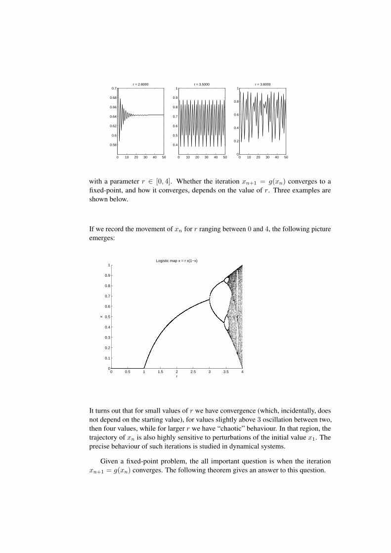
0 10 20 30 40 50

0.58

0.6

0.62

0.64

0.66

0.68

0.7r = 2.8000

0 10 20 30 40 50

0.4

0.5

0.6

0.7

0.8

0.9

1r = 3.5000

0 10 20 30 40 500

0.2

0.4

0.6

0.8

1r = 3.8000

with a parameter r ∈ [0, 4]. Whether the iteration xn+1 = g(xn) converges to afixed-point, and how it converges, depends on the value of r. Three examples areshown below.

If we record the movement of xn for r ranging between 0 and 4, the following pictureemerges:

0 0.5 1 1.5 2 2.5 3 3.5 40

0.1

0.2

0.3

0.4

0.5

0.6

0.7

0.8

0.9

1Logistic map x = r x(1−x)

r

x

It turns out that for small values of r we have convergence (which, incidentally, doesnot depend on the starting value), for values slightly above 3 oscillation between two,then four values, while for larger r we have “chaotic” behaviour. In that region, thetrajectory of xn is also highly sensitive to perturbations of the initial value x1. Theprecise behaviour of such iterations is studied in dynamical systems.

Given a fixed-point problem, the all important question is when the iterationxn+1 = g(xn) converges. The following theorem gives an answer to this question.

Theorem 11.1.4. (fixed-point theorem) Let g be a smooth function on [a, b]. Assume

1. g(x) ∈ [a, b] for x ∈ [a, b], and

2. |g′(x)| < 1 for x ∈ [a, b].

Then there exists a unique fixed-point x = g(x) in [a, b] and the sequence {xn}defined by xn+1 = g(xn) converges to x. Moreover,

|xn+1 − x| ≤ λn|x1 − x|

for some λ < 1.

Proof. Let f(x) = g(x) − x. Then by (1), f(a) = g(a) − a ≥ 0, and f(b) =g(b)− b ≤ 0. By the intermediate value theorem, there exists an x ∈ [a, b] such thatf(x) = 0. Hence, there exists x ∈ [a, b] such that g(x) = x, showing the existence ofa fixed-point.

Next, consider xn+1 = g(xn) for n ≥ 1, and let x = g(x) be a fixed-point. Then

xn+1 − x = g(xn)− g(x).

Assume without lack of generality xn > x. By the mean value theorem there exists aξ ∈ (x, xn) such that

g′(ξ) =g(xn)− g(x)

xn − x,

and hencexn+1 − x = g′(ξ)(xn − x).

Since ξ ∈ [a, b], assumption (2) gives g′(ξ) ≤ λ for some λ < 1. Hence,

|xn+1 − x| ≤ λ|xn − x|≤ · · ·≤ λn|x1 − x|.

This proves the convergence. To show uniqueness, assume x, y are two distinct fixed-points of g with x < y. By the mean value theorem and assumption (2), there existsξ ∈ (x, y) such that

g(x)− g(y)

x− y= g′(ξ) < 1.

But since both x and y are fixed-points, we have

g(x)− g(y)

x− y= 1,

so we have a contradiction and x = y.

Example 11.1.5. Let’s look at the functions from the example (11.1.2) to see forwhich one we have convergence.

1. g1(x) = x − x3 − 4x2 + 10 on [a, b] = [1, 2]. Note that g(1) = 6 6∈ [1, 2],therefore assumption (1) is violated.

2. g2(x) = 12(10− x3)1/2. The derivative is given by

g′2(x) =−3x2

4(10− x3)1/2,

and therefore g′2(2) = −2.12. Condition (2) fails.

3. The third formulation is

g3(x) =

(10

4 + x

)1/2

The derivative is given by

g′3(x) =−5

(4 + x)3/2√

10,

and therefore the function is strictly decreasing on [1, 2]. Since g3(2) =√

5/3and g3(1) =

√2 are both in [1, 2], condition (1) is satisfied. Furthermore,

|g′3(x)| ≤ 1/√

10 < 1 for x ∈ [1, 2], so condition (2) is also satisfied. Itfollows that the iteration xn+1 = g3(xn) converges to a fixed-point of g3. Wecan try this out:

x1 = 1.5, x2 = 1.3484, x3 = 1.3674, x4 = 1.3665, . . .

We can apply the fixed-point theorem to Newton’s method. Let

g(x) = x− f(x)

f ′(x).

Then

g′(x) = 1− f ′(x)

f ′(x)+f(x)f ′′(x)

f ′(x)2=f(x)f ′′(x)

f ′(x)2.

Let α be a root of f . Then f(α) = 0 and f ′(α) 6= 0, so that

g′(α) = 0.

Hence, |g′(α)| < 1 at the fixed-point. Now let ε > 0 be small and a = α − ε,b = α+ ε. Then, by continuity,

|g′(x)| < 1

2

for x ∈ [a, b], and (2) holds. Furthermore,

|g(x)− α| = |g′(ξ)||x− α| ≤ 1

2|x− α| < ε

for x ∈ [a, b]. Hence, g(x) ∈ [a, b] and (1) holds. It follows that in a small enoughneighbourhood of a root of f(x), Newton’s method converges to that root (providedf ′(x) = 0 at that root).

Note that the argument with ε illustrates a key aspect of Newton’s method: itonly converges when the initial guess x1 is close enough to a root of f . What “closeenough” means is often not so clear. Recall that the fixed-point theorem guaranteesconvergence of an iteration xn+1 = g(xn) to a unique fixed-point of g in an interval[a, b] if g(x) ∈ [a, b] for x ∈ [a, b], and |g′(x)| < 1 on [a, b]. We can apply this toshow that Newton’s method converges if we start with an x1 that is sufficiently closeto a root of f(x)4. Newton’s method for finding a root of a continuously differentiablefunction f(x) is a fixed-point iteration with

g(x) = x− f(x)

f ′(x).

The derivative is

g′(x) = 1− f ′(x)

f ′(x)+f(x)f ′′(x)

f ′(x)2=f(x)f ′′(x)

f ′(x)2.

If α is a root of f , that is, f(α) = 0, and if f ′(α) 6= 0, then

g′(α) = 0.

Since g′(x) is continuous, for every δ > 0 there exists an ε > 0 such that |g′(x)| < δfor |x− α| < ε. In particular, |g′(x)| < 1/2 in a small interval [a, b] with a = α− ε,b = α+ ε. By the mean value theorem there exists ξ ∈ (a, b) such that

|g(x)− α| = |g′(ξ)||x− α| ≤ 1

2|x− α| < ε

for x ∈ [a, b]. Hence, g(x) ∈ [a, b] and both conditions of the fixed-point theorem aresatisfied. Newton’s method, interpreted as fixed-point iteration, converges. In the nextsection we derive a stronger result for Newton’s method, namely that it convergesquadratically if the starting point is close enough.

11.2 Rates of convergence

The speed of iterative numerical methods is characterised by the rate of convergence.

Definition 11.2.1. The sequence xn, n ≥ 0, converges to αwith order one, or linearly,if

|xn+1 − α| ≤ k|xn − α|4Sufficiently close means that there exists an interval around the root such that the method converges

for any starting point in that interval.

for some 0 < k < 1. The sequence converges with order r, r ≥ 2, if

|xn+1 − α| ≤ k|xn − α|r

with k > 0. If the sequence converges with order r = 2, it is said to convergequadratically.

Example 11.2.2. Consider the sequence xn = 1/2rn

for r > 1. Then xn → 0 asn→∞. Note that

xn+1 =1

2rn+1 =1

2rnr=

(1

2rn

)r= xrn,

and therefore |xn+1 − 0| ≤ 1 · |xn − 0|r. We have convergence of order r.

For example, if a sequence converges quadratically, then if |xn − α| ≤ 0.1, in thenext step we have |xn+1−α| ≤ k ·0.01. We would like to show that Newton’s methodconverges quadratically to a root of a function f if we start the iteration sufficientlyclose to that root.

Theorem 11.2.3. Let g be continuously differentiable in the neighbourhood of a fixedpoint α. The fixed-point iteration xn+1 = g(xn) converges quadratically to α, ifg′(α) = 0 and the starting point x1 is sufficiently close to α.

Again, sufficiently close means that there exists an interval [a, b] for which thisholds.

Proof. (*) Consider the Taylor expansion around α:

g(x) = g(α) + g′(α)(x− α) +1

2g′′(α)(x− α)2 +R,

where R is a remainder term of order O((x− α)3). Assume g′(α) = 0. Then

g(x)− g(α) =1

2g′′(α)(x− α)2 +R.

Assume that |x− α| < ε. Since R is proportional to (x− α)3, we can also write

g(x)− g(α) =1

2g′′(α)(x− α)2(1 +

2

g′′(α)·R1),

where R1 = R/(x − α)2 = O((x − α)) ≤ Cε for a constant C. Taking absolutevalues, we get

|g(x)− g(α)| ≤ k · |x− α|2.

for a constant k. Set x = xn, xn+1 = g(xn), α = g(α). Then g(x)−g(α) = xn+1−αand

|xn+1 − α| ≤ k|xn − α|2.

This shows quadratic convergence.

Corollary 11.2.4. Newton’s method converges quadratically if we start sufficientlyclose to a root.

In summary, we have the following points worth noting about the bisection methodand Newton’s method.

• The bisection method requires that f is continuous on [a, b], and that f(a)f(b) <0.

• Newton’s method requires that f is continuous and differentiable, and moreoverrequires a good starting point x1.

• The bisection method converges linearly, while Newton’s method convergesquadratically.

• There is no obvious generalisation of the bisection method to higher dimension,while Newton’s method generalises easily.

11.3 Newton’s method in the complex plane

Before discussing Newton’s method in higher dimensions, we present yet anotherexample illustrating the intricate behaviour of fixed-point iterations, this time over thecomplex numbers.

Example 11.3.1. Consider the function

f(z) = z3 − 1.

This function has exactly three roots, the roots of unity

zk = e2πik3

for k = 0, 1, 2. As in the real case, Newton’s method

zn+1 = zn −f(zn)

f ′(zn)

converges to one of these roots of unity if we start close enough. But what happens atthe boundaries? The following picture illustrates the behaviour of Newton’s methodfor this function in the complex plane, where each col or indicates to which root astarting value converges:

If we look at the speed of convergence, we get the following picture: