F0'

DTISEL ECTE

~OF S zB D

NUMERIC MODEL OF ACO 2 LASER AMPLIFIER

THESIS

Frank Patrick GallagherCaptain, USAF

AFIT/GSO/ENP/ENS/89D.2

DEPARTMENT OF THE AIR FORCE

AIR UNIVERSITY

AIR FORCE INSTITUTE OF TECHNOLOGY

Wright-Patterson Air Force Base, Ohio

-p--- ubmq 89 12 26 141

q

AFIT/GSO/ EN P/ENS/89D-2

NUMERIC MODEL OF ACO 2 LASER AMPLIFIER

THESIS

Frank Patrick Gallagher

Captain, USAF

AFIT/GSO/ENP/ENS/89D-2

DTICS ELECTE

DEC271 M I I1B U

Approved for public release; distribution unlimited. . . . .

AFIT/GSO/ENP/ENS/89D-2

NUMERIC MODEL OF A CO 2 LASER AMPLIFIER

TIESIS

Presented to the Faculty of the School of Engineering

of the Air Force Institute of Technology

Air Univ- .sity

In Partial Fulfillment of the

Requirements for the Degree of

Master of Science in Space Operations

Frank Patrick Gallagher, B.S.

Captain, USAF

December, 1989

Approved for public release; distribution unlimited.

Preface

The goal of this thesis was to develop and validate a CO 2 laser amplifier model

that could be used both as a &dsign aid and an instructional tool. As a design aid, the

model's consideration of amplifier physics had to be thorough enough to provide accurate

data while allowing the user to vary many design parameters. As an intructional tool, the

model's user interface had to be simple and straightforward so the student would spend

less time learning how to use another computer program and more time learning laser

amplifier concepts.

In the chapters that follow, I describe the development and validation of this model

as well as the limitations on its performance. In my writing, I assumed that readers of

this tlicsis will have been introduced to CO 2 laser physics. As preliminary reading, I

recommend the papers by Gilbert (7) and Patel (16).

I would like to thank my advisors, Dr. D. 1I. Sto, Dr. T. S. K,-lso, and Dr. D. E.

Beller, for their time and effort in helping me complete this project.

Frank Patrick Gallagher

Aaooeaesson l

DTIC TARB 3UnannounoedJuetifioati-

By/ Distrlbuttoa

Availabi1lty Codes

V jAvail and/orVint Special

II I

Tab.e of Contents

Page

Preface .......... .. ........................................ ii

Table of Contents .......... .................................. iii

List of Figures ........... .................................... vi

List of Tables ........... .................................... viii

Abstract .......... ....................................... ix

I. Background .......... .................................. 1-1

1.1 Original Model ........ .......................... 1-1

1.2 Added Parametero....... . ........................ 1-1

1.3 Amplifier Significance ........ ...................... 1-2

1.4 PurpOse and Scope ........ ........................ 1-3

Ii. Model Development ......... ............................. 2-1

2.1 Amplifier Fundamentals ....... ..................... 2-1

2.2 Amplifier Modeling ....... ........................ 2-2

2.2.1 Basic Amplifier Equation ..... ................ 2-4

2.2.2 Additional Calculations ...... ................. 2-5

2.2.3 Step-by-Step ....... ....................... 2-5

2.2.4 Effects to be Modeled ...... .................. 2-7

2.3 ASE Fundamentals ....... ........................ 2-7

2.3.1 Population of the Upper Vibrational Level ...... .... 2-8

2.3.2 Solid Angle ....... ........................ 2-11

2.3.3 Gain Coefficient ........................... 2-12

iii

Page

2.4 Reflected ASE ......... .......................... 2-14

2.4.1 Equations for Reflected ASE ..... .............. 2-14

2.4.2 Combining the ASE Terms ..... ............... 2-17

2.5 Reflected Input Pulse ........ ...................... 2-18

2.6 Summary .......... ............................. 2-20

I1. V'iidation ............ .................................. 3-1

3.1 Amplification ......... ........................... 3-1

3.1.1 Conditions for Closed Form Solution .... ......... 3-1

3.1.2 Comparison to the Frantz-Nodvik Solution ...... .... 3-2

3.2 ASE ........... ................................ 3-7

3.2.1 Prediction Formulation ...... ................. 3 -

3.3 Reflected ASE .......... .......................... 3-9

3.4 ASE Trend Comparison ....... ..................... 3-11

3.5 Reflected Input Pulse ........ ...................... 3-14

3.6 Summary .......... ............................. 3-15

IV. Results ............ .................................... 4-1

4.1 Determining a Practical Time Step ...... ............... 4-1

4.2 Amplification Using ' 2 C and 13C ...... ................ 4-4

4.3 Temperature Dependence ........ .................... 4-5

4.4 Amplification with ASE Effects ....................... 4-10

4.5 Summary .......... ............................. 4-13

V. Conclusions and Recommendations ........ .................... 5-1

Appendix A. Notes to User .......... .......................... A-1

A.1 General Guidance ......... ........................ A-1

A.1.1 Time Step Effect on Run Time and Memory Limits. A-1

iv

Page

A.1.2 Parameter Limits ....... .................... A-3

A.2 Filed-Pulse Routine ........ ....................... A-4

A.3 Square-Pulse Routine ........ ...................... A-5

A.4 Screen Displays ......... .......................... A-5

A.5 Storing Files ......... ........................... A-6

A.6 Overcoming Memory Limitations ...... ................ A-7

Appendix B. Derivation of Factor1 ......... ...................... B-1

Appendix C. ASE Analytic Solution ....... ..................... C-1

C.1 Basic Equation ........ .......................... C-1

C.2 Analysis of Assumptions ........................... C-1

Appendix D. ASE Variations Due to Large Solid Angles ..... .......... D-1

Bibliography ........ ..................................... BIB-1

Vita ......... .......................................... VITA- I

v

List of Figurcs

Figure Page

2.1. Pulse growth and energy extraction ....... .................... 2-2

2.2. Diagram of Douglas-Hamilton model ....... .................... 2-3

2.3. Typical gain profile after a pulse has been amplified ..... ........... 2-8

2.4. Amplification of a square input pulse ....... ................... 2-9

2.5. Amplification of an oscillator's output pulse (curve A) .............. 2-10

2.6. Relative intensity for ASE traveling in both directions .............. 2-11

2.7. Comparison between the theoretical and the modeled ASE lineshape . 2-12

2.8. Angle defining solid angle limits of integration ..... .............. 2-13

2 Q. ASE parameter trends in the saturation limit: Gain vs Length ..... 2-15

2.10. ASE parameter trends in the saturation limit: Gain vs Diameter . ... 2-15

2.11. ASE parameter trends in the saturation limit: Diameter vs Length . . . 2-16

2.12. Maximum divergence angles for ASE (Q2) and reflected ASE (Q2') . . 2-17

2.13. Range of divergence angles for reflected ASE exiting the amplifier . . . 2-18

2.14. Fraction of ASE+ that can contribute to ASE . .................. 2-19

3.1. Percent error between model and Frantz-Nodvik equation as a function

of time ........... .................................... 3-3

3.2. Percent error between model and Frantz-Nodvik equation as a function

of input pulse intensity ......... ........................... 3-5

3.3. Decrease in percent error as amplifier saturates ................... 3-6

3.4. Amplifier cells modeled for ASE generation ...... ................ 3-8

3.5. Total ASE output as a function of time ...... .................. 3-10

3.6. Gain profile uitder the influence of ASE ...... .................. 3-10

3.7. Total ASE output as a function of time with reflectivity consideration . 3-12

3.8. Gain profile tinder the influence of ASE and reflect(, ASE .......... 3-12

vi

Figure Page

3.9. Rate of gain reduction as reflectivity increases ...... .............. 3-13

3.10. ASE effects on amplifier gain as a function of time and initial gain coefficient 3-14

4.1. Peak pulse output as a function of time step ...... ............... 4-3

4.2. Relative output intensities for 12C and 13C (' 3 C normalized to 1 for both

cases) ............ ..................................... 4-5

4.3. Diagram of the kinetic relationships in a four-level CO2 laser model . . 4-6

4.4. Gain as a function of time and temperature (first cell) ..... .......... 4-8

4.5. Gain as a function of time and temperature (last cell) ..... .......... 4-8

4.6. Output pulse narrowing for increasing temperatures ..... ........... 4-9

4.7. Output power peaks for increasing temperature ...... ............. 4-9

4.8. Gain evolution and ASE output as functions of time ..... ........... 4-11

4.9. Gain as a function of time and pump efficiency under the influence of ASE 4-12

4.10. ASE outputs for various pump efficiencies ..... ................. . -12

4.11. ASE outputs for various window reflectivities ..... ............... 4-13

A.1. Output pulse calculated using (A) 20 cells and (B) 60 cells .......... A-8

vii

List of Tables

Table Page

3.1. Data for Figure 3.2 ........... ............................. 3-5

3.2. Parameter combinations satisfying the three ASE significance criteria in

section 3.4 ............ .................................. 3-15

4.1. Percent change in output intensity ....... ..................... .1-2

4.2. Parameters affected during the temperature dependence test ...... 4-7

A.1. Influence of time step on the number of program integrations. Length =

2 meters, tcav = 10 nanoseconds, tmax = 20 ...... ............... A-2

C.1. Relationship between gain coefficient and the ratio N 2 /(.V 2 - .%I) . . . C-2

C.2. Comparison between solid angle approximation and an integral solution C-3

viii

A FIT/GoJ/ EN P/ ENS/89D-2

Abstract

A CO.,' !r amplifier simulation model is developed for use on IB.M-compatible

personal computers. First, a general laser amplifier is modeled by dividing an amplifier

iwto separate cells to model both the temporal and spatial dependence of the amplifier's

gain. The resulting amplification is validated by comparison with a closed-form solution.

Second, losses due to amplified spontaneous emissions (-ASE) are investigated and iHtcided

;n the model. Equations for ASE losses consider both the solid angle of the emis.sions and

the reflectivity of the cavity windows. Other reflections are ignored. Third, an existing

numerical model of C0 2 gas kinetics is incorporated. In this kinetics model, temperature-

dependent terms are fixed according to initial conditions, and the rotational levels of the

upper C0 2 vibrational state are assumed to be in equilibrium.

The user-friendly model allows designers and students to investigate the amplifica-

tion of either square input pulses or pulses generated with a laser oscilltor while varying

several input parameters. Among the variable parameters are length, diameter, gas mix.

temperature, pressure, window reflectivity, and pump efficiency.

ix

NUMERIC MODEL OF A CO 2 LASER AMPLIFIER

I. Backgroand

As a program, this amplifier model is complete in itself, but it is designed to supple-

ment an existing oscillator model. This chapter will begin with a brief description of the

oscillator model. Next, the need for an amplifier model is presented. Finally, the scope of

this project is outlined.

1.1 Original Model

Recently. a computer simulation model of an atmospheric-pressure, carbon dioxide

(C0 2 ) laser oscillator was developed by Major David Stone. The model is programmed

in Quick BASIC for use on iBM-compat2le personal computers. It has been used in in-

troductory la-ser physics courses to give students an appreciation for the design of laser

radar transmitters. Stone's model uses a numeric approach similar to the one outlined by

Gilbert (7). This model traces the time-varying populations of the 001 and 100 vibrational

levels of CO 2 and the metastable (v=l) level of nitrogen under the influence of an idealized

pump, gas kinetics, and a growing photon flux. The kinetic relationships between these

gases ai,d the development of a population inversion are described with coupled differen-

tial equations and experimentally-determined rate constants. These equations are solved

iteratively usi ng a fourth-order Runge-Kutta integration method.

1.2 Added Parameters

To make the model more precise, several changes to the original model have been

made. First, Stone uses Witteman's equations for the rate constants used in the differential

equations (25). These equations describe the dependence of the rate constants on pressure

and the relative percentages of the species in the gas mix. Second, work by Melanqon has

been included to model the temperature dependence of the rate constants (13). Third,

1-1

Stone has added an optior that will allow the "ideal" pump to be modeled as a half-

sne-wave rather than a square wave. V'ith all these cha..ges, the model currently allows

the following input parameters; pressure; rclative percentages of C0 2 , nitrogen, helium,

hydrogen, and water vapor; opmperature; and pump pulse shape, duration, and efficiency.

Additional parameters relate directly to aspects of laser radar design. Isctopes of CO 2

vary in their ability to transmit through the atmosphere and have different pulse-forming

characteristics. To help analyze any tradeoffs that may exist, Stone has incorporated the

Einstein coefficients of spontaneous emission for carbon-12 ( 2 C) and carbon-13 ( 13C) as

eetermined by Glazenkov (8:535-536). T'ie last parameter is a decision on whet!,er -;r ,not

to use a Q-switch to create - sharper, more intense pulse. The optimization of Q-switching

is part of laser radar design because the tracking of fast distant objects requires short

intense pulses to provide high-resolution range measurements (6:2).

1.3 Amplifier Significance

Stone's model does not treat every aspect oi laser radar design. Two missing con-

siderations deal with power limitaticis. Thy are frequency stability and mirror damage.

A laser radar system determines the velocity of a target by measuring the change in fre-

quency of the return signal (Doppler analysis). Accurate velocity measurement requires

high-frequency stability. Ihis requirement, however, conflicts with the high power required

for long-range tracking. According to Reilly:

Very often the laser radar must have power levels in excess of a few hundIredwatts (CW or repetitive pulse average power). The use of a simple (CO 2 ) lasercan produce satisfactory frequency stability up to power levels of a few tensof watts. Beyond these power levels the stability of the laser resonator oftenbecomes a problem ... the price of frequency stability, unfortunately, is lowpower (18:60).

Power is also limited by the material used for cavity mirrors. Most available materials

have some absorption at the primary CO 2 laser wavelength, 10.61tm. Therefore, CO 2 lasers

are notorious for inducing mirror damage (11:5077). For example, the damage thresholds

for single crystalline molybdenum and single crystalline copper are 60 and 115 J/cm2

1-2

respectively (23:415). Together, the requirements for high power, frequency stability and

increased mirror life necessitate the use of laser amplifiers.

Several studies have confirmed master oscillator/power amplifier (MOPA) systems

using CO2 lasers to be the most effective laser radar transmitters (10, 18, 26, 9). In this

svstem, the master oscillator generates a low-power, spectrally pure beam. This beam then

propagates through a power amplifier where its energy increases, its pulsewidth narrows,

and its frequency characteristics are preserved.

1.4 Purpose and Scope

To add another dimension to Stone's mod , it is the purpose of this thesis to develop

and validate a model of a CO 2 laser radar amplifier. The key to modeling the pulse

amplification process is determining the population inversion encountered by each slice of

an oscillator's input pulse. Like the oscillator model, this model uses a fourth-order Runge-

Kutta integration method to calculate the inversion at any time. However, the inversion

within the amplifier is not spatially constant, so this model also calculates the inversion

for each axial position within the amplifier.

Factors affecting this inversion included in the model are electrical pumping, colli-

sional relaxation, stimulated emission, amplified spontaneous emission (ASE), and emis-

sions reflected between the cavity windows. The portion of the input pulse that is reflected

back into the amplifier will be considered a loss term and will not contribute to the output

pulse. Emissions that are not axially directed, iiicluding wall reflections, are ignored. Be-

cause this model considers the amplification of only a single pulse, factors that determine

pulse repetition frequency will not be addressed.

1-3

SII. lodel Development

This chapter contains theory applicable to modeling the processes of laser amplifi-

cation and ASE. In general, the amplification process can be described by two nonlinear

differential equations. These equations relate to the coupled relationship between the

growing photon density and the deteriorating inversion. Because the modeled inversion

is influenced by gas kinetics, these equations must be solved with numerical integrations

rather than closed-form solutions. The interested reader is directed to the manuscript by

Schulz-DuBois for a more rigorous treatment of these equations (20). During the following

discussion, variables used in the model will be introduced to provide a clear transition from

theory to modeling.

2.1 Amplifier Fundamentals

Consistent with basic laser theory, we are interested in the interaction between pho-

tons and a medium where a population inversion exists. Both the photon density and

the population inversion vary as functions of time and position within the amplifier. In

actual amplifiers, the population inversion and, consequently, the photon density have a

three-dimensional position function. Measurements taken by McQuillan and Carswell have

shown this function to depend on several parameters (12). Among the parameters listed

are: gas composition, pressure, wall temperature, and tube diameter. A high-power am-

plifier model that incorporates all of these parameters on a two-dimensional level has been

developed by Comly (3). Their model was created for the study of laser fusion and was not

concerned with frequency stability, therefore it cannot be directly applied to the analysis

of laser radar transmitters.

In our one-dimensional model we calculate only the longitudinal time variation of

population inversion and photon density. In other words, we have assumed both variables

to be constant for any cross section of the amplifier. By assuming cross-sectional invariance,

we can also assume the diameter of the input beam is equal to the diameter of the amplifier.

This assumption simplifies our population density calculations.

2-1

In the absence of a photon pulse, the population inversion across the entire amplifier

is also uniform. However, once a pulse of photons enters the cavity, the spatial dependence

of the population inversion cannot be ignored. The leading edge of the pulse experiences

the original full inversion, but because it extracts energy as it propagates through the

amplifier, the amount of energy stored in the inversion is reduced. This loss of energy

results in a smaller population inversion.1 Therefore, the remainder of the pulse will be

amplified by a progressively smaller factor. Figure 2.1 illustrates the exponential growth

p ulse energy

stored energy

extracted energy

position/time

Figure 2.1. Pulse growth and energy extraction

of the leading edge and the resulting change in the energy stored for each position in the

amplifier.

2.2 Amplifier Modeling

One approach to calculating the population inversion as a function of time and po-

sition is presented by Douglas-Hamilton et al. (4:76-77). As shown in Figure 2.2, they

divide the amplifier into N cells, each having a length of L/N. By assuming the inversion

across each cell is constant, the spatial dependence is removed and the calculation for the

inversion is done as a function of time only. With increased values for N, the approxima-

'For every photon emitted by this stimulated emission process, the population of molecules in the upperenergy state is reduced by one and the population of molecules in the lower energy state is increased byone-a net change of two.

2-2

Amplifier Cells

input pulse

1 2 3 N-1 N

Figure 2.2. Diagram of Douglas-Hamilton model

tion for constant inversion within a cell becomes more valid. Therefore, we would expect

increased accuracy in the calculation. Surprisingly, this was not the case for their model.

Their predictions for flux intensity were exactly the same over time, whether N = 1 or N

20. They also assert that:

This independence of N holds for a completely saturated and a completelyunsaturated amplifier, as well as for the case where the amplifier saturatessomewhere along its length. (4:78)

The explanation given is that local gain is only a function of photon density. That is,

their rate constants are reduced to zero. More information on amplifier output without

gas kinetics appears in the validation chapter.

The discussion of their model does not explicitly define the manner in which the

input pulse is divided to "fit" into each cell at each time interval. In Stone's model, the

data for the output pulse is already divided into time units based on his code's time step

(hi) and the average lifetime of a photon within a particular resonator (tcav). For this

reason, we cannot arbitrarily choose any value for N amplifier cells. In this model we will

use the relationship x = ct to define not only the position in the amplifier, but also the

length of each cell. In this equation, c is the speed of light in the medium and t is a unit

of time defined by the number of tcav time units that have elapsed. For example, if tcav

2-3

is 10 nanoseconds and hi is 0.1, the length of one amplifier cell will be 0.3 meters. If the

length of the amplifier is three meters, then it will be divided into 10 cells.

2.2.1 Basic Amplifier Equation. If we allow j to be the time unit under consid-

eration and k to represent a particular cell within the amplifier, the equation for photon

density growth from one cell to the next cell is:

P(j+lk+l) = P(jk) e (k)) L (2.1)

where Pis the number of photons per cubic meter, g is the gain coefficient, a is the loss per

unit distance due to scattering and possible absorption by non-active constituents in the

laser medium, and L is the length of the amplifier cell. The gain coefficient is the product

of the population inversion and a, the stimulated emission cross section. The expression

e(_q-9)L is also known as the small-signal gain and will be represented by the symbol, G.

The population inversion (Nversion(j,k) in the model) is calculated using a slightly

modified version of Stone's numerical method. Basically, the normalization terms have been

removed and the photon density growth now occurs outside the Runge-Kutta integrator.

It must be emphasized here that the validity of this integration method has already been

established, and the validation portion of this modeling effort will only deal with the

actual amplification process (7). As in Stone's code, the stimulated emission cross section

is calculated in this manner:F.(j=9)(A21 )c 2

(2.2)47r2(v)2 .AVP

where A 2 1 is the Einstein coefficient of spontaneous emission, 2 v is the frequency of the

J19 - J20 [P(20)] transition, Avp is the linewidth of the emission, and Fu(jl9 ) is the frac-

tion of molecules in the 001 vibrational level that are in the J = 19 rotational level (7:2535).

In the model, F,(j=l) is calculated as part of the Boltzmann distribution for the rota-

tional levels. The distribution is based on the parameter for initial temperature. We will

assume the rotational thermalization rate to be high enough to maintain this Boltzmann

distribution throughout the amplification process. Rooth has shown the thermalization

2A21 will be described in more detail in the ASE section.

2-4

time to be less than one nanosecond (19:108). So, as long as the input pulse does not

saturate the gain in a nanosecond, we will not need to consider rotational nonequilibrium.

The linewidth of the emission, AvP, is calculated as a function of gas mix, tempera-

ture, and pressure using an equation adapted from Witteman (25:61):

300Avp = 7 .58 ((4 CO, + 0 .7341)N, + 0 .6 4 DHe + 0 .3 2 (DH, + 0.384(H2 o)Pres Temp (2.3)VTemp

where -D represents the percentage of a gas in the mix. For typical gas mixes, the calculation

is valid at pressures (Pres > 0.015 atm) where collision broadening dominates and the

lineshape is approximately Lorentzian (22).

2.2.2 Additional Calculations. Before we look at the iterative steps of the ampli-

fication process, two more calculations will be described. First, the input data must be

converted from megawatts/liter into photons per cubic meter. The derivation of this con-

version constant (Factorl) appears in Appendix B. Second, each input unit is modified

by the transmissivity of the window as it passes through the entrance and exit of the

amplifier. Typically, practical devices have windows with anti-reflective coatings. Anti-

reflective coatings can be designed to allow more than 98 percent of incident light, within

a particular range of frequencies, to pass through the window (17).

2.2.3 Step-by-Step. The amplification process, as modeled here, is a two-step pro-

cess nested in two loops. The outer loop is for the current time step. The inner loop is

for the current cell under consideration. Within this loop both amplification steps occur.

First, a small-signal gain is calculated for that cell using its current population inversion. If

the photon density in that cell was greater than zero at the previous time interval, then the

new inversion will reflect changes due to pumping, collisional relaxation, and spontaneous

emission. Next, using Equation 2.1, the photon density is calculated for the next cell at the

next time unit. These steps are done for each cell before the next cell is considered. Only

after the calculations are completed for all cells (k) is the next time (j) unit considered.

Initially (time unit j = 0), all values for photon density (P(ok)) are set to zero and

an input power value for each time step is stored in a file called Filelnput. Now let's look

2-5

at what happens in the first amplifier cell:

* At j = 0.

1. The small-signal gain is calculated using the population inversion determined

by the Runge-Kutta subroutine.

2. Using Equation 2.1, the photon densitv is calculated for the next cell. In this

case, the value will be zero because the value for photon density in cell 1 was

initialized to zero.

3. Next, the first value from FileInput is multiplied by both Factorl and the win-

dow transmissivity. At this point, it is the photon density value in cell 1 for

j = 1.

9 These steps are repeated for all amplifier cells.

9 At j = 1.

1. The small-signal gain is recalculated for cell 1.

2. Using Equation 2.1, the first value from FileInput is "amplified" to become the

value for photon density in cell 2 at j = 2.

3. Now the next value from FileInput is read in and modified to become the photon

density value in cell 1 at j = 2.

From here let's move on to a point in time where the first value from FileInput is

just about to enter the last cell:

e At j = end - 1.

1. Following all of the other cells, the small-signal gain is calculated for the last

cell.

2. Using Equation 2.1, an output value is calculated. In this case, the value is zero.

3. Finally, the first value from FileInput arrives.

* At j = end.

2-6

1. Again, the small-signal gain is calculated for the last cell.

2. The first value from FileInput is "amplified" one more time and becomes the

output value for j = end + 1. As noted earlier, the length used for amplification

by the last cell may be shorter than the rest of the cells. This fact is included

in the calculation. However, the units used for time are not as flexible. So, the

data table may list a slightly longer time-to-exit than actually occurs.

3. To finish the calculation for this output slice, it must be multiplied by the win-

dow transmissivity and converted from photons per cubic meter to megawatts.

2.2.4 Effects to be Modeled. Two important effects illustrated by this model are

gain saturation and pulse sharpening. Saturation of amplifier gain sets a fundamental limit

on the abilities of the laser system. As noted earlier, the process of anpiification reduies the

population inversion. When the populations of the two coupled levels have been equalized,

the gain is saturated. Figure 2.3 shows the distribution of gain after a pulse has propagated

through the amplifier. In this case, only the last cell has been completely saturated. A

natural consequence of saturation is pulse sharpening. For example, Figure 2.4 compares a

square pulse before and after amplification. Prior to amplification, the energy was equally

distributed throughout the pulse's duration. Afte- amplification, the pulse has most of its

energy located near the leading edge. Figure 2.5 illustrates pulse sharpening during the

amplification of oscillator pulses. Curve A represents the amplifier input. Curves B and C

are the outputs of amplifiers with lengths x and 2z, respectively.

2.3 ASE Fundamentals

In the amplification process presented above, the primary cause of energy loss from

the population inversion is stimulated emission. So far, the only source term for these

emissions is the input pulse. Other source terms that will be modeled are spontaneously

emitted photons. These photons are emitted in all directions, but only those propagating

axially-either forward or backward-will contribute to a significant decrease in the pop-

ulation inversion. The bidirectional increase in ASE intensity is shown in Figure 2.6. In

high-gain amplifiers, ASE output can be both intense and relatively narrow in bandwidth.

2-7

O1

0.8

0.6

0.4

0.2

0 I I I I I I I0 0.1 0.2 0.3 0.4 0.5 0.6 0.7 0.8 0.9 1

POSITION 1N AM::LFIER (PCT OF LENGTH)

Figure 2.3. Typical gain profile after a pulse has been amplified

However, because this output will not have the spectral qualities of an oscillator input

beam, it is useless in a laser radar system. Because this energy extraction is counterpro-

ductive, amplifiers must be designed to avoid unnecessary losses to ASE. Essentially, three

parameters determine whether or not ASE will significantly limit the output of the laser

amplifier:

1. Population of the upper vibrational level.

2. Solid angle for amplification.

3. Gain coefficient.

2.3.1 Population of the Upper Vibrational Level. Molecules in an excited energy

state (E1 ) generate photons by spontaneously dropping to a lower energy state (Eo). The

laser transition for CO 2 molecules is from v = 001 to v = 100. This transition can occur

between any one of over fifty rotational level pairs associated with the excited v = 001

level. Each of these rotational levels emits photons at a unique frequency. In addition, each

2-8

60

40

100

10

0111111111111111.,,,i I1I1M11I1I 1b10o il PLLSa I I I I ,I I o I II II IFIIIIII1

Figure 2.4. Amplification of a square input pulse

level emits photons at a different rate. The rate at which these emissions occur is described

by the Einstein coefficient of spontaneous emission, A21. For example, the transition from

v = 001 to v = 100 on the J = 19 rotational line has a value of 0.194 sec - 1 (8:536). In

our model, we use the product of this constant, the population density of its rotational

level, and the time step to generate the ASE photon density, at a particular frequency,

during one time step. Since A 21 is a constant, and F(j=lg) is assumed to be constant, 3

the parameter that determines how many photons will be spontaneously emitted is the

population density of the upper vibrational level, v = 001. In the model the equation is:

ASEdt = yO(l,k)(F.(j= 9 ))(A21)(tcav x hi) (2.4)

3The model does not recalculate temperature after each iteration, so F.(j.9) is assumed to be constant.Because the validity of this assumption depends on the rate at which temperature increases in the cavity,this model is valid only for pulses with relatively short durations.

2-9

0.9

0.8

z 0.7

0.6

0.5

0.3

0.2 A0.1

0 5 10 15 20 25 30 35 40

ARBITRARY TMl UNTS

Figure 2.5. Amplification of an oscillator's output pulse (curve A)

where "ASEdt" represents the density of photons spontaneously emitted during one time

step and Y0(1.k) is the population density of the upper vibrational state. By multiplying

by F,(j=l9 ), we are calculating the population density of only those photons emitted as a

result of J19 - J20 transitions.

In a conservative approximation, we will calculate the ASE density at line center.

Then, to account for all of the other emissions, we divide that photon density by Fu(J=19).

In this way, we treat each emission line as if all the photons on it are amplified at line center

gain. Our approximation is conservative because the gain at line center is slightly greater

than the gain at the other transition frequencies (16:31). Therefore, we overestimate the

effect of ASE on the population inversion.

To reemphasize this effect, consider that with higher gain at line center more photons

will be generated at that frequency. Since amplification is an exponential process, photons

at line center "win the competition" for the gain and dominate the ASE output. Thus,

ASE has a narrow bandwidth. In fact, the higher the gain in the system, the narrower its

2-10

L

Figure 2.6. Relative intensity for ASE traveling in both directions

line shape gets (24:181-182). Figure 2.7 compares our approximation of the ASE lineshape

to its theoretical 1ine shape.

To compare ASE to the previous amplifier analysis, one can think of each cell as

an input window. At each time interval, each cell contributes more photons to the ASE

'pulse". Some of the ASE photons will travel the same direction as the oscillator input

pulse. Assuming isotropic emission, an equal portion will travel the opposite direction.

-'ASE + " will be used to refer to the copropagating photons and "ASE-" will be used to

refer to the counterpropagating photons.

2.3.2 Solid Angle. Of the photons traveling axially, only a fraction of them will

make it out of the amplifier. In our model, we assume these photons are the only ones that

significantly affect the gain in the amplifier. If we neglect wall reflections, this fraction can

be approximated in terms of solid angles. The photons are emitted into a solid angle of

4,r steradians. The fraction traveling in the proper direction is Q/47r, where Q is the solid

angle subtended from a point in the amplifier to the appropriate wall. There are two solid

angles for each position in the amplifier, one for ASE+ and one for ASE-. For amplifiers

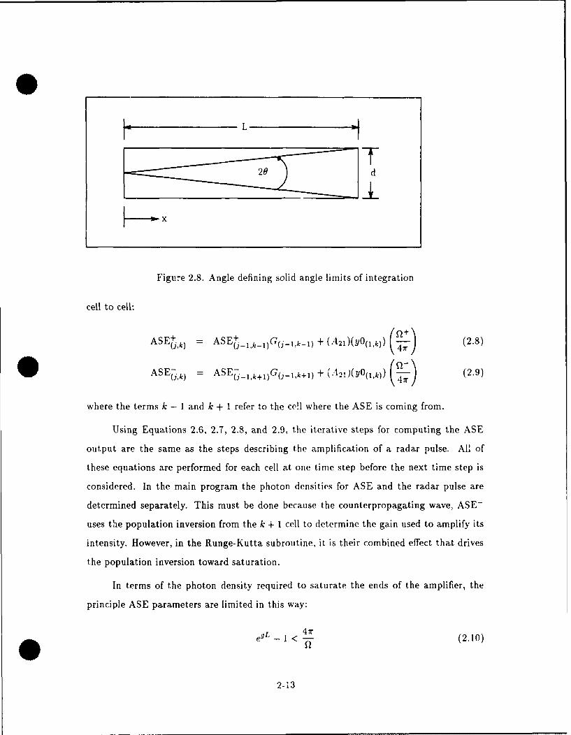
with circular cross sections. f1 is given by:

Q= 27rsinOdO (2.5)

where 0 is the angle illustrated in Figure 2.8 (21:528-529). The solution to the integral has

2-11

1 APPR0)G.4ATMtI xtA-I0.8

CAcTALCtd L #

OL2

2. 89E+ 13 2..F+'3 +1'3 2.8311E+13 2.a311E+l 32 3OM + 13 2 .2 1 3C 2- E+13 Z8313E 13

FREQUJENCY (i-tz)

Figure 2.7. Comparison between the theoretical and the modeled ASE lineshape

the forms:

Q = 2,r I- (2.6)

Q- 27r -1 /) (2.7)

for ASE + and ASE-, respectively. In these equations, L is the length of the amplifier, xr is

the axial position, and d is the diameter of the circular aperture (:2033-2034). Clearly, the

fraction of photons that contribute to ASE is a function of amplifier length and diameter.

2.3.3 Gain Coefficient. Thus far, we have an equation for calculating the amount of

ASE each cell adds at each time interval and an equation for the fraction of those photons

having a direction that allows them to contribute to the ASE output. With the addition

of the small-signal gain term, we arrive at the equations used for propagating ASE from

2-12

I_ L 1

T20 d

I- -I

-X

Figure 2.8. Angle defining solid angle limits of integration

cell to cell:

ASEj~k - ASE+j_I,kI)G('_I,k_1) +(A21)(yO(l.k))(28ASE- A SE-_ G_1,k ) + (2.8)

ASEk) = ASE ik+)G(j_,k+)+ (A2)(YO(lk)) (2.9)

where the terms k - 1 and k + 1 refer to the ce!l where the ASE is coming from.

Using Equations 2.6, 2.7, 2.8, and 2.9, the iterative steps for computing the ASE

output are the same as the steps describing the amplification of a radar pulse. All of

these equations are performed for each cell at one time step before the next time step is

considered. In the main program the photon densities for ASE and the radar pulse are

determined separately. This must be done because the counterpropagating wave, ASE-

uses the population inversion from the k + I cell to determine the gain used to amplify its

intensity. However, in the Runge-Kutta subroutine, it is their combined effect that drives

the population inversion toward saturation.

In terms of the photon density required to saturate the ends of the amplifier, the

principle ASE parameters are limited in this way:

egL 1 < 47r (2.10)

2 -13

where Q is a function of length and diameter. The details of Equation 2.10 will be discussed

in Appendix C. The simplest approximation for Q is .4L, where A is the cross-sectional

area of the amplifier and L is its length (14:399). For circular cross sections, the equation

for preventing saturation is now:

16L 2 (2.11)e9- 1< d (.11

Figures 2.9, 2.10, and 2.11 illustrate these limitations graphically. Figure 2.9 shows how

sensitive diameter is to changes in initial gain and length. Similarly, Figure 2.10 shows

how sensitive length is to changes in initial gain and diameter. Figure 2.11 shows how

length and diameter can limit the initial gain.

2.4 Reflected ASE

The effect of ASE on amplifier gain is even more significant if we consider the reflec-

tivity of the cavity windows. Now the amplifier acts like an oscillator, and the intensity of

ASE grows until the gain drops off significantly. Thus, window reflectivity is an important

design parameter. In fact, analysis has shown that decreasing window reflectivity is the

most effective way to circumvent ASE limitations on amplifier gain (2:147). The following

numeric example will demonstrate the importance of window reflectivity. We start with

1 x 109 ASE photons at one end of a 15-meter amplifier with a constant gain profile. The

gain coefficient at line center is 100 percent per meter. Fifty nanoseconds later the ASE

photons have traversed the cavity and have grown to 3.3 x 1015. If only a tenth of one

percent is reflected, there will be 3.3 x 1012 photons headed back toward the other er.d of

the ca.ity-over 3000 times the number we had initially.

2.4.1 Equations for Reflected ASE. Not all ASE that is reflected will propagate the

entire length of the amplifier. We should recall that the photons had to be emitted into a

small solid angle to make it to the reflecting surface. Additionally, this solid angle varied

depending on the emission's position within the amplifier. If we think of the solid angle as

an angle of divergence, it is obvious that a. even smaller angle £2' is required for ASE to

be able to reflect off one end and exit the opposite end. Figure 2.12 shows these two angles

2-14

10A1

3 as

02

0X4 08 08 1 1.2 1.4AIRMARY LDJGTH

Figure 2.9. ASE parameter trends in the saturation limit: Gain vs Length

IL

0.8

0.6

0Q4

0.2

0 0.04 0.C8 0.12 0.16 0.2AReITRARY DIAMTER

Figure 2.10. ASE parameter trends, in the saturation limit: Gain vs Diameter

2-15

GAIN

0.8

0.2

0I i i

0.40 0.60 0.80 1.00 1.20 1.40

ARBTRARY LENGTH

Figure 2.11. ASE parameter trends in the saturation limit: Diameter vs Length

of divergence by unfolding the reflected half of the ASE path. Both angles increase for

emission positions closer to the end of the amplifier. In the model, each cell's contribution

to the ASE output includes a calculation for the fraction of photons that are emitted into

2'. The equations for this "reflectable fraction"are:

Q1,+ = 7r(d/2)2 1 (2.12)(2L - X) 2

(+

Q_ ir(d/2) 2 1 (2.13)

(L + x) 2 (-

for reflected ASE + (ASE + ) and reflected ASE- (ASE-), respectively (1:2039). The equa-

tions for their amplification are:

ASE+ = l'+ASEdt + ASE - G (2.14)

rLj,k = (-1k

ASE = fl'ASEdt ASESE G (2.15)

r(.jk) S+S-12-k+1)

2-16

LI- 2L -

Figure 2.12. Maximum divergence angles for ASE (Q) and reflected ASE (Q')

These values will be amplified alongside ASE + and ASE-. However, they will not affect

the population inversion. They are monitored strictly to determine the amount of ASE

that will reenter the medium and contribute to the power output at the opposite end.

For example, let us consider the end of the medium where x = L. Without a

reflected contribution, ASE- has a population density of A21yO(1,k)f-/4r (ASEdt in the

code). Reflection adds to ASE- the present value for ASE + multiplied by the window

reflectivity. The only remaining calculation to be done is to determine what fraction of

ASE + can now become a source for ASE-.

2.4.2 Combining the ASE Terms. Figure 2.13 shows that the ASE + photons that

arrive at the end of the cavity have a divergence angle between (small-angle approxima-

tions) d/L and d/2L. The larger angle includes those photons generated close to the

reflecting surface and the smaller angle includes those generated neai the end of the ampli-

fier. To continue our conservative approach, we will assume all of the photons arrive with

the smaller divergence angle. With this assumption. Figure 2.14 shows that 9 of the ASE+

photons can be added to ASE-. These photons, reduced by the reflectivity of the first

window will be reflected one more time before exiting the amplifier. In effect, we monitor

two reflections for any cell's ASE photons. We assume further reflections have a negligible

effect on the overall ASE intensity. Thus, the equations for ASE- and ASE7 in the last

2-17

2L1

LT

Figure 2.13. Range of divergence angles for reflected ASE exiting the amplifier

amplifier cell are as follows:

ASE-'k) = ASEdt + R (ASE+jl,k)) (2.16)

ASE-jk) - (ASEdt) + R? (ASE~j I, k) ) (4) (2.17)

with R representing the reflectivity of the cavity window. Parallel equations are used to

calculate ASE + and ASE + in the first cell.

Putting all the ASE equations together, certain phenomena are expected in simple

cases where gain is independent of gas kinetics. If the reflectivity is zero, the ASE output

intensity will increase until all points inside the amplifier are contributing to the output.

The time period for this increase is the time required for a photon to travel the length

of the amplifier. After this time, the intensity remains relatively constant, decreasing as

the population inversion is depleted. If the reflectivity is greater than zero, the population

inversion is depleted much more rapidly. With a reflected contribution to ASE at the ends

of the amplifier, the ASE intensity continues to grow until the gain is saturated.

2.5 Reflected Input Pulse

The last loss term included in this model is also a result of window reflectivity.

Like ASE, the input pulse itself can be reflected back into the amplifier and reduce the

2-18

S

AArea2

Area2AAeal A4/9

Figure 2.14. Fraction of ASE+ that can contribute to ASE-

population inversion. However, this reflection tends to dampen itself out rather than

grow exponentially. For example, let's say that an input intensity of 100 W/cm2 exits

the amplifier with an intensity of 500 W/cm 2. We'll assume there are no anti-reflective

coatings, so we can expect up to four percent reflection. Therefore, 20 W/cm2 will reenter

the cavity. Though this is only 1 the amount we started with, it cannot be neglected. It

will still affect the gain that the remainder of the pulse experiences.

Modeling this phenomena is much simpler than modeling reflected ASE. Because all

of the photons in the pulse are traveling the same direction there are no solid angles to

calculate. Assuming the photons leave the amplifier only through one of the windows, the

following five equations describe their cyclic flow. We start with the initial reflection:

r(j,k= ast) = ( P(j-lk=last)) . (2.18)

Now we have a reflected pulse traveling in the negative direction. It is amplified according

to:

jk) (k+1))()(

2-19

until it reaches the beginning of the amplifier where it is reflected once more:

rP+'kR1) - -1.k=1)) -(2.20)

Again, it is amplified as it propagates in the positive direction:

Finally, the pulse arrives at the end of the amplifier where it is reflected together with any

of the input pulse that may still be passing through the amplifier:

Pjkls) (P o-1.&=ast)) + R? (P(jl,k=1ast)) (2.22)

The last four equations are then used for the remaining cycles to calculate the gain reducing

terms, P+ and P,-.

2.6 Summary

In addition to gas kinetics and electrical pumping, this model simultaneously moni-

tors four other gain-reducing terms. In order of appearance, they are: ASE, reflected ASE,

the input pulse, and its reflection. These terms are added in the Runge-Kutta subroutine

to form a single value for the photon denst. This value is used Lo calculate new popula-

tions for the v = 001 and v = 100 states of CO 2 in each cell for each time interval. After

the populations are returned from the subroutine, the gain in each cell is determined. The

gain is then used to calculate the growth of each of our monitored terms. The next chapter

describes the validation of each of these modeled processes.

2-20

IH. Validation

3.1 Amplification

The validation process for a computer model begins with a series calculations to

verify each equation and algorithm. Once the step-by-step correctness is established, the

model is ready for direct comparison to experimental results or a theoretical comparison

to results calculated with an analytical solution. One advantage of an analytical solution

over published experimental results is the ability to freely adjust the input parameters.

By varying the inputs over a wide range, it is possible to determine trends in the errors

produced by the model. These trends establish the boundaries within which the model pro-

duces reasonable output. To validate our amplifier model, we used the analytic equations

derived by Frantz and Nodvik for the amplification of a "square" pulse1 (5:2348).

3.1.1 Conditions for Closed Form Solution. To arrive at their solution, Frantz and

Nodvik used four simplifications. First, they assume a two-level system, meaning the sum

of the number densities for the upper and lower states is constant. Second, they neglect

any frequency dependence by assuming the input beam to be monochromatic. Third, they

neglect spontaneous emissions. With this assumption, only the input pulse plays a role in

changing the population inversion. Fourth, they assume the population inversion varies

only one dimensionally and that it is initially uniform across the amplifier.

To duplicate these conditions, our model was both enhanced and constrained. The

enhancement was a new set of input parameters to create "square" pulses and allow any

initial gain setting. We already assume line center operation, so no adjustment was nec-

essary for their monochromatic assumption. The remaining assumptions were duplicated

by constraining our rate equations. In the equation for ASE, A 2 1 was set to zero, thus

eliminating any spontaneous emissions. In the equations for collisional relaxation, the de-

generacy ratio was set to one and all of the rate constants and pump terms were set to zero.

In effect, we turned off the kinetics and allowed the population inversion to be reduced

only by the stimulated emission process.

'"Square" refers to constant amplitude with rise and set times of zero.

3-1

The result of all these adjustments was a clean validation environment where the dif-

ferences between our results and those obtained with the Frantz-Nodvik equations were not

related to pumping, collisional relaxation, or ASE. Also, we were able to compare both long

and short pulses. If we had left the kinetics on, we would have been limited to pulse dura-

tions on the order of tens of nanoseconds because the Frantz-Nodvik solution is "justified

(only) during times small compared to the radiative lifetime of the excited state"(5:2346).

Furthermore, such a time scale would have required consideration of nonequilibrium among

the rotational levels of the excited state. This consideration is beyond the scope of our

model. So, to validate our model on a theoretical level, we used a clean, "kinetic-less"

environment.

3.1.2 Comparison to the Frantz-Nodvik Solution. The Frantz-Nodvik equation for

a square pulse traversing an amplifier with initially uniform gain expresses photon density

as a function of time and position in the amplifier:

tno= 1- [1- exp(-oAox)] exp[-2oar(t - (3.1)

where n is the photon density, AO is the initial population inversion, 17 is the total number

of photons per unit area of the pulse, and 7 is the pulse duration (5:2348). This equation

was used to compare amplifier output on a point-by-point basis.

First, we simply compared outputs for t = LIc, where L is the amplifier length. This

is the instant in time when the leading edge exits the amplifier. As mentioned before, the

leading edge is the only part of the pulse to see the full inversion. As expected, both the

equation and model had the leading edge amplified exactly by egL. Figure 3.1 compares

the outputs for t > L/c. The curves were generated using a high-gain (160 percent Pcr

meter), one-meter amplifier and a large input pulse (6 MW/cm 2 ). Here we note the error

between values based on integration over a few cells (the model) and an infinite number of

cells (the Frantz-Nodvik equation). Both curves start at zero error. 2 The lower curve in

2The initial error is zero because the leading edge of the pulse experiences a constant gain profile.Therefore, its amplification is described by e9 g .

3-2

7

2

01 T _ ! I [

0 10 20 30 40 50 60 70 80 90 100PULSE DURATION (Inzr .... ,5)

Figure 3.1. Percent error between model and Frantz-Nodvik equation as a function oftime

Figure 3.1 shows the overall error reduction if the amplifier is divided into tvice as many

cells.

The error is due to the fact that the model only approximates the positional depen-

dence of gain. We still have constant gain across each cell. Smaller and smaller cells are

required to describe the gain profile if the gain is changing radically from point to point.

Separately or together, three factors increase our model's error. Basically, they all have to

do with the intensity of the pulse inside the amplifier. Obviously, if we start with a large

input pulse, the gain will change rapidly. But, even if we start with a small -ulsf., large

gain can cause the pulse to grow large enough to saturate the end of the amplifier. If we

start with a small pulse and small gain, but the amplifier is very long, the same effects

occur. The only way to limit errors under these conditions is to divide the amplifier into

as many cells as patience and computer memory will allow.

The convergence toward zero error by both curves in Figure 3.1 is a direct result of

3-3

reduced gain. As the amplifier becomes saturated, the pulse sustains a smaller growth rate.

For this limit, where every excited atom in the amplifier decays, Frantz and Nodvik have

derived an equation for the energy gain. Energy gain is the ratio of the energy contained

in the output and the input pulses:

GE = nL(t)dt no(t)dt . (3.2)

For a square pulse the Frantz-Nodvik equation foi energy gain is

GE = (2I)ln{1 + exp( ooL)[exp(2o,77)- 1]} (3.3)

where 77 is the total number of photons per unit area in the pulse (5:2348). We used this

equation to determine the trends in error associated with the model's premature saturation

of the amplifier. Error was calculated by the equation

G E, - GE:.,,¢) 34%error = 100( modd G QnItc) (3.4)

C Eanoiyt~c

Using a one-nanosecond time step, data was collected for points in time where the error

was at its maximum for various amplifier lengths, initial gains, and input intensities. For

comparison between energy gain error and error as a function of time, the same parameters

that were used to generate Figure 3.1 were used again for this trend analysis. Combining

all the data we collected, Figure 3.2 illustrates a linear relationship between error and

input intensity. Table 3.1 shows that the length of the amplifier is inversely proportional

to the initial gain. That is, if we want to have the same error for an amplifier twice as

long, we must use half of the initial gain. The different slopes of the lines in Figure 3.2

show that among the three variables, error is most sensitive to the initial gain. This is

due to the increased rate of energy extraction associated with higher gain amplifiers. To

accurately model amplifiers with higher gains, we must divide the amplifier into smaller

cells by using smaller time steps. In general, the output pulses from the model will have

the same peak as the analytic solution, but they will be slightly broader.

Though the model extracts the energy from the amplifier at a slightly different rate

3-4

13

12 C11

M 96

4321 Z0,A

0 1 2 3 4 5 6 7NTENSITY (MW/arn2)

Figure 3.2. Percent error between model and Frantz-Nodvik equation as a function ofinput pulse intensity

Table 3.1. Data for Figure 3.2

GAIN COEFFICIENT (% per meter)LENGTH

LINE 1 meter 2 meters 4 meters

A 40 20 10B 80 40 20

C 160 80 40

3-5

than the analytic SOlUtiOn, it approaches the same value for GE in the limit where the

amplifier is completely saturated. Frantz and Nodvik have shown this limiting value to be

GE -, 1 + AoL/2r.

when 2at/> 1 (5:2348). Figure 3.3 shows that as the value for 20t increases linearly, the

error decreases asymptotically to zero.

0.3

0.2:5 -

0.2

~0.15

0.1~0.05

0 1 2 3 4 5 6 7 8 9 10

2*RS--MA*ETA

Figure 3.3. Decrease in percent error as amplifier saturates

A similar result was found in the limit for very small pulses. Pulses of "infinitesimal"

width are amplified according to the exponential law. That is, they experience constant

gain rather than a gain that is reduced in an intensity-dependent fashion. According to

Frantz and Nodvik, a pulse is of infinitesimal width if 2or7 < exp(-AoaL) and its energy

gain is described by:

lim GE = exp(AocL) (3.6)77-0

for finite L (5:2348). By using shorter pulses and/or smaller input intensities, the model's

results approached this limit.

3-6

All in all, these examples indicate that our model's results agree with Frantz and

Nodvik's analytical solution. The energy gain errors are small for both very large and

very small input pulses. More importantly, the time variations of the output power-the

shape of the output pulse-are consistent with those calculated with the Frantz-Nodvik

equations. We have found that this consistency depends on the rate at which the gain

is changing. The users of this model can use Figure 3.2 as a guideline to estimate the

model's errors. They should also keep in mind that using a smaller time step (more

amplifier divisions) can also improve the model's accuracy.

3.2 ASE

Now that we have established the validity of our amplifier model, we can use it as

the basis for validating our ASE calculations. For ASE, each cell is an input window.

During each time step, each cell emits a group of photons into the cavity. As these groups

propagate from cell to cell, they undergo an amplification process identical to that of a

standard input pulse. So, to computationally validate our method for ASE output, we

formed a prediction for the output at one end. Next, we formed a similar prediction to

validate the model's calculation for ASE + ASE, output. Finally, we collected data for

various lengths, diameters, and initial gains to establish trends in the way ASE affects the

population inversion. To validate our model on a broader scale, we compared our trends

to those calculated with Equation 2.11.

3.2.1 Prediction Formulation. To form a prediction for the ASE output at one

end we took advantage of the fact that each cell's contribution is the equivalent of an

infinitesimal pulse. For example, a 30-centimeter cell in the middle of a one-meter amplifier

would generate a photon density of 1.8 x 1010 during one time step if the initial gain

coefficient was 50 percent per meter. 2orr7 for this case is 5.5 x 10 - 13, which is clearly

less than the value for exp(-AOaL), 0.6. Thus, the criteria for an infinitesimal pulse is

satisfied.

Because infinitesimal pulses are amplified according to the exponential law, our pre-

diction is simple to formulate. First, we considered the forward traveling ASE in an

3-7

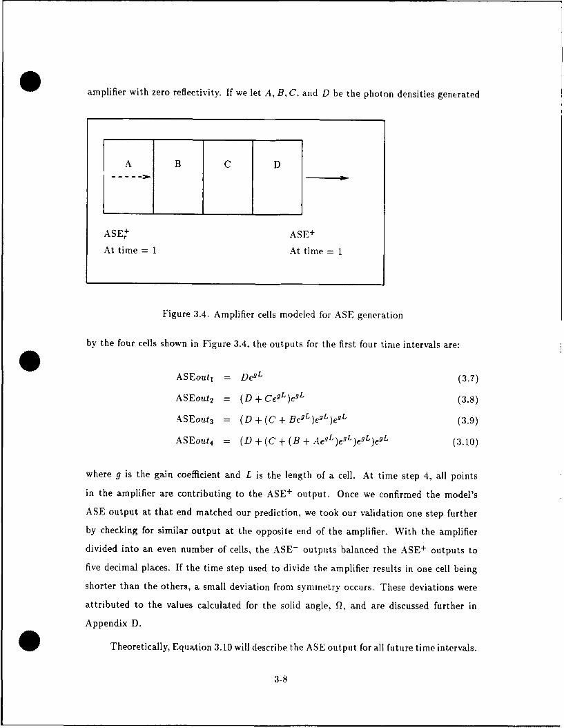
amplifier with zero reflectivity. If we let A, B, C, and D be the photon densities generated

A B C D

ASE + ASE +

At time = 1 At time = 1

Figure 3.4. Amplifier cells modeled for ASE generation

by the four cells shown in Figure 3.4, the outputs for the first four tinie intervals are:

ASEout = De9L (3.7)

ASEout2 = (D + Ce9L)egL (3.8)

ASEout 3 = (D + (C + BeL)e L)eL (3.9)

ASEout4 = (D + (C + (B + AegL)e9L)e9L)e gL (3.10)

where g is the gain coefficient and L is the length of a cell. At time step 4, all points

in the amplifier are contributing to the ASE+ output. Once we confirmed the model's

ASE output at that end matched our prediction, we took our validation one step further

by checking for similar output at the opposite end of the amplifier. With the amplifier

divided into an even number of cells, the ASE- outputs balanced the ASE+ outputs to

five decimal places. If the time step used to divide the amplifier results in one cell being

shorter than the others, a small deviation from symmetry occurs. These deviations were

attributed to the values calculated for the solid angle, Q, and are discussed further in

Appendix D.

Theoretically, Equation 3.10 will describe the ASE output for all future time intervals.

3-8

Eventually though, the population of the excited state molec-iles will show noticeable

decrease. This happens first in cell D. At this point, the values for g and A, B, C, D will

decrease slightly and continue to decrease until the cell is saturated. All of these variables

now have a spatial dependence based on the population of the excited state molecules.

Figures 3.5 and 3.6 illustrate these concepts. Figure 3.5 shows the total ASE output over

time. Starting at zero, it rises to a peak and then decreases as the gain falls off. Figure 3.6

shows the gain profile under the influence of ASE.

Of special note here are the conditions that were set up to show these dramatic ASE

effects. The amplifier was relatively long (9 meters) and broad (10 centimeters). It also

had a gain coefficient of over 200 percent per meter. These conditions are required for

two reasons. Most importantly, the Einstein coefficient for spontaneous emission, A21, is

extremely small for the J19 - J20 transition of CO 2. Another reason is that we have

assumed zero percent reflectivity.

3.3 Reflected ASE

As explained earlier, reflected ASE can lead to even more dramatic effects on the gain

profile. Considering the amplifier cells in Figure 3.4 again, we can see that reflected ASE

begins to play a major role after time unit four, when all cells are contributing reflected

photons to the output. The equations for the next two time steps are:

ASEout5 = R1 + (D + (C + (B + ,e~gL)egL)egL)e9L (3.11)

ASEout6 = R2 + (D + (C + (B + Aeg)eL)e_,L)eL (3.12)

where R1 is the amount of ASE reflected from the opposite end during the first time step

and R2 is the ASE reflected during the second time step. The ASE outputs for subsequent

time steps are calculated similarly. For this validation process, we considered each reflected

term as an infinitesimal input pulse, so they could be calculated using:

R = (ASE,) L (3.13)

3-9

1.1

0.9~0.8

8 0.7,, 0 .6< 0.5

0.40.3

0.20.1

0-0.1 1 , I ,

0 10 20 30 40 50 60

ARSTRARY TW LNTS

Figure 3.5. Total ASE output as a function of time

1.05

1 *

0.9 2

0.85 ,

0.810 5 10 15 20 25 30

CELL NLBER

0Figure 3.6. Gain profile under the influence of ASE

3-10

where ASE, is the portion of ASE that will exit the opposite end of the amplifier, and

L is the distance to that end. Using these equations to form a prediction, we validated

our approach to calculating the growth of ASE with reflected contributions. Again, the

outputs from both ends balanced each other.

Because ASEout 2 is greater than ASEouti, ASEout 6 will be greater than ASEout5 .

Logically, ASEout,,+i will continue to be greater than ASEout, until the population in-

version is sufficiently reduced. With a reflected contribution, the growth of ASE intensity

resembles the growth of a pulse within an oscillator. The curves in Figures 3.7 and 3.8

demonstrate these characteristics. It is important to note that the data for these graphs

came from runs using an amplifier with the same dimensions, but half the gain as in the

previous set of graphs. Figure 3.7 shows an interesting growth pattern in the ASE output

intensity. The surges in the curve represent cycles of amplification. The first surge is the

growth prior to the exit of any reflected ASE. The next surge shows ASE that includes one

reflection. Each of the following surges includes one more reflection. In this case, the gain

is sufficiently reduced after only three reflections. Figure 3.8 shows that the depletion in

the gain profile is not limited to the ends of the amplifier. The fact that these results came

from an amplifier with half the initial gain emphasizes the significance of reflected ASE.

As mentioned in the previous chapter, the most effective way to limit this gain reducing

factor is to decrease the window reflectivity. Figure 3.9 displays the rate of gain reduction

for various window reflectivities. Clearly, a good anti-reflective coating allows an input

pulse to experience a higher gain profile for a longer period of time.

3.4 ASE Trend Comparison

To make our ASE validation more complete, we used the model to generate data on

the same parameters used in Equation 2.11. In terms of length, diameter, and initial gain,

Equation 2.11 describes how ASE can significantly limit amplifier design. To collect data

in a consistent fashion, we defined three criteria for "significantly limited."

During the derivation of Equation 2.11, the sources did not indicate a consideration

the time factor involved. Obviously, over an extended period of time, ASE would eventually

saturate the entire amplifier. However, we are interested in a time period limited to

3-11

10

5

0

2 OtE COMPLETE CYCLE OF RFLECTED ASE

-10 I /3 TWO CZMPLETE CYCLES. ETC

-15 -0 20 40 80 80 100 120 140 180 180 200

AINrrRARY T1ME LN4TS

Figure 3.7. Total ASE output as a function of time with reflectivity consideration

1.051

0.95QX9

0.850.5

0.7IL6 12 ns.0.55

0.5C.45

Q410 5 10 15 20 5 3 35

CELL NL&43ER

Figure 3.8. Gain profile under the influence of ASE and reflected ASE

3-12

160

140 0.25 pct

120

100 3.0 &5).pt

20 21.0 ct201- - 0_75 PCt

0 .130 pet120 140 160 180 200 220 240 260

TKE (NANOSECONDS)

Figure 3.9. Rate of gain reduction as reflectivity increases

establishing a population inversion and delivering an input pulse to it. By approximating

this period of interest as 200 nanoseconds, we define our first criterion.

Our second criterion locates our region of interest. Because ASE cripples an amplifier

symmetrically from the ends toward the center, we monitored the gain drop-off in the first

cell to detect the initial ASE effects. For convenience we set the length of the cell at 30

centimeters.

To be significantly limited, a portion of the amplifier does not have to have a gain

coefficient of zero. For example, if the gain coefficient in a three-meter amplifier is 100

percent per meter, its small-signal gain is 20.08. For the same length amplifier and only

50 percent per meter, the small-signal gain is 4.48. Because reducing the gain coefficient

by a factor of two has such a large effect, we used it as our last criterion.

Putting the criteria together, our data collection involved three steps. First, a length,

diameter, and gain coefficient were selected. Second, we monitored the gain coefficient in

the first cell for 200 nanoseconds. In the next step, the initial gain coefficient is adjusted, if

3-13

necessary. and steps one and two are repeated. The third step is accomplished if the gain

coefficient does not drop to half its original value (±0.1%/meter) within 200 nanoseconds.

Figure 3.10 shows how sensitive the rate of gain reduction is to changes in the initial

gain coefficient. Our results appear in Table 3.2 and match the trends shown in Figure

120

100,

80I6020

120 140) 160 180 200 220 240 260 280 N0TM. (NAN'OSECONDS)

Figure 3.10. ASE effects on amplifier gain as a function of time and initial gain coefficient

2.10. These results and those calculated with Equation 2.11 are especially close for the

sensitivity of ASE intensity to length. However, for shorter amplifiers, the model's results

do not show as much sensitivity to changes in the diameter. One explanation for this is

our large cell size. With a large cell size, we do not consider the large increase in solid

angle for positions close to the amplifier ends.

3.5 Reflected Input Pulse

The reflection of the input pulse is another factor that can reduce the gain inside

the amplifier. Because similar processes had already been validated, the validation of th-is

factor was more of a verification. To accomplish the "validation" of this factor, we created

3-14

Table 3.2. Parameter combinations satisfyiitg the three ASE significance criteria in sec-tion 3.4

INITIAL GAIN COEFFICIENT %/meterDIAMETER

(meters) LENGT = 2m LENGTH = 6m LENGTH = 10m0.02 313.60 126.61 L 6.36

0.04 311.30 121.00 93.883.3G 31i.00 122.43 52.410.08 309.20 121.40 91.370.10 308.50 120.56 90.570.12 308.10 119.87 89.910.14 307.75 119.28 89.350.16 307.45 118.77 88.870.18 307.20 118.33 88.430.20 306.90 117.95 88.060.22 306.70 117.59 87.71

a pulse with a duration equal to our cell length divided by the speed of light. Such a pulse

--fits" exactly into only one cell. Then we simply observed its amplification and reflection.

Next, we monitored the reflection's effect on the population inversion in each cell as it

traveled back and forth. These effects were verified with hand calculations.

The only inaccuracy we found dealt with the timing of the reflection in cases where

the length of the amplifier was not divided into an even number of cells. Regardless of

the length of the last cell, the reflection required one full time step to reenter it. For very

short "fractional" cells, the error is maximized. In effect, the reduction in gain by the

reflected input pulse is delayed by nearly a full time step. After examining the output

pulses from amplifiers with and without "fractional" cells, we determined that this error

was insignificant.

3,6 Summary

Through a series of verifications and comparisons, we have demonstrated the validity

of our model. Most importantly, in the calculation of the spatial and temporal dependence

of the amplification process, the model's results agree with those calculated with an an-

3-15

alytical solution. In this chapter, we showed that this agreement held for inputs ranging

from infinitesimal pulses to large pulses capable of saturating the entire amplifier. Once

this process was validated for a single pass in the forward direction, we used it to calculate

the bi-directional amplification of ASE, reflected ASE, and a reflected input pulse.

Treating each cell as an input source, ASE output was calculated as a sum of expo-

nential growths. Using similar equations for backward traveling ASE, symmetric results

were obtained, thus validating amplification in both directions. The most interesting ASE1, • I 1 1I • €! ,

i iik.ui ve 1uiLipie refiectii, buetween thie viu'Ly winnow6. To model this effect, the

only change made to the existing model was to calculate the fraction of ASE that could

be reflected and btill contribute to the ASE output. We estimated this fraction usifig a

conservative approximation for ASE's angle of divergence. Again, the outputs from both

ends of the amplifier were symmetric in both time and amplitude. We verified our model

further by comparing its parameterized results with an analytic equation.

3-16

0Il. Results

Thus far, all of our results have been based on amplifier operation involving an

instantaneous population inversion. In the absence of an electric pump and gas kinetics,

the only influences on the population inversion have been spontaneous and stimulated

emissions. Since the kinetics and pumping portions of Stone's oscillator modcl have already

been incorporated into this model, we can calculate results based on all four gain factors.

Rather than assuming these results will be valid, we performed several tests to confirm the

soundness of our comprehensive model.

Two sets of tests were performed. In the first set, we dealt with helping the user

determine how small the time step sbould be to achieve accurate results. This model does

not use a variable time step algorithm to do its numerical integrations. Such an algorithm

would automatically find a time step for a selected accuracy. For example, the user might

input a maximum allowable change in a cell's gain and the algorithm would iterate until

it finds an appropriate time step. Because the time step determines the number of cells,

each new time step attempted would create a new set of amplifier divisions -nd require the

pro-ram to restart. For this reason, the variable time step algorithm was not used and this

first set of tests was performed. The second set of tests involved a few excursions into the

vast array of possible parameter combinations. Specifically, we compared amplifications

involving the following parameters:

1. 12 C and 13 C isotopes.

2. Temperature, holding number density constant.

3. Long, high-gain amplifiers with ASE consideration.

4.1 Determining a Practical Time Step

In general, numeric solutions provide better accuracy with smaller time steps. For our

model, smaller time steps mean more amplifier divisions. Because gas kinetics is involved

in determining the gain profile, the leading edge of the pulse will no longer experience

0constant gain. For this reason, the amplifier must be modeled with many cells even if the

4-1

pulse has a very short duration. In the model, the number of cells is a function of amplifier

length and time step.

To relate time step to accuracy, we started with a large time step and monitored

the propagation of three short pulses through a three-meter amplifier. The intensities of

the inputs were 1, 2, and 4 IW/cm2 . In subsequent runs for each input we reduced the

time step until the value for the output intensity converged. Table 4.1 shows the amplifier

divisions and output change obtained using various time step values. Figure 4.1 shows

the output convergence resulting from these time steps. As shown in Tablc 4.1, the net

Table 4.1. Percent change in output intensity

Cells Time Step (ns) Output Change (%)1 10.00 -

2 5.00 + 10.163 3.33 + 3.514 2.50 + 1.76

2.00 + 1.066 1.67 + 0.717 1.43 + 0.518 1.25 + 0.379 1.11 + 0.3010 1.00 + 0.23

change in the output intensity was always positive. The reason the output values keep

increasing is, that each additional cell allows one more iteration of gain calculations before

the pulse reaches the end of the amplifier. During this time interval, the pump is off, but

there is still a large population of excited nitrogen molecules. These molecules collide with

CO 2 molecules, transfering more of them into the v = 001 energy level, and consequently.

increasing the gain. As a result, the pulse is amplified to 2 steadily higher value. For

each time step change, all three input intensities had the same percent change in their

output intensity. These changes ranged from over 10% to less than 0.25%. If the amplifier

length was doubled, these changes were also doubled. Using a time step of one nanosecond,

we were able limit these increases to under one percent-even for an amplifier 12 meters

long. These small changes indicate that, for this time scale, typical gs kinetic rates cause

4-2

7.9

7.77.6

_ 7.57.4

7.2 24_ __0

7.1 4

&.7

6.6-

2 4 6 8 9 10Nt.BER OF AFER DONS

Figure 4.1. Peak pulse output as a function of time step

insignificnlt changes in the population inversion. 1

In addition to analyzing the percent change in the output intensity for each time

step, we also looked at the maximum reduction in the last cell's gain during one time step.

As the time step was reduced, the gain reduction became less severe. Furthermore, for

each time step, the percent change in the maximum gain reduction was the same for all

three input intensities.

Another consistency found in this test was the relative error between the peak power

calculated with these time steps and the peak power calculated using the maximum number

of amplifier divisions. The maximum number of divisions was determined by computer

memory limits. For input intensities of 1, 2, and 4 MW/cm2 , we found the relative error

at each time step to be identical. This error also dropped to less than one percent when the

number of amplifier divisions was increased to eight and continued to drop as the number

'The population inversion is essentially frozen for these small time steps only because we have assumedequilibrium among the rotational levels.

4-3

of cells increased.

All of these consistencies encouraged us to find a relationship that would use the peak

power and the maximum gain change to determine an indicator of relative error. Such an

indicator would tell a user when he was -'close enough" and avoid extra time-consuming

runs with smal!er time steps. After examining several amplifier lengths and gain profiles,

we found that an expression for an error indicator involved more terms than previously

anticipated. A ratio combining peak power, cell len.ii, and maximum gain reduction

produced promising -esults for limited cases. However, for lopaer, higher gain amplifiers

this ratio generated nothing resembling a numerical trend.

So, to aid the user in selecting an appropriate time step, our only conclusion is that

a time step of one nanosecond will allow the model to keep up with the changes in the

gain profile due to gas kinetics. We saw in the validation section that this time step allows

the model to generate pulse shapes within one percent of Frantz and Nodvik's closed-form

solution for many combinations of amplifier length, gain, and input intensity. However,

extreme values of those parameters will require smaller time steps to control the error

induced by rapid gain reduction.

4.2 Amplification Using 12 C and 13C

To begin our second set of confirmation tests, we compared the amplification of

identical inputs using two different gas mixes. The first used 12C and the second used 13C.

The kinetic rates for the two mixes were very similar. So, for Cur calculations, the only

significant differences between the them were their line center frequencies (2.83062 x 1013

Liz for 12 C and 2.68887 x 1013 Hz for 13 C) and their values for .421 (0.194 for 12C and 0.208

for 13C). Because the stimulated emission cross section is inversely proportional to line

center frequency squared, and directly proportional to A421, we expected the gain profile

to be higher for 13 C. Figure 4.2 compares the outputs from two amplifier lengths for both

isotopes. The 13C output values have been normalized to one for both cases. In general,

the longer the amplifier, the greater the difference between the peak power outputs. This

result shows that in addition to having better transmission through the atmosphere, a laser

using 3 C also has higher amplification efficiency.

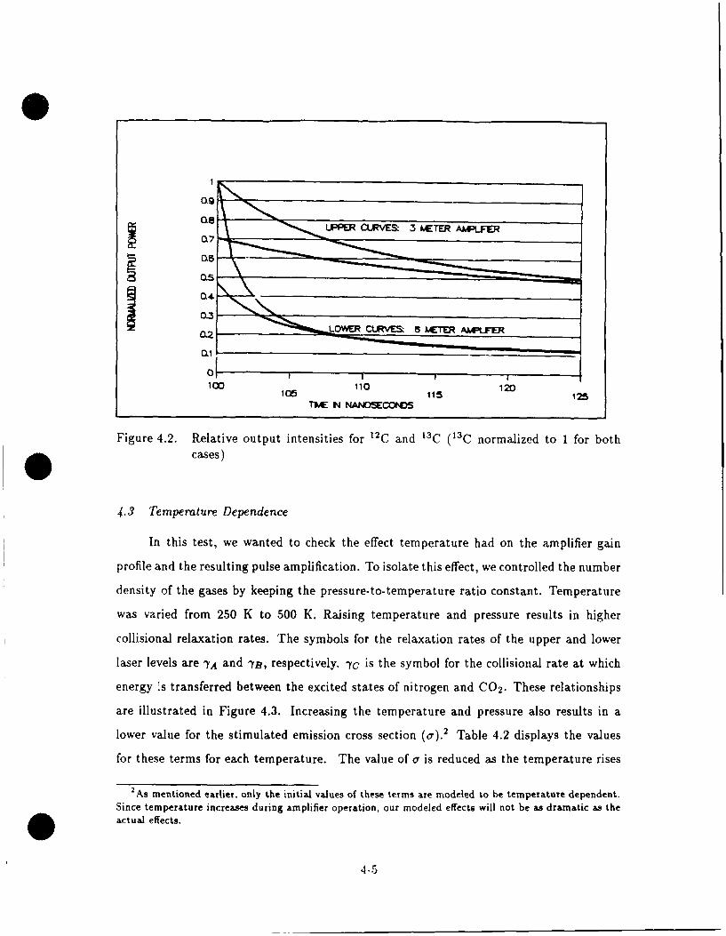
OL

0.4

0.2 LOWER CUMM 6 METER AAILFER

01100 110 120105 115 125

TME N NANOSCONDS

Figure 4.2. Relative output intensities for 12C and 13 C ( 1 3 C normalized to 1 for bothcases)

4.3 Temperature Dependence

In this test, we wanted to check the effect temperature had on the amplifier gain

profile and the resulting pulse amplification. To isolate this effect, we controlled the number

density of the gases by keeping the pressure-to-temperature ratio constant. Temperature

was varied from 250 K to 500 K. Raising temperature and pressure results in higher

collisional relaxation rates. The symbols for the relaxation rates of the upper and lower

laser levels are -YA and 7y, respectively. y¢ is the symbol for the collisional rate at which

energy 's transferred between the excited states of nitrogen and CO 2 . These relationships

are illustrated in Figure 4.3. Increasing the temperature and pressure also results in a

lower value for the stimulated emission cross section (a).2 Table 4.2 displays the values

for these terms for each temperature. The value of a is reduced as the temperature rises

2 As mentioned earlier, only the initial values of these terms are modeled to be temperature dependent.

Since temperature increases during amplifier operation, our modeled effects will not be as dramatic as theactual effects.

4-5

(b) (a) (c)

050 N, N,

200

040 20c001 V=l

030 Nb

100020

010

000

(VI) (V2) ("3) V= 0

Carbon Dioxide Nitrogen

Figure 4.3. Diagram of the kinetic relationships in a four-level CO 2 laser model

for two reasons. First, F,(j=l9 ) decreases with increasing temperature and, second, AvP

increases. Because o gets smaller, the initial gain in the amplifier falls off.

The data in Table 4.2 was calculated using Melan(on's temperature model and shows

that temperature most significantly affects 7B.(1 3 ) As a result, the population inversion

incr"-es faster for higher temperatures. The increasing slopes of the gain curves in Fig-

ures 4.4 and 4.5 illustrate this effect. It is also evident in Figure reffigure29a that even

though the initial slope of the gain curve is steeper for higher temperature, the curve peaks

out earlier. The data in Table 4.2 indicates that this effect is due to the changes in the

kinetic rates that affect the upper lasing level, YA and yc. Increasing temperature increases

both rates. However, over the temperature range, 7,A changes by a factor of 9, while yc

changes by a factor of about 5.7. Thus, the population inversion grows at a progressively

4-6

0Table 4.2. Parameters affected during the temperature dependence test

Temp (K) YA(S - ') -YB(.- 1 ) co,(s- 1 ) 77C,,(s - , a(m 2 ) GAINo(%/m)250 .0005 .0098 .0100 .0110 9.50 E-24 -01.11300 .0010 .0246 .0158 .0174 8.32 E-24 -03.54350 .0017 .0492 .0233 .0256 7.31 E-24 -07.79400 .0025 .0849 .0325 .0358 6.45 E-24 -13.62450 .0035 .1325 .0437 .0480 5.73 E-24 -20.51500 .0046 .1924 .0568 .0625 5.13 E-24 -27.84

slower rate.

The data has been displayed on two graphs for two separate comparisons, one between

the effects o' temperature on gain development, the other between the gain depletion at

the beginning and the end of the amplifier. It should be kept in mind that prior to the

arrival of the input pulse (t = 330 ns) the gain profile is uniform across the amplifier. In

the first comparison, we noted that increasing kinetic rates lead to faster gain development,

including earlier level-off. Higher kinetic rates also result in quicker recovery of the gain

after the pulse has passed through the amplifier. The second comparison simply illustrates

the severity of the gain depletion in the last cell.

The output pulses for the first three temperatures are shown in Figure 4.6. Despite

starting at smaller gain levels, higher temperatures produced significantly higher gain

profiles. Thus, the output pulses had higher peaks for higher temperatures. There were

also indications of more pulse narrowing. For higher temperatures, the peaks occurred

earlier in time and the pulse width between the half-max points was narrower.

However, for temperatures beyond 400 K, these trends were reversed. As shown in

Figure 4.7 the pulses had lower peaks, the peaks occurred later in time, and the pulses

grew wider rather than narrower. Beyond 400 K, the gain leveled off at progressively

lower levels, resulting in less rapid pulse growth and a lower peak. Because the pulse grew

less rapidly, the rate of change in gain was smaller. Higher kinetic rates, forcing a higher

population inversion, also caused the gain to drop off more slowly. With higher gain for

4-7

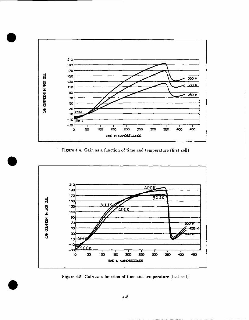
210

190 .oN

170

150

130K

110 300 K

70

70 j250 K

50: 0

10 266K

-10

0 50 100 150 200 250 300 350 400 450

TE IN NANOSECDS

Figure 4.4. Gain as a function of time and temperature (first cell)

210

90 -

170 509 150

130 40

z 1109070 S

-10

-300 s0 100 150 200 250 300 350 400 450

TbIE IN NAN~OSECONDS

Figure 4.5. Gain as a function of time and temperature (last cell)

4-8

580 350 K

48

290 20K

232

116

586z

330 3 45 350 3W0 3M 3335 48 M5 -T/35

ThE N NA1NO5EC0IC

Figure 4.6. Output pulse narrowing for increasing temperatures

;590

5W0

515

344 W 3;4 35 352 3 610 5 360

TE N NANOSEQCS

Figure 4.7. Output power. peaks for increasing temperature

4-9

later segments of the input pulse, the output plse was broader and had a peak that was

moved forward in time.

4.4 Amplification with ASE Effects

The last test in this chapter examined the effects of ASE in the presence of gas

kinetics. From previous analysis, we knew that ASE effects were noticeable in long, wide

amplifiers with relatively high gain profiles. Also, it takes over 150 nanoseconds for both

the population inversion and the ASE intensity to grow to desired levels. So, to evaluate

the effects of ASE, we used an eight-meter amplifier with a diameter of five centimeters.

The gas mix used was a 10:10:80 mix of C0 2 , N2 , and He at 300 K and one atmosphere

of pressure. Also, the pump duration was fixed at 100 nanoseconds. With this set-up we

performed three model runs.

In our first run, we used windows without anti-reflective coating and a very high

pump efficiency (40%). 3 For the second run, we reduced the reflectivity of the windows

from 4% down to 1% and performed runs with pump efficiencies of 25, 30, and 35 percent.

Leaving the pump efficiency at 35%, in our third run, we varied the reflectivity of the

windows from 1% down to 0.01%.

Though the gas mix and the amplifier diameter were fairly standard, our first run

showed that ASE could significantly affect the gain profile in less than 200 nanoseconds.

Figure 4.8 shows that the ASE output and its effect on amplifier gain are very similar to

the operation of a gain-switched oscillator. Looking at the tail of the ASE pulse, we found

that our results concurred with Vereyen's conclusion that once ASE reaches saturation

intensity, "further pumping of the amplifier is futile; spontaneous emission extracts the

energy from the inversion as fast as the pumping agent can create it" (24:183).

In the second run, we found that despite reducing the reflectivity from four percent

down to one percent, ASE was still able to saturate the amplifier. Figures 4.9 and 4.10

show that lowering the pump efficiency will delay the saturation and slightly reduce the

magnitude of the ASE output pulse.

3In our model, pump efficiency refers to the percent of N2 molecules that will transition to the v 1excited state.

4-10

180

IS

140120

4" 100,~o

40 \ZZffASE

-S I I I I I I I I

0 50 100 150 20 20 3W 50 400 450

TME N NAIOSECA14DS

Figure 4.8. Gain evolution and ASE output as functions of time

In the third run, we found that reducing the reflectivity has results similar to reducing

the pump el'fcieitcy. Fgure 4.11 shows that output pulse is delayed more and more as the

reflectivity is reduced. In addition, the magnitude of the output pulse intensity falls off for

smaller reflectivities.

Although our approximation for ASE output is conservative, these examples illustrate

the limitations ASE imposes on amplifier designs. All of these examples have indicated

that for efficient amplification, an input pulse must enter the amplifier before ASE reaches

saturation intensity. This timing is made easier if the window reflectivity is reduced and

amplifier gain is limited. The amplifier gain can be limited by reducing the pump intensity,

altering the gas mix, or coordinated timing of the oscillator and amplifier pumps. To allow

this timing, our model allows the amplifier pump to be delayed relative to the oscillator

pump.

4-11

170

_ 130110

70 35 PCT50

-30 PCT30

-10 1 I I I I II

0 50 150 20 250 3M 350 4

TWE NJ NAM)SEC0ICS

Figure 4.9. Gain as a function of time and pump efficiency under the influence of ASE

90

so80-

70

50

40-

201

10

2M 20 200 0 3M 0 : 340MhE N NAhOSECONiCS

Figure 4.10. ASE outputs for various purmp efficiencies

4-12

70I S50

40

n0 2;0 1 2 O220 250 00 340

TME N' NANOISE0CON

Figure 4.11. ASE outputs for various window reflectivities

4.5 Summary

In this chapter we have examined many aspects of our amplifier model to confirm the

soundness of the combination of this amplifier model with a validated gas kinetics model.

We established tbht because gain changes due to gas kinetics will be small, a time step of

one nanosecond will be a good starting point for any amplifier analysis. Smaller time steps

will be required when other factors result in large rates of gain reduction. These factors

include amplifier length, gain, and input intensity. The next two tests analyzed the isotope

and temperature parameters. The results were consistent with prediction. Finally, in the

last section, we verified that the model had consistent results for ASE output involving

gain profiles established by pumping and gas kinetics. Though it is not widely discussed

in the literature, it appears that ASE is an important design consideration for large CO 2

amplifiers even though the A 21 value for CO 2 is very small.

4-13

V. Conclusions and Rcomrn endations

We have developed and validated a computer simulation of a CO 2 laser amplifier for

uL2 on IBM-compatible personal computers. It allows the input of square pulses as well as

pulses generated with a typical laser oscillator. The other input variables are listed below:

1. Length and aperture diameter.

2. Gas mix formed with N2, He, H, H2 0, and either 2 C0 2 or 13 C0 2.

3. Gas pressure and initial temperature.

4. Pump pulse shape, duration, and efficiency.

5. Time step/amplifier divisions.

6. Loss terms for absorption and window transmissivity.

The user can also choose to model amplification with or without gas kinetics and with or

without ASE consideration. The ability to run the model without the last two parameters

has been added for instructional purposes rather than for actual amplifier design.

The model's accuracy depends on the rate at which the gain is reduced from one time

step to the next as the pulse propagates through any section of the amplifier. Higher rates

of gain reduction are caused by higher pulse intensities and characteristically occur at the

end of the amplifier. These higher rates result in larger errors in pulse shape and energy

gain. Kinetics also play a role in changing the gain, but we have found that using one

nanosecond time steps virtually eliminates this factor as a potential error source. Error

trends for increases in pulse intensity, amplifier length, and amplifier gain were discussed

in Chapter 3 and displayed in Figure 3.2. When using Figure 3.2 as a guideline, one should

keep in mind that these are maximized errors for overall energy gain, and that pulse shape

errors will be significantly smaller.

Several improvements to the model are possible and recommended for follow-on re-

search. We will discuss four possibilities here. First, to improve the accuracy and extend

the analysis capability, the model should be codr ' for use on a mainframe computer. This

will allow time steps much shorter than one nanosecond and hundreds rather than tens

5-I

of amplifier divisions. Until a version is available on a mainframe, long amplifiers may be

modeled using the detailed method described at the end of Appendix A. The second rec-

ommendation is to model the relaxation of the rotational levels as well as the vibrational

levels. The third improvement does not necessarily require a mainframe for application.

This improvement would be to increase the amplifier efficiency by allowing one of the win-

dows to be totally reflecting and create a double-pass amplifier. Lastly, we recommend

further work in the modeling of ASE. The ASE model requires a better approximation

for the amplification of the entire band of ASE frequencies. Also, the results should be

compared with experimental results for validation and error assessment.

5-2

Appendix A. Notes to User

This appendix outlines the use of this CO 2 amplifier model. It is divided into six

sections. The first section provides general guidance and should be read before actually

running the program. The following four sections describe the "filed-pulse" routine, the

"'square-pulse" routine, the output displays, and creating output data files. In the last

section, we examine a method that can be used to circumvent the constraints imposed by

the limited memory of personal computers.

A.1 General Guidance

To achieve reasonable results, the user should keep several things in mind. In this

section, time constraints, memory constraints, and parameter limits will be discussed.

A.1.1 Time Step Effect on Run Time and Memory Limits. Smaller time steps lead

to smaller relative errors. However, small time steps lead to longer run times and may

cause the memory limit to be exceeded. Smaller time steps cause longer run times for two

reasons, both of which are related to the number of integrations that will be done during

the simulation run. First, a smaller time step breaks the period of interest into more time

increments. Second, it divides the amplifier into more cells. One integration is done per

cell per time increment, so the number of integrations for a given time step and amplifier

length is given by

Integrations = (tmax)/(hi) x (Length)/(hi x tcav x c) (A.1)

where tcav is the base time unit, tmax is the period of interest in base time units, hi is

the time step (fraction of the base time unit), and cLight is the speed of light. Sample

integration values appear in Table A.1. Notice that when the time step is cut in half, the

number of cells doubles, but the number of integrations quadruples. The time steps used

to divide the amplifier into an even number of cells were calculated as follows:

hi = (length)/(tcav)(c)(nu tmber of cells) (A.2)

A-I

Table A.1. Influence of time step on the number of program integrations. Length = 2meters, tcav = 10 nanoseconds, tmax = 20

time step Cells Integrations,1334 5 750.1112 6 10800953 7 1470

,0834 8 1920.0741 9 2430.0667 10 3000

.0606 11 3630

After each time step change, the number of integrations to be done is recalculated and

displayed on the input screen. The user should keep in mind that the model executes

approximately 3200 integrations per minute. 1

For each integration, seventeen different variables are stored in memory for interme-

diate calculations and output displays. Since the amount of memory available is related

to Lhe number of integrations, it is also affected by time step reductions. Another reason

memory available is sensitive to time step changes, is that eleven of the seventeen variables

stored in memory are stored in two-dimensional arrays. After each change is made to the

time step, the amplifier length, or the maximum run time, the program will display the

user's available memory.

The factors that require the use of small step sizes and large volumes of memory

also lead to high output intensity. For sound results, small time steps are required to

describe amplification in the presence of any of the following: a long amplifier (L > 5

meters), a large input intensity ( I > 5 MW/cm2 , or a high gain amplifier (g > 150

percent/meter). Guidelines for time step selection are as follows. (1) Start with a time

step of one nanosecond. This value will keep up with any changes in gain due to gas

kinetics. (2) The maximum gain change in the last cell will be displayed on the output

screen following each run. As this value is minimized, so is the relative error. (3) While an

'This speed is an averaged value using a computer with an 80287-10 math coprocessor.

A-2

input pulse is propagating, if the gain coefficient in the last cell falls to a value less than

the "loss-per-unit-length" term (a), then a smaller time step is recommended.

A.1.2 Parameter Limits. The following parameter limits are estimates. They are

provided to help the user obtain accurate and valid results from this amplifier model.

Gas Mix The gas percentages should add up to 100 percent and there must be some

percentage of CO 2. !n the filed-pulse routine, the CO 2 isotope will be the same as

the one used to generate the file during the oscillator run. Mixing isotopes between

the oscillator and the amplifier would result in no amplification whatsoever.

Temperature The temperature-dependent collisional relaxation rates in this model are

valid for temperatures > 200 K.

Pressure The model is valid only for pressures where the lineshape is Lorentzian. So, the

pressure should be greater than 0.015 atmospheres.

Pump Efficiency Reasonable pump efficiencies include values up to 20 percent.

Loss Per Unit Length (a) Values for a vary with the gas mix and typically range be-

tween 2 and 4 percent.

Reflectivity Values for reflectivity can range from fou, pt icent down to less than one

hundredth of one percent (with anti-reflective coatings). For amplifiers with beveled

ends (angled windows) the reflectivity can be set to zero.

Length The amplifier length is limited by the available memory and the patience of the

user. Longer amplifiers require smaller step sizes, longer run times and, depending

on the time step used, can cause data storage problems.

Diameter There are no model limits on the diameter of the amplifier, however, the user

should keep in mind that the smaller the diameter for a given input amplitude, the

higher the intensity. High intensities require smaller time steps to keep the relative

error within reasonable limits. So, smaller diameters can lead to problems similar to

those encountered with long length inputs.

Oscillator Volume/Input Amplitude These inputs also determine the intensity of the

input pulse. For the "filed-pulse" routine, the oscillator volume parameter is used in

A-3

the conversion from megawatts per liter to photons per cubic meter. A typical value

is one liter. For the square-pulse routine, the value for input amplitude is limited

only by the resulting intensity. The input screen display- and updates the intensity

for changes in diameter as well as input amplitude. Smaller input amplitudes and/or

larger diameters are recommended to keep the intensity under 10 MW/cm2.

Kinetics The user has an option to allow the population inversion to be developed by gas

kinetics or to "turn off" the gas kinetics and let only the incoming pulse affect the

inversion. If the kinetics are turned off, the user must input a value for the initial

gain coefficient. Typical values range from 50 to 200 percent per meter.

Amplified Spontaneous Emissions For CO 2 amplifiers less than two meters long, ASE

is not a significant loss factor unless the gain is over 300 percent per meter. However,

as amplifiers get longer, ASE becomes an important factor at lower values of gain.

For example, ASE can reach saturation intensity in a six meter amplifier with a gain

of only 120 percent per meter.

A.2 Filed-Pulse Routine

The filed-pulse routine begins during the output portion of Stone's oscillator model.

Here, files are created to store parameter input data and power output data. Files must

be created using a "file step" of one. That is, each data point should be saved. This is

because the amplifier uses one time step at a time and must have an input value for each

time step.

Most oscillator runs use two time steps. With this "change-time-step" option, the

first time step (hi) is for the pulse portion of the output and the second, larger time step

(h2) is for the linear portion of the output, The amplifier model can only use one time

step because the time step defines the number of amplifier divisions. Data saved using the

"change-time-step" option can be used as an input to the amplifier model only if the value

for h2 is divisible by hl. In this way, hl will be the amplifier's time step and extra input

values will be calculated by simple linear interpolation. For example, if hl is 0.1 and h2 is

2.0 then 20 input values have to be calculated between each h2 increment.

"k -4

Ideally, the time step used in the oscillator will be small enough to provide accurate

amplifier results. If not, the user can cut his time step in half. Again, linear interpolation

will be used to calculate the additional input values. The time step can be cut in half as

many times as memory will permit.

.4.3 Square-Pulse Routine

With respect to time steps, the square-pulse routine is more flexible than the filed-

pulse routine. The user can choose any time step or number of cell divisions without

consideration for a file of input values. Though this routine allows only square input

pulses, the user is in control of pulse amplitude and pulse duration.

When adjusting the start and stop times for the square input pulse, the user will

see on the screen display that the total run time also changes. As an explanation for this

change consider an amplifier divided into five cells. Each cell has a length of one time step.

If the pulse starts at the first time step and ends on the tenth, it takes a total of fifteen

time steps for the entire pulse to exit the amplifier. To allow the pulse to completely pass

through the amplifier, the total run time must extend at least five time units past the stop

time of the pulse.

Another facet of the square-pulse routine is a comparison between the model's en-

ergy gain and the energy gain derived using Frantz and Nod',ik's closed form solution.

Originally, this comparison was used for validation purposes, but it has been left in the

model to give the user a feel for the model's accuracy. To see this comparison, the user

must set up the following conditions:

1. Turn off kinetics.

2. Set reflectivity to zero.

3. Set ASE value to "n."

A.4 Screen Displays

While the program is running, the screen will display the elapsed time in seconds,

the amount of work completed in percent, and the current time step. A second row of

A-5

data displays updated values for the ASE output, the pulse output, and the gain in a

predetermined cell. The user will be given an option as to which cell is to be monitored.

At the completion of the run, another set of numbers will be listed on the screen. This set

of numbers represents the gain in each cell across the amplifier.

Following the completion of the run the user has a choice of two output data displays.

The first display shows the time variation of gas populations (N 2 , C0 2(001), and C0 2(100))

along with the power input (Pin), the power output (Pout), and the gain in a predetermined

amplifier cell (Gain#). The second display trades the gas populations for columns showing

the time variation of the energy output, the ASE output, and the gain in the first amplifier

cell.

The displays are basically self-explanatory. However, one point that should be made

clear deals with the lag time between a pulse input unit and its corresponding output.

To compare an input unit to its output, the screen display should be displayed with an

increment of one. Then to locate the output for an specific input, the user must count

down a number of time steps equal to the number of amplifier divisions.' Understanding

this time lag makes it easier to see how a pulse's shape is altered after passing through an

amplifier.

A.5 Storing Files

Once the run is complete, the user has three options. He can skip between the output

screens at will, he can start over, or he can choose to make data files for future use. Data

files can be made for the following outpiits: populations, energy, ASE, gain, and power.

For each data file created, a supplemental file is also created. This file contains various

information about the particular amplifier run.

Data is stored in a simple format. Each line of data begins with its time reference

and is followed by the data element. The files have suffixes that let the user know which

data set is in which file. All of the data files have one data element except for the power

data file. It has elements for both the input and output power.

2 Each amplifier division corresponds to one time unit.

A-6

A.6 Overcoming Memory Limitations

Modeling long amplifiers not only requires smaller time steps and very long run

times, it can also cause data storage problems. Personal computers have limitations on the

amount of random access memory available for applications programs. In our program,

storage of output array data consumes the most memory. The sizes of these arrays depend

on amplifier length, time step, and maximum run time. Maximum run time is important

because data is stored for each time step. Depending on the gas kinetics, the amplifier

might require a relatively long period of time to establish its high gain profile. In such a

case, memory might be insufficient to even begin the run.

To overcome this limitation, the model can be used to generate the output data for the

amplifier one section at a time. For example, a fifteen-meter amplifier might be modeled as

three consecutive five-meter amplifiers or five consecutive three-meter amplifiers. The only

designs where this technique is applicable are those amplifiers with anti-reflective coatings

on its windows. There are two reasons for this limitation. First, ASE calculations would

be completely unreasonable. Second, there would be additional window losses because

each section would add two more windows to the overall model. We use only one input

parameter to describe the reflectivity of both amplifier windows. So, even if we set the

reflectivity to zero for all but the first and last section, we will still have two extra window

losses.

The first test accomplished was to compare the output of an entire fifteen-meter

amplifier to one that had been cut into three sections. Using zero reflectivity and identical

time steps, the outputs agreed to six decimal places. Next, we divided the whole amplifier

into 20 cells and the amplifier made of sections into 60 cells (20 cells per section). Figure A.1

compares the outputs for these two cases. Curve A represents the 20 cell amplifiers output.

Curve B is sharper because its leading edge experiences slightly higher gain. As mentioned

earlier, increasing the number of cells allows the kinetics to go through more iterations

and develop higher gain at the end of the amplifier. Higher gain allows more energy to be

extracted sooner, so curve B falls off faster than curve A. This more refined pulse shape

shows the advantage of using a series of short amplifiers to model one very long one.

A-7

130

120

0 110

90

160 180 200 220 240 260170 TI 0 N N 9 0NDS 230 250 270

Figure A.1. Output pulse calculated using (A) 20 cells and (B) 60 cells

0A-8

Appendix B. Derivation of Factorl

The output from Stone's oscillator model has units of megawatts per liter of oscillator

volume. For consistency, the input file generated during the square pulse routine also has

these units. This amplifier uses photons per cubic meter as its base unit. To get from

megawatts/liter to photons/meter3 , the first step is to multiply by the oscillator volume to

arrive at megawatts. Then Factorl is used to complete the conversion. Factorl considers

the time step used (tcav x hi), the cross-sectional area of the amplifier (Area), and the

frequency of the output beam (v).

The time step determines the energy contained in each power unit and how much

linear distance the power unit will occupy in the amplifier: x = c x tcav x hi. The

cross-sectional area completes the calculation for the volume filled by the photons of the

power unit. The frequency determines the energy per photon by the expression E = hv,

where h iz P!anck's constant.

Step by step, Factor1 is given by the following:

a Megawatts to watts - (MW) x(1000000)

, Watts to Photons/second - (W) -(hv)

e Photons/second to photons - (photons/second) x (tcav x hl)

9 Photons to photons/m 3 - (photons) + (Area X c x tcav x hi)

When simplified the equation for Factorl is:

1000000Factorl 1 (B.1)

(hv)(c)(Area)

B-I

Appendix C. ASE Analytic Solution

In this appendix, we will summarize our analysis into the reason why our results

for ASE gain limits were consistently higher than those calculated with a basic analytical

equation.

C.1 Basic Equation

Both Milonni and Verdeyen described the condition where ASE reaches saturation

intensity (14, 24:400,183). Their derivations are different, but they arrive at similar results

for an expression for the maximum permissible gain in an amplifier. Milonni and Verdeyen

begin with the equation for radiation traveling in the positive z direction:

A - 21 hvQ) N2 (C.1)

where N2 is the population of the upper level and g is the gain coefficient. By allowing 1(z)

to be the saturation intensity for the amplifier, they arrive at an intermediate solution:

e9 L - 1 1/A 21 4r (N 2 - N1 (C.2)72 _Q N2 )

Following the three assumptions described below, they arrive at

16L 2 (C.3)- d=--(C3

as the equation limiting the amplifier's gain, length, and diameter. When the left-hand

side of this equation becomes greater than the right-hand side, ASE will significantly affcct

the operation of the amplifier.

C.2 Analysis of Assumptions

The three assumptions used to arrive at this simple equation are not used in our

model. Therefore, we examined these assumptions to determine the reason our amplifier

C-1

model required significantly higher values for g to cause ASE to reach saturation intensity.

The three assumptions are:

N21. (- N 1.

(N2 - NI)

Area 16L 2

L 2 d2

1/A 213. = 1.T-2

Using typical values for the populations of the upper and lower laser levels we found

that as the gain increased, the validity of the first assumption also increased. Table C.1

shows this trend. Because this assumption is valid for high values for the gain coefficient,

Table C.1. Relationship between gain coefficient and the ratio N 2 /(N 2 - NI)g (%) Ratio

5 2.92

10 1.96

20 1.4840 1.2480 1.12160 1.06

it does not explain the difference between the model's results and the analytic equation.

Next, we looked at the approximation for solid angle, Area/L 2 . While this value is

adequate for positions close to the beginning of the amplifier, it underestimates all val-

ues closer to the end. Table C.2 shows how the solid angle varies for positions in an

amplifier and indicates the magnitude of the error by tabulating values for (Integral Solu-

tion/Approximation]. (The positions are based on a one-meter amplifier.) Equation C.3

shows that gain is limited by the reciprocal of the solid angle. Thus, these large differences

between the actual and the approximate values for solid angle indicate that the actual

value for the gain limit is higher than that given by Equation C.3.

This is only a partial explanation for our model's results. Though the solid angles

are larger, the actual contribution to ASE output is still rather small for positions near the

C-2

Table C.2. Comparison between solid angle approximation and an integral solution

Position (m) Appoximation IntegralAppror.

0.0 0.00196 0.00196 1.000.1 0.00196 0.00242 1.230.2 0.00196 0.00306 1.560.3 0.00196 0.00400 2.030.4 0.00196 0.00544 2.770.5 0.00196 0.00784 3.990.6 0.00196 0.01224 6.230.7 0.00196 0.02170 11.10.8 0.00196 0.04852 24.70.9 0.00196 0.18760 95.5

end of the amplifier. Photons emitted at these positions are amplified over only a short

distance, so their ability to extract energy is very limited.

The best explanation for our model's results was found upon examining the last

assumption. In CO 2 lasers, the lifetime of the upper vibrational level depends not only

on its slow spontaneous emission rate, but also on a high rate of collisional relaxation.

Therefore, the lifetime of the upper state, (r 2), is far shorter than 1/A21. This makes the

value for 11A much greater than one and explains why our value for ttL gain allowingT-2

ASE to reach saturation intensity is higher thani the gain calculated with Equation C.3.

C-3

0 Appendix D. ASE Variations Due to Large Solid Angles

In addition to causitg timing errors for input pulse reflections, fractional cells also

played a role in causing asymmetric ASE outputs. In our model, the fractional cell is

always the last cell. Because of this, the solid angle subtended in the positive direction at

the final cell is always greater than the solid angle subtended in the negative direction at

the first cell. Therefore, if a fractional cell exists, the ASE outputs will never be perfectly

symmetric.

Until the gain in the fractional cell is depleted, the ASE output from the positive end

of the amplifier will have a larger value. ASE is a function of A21, population of the upper

vibrational level, cell length, and solid angle. To compare the outputs at the two ends, we

need only consider the last two. For example, if we have a cell length of 30 centimeters and

a diameter of 5 centimeters, our model calculates Ql/4r to be 0.0068. If the fractional cell

is only two centimeters long, its value for Ql/47r is .3143. Including the length difference,

the amount of ASE that leaves the last cell is triple the amount that leaves the first cell.

While this causes a loss in symmetry, it actually makes our approximate ASE output value

closer to the theoretical value.

In general, the shorter the cells are, the higher the value for ASE output will be. This

is true with or without fractional cells. The large values for S/47r occur only when measured

at distances within a diameter's length from the end of the cavity and the maximum

value for f2/4ir is only 0.5. So, for the last few centimeters of the amplifier, our model

underestimates the ASE output. The amount of the error increases for longer cell lengths.

For cell lengths smaller than 30 centimenters (time steps < one nanosecond) the error

is insignificant when compared to the ASE output for the entire amplifier. Additionally,

because of our line shape approximation, we still have a conservative approximation for

the ASE output.

0Dl-I

Bibliography

1. Allen, L. and G. I. Peters. "Amplified Spontaneous Emission and External SignalAmplification in an Inverted Medium," Physical Review A, 8: 2031-2046 (October1973).

2. Chow, Weng W. "Amplified Spontaneous Emission Effects in Laser Amplifiers," SPIEProceedings, 1045: 139-147 (1989).

3. Comly, J. C. Jr. et al. "Discharge and Kinetics Modeling in Electron-Beam ControlledCO 2 Laser Amplifiers," IEEE Journal of Quantum Electronics, QE-17: 1786-1798(September 1981).

4. Douglas-Hamilton, D. H1. et al. Carbon Dioxide Electric Discharge Laser KineticsHandbook. Technical Report AFWL-TR-74-216. AVCO Everett Research Laborato-ries, Everett MA, June 1974 (AD-A008 650).

5. Frantz, Lee M. and John S. Nodvik. "Theory of Pulse Propagation in a Laser Ampli-fier," Journal of Applied Physics, 34: 2346-2349 (1963).

6. Frey, R. W. et al. "Laser Imaging Radar Sensor (LIRS)," SPIE Proceedings, 500: 2-9(1984).

7. Gilbert, J. et al. "Dynamics of the CO 2 Atmospheric Pressure Laser with TransversePulse Excitation," Canadian Journal of Physics, 50: 2523-2535 (October 1972).

8. Glazenkov, V. M. et al. "Experimental Determination of the Parameters ofVibrational-Rotational Transitions in Isotopic Forms of CO 2 Molecules," Soviet Jour-nal of Quantum Electronics, 18: 534-536 (April 1988).

9. Harney, R. C. "Comparison of Techniques for Long-Range Laser Ranging," SPIEProceedings, 783: 91-100 (1987).

10. Harney, R. C. "Military Applications of Coherent Infrared Radar,"SPIE Proceedings,300: 2-11 (1981).

11. Manes, K. R. and H. J. Seguin. "Analysis of the CO 2TEA Laser," Journal of AppliedPhysics, 43: 5073-5078 (December 1972).

12. McQuillan, A. K. and A. I. Carswell. "Spatially Resolved Gain Measurements in a

CO 2 Amplifier," Canadian Journal of Physics, 50: 769-777 (1972).

13. Melangon, T. B. A Model of Temperature Effects in Pulsed and Continuous WaveC0 2 Laser Models and Optimization Using Response Surface Methodology. MS Thesis(work in progress), AFIT/GSO-89D. School of Engineering, Air Force Institute ofTechnology, Wright- Patterson AFB, Ohio, December 1989.

14. Milonni, Peter W. and Joseph H. Eberly. Lasers. New York: John Wiley and Sons,1988.

15. Pace, Paul, et al. "Frequency-Stabilized Transversely Excited Atmospheric (TEA)CO 2 Lasers for Coherent Infrared Radar Systems," SPIE Proceedings, 300: 148-152(1981).

BIB-1

16. Patel, C. K. N. "CO 2 Lasers," Scientific American: 23-34 (August, 1968).

17. Pressley, Robert J. CRC Handbook of Lasers. Cleveland, 011: The Chemical Rubber

Company, 1971.

18. Reilly, James P. "CO 2 Frequency Stable Amplifier Assessment," SPIE Proceedings,

783: 60-68 (1987).

19. Rooth, R. A., J. A. van der Pol, and E. H. Hasselhoff. "Intramode and Fermi Re-

laxation in C0 2 , Their Influence on Multiple-Pass, Short-Pulse Energy Extraction,"

Applied Physics B, 42: 103-110 (September 1986).

20. Schulz-Dubois, E. 0. "Pulse Sharpening and Gain Saturation in Traveling-Wave

Masers," Bell Systems Technical Journal, 3: 625-658 (March 1964).

21. Slater, Philip N. Remote Sensing. Reading, MA: Addison-Wesley Publishing, 1980.

22. Stone, David H. Class lecture for Physics 520, Introduction to Laser Physics. Schoolof Engineering, Air Force Institute of Technology (AU), Wright-Patterson AFB OH,Fall 1988.

23. Tsunawaki, Y. "Copper and Molybdenum Mirrors for High Power TEA CO 2 Lasers,"

SPIE Proceedings, 1019: 414-415 (1988).

24. Verdeyen, Joseph. Laser Electronics. Englewood Cliffs, NJ: Prentice-Hall, 1981.

25. Witteman, W. J.The C0 2 Laser. Heidlberg, Germany: Springer-Verlag Berlin, 1987.

26. Yoder, M. J. et al. "Development of CO 2 Laser Amplifiers for Radar Applications."

SPIE Proceedings, 709: 46-51 (1986).

BIB-2

Vita

Frank Patrick Gallagher II Ile

in 1980 Wnoved to Colorado Springs,

Colorado to attend the United States Air Force Academy. In 1985, lie received thc- degree

of Bachelor of Science in Civil Engineering. After graduation, he entered active duty in

the Air Force and served as an Orbital Analysis Officer in the Space Surveillance Center at

Cheyenne Mountain Air Force Base. In May of 1988, he entered the School of Engineering,

Air Force Institute of Technology at Wright Patterson Air Force Base, Ohio.

VITA-i

UNCL.ASSIFIED

SECURITY CLASSIFICATION OF THIS PAGEj Form Approved

REPORT DOCUMENTATION PAGE OMB No. 0704-0188

REPORT SECURITY CLASSIFICATION lb. RESTRICTIVE MARKINGSUNCLASSIFIED

2.a. ".URITY CLASSIFICATION AUTHORITY 3. DISTRIBUTION/AVAILABILITY OF REPORTApproved for public release;

2b. DECLASSIFICATION/DOWNGRADING SCHEDULE distribution unlimited

4. PERFORMING ORGANIZATION REPORT NUMBER(S) 5. MONITORING ORGANIZATION REPORT NUMBER(S)

AFIT/GSO/ENP/ENS/89D- 2

6a. NAME OF PERFORMING ORGANIZATION 6b. OFFICE SYMBOL 7a. NAME OF MONITORING ORGANIZATION(If applicable)

School of Engineering AFIT/7NP/EN3

6c. ADDRESS (City, State, and ZIP Code) 7b. ADDRESS (City, State, and ZIP Code)

Air Force Institute of TechnologyWright-Patterson AFB, OH 45433-6583

8a. NAME OF FUNDING/SPONSORING 8b. OFFICE SYMBOL 9. PROCUREMENT INSTRUMENT IDENTIFICATION NUMBERORGANIZATION (If applicable)

WRDC AARI

8c. ADDRESS (City, State, and ZIP Code) 10. SOURCE OF FUNDING NUMBERSPROGRAM PROJECT TASK WORK UNIT

Wright-Patterson AFB, OH 45433 ELEMENT NO. NO. NO ACCESSION NO.

11. TITLE (Include Security Classification)

NUMEPIC MODEL OF A CO 2 LASER AMPLIFIER (U NCLASSIFIF )

PERSONAL AUTHOR(S)Frank P. Gallagher, B.S., Captain, USAF

13a. TYPE OF REPORT 13b. TIME COVERED 14. DATE OF REPORT (Year, Month, Day) 15. PAGE COUNTPMS Thesis IFROM ____TO _ __1989 DECEMBEP Pfl

16. SUPPLEMENTARY NOTATION

17. COSATI CODES 18. SUBJECT TERMS (Continue on reverse if necessary and identify by block number)FIELD jGROUP SUB-GROUPFIELD GROUP SUB-GROUP Carbon Dioxide; Laser; Amplifier; Model;

( C3u Amplified Spontaneous Emission19. ABSTRACT (Continue on reverse if necessary and identify by block number)

Thesis Advisor: Dr. David H. StoneAssistant ProfessorDepartment of Engineering Physics

DISTRIBUTION,'AVAILABILITY OF ABSTRACT 21. ABSTRACT SECURITY CLASSIFICATIONUNCLASSIFIED/UNLIMITED 0 SAME AS RPT. C] DTIC USERS UNCLASSIFIED

22a. NtME QF RESPONSIBLE INDIVIDIJAL 22b. P1.P E Wnlvdere 22c. OFFICE SYMBOLuavid 11. Stone, assistant Professor -ENP

DO Form 1473, JUN 86 Previous editions are obsolete. SECURITY CLASSIFICATION OF THIS PAGE

UNCLASSIFIED

UNCLASSIFIED

Abstract

A CO 2 laser amplifier simulation model is developed for use on IBM-compatil,he

per_,onal computers. First, a general laser amplifier is modeled by dividing an aniplific

into separate cells to model both the temporal and spatial dependence of the ampiifiers

gain. The resulting amplification is validated by comparison with a closed-form solution.

Second, losses due to amplified spontaneous emissions (ASE) are investigated and included

in the model. Equations for ASE losses consider both the solid angle of the emissions ard

the reflectivity of the cavity windows. Other reflections are ignored. Third, an existing

numerical model of CO 2 gas kinetics is incorporated. In this kinetics model, temperature-

dep~endent terms are fixed according to initial conditions, and the rotational levels of tiQe

upper CO 2 vibrational sta~e are assumed to be in equilibrium.

The user-friendly model allows designers and students to investigate the amplific:1-

tion of either square input pulses or pulses generated with a laser oscilltor while varyinlg

several input parameters. Among the variable parameters are length, diameter, gas mix.

temperature, pressure, window reflectivity, and pump efficiency.

T'.,CLAES TFIE