Number of Factors

Multiple Linear Regression Viewpoints, 2013, Vol. 39(1) 1

A Comparison of Ten Methods for Determining

the Number of Factors in Exploratory Factor Analysis Robert Pearson Daniel Mundfrom Adam Piccone University of Northern Colorado Eastern Kentucky University Datalogix

The effectiveness of 10 methods for estimating the number of factors were compared. These methods

were the minimum average partial procedure, the likelihood ratio test, the Akaike information criteria

(AIC), the Schwarz information criteria, the common factor and principal component versions of parallel

analysis, the standard error scree test, and the eigenvalues greater than average criterion. Two simulation

studies were conducted. In the first study, the true number of factors, variable-to-factor ratio, level of

communality, and sample size were manipulated. The second study included factor correlations as an

additional experimental variable. Common factor parallel analysis was the most consistently accurate

method across conditions and studies. Neither eigenvalue rule performed well, but the common factor

version was superior. Over almost all conditions, the AIC was either correct or overfactored by one and

might; thus, be a reasonable alternative.

erhaps the most important step when conducting exploratory factor analysis (EFA) is deciding the

number of factors to extract (Zwick & Velicer, 1986). Extracting an incorrect number of factors can

have detrimental consequences on attempts to interpret a rotated factor solution (Fava & Velicer,

1992, 1996; Gorsuch, 1983). Cattell and Vogelmann (1977) describe this step as one of two that can ruin

factor analytic research (the other being inadequate rotation). Many methods have been proposed to

estimate the correct number of factors. The purpose of this study was to expand upon previous research

and examine the performance of several prominent methods under a wide variety of factor structures.

Let m represent the true number of common factors in a factor system. Guttman (1954) proved that

three lower bounds for m can be obtained by examination of the population correlation matrix Σ. The

weakest of these is the number of eigenvalues of Σ that are greater than unity. The strongest of the three

lower bounds is the number of positive eigenvalues of the reduced correlation matrix ΣSMC which is

obtained by replacing the diagonal elements of Σ with each variable’s squared multiple correlation.

Guttman emphasized that the proofs only hold in absence of sampling error.

Kaiser (1960), ignoring Guttman’s emphasis that his bounds only hold in absence of sampling error,

argued that the number of eigenvalues of the observed sample correlation matrix R that are greater than

one (EV-F) should be considered as the number of factors. Kaiser contended that this criterion is

necessary and sufficient for a factor to have positive reliability. Many authors have subsequently observed

that the EV-F rule tends to overestimate the number of factors (Browne, 1968; Gorsuch, 1983, 1997;

Zwick & Velicer, 1986), especially when communalities are small to moderate or the variable-to-factor

ratio is large. In spite of the widespread criticism of its use, the EV-F rule has been and remains the de

facto standard in applied research (Fabrigar, Wegener, MacCallum, & Strahan, 1999; Ford, MacCallum,

& Tait, 1986; Henson & Roberts, 2006; Park, Dailey, & Lemus, 2002). Thompson and Daniel (1996)

suggested that the prevalence of this rule results from it being the default in most statistical packages. A

common factor variation on the EV-F rule is to count the number of eigenvalues of RSMC that are greater

than the average, where RSMC is the sample analogue to ΣSMC. Let EV-R denote this common factor

variant.

Cattell (1966) suggested the scree test, in which the ordered eigenvalues are plotted and m is chosen

such that the final points approximately fit a straight line, where p denotes the number of observed

variables. Methodologists have found the scree test to work well (Cattell & Vogelmann, 1977; Tucker,

Koopman, & Linn, 1969; Zwick & Velicer, 1982). Zwick and Velicer (1986) found the scree test to be

more accurate and less variable than the EV-F rule or Bartlett’s test (discussed later). The traditional scree

test is conducted visually and is; thus, subjective in its application. More recently, regression-based

methods that approximate the tenets of the visual scree test have been developed for the intentions of

objectifying and automating the procedure. Nasser, Benson, and Wisenbaker (2002) found the standard

error scree test (SEscree), proposed by Zoski and Jurs (1996), performed best in a Monte Carlo

comparison of several regression-based scree tests. The SEscree test is conducted by regressing the p

eigenvalues on their ordinal numbers and computing the standard error of estimate. Then in sequence, the

P

Pearson et al.

2 Multiple Linear Regression Viewpoints, 2013, Vol. 39(1)

largest eigenvalue is omitted and the standard error is computed similarly from the remaining eigenvalues

until the standard error is less than some cutoff; for which Zoski and Jurs proposed .

Horn (1965) argued that rather than comparing eigenvalues to unity as suggested by Kaiser (1960), a

better criterion should take into account the degree of sampling variability expected in the elements of the

sample correlation matrix. If an n x p data matrix X is generated such that every element is randomly

generated from the standard normal, the off-diagonal entries of the resulting correlation matrix R = X′X

will deviate from zero. Sampling theory suggests that those deviations will have a mean of zero and

variance inversely related to n. Thus, the p eigenvalues of the random correlation matrix will not all have

a value of unity; rather, half will be greater than one and the other half between 0 and 1 since they must

sum to tr(R) = p. Horn suggested generating multiple random data matrices, each of the same dimensions

as the observed dataset. Then the mean of the simulated first roots should be used as the criterion for the

largest actual eigenvalue, the mean of the second simulated roots the criterion for the second actual

eigenvalue, and so forth. Humphreys and Ilgen (1969) suggested performing this process on the reduced

correlation matrix RSMC and christened the procedure parallel analysis. We will refer to the principal

components and common factor variations of parallel analysis respectively as PA-F and PA-R.

Humphreys and Montanelli (1975) found PA-R to perform quite well, while Zwick and Velicer (1986) in

their seminal simulation study found PA-F to consistently outperform the EV-F rule, the visual scree test,

the Bartlett’s likelihood ratio test, and the minimum average partial method. Rather than using the mean

of the simulated eigenvalues, some authors have advocated using the more conservative 95th percentile

(Cota, Longman, Holden, & Fekken, 1993; Glorfeld, 1995).

Another class of methods for estimating the number of factors is focused on examining the matrix of

residual correlations. Of these, perhaps the most prominent is Velicer’s (1976) minimum average partial

(MAP) approach. He proposed computing the average squared partial correlation after fitting m

components. This computation is done for all candidate models, and the one with the minimum average

partial is retained. Zwick and Velicer (1986) found this method to be accurate under many conditions,

particularly when the ratio of variables to factors is large. When this ratio is small, the MAP method

tended to underestimate the number of components.

Finally, several methods for determining m have been derived for the maximum likelihood (ML)

method of factor extraction. Let F denote the ML discrepancy function, then a likelihood ratio test (LRT)

statistic can be used to test the null hypothesis that the population correlation matrix Σ is that which is

implied by the model with m factors versus the alternative that Σ is any arbitrary positive definite matrix

(sometimes called the saturated model). Bartlett’s statistic (1950, 1951), which uses a modification to the

LRT statistic, approximately follows a chi-square distribution and a formal hypothesis test can thus be

conducted. While the LRT test is statistically appealing, in practice it has been shown to frequently

overfactor, especially when the sample size is large (Gorsuch, 1983; Hakstian, Rogers, & Cattell, 1982;

Zwick & Velicer, 1986). In general, the susceptibility to the influence of sample size is the most

commonly criticized aspect of the LRT method, especially given the formulation of the statistical

hypotheses such that a researcher examining a particular model may perceive greater power as

detrimental.

The maximum likelihood method also enables the use of descriptive measures of model fit. Akaike

(1973) introduced an information criterion, known as AIC, for application to time series models. The

general idea is to measure the fit of a statistical model to observed data via the maximum likelihood fit

function and to incur a penalty for the number of estimated parameters, k. The AIC is thus computed

as -2F + 2k and is a measure of the badness of the fit of a model. For a set of competing models estimated

by maximum likelihood, the one with the smallest AIC is deemed best. The use of AIC specifically for

factor analysis was discussed by Akaike (1987). Schwarz (1978) suggested a Bayesian information

criterion (BIC), also known as Schwarz’s Bayesian criterion (SBC), which is computed in the same

manner as the AIC but replaces the term 2k with the larger penalty of ln(k), the natural log of k.

Although there already exists a considerable amount of literature on methods for determining the

number of factors, much of it is expository in nature (e.g., Fabrigar et al., 1999; Gorsuch, 1983, 1997;

Preacher & MacCallum, 2003). The effectiveness of number-of-factor techniques has often been

demonstrated by applying them to “classic” data sets such as the 24 ability variables of Holzinger and

Swineford (1939) or Emmett’s (1949) nine variables, or deliberately designed “plasmodes” (Cattell &

Number of Factors

Multiple Linear Regression Viewpoints, 2013, Vol. 39(1) 3

Vogelmann, 1977). Monte Carlo simulation has been used to provide empirical evidence for the accuracy

of decision methods, but these studies have been somewhat limited in terms of either the breadth of

examined methods or the variety of conditions in which they were compared. Perhaps the most

comprehensive published simulation to date was conducted by Zwick and Velicer (1986) in which they

studied four PCA-based methods, MAP, parallel analysis, Kaiser’s rule, and the visual scree test, as well

as Bartlett’s LRT chi-square test at three significance levels. They created 6x2x2x2 = 48 population

correlation matrices by varying pattern complexity, number of factors, number of variables, and

component saturation (size of major-component loadings). From every population matrix, five sample

correlation matrices were generated using two sample sizes for a total of 480 sample matrices. Their focus

on principal components methods is an important limitation since many factor analysts favor the common

factor approach. Other empirical studies have often focused on a particular method or class of method.

The purpose of the current study was to provide applied researchers with empirically supported

guidance on how to estimate the number of factors in the initial stages of exploratory factor analysis. To

that end, we utilized Monte Carlo simulation methods to compare the accuracy of 10 decision methods

from three prevalent factoring paradigms: principal components analysis, principal axis factoring, and

maximum likelihood factoring. Data were generated from a wide variety of factor models with extensive

replication. The 10 examined methods were:

• the number of eigenvalues of the full correlation matrix R greater than unity (EV-F),

• the number of eigenvalues of the reduced correlation matrix RSMC that are greater than the mean

eigenvalue (EV-R),

• parallel analysis performed on R (PA-F) and on RSMC (PA-R) using the 95th percentile of

eigenvalues from 100 simulated datasets,

• the SEscree procedure performed on R (SES-F) and on RSMC (SES-R) and using the suggested

cutoff of 1/p,

• Velicer’s minimum average partial procedure (MAP),

• the ML likelihood ratio test with Bartlett’s correction (LRT) using α=.05, and

• the best model according to the information criteria suggested by Akaike (AIC) and Schwarz

(BIC).

Study One

Methods

Five experimental variables were varied in Study 1: the true number of factors (m), the variable-to-factor

ratio ( ), the level of communality, the sample size, and the method used to estimate the number of

factors. The number of factors was varied from 1 to 6 and the ratio was varied from 4 to 12.

Individual variable communalities were randomly selected with uniform probability from two levels:

high, in which , and wide, in which

, (Tucker et al., 1969).

For every combination of and communality level, 20 population data matrices were created by

randomly generating a correlation matrix using the Tucker-Koopman-Linn procedure and pre-multiplying

its root by a matrix of random normal deviates. Fifty random samples were taken from each

data matrix using a sample size of either 200 or 500. In summary, factor structure

conditions were each replicated in random samples of each size. Finally, all 10 number-

of-factor procedures were used on every sample.

Results

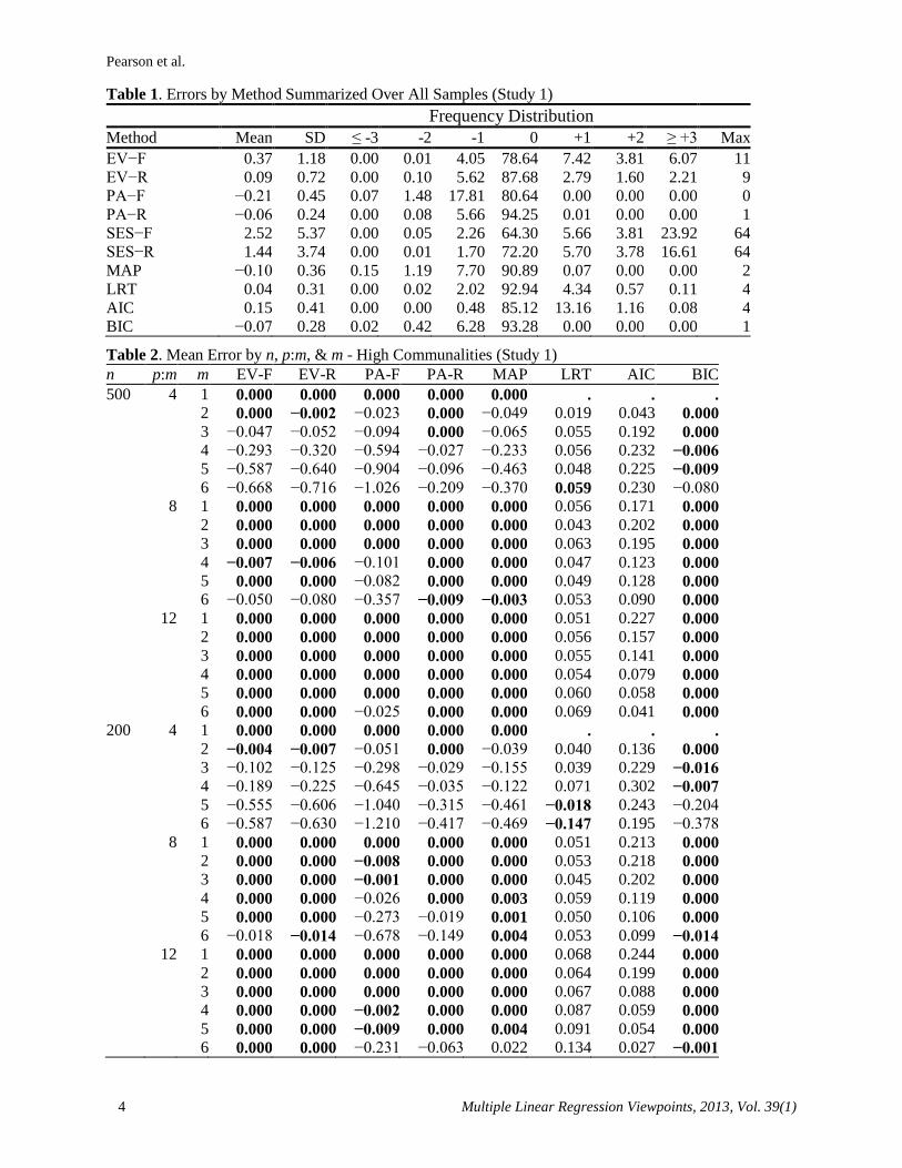
The primary outcome measure for the application of a procedure to a sample is the error of estimate,

. Table 1 presents a grand summary of d for the 10 decision methods over the 216,000

samples. These summary statistics can only be interpreted with respect to the 216 examined conditions

and are not estimates of any general characteristic of the procedures. In addition to the mean error, the

standard deviation is also provided, which is a measure of the observed consistency of each procedure.

Following the means and standard deviations are the percentages of samples that yielded specific values

of d. Finally, the maximum value is provided to show the presence of gross overestimates.

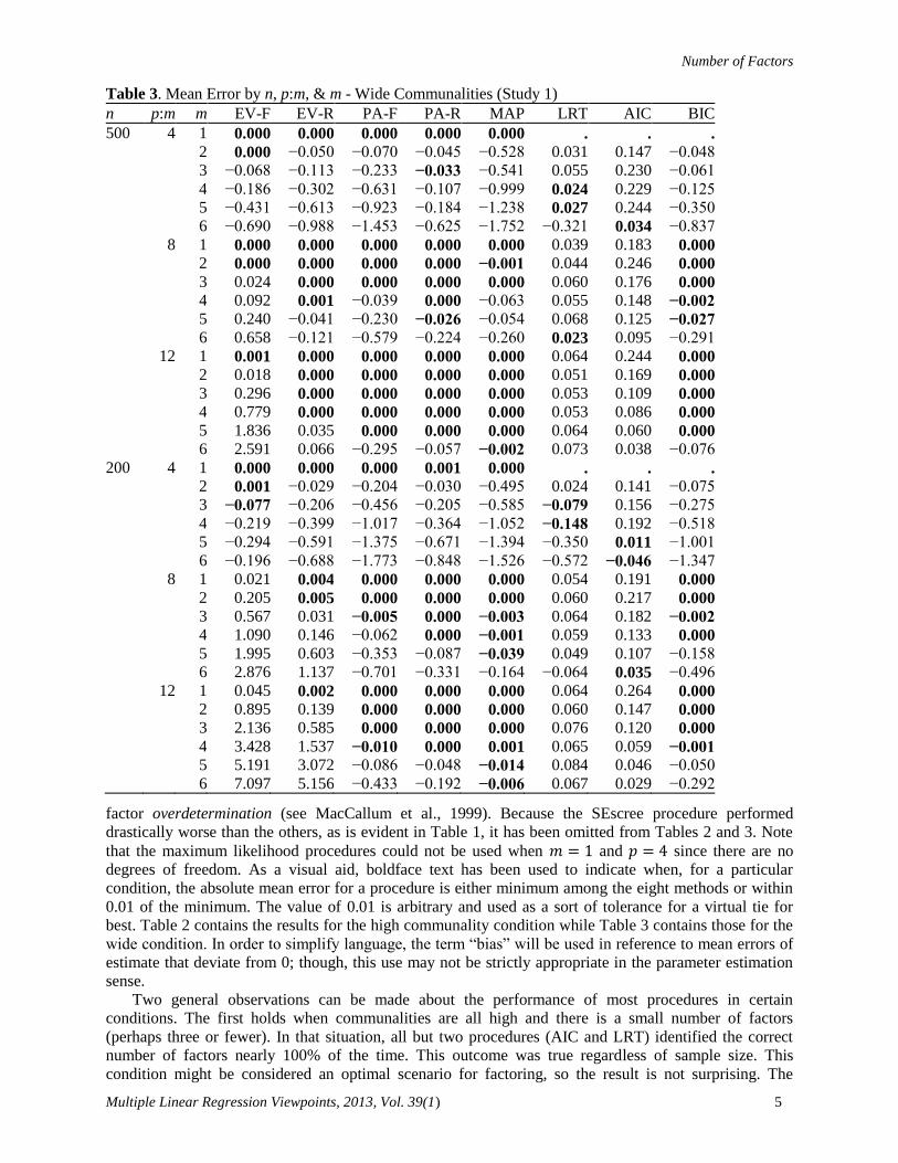
In Tables 2 and 3, the mean error for each procedure are presented for combinations of sample size,

variable-to-factor ratio, and number of factors. For the sake of space, only ratios of 4, 8, and 12 are

tabulated. These values can be viewed as respectively representing very low, moderate, and high levels of

Pearson et al.

4 Multiple Linear Regression Viewpoints, 2013, Vol. 39(1)

Table 1. Errors by Method Summarized Over All Samples (Study 1)

Frequency Distribution

Method Mean SD ≤ -3 -2 -1 0 +1 +2 ≥ +3 Max

EV−F 0.37 1.18 0.00 0.01 4.05 78.64 7.42 3.81 6.07 11

EV−R 0.09 0.72 0.00 0.10 5.62 87.68 2.79 1.60 2.21 9

PA−F −0.21 0.45 0.07 1.48 17.81 80.64 0.00 0.00 0.00 0

PA−R −0.06 0.24 0.00 0.08 5.66 94.25 0.01 0.00 0.00 1

SES−F 2.52 5.37 0.00 0.05 2.26 64.30 5.66 3.81 23.92 64

SES−R 1.44 3.74 0.00 0.01 1.70 72.20 5.70 3.78 16.61 64

MAP −0.10 0.36 0.15 1.19 7.70 90.89 0.07 0.00 0.00 2

LRT 0.04 0.31 0.00 0.02 2.02 92.94 4.34 0.57 0.11 4

AIC 0.15 0.41 0.00 0.00 0.48 85.12 13.16 1.16 0.08 4

BIC −0.07 0.28 0.02 0.42 6.28 93.28 0.00 0.00 0.00 1

Table 2. Mean Error by n, p:m, & m - High Communalities (Study 1)

n p:m m EV-F EV-R PA-F PA-R MAP LRT AIC BIC

500 4 1 0.000 0.000 0.000 0.000 0.000 . . . 2 0.000 −0.002 −0.023 0.000 −0.049 0.019 0.043 0.000 3 −0.047 −0.052 −0.094 0.000 −0.065 0.055 0.192 0.000 4 −0.293 −0.320 −0.594 −0.027 −0.233 0.056 0.232 −0.006 5 −0.587 −0.640 −0.904 −0.096 −0.463 0.048 0.225 −0.009 6 −0.668 −0.716 −1.026 −0.209 −0.370 0.059 0.230 −0.080

8 1 0.000 0.000 0.000 0.000 0.000 0.056 0.171 0.000 2 0.000 0.000 0.000 0.000 0.000 0.043 0.202 0.000 3 0.000 0.000 0.000 0.000 0.000 0.063 0.195 0.000 4 −0.007 −0.006 −0.101 0.000 0.000 0.047 0.123 0.000 5 0.000 0.000 −0.082 0.000 0.000 0.049 0.128 0.000 6 −0.050 −0.080 −0.357 −0.009 −0.003 0.053 0.090 0.000 12 1 0.000 0.000 0.000 0.000 0.000 0.051 0.227 0.000 2 0.000 0.000 0.000 0.000 0.000 0.056 0.157 0.000 3 0.000 0.000 0.000 0.000 0.000 0.055 0.141 0.000 4 0.000 0.000 0.000 0.000 0.000 0.054 0.079 0.000 5 0.000 0.000 0.000 0.000 0.000 0.060 0.058 0.000 6 0.000 0.000 −0.025 0.000 0.000 0.069 0.041 0.000 200 4 1 0.000 0.000 0.000 0.000 0.000 . . . 2 −0.004 −0.007 −0.051 0.000 −0.039 0.040 0.136 0.000 3 −0.102 −0.125 −0.298 −0.029 −0.155 0.039 0.229 −0.016 4 −0.189 −0.225 −0.645 −0.035 −0.122 0.071 0.302 −0.007 5 −0.555 −0.606 −1.040 −0.315 −0.461 −0.018 0.243 −0.204

6 −0.587 −0.630 −1.210 −0.417 −0.469 −0.147 0.195 −0.378

8 1 0.000 0.000 0.000 0.000 0.000 0.051 0.213 0.000 2 0.000 0.000 −0.008 0.000 0.000 0.053 0.218 0.000 3 0.000 0.000 −0.001 0.000 0.000 0.045 0.202 0.000 4 0.000 0.000 −0.026 0.000 0.003 0.059 0.119 0.000 5 0.000 0.000 −0.273 −0.019 0.001 0.050 0.106 0.000 6 −0.018 −0.014 −0.678 −0.149 0.004 0.053 0.099 −0.014 12 1 0.000 0.000 0.000 0.000 0.000 0.068 0.244 0.000 2 0.000 0.000 0.000 0.000 0.000 0.064 0.199 0.000 3 0.000 0.000 0.000 0.000 0.000 0.067 0.088 0.000 4 0.000 0.000 −0.002 0.000 0.000 0.087 0.059 0.000 5 0.000 0.000 −0.009 0.000 0.004 0.091 0.054 0.000 6 0.000 0.000 −0.231 −0.063 0.022 0.134 0.027 −0.001

Number of Factors

Multiple Linear Regression Viewpoints, 2013, Vol. 39(1) 5

Table 3. Mean Error by n, p:m, & m - Wide Communalities (Study 1)

n p:m m EV-F EV-R PA-F PA-R MAP LRT AIC BIC

500 4 1 0.000 0.000 0.000 0.000 0.000 . . . 2 0.000 −0.050 −0.070 −0.045 −0.528 0.031 0.147 −0.048

3 −0.068 −0.113 −0.233 −0.033 −0.541 0.055 0.230 −0.061

4 −0.186 −0.302 −0.631 −0.107 −0.999 0.024 0.229 −0.125

5 −0.431 −0.613 −0.923 −0.184 −1.238 0.027 0.244 −0.350

6 −0.690 −0.988 −1.453 −0.625 −1.752 −0.321 0.034 −0.837

8 1 0.000 0.000 0.000 0.000 0.000 0.039 0.183 0.000 2 0.000 0.000 0.000 0.000 −0.001 0.044 0.246 0.000 3 0.024 0.000 0.000 0.000 0.000 0.060 0.176 0.000 4 0.092 0.001 −0.039 0.000 −0.063 0.055 0.148 −0.002 5 0.240 −0.041 −0.230 −0.026 −0.054 0.068 0.125 −0.027 6 0.658 −0.121 −0.579 −0.224 −0.260 0.023 0.095 −0.291

12 1 0.001 0.000 0.000 0.000 0.000 0.064 0.244 0.000 2 0.018 0.000 0.000 0.000 0.000 0.051 0.169 0.000 3 0.296 0.000 0.000 0.000 0.000 0.053 0.109 0.000 4 0.779 0.000 0.000 0.000 0.000 0.053 0.086 0.000 5 1.836 0.035 0.000 0.000 0.000 0.064 0.060 0.000 6 2.591 0.066 −0.295 −0.057 −0.002 0.073 0.038 −0.076

200 4 1 0.000 0.000 0.000 0.001 0.000 . . . 2 0.001 −0.029 −0.204 −0.030 −0.495 0.024 0.141 −0.075

3 −0.077 −0.206 −0.456 −0.205 −0.585 −0.079 0.156 −0.275

4 −0.219 −0.399 −1.017 −0.364 −1.052 −0.148 0.192 −0.518

5 −0.294 −0.591 −1.375 −0.671 −1.394 −0.350 0.011 −1.001

6 −0.196 −0.688 −1.773 −0.848 −1.526 −0.572 −0.046 −1.347

8 1 0.021 0.004 0.000 0.000 0.000 0.054 0.191 0.000 2 0.205 0.005 0.000 0.000 0.000 0.060 0.217 0.000 3 0.567 0.031 −0.005 0.000 −0.003 0.064 0.182 −0.002 4 1.090 0.146 −0.062 0.000 −0.001 0.059 0.133 0.000 5 1.995 0.603 −0.353 −0.087 −0.039 0.049 0.107 −0.158

6 2.876 1.137 −0.701 −0.331 −0.164 −0.064 0.035 −0.496

12 1 0.045 0.002 0.000 0.000 0.000 0.064 0.264 0.000 2 0.895 0.139 0.000 0.000 0.000 0.060 0.147 0.000 3 2.136 0.585 0.000 0.000 0.000 0.076 0.120 0.000 4 3.428 1.537 −0.010 0.000 0.001 0.065 0.059 −0.001 5 5.191 3.072 −0.086 −0.048 −0.014 0.084 0.046 −0.050

6 7.097 5.156 −0.433 −0.192 −0.006 0.067 0.029 −0.292

factor overdetermination (see MacCallum et al., 1999). Because the SEscree procedure performed

drastically worse than the others, as is evident in Table 1, it has been omitted from Tables 2 and 3. Note

that the maximum likelihood procedures could not be used when and since there are no

degrees of freedom. As a visual aid, boldface text has been used to indicate when, for a particular

condition, the absolute mean error for a procedure is either minimum among the eight methods or within

0.01 of the minimum. The value of 0.01 is arbitrary and used as a sort of tolerance for a virtual tie for

best. Table 2 contains the results for the high communality condition while Table 3 contains those for the

wide condition. In order to simplify language, the term “bias” will be used in reference to mean errors of

estimate that deviate from 0; though, this use may not be strictly appropriate in the parameter estimation

sense.

Two general observations can be made about the performance of most procedures in certain

conditions. The first holds when communalities are all high and there is a small number of factors

(perhaps three or fewer). In that situation, all but two procedures (AIC and LRT) identified the correct

number of factors nearly 100% of the time. This outcome was true regardless of sample size. This

condition might be considered an optimal scenario for factoring, so the result is not surprising. The

Pearson et al.

6 Multiple Linear Regression Viewpoints, 2013, Vol. 39(1)

second general tendency is for most procedures to perform quite poorly when there are many factors and

few variables per factor. In this case, they frequently underestimated the number of factors. This finding

also is to be expected.

Eigenvalue Rules. The common factor eigenvalue rule was generally superior to Kaiser’s rule. The

former was both less biased and more consistent than the latter. In approximately 10% of samples, the

EV-F method overestimated m by two or more factors. In general, both procedures tended to overfactor

more as the number of variables increased.

When all communalities were high, the two eigenvalue rules performed very similarly. This result is

not surprising since RSMC is quite similar to R in that condition. In that case, they performed quite well in

terms of identifying the correct number of factors when there were three or fewer factors. When more

factors were present, these rules still performed very well when the ratio was high but increasingly

poorly as that ratio decreased to six or fewer variables per factor. As with most of the procedures,

underfactoring was quite pronounced when . When all communalities were high, the accuracy of

the eigenvalue rules was largely unaffected by sample size.

In the wide communality condition, the EV rules had dissimilar bias for most combinations of ,

m, and n. The common factor variant almost entirely outperformed Kaiser’s rule, with the exception that

EV-F underfactored less badly than EV-R when there were five or six factors and the ratio was very

small. For example, the respective bias for EV-F and EV-R were −0.69 versus −0.99 when ,

, and , and −0.20 versus −0.69 when . In all other situations, both EV rules were

quite likely to overfactor with EV-F doing so more often and by a greater margin. The miss rate for the

Kaiser’s rule increased consistently to nearly 100% as the ratio increased from about 7 to the

maximum of 12. At the smaller sample size of 200, the EV-R rule was also negatively affected by greater

ratios for models with at least three factors, but not to the extent of EV-F. When p is large, both

procedures were capable of gross overestimation. In the most extreme examined situation in which there

were 6 factors and , the mean error of estimate for EV-F was 7.10 and 2.59 for sample sizes of

200 and 500, respectively. Thus, the average number of factors suggested by Kaiser’s rule was 13 (for n =

200). In the same scenario, EV-R was nearly as bad when ( ) but among the best

methods when ( ) =0.07.

Parallel Analysis. Comparing the two PA approaches, the common factor version was as accurate or

better than the principal components version in all of the 216 conditions. For both PA-F and PA-R, the

type of error they were susceptible to was underfactoring. The PA-F procedure was the most negatively

biased procedure overall and consistently exhibited increasing likelihood of underfactoring as

decreased. Note that PA-F never overestimated m. Parallel analysis of the reduced correlation matrix was

perhaps the most consistently accurate of the 10 decision methods. In all, PA-R was correct 94.2% of the

time and wrong by −1 in 5.7% of samples. When , the error rate of PA-R was extremely low

except in cases from the wide communality condition with six factors and . At the smaller

sample size, PA-R still was quite accurate except for large models with very few variables per factor.

Even in the worst situation when , though it was negatively biased, it was less so than the other

procedures excluding LRT and AIC, which generally functioned “differently” from the rest. The PA-R

method was also the most consistent with .

SEscree and MAP. Overall, the standard error scree tests were the least accurate of the decision

methods. Although they performed well in some circumstances, in almost every condition in which p was

large (roughly ), both procedures were likely to dramatically overfactor. In the worst condition

( , wide communalities, , ), the average error for SES-R and SES-F were 22 and

30, respectively. For the entire study, these procedures overestimated m by three or more roughly 20% of

the time. In terms of the overall hit rate, the MAP procedure was fourth best at 90.9%. As with parallel

analysis, MAP only showed susceptibility to underfactoring and was prone to this error in the same

conditions as most of the other decision methods (several factors with low ratio). However, the

average magnitude of underestimation was substantially greater than procedures such as PA-R, BIC, and

EV-R. MAP was much more accurate in the high communality level than the wide level. Sample size did

not appear to have much of an impact on the success of the MAP method.

Number of Factors

Multiple Linear Regression Viewpoints, 2013, Vol. 39(1) 7

Maximum Likelihood Methods. The likelihood ratio test with Bartlett’s correction had the smallest

absolute mean error of estimate, was quite consistent ( ), and was correct in 93% of

attempts. Generally, the LRT appeared to be an extremely robust statistical test; as it produced incorrect

estimates (primarily ) approximately 5% of the time in nearly every condition. It deviated from

this nominal rate only when m was large and was small, particularly under the smaller sample size of

. Other than the under-determined conditions, LRT was fairly consistent across the two sample

sizes. The flip side of this consistency was that LRT maintained an error rate around 5% in cells where

nearly all of the other procedures were virtually flawless (high communalities and few factors). LRT was

within one factor of the correct value in over 99% of samples.

Both of the information criteria were accurate at estimating m, but BIC was the better of the two. The

AIC approach showed only slight positive bias and was fairly consistent ( ). Other than

the SEscree methods, AIC was most likely to overfactor (14%), even more than Kaiser’s rule. It was

exactly correct 85% of the time, compared to 93% for BIC. Across most conditions, the AIC method

overfactored by one in 10% to 20% of replications. As with LRT, this error rate was still observed in the

conditions that yielded nearly perfect performance by the other eight procedures.

Using the BIC was a very effective procedure for estimating the number of factors. Only PA-R had a

higher hit rate and, like PA-R, estimated either the correct number or one fewer in nearly every sample

(99.5% for BIC and 99.9% for PA-R). The BIC method was slightly more prone to underfactoring by two

than was PA-R. When communalities were wide, the BIC approach, like most other decision methods,

exhibited negative bias when the variable-to-factor ratio was very small.

Study Two

Methods

A second, independent simulation study was conducted, which, again, compared the performance of

the 10 decision methods. The primary motivation was to investigate the impact of correlation among

factors since this was a key limitation of Study 1. The existence of correlated factors is commonly

appreciated in the behavioral sciences (Fabrigar et al., 1999; Gorsuch, 1997; Preacher & MacCallum,

2003) and it was thought quite possible that the presence of such correlation could have a bearing on these

procedures. The imposition of interfactor correlations by way of:

R – U = LCL′ (1)

Where R – U is the model-implied reduced correlation matrix, L is a matrix of input factor loadings, and

C is a matrix of correlations among factors necessitated a different scheme for generating population

correlation matrices. A random L matrix generated by the Tucker-Koopman-Linn procedure is prone to

produce diagonal elements greater than unity after multiplication in equation 1. An additional concern

about the Tucker-Koopman-Linn system is that it frequently produces L matrices that may be somewhat

unrealistic in practice. An example of this is shown in Table 4 with loadings generated from the high

communality condition. It is common for manifest variables to load on multiple factors; however, it is

relatively rare in practice to observe for a variable multiple loadings that are greater than 0.5 or 0.6. This

occurrence is fairly common when using this algorithm (under the orthogonal model).

With the above considerations in mind, a different data generation scheme was used in Study 2.

Loading matrices were created to have perfect simple structure. For example, if ratio was 6, the first

6 variables loaded on factor 1, the next 6 on factor 2, and so forth. All non-major loadings were set to

zero. Again, it was desired to randomly generate each loading in order to increase the generalizability of

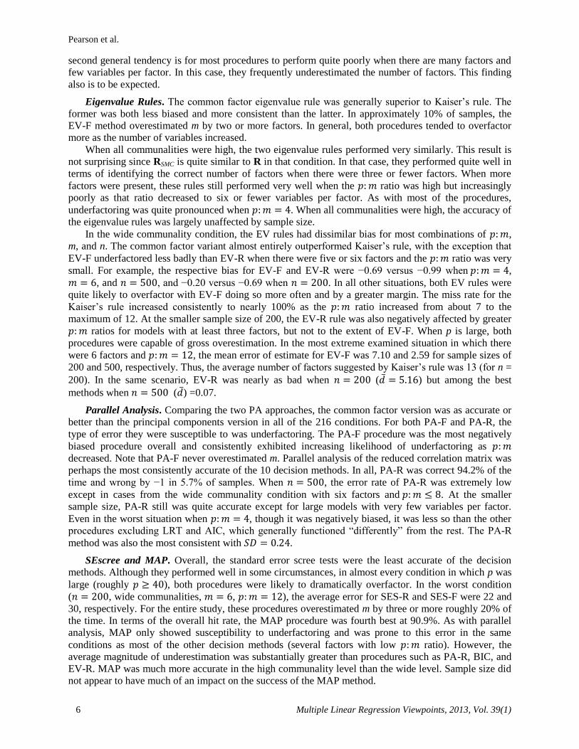
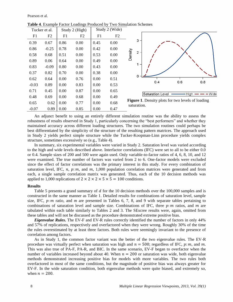
results. In this study, non-zero factor loadings were generated from the beta distribution on the interval

(0.3, 0.9). Two different sets of parameters were used to achieve two levels of saturation termed “high”

and “wide” to mimic the communality levels of Study 1. The specific parameter values were selected by

trial-and-error. For the high saturation level, and for the wide level, .

Figure 1 shows the probability density of each distribution. Examples of loadings generated by this

scheme for the high and wide saturation levels can be seen in Table 4. Once the input factor loadings were

determined, the population correlation matrix R was created via equation 1and then placing ones on the

diagonal. Finally, the Wijsman method (described by Hong, 1999) was then employed to generate a

random sample correlation matrix directly from R without creating an observation-level data matrix.

Pearson et al.

8 Multiple Linear Regression Viewpoints, 2013, Vol. 39(1)

Table 4. Example Factor Loadings Produced by Two Simulation Schemes

Tucker et al. Study 2 (High) Study 2 (Wide)

F1 F2 F1 F2 F1 F2

0.39 0.67 0.86 0.00 0.45 0.00

0.86 -0.25 0.78 0.00 0.42 0.00

0.58 0.68 0.51 0.00 0.53 0.00

0.89 0.06 0.64 0.00 0.49 0.00

0.83 -0.09 0.80 0.00 0.43 0.00

0.37 0.82 0.70 0.00 0.38 0.00

0.62 0.64 0.00 0.76 0.00 0.51

-0.03 0.89 0.00 0.83 0.00 0.53

0.71 0.45 0.00 0.87 0.00 0.65

0.48 0.69 0.00 0.68 0.00 0.49

0.65 0.62 0.00 0.77 0.00 0.68

-0.07 0.89 0.00 0.85 0.00 0.47

An adjunct benefit to using an entirely different simulation routine was the ability to assess the

robustness of results observed in Study 1, particularly concerning the “best performers” and whether they

maintained accuracy across different loading structures. The two simulation routines could perhaps be

best differentiated by the simplicity of the structure of the resulting pattern matrices. The approach used

in Study 2 yields perfect simple structure while the Tucker-Koopman-Linn procedure yields complex

structure, sometimes excessively so (e.g., Table 4).

In summary, six experimental variables were varied in Study 2. Saturation level was varied according

to the high and wide levels described above. Interfactor correlations (IFC) were set to all to be either 0.0

or 0.4. Sample sizes of 200 and 500 were again used. Only variable-to-factor ratios of 4, 6, 8, 10, and 12

were examined. The true number of factors was varied from 2 to 6. One-factor models were excluded

since the effect of factor correlations was the primary interest in this study. For every combination of

saturation level, IFC, , , and , 1,000 population correlation matrices were generated and from

each, a single sample correlation matrix was generated. Thus, each of the 10 decision methods was

applied to 1,000 replications of conditions.

Results

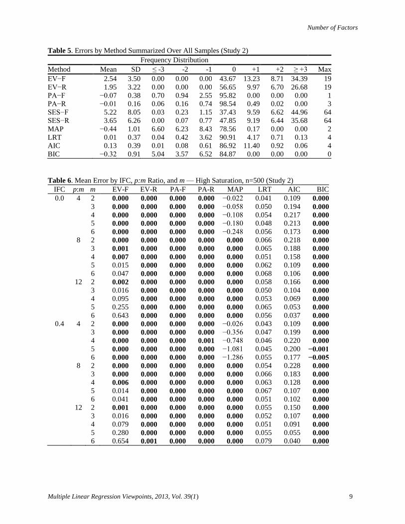
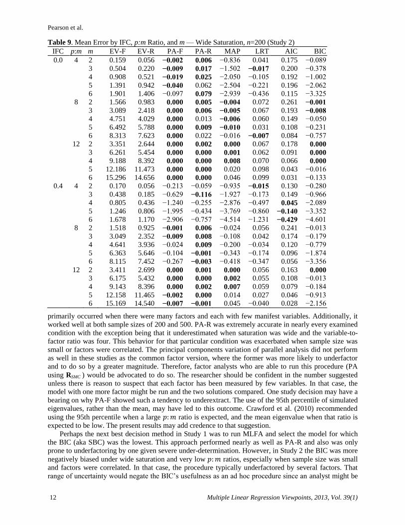
Table 5 presents a grand summary of for the 10 decision methods over the 100,000 samples and is

constructed in the same manner as Table 1. Detailed results for combinations of saturation level, sample

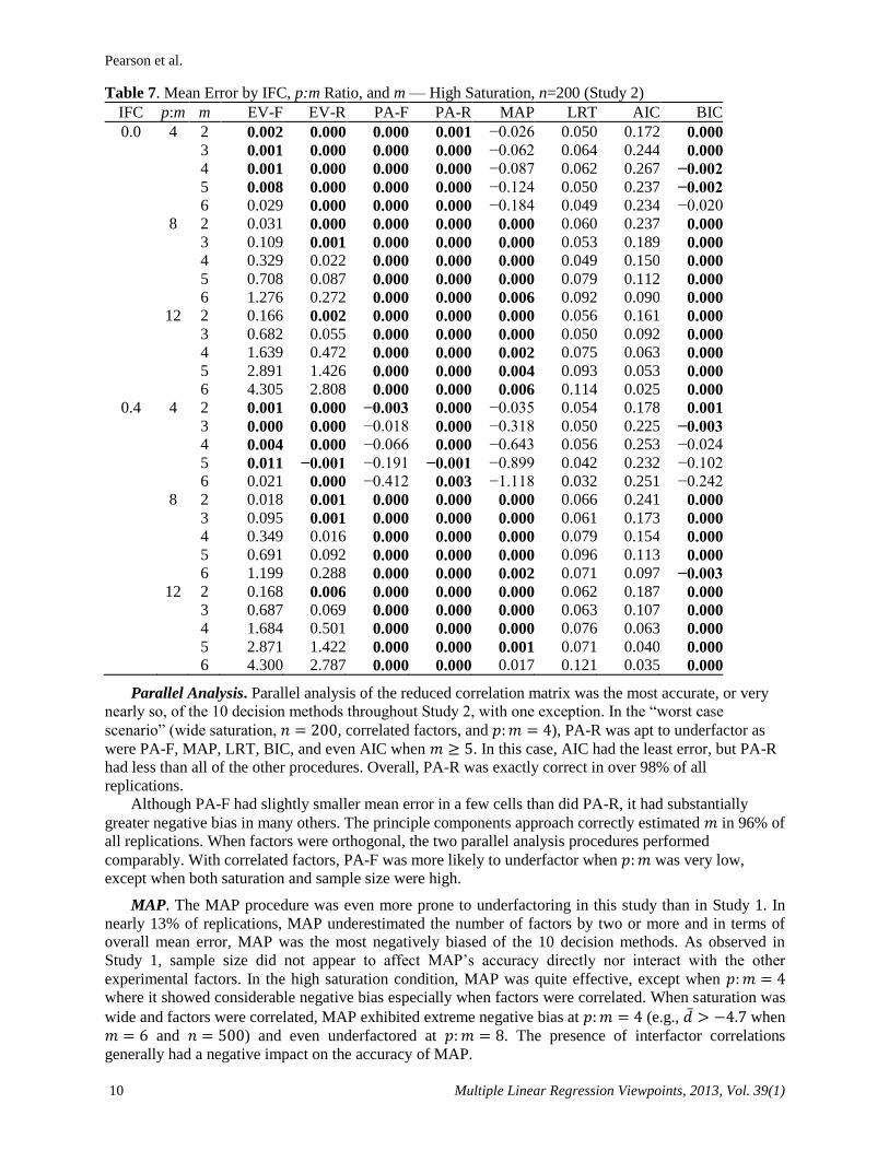
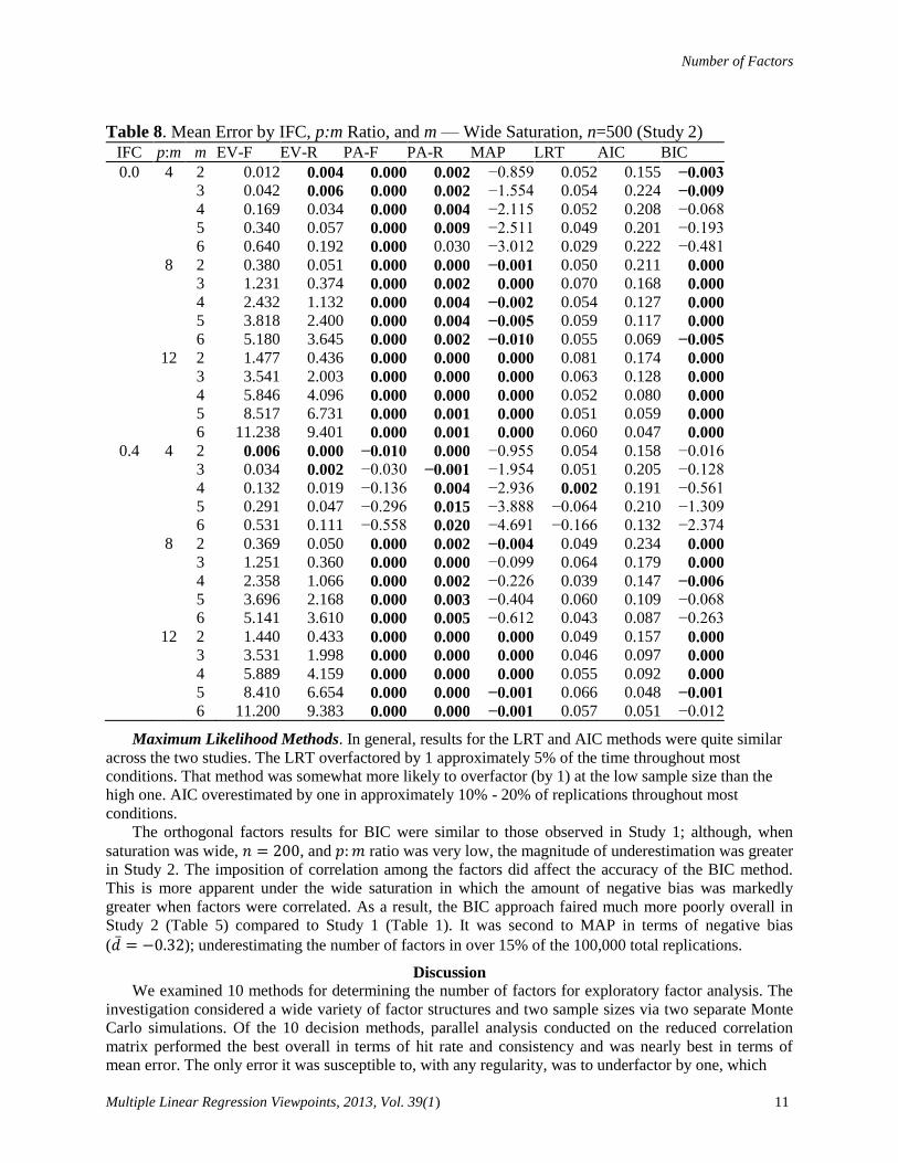
size, IFC, ratio, and m are presented in Tables 6, 7, 8, and 9 with separate tables pertaining to

combinations of saturation level and sample size. Combinations of IFC, three ratios, and are

tabulated within each table similarly to Tables 2 and 3. The SEscree results were, again, omitted from

these tables and will not be discussed as the procedure demonstrated extreme positive bias.

Eigenvalue Rules. The EV-F and EV-R rules correctly identified the number of factors in only 44%

and 57% of replications, respectively and overfactored when they were wrong. Roughly 30% of the time

the rules overestimated by at least three factors. Both rules were seemingly invariant to the presence of

correlation among factors.

As in Study 1, the common factor variant was the better of the two eigenvalue rules. The EV-R

procedure was virtually perfect when saturation was high and ; regardless of IFC, , and .

This was also true of PA-F, PA-R, and BIC. In the same scenario, EV-F began to overfactor when the

number of variables increased beyond about 40. When or saturation was wide, both eigenvalue

methods demonstrated increasing positive bias for models with more variables. The two rules both

overfactored in most of the same conditions, but the magnitude of positive bias was always greater for

EV-F. In the wide saturation condition, both eigenvalue methods were quite biased, and extremely so,

when .

Figure 1. Density plots for two levels of loading

saturation.

Number of Factors

Multiple Linear Regression Viewpoints, 2013, Vol. 39(1) 9

Table 5. Errors by Method Summarized Over All Samples (Study 2)

Frequency Distribution

Method Mean SD ≤ -3 -2 -1 0 +1 +2 ≥ +3 Max

EV−F 2.54 3.50 0.00 0.00 0.00 43.67 13.23 8.71 34.39 19

EV−R 1.95 3.22 0.00 0.00 0.00 56.65 9.97 6.70 26.68 19

PA−F −0.07 0.38 0.70 0.94 2.55 95.82 0.00 0.00 0.00 1

PA−R −0.01 0.16 0.06 0.16 0.74 98.54 0.49 0.02 0.00 3

SES−F 5.22 8.05 0.03 0.23 1.15 37.43 9.59 6.62 44.96 64

SES−R 3.65 6.26 0.00 0.07 0.77 47.85 9.19 6.44 35.68 64

MAP −0.44 1.01 6.60 6.23 8.43 78.56 0.17 0.00 0.00 2

LRT 0.01 0.37 0.04 0.42 3.62 90.91 4.17 0.71 0.13 4

AIC 0.13 0.39 0.01 0.08 0.61 86.92 11.40 0.92 0.06 4

BIC −0.32 0.91 5.04 3.57 6.52 84.87 0.00 0.00 0.00 0

Table 6. Mean Error by IFC, p:m Ratio, and m — High Saturation, n=500 (Study 2)

IFC p:m m EV-F EV-R PA-F PA-R MAP LRT AIC BIC

0.0 4 2 0.000 0.000 0.000 0.000 −0.022 0.041 0.109 0.000 3 0.000 0.000 0.000 0.000 −0.058 0.050 0.194 0.000 4 0.000 0.000 0.000 0.000 −0.108 0.054 0.217 0.000 5 0.000 0.000 0.000 0.000 −0.180 0.048 0.213 0.000 6 0.000 0.000 0.000 0.000 −0.248 0.056 0.173 0.000 8 2 0.000 0.000 0.000 0.000 0.000 0.066 0.218 0.000 3 0.001 0.000 0.000 0.000 0.000 0.065 0.188 0.000 4 0.007 0.000 0.000 0.000 0.000 0.051 0.158 0.000 5 0.015 0.000 0.000 0.000 0.000 0.062 0.109 0.000 6 0.047 0.000 0.000 0.000 0.000 0.068 0.106 0.000 12 2 0.002 0.000 0.000 0.000 0.000 0.058 0.166 0.000 3 0.016 0.000 0.000 0.000 0.000 0.050 0.104 0.000 4 0.095 0.000 0.000 0.000 0.000 0.053 0.069 0.000 5 0.255 0.000 0.000 0.000 0.000 0.065 0.053 0.000 6 0.643 0.000 0.000 0.000 0.000 0.056 0.037 0.000

0.4 4 2 0.000 0.000 0.000 0.000 −0.026 0.043 0.109 0.000 3 0.000 0.000 0.000 0.000 −0.356 0.047 0.199 0.000 4 0.000 0.000 0.000 0.001 −0.748 0.046 0.220 0.000 5 0.000 0.000 0.000 0.000 −1.081 0.045 0.200 −0.001 6 0.000 0.000 0.000 0.000 −1.286 0.055 0.177 −0.005 8 2 0.000 0.000 0.000 0.000 0.000 0.054 0.228 0.000 3 0.000 0.000 0.000 0.000 0.000 0.066 0.183 0.000 4 0.006 0.000 0.000 0.000 0.000 0.063 0.128 0.000 5 0.014 0.000 0.000 0.000 0.000 0.067 0.107 0.000 6 0.041 0.000 0.000 0.000 0.000 0.051 0.102 0.000 12 2 0.001 0.000 0.000 0.000 0.000 0.055 0.150 0.000 3 0.016 0.000 0.000 0.000 0.000 0.052 0.107 0.000 4 0.079 0.000 0.000 0.000 0.000 0.051 0.091 0.000 5 0.280 0.000 0.000 0.000 0.000 0.055 0.055 0.000 6 0.654 0.001 0.000 0.000 0.000 0.079 0.040 0.000

Pearson et al.

10 Multiple Linear Regression Viewpoints, 2013, Vol. 39(1)

Table 7. Mean Error by IFC, p:m Ratio, and m — High Saturation, n=200 (Study 2)

IFC p:m m EV-F EV-R PA-F PA-R MAP LRT AIC BIC

0.0 4 2 0.002 0.000 0.000 0.001 −0.026 0.050 0.172 0.000 3 0.001 0.000 0.000 0.000 −0.062 0.064 0.244 0.000 4 0.001 0.000 0.000 0.000 −0.087 0.062 0.267 −0.002 5 0.008 0.000 0.000 0.000 −0.124 0.050 0.237 −0.002 6 0.029 0.000 0.000 0.000 −0.184 0.049 0.234 −0.020

8 2 0.031 0.000 0.000 0.000 0.000 0.060 0.237 0.000 3 0.109 0.001 0.000 0.000 0.000 0.053 0.189 0.000 4 0.329 0.022 0.000 0.000 0.000 0.049 0.150 0.000 5 0.708 0.087 0.000 0.000 0.000 0.079 0.112 0.000 6 1.276 0.272 0.000 0.000 0.006 0.092 0.090 0.000 12 2 0.166 0.002 0.000 0.000 0.000 0.056 0.161 0.000 3 0.682 0.055 0.000 0.000 0.000 0.050 0.092 0.000 4 1.639 0.472 0.000 0.000 0.002 0.075 0.063 0.000 5 2.891 1.426 0.000 0.000 0.004 0.093 0.053 0.000 6 4.305 2.808 0.000 0.000 0.006 0.114 0.025 0.000

0.4 4 2 0.001 0.000 −0.003 0.000 −0.035 0.054 0.178 0.001 3 0.000 0.000 −0.018 0.000 −0.318 0.050 0.225 −0.003 4 0.004 0.000 −0.066 0.000 −0.643 0.056 0.253 −0.024

5 0.011 −0.001 −0.191 −0.001 −0.899 0.042 0.232 −0.102

6 0.021 0.000 −0.412 0.003 −1.118 0.032 0.251 −0.242

8 2 0.018 0.001 0.000 0.000 0.000 0.066 0.241 0.000 3 0.095 0.001 0.000 0.000 0.000 0.061 0.173 0.000 4 0.349 0.016 0.000 0.000 0.000 0.079 0.154 0.000 5 0.691 0.092 0.000 0.000 0.000 0.096 0.113 0.000 6 1.199 0.288 0.000 0.000 0.002 0.071 0.097 −0.003 12 2 0.168 0.006 0.000 0.000 0.000 0.062 0.187 0.000 3 0.687 0.069 0.000 0.000 0.000 0.063 0.107 0.000 4 1.684 0.501 0.000 0.000 0.000 0.076 0.063 0.000 5 2.871 1.422 0.000 0.000 0.001 0.071 0.040 0.000 6 4.300 2.787 0.000 0.000 0.017 0.121 0.035 0.000

Parallel Analysis. Parallel analysis of the reduced correlation matrix was the most accurate, or very

nearly so, of the 10 decision methods throughout Study 2, with one exception. In the “worst case

scenario” (wide saturation, , correlated factors, and ), PA-R was apt to underfactor as

were PA-F, MAP, LRT, BIC, and even AIC when . In this case, AIC had the least error, but PA-R

had less than all of the other procedures. Overall, PA-R was exactly correct in over 98% of all

replications.

Although PA-F had slightly smaller mean error in a few cells than did PA-R, it had substantially

greater negative bias in many others. The principle components approach correctly estimated in 96% of

all replications. When factors were orthogonal, the two parallel analysis procedures performed

comparably. With correlated factors, PA-F was more likely to underfactor when was very low,

except when both saturation and sample size were high.

MAP. The MAP procedure was even more prone to underfactoring in this study than in Study 1. In

nearly 13% of replications, MAP underestimated the number of factors by two or more and in terms of

overall mean error, MAP was the most negatively biased of the 10 decision methods. As observed in

Study 1, sample size did not appear to affect MAP’s accuracy directly nor interact with the other

experimental factors. In the high saturation condition, MAP was quite effective, except when

where it showed considerable negative bias especially when factors were correlated. When saturation was

wide and factors were correlated, MAP exhibited extreme negative bias at (e.g., when

and ) and even underfactored at . The presence of interfactor correlations

generally had a negative impact on the accuracy of MAP.

Number of Factors

Multiple Linear Regression Viewpoints, 2013, Vol. 39(1) 11

Table 8. Mean Error by IFC, p:m Ratio, and m — Wide Saturation, n=500 (Study 2)

IFC p:m m EV-F EV-R PA-F PA-R MAP LRT AIC BIC

0.0 4 2 0.012 0.004 0.000 0.002 −0.859 0.052 0.155 −0.003 3 0.042 0.006 0.000 0.002 −1.554 0.054 0.224 −0.009 4 0.169 0.034 0.000 0.004 −2.115 0.052 0.208 −0.068

5 0.340 0.057 0.000 0.009 −2.511 0.049 0.201 −0.193

6 0.640 0.192 0.000 0.030 −3.012 0.029 0.222 −0.481

8 2 0.380 0.051 0.000 0.000 −0.001 0.050 0.211 0.000 3 1.231 0.374 0.000 0.002 0.000 0.070 0.168 0.000 4 2.432 1.132 0.000 0.004 −0.002 0.054 0.127 0.000 5 3.818 2.400 0.000 0.004 −0.005 0.059 0.117 0.000 6 5.180 3.645 0.000 0.002 −0.010 0.055 0.069 −0.005 12 2 1.477 0.436 0.000 0.000 0.000 0.081 0.174 0.000 3 3.541 2.003 0.000 0.000 0.000 0.063 0.128 0.000 4 5.846 4.096 0.000 0.000 0.000 0.052 0.080 0.000 5 8.517 6.731 0.000 0.001 0.000 0.051 0.059 0.000 6 11.238 9.401 0.000 0.001 0.000 0.060 0.047 0.000

0.4 4 2 0.006 0.000 −0.010 0.000 −0.955 0.054 0.158 −0.016

3 0.034 0.002 −0.030 −0.001 −1.954 0.051 0.205 −0.128

4 0.132 0.019 −0.136 0.004 −2.936 0.002 0.191 −0.561

5 0.291 0.047 −0.296 0.015 −3.888 −0.064 0.210 −1.309

6 0.531 0.111 −0.558 0.020 −4.691 −0.166 0.132 −2.374

8 2 0.369 0.050 0.000 0.002 −0.004 0.049 0.234 0.000 3 1.251 0.360 0.000 0.000 −0.099 0.064 0.179 0.000 4 2.358 1.066 0.000 0.002 −0.226 0.039 0.147 −0.006 5 3.696 2.168 0.000 0.003 −0.404 0.060 0.109 −0.068

6 5.141 3.610 0.000 0.005 −0.612 0.043 0.087 −0.263

12 2 1.440 0.433 0.000 0.000 0.000 0.049 0.157 0.000 3 3.531 1.998 0.000 0.000 0.000 0.046 0.097 0.000 4 5.889 4.159 0.000 0.000 0.000 0.055 0.092 0.000 5 8.410 6.654 0.000 0.000 −0.001 0.066 0.048 −0.001 6 11.200 9.383 0.000 0.000 −0.001 0.057 0.051 −0.012

Maximum Likelihood Methods. In general, results for the LRT and AIC methods were quite similar

across the two studies. The LRT overfactored by 1 approximately 5% of the time throughout most

conditions. That method was somewhat more likely to overfactor (by 1) at the low sample size than the

high one. AIC overestimated by one in approximately 10% - 20% of replications throughout most

conditions.

The orthogonal factors results for BIC were similar to those observed in Study 1; although, when

saturation was wide, , and ratio was very low, the magnitude of underestimation was greater

in Study 2. The imposition of correlation among the factors did affect the accuracy of the BIC method.

This is more apparent under the wide saturation in which the amount of negative bias was markedly

greater when factors were correlated. As a result, the BIC approach faired much more poorly overall in

Study 2 (Table 5) compared to Study 1 (Table 1). It was second to MAP in terms of negative bias

( ); underestimating the number of factors in over 15% of the 100,000 total replications.

Discussion

We examined 10 methods for determining the number of factors for exploratory factor analysis. The

investigation considered a wide variety of factor structures and two sample sizes via two separate Monte

Carlo simulations. Of the 10 decision methods, parallel analysis conducted on the reduced correlation

matrix performed the best overall in terms of hit rate and consistency and was nearly best in terms of

mean error. The only error it was susceptible to, with any regularity, was to underfactor by one, which

Pearson et al.

12 Multiple Linear Regression Viewpoints, 2013, Vol. 39(1)

Table 9. Mean Error by IFC, p:m Ratio, and m — Wide Saturation, n=200 (Study 2)

IFC p:m m EV-F EV-R PA-F PA-R MAP LRT AIC BIC

0.0 4 2 0.159 0.056 −0.002 0.006 −0.836 0.041 0.175 −0.089

3 0.504 0.220 −0.009 0.017 −1.502 −0.017 0.200 −0.378

4 0.908 0.521 −0.019 0.025 −2.050 −0.105 0.192 −1.002

5 1.391 0.942 −0.040 0.062 −2.504 −0.221 0.196 −2.062

6 1.901 1.406 −0.097 0.079 −2.939 −0.436 0.115 −3.325

8 2 1.566 0.983 0.000 0.005 −0.004 0.072 0.261 −0.001 3 3.089 2.418 0.000 0.006 −0.005 0.067 0.193 −0.008 4 4.751 4.029 0.000 0.013 −0.006 0.060 0.149 −0.050

5 6.492 5.788 0.000 0.009 −0.010 0.031 0.108 −0.231

6 8.313 7.623 0.000 0.022 −0.016 −0.007 0.084 −0.757

12 2 3.351 2.644 0.000 0.002 0.000 0.067 0.178 0.000 3 6.261 5.454 0.000 0.000 0.001 0.062 0.091 0.000 4 9.188 8.392 0.000 0.000 0.008 0.070 0.066 0.000 5 12.186 11.473 0.000 0.000 0.020 0.098 0.043 −0.016

6 15.296 14.656 0.000 0.000 0.046 0.099 0.031 −0.133

0.4 4 2 0.170 0.056 −0.213 −0.059 −0.935 −0.015 0.130 −0.280

3 0.438 0.185 −0.629 −0.116 −1.927 −0.173 0.149 −0.966

4 0.805 0.436 −1.240 −0.255 −2.876 −0.497 0.045 −2.089

5 1.246 0.806 −1.995 −0.434 −3.769 −0.860 −0.140 −3.352

6 1.678 1.170 −2.906 −0.757 −4.514 −1.231 −0.429 −4.601

8 2 1.518 0.925 −0.001 0.006 −0.024 0.056 0.241 −0.013

3 3.049 2.352 −0.009 0.008 −0.108 0.042 0.174 −0.179

4 4.641 3.936 −0.024 0.009 −0.200 −0.034 0.120 −0.779

5 6.363 5.646 −0.104 −0.001 −0.343 −0.174 0.096 −1.874

6 8.115 7.452 −0.267 −0.003 −0.418 −0.347 0.056 −3.356

12 2 3.411 2.699 0.000 0.001 0.000 0.056 0.163 0.000 3 6.175 5.432 0.000 0.000 0.002 0.055 0.108 −0.013

4 9.143 8.396 0.000 0.002 0.007 0.059 0.079 −0.184

5 12.158 11.465 −0.002 0.000 0.014 0.027 0.046 −0.913

6 15.169 14.540 −0.007 −0.001 0.045 −0.040 0.028 −2.156

primarily occurred when there were many factors and each with few manifest variables. Additionally, it

worked well at both sample sizes of 200 and 500. PA-R was extremely accurate in nearly every examined

condition with the exception being that it underestimated when saturation was wide and the variable-to-

factor ratio was four. This behavior for that particular condition was exacerbated when sample size was

small or factors were correlated. The principal components variation of parallel analysis did not perform

as well in these studies as the common factor version, where the former was more likely to underfactor

and to do so by a greater magnitude. Therefore, factor analysts who are able to run this procedure (PA

using RSMC ) would be advocated to do so. The researcher should be confident in the number suggested

unless there is reason to suspect that each factor has been measured by few variables. In that case, the

model with one more factor might be run and the two solutions compared. One study decision may have a

bearing on why PA-F showed such a tendency to underextract. The use of the 95th percentile of simulated

eigenvalues, rather than the mean, may have led to this outcome. Crawford et al. (2010) recommended

using the 95th percentile when a large ratio is expected, and the mean eigenvalue when that ratio is

expected to be low. The present results may add credence to that suggestion.

Perhaps the next best decision method in Study 1 was to run MLFA and select the model for which

the BIC (aka SBC) was the lowest. This approach performed nearly as well as PA-R and also was only

prone to underfactoring by one given severe under-determination. However, in Study 2 the BIC was more

negatively biased under wide saturation and very low ratios, especially when sample size was small

and factors were correlated. In that case, the procedure typically underfactored by several factors. That

range of uncertainty would negate the BIC’s usefulness as an ad hoc procedure since an analyst might be

Number of Factors

Multiple Linear Regression Viewpoints, 2013, Vol. 39(1) 13

forced to consider many candidate models. The other information criteria, the AIC, was consistently

likely to suggest one too many factors, but very rarely erred in another manner. Thus, for analysts who are

unable to run parallel analysis, but can obtain the AIC and BIC from common statistical software

packages, the following approach might be utilized. Run MLFA on several candidate models (e.g., 2 to 4

factors) and examine the information criteria. The model that has the lowest AIC should be examined as

should the next smaller model. The BIC might also be inspected in a similar manner, but should be used

warily unless final communality estimates all appear to be fairly high.

The likelihood ratio test was nearly as likely to be correct as PA-R or BIC, but had a small, notable

chance of suggesting the wrong number of factors in situations that posed no problems for other

procedures. Furthermore, the LRT was capable of both underfactoring in under-saturated conditions and

overfactoring by one or two (and up to four in rare cases). Thus, a researcher using the LRT to determine

the number of factors might need to consider comparing as many as five candidate models. If software

outputs the LRT along with the AIC, then the AIC should be utilized in the manner suggested above. If

only the LRT is given (as is the case in SPSS), it can still be used with confidence in many situations.

The ubiquitous eigenvalue-greater-than-one rule suggested by Kaiser was not shown to be

particularly accurate. This study replicated the well-known tendency of Kaiser’s rule to overfactor

(Browne, 1968; Gorsuch, 1983, 1997; Zwick & Velicer, 1986). It had the lowest overall hit rate outside of

the SEscree procedures and frequently yielded overestimates of two or more. In Study 1 when all

communalities were high (at least .6), this rule did work fairly well. When communalities had a greater

range (from .2 to .8), it worked quite poorly. When communalities were wide and there are many

variables relative to the number of factors, Kaiser’s rule suggested an average of 2 to 7 factors too many.

In Study 2, Kaiser’s rule overfactored even in the high saturation condition and did so by extreme

amounts when saturation was wide. It is the first author’s experience that a wide range of communalities,

or rotated factor loadings, are common in practice. Given that EV-F is the default method in major

software packages and has been shown in literature reviews to be common practice (Fabrigar et al., 1999;

Ford et al., 1986; Henson & Roberts, 2006; Park et al., 2002), it seems likely that researchers often

interpret more factors than are truly present in their data; perhaps many more.

Rather than retaining the number of factors with eigenvalues greater than one, researchers would be

somewhat better served using the conceptually similar criterion of the number of eigenvalues of the

reduced correlation matrix greater than the mean eigenvalue. If all communalities are high and the sample

size is large, then the common factor eigenvalue rule is likely to be correct. Otherwise, this method should

also be used with caution.

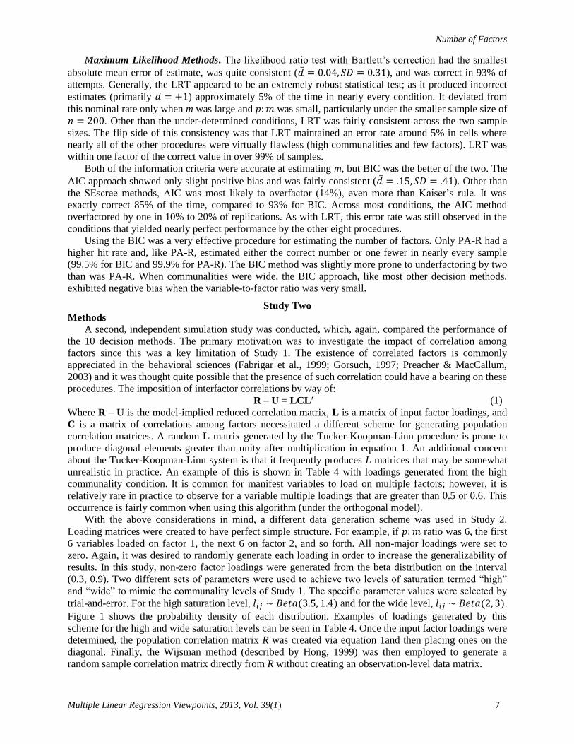
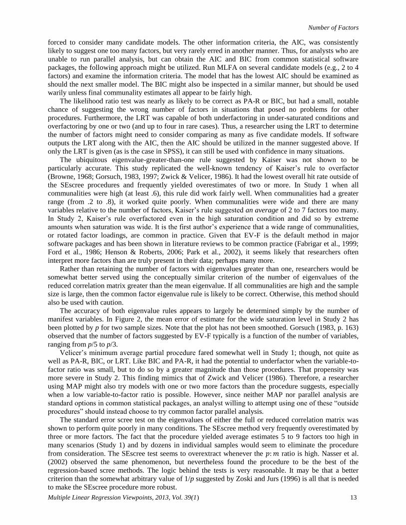
The accuracy of both eigenvalue rules appears to largely be determined simply by the number of

manifest variables. In Figure 2, the mean error of estimate for the wide saturation level in Study 2 has

been plotted by p for two sample sizes. Note that the plot has not been smoothed. Gorsuch (1983, p. 163)

observed that the number of factors suggested by EV-F typically is a function of the number of variables,

ranging from p/5 to p/3.

Velicer’s minimum average partial procedure fared somewhat well in Study 1; though, not quite as

well as PA-R, BIC, or LRT. Like BIC and PA-R, it had the potential to underfactor when the variable-to-

factor ratio was small, but to do so by a greater magnitude than those procedures. That propensity was

more severe in Study 2. This finding mimics that of Zwick and Velicer (1986). Therefore, a researcher

using MAP might also try models with one or two more factors than the procedure suggests, especially

when a low variable-to-factor ratio is possible. However, since neither MAP nor parallel analysis are

standard options in common statistical packages, an analyst willing to attempt using one of these “outside

procedures” should instead choose to try common factor parallel analysis.

The standard error scree test on the eigenvalues of either the full or reduced correlation matrix was

shown to perform quite poorly in many conditions. The SEscree method very frequently overestimated by

three or more factors. The fact that the procedure yielded average estimates 5 to 9 factors too high in

many scenarios (Study 1) and by dozens in individual samples would seem to eliminate the procedure

from consideration. The SEscree test seems to overextract whenever the ratio is high. Nasser et al.

(2002) observed the same phenomenon, but nevertheless found the procedure to be the best of the

regression-based scree methods. The logic behind the tests is very reasonable. It may be that a better

criterion than the somewhat arbitrary value of 1/p suggested by Zoski and Jurs (1996) is all that is needed

to make the SEscree procedure more robust.

Pearson et al.

14 Multiple Linear Regression Viewpoints, 2013, Vol. 39(1)

Figure 2. Mean error versus number of variables for

eight methods - wide saturation (Study 2).

One important limitation to this study is that

only sample sizes of 200 and 500 were used.

Several of the procedures may have been

adversely affected by more extreme values. In

particular, the LRT has been observed to

overfactor when n is very large, and 500 may

not have been enough to clearly see that

behavior.

Conclusions

Factor analysts needing to estimate the

number of common factors should give strong

consideration to using parallel analysis on the

reduced correlation matrix. A SAS macro to run

PA-R (as well as PA-F) can be requested from

the first author. When using this method, if it is

suspected that each factor is only represented by

a small number of variables (perhaps five or

fewer), then the researcher might also examine

the model with one more factor. Use of AIC to

determine the best model is also recommended with the caveat that the model with one fewer factor must

also be examined. If neither of these options is available, the number of observed variables is not too

large, and estimated communalities are all large, the analyst might use the number of eigenvalues in the

reduced correlation matrix greater than the mean; a decision method that was more accurate in this study

than was the traditional eigenvalues-over-one rule.

References

Akaike, H. (1973). Information theory and an extension of the maximum likelihood principle. In B. N.

Petrov & F. Csaki (Eds.), 2nd International Symposium on Information Theory (pp. 267-281).

Budapest: Akademiai Kiado.

Akaike, H. (1987). Factor analysis and AIC. Psychometrika, 52(3), 317-332.

Bartlett, M. S. (1950). Tests of significance in factor analysis. British Journal of Psychology, 3(3), 77-85.

Bartlett, M. S. (1951). A further note on tests of significance in factor analysis. British Journal of

Psychology, 4(4), 1-2.

Browne, M. W. (1968). A comparison of factor analytic techniques. Psychometrika, 33(3), 267-334.

Cattell, R. (1966). The scree test for the number of factors. Multivariate Behavioral Research, 1(2), 245-

276.

Cattell, R., & Vogelmann, S. (1977). A comprehensive trial of the scree and KG criteria for determining

the number of factors. Multivariate Behavioral Research, 12(3), 289-325.

Chen, R. (2003). An SAS/IML procedure for maximum likelihood factor analysis. Behavior Research

Methods, 35(2), 310–317.

Cota, A. A., Longman, R. S., Holden, R. R., & Fekken, G. C. (1993). Comparing different methods for

implementing parallel analysis: a practical index of accuracy. Educational and Psychological

Measurement, 53(4), 865 -876.

Crawford, A. V., Green, S. B., Levy, R., Lo, W. J., Scott, L., Svetina, D., & Thompson, M. S. (2010).

Evaluation of parallel analysis methods for determining the number of factors. Educational and

Psychological Measurement, 70(6), 885-901.

Emmett, W. G. (1949). Factor analysis by Lawley’s method of maximum likelihood. British Journal of

Psychology, 2(2), 90-97.

Fabrigar, L. R., Wegener, D. T., MacCallum, R. C., & Strahan, E. J. (1999). Evaluating the use of

exploratory factor analysis in psychological research. Psychological methods, 4(3), 272.

Fava, J. L., & Velicer, W. F. (1992). The effects of overextraction on factor and component analysis.

Multivariate Behavioral Research, 27(3), 387-415.

Number of Factors

Multiple Linear Regression Viewpoints, 2013, Vol. 39(1) 15

Fava, J. L., & Velicer, W. F. (1996). The effects of underextraction in factor and component analyses.

Educational and Psychological Measurement, 56(6), 907 -929.

Ford, J. K., MacCallum, R. C., & Tait, M. (1986). The application of exploratory factor analysis in

applied psychology: A critical review and analysis. Personnel Psychology, 39(2), 291–314.

Glorfeld, L. W. (1995). An improvement on horn’s parallel analysis methodology for selecting the correct

number of factors to retain. Educational and Psychological Measurement, 55(3), 377 -393.

Gorsuch, R. L. (1983). Factor analysis (2nd ed.). Hillsdale, NJ: Lawrence Erlbaum.

Gorsuch, R. L. (1997). Exploratory factor analysis: Its role in item analysis. Journal of Personality

Assessment, 68(3), 532-560.

Guttman, L. (1954). Some necessary conditions for common-factor analysis. Psychometrika, 19(2), 149-

161.

Hakstian, A. R., Rogers, W. T., & Cattell, R. (1982). The behavior of number-of-factors rules with

simulated data. Multivariate Behavioral Research, 17(2), 193-219.

Henson, R. K., & Roberts, J. K. (2006). Use of exploratory factor analysis in published research:

Common errors and some comment on improved practice. Educational and Psychological

Measurement, 66(3), 393-416.

Holzinger, K. J., & Swineford, F. (1939). A study in faclor analysis: The stability of a bi-factor solution.

University of Chicago: Supplementary Educational Monographs, No. 48.

Hong, S. (1999) Generating correlation matrices with model error for simulation studies in factor

analysis: A combination of the Tucker-Koopman-Linn model and Wijsman�s algorithm. Behavior

Research Methods, 31(4), 727-730.

Horn, J. L. (1965). A rationale and test for the number of factors in factor analysis. Psychometrika, 30(2),

179–185.

Humphreys, L. G., & Ilgen, D. R. (1969). Note on a criterion for the number of common factors.

Educational and Psychological Measurement, 29(3), 571-578.

Humphreys, L. G., & Montanelli Jr., R. G. (1975). An investigation of the parallel analysis criterion for

determining the number of common factors. Multivariate Behavioral Research, 10(2), 193.

Kaiser, H. F. (1960). The application of electronic computers to factor analysis. Educational and

Psychological Measurement, 20(1), 141-151.

Nasser, F., Benson, J., & Wisenbaker, J. (2002). The performance of regression-based variations of the

visual scree for determining the number of common factors. Educational and Psychological

Measurement, 62(3), 397-419.

Park, H. S., Dailey, R., & Lemus, D. (2002). The use of exploratory factor analysis and principal

components analysis in communication research. Human Communication Research, 28(4), 562-577.

Preacher, K., & MacCallum, R. (2003). Repairing Tom Swift’s electric factor analysis machine.

Understanding Statistics, 2(1), 13-43.

Schwarz, G. (1978). Estimating the dimension of a model. The Annals of Statistics, 6(2), 461-464.

Thompson, B., & Daniel, L. G. (1996). Factor analytic evidence for the construct validity of scores: a

historical overview and some guidelines. Educational and Psychological Measurement, 56(2), 197-

208.

Tucker, L. R., Koopman, R. F., & Linn, R. L. (1969). Evaluation of factor analytic research procedures by

means of simulated correlation matrices. Psychometrika, 34(4), 421-459.

Velicer, W. F. (1976). Determining the number of components from the matrix of partial correlations.

Psychometrika, 41(3), 321-327.

Zoski, K. W., & Jurs, S. (1996). An objective counterpart to the visual scree test for factor analysis: The

standard error scree. Educational and Psychological Measurement, 56(3), 443 -451.

Zwick, W. R., & Velicer, W. F. (1982). Factors influencing four rules for determining the number of

components to retain. Multivariate Behavioral Research, 17(2), 253.

Zwick, W. R, & Velicer, W. F. (1986). Comparison of five rules for determining the number of

components to retain. Psychological Bulletin, 99(3), 432.

Send correspondence to: Robert Pearson

University of Northern Colorado

Email: robert.pearson@unco.edu