Portland State University Portland State University

PDXScholar PDXScholar

Dissertations and Theses Dissertations and Theses

1993

Nucleation and Heat Transfer in Liquid Nitrogen Nucleation and Heat Transfer in Liquid Nitrogen

Eric Roth Portland State University

Follow this and additional works at: https://pdxscholar.library.pdx.edu/open_access_etds

Let us know how access to this document benefits you.

Recommended Citation Recommended Citation Roth, Eric, "Nucleation and Heat Transfer in Liquid Nitrogen" (1993). Dissertations and Theses. Paper 1370. https://doi.org/10.15760/etd.1369

This Dissertation is brought to you for free and open access. It has been accepted for inclusion in Dissertations and Theses by an authorized administrator of PDXScholar. Please contact us if we can make this document more accessible: pdxscholar@pdx.edu.

NUCLEATION AND HEAT TRANSFER IN LIQUID NITROGEN

by

ERIC ROTH

A dissertation submitted in partial fulfillment of therequirements for the degree of

DOCTOR OF PHILOSOPHY~n

ENVIRONMENTAL SCIENCES AND RESOURCES/PHYSICS

Portland State University1993

TO THE OFFICE OF GRADUATE STUDIES:

The members of the Committee approve the dissertation of

Er.핏꿇행때， 며air

평

Robert O. Tinnin , Dean , College of Liberal Arts and Sciences

Roy W. Vice Provost for Graduate Studiesand Research

AN ABSTRACT OF THE DISSERTATION OF Eric Roth for the

Doctor of Philosophy in Environmental Sciences and

Resources/Physics presented February 24 , 1993.

Title: Nucleation and Heat Transfer in Liquid Nitrogen.

APPROVED BY THE MEMBERS OF THE DISSERTATION COMMITTEE:

Er :i.JJ효saeg。IIl , Chair

with the advent of the new" high Tc superconductors as

well as the increasing use of cryo-cooled conventional

electronics , liquid nitrogen will be one of the preferred

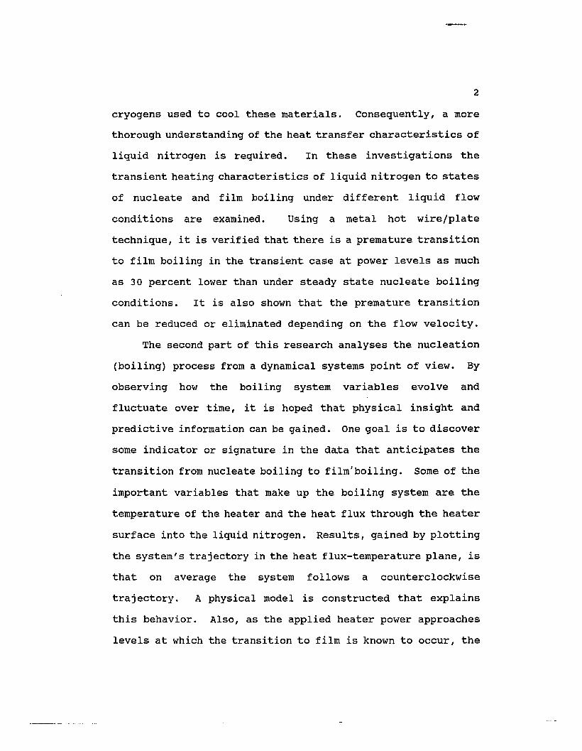
2

cryogens used to cool these materials. Consequently, a more

thorough understanding of the heat transfer characteristics of

liquid nitrogen is required. In these investigations the

transient heating characteristics of liquid nitrogen to states

。f nucleate and film boiling under different liquid flow

conditions are examined. Using a metal hot wire/plate

technique , it is verified that there is a premature transition

to film boiling in the transient case at power levels as much

as 30 percent lower than under steady state nucleate boiling

conditions. It is also shown that the premature transition

can be reduced or eliminated depending on the flow velocity.

The second part of this research analyses the nucleation

(boiling) process from a dynamical systems point of view. By

。bserving how the boiling system variables evolve and

fluctuate over time , it is hoped that physical insight and

predictive information can be gained. One goal is to discover

some indicator or signature in the data that anticipates the

transition from nucleate boiling to film/boiling. Some of the

important variables that make up the boiling system are the

temperature of the heater and the heat flux through the heater

surface into the liquid nitrogen. Results , gained by plotting

the system's trajectory in the heat flux-temperature plane , is

that on average the system follows a counterclockwise

trajectory. A physical model is constructed that explains

this behavior. Also , as the applied heater power approaches

levels at which the transition to film is known to occur , the

3

area per unit time swept out in the heat flux-temperature

plane is seen to reach a maximum. This could be of practical

interest as the threshold to film boiling can be anticipated

and possibly prevented.

ACKNOWLEDGEMENTS

The culmination and success of this work is largely due

to the efforts of people other than myself. At this time I

would like to thank those that have had a large influence on

my indoctrination and socialization as physical scientist.

First , I would like to thank my advisor , Dr. Erik Bodegom

for his help in all facets of my education in the

laboratory. His patience with the lab neophyte who scarcely

knew the difference between an op-amp and an oscilloscope

was appreciated. Also , his knowledge of both experimental

and theoretical concerns provided a broad base for me t。

draw on and gave me a wider scientific perspective. More

importantly though , through our similar perspectives and

shared sense of humor , I hope we remain friends long after

my stint at psu.

As the veteran experimentalists in the lab , Dr. Laird

Brodie ’ s insight and skepticism into the techniques and

results of my work kept me thinking and honest.

As our labs "resident theoretician" Dr. Jack Semura

provided enthusiasm, new ideas and perspectives on projects.

It would be fair to say he introduced "chaos" to our lab!

I would also like to thank the Science support Shop for

building and repairing many of the apparatuses used in the

experiments. Specifically, Brian McLoughlin and Lee Thannum

1V

for help and instruction in the electronics (Brian must have

replaced at least one transistor for each device that I

even thought of turning on) and Rudi Zupan and Gar。

Arakelyan for their skills in machining and constructing the

mechanical devices.

I would also like to thank my parents who , though n。

fault of their own , raised a scientist. They

enthusiastically supported all facets of my education ,(though they began to wonder why it took me over 25 years t。

become educated. Maybe it was too many Grateful Dead

concerts?)

Lastly , I would like to thank my wife Kirsten for

supporting my plans to attend graduate school and putting up

with my protracted education until I could finally obtain a

"real" job. Though she still isn't quite sure just what it

is I do everyday , at least now I will get paid to do it.

ACKNOWLEDGEMENTS

LIST OF TABLES

LIST OF FIGURES

TABLE OF CONTENTS

PAGE

1.1.1.

V 1.1.

V 1.1.1.

CHAPTER

I

II

工II

IV

v

VI

VII

INTRODUCTION . . . . . • . . . . . . . . • . . . 1

BASICHEAT TRANSFER CHARACTERISTICS . . • . • . 8

EXPERIMENTAL PROCEDURE •..•••.•.••.. 13

Dewars • • • • . . . . . . . • • . . . • . 13

Heaters/Thermometers . • . . . . • . . . . 14

Electronics • . • • • • • . • . • . • . . 19

Flow Apparatus . • • . • . . • • . • •• 21

RESULTS AND DISCUSSION • . • • • . • •• ••. 23

Platinum Wire Results . • • . . • . • . • 24

stainless Steel Ribbon Results . • . • • . 34

Dewar Geometry . • • . . . • . . • . .• 41

Summary • . • . . • • • . . . • • • . . • 45

INTRODUCTION TO NONLIMEAR DYNAMICS • . • . • • 47

REVIEW OF RELEVANT DYNAMICAL CONCEPTS . • • • . 53

IMPLEMENTATION OF CONCEPTS IN

AN EXPERIMENTAL SITUATION • • • • • • • • • • • 64

V l.

VI工I DYNAMICAL SYSTEMS RESULTS • . . . • . • • • . • 72

IX

Fourier Transform Results

Phase Space Reconstructions

F‘luctuations in the Q-T plane.

Summary. . . .

CONCLUSIONS

.73

76

7.9

86

89

REFERENCES

APPENDIX

.92

.96

TABLE

I

LIST OF TABLES

Power Leyels for Various Configurations(in W/cm~)

PAGE

• 38

II Peak Heat Fluxes as a Function。f Dewar Geometry (in W/cm2). • • • • • • • • • 44

FIGURE

1.

LIST OF FIGURES

Equipment Schematic .

PAGE

• 15

2. Superheat Temperature AT vs. Time

without Forced Convection . • • • . • . • • . • 26

3. Superheat Temperature AT vs. Time

without Forced Convection

4. Superheat Temperature AT vs. Time

with Forced Convection

5. Heat Flux Q vs. Time

• .28

•...••. 31

without Forced Convection . • . • . . . . • • . 32

6. Heat Flux Q vs. Time

with Forced Convection

7. Superheat Temperature AT vs. Time

.33

without Forced Convection . . . • • . • . . • • 35

8. Superheat Temperature AT vs. Time

9.

10.

11.

with Forced Convection_tr

수뜨- vs. Wire Velocity v . . •Pcrit

Dimension as a Scaling Parameter.

H응non Attractor

• • • • • .37

• 43

59

• 61

12. Ln of Correlation Length vs. Ln of Box size

for the Henon attractor

13. Phase Space Reconstruction of a Time Series

by the Method of Delays

63

68

FIGURE

14.

15.

16.

17.

18.

19.

20.

21.

J.X

PAGE

Amplitude of the Fast Fourier Transform of

the Temperature Fluctuations. . • . . • . • • .74

Amplitude of the Fast Fourier Transform of

the Heat Flux Fluctuations. . • . • . . • • . .75

Ln of Correlation Length vs. Ln of Box size

for the Temperature Fluctuation data. • . • . . 77

Fluctuations about the Steady State

in the Heat Flux - Temperature Plane. . • • • .81

Life Cycle of a Bubble in the

Heat Flux - Temperature Plane . • • . • . . . . 83

Area per unit Time Swept out

in the Heat Flux - Temperature Plane • • • • . .87

Schematic of bubble generator • • • • • • • • • 98

Time Between Bubble Departures vs.

Bubble Number 101

CHAPTER I

INTRODUCTION

Heat transfer is ubiquitous in both nature and any

industrialized society. In the environment , the radiant

energy of the sun is what drives the weather patterns and

consequently the evolving ecosystems. In industry , almost

all processes involve the generation of heat , whether it be

intentional as part of the manufacturing process or merely

as a byproduct required by the second law of thermodynamics.

Indeed , many of the limitations of technological or

industrial applications are due to the generation of heat

coupled with a lack of means to dissipate it effectively.

This can strain the efficiency of many processes and

consequently underutilize precious human and natural

resources. I have decided to study boiling heat transfer in

liquid nitrogen.

At first glance , it appears that liquid nitrogen does

not have much relation to the environment or availability of

resources. But liquid nitrogen's relationship is more

subtle in that it will facilitate enabling technologies

which will have a direct relationship to environmental

concerns. A similar but much more striking analogy is the

computer. By itself it is just some electronic wizardry ,

2

but now in the hands of researchers it is used to model ,

。ptimize ， and understand processes that are of environmental

concern. Stated below are some of the reasons that liquid

nitrogen is increasin당ly important.

with the discovery of the new high critical temperature

(high Tc) superconductors , as well as the increasing use of

cryo-cooled conventional electronics , the use of liquid

nitrogen as a coolant will expand significantly. The

reasons for this are as follows. The new ceramic

superconductors have their superconducting transition

temperature near 120 K, and for these superconductors t。

have electrical characteristics that are stable with respect

to temperature variations they need to be cooled to values

approximately two thirds of the transition temperature.

Therefore a cooling liquid that has its boiling point at tw。

thirds of this temperature is necessary [1]. Liquid

nitrogen (LN2) has a boiling point at one atmosphere of 77 K

so it satisfies that requirement.

It has been found that many conventional semiconductor

devices have enhanced electrical performance when cooled t。

cryogenic temperatures. Such enhancements include faster

switching speeds , lower noise levels and power dissipation ,and greater reliability [2]. Also , there are a number of

reasons besides the low normal boiling point that LN2 is the

preferred cryogen. for both technologies. First , LN2 is a

good dielectric and thus prevents any undesirable electrical

3

interactions with the electronic apparatus being cooled [3].

Second , LN2 is relatively inert , so that there is little

chance that the LN2 will degrade the devices that it cools.

Third , compared to other cryogens , LN2 is a renewable

resource , therefore a virtually unlimited supply of nitrogen

exists. Also , LN2 is generally the least expensive and one

。f the most widely used cryogens in industry.

Therefore , assuming LN2 as the optimal cryogenic

coolant for the majority of electronics applications , a

qualitative as well as quantitative knowledge of its heat

transfer characteristics is required.

In general , systems that involve cryogenic fluids have

not been studied as much as the conventional coolants like

water. One reason is that it has been only in the past few

decades that cryogenic technology has been incorporated int。

industrial applications on a large scale. Though there is

no fundamental physical difference between cryogenic and

noncryogenic fluids (excepting superfluid helium) , the

experiments that one must do are more difficult to perform

because of the necessary cryogenic environment [4].

Finally , a theoretical analysis of solids or fluids at

cryogenic temperatures is more difficult to perform because

。f the often strong temperature dependence of their physical

properties such as the heat capacity and the thermal

conductivity [5].

The system chosen for this investi딩ation involves heat

4

transfer from a solid into the cryogen liquid nitrogen ,under steady state as well as transient conditions. The

primary mode of heat transfer investigated is boiling , as

this is the dominant mode for the heat fluxes anticipated in

applications. Properties studied include the peak steady

state nucleate boiling heat flux and the maximum temperature

to which the liquid can be superheated before boiling

。ccurs. Nucleate boiling is the process of evaporation

associated with vapor bubbles in liquid. Superheating is

the process of raising the temperature of the liquid above

its normal boiling point. A superheated liquid is a

thermodynamically metastable state. It has been shown that

these values can vary depending on the way in which heat is

applied to the liquids. Specifically , for abrupt step

increases of applied power , the maximum allowed power before

film boiling occurs can be as little as 40용 。f the maximum

peak steady state nucleate boiling heat flux [6]. (Film

boiling is a form of boiling heat transfer in which an

insulating vapor film is formed between the heater surface

and the liquid.) This effect is called a "premature"

transition to film boiling. This premature transition t。

film boiling could be an important consideration in the

design of heat transfer systems. For example , transient

heating may induce film boiling thus preventing efficient

cooling of the device and result in burnout of expensive or

critical components of a system. Previous work by Sinha et

5

al indicates that the reason for its occurrence is the lack

。f a well developed natural convection current [6]. The

driving force for natural convection is the heat input

itself. In transient heating this convection current does

not have time to build up to its steady state value , hence

the premature transition. However , the study of Sinha et al

did not give useful quantitative data. In this study, such

data are generated by creating forced LN2 convection. The

results show that in some cases , with flow velocities up t。

50 cm/s , the premature transition can be suppressed for

power levels approaching that of the steady state peak

nucleate boiling heat flux [7]. It should be pointed out

that this premature transition to film boiling was not

。bserved by Giarratano [8] , but several differences between

the experimental conditions of Giarratano and Sinha exist.

The differences are in the ambient pressure and temperature,the wire diameter , and the heat leak into the dewar.

In this research I intend to clarify and define the

limits within which liquid nitrogen can be used as a coolant

for heat generating devices. This dissertation is divided

into two parts. The first part deals with measurements of

temperature and heat flux under conditions of steady state

and transient heating. The second part is an analysis of

the steady state measurements from a dynamical systems point

。f view to see whether any predictive information can be

gained.

6

In this first part I use a standard approach to heat

transfer problems. A thin wire or a flat plate immersed in

a bath of liquid nitrogen is heated and the temperature as a

function of time is recorded. By also recording the applied

heater power , the heat flux into the liquid is calculated as

a function of time. The maximum values of these quantities

that occur are of primary concern , as one is often

interested in the question: "How much heat must be

dissipated before the device fails to work properly or self­

destructs?" The maximum temperature and heat flux attained

have different importance for conductors , superconductors ,and semiconductors.

For example , one does not expect superconductors t。

generate any heat as they have no D.C. electrical

resistance. However , in a type 2 superconductor magnetic

flux lines (fluxoids) penetrate into the superconductor and ,

as a result of their unpredictable motion , generate heat.

At the point or region where the fluxoid moves there will be

some small amount of heat generated. Under A.C. current

conditions the phenomenon is aggravated and the conductivity

becomes finite [9]. Another source of heat generation is

due to the extreme mechanical stresses that can occur in a

superconducting magnet assembly. There , the forces induce

movement of the coil wires and frictional heating results.

The critical factor in all the above circumstances is that

the heat be conducted away before it causes a local

7

temperature rise of the superconductor above its transition

temperature. Otherwise , the resistive portion of the

material could grow and the resultant Joule heating could

destroy the device.

For conventional semiconductor chips the average power

generated can be quite high. In fact , one of the limiting

factors in preventing higher chip densities or higher clock

speeds is the problem of heat dissipation , since

insufficient heat removal is highly correlated with

premature failure [3].

Experiments in this dissertation were designed in view

。f the different requirements of these superconductor and

semiconductor systems. Heat transfer characteristics from a

solid to LN2 are studied under various conditions. The

specific conditions varied were:

1) steady state and transient heating power;

2) forced flow of the liquid or a stationary bath;

3) different dewar geometries;

4) geometries and materials for the heater.

My results indicated that all the above conditions have a

significant effect. The lack of carefully specifying the

above conditions may be the reason for the large range of

values for the maximum nucleate boiling heat flux of liquid

nitrogen that have been reported in the literature [10].

CHAPTER II

BASIC HEAT TRANSFER CHARACTERISTICS

In this Chapter- I describe some of the relevant

concepts , vocabulary and mechanisms involved in the study of

heat transfer. Heat transfer is known to occur in several

modes. These different modes are conduction , convection ,

radiation , and boiling [11]. Conduction heat transfer is

due to the interatomic interaction of molecules i.e. ,

sharing of energy through collisions when a temperature

gradient exists in the medium. This can occur in any phase

。r type of material. Convection is a form of heat transfer

that can only occur in a fluid (gas or liquid) in a

gravitational field. This occurs when a temperature

gradient causes the density of the fluid to vary in

different parts of the fluid. This variation in fluid

density in conjunction with gravity , is the driving force

for the mixing of the fluid. Heat transfer is thus enhanced

。ver pure conduction conditions. Radiation heat transfer

exchanges energy through the electromagnetic field.

However , for this study and the small superheat conditions

under which it was done , radiation heat transfer can be

neglected.

Boiling is different from the above three mechanisms in

9

that the energy transfer primarily occurs through the latent

heat of vaporization of the liquid. That is , energy is

removed from the hot surface when a vapor bubble is formed

from the liquid and then is transported to a cooler

environment where it either collapses back into the fluid or

is vented to the outside atmosphere. Also , due to the

agitation produced by the bubble motion through the liquid

there is some boiling induced convection that occurs. Each

。f these modes is dominant under different conditions , which

are determined by temperature , temperature gradient , ambient

pressure , and type of liquids involved , and so forth [4].

Boiling is generally the most efficient form of heat

transfer in cryogenic fluids. In this study , the stress is

。n conduction , convection , and in particular boiling.

Boiling can be divided into two different categories ,nucleate and film boiling [11]. Nucleate boiling from a

solid surface is commonly what one observes in water.

Bubbles form at particular nucleation sites on the heated

material. The bubbles grow in size and then detach from the

surface when the buoyant forces overcome the cohesive forces

。f surface tension. Typically these sites are microscopic

cracks and crevices in the material that contain "seeds" of

vapor. Nucleate boiling is also called heterogeneous

nucleation because the bubble forms at the interface between

two different substances (e.g. , the liquid nitrogen and the

solid heater material) [12].

10

Film boiling can be considered an extreme case of

nucleate boiling. That is , for increasing heat fluxes , the

bubble formation on the surface of the material occurs s。

rapidly that the bubbles do not have time to detach and be

replaced by liquid. The result is that nearby bubbles

coalesce and a vapor film covers the surface and impedes

further heat transfer due to the insulating effect of the

vapor film. This in turn drives up the temperature

difference between the heat producing object and the

surrounding liquid. The heat flux at which this occurs is

termed the critical heat flux. In liquid nitrogen the

increase in temperature due to film boiling can approach

hundreds of degrees over that of nucleate boiling for the

same heat flux. Such a large temperature increase is

usually detrimental to the heat producing device and thus

should be prevented. The critical (or peak) heat flux is

the maximum attainable heat flux just before the transition

from nucleate boiling to film boiling occurs. This heat

flux is achieved by slowly increasing the heater power until

film boiling occurs [13].

Contrasted to heterogeneous nucleation is homogeneous

nucleation in which the vapor "seed" originates in the bulk

。f the fluid and not at the interface between liquid and

solid [14]. It is known that a liquid can withstand a

certain amount of superheat (i.e. , heated above its normal

boiling point) in the absence of external initiating

11

influences , before a transition to the vapor phase takes

place. In a pure liquid such as nitrogen , this superheat

approaches several tens of degrees [15]. The transition

。ccurs when a sUfficiently large number of vapor nuclei ,

induced by thermodynamic fluctuations in the liquid , reach a

critical radius and grow spontaneously in the liquid. This

causes the very rapid formation of many bubbles in the

superheated liquid adjacent to the wire. The spontaneous

initiation of homogeneous nucleation and the sUbsequent

cooling effect restricts further increases in the

temperature. Although the temperature at which this occurs

is not defined precisely , the kinetic theory of homogeneous

nucleation predicts the nucleation rate to depend

exponentially on parameters related to the degree of

superheat [14]. Thus in practice a relatively sharp

superheat maximum is attained. For LN2 this temperature is

110 K at 1 atmosphere.

It also appears that how the heat flux is applied can

have an effect on the critical heat flux. Some authors have

found that for sudden step increases of power application

the maximum allowed heat flux before film boiling occurs can

be as little as 40웅 。f the critical heat flux [6]. This

effect is called a premature transition to film boiling.

Note that under slightly different experimental

conditions , this phenomena was apparently not observed by

。ther investigators [8]. Thus , there still is a question as

12

to the existence of this phenomenon and under which specific

conditions it occurs.

In this study I investigated nucleate boiling and the

conditions under which the transition to film boiling occurs

in liquid nitrogen. I thus sought to clarify the occurrence

。f the premature transition to film boiling and investigate

methods to reduce , eliminate , and/or predict the transition

to film boiling.

CHAPTER III

EXPERIMENTAL PROCEDURE

A brief synopsis of the experimental setup is given

here. More detailed sUbsections follow. The experiments

were conducted in dewars of varying sizes and geometry.

Also , heaters and thermometers of different materials and

geometry were tried. Measurements of the voltage and

current signals were made to determine temperature and

applied heater power. Forced convection was achieved by

moving the heater through the stationary liquid in the

dewar. Finally , a computer was used to automate the

experiments and digitize the data for later retrieval and

analysis.

DEWARS

The experiments were conducted in cylindrical dewars

vented to atmospheric pressure. The capacity of these

dewars varied from 1 to 35 liters. The diameter and length

respectively for these dewars were 7 by 30 cm (glass) , 5 by

50 cm (glass) , and 35 by 40 cm (steel). One configuration

had the smaller of the glass dewars inserted into the larger

。ne so that better insulation could be achieved. Because of

the variability of insulation in the dewars , heat leak int。

14

the containers caused the bath of nitrogen to vary from a

very quiescent state as in the in the steel storage dewar t。

。ne of steady boiling which occurred for the smaller glass

dewar.

HEATERS/THERMOMETERS

Three different geometries for the heater/thermometer

were used. The first heater/thermometer assembly used was

composed of a 8 cm length of platinum wire 0.1 mm in

diameter (See Figure 1). To minimize the effect of heat

loss by conduction through the two voltage leads , fine wires

were used as the voltage sensing leads , and were soldered

1.5 cm from each end of the wire. Thus the effective

thermometer length was 5 cm [16]. The other tw。

heater/thermometer assemblies used were composed of a 6 cm

length of "302" stainless steel ribbon 0.05 mm thick and 0.2

and 1.0 cm width. Similar precautions to prevent heat leak

through the voltage and current leads were taken. These

geometries were chosen because they are similar to those

which are found in electronics applications utilizing wires

and integrated circuits. The heater surfaces were oriented

vertically in the dewar. The two primary measurements made

were the temperature and the heat flux into the liquid , both

time dependent quantities.

The method of heat generation and temperature

measurement was accomplished by the same instrument and is

Voltageμads I r I Current μads

pt Wire

15

/Glass Tube

cu Wire

Spring

Fiaure 1. Equipment schematic. Upper diagram isplatinum heater thermometer. Lower diagram iscircuit schematic for experimental control anddata acquisition.

16

known as hot wire thermometry [17]. The basis for this

technique is essentially resistance thermometry , with the

additional function that the material used to measure the

temperature is also the one that generates the heat flux

into the medium. This alleviates the problem of imprecise

determinations of the temperature and heat flux when the

heater and thermometer are spatially separated. The heating

current (a few amperes in the case of the platinum and tens

。f amperes for the steel) was controlled by an

。p-amp/transistor array described in the next section.

The temperature change of the heater as a function of

time was determined by measuring the resulting change in

electrical resistance of the heater since the electrical

resistance is a well characterized property of a metal. In

particular, the electrical resistance is a monotonically

increasing function of the temperature that typically has a

linear dependence on the temperature over a narrow

temperature range. However , some metals are more strongly

temperature dependent (i.e. , they posses a larger

temperature coefficient) than others , and some are closer t。

linear in their temperature dependence than others. These

properties determine the sensitivity with which the

temperature can be measured and the ease in calibrating such

a device. The metals used were platinum and stainless

steel , of which the former has the most linear and largest

temperature coefficient of the metals. At 77 K platinum's

17

resistivity changes 2 옹 per degree. Both metals have

temperature coefficients that are very stable over time and

it do not react readily with other substances. The

temperature coefficient of both platinum and stainless steel

were very close to linear in the temperature range of

interest , so the calibration method was to record resistance

measurements at the two temperature extremes and

interpolate. The two end points chosen were the saturated

bath temperature Tbl (77.3 K @ 1 atmosphere pressure) and

room temperature (293 K). The temperature coefficients

calculated were checked against handbook values and found t。

agree within 5 percent [18]. To calculate the temperature ,

a known current was passed through the material.

Simultaneously , measurements of the voltage difference

between two points of the "resistor" were made. From these

measurements one calculated the resistance using Ohm's law,and thus the temperature.

Another consideration is that the measurements of the

temperature and heat flux are transient , so that the

thermometer had to be able to track rapid temperature

changes. That is, the heater thermometer had to be in

thermal equilibrium with the liquid immediately surrounding

it at times scales on the order of a millisecond. This time

scale was determined by observation of nucleate and film

boiling processes at the heat flux levels of interest in

this study. The thermal response time is a function of the

18

material and its geometry , and was calculatedby the

following equation.

r: =d2/K

where

K=k/pc

(1)

(2)

and d is a characteristic dimension of the material , such as

the thickness of the wire or the ribbon. κ is the thermal

diffusivity , k is the thermal conductivity , p is the

density , and c is the specific heat. For the platinum wire

and the stainless steel ribbon the time constants were

60 μsand 500 μs respectively. Note that these

thermophysical properties changed with temperature , but that

in the temperature changes encountered (20 degrees celsius) ,this amounted to less than a 15옹 change in the time

constant.

The overall uncertainty in determining the heater

temperature had two contributions. First , was determining

the superheat temperature , that is the temperature changes

relative to the ambient bath temperature. This uncertainty

was effectively a function of the precision with which the

current , voltages , resistance , temperature coefficient , and

amplifier gains could be determined. This uncertainty was

estimated to be no more than 0.3 degrees celsius over a 20

degree temperature span. There was an additional

.uncertainty due to the precision that the saturation bath

19

pressure was known and the ability to electronically

subtract out the corresponding ambient bath temperature

value from the signal. This was estimated to be 0.3 degrees

celsius as well. However , the sensitivity , which was

determined by the effective length of the heater/thermometer

and the noise in the electronics and environment , was of the

。rder of millikelvins.

The limiting factors in determining the overall

accuracy in heat flux were the precision of the current ,resistance , and the geometric measurements for the material.

The accuracy for the heat flux was found to be 5옹.

ELECTRONICS

The circuit schematic for the metal heater/thermometer

and the associated electronics is shown in Figure 1 and

described below. The output of a pulse generator or a D.C.

voltage source , was sent to a current amplifier which was

configured to supply a constant current to the

heater/thermometer. In series with this were two 100 watt ,0.25 ohm resistors. These resistors had a low temperature

coefficient so as to minimize heating errors when reading

large currents. Instrumentation amplifiers 1 and 3

amplified the voltage V깐 (t) across the platinum wire Rpt;'

and the voltage VI across resistor R3 respectively. Rpt; can

be thought of as being composed of two contributions , a

temperature independent term called R01 and the temperature

20

dependent term called ~R(T). On an absolute scale the

temperature coefficient of metals were small and thus the

majority of the measured signal of Vpt(t) was due to the

temperature independent part of the resistance ROI and was

called~. Frequently one is interested in the superheat

temperature ~T(t). The temperature changes about the

normal boiling point (i.e. for LN2 , ~T(t) = T(t) -77.3 K).

Therefore , in order to produce a signal reflecting only the

superheat temperature , the constant portion VO must be

electronically subtracted from VPt (t) to yield ~ T( t). This

was accomplished by manually adjusting the gain from

amplifier 2 so that the output of amplifier 4 is zero when

no superheating has occurred. This balancing procedure was

implemented when the heater/thermometer was known to be at

77.3 K as is the case at the very beginning of the current

pUlse. The signals from amplifiers 3 and 4 were then

recorded on a digital oscilloscope. Then the digitized data

were stored in the computer for further manipulation.

The equations to solve for the superheat temperature

~ T( t) follow.

V깐( t) = Vo + ~ V ( t) = I RPt = I (Ro+~R ( t) )

V상 (t) =IRo(1+ α~T( t) )

(3)

(4)

• 21

Solving for AT( t) gives

_ AR(t) _ (v깐 (t) -IRa) / IAT(t)= ... .n\f.,'_

Ro« R。 α(5)

where V상 (t) was the voltage difference between two points

。n the heater/thermometer , ~ was the voltage due t。

the temperature independent part of the resistance Roo

VI was the voltage across the 0.25 ohm resistors and was

directly proportional to the current I through the

heater/thermometer , α was the temperature coefficient for

the particular metal and AT(t) was the calculated superheat

temperature above 77.3 K.

FLOW APPARATUS

In order to enhance heat transfer one common technique

is to use forced convection. Forced convection was achieved

in this work by moving the heater/thermometer either up or

down in the dewar by means of a variable speed DC electric

motor. The reason for moving the heater/thermometer rather

than generating a flow of liquid nitrogen is that the motor

induced flow was easier to measure and control. The

apparatus was assembled as follows. An electric motor had a

round gear at one end of its drive shaft. This gear meshed

with a rigid linear rack (approximately 50 cm long) oriented

vertically. The rack was held in place by idler wheels and

。nly allowed to move in the vertical direction. Attached t。

the bottom of the rack was the heater/thermometer assembly.

22

Thus there was just under 50 cm of vertical travel. with

the particular gear ratios , motor assembly , and dewars

utilized , maximum velocities of 50 cm/sec were possible.

The velocity was determined by a photogate timer which

measured the time which a 1 cm vane attached to the

heater/thermometer shaft took to pass through the photogate.

The uncertainty in controlling and determining the

velocity was due to two factors one; the ability to regulate

the current to the electric motor , and two , the resolution

with which the vane geometry and timer measurements could be

determined. I measured the variation in these parameters

and found the overall uncertainty in velocity is 6 percent.

Both the movement of the heater/thermometer assembly

and the heating current through it were controlled and

coordinated by a computer. A typical run proceeded as

follows. First , the computer sent a signal to initiate the

flow. Second , after allowing sufficient time for the flow

to stabilize (0.2 sec) the heater/thermometer was pUlsed

with current (typically for 0.65 sec) and the resulting

signals were recorded on the digital oscilloscope. Third ,the flow was stopped , and the oscilloscope sent the

digitized traces to the computer for storage. The

thermometer assembly was backed up to its original position.

This sequence was then repeated after 2 minutes to allow the

LN2 to settle down. For each applied power setting and

velocity , several runs were taken to insure reproducibility.

CHAPTER IV

RESULTS AND DISCUSSION

The only two measurements that were made durin당 a "run"

were the voltage across the heater/thermometer and the

current through it as a function of time. From these data

。ne could calculate the resistance , and thus temperature of

the wire , the total power dissipated in the wire , and the

total heat flux out of the wire and into the liquid. This

first section describes how the heat flux analysis was

performed (the temperature calculation was explained in

Chapter III).

The heat flux O(t) , is not simply the total power

dissipated per unit area , as was the case for steady state

heat flux experiments. There is a correction term due t。

the non-zero heat capacity of the wire. This is given by

the following equation.

dTp( t) =O( t) +C ~~dt

(6)

where C is the heat capacity per unit surface area of the

wire and pet) is the total applied power per unit surface

area of the wire (ie. 12R(t)/A). The applied power

increased with time since the resistance of the wire is

increasing with temperature. This was accounted for when

24

the calculation of P(t) were made on the computer and

plotted. However , references made to different heating

curves indicate their initial power dissipation at t=O.

Since the temperature of LN2 is significantly below the

Debye temperature of platinum and stainless steel , the heat

capacity varied significantly as a function of temperature.

This was adjusted accordingly when the calculations are

made. dT(t)/dt is the time rate of change of the

temperature of the wire and this was obtained numerically.

Thus it is seen from Eqn. 5 that because of the non-zer。

heat capacity , in the transient case the heat flux into the

fluid could be greater than or less than the applied power.

In the true steady state case the two are equal.

In addition to the transient measurements mentioned

above , measurements were also made to determine the peak

steady state heat flux. As a reference, the maximum value

。f the steady state peak heat flux for the three heaters was

9.5 w/cm2 • This was for the platinum wire heater surface.

Peak steady state heat flux values lower than this were als。

。btained and it is shown later that these values depend on

the dewar and heater geometry. The figures and discussion

were separated on the basis of the heater material.

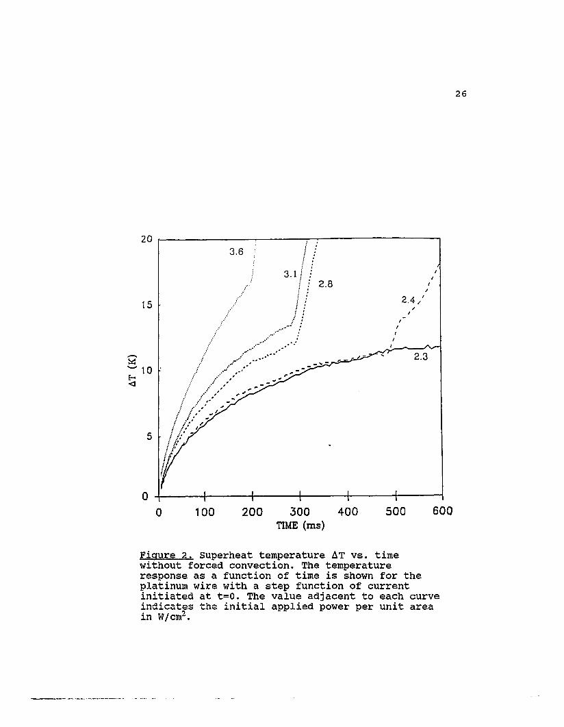
PLATINUM WIRE RESULTS

Figure 2 shows the superheat temperature vs. time under

no flow conditions. The figures were labeled in terms of

25

the initial applied power. This was done to provide a

reference since in these constant current experiments the

resistance was increasing with temperature and thus the

power level increases as well. For an initial applied power

。f 2.3 W/cm2 the temperature rose steadily. At this

particular current the onset of nucleate boiling occurred

after 600 ms , after which the temperature of the wire drops

to 4 kelvins above the bath temperature. At a slightly

larger power (2.4 w/cm2 ) a transition to film boiling occurs

as could be observed by the abrupt increase in the slope of

the temperature-time curve at 450 ms. This transition is

called premature because the transition to film boiling

。ccurred at power levels less than the peak steady state

nucleate boiling heat flux of 9.6 w/cm2 • When the effect of

the increased resistance was included in the heat flux

calculation , the premature transition to film boiling was

seen to occur at nearly 30옹 。f the peak nucleate boiling

heat flux. At even higher power levels the transition t。

film boiling occurred at earlier times and higher superheat

temperatures were reached before film boiling commences.

Figure 3 shows the nucleate boiling stage in more

detail and from a different data set. For comparison , a

heating curve (curve A) is included which shows the

theoretical result for a wire with constant power

dissipation. It was assumed that only conduction occurs and

that there is no temperature gradient in the wire. This

203.6

15

/

/

2.4//

/

/

."、..-‘

엌

-10E-o<1

5

·nunu

100 200 300 400TIME (ms)

500

Fiqure 2. Superheat temperature AT vs. timewithout forced convection. The temperatureresponse as a function of time is shown for theplatinum wire with a step function of currentinitiated at t=O. The value adjacent to each curveindiεat?s th승 initial applied power per unit areain W/cm~.

26

600

27

latter assumption was justified because platinum's thermal

conductivity is nearly 600 times greater than LN2. In this

case the analytical solution is given by [19]:

1ttu Z

T( t) =죠앞: r (1-e fa )u-3du ‘

π3K { [uJo ( 띠 -«J1 ( 띠]2 + [uYo (u) -«Y1 (u) ]2

where

20 •••~cα _ .... t" LN2 ....LN2-----­Ppt; C pC

(7)

(8)

is a parameter which is twice the ratio of the heat capacity

。f an equivalent volume of the medium (LN2) to that of the

conductor (platinum). It is 1.74 at 80 kelvins. K is the

thermal conductivity of the LN2 , and q is the heat generated

per unit length of the wire. K is the thermal diffusivity

for the LN2 defined earlier (Equation 2). The radius of the

wire is denoted by a. Jo(u) and J1(u) are Bessel functions

。f the first kind , of order zero and one respectively.

YO (u) and Y1 ( 비 are Bessel functior뀐 。f the second kind , of

。rder zero and one respectively. For a short time it can be

seen that the analytical curve and the experimental curves

agree. When the experimental curves begin to diverge from

the analytical one , modes of heat transfer other than

conduction are commencing.

The three other curves (curves B,C,D) were from

experiments under "identical" conditions of an initial

applied power of 3.7 w/cm2 and without forced convection.

28

3.7 W/cm2

20

10

5

15

(올)←김

500400200 300TIME (ms)

100

oO

3.7

Fiqure 3. Superheat temperature aT vs. timewithout forced convection. The temperatureresponse as a function of time is shown for theplatinum wire with a step function of currentinit~ated at t=o. The initial applied power isW/cm‘.

29

Curve A began to deviate from the others at approximately 50

milliseconds. The three experimental curves also initially

coincide but at 50 milliseconds began to separate. After

approximately 100 milliseconds nucleate boiling is well

developed as seen by the smooth decrease in temperature.

The temperature of the surrounding fluid finally reduces t。

approximately a 4 degree superheat. The difference between

the maximum temperature superheat (12 degrees) and the

steady state nucleate boiling superheat (4 degrees) is

called "overshoot". The value of this overshoot is an

important design criterion for superconductors , as one wants

to prevent the critical temperature from being exceeded or

wide temperature variations from occurring. Overshoot is

due to a lag in the onset of steady state nucleation at the

surface of the wire. That is , initially all the nucleation

sites are not active. This hysteresis effect is common in

the cryogenic fluids because they wet surfaces very well and

significant superheats are often required to activate them.

One other feature that stands out in the three

experimental curves in Figure 3 is that the curves deviated

from one another between 100 and 400 ms. This was typical

for data collected under "identical" conditions. The origin

。f this variation was that the experiment is not done under

equilibrium conditions. Because the definition of

superheating a liquid is to bring the liquid into a

metastable state, the higher the superheat the farther from

30

equilibrium the system is and thus the system is

increasingly unstable. This instability makes the system's

evolution extremely sensitive to the initial conditions.

For example , a slight difference in the temperature profile ,the convection pattern , or even a stray bubble in the liquid

might make a difference as to which path the system

"chooses".

Figure 4 emphasizes the aforementioned instability of

the system and shows that under "identical" conditions of

flow and applied power the system either went into nucleate

boiling or film boiling. Thus these initial conditions

appear to be on the dividing line between the two routes the

system can take.

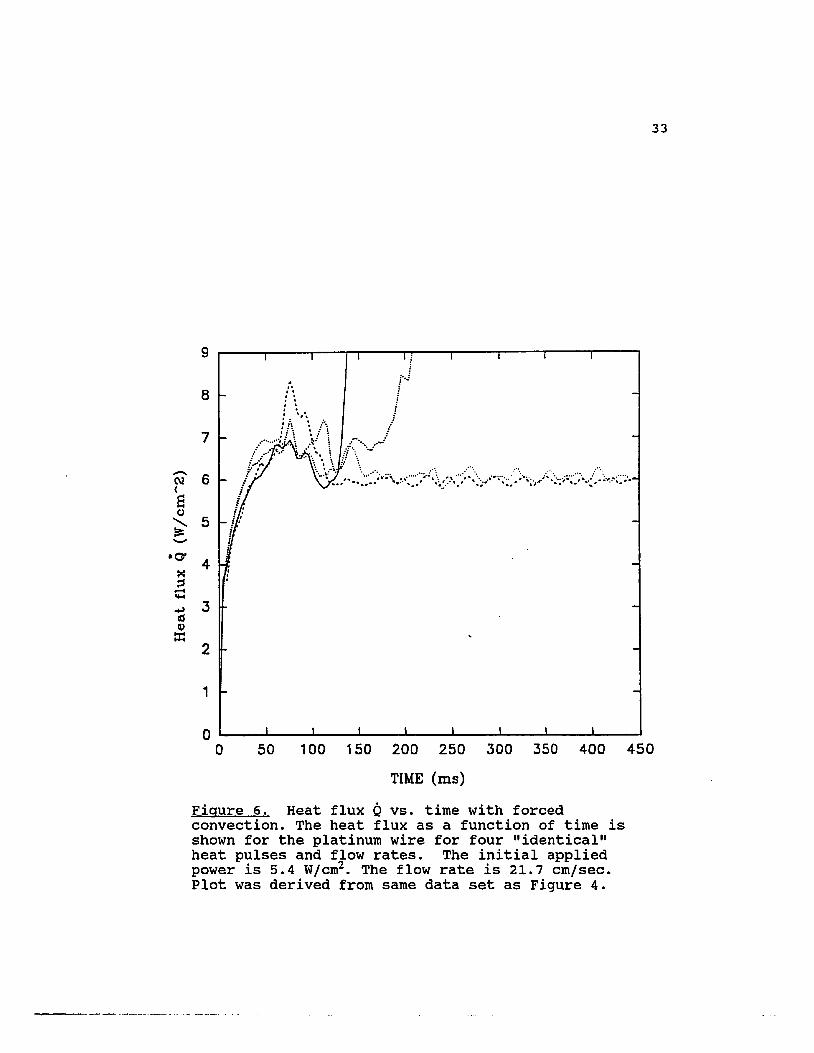
Figures 5 and 6 are from the same data sets as Figures

3 and 4 respectively. However , these show the calculated

heat flux Q(t) vs. time curves as discussed previously.

These curves also appear to follow similar paths for a short

time and then separate. The abrupt heat flux peaks in

F’igure 6 indicate that vapor formation is occurring , thus

cooling the superheated liquid. As long as the vapor

formation does not occur too quickly and extensively film

boiling did not occur. It is seen that the two curves that

go into film boilin당 achieved a higher superheat , and

consequently were more unstable. Also note in these plots ,prior to film boiling , the transient heat flux never

exceeded the steady state value. In fact , the transition t。

31

20

15

ι-、

닙

-10ε‘<I

5

, ..-‘‘‘‘--‘ ......‘... _.........,.‘ , “ .-‘ “ .

--_... ‘ . .• ‘ ..... ~ - ...‘· ‘. ‘

‘ ---",- .... _-，，-、 .......... -_ .... “，，-、" -‘-‘-------시--

oo 50 100 150 200 250 300 350 400 450

TIME (ms)

Fiqure 4. Superheat temperature AT vs. time withforced convection. The temperature response as afunction of time is shown for the platinum wirefor four "identical" heat pulses and flow rates.The initial applied power is 5.4 W/cm~. The flowrate is 21.7 em/sec.

32

6

5

(\)N，‘놀g。 4

3.cy

{얻μni}

‘얼6@ ,‘

·0o 50 100 150 200 250 300 350 400 450

TIME (ms)

Fiaure 5. Heat flux Q vs. time without forcedconvection. The heat flux Q as a function of timeis shown for the platinum wire with a stepfunction of current initiated at t=O. The initial

’applied power is 3.7 W/cm~. Plot was derived fromsame data set as Figure 3.

33

9

8

7

(\)N‘톨gQcuS니

·c[‘’pr‘ -

}북@@3

2

oo 50 100 150 200 250 300 350 400 450

TIME (ms)

Fiaure 6. Heat flux Q vs. time with forcedconvection. The heat flux as a function of time isshown for the platinum wire for four "identical"heat pulses and fJow rates. The initial appliedpower-is 5.4 w/cm2 • The flow rate is 21.7 cm/sec.Plot was derived from same data set as Figure 4.

34

film boiling occurs at power levels nearly 30웅 。f the steady

state value. This is the premature transition to film

boiling referred to earlier. Moreover , a specific value of

the transient critical heat flux or the superheat

temperature for which film boiling inevitably occurs does

not appear to exist. This suggests that other degrees of

freedom are necessary to specify the state and evolution of

the system.

STAINLESS STEEL RIBBON RESULTS

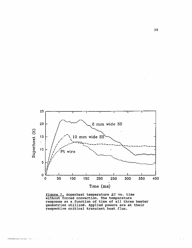
Qualitatively , the superheat vs. time curves for the

stainless steel looked similar to the platinum wire curves.

See Figure 7 for a comparison of the three

heater/thermometers used. These curves were at power levels

corresponding to their peak transient nucleate boilin당 heat

flux , 。r p:git- p잖it is defined as the maximum heat flux

level attainable under transient and no flow conditions , in

which film boiling did not occur.

Figure 8 shows the effects of various flow rates at a

fixed applied current for the stainless steel geometry. The

premature transition to film boiling occurs under zero flow

condition at 75 ms and with increasing wire velocities this

transition was delayed. Finally , at a high enough velocity

film boiling was prevented. This pattern of increasing the

delay to film boiling was obtained for higher power levels

as well. However , the maximum one was able to delay film

35

25

/./‘\ 10. \

// ---，〉-‘:~:.~-‘--“，ι 、 ---- -----‘--

/ 一..~’ -‘-、、

ι끼Pl wire 、‘、、1/ \‘’--‘._----1/ 、、-

I ,' 、-、、---

I，'‘-‘-‘t、----( --‘------‘---,-/

ssmm wide20

15

10

5

(성)}φU{한UQjm

400350300때

때/tl‘、

20015010050o

o

Time

Fiaure 7. Superheat temperature aT vs. timewithout forced convection. The temperatureresponse as a function of time of all three heatergeometries utilized. Applied powers are at theirrespective critical transient heat flux.

36

boiling if it was going to occur at all , was a few hundred

milliseconds. Superheat plots and delay times under flow

conditions similar to Figure 8 were also true for the

platinum wire.

Table I gives a summary of the pertinent results on the

various power levels attained for both the stainless steel

and platinum heater/thermometer configurations. The effects

。f flow and transient heating are also included in Table I.

p~휠 t is the critical applied power per unit area under

steady state conditions and no flow. It is also called the

peak steady state nucleate boiling heat flux. This value

was used as the baseline when making comparisons because it

is the one typically quoted in heat transfer studies.

p‘짧x is the maximum power level attainable in which film

boiling did not occur under transient heating and maximum

flow conditions. By looking at the ratios one can determine

the severity of the premature transition to film boiling and

the effect that forced convection had on suppressing it.

The uncertainty in the reproducibility of the heat fluxes is

plus or minus 0.1 W/cm A 2.

The difference in power levels can be understood as

follows. In the case of the thin wire , the bubble size at

departure was equal to , or greater than the size of the wire

diameter. In effect , it only takes one bubble to surround

the wire and initiate film boiling. The probability that

this occurs is greater than if many bubbles

37

42.7

”“--3----‘,3-

/”--ζ

/‘

25

20

15

10

(웅)}며U죄」ωQam 5

40035030025020015010050oo

Time (ms)

F’iqure 8. superheat temperature AT vs. time withforced convection. The temperature response of the2 mm wide stainless steel heater is shown for anapplied power of 8.1 w/cm2 • The numbers adjacentto the curves indicate the velocity of the wire incm/sec.

38

TABLE I

POWER LEVELS FOR VARIOUS CONFIGURATIONS (IN W/cm2)

Heater pcsrsl.t p:휠tp찮t

P~pvtnI펴;

Configuration P~:i.t: p앓l

0.2 cm wide 10.4 6.7 0.70 8.7 0.84steel ribbon

1.0 cm wide 6.3 4.8 0.77 6.7 1. 06steel ribbon

.01 cm 9.6 4.0 0.42 6.6 .69diameterplatinum wire

are required to coalesce into a film. Therefore , fewer

bubbles (ie. lower power levels) were necessary to initiate

film boiling with a thin wire than with an extended ribbon

style heater surface. This mechanism holds whether

transient or steady state heating was occurring. The reason

this argument does not seem to hold for the largest heater

(ie. the 1.0 cm wide heater) was because of other effects

that dominated. These other effects were the confined dewar

geometry in conjunction with the large total power

dissipated into the liquid. The total power dissipated int。

the liquid was greater because of the greater total surface

area of the wide heater. Consequently, visual observations

indicated that much more boiling was occurring in the dewar

than when the platinum wire was used. Because of the

confined geometry , normal convective flow was impeded by the

large high density of bubbles and film boiling resulted at

39

lower heat fluxes. The effect of dewar geometry on the

critical heat flux was not anticipated; however , a more

detailed study was initiated and is discussed in a later

section.

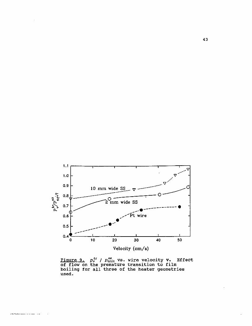
Figure 9 shows the effect of flow on eliminating the_ tx

premature transition to film boiling. The plot is ~똥- vs.Pcrit

wire velocity v for all three of the heater geometries used.

p;I is the maximum threshold power below which the

transition to film boiling never occurred when the wire

velocity is equal to v and p~화t was previously defined. It

is important to keep in mind however , that the power levels

plotted are a lower limit for a particular flow velocity.

These data obviously do not lie on a straight line; it is

not certain whether the data should follow a linear or

quadratic power law. The lines drawn through the data are

to guide the eye and are the results of a graphing routine.

It is not to be implied that these data have been fitted

with some simple polynomial. However , the curves are

approximately parallel , which indicates that the flow has

the same general effect on the various heaters. The actual

values of the flow velocity required to prevent film boiling

can be estimated with a model. Also , it is shown that

gravity does not have much effect on these results because

the same results were obtained regardless of whether the

heater/thermometer was moved up or down through the liquid.

A simple model based on a rigid sphere moving through a

40

viscous fluid of a different density was used to analyze the

forces on the bubbles. It was found that the viscous drag

forces were larger than the buoyant forces due to gravity

(Equations 9 and 10 below). This is true for bubbles whose

radius was smaller than 0.1 mm which was the case when

nucleation commences [20]. In other words , the bubbles were

sheared away from the surface by the viscous forces before

they could grow and coalesce into a film surrounding the

wire. The viscous drag force calculated was based on the

model of a rigid sphere moving through a viscous fluid

having a different density relative to the sphere [21].

Here , the sphere is a vapor bubble of nitrogen and the

viscous fluid is LN2. The drag force is:

Fd =6 π a11 v (9)

where a is the radius of the sphere (bubble) , which was

estimated to be 0.01 em from visual observation , v is the

velocity of the heater/thermometer through the fluid ,and 11 is the dynamic viscosity of LN2 at 77 K (1. 58x10-3

g/cm-sec).

The buoyant force on the bubble is given by

맘= (PflUid-Pb뼈ble) g좋 π a 3 (10)

where P is the density of the different phases (0.807 and

0.004 g/cm3 for liquid and vapor respectively) , a is the

radius of the bubble , and g is the gravitational

’acceleration (980 cm/s~). Calculations were made on the

41

velocity necessary to prevent film boiling at a particular

power level. It was determined that one has to replenish

the liquid near the surface fast enough so that the bubbles

forming cannot coalesce into a film. This amounted t。

moving the wire through a distance equal to its length in

the amount of time required for the stationary wire to g。

into film boiling. For instance , from Figure 2 at an

’applied power of 2.7 W/cm~， it is observed that the time

until film boiling is 250 milliseconds. Since the wire

length is 10 cm , the required velocity is 40 em/sec. This

result is within a factor of two of the experimental data if

。ne extrapolates the curves in Figure 9 to the point such_ tr

that 수뜨- equals one.P다it

DEWAR GEOMETRY

As suggested above the dewar geometry and heat leak

into the dewar affect the values of the critical heat flux

and the severity of the premature transition. The former is

true because the geometry determines the boundary conditions

for any convective flow of the fluid. A confined geometry

tends to restrict fluid and bubble flow away from the heater

surfaces. This facilitates the transition to film boiling

and one expects lower critical heat fluxes for the steady

state case.

The effect of heat leak into the dewar was t。

contribute to the total heat flux (heater input plus heat

42

leak) that the fluid experiences. This enhanced the natural

convection in the bath of LN2 which could aid in preventing

a vapor film from forming. But if the heat leak is severe

it can increase the density of bubbles near the heater and

thus make film boiling more probable. This effectively

reduces the critical heat flux of the heater.

with these effects in mind investigations were made

utilizing dewars with different geometries and having

different insulation properties. The dewars chosen were a

35 liter (40x35 cm) storage dewar , a 1 liter ( 30x7 cm)

diameter glass dewar , and a 9 liter (45x5 cm) glass dewar.

The 9 liter dewar was able to be placed inside a larger

dewar containing LN2 , thus reducing the heat leak

considerably. Transient and steady state measurements

without forced convection were made utilizing the platinum

wire. The results are shown below in Table II. The symbols

are as previously defined. The results confirm the

qualitative discussion above. For example , all the

configurations above except the second one had minimal heat

leak into the dewars. This made for a very quiescent bath

in which the premature transition to film boiling occurred

at low power levels. Note these peak transient heat fluxes

are all about 2.8 W/cm2• The second dewar configuration had

visible boiling and mixing of the liquid occurring. This

caused the peak transient heat flux to be greater (4.1

w/cm2) than the other configurations.

43

5040302010

.\1

?

.\110 mm wide 5~_... \l ••••••••••••••••- (j

0--­

j걱2익rin wide SS~ ----------.~ _....---

........Pl wire."---·--

1. 1

1.0

0.9

”“ειι?;;‘’ 0.80.7

0.6

0.5

0.4o

Velocity (cm/s)

Fiaure 9. p;r / p찮t vs. wire velocity v. Effect。f flow on the premature transition to filmboiling for all three of the heater geometriesused.

44

TABLE II

PEAK HEAT FLUXES AS A FUNCTION OF DEWAR GEOMETRY(IN w/cm2)

Geometry of Dewar P~:it p찮t￡-Jctrrit

p짧t

40x35 cm storage 9.0 2.8 0.31dewar

50x5 cm glass 7.4 4.1 0.55dewar(no LN2 bath)

50x5 cm glass 9.6 2.7 0.28dewar(in LN2 bath)

30x7 cm glass 7.0 2.8 0.40dewar

The steady state peak heat fluxes were affected both by

the geometry and the heat leak into the dewar. The second

configuration because of its large heat leak had many

additional bubbles near the heater surface. This higher

density of bubbles contributed to the lower peak steady

state heat flux. Note that when a LN2 bath was placed

around this dewar (configuration 3) the peak steady state

heat flux is increased to a higher value. It was not s。

clear why the fourth configuration has its steady state

value significantly lower (7.0 w/cm2) than all the others.

From visual observation it did not appear that extensive

boiling was occurrin당. It was possible that the heater

surface was adjacent to the dewar wall and thus preventing

the bubbles from dispersing easily.

45

SUMMARY

The first half of this study attempted to answer some

questions in heat transfer that are of direct interest from

a practical viewpoint. Such questions concerned the

critical heat flux through the heat/fluid interface and the

typical superheat temperatures attained. This research

expanded traditional studies of engineering heat transfer in

a few ways. One , a cryogenic fluid was examined under

transient as well as steady state heating conditions. Two ,the effect of geometry in both the heater and dewar

assemblies was determined.

To summarize the results: Transient heating of a solid

immersed in LN2 was found to cause a significant reduction

in the critical heat flux into the liquid. This reduction

could be to as little as 30옹 。f the peak steady state

critical heat flux. The reason for this reduction may have

been the lack of well developed convection currents in the

liquid; in a transient heating experiment there was not

enough time for the quiescent bath to develop convection

currents. This explanation was further supported by the

。bservation that the dewars having enough heat leak such

that mixing was occurring , had higher peak transient heat

fluxes.

The effect of very thin heater geometries (eg. wires)

was to aggravate the premature transition to film boiling.

One explanation was that the bubble size was equal to or

46

greater than the heater diameter. Thus it only took one

bubble to initiate film boiling.

Experiments utilizing forced convection were done t。

quantitatively determine the equivalent effect of natural

convection. Predictions extrapolated from the results

indicate that flow rates between 0.5 and 1.0 meters per

second were necessary to completely prevent the premature

transition to film boiling. Fortunately , these flow rates

are achievable (for instance from pumps or pressurization)

for most practical situations. Furthermore , the added

complexity of a forced convection system may often be

justified by the more than 200옹 increase in transient peak

heat fluxes. Unfortunately , the apparatus used in these

experiments does not allow testing the 0.5 to 1.0 m/sec flow

rates predicted above.

Boiling heat transfer in a confined geometry similarly

reduced the beneficial effects of any natural convection.

The resultant bubbles were not able to disperse freely and

therefore coalesce into a film more easily.

Overall , these results add significant new data to the

heat transfer literature and indicate that previously

neglected questions in heat transfer are important after

all. Hopefully , this course of inquiry will stimulate

further research.

CHAPTER V

INTRODUCTION TO NONLINEAR DYNAMICS

As mentioned in Chapter I , the second phase of this

research involved the fields of nonlinear dynamics ,dynamical systems and chaos theory [22 ,22]. These areas

have grown dramatically since their "discovery" a few

decades ago and they have applications to nearly all

branches of science and engineerin당. Actually , it was at

the turn of the century that much of the work for these

fields was initiated and developed by the French

mathematician Poincar응. However , his work tended to be

passed over by physical scientists as arcane and unrelated

to the types of systems they studied or the mathematics they

required. Its importance was not recognized until the early

1960's when a meteorologist named Lorenz was attempting t。

model convective air flow in the atmosphere with a set of

nonlinear coupled differential equations [24].

Lorenz observed in the solutions to his set of

equations what is now commonly called extreme sensitivity t。

initial conditions. This effect causes two states that are

infinitesimally close to each other at one point in time , t。

evolve to states that separate exponentially in time. This

behavior does not occur in linear systems of equations. For

48

coupled linear equations , if one begins with two initial

conditions that are close together , then at any future point

in time the trajectories of the two solutions will diverge

linearly in time. It is the linear systems which most

scientists are trained in and therefore one of the reasons

their intuition breaks down when encountering nonlinear

phenomena. The ramification of Lorenz's results ~s that one

eventually loses the ability to predict the future evolution

。f the system even though there exists deterministic

equations that govern the system. Furthermore , this

unpredictability and complexity is not a result of

stochastic variables in the equations or due to a large

number of complex equations. Lorenz's equations are just a

set of 3 first order nonlinear differential equations. The

conclusion drawn is: complex behavior does not require

complex systems.

with this new knowledge in hand it might be wise to g。

back and look at some physical systems , that previously were

thought to be too complex , in a new perspective that these

fields afford. One hopeful candidate is the field of fluid

dynamics , in which turbulent fluid flow is almost a totally

unsolved problem [25]. But , one might wonder what would be

the point - since one eventually loses all predictability as

the system evolves? Actually all is not lost , there are a

few characteristics about the system that can still be

useful but which will be explored in later sections.

49

The connection of this to the present studies in

boiling heat transfer is as follows. Boiling heat transfer

is a complex process in which erratic fluctuations in

temperature of the heat transfer surface are observed. It

is possible that there is some simple underlying dynamic

describing the system·, and that some useful information can

be extracted. The following describes how some aspects of

heat transfer are operationally practiced and indicates a

need for improvement.

Typically , when data for maximum boiling heat fluxes

are needed for a specific design configuration one has t。

rely on data from others that were most likely taken under

slightly different circumstances. As a result , the values

used are little better than order of magnitude estimates

[4]. Ideally , one wants to know more precisely what the

maximum boiling heat flux is for a specific system so as not

to have to overdesign the system for what might be well

beyond worst case performance. Also , it would be beneficial

to know whether any of the heat transfer parameters tend t。

change with aging or wear of the whole apparatus. There is

no precise analytical method to analyze this , but it is

hoped that by observing the right variables and using the

appropriate analysis such knowledge may be inferred.

Currently , the "correct" variables and analysis (if any) are

not known; the goal here is to obtain some information after

demonstrating the motivation for this line of inquiry.

50

At first glance , observation of boiling phenomena leads

。ne to believe that the formation of bubbles on a surface

and their sUbsequent departure is a stochastic process.

Upon closer examination however , one sees that the bubbles

always form at particular sites. These are called

nucleation sites and their origin is thought to be in

microscopic cracks and crevices in the heated surface. In

these cracks are tiny pockets of trapped vapor that are the

"seeds" for bubble formation. If heated , the bubble grows

large enough to overcome the surface tension of the liquid

and departs from the surface. However , a small portion of

the vapor phase still remains in the crack and thus

initiates the cycle again. since most surfaces are not

microscopically smooth , the distribution and size of these

crevices vary , even between two surfaces that have been

"identically" prepared. Quantifying this surface roughness

is not very precise either. The reason surface roughness is

important is because cracks of different size do not form

bubbles with equal ease. That is , larger pockets of trapped

vapor tend to form bubbles at lower surface superheats than

smaller ones [13]. consequently , it appears that even if

。ne nucleation site can be crudely modeled , if there are

thousands of these sites on a heater surface then heat

transfer calculations will be extremely difficult. However ,if these sites are not entirely independent , that is if they

can communicate with each other , then their behavior might

51

reduce down to a simplified set of patterns. An example of

this type of behavior is a set of nonlinear oscillators

which all have slightly different natural frequencies when

isolated , but which can mode lock to a single frequency when

weakly coupled. For the system under study a few modes of

coupling have been identified , one of which is heat transfer

by conduction along the heater. For example , the site where

a bubble forms is temporarily cooler than adjacent sites as

the bubble absorbs heat due to the heat of vaporization of

the liquid. since this portion of the heater is now cooler

than other locations , heat flows from adjacent areas to the

bubble site. In effect , the other locations now "know" what

is occurring at the bubble site. Another form of coupling

is due to the bubbles themselves. Since the vapor has a

much lower thermal conductivity than the liquid , the bubble

acts as an insulating layer between different portions of

the surface and the liquid. This interferes with the

conduction of heat through the liquid. Also the bubbles ,when in motion , act to mix the liquid in a form of

convection which enhances heat transfer. These last tw。

points were pronounced in my system because the heater

surface was oriented vertically and thus the bubbles tend t。

drift along the heater wire. These considerations , and

possibly others , suggested that coupling between different

locations on the heater exists. However , it is not clear

how strong this coupling was. There is also photographic

52

evidence from Tsukamoto that the bubbles form and depart in

a regular way from a heated wire and thus are not random

[5].

After a review of some of the main concepts of

nonlinear dynamics and chaos theory in Chapter VI , a review

。f the methods for analyzing experimental data is presented

in Chapter VII. In Chapter VIII the experimental results

are presented , analyzed and discussed.

CHAPTER VI

REVIEW OF RELEVANT DYNAMICAL CONCEPTS

In this Chapter I introduce definitions and concepts

used to describe a dynamical system from a qualitative , and

geometric point of view. The term dynamical models or

dynamical systems is meant any variety of systems (eg.

physical , chemical , biological etc.) that can be modeled by

various mathematical forms , be it differential equations or

difference equations (mappings) [25]. At first , one might

wonder - what is to be gained by describing a system from

this alternative , geometric point of view? First , it is not

practical to follow the time evolution of equations that

exhibit extreme sensitivity to initial conditions (ie. are

chaotic). Second , it is not always possible to construct

even a crude model for the system. However , there are other

compelling reasons as well.

Traditionally , one attempts to describe mathematically

a physical system by writing down the best possible set of

differential equations , although this is sometimes only a

very crude approximation. The problem is "solved" if one

can produce results either by analytical solutions or

numerical computation , such that the results match

。bservation within some limited domain [23]. In some

54

situations this might be a confining and misleading

definition , in the same way that one has solved (at least in

principle) all of physics because we can write down the

Schrodinger equation in quantum mechanics or Newton's

equation in classical mechanics. Condensed matter physics

。r chemistry might not have progressed as far if it had

adhered to this point of view. Many interesting and

practical phenomena such as phase transitions , though

consistent with the fundamental equations of physics and

chemistry , are not readily inferred from them. So even if

the analytic solutions are known to some to reasonable

approximation , reams of numerical output might obscure some

。f the global features of the system. Colloquially

speaking , one cannot see the forest through the trees.

Alternatively , the analytic solution might not be known and

thus other options should be found. One option is that a

system can be analyzed by examining its evolution or

trajectory in state space , much as one would do in

statistical mechanics [27]. Here , a more general definition

for phase space is used than the one generally applied t。

phase space of a Hamiltonian system (ie. one with non

dissipative interactions). In Hamiltonian systems one uses

the canonical momentum and position as the variables. State

space is a space where each axis represents a given physical

variable and its position along the axis represents the

magnitude. The number ofaxes can be any integer value and

55

represent any physical quantity. For example , a gas could

be represented by a 3 dimensional state space of pressure ,volume , and temperature , where a point in the space contains

all relevant macroscopic information about the system at one

instant in time. Although it might be easy to write down

the relevant variables involved for a system, knowing the

interactions involved between the variables , and how this

causes the system to evolve over time is usually not trivial

and one has to resort to experimental means to determine the

allowable motion in this space. One of the advantages of

viewing the system in its state space representation is that

time need not be an explicit variable - it has been

parameterized out. All one knows is the possible

relationships that the variables may have with each other.

What one wants to know is the "trajectory" the system

follows as it evolves in this state space. By observing the

patterns of this trajectory one can make qualitative

。bservations on the behavior of the system as a function of

some external control parameter. For example , is there an

。scillatory component to the motion or is there some maximum

value that a variable cannot exceed? For dissipative

systems there is a surface in this multidimensional state

space to which all trajectories are eventually attracted

after any initial transient motion. (If energy dissipation

。ccurs then it is assumed that there is some form of energy

input driving the system, otherwise any motion would die

56

。ut.) This object or surface is called an attractor , and

for a given system its exact shape or size might depend on

the specific values of any of its parameters [28]. In

general , the initial conditions do not have an effect on the

attractor to which the trajectories converge , that is , the

system loses "memory" of its initial conditions. However ,it is possible that if one prepares the system to have tw。

widely different starting conditions , the trajectories end

up on two different attractors. Thus the region of initial

conditions that converge to a particular attractor is

appropriately called the basin of attraction for that

attractor. A special type of attractor that is

representative of chaotic systems in general , is a strange

attractor. The word chaotic or chaos will be used here as

the abbreviated form of the more precise term deterministic

chaos. This term describes irregular or complex behavior of

a system that is generated by deterministic , not stochastic

equations. One characteristic that qualifies an attractor

as strange is the concept mentioned previously , extreme

sensitivity to initial conditions. That is , any two points

which initially start off close together on the attractor

become spatially separated at a rate that is an exponential

function of time , although both trajectories have to remain

somewhere on the attractor.

Another property of the strange attractor is that the

dimension is generally fractal [29 , Mandelbrot]. That is ,

57

the dimension of the attractor in the phase space is non­

integer and the patterns of the attractor may look self­

similar at many different length scales.

When dealing with "objects" or a set of points in phase

space it would be useful to have a method of

characterization that yields quantitative results so that

comparison with other sets of points can be made. One such

geometric characterization is the dimension of a set of

points. Many people have an intuitive feel for the notion

。f dimension when dealing with a continuum. For example ,most would acknowledge that a line segment is one

dimensional or that a solid sphere is three dimensional.

Also , the value of the dimension for a system can be

understood as the number of terms necessary to specify the

coordinates of any point in state space for the system.

Figure 10 shows a schematic indicating how the concept of

dimension may be inferred by the spatial relationships

between various points. The exponent v indicates how the

number of points N contained within a given radius I scales

(increases) with increasing radius. The dimension is this

exponent. There are some variations in the specific form of

these dimension algorithms but they are usually based on how

a parameter , (eg. the number of points) scales with

distances in the state space [28]. The caption of Figure 10

shows some of these relationships explicitly. In order t。

extract the scaling exponent v from the scaling

58

relationship:

N(I) - IV (11)

。ne makes a plot of Ln N vs Ln I and takes the slope. It is

possible to calculate the distance between points even

though the state spaces that one usually analyzes are not

comprised simply of coordinates representing real spatial

positions. This rule for calculating distance is called a

metric. The most familiar metric , is the Euclidean metric.

The Euclidean distance between any two points i and j is

given by:

Dij=V(Xi-Xj)2+ (Yi- Y j)2+ (Zi- Zj)2 (12)

This example is only given for three dimensions , however and

it is can be generalized to larger integers for any metric

defined. Another metric , that and has been shown to be

equivalent to the Euclidean metric , is the "taxi cab" metric

(since it measures distances in blocks) [30] given by:

Vij =IXi -xjl + IYi - Yjl + IZi -zjl (13)

The reason one uses the taxi cab metric (as opposed to the

Euclidean) is that it is computationally more efficient. As

demonstrated later , in some analyses calculations can take

hours to perform. The dimension algorithm that will be used

yields the correlation exponent or the correlation

dimension. In analogy with Equation 11 , the scaling

relationship is given by:

a

b

59

\

c

d

Fiaure 10. Dimension as a scalin당 parameter. The"area" is the number of points N within a circle。f radius r! The area scales as a) line (dimen~ion

。ne) N(r) -r l. b) surface (dimension two) N(r) -~".

c) general case N(r)-rv • d) Cantor set·N(r")":r63 •

c (x) - XV

60

(14)

where C(x) , the correlation integral replaces N(x) , the

number of points. The correlation exponent is the slope of

the Ln C vs. Ln x plot. The correlation integral is defined

as:

c (x ) = 1 irnm--..-관엎 ';=1 H(x-I훤 - 천 I ) (15)m.... - ... 'J ‘

Where H(r) is the Heaviside step function which has a value

。f one for distances between points i and j less than r , and

a value of zero for distances greater than r. For each data

point , a sphere or cube (depends on the metric chosen) of

size r is constructed around that point and C(r) is

calculated. C(r) is proportional to the number of data

points that fall within that volume. This process is then

repeated for several values of r. The result is that even

if the system is such that the points plotted require a tw。

dimensional state space , the scaling behavior of the number

。f points (ie. the area) with respect to the radius might be

less than r 2, as would be the case for a solid tw。

dimensional object. The process of calculating distances

and correlation lengths can be generalized for systems that

have phase spaces larger than two dimensions. As an

example , Figure 11 shows the trajectory in the 2 dimensional

phase space of the commonly studied Hξnon attractor. This

set of points was determined by the following 2 dimensional

set of difference equations [31].

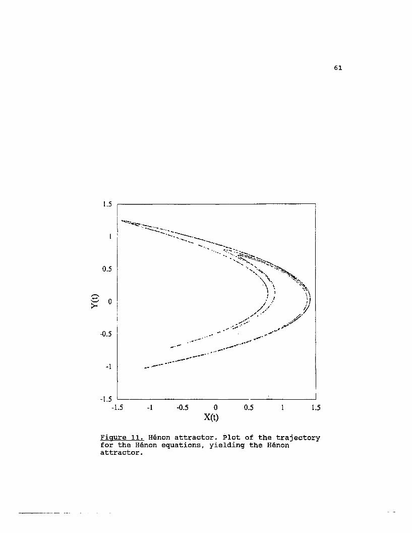
1.5

0.5

.-、

ξ o

-0.5

“;안:““‘.“"‘

‘-~닫'.‘‘--“·“--...-

“ ‘ :‘ ~““".환등5 ‘

".、，、;;윗?\

‘、센‘·꽃상­‘ -.

i X 원‘i ; 1\

/ :' !J/./ if

//. -- ‘~.’• 1'/

",- -,y'

.,.<-..'" _<.J':"01" .~ ........ ' __, ...,,-

.#

”-", -""'-.,.-- __ tII'- •

...’ ..-"-_..----'_....-_ •...,..,. ... -

_.~ ..--

61

-1.5-1.5 -0.5 O

X(t)0.5 1.5

Fiaure 11. H흔non attractor. Plot of the trajectoryfor the Hξnon equations , yielding the Henonattractor.

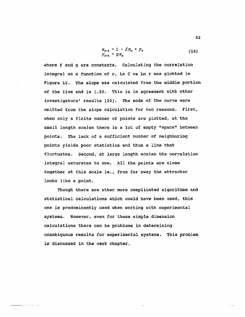
X n+1 = 1 - fXn + YnYn+1 = gXn

62

(16)

where f and g are constants. Calculating the correlation

integral as a function of r , Ln C vs Ln r was plotted in

Figure 12. The slope was calculated from the middle portion

。f the line and is 1.26. This is in agreement with other

investigators' results [20]. The ends of the curve were

。mitted from the slope calculation for two reasons. First ,

when only a finite number of points are plotted , at the

small length scales there is a lot of empty "space" between

points. The lack of a sufficient number of neighboring

points yields poor statistics and thus a line that

fluctuates. Second , at large length scales the correlation

integral saturates to one. All the points are close

together at this scale ie. , from far away the attractor

looks like a point.

Though there are other more complicated algorithms and

statistical calculations which could have been used , this

。ne is predominantly used when working with experimental

systems. However , even for these simple dimension

calculations there can be problems in determining

unambiguous results for experimental systems. This problem

is discussed in the next chapter.

63

7/

//

/

//

//

//

/

/

/

q

’

/

/

따Be14

M

빼curve

9

Fiaure 12. Ln of Correlation Length vs.size for the Henon attractor. This is an。f how the slope of this plot yields thecorrelation dimension. The upper line is forreference and has a slope of 1.26. The loweris from the Hξnon data.

CHAPTER VII

IMPLEMENTATION OF CONCEPTS IN AN EXPERIMENTAL SITUATION

The previous chapter introduced some of the concepts

necessary to understand or describe properties of dynamical

systems. But in all the examples , the equations that

governed the dynamics were given explicitly. However , the

experimental scientist does not typically have the equations

。f state at hand and might only have an imprecise knowledge

。f the relevant physical variables. (This discussion is

based on the tacit assumption held by most scientists that

there is some underlying set of deterministic equations

governing the physical processes. Whether they are known or

not is another question.) Furthermore , when one performs an

experiment usually only one or two of the relevant physical

variables are probed or sampled. The difficulty arises in

。btaining phase plots of some natural phenomena when only

incomplete information exists. There is a remarkable

theorem by Dutch mathematician F. Takens that makes possible

the connection between actual experiments and numerical

experiments and mathematical analysis. This theorem says

that one can still reconstruct a phase plot that in some way

resembles the "true" phase plot by only having knowledge of

。ne of the systems' variables [32]. By resemblance , it is

65

meant that the phase plots share some of the same

geometrical or topological features , such as dimension. At

first , this conjecture seems false: How can the dynamics of

a multidimensional system be reconstructed from only one

component. However , if these sets of equations governing

the systems dynamics are coupled to each other , (see

Equation. 16 , the Hξnon equations.) then one variable

contains information about the other variables. The

experimenter has to insure that the variable observed is one

that is coupled strongly to the system of interest.

This "reconstructed ll plot can be created by various

techniques , but the one usually chosen by researchers is

time series reconstruction by the method of delays [33].

other methods involve taking multiple derivatives or

integrals of the time series and using them to create the

additional lI independent" axes. However , taking higher

derivatives of discreetly sampled data can cause problems as

the results will appear to change more abruptly than in the

continuous physical case. To perform a time series

reconstruction by the method of delays , one first takes a

sequence of data from one of the physically relevant

variables at equally spaced time intervals ie. a time

series. This discretization process from the continuous

variable can be represented as:

66

X t l

X(t) .. (17)

x

where t n represents the time at which the nth data point is

。btained. One then plots this series vs. itself , but at a

later point ~ , in time. (See Figure 13 for a pictorial

representation in 2 dimensions). This can be generalized t。

an m-dimensional vector by use of increasing time delays as

follows:

효 (ti ) = [X( tJ ' x( t i +-;) , X( ti + 2τ ) , … x(ti +(m-l)-;)] (18)

In this way , a 1-dimensional scalar is embedded into an m­

dimensional vector space. Since one does not usually know

the dimension of the system under study , these "embedding"

dimensions can be made increasingly larger until they exceed

the true dimension of the attractor. This way , if the

。bject (the reconstructed attractor) embedded has in reality

a dimension less than the embedding dimension then , the

calculated dimension will , too. An example of this is a

line which still has a dimension of one whether it is drawn

。n a two-dimensional plane or in a three-dimensional volume.

The only restriction of this embedding technique is that for

some objects the embedding dimension used must be greater

than (2d + 1) , where d is the attractor's true dimension

[34]. Conversely , if the attractor's true dimension is

greater than the embedding dimension then the calculated

67

dimension will yield the value of the embedding dimension.

Although this procedure is easy to implement , when

working with a real data set which is limited in size and

precision , the results can be less than conclusive. The

reason is that Takens' theorem guarantees that the true and

the reconstructed attractor are similar for a system in

which an infinite amount of noise free data can be analyzed.

It is unclear how well the reconstructed attractor converges

towards the true one , for a noisy and finite set of data.

Indeed , many experimenters have discovered how "good" the

reconstruction is depends on the time delay chosen , noise

level , and the total number of points evaluated [35 ,30].

Unfortunately , this problem is not resolved and to make

things worse it is generally not possible to differentiate

between systems a priori that are sensitive to the

reconstruction parameters and the data and those that are

not. What one does is analyze the data in a number of

different ways , applying other researchers empirical

findings as to which delays work best. Some of these

findings by other researchers will briefly be discussed.

The first technique is to plot the autocorrelation

function as a function of the time delay and find the first

minimum. This function is defined as:

H( 't)=잖 E;=1 Xi *Xi+'f (19)

This value of the time delay is then used in the phase space

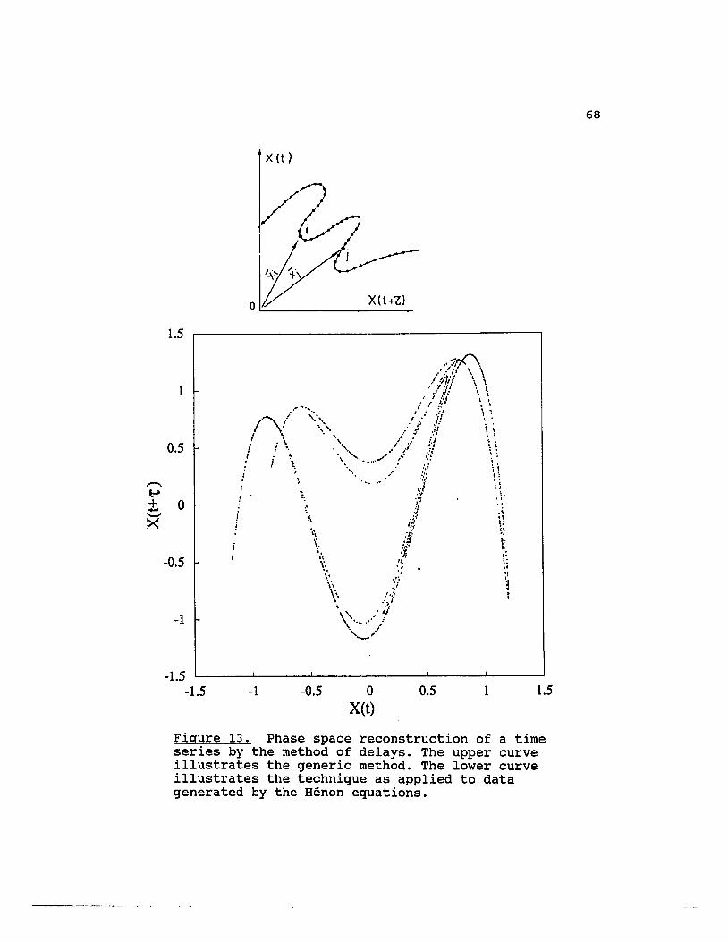
68

X(t )

X(t+'l)

;;j;·

,‘....‘---”’

”·j이U

안h‘‘;•.,-

lll

j··‘‘

!‘1,‘‘..‘-

-‘、‘

ι까사’’;.，

·/‘,.----젠씌·파?’

’

---/

.,

--·it--”‘.

·IL-----”··‘

·r·꾀씌‘，끼싸」

μ··‘;

•

/

,J

·j‘w”

----μJlc;.시-갚센낸!，

•..i

tι

•

t··7·

”---

/.

”

;,/

/닌)

、

.、

---\‘、.、

、、‘‘

、

·‘

‘.!

‘.””‘‘‘··r‘.

‘、‘얀·‘

L·시”·‘.

‘、、.

‘.j”·jv‘--

,...,

‘.t-,

,

.

---‘,~、‘，‘

·t’·l

//

jl

---

1.5

0.5

0

-0.5

(e+})씨

1.50.5X(t)

-0.5-1.5

-1.5

Fiqure 13. Phase space reconstruction of a timeseries by the method of delays. The upper curveillustrates the generic method. The lower curveillustrates the technique as applied to datagenerated by the H응non equations.

69

reconstruction. If the time delays are too short (short is

a relative term and depends on the behavior of the system

under study) , then the signal looks too much like itself

(ie. nothing has changed). A phase plot in two dimensions

would just be a diagonal line of y = x. If the delay is to。

long and the signal is chaotic , this indicates the signal at

a later time will have no correlation with itself at earlier

times (ie. all predictability is lost). A two dimensional

plot of this would look like a random scatter of data. By

locating the first minimum of the autocorrelation function ,。ne evaluates the data at time scales in between these tw。

extremes.

The other technique is to find the minimum of the

mutual information function defined by Fraser [36]. For

some systems this resulted in a better reconstruction than

when the autocorrelation was used. The problem with using

the mutual information is that it is rather cumbersome t。

implement. other researchers have shown that plotting the

correlation integral as a function of delay (keeping r

fixed) and noting the first minimum , the same as the mutual

information function [37].

Another concern when performing .real or numerical

experiments is the introduction of noise into the system.

For numerical experiments the "noise" is a result of

truncation and roundoff by the computer [35 , 38]. Noise

does not appear to be a major problem, but it would be

70

prudent to keep it as small as possible. Noise blurs the

transition between different modes of behavior (ie. regular

。r chaotic) and the patterns in the phase plots fill out ,thus obscuring any fine structure to the attractor [39].

This filling out process makes the underlying attractor

appear to be higher dimensional than it really is. This is

so because noise is "space filling" , and by definition , has

as infinite number of degrees of freedom , and thus

dimensions.

The last significant problem to be addressed concerns

real data sets and state space reconstruction is - how many

data points are required to get a good reconstruction?

This , like many of the other problems discussed , does not

have a definitive answer and may depend on the specific

system under study. Many authors have "derived" the minimum

required data points for an accurate reconstruction [40 ,41].

The exact numbers and exponents may vary , but the required

number of points N iS , thought to have an exponential

dependence on the "true" dimension of the system. The

estimates given range from N-10d/2 to N-42d, where d is the

attractor dimension. For example in six dimensions (which

is not unreasonable for some physical systems) this

translates to a minimum of 1000 points or a maximum of 5

billion. As one can see this is a large discrepancy and it

is not possible a priori to decide which estimate to use.

One empirical method to help decide this question is t。

71

repeat the calculations with an increasing number of points

and see if the results converge. The number of data

required is an important practical question because some of

the algorithms require iterations that scale with the square

。f N. If N is too large it takes a prohibitively long time

to make the calculations.

As suggested , analysis of experimental data from some

。f the techniques previously mentioned can be problematic.

The results can be inconclusive particularly when answers

are sought to the absolute value of the dimension of the

attractor. However , if one is only looking for relative

changes in these quantities as a function of the system's

parameters , then their utility is probably enhanced. In

effect , the resultant calculations for a physical system

would provide a "signature" for the ongoing processes , much

like spectral analysis provides for linear systems. It is

from this perspective of relative changes that my heat

transfer data has been analyzed. It is hoped that this will

provide a characterization of the approach from nucleate

boiling to film boiling.

CHAPTER VIII

DYNAMICAL SYSTEMS RESULTS

A summary of the experimental configuration used for

collecting the temperature and heat flux data is given.

However , a more detailed discussion of the apparatus is

found in Chapter III , because it is essentially the same set

up as for Part I of this research.

A platinum wire of 0.1 mm diameter and 1 cm effective

length was placed vertically inside the center of a double

glass dewar , both of which were filled with LN2. The inner

dewar is 5 cm in diameter and 1 m in length. An adjustable

constant current source was connected to the platinum wire

to provide heating. After low pass filtering at a cutoff

frequency of 1 kHz (this frequency was determined from

measurements of the temperature spectrum and aliasing

considerations) , the temperature signal from the wire was

recorded for various steady increasing currents until film

boiling commences. The fluctuating temperature data that

were then analyzed. The maximum fluctuation was 0.5 kelvin ,but the temperature resolution of the thermometer is a few

millikelvins.

73

FOURIER TRANSFORM RESULTS

The plots in Figure 14 are the amplitude of the Fourier

transform of the temperature fluctuations. The three plots

correspond to progressively increasing currents. The

spectrum has a 11f shape and as the current increases the

curve expands outward to include higher frequencies. Note

this was not a spurious signal due to 11f noise commonly

found in electronics , as evaluation of the background noise

showed it to be a few hundred times smaller than the

temperature signal. However , there did not appear to be any

discernable characteristic frequencies for these three plots

。r any of the other data sets evaluated. This may not be

informative as a chaotic signal may posses a few periodic

components in addition to the required broadband spectrum.

One form of chaos signified by the intermittency route t。

chaos exhibits a 11f spectrum [42 ,43].

The heat flux was calculated from the temperature data

as was done in Part I of this research (see Equation 6) and

its spectrum is plotted in Figure 15. Again , a similar but

not identical , 11f pattern emerges. There was also a hump

in the spectrum which moves outwards when the average power

was increased. However , there did not appear to be any

quantitative trend in either the amplitudes or frequencies

。f the heat flux spectrum as a function of heater power.

The temperature and heat flux are some of the dominant

variables that characterize this system. Apparently , the

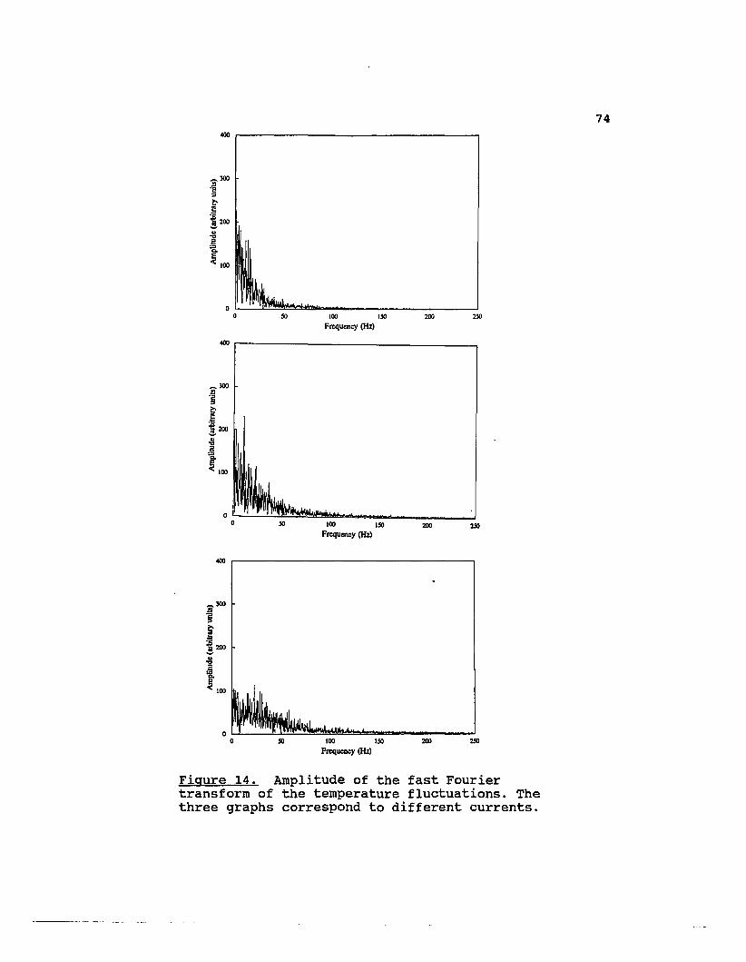
‘m

툴펼 200

혈

훌 100

g 200 2!0100 150

Frequency (Hz)

‘m

뼈

m

m

(김taaaa퍼염)USE료를〈

g 100 150

FrequCllcy (H찌

X찌 2!0

«xl

뼈

뼈

뼈

(g·si감”g힐염)”gE품E〈

50 100 150

Frequency (Hz)2!0200

Fiaure 14. Amplitude of the fast Fouriertransform of the temperature fluctuations. Thethree graphs correspond to different currents.

74

100

@

%

찌

(S걷그간ag퍼a)ugg넘Rξ〈

20

% \00 150

Fπquency (Hz)200 250

100

@

“w

때

(S·ai

늙ig·￡a)”sE료E〈

g

SO 100 ISO

Frequency (Hz)200 %so

100

@

mw

찌

(g걷aaig펀‘)uSE료를〈

20

oo 100 ISO

Frequency (Hz)200g

Fiaure 15. Amplitude of the Fast Fouriertransform of the heat flux fluctuations. The threedifferent curves correspond to different currents.

75

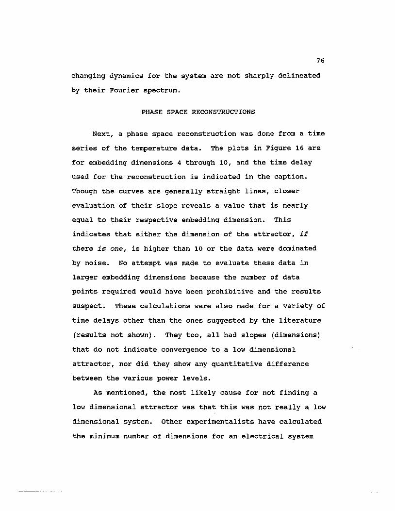
76

changing dynamics for the system are not sharply delineated

by their Fourier spectrum.

PHASE SPACE RECONSTRUCTIONS

Next , a phase space reconstruction was done from a time

series of the temperature data. The plots in Figure 16 are

for embedding dimensions 4 through 10 , and the time delay

used for the reconstruction is indicated in the caption.

Though the curves are generally straight lines , closer

evaluation of their slope reveals a value that is nearly

equal to their respective embedding dimension. This

indicates that either the dimension of the attractor , if

there is one , is higher than 10 or the data were dominated

by noise. No attempt was made to evaluate these data in

larger embedding dimensions because the number of data

points required would have been prohibitive and the results

suspect. These calculations were also made for a variety of

time delays other than the ones suggested by the literature

(results not shown). They too , all had slopes (dimensions)

that do not indicate convergence to a low dimensional

attractor , nor did they show any quantitative difference

between the various power levels.

As mentioned , the most likely cause for not finding a

low dimensional attractor was that this was not really a low

dimensional system. other experimentalists have calculated

the minimum number of dimensions for an electrical system

77

。

o

?

/"/-"--

。

’/,J’’/

//-

,II/­--/

익

。

q

vs. ln of boxdata. Thedifferent

q

Fiqure 16. Ln of correlation lengthsize for the temperature fluctuationthree different curves correspond t。

currents.

。

。

78

that exhibits a l/f spectrum to be more than 20 [43]. For

the boiling heat transfer system, it was reasonable t。

assume the smallest unit or component comprising it is a

single nucleation site. This bubble site contributed a

minimum of one degree of freedom. From visual observation

。f the heater , the diameter of the bubbles at departure were

0.2 mm and the effective size of the heater/thermometer was

10 mm. Thus , depending on the heat flux , tens or hundreds

of bubbles may have been originating on the wire. If these

bubble sites were not strongly coupled to each other , then

the effective number of degrees freedom was just the total

number of bubbles , thereby precluding any low dimensional

dynamics. It is not feasible to monitor a smaller boiling

patch with the platinum wire for two reasons. First , the

sensitivity of the thermometer decreases linearly with the

length of the heater and would lead to a.resolution that is

too coarse. Second , end effects due to the current and

voltage leads would interfere with the heating , boiling , and

measurement processes.

There are additional experimental limitations that

could have a detrimental effect. The dynamic range of the

measurements was less than 55 dB because of noise. It is

not clear how much this noise could be reduced. Also , a

counter intuitive effect was that low pass filtering the

signal could increase the dimension of a chaotic signal

[44]. It was not clear what the optimal sampling rate , or

79

duration is for this system. If one were just interested in

the temperature measurements , then sampling sUfficiently

above the highest signal frequency , mi당ht have been a good

estimate. However , one is also interested in taking

derivatives of the signal for plotting in phase space and

this would increases the sampling requirements. Due to the

AID data acquisition system there was a limit to the number

。f points that can be recorded. Grossly oversampling t。

achieve smoother derivatives is not a viable option because

。f memory limitations of the computer. It did not appear

that these problems could readily be solved; therefore an

additional set of experiments with slightly different goals

was performed. However , this will be presented the

Appendix.

FLUCTUATIONS IN THE Q - T PLANE

As mentioned, the heat flux and temperature are some of

the important parameters characterizing the system. While

the tiπe dependence of these quantities appear to behave

randomly , maybe there is a strong correlation between these

two variables. Plotting the trajectory of Q and T(t) could

reveal some of their underlying dynamics. F’igure 17 shows a

sequence of plots for increasing power levels. The

horizontal (temperature) axis range is 1 kelvin wide and the

vertical (heat flux) axis range is 1 w/cm2 • The offset is

adjusted so that Q and T are both centered on their

80

respective average values (not given). This indicates much

more of a pattern than the previous results. It was

difficult to tell from the static figure , but by observing

the computer slowly plot the trajectory , the trace could be

seen to be a crude ellipse which on average follows a

counterclockwise trajectory about some average heat

flux 00 1 and average temperature To. The fact that this

trajectory did not just show random fluctuations , was at

first striking , and unexpected. This pattern seems t。

indicates an underlying dynamic. Therefore an attempt was

made to construct a qualitative physical picture or model

that is consistent with this motion. Also , an analysis of

the relevant equations were made to see if they predict this

motion.

Figure 18 shows a hypothetical trajectory in

the Q-T plane along with a portion of the characteristic

nucleate boiling curve superimposed. (The argument is

qualitative so the actual units used and the exact shape of

the curve were not calculated explicitly.) Also shown are

the lines of constant average heat flux 00 and constant

average temperature To. These lines intersect on the

boiling curve. The sequence of points A through 0 represent

the "life cycle" of a nucleation site on the heated surface ,thus this was from a localized or microscopic point of view.

At point "A" a bubble starts to form in the superheated

liquid as power is continually dissipated into the wire.

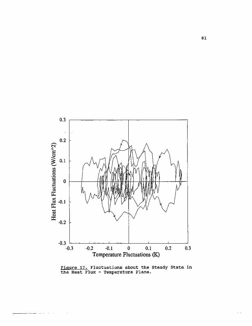
0.3

0.2

r ‘<

EU

둠 0.1

CI)특。

헐 o~uzμ닉

설 -0.1P~

cdQ)

빌-0.2

-0.3-0.3 -0.2 -0.1 0 0.1 0.2

Temperature Fluctuations (K)0.3

81

Fiaure 17. Fluctuations about the Steady state inthe Heat Flux - Temperature Plane.

82

This absorbs some of the heat but does so isothermally

(step A-B). When the bubble increases in size it begins t。

insulate the wire , thus diminishing cooling by mean를 。f

conduction or convection and driving up the temperature

(step B-C). Finally , the bubble becomes large enough that

it breaks off and leaves the surface because of buoyant

forces. The cold liquid then rushes in, thereby increasing

the heat flux and decreasing the temperature (C-B-A). The

process repeats itself as a new bubble starts to form.

While this last scenario is reasonable , it seems t。

predict that counterclockwise motion is the only one

allowed. Observation of the experimental data indicate that

while on average this is true , it is not rigorously true for

every successive point. So , how does this apparent

violation come about? The problem lies in the boiling curve

drawn in the Q-T plane. Typically , this empirically

derived curve can be approximated by an equation which has

the form:

Q = h J1 T" { 1sαs3} (20)

where h is the heat transfer coefficient. This curve is not

really a sharp line which remains stationary in time; it is

an average. More appropriately , it can be thought of as a

family of similar , closely spaced curves. The overall

instantaneous state of the system determines which curve the

system is on. That is , although the temperature and heat

flux are the dominant variables in determining these boiling

헬 ioQ

섭각

83

6. ToSuperheat temperature

Fiqure 18. Life Cycle of a Bubble in the HeatFlux - Temperature Plane.

84

curves , there are other less important degrees of freedom as

well. For example , how many bubbles surrounded the surface ,。r what was the local convective flow pattern? The true

trajectory followed a unique path in some higher dimensional

phase space which included all the relevant variables. A

particular boiling curve was realized by "slicing" this

higher dimensional manifold to the Q-T plane. Different

parallel "slices" correspond to different external

conditions in the system or equivalently , to different

times. In effect the system ’'sees" a time varying heat

transfer coefficient.

Another , more analytical way to show this uses the

conservation of energy concept. Referring to Figure 18

again , the Q-T plane can bε divided up into 4 quadrants.

The constant Qo line and the boiling curve were the dividing

lines. Energy conservation requires that the power input t。

the heater must show up as either heat flux Q, out through

the surface or , because of the nonzero heat capacity of the

heater , as an increase in the temperature T of the heater.

Mathematically this is stated (see Equation 6 for

explanation of terms):

Given that the applied power is constant , the long time

averaged steady state heat flux Q is:

(6)

85

Q=p= 00 (21)

where 00 is the steady state heat flux. The steady state

temperature is denoted by ATo• One is interested in the

variables Q and AT and their fluctuations about their

steady state values. These variable are defined as:

5AT=AT-A낌

5AO = 0 - 0，。(22 )

The time derivatives of these variables were examined t。

ascertain whether restrictions apply to their sign.

Rewriting Equation 6 in terms of 8AT and 80 gives:

쁘으! = 혹 (On - 0) = -추 50dt C ·-u

This yields

d8AT _ J < 0 when 0 > 00 = p감t - ) > 0 when 0 < 00 = p

(23 )

(24 )

Therefore , the line 00 is the dividing line which determines

d5A ’I ’the sign of ~믿:~. The position in phase space relative t。

the steady state heat flux curve helped determines the sign

。f 브앨 , but not in all four quadrants. In essence , thedt

trajectory "wants" to return to the equilibrium heat flux

curve. This allowed a trajectory in the first and third

d5Qquadrant to have either a positive or negative ~:~~. Itdt

will have to be determined by more sophisticated analyses

and experimentation whether there is a physical preference.

Because of conservation of energy , quadrants two and four

d56require that ~;~~ be negative and positive respectively.dt

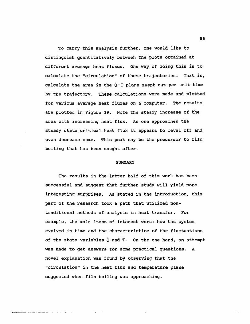
86

To carry this analysis further , one would like t。

distinguish quantitatively between the plots obtained at

different average heat fluxes. One way of doing this is t。

calculate the "circulation" of these trajectories. That is ,

calculate the area in the Q-T plane swept out per unit time

by the trajectory. These calculations were made and plotted

for various average heat fluxes on a computer. The results

are plotted in Figure 19. Note the steady increase of the

area with increasing heat flux. As one approaches the

steady state critical heat flux it appears to level off and

even decrease some. This peak may be the precursor to film

boiling that has been sought after.

SUMMARY

The results in the latter half of this work has been

successful and suggest that further study will yield more

interesting surprises. As stated in the introduction , this

part of the research took a path that utilized non­

traditional methods of analysis in heat transfer. For

example , the main items of interest were: how the system

evolved in time and the characteristics of the fluctuations

。f the state variables Q and T. On the one hand , an attempt

was made to get answers for some practical questions. A

novel explanation was found by observing that the

"circulation" in the heat flux and temperature plane

suggested when film boiling was approaching.

7

깐、(gi다그 5

끔)여-iA-끽φ{늘

쇠킬되 ’j

」Ug

〈여~ 2‘

1

,//0

0 2 4 6 8 10Power (W/cm ‘ 2)

Fiaure 19. Area per unit Time Swept out in theHeat Flux - Temperature Plane.

87

88

。n the other hand , some of the other analyses gave

inconclusive results. But the structure observed in the Q-T

plane is suggestive that more sophisticated experimental and

analytical investigations may lead to an unequivocal

determination that chaos is present. Also , this research

produced some interesting and unanswered physics questions

concerning the nature of nucleation. Analogous to the

Faucet Drip Experiment , can single nucleation sites exhibit

chaotic rhythms? (See Appendix) and " Do aggregates of these

sites behave in some sort of collective manner which can be

described by simple , low dimensional dynamics?" I hope

that sufficient curiosity has been aroused , and the

groundwork laid to insure that this line of research will be

continued.

CHAPTER IX

CONCLUSIONS

This work was divided into two parts. The first part

dealt with measurements of temperature and heat flux under

conditions of steady state and transient heating. It was

found that transient heating caused a 30옹 reduction in the

critical heat flux compared to that of the steady state

values. The reasons for this reduction was suggested to be

the lack of well developed convection currents in the

liquid. Consequently , forced convection was investigated t。

eliminate the premature transition to film boiling. The

data indicated that flow rates of less than one meter per

second were successful in suppressing the premature

transition to film boiling. This was quite a significant

increase (more than 300옹 in some cases) in critical heat

flux.

Also , noting that slightly different heater and dewar

configurations sometimes gave significantly different

results , investigations were made to characterize these

different parameters. It was determined that the heat leak

into the dewar and a confining geometry contributed to the

variations in the critical heat flux. The reason boiling

heat transfer in a confined geometry reduced the overall

90

effects of any natural convection was that the resultant

bubbles could not disperse as easily.

The second part of the analyses was from a dynamical

systems point of view in which the time evolution of the

heat transfer system was of primary concern. Here steady

state measurements yielded data which were not so steady

afterall , were analyzed. This work consisted of examining

the evolution (in time) of the fluctuating system

variables Q and T to see whether any insight or predictive

information could be gained. Some aspects of this analysis

worked better than others , but with experimental and

analytical refinements , improvement seems possible. For

example , by observing that the "circulation" of the heat

flux and temperature reaches a peak as the transition t。

film boiling was approached , a possible precursor to film

boiling was discovered. The other analyses such as the

Fourier spectrum or correlation dimension calculations gave

inconclusive results. On the other hand , this research

produced some interesting and unanswered physics questions

concerning the nature of nucleation. "Can single nucleation

sites behave in a chaotic matter? " and " Do aggregates of

these sites behave in some sort of collective manner which

can be described by simple , low dimensional dynamics? "

Overall , these results have added significant new data

to the heat transfer literature , and indicate that

previously neglected questions in heat transfer are

91

important after all. This study also generated some

interesting insights and novel analyses for a very

traditional sUbject. Hopefully , this course of inquiry will

encourage new research or a continuation of this work.

REFERENCES

1. P. Komarek , The implications of higher criticaltemperature superconductive materials , in proceedings ofthe twelfth Int. Cryogenic Engineering ConferenceButterworth , Guildford , U.K. (1988) p. 64.

2. R. K. Kirschman , Cold electronics: an overview, Crvoqenics(25) 115 (1985).

3. G.M. chrysler , and R.C. Chu , cooling of high powerdensity electronic chips , in: Advances in cryogenicEngineering , vol. 35 , Plenum Press , New York (1990).

4. W. Frost (ed.) , Heat Transfer at Low Temperatures , PlenumPress (1975).

5. Y.S. Touloukian et aI , Thermal Diffusivity , Vol. 10 ofThermophysical Properties of Matter. Plenum Press , NewYork (1973).

6. D.N. Sinha et aI , Premature transition to stable filmboiling initiated by power transients in liquid nitrogen ,Crvoqenics 19(4):225 (1979).

7. Eric W. Roth , Erik Bodegom , L.C. Brodie , and J .S. Semura ,in: Advances in Cryogenic Engineering , Vol. 35A, PlenumPress , New York (1989) , p. 447.

8. P. J. Giarratano , Transient boiling heat transfer from tw。

different heat sources: small diameter wire and thin filmflat surface on a quartz sUbstrate , Int. J. Heat MassTransfer 27(8):1311 (1984).

9. A.C Rose-Innes , and E.H.Roderick , Introduction toSuperconductivity , 2nd ed. Pergamon Press (1978).

10. P.G. Koskey and D.N. Lyon , Pool boiling heat transfer t。

cryogenic liquids , AIChe Journal; May , 1968 p. 372.

11. J .R. Holman , Heat transfer , 5th ed. McGraw-Hill , NewYork (1981).

12. M. Blander and J.L. Katz , Bubble Nucleation in Liquids ,AIChe Journal; September , 1975 p. 833.

93

13. W.M. Rohsenow (ed.) , Handbook of Heat Transfer 3rd ed.McGraw-Hill , New York (1973).

14. V. P. Skripov, Metastable liquids , Wiley , New York ,(1974).

15. D.N. Sinha , L.C. Brodie , and J.S. Semura , Liquid-to-VaporHomogeneous Nucleation in Liquid Nitrogen , Phvs. Rev.B36 (7) : 4082 (1987).

16. P.G. Knibbe , The End-Effect Error in the Determination ofThermal Conductivity Using a Hot Wire Apparatus , Int. J.Heat Mass Transfer. Vol 29 , No.3 , p.463 (1986).

17. B. HaOkansson , P. Andersson , and G. B!ckstr6m, ImprovedHot-wire Procedure for Thermophysical Measurements underPressure , Rev. Sc. Instrum. 59:2269 (1988).

18. L.A. Hall , Survey of Electrical Resistivity Measurements。n 16 Pure Metals in the Temperature Range 0 to 273 K.NBS Tech. Note 365-1. National Bureau of standards ,Boulder , Colorado (1968).

19. H.S. Carslaw , J.C. Jaeger , Conduction of Heat Solids2nd ed. , Oxford University , London (1959) p.344.

20. O. Tsukamoto , T. Uyemura , and T. Uyemura , Observation ofbubble formation mechanism of liquid nitrogen subjectedto transient heating , in: Advances in CryogenicEngineering , Vol. 25 , Plenum Press , New York (1980) ,p.476.

21. J.S. Trefil , Introduction to the Physics of Fluids andSolids , Pergamon Press , New York (1975).

22. Roderick Jensen , Classical chaos , American Scientist vol.75 March-April (1987) p. 168.

23. E.A. Jackson , Perspectives of Nonlinear Dynamics , Vol.1 ,Cambridge University Press (1989).

24. E. N. Lorenz , Deterministic nonperiodic flow , J. Atmos. Scivol. 20 p.130 (1963).

25. H.L. Swinney and J.P.Gollub , The transition t。

turbulence , Phvsics Todav 31(8) ,41 (1978).

26. P. Bergξ， Y. Pomeau , and C Vidal , Order within Chaos ,John Wiley and Sons (1984).

27. L. E. Reichel , A modern course in statistical physics ,University of Texas Press , Austin (1980).

94

28. Peter Grassberger and Itamar Procaccia , Measuring thestrangeness of strange attractors , Phvsica 9D (1983)p.189.

29. B.B. Mandelbrot , The fractal geometry of nature ,W.H.Freeman (1983).

30. N. Gershenfeld , in: Directions in Chaos , vol. 2 , ed. B.I.Hao , World Scientific Press , (1988)

31. M. Hεnon ， Numerical study of quadratic area-preservingmappings , Ouart. of ADDI. Math 27 , p. 291 (1969).

32. F. Takens , Detecting strange attractors in turbulence ,in: Dynamical Systems and Turbulence, Warwick 1980Lecture Notes in Mathematics 898 , ed. D.A. Rand and L.S.Young , Springer-Verlag.

33. N.H. Packard et aI , Geometry from a time series , 요뇨X흐:

Rev. Letters 45 , p. 712 (1980).

34. H.Whitney , Differentiable manifolds , Ann. Math. 37 ,p.645 (1936).

35. M. Casdagli , State space reconstruction in the presence。f noise , Phvsica D 51 (1991) p. 52.

36. A.M. Fraser and H.L. Swinney , Independent coordinates forstrange attractors from mutual information Phvs. Rev. Avol. 33 , (1986) p. 1134.

37. W. Liebert and H.G. Schuster , Proper choice of the timedelay for the analysis of chaotic time series , ~뇨X르

Letters A, vol. 142 number 2 ,3 (1989) p. 107.

38. G.A. Bennetin , On the reliability of numerical studies ofstochasticity, Nuovo Cimento 44B (1978) p. 183.

39. A. Ben-Mizrachi and I. Procaccia , Characterization ofexperimental (noisy) strange attractors , Phvs. Rev. Avol. 29 , (1984) p. 975.

40. L. Smith , Phvs Letters A, vol. 133 (1988) p. 283.

41. J.P. Eckmann and D. Ruelle , Fundamental limitations forestimating dimensions and Lyapunov exponents in dynamicalsystems , Phvsica 0 56 (1992) p. 185.

42. H.G. Schuster , Deterministic chaos: an introduction , 2nded. , VCH , Cambridge (1988).

95

43. N.A. Gershenfeld , Dimension measurement on high­dimensional systems Phvsica D 55 (1992) p. 135.

44. R. Badi et aI , Dimension increase in filtered chaoticsignals Phvs. Rev. Letters 60 , p. 979 (1988).

45. R.Shaw , The dripping faucet as a model chaotic system ,Aerial Press , Santa Cruz , CA (1984) p. 368.

46. R.F. Cahalan et aI , Chaotic Rhythms of a dripping faucet ,Computers in Physics , Jul/Aug (1990).

APPENDIX

BUBBLE DROP EXPERIMENT

In view of the problems mentioned in Chapter VIII , an

alternative and simplified experiment was to observe what

。ccurs at just one bubble site. However , this is not really

the same problem as discussed previously because the system

has been simplified too much. Having one isolated bubble

site means there is not any interaction with other bubble

sites. The most that could be learned concerns the dynamics

。f a single nucleation site. The process of pool boiling

developing into film boiling is a collective phenomenon , and

this collective process was the desired observable.

Nonetheless , characterizing the fundamental component of the

system, the nucleation site , is an important step t。

understanding the boiling process as a whole. Therefore an

experiment was devised in an analogous fashion to Shaw's

。ften studied chaotic water drop experiment [45 ,46]. In

Shaw's experiment the time between drops originating from a

dripping water faucet was observed. At low average drop

rates the drops detach periodically , but with increasing

drop rates there was more than one period , and finally the

drop rates appear to vary chaotically from drop to drop.

In the single bubble site experiment , bubbles from one

97

nucleation site were created and observed , to obtain

quantitative values for bubble velocity and departure rates.

The analysis is similar to Shaw's in that the various

periodicities of the bubble departure rates were the main

。bservable.

Because of the limitations of the heater/thermometer

previously discussed , a new apparatus was designed that

gives information other than temperature and heat flux. The

variables that could then be observed were the bubble

diameter , velocity and departure rate. It was not possible

to measure the temperature , and the heat flux was only known

。n a relative scale. The single bubble generator was

fabricated as follows (see Figure 20). A cylinder 3.5 cm in

diameter and 2 cm long was constructed out of an insulating

material (TEFLON). Towards the top inside portion of the

cylinder was placed a small diameter (0.4 cm) metal rod

wrapped with thin gauge wire in which current was passed t。

provide Joule heating. An additional vertical hole (0.6 mm

dia.) was made through the top of a cover plate down to the

heater. This cover plate could be interchanged so that

different size cavities could be tested. This cavity was

the artificial nucleation site and produces bubbles

nominally 1.2 mm in diameter when heat was dissipated in the

wire. Note this size was considerably larger than the 0.2

mm bubbles seen originating from the platinum wire and

corresponds to a vapor volume over 200 times larger.

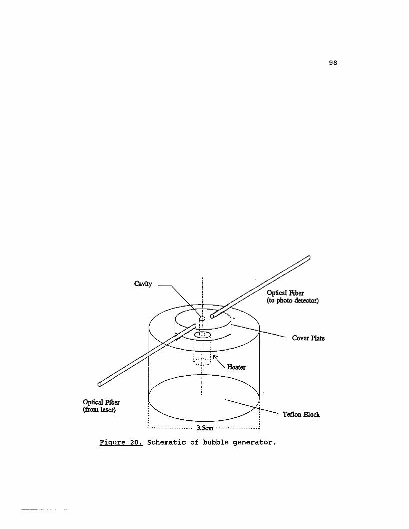
Optil앓I Fib많

(from 뼈ser)

Cavity

;\~-- ---〉석

Cover Plate

Teflon Block

98

Fiaure 20. Schematic of bubble generator.

99

However , this was intentional because of the limited

sensitivity of the bubble detection apparatus.

Bubble detection was achieved by optical measurements.

Light from a helium-neon laser was routed through a plastic

。ptical fiber (1.4 mm dia. core) into the dewar and aligned

adjacent to the nucleation site. Directly opposite this was

another fiber which receives the laser light and transmits

it to a photodiode/amplifier assembly outside the dewar.

When the bubble passes between the fibers it scatters the

incoming laser light , thus reducing the light detected by

the photodiode. The scattering effect was not large and was

the reason that very small bubbles , though visible to the

eye , could not be detected by the electronics. The

photodiode and amplifier assembly have a response time

shorter than 10 μ S , more than adequate for observing the

bubbles which had departure times greater than 10 ms. After

low pass filtering the amplified photodiode output , the

analog voltage signal was digitized at a rate of 10 ,000 per

second and stored in the computer. The bubble diameter and

velocity were measured from recordings made with a home

video camera; however , resolution was limited due t。

performance limitations of the camera. Some of the

conclusions reached are as follows. The bubble reached

terminal velocity of 100 em/sec 20 ms after release from the

artificial nucleation site.

The primary analysis consisted of calculating the

100

elapsed time between bubble departures. A computer program

was written such that the positions (in the time series) of

the local minima in the photodiode signal level was

recorded. These minima corresponded to bubbles passing

through the detector and blocking the light received by the

photodiode. These bubble departure times were then plotted

vs. the bubble number to see whether any patterns emerge.

The sequence of graphs in Figure 21 are from low heater

currents to high ones. As can be seen from the top plot

there is a characteristic time between bubbles of 310 ms

There was also a second characteristic time of 760 ms that

。ccurs after the passage of approximately 20 bubbles.

similar interesting patterns can be seen from the other tw。

plots. Upon reflection , this was an unexpected result.

Typically , one would expect some mean bubble departure time

that had a normally distributed uncertainty. In fact , these

patterns are reminiscent of those seen in Shaw's water drop

experiment before chaos had set in. However , the results

are problematic in that the reproducibility is poor. Even

though many of the data sets show two or more characteristic

times in a very regular fashion , if one attempts to repeat a

run under the exact experimental conditions , different

results could be obtained. For example , the apparatus could

be removed from the dewar , warmed to room temperature , and

then reinserted into the LN2. The new data set could yield

different results than the previous set. Also , the device

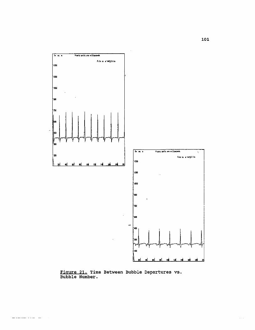
Tn US n Y·.I.udl‘ ·π .ill......

r,lt I‘ •빼』 “”IJ밍

1200.

1050

!OJ

m

lilIl

뼈

Dl

l잊

2111 411 601 삐 삐 삐 I" 1&4 I메 a

101

Tn VI n

fllf I“ 、.4.1‘ lift

’3SO

1200

1050

!OJ

πu

lilII

61

LJJLDl

v' Av Y

I밍

2111 411 601 III I에 !찌 I" III I메 a

Fiqure 21. Time Between Bubble Departures vs.Bubble Number.

102

could be left bUbbling over night at a constant heater

current , but the next morning the characteristic times

change or disappear altogether. No conclusive reason for

this behavior has been found. possible reasons are that the

cavity and heater interface did not make a reliable and

unchanging cavity size. Also , ice crystals might be forming

in or around the cavity. This could have an effect on the

surface tension affixing the bubble to the cavity opening or

block the cavity entrance. So while it appears that

something interesting was going on here , possibly akin t。

the Faucet Drop Experiment , there are too many experimental

uncertainties to be worked out presently. However , it

appears that this could be a fruitful and interesting

project on its own accord.