NTIRE 2017 Challenge on Single Image Super-Resolution: Methods and Results

Radu Timofte Eirikur Agustsson Luc Van Gool Ming-Hsuan Yang Lei Zhang

Bee Lim Sanghyun Son Heewon Kim Seungjun Nah Kyoung Mu Lee

Xintao Wang Yapeng Tian Ke Yu Yulun Zhang Shixiang Wu Chao Dong

Liang Lin Yu Qiao Chen Change Loy Woong Bae Jaejun Yoo Yoseob Han

Jong Chul Ye Jae-Seok Choi Munchurl Kim Yuchen Fan Jiahui Yu Wei Han

Ding Liu Haichao Yu Zhangyang Wang Honghui Shi Xinchao Wang

Thomas S. Huang Yunjin Chen Kai Zhang Wangmeng Zuo Zhimin Tang

Linkai Luo Shaohui Li Min Fu Lei Cao Wen Heng Giang Bui Truc Le

Ye Duan Dacheng Tao Ruxin Wang Xu Lin Jianxin Pang Jinchang Xu

Yu Zhao Xiangyu Xu Jinshan Pan Deqing Sun Yujin Zhang Xibin Song

Yuchao Dai Xueying Qin Xuan-Phung Huynh Tiantong Guo Hojjat Seyed Mousavi

Tiep Huu Vu Vishal Monga Cristovao Cruz Karen Egiazarian Vladimir Katkovnik

Rakesh Mehta Arnav Kumar Jain Abhinav Agarwalla Ch V Sai Praveen

Ruofan Zhou Hongdiao Wen Che Zhu Zhiqiang Xia Zhengtao Wang Qi Guo

Abstract

This paper reviews the first challenge on single image

super-resolution (restoration of rich details in an low reso-

lution image) with focus on proposed solutions and results.

A new DIVerse 2K resolution image dataset (DIV2K) was

employed. The challenge had 6 competitions divided into 2

tracks with 3 magnification factors each. Track 1 employed

the standard bicubic downscaling setup, while Track 2 had

unknown downscaling operators (blur kernel and decima-

tion) but learnable through low and high res train images.

Each competition had ∼ 100 registered participants and 20

teams competed in the final testing phase. They gauge the

state-of-the-art in single image super-resolution.

1. Introduction

Example-based single image super-resolution (SR) aims

at the restoration of rich details (high frequencies) in an im-

age based on a set of prior examples with low resolution

(LR) and corresponding high resolution (HR) images. The

loss in image content can be due causes such as quantization

error, limitations of the sensor from the capturing camera,

R. Timofte (timofter@vision.ee.ethz.ch, ETH Zurich), E. Agustsson,

L. Van Gool, M.-H. Yang and L. Zhang are the NTIRE 2017 organizers,

while the other authors participated in the challenge.

Appendix A contains the authors’ teams and affiliations.

NTIRE webpage: http://www.vision.ee.ethz.ch/ntire17/

the presence of blur or other degrading operators and the use

of downscaling operators to reduce the image resolution for

storage purposes. SR is ill-posed, since for each LR image

the space of corresponding HR images can be very large.

In recent years a significant amount of literature fo-

cused on example-based single image super-resolution re-

search. The performance of the top methods continuously

improved [41, 33, 17, 18] showing that the field reaches

maturity. Yet, the field lacks standardized benchmarks to

allow for an assessment that is based on identical image

datasets and criteria. Recently, most single image SR pub-

lications use the 91 train images of Yang et al. [41], the

three test image sets (Set5 [3], Set14 [42], B100 [22, 33])

brought together by Timofte et al. [32, 33] and a bicubic

downscaling (imresize from Matlab) to simulate the HR to

LR transformation. This standard setup allowed for sub-

stantial improvement, but has significant shortcomings: (1)

small train set: only 91 small size images with jpeg arti-

facts (some works [17, 18] already adopted BSD [22] and

ImageNet [26] for extra train images); (2) small test sets

and image sizes (often below 500× 500 pixels); (3) bicubic

downscaling is a oversimplification of the real conditions.

The NTIRE 2017 challenge is a step forward in bench-

marking example-based single image super-resolution. It

uses 1000 DIVerse 2K resolution images (DIV2K) dataset

and two types of degradations: the standard bicubic and the

unknown downscaling operators aka downscaling operators

known only through train data of LR and corresponding HR

1114

images. The DIV2K dataset is introduced in [1] along with

a study of the challenge results in relation with the prior art.

In the next we describe the challenge, present and discuss

the results and describe the methods.

2. NTIRE 2017 Challenge

The objectives of the NTIRE 2017 challenge on

example-based single-image super-resolution are: (i) to

gauge and push the state-of-the-art in SR; (ii) to compare

different solutions; (iii) to promote a novel large dataset

(DIV2K); and (iv) more challenging SR settings.

2.1. DIV2K Dataset

Complementary with the small sized and low resolution

SR datasets commonly used, a novel dataset is promoted,

namely DIV2K dataset [1]. It consists from 1000 DIVerse

2K resolution RGB images. 800 are for training, 100 for

validation and 100 for testing purposes. The images are

of high quality both aesthetically and in the terms of small

amounts of noise and other corruptions (like blur and color

shifts). All images were manually collected and have 2K

pixels on at least one of the axes (vertical or horizontal).

DIV2K covers a large diversity of contents, from people,

handmade objects and environments (cities), to flora and

fauna, natural sceneries, including underwater.

2.2. Tracks and competitions

Track 1: Bicubic downscaling (‘classic’) facilitates the

easy deployment of recent proposed methods for the task of

example-based single-image super-resolution. It assumes

that the degradation operators are the same as commonly

used in the recent SR literature. Each LR image is obtained

from the HR DIV2K image by using Matlab function ‘im-

resize’ with default settings (bicubic interpolation) and the

downscaling factors: 2, 3, and 4.

Track 2: Unknown downscaling goes on step ahead and

considers that at runtime we know the LR image and a set

of (training) pairs of LR and corresponding HR images. No

Gaussian or other types of noise is added to the images,

only blur and decimation. No other information is provided

about the degrading operators producing the downscaling

images. Each ground truth HR RGB image from DIV2K

is downscaled (by factor 2, 3, and 4) to corresponding LR

images and used either for training, validation, or testing of

the methods.

Competitions For each track there is a competition per

each downscaling factor (2, 3, and 4). CodaLab platform

was used for all 6 competitions of NTIRE 2017 challenge.

To access the data and submit their HR image results to the

CodaLab evaluation server each participant had to register.

https://competitions.codalab.org

Challenge phases (1) Development (training) phase: the

participants got both LR and HR train images and the LR

images of the DIV2K dataset; (2) Validation phase: the

participants had the opportunity to test their solutions on

the LR validation images and to receive immediate feed-

back by uploading their results to the server. A validation

leaderboard is available; (3) Final evaluation (test) phase:

the participants got the LR test images and had to submit

both their super-resolved image and a description of their

methods before the challenge deadline. One week later the

final results were made available to the participants.

Evaluation protocol The Peak Signal-to-Noise Ratio

(PSNR) measured in deciBels (dB) and the Structural Sim-

ilarity index (SSIM) [35] computed between an image re-

sult and the ground truth are the quantitative measures. The

higher the score is the better the restoration fidelity to the

ground truth image. A rim of 6+ s image pixels, where s is

the magnification factor, are ignored in the evaluation.

3. Challenge Results

From 100 registered participants on average per each

competition, 20 teams entered in the final phase and sub-

mitted results, codes/executables, and factsheets. Table 1

reports the final scoring results of the challenge and Table 2

shows the runtimes and the major details for each entry.

Section 4 describes briefly the methods for each team while

in the Appendix A are the team members and affiliations.

Architectures and main ideas All the proposed methods,

excepting WSDSR, use the end-to-end deep learning and

employ the GPU(s) for both training and testing. The very

deep super-resolution net (VDSR) using VGG-16 CNN ar-

chitecture [17] and the deep residual nets (ResNet) architec-

ture [13, 18] are the basis for most of the proposed methods.

Lab402 and iPAL prefer to work in the wavelet domain for

both efficiency and robustness. They convert the RGB im-

ages and then use a deep ResNet to process the wavelet data.

iPAL is the fastest GPU method (0.1s per image), however

it ranks 12 on average in Track 1, while Lab402 goes deeper

with the nets and a winner of the challenge, ranks 3rd over-

all. For design efficiency and for speeding up the train-

ing some solutions (such as VICLab,HIT-ULSee,UIUC-

IFP,nicheng) employ the sub-pixel layer [28], other remove

the batch normalization layers (SNU CVLab), stack nets

(HelloSR,GTY,Resonance), jointly train subnets (‘I hate

mosaic’), firstly deblur then upscale the image (DL-61-86),

jointly deblur (using multi-scales) and upscale (SR2017) or

treats SR as a motion prediction (SDQ SR). WSDSR is a

self-similarity approach based on BM3D and Wiener filter.

WSDSR does not use train data only the LR image. How-

ever, it is the slowest method (more than 0.5h per image on

CPU) on Track 1.

Restoration fidelity SNU CVLab, HelloSR and Lab402

are the best scoring teams and the winners of NTIRE 2017

115

Track 1: bicubic downscaling Track 2: unknown downscaling

×2 ×3 ×4 ×2 ×3 ×4Team User PSNR SSIM PSNR SSIM PSNR SSIM PSNR SSIM PSNR SSIM PSNR SSIM

SNU CVLab 1 limbee 34.93(1) 0.948 31.13(1) 0.889 26.91∗(14) 0.752∗ 34.00(1) 0.934 30.78(1) 0.881 28.77(1) 0.826

SNU CVLab 2 sanghyun 34.83(2) 0.947 31.04(2) 0.888 29.04(1) 0.836 33.86(2) 0.932 30.67(2) 0.879 28.62(2) 0.821

HelloSR sparkfirer 34.47(4) 0.944 30.77(4) 0.882 28.82(3) 0.830 33.67(3) 0.930 30.51(3) 0.876 28.54(3) 0.819

Lab402 iorism 34.66(3) 0.946 30.83(3) 0.884 28.83(2) 0.830 32.92(7) 0.921 30.31(4) 0.871 28.14(6) 0.807

VICLab JSChoi 34.29(5) 0.943 30.52(5) 0.880 28.55(5) 0.845

UIUC-IFP fyc0624 34.19(6) 0.942 30.44(7) 0.877 28.49(6) 0.821 28.54(14) 0.840 28.11(14) 0.816 24.96(15) 0.717

HIT-ULSee chenyunjin 34.07(7) 0.941 30.21(9) 0.871 28.49(6) 0.822 33.40(4) 0.927 30.21(6) 0.871 28.30(4) 0.812

I hate mosaic tzm1003306213 34.05(8) 0.940 30.47(6) 0.878 28.59(4) 0.824

nicheng nicheng 30.24(5) 0.871 28.26(5) 0.811

GTY giangbui 34.03(9) 0.941 30.24(8) 0.874 28.34(7) 0.817 33.32(5) 0.926 30.14(7) 0.869 27.33(8) 0.785

DL-61-86 rosinwang 33.10(6) 0.922 30.05(8) 0.863 28.07(7) 0.800

faceall Xlabs xjc faceall 33.73(10) 0.937 30.07(10) 0.869 27.99(10) 0.805 24.98(15) 0.707 29.87(9) 0.862 26.84(10) 0.762

SR2017 xiangyu xu 33.54(11) 0.934 29.89(12) 0.865 28.07(8) 0.809 29.92(12) 0.871 28.84(11) 0.836 26.05(11) 0.754

SDQ SR XibinSong 33.49(12) 0.936 32.35(8) 0.912

HCILab phunghx 33.47(13) 0.934 29.92(11) 0.866 28.03(9) 0.807 31.13(9) 0.896 29.26(10) 0.849 25.96(12) 0.749

iPAL antonGo 33.42(14) 0.932 29.89(12) 0.865 27.99(10) 0.806

WSDSR cristovao.a.cruz 33.19(15) 0.933 29.74(13) 0.864 27.92(11) 0.805

Resonance arnavkj95 30.21(10) 0.889 28.43(13) 0.840 24.79(16) 0.724

zrfanzy zrfan 31.87(17) 0.927 28.80(15) 0.858 27.67(12) 0.800 21.94(16) 0.618 18.03(15) 0.490 26.95(9) 0.773

assafsho assafsho 30.39(18) 0.894 27.23(16) 0.806 25.74(15) 0.742

UESTC-kb545 naiven 25.08(14) 0.714

spectrum spectrum 28.76(13) 0.854

bicubic interp. baseline 31.01 0.900 28.22 0.822 26.65 0.761 25.08 0.713 25.81 0.736 21.84 0.583

Table 1. NTIRE 2017 Challenge results and final rankings on DIV2K test data. (∗) the checked SNU CVLab1 model achieved 29.09dB

PSNR and 0.837 SSIM.

Team Track 1: bicubic downscaling Track 2: unknown downscaling Platform CPU GPU Architecture Ensemble / Fusion

×2 ×3 ×4 ×2 ×3 ×4 (at runtime) (at runtime) (at runtime) (at runtime)

SNU CVLab 1 67.240 28.720 20.050 8.778 4.717 2.602 Torch (Lua) GTX TITAN X 36 ResBlocks Track1: flip/rotation (×8), Track2: 2 models

SNU CVLab 2 14.070 7.340 5.240 4.600 2.310 1.760 Torch (Lua) GTX TITAN X 80 ResBlocks Track1: flip/rotation (×8), Track2: 2 models

HelloSR 27.630 27.970 18.470 11.540 19.260 15.360 Torch (Lua) GTX TITAN X stacked ResNets Track1: flip/rotation (×4), Track2: 2/3 models

Lab402 4.080 5.120 5.220 4.120 1.880 1.120 Matconvnet+Matlab GTX 1080ti wavelet+41 conv. layers none

VICLab 0.539 0.272 0.186 Matconvnet TITAN X Pascal 22 layers none

UIUC-IFP 1.683 1.497 1.520 1.694 1.474 1.523 TensorFlow+Python 8×GPUs 6+4 ResBlocks flip/rotation (×8)

HIT-ULSee 0.370 0.160 0.100 0.370 0.160 0.100 Matlab Titan X Pascal 20 (sub-pixel) layers none

I hate mosaic 10.980 8.510 8.150 TensorFlow+Python Titan X Maxwell Joint ResNets rotation (×4)

nicheng 0.241 0.175 Torch (Lua) Titan X Pascal modified SRResNet none

GTY 4.400 4.230 4.320 4.370 4.390 4.210 Theano (Lasagne) Titan X stacked 4 modified VDSRs none

DL-61-86 2.220 3.650 1.160 Torch7 + Matlab Geforce GTX 1080 blind deconv+SRResNet none

faceall Xlabs 0.050 0.050 0.050 0.050 0.050 0.050 PyTorch / Matlab caffe GTX-1080 20/9 layers ResNet none

SR2017 2.480 2.480 2.540 2.500 2.470 2.470 Matlab + caffe GTX1080 multi-scale VDSR none

SDQ SR 3.100 10.080 Matlab Titan X? motion prediction+VDSR none

HCILab 0.852 0.851 0.858 0.897 0.867 0.856 caffe+cudnn Titan X VDSR-based none

iPAL 0.092 0.091 0.093 TensorFlow+Python Titan X wavelet+10 layers CNN none

WSDSR 1678.000 2578.000 2361.000 Matlab+mex X iter. back proj+modif.BM3D none

Resonance 6.730 3.830 7.020 Theano (Keras) Titan X? 2 nets, Inception ResBlocks none

zrfanzy 16.150 13.440 11.640 11.370 12.790 13.560 TensorFlow+Python Titan X? modified SRResNet none

assafsho 33.010 23.920 19.850

UESTC-kb545 11.390 TensorFlow GTX 1080 2-way RefineNet / ResNet none

spectrum 40.000

bicubic interp. 0.029 0.014 0.009 0.029 0.014 0.009 Matlab X imresize function none

Table 2. Reported runtimes per image on DIV2K test data and details from the factsheets.

challenge. SNU CVLab with single-scale nets achieves

34.93dB for Track 1 & ×2 and 34.00dB for Track 2 & ×2,

almost +4dB and +9dB, respectively, better than the bicu-

bic interpolation baseline results. SNU CVLab achieves the

best results for all the 6 competitions. If in PSNR terms the

differences are significant, in SSIM terms the best entries

in each competition are very close (SSIM varies from 0.948

(1st result) to 0.940 (8th result) for Track1&×2) and show

the limitation of the SSIM.

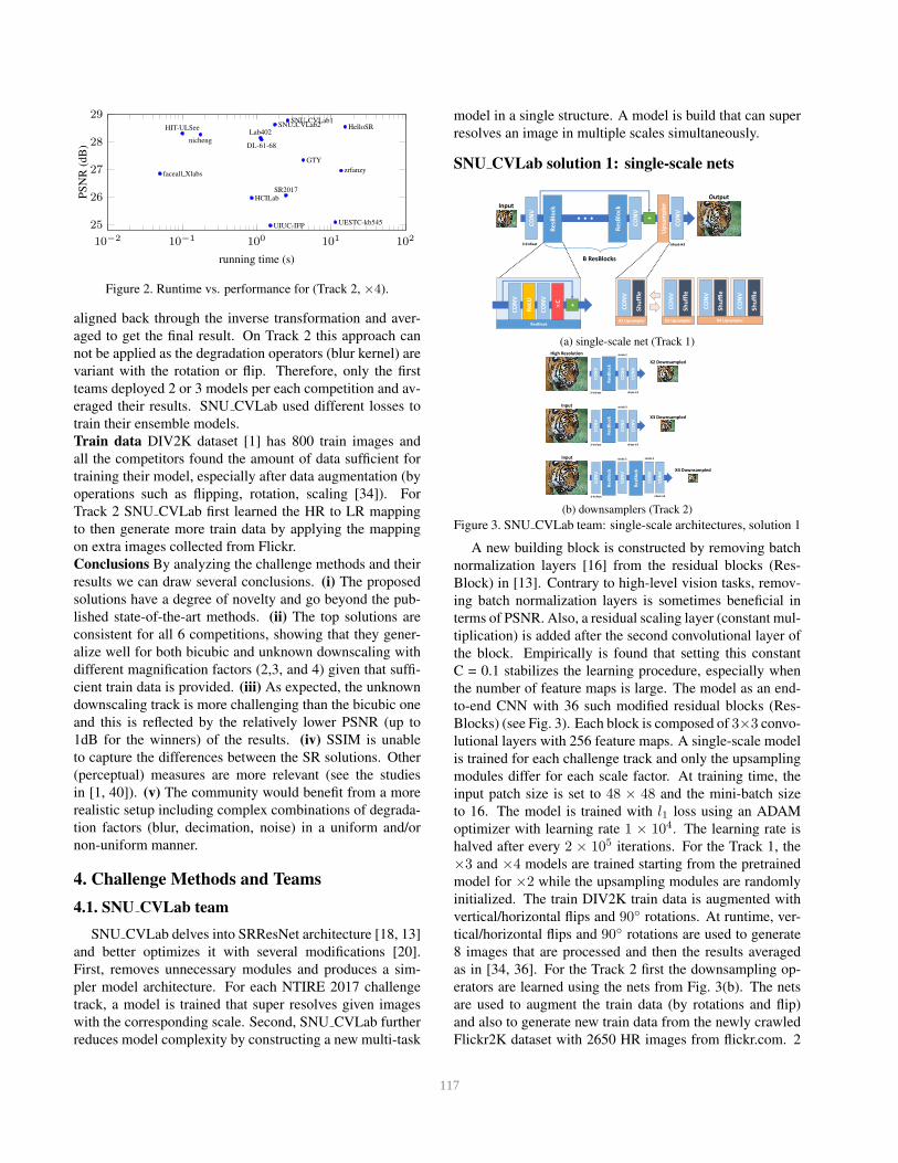
Runtime / efficiency In Figs. 1& 2 we plot runtime per im-

age vs. achieved PSNR performance for two competitions.

HIT-ULSee solution is the most efficient, it gives the best

trade-off between runtime and quality of the results. It runs

in 0.1s for ×4, on Titan X Pascal GPU while being only

0.5dB below the best reported result of SNU CVLab which

is much slower: 20s on (Track1,×4) and 2.6s on (Track 2,

×4).

10−2

10−1

100

101

102

103

32

33

34

35 SNU CVLab1SNU CVLab2

HelloSRLab402

VICLab UIUC-IFPHIT-ULSee I hate mosaicGTY

faceall Xlabs SR2017SDQ SRHCILabiPAL

zrfanzy

WSDSR

running time (s)

PS

NR

(dB

)

Figure 1. Runtime vs. performance for (Track 1, ×2).

Ensembles and fusion Only SNU CVLab, HelloSR,

UIUC-IFP, and ‘I hate mosaic’ used ensembles of meth-

ods/results to boost their performance. The common ap-

proach is the enhanced prediction or multi-view process-

ing [34, 36] which assumes flips and rotations (in 90◦ steps)

of the input LR image to obtain 4 or 8 HR results that are

116

10−2

10−1

100

101

102

25

26

27

28

29SNU CVLab1

SNU CVLab2 HelloSRLab402

UIUC-IFP

HIT-ULSee

nicheng

GTY

DL-61-68

faceall Xlabs

SR2017HCILab

zrfanzy

UESTC-kb545

running time (s)

PS

NR

(dB

)

Figure 2. Runtime vs. performance for (Track 2, ×4).

aligned back through the inverse transformation and aver-

aged to get the final result. On Track 2 this approach can

not be applied as the degradation operators (blur kernel) are

variant with the rotation or flip. Therefore, only the first

teams deployed 2 or 3 models per each competition and av-

eraged their results. SNU CVLab used different losses to

train their ensemble models.

Train data DIV2K dataset [1] has 800 train images and

all the competitors found the amount of data sufficient for

training their model, especially after data augmentation (by

operations such as flipping, rotation, scaling [34]). For

Track 2 SNU CVLab first learned the HR to LR mapping

to then generate more train data by applying the mapping

on extra images collected from Flickr.

Conclusions By analyzing the challenge methods and their

results we can draw several conclusions. (i) The proposed

solutions have a degree of novelty and go beyond the pub-

lished state-of-the-art methods. (ii) The top solutions are

consistent for all 6 competitions, showing that they gener-

alize well for both bicubic and unknown downscaling with

different magnification factors (2,3, and 4) given that suffi-

cient train data is provided. (iii) As expected, the unknown

downscaling track is more challenging than the bicubic one

and this is reflected by the relatively lower PSNR (up to

1dB for the winners) of the results. (iv) SSIM is unable

to capture the differences between the SR solutions. Other

(perceptual) measures are more relevant (see the studies

in [1, 40]). (v) The community would benefit from a more

realistic setup including complex combinations of degrada-

tion factors (blur, decimation, noise) in a uniform and/or

non-uniform manner.

4. Challenge Methods and Teams

4.1. SNU CVLab team

SNU CVLab delves into SRResNet architecture [18, 13]

and better optimizes it with several modifications [20].

First, removes unnecessary modules and produces a sim-

pler model architecture. For each NTIRE 2017 challenge

track, a model is trained that super resolves given images

with the corresponding scale. Second, SNU CVLab further

reduces model complexity by constructing a new multi-task

model in a single structure. A model is build that can super

resolves an image in multiple scales simultaneously.

SNU CVLab solution 1: single­scale nets

Re

sBlo

ck

CO

NV

• • • +

CO

NV

B ResBlocks

Input

Output

CO

NV

3→nFeat nFeat→3

CO

NV

Sh

uff

le

X3 Upsampler

CO

NV

Sh

uff

le

CO

NV

Sh

uff

le

X4 Upsampler

Up

sam

ple

r

Re

sBlo

ck

CO

NV

Re

LU

CO

NV ×C

ResBlock

+

CO

NV

Sh

uff

le

X2 Upsampler

(a) single-scale net (Track 1)

CO

NV

CO

NV

High Resolution

X2 Downsampled

CO

NV

nFeat→33→nFeat

stride 2

CO

NV

CO

NV

Input

CO

NV

nFeat→33→nFeat

stride 3

CO

NV

CO

NV

Input

CO

NV

nFeat→33→nFeat

stride 2

CO

NV

stride 2

Re

sBlo

ckR

esB

lock

Re

sBlo

ck

Re

sBlo

ck

X3 Downsampled

X4 Downsampled

(b) downsamplers (Track 2)

Figure 3. SNU CVLab team: single-scale architectures, solution 1

A new building block is constructed by removing batch

normalization layers [16] from the residual blocks (Res-

Block) in [13]. Contrary to high-level vision tasks, remov-

ing batch normalization layers is sometimes beneficial in

terms of PSNR. Also, a residual scaling layer (constant mul-

tiplication) is added after the second convolutional layer of

the block. Empirically is found that setting this constant

C = 0.1 stabilizes the learning procedure, especially when

the number of feature maps is large. The model as an end-

to-end CNN with 36 such modified residual blocks (Res-

Blocks) (see Fig. 3). Each block is composed of 3×3 convo-

lutional layers with 256 feature maps. A single-scale model

is trained for each challenge track and only the upsampling

modules differ for each scale factor. At training time, the

input patch size is set to 48 × 48 and the mini-batch size

to 16. The model is trained with l1 loss using an ADAM

optimizer with learning rate 1 × 104. The learning rate is

halved after every 2 × 105 iterations. For the Track 1, the

×3 and ×4 models are trained starting from the pretrained

model for ×2 while the upsampling modules are randomly

initialized. The train DIV2K train data is augmented with

vertical/horizontal flips and 90◦ rotations. At runtime, ver-

tical/horizontal flips and 90◦ rotations are used to generate

8 images that are processed and then the results averaged

as in [34, 36]. For the Track 2 first the downsampling op-

erators are learned using the nets from Fig. 3(b). The nets

are used to augment the train data (by rotations and flip)

and also to generate new train data from the newly crawled

Flickr2K dataset with 2650 HR images from flickr.com. 2

117

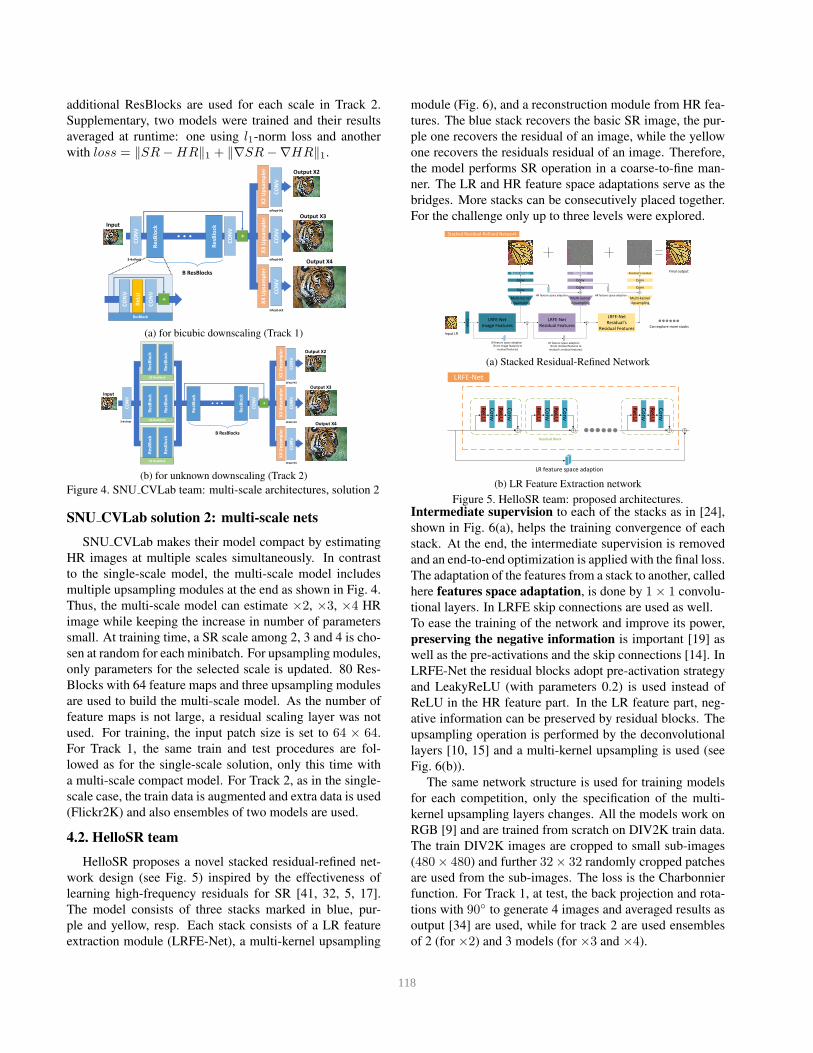
additional ResBlocks are used for each scale in Track 2.

Supplementary, two models were trained and their results

averaged at runtime: one using l1-norm loss and another

with loss = ‖SR−HR‖1 + ‖∇SR−∇HR‖1.

Re

sBlo

ck

CO

NV

• • • +

Input

Output X2

CO

NV

3→nFeat

CO

NV

Re

LU

CO

NV

ResBlock

+

Re

sBlo

ck

CO

NV

nFeat→3

X2

Up

sam

ple

r

CO

NV

nFeat→3X

3 U

psa

mp

ler

CO

NV

nFeat→3

X4

Up

sam

ple

r

Output X3

Output X4

B ResBlocks

(a) for bicubic downscaling (Track 1)

Re

sBlo

ck

CO

NV

• • • +

Input

Output X2

CO

NV

Re

sBlo

ck

CO

NV

nFeat→3

X2

Up

sam

ple

r

CO

NV

nFeat→3

X3

Up

sam

ple

r

CO

NV

nFeat→3

X4

Up

sam

ple

r

Output X3

Output X4

B ResBlocks

3→nFeat

Re

sBlo

ck

Re

sBlo

ck

X3 ResBlock

Re

sBlo

ck

Re

sBlo

ck

X4 ResBlock

Re

sBlo

ck

Re

sBlo

ck

X2 ResBlock

(b) for unknown downscaling (Track 2)

Figure 4. SNU CVLab team: multi-scale architectures, solution 2

SNU CVLab solution 2: multi­scale nets

SNU CVLab makes their model compact by estimating

HR images at multiple scales simultaneously. In contrast

to the single-scale model, the multi-scale model includes

multiple upsampling modules at the end as shown in Fig. 4.

Thus, the multi-scale model can estimate ×2, ×3, ×4 HR

image while keeping the increase in number of parameters

small. At training time, a SR scale among 2, 3 and 4 is cho-

sen at random for each minibatch. For upsampling modules,

only parameters for the selected scale is updated. 80 Res-

Blocks with 64 feature maps and three upsampling modules

are used to build the multi-scale model. As the number of

feature maps is not large, a residual scaling layer was not

used. For training, the input patch size is set to 64 × 64.

For Track 1, the same train and test procedures are fol-

lowed as for the single-scale solution, only this time with

a multi-scale compact model. For Track 2, as in the single-

scale case, the train data is augmented and extra data is used

(Flickr2K) and also ensembles of two models are used.

4.2. HelloSR team

HelloSR proposes a novel stacked residual-refined net-

work design (see Fig. 5) inspired by the effectiveness of

learning high-frequency residuals for SR [41, 32, 5, 17].

The model consists of three stacks marked in blue, pur-

ple and yellow, resp. Each stack consists of a LR feature

extraction module (LRFE-Net), a multi-kernel upsampling

module (Fig. 6), and a reconstruction module from HR fea-

tures. The blue stack recovers the basic SR image, the pur-

ple one recovers the residual of an image, while the yellow

one recovers the residuals residual of an image. Therefore,

the model performs SR operation in a coarse-to-fine man-

ner. The LR and HR feature space adaptations serve as the

bridges. More stacks can be consecutively placed together.

For the challenge only up to three levels were explored.

Stacked Residual-Refined Network

LRFE-Net

Image Features

Multi-kernel

Upsampling

LR feature space adaption

Conv

Conv

Basic Image

LRFE-Net

Residual Features

Multi-kernel

Upsampling

LR feature space adaption

Conv

Conv

Residual

(From image features to

residual features)

HR feature space adaption

LRFE-Net

Residual s

Residual Features

Multi-kernel

Upsampling

Conv

Conv

Residual s residual

HR feature space adaption

Final output

Can explore more stacks

Input LR

(From residual features to

residual s residual features)

Co

nv

(a) Stacked Residual-Refined Network

LRFE-Net

Co

nv

Re

LU

Co

nv

Re

LU

Residual Block

Co

nv

Re

LU

Co

nv

Re

LU

Co

nv

Re

LU

Co

nv

Re

LU

LR feature space adaption

(b) LR Feature Extraction network

Figure 5. HelloSR team: proposed architectures.Intermediate supervision to each of the stacks as in [24],

shown in Fig. 6(a), helps the training convergence of each

stack. At the end, the intermediate supervision is removed

and an end-to-end optimization is applied with the final loss.

The adaptation of the features from a stack to another, called

here features space adaptation, is done by 1× 1 convolu-

tional layers. In LRFE skip connections are used as well.

To ease the training of the network and improve its power,

preserving the negative information is important [19] as

well as the pre-activations and the skip connections [14]. In

LRFE-Net the residual blocks adopt pre-activation strategy

and LeakyReLU (with parameters 0.2) is used instead of

ReLU in the HR feature part. In the LR feature part, neg-

ative information can be preserved by residual blocks. The

upsampling operation is performed by the deconvolutional

layers [10, 15] and a multi-kernel upsampling is used (see

Fig. 6(b)).

The same network structure is used for training models

for each competition, only the specification of the multi-

kernel upsampling layers changes. All the models work on

RGB [9] and are trained from scratch on DIV2K train data.

The train DIV2K images are cropped to small sub-images

(480× 480) and further 32× 32 randomly cropped patches

are used from the sub-images. The loss is the Charbonnier

function. For Track 1, at test, the back projection and rota-

tions with 90◦ to generate 4 images and averaged results as

output [34] are used, while for track 2 are used ensembles

of 2 (for ×2) and 3 models (for ×3 and ×4).

118

Intermediate supervision

LRFE-Net

Image Features

Multi-kernel

Upsampling

LR feature space adaption

Conv

Conv

Basic Image

LRFE-Net

Residual Features

Multi-kernel

Upsampling

LR feature space adaption

Conv

Conv

Residual

(From image features to

residual features)

HR feature space adaption

LRFE-Net

Residual s

Residual Features

Multi-kernel

Upsampling

Conv

Conv

Residual s residual

HR feature space adaption

Input LR

(From residual features to

residual s residual features)

Co

nv

Ground-Truth

loss

loss

loss

(a) intermediate supervision

LRFE-Net

Image Features

LR feature space adaption(From image features to

residual features)

LRFE-Net

Image Features

Subtraction has the similar performance,

which means outputs are residual features

K=4

K=8

K=6Multi-kernel

Upsampling

LR feature space adaptionMulti-kernel Upsampling

different kernel size

(b) multi kernel upsampling and feature space adaptation

Figure 6. HelloSR team: supervision, upsampling and adaptation.

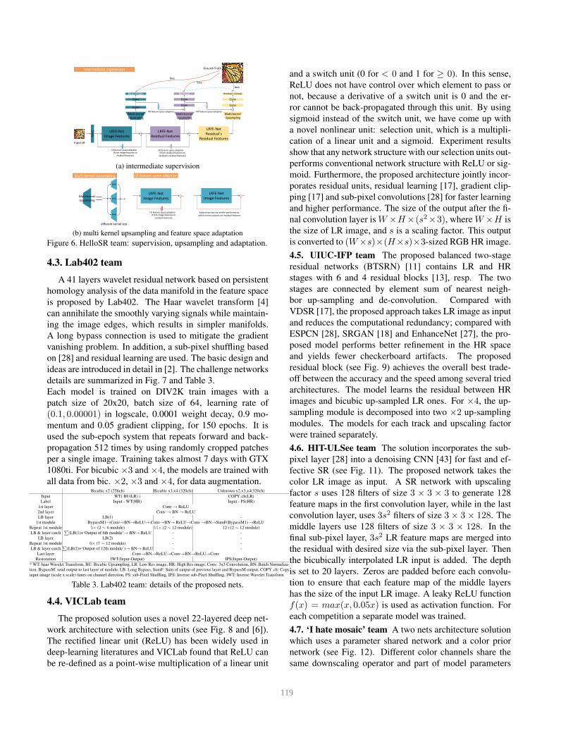
4.3. Lab402 team

A 41 layers wavelet residual network based on persistent

homology analysis of the data manifold in the feature space

is proposed by Lab402. The Haar wavelet transform [4]

can annihilate the smoothly varying signals while maintain-

ing the image edges, which results in simpler manifolds.

A long bypass connection is used to mitigate the gradient

vanishing problem. In addition, a sub-pixel shuffling based

on [28] and residual learning are used. The basic design and

ideas are introduced in detail in [2]. The challenge networks

details are summarized in Fig. 7 and Table 3.

Each model is trained on DIV2K train images with a

patch size of 20x20, batch size of 64, learning rate of

(0.1, 0.00001) in logscale, 0.0001 weight decay, 0.9 mo-

mentum and 0.05 gradient clipping, for 150 epochs. It is

used the sub-epoch system that repeats forward and back-

propagation 512 times by using randomly cropped patches

per a single image. Training takes almost 7 days with GTX

1080ti. For bicubic ×3 and ×4, the models are trained with

all data from bic. ×2, ×3 and ×4, for data augmentation.Bicubic x2 (256ch) Bicubic x3,x4 (320ch) Unknown x2,x3,x4(320ch)

Input WT( BU(LR) ) COPY ch(LR)

Label Input - WT(HR) Input - PS(HR)

1st layer Conv → ReLU

2nd layer Conv → BN → ReLU

LB layer LB(1) - -

1st module BypassM1→Conv→BN→ReLU→ Conv→BN→ ReLU→Conv →BN→SumF(BypassM1) →ReLU

Repeat 1st module 5× (2 ∼ 6 module) 11× (2 ∼ 12 module) 12×(2 ∼ 12 module)

LB & layer catch∑

(LB(1)+‘Output of 6th module’→ BN→ ReLU - -

LB layer LB(2) - -

Repeat 1st module 6× (7 ∼ 12 module) - -

LB & layer catch∑

(LB(2)+‘Output of 12th module’)→ BN→ ReLU - -

Last layer Conv→BN→ReLU→Conv→BN→ReLU→Conv

Restoration IWT(Input-Output) IPS(Input-Output)

* WT: haar Wavelet Transform, BU: Bicubic Upsampling, LR: Low Res image, HR: High Res image, Conv: 3x3 Convolution, BN: Batch Normaliza-

tion, BypassM: send output to last layer of module, LB: Long Bypass, SumF: Sum of output of previous layer and BypassM output, COPY ch: Copy

input image (scale x scale) times on channel direction, PS: sub-Pixel Shuffling, IPS: Inverse sub-Pixel Shuffling, IWT: Inverse Wavelet Transform

Table 3. Lab402 team: details of the proposed nets.

4.4. VICLab team

The proposed solution uses a novel 22-layered deep net-

work architecture with selection units (see Fig. 8 and [6]).

The rectified linear unit (ReLU) has been widely used in

deep-learning literatures and VICLab found that ReLU can

be re-defined as a point-wise multiplication of a linear unit

and a switch unit (0 for < 0 and 1 for ≥ 0). In this sense,

ReLU does not have control over which element to pass or

not, because a derivative of a switch unit is 0 and the er-

ror cannot be back-propagated through this unit. By using

sigmoid instead of the switch unit, we have come up with

a novel nonlinear unit: selection unit, which is a multipli-

cation of a linear unit and a sigmoid. Experiment results

show that any network structure with our selection units out-

performs conventional network structure with ReLU or sig-

moid. Furthermore, the proposed architecture jointly incor-

porates residual units, residual learning [17], gradient clip-

ping [17] and sub-pixel convolutions [28] for faster learning

and higher performance. The size of the output after the fi-

nal convolution layer is W ×H×(s2×3), where W ×H is

the size of LR image, and s is a scaling factor. This output

is converted to (W×s)×(H×s)×3-sized RGB HR image.

4.5. UIUC-IFP team The proposed balanced two-stage

residual networks (BTSRN) [11] contains LR and HR

stages with 6 and 4 residual blocks [13], resp. The two

stages are connected by element sum of nearest neigh-

bor up-sampling and de-convolution. Compared with

VDSR [17], the proposed approach takes LR image as input

and reduces the computational redundancy; compared with

ESPCN [28], SRGAN [18] and EnhanceNet [27], the pro-

posed model performs better refinement in the HR space

and yields fewer checkerboard artifacts. The proposed

residual block (see Fig. 9) achieves the overall best trade-

off between the accuracy and the speed among several tried

architectures. The model learns the residual between HR

images and bicubic up-sampled LR ones. For ×4, the up-

sampling module is decomposed into two ×2 up-sampling

modules. The models for each track and upscaling factor

were trained separately.

4.6. HIT-ULSee team The solution incorporates the sub-

pixel layer [28] into a denoising CNN [43] for fast and ef-

fective SR (see Fig. 11). The proposed network takes the

color LR image as input. A SR network with upscaling

factor s uses 128 filters of size 3 × 3 × 3 to generate 128

feature maps in the first convolution layer, while in the last

convolution layer, uses 3s2 filters of size 3× 3× 128. The

middle layers use 128 filters of size 3 × 3 × 128. In the

final sub-pixel layer, 3s2 LR feature maps are merged into

the residual with desired size via the sub-pixel layer. Then

the bicubically interpolated LR input is added. The depth

is set to 20 layers. Zeros are padded before each convolu-

tion to ensure that each feature map of the middle layers

has the size of the input LR image. A leaky ReLU function

f(x) = max(x, 0.05x) is used as activation function. For

each competition a separate model was trained.

4.7. ‘I hate mosaic’ team A two nets architecture solution

which uses a parameter shared network and a color prior

network (see Fig. 12). Different color channels share the

same downscaling operator and part of model parameters

119

(a) Bicubic ×2 (b) Bicubic ×3,×4 (320ch) (c) Unknown ×2,×3,×4 (320ch)

Figure 7. Lab402 team: the proposed nets for challenge tasks.

Figure 8. VICLab team: proposed network with selection unit.

Figure 9. UIUC-IFP team:

proposed residual block.Figure 10. Resonance team:

an inception ResNet block.

Figure 11. HIT-ULSee team: proposed CNN architecture.

(a) Parameter shared net

(b) ResBlock in parameter shared net (c) ResBlock in color prior net

Figure 12. ‘I hate mosaic’ team: nets and residual blocks.

to exploit cross channel correlation constraints [23]. An-

other net is deployed to learn the difference among different

color channels and color prior. Upsampling module upscale

feature maps from LR to HR via depth-to-space convolu-

tion (aka sub-pixel convolution). A shallow and extremely

simple sub-network is used to reduce the low-frequent re-

dundancy [31] and to accelerate training. The color prior

network has 6 residual blocks. This objective function is

robustified (includes a variant of MSE and a differentiable

variant of l1 norm) to deal with the outliers in training.

4.8. nicheng team A SRResNet [18]-based solution with

a couple of modifications (see Fig. 13. For ×4, the nearest-

neighbour interpolation layer replaces the sub-pixel layer,

otherwise the sub-pixel layer would cause the checkerboard

pattern of artifacts [25]. Also the input is interpolated and

added to the network output as in [17]. ×3 model uses the

pixel shift method to up-sample the image.

Figure 13. nicheng team: SRResNet modif. models for ×3 & ×4.

4.9. GTY team Four modified VDSR nets [17] (PReLU

instead of ReLu, RGB channels instead of one) are stacked

and their outputs are linearly combined to obtain the final

HR output as shown in Fig. 14.

Figure 14. GTY team: multi-fused deep network based on VDSR.

4.10. DL-61-86 A two-stage solution: deblurring then

SR of the LR blur-free images. A blind deconvolution

method [39] estimated the blur kernel on each train image

and the average blur kernel was used for deblurring. Af-

ter deblurring, a SRResNet [18, 28] learned the mapping to

HR using both MSE loss and a perceptual loss. The train-

ing employed the cyclical learning rate strategy [29] and in-

spired by [37] used both train images and re-scaled images

120

to enhance the generality of the model for local structures

of different scales in natural images.

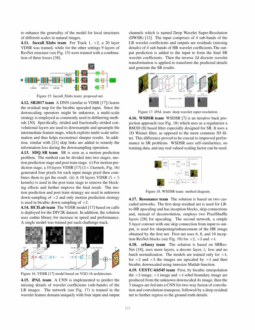
4.11. faceall Xlabs team For Track 1, ×2, a 20 layer

VDSR was trained, while for the other settings 9 layers of

ResNet structure (see Fig. 15) were trained with a combina-

tion of three losses [38].

Figure 15. faceall Xlabs team: proposed net.

4.12. SR2017 team A DNN (similar to VDSR [17]) learns

the residual map for the bicubic upscaled input. Since the

downscaling operators might be unknown, a multi-scale

strategy is employed as commonly used in deblurring meth-

ods [30]. Specifically, strided and fractionally-strided con-

volutional layers are used to downsample and upsample the

intermediate feature maps, which exploits multi-scale infor-

mation and thus helps reconstruct sharper results. In addi-

tion, similar with [21] skip links are added to remedy the

information loss during the downsampling operation.

4.13. SDQ SR team SR is seen as a motion prediction

problem. The method can be divided into two stages, mo-

tion prediction stage and post train stage. (i) For motion pre-

diction stage, a 10 layers VDSR [17] (3×3 kernels, Fig. 16)

generated four pixels for each input image pixel then com-

bines them to get the result. (ii) A 10 layers VDSR (5 × 5kernels) is used in the post train stage to remove the block-

ing effects and further improve the final result. The mo-

tion prediction and post train strategy are used in unknown

down-sampling of ×2 and only motion prediction strategy

is used in bicubic down-sampling of ×2.

4.14. HCILab team The VDSR model [17] based on caffe

is deployed for the DIV2K dataset. In addition, the solution

uses cudnn library for increase in speed and performance.

A single model was trained per each challenge track.

Figure 16. VDSR [17] model based on VGG-16 architecture.

4.15. iPAL team A CNN is implemented to predict the

missing details of wavelet coefficients (sub-bands) of the

LR images. The network (see Fig. 17) is trained in the

wavelet feature domain uniquely with four input and output

channels which is named Deep Wavelet Super-Resolution

(DWSR) [12]. The input comprises of 4 sub-bands of the

LR wavelet coefficients and outputs are residuals (missing

details) of 4 sub-bands of HR wavelet coefficients.The out-

put prediction is added to the input to form the final SR

wavelet coefficients. Then the inverse 2d discrete wavelet

transformation is applied to transform the predicted details

and generate the SR results.

0 50 100 150 200 250 3000

0.1

0.2

0.4

0.5

0.6

0.7

Histogram of ∆SB

LR SR

2dDWT

Input Conv. 1 Conv. 2 Conv. N Output

2dIDWT

LRSB

{LA, LV, LH, LD}4 input channels

∆SB

{∆A, ∆V, ∆H, ∆D}4 output channels

LRSB + ∆SB

SRSB

{SA, SV, SH, SD}

b bbb bb+

Figure 17. iPAL team: deep wavelet super-resolution.

4.16. WSDSR team WSDSR [7] is an iterative back pro-

jection approach (see Fig. 18) which uses as a regularizer a

BM3D [8] based filter especially designed for SR. It uses a

1D Wiener filter, as opposed to the more common 3D fil-

ter. This difference proved to be crucial to improved perfor-

mance in SR problems. WSDSR uses self-similarities, no

training data, and any real valued scaling factor can be used.

Figure 18. WSDSR team: method diagram.

4.17. Resonance team The solution is based on two cas-

caded networks. The first deep residual net is used for LR-

to-HR upscaling and has inception blocks, skip connections

and, instead of deconvolution, employs two PixelShuffle

layers [28] for upscaling. The second network, a simple

5-layer convnet with one skip connection from input to out-

put, is used for sharpening/enhancement of the HR image

obtained by the first net. First net uses 6, 8, and 10 incep-

tion ResNet blocks (see Fig. 10) for ×2, ×3 and ×4.

4.18. zrfanzy team The solution is based on SRRes-

Net [18], uses more layers, a deconv layer, l1 loss and no

batch normalization. The models are trained only for ×4,

for ×2 and ×3 the images are upscaled by ×4 and then

bicubic downscaled using imresize Matlab function.

4.19. UESTC-kb545 team First, by bicubic interpolation

the ×2 image, ×4 image and ×4 sobel boundary image are

produced from the unknown downscaled 4x image, then the

3 images are fed into a CNN for two-way fusion of convolu-

tion and convolution-transpose, followed by a deep residual

net to further regress to the ground truth details.

121

Acknowledgements

We thank the NTIRE 2017 sponsors: NVIDIA Corp.,

SenseTime Group Ltd., Twitter Inc., Google Inc., and ETH

Zurich.

A. Teams and affiliations

NTIRE2017 team

Title: NTIRE 2017 Challenge on example-based single

image super-resolution

Members: Radu Timofte 1,2

(radu.timofte@vision.ee.ethz.ch), Eirikur Agustsson 1, Luc

Van Gool 1,3, Ming-Hsuan Yang 4, Lei Zhang 5

Affiliations:1 Computer Vision Lab, ETH Zurich, Switzerland2 Merantix GmbH, Germany3 ESAT, KU Leuven, Belgium4 University of California at Merced, US5 Polytechnic University of Hong Kong, China

A.1. SNU CVLab team

Title: Enhanced Deep Residual Networks for Single Image

Super-Resolution

Members:Lim Bee (forestrainee@gmail.com), Sanghyun

Son, Seungjun Nah, Heewon Kim, Kyoung Mu Lee

Affiliation:

CVLab, Seoul National University, Korea

A.2. HelloSR team

Title: Stacked Residual-Refined Network for Super-

Resolution

Members: Xintao Wang 1 (wx016@ie.cuhk.edu.hk), Yapeng

Tian 2 (typ14@mails.tsinghua.edu.cn), Ke Yu 1, Yulun

Zhang 2, Shixiang Wu 2, Chao Dong 3, Liang Lin 3, Yu

Qiao 2, Chen Change Loy 1

Affiliations:1 The Chinese University of Hong Kong2 Shenzhen Institutes of Advanced Technology, Chinese

Academy of Sciences3 SenseTime

A.3. Lab402 team

Title: Very Deep Residual Learning for SISR - Persistent

Homology Guided Manifold Simplification

Members: Woong Bae (iorism@kaist.ac.kr), Jaejun Yoo,

Yoseob Han, Jong Chul Ye

Affiliation:

Korea Ad. Inst. of Science & Technology (KAIST)

A.4. VICLab team

Title: A Deep Convolutional Neural Network with Selec-

tion Units for Super-Resolution

Members: Jae-Seok Choi (jschoi14@kaist.ac.kr),

Munchurl Kim

Affiliation:

Korea Ad. Inst. of Science & Technology (KAIST)

A.5. UIUC­IFP team

Title: Balanced Two-Stage Residual Networks for Image

Super-Resolution

Members: Yuchen Fan (yuchenf4@illinois.edu), Jiahui

Yu, Wei Han, Ding Liu, Haichao Yu, Zhangyang Wang,

Honghui Shi, Xinchao Wang, Thomas S. Huang

Affiliation:

IFP, University of Illinois at Urbana-Champaign, US

A.6. HIT­ULSee team

Title: Accelerated very deep denoising convolutional

neural network for image super-resolution

Members: Yunjin Chen 1(chenyunjin nudt@hotmail.com),

Kai Zhang 2, Wangmeng Zuo 2

Affiliations:1 ULSee Inc.2 Harbin Institute of Technology, China

A.7. ‘I hate mosaic’ team

Title: Low-frequency Redundancy Reduction and Color

Constraint for Color Image Super-resolution

Members: Zhimin Tang (tangzhimin@stu.xmu.edu.cn),

Linkai Luo, Shaohui Li, Min Fu, Lei Cao

Affiliation:

Department of Automation, Xiamen University, China

A.8. nicheng team

Title: Modified SRResNet

Members: Wen Heng (wenheng@pku.edu.cn)

Affiliation:

Peking University, China

A.9. GTY team

Title: Multi-fused Deep Network for Image SR

Members: Giang Bui (giangbui0816@gmail.com), Truc

Le, Ye Duan

Affiliation:

University of Missouri, Columbia, US

A.10. DL­61­86

Title: A two-stage super-resolution method under un-

known downsampling op- erations

Members: Dacheng Tao 5 (dacheng.tao@sydney.edu.au),

Ruxin Wang 1,2, Xu Lin 3, Jianxin Pang 4

Affiliations:1 CSIC(Kunming) Linghu Eviromental Intelligent Sensing

122

Technologies Co., Ltd2 Yunshangyun Artificial Intelligence Institute3 ShenzhenUnion Vision InnovationsTechnology Co., Ltd4 UBTECH ROBOTICS CORP5 UBTech Sydney Artificial Intelligence Institute, Univer-

sity of Sydney

A.11. faceall Xlabs team

Title: Fast and Accurate Image Super-Resolution Using A

Combined Loss

Members: Jinchang Xu (xjc1@bupt.edu.cn), Yu Zhao

Affiliation:

Beijing University of Posts and Telecommunications, China

A.12. SR2017 team

Title: Blind Super-Resolution with Multi-Scale Convolu-

tional Neural Network

Members: Xiangyu Xu (xuxiangyu2014@gmail.com), Jin-

shan Pan, Deqing Sun, Yujin Zhang, Ming-Hsuan Yang

Affiliations:

Electronic Engineering, Tsinghua University, China

EECS, University of California, Merced, US

A.13. SDQ SR team

Title: Supervised Image SR as Motion Prediction

Members: Xibin Song 1 (song.sducg@gmail.com), Yuchao

Dai 2, Xueying Qin 1

Affiliations:1 Shandong University, China2 The Australian National University, Australia

A.14. HCILab team

Title: Elevate Image Super-Resolution Using Very Deep

Convolutional Networks

Member: Xuan-Phung Huynh (phunghx@gmail.com)

Affiliation:

Sejong University, Seoul, Korea

A.15. iPAL team

Title: Deep Wavelet Prediction for Image Super-resolution

Members: Tiantong Guo (tong.renly@gmail.com), Hojjat

Seyed Mousavi, Tiep Huu Vu, Vishal Monga

Affiliation:

School of Electrical Engineering and Computer Science,

The Pennsylvania State University, US

A.16. WSDSR team

Title: Single Image Super-Resolution based on Wiener Fil-

ter in Similarity Domain

Members: Cristovao Cruz (cristovao.antunescruz@tut.fi),

Karen Egiazarian, Vladimir Katkovnik, Rakesh Mehta

Affiliation:

Tampere University of Technology, Finland

A.17. Resonance team

Title: MultiSRNet

Members: Arnav Kumar Jain (arnavkj95@iitkgp.ac.in),

Abhinav Agarwalla, Ch V Sai Praveen

Affiliation:

Indian Institute of Technology Kharagpur, India

A.18. zrfanzy team

Title: Deep Learning Approach for Image Super Resolu-

tion

Member: Ruofan Zhou (zrfanzy@gmail.com)

Affiliation:

EPFL, Switzerland

A.19. UESTC­kb545 team

Title: Two-way RefineNet for image super-resolution

Members: Hongdiao Wen (uestc wen@outlook.com), Che

Zhu, Zhiqiang Xia, Zhengtao Wang, Qi Guo

Affiliation:

School of Electronic Engineering/Center for Robotics, Uni-

versity of Electronic Science and Technology of China

(UESTC), Chengdu

References

[1] E. Agustsson and R. Timofte. NTIRE 2017 challenge on

single image super-resolution: Dataset and study. In The

IEEE Conference on Computer Vision and Pattern Recogni-

tion (CVPR) Workshops, July 2017.

[2] W. Bae, J. Yoo, and J. C. Ye. Beyond deep residual learning

for image restoration: Persistent homology-guided manifold

simplification. In The IEEE Conference on Computer Vision

and Pattern Recognition (CVPR) Workshops, July 2017.

[3] M. Bevilacqua, A. Roumy, C. Guillemot, and M. line Al-

beri Morel. Low-complexity single-image super-resolution

based on nonnegative neighbor embedding. In Proceed-

ings of the British Machine Vision Conference, pages 135.1–

135.10. BMVA Press, 2012.

[4] M. Bianchini and F. Scarselli. On the complexity of neu-

ral network classifiers: A comparison between shallow and

deep architectures. IEEE transactions on neural networks

and learning systems, 25(8):1553–1565, 2014.

[5] J. Bruna, P. Sprechmann, and Y. LeCun. Super-resolution

with deep convolutional sufficient statistics. CoRR,

abs/1511.05666, 2015.

[6] J.-S. Choi and M. Kim. A deep convolutional neural network

with selection units for super-resolution. In The IEEE Con-

ference on Computer Vision and Pattern Recognition (CVPR)

Workshops, July 2017.

[7] C. Cruz, R. Mehta, V. Katkovnik, and K. Egiazarian. Single

image super-resolution based on wiener filter in similarity

domain. arXiv preprint arXiv:1704.04126, 2017.

123

[8] K. Dabov, A. Foi, V. Katkovnik, and K. Egiazarian. Im-

age denoising by sparse 3-d transform-domain collabora-

tive filtering. IEEE Transactions on Image Processing,

16(8):2080–2095, Aug 2007.

[9] C. Dong, C. C. Loy, K. He, and X. Tang. Image

super-resolution using deep convolutional networks. IEEE

Transactions on Pattern Analysis and Machine Intelligence,

38(2):295–307, Feb 2016.

[10] C. Dong, C. C. Loy, and X. Tang. Accelerating the super-

resolution convolutional neural network. In European Con-

ference on Computer Vision, pages 391–407. Springer, 2016.

[11] Y. Fan, H. Shi, J. Yu, D. Liu, W. Han, H. Yu, Z. Wang,

X. Wang, and T. S. Huang. Balanced two-stage residual net-

works for image super-resolution. In The IEEE Conference

on Computer Vision and Pattern Recognition (CVPR) Work-

shops, July 2017.

[12] T. Guo, H. S. Mousavi, T. H. Vu, and V. Monga. Deep

wavelet prediction for image super-resolution. In The IEEE

Conference on Computer Vision and Pattern Recognition

(CVPR) Workshops, July 2017.

[13] K. He, X. Zhang, S. Ren, and J. Sun. Deep residual learning

for image recognition. In The IEEE Conference on Computer

Vision and Pattern Recognition (CVPR), June 2016.

[14] K. He, X. Zhang, S. Ren, and J. Sun. Identity mappings in

deep residual networks. In European Conference on Com-

puter Vision, pages 630–645. Springer, 2016.

[15] T.-W. Hui, C. C. Loy, and X. Tang. Depth map super-

resolution by deep multi-scale guidance. In European Con-

ference on Computer Vision, pages 353–369. Springer, 2016.

[16] S. Ioffe and C. Szegedy. Batch normalization: Accelerating

deep network training by reducing internal covariate shift.

In F. Bach and D. Blei, editors, Proceedings of the 32nd In-

ternational Conference on Machine Learning, volume 37 of

Proceedings of Machine Learning Research, pages 448–456,

Lille, France, 07–09 Jul 2015. PMLR.

[17] J. Kim, J. Kwon Lee, and K. Mu Lee. Accurate image super-

resolution using very deep convolutional networks. In The

IEEE Conference on Computer Vision and Pattern Recogni-

tion (CVPR), June 2016.

[18] C. Ledig, L. Theis, F. Huszar, J. Caballero, A. P. Aitken,

A. Tejani, J. Totz, Z. Wang, and W. Shi. Photo-realistic

single image super-resolution using a generative adversarial

network. CoRR, abs/1609.04802, 2016.

[19] Y. Liang, R. Timofte, J. Wang, Y. Gong, and N. Zheng. Sin-

gle image super resolution-when model adaptation matters.

arXiv preprint arXiv:1703.10889, 2017.

[20] B. Lim, S. Son, H. Kim, S. Nah, and K. M. Lee. Enhanced

deep residual networks for single image super-resolution.

In The IEEE Conference on Computer Vision and Pattern

Recognition (CVPR) Workshops, July 2017.

[21] J. Long, E. Shelhamer, and T. Darrell. Fully convolutional

networks for semantic segmentation. In The IEEE Confer-

ence on Computer Vision and Pattern Recognition (CVPR),

June 2015.

[22] D. Martin, C. Fowlkes, D. Tal, and J. Malik. A database of

human segmented natural images and its application to eval-

uating segmentation algorithms and measuring ecological

statistics. In Computer Vision, 2001. ICCV 2001. Proceed-

ings. Eighth IEEE International Conference on, volume 2,

pages 416–423. IEEE, 2001.

[23] H. S. Mousavi and V. Monga. Sparsity-based color im-

age super resolution via exploiting cross channel constraints.

CoRR, abs/1610.01066, 2016.

[24] A. Newell, K. Yang, and J. Deng. Stacked Hourglass Net-

works for Human Pose Estimation, pages 483–499. Springer

International Publishing, Cham, 2016.

[25] A. Odena, V. Dumoulin, and C. Olah. Deconvolution and

checkerboard artifacts. Distill, 1(10):e3, 2016.

[26] O. Russakovsky, J. Deng, H. Su, J. Krause, S. Satheesh,

S. Ma, Z. Huang, A. Karpathy, A. Khosla, M. Bernstein,

A. C. Berg, and L. Fei-Fei. ImageNet Large Scale Visual

Recognition Challenge. International Journal of Computer

Vision (IJCV), 115(3):211–252, 2015.

[27] M. S. M. Sajjadi, B. Scholkopf, and M. Hirsch. Enhancenet:

Single image super-resolution through automated texture

synthesis. CoRR, abs/1612.07919, 2016.

[28] W. Shi, J. Caballero, F. Huszar, J. Totz, A. P. Aitken,

R. Bishop, D. Rueckert, and Z. Wang. Real-time single im-

age and video super-resolution using an efficient sub-pixel

convolutional neural network. In The IEEE Conference

on Computer Vision and Pattern Recognition (CVPR), June

2016.

[29] L. N. Smith. No more pesky learning rate guessing games.

CoRR, abs/1506.01186, 2015.

[30] S. Su, M. Delbracio, J. Wang, G. Sapiro, W. Heidrich, and

O. Wang. Deep video deblurring. CoRR, abs/1611.08387,

2016.

[31] Z. Tang and other. A joint residual networks to reduce the re-

dundancy of convolutional neural networks for image super-

resolution. In under review, 2017.

[32] R. Timofte, V. De Smet, and L. Van Gool. Anchored neigh-

borhood regression for fast example-based super-resolution.

In The IEEE International Conference on Computer Vision

(ICCV), December 2013.

[33] R. Timofte, V. De Smet, and L. Van Gool. A+: Adjusted an-

chored neighborhood regression for fast super-resolution. In

D. Cremers, I. Reid, H. Saito, and M.-H. Yang, editors, Com-

puter Vision – ACCV 2014: 12th Asian Conference on Com-

puter Vision, Singapore, Singapore, November 1-5, 2014,

Revised Selected Papers, Part IV, pages 111–126, Cham,

2014. Springer International Publishing.

[34] R. Timofte, R. Rothe, and L. J. V. Gool. Seven ways to im-

prove example-based single image super resolution. CoRR,

abs/1511.02228, 2015.

[35] Z. Wang, A. C. Bovik, H. R. Sheikh, and E. P. Simoncelli.

Image quality assessment: from error visibility to struc-

tural similarity. IEEE Transactions on Image Processing,

13(4):600–612, April 2004.

[36] Z. Wang, D. Liu, J. Yang, W. Han, and T. Huang. Deep

networks for image super-resolution with sparse prior. In The

IEEE International Conference on Computer Vision (ICCV),

December 2015.

[37] C. Xu, D. Tao, and C. Xu. Multi-view intact space learning.

IEEE Transactions on Pattern Analysis and Machine Intelli-

gence, 37(12):2531–2544, Dec 2015.

124

[38] J. Xu, Y. Zhao, Y. Dong, and H. Bai. Fast and accurate image

super-resolution using a combined loss. In The IEEE Con-

ference on Computer Vision and Pattern Recognition (CVPR)

Workshops, July 2017.

[39] L. Xu and J. Jia. Two-Phase Kernel Estimation for Robust

Motion Deblurring, pages 157–170. Springer Berlin Heidel-

berg, Berlin, Heidelberg, 2010.

[40] C.-Y. Yang, C. Ma, and M.-H. Yang. Single-image super-

resolution: A benchmark. In European Conference on Com-

puter Vision, pages 372–386. Springer, 2014.

[41] J. Yang, J. Wright, T. Huang, and Y. Ma. Image super-

resolution as sparse representation of raw image patches.

In 2008 IEEE Conference on Computer Vision and Pattern

Recognition, pages 1–8, June 2008.

[42] R. Zeyde, M. Elad, and M. Protter. On single image scale-up

using sparse-representations. In Curves and Surfaces: 7th

International Conference, Avignon, France, June 24 - 30,

2010, Revised Selected Papers, pages 711–730, 2012.

[43] K. Zhang, W. Zuo, Y. Chen, D. Meng, and L. Zhang. Be-

yond a gaussian denoiser: Residual learning of deep cnn for

image denoising. IEEE Transactions on Image Processing,

PP(99):1–1, 2017.

125