arX

iv:h

ep-t

h/06

0507

3v3

20

Jun

2006

NSF-KITP-06-31

KUNS-2021

hep-th/0605073

May, 2006

Aspects of Holographic Entanglement Entropy

Shinsei Ryu1 and Tadashi Takayanagi2, 3

1 Kavli Institute for Theoretical Physics, University of California,

Santa Barbara, CA 93106, USA

2 Department of Physics, Kyoto University, Kyoto 606-8502, Japan

Abstract

This is an extended version of our short report hep-th/0603001, where a holo-

graphic interpretation of entanglement entropy in conformal field theories is pro-

posed from AdS/CFT correspondence. In addition to a concise review of relevant

recent progresses of entanglement entropy and details omitted in the earlier let-

ter, this paper includes the following several new results : We give a more direct

derivation of our claim which relates the entanglement entropy with the minimal

area surfaces in the AdS3/CFT2 case as well as some further discussions on higher

dimensional cases. Also the relation between the entanglement entropy and central

charges in 4D conformal field theories is examined. We check that the logarith-

mic part of the 4D entanglement entropy computed in the CFT side agrees with

the AdS5 result at least under a specific condition. Finally we estimate the en-

tanglement entropy of massive theories in generic dimensions by making use of our

proposal.

1e-mail: sryu@kitp.ucsb.edu2e-mail: takayana@gauge.scphys.kyoto-u.ac.jp3Moved from Kavli Institute for Theoretical Physics, University of California, Santa Barbara, CA

93106, USA

Contents1 Introduction 2

2 Basics of Entanglement Entropy 4

2.1 Definition of Entanglement Entropy . . . . . . . . . . . . . . . . . . . . . . . . . . . . . . . . . . . . . . . . 4

2.2 Properties . . . . . . . . . . . . . . . . . . . . . . . . . . . . . . . . . . . . . . . . . . . . . . . . . . . . . . . 5

2.3 Entanglement Entropy in QFTs and Area Law . . . . . . . . . . . . . . . . . . . . . . . . . . . . . . . . . . 6

3 Entanglement Entropy in 2D CFT 7

3.1 How to Compute Entanglement Entropy . . . . . . . . . . . . . . . . . . . . . . . . . . . . . . . . . . . . . . 7

3.2 Derivation of Entanglement Entropy in an Infinitely Long System . . . . . . . . . . . . . . . . . . . . . . . . 9

3.3 Derivation of Entanglement Entropy on a Circle . . . . . . . . . . . . . . . . . . . . . . . . . . . . . . . . . 11

3.4 Derivation of Entanglement Entropy at Finite Temperature . . . . . . . . . . . . . . . . . . . . . . . . . . . 12

3.5 Massive Theories . . . . . . . . . . . . . . . . . . . . . . . . . . . . . . . . . . . . . . . . . . . . . . . . . . . 12

4 Entanglement Entropy in Higher Dimensional CFTs 13

4.1 Entanglement Entropy of d + 1 D Massless Free Fields . . . . . . . . . . . . . . . . . . . . . . . . . . . . . . 14

4.1.1 Rough Estimation . . . . . . . . . . . . . . . . . . . . . . . . . . . . . . . . . . . . . . . . . . . . . . 14

4.1.2 Exact Estimation from Entropic c-function . . . . . . . . . . . . . . . . . . . . . . . . . . . . . . . . 16

4.1.3 Entanglement Entropy of 4D Gauge Field . . . . . . . . . . . . . . . . . . . . . . . . . . . . . . . . . 18

4.2 Entanglement Entropy and Central Charges in 4D CFT . . . . . . . . . . . . . . . . . . . . . . . . . . . . . 19

4.2.1 Entanglement Entropy from Weyl Anomaly . . . . . . . . . . . . . . . . . . . . . . . . . . . . . . . . 20

4.2.2 Entanglement Entropy and Central Charges . . . . . . . . . . . . . . . . . . . . . . . . . . . . . . . . 21

5 Holographic Interpretation 24

5.1 General Proposal . . . . . . . . . . . . . . . . . . . . . . . . . . . . . . . . . . . . . . . . . . . . . . . . . . . 24

5.2 Intuitive Derivation from AdS/CFT . . . . . . . . . . . . . . . . . . . . . . . . . . . . . . . . . . . . . . . . 25

6 Entanglement Entropy in 2D CFT from AdS3 27

6.1 AdS3 Space and UV Cutoff in Dual CFTs . . . . . . . . . . . . . . . . . . . . . . . . . . . . . . . . . . . . . 27

6.2 Geodesics in AdS3 and Entanglement Entropy in CFT2 . . . . . . . . . . . . . . . . . . . . . . . . . . . . . 28

6.3 Calculations in Poincare Coordinates . . . . . . . . . . . . . . . . . . . . . . . . . . . . . . . . . . . . . . . . 29

6.4 Entropy on Multiple Disjoint Intervals . . . . . . . . . . . . . . . . . . . . . . . . . . . . . . . . . . . . . . . 29

6.5 Finite Temperature Cases . . . . . . . . . . . . . . . . . . . . . . . . . . . . . . . . . . . . . . . . . . . . . . 30

6.6 Massive Deformation . . . . . . . . . . . . . . . . . . . . . . . . . . . . . . . . . . . . . . . . . . . . . . . . . 31

7 Entanglement Entropy in CFTd+1 from AdSd+2 32

7.1 General Results . . . . . . . . . . . . . . . . . . . . . . . . . . . . . . . . . . . . . . . . . . . . . . . . . . . . 33

7.1.1 Entanglement Entropy for Straight Belt AS . . . . . . . . . . . . . . . . . . . . . . . . . . . . . . . . 33

7.1.2 Entanglement Entropy for Circular Disk AD . . . . . . . . . . . . . . . . . . . . . . . . . . . . . . . 34

7.1.3 Multiple Loops . . . . . . . . . . . . . . . . . . . . . . . . . . . . . . . . . . . . . . . . . . . . . . . . 36

7.2 Entanglement Entropy in N = 4 SYM from AdS5× S5 . . . . . . . . . . . . . . . . . . . . . . . . . . . . . . 36

7.3 Entanglement Entropy and Central Charges in 4D CFT from AdS5 . . . . . . . . . . . . . . . . . . . . . . . 38

7.4 Entanglement Entropy from AdS4,7×S7,4 in M-theory . . . . . . . . . . . . . . . . . . . . . . . . . . . . . . 39

7.5 Finite Temperature Case . . . . . . . . . . . . . . . . . . . . . . . . . . . . . . . . . . . . . . . . . . . . . . . 41

7.6 Massive Deformations . . . . . . . . . . . . . . . . . . . . . . . . . . . . . . . . . . . . . . . . . . . . . . . . 42

7.6.1 Straight Belt AS . . . . . . . . . . . . . . . . . . . . . . . . . . . . . . . . . . . . . . . . . . . . . . . 42

7.6.2 Circular Disk AD . . . . . . . . . . . . . . . . . . . . . . . . . . . . . . . . . . . . . . . . . . . . . . . 43

7.7 Entanglement Entropy in Some Non-Conformal Theories . . . . . . . . . . . . . . . . . . . . . . . . . . . . . 44

7.7.1 D2-branes Case . . . . . . . . . . . . . . . . . . . . . . . . . . . . . . . . . . . . . . . . . . . . . . . . 45

7.7.2 NS5-branes Case . . . . . . . . . . . . . . . . . . . . . . . . . . . . . . . . . . . . . . . . . . . . . . . 46

8 Conclusions and Discussions 47

1

1 Introduction

When we study properties of a given quantum field theory (QFT), it is common to first

investigate behaviors of correlation functions of local operators in the theory. However,

properties of non-local quantities are equally important, especially for understanding of

its quantum mechanical phase structure. One basic such example of non-local physical

quantities is the Wilson loop operators in gauge theories, which is a very useful order

parameter of confinement.

In a more generic class of QFTs, we can instead consider a quantity called entanglement

entropy (or geometric entropy). This is defined as the von Neumann entropy SA when we

‘trace out’ (or smear out) degrees of freedom inside a d-dimensional space-like submanifold

B in a given d + 1 dimensional QFT. Its complement is denoted by the submanifold A.

It measures how a given quantum system is entangled or strongly correlated. Intuitively

we can also say that this is the entropy for an observer in A who is not accessible to B

as the information is lost by the smearing out in region B.

As its name suggests, we expect that the entanglement entropy is directly related to

the degrees of freedom. Indeed, the entanglement entropy is proportional to the central

charge in two dimensional conformal field theories (2D CFTs) as first pointed out in

[1]. Recently, this property was also confirmed in [2] in which a general prescription of

computing the entropy in 2D CFTs is given. Also in the mass perturbed CFTs (massive

QFTs) the same conclusion holds [3, 4, 2]. Furthermore, as we will discuss later, the

similar statement is also true in 4D CFTs. The entropy is related to the 4D central

charges.

In higher dimensional (more than two dimensional) QFTs, it is not easy to compute the

entanglement entropy for arbitrary submanifolds A even in free field theories. Motivated

by this, we would like to consider a holographic estimation of the quantity by applying

AdS/CFT correspondence (or duality) [5, 6]. We can find pioneering works [7, 8] that

discuss related issues from slightly different viewpoints. Recently, the authors of the

present paper proposed a holographic computation of entanglement entropy in CFTs

from the AdS/CFT [9]. This reduces the complicated quantum calculation in QFTs to a

classical differential geometrical computation.

The AdS/CFT correspondence relates a d + 2 dimensional AdS space (AdSd+2) to a

d + 1 dimensional CFT (CFTd+1), which is sitting at the boundary of the AdSd+2. The

claim is that the entropy SA in a d + 1 dimensional CFT can be determined from the

d dimensional minimal surface γA whose boundary is given by the d − 1 dimensional

manifold ∂γA = ∂A. The entropy is given by applying the Bekenstein-Hawking entropy

2

formula to the area of the minimal surface γA as if γA were an event horizon. This is

motivated by the idea of the entropy bound [10, 11, 12] and by the similarity between the

black hole horizons and the minimal surface γA. They become equivalent in the special

cases such as those in AdS black holes [9] and in black holes of brane-world [13], as the

minimal surfaces wrap the horizons (see also [7, 8, 14] for earlier related discussions4). In

[9] we have shown that our proposal, when applied to the lowest dimensional AdS3/CFT2

example, correctly reproduces the known results of entanglement entropy in 2D CFT. Also

it is easy to see that the Bekenstein-Hawking like formula is consistent with the known

‘area law’ in entanglement entropy [16, 17] for the CFTs (also QFTs) in any dimensions.

In the present paper we would like to study the entanglement entropy in higher di-

mensional CFTs, especially CFT4 from both the CFT and gravity sides. In particular,

we find the computations of the logarithmic term from both sides agree at least when

the second fundamental form of ∂A embedded in the d dimensional space vanishes. In

addition, we present a review of the required knowledge of the entanglement entropy in

conformal field theories and the details of our short report.

We would also like to mention recent interests in entanglement entropy in condensed

matter physics. One of main foci in modern condensed matter physics is to understand

quantum phases of matter which are beyond the Ginzburg-Landau paradigm. Many-body

wavefunctions of quantum ground states in these phases look featureless when one looks

at correlation functions of local operators; They cannot be characterized by classical order

parameters of some kind. Indeed, they should be distinguished by their pattern of en-

tanglement rather than their pattern of symmetry breaking [18]. Thus, the entanglement

entropy is potentially useful to characterize these exotic phases.

Indeed, this idea has been pushed extensively in recent couple of years for several 1D

quantum systems. It has been revealed that several quantum phases in 1D spin chains,

including Haldane phases, can be distinguished by different scaling of the entanglement

entropy. See, for example, [3, 4, 19, 20, 21] and references in [2].

For higher dimensional condensed matter systems, there has been not many works in

this direction yet. Recently, the entanglement entropy was applied for so-called topological

phases in 2+1 D [22, 23]. Typically, these phases have a finite gap and are accompanied by

many exotic features such as fractionalization of quantum numbers, non-Abelian statistics

of quasi-particles, topological degeneracy, etc. They can be also useful fault tolerant

quantum computations.

4Also refer to [15] for recent arguments on the relation between the entanglement entropy in three

qubit systems and the entropy of BPS black holes, based on similarities of their symmetries, though this

does not seems to be related to our issues directly.

3

On the other hand, unconventional quantum liquid phases with gapless excitations,

such as gapless spin liquid phases, seem to be, at least at present, more difficult to

characterize in higher dimensions. Our results from AdS/CFT correspondence can be

useful to study these gapless spin liquid states (some of these phases have been suspected

to be described by a relativistic gauge field theory of some sort [18]) .

The organization of the present paper is as follows. In section 2 we present a review of

definition and basic properties of entanglement entropy. Section 3 is devoted to compu-

tations of entanglement entropy in 2D CFTs. In section 4 we first summarize the known

facts on entanglement entropy in higher dimensional CFTs and perform explicit computa-

tions especially for 4D CFTs. Next we relate the central charges in a given 4D CFT to its

entanglement entropy. In section 5 we present our proposal of holographic computations

of entanglement entropy from AdS/CFT. We also give an explicit proof of this claim in

AdS3/CFT2 based on the well-known relation [24, 25] and discuss its extension to higher

dimensional cases. Based on our proposal, in section 6, we compute the entanglement

entropy in 2D CFTs from the AdS3 side and find agreements. Higher dimensional cases

are considered in section 7 where we compute the entropy from the analysis of AdSd+2

spaces. We compare it with the CFT results especially for AdS5/CFT4 case and find an

agreement under a specific condition for simplification. We also estimate entanglement

entropy in massive or non-conformal theories. In section 8 we summarize our results and

discuss future problems.

2 Basics of Entanglement Entropy

We start with a review of basic ideas and properties of entanglement entropy.

2.1 Definition of Entanglement Entropy

Consider a quantum mechanical system with many degrees of freedom such as spin

chains. More generally, we can consider arbitrary lattice models or QFTs including CFTs.

We put the system at zero temperature and then the total quantum system is described

by the pure ground state |Ψ〉. We assume no degeneracy of the ground state. Then, the

density matrix is that of the pure state

ρtot = |Ψ〉〈Ψ|. (2.1)

The von Neumann entropy of the total system is clearly zero Stot = −tr ρtot log ρtot = 0.

4

Next we divide the total system into two subsystems A and B. In the spin chain

example, we just artificially cut off the chain at some point and divide the lattice points

into two groups. Notice that physically we do not do anything to the system and the

cutting procedure is an imaginary process. Accordingly the total Hilbert space can be

written as a direct product of two spaces Htot = HA ⊗ HB corresponding to those of

subsystems A and B. The observer who is only accessible to the subsystem A will feel as

if the total system is described by the reduced density matrix ρA

ρA = trB ρtot, (2.2)

where the trace is taken only over the Hilbert space HB.

Now we define the entanglement entropy of the subsystem A as the von Neumann

entropy of the reduced density matrix ρA

SA = −trA ρA log ρA. (2.3)

This quantity provides us with a convenient way to measure how closely entangled (or how

“quantum”) a given wave function |Ψ〉 is. Notice also that in time-dependent backgrounds

the density matrix ρtot and ρA are time dependent as dictated by the von Neumann

equation. Thus we need to specify the time t = t0 when we measure the entropy. In this

paper, we always study static systems and we can neglect this issue.

It is also possible to define the entanglement entropy SA(β) at finite temperature

T = β−1. This can be done just by replacing (2.1) with the thermal one ρthermal = e−βH ,

where H is the total Hamiltonian. When A is the total system, SA(β) is clearly the same

as the thermal entropy.

2.2 Properties

There are several useful properties which the entanglement entropy satisfies generally.

We consider the zero temperature case. We summarize some of them as follows:

• (i) When B is the complement of A as before, we obtain

SA = SB. (2.4)

This manifestly shows that the entanglement entropy is not an extensive quantity.

This equality (2.4) is violated at finite temperature.

• (ii) When A is divided into two submanifolds A1 and A2, we find

SA1 + SA2 ≥ SA. (2.5)

5

This is called subadditivity.

• (iii) For any three subsystems A, B and C that do not intersect each other, the

following strong subadditivity inequality holds :

SA+B+C + SB ≤ SA+B + SB+C . (2.6)

Equivalently, we can have a more strong version of (2.5) as follows

SA + SB ≥ SA∪B + SA∩B, (2.7)

for any subsystems A and B. When A and B do not intersect with each other, this

relation is reduced to the subadditivity (2.5.)

More details of properties of the entanglement entropy can be found in e.g. [26].

2.3 Entanglement Entropy in QFTs and Area Law

Consider a QFT on a d+1 dimensional manifold R×N , where R andN denote the time

direction and the d dimensional space-like manifold, respectively. We define the subsystem

by a d dimensional submanifold A ⊂ N at fixed time t = t0. We call its complement the

submanifold B. The boundary of A, which is denoted by ∂A, divides the manifold N

into two submanifolds A and B. Then we can define the entanglement entropy SA by

the previous formula (2.3). Sometimes this kind of entropy is called geometric entropy

as it depends on the geometry of the submanifold A. Since the entanglement entropy is

always divergent in a continuum theory we introduce an ultraviolet cut off a (or a lattice

spacing). Then the coefficient in front of the divergence turns out to be proportional to

the area of the boundary ∂A of the subsystem A as first pointed out in [16, 17],

SA = γ · Area(∂A)

ad−1+ subleading terms, (2.8)

where γ is a constant which depends on the system. This behavior can be intuitively

understood since the entanglement between A and B occurs at the boundary ∂A most

strongly. This result (2.8) was originally found from numerical computations [17, 16] and

checked in many later arguments (see e.g. recent works [27, 28, 29] ).

The simple area law (2.8), however, does not always describe the scaling of the entan-

glement entropy in generic situations. As we will discuss in details in the later sections,

the entanglement entropy of 1D quantum systems at criticality scales logarithmically with

respect to the linear size l of A, SA ∼ c3log l/a where c is the central charge of the CFT

6

that describes the critical point. It has been also recently pointed out that the area

law is corrected by a logarithmic factor as SA ∝ (l/a)d−1 log l/a+ (subleading terms) for

fermionic systems in the presence of a finite Fermi surface, where l is the characteristic

length scale of the d − 1 dimensional manifold ∂A [30, 31, 32, 33]. Since we mainly con-

sider relativistic QFTs (without a finite Fermi surface) in this paper, the area law (2.8)

applies to our examples for d ≥ 2 as we will see.

Before we proceed to further analysis of entanglement entropy, it might be interesting

to notice that this area law (2.8) looks very similar to the Bekenstein-Hawking entropy

(BH entropy) of black holes which is proportional to the area of the event horizon

SBH =Area of horizon

4GN, (2.9)

where GN is the Newton constant. Intuitively, we can regard SA as the entropy for an

observer who is only accessible to the subsystem A and cannot receive any signals from

B. In this sense, the subsystem B is analogous to the inside of a black hole horizon for an

observer sitting in A, i.e., outside of the horizon. Indeed, this similarity was an original

motivation of the entanglement entropy [16, 17] (earlier related idea can also be found in

[34]). Even though this analogy is not completely correct as it is, the one-loop quantum

correction to the BH entropy in the presence of matter fields is known to be equal to

the entanglement entropy [35]. This interesting relation is an important hint to find the

holographic dual of the entanglement entropy discussed later. Indeed, the connection

between this relation and our proposal has been found recently in [13] by employing the

brane-world setup instead of AdS backgrounds.

3 Entanglement Entropy in 2D CFT

Here we review and slightly extend existing computations of entanglement entropy in

(1+ 1) D CFTs. The central charge of a given CFT is denoted by c. Such a computation

was initiated in [1, 36] and a general prescription how to calculate the quantity was given

in a recent work [2] (see also [37]), which we will explain in an orbifold theoretic manner.

We separately discuss this lowest dimensional CFT since only in this case we can exactly

compute the entropy for general systems at present.

3.1 How to Compute Entanglement Entropy

In order to find the entanglement entropy, we first evaluate trA ρnA, differentiate it with

respect to n and finally take the limit n→ 1 (remember that ρA is normalized such that

7

trA ρA = 1)

SA = limn→1

trA ρnA − 1

1 − n(3.10)

= − ∂

∂ntrA ρ

nA|n=1 = − ∂

∂nlog trA ρn

A|n=1. (3.11)

This is called the replica trick. Therefore, what we have to do is to evaluate trA ρnA in our

2D system. The first line of the above definition (3.10) without taking the n → 1 limit

defines the so-called Tsallis entropy, Sn,Tsallis =trA ρn

A−1

1−n. 5

This can be done in the path-integral formalism as follows. We first assume that A is

the single interval x ∈ [u, v] at tE = 0 in the flat Euclidean coordinates (tE , x) ∈ R2. The

ground state wave function Ψ can be found by path-integrating from tE = −∞ to tE = 0

in the Euclidean formalism

Ψ (φ0(x)) =

∫ φ(tE=0,x)=φ0(x)

tE=−∞Dφ e−S(φ), (3.12)

where φ(tE , x) denotes the field which defines the 2D CFT. The values of the field at the

boundary φ0 depends on the spacial coordinate x. The total density matrix ρ is given by

two copies of the wave function [ρ]φ0φ′

0= Ψ(φ0)Ψ(φ′

0). The complex conjugate one Ψ can

be obtained by path-integrating from tE = ∞ to tE = 0. To obtain the reduced density

matrix ρA, we need to integrate φ0 on B assuming φ0(x) = φ′0(x) when x ∈ B.

[ρA]φ+φ−= (Z1)

−1

∫ tE=∞

tE=−∞Dφ e−S(φ)

∏

x∈A

δ (φ(+0, x) − φ+(x)) · δ (φ(−0, x) − φ−(x)) ,

(3.13)

where Z1 is the vacuum partition function on R2 and we multiply its inverse in order to

normalize ρA such that trA ρA = 1. This computation is sketched in Fig. 1 (a).

To find trA ρnA, we can prepare n copies of (3.13)

[ρA]φ1+φ1− [ρA]φ2+φ2− · · · [ρA]φn+φn−, (3.14)

and take the trace successively. In the path-integral formalism this is realized by gluing

φi±(x) as φi−(x) = φ(i+1)+(x) (i = 1, 2, · · ·, n) and integrating φi+(x). In this way,

trA ρnA is given in terms of the path-integral on an n-sheeted Riemann surface Rn (see

Fig. 1 (b))

trA ρnA = (Z1)

−n

∫

(tE ,x)∈Rn

Dφ e−S(φ) ≡ Zn

(Z1)n. (3.15)

5The Tsallis entropy is related to the alpha entropy (Renyi entropy) Sα =log trA ρα

A

1−α through Sα,Tsallis =1

1−α [e(1−α)Sα −1] [20]. The α → 1 and α → ∞ limits of the alpha entropy give the von Neumann entropy

and the single-copy entanglement entropy, respectively.

8

tE

+∞

0

u v

−∞x

x

tE

A BB

φ+

φ−

(a) (b)

φ1

φ2

φ3

Figure 1: (a) The path integral representation of the reduced density matrix [ρA]φ+φ−.

(b) The n-sheeted Riemann surface Rn. (Here we take n = 3 for simplicity.)

To evaluate the path-integral on Rn, it is useful to introduce replica fields. Let us first

take n disconnected sheets. The field on each sheet is denoted by φk(tE , x) (k = 1, 2, ···, n).

In order to obtain a CFT on the flat complex plane C which is equivalent to the present

one on Rn, we impose the twisted boundary conditions

φk(e2πi(w − u)) = φk+1(w − u), φk(e

2πi(w − v)) = φk−1(w − v), (3.16)

where we employed the complex coordinate w = x + itE . Equivalently we can regard

the boundary condition (3.16) as the insertion of two twist operators Φ+(k)n and Φ

−(k)n at

w = u and w = v for each (k−th) sheet. Thus we find

trA ρnA =

n−1∏

k=0

〈Φ+(k)n (u)Φ−(k)

n (v)〉. (3.17)

3.2 Derivation of Entanglement Entropy in an Infinitely Long

System

When φ is a real scalar field, this is a non-abelian orbifold. To make the situation

simple, assume that φ is a complex scalar field. Then we can diagonalize the bound-

ary condition by defining n new fields φk = 1n

∑nl=1 e

2πilk/nφl. They obey the boundary

condition

φk(e2πi(w − u)) = e2πik/nφk(w − u), φk(e

2πi(w − v)) = e−2πik/nφk(w − v). (3.18)

9

Thus in this case we can conclude that the system is equivalent to n−disconnected sheets

with two twist operators σk/n and σ−k/n inserted in the k−th sheet for each values of k.

In the end we find

trA ρnA =

n−1∏

k=0

〈σk/n(u)σ−k/n(v)〉 ∼ (u− v)−4∑n−1

k=0 ∆k/n = (u− v)−13(n−1/n), (3.19)

where ∆k/n = −12

(

kn

)2+ 1

2kn

is the (chiral) conformal dimension of σk/n. When we have

m such complex scalar fields we simply obtain

trA ρnA =

n−1∏

k=0

〈σk/n(u)σ−k/n(v)〉 ∼ (u− v)−c6(n−1/n), (3.20)

setting the central charge c = 2m.

To deal with a general CFT with central charge c, we need to go back to the basis

(3.16). The paper [2] showed that the result (3.20) is generally correct (see also [38]). The

argument is roughly as follows. Define the coordinate z as follows

z =

(

w − u

w − v

)1n

. (3.21)

This maps Rn to the z-plane C. In this simple coordinate system we easily find 〈T (z)〉C =

0. Via Schwartz derivative term in the conformal map we obtain a non-vanishing value

of 〈T (w)〉Rn. From that result, we can learn that twist operators Φ±(k)n in (3.17) have

conformal dimension ∆n = c24

(1 − n−2). Thus we find the same result (3.20) for general

CFTs as follows from (3.17).

Applying the formula (3.11) to (3.20), we find6 the famous result [1]

SA =c

3log

l

a, (3.22)

where a is the UV cut off (or lattice spacing) and we set l ≡ v − u.

It is possible to extend the above result to the general case where A consists of multi

intervals

A = w|Imw = 0,Rew ∈ [u1, v1] ∪ [u2, v2] ∪ · · · ∪ [uN , vN ]. (3.23)

We obtain the value of the trace [2]

trA ρnAw

∼(

∏

1≤j<k≤N(uk − uj)(vk − vj)∏N

j,k=1(vk − uj)

)c6(n−1/n)

. (3.24)

6Here we neglect a constant term which does not depend on l, L and a.

10

Thus the entanglement entropy is given as follows [2]

SA =c

3

∑

1≤i,j≤N

logui − vj

a− c

3

∑

1≤i<j≤N

loguj − ui

a− c

3

∑

1≤i<j≤N

logvj − vi

a. (3.25)

3.3 Derivation of Entanglement Entropy on a Circle

We assume the space direction x is compactified as a circle of circumference L. The

system A is defined by the subsystem A by the union

A = x|x ∈ [r1, s1] ∪ [r2, s2] ∪ · · · ∪ [rN , sN ], (3.26)

where we assume 0 ≤ r1 < s1 < r2 < s2 < · · · < rN < sN ≤ L. This subsystem A is

related to the previous one (3.23) via the conformal map

w = tan

(

πw′

L

)

. (3.27)

This maps the previous n-sheeted Riemann surface w ∈ Rn to the n-sheeted cylinder

w′ ∈ Cyln. We find ui = tan(

πri

L

)

and vi = tan(

πsi

L

)

.

To compute trA ρnAw′

in this cylinder coordinates, we can apply the conformal trans-

formations (3.27). This leads to the extra factor

N∏

i=1

[

L

πcos(πri

L

)

cos(πsi

L

)

]− c6(1−n−2)

, (3.28)

which should be multiplied with (3.24). In this way, the entanglement entropy is given by

SA =c

3

∑

1≤i,j≤N

log

(

L

πasin

(

π(ri − sj)

L

))

− c

3

∑

1≤i<j≤N

log

(

L

πasin

(

π(rj − ri)

L

))

− c

3

∑

1≤i<j≤N

log

(

L

πasin

(

π(sj − si)

L

))

.

(3.29)

When we only have one interval with the length l, (3.29) is reduced to the known

result [1, 2]

SA =c

3· log

(

L

πasin

(

πl

L

))

. (3.30)

Notice that in the small l limit, (3.30) approaches to (3.22) as expected. Also the ex-

pression (3.30) is invariant under the exchange l → L− l and thus satisfies the property

(2.4).

11

3.4 Derivation of Entanglement Entropy at Finite Temperature

It is also possible to calculate SA at finite temperature T = β−1 when its spacial length

is infinite L = ∞. In this case we need to compactify the Euclidean time as tE ∼ tE + β.

We can map this system to the previous one (3.23) via the conformal map

w = e2πβ

w′

. (3.31)

We find ui = e2πri

β and vi = e2πsi

β . This conformal map leads to the extra factor

N∏

i=1

[

β

2πe−

πβ

(ri+si)

]− c6(1−n−2)

, (3.32)

in addition to (3.24). Thus we obtain SA as follows

SA =c

3

∑

1≤i,j≤N

log

(

β

πasinh

(

π(ri − sj)

β

))

− c

3

∑

1≤i<j≤N

log

(

β

πasinh

(

π(rj − ri)

β

))

− c

3

∑

1≤i<j≤N

log

(

β

πasinh

(

π(sj − si)

β

))

.

(3.33)

If the subsystem A is a single length l segment, it becomes the known result [2]

SA =c

3· log

(

β

πasinh

(

πl

β

))

. (3.34)

In the zero temperature limit T → 0, this reduces to the previous result (3.22). On the

other hand, in the high temperature limit T → ∞, it approaches

SA ≃ πc

3lT. (3.35)

This is the same as the thermal entropy for the subsystem A as expected.

3.5 Massive Theories

When we are away from a critical point, the logarithmic scaling law Eq. (3.22) does

not persist for l > ξ, where ξ is the correlation length (inverse of the mass gap). For large

l (≫ ξ), the entanglement entropy saturates to a finite value [3, 2]

SA = A · c6

logξ

a, (3.36)

where A is the number of boundary points that separate A from its complement. Thus,

unlike critical (1+1)D systems, the area law holds for the massive case. This behavior was

studied in details in several 1D quantum spin chains [3, 2, 21, 19], and QFTs [2, 37, 39]. In

[2], the result (3.36) is derived from an argument similar to Zamolodchikov’s c-theorem.

We will mention this proof briefly in section 4.2.2.

12

4 Entanglement Entropy in Higher Dimensional CFTs

Now we would like to move on to the computations of entanglement entropy in higher

dimensional conformal field theories CFTd+1≥3. This was initiated in [16, 17] and a partial

list of later results can be found in [40, 27, 2, 30, 31, 39, 28, 32, 41]. In spite of many

progresses, the calculation of the entropy is too complicated to find exact results. This

is one motivation to consider the holographic way of computing the quantity as we will

discuss later.

As in the 2D CFT case explained in section 3, we assume the CFTd+1 is defined on

the d + 1 dimensional manifold R × N . We define the subsystem A as the submanifold

of N at a fixed time t = t0 ∈ R. The strategy of calculating the entanglement entropy

SA is the same as in the 2D case. First find the reduced trace trAρnA and then plug this

in (3.11) to obtain SA. We can compute trAρnA from the partition function Zn on the

n-sheeted d+ 1 dimensional manifold Mn as in the 2D case (3.15)

trAρnA =

Zn

(Z1)n. (4.1)

The n-sheeted manifold Mn can be constructed as follows. First we remove the infinitely

thin d dimensional slice A from M1 = R×N . Then the boundary of such a space consists

of two As, which we call Aup and Adown. Next we prepare n copies of such a manifold.

Their boundaries are denoted by Aiup and Ai

down (i = 1, 2, · · ·, n). Now we glue Aiup with

Ai+1down for every i. As we take the trace of ρn

A, Ai=nup is glued with A1

down. In the end this

procedure leads to a manifold Mn with conical singularities where all n cuts meet.

It is not straightforward to calculate Zn for an arbitrary choice of A even in free field

theories. This is because the conformal structure is not as strong as in the 2D CFT case.

Thus below we mainly restrict our arguments to specific forms of A given by the following

two examples. We also simply assume N = Rd.

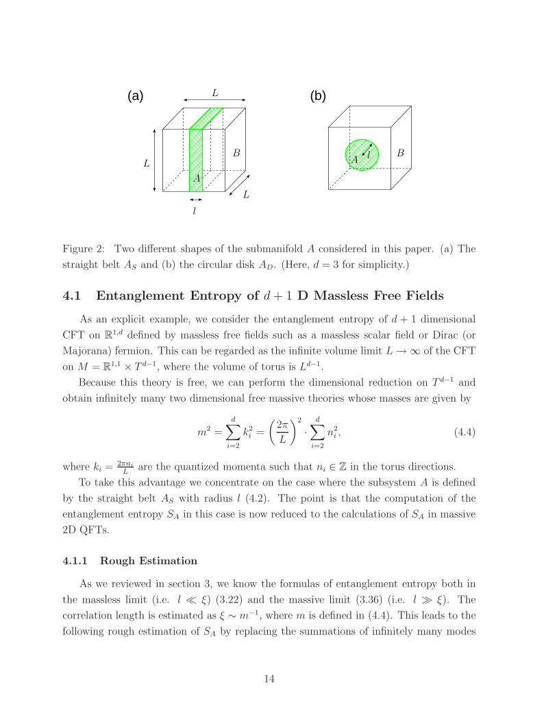
The first one is the straight belt of width l

AS = xi|x1 ∈ [−l/2, l/2], x2,3,···,d ∈ [−∞,∞], (4.2)

as depicted in Fig. 2. Since the lengths in the directions of x2, x3, · · ·, xd are infinite, we

often put the regularized length L. Taking the limit l → ∞ and looking at the region

near x1 = −l/2, we obtain the subsystem ASL which covers a half infinite space of Rd.

The boundary in this case is given by the straight surface ∂ASL = Rd−1.

The second example is the circular disk AD of radius l defined by

AD = xi|r ≤ l, (4.3)

where r =√

∑di=1 x

2i (see Fig. 2.).

13

L

L

L

l

l

(a) (b)

A

B BA

Figure 2: Two different shapes of the submanifold A considered in this paper. (a) The

straight belt AS and (b) the circular disk AD. (Here, d = 3 for simplicity.)

4.1 Entanglement Entropy of d+ 1 D Massless Free Fields

As an explicit example, we consider the entanglement entropy of d + 1 dimensional

CFT on R1,d defined by massless free fields such as a massless scalar field or Dirac (or

Majorana) fermion. This can be regarded as the infinite volume limit L→ ∞ of the CFT

on M = R1,1 × T d−1, where the volume of torus is Ld−1.

Because this theory is free, we can perform the dimensional reduction on T d−1 and

obtain infinitely many two dimensional free massive theories whose masses are given by

m2 =

d∑

i=2

k2i =

(

2π

L

)2

·d∑

i=2

n2i , (4.4)

where ki = 2πni

Lare the quantized momenta such that ni ∈ Z in the torus directions.

To take this advantage we concentrate on the case where the subsystem A is defined

by the straight belt AS with radius l (4.2). The point is that the computation of the

entanglement entropy SA in this case is now reduced to the calculations of SA in massive

2D QFTs.

4.1.1 Rough Estimation

As we reviewed in section 3, we know the formulas of entanglement entropy both in

the massless limit (i.e. l ≪ ξ) (3.22) and the massive limit (3.36) (i.e. l ≫ ξ). The

correlation length is estimated as ξ ∼ m−1, where m is defined in (4.4). This leads to the

following rough estimation of SA by replacing the summations of infinitely many modes

14

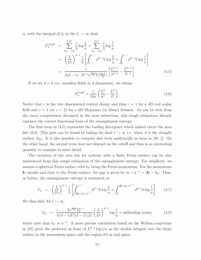
ni with the integral of ki in the L→ ∞ limit

SroughA =

ξ≤l∑

k2,··· ,kd

c

3log

ξ

a+

ξ≥l∑

k2,··· ,kd

c

3log

l

a

=

(

L

2π

)d−1c

3

[

∫ a−1

l−1

dd−1k logξ

a+

∫ l−1

0

dd−1k logl

a

]

=c

3(d− 1) · 2d−1πd−12 Γ(d+1

2)

[

Ld−1

ad−1− Ld−1

ld−1

]

. (4.5)

If we set d = 3 (i.e. massless fields in 4 dimension), we obtain

SroughA =

c

24π

(

L2

a2− L2

l2

)

. (4.6)

Notice that c is the two dimensional central charge and thus c = 1 for a 4D real scalar

field and c = 1 (or c = 2) for a 4D Majorana (or Dirac) fermion. As can be seen from

the exact computation discussed in the next subsection, this rough estimation already

captures the correct functional form of the entanglement entropy.

The first term in (4.5) represents the leading divergence which indeed obeys the area

law (2.8). This part can be found by taking the limit l → ∞ i.e. when A is the straight

surface ASL. It is also possible to compute this term analytically as done in [40, 2]. On

the other hand, the second term does not depend on the cutoff and thus is an interesting

quantity to examine in more detail.

The violation of the area law for systems with a finite Fermi surface can be also

understood from this rough estimation of the entanglement entropy. For simplicity, we

assume a spherical Fermi surface with kF being the Fermi momentum. For the momentum

k outside and close to the Fermi surface, the gap is given by m ∼ ξ−1 ∼ |k| − kF . Thus,

as before, the entanglement entropy is estimated as

SA =

(

L

2π

)d−1c

3

[

∫ a−1

|k|=kF +l−1

dd−1k logξ

a+

∫ |k|=kF +l−1

0

dd−1k logl

a

]

. (4.7)

We thus find, for l → ∞,

SA ∼ c

3

2πd−12 kd−1

F

(d− 1)Γ((d− 1)/2)

(

L

2π

)d−1

logl

a+ subleading terms, (4.8)

where note that kF ∝ a−1. A more precise calculation based on the Widom conjecture

in [31] gives the prefactor in front of Ld−1 log l/a as the double integral over the fermi

surface in the momentum space and the region ∂A in real space.

15

4.1.2 Exact Estimation from Entropic c-function

The previous approximation (4.5) uses the formulas which are exact only in the two

opposite limits ξ → ∞ and ξ → 0. To perform an exact estimation, we need to be

precise about the intermediate region ξ ∼ l. In other words, we need to use a sort of c-

function under the massive deformation corresponding to the interpolating region instead

of the UV central charge in (4.5). To make this more explicit we can employ the entropic

c-function C introduced in [42, 37, 39]. It is defined for 2D CFTs as follows

ldSA(l)

dl= C(lm), (4.9)

where l is the length of the subsystem A and m is the mass of the field. For massive free

fermions and scalar fields, the function C is characterized as a solution to a differential

equation of Painleve V type and its numerical form can be found in [37, 39]. Unfortunately,

its analytical expression is not known.

This function C(x) is positive and is also a monotonically decreasing function [42]

with respect to x as in the Zamolodchikov’s c-function [43]. These properties are indeed

true in explicit examples [39], which we reproduced in Fig. 3 for a free massive real scalar

boson and free Dirac fermion in 1+1 D. The function C(x) is normalized such that in the

UV limit x = 0 it is related to the ordinary central charge via C(0) = c/3. Note that if

we set C = C(0) = c/3, we recover from this equation the well-known result (3.22). We

will also show this later independently in (4.24). It was argued that the positivity of C(x)

is connected to a majorization relation for local density matrices [3, 4, 44, 45, 46]

In our example of the d+ 1 dimensional free field, we can reduce it to infinitely many

massive fields in two dimensions. Thus in this case we again just have to sum over the

discrete quantum numbers ni. In the limit L → ∞ we can replace the sum with an

integral

ldSA(l)

dl=

[

Ld−1

(2π)d−1

]∫

dk2 · · · dkd C(l|k|)

=

[

Ld−1

2d−2πd−12 Γ

(

d−12

)

]

∫ ∞

0

dkkd−2C(lk). (4.10)

The merit of the quantity C instead of SA itself is that it does not include UV divergences

16

and thus we can set a = 0 in C. After the integration of l we find

SA(l) =

[

Ld−1

2d−2πd−12 Γ

(

d−12

)

]

∫ ∞

0

dkkd−2

∫ l

a

dl

lC(lk),

=(

2d−1πd−12 Γ ((d+ 1)/2)

)−1

·[∫ ∞

0

dxxd−2C(x)

]

·[

Ld−1

ad−1− Ld−1

ld−1

]

≡ K

[

Ld−1

ad−1− Ld−1

ld−1

]

. (4.11)

where we determine the integral constant by requiring that SA(l) should be vanishing7

at l = a since we are cutting off degrees of freedom below the energy scale a−1. It is

straightforward to find analogous formula for the free massive fields. This is given just by

replacing k in (4.10) or (4.11) with√k2 +m2.

The second term in (4.11) does not depend on the cutoff a. Thus we are interested

in its coefficient K which is proportional to the integral of the function xd−2C(x). In

principle, we can compute it numerically based on the numerical results of C(x). Indeed

by this method the coefficient K was computed for three dimensional free fields in [39].

We extend it to four dimensions which we are interested in later discussions and present

the result as follows

K =

1

π

∫ ∞

0

dtC(t) ≃ 0.039, for d+ 1 = 3 dimensional real scalar boson

1

π

∫ ∞

0

dtC(t) ≃ 0.072, for d+ 1 = 3 dimensional Dirac fermion

1

4π

∫ ∞

0

dttC(t) ≃ 0.0049, for d+ 1 = 4 dimensional real scalar boson

1

4π

∫ ∞

0

dttC(t) ≃ 0.0097, for d+ 1 = 4 dimensional Majorana fermion.

(4.12)

To find the coefficient K in higher dimensions it is useful to notice that when x is large

the entropic c-function C(x) behaves as (Kν(x) is the deformed Bessel function)

Cscalar(x) ≃1

4xK1(2x), and CDirac(x) ≃

1

2xK1(2x), (4.13)

for a 2D free scalar field and a 2D Dirac fermion. When the dimension d is large, the

contribution of the integral∫

dxxd−2C(x) mainly comes from the large x region. Thus K

7It is possible that this requirement is not absolute, i.e. this choice of the cutoff a may depend on the

theory we consider. Thus only the constant K in front of the second term (i.e. finite term) in (4.11) has

a qualitative meaning.

17

0

0.05

0.1

0.15

0.2

0.25

0.3

0.35

0 0.5 1 1.5 2

C

t

free fermionfree boson

c=1/3

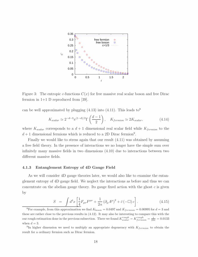
Figure 3: The entropic c-functions C(x) for free massive real scalar boson and free Dirac

fermion in 1+1 D reproduced from [39].

can be well approximated by plugging (4.13) into (4.11). This leads to8

Kscalar ≃ 2−d−3π(1−d)/2Γ

(

d− 1

2

)

, Kfermion ≃ 2Kscalar, (4.14)

where Kscalar corresponds to a d + 1 dimensional real scalar field while Kfermion to the

d+ 1 dimensional fermions which is reduced to a 2D Dirac fermion9.

Finally we would like to stress again that our result (4.11) was obtained by assuming

a free field theory. In the presence of interactions we no longer have the simple sum over

infinitely many massive fields in two dimensions (4.10) due to interactions between two

different massive fields.

4.1.3 Entanglement Entropy of 4D Gauge Field

As we will consider 4D gauge theories later, we would also like to examine the entan-

glement entropy of 4D gauge field. We neglect the interactions as before and thus we can

concentrate on the abelian gauge theory. Its gauge fixed action with the ghost c is given

by

S =

∫

d4x

[

1

4FµνF

µν +1

2α(∂µA

µ)2 + c (−) c

]

. (4.15)

8For example, from this approximation we find Kboson = 0.0497 and Kfermion = 0.00995 for d = 3 and

these are rather close to the previous results in (4.12). It may also be interesting to compare this with the

our rough estimation done in the previous subsection. There we found Kroughscalar = Krough

fermion = 124π = 0.0133

when d = 3.9In higher dimension we need to multiply an appropriate degeneracy with Kfermion to obtain the

result for a ordinary fermion such as Dirac fermion.

18

In order to compute the entanglement entropy, we consider the gauge theory on an n-

sheeted manifold Mn as before. We can rewrite the gauge field action as follows (we fix

the gauge by setting α = 1)

SAµ =

∫

d4x

[

1

4FµνF

µν +1

2(∂µA

µ)2

]

=

∫

d4x1

2∂µA

ν∂µAν +

[∫

d3x[−(∂νAν)A0 + (∂µA

0)Aµ]

]

surf

, (4.16)

where [· · ·]surf denotes the surface term when we performed an partial integration. If we

neglect the surface term, the theory is equivalent to four real scalar fields and a ghost

field which is a complex scalar. Since the complex ghost scalar field cancels two real

scalars, the theory is equivalent to two real scalar fields. However, there is a subtle issue

on the surface term that appears when we do the partial integration. Since fields are

discontinuous along the time direction in some region of the spacetime, we got surface

contributions. In this paper we assume such a term is not relevant for the computation

of the entanglement entropy as10 in [40].

4.2 Entanglement Entropy and Central Charges in 4D CFT

As we have seen, the entanglement entropy in 2D CFTs is proportional to the central

charge c. Since the central charge roughly measures the number of degrees of freedom

Ndof , we find the entanglement entropy is also proportional to Ndof . This fact is very

natural as its name of ‘entropy’ shows. Therefore we may expect that a similar story

is true also in the higher dimensional theories. As such an example, below we consider

4D CFTs. Indeed we will find that an important part of the entanglement entropy is

proportional to the central charges. See also [47, 41] for an earlier discussion.

In principle, it is possible to extend the relation between central charges and entan-

glement entropy to higher dimensions as far as the spacetime dimension is even. When

we consider odd dimensional spacetime, we do not have any clear definition of central

charges due to the absence of the Weyl anomaly. Under this situation, the entanglement

entropy may play an important alternative role 11.

10Indeed if we include such a contribution we find the total entropy of the gauge field becomes negative

in the particular case discussed in [40], which looks strange if we remember the original definition (2.3).11We are grateful to Anton Kapustin for pointing out this possibility to us.

19

4.2.1 Entanglement Entropy from Weyl Anomaly

Central charges in CFTs can be defined from the Weyl anomaly (or conformal anomaly)

〈T µµ 〉. Define the energy-momentum tensor T µν in terms of the functional derivative of

the (quantum corrected) action S with respect to the metric gµν

T µν =4π√g

δS

δgµν. (4.17)

In 2D CFTs, the Weyl anomaly is given by the well-known formula

〈T µµ 〉 = − c

12R, (4.18)

where R is the scalar curvature. We can regard this as a definition of the central charge

c in 2D CFTs.

Now we move on to 4D CFTs. In our normalization of (4.17), the Weyl anomaly can

be written as

〈T αα 〉 = − c

8πWµνρσW

µνρσ +a

8πRµνρσR

µνρσ. (4.19)

in a curved metric background gµν , where W and R are the Weyl tensor and the dual of

the curvature tensor. Notice that the second term is the Euler density. In terms of the

ordinary curvature tensor, we can express the curvature square terms in (4.19) as follows

WµνρσWµνρσ = RµνρσR

µνρσ − 2RµνRµν +

1

3R2,

RµνρσRµνρσ = RµνρσR

µνρσ − 4RµνRµν +R2. (4.20)

The coefficients c and a in (4.19) are called12 the central charges of 4D CFTs [48, 49,

50]. This is the original definition of the central charges in 4D CFTs. The central charge

a is believed to decrease monotonically under the renormalization group (RG) flow, while

for c this is not true and indeed counter examples are known; these properties of the

central charges a and c are confirmed in many supersymmetric examples e.g. [50].

To compute the entanglement entropy, we first consider the partition function Zn on

the d + 1 dimensional n-sheeted manifold Mn. Then we find the trace of ρn reduced to

the subsystem A is given by the formula (4.1). The entanglement entropy can be found

by taking the derivative of n with the n → 1 limit. If we define the length scale of the

manifold A by l, then the scaling of l is related to the Weyl scaling. They should be the

12The central charge a should not be confused with a UV cutoff. To avoid confusion, acutoff is used

to denote the UV cutoff in this subsection.

20

same13 at least in the n→ 1 limit. In this way we find

ld

dllog[trA ρ

nA] = 2

∫

dd+1x gµν(x)δ

δgµν(x)[logZn − n logZ1]

= − 1

2π

⟨∫

dd+1x√gT µ

µ (x)

⟩

Mn

+n

2π

⟨∫

dd+1x√gT µ

µ (x)

⟩

M1

.(4.21)

When we consider a CFT on M = Rd+1, the second term (i.e. integral on M1 = M =

Rd+1) become obviously vanishing. Below we omit writing the second term explicitly just

to make the appearance of expressions simple even if M is a curved manifold. Then the

entanglement entropy satisfies

ld

dlSA = − lim

n→1ld

dl

(

∂

∂nlog[trA ρ

nA]

)

=1

2πlimn→1

∂

∂n

⟨∫

dd+1x√gT µ

µ (x)

⟩

Mn

. (4.22)

4.2.2 Entanglement Entropy and Central Charges

Eq. (4.22) can be used to relate the entanglement entropy and central charge in a

direct fashion. Let us apply (4.22) to 2D CFTs first. We assume the submanifold A

is a segment of the length l in the total system. Then, the n-sheeted manifold Mn has

two conical singularities at u and v that separate A and B. If one goes around these

singularities, one picks up 2πn phase, i.e., 2π(n− 1) extra phase compared with 2π. (See

Fig. 1.) These singularities are reflected in the Euler number

χ[Mn] =1

4π

∫

Mn

d2x√gR = 2(1 − n), (4.23)

where we noted the scalar curvature is given by R = 4π(1 − n)[δ(2)(u) + δ(2)(v)] in the

presence of a deficit angle 2π(1 − n) at the conical singularities. Plugging (4.18) into

(4.22), we obtain

ld

dlSA = − ∂

∂n

(

c

24π

∫

d2x√gR

)

=c

3. (4.24)

We thus reproduce the known result (3.22) (see also (4.9)).

It is also possible to derive (3.36) from (4.22) by noting that

m∂SA

∂m= l

∂SA

∂l=

1

2πlimn→1

∂

∂n

⟨∫

d2x√gT µ

µ

⟩

. (4.25)

13Equally we can say that the scaling of l is oppositely related to the scaling of the cutoff i.e. l ddl =

−acutoff · ddacutoff

21

When A = ASL (i.e., A = 1 in (3.36) ), the integral on the right hand side is evaluated as

∫

d2x√g⟨

T µµ

⟩

= −π c6

(

n− 1

n

)

, (4.26)

by an argument similar to Zamolodchikov’s c-theorem [2]. We thus recover (3.36).

If we repeat the same analysis in 4D CFTs, we find

ld

dlSA = lim

n→1

∂

∂n

[

− c

16π2

∫

Mn

d4x√gWµνρσW

µνρσ +a

16π2

∫

Mn

d4x√gRµνρσR

µνρσ

]

(4.27)

= γ1 ·Area(∂A)

a2cutoff

+ γ2, (4.28)

where γ1 and γ2 are numerical constants. The first term in (4.28) comes from the integral

of the W 2 term in (4.27) and represents the leading divergence ∼ a−2cutoff . This is because

the curvature tensor is divergent as R ∼ a−2cutoff at the surface ∂A, where the deficit angle

presents and behaves like a delta function supported on ∂A. The Euler density term

does not have such a divergence since it is a topological invariant. Thus the constant

γ1 is proportional to c. Another constant γ2 comes from both terms in (4.27) and it is

proportional to the linear combination of a and c. By integrating (4.28), we can express

the entanglement entropy as follows

SA =γ1

2· Area(∂A)

a2cutoff

+ γ2 logl

acutoff+ Sothers

A , (4.29)

where the final term SothersA expresses terms which are independent of the total scaling

l → eαl. In other words, SothersA depends on the detailed shape of the surface ∂A. In this

way, the central charges determine the entanglement entropy up to these contributions

SothersA . Notice that the leading divergence (4.29) agrees with the area law (2.8). In our

later arguments using AdS/CFT duality, the gravity computations in section 7 reproduce

the same behavior as (4.29). When we assume a = c, both γ1 and γ2 are proportional to

a. This also agrees with our later gravity computations in section 7.3. For example, in

the N = 4 SU(N) super Yang-Mills the central charges are given by a = c = (N2 − 1)/4

[51] and thus they satisfy the condition.

In particular, when A is the circular disk AD with radius l, the system only depends

on l and acutoff . Thus the trace anomaly completely determines the entanglement entropy

SA. On the other hand, in the case of the straight belt AS there are two length scales

l and L and the result (4.29) becomes less predictive. Indeed the finite term which we

discussed before takes the form ∝ L2

l2and thus it is included in Sothers

A in (4.29). Since

this term is not directly related to the central charges, we expect that its value may be

22

shifted when we change the t’ Hooft coupling as is so in the thermal entropy. Indeed,

the comparison of the numerical results from the AdS5× S5 and the free N = 4 super

Yang-Mills supports this speculation as we will see in section 7.3.

Even though the constant γ1 is not universal in the sense that it depends on the choice

of the UV cut off, the other one γ2 is universal and an interesting quantity to evaluate.

In principle, this is reduced to a differential geometric computation. Since the evaluation

of total expression turns out to be rather complicated, below we would like to compute

some particular important terms.

It is straightforward to evaluate the contribution from the second term (Euler density)

in (4.27) because this is a topological term. As shown in [52], in a 4D manifold Mn with

a codimension two surface Σ around which conical singularities develop (with a deficit

angle 2π(1 − n)) we obtain

χ[Mn] =1

32π2

∫

Mn

d4x√gRR = (1 − n)χ[Σ] +

1

32π2

∫

Mn−Σ

d4x√gRR, (4.30)

where Mn − Σ denotes the smooth manifold defined by subtracting the singular part Σ

from Mn. Therefore the contribution of the R2 term in (4.27) to the constant γ2 is given

by

γtop2 = −2a · χ[∂A], (especially, γtop

2 = −4a when ∂A = S2). (4.31)

To make the analysis of the W 2 term in (4.27) simple, below we only consider the case

where the second fundamental form (or the extrinstic curvature) of ∂A, when embedded

in the 4D manifold Mn, can be neglected. This is true when we consider the straight

belt AS. Another typical example is when Mn is an Euclidean black hole and ∂A is its

horizon. We also concentrate on the case where ∂A is a connected manifold. Under these

assumptions we can employ the differential geometric results in [52]

∫

Mn

d4x√gR2−

∫

Mn−Σ

d4x√gR2 = 8π(1 − n)

∫

(RΣ + 2Rii −Rijij) + O((1 − n)2),

∫

Mn

d4x√gRµνρσRµνρσ−

∫

Mn−Σ

d4x√gRµνρσRµνρσ = 8π(1 − n)

∫

Rijij + O((1 − n)2),

∫

Mn

d4x√gRµνRµν−

∫

Mn−Σ

d4x√gRµνRµν = 4π(1 − n)

∫

Rii + O((1 − n)2), (4.32)

where RΣ is the intrinsic curvature of the 2D submanifold Σ; Rij and Rijkl denote the

curvature tensors projected onto the direction normal to Σ (e.g. Rij = Rµνnµi n

νj using the

two orthonormal vectors niµ (i = 1, 2) orthogonal to Σ). In the end, we obtain14 (this

14Refer also to [53] for an earlier computation of a similar expression of the logarithmic term from a

different approach.

23

includes both contributions from W 2 and R2)

γ2 =c

6π

∫

Σ=∂A

d2x√g (RΣ=∂A + 2Rijij − Rii) −

a

2π

∫

Σ=∂A

d2x√gRΣ=∂A. (4.33)

Especially when a = c,

γ2 = − a

6π

∫

Σ=∂A

d2x√g (2RΣ=∂A − 2Rijij +Rii) . (4.34)

under the previous assumption that the second fundamental form is zero. We will later

compare this result with the one from gravity side in section 7.3.

5 Holographic Interpretation

The main purpose of this paper is to compute the entanglement entropy in d + 1

dimensional conformal field theories CFTd+1 via the AdS/CFT correspondence. This

duality relates the CFTd+1 to the d+ 2 dimensional AdS space AdSd+2. Then we expect

that the entanglement entropy can be computed as a geometrical quantity in the AdSd+2

space just as the thermal entropy of CFTs is found from the area formula of AdS black

hole entropy [54].

As in section 3 the CFTd+1 is defined on M = R×N and we divide N into two regions

A and B. We assume the space-like d dimensional manifold N is now given by Rd or Sd

such that M is the boundary of AdSd+1 in the Poincare coordinates

ds2 = R2 dz2 − dx2

0 +∑d−1

i=1 dx2i

z2, (5.1)

or the global coordinates

ds2 = R2(

− cosh2 ρdt2 + dρ2 + sinh ρ2dΩ2d

)

, (5.2)

respectively.

5.1 General Proposal

In this setup we propose that the entanglement entropy SA in CFTd+1 can be computed

from the following area law relation

SA =Area(γA)

4G(d+2)N

. (5.3)

24

The manifold γA is the d-dimensional static minimal surface in AdSd+2 whose boundary is

given by ∂A. Its area is denoted by Area(γA). Also G(d+2)N is the d+2 dimensional Newton

constant. It is obvious that the leading divergence ∼ a−(d−1) in (5.3) is proportional to

the area of the boundary ∂A and this agrees with the known property (2.8).

This proposal is motivated by the following physical interpretation. Since the entan-

glement entropy SA is defined by smearing out the region B, the entropy is considered

to be the one for an observer in A who is not accessible to B. The smearing process

produces the fuzziness for the observer and that should be measured15 by SA. In the

higher dimensional perspective of the AdS space, such an fussiness appears by hiding a

part of the bulk space AdSd+2 inside an imaginary horizon, which we call γ. It is clear

that γ covers the smeared region B from the inside of the AdS space and thus we find

∂γ = ∂B(= ∂A). We expect that it is the holographic screen for the hidden part in the

bulk. To choose the minimal surface as in (5.3) means that we are seeking the severest

entropy bound [10, 11, 12] for the lost information. In the examples of AdS3/CFT2, we

will show below that the bound is actually saturated. Therefore it is natural to expect

that the bound is always saturated even in the higher dimensional (d ≥ 2) cases. These

considerations lead to our proposal (5.3). Notice also that the properties (2.4) and (2.5)

are obviously satisfied for (5.3).

It is also straightforward to extend this formula (5.3) to any asymptotically AdS spaces

and we argue that the claim remains the same in these generalized cases. For example,

if we consider a AdS Schwarzschild black hole, then the minimal surface γA wraps the

part of its real horizon as we will see later in section 7.5. This consideration fixes the

normalization of (5.3).

5.2 Intuitive Derivation from AdS/CFT

Let us try to understand how the area law (5.3) can be derived from known facts on

AdS/CFT correspondence. As we have seen in section 3, it is essential to compute trA ρnA

in order to obtain the entanglement entropy. It is equivalent to the partition function of

the CFT on the multiple (i.e. n times) covered space. Then SA can be found from the

formula (3.11).

Let us start with the AdS3/CFT2 example with a single interval. In this case as we

have seen, trA ρnA is equivalent to the n products of the two point functions 〈Φ+(k)

n Φ−(k)n 〉 as

in (3.17). The conformal dimension of Φ(k)±n is given by ∆n = c

24(1− n−2). The CFTs on

15It may be interesting to note that this origin of entropy is somewhat analogous to the recently

proposed ‘fuzzball’ picture (for a review see [55]).

25

disconnected n sheets (remember the description explained in section 3) is equivalent to

a CFT on a single sheet R2 whose central charge is nc with two twisted vertex operators

Φ+n and Φ−

n (distinguish them from Φ(k)±n ) inserted.

In AdS/CFT16, such a two point function 〈Φ+n (P )Φ−

n (Q)〉 in the CFT can be computed

as

〈Φ+n (P )Φ−

n (Q)〉 ∼ e−2n∆n·LPQ

R , (5.4)

where LPQ is the geodesic distance between P and Q. Therefore we can derive explicitly

the area law (5.3) as follows

SA = 2

(

∂(n∆n)

∂n

∣

∣

∣

∣

n=1

)

· LγA

R=

LγA

4G(3)N

, (5.5)

from AdS/CFT correspondence.

In higher dimensions, we can again compute trA ρnA as the path-integral over the multi

covered space with n sheets. We expect that this system is equivalent to a CFT on R1,d

which has the n replica fields φi(xµ) with a twist-like operator Φn inserted (assuming the

simplest case that ∂A is a connected manifold). Notice that this operator is localized in

codimension two subspace of R1,d. Then trA ρnA is equal to the one point function 〈Φn〉.

As in the Wilson loop operator case [64], we naturally expect that it can be computed as

〈Φn〉 ∼ e−αnAreaA, (5.6)

where AreaA is the area of the minimal surface in AdSd+2 whose boundary is ∂A; αn is a

n-dependent constant (limn→∞αn

n=finite).

This form (5.6) is almost clear from the following argument. First we notice that

log〈Φn〉 should be equal to the factor 1

G(d+2)N

times a certain diffeomorphism invariant

quantity as is clear from the supergravity side. Then the latter should have the momentum

dimension −d. Only such a candidate is essentially the area term as in (5.6), assuming

that it is given by a local integral.

Applying the formula (3.11) we find

SA =

(

∂αn

∂n

∣

∣

∣

∣

n=1

)

· AreaA. (5.7)

The coefficient can be fixed by requiring that the entanglement entropy at a finite tem-

perature should be reduced to the thermal entropy (i.e. black hole entropy) when A is

the total space (see also later discussions in section 7 on this point). This leads to (5.3).

16Here we consider the AdS dual of the CFT with central charge nc. Finally we take the limit n → 1.

26

6 Entanglement Entropy in 2D CFT from AdS3

We start with the AdS3 (d = 1) in the global coordinates (5.2). According to AdS/CFT

correspondence [5], the gravitational theories on this space are dual to 1 + 1 dimensional

conformal field theories with the central charge [56]

c =3R

2G(3)N

, (6.1)

where G(3)N is the Newton constant in three dimensional gravity17.

6.1 AdS3 Space and UV Cutoff in Dual CFTs

At the boundary ρ = ∞ of the AdS3, the metric is divergent. To regulate relevant

physical quantities we need to put a cutoff ρ0 and restrict the space to the bounded region

ρ ≤ ρ0. This procedure corresponds to the ultra violet (UV) cutoff in the dual conformal

field theory [25, 57]. If we define the dimensionless UV cutoff δ (∝ length), then we find

the relation eρ0 ∼ δ−1. In the example of the previous section, δ should be identified with

eρ0 ∼ δ−1 = L/a. (6.2)

Remember that L is the total length of the system and a is the lattice spacing (or UV

cutoff). Notice that there is actually an ambiguity about the O(1) numerical coefficient

in this relation18.

The holographic principle tells us that true physical degrees of freedom of the grav-

itational theory in some region is represented by its boundary of that region. This is

well-known in the black hole geometries and it leads to the celebrated area law of the

Bekenstein-Hawking entropy. In the context of AdS/CFT correspondence degrees of free-

dom in AdSd+1 space are represented by its boundary of the form Rt× Sd−1, where the

dual conformal field theory lives. We can compute the number of degrees of freedom Ndof

by applying the area law in three dimensional spacetimes to the boundary in the AdS3

space [57] . This leads to the following estimation

Ndof ∼ Boundary Length

4G(3)N

=2πR sinh ρ0

4G(3)N

≃ πc

6· La. (6.3)

17Remember that G(d+2)N is defined such as Sgravity = 1

16πG(d+2)N

∫

dd+2x√

gR+ .... for any dimension d.

18However, this ambiguity does not affect universal quantities which do not depend on the cut off a

and we will consider such quantities in the later arguments.

27

The central charge c is roughly proportional to the number of fields. The ratio L/a counts

the number of independent points in the presence of the lattice spacing a. Therefore the

result (6.3) agrees with what we expect from the conformal field theory at least up to the

unknown numerical coefficient.

6.2 Geodesics in AdS3 and Entanglement Entropy in CFT2

In the global coordinate of AdS3 (5.2), the 1 + 1 dimensional spacetime, in which the

CFT2 is defined, is identified with the cylinder (t, θ(≡ Ω1)) at the (regularized) boundary

ρ = ρ0. Then we consider the AdS dual of the setup in section 3.3. The subsystem A

corresponds to 0 ≤ θ ≤ 2πl/L and we can discuss the entanglement entropy by applying

our proposal (5.3). In this lowest dimensional example, the minimal surface γA, which

plays the role of the holographic screen [10, 11, 12], becomes one dimensional. In other

words, it is the geodesic line which connects the two boundary points at θ = 0 and

θ = 2πl/L with t fixed (see Fig. 4) .

Then to find the entropy we calculate the length of the geodesic line γA. The geodesics

in AdSd+2 spaces are given by the intersections of two dimensional hyperplanes and the

AdSd+2 in the ambient R2,d+1 space such that the normal vector at the points in the

intersections is included in the planes. The explicit form of the geodesic in AdS3, expressed

in the ambient ~X ∈ R2,2 space, is

~X =R√α2 − 1

sinh(λ/R) · ~x+R

[

cosh(λ/R) − α√α2 − 1

sinh(λ/R)

]

· ~y, (6.4)

where α = 1 + 2 sinh2 ρ0 sin2(πl/L); x and y are defined by

~x = (cosh ρ0 cos t, cosh ρ0 sin t, sinh ρ0, 0),

~y = (cosh ρ0 cos t, cosh ρ0 sin t, sinh ρ0 cos(2πl/L), sinh ρ0 sin(2πl/L)) . (6.5)

The length of the geodesic can be found as

Length =

∫

ds =

∫

dλ = λ∗, (6.6)

where λ∗ is defined by

cosh(λ∗/R) = 1 + 2 sinh2 ρ0 sin2 πl

L. (6.7)

Assuming that the UV cutoff energy is large eρ0 ≫ 1, we can obtain the entropy (5.3) as

follows (using (6.1))

SA ≃ R

4G(3)N

log

(

e2ρ0 sin2 πl

L

)

=c

3log

(

eρ0 sinπl

L

)

. (6.8)

28

t

θ

2πl/L

B

AγA ρ

(a)

B

A

γA

(b)

Figure 4: (a) AdS3 space and CFT2 living on its boundary and (b) a geodesics γA as a

holographic screen.

Indeed, this entropy exactly coincides with the known 2D CFT result (3.30), including

the (universal) coefficients after we remember the relation (6.2).

6.3 Calculations in Poincare Coordinates

It is useful to repeat the similar analysis in the Poincare coordinates (5.1). We pickup

the spacial region (again call A) −l/2 ≤ x ≤ l/2 and consider its entanglement entropy

as in section 3.2. We can find the geodesic line γA between x = −l/2 and x = l/2 for a

fixed time t0 (see also later analysis in section 7)

(x, z) =l

2(cos s, sin s), (ǫ ≤ s ≤ π − ǫ). (6.9)

The infinitesimal ǫ is the UV cutoff and leads to the cutoff zUV as zUV = lǫ2. Since

eρ ∼ xi/z near the boundary, we find z ∼ a. The length of γA can be found as

Length(γA) = 2R

∫ π/2

ǫ

ds

sin s= −2R log(ǫ/2) = 2R log

l

a. (6.10)

Finally the entropy can be obtained as follows

SA =Length(γA)

4G(3)N

=c

3log

l

a. (6.11)

This again agrees with the well-known result (3.22) as expected.

6.4 Entropy on Multiple Disjoint Intervals

Next we proceed to more complicated examples. Assume that the system A consists

of multiple disjoint intervals. The entanglement entropy can be computed as in (3.29).

29

In the dual AdS3 description, the region A corresponds to θ ∈ ∪Ni=1[

2πri

L, 2πsi

L] at the

boundary. In this case it is not straightforward to speculate the holographic screen (or

minimal surface) γA . However, the result in the 1+ 1 dimensional conformal field theory

(3.29) can be rewritten into the following simple form

SA =1

4G(3)N

[

∑

i,j

Length(rj , si) −∑

i<j

Length(rj , ri) −∑

i<j

Length(sj, si)

]

, (6.12)

where Length(A,B) denotes the length of the geodesic line between two boundary points

A and B. This shows how we choose γA. It is a linear combination of geodesic lines.

Their coefficients are either 1 or −1. Thus some of the coefficients turn out to be negative19. It is easy to see such negative coefficients are necessary by considering the limit where

si coincides with ri+1 and requiring it reproduces the result for N − 1 intervals.

6.5 Finite Temperature Cases

Next we consider how to explain the entanglement entropy (3.34) at finite tempera-

ture T = β−1 from the viewpoint of AdS/CFT correspondence. Since we assumed that

the spacial length of the total system L is infinite, we have β/L ≪ 1. In such a high

temperature circumstance, the gravity dual of the conformal field theory is described by

the Euclidean BTZ black hole [59]. Its metric looks like

ds2 = (r2 − r2+)dτ 2 +

R2

r2 − r2+

dr2 + r2dϕ2. (6.13)

The Euclidean time is compactified as τ ∼ τ + 2πRr+

to obtain a smooth geometry. We also

impose the periodicity ϕ ∼ ϕ + 2π. By taking the boundary limit r → ∞, we find the

relation between the boundary CFT and the geometry (6.13)

β

L=

R

r+≪ 1. (6.14)

The subsystem for which we consider the entanglement entropy is given by 0 ≤ ϕ ≤2πl/L at the boundary. Then by extending our proposal (5.3) to asymptotically AdS

19One may think the presence of minus signs is confusing from the viewpoint of holographic screen.

Instead we would like to regard this as a singular (or just complicated) behavior which is typical only

in the lowest dimension. In higher dimensional cases, we do not seem to have such a problem when ∂A

is compact. Notice also that the total sum (6.12) is always positive. If we replace the surface γA with

D-branes or fundamental strings (remember the similarity to Wilson loops) , the minus sign is analogous

to ghost branes introduced recently in [58].

30

spaces, the entropy can be computed from the length of the space-like geodesic starting

from ϕ = 0 and ending to ϕ = 2πl/L at the boundary r = ∞ for a fixed time. To find the

geodesic line, it is useful to remember that the Euclidean BTZ black hole at temperature

T is equivalent to thermal AdS3 at temperature 1/T . This equivalence can be interpreted

as a modular transformation in the boundary CFT [60]. If we define the new coordinates

r = r+ cosh ρ, τ =R

r+θ, ϕ =

R

r+t, (6.15)

then the metric (6.13) indeed becomes the one in the Euclidean Poincare coordinates with

t replaced by it. Now the computation of the geodesic line is parallel with what we did

in section 6.2. We only need to replace sinh ρ and sin t with cosh ρ and sinh t. In the end

we find (6.6) with λ∗ is now given by

cosh

(

λ∗R

)

= 1 + 2 cosh2 ρ0 sinh2

(

πl

β

)

, (6.16)

where we took into account the UV cutoff eρ0 ∼ β/a. Then our area law (5.3) precisely

reproduces the known CFT result (3.34). We can extend these arguments to the multi

interval cases as in the zero temperature case. We again obtain the formula (6.12) from

the CFT result (3.33).

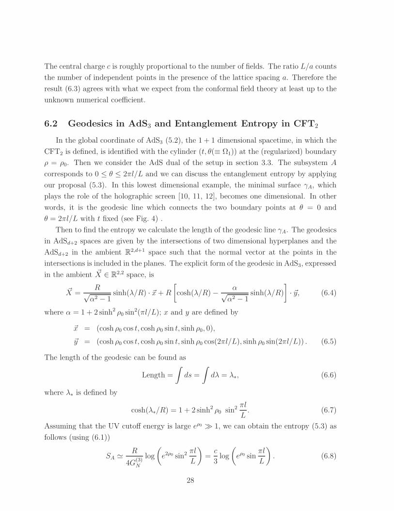
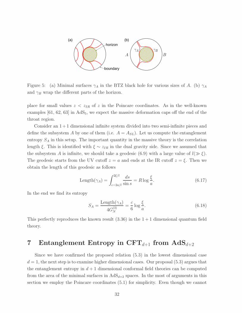
It is also useful to understand these calculations geometrically. The geodesic line in

the BTZ black hole takes the form shown in Fig. 5(a). When the size of A is small,

it is almost the same as the one in the ordinary AdS3. As the size becomes large, the

turning point approaches the horizon and eventually, the geodesic line covers a part of

the horizon. This is the reason why we find a thermal behavior of the entropy when

l/β ≫ 1 in (3.35). The thermal entropy in a conformal field theory is dual to the black

hole entropy in its gravity description via the AdS/CFT correspondence. In the presence

of a horizon, it is clear that SA is not equal to SB (remember B is the complement of A)

since the corresponding geodesic lines wrap different parts of the horizon (see Fig. 5(b)).

This is a typical property of entanglement entropy at finite temperature as we mentioned

in section 2.

6.6 Massive Deformation

Now we would like to turn to 1 + 1 dimensional massive quantum field theories. Such

a theory can be typically obtained by perturbing a conformal field theory by a relevant

perturbation. In the dual gravity side, this corresponds to a deformation of AdS3 space.

Since in the high energy limit the mass gap can be ignored, the deformation only takes

31

A

γA γB

B

(b)(a)horizon

boundary

Figure 5: (a) Minimal surfaces γA in the BTZ black hole for various sizes of A. (b) γA

and γB wrap the different parts of the horizon.

place for small values z < zIR of z in the Poincare coordinates. As in the well-known

examples [61, 62, 63] in AdS5, we expect the massive deformation caps off the end of the

throat region.

Consider an 1+1 dimensional infinite system divided into two semi-infinite pieces and

define the subsystem A by one of them (i.e. A = ASL). Let us compute the entanglement

entropy SA in this setup. The important quantity in the massive theory is the correlation

length ξ. This is identified with ξ ∼ zIR in the dual gravity side. Since we assumed that

the subsystem A is infinite, we should take a geodesic (6.9) with a large value of l(≫ ξ).

The geodesic starts from the UV cutoff z = a and ends at the IR cutoff z = ξ. Then we

obtain the length of this geodesic as follows

Length(γA) =

∫ 2ξ/l

ǫ=2a/l

ds

sin s= R log

ξ

a. (6.17)

In the end we find its entropy

SA =Length(γA)

4G(3)N

=c

6log

ξ

a. (6.18)

This perfectly reproduces the known result (3.36) in the 1 + 1 dimensional quantum field

theory.

7 Entanglement Entropy in CFTd+1 from AdSd+2

Since we have confirmed the proposed relation (5.3) in the lowest dimensional case

d = 1, the next step is to examine higher dimensional cases. Our proposal (5.3) argues that

the entanglement entropy in d+ 1 dimensional conformal field theories can be computed

from the area of the minimal surfaces in AdSd+2 spaces. In the most of arguments in this

section we employ the Poincare coordinates (5.1) for simplicity. Even though we cannot

32

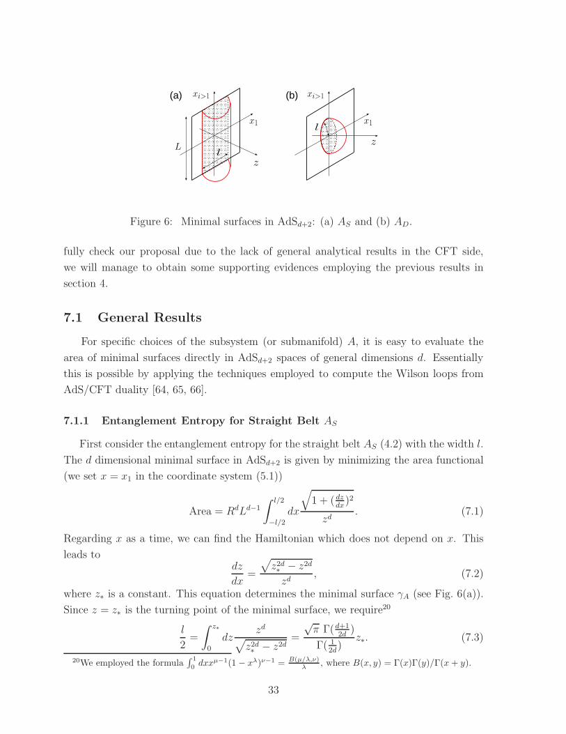
z

x1

z

x1

L

xi>1

l

(a) (b) xi>1

l

Figure 6: Minimal surfaces in AdSd+2: (a) AS and (b) AD.

fully check our proposal due to the lack of general analytical results in the CFT side,

we will manage to obtain some supporting evidences employing the previous results in

section 4.

7.1 General Results

For specific choices of the subsystem (or submanifold) A, it is easy to evaluate the

area of minimal surfaces directly in AdSd+2 spaces of general dimensions d. Essentially

this is possible by applying the techniques employed to compute the Wilson loops from

AdS/CFT duality [64, 65, 66].

7.1.1 Entanglement Entropy for Straight Belt AS

First consider the entanglement entropy for the straight belt AS (4.2) with the width l.

The d dimensional minimal surface in AdSd+2 is given by minimizing the area functional

(we set x = x1 in the coordinate system (5.1))

Area = RdLd−1

∫ l/2

−l/2

dx

√

1 + ( dzdx

)2

zd. (7.1)

Regarding x as a time, we can find the Hamiltonian which does not depend on x. This

leads todz

dx=

√

z2d∗ − z2d

zd, (7.2)

where z∗ is a constant. This equation determines the minimal surface γA (see Fig. 6(a)).

Since z = z∗ is the turning point of the minimal surface, we require20

l

2=

∫ z∗

0

dzzd

√

z2d∗ − z2d

=

√π Γ(d+1

2d)

Γ( 12d

)z∗. (7.3)

20We employed the formula∫ 1

0 dxxµ−1(1 − xλ)ν−1 = B(µ/λ,ν)λ , where B(x, y) = Γ(x)Γ(y)/Γ(x + y).

33

Then the area is given by

AreaAS=

2Rd

d− 1

(

L

a

)d−1

− 2IRd

(

L

z∗

)d−1

, (7.4)

where I is the constant

I =1

d− 1−∫ 1

0

dy

yd

(

1√

1 − y2d− 1

)

= −√π Γ(1−d

2d)

2d Γ( 12d

)> 0. (7.5)

In the end, we find the entanglement entropy from (5.3) using (7.3), (7.4) and (7.5)

SAS=

1

4G(d+2)N

2Rd

d− 1

(

L

a

)d−1

− 2dπd/2Rd

d− 1

(

Γ(d+12d

)

Γ( 12d

)

)d(

L

l

)d−1

, (7.6)

Notice that the first divergent term is proportional to the area of ∂A i.e. Ld−1 as we

expect from the known area law in the field theory computations (2.8). The second term

is finite and thus is universal (i.e. does not depend on the cutoff). This is the quantity

which we can directly compare with the field theory counterpart. Notice that our result

(7.6) does not include subleading divergent terms O(a−d+3). This is because AS is in the

straight shape. When we deform and bend it, the subleading divergent terms appear in

general as we will see later in another example. For example, in the 4D case, the absence

of log term is clear from the previous CFT analysis (4.34).

7.1.2 Entanglement Entropy for Circular Disk AD

Next we examine the case where subsystem A is given by the circular disk AD (radius l)

as defined in (4.3). We use the polar coordinate for Rd such that∑d

i=1 dx2i = dr2+r2dΩ2

d−1.

The minimum surface is the d dimensional ball Bd defined by z = z(r) (and Ωd−1 takes

arbitrary values). The function z(r) is found by minimizing the area functional

AreaAD= Rd · Vol(Sd−1) ·

∫ l

0

drrd−1

√

1 + (dzdr

)2

zd. (7.7)

We can find the following simple solution from the equation of motion21 for (7.7)

r2 + z2 = l2. (7.8)

21The equation of motion is given by rzz′′ + (d − 1)z(z′)3 + (d − 1)zz′ + dr(z′)2 + dr = 0.

34

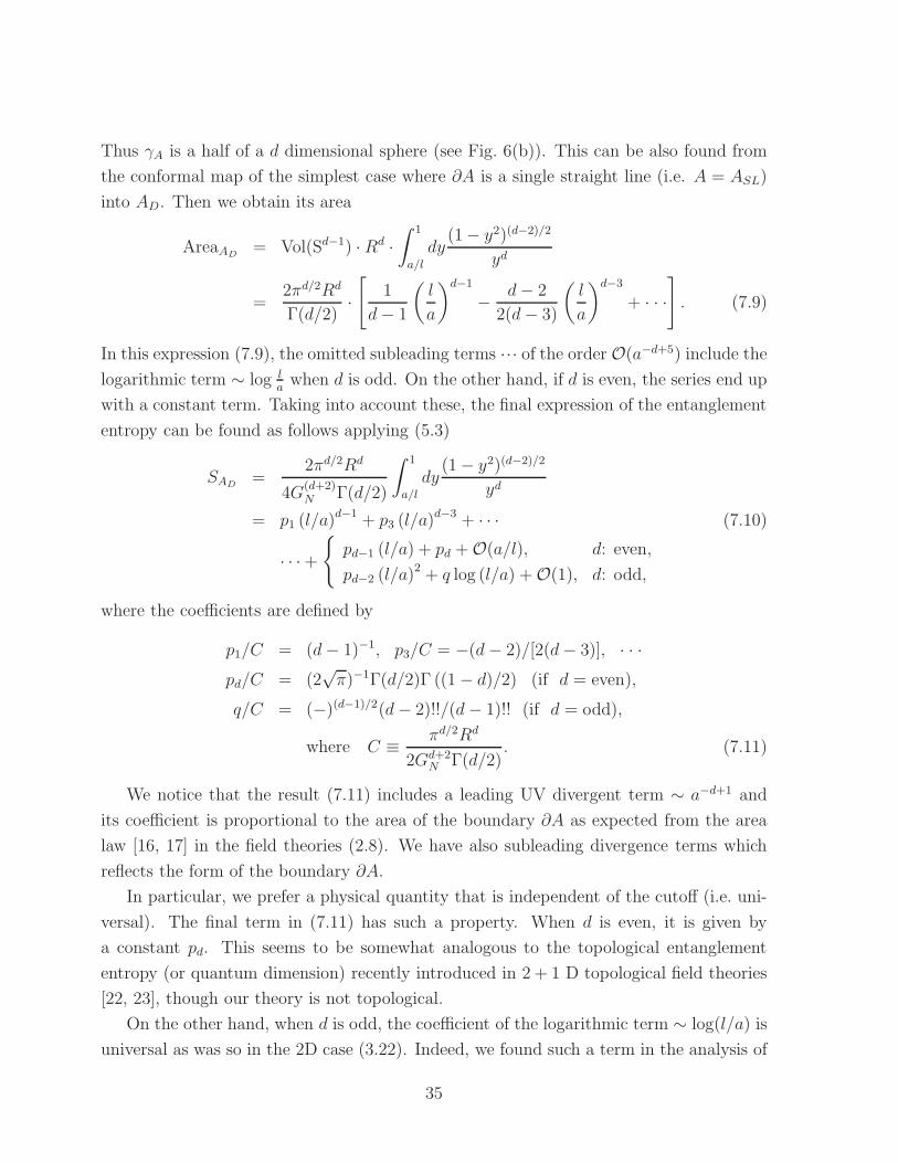
Thus γA is a half of a d dimensional sphere (see Fig. 6(b)). This can be also found from

the conformal map of the simplest case where ∂A is a single straight line (i.e. A = ASL)

into AD. Then we obtain its area

AreaAD= Vol(Sd−1) · Rd ·

∫ 1

a/l

dy(1− y2)(d−2)/2

yd

=2πd/2Rd

Γ(d/2)·[

1

d− 1

(

l

a

)d−1

− d− 2

2(d− 3)

(

l

a

)d−3

+ · · ·]

. (7.9)

In this expression (7.9), the omitted subleading terms ··· of the order O(a−d+5) include the

logarithmic term ∼ log la

when d is odd. On the other hand, if d is even, the series end up

with a constant term. Taking into account these, the final expression of the entanglement

entropy can be found as follows applying (5.3)

SAD=

2πd/2Rd

4G(d+2)N Γ(d/2)

∫ 1

a/l

dy(1 − y2)(d−2)/2

yd

= p1 (l/a)d−1 + p3 (l/a)d−3 + · · · (7.10)

· · · +

pd−1 (l/a) + pd + O(a/l), d: even,

pd−2 (l/a)2 + q log (l/a) + O(1), d: odd,

where the coefficients are defined by

p1/C = (d− 1)−1, p3/C = −(d− 2)/[2(d− 3)], · · ·pd/C = (2

√π)−1Γ(d/2)Γ ((1 − d)/2) (if d = even),

q/C = (−)(d−1)/2(d− 2)!!/(d− 1)!! (if d = odd),

where C ≡ πd/2Rd

2Gd+2N Γ(d/2)

. (7.11)

We notice that the result (7.11) includes a leading UV divergent term ∼ a−d+1 and

its coefficient is proportional to the area of the boundary ∂A as expected from the area

law [16, 17] in the field theories (2.8). We have also subleading divergence terms which

reflects the form of the boundary ∂A.

In particular, we prefer a physical quantity that is independent of the cutoff (i.e. uni-

versal). The final term in (7.11) has such a property. When d is even, it is given by

a constant pd. This seems to be somewhat analogous to the topological entanglement

entropy (or quantum dimension) recently introduced in 2 + 1 D topological field theories

[22, 23], though our theory is not topological.

On the other hand, when d is odd, the coefficient of the logarithmic term ∼ log(l/a) is

universal as was so in the 2D case (3.22). Indeed, we found such a term in the analysis of

35

4D conformal field theories e.g. (4.29), which is proportional to the central charge. This

issue will also be discussed in detail later.

This result is based on an explicit calculation when A = AD. However, from the paper

[66], we find that the behavior (7.10) is also true for any compact submanifold A with

different coefficient pk and q depending on the shape of A.

7.1.3 Multiple Loops

When the system A consists of M disconnected regions (we call them A1, A2, · · ·, AM ,

we need to find the minimal surface γA whose boundary ∂A is A1 ∪A2 ∪ · · · ∪AM . If the

distance between Ais are small enough we may find a connected surface of this property.

However, if they are far apart, γA can be separated into several pieces as pointed out by

[67] in the analogous problem of Wilson loop computations. Even if we take into account

this complexity, the inequality (subadditivity) S(A) ≤ S(A1) + S(A2) + · · · + S(AN) is

clearly satisfied.

It is also useful to consider a singular limit of such a multiple component case, i.e.

when the subsystem A consists of the multiple straight belts AS(1), AS(2), · · ·, AS(N). In

this situation, we can naturally obtain the entanglement entropy from the formula (6.12)

by replacing the geodesic distance with the area of the minimal surfaces. This agrees

with the free field computation which is a straightforward generalization of the result in

section 4.1.1.

7.2 Entanglement Entropy in N = 4 SYM from AdS5× S5

So far we have discussed low energy gravity theories on AdSd+2 and have not been

careful about its high energy completion as quantum gravity. To understand the holo-

graphic relation better including the various quantum corrections, it is necessary to re-

alize a concrete embedding into string theory. The most important such example is the

AdS5×S5 background in type IIB string theory. This background preserves the maximal

32 supersymmetries and is considered to be dual to the N = 4 SU(N) Super Yang-Mills

theory [5]. The supergravity approximation corresponds to the large t’ Hooft coupling

λ = Ng2Y M ≫ 1 (i.e. strongly coupled) region. The planar limit N → ∞ is equivalent to

the weakly coupled region gs → 0 of type IIB string. Since we perform the supergravity

analysis, the dual gauge theory is strongly coupled and the large N limit is taken.

The 5D Newton constant G(5)N is given in terms of the 10D one

G(10)N =

κ2

8π= 8π6α′4g2

s , (7.12)

36

as follows

G(5)N =

G(10)N

R5Vol(S5)=G

(10)N

π3R5. (7.13)

The radius R of AdS5 and S5 is expressed as

R = (4πgsα′2N)

14 . (7.14)

Plugging these values (7.13) and (7.14) into the previous results (7.6) and (7.10), we

obtain the following prediction of entanglement entropies in N = 4 SU(N) super Yang-

Mills theory

SAS=

N2L2

2πa2− 2

√π

(

Γ(

23

)

Γ(

16

)

)3N2L2

l2, (7.15)

SAD= N2

[

l2

a2− log

(

l

a

)

+ O(1)

]

. (7.16)

Notice that these are proportional to N2 as expected since the number of fields in the

SU(N) gauge theory is proportional to N2. Interestingly, (7.15) does not depend on

g2Y M = gs

2π.

Let us examine the first result (7.15). We notice that it has the same functional form

as in the free field theories (4.11). Since the second term in (7.15) is finite, it is interesting

to compare its coefficient with that of the free field theory result. The finite term in (7.15)

is numerically expressed as

SSugraAS

|finite ≃ −0.0510 · N2L2

l2. (7.17)

On the other hand, in the free field theory side we can employ the estimations (4.12). The

N = 4 super Yang-Mills consists of a gauge field Aµ, six real scalar fields (φ1, φ2, ···, φ6) and

four Majorana fermions (ψ1α, ψ

2α, ψ

3α, ψ

4α). As we explained in section 4.1.3, the contribution

from the gauge field is the same as those from two real scalar fields. In this way the total

entropy in the free Yang-Mills theory is the same as those from 8 real scalars and 4

Majorana fermions . Thus we obtain from (4.12) the following estimation

SFreeY MAS

|finite ≃ −(8 × 0.0049 + 4 × 0.0097) · N2L2

l2= −0.078 · N

2L2

l2. (7.18)

We observe that the free field result is larger than that in the gravity dual by a factor

∼ 32. This deviation is expected since the computation of the entanglement entropy22

22As we notice in section 4.2, some parts of entanglement entropy are proportional to the central

charges. They remain the same under exactly marginal deformation (e.g. changing coupling gY M) since

central charges do so.

37

includes non-BPS quantities due to the anti-periodic boundary condition of fermions

which appears when we compute the partition function on n−sheeted manifold Mn. This

situation is very similar to the computation of thermal entropy [54], where we have a

similar discrepancy (so-called 43

problem). The fact that the discrepancy is of order

one also in our computation can be thought as an encouraging evidence for our proposal.

Also notice that the coefficient in the free Yang-Mills is larger than the one in the strongly

coupled Yang-Mills. This is natural since the interaction of the form Tr[φi, φj]2 reduces

the degrees of freedom [6].

Next we turn to our second result (7.16). In addition to the area law divergence, it

includes a logarithmic term, whose coefficient is universal. This qualitative dependence

of the entropy (7.16) on l agrees with our previous result from the Weyl anomaly (4.29).

We will discuss the coefficient in front of the logarithmic term in more detail in the next

subsection.

7.3 Entanglement Entropy and Central Charges in 4D CFT

from AdS5

We can extend the previous computation to more general (i.e. less supersymmetric)

conformal backgrounds by replacing S5 with a compact five dimensional Einstein manifold

X5. The radius R of AdS5 and X5 is given by [68, 51]

R =

(

4π4gsα′2N

Vol(X5)

)14

, (7.19)

where N is again the number of D3-branes (or rank of the gauge group). The volume

Vol(X5) of X5 is known to be inversely proportional to the central charge a [51]. Note

that a = c always holds when a CFT has its gravity dual of the form AdS5 ×X5. In the

N = 4 SU(N) super Yang-Mills theory the central charge is given by aN=4 = N2−14

≃ N2

4.

The entanglement entropy SA in general 4D CFTs of this type is given in terms of

SN=4A in N = 4 SU(N) super Yang-Mills theory

SA =

(

a

aN=4

)

· SN=4A , (7.20)

i.e. SA is proportional to the central charge a. This is naturally understood by considering

that the central charge a measures degrees of freedom in the 4D CFT. Notice that here

we are assuming a strongly coupled 4D CFT in order to apply the AdS/CFT duality.

In our previous CFT analysis done in section 4.2, we have only shown that a part of

entanglement entropy is proportional to the central charge (4.29).

38

As we have seen, the coefficient of the logarithmic term (called γ2 in section 4.2) in

(7.16) is universal and is given by the central charge a times a numerical factor. Thus

it is very interesting to compare the factor between the gauge theory and the gravity.

When the 2D surface ∂A is generic (with a finite size) and the background is an arbitrary

asymptotically AdS5 space, the logarithmic term in the area of the minimal surface γA

can be found from the general formula given in [66]. This leads to

ldArea(∂A)

dl|finite =

∫

∂A

d2x√g

(

−1

8|H|2 − 1

4gαβRαβ +

1

12R

)

, (7.21)

where α and β are the coordinates which are tangent to ∂A and orthogonal to i, j direc-

tions; H is the mean curvature. As we did in section 4.2, we work below under the special

assumption that the second fundamental forms are zero to make arguments simple. Then

we can show

R ≃ RΣ=∂A + 2Rii −Rijij,

gαβRαβ ≃ RΣ=∂A +Rii −Rijij . (7.22)

We can also neglect |H|2 term in (7.21). In the end, we can rewrite (7.21) into the

following form

ldArea(∂A)

dl|finite =

∫

∂A

d2x√g

(

1

6Rijij −

1

12Rii −

1

6RΣ=∂A

)

. (7.23)

By considering the setup dual to the 4D N = 4 SU(N) super Yang-Mills theory (a = c ≃N2

4), it is straightforward to check that the gravity result (7.23) agrees23 with the previous

result (4.34) obtained from the Weyl anomaly24. It will be an interesting future problem

to examine terms which include the second fundamental forms and check the complete

agreement.

7.4 Entanglement Entropy from AdS4,7×S7,4 in M-theory

Other important supersymmetric examples of AdS spaces are AdS4×S7 and AdS7×S4

in eleven dimensional supergravity (or M-theory). They preserve the maximal 32 super-

symmetries. They are considered to be dual to 3D N = 8 SCFT and 6D (2, 0) SCFT,

23Under this assumption we cannot deal with the circular disk case AD because the second fundamental

forms are non-zero (i.e. Γiαβ 6= 0). However, it is possible to see that the contribution (4.31), which

comes from the topological term R2, coincides with the gravity result. Indeed we expect that the other

contribution from the Weyl tensor term W 2 is vanishing since the disk is conformally equivalent to the

straight line, in which case there is no log term (notice also that the W 2 term is a conformal invariant).24The derivation of the Weyl anomaly from the AdS/CFT duality was first done in [68].

39

respectively [5, 6]. They are obtained from the world-volume theories on M2 and M5-

branes (or strongly coupled limit of D2 and D4-branes). The numbers of the branes are

denoted by N . Since these theories have not been completely understood due to the

strongly coupled problem, it will be very useful to compute any new physical quantities.

The 11D Newton constant G(11)N is given in terms of 11D plank length lp as follows25

(2π)8l9p = 16πG(11)N = 2κ2

11. (7.24)

Let us first discuss the AdS4×S7 example. The radius of AdS4 and S7 are

2RAdS4 = RS7 = lp(32π2N)16 . (7.25)

The four dimensional Newton constant can be found after the compactification on S7

G(4)N =

48π3l9pR7

S7

. (7.26)

Then we find the following entanglement entropy defined for the straight belt AS

SAS=

Area

4G(4)N

=

√2

3N3/2

[

L

a− 4π3

Γ(1/4)4

L

l

]

. (7.27)

The entropy for the circular disk AD we find

SAD=

Area

4G(4)N

=

√2π

3N3/2

[

l

a− 1

]

. (7.28)

Notice that the constant terms in (7.27) and (7.28) are universal. The dependence ∼ N3/2

of degrees of freedom is typical in the 3D N = 8 SCFT.

In the AdS7× S4 case, in addition to (7.24), we have

RAdS7 = 2RS4 = 2lp(πN)13 , (7.29)

and

G(7)N =

6π5l9pR4

S4

. (7.30)

Then we find the following results

SAS=

2

3π2N3

[

L4

a4− 16π5/2

(

Γ(3/5)

Γ(1/10)

)5L4

l4

]

. (7.31)

SAD=

32

9N3

[

1

4· l

4

a4− 3

4· l

2

a2+

3

8log(l/a)

]

. (7.32)

Notice that the constant term in (7.31) and the coefficient of log(l/a) in (7.32) are uni-

versal. The overall dependence ∼ N3 is again peculiar to 6D (2, 0) SCFT.25Our convention is such that S11Dsugra = 1

2κ211

∫

d11x[√

gR + · · · ]. We follow the convention in [6].

40

7.5 Finite Temperature Case

Consider the N = 4 super Yang-Mills theory on R4 at finite temperature T . This

system is dual to the AdS black hole geometry [25, 69]

ds2 = R2

[

du2

hu2+ u2

(

−hdt2 + dx21 + dx2

2 + dx23

)

+ dΩ25

]

, (7.33)

where

h = 1 − u40

u4, u0 = πT. (7.34)

Various analyzes show that this theory has properties of a confining gauge theory [69, 6].

We would like to compute the entanglement entropy for the straight line in this

model. The subsystem A is defined by t = fixed, −l/2 ≤ x(≡ x1) ≤ l/2, u → ∞,

and x2, x3 =arbitrary. The regularized volume in the x2 and x3 direction is denoted by

L2. Then the area is given by26

Area = R3L2

∫ l/2

−l/2

dxu3

√

1 +u′2

u4 − u40

. (7.35)

We can integrate the equation of motion as

du

dx=√

(u4 − u40)(u

6/u6∗ − 1). (7.36)

We requirel

2=

∫ ∞

u∗

du1

√

(u4 − u40)(u

6/u6∗ − 1)

, (7.37)

where u∗(> u0) is the value of u(x) at the turning point x = 0. Using (7.36) we can

rewrite (7.35)

Area = 2R3L2

∫ ∞

u∗

duu6

√

(u4 − u40)(u

6 − u6∗). (7.38)

As usual, (7.38) contains the UV divergent term which is proportional to a−2. However,

we are interested in the term which is peculiar to this kind of confining gauge theory.

Indeed we can find that in the large l limit (i.e. u∗ ∼ u0), the main contribution (except

the UV divergence) of the integrals (7.37) and (7.38) comes from the region near u = u∗,

which leads to the relation

Areafinite ∼ π3N2R3L2lT 3. (7.39)

26This system is very similar to the one that appears in the computation of Wilson loop at finite

temperature [70].

41

Thus we obtain the finite part (i.e. we subtracted the UV divergent terms) of the entropy

in this limit

Sfinite =π2N2

2T 3L2l =

π2N2

2T 3 × Area(A). (7.40)

The important point is that this entropy (7.40) is proportional to the area of not ∂A

but A as opposed to the area law term (5.3). Thus it is extensive as in the thermal

entropy. This agrees with the field theory side since the entanglement entropy should

include the thermal entropy contribution as is obvious from its definition. In the gravity

side, it occurs because γA wraps a part of the black hole horizon and thus (7.40) is equal

to the fraction of black hole entropy, which shows the thermal behavior. This means

that the behavior of the entanglement entropy is rather different before and after the

cofiniment/de-confinement transition when we consider the N = 4 super Yang-Mills on

R×S3 (see [71] and references therein for recent studies of this phase transition). Thus the

entanglement entropy plays an role similar to an “order parameter”. Other geometrical

properties are also parallel with the AdS3 case as Fig. 5 shows.

7.6 Massive Deformations

As a final example we would like to discuss the entanglement entropy in d + 1 di-

mensional massive QFTs. Typically we can obtain such theories by considering massive

deformations of a d + 1 dimensional CFT. In principle, this can be done by looking at

supergravity solutions dual to non-conformal field theories such as [62, 61, 63]. Instead

here we approximate the geometry simply by cutting off the IR region z > ξ of the AdSd+2

space as we did in the d = 1 case. Here ξ is the correlation length and we are assuming

ξ ≫ l. 27

7.6.1 Straight Belt AS

Let us start with the computation of the entanglement entropy for the straight belt in

a massive theory by the simple method explained in the above. This leads to the following

27When a quantum ground state of a massive theory has non-trivial Berry phases, contribution from

the Berry phase to the entanglement entropy is also important [72].

42

estimation

SAS= 2

RdLd−1

4G(d+2)N

×∫ ξ

a

dz

√

(

dxdz

)2+ 1

zd=

Ld−1Rd

2G(d+2)N zd−1

∗

∫ ξ/z∗

a/z∗

dλ

λd√

1 − λ2d

=RdLd−1

2G(d+2)N

[

− a−d+1

−d + 1+

ξ−d+1

−d + 1

+1

2

1

d+ 1

ξd+1

z2d∗

+ · · ·+ (2n− 1)!!

(2n)!!

1

(2n− 1)d+ 1

ξ(2n−1)d+1

z2nd∗

+ · · ·]

=RdLd−1

2G(d+2)N

[

a−d+1

d− 1− ξ−d+1

d− 1+ r1

ξd+1

l2d+· · ·+ rn

ξ(2n−1)d+1

l2nd+· · ·

]

, (7.41)

where ris are some numerical constants. We assumed the same form of the minimal

surface as in the conformal case and thus the relation between z∗ and l is the same as

before (7.3).

7.6.2 Circular Disk AD

Next we examine the entanglement entropy for the circular disk AD (radius l) in a

massive theory. We assume the same minimal surface r2 + z2 = l2 as in the conformal

case.

SAD=

RdVol(Sd−1)

4G(d+2)N

∫

dr rd−1

√

1 + (dzdr

)2

zd

=2πd/2Rd

4Γ(d/2)G(d+2)N

∫ ξ/l

a/l

dy(1 − y2)

(d−2)/2

yd. (7.42)

43

The integral in the final expression in (7.42) has the following series expansion when d is

even (we set d = 2n)∫ ξ/l

a/l

dy(1 − y2)(d−2)/2

yd

=

[

− 1

d − 1

(

l

ξ

)d−1

+d− 2

2(d− 3)

(

l

ξ

)d−3

+ · · ·

· · · − (−1)n

2nn!

(d− 2n)(d− 2n+ 2) · · · (d− 2)

d− 2n− 1

(

l

ξ

)d−2n−1

+ · · ·]

+

[

1

d− 1

(

l

a

)d−1

− 1

2

d− 2

d− 3

(

l

a

)d−3

+ · · ·

· · · + (−1)n

2nn!

(d− 2n)(d− 2n+ 2) · · · (d− 2)

d− 2n− 1

(

l

a

)d−2n−1]

, (7.43)

where the expansion of a/l is truncated since we take the limit a→ 0 in the final expres-

sion.

When d is odd (d = 2n+ 1), we obtain the same result (7.43) except that we have to

be careful about the two terms O(

(l/ξ)d−2n−1)

and O(

(l/a)d−2n−1)

in (7.43) which are

proportional to 1d−2n−1

→ ∞. The divergences are canceled out and produce a log term

(−1)d−12

(d− 2)!!

(d− 1)!!log

ξ

a. (7.44)

Thus in the odd d case, we just have to replace the two terms in (7.43) with (7.44). Note

that this term has the same coefficient as the one in the conformal case, i.e. q/C in (7.11)

in our approximation. In summary we find

SAD=

2πd/2Rd

4Γ(d/2)G(d+2)N

[

1

d− 1

ld−1

ad−1+ (subleading divergences O(ld−3/ad−3))

]

+2πd/2Rd

4Γ(d/2)G(d+2)N

[

− 1

d− 1

ld−1

ξd−1+ O(ld−3/ξd−3)

]

+

0 d: even,

(−1)d−12

2πd/2(d− 2)!!Rd

4Γ(d/2)(d− 1)!!G(d+2)N

· logξ

ad: odd.

(7.45)

7.7 Entanglement Entropy in Some Non-Conformal Theories

The best way to derive the entanglement entropy in massive (or non-conformal) the-

ories is to start with their dual supergravity backgrounds instead of the previous crude

44

approximation. Since usually such backgrounds include complicated metric and many

other fields, we would like to make a first step by looking at some simple cases such

as the near horizon limit of Dp-branes. Here we would like to examine the example of

the D2-branes and NS5-branes. It will be an interesting future problem to analyze more

complicated but more realistic examples.

7.7.1 D2-branes Case

The decoupling limit of supergravity solution for N D2-branes is given by the following

metric and dilaton [73]

ds2 = α′(

U5/2

gY M

√6π2N

(−dx20 + dx2

1 + dx22) +

gY M

√6πN2

U5/2dU2 +

gY M

√6π2N

U1/2(dΩ6)

2

)

,

e2φ = g2Y M

(

gY M

√6π2N

U5/2

)1/2

. (7.46)

This supergravity background (7.46) is dual to the field theory limit of world-volume

theory on N D2-branes. This field theory is described by the 3D SU(N) super Yang-Mills

theory with the dimensionful coupling constant gY M(∝ energy1/2). The radial direction

U is proportional to the energy scale in this field theory.

To avoid the strongly coupled region gs ≫ 1 and the high curvature region α′R ≫ 1,

we trust the supergravity solution (7.46) when [73]

g2Y MN

1/5 ≪ U ≪ g2Y MN. (7.47)

The other two regions U ≫ g2Y MN

1/5 and U ≪ g2Y MN are well described by the 3D

superconformal field theory (or M2-branes) and the weakly coupled Yang-Mills theory,

respectively.

Under this condition (7.47), we would like to compute the entanglement entropy holo-

graphically in the straight belt case A = AS. First we notice that the dilaton is not

constant and thus the definition of G(4)N is not clear. However, it is easy to find a nat-

ural extension of our formula (5.3) by remembering the relation 1

G(4)N

= 1

G(10)N

∫

S6 d6x√g.

Consider the following functional for any 2D surface γA such that ∂γA = A

1

4G(10)N

∫

γA×S6

d8x e−2φ√g, (7.48)

and try to minimize it. This procedure singles out what should be called a minimal surface

γA. It is trivial to see that this procedure is reduced to the original relation (5.3) when

the dilaton is constant.

45

Then we find that γA is defined by (the notation is the same as in section 7.1.1)

dU

dx=

U5/2

gY M

√6π2N

√

U7

U7∗− 1, (7.49)

where U∗ is the turning point of the surface and we assume g2Y MN

1/5 ≪ U∗. Following

the same way of analysis in section 7.1, in the end we obtain the entanglement entropy

SAS=NLU2

0

5πg2Y M

− c · N5/3L

(gY M)2/3l4/3, (7.50)

where U0 is the UV cutoff (assuming U0 ≪ g2Y MN), and c = 1

5

(

4√

2√3

)4/3

π3/2(

Γ(5/7)Γ(3/14)

)7/3

.

The first term is proportional to the length of γA (i.e. L) in (7.50) and is an analogue

of the area law divergence term28. The second term is interesting since it is finite and

depends on l, non-trivially. Its N dependence ∝ N5/3 is between the free field result N2,

and the IR fixed point result N3/2 (see (7.27)) of the 3D N = 8 superconformal field

theory, as expected. As in the 4D case, we learn that the Yang-Mills interaction reduces

the degree of freedom.

7.7.2 NS5-branes Case

The throat part of N NS5-branes is described by the following well-known metric

[74, 73]

ds2 = −dx20 +

5∑

i=1

dx2i +Nα′dU

2

U2+Nα′(dΩ3)

2,

eφ =

(

(2π)3N

g2Y MU

2

)1/2

. (7.51)

We assume type IIB string theory to fix notations. To take the decoupling limit, we keep

the Yang-Mills coupling g2Y M = (2π)3α′ finite and take the limit gs → 0. This leads to

the little string theory (for a review see [75]). Notice that this theory is not a local field

theory and shows non-local behaviors such as the Hagedorn transition.

The calculation of the entanglement entropy can be done as before. However, in this

case29 of NS5-branes, we encounter the following unusual feature. Consider the straight

28It is proportional to the square of the cut off energy and is different from the area law relation (2.8).

However, this is not any contradiction because we cannot set U0 → ∞ due to the constraint (7.47). In

such a high energy region, we cannot neglect the stringy corrections and it is better to use the weakly

coupled Yang-Mills description.29Via the S-duality the analysis of the D5-branes leads to the same result.

46

line case and try to find solutions for the minimal surface equation

dU

dx=

√

(2π)3

Ng2Y M

U2

(

U4

U4∗− 1

)

. (7.52)

Smooth solutions are allowed only for a fixed value of l∗

l∗ =

∫ ∞

U∗

(

dx

dU

)

dU =

√

Ng2Y M

4√

2π=π

2

√Nα′. (7.53)

This suggests a phase transition at the energy scale (l∗)−1. Indeed, the value l−1 ∼ 1√Nα′

is the order of the Hagedorn temperature TH in the little string theory30. At least, we

can claim from the computation in (7.53) that there is no solution when l < l∗. We can

understand this because the lack of locality means that we cannot define the entanglement

entropy when the size of A becomes the same order of T−1H .

8 Conclusions and Discussions

In this paper we presented detailed discussions of the holographic interpretation of

the entanglement entropy proposed in our earlier letter [9]. We gave a derivation of our

proposal (5.3) in the AdS3/CFT2 case by applying the basic computation [24, 25] of

correlation functions in AdS/CFT correspondence. As for the higher dimensional case,

we are still lacking its complete derivation from standard AdS/CFT correspondence, even

though we offered an intuitive explanation and several non-trivial evidences of our proposal

(5.3). This deserves further investigations. The proof of the strong subadditivity (2.6)

will also be a non-trivial test for this purpose, say.

The application of the proposal (5.3) to various quantum field theories is also intrigu-

ing. Since we mainly analyzed the conformal field theories, it would be useful to compute

the entanglement entropy in massive theories. In this paper, we did a rough approximation

by cutting off the IR region by hand and also analyzed simple non-conformal backgrounds

of D2-branes and NS5-branes. The next step will be to compute the entanglement entropy

by considering supergravity backgrounds dual to more realistic massive theories such as

4D confining theories. There we expect that the entanglement entropy can be used as an

alternative of the Wilson loop to distinguish the confinement. Indeed, we already noticed

that the behavior of entanglement entropy is drastically changed before and after the

deconfinement phase transition in N = 4 super Yang-Mills theory at finite temperature

30The holographic entanglement entropy in this case takes the form of SAS= c1 · NL4

gY M2U2

0 −c2L4N2 U2

∗

l2 ,

where c1 and c2 are a certain constant.

47

from the AdS5 side. Also, we obtained a singular behavior of the entanglement entropy in

the background with many NS5-branes, which will probably be related to the non-locality

or the Hagedorn transition in the little string theory.

We also investigated the properties of the entanglement entropy from the conformal

field theory side. Especially we showed that important parts of entanglement entropy

are proportional to central charges in any 4D CFTs from the analysis of Weyl anomaly.

Even though we did not find this property for the other parts of the entropy, which

are invariant under the Weyl scaling, the holographic analysis tells us that the total

entanglement entropy in strongly coupled 4D CFTs is proportional to the central charge

a. These facts offer us an evidence that the central charge is proportional to degrees

of freedom in a given conformal field theory. It would be an interesting future problem

to study the relation between possible c-theorems in more than two dimensions and the

property of entanglement entropy.

Several aspects of the entanglement entropy revealed in this paper can have many

implications on (strongly interacting) QFTs, some of which might be realized in condensed

matter physics, say. For example, we derived the scaling of entanglement entropy (7.10)

for a compact submanifold A based on AdS/CFT correspondence where the coefficients pd

and q are universal and conformal invariant. We expect that this is a generic feature which

might be applicable for systems that does not necessarily have gravity (AdS) description.

Thus, it is interesting to investigate these quantities in several strongly interacting systems

at criticality. In a sense, these quantities are a generalization of the central charges

in CFTs in even spacetime dimensions, or the quantum dimension in topological field

theories. (Note also that there is no counter part of the central charges in odd spacetime

dimensions.) For example, at least in principle, we can numerically study these universal

quantities in the entanglement entropy in gapless spin liquids, and compare them with

those computed from several candidate effective field theories [18]. Also, even though these

effective field theories are suspected to be a gauge theory, it might not be straightforward

to identify the Wilson loop operator in a generic microscopic spin model. In that situation,

one can instead look at the entanglement entropy since our analysis for AdS black holes

suggests it can be at least as useful as the Wilson loop.

Finally, our computation of entanglement entropy may also be useful to uncover holo-

graphical duals of string theory backgrounds which are not well-understood, such as de-

Sitter spaces and Godel spaces31. This is because the entanglement entropy captures

the basic degrees of freedom in the dual theory and because it can be easily estimated

classically in the gravity side.

31Recent discussions on these spaces from this viewpoint can be found e.g. in [76] and [77].

48

Acknowledgments

We are very grateful to M. Einhorn, D. Fursaev, A. Kapustin, M. Levin, A. W. W.

Ludwig, T. Okuda, J. Preskill, and especially to H. Ooguri and M. Shigemori for useful

discussions and to R. Emparan for helpful correspondence. The work was supported in

part by the National Science Foundation under Grant No. PHY99-07949.

References

[1] C. Holzhey, F. Larsen and F. Wilczek, “Geometric and renormalized entropy inconformal field theory,” Nucl. Phys. B 424, 443 (1994) [arXiv:hep-th/9403108].

[2] P. Calabrese and J. Cardy, “Entanglement entropy and quantum field theory,” J.Stat. Mech. 0406, P002 (2004) [arXiv:hep-th/0405152]; “Entanglement entropy andquantum field theory: A non-technical introduction,” [arXiv:quant-ph/0505193].

[3] G. Vidal, J. I. Latorre, E. Rico and A. Kitaev, “Entanglement in quantum criticalphenomena”, Phys. Rev. Lett. 90, 227902 (2003) [arXiv:quant-ph/0211074].

[4] J. I. Latorre, E. Rico, G. Vidal, “Ground state entanglement in quantum spin chains,”Quant. Inf. and Comp. 4, 048 (2004) [arXiv:quant-ph/0304098].

[5] J. M. Maldacena, “The large N limit of superconformal field theories and supergrav-ity,” Adv. Theor. Math. Phys. 2, 231 (1998) [Int. J. Theor. Phys. 38, 1113 (1999)][arXiv:hep-th/9711200].

[6] O. Aharony, S. S. Gubser, J. M. Maldacena, H. Ooguri and Y. Oz, “Large N field theo-ries, string theory and gravity,” Phys. Rept. 323, 183 (2000) [arXiv:hep-th/9905111].

[7] S. Hawking, J. M. Maldacena and A. Strominger, “DeSitter entropy, quantum en-tanglement and AdS/CFT,” JHEP 0105, 001 (2001).

[8] J. M. Maldacena, “Eternal black holes in Anti-de-Sitter,” JHEP 0304, 021 (2003)[arXiv:hep-th/0106112].

[9] S. Ryu and T. Takayanagi, “Holographic derivation of entanglement entropy fromAdS/CFT,” Phys. Rev. Lett. 96, 181602 (2006) [arXiv:hep-th/0603001].

[10] G. ’t Hooft, “Dimensional reduction in quantum gravity,” [arXiv:gr-qc/9310026].

[11] L. Susskind, “The World as a hologram,” J. Math. Phys. 36, 6377 (1995)[arXiv:hep-th/9409089]; D. Bigatti and L. Susskind, “TASI lectures on the holo-graphic principle,” [arXiv:hep-th/0002044].

[12] R. Bousso, “A Covariant Entropy Conjecture,” JHEP 9907 (1999) 004[arXiv:hep-th/9905177].

[13] R. Emparan, “Black hole entropy as entanglement entropy: A holographic deriva-tion,” [arXiv:hep-th/0603081].

[14] R. Brustein, M. B. Einhorn and A. Yarom, “Entanglement interpretation of blackhole entropy in string theory,” JHEP 0601, 098 (2006) [arXiv:hep-th/0508217].

49

[15] M. J. Duff, “String triality, black hole entropy and Cayley’s hyperdeterminant,”[arXiv:hep-th/0601134]; R. Kallosh and A. Linde, “Strings, black holes, and quan-tum information,” [arXiv:hep-th/0602061]; P. Levay, “Stringy black holes and thegeometry of entanglement,” [arXiv:hep-th/0603136].

[16] L. Bombelli, R. K. Koul, J. H. Lee and R. D. Sorkin, “A Quantum Source Of EntropyFor Black Holes,” Phys. Rev. D 34, 373 (1986).

[17] M. Srednicki, “Entropy and area,” Phys. Rev. Lett. 71, 666 (1993)[arXiv:hep-th/9303048].

[18] See for example, “Quantum Field Theory of Many-Body Systems”, Oxford UniversityPress, (2004); F. Alet, A. M. Walczak, M. P. A. Fisher, “Exotic quantum phasesand phase transitions in correlated matter”, [arXiv:cond-mat/0511516]; G. Misguichand C. Lhuillier, “Two-dimensional quantum antiferromagnets”, in Frustrated spinsystems, H. T. Diep ed., World-Scientific (2005) [arXiv:cond-mat/0310405].

[19] I. Peschel, “On the entanglement entropy for a XY spin chain”, JSTAT, P12005(2004) [arXiv:cond-mat/0410416].

[20] B. -Q. Jin, and V. E. Korepin, “Quantum Spin Chain, Toeplitz Determinants andFisher-Hartwig Conjecture,” J. Stat. Phys. 116, 79 (2004) [arXiv:quant-ph/0304108].

[21] A. R. Its, B.Q. Jin, V. E. Korepin, “Entanglement in XY Spin Chain”, J. Phys. A:Math. Gen. 38, 2975 (2005) [arXiv:quant-ph/0409027].

[22] A. Kitaev and J. Preskill, “Topological entanglement entropy,” Phys. Rev. Lett. 96,110404 (2006) [arXiv:hep-th/0510092].

[23] M. Levin and X. G. Wen, “Detecting topological order in a ground state wave func-tion,” Phys. Rev. Lett. 96, 110405 (2006) [arXiv:cond-mat/0510613].

[24] S. S. Gubser, I. R. Klebanov and A. M. Polyakov, “Gauge theory correlators fromnon-critical string theory,” Phys. Lett. B 428, 105 (1998) [arXiv:hep-th/9802109].

[25] E. Witten, “Anti-de Sitter space and holography,” Adv. Theor. Math. Phys. 2, 253(1998) [arXiv:hep-th/9802150].

[26] See for example, M. Nielsen, and I. L. Chuang, “Quantum Computation and Quan-tum Information”, Cambridge university press, (2000).

[27] M. B. Plenio, J. Eisert, J. Dreissig and M. Cramer, “Entropy, entanglement, and area:analytical results for harmonic lattice systems,” Phys. Rev. Lett. 94, 060503 (2005)[arXiv:quant-ph/0405142]; “An entanglement-area law for general bosonic harmoniclattice systems,” Phys. Rev. A 73, 012309 (2006) [arXiv:quant-ph/0505092].

[28] S. Das and S. Shankaranarayanan, “How robust is the entanglement entropy - arearelation?,” [arXiv:gr-qc/0511066].

[29] H. Casini, “Geometric entropy, area, and strong subadditivity,” Class. Quant. Grav.21, 2351 (2004) [arXiv:hep-th/0312238].

[30] M. M. Wolf, “Violation of the entropic area law for Fermions ,” Phys. Rev. Lett. 96,010404 (2006) [arXiv:quant-ph/0503219].

50

[31] D. Gioev, and I. Klich, “Entanglement entropy of fermions in any dimension and theWidom conjecture,” Phys. Rev. Lett. 96, 100503 (2006) [arXiv:quant-ph/0504151].

[32] T. Barthel, M.C. Chung, U. Schollwock, “Entanglement scaling in critical two-dimensional fermionic and bosonic systems,” [arXiv:cond-mat/0602077].

[33] W. Li, L. Ding, R. Yu, T. Roscilde, S. Hass, “Scaling Behavior of Entanglement inTwo- and Three-Dimensional Free Fermions,” [arXiv:quant-ph/0602094].

[34] G. ’t Hooft, “On The Quantum Structure Of A Black Hole,” Nucl. Phys. B 256, 727(1985).

[35] L. Susskind and J. Uglum, “Black hole entropy in canonical quantum gravity andsuperstring theory,” Phys. Rev. D 50, 2700 (1994) [arXiv:hep-th/9401070].

[36] T. M. Fiola, J. Preskill, A. Strominger and S. P. Trivedi, “Black hole thermody-namics and information loss in two-dimensions,” Phys. Rev. D 50, 3987 (1994)[arXiv:hep-th/9403137].

[37] H. Casini, C. D. Fosco and M. Huerta, “Entanglement and alpha entropies fora massive Dirac field in two dimensions,” J. Stat. Mech. 0507, P007 (2005)[arXiv:cond-mat/0505563].

[38] V. G. Knizhnik, “Analytic Fields On Riemannian Surfaces,” Phys. Lett. B 180, 247(1986); “Analytic Fields On Riemann Surfaces. 2,” Commun. Math. Phys. 112, 567(1987).

[39] H. Casini and M. Huerta, “Entanglement and alpha entropies for a massive scalar fieldin two dimensions,” J. Stat. Mech. 0512, P012 (2005) [arXiv:cond-mat/0511014].

[40] D. Kabat, “Black hole entropy and entropy of entanglement,” Nucl. Phys. B 453,281 (1995) [arXiv:hep-th/9503016].

[41] D. V. Fursaev, “Entanglement entropy in critical phenomena and analogue modelsof quantum gravity,” [arXiv:hep-th/0602134].

[42] H. Casini and M. Huerta, “A finite entanglement entropy and the c-theorem,” Phys.Lett. B 600, 142 (2004) [arXiv:hep-th/0405111].

[43] A. B. Zamolodchikov, “’Irreversibility’ Of The Flux Of The Renormalization GroupIn A 2-D Field Theory,” JETP Lett. 43, 730 (1986) [Pisma Zh. Eksp. Teor. Fiz. 43,565 (1986)].

[44] J. I. Latorre, C. A. Lutken, E. Rico, G. Vidal, “Fine-grained entanglementloss along renormalization group flows,” Phys. Rev. A 71, 034301 (2005)[arXiv:quant-ph/0404120].

[45] H.-Q. Zhou, T. Barthel, J. O. Fjaerestad, U. Schollwoeck, “Entanglement and bound-ary critical phenomena,” [arXiv:cond-mat/0511732].

[46] R. Orus, “Entanglement and majorization in (1+1)-dimensional quantum sys-tems,” Phys. Rev. A 71 (2005) 052327; Erratum-ibid. A 73 (2006) 019904[arXiv:quant-ph/0501110].

51

[47] S. N. Solodukhin, “Entropy of Schwarzschild black hole and string-black hole corre-spondence,” Phys. Rev. D 57, 2410 (1998) [arXiv:hep-th/9701106].

[48] J. L. Cardy, “Is There A C Theorem In Four-Dimensions?,” Phys. Lett. B 215 (1988)749.

[49] H. Osborn and G. M. Shore, “Correlation functions of the energy momen-tum tensor on spaces of constant curvature,” Nucl. Phys. B 571, 287 (2000)[arXiv:hep-th/9909043].

[50] D. Anselmi, D. Z. Freedman, M. T. Grisaru and A. A. Johansen, “Nonperturba-tive formulas for central functions of supersymmetric gauge theories,” Nucl. Phys.B 526, 543 (1998) [arXiv:hep-th/9708042]; D. Anselmi, J. Erlich, D. Z. Freedmanand A. A. Johansen, “Positivity constraints on anomalies in supersymmetric gaugetheories,” Phys. Rev. D 57, 7570 (1998) [arXiv:hep-th/9711035].

[51] S. S. Gubser, “Einstein manifolds and conformal field theories,” Phys. Rev. D 59,025006 (1999) [arXiv:hep-th/9807164].

[52] D. V. Fursaev and S. N. Solodukhin, “On the description of the Riemanniangeometry in the presence of conical defects,” Phys. Rev. D 52, 2133 (1995)[arXiv:hep-th/9501127].

[53] S. N. Solodukhin, “The Conical singularity and quantum corrections to entropy ofblack hole,” Phys. Rev. D 51, 609 (1995) [arXiv:hep-th/9407001]; “On ’Nongeomet-ric’ contribution to the entropy of black hole due to quantum corrections,” Phys.Rev. D 51, 618 (1995) [arXiv:hep-th/9408068]; “One loop renormalization of blackhole entropy due to nonminimally coupled matter,” Phys. Rev. D 52, 7046 (1995)[arXiv:hep-th/9504022].

[54] S. S. Gubser, I. R. Klebanov and A. W. Peet, “Entropy and Temperature of Black3-Branes,” Phys. Rev. D 54, 3915 (1996).

[55] S. D. Mathur, “The fuzzball proposal for black holes: An elementary review,” Fortsch.Phys. 53, 793 (2005) [arXiv:hep-th/0502050].

[56] J. D. Brown and M. Henneaux, “Central Charges In The Canonical Realization OfAsymptotic Symmetries: An Example From Three-Dimensional Gravity,” Commun.Math. Phys. 104, 207 (1986).

[57] L. Susskind and E. Witten, “The holographic bound in anti-de Sitter space,”[arXiv:hep-th/9805114].

[58] T. Okuda and T. Takayanagi, “Ghost D-branes,” JHEP 0003, 062 (2006)[arXiv:hep-th/0601024].

[59] M. Banados, C. Teitelboim and J. Zanelli, “The Black hole in three-dimensionalspace-time,” Phys. Rev. Lett. 69, 1849 (1992) [arXiv:hep-th/9204099].

[60] J. M. Maldacena and A. Strominger, “AdS(3) black holes and a stringy exclusionprinciple,” JHEP 9812, 005 (1998) [arXiv:hep-th/9804085].

[61] I. R. Klebanov and M. J. Strassler, “Supergravity and a confining gauge theory: Du-ality cascades and chiSB-resolution of naked singularities,” JHEP 0008, 052 (2000)[arXiv:hep-th/0007191].

52

[62] J. Polchinski and M. J. Strassler, “The string dual of a confining four-dimensionalgauge theory,” [arXiv:hep-th/0003136].

[63] J. M. Maldacena and C. Nunez, “Towards the large N limit of pure N = 1 superYang Mills,” Phys. Rev. Lett. 86, 588 (2001) [arXiv:hep-th/0008001].

[64] J. M. Maldacena, “Wilson loops in large N field theories,” Phys. Rev. Lett. 80, 4859(1998) [arXiv:hep-th/9803002]; S. J. Rey and J. T. Yee, “Macroscopic strings asheavy quarks in large N gauge theory and anti-de Sitter supergravity,” Eur. Phys. J.C 22, 379 (2001) [arXiv:hep-th/9803001];

[65] D. Berenstein, R. Corrado, W. Fischler and J. M. Maldacena, “The operator productexpansion for Wilson loops and surfaces in the large N limit,” Phys. Rev. D 59,105023 (1999) [arXiv:hep-th/9809188].

[66] C. R. Graham and E. Witten, “Conformal anomaly of submanifold observables inAdS/CFT correspondence,” Nucl. Phys. B 546, 52 (1999) [arXiv:hep-th/9901021].

[67] D. J. Gross and H. Ooguri, “Aspects of large N gauge theory dynamics as seen bystring theory,” Phys. Rev. D 58, 106002 (1998) [arXiv:hep-th/9805129].

[68] M. Henningson and K. Skenderis, “The holographic Weyl anomaly,” JHEP9807, 023 (1998) [arXiv:hep-th/9806087]; V. Balasubramanian and P. Kraus, “Astress tensor for anti-de Sitter gravity,” Commun. Math. Phys. 208, 413 (1999)[arXiv:hep-th/9902121].

[69] E. Witten, “Anti-de Sitter space, thermal phase transition, and confinement in gaugetheories,” Adv. Theor. Math. Phys. 2, 505 (1998) [arXiv:hep-th/9803131].

[70] S. J. Rey, S. Theisen and J. T. Yee, Nucl. Phys. B 527, 171 (1998); A. Brandhuber,N. Itzhaki, J. Sonnenschein and S. Yankielowicz, Phys. Lett. B 434, 36 (1998); JHEP9806, 001 (1998).

[71] O. Aharony, J. Marsano, S. Minwalla, K. Papadodimas and M. Van Raamsdonk,“The Hagedorn / deconfinement phase transition in weakly coupled large N gaugetheories,” Adv. Theor. Math. Phys. 8, 603 (2004) [arXiv:hep-th/0310285].

[72] S. Ryu, and Y. Hatsugai, “Entanglement entropy and Berry phases in solid states,”[arXiv:cond-mat/0601237].

[73] N. Itzhaki, J. M. Maldacena, J. Sonnenschein and S. Yankielowicz, “Supergravity andthe large N limit of theories with sixteen supercharges,” Phys. Rev. D 58, 046004(1998) [arXiv:hep-th/9802042].

[74] C. G. Callan, J. A. Harvey and A. Strominger, “World sheet approach to heteroticinstantons and solitons,” Nucl. Phys. B 359, 611 (1991).

[75] O. Aharony, “A brief review of ’little string theories’,” Class. Quant. Grav. 17, 929(2000) [arXiv:hep-th/9911147].

[76] E. Witten, “Quantum gravity in de Sitter space,” arXiv:hep-th/0106109; A. Stro-minger, JHEP 0110, 034 (2001) [arXiv:hep-th/0106113].

53

[77] E. K. Boyda, S. Ganguli, P. Horava and U. Varadarajan, “Holographic protectionof chronology in universes of the Goedel type,” Phys. Rev. D 67, 106003 (2003)[arXiv:hep-th/0212087]; T. Harmark and T. Takayanagi, “Supersymmetric Goedeluniverses in string theory,” Nucl. Phys. B 662, 3 (2003) [arXiv:hep-th/0301206].

54