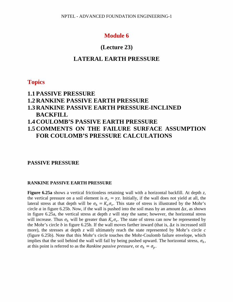
NPTEL - ADVANCED FOUNDATION ENGINEERING-1

Module 6

(Lecture 23)

LATERAL EARTH PRESSURE

Topics

1.1 PASSIVE PRESSURE 1.2 RANKINE PASSIVE EARTH PRESSURE 1.3 RANKINE PASSIVE EARTH PRESSURE-INCLINED

BACKFILL 1.4 COULOMB’S PASSIVE EARTH PRESSURE 1.5 COMMENTS ON THE FAILURE SURFACE ASSUMPTION

FOR COULOMB’S PRESSURE CALCULATIONS

PASSIVE PRESSURE

RANKINE PASSIVE EARTH PRESSURE

Figure 6.25a shows a vertical frictionless retaining wall with a horizontal backfill. At depth z, the vertical pressure on a soil element is 𝜎𝜎𝑣𝑣 = 𝛾𝛾𝛾𝛾. Initially, if the wall does not yield at all, the lateral stress at that depth will be 𝜎𝜎ℎ = 𝐾𝐾𝑜𝑜𝜎𝜎𝑣𝑣. This state of stress is illustrated by the Mohr’s circle 𝑎𝑎 in figure 6.25b. Now, if the wall is pushed into the soil mass by an amount Δ𝑥𝑥, as shown in figure 6.25a, the vertical stress at depth z will stay the same; however, the horizontal stress will increase. Thus 𝜎𝜎ℎ will be greater than 𝐾𝐾𝑜𝑜𝜎𝜎𝑣𝑣. The state of stress can now be represented by the Mohr’s circle b in figure 6.25b. If the wall moves farther inward (that is, Δ𝑥𝑥 is increased still more), the stresses at depth z will ultimately reach the state represented by Mohr’s circle c (figure 6.25b). Note that this Mohr’s circle touches the Mohr-Coulomb failure envelope, which implies that the soil behind the wall will fail by being pushed upward. The horizontal stress, 𝜎𝜎ℎ , at this point is referred to as the Rankine passive pressure, or 𝜎𝜎ℎ = 𝜎𝜎𝑝𝑝 .

NPTEL - ADVANCED FOUNDATION ENGINEERING-1

Figure 6.25 Rankine passive pressure

For Mohr’s circle c in figure 6.25b, the major principal stress is 𝜎𝜎𝑝𝑝 , and the minor principal stress is 𝜎𝜎𝑣𝑣. Substituting them into equation (84 from chapter 1) yields

𝜎𝜎𝑝𝑝 = 𝜎𝜎𝑣𝑣 tan2 �45 + 𝜙𝜙2� + 2𝑐𝑐 tan �45 + 𝜙𝜙

2� [6.55]

Now, let

𝐾𝐾𝑝𝑝 = Rankine passive earth pressure coefficient

tan2 �45 + 𝜙𝜙2� [6.56]

(See table 9). Hence, from equation (55),

𝜎𝜎𝑝𝑝 = 𝜎𝜎𝑣𝑣𝐾𝐾𝑝𝑝 + 2𝑐𝑐�𝐾𝐾𝑝𝑝 [6.57]

NPTEL - ADVANCED FOUNDATION ENGINEERING-1

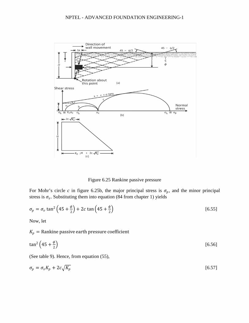
Table 9 Variation of Rankine 𝑲𝑲𝒑𝒑

Soil friction angle, 𝜙𝜙 (deg)

𝐾𝐾𝑝𝑝 = tan2(45 + 𝜙𝜙/2)

20 2.040

21 2.117

22 2.198

23 2.283

24 2.371

25 2.464

26 2.561

27 2.663

28 2.770

29 2.882

30 3.000

31 3.124

32 3.255

33 3.392

34 3.537

35 3.690

36 3.852

37 4.023

38 4.204

39 4.395

40 4.599

NPTEL - ADVANCED FOUNDATION ENGINEERING-1

41 4.815

42 5.045

43 5.289

44 5.550

45 5.828

Equation (57) produces figure 6.25c, the passive pressure diagram for the wall shown in figure 6. 25a. Note that at 𝛾𝛾 = 0,

𝜎𝜎𝑣𝑣 = 0 and 𝜎𝜎𝑝𝑝 = 2𝑐𝑐�𝐾𝐾𝑝𝑝

and at 𝛾𝛾 = 𝐻𝐻,

𝜎𝜎𝑣𝑣 = 𝛾𝛾𝐻𝐻 and 𝜎𝜎𝑝𝑝 = 𝛾𝛾𝐻𝐻𝐾𝐾𝑝𝑝 + 2𝑐𝑐�𝐾𝐾𝑝𝑝

The passive force per unit length of the wall can be determined from the area of the pressure diagram, or

𝑃𝑃𝑝𝑝 = 12𝛾𝛾𝐻𝐻

2 + 2𝑐𝑐𝐻𝐻�𝐾𝐾𝑝𝑝 [6.58]

The approximate magnitudes of the wall movements, Δ𝑥𝑥, required to develop failure under passive conditions are

Soil type Wall movement for passive condition, Δ𝑥𝑥

Dense sand 0.005H

Loose sand 0.01H

Stiff clay 0.01H

Soft clay 0.05H

Example 10

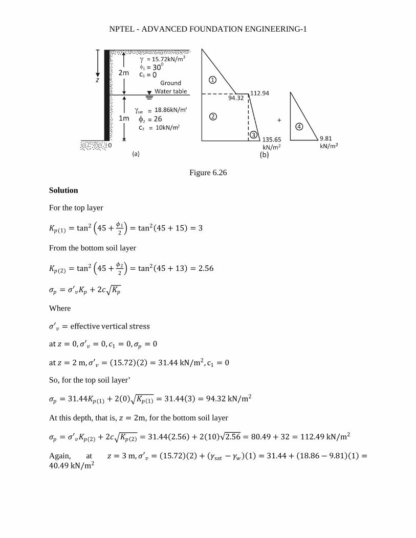
A 3-m high wall is shown in figure 6.26a. Determine the Rankine passive force per unit length of the wall.

NPTEL - ADVANCED FOUNDATION ENGINEERING-1

Figure 6.26

Solution

For the top layer

𝐾𝐾𝑝𝑝(1) = tan2 �45 + 𝜙𝜙12� = tan2(45 + 15) = 3

From the bottom soil layer

𝐾𝐾𝑝𝑝(2) = tan2 �45 + 𝜙𝜙22� = tan2(45 + 13) = 2.56

𝜎𝜎𝑝𝑝 = 𝜎𝜎′𝑣𝑣𝐾𝐾𝑝𝑝 + 2𝑐𝑐�𝐾𝐾𝑝𝑝

Where

𝜎𝜎′𝑣𝑣 = effective vertical stress

at 𝛾𝛾 = 0,𝜎𝜎′𝑣𝑣 = 0, 𝑐𝑐1 = 0,𝜎𝜎𝑝𝑝 = 0

at 𝛾𝛾 = 2 m,𝜎𝜎′𝑣𝑣 = (15.72)(2) = 31.44 kN/m2, c1 = 0

So, for the top soil layer’

𝜎𝜎𝑝𝑝 = 31.44𝐾𝐾𝑝𝑝(1) + 2(0)�𝐾𝐾𝑝𝑝(1) = 31.44(3) = 94.32 kN/m2

At this depth, that is, 𝛾𝛾 = 2m, for the bottom soil layer

𝜎𝜎𝑝𝑝 = 𝜎𝜎′𝑣𝑣𝐾𝐾𝑝𝑝(2) + 2𝑐𝑐�𝐾𝐾𝑝𝑝(2) = 31.44(2.56) + 2(10)√2.56 = 80.49 + 32 = 112.49 kN/m2

Again, at 𝛾𝛾 = 3 m,𝜎𝜎′𝑣𝑣 = (15.72)(2) + (𝛾𝛾sat − 𝛾𝛾𝑤𝑤)(1) = 31.44 + (18.86 − 9.81)(1) =40.49 kN/m2

NPTEL - ADVANCED FOUNDATION ENGINEERING-1

Hence

𝜎𝜎𝑝𝑝 = 𝜎𝜎′𝑣𝑣𝐾𝐾𝑝𝑝(2) + 2𝑐𝑐�𝐾𝐾𝑝𝑝(2) = 40.49(2.56) + (2)(10)(1.6) = 135.65 kN/m2

Note that, because a water table is present, the hydrostatic stress, u, also has to be taken into consideration. For𝛾𝛾 = 0, to 2 m,𝑢𝑢 = 0; 𝛾𝛾 = 3 m,𝑢𝑢 = (1)(𝛾𝛾𝑤𝑤) = 9.81 kN/m2.

The passive pressure diagram is plotted in figure 6.26b. The passive force per unit length of the wall can be determined from the area of the pressure diagram as follows:

Area no. Area

1 �12� (2)(94.32) = 94.32

2 (112.49)(1) = 112.49

3 �12� (1)(135.65 − 112.49) = 11.58

4 �12� (9.81)(1) = 4.905

𝑃𝑃𝑝𝑝 =≈ 223.3 kN/m

RANKINE PASSIVE EARTH PRESSURE-INCLINED BACKFILL

For a frictionless vertical retaining wall (figure 6.10) with a granular backfill (𝑐𝑐 = 0), the Rankine passive pressure at any depth can be determined in a manner similar to that done in the case of active pressure, or

𝜎𝜎𝑝𝑝 = 𝛾𝛾𝛾𝛾𝐾𝐾𝑝𝑝 [6.59]

and the passive force

𝑃𝑃𝑝𝑝 = 12𝛾𝛾𝐻𝐻

2𝐾𝐾𝑝𝑝 [6.60]

Where

𝐾𝐾𝑝𝑝 = cos𝛼𝛼 cos 𝛼𝛼+�cos 2 𝛼𝛼−cos 2 𝜙𝜙cos 𝛼𝛼−�cos 2 𝛼𝛼−cos 2 𝜙𝜙

[6.61]

As in the case of the active force, the resultant force, 𝑃𝑃𝑝𝑝 , is inclined at an angle 𝛼𝛼 with the horizontal and intersects the wall at a distance of 𝐻𝐻/3 from the bottom of the wall. The values of 𝐾𝐾𝑝𝑝 (passive earth pressure coefficient) for various values of 𝛼𝛼 and 𝜙𝜙 are given in table 10.

If the backfill of the frictionless vertical retaining wall is a 𝑐𝑐 − 𝜙𝜙 soil (figure 6.10), then

NPTEL - ADVANCED FOUNDATION ENGINEERING-1

𝜎𝜎𝑎𝑎 = 𝛾𝛾𝛾𝛾𝐾𝐾𝑝𝑝 = 𝛾𝛾𝛾𝛾𝐾𝐾′𝑝𝑝 cos𝛼𝛼 [6.62]

Where

𝐾𝐾′𝑝𝑝 = 1cos 2 𝜙𝜙

�2 cos2 𝛼𝛼 + 2 � 𝑐𝑐

𝛾𝛾𝛾𝛾� cos𝜙𝜙 sin𝜙𝜙

+�4 cos2 𝛼𝛼(cos2 𝛼𝛼 − cos2 𝜙𝜙) + 4 � 𝑐𝑐𝛾𝛾𝛾𝛾�

2cos2 𝜙𝜙 + 8 � 𝑐𝑐

𝛾𝛾𝛾𝛾� cos2 𝛼𝛼 sin𝜙𝜙 cos𝜙𝜙

� − 1 [6.63]

Table 10 Passive Earth Pressure Coefficient, 𝑲𝑲𝒑𝒑 [equation (61)

𝜙𝜙(deg) →

↓ 𝛼𝛼(deg) 28 30 32 34 36 38 40

0 2.770 3.000 3.255 3.537 3.852 4.204 4.599

5 2.715 2.943 3.196 3.476 3.788 4.136 4.527

10 2.551 2.775 3.022 3.295 3.598 3.937 4.316

15 2.284 2.502 2.740 3.003 3.293 3.615 3.977

20 1.918 2.132 2.362 2.612 2.886 3.189 3.526

25 1.434 1.664 1.984 2.135 2.394 2.676 2.987

Table 11 Values of 𝑲𝑲′𝒑𝒑

𝑐𝑐/𝛾𝛾𝛾𝛾

𝜙𝜙(deg) 𝛼𝛼(deg) 0.025 0.050 0.100 0.500

15 0 1.764 1.829 1.959 3.002

5 1.716 1.783 1.917 2.971

10 1.564 1.641 1.788 2.880

15 1.251 1.370 1.561 2.732

20 0 2.111 2.182 2.325 3.468

5 2.067 2.140 2.285 3.435

10 1.932 2.010 2.162 3.339

15 1.696 1.786 1.956 3.183

NPTEL - ADVANCED FOUNDATION ENGINEERING-1

25 0 2.542 2.621 2.778 4.034

5 2.499 2.578 2.737 3.999

10 2.368 2.450 2.614 3.895

15 2.147 2.236 2.409 3.726

30 0 3.087 3.173 3.346 4.732

5 3.042 3.129 3.303 4.674

10 2.907 2.996 3.174 4.579

15 2.684 2.777 2.961 4.394

The variation of 𝐾𝐾′𝑝𝑝 with 𝜙𝜙,𝛼𝛼, 𝑐𝑐/𝛾𝛾𝛾𝛾 is given in table 11 (Mazindrani and Ganjali, 1997).

COULOMB’S PASSIVE EARTH PRESSURE

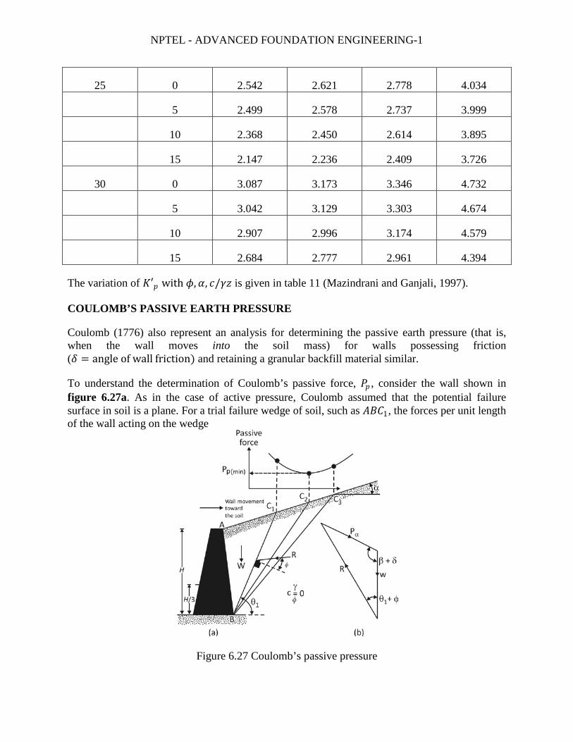
Coulomb (1776) also represent an analysis for determining the passive earth pressure (that is, when the wall moves into the soil mass) for walls possessing friction (𝛿𝛿 = angle of wall friction) and retaining a granular backfill material similar.

To understand the determination of Coulomb’s passive force, 𝑃𝑃𝑝𝑝 , consider the wall shown in figure 6.27a. As in the case of active pressure, Coulomb assumed that the potential failure surface in soil is a plane. For a trial failure wedge of soil, such as 𝐴𝐴𝐴𝐴𝐴𝐴1, the forces per unit length of the wall acting on the wedge

Figure 6.27 Coulomb’s passive pressure

NPTEL - ADVANCED FOUNDATION ENGINEERING-1

1. The weight of the wedge, W 2. The resultant, R, of the normal and shear forces on the plane 𝐴𝐴𝐴𝐴1 3. The passive force, 𝑃𝑃𝑝𝑝

Figure 6.27 shows the force triangle at equilibrium for the trial wedge 𝐴𝐴𝐴𝐴𝐴𝐴1. From this force triangle, the value of 𝑃𝑃𝑝𝑝 can be determined because the direction of all three forces and the magnitude of one force are known.

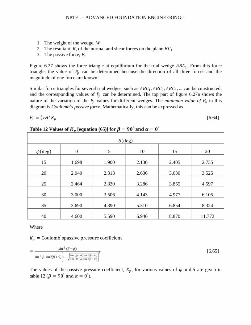
Similar force triangles for several trial wedges, such as 𝐴𝐴𝐴𝐴𝐴𝐴1,𝐴𝐴𝐴𝐴𝐴𝐴2,𝐴𝐴𝐴𝐴𝐴𝐴3, … can be constructed, and the corresponding values of 𝑃𝑃𝑝𝑝 can be determined. The top part of figure 6.27a shows the nature of the variation of the 𝑃𝑃𝑝𝑝 values for different wedges. The minimum value of 𝑃𝑃𝑝𝑝 in this diagram is Coulomb’s passive force. Mathematically, this can be expressed as

𝑃𝑃𝑝𝑝 = 12𝛾𝛾𝐻𝐻

2𝐾𝐾𝑝𝑝 [6.64]

Table 12 Values of 𝑲𝑲𝒑𝒑 [equation (65)] for 𝜷𝜷 = 𝟗𝟗𝟗𝟗° 𝐚𝐚𝐚𝐚𝐚𝐚 𝜶𝜶 = 𝟗𝟗°

𝛿𝛿(deg)

𝜙𝜙(deg) 0 5 10 15 20

15 1.698 1.900 2.130 2.405 2.735

20 2.040 2.313 2.636 3.030 3.525

25 2.464 2.830 3.286 3.855 4.597

30 3.000 3.506 4.143 4.977 6.105

35 3.690 4.390 5.310 6.854 8.324

40 4.600 5.590 6.946 8.870 11.772

Where

𝐾𝐾𝑝𝑝 = Coulomb′spassive pressure coefficient

= sin 2 (𝛽𝛽−𝜙𝜙)

sin 2 𝛽𝛽 sin(𝛽𝛽+𝛿𝛿)�1−�sin (𝜙𝜙+𝛿𝛿)sin (𝜙𝜙−𝛼𝛼)sin (𝛽𝛽+𝛿𝛿)sin (𝛽𝛽+𝛼𝛼)�

2 [6.65]

The values of the passive pressure coefficient, 𝐾𝐾𝑝𝑝 , for various values of 𝜙𝜙 and 𝛿𝛿 are given in table 12 (𝛽𝛽 = 90° and 𝛼𝛼 = 0°).

NPTEL - ADVANCED FOUNDATION ENGINEERING-1

Note that the resultant passive force, 𝑃𝑃𝑝𝑝 , will act at a distance of 𝐻𝐻/3 from the bottom of the wall and will be inclined at an angle 𝛿𝛿 to the normal drawn to the back face of the wall.

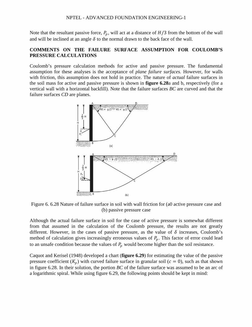
COMMENTS ON THE FAILURE SURFACE ASSUMPTION FOR COULOMB’S PRESSURE CALCULATIONS

Coulomb’s pressure calculation methods for active and passive pressure. The fundamental assumption for these analyses is the acceptance of plane failure surfaces. However, for walls with friction, this assumption does not hold in practice. The nature of actual failure surfaces in the soil mass for active and passive pressure is shown in figure 6.28a and b, respectively (for a vertical wall with a horizontal backfill). Note that the failure surfaces BC are curved and that the failure surfaces CD are planes.

Figure 6. 6.28 Nature of failure surface in soil with wall friction for (a0 active pressure case and (b) passive pressure case

Although the actual failure surface in soil for the case of active pressure is somewhat different from that assumed in the calculation of the Coulomb pressure, the results are not greatly different. However, in the cases of passive pressure, as the value of 𝛿𝛿 increases, Coulomb’s method of calculation gives increasingly erroneous values of 𝑃𝑃𝑝𝑝 . This factor of error could lead to an unsafe condition because the values of 𝑃𝑃𝑝𝑝 would become higher than the soil resistance.

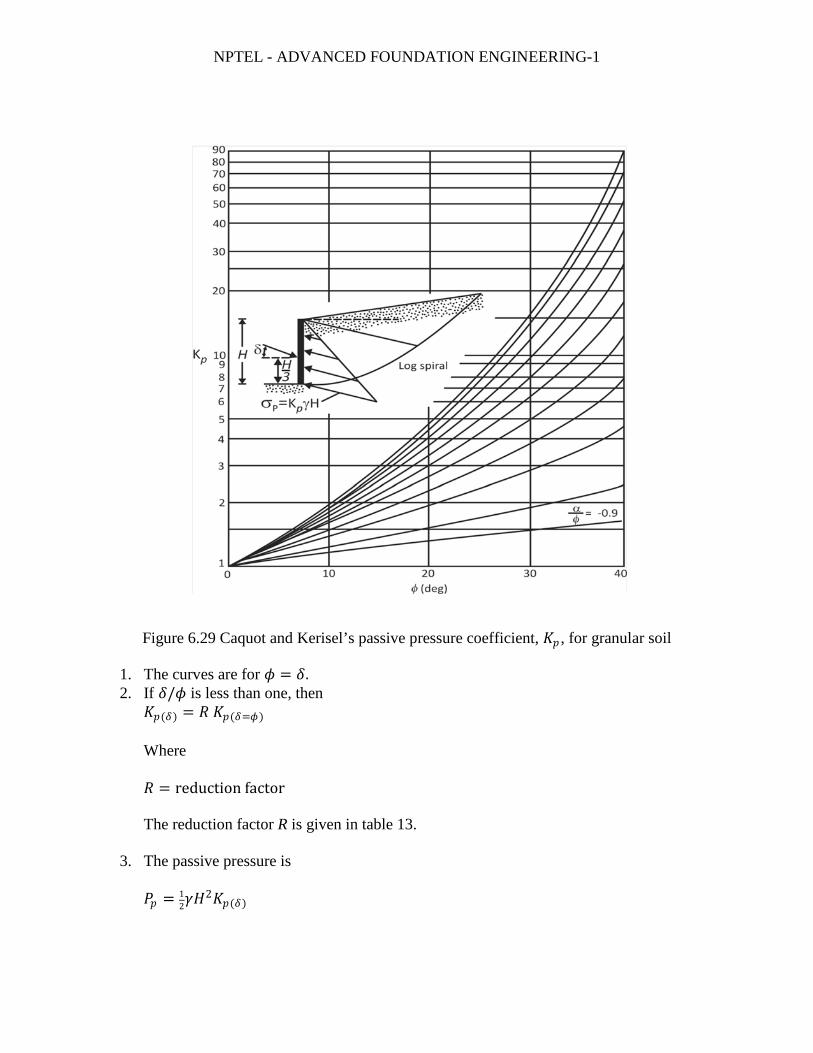
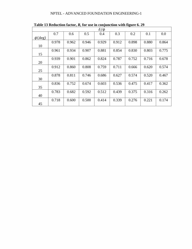
Caquot and Kerisel (1948) developed a chart (figure 6.29) for estimating the value of the passive pressure coefficient (𝐾𝐾𝑝𝑝) with curved failure surface in granular soil (𝑐𝑐 = 0), such as that shown in figure 6.28. In their solution, the portion BC of the failure surface was assumed to be an arc of a logarithmic spiral. While using figure 6.29, the following points should be kept in mind:

NPTEL - ADVANCED FOUNDATION ENGINEERING-1

Figure 6.29 Caquot and Kerisel’s passive pressure coefficient, 𝐾𝐾𝑝𝑝 , for granular soil

1. The curves are for 𝜙𝜙 = 𝛿𝛿. 2. If 𝛿𝛿/𝜙𝜙 is less than one, then

𝐾𝐾𝑝𝑝(𝛿𝛿) = 𝑅𝑅 𝐾𝐾𝑝𝑝(𝛿𝛿=𝜙𝜙) Where 𝑅𝑅 = reduction factor The reduction factor R is given in table 13.

3. The passive pressure is 𝑃𝑃𝑝𝑝 = 1

2𝛾𝛾𝐻𝐻2𝐾𝐾𝑝𝑝(𝛿𝛿)

NPTEL - ADVANCED FOUNDATION ENGINEERING-1

Table 13 Reduction factor, R, for use in conjunction with figure 6. 29 𝛿𝛿/𝜙𝜙

𝜙𝜙(deg) 0.7 0.6 0.5 0.4 0.3 0.2 0.1 0.0

10 0.978 0.962 0.946 0.929 0.912 0.898 0.880 0.864

15 0.961 0.934 0.907 0.881 0.854 0.830 0.803 0.775

20 0.939 0.901 0.862 0.824 0.787 0.752 0.716 0.678

25 0.912 0.860 0.808 0.759 0.711 0.666 0.620 0.574

30 0.878 0.811 0.746 0.686 0.627 0.574 0.520 0.467

35 0.836 0.752 0.674 0.603 0.536 0.475 0.417 0.362

40 0.783 0.682 0.592 0.512 0.439 0.375 0.316 0.262

45 0.718 0.600 0.500 0.414 0.339 0.276 0.221 0.174