NPL REPORT AS 3 Comparison of methods for the measurement of
49
National Physical Laboratory | Hampton Road | Teddington | Middlesex | United Kingdom | TW11 0LW Switchboard 020 8977 3222 | NPL Helpline 020 8943 6880 | Fax 020 8943 6458 | www.npl.co.uk NPL REPORT AS 3 Comparison of methods for the measurement of hydrocarbon dew point of natural gas Andrew Brown Martin Milton Gergely Vargha Richard Mounce Chris Cowper Andrew Stokes Andy Benton Mike Bannister Andy Ridge Dave Lander Andrew Laughton May 2007
Transcript of NPL REPORT AS 3 Comparison of methods for the measurement of

National Physical Laboratory | Hampton Road | Teddington | Middlesex | United Kingdom | TW11 0LW
Switchboard 020 8977 3222 | NPL Helpline 020 8943 6880 | Fax 020 8943 6458 | www.npl.co.uk
NPL REPORT AS 3 Comparison of methods for the measurement of hydrocarbon dew point of natural gas Andrew Brown Martin Milton Gergely Vargha Richard Mounce Chris Cowper Andrew Stokes Andy Benton Mike Bannister Andy Ridge Dave Lander Andrew Laughton May 2007


NPL Report AS 3
Comparison of methods for the measurement of hydrocarbon dew point of natural gas
May 2007
Andrew Brown, Martin Milton, Gergely Vargha, Richard Mounce1, Chris Cowper1, Andrew Stokes2, Andy Benton2, Mike Bannister2,
Andy Ridge3, Dave Lander4 and Andrew Laughton5
1 EffecTech Ltd., Dove Fields, Uttoxeter, UK. ST14 8HU 2 Michell Instruments Ltd., Nuffield Close, Cambridge, UK. CB4 1SS
3 Orbital Ltd, Cold Meece, Swynnerton, UK. ST15 0QN 4 National Grid, National Grid House, Warwick, UK. CV34 6DA 5 Advantica Ltd., Ashby Road, Loughborough, UK. LE11 3GR

NPL Report AS 3
2
© Crown Copyright 2007
Reproduced by permission of the Controller of HMSO And Queen’s Printer for Scotland
ISSN 1754-2928
National Physical Laboratory Hampton Road, Teddington, Middlesex, TW11 0LW
We gratefully acknowledge the financial support of the UK Department of Trade and Industry (Measurement for Innovators Programme and National Measurement System)
Approved on behalf of the Managing Director, NPL by Dr Stuart Windsor, Business Leader, Analytical Science Team
NPL Report AS 3
3
EXECUTIVE SUMMARY Measurement of the hydrocarbon dew point of natural gas is crucial when determining whether gas can be transported safely through national and international pipeline networks. This report summarises the results of a study undertaken to compare the performance of direct and indirect methods for determining the hydrocarbon dew point of a wide range of real and synthetic natural gases. The results obtained from six analytical methods (one automatic chilled mirror instrument, one manual chilled mirror instrument, two laboratory gas chromatographs and two process gas chromatographs) are presented and the comparative results are compared in detail. The conclusions from the work discuss the relative performance of the different methods and consider how they vary when used with real and synthetic gases of different compositions. The difficulties inherent in measuring a ‘true’ value of hydrocarbon dew point are also discussed.

NPL Report AS 3
4
CONTENTS Executive Summary 3 1 Introduction 5 1.1 Hydrocarbon dew point 5 1.2 Measurement of hydrocarbon dew point 6 2 Experimental 7 2.1 Overview 7 2.2 Preparation of Primary Reference Gas Mixtures of synthetic natural gas 7 2.3 Sampling and stability of real natural gas mixtures 7 2.4 Automatic chilled mirror instrument 9 2.5 Manual chilled mirror instrument 11 2.6 Laboratory GC 1 11 2.7 Laboratory GC 2 12 2.8 Process GC 3 12 2.9 Process GC 4 13 2.10 Measurement of water content 13 2.11 Calculations 13 2.12 Use of different equations of state 14 3. Synthetic mixtures of natural gas 15 3.1 Introduction 15 3.2 Results 17 3.3 Discussion 23 4. Real samples of natural gas 26 4.1 Introduction 26 4.2 Results 27 4.3 Discussion 35 5. Conclusions 38 6. Further information 38 References 39 Annexes Annex A - Calibration and comparison of chilled mirror thermometer and pressure sensor
40
Annex B - Calculation of water dew curves for water vapour 42 Annex C - Composition of vapour and liquid phases of synthetic mixtures of natural gas
43

NPL Report AS 3
5
1. INTRODUCTION 1.1. Hydrocarbon dew point Measurement of the hydrocarbon dew point of natural gas is crucial in determining whether gas can be transported safely through national and international pipeline networks. Maximum legislative levels for hydrocarbon dew point are set in order to prevent the formation of liquid condensate in the pipeline, which could have severe consequences for the safe transportation of natural gas. The complex nature of the condensation process in a multi-component hydrocarbon mixture leads to there being several ways of defining the ‘hydrocarbon dew point’. The definition given by ISO 14532 [1] is the:
“Temperature above which no condensation of hydrocarbons occurs at a specified pressure.” NOTE 1: At a given dew point temperature there is a pressure range within which retrograde condensation can occur. The cricondentherm defines the maximum temperature at which this condensation can occur. NOTE 2: The dew point line is the locus of points for pressure and temperature which separates the single phase gas from the biphasic gas-liquid region.
An example of a hydrocarbon dew point curve for a typical natural gas mixture is shown in Figure 1.
0
20
40
60
80
100
-30 -20 -10 0 10 20Temperature (C)
Pres
sure
(bar
)
Mixture exists in gas and
liquid phases
Mixture wholly in gas phase
Cricondentherm
Figure 1. Typical hydrocarbon dew point curve. The cricondentherm (indicated by the red arrow) is defined as the maximum temperature at which condensation can occur (at any pressure).

NPL Report AS 3
6
If defined as above, the hydrocarbon dew point of a pre-specified gas cannot be measured in practice because detection of the onset of condensation requires the observation of the first molecule of liquid condensate - this is unachievable experimentally. Discussions are therefore ongoing within an ISO (International Organization for Standardization) committee (ISO/TC193/SC1) to redefine the dew point as a ‘technical’ or ‘measurable’ dew point. This is discussed in detail in Section 4.3.4. 1.2. Measurement of hydrocarbon dew point The methods that can be used to measure the hydrocarbon dew point of natural gas may be classified as being direct methods or indirect methods. The two ‘direct’ methods studied in this work, which used a manual chilled mirror instrument (MCMI) and an automatic chilled mirror instrument (ACMI), detect the formation of a film of liquid condensate on the cooled surface of a mirror. The MCMI method relies on a skilled operator to detect manually the formation of the film, whereas the ACMI is a fully automated process (see Section 2 for full details). An advantage of these methods is that they provide a direct observation of the formation of film on the mirror, but the measurement may be dependent on the operator of the manual instrument, or the sensitivity setting of the automatic instrument. The most common ‘indirect’ method uses gas chromatography (GC) to determine the composition of the gas mixture. A thermodynamic equation of state (EoS) is then used to calculate the hydrocarbon dew curve. The measurement of the composition of the gas, which is usually automated, can be carried out to a high accuracy, but this method for determining dew point is heavily reliant on the validity of the equation of state used. Additionally, heavier (C11+) hydrocarbon components (which affect the dew temperature significantly) may be present in very low quantities that are below the limit of detection of the instrument. Indirect methods, however, benefit from being able to provide a full dew curve, enabling determination of the hydrocarbon dew point at any pressure. A further approach, not studied here, is the potential hydrocarbon liquid content (PHLC) method [2] which measures gravimetrically the amount of liquid condensate formed at a pre-defined pressure and temperature. This report compares the performance of an ACMI, MCMI, and a series of laboratory and process GCs in determining the hydrocarbon dew point of a series of synthetic and real natural gases.

NPL Report AS 3
7
2. EXPERIMENTAL 2.1. Overview The first part of the study determined the dew points of five synthetic natural gas mixtures of limited composition; the second part studied seven real natural gas mixtures sampled from gas fields around the British Isles. The experimental methods used in each part of the study are summarised in Table 1 and described in detail below.
Method Synthetic gas mixtures
Real natural gases
ACMI MCMI
Lab GC 1 Lab GC 2
Process GC 3 Process GC 4
Table 1. Summary of experimental methods used in the study.
2.2. Preparation of Primary Reference Gas Mixtures of synthetic natural gas All synthetic standards were prepared gravimetrically using ‘pure’ gases and liquids, each component being added separately using either loop injection (for all liquids and those gaseous components with a required mass of < 15g) or direct gas transfer (for gaseous components with a required mass of > 15g), as described below:
• Loop injection: Transfer of the gas or liquid directly into the sample cylinder via a minimised-dead volume valve. To calculate the mass of gas or liquid added, the loop was weighed (against a tare loop) before and after transfer.
• Direct gas transfer: addition of the gas to the sample cylinder via 1/16″ internal diameter Silcosteel-coated stainless steel tubing. The sample cylinder was weighed (against a tare cylinder) on a single-pan balance.
A full purity analysis was carried out on each ‘pure’ component and the gravimetric amount fraction of each component was calculated from the mass of each component added, its molecular mass and purity analysis. Uncertainties were calculated following ISO 6141 [3]. 2.3. Sampling and stability of real natural gas mixtures The samples were obtained using the evacuated cylinder method described in Annex F of ISO 10715 [4]. A schematic diagram of the sampling apparatus is shown in Figure 2 and a brief synopsis of the sampling method is given below:

NPL Report AS 3
8
vent
vent
sample cylinder
Sampling equipment
(connected to main gas line)
sample line
valve V2
valve V3
valve V4
valve V1
vent
vent
sample cylinder
Sampling equipment
(connected to main gas line)
sample line
valve V2
valve V3
valve V4
valve V1
Figure 2. Schematic diagram of set-up used to sample real natural gases. Synopsis of sampling method:
1. Purge V1 and the stub to the main gas line prior to connecting sampling equipment. Fully open and close five times, venting to atmosphere.
2. Connect the sampling equipment to V1. 3. Connect the evacuated sample cylinder with both V3 and V4 closed as received.
Close V2. Check that the system is leak tight by partially opening and closing V1. 4. Purge the sample line five times: Ensuing that you stand on one side of the
sampling system (not directly in line), fully open V1 to equalise the main gas line pressure into the sampling equipment. Close V1. Open V2 to release the pressure. Close V2.
5. With V2 closed, fully open V1. 6. Open V3 slowly, once only, until fully open. 7. Close V3. Close V1. 8. Open V2 to vent the sample gas to atmospheric pressure. 9. Disconnect the sample vessel from the sampling system and cap the vessel. 10. Disconnect the sampling equipment from V1.
In order to confirm that the composition of the real gas samples did not change during the course of the study (through contamination or decay), the samples were analysed using one of the GC methods (Lab GC 1) at the start and conclusion of the work. Figure 3 shows the calculated hydrocarbon dew curve for one of the samples before and after the study. For this, and all the other samples, no change in results was observed beyond any variation which can reasonably be expected from repeated analysis.

NPL Report AS 3
9
20
30
40
50
60
70
0 2 4 6 8 10Temperature (C)
Pres
sure
(bar
)
StartEnd
Figure 3. Calculated hydrocarbon dew curve of real Gas A measured at the start and end of the study. Both analyses were carried out using Lab GC 1.
2.4. Automatic chilled mirror instrument [Michell Condumax II] 2.4.1. Background to instrument development The Condumax II instrument applies a unique optical detection method developed specifically for the measurement of hydrocarbon dew point in natural gas. This involves monitoring the decrease in intensity of scattered light from a conical, abraded metal surface, which achieves a very high sensitivity to the low surface tension film characteristic of hydrocarbon condensates. This patented detection method resulted from a project at Shell Thornton Research Centre and was first presented at the 1986 International Congress of Gas Quality [5]. Michell Instruments became the onward technical development and commercial partners to utilise this technology to provide on-line hydrocarbon dew point measurement solutions to the global natural gas industries. The first Michell version, model HDM100, designed for permanent site installation was sold in 1986. Further development of the analyser package, comprising safe area control electronics and field based sensor cell within the sampling system, resulted in the original Condumax and in September 2005 the introduction of Condumax II as a flameproof certified version suitable for wholly hazardous area installation. The instrument has been designed to provide measurements of hydrocarbon dew point equivalent to those from a MCMI. Calculations have estimated that a condensate concentration of 70 mg.m-3 can be detected using a MCMI, and it is believed that the Condumax II instrument detects a similar concentration of condensate when operated at its standard sensitivity setting (see below). 2.4.2. Analysis The ACMI was operated in two modes:

NPL Report AS 3
10
• Standard (275 mV) sensitivity setting. The default sensitivity setting chosen to provide results that are broadly equivalent to those from a MCMI.
• Adaptive trigger point (ATP) mode. The sensitivity of the instrument is varied by increasing the trigger level of the instrument linearly with pressure. It is proposed that this allows for the fact that there is more gas in the cell at higher pressures, meaning that if the sensitivity level remains constant, a thicker film of condensate is needed before being detected by the instrument. This approach allows reproduction of the retrograde behaviour of a hydrocarbon dew curve and is confirmed by experimental results [6].
The sensitivity calibration chart in Figure 4 shows the relationship between the chosen sensitivity setting of the instrument and the measured hydrocarbon dew point. At the standard sensitivity setting of 275 mV, good repeatability between analyses of the same gas is observed, whereas lower sensitivity settings show a larger variability in results, and much higher measured hydrocarbon dew points.
-15
-10
-5
0
5
10
15
20
0
100
200
300
400
500
600
Sensitivity (mV)
Mir
ror
tem
pera
ture
(C)
Low 1 - Run 1Low 1 - Run 2Low 2 - Run 1Low 2 - Run 2Mid 1 - Run 1Mid 1 - Run 2Mid 2 - Run 1Mid 2 - Run 2High 1 - Run 1High 1 - Run 2
Figure 4. Mirror temperature as a function of signal response (‘sensitivity’) measured by the ACMI for the five synthetic natural gas mixtures. All data were recorded at a pressure of 27 bar (gauge). Note that the presence of elbows in the sensitivity curves is an artefact of plotting a line through a limited number of data points.
Key features of the procedure used with the ACMI were:
• Before analyses were carried out, the system was purged with the mixture under test (at a low flow rate) for 30-60 minutes.
• Measurements were carried out at a range of pressures, usually 20, 27, 35 and 45 bar (gauge). In general, a pressure of 27 bar (gauge) is used for field applications in the UK.
• 10-15 repeat analyses were carried out for each gas at each pressure. • The rate of cooling of the mirror around the film formation point can be as low as
0.05 ºC.s-1. • The operation of the temperature sensor in the instrument was validated through
measurement of a 10% n-butane in nitrogen gas standard (see Annex A).

NPL Report AS 3
11
2.5. Manual chilled mirror instrument [Chandler model A-2 Dew Point Tester] 2.5.1. Analysis Key features of the procedure used with the MCMI were:
• Assessment of the film formation was carried out every 0.5 °C. • The temperature was recorded using an alcohol in glass thermometer with a range
of –100 °C to +10 °C with 1 °C graduations. • The thermometer was calibrated by NPL to an expanded uncertainty of 0.5 °C and
tested through measurement of a 10% n-butane in nitrogen gas standard (see Annex A).
2.6. Laboratory GC 1 (‘Lab GC 1’) [Danalyser 500 + HP 4890 GC] 2.6.1. Instrument Danalyser 500 - configured as described in ISO 6974-5 [7] for measurement of N2, CO2, and C1 to C5 hydrocarbons. The instrument was calibrated using seven certified reference materials (CRMs) using the method described in ISO 6143 [8], generating a polynomial response function for each component.
HP 4890 GC - configured as described in ISO 23874 [9] for measurement of C5 to C12 hydrocarbons. This instrument, which had a flame ionisation detector (FID), was calibrated using a single CRM. Detailed experimental parameters are given below:
• 30 m non-polar methyl silicone phase (CP-Sil 5) capillary column. Internal diameter = 0.53 mm, film thickness = 2 μm.
• Column temperature program: 35 °C for 3.5 min, ramp to 200 °C at 6 °C.min-1. • Sample: 1 ml (split 1:3 column:vent). • Valve temperature: 100 °C. • FID temperature: 225 °C.
Due to GC baseline instability, a large expanded uncertainty (30-40%) should be applied to the C11 & C12 amount fractions The HP 4890 GC showed a response to concentration ratio that was proportional to carbon number for components up to C8. The C9 and C10 species showed responses that were high in proportion to the carbon number by about 8% and 15% (relative) respectively. 2.6.2. Analysis
Key features of the analytical procedure used with Lab GC 1 were:
• All components up to n-C6, benzene, toluene, cyclohexane and methylcyclohexane were measured and reported individually.
• For the analysis of the synthetic natural gas mixtures, the n-alkanes n-C7 to n-C10 were measured by direct calibration against traceable reference gas mixtures standards.

NPL Report AS 3
12
• For the analysis of the natural gas samples, all other C7+ alkanes, and unidentified C8+ aromatics and naphthenes were grouped by carbon number fraction (with the assumption that all isomers had the same response factor as the n-alkanes present in the calibration gas). Each individual unidentified component within these fractions had a boiling point calculated on the basis of retention time. From this, the average boiling point of the fraction was calculated by weighting each measured quantity by its calculated boiling point, as described in ISO 23874 [9]. The fractions were allocated a specific gravity (SG) value identical to that of the relevant n-alkane.
• Helium, hydrogen and oxygen, when found, were measured by direct calibration. • Four or five repeat analyses were carried out per mixture. • The hydrocarbon dew curves were calculated by use of the composition data from
the GC and the RKS equation of state [10]. 2.7. Laboratory GC 2 (‘Lab GC 2’) [Danalyser 500 + Varian 3400 GC] 2.7.1. Instrument Danalyser 500 unit - see Section 2.6.1 for full details. Varian 3400 GC – configured in a similar manner to the HP 4890 GC (see Section 2.6.1 for the measurement of C5 to C12 hydrocarbons. The Varian GC showed good carbon counting behaviour with a maximum uncertainty of approximately 2% relative. 2.7.2. Analysis Analysis and data processing were carried out in the same manner as for Lab GC 1 (section 2.6.2). 2.8. Process GC 3 [Danalyser 700] 2.8.1. Instrument Process GC with thermal conductivity detector (TCD) and FID, and three valves (one 6-port and two 10-port). All components were fitted into a single oven operated isothermally at 80°C. 2.8.2. Analysis Key features of the analytical procedure used with Process GC 3 were:
• All components up to n-C6, benzene, toluene, cyclohexane and methyl cyclohexane were measured and reported individually.
• C7 to C9 hydrocarbons were measured as carbon number fraction groups. • C10+ hydrocarbons were measured as one single backflushed group. The
quantification of this group was found to be relatively poor due to a sloping baseline.
• The instrument was not optimised for multi-level calibration. • Analysis time was < 10 min.

NPL Report AS 3
13
• Each fraction was assigned the same boiling point as calculated for Lab GC 1, and an SG value identical to that of the relevant n-alkane.
• The hydrocarbon dew curves were calculated by use of the composition data from the GC and the RKS equation of state.
2.9. Process GC 4 [Orbital ‘all in one’] system 2.9.1. Instrument Process GC system based on a Siemens Maxus Edition II instrument with three detectors: TCD (for measurement of all components up to n-C6), FID (for C6 to C12 hydrocarbons and flame photometric detector (FPD) (for sulphur containing species). 2.9.2. Analysis Key features of the analytical procedure used with Process GC 4 were:
• All components up to n-C6, benzene, toluene, cyclohexane and methyl cyclohexane were measured and reported individually.
• C6 to C12 hydrocarbons were measured as carbon number fraction groups. The boiling point and specific gravity of each fraction was calculated automatically.
• Hydrocarbon dew points were calculated automatically by the instrument’s software.
2.10. Measurement of water content The water content of each real gas sample was determined using a solid-state silicon-based instrument Messer FM62 PRV instrument operated at atmospheric pressure. To avoid problems associated with obtaining a representative sample, all samples were purged for a sufficient period of time prior to analysis. The water content of each sample was determined twice - before and after ‘push purge’ (re-zeroing of the instrument). It is the latter results that are used in this study. The response of the instrument to a dry zero gas and a range of gases with known water content (up to 120 μmol/mol) was determined before and after analysis of the real natural gases. Typically, a maximum of 2 μmol/mol difference was observed between these two analyses. 2.11. Calculations For the Lab GC 1, Lab GC 2 and Process GC 3 instruments, hydrocarbon dew point calculations were carried out using GasVLe add-in version 2.0 and the RKS equation of state. The dew points determined by Process GC 4 were calculated automatically by the instrument’s software. All water dewlines were calculated using the RKS equation of state modified by setting all interaction parameters Kij = 0.5. Further discussion of the calculation of water dewlines can be found in Annex B.

NPL Report AS 3
14
2.12. Use of different equations of state Figure 5 shows the hydrocarbon dew curve of one of the real gas mixture calculated by the RKS and two other commonly-used equations of state: PR (Peng Robinson) [11] and LRS (London Research Station [12] – a variant of RKS with different functional forms for some constants). All three equations of state are cubic in form.. At the cricondentherm, a difference of more than 2 °C is observed between the hydrocarbon dew points calculated by PR and other equations of state - this is due to the PR equation of state over-estimating the vapour pressure of the heavier components, hence giving a lower temperature for the onset of condensation. The 2 °C difference gives an indication of the uncertainty that the selection of an equation of state can contribute to the overall uncertainty of an indirect method of analysis.
10
20
30
40
50
60
-8 -6 -4 -2 0 2Temperature (C)
Pres
sure
(bar
)
RKSLRSPR
Figure 5. Hydrocarbon dew curve of a real natural gas mixture calculated using three equations of state: RKS, LRS & PR.

NPL Report AS 3
15
3. SYNTHETIC MIXTURES OF NATURAL GAS 3.1 Introduction The composition of the synthetic gas mixtures used in the first part of the study was designed to encompass the hydrocarbon condensation rates of gases from gas fields across the British Isles, including those of the most extreme compositions. An example of the wide variation in condensation rates of typical natural gas samples from five off-shore fields is shown in Figure 6:
0
100
200
300
400
500
0 1 2 3 4 5Temperature below dewpoint (C)
Con
dens
ate
(mg.
m-3
)
Gas 1Gas 2Gas 3Gas 4Gas 5
Figure 6. Calculated condensation rates of natural gases obtained from five different UK gas fields.
The mixtures prepared for the study were selected to represent three different rates of hydrocarbon condensation:
• ‘Mid’ condensation rate (two mixtures) – selected to be representative of the gases found in most UK gas fields.
• ‘High’ (one mixture) – selected to investigate whether, as envisaged, a high condensation rate leads to minimal differences between the dew points measured by the different analytical methods.
• ‘Low’ (two mixtures) – selected to be the most challenging mixtures. The samples contained all (straight-chain) n-isomers from C1 up to C8, C9 or C10; benzene; toluene and cyclohexane – the gravimetric composition and expanded uncertainty of each mixture is shown in Tables 2a & 2b and the calculated hydrocarbon dew curves and condensation rate of each mixture is shown in Figures 7 and 8 respectively.

NPL Report AS 3
16
Amount fraction (μmol/mol) Component
High Mid 1 Mid 2 Low 1 Low 2 methane 902309 893411 922325 986879 973065 ethane 68677 77122 63712 7059 16081
propane 17107 22104 10492 4597 8781 n-butane 8480 5428 1582 782.1 904.7 n-pentane 2653 1326 946.3 358.2 533.9 n-hexane 514.2 319.6 440.4 99.11 294.9 benzene 61.03 41.90 139.8 35.36 97.86 toluene 24.63 32.25 85.88 30.05 58.53
cyclohexane 45.23 55.79 59.19 31.60 50.10 n-heptane 93.83 119.7 157.5 59.23 72.74 n-octane 12.17 13.61 32.20 34.86 24.90 n-nonane 0.03 10.18 15.85 21.75 17.63 n-decane 0.01 0.03 0.05 9.84 11.75
Table 2a. Composition of synthetic gas mixtures. The figures in italics are those components where the ‘pure’ component was not added to the mixtures – the content is made up entirely of impurities from other components.
Expanded gravimetric uncertainty (% relative) Component
High Mid 1 Mid 2 Low 1 Low 2 methane 0.011% 0.010% 0.010% 0.001% 0.001% ethane 0.11% 0.10% 0.13% 0.06% 0.04%
propane 0.31% 0.24% 0.54% 0.06% 0.04% n-butane 0.47% 0.04% 0.12% 0.25% 0.23% n-pentane 0.08% 0.12% 0.16% 0.44% 0.32% n-hexane 0.26% 0.37% 0.31% 0.18% 0.49% benzene 0.18% 0.25% 0.09% 0.35% 0.14% toluene 0.37% 0.28% 0.12% 0.36% 0.20%
cyclohexane 0.22% 0.18% 0.18% 0.37% 0.25% n-heptane 0.15% 0.13% 0.67% 0.20% 0.18% n-octane 0.60% 0.54% 0.26% 0.26% 0.37% n-nonane - 0.64% 0.45% 0.36% 0.47% n-decane - - - 0.70% 0.62%
Table 2b. Relative expanded uncertainty of each component in the synthetic gas mixtures.

NPL Report AS 3
17
0
20
40
60
80
100
-80 -60 -40 -20 0
Temperature (C)
Pres
sure
(bar
)
Mid 1Mid 2HighLow 1Low 2
Figure 7. Calculated hydrocarbon dew curves of the synthetic natural gas mixtures.
0
100
200
300
400
500
0 1 2 3 4 5
Temperature below dewpoint (C)
Con
dens
ate
(mg.
m-3
)
Mid 1Mid 2HighLow 1Low 2
Figure 8. Calculated condensation rate of the synthetic natural gas mixtures. 3.2 Results Each of the five synthetic mixtures were analysed by two methods, ACMI (operated at the standard (275 mV) sensitivity setting) and Lab GC 1 (operated as detailed in Section 2.6). Figures 9 to 13 compare the results from these instruments with the dew curves calculated for the gravimetric compositions Table 2a, and the key findings for each gas are given beneath the charts. All data are plotted using pressures expressed as bar (absolute). The expanded (right hand) plots for each gas also show an estimate for the expanded uncertainty of the Lab GC 1 results at the cricondentherm. However these uncertainties, which are typically between ± 0.2 ºC and ± 0.4 ºC, only account for the errors arising from the analytical procedure, and do not include any contribution from the calculation method. An indication of the uncertainty arising from the selected equation of state can be obtained by comparing the dew points calculated by different equations – see Section 2.12.

NP
L R
epor
t AS
3
18
3.2.
1 R
esul
ts -
Hig
h
Hig
h
020406080100
-60
-50
-40
-30
-20
-10
0
Tem
pera
ture
(C)
Pressure (bar)
Gra
vim
etric
Lab
GC
1
ACM
I (27
5mV)
Hig
h
203040506070
-12
-11
-10
-9-8
-7-6
-5-4
Tem
pera
ture
(C)
Pressure (bar)
Fi
gure
9. R
esul
ts o
btai
ned
for t
he a
naly
sis
of s
ynth
etic
mix
ture
‘Hig
h’. T
he ri
ght-h
and
plot
is a
n ex
pans
ion
of th
e le
ft-ha
nd p
lot.
Key
find
ings
•
This
is th
e on
ly m
ixtu
re w
here
the
Lab
GC
1 d
ata
give
hig
her d
ew te
mpe
ratu
res t
han
the
grav
imet
ric d
ata.
The
am
ount
frac
tion
mea
sure
d by
Lab
GC
1 fo
r n-C
7 is
2.5
% h
ighe
r tha
n th
e gr
avim
etric
val
ue (a
lthou
gh th
e m
easu
red
amou
nt fr
actio
n of
n-C
8 is
0.1
% lo
wer
than
the
grav
imet
ric v
alue
).
• Th
e A
CM
I da
ta s
how
s un
usua
l ‘n
on-r
etro
grad
e’ b
ehav
iour
aro
und
the
cric
onde
nthe
rm.
This
was
orig
inal
ly p
ropo
sed
to b
e du
e to
in
adeq
uate
flus
hing
of h
eavi
er c
ompo
nent
s bet
wee
n re
adin
gs, o
r moi
stur
e in
terf
eren
ce, f
urth
er in
vest
igat
ion
reve
aled
the
need
the
chan
ge
the
sens
itivi
ty o
f the
inst
rum
ent w
ith in
crea
sing
sam
ple
pres
sure
. Thi
s ‘a
dapt
ive
trigg
er p
oint
’ app
roac
h w
as n
ot te
sted
on
the
synt
hetic
ga
s mix
ture
s.

NP
L R
epor
t AS
3
19
3.2.
2 R
esul
ts -
Mid
1
Mid
1
020406080100
-60
-50
-40
-30
-20
-10
0
Tem
pera
ture
(C)
Pressure (bar)
Gra
vim
etric
Lab
GC
1
ACM
I (27
5mV)
Mid
1
102030405060
-14
-13
-12
-11
-10
-9-8
-7-6
Tem
pera
ture
(C)
Pressure (bar)
Fi
gure
10.
Res
ults
obt
aine
d fo
r the
ana
lysi
s of
syn
thet
ic m
ixtu
re ‘M
id 1
’. Th
e rig
ht-h
and
plot
is a
n ex
pans
ion
of th
e le
ft-ha
nd p
lot.
Key
find
ings
•
Exce
llent
agr
eem
ent i
s obs
erve
d be
twee
n th
e La
b G
C 1
and
gra
vim
etric
dat
a.
• Th
e A
CM
I dat
a sh
ows n
on-r
etro
grad
e be
havi
our a
roun
d th
e cr
icon
dent
herm
- se
e co
mm
ents
for m
ixtu
re H
igh.

NP
L R
epor
t AS
3
20
3.2.
3 R
esul
ts -
Mid
2
Mid
2
020406080100
-60
-50
-40
-30
-20
-10
0
Tem
pera
ture
(C)
Pressure (bar)
Gra
vimet
ric
Lab
GC
1
ACM
I (27
5mV)
Mid
2
102030405060
-12
-11
-10
-9-8
-7-6
-5-4
Tem
pera
ture
(C)
Pressure (bar)
Fi
gure
11.
Res
ults
obt
aine
d fo
r the
ana
lysi
s of
syn
thet
ic m
ixtu
re ‘M
id 2
’. Th
e rig
ht-h
and
plot
is a
n ex
pans
ion
of th
e le
ft-ha
nd p
lot.
Key
find
ings
•
This
mix
ture
has
the
lar
gest
diff
eren
ce b
etw
een
the
dew
poi
nt m
easu
red
by t
he A
CM
I (2
75 m
V)
and
the
calc
ulat
ed d
ew p
oint
at
70 m
g.m
-3 o
f con
dens
ate.
•
The
AC
MI a
naly
sis o
f thi
s mix
ture
reve
aled
a v
ery
shar
p tra
nsiti
on fr
om th
e ga
s pha
se to
liqu
id fi
lm fo
rmat
ion.

NP
L R
epor
t AS
3
21
3.2.
4 R
esul
ts -
Low
1
Low
1
020406080100
-60
-50
-40
-30
-20
-10
0
Tem
pera
ture
(C)
Pressure (bar)
Gra
vim
etric
Lab
GC
1
ACM
I (27
5mV)
Low
1
01020304050
-10
-9-8
-7-6
-5-4
-3-2
Tem
pera
ture
(C)
Pressure (bar)
Fi
gure
12.
Res
ults
obt
aine
d fo
r the
ana
lysi
s of
syn
thet
ic m
ixtu
re ‘L
ow 1
’. Th
e rig
ht-h
and
plot
is a
n ex
pans
ion
of th
e le
ft-ha
nd p
lot.
Key
find
ings
•
Mix
ture
s Low
1 &
Low
2 a
re th
e m
ost d
iffic
ult t
o sa
mpl
e du
e to
the
rela
tivel
y hi
gh c
once
ntra
tions
of C
9 & C
10.
• Th
is m
ixtu
re s
how
s th
e la
rges
t dev
iatio
n be
twee
n th
e La
b G
C 1
and
gra
vim
etric
dat
a. T
he a
mou
nt fr
actio
ns m
easu
red
by L
ab G
C 1
for
C9 an
d C
10 a
re 6
.8%
and
8.7
% lo
wer
than
the
grav
imet
ric v
alue
s. •
The
shap
e of
the
AC
MI
curv
e is
sig
nific
antly
diff
eren
t tha
n th
ose
of th
e ca
lcul
ated
cur
ves.
This
aga
in p
oint
s to
275
mV
not
bei
ng th
e op
timum
sens
itivi
ty se
tting
at h
ighe
r pre
ssur
es.

NP
L R
epor
t AS
3
22
3.2.
5 R
esul
ts -
Low
2
Low
2
020406080100
-60
-50
-40
-30
-20
-10
0
Tem
pera
ture
(C)
Pressure (bar)
Gra
vimet
ric
Lab
GC
1
ACM
I (27
5mV)
Low
2
01020304050
-8-7
-6-5
-4-3
-2-1
0
Tem
pera
ture
(C)
Pressure (bar)
Figu
re 1
3. R
esul
ts o
btai
ned
for t
he a
naly
sis
of s
ynth
etic
mix
ture
‘Low
2’.
The
right
-han
d pl
ot is
an
expa
nsio
n of
the
left-
hand
plo
t.
Key
find
ings
•
This
mix
ture
has
the
high
est d
ew p
oint
of t
he fi
ve sy
nthe
tic g
ases
. •
Larg
e va
riatio
ns w
ere
obse
rved
in
the
repe
ated
ana
lysi
s m
ade
usin
g th
e A
CM
I. Th
is m
ay h
ave
been
a c
onse
quen
ce o
f th
e lo
w g
as
pres
sure
rem
aini
ng in
the
cylin
der a
t the
tim
e of
ana
lysi
s. •
The
shap
e of
the
AC
MI c
urve
is a
gain
diff
eren
t tha
n th
ose
of th
e ca
lcul
ated
dew
poi
nt c
urve
s.

NPL Report AS 3
23
3.2.6 Results - summary Since it is common industry practice to measure hydrocarbon dew point at a pressure of 27 bar (gauge), the ACMI is optimised to measure the dew point at this pressure. The results obtained at this pressure are given in Table 3 (gauge):
Hydrocarbon dew point / °C Mixture Gravimetric Lab GC 1 ACMI
High Mid 1 Mid 2 Low 1 Low 2
-8.3 -8.7 -5.0 -3.9 -1.6
-7.9 -8.5 -4.6 -4.4 -1.5
-8.8 -10.0 -7.0 -6.7 -4.0
Table 3. Summary of results of analysis of synthetic gas mixtures. All analyses were carried out at a pressure of 27 bar.
3.3 Discussion The above results show that the hydrocarbon dew points measured by Lab GC 1 agree well with those calculated from the gravimetric composition data – the average difference at the cricondentherm is only 0.3 °C Good agreement is also observed between the results from the ACMI and the gravimetric data. The average difference at the cricondentherm is 1.9 °C, a value within the uncertainty of the measurement. (As shown in Section 2.12, the use of a different equation of state can lead to a change in calculated dew point of more than 2 °C.) Even closer agreement is obtained when the ACMI results are compared to the theoretical temperature at which 70 mg.m-3 of condensate is formed (see Figure 14). This level of condensate corresponds approximately to the ACMI sensitivity setting of 275 mV used here (and would be equivalent to 10 μmol/mol of n-decane, 11 μmol/mol of n-nonane or 14 μmol/mol of n-octane). When these data are compared, the average difference at the cricondentherm is only 0.7 °C. In conclusion, the data presented here from synthetic natural gas mixtures show that the two analytical methods used – an ACMI instrument and a laboratory GC - both reproduce the theoretical hydrocarbon dew curve well. The differences between the data sets are within the uncertainty of the experiment, which is greater than 2 °C.

NPL Report AS 3
24
15
25
35
45
55
-14 -12 -10 -8 -6 -4 -2 0 2
Temperature (C)
Pres
sure
(bar
)
Mid 1 - ACMIMid 2 - ACMIHigh - ACMILow 1 - ACMILow 2 - ACMIMid 1 - 70 mg.m3Mid 2 - 70 mg.m3High - 70 mg.m3Low 1 - 70 mg.m3Low 2 - 70 mg.m3
Figure 14. Comparison of ACMI results (lines) with the calculated cricondentherm temperature for the formation of 70 mg.m-3 of condensate (large circles) for all five synthetic gas mixtures.
To attempt to determine any trend between the data and the physical properties of the five mixtures, Table 4 shows the order of condensation rate and hydrocarbon dew point for each of the gases and compares this with the data in Figure 14.
Gas Condensation rate
Hydrocarbon dew point
ACMI v theoretical 70 mg.m-3 of condensate (Figure 14)
High Highest Low Close Mid 1 Mid Lowest Close Mid 2 Mid Mid ACMI ~ 1 °C low Low 2 Low Highest ACMI~ 1 °C high Low 1 Lowest Mid ACMI ~ 1 °C high
Table 4. Summary of results showing, for the five synthetic gas mixtures: (a) order of condensation rate, (b) order of hydrocarbon dew point, (c) closeness of agreement between the ACMI data and the theoretical dew point calculated for 70 mg.m-3 of condensate.
The two mixtures where the closest agreement is obtained between the ACMI data and the calculated dew point for 70 mg.m-3 of condensate are those with the two highest condensation rates. This supports the expectation that the dew points of fast-condensing gases are more straightforward to determine by direct observation methods. Mid 2 is the only mixture where hydrocarbon dew point measured by the ACMI is noticeably lower than the calculated dew point for 70 mg.m-3 of condensate. This mixture has the longest ‘hydrocarbon tail’ and its unusual behaviour was proposed to possibly be a subtle consequence of the composition of the condensate, or sampling issues caused by the presence

NPL Report AS 3
25
of C11 to C12 species (with measured amount fractions of 50 nmol/mol and 30 nmol/mol respectively). In order to investigate this possibility, the theoretical composition of the condensate (and vapour phase) for each of the synthetic gas mixtures was calculated at the cricondentherm pressure. The results are is shown in Annex C by means of the following plots:
• Liquid phase amount fraction (plotted as a log scale); • Liquid phase amount fraction (plotted as a fraction of the gravimetric amount fraction
of that component in the gas mixture); • Vapour phase amount fraction (plotted as a log scale); • Vapour phase amount fraction (plotted as a fraction of the gravimetric amount
fraction of that component in the gas mixture). Some differences are observed between the gas mixtures, but the order of the amount fractions of most components in the condensate generally remains constant at all temperatures below the dew point - only the amount fractions of the heaviest components (C8+) decrease significantly at lower temperatures. It can therefore be concluded that composition of the condensate is unlikely to account for the small differences between measured and theoretical hydrocarbon dew point. Indeed, these differences are well within the best available estimate of the uncertainty of the data. The data also show that, even at temperatures only a fraction of a degree below the cricondentherm, all components are present in the condensate. In fact, for mixtures High, Mid 1 and Mid 2, the most abundant species is methane. This is not intuitive and is a consequence of the fact that fact that, methane is at least an order of magnitude more abundant than any other species in the original gas mixtures. For mixtures Low 1 and Low 2 (which have the highest higher hydrocarbon content), the most abundant components in the liquid phase just below the cricondentherm are, in order, n-decane, n-nonane and methane.

NPL Report AS 3
26
4. REAL SAMPLES OF NATURAL GAS 4.1 Introduction The second part of the work reported here studied a range of seven real natural gas mixtures taken from gas fields around the British Isles. Due to the highly complex nature of real gas mixtures, these samples provided a sterner challenge to the analytical methods than the synthetic mixtures discussed in Section 3. The gases were selected to represent the extremes of composition that could be encountered in gases entering the UK network and are therefore not generally representative of those for which on-line are measurements carried out across the network. The composition of each sample (determined by Lab GC 1), along with the calculated cricondentherm pressure and temperature are shown in Table 5.
Amount fraction (μmol/mol) Component
Gas A Gas B Gas C Gas D Gas E Gas F Gas G Helium 319 470 420 329 30 80 120
Hydrogen 78 7.0 8.0 100 62 11 4.0 Oxygen + argon 269 40 60 160 30 50 40
Nitrogen 61120 41880 24600 71560 4450 8111 2600 Carbon dioxide 569 10020 4775 4713 17290 21730 6730
Methane 835100 892900 933100 859500 883200 880600 986900 Ethane 57600 39110 28140 43580 73150 62940 3360
Propane 23990 9790 5024 10650 17830 20370 130 i-butane 4863 1597 874 2253 1625 1801 30 n-butane 8909 2048 1113 3273 1968 3120 27
neo-pentane 94 49 31 101 0 0 0 i-pentane 2816 565 356 1240 216 420 7.5 n-pentane 2314 528 331 1040 143 430 7.4
2,2-dimethylbutane 85 42 39 105 1.5 5.8 1.8 2,3-dimethylbutane 121 34 29 66 5.5 23 3.4
2-methylpentane 546 124 100 307 11 57 2.1 3-methylpentane 309 63 57 173 5.3 27 1.4
n-hexane 327 161 144 399 10 69 3.8 Benzene 2.5 250 226 3.9 3.4 28 0.17
Cyclohexane 171 72 75 77 1.9 23 3.1 Toluene 0.31 32 53 0.8 0.51 6.9 0.12
Methylcyclohexane 56 56 77 46 0.61 10 2.9 Other C7 species 339 148 200 304 4.9 49 5.3
C8 fraction 22 35 88 40 0.17 4.9 1.9 C9 fraction 2.6 12 42 5.9 0.03 1.4 0.70 C10 fraction 0.03 1.2 4.8 0.35 0 0.09 0.33 C11 fraction 0 0.08 0.31 0.02 0 0 0.14 C12 fraction 0 0 0.002 0 0 0 0
Cricondentherm Gas A Gas B Gas C Gas D Gas E Gas F Gas G p / bar 48 33 31 38 45 37 15 T / °C 7.4 -8.4 -1.0 -3.7 -37.6 -23.6 -26.4
Table 5. Measured composition and cricondentherm point of the seven real natural samples used in the study (data obtained from Lab GC 1).

NPL Report AS 3
27
The condensation rate of each of the samples (calculated using the data in Table 5) is shown in Figure 15:
0
100
200
300
400
500
0 1 2 3 4 5
Temperature below dewpoint (°C)
Con
dens
ate
(mg.
m-3
)
Gas AGas BGas CGas DGas EGas FGas G
Figure 15. Calculated condensation rate of each of the real natural gas samples. 4.2 Results As summarised in Table 1, the real natural gas samples were analysed by the full suite of methods available: MCMI, ACMI, laboratory GC (two instruments) and process GC (two instruments). The instruments were operated and the data processed as described in Sections 2.4 to 2.9. Figures 16 to 22 summarise the results obtained, and the key findings for each gas are given beneath the charts. All data are plotted using pressures expressed as bar (absolute). The data plotted for the ACMI are as follows:
• For Gas B, Gas C and Gas F, two sets of ACMI data are given, relating to operation of the instrument at the standard (275 mV) sensitivity setting and in adaptive trigger point mode (see Section 2.4).
• For Gas A and Gas D, only one set of ACMI data are given, relating to operation of the instrument at the standard (275 mV) sensitivity. These samples had insufficient pressure to investigate the retrograde behaviour of the dew curve by use of the adaptive trigger point mode.
• For Gas E and Gas G, no ACMI data is given as the hydrocarbon dew point of these mixtures are below the range of the instrument.

NP
L R
epor
t AS
3
28
4.2.
1. R
esul
ts –
Gas
A
Gas
A
020406080100 -5
0-4
0-3
0-2
0-1
00
1020
Tem
pera
ture
(C)
Pressure (bar)
Lab
GC
1La
b G
C 2
Pro
cess
GC
3P
roce
ss G
C 4
ACM
I (27
5mV)
MC
MI
Wat
er d
ewlin
e
Gas
A
203040506070
02
46
810
Tem
pera
ture
(C)
Pressure (bar)
Fi
gure
16.
Res
ults
obt
aine
d fo
r Gas
A. T
he ri
ght-h
and
plot
is a
n ex
pans
ion
of th
e le
ft-ha
nd p
lot.
Key
find
ings
•
Ver
y go
od a
gree
men
t is o
bser
ved
betw
een
thre
e of
the
GC
met
hods
. Pro
cess
GC
4 re
ports
low
er d
ew p
oint
s.
• Th
is m
ixtu
re h
as th
e hi
ghes
t dew
poi
nt, s
econ
d hi
ghes
t con
dens
atio
n ra
te a
nd o
ne o
f the
low
est h
igh
hydr
ocar
bon
(C10
to C
12) c
onte
nts o
f th
e re
al sa
mpl
es. I
t is t
here
fore
rela
tivel
y st
raig
htfo
rwar
d to
ana
lyse
. •
This
gas
show
s the
seco
nd c
lose
st a
gree
men
t bet
wee
n th
e M
CM
I and
Lab
GC
resu
lts (b
ehin
d G
as D
).

NP
L R
epor
t AS
3
29
4.2.
2. R
esul
ts –
Gas
B
Gas
B
020406080100 -6
0-5
0-4
0-3
0-2
0-1
00
10
Tem
pera
ture
(C)
Pressure (bar)
Lab
GC
1La
b G
C 2
Pro
cess
GC
3P
roce
ss G
C 4
ACM
I (27
5mV)
ACM
I (AT
P)
MC
MI
Wat
er d
ewlin
e
Gas
B
102030405060
-15
-13
-11
-9-7
-5
Tem
pera
ture
(C)
Pressure (bar)
Fi
gure
17.
Res
ults
obt
aine
d fo
r Gas
B. T
he ri
ght-h
and
plot
is a
n ex
pans
ion
of th
e le
ft-ha
nd p
lot.
Key
find
ings
. •
Non
-ret
rogr
ade
beha
viou
r is o
bser
ved
for t
he A
CM
I ope
ratin
g at
a 2
75 m
V se
nsiti
vity
setti
ng. U
se o
f the
‘ada
ptiv
e tri
gger
poi
nt’ m
ode
track
s the
shap
es o
f the
cur
ve m
ore
clos
ely.
•
A re
lativ
ely
larg
e di
ffer
ence
(app
rox
6 ºC
) is f
ound
bet
wee
n th
e M
CM
I and
AC
MI d
ata
– se
e co
mm
ents
for G
as C
.

NP
L R
epor
t AS
3
30
4.2
.3. R
esul
ts –
Gas
C
Gas
C
020406080100
-60
-50
-40
-30
-20
-10
010
Tem
pera
ture
(C)
Pressure (bar)
Lab
GC
1La
b G
C 2
Pro
cess
GC
3P
roce
ss G
C 4
ACM
I (27
5mV)
ACM
I (AT
P)M
CM
IW
ater
dew
line
Gas
C
102030405060
-7-5
-3-1
13
Tem
pera
ture
(C)
Pressure (bar)
Fi
gure
18.
Res
ults
obt
aine
d fo
r Gas
C. T
he ri
ght-h
and
plot
is a
n ex
pans
ion
of th
e le
ft-ha
nd p
lot.
Key
find
ings
•
Not
e th
at th
e cr
icon
dent
herm
pre
ssur
e of
this
sam
ple
is c
lose
to 2
7 ba
r (ga
uge)
. •
This
gas
show
s a re
lativ
ely
larg
e di
ffer
ence
bet
wee
n th
e M
CM
I and
AC
MI,
and
betw
een
the
Lab
GC
s and
the
AC
MI.
•
Gas
es C
& F
show
the
clos
est a
gree
men
t bet
wee
n Pr
oces
s GC
4 a
nd L
ab G
Cs.
This
gas
has
a d
ew p
oint
in th
e te
mpe
ratu
re re
gion
whe
re
dete
rmin
atio
n by
pro
cess
GC
is k
now
n to
be
the
mos
t acc
urat
e.
• U
se o
f the
AC
MI i
n th
e ad
aptiv
e tri
gger
mod
e re
prod
uces
the
retro
grad
e sh
ape
of th
e de
w c
urve
.

NP
L R
epor
t AS
3
31
4.2.
4. R
esul
ts –
Gas
D
Gas
D
020406080100
-50
-40
-30
-20
-10
010
20
Tem
pera
ture
(C)
Pressure (bar)
Lab
GC
1La
b G
C 2
Pro
cess
GC
3P
roce
ss G
C 4
ACM
I (27
5mV)
MC
MI
Wat
er d
ewlin
e
Gas
D
152535455565
-10
-8-6
-4-2
0
Tem
pera
ture
(C)
Pressure (bar)
Fi
gure
19.
Res
ults
obt
aine
d fo
r Gas
D. T
he ri
ght-h
and
plot
is a
n ex
pans
ion
of th
e le
ft-ha
nd p
lot.
Key
find
ings
•
The
MC
MI a
nd tw
o pr
oces
s GC
s sho
w e
xtre
mel
y go
od a
gree
men
t. •
The
AC
MI (
275
mV
) and
two
Lab
GC
s sho
w g
ood
agre
emen
t. •
This
gas
show
s the
clo
sest
agr
eem
ent b
etw
een
the
MC
MI a
nd L
ab G
Cs.

NP
L R
epor
t AS
3
32
4.2.
5. R
esul
ts –
Gas
E
Gas
E
020406080100
-80
-70
-60
-50
-40
-30
-20
-10
Tem
pera
ture
(C)
Pressure (bar)
Lab
GC
1La
b G
C 2
Pro
cess
GC
3P
roce
ss G
C 4
MC
MI
Wat
er d
ewlin
e
Gas
E
152535455565
-44
-42
-40
-38
-36
-34
Tem
pera
ture
(C)
Pressure (bar)
Fi
gure
20.
Res
ults
obt
aine
d fo
r Gas
E. T
he ri
ght-h
and
plot
is a
n ex
pans
ion
of th
e le
ft-ha
nd p
lot.
Key
find
ings
•
Des
pite
the
unus
ually
low
hyd
roca
rbon
dew
poi
nt o
f th
is g
as, t
he f
our
GC
met
hods
stil
l rep
ort r
esul
ts th
at a
gree
with
in 2
°C
. The
dew
po
int i
s bel
ow th
e lo
wer
tem
pera
ture
rang
e of
the
AC
MI.
• N
atur
al g
ases
with
dew
poi
nts a
s low
as t
his s
ampl
e ar
e of
littl
e co
ncer
n to
gas
tran
spor
ters
and
regu
lato
rs.

NP
L R
epor
t AS
3
33
4.2.
6. R
esul
ts –
Gas
F
Gas
F
020406080100
-60
-50
-40
-30
-20
-10
010
Tem
pera
ture
(C)
Pressure (bar)
Lab
GC
1La
b G
C 2
Pro
cess
GC
3P
roce
ss G
C 4
ACM
I (27
5mV)
ACM
I (AT
P)
MC
MI
Wat
er d
ewlin
e
Gas
F
152535455565
-30
-28
-26
-24
-22
-20
Tem
pera
ture
(C)
Pressure (bar)
Fi
gure
21.
Res
ults
obt
aine
d fo
r Gas
F. T
he ri
ght-h
and
plot
is a
n ex
pans
ion
of th
e le
ft-ha
nd p
lot.
Key
find
ings
•
Goo
d ag
reem
ent i
s ob
serv
ed b
etw
een
all f
our
GC
met
hods
– th
e sa
mpl
e ha
s a
low
hea
vy h
ydro
carb
on c
onte
nt (
but l
arge
r th
an th
at o
f G
as E
). •
Gas
es C
& F
show
the
clos
est a
gree
men
t bet
wee
n th
e re
sults
for L
ab G
C 1
and
Pro
cess
GC
4.
• U
se o
f the
AC
MI i
n th
e ad
aptiv
e tri
gger
mod
e re
prod
uces
the
retro
grad
e sh
ape
of th
e de
w c
urve
.

NP
L R
epor
t AS
3
34
4.2
.7. R
esul
ts –
Gas
G
Gas
G
020406080100
-80
-70
-60
-50
-40
-30
-20
-10
Tem
pera
ture
(C)
Pressure (bar)
Lab
GC
1La
b G
C 2
Pro
cess
GC
3P
roce
ss G
C 4
MC
MI
Wat
er d
ewlin
e
Fi
gure
22.
Res
ults
obt
aine
d fo
r Gas
G. T
he ri
ght-h
and
plot
is a
n ex
pans
ion
of th
e le
ft-ha
nd p
lot.
Key
find
ings
•
This
gas
has
a h
ighl
y un
usua
l com
posi
tion
(due
to it
s lo
ng, b
ut v
ery
flat h
ydro
carb
on ta
il bu
t a re
lativ
ely
low
C2 t
o C
5 con
tent
) and
the
low
est c
onde
nsat
ion
rate
. •
The
data
con
firm
that
a lo
ng h
ydro
carb
on ta
il re
sults
in a
larg
e sp
read
of a
naly
tical
resu
lts.
• Th
e de
w p
oint
of t
his g
as is
bel
ow th
e lo
wer
tem
pera
ture
rang
e of
the
AC
MI.

NPL Report AS 3
35
4.3. Discussion 4.3.1. Comparison of GC methods (lab GCs v process GCs) The hydrocarbon dew points calculated by the four different GC methods at a pressure at or near to the cricondentherm are shown in Table 6:
Measured hydrocarbon dew point (°C) Gas Pressure (bar) Lab GC 1 Lab GC 2 Process GC 3 Process GC 4
A 50 7.4 6.8 6.8 5.4 B 35 -8.4 -9.7 -10.0 -7.5 C 30 -1.1 -1.6 -3.1 -1.7 D 40 -3.7 -4.8 -5.7 -6.2 E 45 -37.6 -37.5 -37.8 -36.1 F 35 -23.7 -24.5 -24.7 -23.5 G 15 -26.4 -40.1 -63.5 -51.2
Table 6. The hydrocarbon dew point of each gas determined by the four GC instruments. For each gas, the pressure of the cricondentherm (to the nearest 5 bar) has been selected for comparison.
For the first three GCs, all the measured dew points are in the order Lab GC 1 > Lab GC 2 > Process GC 3. This order illustrates the relative sensitivity of each instrument to detect the higher hydrocarbon species – even small amounts of these species can have a large effect on the calculated hydrocarbon dew point. The dew points from these three instruments have all been calculated using the RKS equation of state using similar fraction boiling points and specific gravities. The results for Process GC 4 do not follow a similar trend. This GC determined the hydrocarbon dew point (and the boiling point and specific gravity of each hydrocarbon fraction) automatically using its internal software. It is thought that the differences between the Process GC 4 results and those from the other instruments result from these differences in data processing. Despite this difference, the Process GC 4 results generally agree with those from Process GC 3. Excluding Gas G (which has a highly unusual composition), the maximum difference in measured dew point at the cricondentherm is 2.5 °C. As discussed for the synthetic gas mixtures, these methods can be said to agree within a reasonable estimate of their uncertainties. 4.3.2. Comparison of dew point instruments (MCMI v ACMI) Table 7 gives a comparison between the hydrocarbon dew points measured by the automatic and manual chilled mirror instruments. As the MCMI was only operated at a single pressure, the MCMI readings at this pressure have been compared to an ACMI result calculated by interpolation between the nearest two data points (using 275 mV sensitivity).

NPL Report AS 3
36
Measured hydrocarbon dew point (°C) Gas Pressure
(bar) ACMI (275 mV) MCMI A 50 8.2 5.0 B 34 -6.5 -12.5 C 32 2.3 -4.0 D 39 -1.8 -6.0 E 46 N/A -41.0 F 38 -19.8 -27.5 G 13 N/A -31.5
Table 7. The hydrocarbon dew point of each gas determined by the two chilled mirror instruments. For each gas, the pressure at which the measurement took place is given in brackets (all ACMI results are an interpolation between the nearest two readings). Gas E and Gas G were out of the range of the ACMI.
For all gases, the dew point measured by the ACMI is greater than that measured by the MCMI, the difference being between 3.2 °C and 7.7 °C. These differences are larger than might be expected to occur between the two methods because they both depend on direct observation of the formation of a hydrocarbon film. For Gas B and Gas F, slightly closer agreement is obtained when the ACMI is used in the adaptive trigger point mode, although the differences from the MCMI data are still 5.6 °C and 6.2 °C respectively. However, the results from the comparison of temperature measurements using an n-butane in nitrogen standards (Annex A) showed that the results from the MCMI were typically 2 °C lower than those from the automatic instrument. When taking this into account, the difference between the two chilled mirror instruments reduces to between 1.2 °C and 5.7 °C. The differences at the upper end of this range are unexpectedly large and merit further investigation. 4.3.3. Comparison of ‘process’ instruments (process GCs v ACMI) Comparison of the results between the ACMI and the GCs shows a difference in behaviour for real and synthetic gas mixtures. For all seven real samples, the dew points measured by the ACMI are greater than those from the process GCs (and indeed from all the GCs). This difference would in fact be more pronounced if the GC data were used to calculate the theoretical dew point for the formation of 70 mg.m-3 of condensate (see Section 3.3 for this discussion for the synthetic mixtures). This difference requires further investigation. One possible explanation is that it may be due to the complex nature of the real mixtures, the compositions of which are difficult to determine accurately by GC. In particular, the higher hydrocarbon species may be under-measured, not detected or misidentified. Also, unexpected components (such as very heavy oils or glycols) are likely to be not measured at all – any such species will have a disproportionately large effect on the calculated hydrocarbon dew point. Another possible cause of the difference may be factors related to the operation of the ACMI, such as the trigger point, cooling rate and cell construction.

NPL Report AS 3
37
In contrast, the dew points measured by the MCMI (which are lower that those determined by GC) show the opposite trend. The differences between the results from the two chilled mirror instrument are discussed in the section above. For the synthetic gas mixtures, the opposite effect is observed for all gases, i.e. the GC dew points are higher than those reported by the ACMI. For these mixtures (which were not analysed by either of the process GCs), the Lab GC can be said to measure the ‘correct’ dew point, as the values agree very well with those determined from the known gravimetric composition. The slightly lower dew points recorded by the ACMI can be explained by the dynamic nature of the method which requires real condensate to be formed. The GC method calculated the ‘theoretical’ dew point (the point of formation of the first molecule of condensate) – a measurement which any direct observation method cannot carry out. 4.3.4. ‘True’ value of hydrocarbon dew point In summary, the analysis of the real natural gases revealed a spread of results from the different analytical methods used – the dew points measured by the four GC methods agree within a reasonable estimate of their uncertainties, but more variability is exhibited with the chilled mirror instruments. The differences between results from method to method, and from gas to gas mean that no single method can be said to definitively measure the ‘true’ hydrocarbon dew point. For example, the GC methods may not measure trace quantities of higher hydrocarbons, or ‘unexpected’ components, whereas the chilled mirror instruments are dependent upon the detection of a liquid film, and other operational and instrumental factors. Even for the synthetic mixtures, where the dew points measured by Lab GC 1 were shown to be in very good agreement with those calculated from the gravimetric composition data, some uncertainty exists regarding the validity of the equation of state used to perform the calculations. As referred to in Section 1.1, the issue that the current definition of hydrocarbon dew point cannot be measured in practice is under discussion within ISO/TC193/SC1. The recommendation being put forward is that dew point should be redefined as a ‘technical’ or ‘measurable’ dew point to aid convergence of the determined value from the different methods of measurement. One approach would be to ensure that, when used in gas quality specifications, the term hydrocarbon dewpoint is appended by:
• the determined value, e.g. a maximum of –2 °C at pressures from 1 to 70 bar (gauge); • a maximum permissible error, e.g. ± 1.5 °C (from the accepted or true value); and • the method of determination (in case of a disputed value should be stated).
It is therefore recommended that, until such time when an industry-standard method for measuring hydrocarbon dew point is adopted, reported dew points should also contain information about the analytical method used, and any assumptions made during the analysis.

NPL Report AS 3
38
5. CONCLUSIONS The work presented in this report details the results of a comprehensive study of the measurement of the hydrocarbon dew point of real and synthetic natural gases. Six analytical methods were examined: one ACMI, one MCMI, two lab GCs and two process GCs. Analysis of synthetic natural gas mixtures showed a good agreement between the dew points measured the methods used, one lab GC and the ACMI. Although measurement of the real natural gases proved to be much more challenging, agreement was in most cases obtained between the dew points measured by the different analytical methods. The results from the four GC instruments differ by no more than 2.5 °C at the cricondentherm and can be said to agree within a reasonable estimate of their uncertainties. The chilled mirror methods show larger variability. An interesting difference in behaviour is observed when comparing the ACMI and GC results for the synthetic and real mixtures – it is proposed that this may be due to the complex nature of the real mixtures, or other effects, and merits further investigation. The results from the analysis of the real gases also show that a ‘true’ value of hydrocarbon dew point is difficult to both measure and define. As discussed in Section 1.1, work is on-going within ISO/TC193/SC1 to redefine the current definition of hydrocarbon dew point. The results from this study reveal that the measured dew point is dependent on the analytical method and it is suggested that any reported dew point should therefore be appended with the information on the analytical method used. It is also concluded that the use of accurate synthetic gas mixtures is essential for the calibration of GC systems. Their role in the calibration of chilled mirror instruments is however, more limited. Using a n-butane in nitrogen standard to perform this task is straightforward and inexpensive, but the mixture forms an atypical, rapidly condensing, hydrocarbon film. 6. FURTHER INFORMATION The data from the study can be downloaded, free of charge, from: www.npl.co.uk/environment/hydrocarbondewpoint.html

NPL Report AS 3
39
REFERENCES [1] ISO 14532, Natural gas – Vocabulary. [2] ISO 6570, Natural gas - Determination of potential hydrocarbon liquid content -
Gravimetric methods. [3] ISO 6141, Gas analysis -- Requirements for certificates for calibration gases and gas
mixtures. [4] ISO 10715, Natural gas - Sampling guidelines. [5] J. L. K. Bannell, A. G. Dixon and T. P. Davies, The monitoring of hydrocarbon dew
point, International Congress of Gas Quality, Groningen, The Netherlands, 1986. [6] H-J. Panneman, A traceable calibration procedure for hydrocarbon dew point meters,
23rd World Gas Conference, Amsterdam, The Netherlands, 2006. [7] ISO 6974-5, Natural gas - Determination of composition with defined uncertainty by
gas chromatography - Part 5: Determination of nitrogen, carbon dioxide and C1 to C5 and C6+ hydrocarbons for a laboratory and on-line process application using three columns.
[8] ISO 6143, Gas analysis - Comparison methods for determining and checking the
composition of calibration gas mixtures. [9] ISO 23874, Natural gas - Gas chromatographic requirements for hydrocarbon
dewpoint calculation. [10] G. Soave, Chem. Eng. Sci., 1972 (27), 1197. [11] D. Y. Peng and D. B. Robinson, Ind. Eng. Chem. Fund., 1976 (15) 59. [12] R. M. Gibbons and A. P. Laughton, J. Chem. Soc. Faraday Trans. 2, 1984 (80) 1019. [13] ISO 18453, Natural gas - Correlation between water content and water dew point.

NPL Report AS 3
40
ANNEX A – CALIBRATION AND COMPARISON OF CHILLED MIRROR THERMOMETER AND PRESSURE SENSOR A1. Comparison of automatic chilled mirror instrument temperature sensor and manual chilled mirror instrument thermometer In order to validate the temperature calibration of the manual and automatic chilled mirror instruments, two Primary Reference Gas Mixtures were prepared at NPL at pressures of approximately 14 bar: NG129: 10.028 % mol/mol n-butane in nitrogen – used for ACMI analysis; NG130: 10.015 % mol/mol n-butane in nitrogen – used for MCMI analysis. Measurements using the MCMI instrument were carried out at pressures of 100 and 140 psi (gauge); the ACMI was operated at a range of pressure between these values. The results are plotted below:
80
90
100
110
120
130
140
150
160
-14 -12 -10 -8 -6 -4 -2 0
Temperature (C)
Pres
sure
(psi
g)
GravimetricACMIMCMI
Figure A1. Measurement of the hydrocarbon dew point of a nominally 10% mol/mol n-butane in nitrogen standard by the chilled mirror instruments.
The dew curves of the two standards have been calculated using the RKS EoS. Due to the very similar compositions of the mixtures, the lines overlay each other when plotted on the scale above, so, for clarity, only one curve is plotted. The gravimetric data takes into account the measured impurities in the constituent gases. For example, the n-butane used was determined to be 99.89 % pure, with the main impurities being i-butane (570 μmol/mol), water (380 μmol/mol) and propane (99 μmol/mol). These impurities affect the calculated hydrocarbon dew point by a maximum of 0.03 °C. The data show strong agreement between the ACMI and gravimetric dew points, with all differences typically around 0.5 °C. This can be taken to be a ‘pure case’ as the gas mixture is
NPL Report AS 3
41
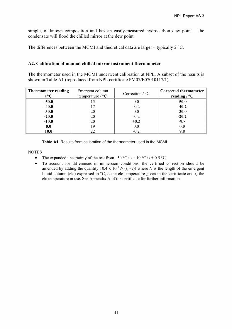
simple, of known composition and has an easily-measured hydrocarbon dew point – the condensate will flood the chilled mirror at the dew point. The differences between the MCMI and theoretical data are larger – typically 2 °C. A2. Calibration of manual chilled mirror instrument thermometer The thermometer used in the MCMI underwent calibration at NPL. A subset of the results is shown in Table A1 (reproduced from NPL certificate PM07/E07010117/1). Thermometer reading
/ °C Emergent column temperature / °C Correction / °C Corrected thermometer
reading / °C -50.0 15 0.0 -50.0 -40.0 17 -0.2 -40.2 -30.0 20 0.0 -30.0 -20.0 20 -0.2 -20.2 -10.0 20 +0.2 -9.8 0.0 19 0.0 0.0
10.0 22 -0.2 9.8
Table A1. Results from calibration of the thermometer used in the MCMI. NOTES
• The expanded uncertainty of the test from –50 °C to + 10 °C is ± 0.5 °C. • To account for differences in immersion conditions, the certified correction should be
amended by adding the quantity 10.4 x 10⁻⁴ N (t1 - t2) where N is the length of the emergent liquid column (elc) expressed in °C, t1 the elc temperature given in the certificate and t2 the elc temperature in use. See Appendix A of the certificate for further information.

NPL Report AS 3
42
ANNEX B – CALCULATION OF DEW CURVES FOR WATER VAPOUR In order to investigate an example of the retrograde behaviour of a water dewline calculated using the RKS equation of state in an earlier version of this report, five methods of calculation were compared, namely:
• LRS • PR • ISOW (modified PR equation of state for the calculation of water dew point according
to ISO 18453 [13]) • RKS with Kij
= 0 (full composition) – the default option for the software used • RKS with Kij = 0.5 (full composition) • RKS with Kij = 0.5 (simplified composition)
Gas A was used in the calculation, its composition taken from the Lab GC 1 analysis (for all species except water), with the water content calculated to achieve the National Grid National Transmission System indicative specification of a water dew point of –10 °C at 85 bar. (The actual amount fraction of water therefore differed slightly between each equation of state). The ‘simplified composition’ assumes that all hydrocarbons from C2 to C12 could be represented by C2, and that N2, O2, He and H2 could be represented by N2.
Comparison of water dewcurves
0
20
40
60
80
100
-40 -30 -20 -10 0
Temperature (C)
Pres
sure
(bar
)
LRSPRISOWRKS (Kij = 0.5; full comp)RKS (Kij = 0.5; simplif ied comp)RKS (Kij = 0; full comp)
Figure B1. Comparison of water dewlines plotted using different equations of state. Note that all the curves converge at a pressure of 85 bar due to the use of the NTS indicative water specification
The results (Figure B1) show that the use of an RKS equation of state with Kij = 0 would clearly be an erroneous approach – the curve shows retrograde behaviour which is uncharacteristic of a water dew curve. The two RKS (Kij = 0.5) curves show good agreement, but a large difference is shown by the ISOW curve. This is due to the phase of the condensed water in the equation – the LRS, PR & RKS EoS assumes water to be in the liquid phase, but the ISOW EoS gives the condensed phase of water below 0°C as ice (i.e. in the solid phase).

NP
L R
epor
t AS
3
43
AN
NE
X C
– C
OM
POSI
TIO
N O
F V
APO
UR
AN
D L
IQU
ID P
HA
SES
OF
SYN
TH
ET
IC M
IXT
UR
ES
OF
NA
TU
RA
L G
AS
Vap
our p
hase
am
ount
frac
tion
- Hig
h
020406080100
02
46
810
Tem
pera
ture
bel
ow c
ricon
dent
herm
/ de
g C
Amount fraction in vap phase (as % of grav. am. fract.)
C1 C2 C3 n-C4
n-C5
n-C6
Benz
ene
Tolu
ene
Cyc-
C6n-
C7n-
C8n-
C9n-
C10
Liqu
id p
hase
am
ount
frac
tion
- Hig
h
0
2000
00
4000
00
6000
00
8000
00
1000
000
1200
000
1400
000
1600
000
1800
000
02
46
810
Tem
pera
ture
bel
ow c
ricon
dent
herm
/ de
g C
Amount fraction in liq phase (as % of grav. am. fract.)
C1 C2 C3 n-C4
n-C5
n-C6
Benz
ene
Tolu
ene
Cyc-
C6n-
C7n-
C8n-
C9n-
C10
Va
pour
pha
se a
mou
nt fr
actio
n - H
igh
-8-7-6-5-4-3-2-1012
02
46
810
Tem
pera
ture
bel
ow c
ricon
dent
herm
/ de
g C
log (amount fraction)[vapour phase]
C1 C2 C3 n-C4
n-C5
n-C6
Benz
ene
Tolu
ene
Cyc-
C6n-
C7n-
C8n-
C9n-
C10
Liqu
id p
hase
am
ount
frac
tion
- Hig
h
-4-3-2-1012
02
46
810
Tem
pera
ture
bel
ow c
ricon
dent
herm
/ de
g C
log (amount fraction)[liquid phase]
C1 C2 C3 n-C4
n-C5
n-C6
Benz
ene
Tolu
ene
Cyc-
C6n-
C7n-
C8n-
C9n-
C10
Fi
gure
C1.
Com
paris
on o
f liq
uid
and
vapo
ur p
hase
s of
mix
ture
Hig
h at
tem
pera
ture
s be
low
the
cric
onde
nthe
rm. N
ote
that
: n-C
9 an
d n-
C10
are
pre
sent
in th
e m
ixtu
re a
s an
impu
rity
only
.
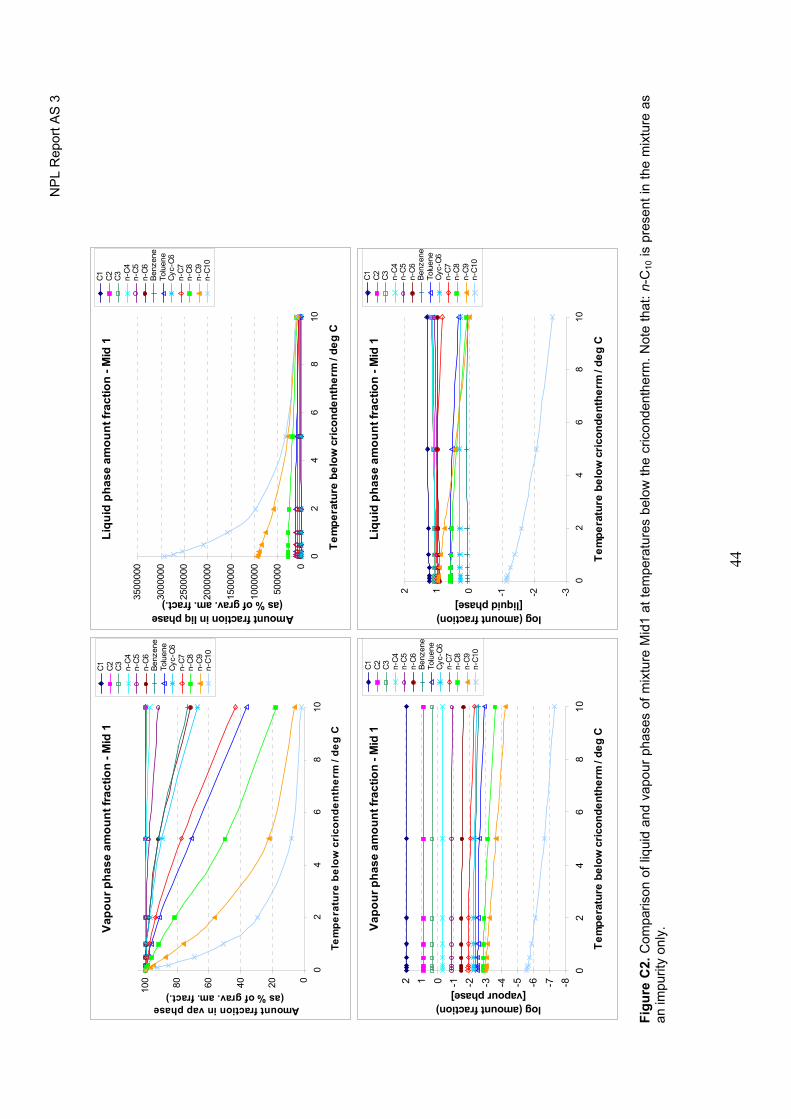
NP
L R
epor
t AS
3
44
Vap
our p
hase
am
ount
frac
tion
- Mid
1
020406080100
02
46
810
Tem
pera
ture
bel
ow c
rico
nden
ther
m /
deg
C
Amount fraction in vap phase (as % of grav. am. fract.)
C1 C2 C3 n-C4
n-C5
n-C6
Benz
ene
Tolu
ene
Cyc-
C6n-
C7n-
C8n-
C9n-
C10
Liqu
id p
hase
am
ount
frac
tion
- Mid
1
0
5000
00
1000
000
1500
000
2000
000
2500
000
3000
000
3500
000
02
46
810
Tem
pera
ture
bel
ow c
ricon
dent
herm
/ de
g C
Amount fraction in liq phase (as % of grav. am. fract.)
C1 C2 C3 n-C4
n-C5
n-C6
Benz
ene
Tolu
ene
Cyc-
C6n-
C7n-
C8n-
C9n-
C10
Va
pour
pha
se a
mou
nt fr
actio
n - M
id 1
-8-7-6-5-4-3-2-1012
02
46
810
Tem
pera
ture
bel
ow c
ricon
dent
herm
/ de
g C
log (amount fraction) [vapour phase]
C1 C2 C3 n-C4
n-C5
n-C6
Benz
ene
Tolu
ene
Cyc-
C6n-
C7n-
C8n-
C9n-
C10
Liqu
id p
hase
am
ount
frac
tion
- Mid
1
-3-2-1012
02
46
810
Tem
pera
ture
bel
ow c
ricon
dent
herm
/ de
g C
log (amount fraction) [liquid phase]
C1 C2 C3 n-C4
n-C5
n-C6
Benz
ene
Tolu
ene
Cyc-
C6n-
C7n-
C8n-
C9n-
C10
Fi
gure
C2.
Com
paris
on o
f liq
uid
and
vapo
ur p
hase
s of
mix
ture
Mid
1 at
tem
pera
ture
s be
low
the
cric
onde
nthe
rm. N
ote
that
: n-C
10 is
pre
sent
in th
e m
ixtu
re a
s an
impu
rity
only
.

NP
L R
epor
t AS
3
45
Vapo
ur p
hase
am
ount
frac
tion
- Mid
2
020406080100
02
46
810
Tem
pera
ture
bel
ow c
ricon
dent
herm
/ de
g C
Amount fraction in vap phase (as % of grav. am. fract.)
C1 C2 C3 n-C4
n-C5
n-C6
Benz
ene
Tolu
ene
Cyc-
C6n-
C7n-
C8n-
C9n-
C10
Liqu
id p
hase
am
ount
frac
tion
- Mid
2
0
5000
00
1000
000
1500
000
2000
000
2500
000
3000
000
02
46
810
Tem
pera
ture
bel
ow c
ricon
dent
herm
/ de
g C
Amount fraction in liq phase (as % of grav. am. fract.)
C1 C2 C3 n-C4
n-C5
n-C6
Benz
ene
Tolu
ene
Cyc-
C6n-
C7n-
C8n-
C9n-
C10
Vap
our p
hase
am
ount
frac
tion
- Mid
2
-8-7-6-5-4-3-2-1012
02
46
810
Tem
pera
ture
bel
ow c
ricon
dent
herm
/ de
g C
log (amount fraction) [vapour phase]
C1 C2 C3 n-C4
n-C5
n-C6
Benz
ene
Tolu
ene
Cyc-
C6n-
C7n-
C8n-
C9n-
C10
Liqu
id p
hase
am
ount
frac
tion
- Mid
2
-3-2-1012
02
46
810
Tem
pera
ture
bel
ow c
ricon
dent
herm
/ de
g C
log (amount fraction) [liquid phase]
C1 C2 C3 n-C4
n-C5
n-C6
Benz
ene
Tolu
ene
Cyc-
C6n-
C7n-
C8n-
C9n-
C10
Fi
gure
C3.
Com
paris
on o
f liq
uid
and
vapo
ur p
hase
s of
mix
ture
Mid
2 a
t tem
pera
ture
s be
low
the
cric
onde
nthe
rm. N
ote
that
: n-C
10 is
pre
sent
in th
e m
ixtu
re a
s an
impu
rity
only
.

NP
L R
epor
t AS
3
46
Vapo
ur p
hase
am
ount
frac
tion
- Low
1
020406080100
02
46
810
Tem
pera
ture
bel
ow c
ricon
dent
herm
/ de
g C
Amount fraction in vap phase (as % of grav. am. fract.)
C1 C2 C3 n-C4
n-C5
n-C6
Benz
ene
Tolu
ene
Cyc-
C6n-
C7n-
C8n-
C9n-
C10
Liqu
id p
hase
am
ount
frac
tion
- Low
1
0
5000
00
1000
000
1500
000
2000
000
2500
000
3000
000
3500
000
4000
000
02
46
810
Tem
pera
ture
bel
ow c
ricon
dent
herm
/ de
g C
Amount fraction in liq phase (as % of grav. am. fract.)
C1 C2 C3 n-C4
n-C5
n-C6
Benz
ene
Tolu
ene
Cyc-
C6n-
C7n-
C8n-
C9n-
C10
Va
pour
pha
se a
mou
nt fr
actio
n - L
ow 1
-4-3-2-1012
02
46
810
Tem
pera
ture
bel
ow c
ricon
dent
herm
/ de
g C
log (amount fraction) [vapour phase]
C1 C2 C3 n-C4
n-C5
n-C6
Benz
ene
Tolu
ene
Cyc-
C6n-
C7n-
C8n-
C9n-
C10
Liqu
id p
hase
am
ount
frac
tion
- Low
1
-0.50
0.51
1.52
02
46
810
Tem
pera
ture
bel
ow c
ricon
dent
herm
/ de
g C
log (amount fraction) [liquid phase]
C1 C2 C3 n-C4
n-C5
n-C6
Benz
ene
Tolu
ene
Cyc-
C6n-
C7n-
C8n-
C9n-
C10
Fi
gure
C4.
Com
paris
on o
f liq
uid
and
vapo
ur p
hase
s of
mix
ture
Low
1 a
t tem
pera
ture
s be
low
the
cric
onde
nthe
rm

NP
L R
epor
t AS
3
47
Vapo
ur p
hase
am
ount
frac
tion
- Low
2
020406080100
02
46
810
Tem
pera
ture
bel
ow c
ricon
dent
herm
/ de
g C
Amount fraction in vap phase (as % of grav. am. fract.)
C1 C2 C3 n-C4
n-C5
n-C6
Benz
ene
Tolu
ene
Cyc-
C6n-
C7n-
C8n-
C9n-
C10
Liqu
id p
hase
am
ount
frac
tion
- Low
2
0
5000
00
1000
000
1500
000
2000
000
2500
000
3000
000
02
46
810
Tem
pera
ture
bel
ow c
ricon
dent
herm
/ de
g C
Amount fraction in liq phase (as % of grav. am. fract.)
C1 C2 C3 n-C4
n-C5
n-C6
Benz
ene
Tolu
ene
Cyc-
C6n-
C7n-
C8n-
C9n-
C10
Va
pour
pha
se a
mou
nt fr
actio
n - L
ow 2
-4-3-2-1012
02
46
810
Tem
pera
ture
bel
ow c
ricon
dent
herm
/ de
g C
log (amount fraction) [vapour phase]
C1 C2 C3 n-C4
n-C5
n-C6
Benz
ene
Tolu
ene
Cyc-
C6n-
C7n-
C8n-
C9n-
C10
Liqu
id p
hase
am
ount
frac
tion
- Low
2
-0.50
0.51
1.52
02
46
810
Tem
pera
ture
bel
ow c
ricon
dent
herm
/ de
g C
log (amount fraction) [liquid phase]
C1 C2 C3 n-C4
n-C5
n-C6
Benz
ene
Tolu
ene
Cyc-
C6n-
C7n-
C8n-
C9n-
C10
Fi
gure
C5.
Com
paris
on o
f liq
uid
and
vapo
ur p
hase
s of
mix
ture
Low
2 a
t tem
pera
ture
s be
low
the
cric
onde
nthe
rm