NPCirc: An R Package for Nonparametric Circular Methods

JSS Journal of Statistical SoftwareOctober 2014, Volume 61, Issue 9. http://www.jstatsoft.org/

NPCirc: An R Package for Nonparametric Circular

Methods

Marıa OliveiraUniversity of Santiago

de Compostela

Rosa M. CrujeirasUniversity of Santiago

de Compostela

Alberto Rodrıguez-CasalUniversity of Santiago

de Compostela

Abstract

Nonparametric density and regression estimation methods for circular data are in-cluded in the R package NPCirc. Specifically, a circular kernel density estimation proce-dure is provided, jointly with different alternatives for choosing the smoothing parameter.In the regression setting, nonparametric estimation for circular-linear, circular-circular andlinear-circular data is also possible via the adaptation of the classical Nadaraya-Watsonand local linear estimators. In order to assess the significance of the features observed inthe smooth curves, both for density and regression with a circular covariate and a linearresponse, a SiZer technique is developed for circular data, namely CircSiZer. Some dataexamples are also included in the package, jointly with a routine that allows generatingmixtures of different circular distributions.

Keywords: circular data, CircSiZer, nonparametric methods, mixtures, R package.

1. Introduction

Statistical methods for circular data analysis have turned out to be the appropriate tools inmany applied fields, such as biology (Batschelet 1981), ecology (Jammalamadaka and Lund2006), meteorology (Bowers, Morton, and Mould 2000), sociology (Brunsdon and Corcoran2005), medicine (Mooney, Helms, and Jollife 2003) or biomechanics (Mann, Gupta, Race,Miller, and Cleary 2003), among others. From a methodological perspective, most of theseapplied papers make use of circular descriptive techniques, providing graphical displays ofthe data such as rose diagrams, and in some cases, classical parametric inferential tools areconsidered, with the von Mises distribution being a cornerstone in this approach.

Modeling circular data distributions by means of parametric families has been covered inmost of the papers in the statistical literature. Comprehensive reviews such as Mardia (1972),

http://www.jstatsoft.org/

2 NPCirc: Nonparametric Circular Methods in R

Fisher (1993), Jammalamadaka and SenGupta (2001) and Mardia and Jupp (2000) presentparametric models such as the aforementioned von Mises, the cardiod, or the wrapped-normaldistributions, among others, jointly with testing procedures for assessing uniformity, suchas Rayleigh’s, Kuiper’s, Rao’s spacing or Watson’s tests. Although being widely used, thevon Mises model is not flexible enough to capture the underlying structure of multimodal,highly peaked or skewed distributions. Some new parametric models for handling these fea-tures have been presented by Abe and Pewsey (2011), who introduced circular models withtwo diametrically opposed modes, or Jones and Pewsey (2012), who proposed the inverseBatschelet distribution, accounting for skewness and high kurtosis. The consideration ofmixtures of parametric models may offer a route to capture complex structures, but at thecost of increasing the number of parameters characterizing the distribution. In this settingparametric estimation can be done by maximum likelihood arguments using the expectation-maximization (EM) framework as in Banerjee, Dhillon, Ghosh, and Sra (2005), and model fitcan be approached by means of an information criterion. Nevertheless, the specification of anappropriate parametric family may not be an easy task.

Nonparametric estimation methods have turned up as an alternative approach, both infer-entially and as a descriptive tool. Specifically, a kernel density estimation procedure wasproposed by Hall, Watson, and Cabrera (1987), for the general case of spherical data, follow-ing the ideas of the classical kernel density estimator for linear data (Parzen 1962; Rosenblatt1956). Although asymptotic properties of this estimator were further studied by Bai, Rao,and Zhao (1988) and Klemela (2000), these latter works do not provide a solution for themost critical issue from a practical point of view: smoothing parameter selection. The useof cross-validation smoothing parameters is suggested by Hall et al. (1987), in the sphericalcontext, and for the particular case of circular data, Taylor (2008) derived a rule of thumbfor smoothing parameter selection in circular kernel density estimation. Despite being asimple procedure, the performance of this rule is extremely poor in some distribution set-tings involving multimodality, peakedness or skewness, as shown by Oliveira, Crujeiras, andRodrıguez-Casal (2012). Marzio, Panzera, and Taylor (2011) introduced a bootstrap methodwith the same purpose, but with unsatisfactory results for small data samples. Recently,Oliveira et al. (2012) devised a new procedure for selecting the smoothing parameter in cir-cular kernel density estimation that performs well in distributional scenarios beyond the vonMises case, and presents better or at least competitive results compared with the previouslyproposed selectors.

Regression estimation involving circular variables, as a response or as a covariate, is indeedan interesting problem. In the available literature, most efforts have been focused on thedevelopment of parametric models. For instance, Presnell, Morrison, and Littel (1998) andthe references therein dealt with a circular response and linear covariates; SenGupta andUgwuowo (2006) proposed some asymmetric models accounting for the circular nature ofthe covariate and Downs and Mardia (2002) and Kato, Shimizu, and Shieh (2008), amongothers, addressed the regression with circular response and covariates. Regression estimationavoiding the assumption of a specific parametric shape for the regression curve was studiedby Marzio, Panzera, and Taylor (2009) who extended the least squares local polynomial tothe case of d-dimensional circular predictors and real-valued responses; Qin, Zhang, and Yan(2011a,b) extended nonparametric models to the case when there is one circular predictorand one or more linear predictors and the response is real-valued, and more recently Marzio,Panzera, and Taylor (2012) proposed a nonparametric estimator for the regression function

Journal of Statistical Software 3

when the response is circular and the covariate is circular or linear. In the regression setting,the smoothing parameter can be chosen by cross-validation methods.

Both for density and regression estimation, the smoothing parameter controls the global ap-pearance of the estimator and its dependence on the sample, and it is well-known that anunsuitable choice of this value may provide a misleading estimate of the density or the re-gression curve. Hence, the assessment of the statistical significance of the observed featuresthrough the smoothed curve may be seriously compromised if an undersmoothed or an over-smoothed estimator is produced. An alternative to circumvent the choice of the smoothingparameter, and still be able to assess global structure features in the curve, is given by theSiZer (significative zero crossing of the derivative) method developed by Chaudhuri and Mar-ron (1999) for the analysis of linear data. The idea behind this technique is to determinethe regions of significant gradients (zero crossing of the derivative) over a range of smooth-ing values. The SiZer ideas have been adapted to the circular setting, both for density andcircular-linear regression, as proposed by Oliveira, Crujeiras, and Rodrıguez-Casal (2014a),by means of the CircSiZer map.

Package NPCirc (Oliveira, Crujeiras, and Rodrıguez-Casal 2014b) described in this paper isintended to provide R (R Core Team 2014) users with a comprehensive set of functions fornonparametric density and regression analysis with circular data. There are other packagesfor working with circular data, already available in R but, at the best of our knowledge, noneof them is devoted to nonparametric methods. Some useful references to work in R withcircular data are:

� CircStats (Lund and Agostinelli 2012): This package provides methods for the descrip-tive and inferential statistical analysis of directional data. It is based on the book“Topics in Circular Statistics” by Jammalamadaka and SenGupta (2001). Functionsimplemented in this package are also available in the circular package.

� circular (Lund and Agostinelli 2013): An extension of the CircStats package, circularprovides functions for the statistical analysis (descriptive statistics, circular models,tests), graphical representation and some circular datasets.

� CircNNTSR (Fernandez-Duran and Gregorio-Domınguez 2013): Functions for con-structing circular distributions based on nonnegative trigonometric sums, estimatingparameters and plotting the constructed densities, are included herein.

� isocir (Barragan and Fernandez 2014): This package provides a set of routines foranalyzing angular data subjected to order constraints on a unit circle.

� movMF (Hornik and Grun 2014): Focused on mixtures of von Mises distributions,this package allows to draw random samples from these models and to proceed withparameter estimation, by using an EM algorithm.

A specific function for kernel density estimation for circular data, and three functions forsmoothing parameter selection, have been already included in package circular. These selec-tors are the cross-validation rules proposed by Hall et al. (1987) and the rule of thumb intro-duced by Taylor (2008). Apart from this, there is no other function for nonparametric regres-sion estimation and smoothing parameter selection available. From the parametric perspec-tive, packages circular, CircStats and movMF allow to compute the density function and do


random generation of mixtures of von Mises distributions but, it is not possible to do the samewith mixtures of different circular distributions. Hence, the functions in NPCirc will comple-ment other implementations of circular data analysis in three ways. Firstly, in this package,the circular kernel density estimator with an up-to-date collection of smoothing parameterselection procedures are included; Nadaraya-Watson and local linear estimators for circular-linear, linear-circular and circular-circular data, with the corresponding least squares cross-validations rule for smoothing choice, have been also implemented. Secondly, CircSiZer mapsfor density and regression for a circular covariate and a linear response can be also obtained.Finally, NPCirc contains functions for generating data and obtaining densities of a variety ofcircular models, and mixtures of them. Specifically, the collection of circular models presentedin Oliveira et al. (2012), can be directly generated. The package is available from the Com-prehensive R Archive Network (CRAN) at http://CRAN.R-project.org/package=NPCirc.

The structure of this paper is as follows. Section 2 provides a brief overview on kernel densityestimation for circular data, and regression estimation involving circular variables, revisingdifferent smoothing parameter selection procedures in both settings. The CircSiZer map isalso briefly described here. In Section 3, usage of functions and datasets in the package aredescribed and illustrated. Finally, some remarks are given in Section 4, discussing furtherextensions of the package.

2. Nonparametric circular methods

As mentioned in Section 1, classical parametric circular models may not be flexible enough tocapture complex data distributions, and it is in this scenario where nonparametric methodsplay an important role. Nevertheless, before presenting the circular kernel density estimatorand, in order to understand its construction, the von Mises distribution and mixtures ofcircular distributions are introduced.

The von Mises distribution, vM (µ, κ) (von Mises 1918) is a symmetric unimodal distributioncharacterized by a mean direction µ ∈ [0, 2π), and a concentration parameter κ ≥ 0, withprobability density function

f(θ;µ, κ) =1

2πI0(κ)exp {κ cos(θ − µ)} , 0 ≤ θ < 2π, (1)

where Ir(κ) denotes the modified Bessel function of order r (see Jammalamadaka and Sen-Gupta 2001, Section 2.2.4). The mean direction coincides with the mode, whereas the pa-rameter κ measures the concentration around the mean direction µ in such a way that, asκ increases, the density peaks higher around µ. As commented before, most of the classicalparametric models are unimodal and symmetric (e.g., von Mises, cardioid, wrapped normal,wrapped Cauchy, . . . ), except for the wrapped skew-normal (Pewsey 2000) which is asym-metric.

More flexible models, allowing for multimodality and/or asymmetry, can be obtained bymixing a finite number M of circular distributions fm, m = 1, . . . ,M , with density

f(θ) =M∑m=1

pmfm(θ), withM∑m=1

pm = 1, (2)

where pm > 0 is the proportion of the density fm in the mixture. Although mixture modelsare useful for constructing distributions that may exhibit complex shapes, this is done at

http://CRAN.R-project.org/package=NPCirc


the cost of including a possibly large number of parameters, usually estimated by maximumlikelihood arguments. In addition, the selection of the number of density components in themixture is another problem, that may be approached by considering some kind of informationcriterion such as the Akaike information criterion (AIC).

Next, the circular kernel density estimator will be briefly described, jointly with an overviewof the smoothing parameter selection methods that are included in the NPCirc package.

2.1. Circular kernel density estimation

Given a random sample of angles Θ1,Θ2, . . . ,Θn ∈ [0, 2π) from some unknown circular densityf , the circular kernel density estimator of f is defined as:

f(θ; ν) =1

n

n∑i=1

Kν(θ −Θi), 0 ≤ θ < 2π,

where Kν is a circular kernel function with concentration ν > 0 (Marzio et al. 2009), beingthe smoothness of the estimated curve controlled by this parameter. As a circular kernel, thevon Mises distribution vM (0, ν) (see Equation 1) can be considered. With this specific kernel,the density estimator is given by:

f(θ; ν) =1

2nπI0(ν)

n∑i=1

exp {ν cos(θ −Θi)}, 0 ≤ θ < 2π. (3)

Hence, the estimator can be interpreted as a mixture of n random variables with von Misesdistribution, centered in the sample points Θi and with common concentration parameter ν.A critical issue is the choice of the smoothing parameter ν for Equation 3, with large valuesleading to highly variable (undersmoothed) estimators and small values showing an oppositebehavior (oversmoothed curve).

The smoothing parameter is usually selected in order to minimize some error criterion, suchas the mean integrated squared error (MISE, MISE(ν) = E(

∫(f−f)2)). The closed expression

for the asymptotic MISE (AMISE) of the circular kernel density estimator has been derivedby Marzio et al. (2009). When ν →∞ and

√νn−1 → 0, the AMISE(ν) is given by:

AMISE(ν) =

{1

16

[1− I2(ν)

I0(ν)

]2 ∫ 2π

0

[f ′′(θ)

]2dθ +

I0(2ν)

2nπ (I0(ν))2

}, (4)

where f ′′ denotes the second-order derivative of the target density to be estimated, whichmeasures the curvature of f .

The proposal presented by Taylor (2008) for selecting the smoothing parameter is based onthe assumption that the data follow a von Mises distribution with concentration parameterκ. In this case, the AMISE expression simplifies and the value of the optimal smoothingparameter, that minimizes AMISE, can be estimated by:

νRT =

[3nκ2I2(2κ)

4π1/2I0(κ)2

]2/5, (5)

where κ is obtained by maximum likelihood estimation. This selector performs satisfactorilyin fitting unimodal symmetric distributions, without highly peaked modes but its behavior can


be dramatically misleading in the presence of antipodal modes and/or skewed distributions,as shown by Oliveira et al. (2012). The poor performance is sometimes due to the non-robust estimation by maximum likelihood of the concentration parameter κ, so a modificationof Equation 5 described in Oliveira, Crujeiras, and Rodrıguez-Casal (2013) consists of thefollowing procedure:

Step 1. Select α ∈ (0, 1) and find the shortest arc containing α · 100% of the sample data.

Step 2. Obtain the estimated κ in such way that∫f(θ, µarc, κ)dθ = α where µarc is the

midpoint of the arc computed in Step 1. The integral is computed over the arcselected in Step 1.

Also based on the AMISE minimization, an alternative route to get a smoothing parametervalue would be to plug-in as reference density a more flexible distribution, instead of thevon Mises model taken by Taylor (2008). For that purpose, a mixture of M von Misesdistributions, vM (µi, κi) with proportions pm > 0, m = 1, . . . ,M can be considered:

g(θ) =M∑m=1

pmexp {κm cos(θ − µm)}

2πI0(κm), with

M∑m=1

pm = 1. (6)

In that case, the proposed plug-in smoothing parameter selector, νPI , is obtained as follows(see Oliveira et al. 2012, for further details):

Step 1. Based on the sample information, select the number of mixture components M forthe reference distribution.

Step 2. Estimate the parameters in the von Mises mixture (Equation 6), (µm, κm, pm), form = 1, . . . ,M and compute the integral

∫(g′′(θ))2dθ. plug-in this quantity in the

AMISE expression (Equation 4) to get AMISE(ν).

Step 3. Minimize AMISE(ν) and obtain νPI .

In Step 1, the selection of the number of mixture components in the reference distribution canbe done by AIC, considering different numbers of mixture components, namely M . Maximumlikelihood estimation via the EM algorithm (Banerjee et al. 2005) is used in Step 2. In Step 3,an optimization method can be implemented, in order to minimize the AMISE.

Cross-validation rules, as the ones proposed by Hall et al. (1987), are also an alternativefor smoothing parameter selection in circular data problems. The likelihood cross-validationsmoothing parameter νLCV is obtained by maximizing:

LCV(ν) =n∏i=1

f−i(Θi; ν), (7)

where f−i denotes the circular kernel density estimator (Equation 3) leaving out the ithobservation. The least squares cross-validation smoothing parameter is obtained as the valueνLSCV that minimizes:

LSCV(ν) =

∫ 2π

0f2(θ; ν)dθ − 2

n

n∑i=1

f−i(Θi; ν). (8)


Oliveira et al. (2012) showed that νLCV provides reasonable results except for highly peakeddistributions and, in general, it is more stable that νLSCV.

Finally, Marzio et al. (2011) introduced a bootstrap method for choosing the smoothingparameter. The idea is to take the value that minimizes the bootstrap version of MISE,which has a closed expression when the von Mises kernel is used. The main drawback of thismethod is that the function to minimize has a global minimum at ν = 0 leading to a uniformcircular estimate, regardless of the true underlying model. In practice, this will lead to asearch for a local minimum, which may pose a problem especially for small samples.

2.2. Circular kernel regression estimation

Kernel regression estimation with circular response and/or covariate are revised in this section.

Nonparametric regression for a circular covariate and a linear response

Let {(Θi, Yi), i = 1, . . . , n} denote a random sample from (Θ, Y ) a circular and a linear ran-dom variable, respectively. The relation between these variables may be explained by aregression model such as

Yi = f(Θi) + εi, i = 1, . . . , n, (9)

where f denotes now the regression function and εi are real-valued random variables withzero mean and variance σ2 and independent of the Θis. The local circular-linear regressionestimates for f(θ) and f ′(θ) are given by f(θ; ν) = a and f ′(θ; ν) = b, where

(a, b) = arg min(a,b)

n∑i=1

Kν(θ −Θi) [Yi − (a+ b sin(Θi − θ))]2 (10)

(see Marzio et al. 2009, for further details). As for density estimation, in Equation 10,ν > 0 is the smoothing parameter and Kν is a circular kernel function with concentration ν.Usually, a von Mises kernel with concentration parameter ν is considered. If the regressionfunction is locally approximated by a constant instead of using a trigonometric polynomial,the Nadaraya-Watson estimator for circular-linear data is obtained:

fCNW(θ; ν) =

∑ni=1 YiKν(θ −Θi)∑ni=1Kν(θ −Θi)

. (11)

For both Equations 10 and 11, the smoothing parameter ν controls the degree of smoothing.Large values of ν lead to undersmoothed estimations of the regression curve, tending to aninterpolation of the data. On the other hand, small values of ν result in a global averaging,oversmoothing the local features in the data. A simple and widely used procedure for smooth-ing parameter selection in the regression setting is least squares cross-validation, choosing νas the value minimizing:

CV(ν) =1

n

n∑i=1

[Yi − f−i(Θi)

]2, (12)

where f−i is the leave-one-out estimator for the regression function, for i = 1, . . . , n. This willbe the method implemented in NPCirc for selecting the smoothing parameter in regressionfitting, both for local linear and Nadaraya-Watson estimators.


Nonparametric regression for a circular response

Let {(∆i,Φi), i = 1, . . . , n} denote a random sample from (∆,Φ), where Φ is a circular randomvariable and ∆ will denote a linear or circular random variable. Following Marzio et al. (2012),the relation between these variables may be explained by a regression model such as

Φi = [f(∆i) + εi] (mod2π), i = 1, . . . , n,

where the random angles εi have zero mean direction, finite concentration, and are indepen-dent of the ∆is.

A nonparametric estimator of the regression function f at a point δ (which may be real orcircular) can be written as,

f(δ) = atan2 [g1(δ), g2(δ)] ,

where the function atan2 [y, x] returns the angle between the x-axis and the vector from theorigin to (x, y) and

g1(δ) =1

n

n∑i=1

sin(Φi)W (∆i − δ) and g2(δ) =1

n

n∑i=1

cos(Φi)W (∆i − δ)

with W being a local weight.

Following Marzio et al. (2012), both for a circular or a linear covariate, kernel weights and locallinear weights can be considered yielding the Nadaraya-Watson and local linear estimators,respectively. For the case of a circular covariate, the kernel weights are given by taking acircular kernel as weight function and the local linear weights are given by

W (∆i − δ) = n−1Kν(∆i − δ)

n∑j=1

Kν(∆j − δ) sin2(∆j − δ)

− sin(∆i − δ)n∑j=1

Kν(∆j − δ) sin(∆j − δ)

,where Kν denotes a circular kernel and ν is the smoothing parameter. For the case of a linearcovariate, the kernel weights are given by taking a linear kernel as weight function and thelocal linear weights are given by

W (∆i−δ) = n−1Kh(∆i−δ)

n∑j=1

Kh(∆j − δ)(∆j − δ)2 − (∆i − δ)n∑j=1

Kh(∆j − δ)(∆j − δ)

,where Kh denotes a linear kernel and h is the smoothing parameter. By default, kernelsin NPCirc are von Mises distributions vM (0, ν) for the circular case and N(0, h2) for linearvariables.

In both cases, circular or linear covariate, a smoothing parameter (ν or h) must be chosenwhich may be selected by minimizing one of the following cross-validation functions:

CV(τ) = −n∑i=1

cos(Φi − f−i(∆i)

), (13)


CV(τ) =1

n

n∑i=1

d2(Φi, f−i(∆i)

), (14)

where τ denotes the smoothing parameter (ν or h depending on the case) and d(Φi, f−i(∆i)

)=

min(|Φi − f−i(∆i)|, 2π − |Φi − f−i(∆i)|). By default, the first option will be the method im-plemented in NPCirc for selecting the smoothing parameter.

2.3. CircSiZer map

From a practical perspective, the concerns about the requirement of an appropriate smooth-ing value for constructing a density or regression estimator may discourage the use of theaforementioned kernel techniques. Indeed, exploring the estimators at different smoothinglevels, by trying a reasonable range between oversmoothing and undersmoothing, will pro-vide a thorough perception of the data structure. This idea may be seen as directly feasibleby constructing such estimators, but significance of the observed features in the smoothedcurve, like peaks and valleys, must be statistically assessed. As proposed by Chaudhuri andMarron (1999), this can be done by studying the zero crossings of the derivative, providingthe SiZer map for linear data, and this procedure has been adapted to the circular frameworkby Oliveira et al. (2014a), via the CircSiZer map included in NPCirc, both for density andcircular-linear regression.

In order to assess the statistical significance of features such as peaks and valleys, CircSiZerseeks confidence intervals for the scale-space version f ′(θ; ν) ≡ E(f ′(θ; ν)), where f is thedensity or the regression function. A possible way to get such intervals is by means of the“bootstrap t” approach, as detailed in Oliveira et al. (2014a). The output of this procedureis a graphical display, the CircSiZer map, which reflects the statistical significance of f ′(θ, ν)with θ ∈ [0, 2π) and ν varying along a range of values. The CircSiZer map is a circular colorplot where the performance of the estimated curve for each given value of the smoothingparameter ν is represented by a color ring, in such way that the different colors will allow toidentify peaks and valleys. The construction is as follow: for each pair (θ, ν), the curve ata smoothing level ν is significantly increasing (decreasing) if the confidence interval is above(below) 0, so that the corresponding map location is colored blue (red). If the confidenceinterval contains 0, the curve at the smoothing level ν and at the angle θ does not present astatistically significant slope and it is colored in purple. Regions where there are not enoughdata to make statements about significance are gray colored. Gray locations are determinedaccording to the estimated effective sample size (see Oliveira et al. 2014a, for details in itscalculus). The appearance of the CircSiZer map will be clear in the examples presented inthe next section.

3. NPCirc package

In this section, a detailed description of NPCirc’s capabilities is provided. The complete listof functions and datasets available in NPCirc, with a brief explanation of each of them, canbe seen in Table 1. First, some comments will be made about the datasets included in thepackage. Functions related to mixture circular models generation and circular kernel densityestimation will be described later. Finally, usage of functions for circular-linear, circular-circular and linear-circular regression will be commented. Both for density and circular-linear


Dataset Description

cross.beds1 Cross-beds azimuths (I)cross.beds2 Cross-beds (II)cycle.changes Cycle changesdragonfly Orientation of dragonfliesperiwinkles Snail movements dataspeed.wind, speed.wind2 Wind speed and wind direction datatemp.wind Temperature and wind direction datawind Wind direction data

Function Description

circsizer.density CircSiZer for densitycircsizer.regression CircSiZer for regressioncircsizer.map Plot a CircSiZer mapdwsn Density function of a wrapped skew-normal distributionrwsn Random generation from a wrapped skew-normal

distributiondcircmix Density function of mixtures of circular distributionsrcircmix Random generation from mixtures of circular

distributionskern.den.circ Nonparametric circular kernel density estimationkern.reg.circ.lin Nonparametric circular-linear regressionkern.reg.circ.circ Nonparametric circular-circular regressionkern.reg.lin.circ Nonparametric linear-circular regressionbw.CV Cross-validation for density estimationbw.boot Bootstrap methodbw.pi Plug-in rulebw.rt Rule of thumbbw.reg.circ.lin Cross-validation for circular-linear regressionbw.reg.circ.circ Cross-validation for circular-circular regressionbw.reg.lin.circ Cross-validation for linear-circular regressionS3 plot method for Plot circular regression‘regression.circular’ objectsS3 lines method for Add a plot for circular regression‘regression.circular’ objects

Table 1: Summary of NPCirc package contents.

regression estimation, functions for obtaining the CircSiZer maps will be also presented.

3.1. Data description

NPCirc includes some classical datasets, as those ones collecting cross-beds angles or ani-mal orientation data, and some original ones, on temperature and wind data measurements.Specifically, the dataset cross.beds1 corresponds to azimuths of cross-beds in the Kamthiriver (India). Originally analyzed by SenGupta and Rao (1966) and included in Table 1.5in Mardia (1972), the dataset collects 580 azimuths of layers lying oblique to principal ac-cumulation surface along the river, these layers being known as cross-beds. Another dataset


containing cross-beds measurements is cross.beds2. This dataset, presented in Fisher (1993),includes 104 measurements of Chaudan Zam large bedforms from Himalayan molasse in Pak-istan. Animal orientation is another classical example of circular data. Batschelet (1981)presents orientation of 213 dragonflies with respect to the sun’s azimuth. These data aregathered in dragonfly. Finally, the dataset periwinkle contains the distances and direc-tions moved by small blue periwinkles after relocation. These data are given in Table 1 ofFisher and Lee (1992).

With respect to the original datasets in this package, the dataset cycle.changes includes350 observations which correspond to the hours where the temperature (in Celsius degrees) atground level changes from positive to negative and viceversa from February 2008 to December2009 in periglacial Monte Alvear (Argentina). The speed.wind dataset consists of hourlyobservations of wind direction and wind speed (in m/s) in winter season (from Novemberto February) from 2003 until 2012 on the Atlantic coast of Galicia (NW-Spain). Data areregistered by a buoy located at longitude −0.210E and latitude 43.500N in the Atlantic oceanand have been downloaded from the Spanish Portuary Authority (http://www.puertos.es/).The speed.wind2 dataset, analyzed in Oliveira et al. (2014a), is a subset of speed.wind

which is obtained by taking the observations with a lag period of 95 hours in order to obtainuncorrelated observations. Dataset temp.wind, analyzed in Oliveira et al. (2013), consistsof observations of temperature and wind direction during the austral summer season 2008–2009 (from November 2008 to March 2009) in Vinciguerra (Tierra del Fuego, Argentina).Finally, the wind dataset contains hourly observations of the wind direction, from May 20to July 31, 2003 inclusive, measured in a weather station in Texas. These data are partof a larger dataset taken from the Codiac data archive (station C28 1), available at http:

//data.eol.ucar.edu/codiac/dss/id=85.034. The full dataset contains hourly resolutionsurface meteorological data from the Texas Natural Resources Conservation Commission AirQuality Monitoring Network.

Some of the datasets will be used for illustrating the functions in the package.

3.2. Illustrations for density estimation

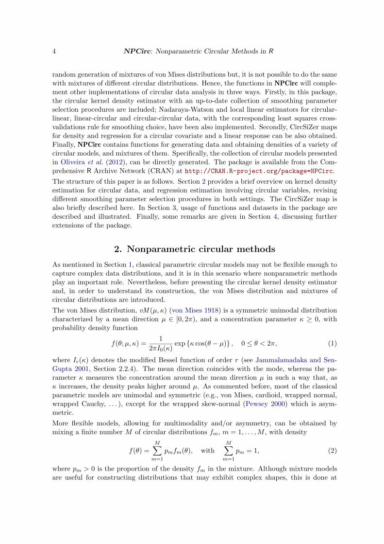
Before showing the circular kernel density estimator and the performance of the smoothingparameter selection methods, functions dcircmix and rcircmix will be described. Func-tion dcircmix computes the density function of a circular distribution (circular uniform, vonMises, cardioid, wrapped Cauchy, wrapped normal, wrapped skew-normal) or the density of amixture of these distributions. Function rcircmix allows for random generation from a circu-lar distribution or from a mixture of circular distributions. Both functions have an argumentcalled model which allows to specify a model among the ones considered in Oliveira et al.(2012). Throughout this work, random samples will be generated by fixing set.seed(2013),so the results can be reproduced by the user. For example, the density function of Model 18defined in Oliveira et al. (2012) on a grid of 500 points between 0 and 2π can be obtained by:

R> t <- circular(seq(0, 2 * pi, length = 500))

R> f18 <- dcircmix(x = t, model = 18)

and 100 random deviates from the same model can be obtained by:

R> data18 <- rcircmix(n = 100, model = 18)

http://www.puertos.es/

http://data.eol.ucar.edu/codiac/dss/id=85.034

http://data.eol.ucar.edu/codiac/dss/id=85.034


0

π

2

π

3π

2

+

●

●

●●

●

●

●

●

●

●

●

●

●

●

●

●

●

●

●

●

●

●●

●

●

●

●

●

●

●

●

●

● ●

●

●

●

●

●

●

●

●●

●

●

●

●

●

●

●●

●

●

●

●

●

●

●

●

●

●

●●

●

●

●●●

●

●

●

●

●

●

●

●●

●

●

●

●

●

●

●

●●

●

●

●●

●

●

●

●

●

●

●

●

●

●

0

π

2

π

3π

2

+

●

●●●

●

●

●

●

●

●

●

●

●

●

●

●

●

●

●

●

●

●●●

●

●

●

●●

●

●

●

●

●

●●

●

●

●

●

●

●

●

●

●

●

●●

●

●

●

●

●●

●●

●

●

●

●

●

●●

●

●

●

●

●

●●

●

●

●

●

●

●

●

●

●

●

●

●

●

●

●

●

●

●●

●●

●

●

●

●

●

●●

●

●

Figure 1: Left panel: density function (solid line) of the Model 18 from Oliveira et al. (2012)and a random sample of size n = 100 (dots on the circle). Right panel: density function (solidline) of the mixture model 0.5 · vM (0, 5) + 0.5 ·WSN (π, 1, 10) and a random sample of sizen = 100 (dots on the circle).

Note that argument x must be an object of class ‘circular’ (see Lund and Agostinelli 2013).

Both the model density curve and the random sample are plotted in Figure 1 (left panel).Functions from the circular package allow to plot the sample over a circle and the circulardensity as shown in the following lines

R> plot(data18, shrink = 1.2)

R> lines(t, f18, shrink = 1.2, lwd = 2)

which provide Figure 1 (left panel).

Apart from the predefined models from Oliveira et al. (2012), the density function or a randomsample from any mixture model can be obtained by using the same functions by specifying thedistributions that participate in the mixture through argument dist and the parameters ofeach distribution by means of argument param. For example, a mixture with equal proportionsof a von Mises vM (0, 5) and a wrapped skew-normal WSN (π, 1, 10) can be obtained with thecode:

R> fmix <- dcircmix(x = t, model = NULL, dist = c("vm", "wsn"),

+ param = list(p = c(0.5, 0.5), mu = c(0, pi), con = c(5, 1),

+ sk = c(0, 10)))

and random deviates from the same model can be obtained by:

R> datamix <- rcircmix(100, model = NULL, dist = c("vm","wsn"),

+ param = list(p = c(0.5, 0.5), mu = c(0, pi), con = c(5, 1),

+ sk = c(0, 10)))

The corresponding density function and random sample are shown in Figure 1 (right panel).

Function kern.den.circ

Function kern.den.circ computes the circular kernel density estimator with von Mises kernel(Equation 3), for the data sample specified by argument x (the object is coerced to class


‘circular’) and with a smoothing parameter included in argument bw. Unless the argumentt is provided, the estimator is computed over a grid of points specified by arguments from, toand len with default values, from = circular(0), to = circular(2 * pi) and len = 250.If no value of the smoothing parameter is provided by the user the circular kernel estimatoris computed with the value of the smoothing parameter selected by the plug-in rule. Theoutput of this function is an object of class ‘density.circular’ (see Lund and Agostinelli2013) whose underlying structure is a list containing the following components among others:data, the original dataset; x, the points where the density is estimated; y, the estimateddensity values; bw, the smoothing parameter used.

For a sample of 200 data from Model 7 from Oliveira et al. (2012), the circular kernel densityestimator can be obtained as follows:

R> data7 <- rcircmix(200, model = 7)

R> est7 <- kern.den.circ(x = data7, t = NULL, bw = 20, from = circular(0),

+ to = circular(2 * pi), len = 250)

R> est7

Call:

kern.den.circ(x = data7, t = NULL, bw = 20, from = circular(0),

to = circular(2 * pi), len = 250)

Data: data7 (200 obs.); Bandwidth 'bw' = 20

x y

n : 2.500e+02 Min. :0.01046

Min. :-3.129e+00 1st Qu.:0.04689

1st Qu.:-1.558e+00 Median :0.12702

Median : 0.000e+00 Mean :0.16015

Mean :-1.959e-14 3rd Qu.:0.26730

3rd Qu.: 1.558e+00 Max. :0.42007

Max. : 3.129e+00

Rho : 4.000e-03

R> names(est7)

[1] "data" "x" "y" "bw" "n" "kernel"

[7] "call" "data.name" "has.na"

The print method for ‘density.circular’ objects from package circular uses the output ofkern.den.circ to provide summaries of the estimation, as can be seen in the example.

The graphical display of the estimator is shown in Figure 2. Circular and linear representationsare displayed in left and right panels, respectively. The solid black line is the true underlyingdensity and the red curve is the circular kernel density estimator. These plots are obtainedby using the plot methods for ‘density.circular’ objects from package circular. A lines

method for ‘density.circular’ objects from package circular can be also used for addingother estimates to the plot.


N = 200 Bandwidth = 20 Unit = radians

Den

sity

circ

ular

0

π

2

π

3π

2

+

●

●

●

●●

●

●

●

●

●

●●

●

●

●

●

●

●

●

●

●

●

●●

●

●

●

●

●

●

●

●

●

●

●

●

●

●

●

●

●

●●

●

●

●

●

●

●

●

●

●

●

●●

●

●

●

●

●

●

●

●

●

●

●

●

●●

●●

●

●

●

●

●

●

●

●

●

●

●

●

●

●

●

●

●

●

●

●

●

●

●

●

●

●

●

●

●

●

●

●

●

●

●

●

●

●

●

●

●

●

●

●

●

●

●

●

●

●

●

●

●

●●

●

●

●

●

●

●

●

●

●

●

●

●

●

●

●

●

●

●

●

●

●

●

●

●

●●

●

●

●

●

●

●

●

●

●

●

●

●

●

●

●

●

●

●

●

●

●

●

●

●●

●

●

●

●

●

●

●

●

●

●

●

●

●

●

●

●

●

●

●

●

●

●

●

0 1 2 3 4 5 6

0.0

0.1

0.2

0.3

0.4

N = 200 Bandwidth = 20 Unit = radians

Den

sity

circ

ular

● ● ●●● ● ●● ●● ●●● ●● ●●●● ● ● ●● ● ● ●●● ● ●● ● ● ●● ● ●●● ●● ●●●● ●● ● ●● ● ●●●● ●●● ● ●● ●● ● ●● ● ●● ● ●● ●● ●● ● ●● ●● ●●● ● ●● ●● ●● ● ●●●● ●●● ●●●● ● ●●●● ●● ● ●● ● ●● ●●●● ● ●● ● ●●●● ● ●● ●● ●● ● ●● ●● ●● ●●● ●● ● ●● ●●●● ●●● ●● ●●● ●●● ●● ●● ●● ● ●●● ●●● ● ●● ● ●●● ●● ●● ●● ●●● ●● ●● ●●

Figure 2: Circular (left panel) and linear (right panel) representation of the circular kerneldensity estimator with ν = 20 (red line) of a sample of size 200 from Model 7 in Oliveira et al.(2012) and true density (black line).

The value of the parameter bw in function kern.den.circ can also be selected by some ofthe other rules defined in Section 2.1. The available procedures for choosing the smoothingparameter will be described below. The main argument in all the functions is the data fromwhich the smoothing parameter is to be computed, denoted by x. As before, the object iscoerced to class ‘circular’.

Function bw.boot implements the bootstrap procedure proposed by Marzio et al. (2011). Theminimum of the bootstrap MISE is obtained by using the optimize function from packagestats, which searches the minimum in the interval specified by arguments lower and upper

(default values are 0 and 50, respectively) and with accuracy specified by tol (default: tol

= 0.1). The integral is approximated by a sum of np = 500 terms.

R> bw.boot(x = data7)

[1] 14.68244

Cross-validation smoothing parameters for density estimation are computed by function bw.CV.The cross-validation rule to be used, LSCV or LCV, will be specified by argument method,taking LCV as default. When the LSCV smoothing parameter is computed, the integral termin Equation 8 is calculated using the Simpson’s rule (through an internal function) and so,the argument np will be used. As before, the minimum/maximum is searched with optimize

according to arguments lower, upper and tol.

R> bw.CV(x = data7, method = "LCV")

[1] 16.47961

R> bw.CV(x = data7, method = "LSCV")


[1] 15.91682

Function bw.pi implements the von Mises scale plug-in rule defined by Steps 1–3 in Sec-tion 2.1. Two options are available: fix the number of components in the mixture (denotedby M in Equation 2) by specifying argument M:

R> bw.pi(x = data7, M = 3)

[1] 26.4165

or select the number of components by AIC (default option):

R> bw.pi(x = data7, outM = TRUE)

[1] 25.86334 2.00000

Argument outM = TRUE indicates that the function also returns the number of componentsin the mixture. Again, the integral term is approximated by the Simpson’s rule and theminimum is searched by using the function optimize.

Finally, the selector proposed by Taylor (2008) for density estimation is computed by functionbw.rt. This selector is based on an estimation of the concentration parameter of a von Misesdistribution. The concentration parameter can be estimated by maximum likelihood (robust= FALSE):

R> bw.rt(x = data7, robust = FALSE)

[1] 0.1919247

or by the robustified procedure described before, by setting robust = TRUE. In this case, theargument alpha must be also specified:

R> bw.rt(x = data7, robust = TRUE, alpha = 0.5)

[1] 2.218956

Function circsizer.density

The CircSiZer map for density estimation is provided by circsizer.density. The mainarguments in this function are x, the angle data sample (object of class ‘circular’) andbws, a grid of positive smoothing parameters. Other arguments can be fixed: ngrid, integerindicating the number of equally spaced angles between 0 and 2π where the estimator is evalu-ated (default: ngrid = 250); alpha, the significance level for assessing increasing/decreasingpatterns (default: alpha = 0.05); B, the number of bootstrap samples to estimate the stan-dard deviation of f ′(θ; ν) (default: B = 500); log.scale, logical indicating if the values ofthe smoothing parameter are transformed to − log10 scale; and display, logical indicatingif the CircSiZer map is plotted. This function returns an object of class ‘circsizer’ whose


0

π

2

π

3π

2

+

Figure 3: Density for Model 14 from Oliveira et al. (2012) (left panel) and CircSiZer mapfor kernel density estimator (right panel) based on 100 simulated data (dots over the circle).Peaks and valleys are identified by clockwise blue-red and red-blue patterns, respectively.

underlying structure is a list containing the following components: data, the original dataset;ngrid, the number of equally spaced angles where the derivative of the circular kernel densityestimator is evaluated where the density is estimated, bw, a vector of smoothing parameters(given in − log10 scale if log.scale = TRUE); log.scale, logical indicating if − log10 scaleis used for constructing the CircSiZer map; CI, a list containing three matrices where eachrow corresponds to a value of the smoothing parameter and each column corresponds to anangle: a matrix with lower limits of the confidence intervals, a matrix with the upper limitsof the confidence intervals and a matrix with the effective sample size for each pair smoothingparameter-angle; and col, matrix containing the colors for plotting the CircSiZer map. Asfor the previous matrices, each entry contains the corresponding color for a pair of smoothingparameter-angle.

The CircSiZer map in Figure 3 is obtained with the following code lines:

R> data14 <- rcircmix(100, model = 14)

R> circsizer14 <- circsizer.density(data14, bws = seq(0, 100, by = 5),

+ ngrid = 250, alpha = 0.05, B = 500, log.scale = TRUE, display = TRUE)

R> names(circsizer14)

[1] "data" "ngrid" "bw" "log.scale" "CI" "col"

[7] "call" "data.name"

As noted before, in a CircSiZer map (see Figure 3), blue color indicates locations wherethe curve is significantly increasing; red color shows where it is significantly decreasing andpurple indicates where it is not significantly different from zero. Thus, for a given smoothingparameter, a significant peak can be identified when a region of significant positive gradient isfollowed by a region of significant negative gradient (i.e., blue-red pattern), and a significanttrough by the reverse (red-blue pattern), taking as sense of rotation the direction marked bythe arrow. Values of the smoothing parameter are indicated along the radius, transformedto − log10 scale for log.scale = TRUE (default option). Hence, in Figure 3, the multimodalstructure of the Model 14 from Oliveira et al. (2012) is clearly brought out by the CircSiZermap.


If display = FALSE, the CircSiZer map is not produced. However, the CircSiZer map can beplotted later by using the function circsizer.map whose main argument must be an objectof class circsizer. This function allows to edit the graph by specifying the arguments type,zero, clockwise, title, labels, label.pos, rad.pos and raw.data which allow to indicatethe zero of the plot, the sense of rotation, the title, the labels and their position, the positionof the radial lines and if the original data is plotted. For the above example, the code

R> circsizer.map(circsizer14, type = 4, zero = pi/2, clockwise = TRUE,

+ raw.data = TRUE)

provides the CircSiZer map but edited in another way (see Figure 3, right panel).

3.3. Illustration for regression estimation

For regression estimation with circular variables, NPCirc includes the following functions:kern.reg.circ.lin, kern.reg.circ.circ and kern.reg.lin.circ which allow to com-pute the local linear and Nadaraya-Watson estimators for circular-linear, circular-circularand linear-circular data, respectively. NPCirc also includes three functions for computing thecross-validation smoothing parameter in each case: bw.reg.circ.lin, bw.reg.circ.circ

and bw.reg.lin.circ. Finally, circsizer.regression allows to obtain the CircSiZer mapfor the regression setting when the covariate is circular and the response is linear.

Functions kern.reg.circ.lin, kern.reg.circ.circ and kern.reg.lin.circ

Functions kern.reg.circ.lin, kern.reg.circ.circ and kern.reg.lin.circ implementthe local linear estimator and the Nadaraya-Watson estimator for circular-linear data (circularcovariate and linear response), circular-circular data (circular covariate and circular response)and linear-circular data (linear covariate and circular response), respectively. The argumentsin these functions are: x, the vector of data for the independent variable; y, the vector ofdata for the dependent variable; t, the points where to evaluate the estimator; bw, the valueof the smoothing parameter to be used; method, a character string giving the estimator tobe used. This must be one of "LL" for local linear estimator or "NW" for Nadaraya-Watsonestimator. These functions return an object of class ‘regression.circular’ with a liststructure containing, among others, the following components: data the original dataset; x,the points where the regression function is estimated; y, the estimated values; and bw, thesmoothing parameter used.

For each function, the value of the smoothing parameter can be set manually or can beobtained by calling (default option) the functions bw.reg.circ.lin, bw.reg.circ.circ andbw.reg.lin.circ, respectively. These functions provide the least squares cross-validationsmoothing parameter for the Nadaraya-Watson and local linear estimators. For circular-linear data, the smoothing parameter is selected as the value that minimizes Equation 12.For circular-circular and linear-circular regression, minimization of Equations 13 or 14 providesmoothing parameters, the method in Equation 13 being the default option. The argumentsx, y and method of this function have the same meaning as before.

Functions kern.reg.circ.lin and bw.reg.circ.lin are illustrated with the wind.speed

dataset. The Nadaraya-Watson and local linear estimators for a regression model of windspeed over wind direction are shown in Figure 4 (left panel), in red and green lines respectively.Estimators are obtained with the code:


R> data("speed.wind2", package = "NPCirc")

R> dir <- speed.wind2$Direction

R> vel <- speed.wind2$Speed

R> nas <- which(is.na(vel))

R> dir <- circular(dir[-nas], units = "degrees")

R> vel <- vel[-nas]

R> bw.reg.circ.lin(dir, vel, method = "LL")

[1] 9.058419

R> bw.reg.circ.lin(dir, vel, method = "NW")

[1] 12.6612

R> estLL <- kern.reg.circ.lin(dir, vel, method = "LL"); estLL

Call:

kern.reg.circ.lin(x = dir, y = vel, method = "LL")

Data: dir (199 obs.); Bandwidth 'bw' = 9.058

x y

n : 2.500e+02 Min. :4.265

Min. :-1.793e+02 1st Qu.:6.927

1st Qu.:-8.928e+01 Median :7.557

Median : 0.000e+00 Mean :7.302

Mean :-6.647e-13 3rd Qu.:8.286

3rd Qu.: 8.928e+01 Max. :9.221

Max. : 1.793e+02

Rho : 4.000e-03

> estNW <- kern.reg.circ.lin(dir, vel, method = "NW"); estNW

Call:

kern.reg.circ.lin(x = dir, y = vel, method = "NW")

Data: dir (199 obs.); Bandwidth 'bw' = 12.66

x y

n : 2.500e+02 Min. :3.836

Min. :-1.793e+02 1st Qu.:7.062

1st Qu.:-8.928e+01 Median :7.712

Median : 0.000e+00 Mean :7.521

Mean :-6.647e-13 3rd Qu.:8.382

3rd Qu.: 8.928e+01 Max. :9.419

Max. : 1.793e+02

Rho : 4.000e-03


0 50 100 150 200 250 300 350

05

1015

direction

spee

d (m

/s)

●

●

●

●

●

●

●

●

●

●

●

●

●

●

●

●

●

●

●

●

●

●

●

●

●

●

●

●

●

●

●

●

●

●

●

●●

●

●

●

●

●

●

●

●

●

●

●

●●

●

●

●●

●

●

●

●

●

●

●

●

●●

●

●

● ●

●

●

●

●

●

●●

●

●

●

●

●

●

●

●

●

●

●

●●

●●

●

●

●

●

●

●

●

●

●

●

●

●

●●

●

●

●

●

●

●

●

●

●

●

●

●

●

●

●

●

●

●●

●

●

●

●

●

●

●

●

●

●

●

●

●

●

●

●

●●

●

●

●

●

●

●

●

●

●

●

●

●

●

●

●

●

●

●

●

●

●

●

●

●

●

●

●

●

●

● ●

●

●

●

●●

●

●

●

●

●

●

●

●

●

●

●

●

●

●

●

●

●

●

●

●

●

●

N

NE

E

SE

S

SW

W

NW

5 10 15 20

●

●

●●

●

●

●●

●

●

●

●

●

●

●

●

●

●

●

●

●

●

●●

●

●

●

●

●●

●

●

●

●

● ●

●

●

●

●

●

●

●●

●

●

●

● ●

●

●

●

●

●

●

●●

●

●

●

●

●

●

●

●

●

●

●

●

●

●

●

●

●

●●

●

●

●

●

● ●

●

●

●

●

●●

●

●

●

●

●

●

●

●

●

●

●

●

●

●

●

●

●

●

●

●

●

●

●

●

●

●●

●

●

●

●

●

●

●●

●

●

●

●

●

●

●

●

●

●

●

●

●

●

●

●

●

●

●

●

●

●

●

●

●●

●

●

●

●

●

●

●

●

●

●

●

●

●

●

●

●●

●

●

●

●

●

●

●

●

●

●

●●

●

●

●

●

●

●

●

●

●

●

●

●

●

●

●

●

●

●

●

●

●

Figure 4: Left and center: linear and circular representations of the Nadaraya-Watson estima-tor (red line) and local linear estimator (green line) with cross-validation smoothing parameterfor wind speed (m/s) with respect to wind direction. Right: CircSiZer map for circular-linearregression for wind speed (m/s) with respect to wind direction.

The objects (estNW and estLL), of class regression.circular, contain useful informationsuch as the original data, the fitted values or the smoothing parameter. This informationis used in the print method for ‘regression.circular’ objects to show summaries of thefitted model and in the plot and lines methods for ‘regression.circular’ objects, whichallow to plot the regression estimates. The following code lines produce the plots representedin Figure 4 (left and center):

R> plot(estNW, plot.type = "line", points.plot = TRUE, lwd = 2, line.col = 2,

+ xlab = "direction", ylab = "speed (m/s)")

R> lines(estLL, plot.type = "line", lwd = 2, line.col = 3)

R> res <- plot(estNW, plot.type = "circle", points.plot = TRUE,

+ labels = c("N", "NE", "E", "SE", "S", "SO", "O", "NO"),

+ label.pos = seq(0, 7 * pi/4, by = pi/4),

+ zero = pi/2, clockwise = TRUE, lwd = 2, line.col = 2, main = "")

R> lines(estLL, plot.type = "circle", plot.info = res, lwd = 2,

+ line.col = 3)

If plot.type = "line", a linear representation of the estimator is obtained. The periodicitycan be appreciated by joining the extremes of the lines. A circular representation can beproduced by setting plot.type = "circle".

Functions kern.reg.circ.circ and bw.reg.circ.circ are illustrated with the wind dataset.The circular-circular regression estimator is used to model the wind direction at noon, basedon the wind direction at 6 a.m. (see Marzio et al. 2012). The argument option indicatesthe cross-validation function to be used for selecting the smoothing parameter. If option =

1 (default option), then the criterion in Equation 13 is considered whereas if option = 2,Equation 14 is used:

R> data("wind", package = "NPCirc")

R> wind6 <- circular(wind$wind.dir[seq(7, 1752, by = 24)])

R> wind12 <- circular(wind$wind.dir[seq(13, 1752, by = 24)])


−3 −2 −1 0 1 2 3

−3

−2

−1

01

23

Wind direction at 6 a.m.

Win

d di

rect

ion

at n

oon

●●

●

●●

●

●

●

●

●

●

●

●

●

●

●

●

●

●

●

●

●

●●

●

●

●

●

●

●●

● ●

●

●

●●

●

●

●●

●

●

●

●

●

●

●

●

●

●●

●

●

●

●

●

●

●

●

●●

●

●

●

●

●

●

●

●

●

●

●

Figure 5: Representation on the torus (left panel) and linear representation (right panel) ofNadaraya-Watson (red line) and local linear (green line) estimators for wind directions atnoon with respect to wind directions at 6 a.m.

R> bw.reg.circ.circ(wind6, wind12, method = "LL", option = 1,

+ lower = 0, upper = 20)

[1] 2.834813

R> bw.reg.circ.circ(wind6, wind12, method = "NW", option = 1, lower = 0,

+ upper = 20)

[1] 5.482274

R> bw.reg.circ.circ(wind6, wind12, method = "LL", option = 2, lower = 0,

+ upper = 20)

[1] 2.252278

R> bw.reg.circ.circ(wind6, wind12, method = "NW", option = 2, lower = 0,

+ upper = 20)

[1] 6.080389

R> estNW <- kern.reg.circ.circ(wind6, wind12, t = NULL, bw = 6.1,

+ method = "NW")

R> estLL <- kern.reg.circ.circ(wind6, wind12, t = NULL, bw = 2.25,

+ method = "LL")

For circular-circular regression, the estimates can be plotted on a torus, by setting plot.type

= "circle" with the following code:

R> plot(estNW, plot.type = "circle", points.plot = TRUE, line.col = 2,

+ lwd = 2, points.col = 1, units = "degrees")

R> lines(estLL, plot.type = "circle", line.col = 3, lwd = 2)


0 20 40 60 80 100 120

5010

015

020

0

Distance (cms)

Dire

ctio

n (d

egre

es)

●●

●

●●●

●

●

●●

●

●

●

●

●

●

●

●

●●

●

●

●

●

●

●●

●

●

●

●

Figure 6: Representation on the cylinder (left panel) and linear representation (right panel)of the Nadaraya-Watson (red line) and local linear (green line) estimators for the periwinkle

data.

yielding the left plot in Figure 5. It should be noted that this is a 3D plot that can be rotated toexplore the characteristics of the fitted curve. To produce this graphic, packages misc3d (Fengand Tierney 2008) and rgl (Adler, Murdoch et al. 2014) are needed. Nevertheless, a linearrepresentation is also possible (plot.type = "line"). The linear plot of the observations at6 a.m. and noon, together with the Nadaraya-Watson and local-linear estimators are shownin Figure 5 (right) which have been obtained with the following code lines:

R> plot(estNW, plot.type = "line", points.plot = TRUE, line.col = 2, lwd = 2,

+ xlab = "Wind direction at 6 a.m.", ylab = "Wind direction at noon")

R> lines(estLL, plot.type = "line", line.col = 3, lwd = 2)

Finally, functions kern.reg.lin.circ and bw.reg.lin.circ are illustrated with the datasetperiwinkle. In this case, the linear-circular estimators are used to model the angles withregard to the distance moved:

R> data("periwinkles", package = "NPCirc")

R> dist <- periwinkles$distance

R> dir <- circular(periwinkles$direction, units = "degrees")

R> bw.reg.lin.circ(dist, dir, method = "NW", option = 1, lower = 0,

+ upper = 50)

[1] 21.24758

R> bw.reg.lin.circ(dist, dir, method = "NW", option = 2, lower = 0,

+ upper = 50)

[1] 21.50279

R> estNW <- kern.reg.lin.circ(dist, dir, t = NULL, bw = 21.25,

+ method = "NW")

R> estLL <- kern.reg.lin.circ(dist, dir, t = NULL, bw = 200, method = "LL")


For linear-circular regression, the estimates can be plotted on a cylinder (see Figure 6, leftpanel), by setting plot.type = "circle" with the following code:

R> plot(estNW, plot.type = "circle", points.plot = TRUE, line.col = 2,

+ lwd = 2, points.col = 2)

R> lines(estLL, plot.type = "circle", line.col = 3, lwd = 2)

A linear representation of the estimators is shown in Figure 6 (right panel).

Function circsizer.regression

The function circsizer.regression provides the CircSiZer map for regression, consideringa circular covariate and a linear response. The first arguments for this function are x, thedata for the circular covariate and y, the data for the dependent linear variable y. Theremaining arguments are the same as for function circsizer.density. If argument bws isnot specified (bws = NULL), a CircSiZer map for regression is, by default, computed for twovalues of the smoothing parameter. These two values are selected according to the value ofthe smoothing parameter provided by the corresponding least squares cross-validation ruleand the parameter adjust (by default adjust = 2). Thus, the CircSiZer map is obtained forthe values bw/adjust and bw * adjust.

Figure 4 (right panel) shows the CircSiZer map for exploring the relation between wind speedas a response and wind direction as a covariate, obtained with the code:

R> circsizer <- circsizer.regression(dir, speed, bws = seq(10, 60, by = 5),

+ display = FALSE)

R> circsizer.map(circsizer, type = 1, zero = pi/2, clockwise = TRUE)

In the CircSiZer map, it can be seen that wind speed increases when wind direction comesfrom NE and S-SW and winds from SE are not frequent at all, this fact being reflected bythe gray colored area.

As for the density setting, the output of the function circsizer.regression can be providedas the first argument of function circsizer.map in order to obtain a new CircSiZer map.

4. Conclusion and extensions

In this paper, the NPCirc package for performing nonparametric density and regression esti-mation with circular data in R is described, illustrating its performance with simulated andreal data examples. Thus, the package NPCirc contains functions for computing the nonpara-metric kernel circular density estimator and circular-linear, circular-circular and linear-circularregression estimators, which provide several useful tools for analyzing circular data withoutimposing parametric constraints. Moreover, for choosing a smoothing parameter, differentselectors, both for density and regression, have been revised and a graphical tool has beenproposed in order to avoid the smoothing parameter selection and explore the estimators atdifferent smoothing levels.

Circular data appear in a variety of disciplines and so, this package can be of interest tononparametric practitioners of different scientific fields.


In this current version, package NPCirc includes nonparametric methods based on the vonMises kernel. Different kernels or even, another kind of smoothers such as periodic splinescould be considered in order to extend the package.

Acknowledgments

The authors want to acknowledge two anonymous referees for their comments which helpedin improving both the paper and the package contents. The authors also acknowledgeProf. A. Pewsey for providing the dragonflies and cross beds data. Data from periglacial,collected within the Project POL2006–09071 from the Spanish Ministry of Education andScience have been provided by Prof. A. Perez-Alberti. Data stored in the wind dataset areprovided by NCAR/EOL under the sponsorship of the National Science Foundation.

This research has been supported by Project MTM2008–03010 from the Spanish Ministryof Science and Innovation, and by the IAP network StUDyS (Developing crucial Statisticalmethods for Understanding major complex Dynamic Systems in natural, biomedical and socialsciences), from Belgian Science Policy.

References

Abe T, Pewsey A (2011). “Symmetric Circular Models Through Duplication and CosinePerturbation.” Computational Statistics & Data Analysis, 55(12), 3271–3282.

Adler D, Murdoch D, et al. (2014). rgl: 3D Visualization Device System (OpenGL). R packageversion 0.94.1131, URL http://CRAN.R-project.org/package=rgl.

Bai ZD, Rao CR, Zhao LC (1988). “Kernel Estimators of Density Function of DirectionalData.” Journal of Multivariate Analysis, 27(1), 24–39.

Banerjee A, Dhillon IS, Ghosh J, Sra S (2005). “Clustering on the Unit Hypersphere Usingvon Mises-Fisher Distributions.” Journal of Machine Learning Research, 6(September),1345–1382.

Barragan S, Fernandez MA (2014). isocir: Isotonic Inference for Circular Data. R packageversion 1.1-3, URL http://www.CRAN.R-project.org/package=isocir.

Batschelet E (1981). Circular Statistics in Biology. Academic Press, New York.

Bowers JA, Morton ID, Mould GI (2000). “Directional Statistics of the Wind and Waves.”Applied Ocean Research, 22(1), 13–30.

Brunsdon C, Corcoran J (2005). “Using Circular Statistics to Analyse Time Patterns in CrimeIncidence.” Computers, Environment and Urban Systems, 30(3), 300–319.

Chaudhuri P, Marron JS (1999). “SiZer for Exploration of Structures in Curves.” Journal ofthe American Statistical Association, 94(447), 807–823.

Downs TD, Mardia KV (2002). “Circular Regression.” Biometrika, 89(3), 683–697.

http://CRAN.R-project.org/package=rgl

http://www.CRAN.R-project.org/package=isocir


Feng D, Tierney L (2008). “Computing and Displaying Isosurfaces in R.” Journal of StatisticalSoftware, 28(1), 1–24. URL http://www.jstatsoft.org/v28/i01/.

Fernandez-Duran JJ, Gregorio-Domınguez MM (2013). CircNNTSR: An R Package for theStatistical Analysis of Circular Data Using Nonnegative Trigonometric Sums (NNTS) Mod-els. R package version 2.1, URL http://www.CRAN.R-project.org/package=CircNNTSR.

Fisher NI (1993). Statistical Analysis of Circular Data. Cambridge University Press, Cam-bridge.

Fisher NI, Lee AJ (1992). “Regression Models for Angular Responses.” Biometrics, 48(3),665–677.

Hall P, Watson GP, Cabrera J (1987). “Kernel Density Estimation for Spherical Data.”Biometrika, 74(4), 751–762.

Hornik K, Grun B (2014). “movMF: An R Package for Fitting Mixtures of von Mises-FisherDistributions.” Journal of Statistical Software, 58(10), 1–31. URL http://www.jstatsoft.

org/v58/i10/.

Jammalamadaka SR, Lund UJ (2006). “The Effect of Wind Direction on Ozone Levels: ACase Study.” Environmental and Ecological Statistics, 13(3), 287–298.

Jammalamadaka SR, SenGupta A (2001). Topics in Circular Statistics. World Scientific,Singapore.

Jones MC, Pewsey A (2012). “Inverse Batschelet Distributions for Circular Data.” Biometrics,68(1), 183–193.

Kato S, Shimizu K, Shieh G (2008). “A Circular-Circular Regression Model.” Statistica Sinica,18(2), 633–645.

Klemela J (2000). “Estimation of Densities and Derivatives of Densities with DirectionalData.” Journal of Multivariate Analysis, 73(1), 18–40.

Lund U, Agostinelli C (2012). CircStats: Circular Statistics, from ‘Topics in Circular Statis-tics’ (2001). R package version 0.2-4, URL http://www.CRAN.R-project.org/package=

CircStats.

Lund U, Agostinelli C (2013). circular: Circular Statistics. R package version 0.4-7, URLhttp://www.CRAN.R-project.org/package=circular.

Mann KA, Gupta S, Race A, Miller MA, Cleary RJ (2003). “Application of Circular Statisticsin the Study of Crack Distribution Around Cemented Femoral Components.” Journal ofBiomechanics, 36(8), 1231–1234.

Mardia KV (1972). Statistics of Directional Data. Academic Press, New York.

Mardia KV, Jupp PE (2000). Directional Statistics. John Wiley & Sons, New York.

Marzio MD, Panzera A, Taylor CC (2009). “Local Polynomial Regression for Circular Pre-dictors.” Statistics & Probability Letters, 79(19), 2066–2075.

http://www.jstatsoft.org/v28/i01/

http://www.CRAN.R-project.org/package=CircNNTSR



http://www.CRAN.R-project.org/package=CircStats

http://www.CRAN.R-project.org/package=CircStats

http://www.CRAN.R-project.org/package=circular


Marzio MD, Panzera A, Taylor CC (2011). “Kernel Density Estimation on the Torus.” Journalof Statistical Planning & Inference, 141(6), 2156–2173.

Marzio MD, Panzera A, Taylor CC (2012). “Non-Parametric Regression for Circular Re-sponses.” Scandinavian Journal of Statistics, 40(2), 238–255.

Mooney JA, Helms PJ, Jollife IT (2003). “Fitting Mixtures of von Mises Distributions: ACase Study Involving Sudden Infant Death Syndrome.” Computational Statistics & DataAnalysis, 41(3–4), 505–513.

Oliveira M, Crujeiras RM, Rodrıguez-Casal A (2012). “A Plug-in Rule for Bandwidth Selectionin Circular Density Estimation.” Computational Statistics & Data Analysis, 56(12), 3898–3908.

Oliveira M, Crujeiras RM, Rodrıguez-Casal A (2013). “Nonparametric Circular Methods forExploring Environmental Data.” Environmental and Ecological Statistics, 20(1), 1–17.

Oliveira M, Crujeiras RM, Rodrıguez-Casal A (2014a). “CircSiZer: An Exploratory Tool forCircular Data.” Environmental and Ecological Statistics, 21(1), 143–159.

Oliveira M, Crujeiras RM, Rodrıguez-Casal A (2014b). NPCirc: Nonparametric Circu-lar Methods. R package version 2.0.1, URL http://www.CRAN.R-project.org/package=

NPCirc.

Parzen E (1962). “On Estimation of a Probability Density Function and Mode.” The Annalsof Mathematical Statistics, 33(3), 1065–1076.

Pewsey A (2000). “The Wrapped Skew-Normal Distribution on the Circle.” Communicationsin Statistics – Theory and Methods, 29(11), 2459–2472.

Presnell B, Morrison SP, Littel RC (1998). “Projected Multivariate Linear Models for Direc-tional Data.” Journal of the American Statistical Association, 93(443), 1068–1077.

R Core Team (2014). R: A Language and Environment for Statistical Computing. R Founda-tion for Statistical Computing, Vienna, Austria. URL http://www.R-project.org/.

Qin X, Zhang JS, Yan XD (2011a). “Local Linear Least Squares Kernel Regression for Linearand Circular Predictors.” Communications in Statistics – Theory and Methods, 40(21),3812–3823.

Qin X, Zhang JS, Yan XD (2011b). “A Nonparametric Circular-Linear Multivariate Regres-sion Model with a Rule-of-Thumb Bandwidth Selector.” Computers & Mathematics withApplications, 62(8), 3048–3055.

Rosenblatt M (1956). “Remarks on Some Nonparametric Estimate of a Density Function.”The Annals of Mathematical Statistics, 27(3), 832–837.

SenGupta A, Ugwuowo FI (2006). “Asymmetric Circular-Linear Multivariate Regression Mod-els with Applications to Environmental Data.” Environmental and Ecological Statistics,13(3), 299–309.

http://www.CRAN.R-project.org/package=NPCirc

http://www.CRAN.R-project.org/package=NPCirc

http://www.R-project.org/


SenGupta S, Rao JS (1966). “Statistical Analysis of Cross-Bedding Azimuths from the KamthiFormation around Bheemaram, Pranhita: Godavari Valley.” Sankhya: The Indian Journalof Statistics B, 28(1/2), 165–174.

Taylor CC (2008). “Automatic Bandwidth Selection for Circular Density Estimation.” Com-putational Statistics & Data Analysis, 52(7), 3493–3500.

von Mises R (1918). “Uber die “Ganzzahligkeit” der Atomgewichte und verwandte Fragen.”Physikalische Zeitschrift, 19, 490–500.

Affiliation:

Marıa Oliveira, Rosa M. Crujeiras, Alberto Rodrıguez-CasalDepartment of Statistics and Operations ResearchFaculty of MathematicsUniversity of Santiago de CompostelaSpainE-mail: [email protected], [email protected],

[email protected]

Journal of Statistical Software http://www.jstatsoft.org/

published by the American Statistical Association http://www.amstat.org/

Volume 61, Issue 9 Submitted: 2013-03-29October 2014 Accepted: 2014-06-03

mailto:[email protected]



http://www.jstatsoft.org/

http://www.amstat.org/

NPCirc: An R Package for Nonparametric Circular Methods

Documents

Transcript of NPCirc: An R Package for Nonparametric Circular Methods