Detached eddy simulation of shock unsteadiness in an over-expanded planarnozzle

E. Martellia,∗, P.P. Ciottolib, M. Bernardinib, F. Nasutib, M. Valoranib

aSecond University of Naples, 81031 Aversa, ItalybUniverity of Rome ”La Sapienza”, 00184 Rome, Italy

Abstract

This work investigates the self-excited shock wave oscillations in a three-dimensional planar over-expanded nozzleturbulent flow by means of Detached Eddy Simulations. Time resolved wall pressure measurements are used asprimary diagnostics. The statistical analysis reveals that the shock unsteadiness has common features in terms ofthe root mean square of the pressure fluctuations with other classical shock wave/boundary layer interactions, likecompression ramps and incident shocks on a flat plate. The Fourier transform and the continuous wavelet transformare used to conduct the spectral analysis. The results of the former indicate that the pressure in the shock regionis characterized by a broad low-frequency content, without any resonant tone. The wavelet analysis, which is wellsuited to study non stationary process, reveals that the pressure signal is characterized by an amplitude and a frequencymodulation in time.

1. Introduction

During the sea-level start-up of a liquid rocket engine the nozzle is highly overexpanded and an internal flowseparation takes place, characterized by a shock wave boundary layer interaction (SWBLI), which causes the sheddingof vortical structures and unsteadiness in the shock wave position. In the nozzle design community, flow separationis considered dangerous, since it produces dynamic side-loads that reduce the safe life of the engine and can leadto a failure of the nozzle structure. The need to improve nozzle performance under overexpanded conditions and tomitigate the side loads fostered several experimental [1, 2, 3] and numerical investigations [4, 5, 6]. All these studiesrevealed two distinct separation processes: the free shock separation (FSS), in which the boundary layer separates fromthe nozzle wall and never reattaches, and the restricted shock separation (RSS), characterized by a closed recirculationbubble and the reattachment of the shear layer to the wall.

According to Schmucker [7], the main cause of side-loads appearance is an asymmetry of the separation location,which produces a tilted separation line, a momentum imbalance and consequently a lateral force. Nave and Coffey [1]observed that, in optimized nozzles, the maximum value of the side loads takes place during the transition from FSSto RSS condition. A literature survey reporting the various studies on the side loads generation and separation shockconfigurations can be found in Hadjadj and Onofri [8] and in Reijasse et al. [9]. But, in spite of all of these studies, afundamental knowledge of supersonic flow physics in the presence of a shock separation interaction is still needed.

One of the several tasks for future investigations recommended by Hadjadj and Onofri [8] is related to the lowfrequency oscillations of a shock interacting with a turbulent flow separation. This phenomenon, consisting in fluctu-ating pressure loads and pulsating separated flows, should be carefully considered by rocket nozzle designers. A lotof experimental work has been carried out to understand the unsteadiness of shocks in internal flows. Bogar et al. [10]investigated the unsteady flow characteristics of a supercritical transonic diffuser as a function of shock Mach numberand diffuser length. They observed that in the case of attached flow (or very mild separation), the characteristic fre-quencies have an acoustic nature, and scale with the distance of the shock from the diffuser exit. While, in the case of

∗Corresponding authorEmail address: emanuele.martelli@unina2.it (E. Martelli)

1

arX

iv:1

606.

0511

4v1

[ph

ysic

s.fl

u-dy

n] 1

6 Ju

n 20

16

separated flows, the characteristic frequencies scale with the length of the inviscid core flow. Zaman et al[11] carriedout experiments in a supersonic planar diffuser, and documented a transonic tone with weak harmonics. The presenceof harmonics led to the theory that the observed frequency was caused by an acoustic feed-back mechanism.

In addition, they found that the instability has the higher sound pressure level if the boundary layer before theshock is laminar, while if the boundary layer is tripped, in some of the tests the tone was suppressed. Both Bogar andZaman underlined that the mechanism for the shock instability is unclear, although they indicate some dependency ofthe shock dynamics on the downstream separated region. Also Handa et al. [12], in their experimental investigationof a transonic diffuser, underlined two different mechanisms for the shock oscillation. In the first mechanism, pressuredisturbances, generated in the downstream turbulent separated region, force the shock to oscillate, resulting in a broadshape of the power spectral density. In addition, the intensity of this movement is mainly governed by the Mach num-ber in front of the shock. The second mechanism foresees the reflection of a disturbance at the diffuser exit (acousticfeedback), resulting in a narrow-shaped power spectral density. More recently, Johnson and Papamoschou [13] havestudied the unsteady shock behavior in an over-expanded planar nozzle. Their results indicate a low frequency piston-like shock motion without any resonant tones. Correlations of Pitot pressure with wall pressure indicated a strongcoherence of the shear layer instability with the shock motion. All these different experimental investigations suggesta correlation between the shock movement and the acoustic or fluid dynamic characteristics downstream of the flowseparation.

As far as Large/Detached Eddy Simulations (LES/DES) of this kind of flows are concerned, very few studies canbe found in literature. Deck [14] carried out a Delayed Detached Eddy Simulation (DDES) of the end-effect regime inan axi-symmetric over-expanded rocket nozzle flow. While the experimentally measured main properties of the flowmotion were rather well reproduced, the computed main frequency resulted to be higher than in the experiment. Olsonand Lele [15] performed large eddy simulations of the experiments of Papamoschou, finding a satisfactory agreementbetween the experimental data and the computed frequency of the shock displacement. The origin of the unsteadinesswas attributed to the confinement of exit area by the separated flow.

In the present work, Delayed Detached Eddy Simulations (DDES) reproducing the flowfield of the nozzle geom-etry of Bogar et al. [10] are carried out to completely characterize the shock unsteadiness at different nozzle pressureratios. Resorting to this computational strategy, any perturbation coming from the upstream boundary layer is notresolved. Therefore the separation shock can only be perturbed by the turbulent recirculating region. In a recentreview of Clemens et al. [16] on the low frequency unsteadiness of the shock wave/turbulent boundary layer interac-tion, it is argued that both upstream and downstream perturbations are at work in the interaction, whether there is aseparation bubble or not. However, the influence of the upstream turbulent boundary layer decreases when the sizeof the separation bubble increases. In flow separated nozzle, the recirculation bubble is longer than in other classicalconfiguration like the compression ramp. Therefore it seems reasonable to attribute the most important influence onthe shock movement to the downstream region. In such a case, the DDES technique can be considered adequate.Following the literature [17], the unsteady behavior of shock flow separation interaction is characterized by analyzingthe time series of the wall pressure signals. In particular, the stream-wise distributions of the root mean square as wellas the probability density functions (pdf) of the pressure signals are discussed. Then the intermittency of the signalsis computed, and from its distribution the length scale of the shock motion is quantified, this quantity being directlylinked to the level of the side-loads.

The shock flow separation interaction is characterized by the presence of several dominating components in thepressure fluctuations, connected to the development of vortical structures and to the shock movement itself. Fourieranalysis is used in order to evaluate the main frequencies along the nozzle, from the shock location to the turbulentrecirculating zone. In addition to the global spectral characterization, it is of great interest to understand if the domi-nating components are simultaneously or alternatively present, and to characterize the time variation of their frequencyand amplitude. The wavelet transform is an analysis tool well suited to the study of multi-scale, non-stationary pro-cesses occurring over finite temporal domains. In particular, it allows to detect the localized variations of power withina time series. In fact, by decomposing a time series into time-frequency space, it is possible to determine both thedominant modes of variability, as well as their time evolution. Therefore, the continuous complex wavelet transformis directly applied in order to identify the time modulation of frequency and amplitude of turbulent structures [18].This characterization contributes to the basic understanding of the shock wave/turbulent boundary layer interactionphysics in internal flows. A better knowledge of this phenomenon can help in predicting and possibly control the levelof side loads, thus allowing the design of larger area ratio nozzle, improving the nozzle performance and reducing the

2

costs of the access to space.The paper is organized as follows. In section 2 the numerical method is introduced and the use of DDES is

discussed in the frame of over-expanded nozzles. Section 3 presents the experimental test cases and the numericalsetup. Section 4.1 presents the mean properties of the fields and of the wall pressure distributions, together with thestatistical description of the shock separation iteration. Fourier and the wavelet spectral analysis are discussed inSection 4.2 and Section 4.3 respectively. Finally, in the conclusion section the major findings of this investigation arereported.

2. Computational setup

To better understand the unsteadiness of SWBLI in supersonic nozzles and the role played in the generation ofside loads, large eddy simulations should be ideally carried out to capture the larger structures of the turbulent flow.Unfortunately, the computational cost of a pure (wall-resolved) LES is still very high for high-Reynolds number wall-bounded flows. To overcome this limitation, hybrid RANS/LES modeling approaches have been proposed to simulatemassively separated flows, such as the well-known DES [19]. A general feature of this approach is that the wholeor at least a major part of the attached boundary layer is treated resorting to RANS, while LES is applied only inthe separated flow regions. In the following a brief description of the numerical solver used is given, then the maincharacteristics of DDES are outlined.

2.1. Physical model

We solve the three-dimensional Navier-Stokes equations for a compressible, viscous, heat-conducting gas

∂ρ

∂t+∂(ρ u j)∂x j

= 0,

∂(ρ ui)∂t

+∂(ρ uiu j)∂x j

+∂p∂xi−∂τi j

∂x j= 0,

∂(ρ E)∂t

+∂(ρ Eu j + pu j)

∂x j−∂(τi jui − q j)

∂x j= 0,

(1)

where ρ is the density, ui is the velocity component in the i-th coordinate direction (i = 1, 2, 3), E is the total energyper unit mass, p is the thermodynamic pressure. The total stress tensor τi j is the sum of the viscous and the Reynoldsstress tensor,

τi j = 2 ρ (ν + νt) S ∗i j S ∗i j = S i j −13

S kk δi j, (2)

where the Boussinesq hypothesis is applied through the introduction of the eddy viscosity νt, and where S i j =(ui, j + u j,i

)/2 is the strain-rate tensor, ν the molecular viscosity, depending on temperature T through Sutherland’s

law. Similarly, the total heat flux q j is the sum of a molecular and a turbulent contribution

q j = −ρ cp

(ν

Pr+νt

Prt

)∂T∂x j

, (3)

Pr, Prt being the molecular and turbulent Prandtl numbers, assumed to be 0.72 and 0.9, respectively. Hybrid RANS/LEScapabilities are provided through the implementation of the delayed detached-eddy simulation (DDES) approachbased on the Spalart-Allmaras (SA) model [20], which involves a transport equation for a pseudo eddy viscosity ν

∂(ρν)∂t

+∂(ρ ν u j)∂x j

= cb1S ρν +1σ

∂

∂x j

[(ρν + ρν)

∂ν

∂x j

]+ cb2 ρ

(∂ν

∂x j

)2 − cw1 fwρ(ν

d

)2, (4)

where d is the model length scale, fw is a near-wall damping function, S a modified vorticity magnitude, andσ, cb1, cb2, cw1 model constants. The eddy viscosity in Eq. 2 is related to ν through νt = ν fv1, where fv1 is a cor-rection function designed to guarantee the correct boundary-layer behavior in the near-wall region. In DDES the

3

destruction term in Eq. 4 is designed so that the model reduces to pure RANS in attached boundary layers and to aLES sub-grid scale one in the detached flow regions. This is accomplished by defining the length scale d as

d = dw − fd max (0, dw −CDES ∆) , (5)

where dw is the distance from the closest wall, ∆ is the subgrid length-scale, controlling the wavelengths resolved inLES mode. The function fd, designed to be 0 in boundary layers and 1 in LES regions, reads as

fd = 1 − tanh[(8rd)3

], rd =

ν

k2 d2w

√Ui, jUi, j

, (6)

where Ui, j is the velocity gradient and k the von Karman constant. The introduction of fd distinguishes DDES from theoriginal DES approach [21] (usually denoted as DES97), ensuring that boundary layers are treated in RANS mode alsoin the presence of “ambiguous” grids in the sense defined by Spalart et al. [20], for which the wall-parallel spacingsdo not exceed the boundary layer thickness. The DDES strategy prevents the phenomenon of model stress depletion,consisting in the excessive reduction of the eddy viscosity in the region of switch (grey area) between RANS and LES,which in turn leads to grid-induced separation. Unlike in the original DDES formulation, the sub-grid length scale inthis work is not defined as the largest spacing in all coordinate directions ∆max = max(∆x,∆y,∆z), but it depends onthe flow itself, through fd as follows

∆ =12

[(1 +

fd − fd0

| fd − fd0|

)∆max +

(1 −

fd − fd0

| fd − fd0|

)∆vol

], (7)

where fd0 = 0.8, ∆vol = (∆x · ∆y · ∆z)1/3. The improvement over the classical ∆max definition is shown in Deck [22],where the problem of the delay in the formation of flow instabilities encountered in early applications of DES/DDESis solved.

2.2. Numerical method

Numerical simulations are carried out by means of a in-house, fully validated compressible flow solver, thatexploits a centered second-order finite volume approach and takes advantage of an energy consistent formulation(away from shocks). Cell-face values of the flow variables are obtained from the cell-centered values through suitablereconstructions. In smooth flow regions, the reconstruction is carried out in such a way that the overall kineticenergy of the fluid is preserved, in the limit of inviscid, incompressible flow [23]. This property is particularlybeneficial for flow regions treated in LES mode, where the grid is sufficiently fine to support the development of LEScontent, and where the only relevant dissipation (in addition to the molecular one) should be that provided by theturbulence model. The discretization scheme is made to switch to third-order weighted essentially-non-oscillatory(WENO) near discontinuities, as controlled by a modified Ducros sensor [24]. The gradients normal to the cellfaces needed for the viscous fluxes, are evaluated through second-order central-difference approximations, obtainingcompact stencils and avoiding numerical odd-even decoupling phenomena. Time advancement of the semi-discretizedsystem of ODEs resulting from the spatial discretization is carried out by means of a low-storage third-order Runge-Kutta algorithm [25]. The code is written in Fortran 90, it uses domain decomposition and it fully exploits the MessagePassing Interface (MPI) paradigm for the parallelism.

3. Test case description

The experimental diffuser model numerically reproduced in this work is a convergent-divergent channel with a flatbottom and a contoured top wall, as shown in figure 1. The analytical expression of the contoured wall can be foundin Bogar et al. [10] The channel height at the throat is 44 mm, the exit-to-throat area ratio is 1.52, the throat cross-sectional aspect ratio is 4.0, and the divergent length to throat height ratio is 7.2. For x/Ht greater than 7.2 the nozzleis characterized by a constant area section. In the experimental case dry air is supplied to the model from a plenumchamber immediately upstream. The flow from the model is vented to the atmosphere, providing a constant-pressuredownstream boundary condition.

4

Figure 1: Two-dimensional schematic of the computational domain with boundary conditions

Figure 2: Experimental mean top wall pressure distribution [10], compared with a 2D RANS simulation for NPR = 1.39

A two-dimensional schematic of the computational domain adopted in the simulations is presented in figure 1.According to Bogar et al. [10] an arbitrarily selected location within the constant area section upstream of the throat(xi/Ht = −4.04) has been chosen as a nominal inlet section. The nominal exit section is at xe/Ht = 12.63. In theinlet station a subsonic flow is prescribed by imposing the Mach number M = 0.46, the static pressure and the flowdirection. The top and bottom surfaces are treated as adiabatic no-slip walls. In the spanwise direction the extent ofthe domain is Lz/Ht = 4, and periodic boundary conditions are imposed. At the exit section a characteristics basedboundary condition prescribing the back pressure is assigned. In order to avoid any acoustic coupling a sponge isimposed from the station at x/Ht = 9. As stated in the introduction, in fact, the effect of the acoustic feed back isless important when a large recirculating bubble is present. A logically Cartesian structured mesh is generated usingthe conformal mapping algorithm of Driscoll and Vavasis[26] and the open-source tool gridgen-c. The computationalmesh consists in Nx · Ny · Nz = 512 · 192 · 256 cells for a total number of Nxyz ≈ 25 · 106 cells.

The present internal flowfield is characterized by the nozzle pressure ratio NPR = p0/pa, where p0 and pa denotethe chamber and ambient pressure respectively. In this work three different values are simulated: 1.39, 1.46 and 1.54.The NPR’s values are changed by decreasing the back pressure at the exit section, so that the nozzle Reynolds number

5

(a) (b)

Figure 3: Time-averaged and span-wise averaged field of: a) ||∇ρ|| and b) density (isolines) with the region with negative velocities (coloured) inthe transonic nozzle at different NPR’s.

based on the chamber values and the throat height remains constant:

Re =

√γ

µ

pcHt√

RairT0= 1.5 · 106,

where γ is the constant specific heat ratio, µ is the molecular viscosity evaluated at the chamber temperature T0 andRair is the air gas constant. A preliminary 2D RANS simulation was performed in order to verify that the meshresolution in the longitudinal and wall normal direction is sufficient to capture the position of separation line. Thecomparison of the computed top wall pressure distribution with the experiment [10] for NPR = 1.39 is reported infigure 2, and it shows that both the position of the separation point and the pressure behavior in the separated zone arewell reproduced.

4. Results and discussion

4.1. Time-averaged and instantaneous flowfield

The time and spanwise averaged numerical Schlieren like visualizations (||∇ρ||) of the three NPR’s are presentedin Figure 3. The flowfield is characterized by a lambda shock, a recirculation zone and a shear layer. As the NPRincreases, the separation shock moves downstream, while the height of the Mach stem decreases. The evolution of therecirculation bubble with the NPR is shown in figure 3b where an enlargement of the back flow region (indicated bythe coloured flood region) with the downstream movement of the separation shock can be observed.

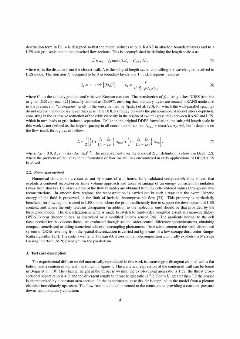
The top wall pressure distributions in the streamwise direction are presented in figure 4a for the different NPR’s.It can be noted the steep increase of the wall pressure due to the lambda foot of the separation shock, then the flatbehavior in the separation bubble and finally a mild increase to the back pressure value in the final part of the diffuser.The isentropic Mach number distribution in the streamwise direction is reported in Figure 4b. This value is computed

from the isentropic relation between the chamber pressure and wall pressure p0/pw =(1 +

γ−12 M2

i

) γγ−1 and it is used to

characterize the shock intensity in nozzle separated flows and to reduce the data from different experiments [27]. Theisentropic Mach numbers characterizing the shock intensities for the test cases with NPR = 1.39, 1.46, and 1.54 areMi = 1.34, 1.41, and 1.52. The lower value is close to the experimental value of the work of Bogar et al[10], whilethe other two are higher. It must be noted that Bogar, in order to characterize the shock intensity, employed the localMach number at the edge of the top wall boundary layer immediately upstream of the shock, instead of the isentropicMach number. Nonetheless, the two numerical values do not differ significantly.

6

(a) (b)

Figure 4: Left: streamwise distributions of time and spanwise averaged wall pressure. Right: streamwise distributions of the wall isentropic Machnumber, indicating the shock strength

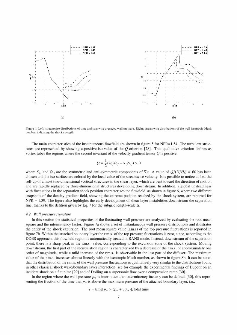
The main characteristics of the instantaneous flowfield are shown in figure 5 for NPR=1.54. The turbulent struc-tures are represented by showing a positive iso-value of the Q-criterion [28]. This qualitative criterion defines asvortex tubes the regions where the second invariant of the velocity gradient tensor Q is positive:

Q =12

(Ωi jΩi j − S i jS i j) > 0

where S i j and Ωi j are the symmetric and anti-symmetric components of ∇u. A value of Q/(U/Ht) = 60 has beenchosen and the iso-surface are colored by the local value of the streamwise velocity. Is is possible to notice at first theroll-up of almost two-dimensional vortical structures in the shear layer, which are bent toward the direction of motionand are rapidly replaced by three-dimensional structures developing downstream. In addition, a global unsteadinesswith fluctuations in the separation shock position characterizes the flowfield, as shown in figure 6, where two differentsnapshots of the density gradient field, showing the extreme position reached by the shock system, are reported forNPR = 1.39. The figure also highlights the early development of shear layer instabilities downstream the separationline, thanks to the defition given by Eq. 7 for the subgrid length-scale ∆.

4.2. Wall pressure signatureIn this section the statistical properties of the fluctuating wall pressure are analyzed by evaluating the root mean

square and the intermittency factor. Figure 7a shows a set of instantaneous wall pressure distributions and illustratesthe entity of the shock excursion. The root mean square value (r.m.s) of the top pressure fluctuations is reported infigure 7b. Within the attached boundary layer the r.m.s. of the top pressure fluctuations is zero, since, according to theDDES approach, this flowfield region is automatically treated in RANS mode. Instead, downstream of the separationpoint, there is a sharp peak in the r.m.s. value, corresponding to the excursion zone of the shock system. Movingdownstream, the first part of the recirculation region is characterized by a decrease of the r.m.s. of approximately oneorder of magnitude, while a mild increase of the r.m.s. is observable in the last part of the diffuser. The maximumvalue of the r.m.s. increases almost linearly with the isentropic Mach number, as shown in figure 8b. It can be notedthat the distribution of the r.m.s. of the wall pressure fluctuations is qualitatively very similar to the distributions foundin other classical shock wave/boundary layer interaction; see for example the experimental findings of Dupont on anincident shock on a flat plate [29] and of Dolling on a supersonic flow over a compression ramp [30].

In the region where the wall pressure pw is intermittent, an intermittency factor γ can be defined [30], this repre-senting the fraction of the time that pw is above the maximum pressure of the attached boundary layer, i.e.,

γ = time[pw > (pw + 3σw)]/total time

7

Figure 5: Iso-surface of the Q-criterion (Q/(U/Ht) = 60), colored by the local value of the streamwise velocity, for NPR = 1.54. The shock isvisualized by an iso-surface of ∇ · u; the slice in the Z-plane shows the field of ||∇ρ||.

For the undisturbed boundary layer, the experimental value of γ is equal to 0.0015 (close to the theoretical Gaussianvalue of 0.0013). In the RANS simulated attached boundary layer the value of γ would be zero. An intermittencyequal to 0.5 corresponds to case of having the same probability for the shock to be located on the left and on theright of the probe, and coincide with the maximum value in the r.m.s. distribution. The streamwise evolutions ofthe intermittency for the various NPR’s are shown in figure 8a. All the distributions of the intermittency versus x/Ht

have the same shape, with the value of 0.5 occurring at the same abscissa of the maximum r.m.s. value. This shapeis similar to the one produced by the shock in a supersonic ramp flow (Dolling et al. [30]). The distribution of γ canbe used to evaluate the shock excursion length. In fact, at any instant, the furthest upstream position of the separationshock is where the incoming boundary layer is firstly disturbed. Thus the distance over which γ increases from 0.0015(from zero in the present simulations) to 1 is the absolute length scale Ls of the shock motion. Figure 8b shows thenondimensional shock excursion length scale Ls/Ht as a function of the isentropic Mach number Mi. It can be seenthat the trend is almost linear, with an increase of 11% in the value of Ls/Ht when rising the isentropic Mach numberfrom 1.34 to 1.52.

The pre-multiplied spectra f E( f ) of the pressure signal at the top wall are shown in figure 9 for the differentNPR’s as a function of the dimensional frequency f and the streamwise coordinate x/Ht. The power spectral densitieshave been computed using the Welch method, subdividing the overall pressure record into K segments with 50%overlapping, which are individually Fourier-transformed. The frequency spectra are then obtained by averaging theperiodograms of the various segments, which allows to minimize the variance of the PSD estimator, and by applyinga Konno-Omachi smoothing filter [31], which ensures a constant bandwidth on a logarithmic scale. The number ofsegments is K = 10 for the three cases here investigated. The spectral maps are characterized by two different zones,qualitatively similar for the various NPR’s. The first region is associated with the dynamics of the shock system andis identified by a peak whose characteristic frequency is of the order O(200)Hz, located in the proximity of the shockfoot. We point out that, while previous investigations based on URANS identified the shock motion as tonal [32],the low-frequency activity predicted by our DDES is rather broadband, the energy content encompassing a wholedecade of frequencies. This behavior is in agreement with recent experiments and LES carried out for canonicalsupersonic boundary layer interactions [29, 33, 34, 35]. The second extended region in the spectral densities is thesignature of the turbulent activity in the separation bubble, whose dynamics is well captured by the LES branch of

8

(a)

Figure 6: Numerical Schlieren at two different time instants for NPR = 1.39.

(a) (b)

Figure 7: a): Streamwise distributions of instantaneous spanwise averaged wall pressure; b): streamwise distributions of time and spanwiseaveraged wall pressure and the pressure root mean square.

9

(a) (b)

Figure 8: a): streamwise distribution of the intermittency factor. b): streamwise length of the shock motion Ls and maximum value of the pressurer.m.s. as a function of the wall isentropic Mach number.

(a) NPR = 1.54

(b) NPR = 1.46

(c) NPR = 1.39

Figure 9: Pre-multiplied spectra ( f E( f )) of the top wall pressure at various NPR’s. The horizontal dashed line denotes the peak frequency of theshock motion.

10

Figure 10: Morlet Wavelet base: a) real part (solid line) and imaginary part (dashed line) in the time domain; b) the corresponding wavelet in thefrequency domain.

the simulations. The peak of the frequency spectra in this zone is centered around f ≈ 2500Hz and its streamwiselocation approximately correspond to the reattachment point. This qualitative scenario is shared by the various NPR’s.The main effect of increasing the NPR is to shift downstream the location of the low-frequency peak and to (slightly)decrease the characteristic frequency of the oscillations (see section 4.3.2 for a comparison with experiments).

4.3. Wavelet spectral analysis

4.3.1. Morlet wavelet transformThe continuous wavelet transform is applied to the unsteady wall pressure signals in order to decompose them in

the time-frequency space. An extended review of the application of wavelets to study turbulence phenomena can befound in Farge [18], while only the key theoretical aspects are here reported. The continuous wavelet transform of adiscrete time sequence pn, with equal spacing δt and n = 0...N − 1, is defined as the convolution of pn with a scaledand translated version of the mother wavelet ψ0:

Wn(s) =

N−1∑n′=0

pn · ψ∗

[(n′ − n)δt

s

](8)

where ∗ denotes the complex conjugate. By varying the wavelet scale s and translating along the time index n, onecan construct a picture showing both the amplitude of any features versus the scale and how this amplitude varies withtime. In this study, the Morlet wavelet has been chosen since higher resolution in frequency can be achieved whencompared with other mother functions. It consists of a plane wave modulated by a Gaussian:

ψ0(η) = π−1/4eiω0ηe−η2/2 (9)

where η is a nondimensional time parameter and ω0 is the nondimensional frequency, here taken equal to 6 to satisfythe admissibility condition [36]. This wavelet is shown in figure 10 both in the time and frequency domains. From thedefinition of the wavelet coefficient one can directly define the wavelet power spectrum (WPS) as |Wn(s)|2. The totalenergy is conserved under the wavelet transform and the equivalent of the Parseval’s theorem for wavelet analysis is

σ2 =δ jδtCδN

N−1∑n=0

J∑j=0

|Wn(s)|2

s j(10)

where σ2 is the variance, δ j is the scale spacing and Cδ is a factor coming from the reconstruction of a δ functionfrom its wavelet transform. For more details the interested reader could see the work of Torrence and Compo [36].The energy density is then determined as:

E(s, t) =|Wn(s)|2

s j(11)

11

Once a wavelet function has been chosen, it is necessary to determine a set of scales s to use in the transform. Inthe case of non orthogonal wavelet analysis, it is possible to use an arbitrary set of scales to build up a more completepicture. Generally, it is convenient to write the scale as a fractional powers of two:

s j = s02 j δ j, j = 0, 1, ..., J (12)

where s0 is the smallest resolvable scale and J determines the largest scale. The scale s0 should be chosen so thatthe equivalent wavelet period is approximately equal to 2δt. The relationship between the equivalent Fourier period λand the wavelet scale s can be found analytically [36]. For the Morlet wavelet with ω0 = 6 it is possible to find thatλ = 1.03s, therefore they are almost equal. In the present analysis, the following parameter values have been chosen:δt = 5 · 10−5s, s0 = δt, δ j = 0.125 and J = 88.

4.3.2. Results of the wavelet analysisThe time series of the fluctuating wall pressures are presented in figure 11b for NPR = 1.54, being the results for

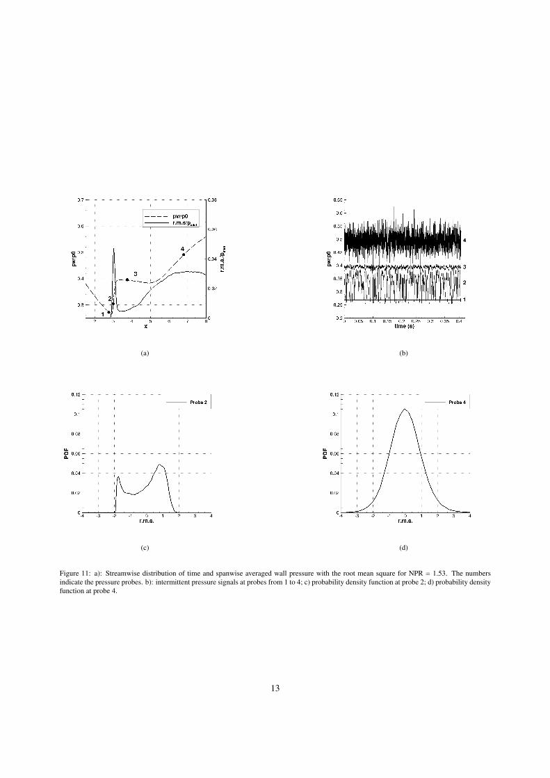
the other NPR’s very similar. These signals are taken from the numerical probes displayed in figure 11a. The firstprobe is located upstream the flow separation and its signal is almost constant in time, since this zone is the URANSdomain (attached boundary layer). The second probe is located in the region where there is the maximum valueof root mean square of the pressure oscillation, that is the region of the shock excursion. As shown in figure 11c,the probability density function of wall pressures is bimodal, this being a characteristics of an intermittent signal.In facts, the wall pressure alternates between two different ranges: that of the attached boundary layer and that ofthe turbulent flow downstream of the separation shock, spending less time near the mean value which falls betweenthe two extrema [30]. Thus there are two maxima in the probability curve. The first peak is associated with theprobability of finding pw in the narrow range of pressure associated with the attached boundary layer, hence showinga sharp peak. The latter peak has a broader maximum, that reflects the probability of finding pw in the wider range ofpressures that can be found downstream of the shock wave. The probe number 3 collects the signal at the beginningof the recirculating flow, which is characterized by a lower value of the oscillation amplitude with respect to theothers. Finally, the probe number 4 is located in the region of the vortex shedding, its signal shows a large oscillationamplitude and the probability density function is Gaussian, as shown in figure 11.

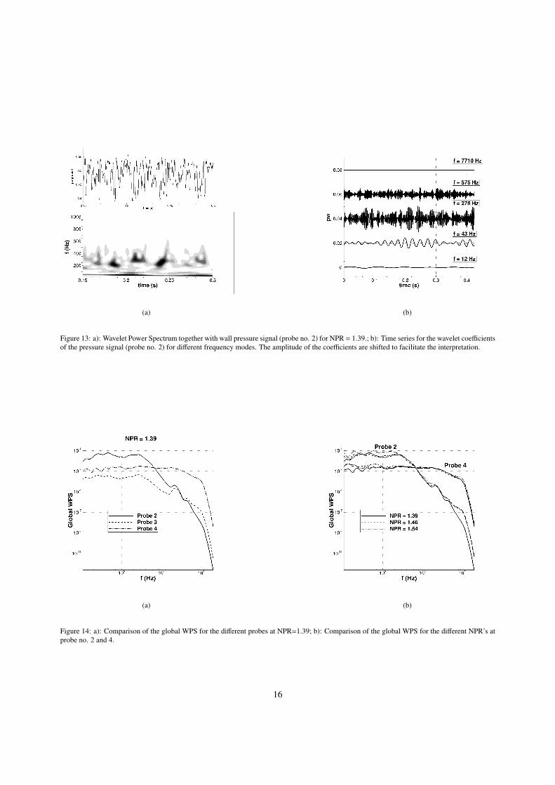
The wavelet power spectrum of the wall pressure signals describes how the variance σ2 of the wall pressure isdistributed in frequency, as described by equation (10). Figure 12a shows the normalized wavelet power spectrum|Wn(s)|2/σ2 in the frequency-time plane for the time series of the wall pressure from the second probe of the caseat NPR = 1.39. The normalization by 1/σ2 gives a measure of the power relative to the white noise [36]. The firstaspect that can be extracted from this plot is that the spectrum appears as a collection in time of events, characterizedby a variation of the amplitude of the oscillation energy and a variation of the frequency of the most energetic events.For example, it is possible to see an important event at 0.18 s with a characteristic frequency around 220 Hz, thena second event at 0.21 s with an increase in frequency (around 300 Hz) and a third event at 0.24 s with a frequencyof 250 Hz. Therefore it can be inferred from the data, that the shock movement is not continuous in time but ratherintermittent. This aspect can be better appreciated in figure 13a which shows an enlargement of the wavelet powerspectrum of the pressure signal from probe no. 2 between 0.15 s and 0.30 s, together with the pressure signal itself.It is evident from the picture that the pressure oscillation has an amplitude modulation, which is well captured by thewavelet power spectrum. To provide a better qualitative description of the dominant frequency modes within each ofthe main frequency branches, figure 13b shows the time series of a selection of the wavelet coefficients for differentfrequency modes. The time series, in fact, can be reconstructed by summing the real parts of the wavelet transformover all the scales:

pw(n) =δ jδt1/2

Cδψ0(0)

J∑j=0

R[Wn(s j)]

s1/2j

(13)

From this picture it can be seen that the more relevant contributions come from frequencies between 50 Hz and 600Hz, being the component at 278 Hz the most important. In addition, it is also possible to appreciate the amplitudemodulation of the various components. These findings highlight the importance of an accurate time-frequency waveletanalysis in addition to the classical Fourier spectral analysis, since the energy and frequency fluctuations are notobservable by means of the latter, that presents only time average information.

12

(a) (b)

(c) (d)

Figure 11: a): Streamwise distribution of time and spanwise averaged wall pressure with the root mean square for NPR = 1.53. The numbersindicate the pressure probes. b): intermittent pressure signals at probes from 1 to 4; c) probability density function at probe 2; d) probability densityfunction at probe 4.

13

Figure 12b shows the global wavelet power spectrum, that is the WPS integrated in time:

W2(s) =1N

N−1∑n=0

|Wn(s)|2 (14)

while figure 12c shows the global energy density E(s) =W2(s)

s jas a function of the scale. This last form is equivalent

to the compensated spectra in the classical Fourier analysis. In this way, it is possible to identify the scales mostcontributing to the energy, being possible to write [36]:

σ2 =δ jδtCδ

J∑j=0

E(s) (15)

From figure 12c it can be seen that there is a energy bump at large temporal scales (low frequencies), with a max-imum at 278 Hz. Therefore, the shock movement seems to be characterized by a broadband motion rather than bya sinusoidal motion. It may be worth full to recall that the frequency which gives the maximum value should beinterpreted in a statistical sense, that is as the most probable frequency. The analysis of the pressure signal from theprobe 3 (located at the beginning of the recirculation bubble) is reported in figures 12d, 12e and 12f. Most of theenergy is still located at low frequencies (lower than 1000 Hz) with an important bump at 278 Hz and a secondarybump at 2226 Hz. This second bump comes from integration in time of the intermittent events which can be seen inthe frequency-time space between 2000 and 2500 Hz and it is linked to the vortex shedding of the shear layer. Figures12g, 12h and 12i represent the spectral analysis of the fourth probe, located in the vortex shedding region. The energydensity now indicates that most of the energy is spread at higher frequencies, with a most probable frequency of 2647Hz. In this region dominates the three dimensional vortical structures, even if there is still a energy contribution fromthe lower frequencies (below 1000 Hz). Figure 14a compares the global wavelet power spectrum for all the pressureprobes at NPR = 1.39, in order to quantify the shifting of the energy from the lower frequencies, characterizing theshock excursion region, to the higher frequencies which characterize the turbulent recirculating region. This pictureis qualitatively the same shown by the Fourier analysis. The comparison of the global WPS for the different NPR’sat pressure probes no. 2 and 4 are shown in figure 14b. It can be seen that, qualitatively, the behavior of the spectraare very similar. While, from a quantitative point of view, the signals from probe no. 2 show that NPR=1.54 hasthe highest power at low frequencies. This is correlated to the highest shock intensity of this NPR. The signals fromprobe no. 4, instead, are similar also from a quantitative point of view, indicating the same behavior for the turbulentseparated region.

Finally, figure 15 compares the values of the frequencies characterizing the shock movement obtained with waveletand Fourier analysis with those taken from the Fourier analysis of the experimental data[10] (open symbols). The testcase with the isentropic Mach number equal to 1.34 is the only one which falls in the experimental range of shockMach numbers [10] Ms (1.280 ≤ MS ≤ 1.347). The computed value result to be in reasonable agreement withthe experimental ones, although the characteristic frequencies are sightly overestimated. We can speculate that suchdiscrepancy might be ascribed to some differences between the experiment and the simulations, as the presence ofside walls and suction slots employed in the experimental configuration to remove the boundary layer.

5. Conclusions

Delayed detached eddy simulations (DDES) of a planar nozzle with flow separation have been carried out fora Reynolds number, based on stagnation chamber properties and throat height, equal to 1.5 · 106 and for differentnozzle pressure ratios (or equivalently different isentropic Mach numbers). The nozzle flow simulated in this studyis characterized by a separation shock with a classical lambda shape and by an important recirculation zone, whichextends for several nozzle throat heights. All the simulations were able to capture a self-sustained unsteadiness of theshock system. As a first step, a classical statistical description of this unsteadiness has been carried out. The shockregion is characterized by a well defined peak in the root mean square distribution of the oscillating wall pressure.The amplitude of this peak increases with increasing Mach number. The evaluation of the intermittency factor hasallowed to evaluate the shock excursion length, which can reach the 20% of the throat height. All these findings

14

(a) WPS/σ2 at probe no. 2 (b) Global WPS at probe no. 2 (c) Global WPS/scale at probe no. 2

(d) WPS/σ2 at probe no. 3 (e) Global WPS at probe no. 2 (f) Global WPS/scale at probe no. 3

(g) WPS/σ2 at probe no. 4 (h) Global WPS at probe no. 2 (i) Global WPS/scale at probe no. 4

Figure 12: Wavelet Power Spectrum, global spectrum and global spectrum divided by the scale (energy density) of the pressure signals for NPR =

1.39.

15

(a) (b)

Figure 13: a): Wavelet Power Spectrum together with wall pressure signal (probe no. 2) for NPR = 1.39.; b): Time series for the wavelet coefficientsof the pressure signal (probe no. 2) for different frequency modes. The amplitude of the coefficients are shifted to facilitate the interpretation.

(a) (b)

Figure 14: a): Comparison of the global WPS for the different probes at NPR=1.39; b): Comparison of the global WPS for the different NPR’s atprobe no. 2 and 4.

16

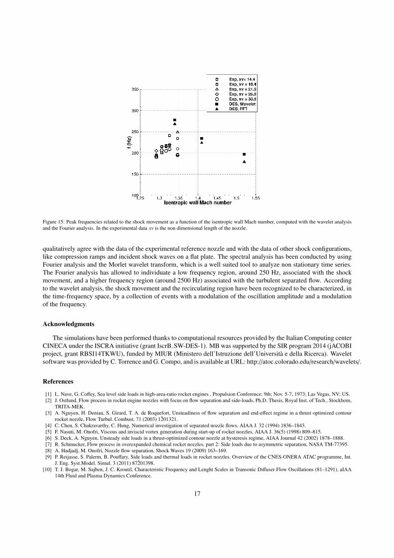
Figure 15: Peak frequencies related to the shock movement as a function of the isentropic wall Mach number, computed with the wavelet analysisand the Fourier analysis. In the experimental data xv is the non dimensional length of the nozzle.

qualitatively agree with the data of the experimental reference nozzle and with the data of other shock configurations,like compression ramps and incident shock waves on a flat plate. The spectral analysis has been conducted by usingFourier analysis and the Morlet wavelet transform, which is a well suited tool to analyze non stationary time series.The Fourier analysis has allowed to individuate a low frequency region, around 250 Hz, associated with the shockmovement, and a higher frequency region (around 2500 Hz) associated with the turbulent separated flow. Accordingto the wavelet analysis, the shock movement and the recirculating region have been recognized to be characterized, inthe time-frequency space, by a collection of events with a modulation of the oscillation amplitude and a modulationof the frequency.

Acknowledgments

The simulations have been performed thanks to computational resources provided by the Italian Computing centerCINECA under the ISCRA initiative (grant IscrB SW-DES-1). MB was supported by the SIR program 2014 (jACOBIproject, grant RBSI14TKWU), funded by MIUR (Ministero dell’Istruzione dell’Universita e della Ricerca). Waveletsoftware was provided by C. Torrence and G. Compo, and is available at URL: http://atoc.colorado.edu/research/wavelets/.

References

[1] L. Nave, G. Coffey, Sea level side loads in high-area-ratio rocket engines , Propulsion Conference; 9th; Nov. 5-7, 1973; Las Vegas, NV; US.[2] J. Ostlund, Flow process in rocket engine nozzles with focus on flow separation and side-loads, Ph.D. Thesis, Royal Inst. of Tech., Stockhom,

TRITA-MEK.[3] A. Nguyen, H. Deniau, S. Girard, T. A. de Roquefort, Unsteadiness of flow separation and end-effect regime in a thrust optimized contour

rocket nozzle, Flow Turbul. Combust. 71 (2003) 1201321.[4] C. Chen, S. Chakravarthy, C. Hung, Numerical investigation of separated nozzle flows, AIAA J. 32 (1994) 1836–1843.[5] F. Nasuti, M. Onofri, Viscous and inviscid vortex generation during start-up of rocket nozzles, AIAA J. 36(5) (1998) 809–815.[6] S. Deck, A. Nguyen, Unsteady side loads in a thrust-optimized contour nozzle at hysteresis regime, AIAA Journal 42 (2002) 1878–1888.[7] R. Schmucker, Flow process in overexpanded chemical rocket nozzles, part 2: Side loads due to asymmetric separation, NASA TM-77395.[8] A. Hadjadj, M. Onofri, Nozzle flow separation, Shock Waves 19 (2009) 163–169.[9] P. Reijasse, S. Palerm, B. Pouffary, Side loads and thermal loads in rocket nozzles. Overview of the CNES-ONERA ATAC programme, Int.

J. Eng. Syst.Model. Simul. 3 (2011) 87201398.[10] T. J. Bogar, M. Sajben, J. C. Kroutil, Characteristic Frequency and Lenght Scales in Transonic Diffuser Flow Oscillations (81–1291), aIAA

14th Fluid and Plasma Dynamics Conference.

17

[11] K. B. M. Q. Zaman, M. D. Dahl, T. J. Bencic, C. Y. Loh, Investigation of a transonic resonance’ with convergent divergent nozzles, Journalof Fluid Mechanics 463 (2002) 313–343. doi:10.1017/S0022112002008819.URL http://www.journals.cambridge.org/abstract_S0022112002008819

[12] T. Handa, M. Masuda, K. Matsuo, Mechanism of Shock Wave Oscillation in Transonic Diffusers, AIAA Journal 41 (1) (2003) 64–70.doi:10.2514/2.1914.

[13] A. D. Johnson, D. Papamoschou, Instability of shock-induced nozzle flow separation, Physics of Fluids 22 (1) (2010) 1–13. doi:10.1063/1.862466.

[14] S. Deck, Delayed detached eddy simulation of the end-effect regime and side-loads in an overexpanded nozzle flow, Shock Waves 19 (3)(2009) 239–249. doi:10.1007/s00193-009-0199-5.

[15] B. J. Olson, S. K. Lele, A mechanism for unsteady separation in over-expanded nozzle flow, Physics of Fluids 25 (11) (2013) 110809.doi:10.1063/1.4819349.URL http://scitation.aip.org/content/aip/journal/pof2/25/11/10.1063/1.4819349

[16] N. T. Clemens, V. Narayanaswamy, Low-Frequency Unsteadiness of Shock Wave/Turbulent Boundary Layer Interactions, Annual Review ofFluid Mechanics 46 (September) (2014) 469–492. doi:10.1146/annurev-fluid-010313-141346.URL http://www.annualreviews.org/doi/abs/10.1146/annurev-fluid-010313-141346

[17] P. J. Barnhart, I. Greber, Experimental Investigation of Unsteady Shock Wave Turbulent Boundary Layer Interactions About a Blunt Fin,Nasa Contractor Report 202334.

[18] M. Farge, Wavelet Transforms and Their Applications to Turbulence, Annu. Rev. Fluid Mech. 24 (1992) 395–457.[19] P. R. Spalart, Detached-Eddy Simulation, Annual Review of Fluid Mechanics 41 (1) (2009) 181–202. doi:10.1146/annurev.fluid.

010908.165130.[20] P. Spalart, S. Deck, M. Shur, K. Squires, M. Strelets, A. Travin, A new version of detached-eddy simulation, resistant to ambiguous grid

densities, Theor. Comput. Fluid Dyn. 20 (2006) 181–195.[21] P. Spalart, W. Jou, M. Strelets, S. Allmaras, Comments on the feasibility of les for wings, and on a hybrid rans/les approach, in: Advances in

DNS/LES, Greyedn Press, 1997, pp. 137–147.[22] S. Deck, Recent improvements in the zonal detached eddy simulation (ZDES) formulation, Theor. Comput. Fluid Dyn. 26 (2012) 523–550.[23] S. Pirozzoli, Numerical methods for high-speed flows, Annu. Rev. Fluid Mech. 43 (2011) 163–194.[24] F. Ducros, V. Ferrand, F. Nicoud, D. Darracq, C. Gacherieu, T. Poinsot, Large-eddy simulation of the shock/turbulence interaction, J. Comput.

Phys. 152 (1999) 5172013549.[25] M. Bernardini, S. Pirozzoli, A general strategy for the optimization of runge–kutta schemes for wave propagation phenomena, J. Com-

put. Phys. 228 (2009) 4182–4199.[26] T. A. Driscoll, S. A. Vavasis, Numerical Conformal Mapping Using Cross-Ratios and Delaunay Triangulation, SIAM Journal on Scientific

Computing 19 (6) (1998) 1783. doi:10.1137/S1064827596298580.URL http://link.aip.org/link/SJOCE3/v19/i6/p1783/s1&Agg=doi

[27] R. H. Stark, Flow Separation in Rocket Nozzles, a Simple Criteria (05–3940), 41st AIAA/ASME/SAE/ASEE Joint Propulsion Conference &Exhibit Tucson, Arizona.

[28] Y. Dubief, F. Delcayre, On coherent-vortex identification in turbulence, Journal of Turbulence 1 (2000) 1–22. doi:10.1088/1468-5248/1/1/011.URL http://www.tandfonline.com/doi/abs/10.1088/1468-5248/1/1/011

[29] P. Dupont, C. Haddad, J. F. Debieve, Space and time organization in a shock-induced separated boundary layer, Journal of Fluid Mechanics559 (2006) 255. doi:10.1017/S0022112006000267.

[30] D. S. Dolling, C. T. Or, Unsteadiness of the shock wave structure in attached and separated compression ramp flows, Experiments in Fluids3 (1) (1985) 24–32. doi:10.1007/BF00285267.

[31] K. Konno, T. Ohmachi, Ground-motion characteristics estimated from spectral ratio between horizontal and vertical components of mi-crotremor, Bulletin of the Seismological Society of America 88 (1) (1998) 228–241.

[32] T. Hsieh, T. J. Coakley, Downstream Boundary Effects on the Frequency of Self-excited Ocillations in Transonic Diffuser Flows (87–0161),aIAA 25th Aerospace Sciences Meeting.

[33] G. Aubard, X. Gloerfelt, J. Robinet, Large-eddy simulation of broadband unsteadiness in a shock/boundary-layer interaction, AIAA J. 51(2013) 2395–2409.

[34] I. Bermejo-Moreno, L. Campo, J. Larsson, J. Bodart, D. Helmer, J. K. Eaton, Confinement effects in shock wave/turbulent boundary layerinteractions through wall-modelled large-eddy simulations, Journal of Fluid Mechanics 758 (2014) 5–62. doi:10.1017/jfm.2014.505.URL http://journals.cambridge.org/abstract_S0022112014005059

[35] S. Pirozzoli, J. Larsson, J. Nichols, M. Bernardini, B. Morgan, S. Lele, Analysis of unsteady effects in shock/boundary layer interactions,Proceedings of the 2010 CTR summer program, Stanford University (2010).

[36] C. Torrence, G. P. Compo, A Practical Guide to Wavelet Analysis, Bulletin of the American Meteorological Society 79 (1) (1998) 61–78.doi:10.1175/1520-0477(1998)079<0061:APGTWA>2.0.CO;2.

18