Novi Sad J. Math. Vol. XX, No. Y, 20ZZ, ??-?? 2016 · 2016 Novi Sad J. Math. Vol. XX, No. Y, 20ZZ,...
23
First online - August 25, 2016. Draft version - November 2, 2016 Novi Sad J. Math. Vol. XX, No. Y, 20ZZ, ??-?? L ´ EVY PROCESSES, SUBORDINATORS AND CRIME MODELLING Tijana Levajkovi´ c 12 , Hermann Mena 1 and Martin Zarfl 1 Abstract. We investigate some properties of L´ evy processes in the context of subordinators. L´ evy walks can be represented as subordina- tors of random walks and L´ evy flights are random walks with trajectories composed of self-similar jumps. L´ evy processes provide a framework for modelling many physical phenomena. In this paper we consider, as an illustration, crime models based on Brownian motion and L´ evy flights. We propose an efficient implementation of the models by using high per- formance computing techniques. Numerical simulations on different sce- narios allows us to analyze some properties of the processes, particularly regimes of aggregation and first passage time. AMS Mathematics Subject Classification (2010): 60G51; 91D10; 60J60; 60G50 Key words and phrases: L´ evy processes; subordinators; random walks; L´ evy flight; first passage time; crime modelling 1. Introduction Applications of probability theory and stochastic processes arise in science and engineering, e.g. quantum mechanics, finance, biomathematics, etc. For example, in financial mathematics modelling fluctuations rely on L´ evy pro- cesses. L´ evy processes are stochastic processes with stationary and independent increments properties which satisfy a mild sample path regularity condition [1]. They are examples of random motion whose sample paths are right-continuous and have at most countable number of random jump discontinuities occurring at random times, on each finite time interval. Semimartingales and Markov processes are special subclasses of L´ evy processes, which include a number of very important processes: Brownian motion, Poisson process, stable and self- decomposable processes and subordinators [18]. Precisely, Brownian motion and homogeneous Poisson process appear in models of finance and insurance. The key difference between these two processes lies in the sample path behav- ior, Brownian motion has continuous sample paths whereas Poisson process is a counting process, a jump process. L´ evy flight is a class of random walks that is characterized by a heavy tailed step length distribution [13]. 1 Department of Mathematics, Faculty of Mathematics, Computer Science and Physics, University of Innsbruck, Austria, e-mail: [email protected], [email protected] and M.Zarfl@student.uibk.ac.at 2 Faculty of Traffic and Transport Engineering, University of Belgrade, Serbia e-mails: [email protected]
Transcript of Novi Sad J. Math. Vol. XX, No. Y, 20ZZ, ??-?? 2016 · 2016 Novi Sad J. Math. Vol. XX, No. Y, 20ZZ,...

Fir
ston
lin
e-
Au
gu
st25
,20
16.
Dra
ftve
rsio
n-
Nov
emb
er2,
2016
Novi Sad J. Math.Vol. XX, No. Y, 20ZZ, ??-??
LEVY PROCESSES, SUBORDINATORSAND CRIME MODELLING
Tijana Levajkovic12, Hermann Mena1and Martin Zarfl1
Abstract. We investigate some properties of Levy processes in thecontext of subordinators. Levy walks can be represented as subordina-tors of random walks and Levy flights are random walks with trajectoriescomposed of self-similar jumps. Levy processes provide a framework formodelling many physical phenomena. In this paper we consider, as anillustration, crime models based on Brownian motion and Levy flights.We propose an efficient implementation of the models by using high per-formance computing techniques. Numerical simulations on different sce-narios allows us to analyze some properties of the processes, particularlyregimes of aggregation and first passage time.
AMS Mathematics Subject Classification (2010): 60G51; 91D10; 60J60;60G50
Key words and phrases: Levy processes; subordinators; random walks;Levy flight; first passage time; crime modelling
1. Introduction
Applications of probability theory and stochastic processes arise in scienceand engineering, e.g. quantum mechanics, finance, biomathematics, etc. Forexample, in financial mathematics modelling fluctuations rely on Levy pro-cesses. Levy processes are stochastic processes with stationary and independentincrements properties which satisfy a mild sample path regularity condition [1].They are examples of random motion whose sample paths are right-continuousand have at most countable number of random jump discontinuities occurringat random times, on each finite time interval. Semimartingales and Markovprocesses are special subclasses of Levy processes, which include a number ofvery important processes: Brownian motion, Poisson process, stable and self-decomposable processes and subordinators [18]. Precisely, Brownian motionand homogeneous Poisson process appear in models of finance and insurance.The key difference between these two processes lies in the sample path behav-ior, Brownian motion has continuous sample paths whereas Poisson process isa counting process, a jump process. Levy flight is a class of random walks thatis characterized by a heavy tailed step length distribution [13].
1Department of Mathematics, Faculty of Mathematics, Computer Science and Physics,University of Innsbruck, Austria, e-mail: [email protected],[email protected] and [email protected]
2Faculty of Traffic and Transport Engineering, University of Belgrade, Serbiae-mails: [email protected]

Fir
ston
lin
e-
Au
gust
25,
2016.
Dra
ftve
rsio
n-
Nov
emb
er2,
2016
2 T. Levajkovic, H. Mena, M. Zarfl
Levy processes have an important role in modelling social behavior, urbanevolution, phenomena and processes appearing in biology and natural sciences.They appear, for example in predator-pray models, foraging patterns of animals[23], plasma physics and cell science [7], solute transport in heterogeneous media[24], social aspects, financial models [10], crime models [6, 22] etc.
Simple random walks models, also known as gambler ruin models, are usedto approximate one dimensional diffusions, such as Brownian motion, wherephysical particle is exposed to a great number of molecular collisions whichproduce random motion. The variance of diffusion is scaled linearly with time.Moreover, the Central limit theorem can be applied to random walks withoutlong-term correlations [8]. In this paper we focus on Levy flights, stable purejump Levy processes, which model anomalous diffusions, i.e. the diffusionphenomena whose variance is not linear. The nonlinearity of variance is dueto non Gaussian power-law tails of the probability distribution function, i.e.they are of the form tγ , γ 6= 1. Fractional diffusion equations are widely usedto describe anomalous diffusion processes [20, 25]. Especially, Levy walks areLevy flights with finite velocity. The first found super diffusion phenomenon isa fractional Brownian motion. The variance of fractional Brownian motion withthe Hurst parameter H ∈ (0, 1) can be related to the power scaling exponent,i.e. t2H . For H = 1
2 we retain a standard Brownian motion. In [11] theauthors showed how a power law truncated Levy stable distribution evolves intime to a distribution with power law asymptotics. Subordination of a processby another one, also called random time-change, is a technique from stochasticanalysis widely used for constructing new Markov processes or strongly conti-nuous semigroups [18]. It was first introduced by Bochner. We study simplerandom walks, continuous-time random walks and Levy flights, where in thesubordination a new operational time scale is used to measure the time betweentwo steps of the random walk.
In the class of Levy processes that can be written as Brownian motion timechanged by independent Levy subordinator, a question concerning the preciserelation between the standard first passage time arise [12]. The first passagetime, also called the hitting time, is the time at which a given process reachesa given subset of the state space. The first passage time is also referred as theinverse subordinator [26]. Exit times and return times are also examples ofhitting times [8]. First passage problems arise in financial mathematics, e.g.credit risk modelling, pricing barrier options etc. They also arise in the studyof fractional kinetics and the scaling limits of continuous random walks [26].
In this paper, we investigate the properties of different classes of Levy pro-cesses that are applied for modelling crime. Following [6, 22], we propose anefficient implementation of the models by using high performance computingtechniques, in particular we speed up simulations of the Levy flight model [6]by using MEX functions. This allows us to perform simulations of the Levymodel at the computational cost of the Brownian motion based model, makingfeasible to simulate crime modelling and other real life applications. We alsodiscuss several regimes of aggregation, like hotspots of high criminal activityand we provide a study of the fist passage time. In addition we generalize the

Fir
ston
lin
e-
Au
gust
25,
2016.
Dra
ftve
rsio
n-
Nove
mbe
r2,
2016
Levy processes, subordinators and crime modelling 3
one dimensional Levy flight model proposed in [6] to a two dimensional one al-lowing a detailed comparison with the model based on Brownian motion. Thelatter together with the efficient implementation are the main contributions ofthis paper. We point out that the same ideas can be applied straightforwardto other applications in financial mathematics or biology.
A strategy for the police to adapt dynamically to changing crime patternshas been introduced in [29]. The authors use optimization techniques to solvethe problem numerically. In case when the resulting model is linear (or can belinearized), a linear quadratic control problem approach can be used makingthe computation with real data feasible as efficient numerical solvers have beenproposed, e.g. [2, 3, 4, 16]. The latter we intend to investigate in our futurework.
The paper is organized as follows: in Section 2 we present a brief overviewof Levy processes, subordinators and random walks. Then, in Section 3 wedescribe the crime models for burglar locomotion. Afterwards, in Section 4we perform numerical simulations for different scenarios and we study the firstpassage time. Finally, in Section 5 we present some conclusions.
2. Theoretical background
2.1. Levy processes
Consider a complete probability space (Ω,F ,P) equipped with a filtration(Ft)0≤t≤T , T > 0. The σ-algebra FT represents the information available inthe model up to time T . A real valued stochastic process X = Xt(ω) = (Xt)t≥0
defined on (Ω,F ,P) is called an one dimensional Levy process if X0 = 0 a.s.,X has independent and stationary increments and X is stochastically continu-ous. Both Brownian motion and Poisson process are temporary homogeneousLevy processes, i.e. the probability distribution of the increment Xt+h − Xt,for h > 0 is independent of t. Almost all trajectories of Brownian motion arecontinuous, while those of Poisson process are discontinuous, and they increaseonly by jumps of unit magnitude. Other important examples of Levy pro-cesses are compound Poisson process, Gamma process, α-stable processes, selfdecomposable processes.
A real valued random variable Y has an infinitely divisible distribution iffor each n ∈ N there exist a sequence of independent identically distributedrandom variables Y1,n, ..., Yn,n such that Y and Y1,n + ... + Yn,n have equaldistribution. Hence, the probability law µ of a real valued random variableis infinitely divisible if it can be decomposed to n-fold convolution µ = µ∗nn ,n ∈ N, for some probability law µn. The characteristic exponent of a randomvariable Y is defined by
Ψ(u) = − logE(eiuY ), u ∈ R.
Therefore, Y has an infinitely divisible distribution if for all n ∈ N thereexists a characteristic exponent Ψn of a probability distribution such that
Fir
ston
lin
e-
Au
gust
25,
2016.
Dra
ftve
rsio
n-
Nov
emb
er2,
2016
4 T. Levajkovic, H. Mena, M. Zarfl
Ψ(u) = nΨn(u), u ∈ R. Complete characterization of an infinitely divisible dis-tribution in terms of its characteristic exponent is given by the Levy-Khintchineformula [1, 21]
Theorem 2.1 (The Levy-Khintchine formula). The probability law µ of a realvalued random variable is infinitely divisible with the characteristic exponent Ψ
(2.1)
∫Reiθx µ(dx) = e−Ψ(θ), θ ∈ R
if and only if there exists the triplet (a, σ,Π), where a ∈ R, σ ≥ 0 and Π is theLevy measure, i.e. the measure concentrated on R \ 0 which satisfies
(2.2)
∫R
(1 ∧ x2) Π(dx) < ∞,
such that
(2.3) Ψ(θ) = iaθ +1
2σ2θ2 +
∫R
(1− eiθx + iθx1|x|<1) Π(dx), θ ∈ R.
The proof of the Levy-Khintchine formula can be found, for example in [1, 21].It is clear that every Levy process can be related to some infinite divisi-
ble distribution. If X is a Levy process, then Xt has an infinitely divisibledistribution for each t ≥ 0. Moreover, for every infinite divisible process, itis possible to construct a Levy process Xt so that X1 has the given infinitedivisible distribution. This is the statement of the following theorem.
Theorem 2.2. Given a triplet (a, σ,Π), where a ∈ R, σ ≥ 0 and Π is the Levymeasure such that (2.2) is satisfied. Then there exists a unique Levy process Xsuch that (2.1) and (2.3) hold.
Note that every Levy process can be decomposed into the sum of threeterms. The first term, seen as a continuous part of a Levy process is representedby a Brownian motion with drift, the second term represents a compensatedsum of small jumps, while the third term describes the large jumps and isrepresented by compound Poisson process.
2.1.1. Subordinators
Levy processes with almost sure nondecreasing paths are called subordinators.Such processes can be thought of as random models of time evolution. Theircharacteristic exponent (2.3) is of the form
Ψ(θ) = iaθ +
∫ +∞
0
(1− eixθ) Π(dx) .
A wide class of Levy processes appearing in applications is obtained by subor-dination of Brownian motion with drift [14, 18].
Fir
ston
lin
e-
Au
gu
st25
,20
16.
Dra
ftve
rsio
n-
Nov
emb
er2,
2016
Levy processes, subordinators and crime modelling 5
Theorem 2.3. Let X = (Xt)t≥0 be a Levy process with the characteristicexponent Ψ and S = (Sτ )τ≥0 an independent subordinator defined on the sameprobability space as X with the characteristic exponent Φ. Then, the processYτ = (XSτ )τ≥0 is a Levy process with the characteristic exponent Φ Ψ.
The proof of the previous theorem can be found for example in [1, 15]. In [9]the authors suggested that the value of a risky asset can evolve as the processon an abstract time scale suitable to the rate of business translations called thebusiness (operational) time. The subordinator S represents the link betweenbusiness time and real time. Particularly, in the models of crime activities weare considering in Section 3, the position Y of the burglar at the certain timeis distributed by St and follows the process Yt = X St = XSt . This meansthat at real time t > 0, St units of business (”robbing”) time pass and thevalue of a burglar activity is positioned at XSt .
A stable Levy process is a Levy process X for which Xt is a stable randomvariable for all t ≥ 0. These processes are important in applications becausethey display the self-similarity property.
A random time τ taking values in [0,+∞) is a stopping time with respectto the process X if τ ≤ t ∈ Ft for all t ≥ 0. The σ-algebra associated withτ is defined by Fτ = B ∈ F : B ∩ τ ≤ t ∈ Ft, for all t ≥ 0. Stoppingtime can be seen as a random time that does not require knowledge about thefuture. From the available information we can only tell whether or not τ ≤ tholds [18].
Example 2.4. Let Bt, t ≥ 0 be a standard Brownian motion, σ > 0, θ > 0and S an independent subordinator. Then, Wt = σBt+θt, t ≥ 0 is a Brownianmotion with drift θ and scaling (dispersion) coefficient σ [14]. A subordinatedprocess BSt performs jumps in random time, where time is passing according toSt, t ≥ 0. For a linear transformation, when St = b2 t the process BSt = Bb2t,b 6= 0 is a Brownian motion with drift b2 and dispersion coefficient b.We subordinate Brownian motion and by time changing X = W S constructa Levy process Xt = WSt = σBSt + θSt. Let τ be a stopping time with respectto the process W . Define a process Yt = Wt+τ −Wτ , t ≥ 0. Then Y = (Yt)t≥0
is also a Brownian motion with the same drift and scale parameter.
The first hitting time, also called the first passage time and the inversesubordinator, is the time at which a given process reaches a given subset ofthe state space. Let (Ω,F ,P) be a given probability space and let M be ameasurable state space. Let X : Ω × [0,+∞) → M be a stochastic processand A a measurable subset of the state space M . Then, the first hitting timeτA : Ω→ [0,+∞) is the random variable defined by
τA(ω) = inft ≥ 0 : Xt(ω) ∈ A.
Any stopping time is a hitting time for a properly chosen process and target set.Precisely, the hitting time of a measurable set, for a progressively measurableprocess, is a stopping time. Progressively measurable processes include, inparticular, all right and left-continuous adapted processes. The converse also

Fir
ston
lin
e-
Au
gust
25,
2016.
Dra
ftve
rsio
n-
Nov
emb
er2,
2016
6 T. Levajkovic, H. Mena, M. Zarfl
holds, every stopping time defined with respect to a filtration over a real valuedtime index set can be represented by a hitting time [1]. The mean first passagetime is called the renewal function. All the moments of the first passage timecan be computed if the renewal function is first computed [26].
Example 2.5. For α ∈ (0, 1) and u ≥ 0 it holds
uα =α
Γ(1− α)
∫ +∞
0
(1− e−ux)dx
x1+α.
Thus, there exists α-stable subordinator S with the characteristic exponentΨ(u) = uα and the characteristics of S are (0, λ), where λ(dx) = α
Γ(1−α)dxx1+α .
Moreover, the renewal function for the α-stable subordinator is given by tα
Γ(α+1) .
The 12 -stable subordinator is called the Levy subordinator and its probabilistic
interpretation is the first hitting time for one dimensional Brownian motion Bt,i.e. St = infs > 0 : Bs = t√
2. Recall, the probability density function of a
random variable Sb√
2 = infs > 0 : Bs = b obtained by the reflection principle
is given in the close form |b|√2πt3
e−b2
2t . Moreover, for an α-stable subordinator
S independent on a Brownian motion B, the process Z = BSτ is rotationallyinvariant 2α-stable process. For more details we refer to [1, 14, 18, 26].
2.2. Fractional Laplacian
We recall briefly some facts on fractional discrete Laplace operator. LetZh = hj , j ∈ Z be a mesh on R of size h > 0. The discrete Laplacian ∆h isgiven by
−∆huj = − 1
h2(uj+1 − 2uj + uj−1),
where uj , j ∈ Z ia a function on Zh. The fractional discrete Laplacian (−∆h)s
is defined by
(−∆h)s uj =1
Γ(−s)
∫ ∞0
(et∆h uj − uj)dt
t1+s,
where vj(t) = et∆)h uj is the solution of the semidiscrete heat equation
∂t vj = ∆h vj , in Zh × (0,∞),
vj(0) = uj , on Zh.
2.3. Random walk
Random walk is a process by which randomly moving objects wander awayfrom where they started. The simplest random walk is an one dimensionalsimple random walk. Two or three dimensional random walks are commonlyfound in nature. For example, when gas particles bounce around in a room,changing direction every time they collide with another particle, it is randomwalk that determines how long it will take them to travel from one location toanother. The particles in a drop of ink added to water will spread out partially

Fir
ston
lin
e-
Au
gu
st25
,20
16.
Dra
ftve
rsio
n-
Nov
emb
er2,
2016
Levy processes, subordinators and crime modelling 7
due to a random walk [13]. For all random walks it holds that the total distancetraveled from where it started is approximately
√N , where N is the number
of steps taken. This is called the universal scaling property [8]. Random walkshave various interesting mathematical properties that vary depending on thedimension in which the walk occurs [5, 7, 13, 20].
Random walks generated by steps taken at regular intervals can be ge-neralized by introducing a probability density function for pausing times be-tween successive steps in the walk, i.e. the waiting time distribution [13].
2.3.1. Simple random walk
We recall briefly the concept of an one dimensional simple random walk [8, 13].The walker starts at the zero on a number line. It can move one step, in eachmoment of time, either forward or backward, with same probability. In thiscase only the current location of the walker determines the random motion, thepast is not relevant. The position of the walk after N steps can be representedas a sum of consecutive displacements ∆Xn, i.e.
(2.4) XN =
N∑i=1
∆Xi,
where ∆Xi are independent identically distributed random variables with thevariance σ2. Each displacement has the same probability density functionp(∆x). In the case of symmetric single step, from the strong law of large num-bers it follows that the average velocity vanishes, i.e. lim
N→∞XNN = E(∆X1) = 0,
where E is the expectation with respect to the measure P. Since the walkermakes large excursions both forward and backward, so that lim sup
N→∞XN = +∞,
lim infN→∞
XN = −∞ P-a.s. a random walker visits the origin, and any other inte-
ger point on the line, infinitely often. Fluctuations of the random walk can becharacterized by the Central limit theorem. The distribution of XN is asymp-totically normal with zero mean and variance σ2N . Clearly, the probabilitydensity function fY (y,N) for the scaled position YN = XN√
N= 1√
N
∑Ni=1 ∆Xi
is Gaussian and independent of N when N → ∞. Thus the universal scalingrelation for ordinary random walks XN ∼
√N follows and the probability
density function fX(x,N) for the position XN is asymptotically Gaussian.
Example 2.6. Brownian motion is a process that could be obtain as a limitof a simple random walk. Moreover, one dimensional Brownian motion can berepresented as a random Fourier series
Bt =
√2
π
∞∑n=0
sin (πt(n+ 12 ))
n+ 12
Zn,
for each t ≥ 0, where Zn, n ∈ N0 is a sequence of independent identicallydistributed standardized Gaussian random variables [1].
Fir
ston
lin
e-
Au
gust
25,
2016.
Dra
ftve
rsio
n-
Nov
emb
er2,
2016
8 T. Levajkovic, H. Mena, M. Zarfl
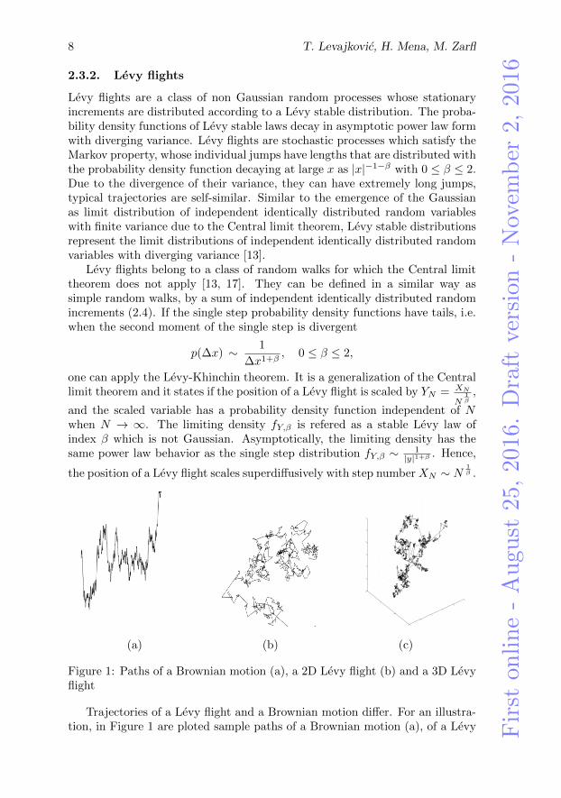
2.3.2. Levy flights
Levy flights are a class of non Gaussian random processes whose stationaryincrements are distributed according to a Levy stable distribution. The proba-bility density functions of Levy stable laws decay in asymptotic power law formwith diverging variance. Levy flights are stochastic processes which satisfy theMarkov property, whose individual jumps have lengths that are distributed withthe probability density function decaying at large x as |x|−1−β with 0 ≤ β ≤ 2.Due to the divergence of their variance, they can have extremely long jumps,typical trajectories are self-similar. Similar to the emergence of the Gaussianas limit distribution of independent identically distributed random variableswith finite variance due to the Central limit theorem, Levy stable distributionsrepresent the limit distributions of independent identically distributed randomvariables with diverging variance [13].
Levy flights belong to a class of random walks for which the Central limittheorem does not apply [13, 17]. They can be defined in a similar way assimple random walks, by a sum of independent identically distributed randomincrements (2.4). If the single step probability density functions have tails, i.e.when the second moment of the single step is divergent
p(∆x) ∼ 1
∆x1+β, 0 ≤ β ≤ 2,
one can apply the Levy-Khinchin theorem. It is a generalization of the Centrallimit theorem and it states if the position of a Levy flight is scaled by YN = XN
N1β
,
and the scaled variable has a probability density function independent of Nwhen N → ∞. The limiting density fY,β is refered as a stable Levy law ofindex β which is not Gaussian. Asymptotically, the limiting density has thesame power law behavior as the single step distribution fY,β ∼ 1
|y|1+β . Hence,
the position of a Levy flight scales superdiffusively with step numberXN ∼ N1β .
(a) (b) (c)
Figure 1: Paths of a Brownian motion (a), a 2D Levy flight (b) and a 3D Levyflight
Trajectories of a Levy flight and a Brownian motion differ. For an illustra-tion, in Figure 1 are ploted sample paths of a Brownian motion (a), of a Levy
Fir
ston
lin
e-
Au
gu
st25
,20
16.
Dra
ftve
rsio
n-
Nov
emb
er2,
2016
Levy processes, subordinators and crime modelling 9
flight of 1000 steps in two dimensions (b) and in three dimensions (c). Paths ofBrownian motion are continuous and almost nowhere differential. Each part ofthe path is again a trajectory of a Brownian motion [14]. On the other hand,Levy flight is characterized by many small moves combined with a few longertrajectories, i.e. longer rutes are taken on occasion. The characteristic size ofthe Levy flight is the size of the largest step and the flight is self- similar athigher magnifications [13].
2.3.3. Continuous time random walks
Temporally continuous random walks can be constructed from time discretesimple random walks by identifying the step number N with the time elapsedt and associated time increment ∆t = t
N between successive steps. A gene-ralization of this concept leads to the continuous time random walk [13]. Itssimple version is defined by two probability density functions, one for spa-tial displacements g1(∆x) and one for random temporal increments g2(∆t).Thus, continuous time random walk consists of pairwise random independentevents, spacial displacement ∆x and temporal increment ∆t and the probabilitydensity functions
p(∆x,∆t) = g1(∆x) g2(∆t).
After N steps, the position of the walker is given by XN =∑Ni=1 ∆xi and the
time elapsed is TN =∑Ni=1 ∆ti. The probability density function f(x, t) of the
position Xt after time t is calculated in [17].Particularly, the ordinary diffusion occurs when the variance of the spatial
steps and the expectation of the temporal increments exist. Then, the continu-ous time random walks are equivalent to Brownian motion on large spatio-temporal scales. When the spatial displacements are drawn from a power lawprobability density function and the temporal increment have finite expecta-tion, the continuous time random walk is equivalent to ordinary Levy flights
with a superdiffusive scaling with time Xt ∼ t1β . When the ordinary spatial
steps are combined with a power law in the probability density function, thetime between successive spatial increments can be very long, effectively slowingdown the random walk. In this case one obtains the scaling relation Xt ∼ t
α2 .
Since α < 1 these processes are subdiffusive and are refered to fractional Brow-niam motion.
Random walks in random environments are studied in [5].
3. Crime modelling as an application
In this section as an application of Levy proceses and Levy flights we discussdifferent models of criminal activity (residential burglaries where the targetsare stationary). In particular, we discuss models proposed in [6, 22]. The firstmodel, also called the UCLA model, describes the locomotion of criminal agentsby Brownian motion [22] and the second one is based on Levy flights motion[6]. The second model relies on the advantages of Levy distributed excursionlengths, which optimize the search compared to the Brownian search. The
Fir
ston
lin
e-
Au
gust
25,
2016.
Dra
ftve
rsio
n-
Nov
emb
er2,
2016
10 T. Levajkovic, H. Mena, M. Zarfl
considered models may be also applied for modelling processes appearing innature such as the foraging behavior of bacteria and animals or the spreadingof diseases [7, 23].
Due to social, economic, geographic structure the criminal activity is notdistributed uniformly. The regions with elevated criminal activities are calledhotspots. Different spatial-temporal methods for crime analysis were studied indetails in [19, 28]. In [22] the authors proposed a discrete model of the formationof hotspots of criminal activity based on a random walk biased toward theattractive burglary sites, such that the criminals can move only to adjacentcites in each time step. On the basis of the discrete system, a continuum modelis obtained as the limit of the discrete one. The continuous model is thusbased on biased Brownian motion and described by a system of coupled partialdifferential equations (PDEs) for criminal density and the attractiveness field.In [6] the authors assumed that criminals can make movements not only to theneighborhood sites, but also can exhibit a long range of jumps. The model isnonlocal and involves occasional long jumps spread with a local random walks,i.e. in its continuous version it involves a Levy flight motion. Criminals are ableto examine the potential robbery spots and have knowledge, beside their localenvironment, also of far away surroundings. In this case the continuous modelis governed by PDEs involving a fractional Laplace operator, which allows thesuperdiffusion of criminal density. Note that different mobility patterns aredue to different types of criminals [27].
Following [6, 22] we perform numerical simulations for different parameterchoices. This allows us to visualize several regimes of aggregation, like hotspotsof high criminal activity. In addition, we study the fist passage time. One ofthe contributions of this paper is to generalize the one dimensional Levy flightmodel proposed in [6] to a two dimensional one allowing a detailed comparisonwith the model based on Brownian motion.
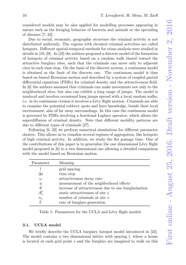
Parameter Meaning
l grid spacing∆t time stepω attractiveness decay rateη measurement of the neighborhood effectsθ increase of attractiveness due to one burglarisationA0s static attractiveness of site s
ns number of criminals at site sΓ rate of burglars generation
Table 1: Parameters for the UCLA and Levy flight models
3.1. UCLA model
We briefly describe the UCLA burglary hotspot model introduced in [22].The model contains a two dimensional lattice with spacing l, where a houseis located at each grid point s and the burglars are imagined to walk on this

Fir
ston
lin
e-
Au
gu
st25
,20
16.
Dra
ftve
rsio
n-
Nov
emb
er2,
2016
Levy processes, subordinators and crime modelling 11
lattice. Each house is assigned with an attractiveness As(t), which displays theburglars thinking of the value of the house as a burglary target. The model isbased upon the assumption, that the attractiveness is not modeled by proper-ties like value, security or location but rather with the broken windows effectand near-repeated victimization, where the broken windows effect explains thatthe inhibition threshold recedes due to previous burglaries. Therefore, the at-tractiveness is divided into two parts, a static part A0
s and the dynamic partBs(t). Thus,
As(t) = A0s +Bs(t).
The static parts A0s measures values like e.g. location and accessibility, whereas
the dynamic part Bs(t) changes through interactions with the burglars.In one time step a criminal agent can either decide to burglarize the housewhere he is located or move on to an adjacent site. The probability for theburglar to commit burglary in a time step of length ∆t is given by a standardPoisson process
(3.1) ps(t) = 1− e−As(t)∆t,
where the expected value of events is As(t)∆t. It is assumed that a criminalagent committed burglary, gets removed from the grid. Furthermore, burglarsare generated at each grid point with rate Γ. In the case that the burglardoes not burglarize, it moves to an adjacent site into direction of areas withhigh attractiveness. The locomotion of the criminal agents follows a Brownianmotion. Hence, the transition probability to move from a site s to an adjacentsite n is given by
(3.2) qs,n(t) =An(t)∑
s′∼sAs′(t)
,
with s′ ∼ s being all neighboring sites of s.The dynamic part of the attractiveness Bs(t) depends on former burglaries
at site s. Thus, Bs(t) is increased every time the house is getting burglarizedby a value θ. For this increment affecting the attractiveness only for a finitetime period the dynamic part is modeled by
(3.3) Bs(t+ ∆t) = Bs(t)(1− ω∆t) + θEs(t),
where Es(t) is the number of burglaries, ∆t is the timescale and ω representsthe decay rate of the dynamic attractiveness field. For letting the attractivenessspread over adjacent houses the dynamic part becomes
(3.4) Bs(t+ ∆t) =
[(1− η)Bs(t) +
η
z
∑s′∼s
Bs′(t)
](1− ω∆t) + θEs(t),
where z is the number of adjacent sites (four in two dimensions) and η ∈ [0, 1] isa parameter to measure near repeated victimization, higher value of η leads to

Fir
ston
lin
e-
Au
gust
25,
2016.
Dra
ftve
rsio
n-
Nov
emb
er2,
2016
12 T. Levajkovic, H. Mena, M. Zarfl
higher attractiveness generated by any burglary event, i.e. to more robberies.Rewriting (3.4) using the discrete Laplacian operator (see Section 2.2),
∆Bs(t) =1
l2·
(∑s′∼s
Bs′(t)− zBs(t),
)with l being the grid spacing leads to
(3.5) Bs(t+ ∆t) =
[Bs(t) +
ηl2
z∆Bs(t)
](1− ω∆t) + θEs(t).
Further we consider the simplest version of the discrete system (3.5), i.e. wewill obtain an homogeneous equilibrium solution. We assume that all sites havethe same attractiveness A and same number of criminals n on average. Moredetails are given in Section 4.
A continuous version of the discrete UCLA model is obtained as a limit ofthe discrete one. It corresponds to the reaction diffusion model of the form
∂B
∂t=ηD
zO2B − ωB + εDρA
∂ρ
∂t=D
z~O ·(~Oρ− 2ρ
A~OA
)− ρA+ γ
(3.6)
where ρ = ns(t)l2 , γ = Γ
l2 and fixed values D = l2
∆t and ε = θ∆t. In (3.6),the first equation gives the dynamics of the attractiveness and the second onethe criminal activity. The attractiveness diffuses throughout the environmentand simultaneously decays in time and reacts with criminals to create moreattractiveness [22].
3.2. Crime models with Levy flights
In [6] the authors presented an one dimensional approach for the locomotionof the criminal agents and suggested a model involving Levy flights. Allowingthe burglars to move via Levy flights, the burglars can search more efficientlyfor houses with high attractiveness by doing larger jumps. Thereby the distri-bution of step lengths obeys a power law. In this paper, we expand the modeldescribed in [6] to a two dimensional model. Moreover we compare the resultsof simulations of two dimensional UCLA and Levy flight models.
Each time step, every burglar in the system either choose to move from hislocation to a new site or to commit a crime. Burglars are appearing randomlywith the probability (3.1). Let Es(t) denote the number of crimes at each sites during the time interval (t, t+∆t) and Ns(t) the average number of criminalsat the site s in the time interval (t, t + ∆t). Then, the dynamic part of theattractiveness is given by (3.3).
The relative weight of a criminal moving from a site s = (s1, s2) to a differentsite s′ = (s′1, s
′2) is given by
(3.7) ws,s′ =As′
lµ‖s− s′‖µ=
As′
lµ√
(s1 − s′1)2 + (s2 − s′2)2µ ,
Fir
ston
lin
e-
Au
gu
st25
,20
16.
Dra
ftve
rsio
n-
Nov
emb
er2,
2016
Levy processes, subordinators and crime modelling 13
where µ is the exponent of the underlying power law for the Levy flight and lis the grid spacing. The transition probability qs,s′ for a burglar to move fromsite s to a different site s′ is then
(3.8) qs,s′ =ws,s′∑
r∈Z2,r 6=sws,r
.
As in the UCLA model, here is also assumed that during the time interval ∆tthe burglar either commits a crime or else moves on according to a biased flight.New criminals appear with the rate Γ. The modelling of the attractivenessfollows the same way as in the UCLA model.
Since the criminals can appear at the site s by moving there from some sites, as is governed by qs,s, or by the birth with Γ∆t, it follows
Ns(t+ ∆t) =∑
y∈Z, i 6=sNi (1−Ai∆t) · qi,s + Γ∆t.
The corresponding continuum version of the model is again reaction diffu-sion system that involves in this case the fractional Laplace operator, i.e.
∂A
∂t= ηAxx −A+ α+Aρ
∂ρ
∂t= D ·
(A(−∆)s (
ρ
A)− ρ
A(−∆)s (A)
)−Aρ+ β,
(3.9)
for a suitable choice of the parameters η = l2η2ω∆t , D = l2s
22s∆t
√π|Γ(−s)|
zωΓ(2s+1) , α = A0
ω
and β = Γθω2 . For more details on the derivation of the system (3.9) and its
stability properties we refer to [6].
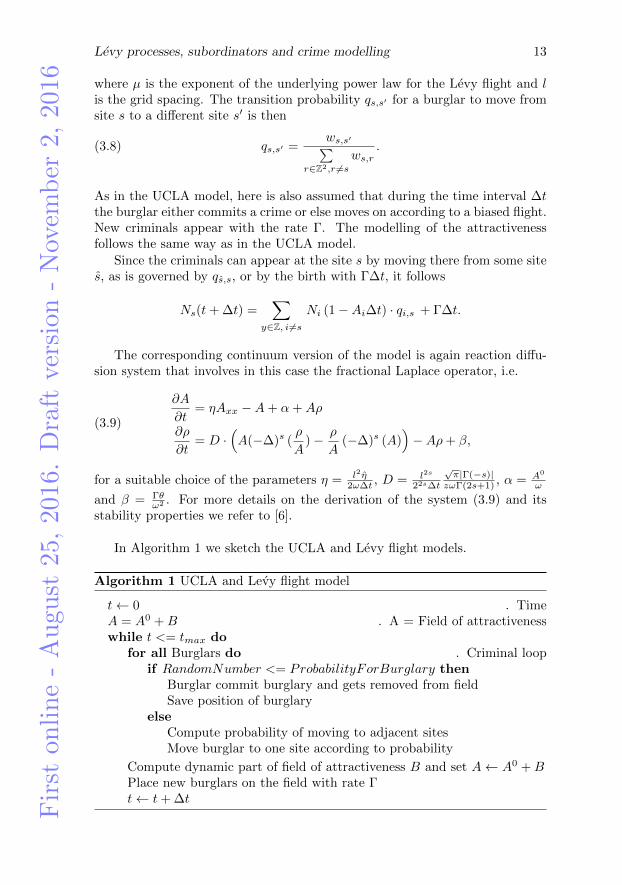
In Algorithm 1 we sketch the UCLA and Levy flight models.
Algorithm 1 UCLA and Levy flight model
t← 0 . TimeA = A0 +B . A = Field of attractivenesswhile t <= tmax do
for all Burglars do . Criminal loopif RandomNumber <= ProbabilityForBurglary then
Burglar commit burglary and gets removed from fieldSave position of burglary
elseCompute probability of moving to adjacent sitesMove burglar to one site according to probability
Compute dynamic part of field of attractiveness B and set A← A0 +BPlace new burglars on the field with rate Γt← t+ ∆t
Fir
ston
lin
e-
Au
gust
25,
2016.
Dra
ftve
rsio
n-
Nov
emb
er2,
2016
14 T. Levajkovic, H. Mena, M. Zarfl
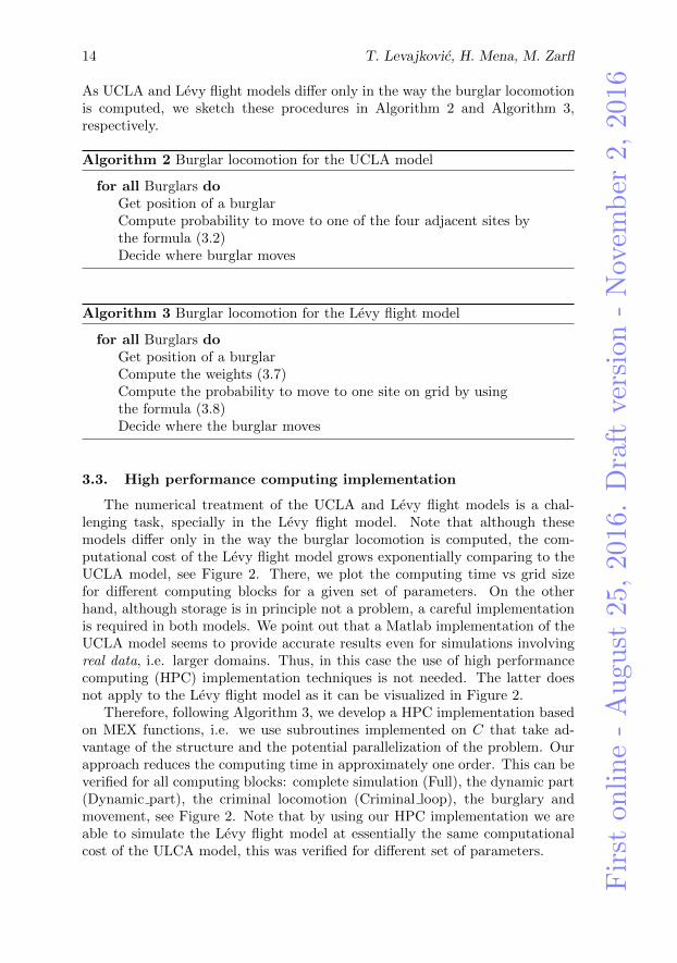
As UCLA and Levy flight models differ only in the way the burglar locomotionis computed, we sketch these procedures in Algorithm 2 and Algorithm 3,respectively.
Algorithm 2 Burglar locomotion for the UCLA model
for all Burglars doGet position of a burglarCompute probability to move to one of the four adjacent sites bythe formula (3.2)Decide where burglar moves
Algorithm 3 Burglar locomotion for the Levy flight model
for all Burglars doGet position of a burglarCompute the weights (3.7)Compute the probability to move to one site on grid by usingthe formula (3.8)Decide where the burglar moves
3.3. High performance computing implementation
The numerical treatment of the UCLA and Levy flight models is a chal-lenging task, specially in the Levy flight model. Note that although thesemodels differ only in the way the burglar locomotion is computed, the com-putational cost of the Levy flight model grows exponentially comparing to theUCLA model, see Figure 2. There, we plot the computing time vs grid sizefor different computing blocks for a given set of parameters. On the otherhand, although storage is in principle not a problem, a careful implementationis required in both models. We point out that a Matlab implementation of theUCLA model seems to provide accurate results even for simulations involvingreal data, i.e. larger domains. Thus, in this case the use of high performancecomputing (HPC) implementation techniques is not needed. The latter doesnot apply to the Levy flight model as it can be visualized in Figure 2.
Therefore, following Algorithm 3, we develop a HPC implementation basedon MEX functions, i.e. we use subroutines implemented on C that take ad-vantage of the structure and the potential parallelization of the problem. Ourapproach reduces the computing time in approximately one order. This can beverified for all computing blocks: complete simulation (Full), the dynamic part(Dynamic part), the criminal locomotion (Criminal loop), the burglary andmovement, see Figure 2. Note that by using our HPC implementation we areable to simulate the Levy flight model at essentially the same computationalcost of the ULCA model, this was verified for different set of parameters.

Fir
ston
lin
e-
Au
gu
st25
,20
16.
Dra
ftve
rsio
n-
Nov
emb
er2,
2016
Levy processes, subordinators and crime modelling 15
Full Dynamic_Part Criminal_Loop Burglary Movement
1e−02
1e+01
1e+04
1e−02
1e+01
1e+04
1e−02
1e+01
1e+04
1e−02
1e+01
1e+04
12
34
25 50 75 100125 25 50 75 100125 25 50 75 100125 25 50 75 100125 25 50 75 100125Size
Tim
e
Type
LEVY
LEVY_MEX
UCLA
Computation Time against Grid Size for different Parts and Parameter Choices
Figure 2: Computing time vs grid size for different parameter choices in themodels.
4. Numerical simulations
We perform numerical simulations for different choices of the parametersgiven in Table 1. In Subsection 4.2 we generalize the one dimensional Levy flightmodel proposed in [6] to a two dimensional one allowing a detailed comparisonwith the UCLA model from Subsection 4.1. A comparison of the burglar loco-motion is provided in Subsection 4.3. Finally, in Subsection 4.4 we present astudy of the first passage time.
All the experiments in this section were performed in Matlab. The valuetmax in Algorithm 1, represents the number of days that the simulation ran.Double-precision floating-point arithmetic was employed in all cases. An effi-cient implementation on C of the main routines was developed.
4.1. UCLA model
All simulations were performed with l = 1, ∆t = 1/100, ω = 1/15 andA0 = 1/30. The variation of the parameters η, θ and Γ can be seen in eachfigure description.
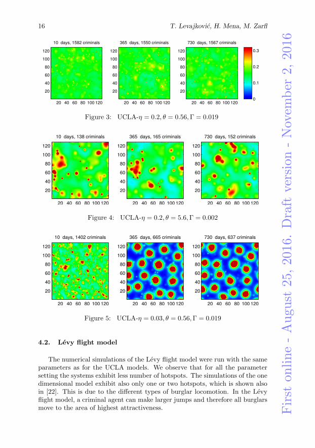
While in Figure 3 one can observe no hotspot forming, the other simulationsform hotspots in different ways. Figure 4 exhibit dynamic hotspots, whilst incontrary Figure 5 leads to static hotspots. Finally, Figure 6 form spatiallystatic hotspots with more deformations over time.
Fir
ston
lin
e-
Au
gust
25,
2016.
Dra
ftve
rsio
n-
Nov
emb
er2,
2016
16 T. Levajkovic, H. Mena, M. Zarfl
10 days, 1582 criminals
20 40 60 80 100 120
20
40
60
80
100
120
365 days, 1550 criminals
20 40 60 80 100 120
20
40
60
80
100
120
730 days, 1567 criminals
20 40 60 80 100 120
20
40
60
80
100
120
0
0.1
0.2
0.3
Figure 3: UCLA-η = 0.2, θ = 0.56,Γ = 0.019
10 days, 138 criminals
20 40 60 80 100 120
20
40
60
80
100
120
365 days, 165 criminals
20 40 60 80 100 120
20
40
60
80
100
120
730 days, 152 criminals
20 40 60 80 100 120
20
40
60
80
100
120
Figure 4: UCLA-η = 0.2, θ = 5.6,Γ = 0.002
10 days, 1402 criminals
20 40 60 80 100 120
20
40
60
80
100
120
365 days, 665 criminals
20 40 60 80 100 120
20
40
60
80
100
120
730 days, 637 criminals
20 40 60 80 100 120
20
40
60
80
100
120
Figure 5: UCLA-η = 0.03, θ = 0.56,Γ = 0.019
4.2. Levy flight model
The numerical simulations of the Levy flight model were run with the sameparameters as for the UCLA models. We observe that for all the parametersetting the systems exhibit less number of hotspots. The simulations of the onedimensional model exhibit also only one or two hotspots, which is shown alsoin [22]. This is due to the different types of burglar locomotion. In the Levyflight model, a criminal agent can make larger jumps and therefore all burglarsmove to the area of highest attractiveness.

Fir
ston
lin
e-
Au
gu
st25
,20
16.
Dra
ftve
rsio
n-
Nov
emb
er2,
2016
Levy processes, subordinators and crime modelling 17
10 days, 81 criminals
20 40 60 80 100 120
20
40
60
80
100
120
365 days, 76 criminals
20 40 60 80 100 120
20
40
60
80
100
120
730 days, 62 criminals
20 40 60 80 100 120
20
40
60
80
100
120
Figure 6: UCLA-η = 0.03, θ = 5.6,Γ = 0.002
10 days, 1543 criminals
20 40 60 80 100 120
20
40
60
80
100
120
365 days, 166 criminals
20 40 60 80 100 120
20
40
60
80
100
120
730 days, 151 criminals
20 40 60 80 100 120
20
40
60
80
100
120
0
0.05
0.1
0.15
0.2
0.25
0.3
Figure 7: Levy flight-η = 0.2, θ = 0.56,Γ = 0.019
10 days, 28 criminals
20 40 60 80100120
20
40
60
80
100
120
365 days, 12 criminals
20 40 60 80100120
20
40
60
80
100
120
730 days, 17 criminals
20 40 60 80100120
20
40
60
80
100
120
0.1
0.2
0.3
Figure 8: Levy flight-η = 0.2, θ = 5.6,Γ = 0.002
10 days, 220 criminals
20 40 60 80100120
20
40
60
80
100
120
365 days, 54 criminals
20 40 60 80100120
20
40
60
80
100
120
730 days, 61 criminals
20 40 60 80100120
20
40
60
80
100
120
0
0.1
0.2
0.3
Figure 9: Levy flight-η = 0.03, θ = 0.56,Γ = 0.019
Fir
ston
lin
e-
Au
gust
25,
2016.
Dra
ftve
rsio
n-
Nov
emb
er2,
2016
18 T. Levajkovic, H. Mena, M. Zarfl
10 days, 5 criminals
20 40 60 80100120
20
40
60
80
100
120
365 days, 17 criminals
20 40 60 80100120
20
40
60
80
100
120
730 days, 4 criminals
20 40 60 80100120
20
40
60
80
100
120
0.1
0.2
0.3
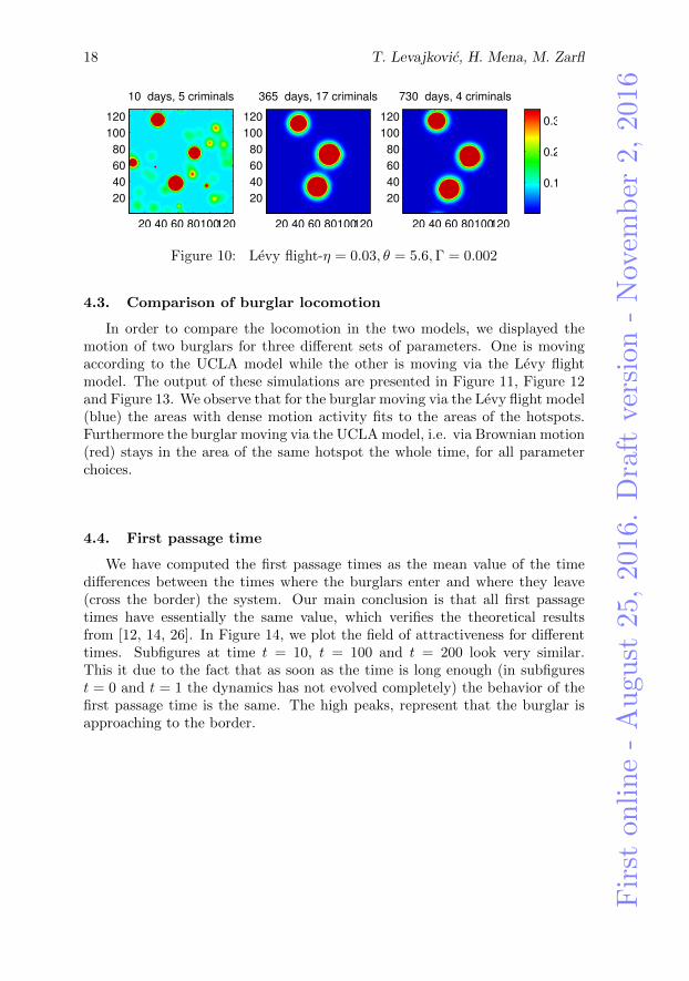
Figure 10: Levy flight-η = 0.03, θ = 5.6,Γ = 0.002
4.3. Comparison of burglar locomotion
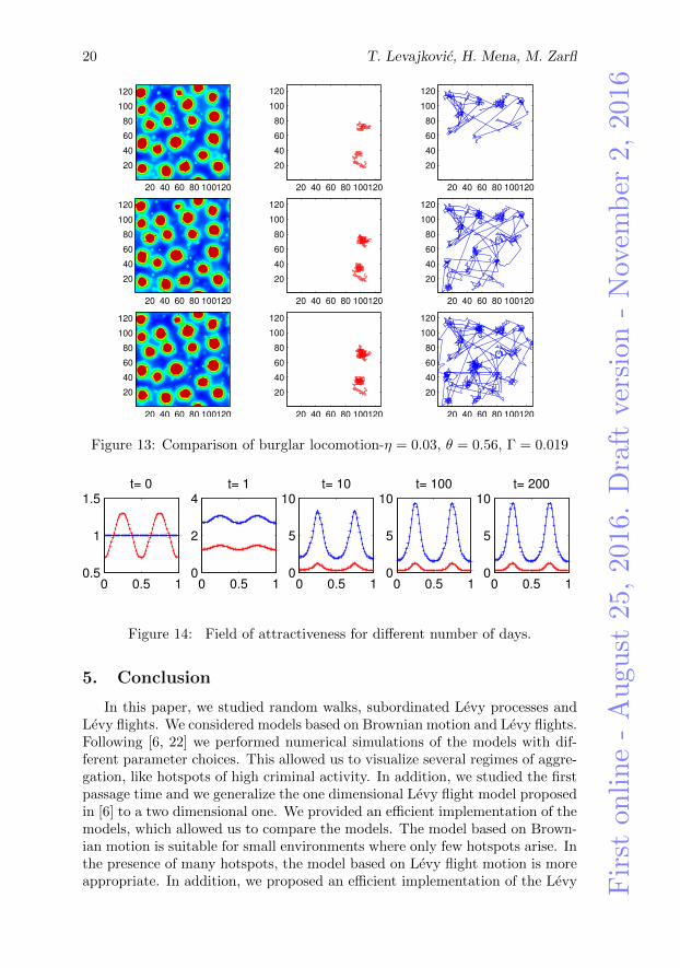
In order to compare the locomotion in the two models, we displayed themotion of two burglars for three different sets of parameters. One is movingaccording to the UCLA model while the other is moving via the Levy flightmodel. The output of these simulations are presented in Figure 11, Figure 12and Figure 13. We observe that for the burglar moving via the Levy flight model(blue) the areas with dense motion activity fits to the areas of the hotspots.Furthermore the burglar moving via the UCLA model, i.e. via Brownian motion(red) stays in the area of the same hotspot the whole time, for all parameterchoices.
4.4. First passage time
We have computed the first passage times as the mean value of the timedifferences between the times where the burglars enter and where they leave(cross the border) the system. Our main conclusion is that all first passagetimes have essentially the same value, which verifies the theoretical resultsfrom [12, 14, 26]. In Figure 14, we plot the field of attractiveness for differenttimes. Subfigures at time t = 10, t = 100 and t = 200 look very similar.This it due to the fact that as soon as the time is long enough (in subfigurest = 0 and t = 1 the dynamics has not evolved completely) the behavior of thefirst passage time is the same. The high peaks, represent that the burglar isapproaching to the border.

Fir
ston
lin
e-
Au
gu
st25
,20
16.
Dra
ftve
rsio
n-
Nov
emb
er2,
2016
Levy processes, subordinators and crime modelling 19
20 40 60 80 100120
20
40
60
80
100
120
20 40 60 80 100120
20
40
60
80
100
120
20 40 60 80 100120
20
40
60
80
100
120
20 40 60 80 100120
20
40
60
80
100
120
20 40 60 80 100120
20
40
60
80
100
120
20 40 60 80 100120
20
40
60
80
100
120
20 40 60 80 100120
20
40
60
80
100
120
20 40 60 80 100120
20
40
60
80
100
120
20 40 60 80 100120
20
40
60
80
100
120
Figure 11: Comparison of burglar locomotion-η = 0.1, θ = 8, Γ = 0.004
20 40 60 80 100120
20
40
60
80
100
120
20 40 60 80 100120
20
40
60
80
100
120
20 40 60 80 100120
20
40
60
80
100
120
20 40 60 80 100120
20
40
60
80
100
120
20 40 60 80 100120
20
40
60
80
100
120
20 40 60 80 100120
20
40
60
80
100
120
20 40 60 80 100120
20
40
60
80
100
120
20 40 60 80 100120
20
40
60
80
100
120
20 40 60 80 100120
20
40
60
80
100
120
Figure 12: Comparison of burglar locomotion-η = 0.1, θ = 10, Γ = 0.0005
Fir
ston
lin
e-
Au
gust
25,
2016.
Dra
ftve
rsio
n-
Nov
emb
er2,
2016
20 T. Levajkovic, H. Mena, M. Zarfl
20 40 60 80 100120
20
40
60
80
100
120
20 40 60 80 100120
20
40
60
80
100
120
20 40 60 80 100120
20
40
60
80
100
120
20 40 60 80 100120
20
40
60
80
100
120
20 40 60 80 100120
20
40
60
80
100
120
20 40 60 80 100120
20
40
60
80
100
120
20 40 60 80 100120
20
40
60
80
100
120
20 40 60 80 100120
20
40
60
80
100
120
20 40 60 80 100120
20
40
60
80
100
120
Figure 13: Comparison of burglar locomotion-η = 0.03, θ = 0.56, Γ = 0.019
0 0.5 10.5
1
1.5
t= 0
0 0.5 10
2
4
t= 1
0 0.5 10
5
10
t= 10
0 0.5 10
5
10
t= 100
0 0.5 10
5
10
t= 200
Figure 14: Field of attractiveness for different number of days.
5. Conclusion
In this paper, we studied random walks, subordinated Levy processes andLevy flights. We considered models based on Brownian motion and Levy flights.Following [6, 22] we performed numerical simulations of the models with dif-ferent parameter choices. This allowed us to visualize several regimes of aggre-gation, like hotspots of high criminal activity. In addition, we studied the firstpassage time and we generalize the one dimensional Levy flight model proposedin [6] to a two dimensional one. We provided an efficient implementation of themodels, which allowed us to compare the models. The model based on Brown-ian motion is suitable for small environments where only few hotspots arise. Inthe presence of many hotspots, the model based on Levy flight motion is moreappropriate. In addition, we proposed an efficient implementation of the Levy

Fir
stonline
-A
ugust
25,
2016.
Dra
ftver
sion
-N
ovem
ber
2,
2016
Levy processes, subordinators and crime modelling 21
model by using high performance computing techniques. This allowed us toperform numerical simulations with the Levy model at the computational costof the Brownian motion based model, making feasible for real life applications.
Acknowledgement
The paper was supported by the project Numerical methods in Simula-tion and Optimal Control through the program Nachwuchsforderung 2014 atUniversity of Innsbruck.
References
[1] Applebaum, D., Levy processes and stochastic calculus. 2nd edition, Cambridgestudies in advanced mathematics 116, Cambridge University Press, 2009.
[2] Benner, P., Ezzatti, P., Mena, H., Quintana-Ort, E.S., Remon, A., Solvingmatrix equations on multi-core and many-core architectures. Algorithms 6 (4)(2013), 857–870.
[3] Benner, P., Mena H., Numerical solution of the infinite-dimensional LQR-problem and the associated Riccati differential equations. J. Numer. Math., DeGruyter just accepted, (2016), DOI: 10.1515/jnma-2016-1039.
[4] Benner, P., Mena H., Rosenbrock methods for solving differential Riccati equa-tions. IEEE Trans. Automat. Control 58 (11) (2013), 2950–2957.
[5] Bogachev, L. V., Random walks in random environments. In: Encyclopediao Mathematical Physics 4, (J.-P. Francoise et al. eds.), pp. 353–371, Oxford:Elsevier, 2006.
[6] Chaturapruek, S., Breslau, J., Yazdi, D., Kolokolnikov, T., McCalla, S. G.,Crime modelling with Levy flights. SIAM J. Appl. Math. 73 (4) (2013), 1703–1720.
[7] Chechkin, A. V., Metzler, R., Klafter, J., Gonchar, V. Yu., Introduction to thetheory of Levy flights. In: Anomalous Transport: Foundations and Applications,(R. Klages et al. eds.), pp. 129–162. Wiley-VCH Verlag GmbH & Co. KGaA,2008.
[8] Feller, W., An introduction to probability theory and its applications. Vol. I,3rd edition, New York - London - Sydney: John Wiley & Sons, Inc., 1968.
[9] Geman, H., Madan, D., Yor, M., Asset prices are Brownian motion: only inbusiness time. Quantitative Analysis in Financial Markets, River Edge, NY:World Sci. Publ., (2001), 103–146.
[10] Hilber, N., Reichmann, O., Schwab, C., Winter, C., Computational methods forquantitative finance: Finite element methods for derivative pricing. Heidelberg:Springer, 2013.
[11] Huang, Y., Oberman, A., Numerical methods for fractional Laplacian: a finitedifference-quadrature approach. SIAM J. Numer. Anal. 52 (2014), 3056–3084.
[12] Hurd, T. R., Kuznetsov, A., On the first passage time for Brownian motionsubordinated by a Levy process. J. Appl. Probab. 46 (1) (2009), 181–198.

Fir
ston
lin
e-
Au
gust
25,
2016.
Dra
ftve
rsio
n-
Nov
emb
er2,
2016
22 T. Levajkovic, H. Mena, M. Zarfl
[13] Hughes, B. D., Random walks and random environments. Volume 1: Randomwalks, Oxford Science Publications. New York: The Clarendon Press, OxfordUniversity Press, 1995.
[14] Karatzas, I., Shreve, S. E., Brownian motion and stochastic calculus. GraduateTexts in Mathematics 113, 2nd edition, New York: Springer-Verlag, 1991.
[15] Kyprianou, A. E., Introductory lectures on fluctuations of Levy processes withapplications. Universitext. Berlin: Springer-Verlag, 2006.
[16] Lang, N., Mena, H., Saak, J., On the benefits of the LDL factorization forlarge-scale differential matrix equation solvers. Linear Algebra Appl. 480 (2015),44–71.
[17] Metzler, R., Klafter, J., The random walks guide to anomalous diffusion: Afractional dynamic approach. Phys. Rep. 339 (1) (2000), 1–77.
[18] Revuz, D., Yor, M., Continuous martingales and Brownian motion. FundamentalPrinciples of Mathematical Sciences 293, 3rd edition, Berlin: Springer-Verlag,1999.
[19] Rey, S. J., Mack, E. A., Koschinsky, J., Exploratory space-time analysis ofburglary patterns. J. Quant. Criminol. 28 (3) (2012), 509–531.
[20] Samorodnitsky, G., Taqqu, M., Stable non-Gaussian random processes. Stochas-tic models with infinite variance. Stochastic Modeling. New York: Chapman &Hall, 1994.
[21] Sato, K., Levy processes and infinitely divisible distributions. Cambridge Studiesin Advanced Mathematics 68, Cambridge: Cambridge University Press, 2013.
[22] Short, M. B., D’Orsogna, M. R., Pasour, V. B., Tita, G. E., Brantingham, P. J.,Bertozzi, A. L., Chayes, L. B., A statistical model of criminal behavior. Math.Models Methods Appl. Sci. 18 (2008), 1249–1267.
[23] Sims, D. W., Humphries, N. E., Bradford, R. W., Bruce, B. D., Levy flight andBrownian search patterns of a free-ranging predator reflect different prey field.J Anim Ecol. 81 (2) (2012), 432–442.
[24] Sokolov, I. M., Levy flights from continuous-time process. Phys. Rev. E 63(011104) (2000), 1–10.
[25] Song, R., Vondracek, Z., Potential theory of special subordinators and subordi-nate killed stable processes. J. Theoret. Probab. 19 (4) (2006), 817–847.
[26] Taqqu, M., Veillette, M., Numerical computation of first-passage times of in-creasing Levy processes. Methodol. Comput. Appl. Probab. 12 (4) (2010), 695–729.
[27] Van Koppen, P. J., Jansen, R. W. J., The road to the robbery: Travel patternsin commercial robberies. Br. J. Criminol. 38 (2) (1998), 230–246.
[28] Warren, J., Yor, M., The Brownian burglar: conditioning Brownian motion byits local time process. Seminare de Probabilites, XXXII, pp. 328–342, LectureNotes in Math. 1686, Berlin: Springer, 1998.
[29] Zipkin, J. R., Short, M. B., Bertozzi A. L., Cops on the dots in a mathematicalmodel of urban crime and police response. Discrete Contin. Dyn. Syst. Ser. B19 (5) (2014), 1479–1506.

Fir
ston
lin
e-
Au
gu
st25
,20
16.
Dra
ftve
rsio
n-
Nov
emb
er2,
2016
Levy processes, subordinators and crime modelling 23
Received by the editors February 5, 2016First published online August 25, 2016