Novel Geometry Design for Intensified CO2 AbsorbersGrigorios Panagakos, Research EngineerCarnegie Mellon University-LRST National Energy Technology Laboratory

2

Highlights

Computationally generated TPMS structures on CAD files

CFD models capturing fluid dynamics forcountercurrent gas/solvent flow in TPMS geometries

Model validation using random rings packing

Results on hydrodynamics of TPMS geometries Blockage of flow Effects of viscosity and liquid flowrate oninterfacial and wetted area

Reactive systems for CO2 absorption on CFD models

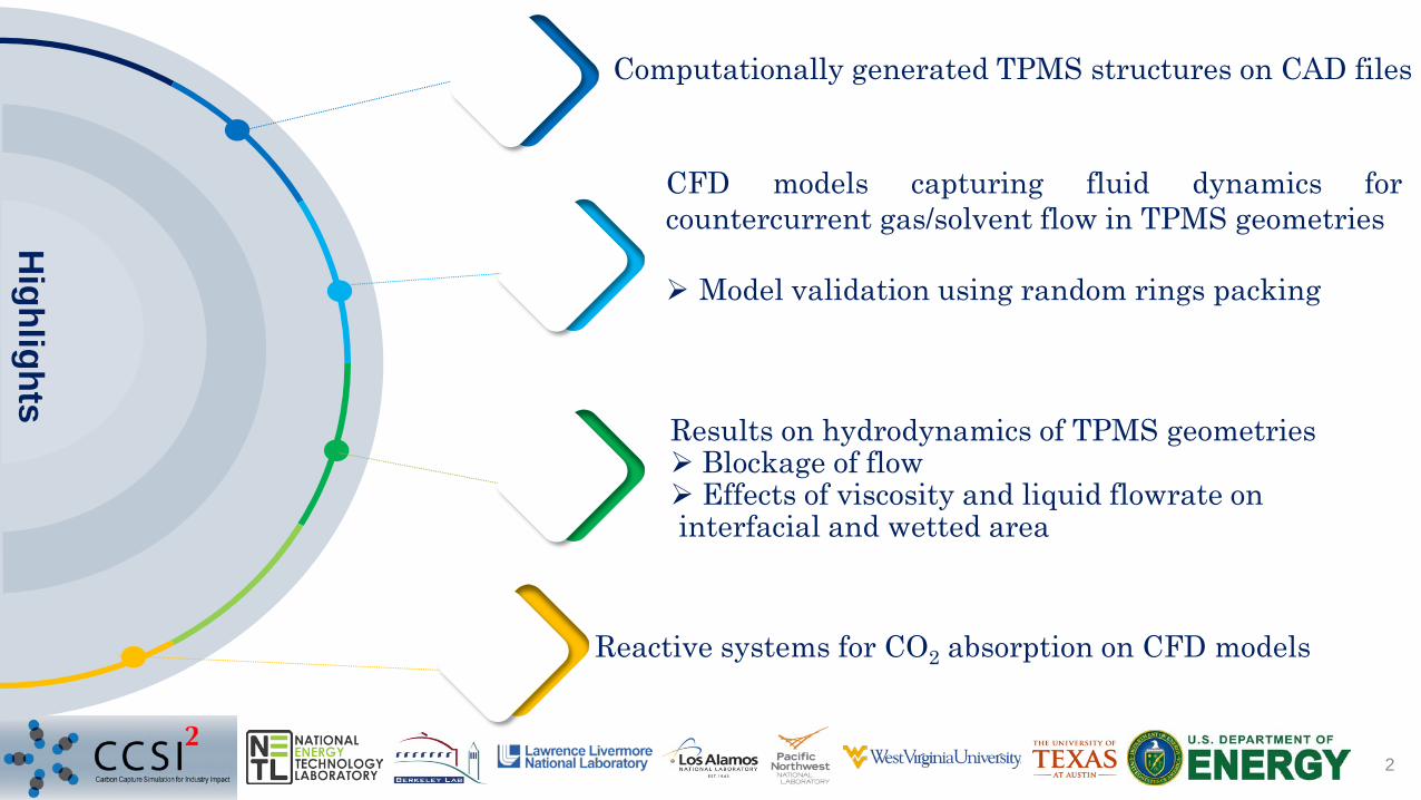
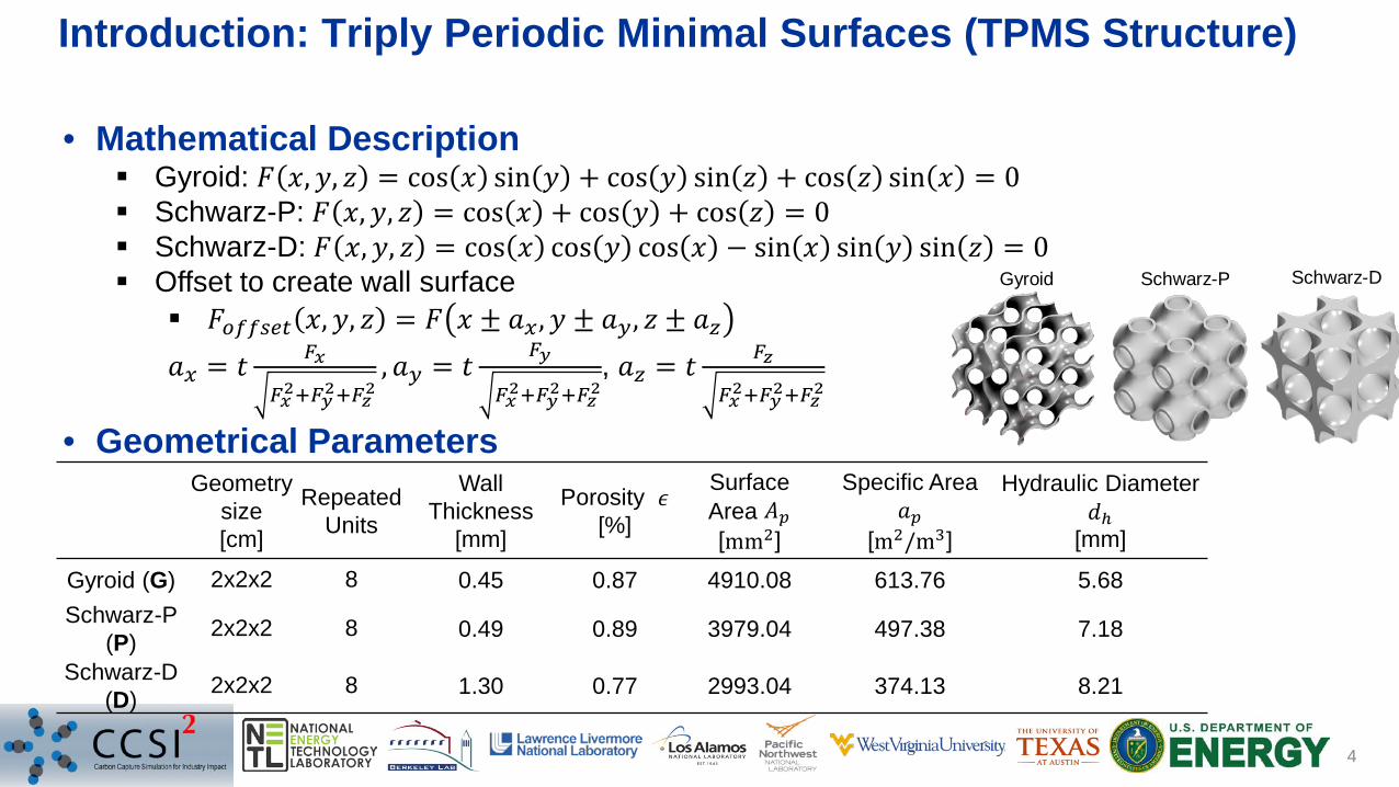
Introduction: Triply Periodic Minimal Surfaces (TPMS Structure)

3

• Advantages of TPMS Improved heat transfer (~10X) Separate independent flow

channels

• For carbon capture• Mass transfer

coefficients?• Mass transfer areas?• Highly viscous solvent?

• Objective: CFD modeling for the gas/solvent flow in TPMS

Gyroid Schwarz-P Schwarz-D

3D printed Gyroid@ LLNL

Introduction: Triply Periodic Minimal Surfaces (TPMS Structure)

4

• Mathematical Description Gyroid: 𝐹𝐹 𝑥𝑥,𝑦𝑦, 𝑧𝑧 = cos 𝑥𝑥 sin 𝑦𝑦 + cos 𝑦𝑦 sin 𝑧𝑧 + cos 𝑧𝑧 sin 𝑥𝑥 = 0 Schwarz-P: 𝐹𝐹 𝑥𝑥,𝑦𝑦, 𝑧𝑧 = cos 𝑥𝑥 + cos 𝑦𝑦 + cos 𝑧𝑧 = 0 Schwarz-D: 𝐹𝐹 𝑥𝑥,𝑦𝑦, 𝑧𝑧 = cos 𝑥𝑥 cos 𝑦𝑦 cos 𝑥𝑥 − sin 𝑥𝑥 sin 𝑦𝑦 sin 𝑧𝑧 = 0 Offset to create wall surface

𝐹𝐹𝑜𝑜𝑜𝑜𝑜𝑜𝑜𝑜𝑜𝑜𝑜𝑜 𝑥𝑥,𝑦𝑦, 𝑧𝑧 = 𝐹𝐹 𝑥𝑥 ± 𝑎𝑎𝑥𝑥,𝑦𝑦 ± 𝑎𝑎𝑦𝑦, 𝑧𝑧 ± 𝑎𝑎𝑧𝑧𝑎𝑎𝑥𝑥 = 𝑡𝑡 𝐹𝐹𝑥𝑥

𝐹𝐹𝑥𝑥2+𝐹𝐹𝑦𝑦2+𝐹𝐹𝑧𝑧2,𝑎𝑎𝑦𝑦 = 𝑡𝑡 𝐹𝐹𝑦𝑦

𝐹𝐹𝑥𝑥2+𝐹𝐹𝑦𝑦2+𝐹𝐹𝑧𝑧2, 𝑎𝑎𝑧𝑧 = 𝑡𝑡 𝐹𝐹𝑧𝑧

𝐹𝐹𝑥𝑥2+𝐹𝐹𝑦𝑦2+𝐹𝐹𝑧𝑧2

• Geometrical Parameters

Gyroid Schwarz-P Schwarz-D

Geometry size[cm]

RepeatedUnits

Wall Thickness

[mm]

Porosity 𝜖𝜖[%]

SurfaceArea 𝐴𝐴𝑝𝑝[mm2]

Specific Area 𝑎𝑎𝑝𝑝

[m2/m3]

Hydraulic Diameter 𝑑𝑑ℎ

[mm]

Gyroid (G) 2x2x2 8 0.45 0.87 4910.08 613.76 5.68Schwarz-P

(P) 2x2x2 8 0.49 0.89 3979.04 497.38 7.18

Schwarz-D (D) 2x2x2 8 1.30 0.77 2993.04 374.13 8.21

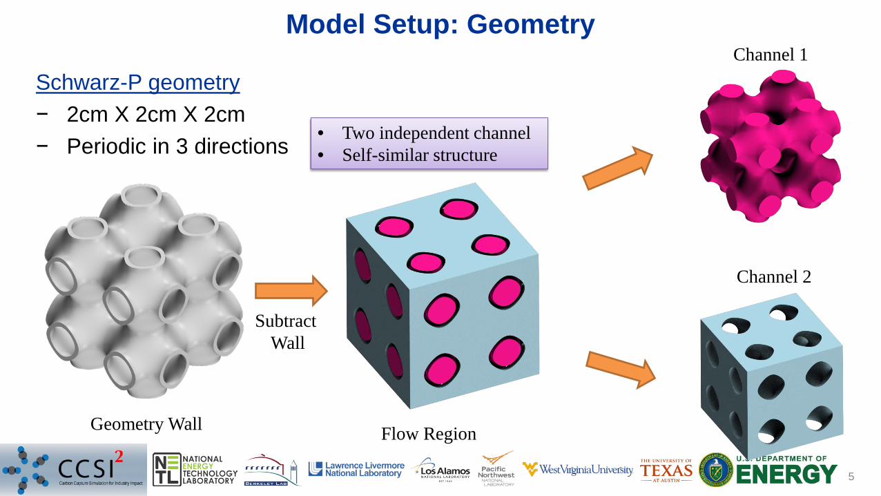
Model Setup: Geometry

5

Schwarz-P geometry− 2cm X 2cm X 2cm− Periodic in 3 directions

Geometry Wall

Channel 2

Channel 1

• Two independent channel • Self-similar structure

Flow Region

SubtractWall

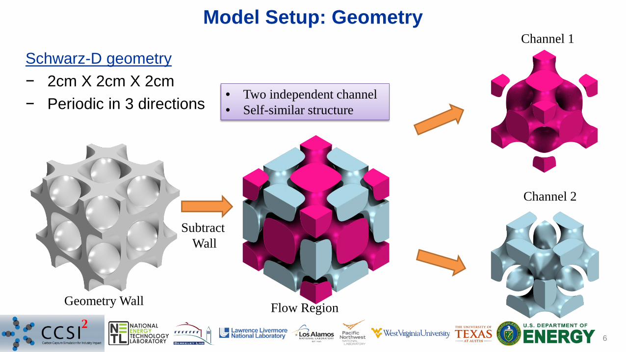
Model Setup: Geometry

6

Schwarz-D geometry− 2cm X 2cm X 2cm− Periodic in 3 directions

Geometry Wall

Channel 2

Channel 1

• Two independent channel • Self-similar structure

Flow Region

SubtractWall

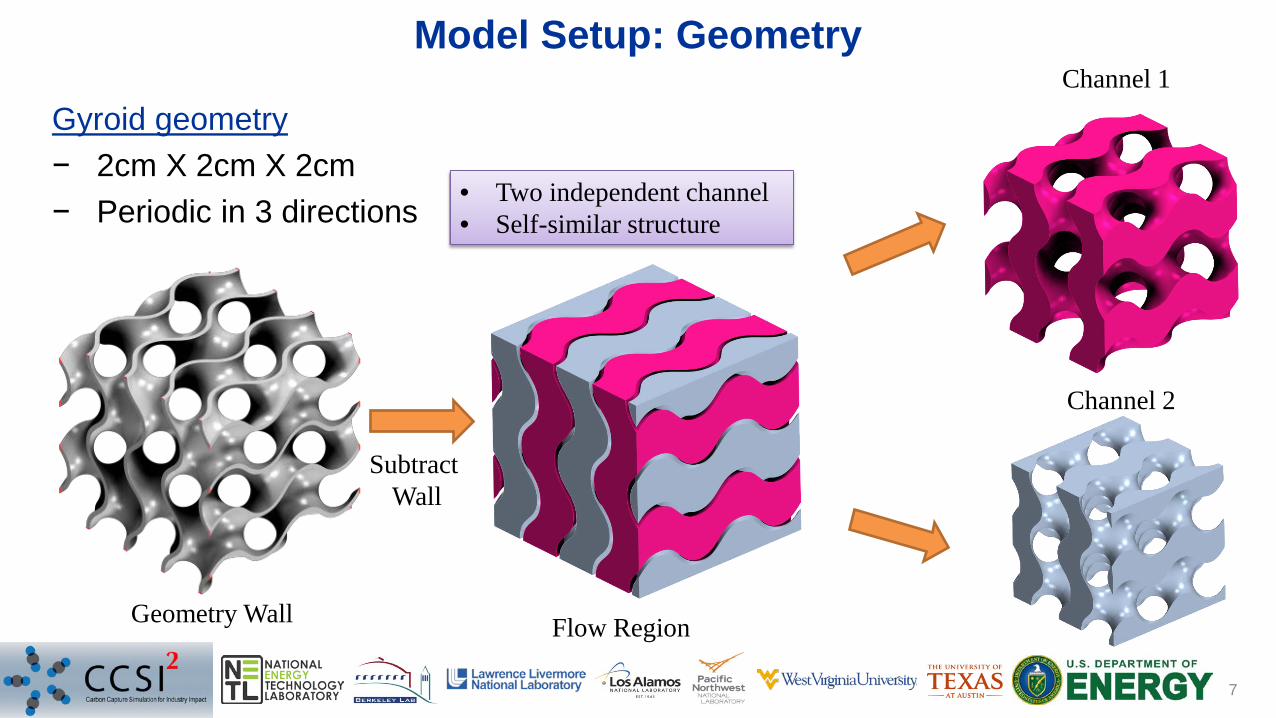
Model Setup: Geometry

7

Gyroid geometry− 2cm X 2cm X 2cm− Periodic in 3 directions

Geometry Wall

Channel 2

Channel 1

• Two independent channel • Self-similar structure

Flow Region

SubtractWall

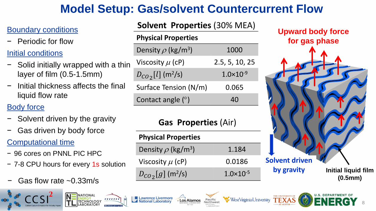
Model Setup: Gas/solvent Countercurrent Flow

8

Boundary conditions− Periodic for flowInitial conditions− Solid initially wrapped with a thin

layer of film (0.5-1.5mm)− Initial thickness affects the final

liquid flow rateBody force− Solvent driven by the gravity− Gas driven by body force Computational time− 96 cores on PNNL PIC HPC− 7-8 CPU hours for every 1s solution

Initial liquid film (0.5mm)

Upward body force for gas phasePhysical Properties

Density ρ (kg/m3) 1000Viscosity µ (cP) 2.5, 5, 10, 25𝐷𝐷𝐶𝐶𝐶𝐶2[𝑙𝑙] (m2/s) 1.0×10-9

Surface Tension (N/m) 0.065Contact angle (°) 40

Solvent Properties (30% MEA)

Physical PropertiesDensity ρ (kg/m3) 1.184Viscosity µ (cP) 0.0186𝐷𝐷𝐶𝐶𝐶𝐶2[𝑔𝑔] (m2/s) 1.0×10-5

Gas Properties (Air)

− Gas flow rate ~0.33m/s

Solvent driven by gravity

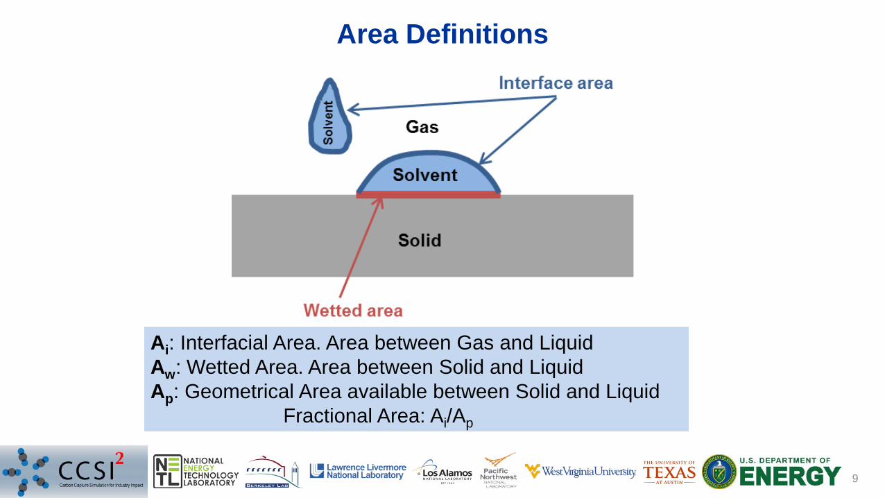
Area Definitions

9

Ai: Interfacial Area. Area between Gas and LiquidAw: Wetted Area. Area between Solid and LiquidAp: Geometrical Area available between Solid and Liquid

Fractional Area: Ai/Ap

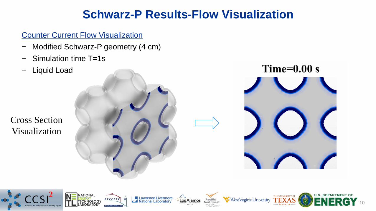
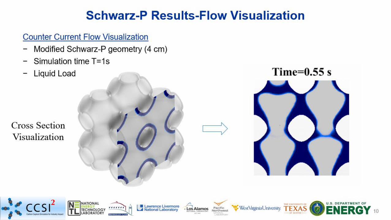
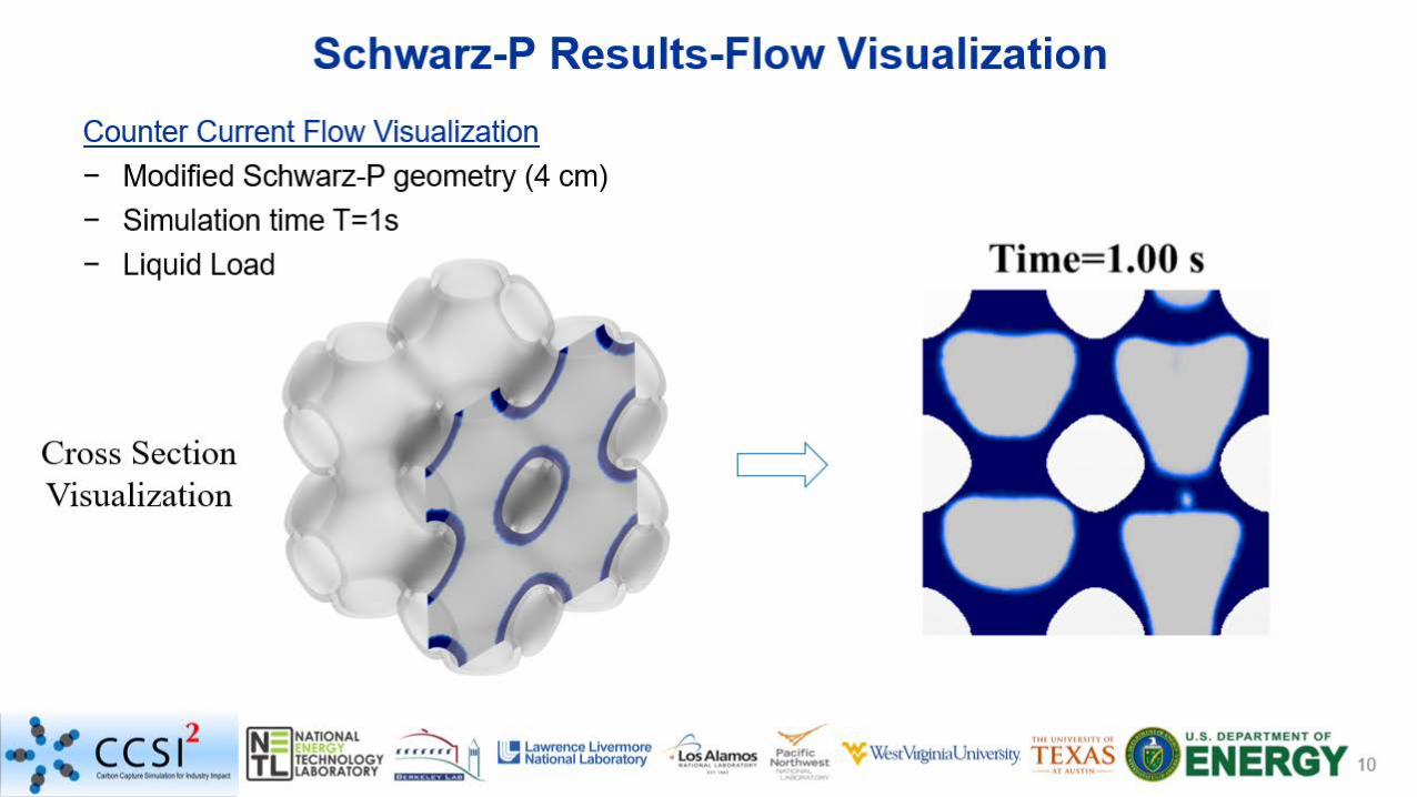
Schwarz-P Results-Flow Visualization

10

Cross Section Visualization

Counter Current Flow Visualization− Modified Schwarz-P geometry (4 cm)− Simulation time T=1s− Liquid Load

11

12

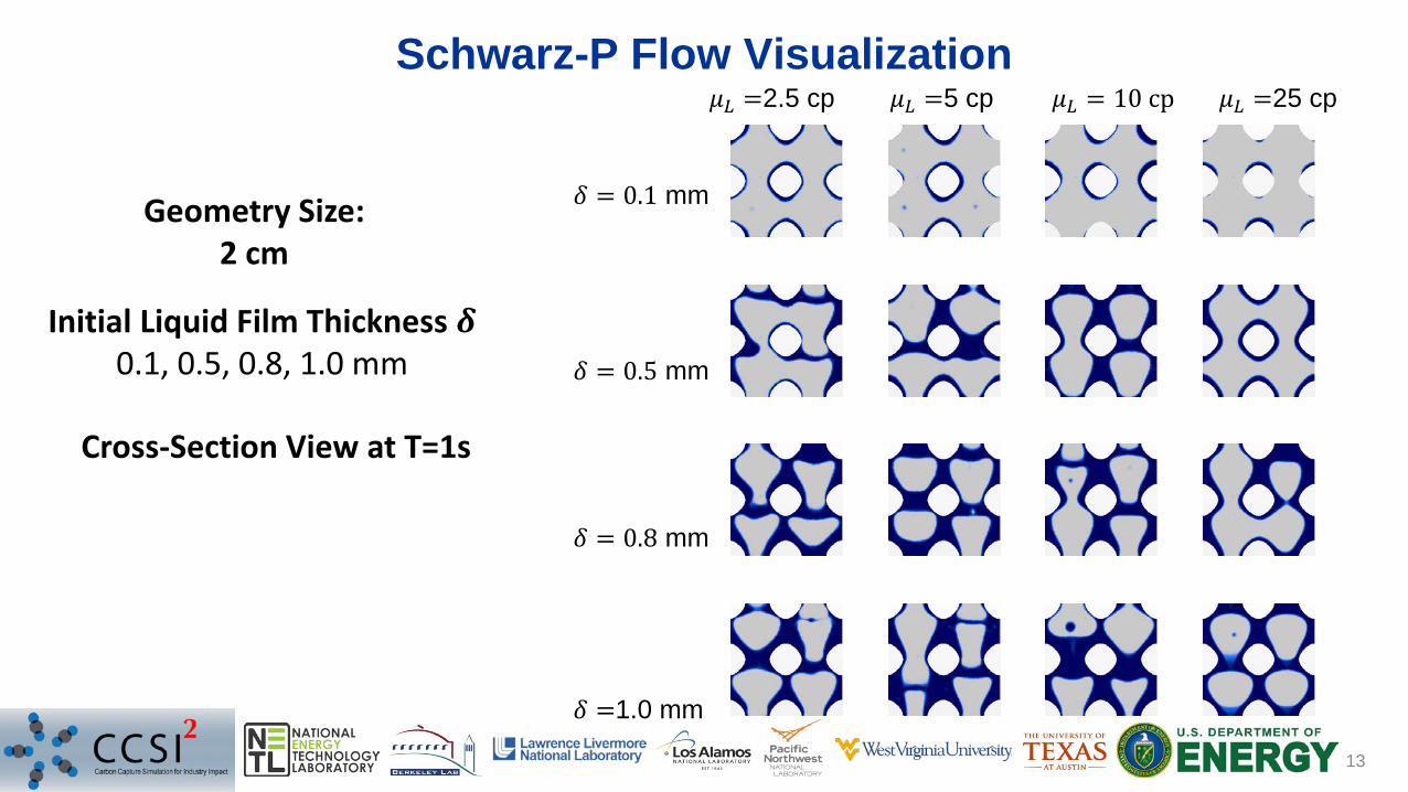
Schwarz-P Flow Visualization

13

𝜇𝜇𝐿𝐿 =2.5 cp 𝜇𝜇𝐿𝐿 =5 cp 𝜇𝜇𝐿𝐿 = 10 cp 𝜇𝜇𝐿𝐿 =25 cp

𝛿𝛿 = 0.1 mm

𝛿𝛿 = 0.5 mm

𝛿𝛿 = 0.8 mm

𝛿𝛿 =1.0 mm

Initial Liquid Film Thickness 𝜹𝜹0.1, 0.5, 0.8, 1.0 mm

Geometry Size: 2 cm

Cross-Section View at T=1s

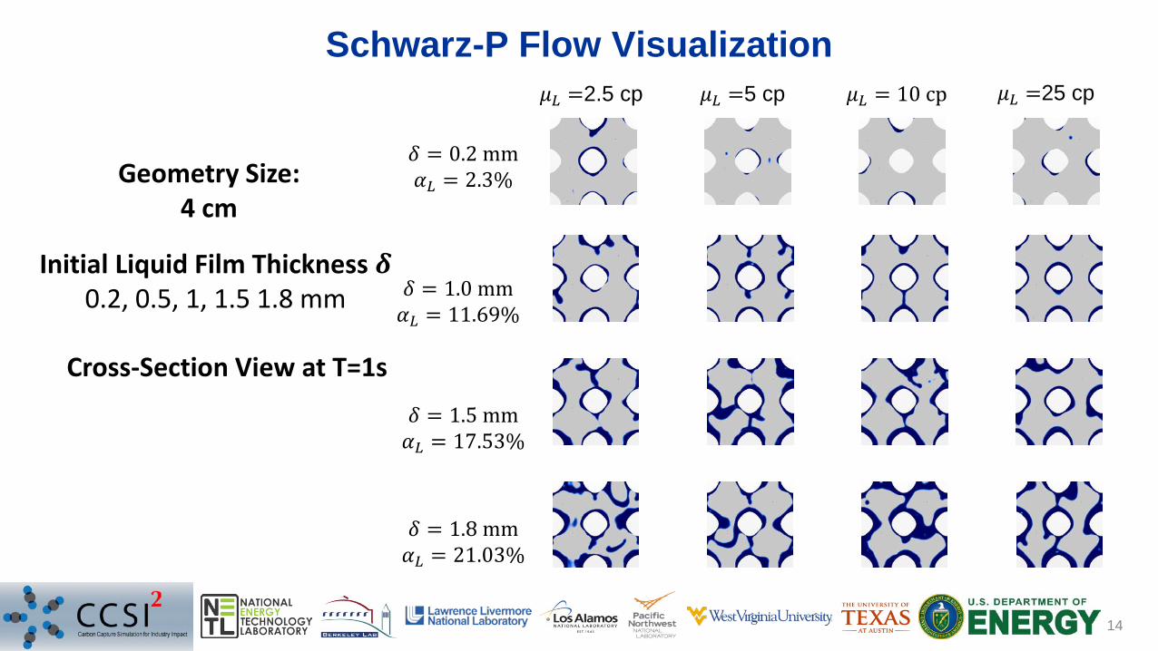
Schwarz-P Flow Visualization

14

Initial Liquid Film Thickness 𝜹𝜹0.2, 0.5, 1, 1.5 1.8 mm

Geometry Size: 4 cm

𝛿𝛿 = 0.2 mm𝛼𝛼𝐿𝐿 = 2.3%

𝛿𝛿 = 1.0 mm𝛼𝛼𝐿𝐿 = 11.69%

𝛿𝛿 = 1.5 mm𝛼𝛼𝐿𝐿 = 17.53%

𝛿𝛿 = 1.8 mm𝛼𝛼𝐿𝐿 = 21.03%

𝜇𝜇𝐿𝐿 =2.5 cp 𝜇𝜇𝐿𝐿 =5 cp 𝜇𝜇𝐿𝐿 = 10 cp 𝜇𝜇𝐿𝐿 =25 cp

Cross-Section View at T=1s

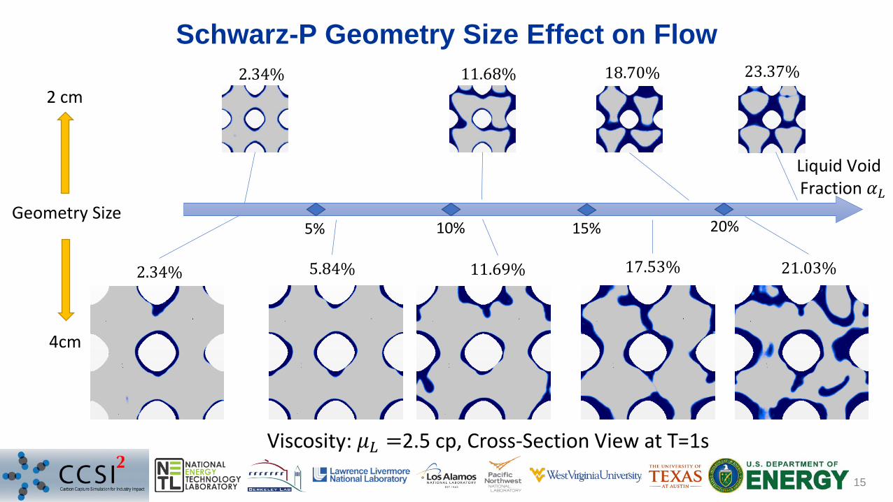
Schwarz-P Geometry Size Effect on Flow

15

Liquid VoidFraction 𝛼𝛼𝐿𝐿

5% 10% 15% 20%

2.34% 5.84% 11.69% 21.03%17.53%

2.34% 11.68% 18.70% 23.37%

Viscosity: 𝜇𝜇𝐿𝐿 =2.5 cp, Cross-Section View at T=1s

Geometry Size

2 cm

4cm

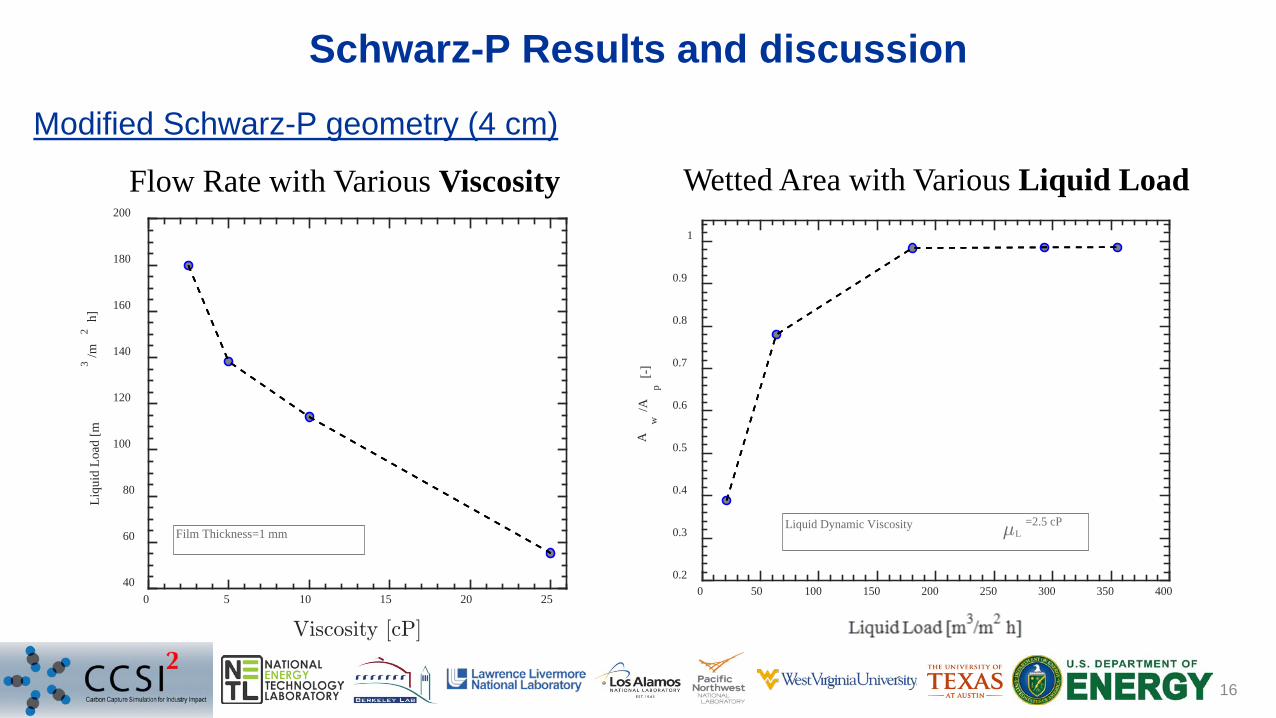
Schwarz-P Results and discussion

16

Modified Schwarz-P geometry (4 cm)

0 5 10 15 20 2540

60

80

100

120

140

160

180

200

Liqu

id L

oad

[m3

/m2

h]

Film Thickness=1 mm

Flow Rate with Various Viscosity Wetted Area with Various Liquid Load

0 50 100 150 200 250 300 350 400

Liquid Load [m3 /m

2 h]

0.2

0.3

0.4

0.5

0.6

0.7

0.8

0.9

1

Aw

/Ap

[-]

Liquid Dynamic Viscosity L

=2.5 cP

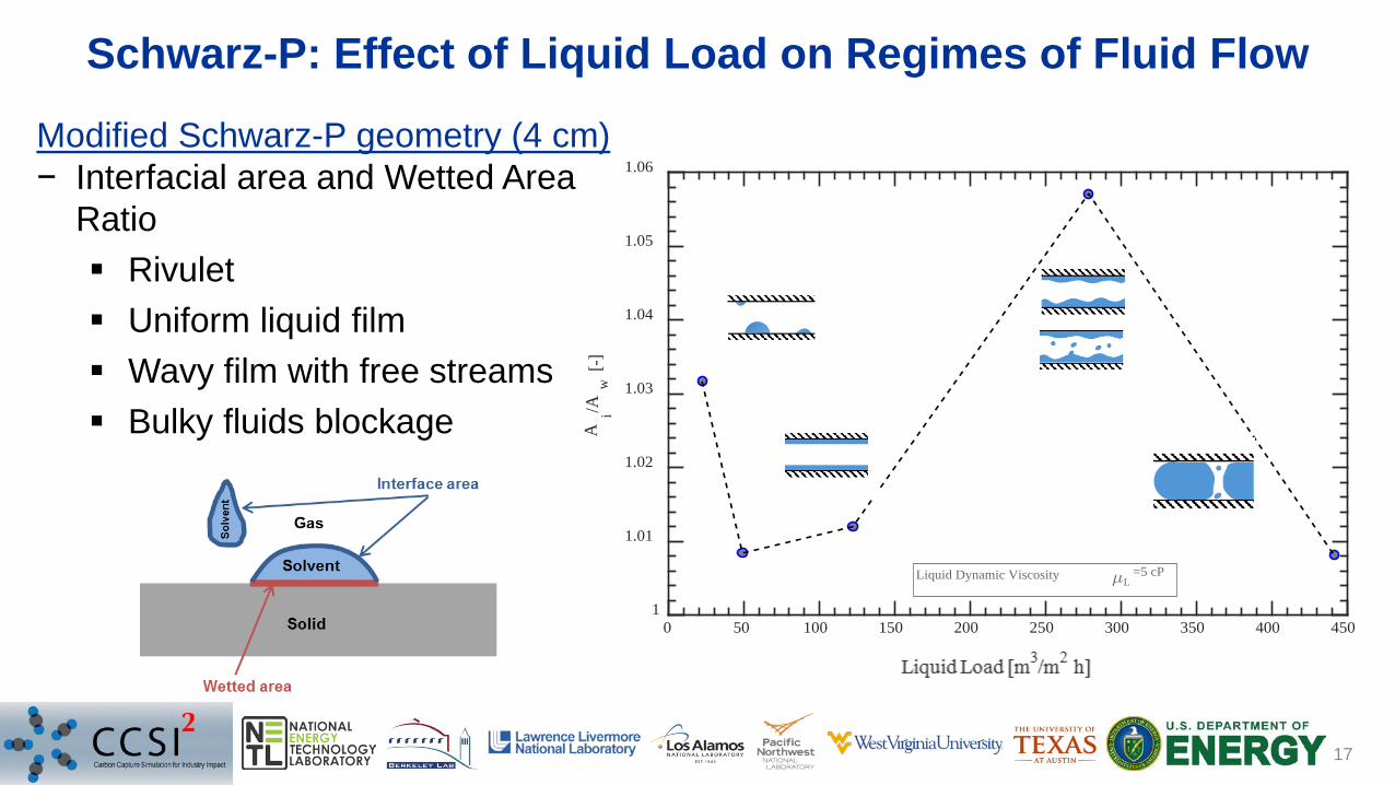
Schwarz-P: Effect of Liquid Load on Regimes of Fluid Flow

17

Modified Schwarz-P geometry (4 cm)− Interfacial area and Wetted Area

Ratio Rivulet Uniform liquid film Wavy film with free streams Bulky fluids blockage

0 50 100 150 200 250 300 350 400 450

Liquid Load [m3 /m 2 h]

1

1.01

1.02

1.03

1.04

1.05

1.06

Ai/A

w [-

]Liquid Dynamic Viscosity L

=5 cP

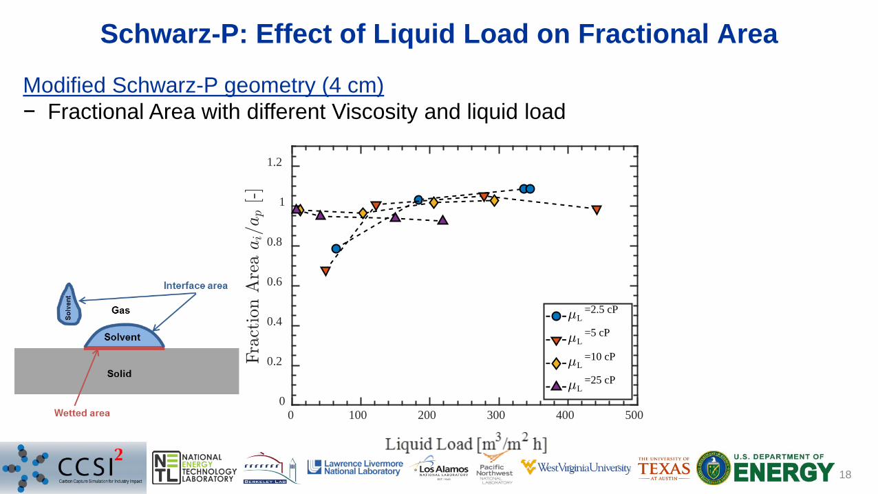
Schwarz-P: Effect of Liquid Load on Fractional Area

18

Modified Schwarz-P geometry (4 cm)− Fractional Area with different Viscosity and liquid load

0 100 200 300 400 500

Liquid Load [m3 /m 2 h]

0

0.2

0.4

0.6

0.8

1

1.2

L=2.5 cP

L=5 cP

L=10 cP

L=25 cP

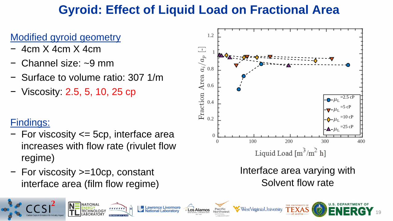
Gyroid: Effect of Liquid Load on Fractional Area

19

Modified gyroid geometry − 4cm X 4cm X 4cm − Channel size: ~9 mm− Surface to volume ratio: 307 1/m− Viscosity: 2.5, 5, 10, 25 cp

Findings:− For viscosity <= 5cp, interface area

increases with flow rate (rivulet flow regime)

− For viscosity >=10cp, constant interface area (film flow regime)

Interface area varying with Solvent flow rate

0 100 200 300 400

Liquid Load [m3 /m 2 h]

0

0.2

0.4

0.6

0.8

1

1.2

L=2.5 cP

L=5 cP

L=10 cP

L=25 cP

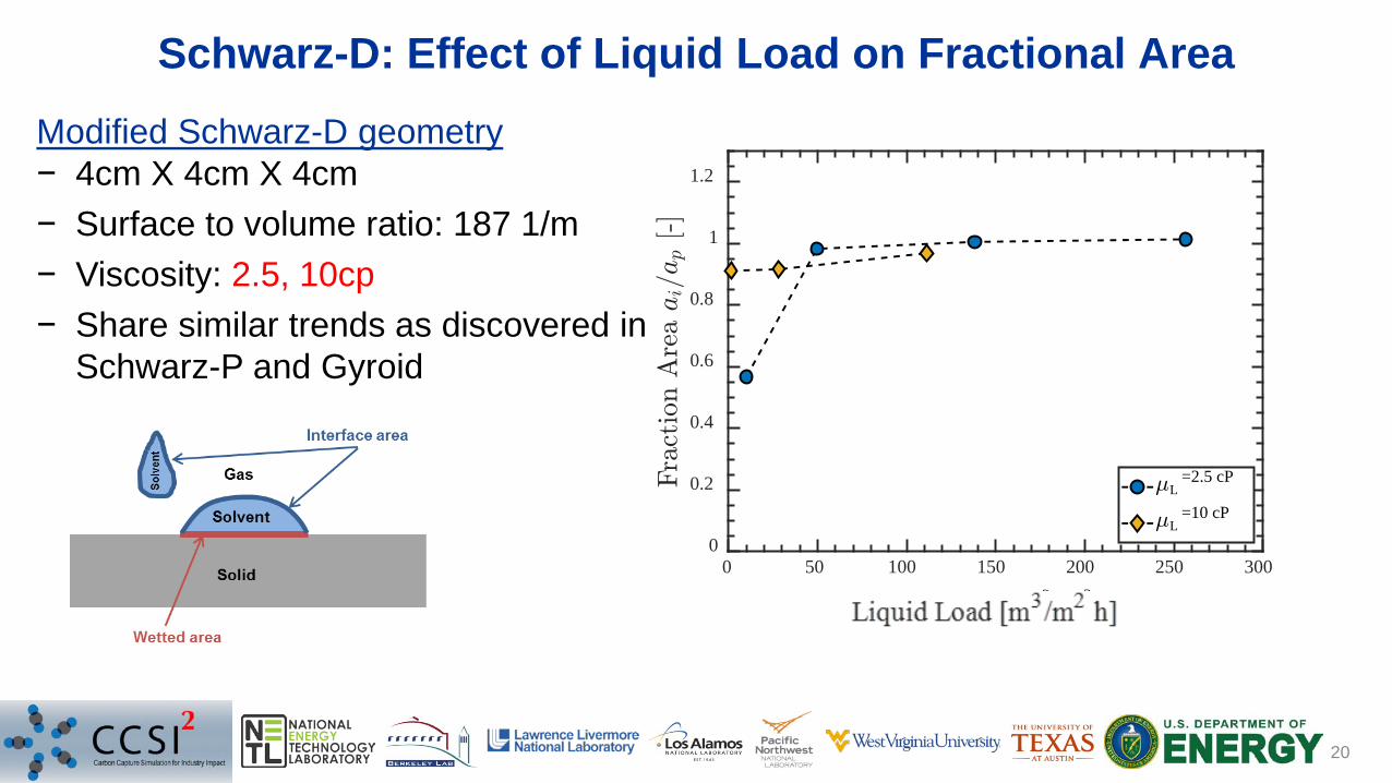
Schwarz-D: Effect of Liquid Load on Fractional Area

20

0 50 100 150 200 250 300

Liquid Load [m3 /m 2 h]

0

0.2

0.4

0.6

0.8

1

1.2

L=2.5 cP

L=10 cP

Modified Schwarz-D geometry − 4cm X 4cm X 4cm − Surface to volume ratio: 187 1/m− Viscosity: 2.5, 10cp− Share similar trends as discovered in

Schwarz-P and Gyroid

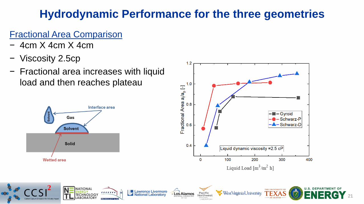
Hydrodynamic Performance for the three geometries

21

Fractional Area Comparison− 4cm X 4cm X 4cm − Viscosity 2.5cp− Fractional area increases with liquid

load and then reaches plateau

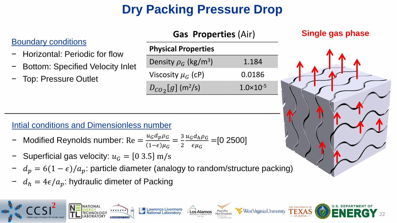
Dry Packing Pressure Drop

22

Boundary conditions− Horizontal: Periodic for flow− Bottom: Specified Velocity Inlet− Top: Pressure Outlet

Single gas phase

Physical PropertiesDensity 𝜌𝜌𝐺𝐺 (kg/m3) 1.184Viscosity 𝜇𝜇𝐺𝐺 (cP) 0.0186𝐷𝐷𝐶𝐶𝐶𝐶2[𝑔𝑔] (m2/s) 1.0×10-5

Gas Properties (Air)

Intial conditions and Dimensionless number

− Modified Reynolds number: Re = 𝑢𝑢𝐺𝐺𝑑𝑑𝑝𝑝𝜌𝜌𝐺𝐺1−𝜖𝜖 𝜇𝜇𝐺𝐺

= 32𝑢𝑢𝐺𝐺𝑑𝑑ℎ𝜌𝜌𝐺𝐺𝜖𝜖𝜇𝜇𝐺𝐺

=[0 2500]

− Superficial gas velocity: 𝑢𝑢𝐺𝐺 = 0 3.5 m/s− 𝑑𝑑𝑝𝑝 = 6(1 − 𝜖𝜖)/𝑎𝑎𝑝𝑝: particle diameter (analogy to random/structure packing)− 𝑑𝑑ℎ = 4𝜖𝜖/𝑎𝑎𝑝𝑝: hydraulic dimeter of Packing

Dry Packing Pressure Drop

23

0.0

1.0

2.0

3.0

4.0

5.0

6.0

7.0

0 500 1000 1500 2000

Res

ista

nce

Coe

ffici

ent ψ

Re

Resistant Coefficient

Schwarz-DSchwarz-PGyroidErgun

0

500

1000

1500

2000

2500

3000

3500

4000

0 500 1000 1500 2000 2500

dp/d

h [P

a/m

]

Re

Pressure Drop

Schwarz-D

Schwarz-P

Gyroid Ergun Equation:𝜓𝜓 = 150

𝑅𝑅𝑜𝑜+ 1.75

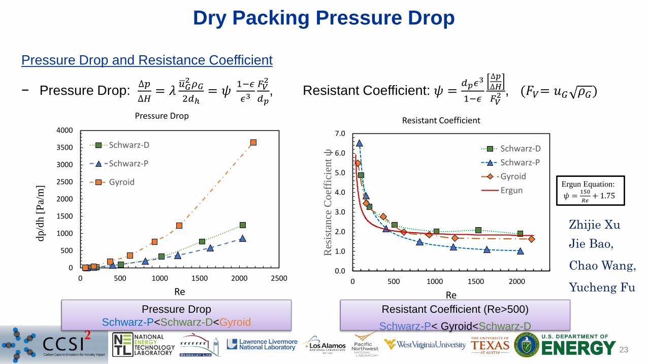
Pressure Drop and Resistance Coefficient

− Pressure Drop: ∆𝑝𝑝∆𝐻𝐻

= 𝜆𝜆 �𝑢𝑢𝐺𝐺2𝜌𝜌𝐺𝐺2𝑑𝑑ℎ

= 𝜓𝜓 1−𝜖𝜖𝜖𝜖3

𝐹𝐹𝑉𝑉2

𝑑𝑑𝑝𝑝, Resistant Coefficient: 𝜓𝜓 = 𝑑𝑑𝑝𝑝𝜖𝜖3

1−𝜖𝜖

∆𝑝𝑝∆𝐻𝐻𝐹𝐹𝑉𝑉2 , (𝐹𝐹𝑉𝑉= 𝑢𝑢𝐺𝐺 𝜌𝜌𝐺𝐺)

Pressure DropSchwarz-P<Schwarz-D<Gyroid

Resistant Coefficient (Re>500)Schwarz-P< Gyroid<Schwarz-D

Zhijie XuJie Bao, Chao Wang, Yucheng Fu

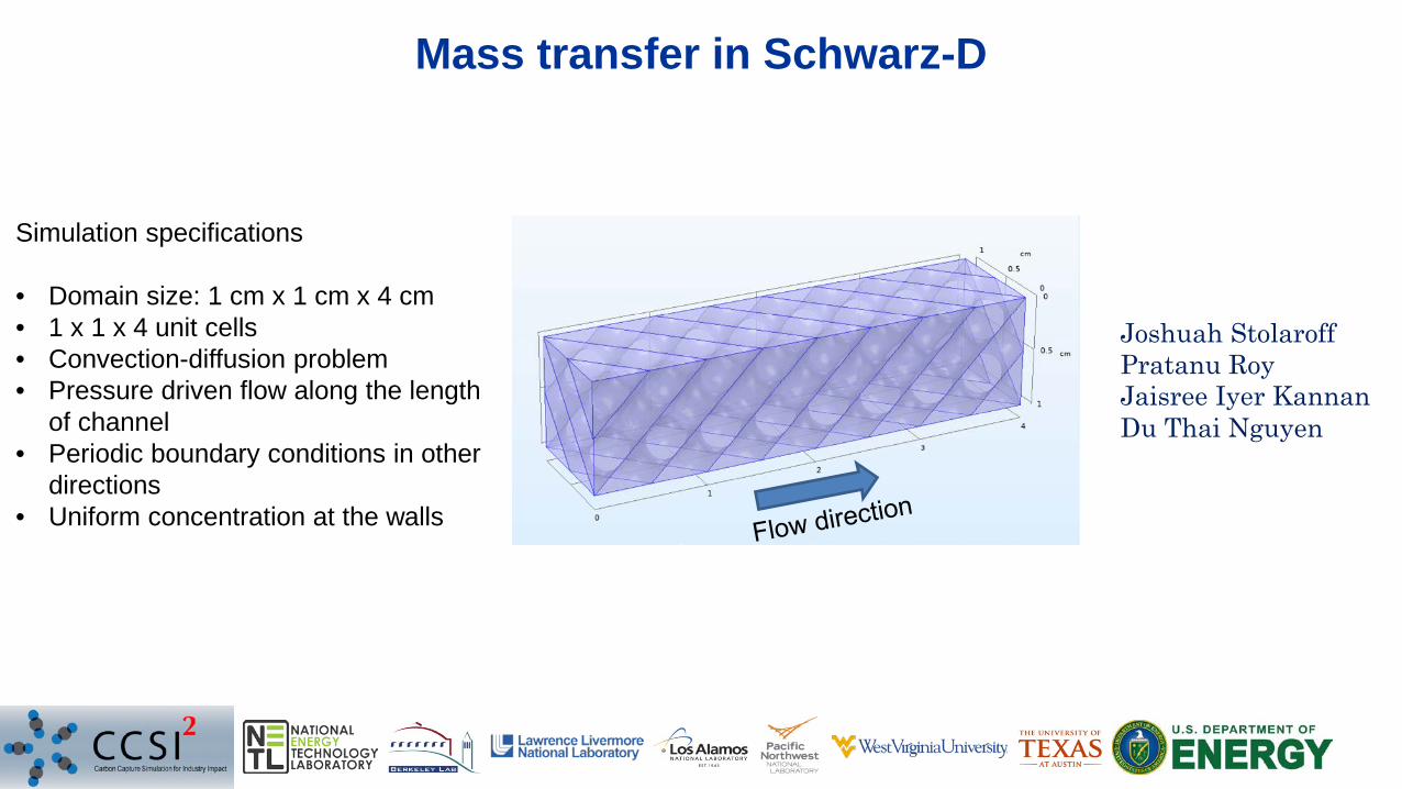
Mass transfer in Schwarz-D

Simulation specifications

• Domain size: 1 cm x 1 cm x 4 cm• 1 x 1 x 4 unit cells• Convection-diffusion problem• Pressure driven flow along the length

of channel• Periodic boundary conditions in other

directions• Uniform concentration at the walls

Joshuah StolaroffPratanu RoyJaisree Iyer KannanDu Thai Nguyen

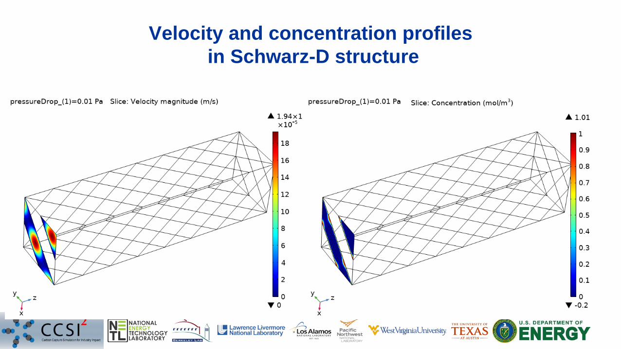
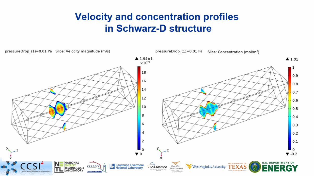
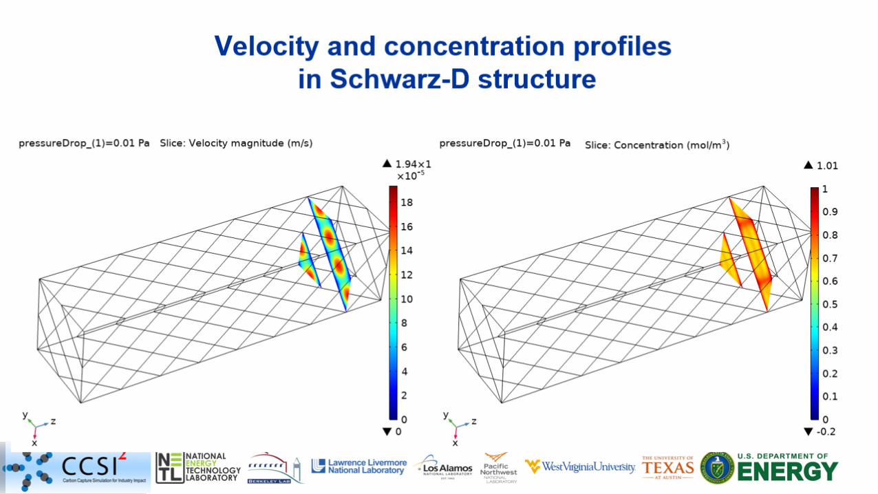
Velocity and concentration profilesin Schwarz-D structure

26

27

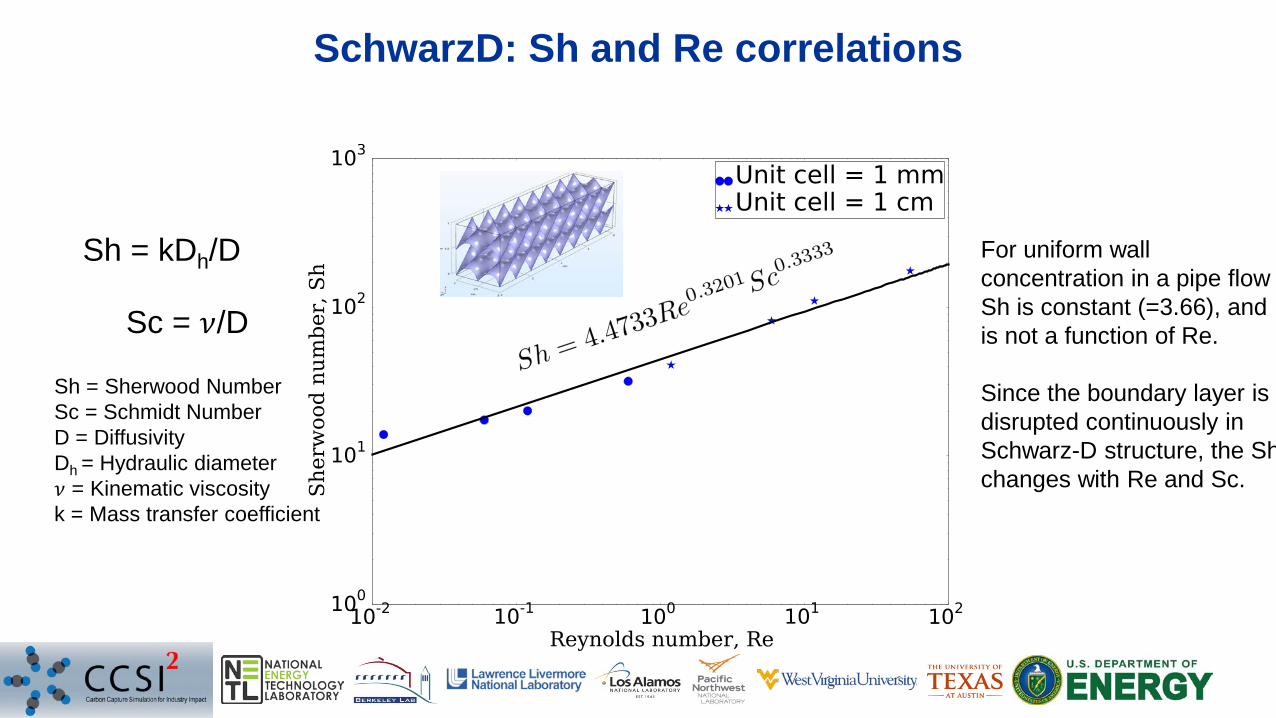
SchwarzD: Sh and Re correlations

Sh = kDh/D

Sc = 𝜈𝜈/D

Sh = Sherwood NumberSc = Schmidt NumberD = DiffusivityDh = Hydraulic diameter𝜈𝜈 = Kinematic viscosityk = Mass transfer coefficient

For uniform wall concentration in a pipe flow Sh is constant (=3.66), and is not a function of Re.

Since the boundary layer is disrupted continuously in Schwarz-D structure, the Shchanges with Re and Sc.

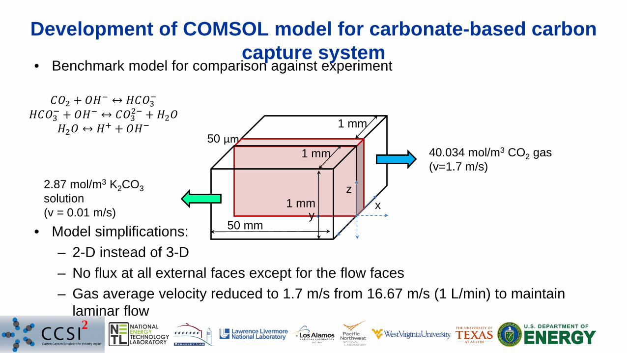
Development of COMSOL model for carbonate-based carbon capture system

• Benchmark model for comparison against experiment

• Model simplifications:– 2-D instead of 3-D– No flux at all external faces except for the flow faces– Gas average velocity reduced to 1.7 m/s from 16.67 m/s (1 L/min) to maintain

laminar flow

1 mm

1 mm

1 mm

50 μm40.034 mol/m3 CO2 gas(v=1.7 m/s)

2.87 mol/m3 K2CO3solution(v = 0.01 m/s) x

y

z

50 mm

𝐶𝐶𝑂𝑂2 + 𝑂𝑂𝐻𝐻− ↔ 𝐻𝐻𝐶𝐶𝑂𝑂3−𝐻𝐻𝐶𝐶𝑂𝑂3− + 𝑂𝑂𝐻𝐻− ↔ 𝐶𝐶𝑂𝑂32− + 𝐻𝐻2𝑂𝑂

𝐻𝐻2𝑂𝑂 ↔ 𝐻𝐻+ + 𝑂𝑂𝐻𝐻−

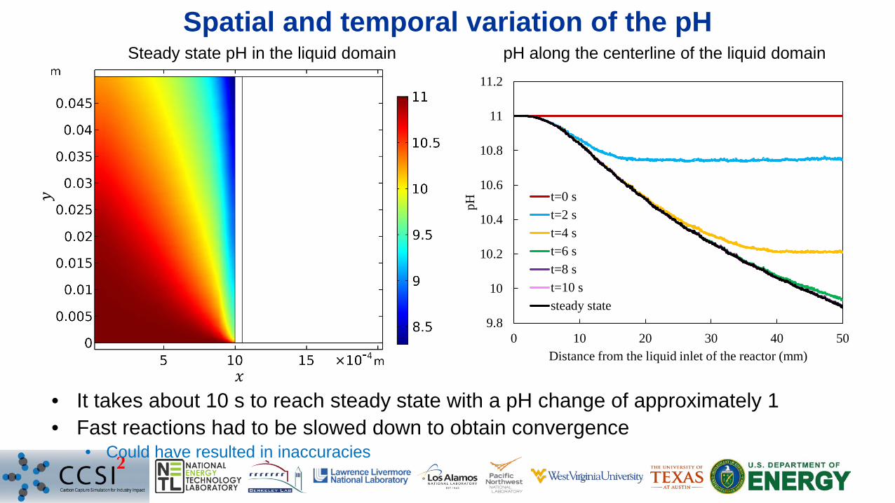
Spatial and temporal variation of the pH

• It takes about 10 s to reach steady state with a pH change of approximately 1• Fast reactions had to be slowed down to obtain convergence

• Could have resulted in inaccuracies

9.8

10

10.2

10.4

10.6

10.8

11

11.2

0 10 20 30 40 50

pH

Distance from the liquid inlet of the reactor (mm)

t=0 st=2 st=4 st=6 st=8 st=10 ssteady state

Steady state pH in the liquid domain pH along the centerline of the liquid domain

𝑥𝑥

𝑦𝑦

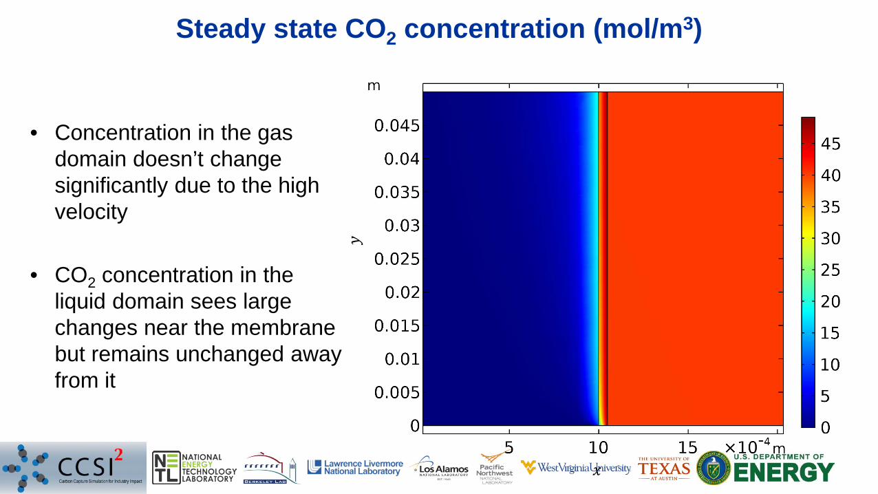
Steady state CO2 concentration (mol/m3)

• Concentration in the gas domain doesn’t change significantly due to the high velocity

• CO2 concentration in the liquid domain sees large changes near the membrane but remains unchanged away from it

𝑥𝑥

𝑦𝑦

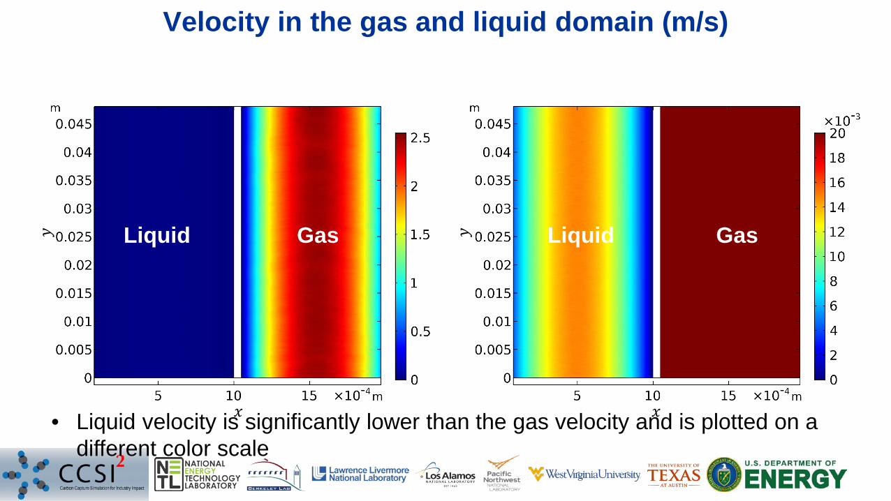
Velocity in the gas and liquid domain (m/s)

• Liquid velocity is significantly lower than the gas velocity and is plotted on a different color scale

𝑥𝑥

𝑦𝑦 GasLiquid GasLiquid

𝑥𝑥

𝑦𝑦

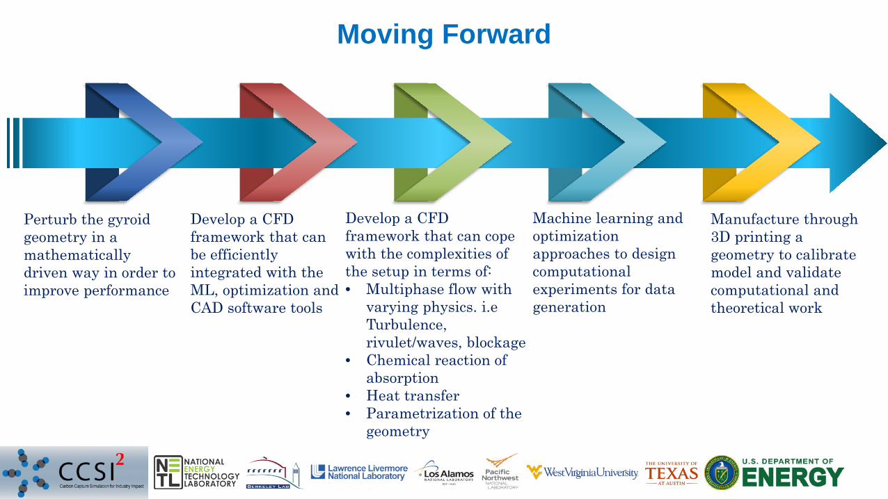
Perturb the gyroidgeometry in a mathematically driven way in order to improve performance

Moving Forward

Develop a CFD framework that can be efficiently integrated with the ML, optimization and CAD software tools

Develop a CFD framework that can cope with the complexities of the setup in terms of:• Multiphase flow with

varying physics. i.eTurbulence, rivulet/waves, blockage

• Chemical reaction of absorption

• Heat transfer• Parametrization of the

geometry

Machine learning and optimization approaches to design computational experiments for data generation

Manufacture through 3D printing a geometry to calibrate model and validate computational and theoretical work

34

Acknowledgments

PNNL: Zhijie Xu, Charlie Freeman, David Heldebrant, Richard Zheng, Rajesh Singh, Jie Bao, Chao Wang, Yucheng FuLLNL: Joshuah Stolaroff, Pratanu Roy, Du Thai Nguyen, Jaisree Iyer Kannan, Brenda Ng, Charles Tong, Wenqin Li NETL: Michael Matuszewski, Benjamin Omell, Joshua Morgan, Grigorios Panagakos UT Austin: Gary Rochelle

Disclaimer: This work is made available as an account of work sponsored by an agency of the United States Government. Neither the UnitedStates Government nor any agency thereof, nor any of their employees, makes any warranty, express or implied, or assumes any legal liability orresponsibility for the accuracy, completeness, or usefulness of any information, apparatus, product, or process disclosed, or represents that its usewould not infringe privately owned rights. Reference herein to any specific commercial product, process, or service by trade name, trademark,manufacturer, or otherwise does not necessarily constitute or imply its endorsement, recommendation, or favoring by the United StatesGovernment or any agency thereof. The views and opinions of authors expressed herein do not necessarily state or reflect those of the UnitedStates Government or any agency thereof.

Carbon Capture Simulation for Industry Impact (CCSI2)

For more informationhttps://www.acceleratecarboncapture.org/

Grigorios Panagakos, Research EngineerCarnegie Mellon University-NETL gpanagak@nandrew.cmu.edu Grigorios.Panagakos@netl.doe.gov