Novel Drying Technology

DIFFUSION DRYING TECHNOLOGY FOR THIN FILM COATING

-ARKA PRABHA ROY

3. LAYOUT CONSIDERATIONS OF DIFFUSION DRYERS

In the following sections we have taken a one-dimensional model of surface coating

(along the Y axis) to predict the diffusive mass transport rate and the time required for the

drying of the solvent.

3.1. THE EQUATIONS AND THE CONSIDERED ONE-DIMENSIONAL LAYER-MODEL

Considering diffusion as the main and only way of mass transport, we get that the rate of

diffusive mass transport depends on the pressure, temperature and their gradients as

following

1 12i i

P TmP x T x

µ• ⎧ ⎫∂ ∂= − −⎨ ⎬

∂ ∂⎩ ⎭

So if we take the mass diffusion transport as the driving cause for the solvent drying

phenomenon, then it seems that the rate of the solvent diffused away depends on the air-

solvent interface pressure, temperature and their gradients. For further simplification the

first term consisting the product of pressure and pressure gradient is neglected in

comparison to the second term consisting the temperature and temperature gradient for

its low order of magnitude. Thus, the expression for the rate of diffusive mass transport looks

like

2dTm

T dyµ•

=

The drying of solvent is considered by the simultaneous effects of the two following

conditions:-

1. Heating through the substrate side due to the higher temperature at the bottom of

the substrate

2. Heat transfer from the upper side of the coating due to the hot wire mesh above

the coating

The basic assumptions taken in account for this one-dimensional model is as following,

Theoretical Considerations of Diffusion Dryers & Experiental Verifications.docx Seite 2 von 6

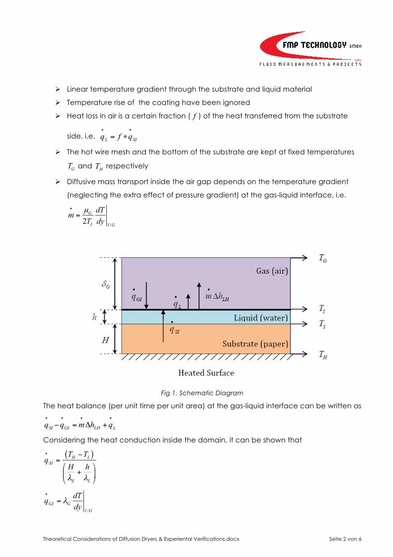
Ø Linear temperature gradient through the substrate and liquid material

Ø Temperature rise of the coating have been ignored

Ø Heat loss in air is a certain fraction ( f ) of the heat transferred from the substrate

side, i.e. L SIq f q• •

= ∗

Ø The hot wire mesh and the bottom of the substrate are kept at fixed temperatures

GT and HT respectively

Ø Diffusive mass transport inside the air gap depends on the temperature gradient

(neglecting the extra effect of pressure gradient) at the gas-liquid interface, i.e.

/2G

I I G

dTmT dyµ•

=

Fig 1. Schematic Diagram

The heat balance (per unit time per unit area) at the gas-liquid interface can be written as

LHSI GI Lq q m h q• • • •

− = Δ +

Considering the heat conduction inside the domain, it can be shown that

( )H ISI

S L

T Tq

H hλ λ

• −=⎛ ⎞

+⎜ ⎟⎝ ⎠

/GGI

I G

dTqdy

λ•

=


Furthermore using the expressions form•

, Lq•

and then re-arranging, we get the balanced

equation as

( ) ( )/ /

12

H I G LHG

II G I G

S L

f T T hdT dTdy T dyH h

µλ

λ λ

− ∗ − Δ+ =

⎛ ⎞+⎜ ⎟

⎝ ⎠

Thus, the temperature gradient at the gas-liquid interface looks like

( ) ( )/

1

2

U I

G LHI GG

I S L

f T TdTdy h H h

Tµ

λλ λ

− ∗ −=

⎛ ⎞⎛ ⎞Δ− ∗ +⎜ ⎟⎜ ⎟

⎝ ⎠ ⎝ ⎠

Now the temperature distribution inside the air-gap (above the coating) satisfies the

energy equation, given by

2

2 0P

G

mCd T dTdy dyλ

•⎛ ⎞⎜ ⎟− =⎜ ⎟⎝ ⎠

Solving we get

1 2 exp P

G

mCT c c yλ

•⎛ ⎞⎜ ⎟= +⎜ ⎟⎝ ⎠

Where 1c and 2c are the two indefinite integration constants, which can be resolved using

the appropriate boundary conditions.

The boundary conditions for the energy equation can be written as

At 0y = , ( ) ( )

/

1

2

H I

G LHI GG

I S L

f T TdTdy h H h

Tµ

λλ λ

− ∗ −=

⎛ ⎞⎛ ⎞Δ− ∗ +⎜ ⎟⎜ ⎟

⎝ ⎠ ⎝ ⎠

At Gy δ= , GT T=

Solving for 1c , 2c and the using these values we get the temperature profile as

( ) ( )1 exp exp

12

P PH I G

G G

GG LH

PG I S L

mC mCf T T y

T Th H hmCT

δλ λ

µλ λ λ

• •

•

⎧ ⎫⎛ ⎞ ⎛ ⎞⎪ ⎪⎜ ⎟ ⎜ ⎟− ∗ − ∗ −⎨ ⎬⎜ ⎟ ⎜ ⎟⎪ ⎪⎝ ⎠ ⎝ ⎠⎩ ⎭= −

⎛ ⎞ ⎛ ⎞Δ∗ − ∗ +⎜ ⎟ ⎜ ⎟⎝ ⎠ ⎝ ⎠


From the above equation the gas-liquid interface temperature ( IT ) is given as; i.e. at 0y = ,

IT T=

( ) ( )1 exp 1

12

PH I G

G

I GG LH

PG I S L

mCf T T

T Th H hmCT

δλ

µλ λ λ

•

•

⎧ ⎫⎛ ⎞⎪ ⎪⎜ ⎟− ∗ − ∗ −⎨ ⎬⎜ ⎟⎪ ⎪⎝ ⎠⎩ ⎭= −

⎛ ⎞ ⎛ ⎞Δ∗ − ∗ +⎜ ⎟ ⎜ ⎟⎝ ⎠ ⎝ ⎠

The mass diffusion rate (per unit area) due to the temperature gradient at the gas-liquid

interface is given by

( ) ( )

( )

1

2

G H I

G LH G IS L

f T Tm

H hh T

µ

µ λλ λ

• − ∗ ∗ −=

⎛ ⎞Δ − ∗ +⎜ ⎟

⎝ ⎠

The drying time for the coating material can be written as

( )

( ) ( )

2

1

L G LH G IS L

dG H I

H hh h TMt

f T Tm

ρ µ λλ λ

µ•

⎛ ⎞∗ ∗ Δ − ∗ +⎜ ⎟

⎝ ⎠= =− ∗ ∗ −

3.2. THEORITICAL PREDICTIONS FOR THE DRYING TIME

Now a sample calculation is done (using Wolfram Mathematica 6.0) for the evaluation of

the mass diffusion rate and the drying time needed for the solvent considering the

following parameter values

H = 300 microns, h = 10 microns, Gδ = 300 microns

f = 0.2 , GT =350K, HT = 295 K

The following material property values are taken as constant with the temperature

variations

Gµ = 51.8 10−× kg/(m.s), Gλ = 0.024W/(m.K), PC = 1.012KJ/(Kg.K)

Lλ = 0.6W/(m.K), Lρ = 1000kg/m3, LHhΔ = 2260 KJ/Kg

Sλ = 0.12W/(m.K)


The mass diffusion rate comes out as 36.63 10−× kg/(m2.s) and the drying time as 1.508 s.

Now the drying time, can be controlled by the two input conditions separately; the

heated surface temperature ( HT ) and the wire mesh temperature ( GT ) above the air gap.

So the analytical study has been done for these two input conditions (keeping one

variable and another fixed at a time) and the results for the gas-liquid interface

temperature, mass diffusion rate and drying time is plotted.

Fig 2(a). Variation of IT with GT Fig 2(b). Variation of IT with HT

Fig 3(a). Variation of m•

with GT Fig 3(b). Variation of m•

with HT

295HT K= 350GT K=

295HT K= 350GT K=


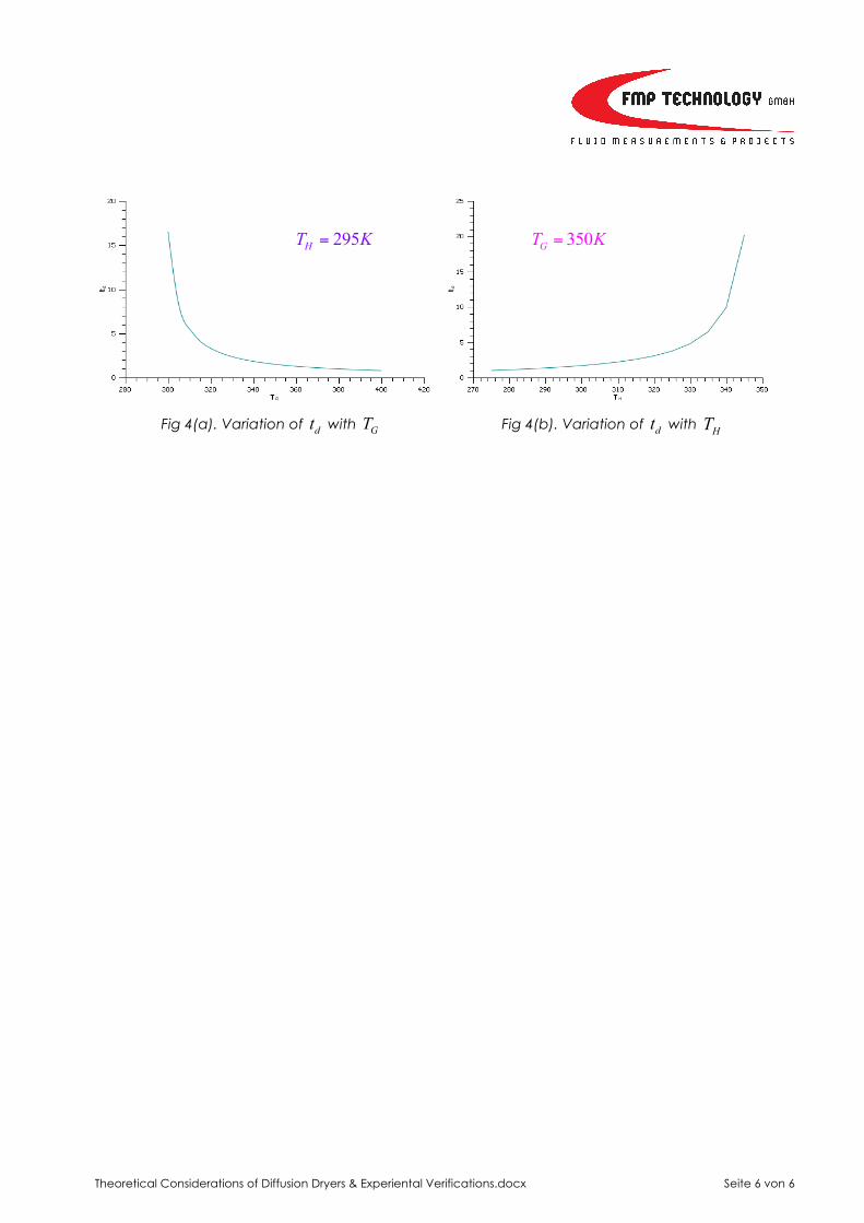
Fig 4(a). Variation of dt with GT Fig 4(b). Variation of dt with HT

295HT K= 350GT K=

Novel Drying Technology

Technology

Transcript of Novel Drying Technology