Klimenta, D. O., et al.: Novel Approach to Analytical Modelling of Steady-State Heat Transfer ... THERMAL SCIENCE: Year 2017, Vol. 21, No. 3, pp. 1529-1542 1529

NOVEL APPROACH TO ANALYTICAL MODELLING OF STEADY-STATE HEAT TRANSFER FROM THE EXTERIOR

OF TEFC INDUCTION MOTORS

by

Dardan O. KLIMENTAa,b* and Antti HANNUKAINEN aa Department of Mathematics and Systems Analysis, Aalto University, Aalto, Finland

b Faculty of Technical Sciences, University of Pristina in Kosovska Mitrovica, Kosovska Mitrovica, Serbia

Original scientific paper https://doi.org/10.2298/TSCI150629091K

The purpose of this paper is to propose a novel approach to analytical modelling of steady-state heat transfer from the exterior of totally enclosed fan-cooled in-duction motors. The proposed approach is based on the geometry simplification methods, energy balance equation, modified correlations for forced convection, the Stefan-Boltzmann law, air-flow velocity profiles, and turbulence factor models. To apply modified correlations for forced convection, the motor exterior is presented with surfaces of elementary 3-D shapes as well as the air-flow velocity profiles and turbulence factor models are introduced. The existing correlations for forced convection from a short horizontal cylinder and correlations for heat transfer from straight fins (as well as inter-fin surfaces) in axial air-flows are modified by intro-ducing the Prandtl number to the appropriate power. The correlations for forced convection from straight fins and inter-fin surfaces are derived from the existing ones for combined heat transfer (due to forced convection and radiation) by using the forced-convection correlations for a single flat plate. Employing the proposed analytical approach, satisfactory agreement is obtained with experimental data from other studies.Key words: analytical model, empirical correlation, energy balance, steady-state

heat transfer, totally enclosed fan-cooled induction motor

Introduction

Existing analytical models of steady-state heat transfer in totally enclosed fan-cooled (TEFC) induction motors are based on a number of commonly accepted assumptions [1-8] and application of the lumped-parameter circuits. However, as the authors will demonstrate, some of these assumptions are unrealistic. In addition, as a rule, analytical modelling of steady-state heat transfer in a solid should begin by setting up only one energy balance equation for its entire outer surface. This was not the case with TEFC induction motors from the first analyt-ical models up to the present day. Therefore, lumped-parameter models may not be accurate enough and adequate for precise modelling of heat transfer processes in electrical machines. In order to accurately model steady-state heat transfer from the motor exterior it is necessary to avoid unrealistic assumptions and lumped-parameters. In the present paper, this is achieved by using the geometry simplification methods, energy balance equation, empirical correlations

* Corresponding author, e-mail: dardan.klimenta@aalto.fi; dardan.klimenta@pr.ac.rs

Klimenta, D. O., et al.: Novel Approach to Analytical Modelling of Steady-State Heat Transfer ... 1530 THERMAL SCIENCE: Year 2017, Vol. 21, No. 3, pp. 1529-1542

(including the Stefan-Boltzmann law), air-flow velocity profiles from [9], and turbulence factor models from [9].

Some of the unrealistic assumptions commonly used in thermal modelling of TEFC induction motors are: (1) that the heat transfer coefficient due to forced convection can only depend on the turbulence factor, Kξ,y, and/or the air-flow velocity at the beginning of the cooling channels, V0 [1-3], (2) that the correlations which were experimentally determined for a combi-nation of forced convection and radiation from [4, 5] can directly be applied to the modelling of only the forced convection as in [3], (3) that the air-flow velocity at the beginning of the cooling channels, V0, always amounts to approximately 70% or 75% of the peripheral velocity of the fan wheel, Vp, [2, 3], (4) that the cooling fins should only increase the heat transfer between the motor exterior and the surroundings [6, 7], which is not consistent with the results presented in [4, 5], (5) that the end-windings do not dissipate heat to the air inside the end-winding zones of the motor, and the heat generated by the stator winding is completely transferred to the stator core [8], etc. In quite a large number of existing analytical models, to a greater or lesser extent, these or similar assumptions adversely affect the model accuracy.

More accurate analytical thermal model should be developed by using: (1) the motor geometry simplification that does not involve changes in the outer surface areas of the frame and end-shields, as well as the motor radius under the cooling fins, (2) the selection of empiri-cal correlations for forced convection appropriate to the particular flow conditions and shapes within the equivalent geometric representation of the motor exterior, (3) a good polynomial approximation to estimate profiles of air-flow velocity, Vy, along the frame cooling channels [9], and (4) an appropriate model to estimate reduction of the turbulence factor, Kξ,y,along the frame cooling channels [9].

The thermal model proposed in this paper is based on a simplified geometric represen-tation of the exterior of TEFC induction motors under different load conditions by using surfac-es of elementary 3-D shapes. The model proposed in this paper considers an equivalent com-bination/representation of surfaces of 3-D geometric shapes to simplify the exterior of TEFC induction motors operating under different loads. All the surfaces have their own heat transfer coefficients due to forced convection and radiation. The coefficients represent unknowns in the energy balance equation and their values have been estimated with the appropriate empirical correlations. Moreover, the suggested approach to thermal modelling has been applied to two TEFC induction motors having different pole numbers, shaft heights, and rated powers; both operating in two different regimes.

Equivalent geometric representation of the motor exterior

From an empirical point of view, pulley, metal nameplate, eyebolt, metal keys of the shaft, fan wheel and cowl do not have a significant effect on the heat transfer between the motor exterior and the surroundings. Hence, these elements additionally complicate the equivalent geometric representation of the motor shape. For this reason, the elements are not included into the present geometric model.

Forced convection and radiation from the shaft extensions are disabled by the pulley and the fan wheel. Therefore, the surfaces of the shaft extensions are assumed to be cylindrical and adiabatic. Motor elements such as terminal box and mounting feet have complex shapes and outer surface areas of considerable sizes. These two elements are difficult to model ther-mally and geometrically, and their effect can not be ignored. Moreover, end-shields are usually hollow (the shaft passes through the end-shields), externally-finned and not ideally flat and/or cylindrical.

Klimenta, D. O., et al.: Novel Approach to Analytical Modelling of Steady-State Heat Transfer ... THERMAL SCIENCE: Year 2017, Vol. 21, No. 3, pp. 1529-1542 1531

Modelling the geometry of the TEFC induction motor elements (main parts and those with significant surfaces) for the purpose of their thermal analysis will be based on empirically confirmed facts. These empirical facts are: (1) if there is any change in the motor outer surface during the procedure of geometry modelling, its heat transfer coefficients need to be recalcu-lated accordingly [10], (2) a change in the number of cooling fins up to 12 and an appropriate change in the spacing between the fins do not affect significantly their heat transfer coefficients [6, 7], (3) a small change in the height of cooling fins with regard to its optimal value will not have significant effect on the fin efficiency [11] and corresponding heat transfer coefficients [6, 7], (4) a change in the number of cooling fins will not cause any significant change in the air-flow velocity at the beginning of the cooling channels, V0 [6, 7], (5) the one-nth-power law can be applied in a case of air-flow through the annular gap between two coaxial tubes [12-15], and (6) the degree of flow turbulence depends very little on the air-flow velocity [16].

In order to simplify the geometry of a TEFC induction motor, its shape is represented by a union of rotating and stationary horizontal cylinders with and without fins, where a num-ber of lengths and one radius differ from the corresponding actual dimensions. In the following paragraphs and equations, radii, riE, lengths/thicknesses, LiE, and surfaces, SiE, labelled with a combination of surface numbers i = 1-10 and capital letter E differ from the corresponding actual dimensions of the motor. Radii, ri, lengths/thicknesses, Li, and surfaces, Si, labelled only with surface numbers i = 1-10 are introduced in order to display the equations related to the steady-state heat transfer model in a more convenient manner. The surface numbers i = 1-10 (that is, subscripts) are used for the labelling as shown in fig. 1. All radii and lengths are in meters, and surface areas are in m2.

The exterior of a TEFC induction motor, in the direction of fan wheel from the drive end of the shaft, is represented by a combination of surfaces composed of: (S1) the base surface of a rotating disk having radius r1, thickness L1 = 0 m and base area S1, (S2) the lateral surface of a rotating horizontal cylinder having radius r2 = r1, length L2 = L2E and lateral area S2 = S2E, (S3) the ring-shaped base surface of a stationary horizontal hollow cylinder having outer radi-us r3, length L3 = L3E and base area S3 = S3E, (S4) the lateral surface of a stationary horizontal cylinder having radius r4, length L4 = L3E and lateral area S4 = S4E, (S5) all the fin surfaces of a stationary horizontal longitudinally-finned cylinder having radius over the fins r5 = r5E, length L5 and total fin area S5 = S5E, (S6) all the inter-fin surfaces of a stationary horizontal longitudi-nally-finned cylinder having radius under the fins r6 = r3, length L6 = L5 and total inter-fin area S6 = S6E, (S7) the lateral surface of a stationary horizontal cylinder having radius r7 = r3, length L7 = L7E and lateral area S7 = S7E,, (S8) the ring-shaped base surface of a stationary horizontal

Figure 1. Equivalent TEFC induction motor; (a) side view, (b) view from the drive end side

(a) (b)

Drive end side

Non-drive end side

xy

x

y

Klimenta, D. O., et al.: Novel Approach to Analytical Modelling of Steady-State Heat Transfer ... 1532 THERMAL SCIENCE: Year 2017, Vol. 21, No. 3, pp. 1529-1542

hollow cylinder having outer radius r8 = r3, length L8 = L7E and base area S8 = S8E, (S9) the lateral surface of a rotating horizontal cylinder having radius r9, length L9 = L9E and lateral area S9 = S9E, and (S10) the base surface of a rotating disk having radius r10 = r9, thickness L10 = 0 m and base area S10. Equivalent geometric representation of a TEFC induction motor by using the S1, S2, …, S9 and S10 surfaces, that is, the equivalent TEFC induction motor is shown in fig. 1.

The equivalent dimensions are determined such that surface areas of the equivalent geometric representations of the frame and end-shields match with the actual surface areas of the same elements. According to this principle, S3E + S4E is the actual outer surface area of the drive end-shield, S7E + S8E is the actual outer surface area of the non-drive end-shield, and S3E is equal to S8E. Moreover, S5E + S6E is the actual outer surface area of the finned frame, terminal box and two mounting feet.

Basic calculations lead to the following formulas:

2 3'E EL L L= − (1)

2 2

3 4 3 93

3

( )2

E EE

S S r rLr

+ − π −=

π (2)

2 2

7 8 3 97

3

( )2

E EE

S S r rLr

+ − π −=

π (3)

9 2 3 5 7E E E EL L L L L L= − − − − (4)

5 3E FEr r H= + (5)

where L' is the distance from the flat surface of the drive shaft extension to the end of the cool-ing channels, L – the length of the shaft, and HFE – the height of the equivalent cooling fins in m, which according to fig. 1(b) is:

5 6 3 5

5

22

E EFE

FE

S S r LHL N

+ − π= (6)

where NFE is the number of the equivalent cooling fins (an integer value). Also, according to fig. 1(b), the width of the equivalent cooling channels (that is, the spacing between equivalent fins) at half the height HFE in meters is:

22 1 cos2

EFE mE FD r α= − − ∆ (7)

where rmE = (r3 + r5E)/2 is the radius of the circle which divides the equivalent fins into two halves, ΔF – the thickness of an actual cooling fin, and αE = 360/NFE – the angle between the radial axes of every two adjacent equivalent fins in degrees. The radial axis of an equivalent fin represents a straight line passing through the center points of the shaft and the equivalent fin. Moreover, in accordance with fig. 1, x is the distance from the fin base measured along the radial axis in m.

Model for steady-state heat transfer from the motor exterior

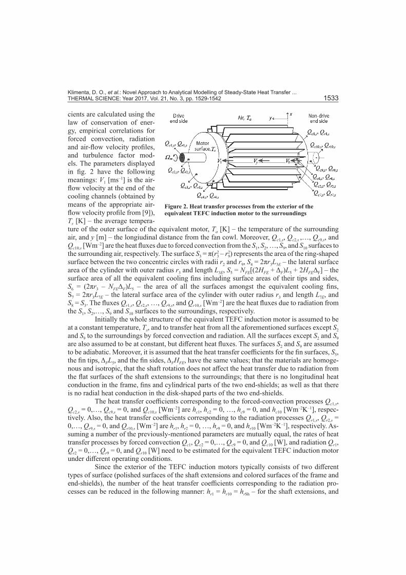
The steady-state heat transfer from the exterior of the equivalent TEFC induction motor is discussed in this section and illustrated in fig. 2. The average values of the heat transfer coeffi-

Klimenta, D. O., et al.: Novel Approach to Analytical Modelling of Steady-State Heat Transfer ... THERMAL SCIENCE: Year 2017, Vol. 21, No. 3, pp. 1529-1542 1533

cients are calculated using the law of conservation of ener-gy, empirical correlations for forced convection, radiation and air-flow velocity profiles, and turbulence factor mod-els. The parameters displayed in fig. 2 have the following meanings: V1 [ms–1] is the air-flow velocity at the end of the cooling channels (obtained by means of the appropriate air-flow velocity profile from [9]), Ts [K] – the average tempera-ture of the outer surface of the equivalent motor, Ta [K] – the temperature of the surrounding air, and y [m] – the longiudinal distance from the fan cowl. Moreover, Qc1,s, Qc2,s ,…, Qc9,s, and Qc10,s [Wm–2] are the heat fluxes due to forced convection from the S1, S2, …, S9, and S10 surfaces to the surrounding air, respectively. The surface S3 = π(r2

3 – r29) represents the area of the ring-shaped

surface between the two concentric circles with radii r2 and r9, S4 = 2πr3L3E – the lateral surface area of the cylinder with outer radius r3 and length L3E, S5 = NFE[(2HFE + ΔF)L5 + 2HFEΔF] – the surface area of all the equivalent cooling fins including surface areas of their tips and sides, S6 = (2πr3 – NFEΔF)L5 – the area of all the surfaces amongst the equivalent cooling fins, S7 = 2πr3L7E – the lateral surface area of the cylinder with outer radius r3 and length L7E, and S8 = S3. The fluxes Qr1,s, Qr2,s, …, Qr9,s, and Qr10,s [Wm–2] are the heat fluxes due to radiation from the S1, S2,…, S9 and S10 surfaces to the surroundings, respectively.

Initially the whole structure of the equivalent TEFC induction motor is assumed to be at a constant temperature, Ts, and to transfer heat from all the aforementioned surfaces except S2 and S9 to the surroundings by forced convection and radiation. All the surfaces except S2 and S9 are also assumed to be at constant, but different heat fluxes. The surfaces S2 and S9 are assumed to be adiabatic. Moreover, it is assumed that the heat transfer coefficients for the fin surfaces, S5, the fin tips, ΔFL5, and the fin sides, ΔFHFE, have the same values; that the materials are homoge-nous and isotropic, that the shaft rotation does not affect the heat transfer due to radiation from the flat surfaces of the shaft extensions to the surroundings; that there is no longitudinal heat conduction in the frame, fins and cylindrical parts of the two end-shields; as well as that there is no radial heat conduction in the disk-shaped parts of the two end-shields.

The heat transfer coefficients corresponding to the forced-convection processes Qc1,s, Qc2,s = 0,…, Qc9,s = 0, and Qc10,s [Wm–2] are hc1, hc2 = 0, …, hc9 = 0, and hc10 [Wm–2K–1], respec-tively. Also, the heat transfer coefficients corresponding to the radiation processes Qr1,s, Qr2,s = 0,…, Qr9,s = 0, and Qr10,s [Wm–2] are hr1, hr2 = 0, …, hr9 = 0, and hr10 [Wm–2K–1], respectively. As-suming a number of the previously-mentioned parameters are mutually equal, the rates of heat transfer processes by forced convection Qc1, Qc2 = 0,…, Qc9 = 0, and Qc10 [W], and radiation Qr1, Qr2 = 0,…, Qr9 = 0, and Qr10 [W] need to be estimated for the equivalent TEFC induction motor under different operating conditions.

Since the exterior of the TEFC induction motors typically consists of two different types of surface (polished surfaces of the shaft extensions and colored surfaces of the frame and end-shields), the number of the heat transfer coefficients corresponding to the radiation pro-cesses can be reduced in the following manner: hr1 = hr10 = hrSh – for the shaft extensions, and

Figure 2. Heat transfer processes from the exterior of the equivalent TEFC induction motor to the surroundings

Klimenta, D. O., et al.: Novel Approach to Analytical Modelling of Steady-State Heat Transfer ... 1534 THERMAL SCIENCE: Year 2017, Vol. 21, No. 3, pp. 1529-1542

hr3 = hr4 = hr5 = hr6 = hr7 = hr8 = hrF – for the frame and end-shields. The heat transfer coefficients hrSh and hrF correspond with the appropriate thermal emission coefficients εSh and εF, respectively.

The iteration procedure for calculation of the heat transfer coefficients requires knowl-edge of Ts, which is initially unknown. To obtain an initial estimate of Ts, the same numeri-cal value should be taken for all unknown heat transfer coefficients (for example 50 W/m2K). Therefore, an initial estimate of Ts can be obtained from:

10

tot , ,1

( )ci s ri s ii

Q Q Q S=

= +∑ (8)

More precisely:

tots a

c r

QT T= +Σ + Σ

(9)

where

10 10

1 1, ,c ci i r ri i

i ih S h S

= =

Σ = Σ =∑ ∑

and Qtot [W] is the total amount of power lost within the TEFC induction motor. The total pow-er loss Qtot is usually measured and consists of the following five components [17]: the stator winding losses, the iron-core losses, the rotor winding losses, the friction and windage losses and the stray losses.

The heat fluxes due to forced convection from the outer surfaces of the motor to the surrounding air are modelled in a usual manner by an equation of the form:

, ( )ci s ci s aQ h T T= − (10)

where Qci,s and hci represent one of the aforementioned heat fluxes due to forced convection and its corresponding heat transfer coefficient.

The forced-convection heat transfer coefficients, hci, equal:

Nu Nu tci

c

K khL

= (11)

where KNu is the dimensionless coefficient which equals 1 for laminar and turbulent forced con-vection from all the aforementioned surfaces except for turbulent forced convection from the flat and cylindrical surfaces of end-shields, Nu – the average Nusselt number which should be calculated using different empirical correlations, kt [Wm–1K–1] – the thermal conductivity of the surrounding air, and Lc [m] – an appropriate characteristic length. The values of coefficient KNu for turbulent forced convection from the end-shields in this iteration procedure are specified in the following manner [9]:

4.62Nu , 1 (1.4163 1)e for flat outer surfaces of end-shields,y

yK Kξ−= = + − − (12)

and

13.087Nu , 1 (1.6776 1)e for cylindrical outer surfaces of end-shieldsy

yK Kξ−= = + − − (13)

where Kξ,y is the turbulence factor model. At a film temperature Tf = (Ts + Ta)/2, the thermal conductivity, kt, the kinematic viscosity, ν [m2s–1], and the Prandtl number of air have been read from corresponding input data files and interpolated using a cubic spline.

Klimenta, D. O., et al.: Novel Approach to Analytical Modelling of Steady-State Heat Transfer ... THERMAL SCIENCE: Year 2017, Vol. 21, No. 3, pp. 1529-1542 1535

The average Nusselt number correlations for 3-D shapes which are used to represent the motor exterior, together with the corresponding characteristic lengths, Lc, Reynolds num-bers, and references, are presented in tab. 1. Some of these correlations are modified by intro-ducing the Prandtl number to the appropriate power, while others are derived from existing ones for combined heat transfer by using the forced-convection correlations for a single flat plate.

The heat fluxes due to radiation from all the particular outer surfaces of the motor to the surroundings are modelled by the Stefan-Boltzmann law, that is, by the following equation:

, ( )ri s ri s aQ h T T= − (14)

where Qri,s is one of the aforementioned heat fluxes due to radiation and hri is corresponding heat transfer coefficient, which depends on temperature in the following manner:

2 2SB ( )( )ri i s a s ah T T T Tσ ε= + + (15)

where σSB is the Stefan-Boltzmann constant and εi is the appropriate thermal emission coeffi-cient (εi equals to εSh, εF or zero).

Moreover, from iteration to iteration the coefficients hci and hri should be calculated using eqs. (11) and (15), respectively. Each new estimation for Ts should be calculated by av-eraging the previously estimated and newly found values of hci and hri. The iteration procedure continues until the difference between the previously estimated and the newly found Ts becomes sufficiently small. Finally, this iteration procedure uses the final value of Ts to calculate the final values of hci, hri, Qci = Qci,sSi and Qri = Qri,sSi where Qci, Qri, and Si are one of the aforementioned heat transfer rates due to forced convection, one of the aforementioned heat transfer rates due to radiation and corresponding surface area, respectively.

When all the heat transfer rates due to forced convection and radiation are known, it is possible to determine the temperature distribution along the frame. In order to obtain the best possible longitudinal temperature profile, the following assumptions are also introduced: (1) temperatures of the drive and non-drive end-shields Ts1 and Ts0 are constant, unequal, Ts1 is greater than Ts0 and it always holds that Ts1 > Ts > Ts0, (2) longitudinal temperature profiles Ts(y) for the cooling fins and inter-fin surfaces have the same shapes and change with the distance y within the range from Ts0 to Ts1, (3) maximum surface temperature along the frame TsM and its corresponding longitudinal co-ordinate yM are available based on infrared thermography or any other measurement technique, (4) temperatures of the shaft extensions are equal to the tempera-tures of the appropriate end-shields, and (5) all the heat transfer coefficients due to radiation are constant and depend only on the average temperature Ts.

In accordance with these assumptions for the given TsM [K] and yM [m], the following expression for the longitudinal temperature profile Ts(y) [°C] is obtained:

( ) 273.157[ ( ) ]

cj rjs a

cj rj j

Q QT y T

h y h S+

= + −+ (16)

where

,

, ,,

( )( )

M

y cj rjcj y cj rj

y j sM a

K Q Qh y K h h

K S T Tξ

ξξ

∞

+= = −

− (17)

Klimenta, D. O., et al.: Novel Approach to Analytical Modelling of Steady-State Heat Transfer ... 1536 THERMAL SCIENCE: Year 2017, Vol. 21, No. 3, pp. 1529-1542

Table 1. Forced-convection correlations for elementary 3-D shapes

Geometry Flow regime

Recommended correlation

Lc Reynolds number and intended range of its application

Ref.No. 3-D shape Sur-face [m]

1*a Rotating disk S1

Laminar1/ 2

1/3

0.4964ReNu0.6/ Pr 0.95/ Pr

=+

r1

251Re 2.4 10rΩ

ν= < ⋅ [18-20]

Turbulent 4 5 1 3Nu 0 0168Re Pr/ /.= r1

251Re 2.4 10rΩ

ν= ≥ ⋅ [18-20]

3*bStationary horizontal cylinder

S3

Laminar0.656 1 3Nu 0.108Re Pr /= 2r3

41 32Re 6 10V rν

= < ⋅

[21-23]Turbulent 41 32Re 6 10V r

ν= ≥ ⋅

4*bStationary horizontal cylinder

S4

Laminar0.682 1 3Nu 0.137Re Pr /= 2r3

41 32Re 6 10V rν

= < ⋅

[21]Turbulent 41 32Re 6 10V r

ν= ≥ ⋅

5*c

Stationary horizontal

finned cylinder

S5

Laminar

L540 5Re 6 10V L

ν= < ⋅ [4, 5,

24]

(2) 0.02Nu Nu 1 FE

FE

HD

= −

1/3

(2) (1)Nu Nu 1 0.12 FE

FE

HD

= −

(1) 1/ 2 1 3Nu 0.664Re Pr /=

Turbulent

L540 5Re 6 10V L

ν= ≥ ⋅ [4, 5,

24]

(2) 0.02Nu Nu 1 FE

FE

HD

= −

1/ 2

(2) (1)Nu Nu 1 0.09 FE

FE

HD

= −

(1) 4/5 1 3Nu 0.037Re Pr /=

6*c

Stationary horizontal

finned cylinder

S6

Laminar

L540 5Re 6 10V L

ν= < ⋅ [4, 5,

24]

1/3(1)Nu Nu 1 0.35 FE

FE

HD

= −

(1) 1/ 2 1 3Nu 0.664Re Pr /=

Turbulent

L540 5Re 6 10V L

ν= ≥ ⋅ [4, 5,

24]

1/ 2(1)Nu Nu 1 0.23 FE

FE

HD

= −

(1) 4/5 1 3Nu 0.037Re Pr /=

→

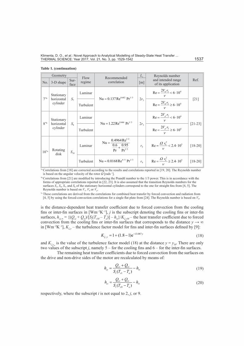
Klimenta, D. O., et al.: Novel Approach to Analytical Modelling of Steady-State Heat Transfer ... THERMAL SCIENCE: Year 2017, Vol. 21, No. 3, pp. 1529-1542 1537

Geometry Flow regime

Recommended correlation

Lc Reynolds number and intended range of its application

Ref.No. 3-D shape Sur-face [m]

7*bStationary horizontal cylinder

S7

Laminar0.682 1 3Nu 0.137Re Pr /= 2r3

40 32Re 6 10V rν

= < ⋅

[21]Turbulent 40 32Re 6 10V r

ν= ≥ ⋅

8*bStationary horizontal cylinder

S8

Laminar0.466 1 3Nu 1.22Re Pr /= 2r3

3 42Re 6 10pV r

ν= < ⋅

[21-23]

Turbulent 3 42Re 6 10pV r

ν= ≥ ⋅

10*a Rotating disk S10

Laminar

1/ 2

1/3

0.4964ReNu 0.6 0.95Pr Pr

=+ r9

259Re 2.4 10rΩ

ν= < ⋅ [18-20]

Turbulent 4 5 1 3Nu 0 0168Re Pr/ /.= r9

259Re 2.4 10rΩ

ν= ≥ ⋅ [18-20]

*a Correlations from [18] are corrected according to the results and correlations reported in [19, 20]. The Reynolds number is based on the angular velocity of the rotor Ω [rads–1].

*b Correlations from [21] are modified by introducing the Prandtl number to the 1/3 power. This is in accordance with the forms of appropriate correlations reported in [22, 23]. It is also assumed that the transition Reynolds numbers for the surfaces S3, S4, S7, and S8 of the stationary horizontal cylinders correspond to the one for straight fins from [4, 5]. The Reynolds number is based on V1, V0 or Vp.

*c These correlations are derived from the correlations for combined heat transfer by forced convection and radiation from [4, 5] by using the forced-convection correlations for a single flat plate from [24]. The Reynolds number is based on V0.

is the distance-dependent heat transfer coefficient due to forced convection from the cooling fins or inter-fin surfaces in [Wm–2K–1], j is the subscript denoting the cooling fins or inter-fin surfaces, hcj,∞ = (Qcj + Qrj)/[Sj(TsM – Ta)] – hrj/Kξ,yM – the heat transfer coefficient due to forced convection from the cooling fins or inter-fin surfaces that corresponds to the distance y → ∞ in [Wm–2K–1], Kξ,y – the turbulence factor model for fins and inter-fin surfaces defined by [9]:

13.087, 1 (1.8 1)e yyKξ

−= + − (18)

and Kξ,yM is the value of the turbulence factor model (18) at the distance y = yM. There are only

two values of the subscript j, namely 5 – for the cooling fins and 6 – for the inter-fin surfaces. The remaining heat transfer coefficients due to forced convection from the surfaces on

the drive and non-drive sides of the motor are recalculated by means of:

1( )

ci rici ri

i s a

Q Qh hS T T

+= −

− (19)

0( )

ci rici ri

i s a

Q Qh hS T T

+= −

− (20)

respectively, where the subscript i is not equal to 2, j, or 9.

Table 1. (continuation)

Klimenta, D. O., et al.: Novel Approach to Analytical Modelling of Steady-State Heat Transfer ... 1538 THERMAL SCIENCE: Year 2017, Vol. 21, No. 3, pp. 1529-1542

Results and discussions

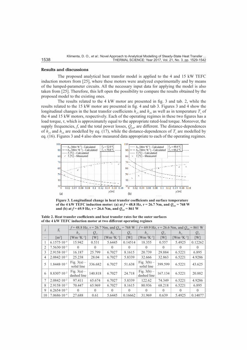
The proposed analytical heat transfer model is applied to the 4 and 15 kW TEFC induction motors from [25], where these motors were analyzed experimentally and by means of the lumped-parameter circuits. All the necessary input data for applying the model is also taken from [25]. Therefore, this left open the possibility to compare the results obtained by the proposed model to the existing ones.

The results related to the 4 kW motor are presented in fig. 3 and tab. 2, while the results related to the 15 kW motor are presented in fig. 4 and tab 3. Figures 3 and 4 show the longitudinal changes in the heat transfer coefficients hc5 and hc6 as well as in temperature Ts of the 4 and 15 kW motors, respectively. Each of the operating regimes in these two figures has a load torque, τ, which is approximately equal to the appropriate rated-load torque. Moreover, the supply frequencies, f, and the total power losses, Qtot, are different. The distance-dependences of hc5 and hc6 are modelled by eq. (17), while the distance-dependences of Ts are modelled by eq. (16). Figures 3 and 4 also show measured data appropriate to each of the operating regimes.

Figure 3. Longitudinal change in heat transfer coefficients and surface temperature of the 4 kW TEFC induction motor: (a) at f = 48.8 Hz, τ = 26.7 Nm, and Qtot = 768 W and (b) at f = 69.9 Hz, τ = 26.6 Nm, and Qtot = 861 W

hc5 [Wm–2K–1] – Calculatedhc6 [Wm–2K–1] – CalculatedTs [°C] – CalculatedTs [°C] – Measured

Ts0 = 52.9 °CTs1 = 70.8 °C

y [m] y [m](a) (b)

hc5 [Wm–2K–1] – Calculatedhc6 [Wm–2K–1] – CalculatedTs [°C] – CalculatedTs [°C] – Measured

Ts0 = 49.4 °CTs1 = 66.2 °C

Table 2. Heat transfer coefficients and heat transfer rates for the outer surfaces of the 4 kW TEFC induction motor at two different operating regimes

i Sif = 48.8 Hz, τ = 26.7 Nm, and Qtot = 768 W f = 69.9 Hz, τ = 26.6 Nm, and Qtot = 861 W

hci Qci hri Qri hci Qci hri Qri

– [m2] [Wm–2K–1] [W] [Wm–2K–1] [W] [Wm–2K–1] [W] [Wm–2K–1] [W]1 6.1575∙10–4 15.942 0.531 5.6445 0.14514 18.355 0.557 5.4925 0.122622 7.5630∙10–3 0 0 0 0 0 0 0 03 2.9158∙10–2 16.187 25.799 6.7027 8.1615 20.739 29.884 6.5221 6.8954 2.0842∙10–2 25.238 28.04 6.7027 5.8339 32.666 32.863 6.5221 4.9286

5 1.8448∙10–1 Fig. 3(a) – solid line 336.682 6.7027 51.638 Fig. 3(b) –

solid line 399.599 6.5221 43.625

6 8.8307∙10–2 Fig. 3(a) – dashed line 140.818 6.7027 24.718 Fig. 3(b) –

dashed line 167.134 6.5221 20.882

7 2.0842∙10–2 97.411 65.674 6.7027 5.8339 122.62 74.349 6.5221 4.92868 2.9158∙10–2 70.447 65.969 6.7027 8.1615 80.936 68.218 6.5221 6.8959 6.2654∙10–3 0 0 0 0 0 0 0 010 7.0686∙10–4 27.688 0.61 5.6445 0.16662 31.969 0.639 5.4925 0.14077

Klimenta, D. O., et al.: Novel Approach to Analytical Modelling of Steady-State Heat Transfer ... THERMAL SCIENCE: Year 2017, Vol. 21, No. 3, pp. 1529-1542 1539

Generally, the length of the frame can be divided into three zones: drive end-winding, stator core, and non-drive end-winding. The lengths of the drive and non-drive end-winding zones are approximately equal to each other and these lengths amount to 0.035 and 0.07 m for the 4 and 15 kW motors, respectively. The lengths of the stator core zones of the 4 and 15 kW motors are 0.105 and 0.23 m, respectively. Accordingly, the results shown in figs. 3 and 4 indicate that a good agreement exists between the calculated and measured data for the stator core zones of both motors. The percent deviations between the measured data and the data ob-tained by the proposed analytical model for stator core zones are lower than 12.5% for the 4 kW motor and lower than 6.3% for the 15 kW motor. Similarly, for end-winding zones, the percent deviations are between 3.7~17.2% for the 4 kW motor and between 6 ~ 10.9% for the 15 kW motor. Based on the results shown in these figures, it can also be seen that the percent deviation gradually increases as the supply frequency (that is, the angular velocity of the rotor) increases.

Tables 2 and 3 summarize the analytical results obtained for all the operating regimes of the 4 and 15 kW motors. For each operating regime a set of 15 to 17 iterations was need-ed. The heat transfer coefficients and the heat transfer rates are calculated using a MATLAB

Table 3. Heat transfer coefficients and heat transfer rates for the outer surfaces of the 15 kW TEFC induction motor at two different operating regimes

i Sif = 47.9 Hz, τ = 148 Nm, and Qtot = 2631 W f = 29.7 Hz, τ = 147 Nm, and Qtot = 2039 W

hci Qci hri Qri hci Qci hri Qri

– [m2] [Wm–2K–1] [W] [Wm–2K–1] [W] [Wm–2K–1] [W] [Wm–2K–1] [W]1 1.8096∙10–3 10.39 1.267 5.6421 0.42549 8.0824 1.056 5.7295 0.464282 2.0029∙10–2 0 0 0 0 0 0 0 03 6.8534∙10–2 12.73 58.528 6.6998 19.136 8.7454 43.948 6.8037 20.8814 5.1466∙10–2 21.635 70.683 6.6998 14.37 14.914 52.317 6.8037 15.681

5 8.1121∙10–1 Fig. 4(a) – solid line 1391.432 6.6998 226.5 Fig. 4(b) –

solid line 986.052 6.8037 247.16

6 3.0496∙10–1 Fig. 4(a) – dashed line 446.9 6.6998 85.15 Fig. 4(b) –

dashed line 316.7 6.8037 92.915

7 5.1466∙10–2 84.254 154.992 6.6998 14.37 58.631 116.866 6.8037 15.6818 6.8534∙10–2 52.637 127.997 6.6998 19.136 41.21 108.633 6.8037 20.8819 1.0653∙10–2 0 0 0 0 0 0 0 010 1.9635∙10–3 20.203 1.374 5.6421 0.46168 15.619 1.146 5.7295 0.50378

Figure 4. Longitudinal change in heat transfer coefficients and surface temperature of the 15 kW TEFC induction motor: (a) at f = 47.9 Hz, τ = 148 Nm, and Qtot = 2631 W, and (b) at f = 29.7 Hz, τ = 147 Nm, and Qtot = 2039 W

y [m] y [m](a) (b)

hc5 [Wm–2K–1] – Calculatedhc6 [Wm–2K–1] – CalculatedTs [°C] – CalculatedTs [°C] – Measured

Ts0 = 56.2 °CTs1 = 78.3 °C

hc5 [Wm–2K–1] – Calculatedhc6 [Wm–2K–1] – CalculatedTs [°C] – CalculatedTs [°C] – Measured

Ts0 = 59.4 °CTs1 = 80.8 °C

Klimenta, D. O., et al.: Novel Approach to Analytical Modelling of Steady-State Heat Transfer ... 1540 THERMAL SCIENCE: Year 2017, Vol. 21, No. 3, pp. 1529-1542

program. From the simulation results it can be noticed that the average temperature, Ts, equals to 61.76, 56.257, 61.675, and 64.781 °C for the operating regime presented in figs. 3(a), 3(b), 4(a), and 4(b) (at the air temperature Ta = 20 °C), respectively. From the same simulations it can be noticed that the average values of the coefficients hc5 and hc6 equal to: 43.701 and 38.186 W/m2K – for the regime presented in fig. 3(a), 59.741 and 52.201 W/m2K – for the re-gime presented in fig. 3(b), 41.158 and 35.163 W/m2K – for the regime presented in fig. 4(a), 27.144 and 23.19 W/m2K – for the regime presented in fig. 4(b), respectively. Moreover, the temperature TsM and its corresponding coordinate yM are taken from measured data, figs. 3(a), 3(b), 4(a) and 4(b).

In comparison with the result calculated by the lumped-parameter circuit from [25], the average temperature Ts = 61.675 °C of the 15 kW motor at rated load conditions is lower by 8.125 °C. However, that is not the case with the 4 kW motor at rated load conditions. For the 4 kW motor at rated load conditions this difference is only 0.16 °C. Further comparison of differences between these two models would be unnecessary.

By knowing the amounts of heat dissipated through the end-shields, it is possible to calculate all the heat transfer coefficients of the motor exterior with a satisfactory accuracy [25]. According to [25], the amounts of heat dissipated through the drive and non-drive end-shields, respectively, are 9, and 19% of Qtot for the 4 kW motor at rated operation, and 6, and 12% of Qtot for the 15 kW motor at rated operation. According to tabs. 2 and 3, the portions of heat dissipat-ed through the drive and non-drive end-shields amount to: (1) 8.833% and 18.963% – for the regime presented in fig. 3(a), (2) 8.661% and 17.932% – for the regime presented in fig. 3(b), (3) 6.185% and 12.029% – for the regime presented in fig. 4(a), and (4) 6.514% and 12.852% – for the regime presented in fig. 4(b). The portions (1) and (3) agree well with the corresponding data given in [25]. Moreover, it can be noticed that the portions of heat dissipated through the end-shields decrease as the supply frequency increases (or increase as f decreases).

Conclusions

The conclusions arising from the present paper are as follows. y The proposed approach to analytical modelling of steady-state heat transfer from the ex-

terior of TEFC induction motors excludes rough approximations, it is scientifically and empirically based, rather simple and provides more accurate results in comparison with the common ones, which are based on the lumped-parameter circuits.

y The procedure for modelling the geometry of TEFC induction motors is based on empiri-cally confirmed facts and its implementation does not require a large amount of input data.

y A set of correlations, based on the one-nth-power law, for the profiles of air-flow velocity along the cooling channels was taken from [9] and successfully applied to the proposed analytical model.

y Three models for the turbulence factor were taken from [9] and successfully introduced to the proposed analytical model. The turbulence factor models apply to all types of TEFC induction motors.

y A set of modified and corrected correlations for heat transfer due to forced convection from the rotating disks, stationary horizontal cylinders, fins and inter-fin surfaces is proposed and successfully applied.

y According to figs. 3 and 4, the percent deviations between the measured surface tempera-tures and the surface temperatures obtained by the proposed analytical model are between 0~17.2% for the 4 kW motor at given operating regimes and between 0~10.9% for the 15 kW motor at given operating regimes. The deviation increases as the supply frequency increases.

Klimenta, D. O., et al.: Novel Approach to Analytical Modelling of Steady-State Heat Transfer ... THERMAL SCIENCE: Year 2017, Vol. 21, No. 3, pp. 1529-1542 1541

y The presented analytical results correspond to a greater or lesser extent to the results ob-tained by the lumped-parameter circuits. For the 4 and 15 kW motors at rated load condi-tions the surface temperatures differ amongst themselves by 0.16 and 8.125 °C, respectively.

y The portions of heat dissipated through the drive and non-drive end-shields decrease as the supply frequency increases.

y The heat transfer coefficients obtained by means of the proposed analytical model can be used further for the analytical thermal modelling of the interior parts of the induction motors or for the appropriate finite element analysis.

Acknowledgment

This research was conducted within the project 259873 funded by the Academy of Finland.

References[1] Staton, D. A., Cavagnino, A., Convection Heat Transfer and Flow Calculations Suitable for Electric Ma-

chines Thermal Models, IEEE Transactions on Industrial Electronics, 55 (2008), 10, pp. 3509-3516[2] Romo, J. L., Adrian, M. B., Prediction of Internal Temperature in Three-Phase Induction Motors with

Electronic Speed Control, Electric Power Systems Research, 45 (1998), 2, pp. 91-99[3] Huai, Y., et al., Computational Analysis of Temperature Rise Phenomena in Electric Induction Motors,

Applied Thermal Engineering, 23 (2003), 7, pp. 779-795[4] Ghai, M. L., Jakob, M., Local Coefficients of Heat Transfer for Straight Fins, American Society of Me-

chanical Engineers, Paper No. 50-S-18, 1950[5] Ghai, M. L., Heat Transfer in Straight Ffins, in: General Discussion on Heat Transfer, American Society

of Mechanical Engineers, New York, USA, 1951, pp. 180-182[6] Valenzuela, M. A., Tapia, J. A., Heat Transfer and Thermal Design of Finned Frames for TEFC Variable

Speed Motors, Proceedings, 32nd Annual Conference on IEEE Industrial Electronics – IECON 2006, Par-is, 2006, pp. 4835-4840

[7] Valenzuela, M. A., Tapia, J. A., Heat Transfer and Thermal Design of Finned Frames for TEFC Vari-able-Speed Motors, IEEE Transactions on Industrial Electronics, 55 (2008), 10, pp. 3500-3508

[8] Fuchs, E. F., Masoum, M. A. S., Power Quality in Power Systems and Electrical Machines, 2nd ed., Else-vier Academic Press, New York, USA, 2008

[9] Klimenta, D. O., Hannukainen, A., An Approximate Estimation of Velocity Profiles and Turbulence Fac-tor Models for Air-Flows along the Exterior of TEFC Induction Motors, Thermal Science, in this issue pp. 1515-1527

[10] Xypteras, J., Hatziathanassiou, V., Thermal Analysis of an Electrical Machine Taking into Account the Iron Losses and the Deep-Bar Effect, IEEE Transactions on Energy Conversion, 14 (1999), 4, pp. 996-1003

[11] Chen, Y.-C., et al., CFD Thermal Analysis and Optimization of Motor Cooling Fin Design, Proceedings, ASME Summer Heat Transfer Conference – HT2005, San Francisco, Cal., USA, 2005, ID HT2005-72567, pp. 1-5

[12] Hewitt, G. F., Hall-Taylor, N. S., Annular Two-Phase Flow, Pergamon Press, Oxford, UK, 1970[13] Balachandran, P., Engineering Fluid Mechanics, PHI Learning Private Limited, New Delhi, 2011, pp.

232-275[14] Webster, J. G., Eren, H., Measurement, Instrumentation, and Sensors Handbook: Spatial, Mechanical,

Thermal, and Radiation Measurement, 2nd ed., CRC Press, Taylor & Francis Group, LLC, Boca Raton, Fla., USA, 2014, pp. 57.6-57.8

[15] Holland, F. A., Bragg, R., Fluid Flow for Chemical Engineers, 2nd ed., Butterworth-Heinemann, Oxford, UK, 1995, pp. 85-88

[16] Kovalev, E. B., et al., Heat Release in Channels between Frame-Ribbing of Enclosed Asynchronous Mo-tors, Elektrotekhnika, 36 (1965), 11, pp. 27-29

[17] Chapman, S. J., Electric Machinery Fundamentals, 5th International edition, McGraw-Hill, Inc., N. Y., 2011, pp. 307-403

[18] Mills, A. F., Heat Transfer, Richard D. Irwin, Inc., Homewood, Ill., USA, 1992, pp. 330-333

Klimenta, D. O., et al.: Novel Approach to Analytical Modelling of Steady-State Heat Transfer ... 1542 THERMAL SCIENCE: Year 2017, Vol. 21, No. 3, pp. 1529-1542

[19] Cobb, E. C., Saunders, O. A., Heat Transfer From a Rotating Disk, Proceedings of the Royal Society of London, Series A , Mathematical and Physical Sciences, 236 (1956), 1206, pp. 343-351

[20] Axcell, B. P., Thianpong, C., Convection to Rotating Disks with Rough Surfaces in the Presence of an Axial Flow, Experimental Thermal and Fluid Science, 25 (2001), 1-2, pp. 3-11

[21] Wiberg, R., Lior, N., Heat Transfer from a Cylinder in Axial Turbulent Flows, International Journal of Heat and Mass Transfer, 48 (2005), 8, pp. 1505-1517

[22] Kobus, C. J., Shumway, G., An Experimental Investigation into Impinging Forced Convection Heat Transfer from Stationary Isothermal Circular Disks, International Journal of Heat and Mass Transfer, 49 (2006), 1-2, pp. 411-414

[23] Kobus, C. J., Wedekind, G. L., An Experimental Investigation into Forced, Natural and Combined Forced and Natural Convective Heat Transfer from Stationary Isothermal Circular Disks, International Journal of Heat and Mass Transfer, 38 (1995), 18, pp. 3329-3339

[24] ***, ASHRAE, Chapter 4 – Heat Transfer, in: 2009 ASHRAE Handbook – Fundamentals, American Society of Heating, Refrigerating and Air-Conditioning Engineers, Inc., Atlanta, Geo., USA, 2009, pp. 4.1-4.34

[25] Kylander, G., Thermal Modelling of Small Cage Induction Motors, Ph. D. thesis, School of Electrical and Computer Engineering, Chalmers University of Technology, Gothenburg, Sweden, 1995

Paper submitted: June 26, 2015Paper revised: April 22, 2016Paper accepted: April 22, 2016

© 2017 Society of Thermal Engineers of SerbiaPublished by the Vinča Institute of Nuclear Sciences, Belgrade, Serbia.

This is an open access article distributed under the CC BY-NC-ND 4.0 terms and conditions