27th Annual Workshop onMathematical Problems in Industry

New Jersey Institute of Technology, June 13–17, 2011

Dynamic models of metastatic tumor growth

“Modeling the dose-response relationship of new metastases” problem presented byDr. Andrew Stein

Novartis IncorporatedSolid Tumor Integrative Modeling

Participants:

Daniel DeWoskinMichael Higley

Kyle LemoiBen Owens

Aminur RahmanHoracio Rotstein

David RumschitzkiSumanth Swaminathan

Matthew TanzyOleksiy Varfolomiyev

Thomas WitelskiVladimir Zubkov

Summary Presentation given by Matthew Tanzy and David Rumschitzki (6/17/11)Summary Report compiled by Thomas Witelski

1 Introduction

Analyzing the effectiveness of different treatments for cancer typically involves collecting data fromlarge clinical studies or animal testing. Such testing is always needed as a final validation forestablishing treatment safety, but can be very costly and labor-intensive. Developing alternativetesting approaches to be used in preliminary stages of evaluating new treatment strategies wouldbe a great aid in speeding up research and development. We consider the use of mathematicalmodels to describe the progression of cancer and how the influence of anti-cancer drugs can beincorporated into these models.

There are many different forms of cancer, but several types share similar mechanisms for howthey start and spread. The basic understanding of metastatic cancer consists of the followinggeneral stages:

1. The disease starts from a single primary tumor which grows in one location.

2. The primary tumor will start to shed cancer cells which get carried to other parts of the bodyby the circulatory or lymphatic systems.

3. These cells will attach to other organs and start new secondary tumors, called metastases (ormeta-static tumors).

4. The metastases grow and will shed cancer cells to produce more tumors. Such rapid spreadingof cancer (also called “progression”) typically leads to multiple organ failure and fatality.

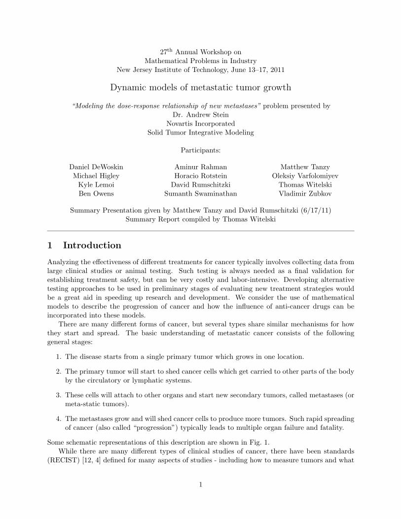
Some schematic representations of this description are shown in Fig. 1.While there are many different types of clinical studies of cancer, there have been standards

(RECIST) [12, 4] defined for many aspects of studies - including how to measure tumors and what

1

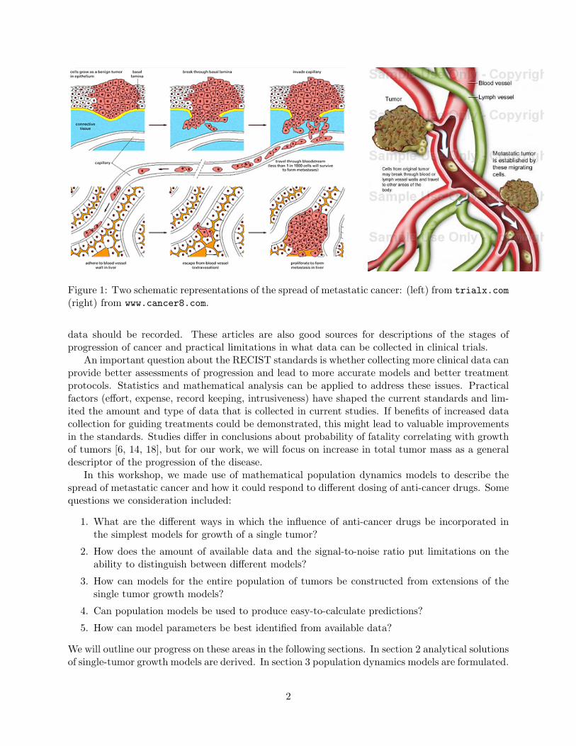
Figure 1: Two schematic representations of the spread of metastatic cancer: (left) from trialx.com(right) from www.cancer8.com.

data should be recorded. These articles are also good sources for descriptions of the stages ofprogression of cancer and practical limitations in what data can be collected in clinical trials.

An important question about the RECIST standards is whether collecting more clinical data canprovide better assessments of progression and lead to more accurate models and better treatmentprotocols. Statistics and mathematical analysis can be applied to address these issues. Practicalfactors (effort, expense, record keeping, intrusiveness) have shaped the current standards and lim-ited the amount and type of data that is collected in current studies. If benefits of increased datacollection for guiding treatments could be demonstrated, this might lead to valuable improvementsin the standards. Studies differ in conclusions about probability of fatality correlating with growthof tumors [6, 14, 18], but for our work, we will focus on increase in total tumor mass as a generaldescriptor of the progression of the disease.

In this workshop, we made use of mathematical population dynamics models to describe thespread of metastatic cancer and how it could respond to different dosing of anti-cancer drugs. Somequestions we consideration included:

1. What are the different ways in which the influence of anti-cancer drugs be incorporated inthe simplest models for growth of a single tumor?

2. How does the amount of available data and the signal-to-noise ratio put limitations on theability to distinguish between different models?

3. How can models for the entire population of tumors be constructed from extensions of thesingle tumor growth models?

4. Can population models be used to produce easy-to-calculate predictions?

5. How can model parameters be best identified from available data?

We will outline our progress on these areas in the following sections. In section 2 analytical solutionsof single-tumor growth models are derived. In section 3 population dynamics models are formulated.

2

In section 4 numerical and analytical approaches for studying the population dynamics systems arepresented. Finally, in section 5 we briefly describe ideas for parameter estimation in models anddirections for further study.

2 Single Tumor Growth ODE Models

The simplest models for growth of a single tumor prescribe a growth rate law as a function of timefor the size of the tumor x(t),

dx

dt= g(x,E), (1)

where E = E(t) is a measure of the effect of anti-cancer drugs being tested. The measure ofthe tumor size as a function of time, x(t), could be given by the volume, radius, or number ofconstituent cells. Since all of these are directly correlated qualitative dynamics will be the sameusing any of these, but typical data will report tumor diameter. The initial size will be writtenas x(0) = x0. For an initial period of time, taken to be the normalized period 0 ≤ t < 1, we willassume that the tumor grows in an untreated state (i.e. with no drug effects, g = g(x, 0)); for latertimes, we will impose a constant drug dose. The influence of drug effects will be modeled as thestep function,

E(t) ≡

{0 0 ≤ t < 1,E∗ t ≥ 1

(2)

where E∗ is a positive constant. The value of E∗ should be correlated with the drug dose, d,but in general will be a function E∗(d), not necessarily just linearly proportional. Often a Hill’sequation (or generalized-Michaelis-Menton or Langmuir model) will be used for the dose-effectrelation [28, 23] in the form

E∗(d) =αdβ

γ + dβ.

Systematic statistical evaluation of dose response models [28, 23, 5, 36] are studied as part ofpharmacology (pharmaco-dynamics).

We considered three models that have closed-form explicit solutions:

1. The linear inhomogeneous (constant growth) model: g(x,E) = k1 − Ex,

dx1

dt= k1 − E1(t)x1, x1(0) = x0, (3a)

x1(t) =

{x0 + k1t 0 ≤ t < 1k1E1

(1− e−E1(t−1)

)+ (x0 + k1)e−E1(t−1) t ≥ 1

(3b)

Untreated, the tumor is predicted to grow linearly with time. When the drug is introduced,depending on the strength of the dose, either the rate of growth is slowed, but not reversed(if E1 < k1/x(1) [the low dose case]), or the tumor will shrink exponentially (if E1 > k1/x(1)[the high dose case]). However in both cases, the predicted long term behavior is for thetumor to reach a finite-size equilibrium state, x∗1 = k1/E1.

2. The logistic growth model: g(x,E) = x(k2 − Ex),

dx2

dt= (k2 − E2(t)x2)x2, x2(0) = x0 (4a)

3

0

0.5

1

0 1 2 3

t

Small noise fitting to single tumor growth

x1(t)x2(t)x3(t)

0

0.5

1

0 1 2 3

t

Medium noise fitting to single tumor growth

x1(t)x2(t)x3(t)

0

0.5

1

0 1 2 3

t

Large noise fitting to single tumor growth

x1(t)x2(t)x3(t)

Figure 2: Best fits of solutions (3b, 4b, 5b) (with optimized model parameters kj , Ej) to simulateddata from (3b) with various levels of additive noise: (left) low noise, with the three models beingclearly distinguishable, (middle) moderate noise, and (right) large amplitude noise.

x2(t) =

{x0e

k2t 0 ≤ t < 1k2x0

E2x0(1−e−k2(t−1))+k2e−k2t t ≥ 1(4b)

Untreated, the tumor under this model exhibits exponential growth. Like the constant growthmodel, whether slowed growth or tumor shrinkage occurs depends on the strength of the drugeffect: E2 ≷ k2/x(1). This model will also lead to a finite-size equilibrium tumor, x∗2 = k2/E2.

3. The linear separable (linear growth) model: g(x,E) = (k3 − E)x,

dx

dt= (k3 − E3(t))x, x3(0) = x0, (5a)

x3(t) =

{x0e

k3t 0 ≤ t < 1x0e

k3+(k3−E3)(t−1) t ≥ 1(5b)

Untreated, the tumor under this model exhibits exponential growth. Strong/weak drug effectsare gaged directly relative to the tumor growth rate, E3 ≷ k3 corresponding to exponentialgrowth/decay of the tumor. For E3 > k3 the tumor will ultimately vanish, x3(t→∞)→ 0.

In all three models, once treatment is started, monotone growth or decay of the tumor is predicted.A generalization that can be incorporated into any of these models is the effect of the tumor

developing resistance to the drug. A simple model for this is an exponential damping factor on thedrug effect, i.e. g = g(x,E(t)e−r(t−1)) with r > 0. These are sometimes called Gompertz models;we were not able to obtain any closed-form solutions for such models.

2.1 Fitting Data to Single Tumor Growth ODE Models

The simple growth models are heuristic and do not attempt to describe the complicated physio-logical processes that govern tumor growth. Consequently, none of the models can be expected toperfectly match any real tumor data, but some models may be better approximations than others.A very basic approach to assessing this can be done by taking a time series of tumor data, {ti, xi}for i = 0, 1, 2, · · · , n can be fit to one of the solution forms (3b, 4b, 5b) using least-squares orsimilar fitting algorithms to determine approximate model parameters, kj , Ej (j = 1, 2, or 3). Themagnitude of the residual error between the data and the optimal-fit solution would give a measureof the goodness-of-fit of the model.

Real tumor data was not available to us, so instead we fitted simulated data (which was producedby solution (3b) with Gaussian noise added) against the three models, see Figure 2. When the level

4

0.001

0.01

0.1

1

1 10 100

std

.dev.

in fi

ttin

g

number of data pts

Small noise fitting to single tumor growth

x1 fitx2 fitx3 fit

0.01

0.1

1

1 10 100

std

.dev.

in fi

ttin

g

number of data pts

Medium noise fitting to single tumor growth

x1 fitx2 fitx3 fit

0.1

1

10

100

1000

1 10 100

std

.dev.

in fi

ttin

g

number of data pts

Large noise fitting to single tumor growth

x1 fitx2 fitx3 fit

Figure 3: Measures of the error in fitting the models (3b, 4b, 5b) against the simulated data fordifferent noise levels and with respect to reduced data sets.

of noise in the data was small, the best-fitting model is easy to identify. For moderate to noisierdata, the difference between the three models can fall within the error bars of the data and then twodifferent models (in this case, the true solution x1(t), and x2(t)) may yield comparable estimates,see Figure 3. For sufficiently large data sets, fitting gives robust results, for very sparse data,parameter estimation and choice of models can be much less reliable.

3 Population dynamics models

A more global and comprehensive description of the progression of cancer in a patient shouldconsider the growth of all of the tumors that are present. We considered two forms of mathematicalpopulation dynamics models. These are equations that describe the evolution of a distributionfunction that gives the number of tumors, n, of each given size, x at time t. If size is treated asa continuous variable, the model is partial differential equation called a “Lotka-McKendrick” or“McKendrick-von Foerster” model. If size is discretized, as in counting the number of cells (or in thecase of polymer chemistry, counting monomer building blocks), then a coupled system of ordinarydifferential equations, sometimes called Becker-Doering equations [13], is produced (sometimes alsocalled polymerization or coagulation/fragmentation models).

These models provide well-defined mathematical frameworks which could be used for matchingagainst data from experiments, clinical studies or simulations [35, 37, 10, 7, 17, 22, 25].

We mention that other studies have also made use of probabilistic models for transitions intumor states (sizes)

P (sj → sj + ∆s) tumor growth P (sj → sj −∆s) tumor shrinkage

and made use of Markov birth/death processes, branching processes, and Poisson process [3, 16,15, 38, 21, 26] but we will not pursue these approaches here.

3.1 A McKendrick-von Foerster population model

Following the work of Iwata et al [19], consider a density function for metastatic tumors of size x asρ = ρ(x, t) where x ≥ 1 is a continuous variable representing tumor size being of one cell or larger.The total number of tumors is given by

N(t) =∫ ∞

1ρ(x, t) dx, (6)

5

and the total tumor mass is the first moment of this distribution,

M(t) =∫ ∞

1xρ(x, t) dx (7)

The density function will evolve according to a conservation law for the number of tumors,

∂ρ

∂t+

∂

∂x(g(x)ρ) = 0, (8a)

where g(x) gives the growth rate for tumors of size x. We assume that initially there no metastases(only a primary tumor of size xp(t)), yielding the initial condition

ρ(x, 0) = 0 1 ≤ x < xp(0). (8b)

The formation or “birth” of metastases comes about from shedding of cells from the primary tumor(and other subsequent tumors) according to a size-dependent birth-rate function β(x). This willgenerate a flux of new tumors into (8a) starting from size x = 1, this is given by the boundarycondition,

g(1)ρ(1, t) =∫ ∞

1β(x)ρ(x, t)dx+ β(xp(t)) (8c)

If β(x) and g(x) are given, then these equations, supplemented by the growth law for the primarytumor,

dxpdt

= g(xp) xp(0) = xp0 (8d)

give a complete problem statement for the population system. This system has been studied asmodel for metastatic cancer in [19, 2, 9], similar mathematical population models have been studiedextensively in context with demographics, ecology, and epidemiology [8, 1, 29, 32, 31, 33, 30, 11].

Equation (8a) is called a size-structured population model. It allows for descriptions of theoverall dynamics of a population whose individual members can range in sizes and may havedifferent size-dependent properties. These models differ from similar-looking but simpler “age-structured” population models (in which x represents the age of each individual member) in thatage increases at an unchangeable rate, dx/dt ≡ 1, whereas size can increase or decrease with timedepending on the form of g(x), as in (8d). Further details of the approach to the analysis of thismodel (method of characteristics) will be detailed below, but it represents a convenient and usefulcondensed form for the study of many (mostly) independent growing tumors, building on the singleODE model given by (1).

3.2 A Becker-Doering-type population balance model

Another related approach seeks to more carefully describe the processes involved in tumor growthor decay. Consider tumor sizes to be discretized, being counted in terms of number of cells present,j = 1, 2, 3, · · · . Let nj be the number of tumors present with j cells. To relate to the model in(8a)), if x represents number of cells, then

nj(t) ∼∫ j+1

jρ(x, t) dx

for more macroscopic scales of measure for x, we can interpret nj(t) ∼ ρ(xj , t)∆x.

6

Then, a linear growth model, extending (5a), with growth rate k1 describing tumors with (j−1)cells growing to join the nj population is

dnj(t)dt

= k1(nj−1 − nj) + f(t)(nj+1 − nj) j = 2, 3, · · · . (9)

where the second describes tumors with (j + 1) cells being shrunk due to drug (and other) effectsdown into the nj population with rate f(t). The above equation applies to all tumors with morethan one cell; the equation for j = 1 takes a special form to incorporate the new single-celledmetastatic tumors shed by all of the larger tumors,

dn1(t)dt

= −k1n1 + f(t)(n2 − n1) + k0

∞∑j=1

jnj

. (10)

The final term in (10) can be related to the boundary condition on new tumors, (8c), with thebirth rate β(x) = k0x mapping onto k0j in the summation over larger tumors.

A rearrangement of the terms in (9) can put it into a form that makes it more clear that itdescribes a system with advection (drift based on the rate k1 − f) and diffusion,

dnjdt

+ [k1 − f(t)](nj+1 − nj) = k1 [(nj+1 − nj)− (nj − nj−1)] , j > 1. (11)

Diffusive effects were neglected in writing (8a). This system of coupled ODEs is closed by distin-guishing equation for the largest tumors,

dnJdt

= k1nJ−1 − f(t)nJ . (12)

The size of the largest tumor, J , itself will increase with time and will be governed by a growthequation analogous to (8d).

4 Results and approaches to solutions

In the following subsections we describe results we obtained on the different models and usingvarious numerical and analytical approaches.

4.1 Numerical simulations of the Becker-Doering model

In a discrete population model, the success of any treatment (which is understood here to increasethe death rate of the cancer cells) will depend on the birth and growth rates of the cancer cells.To view this effect we model the success rates of treatment in this polymerization model with aRECIST-inspired criteria.

We begin by normalizing k0, f, k1 by f , and t by 1/f . I.e. we set f = 1 in all simulations andinterpret t, k0 and k1 accordingly. We begin a simulation by setting

nj(0) = δ1,j (13)

and allowing nj to evolve with f = 0 until a sufficient number of tumors appear. Time integrationof the model was done computationally in MATLAB using ode45. We established lower bound onthe size of detectable tumors jD and calculating the number of detectable tumors [25, 16, 15] as

CD =∑j≥jD

nj(t). (14)

7

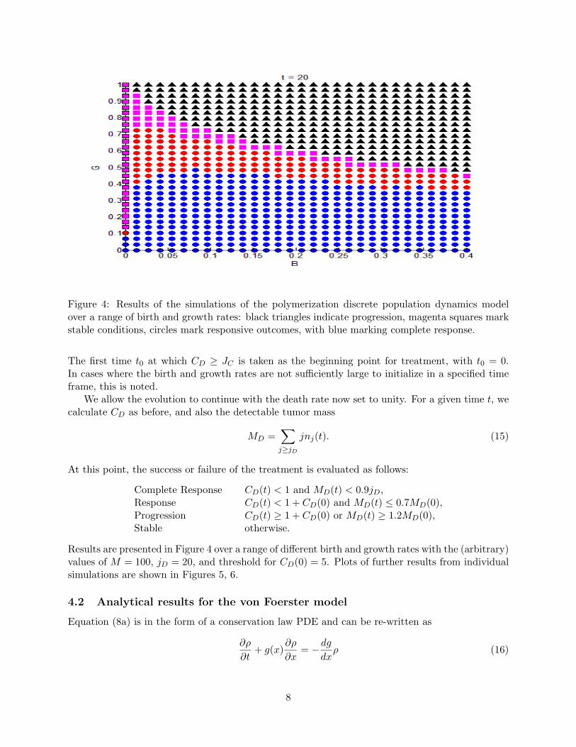
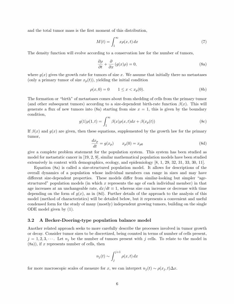
Figure 4: Results of the simulations of the polymerization discrete population dynamics modelover a range of birth and growth rates: black triangles indicate progression, magenta squares markstable conditions, circles mark responsive outcomes, with blue marking complete response.

The first time t0 at which CD ≥ JC is taken as the beginning point for treatment, with t0 = 0.In cases where the birth and growth rates are not sufficiently large to initialize in a specified timeframe, this is noted.

We allow the evolution to continue with the death rate now set to unity. For a given time t, wecalculate CD as before, and also the detectable tumor mass

MD =∑j≥jD

jnj(t). (15)

At this point, the success or failure of the treatment is evaluated as follows:

Complete Response CD(t) < 1 and MD(t) < 0.9jD,Response CD(t) < 1 + CD(0) and MD(t) ≤ 0.7MD(0),Progression CD(t) ≥ 1 + CD(0) or MD(t) ≥ 1.2MD(0),Stable otherwise.

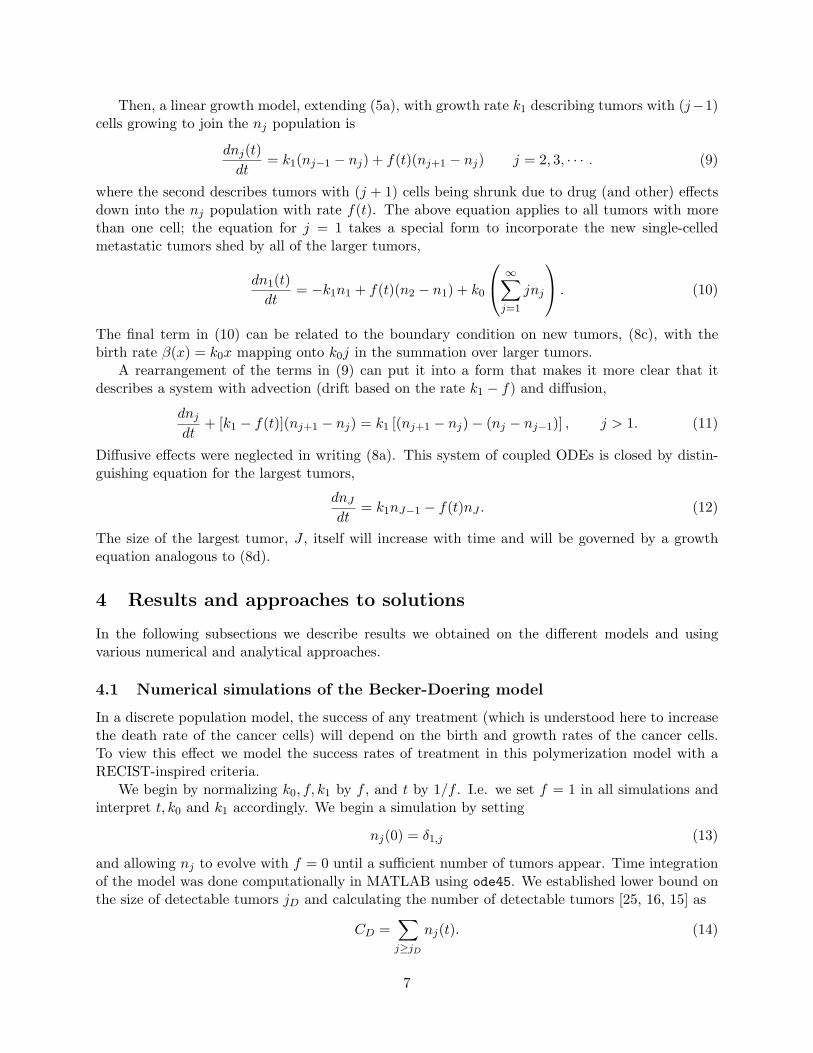
Results are presented in Figure 4 over a range of different birth and growth rates with the (arbitrary)values of M = 100, jD = 20, and threshold for CD(0) = 5. Plots of further results from individualsimulations are shown in Figures 5, 6.

4.2 Analytical results for the von Foerster model

Equation (8a) is in the form of a conservation law PDE and can be re-written as

∂ρ

∂t+ g(x)

∂ρ

∂x= −dg

dxρ (16)

8

Figure 5: Time evolution results from simulations of the discrete population dynamics modelshowing: (left) effective treatment and (right) insufficient treatment and progression of the tumors.

Figure 6: Results from further simulations of the discrete population dynamics model.

9

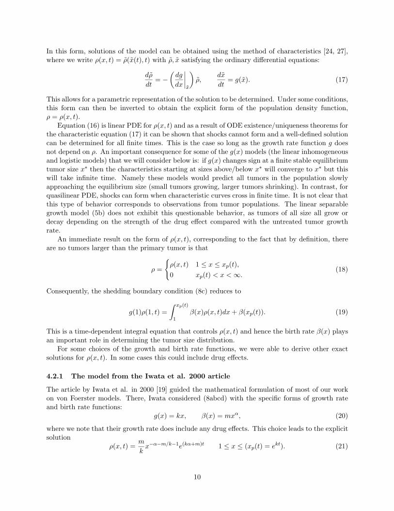
In this form, solutions of the model can be obtained using the method of characteristics [24, 27],where we write ρ(x, t) = ρ(x(t), t) with ρ, x satisfying the ordinary differential equations:

dρ

dt= −

(dg

dx

∣∣∣∣x

)ρ,

dx

dt= g(x). (17)

This allows for a parametric representation of the solution to be determined. Under some conditions,this form can then be inverted to obtain the explicit form of the population density function,ρ = ρ(x, t).

Equation (16) is linear PDE for ρ(x, t) and as a result of ODE existence/uniqueness theorems forthe characteristic equation (17) it can be shown that shocks cannot form and a well-defined solutioncan be determined for all finite times. This is the case so long as the growth rate function g doesnot depend on ρ. An important consequence for some of the g(x) models (the linear inhomogeneousand logistic models) that we will consider below is: if g(x) changes sign at a finite stable equilibriumtumor size x∗ then the characteristics starting at sizes above/below x∗ will converge to x∗ but thiswill take infinite time. Namely these models would predict all tumors in the population slowlyapproaching the equilibrium size (small tumors growing, larger tumors shrinking). In contrast, forquasilinear PDE, shocks can form when characteristic curves cross in finite time. It is not clear thatthis type of behavior corresponds to observations from tumor populations. The linear separablegrowth model (5b) does not exhibit this questionable behavior, as tumors of all size all grow ordecay depending on the strength of the drug effect compared with the untreated tumor growthrate.

An immediate result on the form of ρ(x, t), corresponding to the fact that by definition, thereare no tumors larger than the primary tumor is that

ρ =

{ρ(x, t) 1 ≤ x ≤ xp(t),0 xp(t) < x <∞.

(18)

Consequently, the shedding boundary condition (8c) reduces to

g(1)ρ(1, t) =∫ xp(t)

1β(x)ρ(x, t)dx+ β(xp(t)). (19)

This is a time-dependent integral equation that controls ρ(x, t) and hence the birth rate β(x) playsan important role in determining the tumor size distribution.

For some choices of the growth and birth rate functions, we were able to derive other exactsolutions for ρ(x, t). In some cases this could include drug effects.

4.2.1 The model from the Iwata et al. 2000 article

The article by Iwata et al. in 2000 [19] guided the mathematical formulation of most of our workon von Foerster models. There, Iwata considered (8abcd) with the specific forms of growth rateand birth rate functions:

g(x) = kx, β(x) = mxα, (20)

where we note that their growth rate does include any drug effects. This choice leads to the explicitsolution

ρ(x, t) =m

kx−α−m/k−1e(kα+m)t 1 ≤ x ≤ (xp(t) = ekt). (21)

10

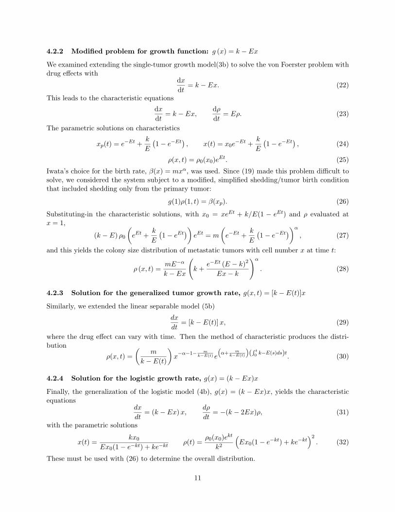
4.2.2 Modified problem for growth function: g (x) = k − Ex

We examined extending the single-tumor growth model(3b) to solve the von Foerster problem withdrug effects with

dxdt

= k − Ex. (22)

This leads to the characteristic equations

dxdt

= k − Ex, dρdt

= Eρ. (23)

The parametric solutions on characteristics

xp(t) = e−Et +k

E

(1− e−Et

), x(t) = x0e

−Et +k

E

(1− e−Et

), (24)

ρ(x, t) = ρ0(x0)eEt. (25)

Iwata’s choice for the birth rate, β(x) = mxα, was used. Since (19) made this problem difficult tosolve, we considered the system subject to a modified, simplified shedding/tumor birth conditionthat included shedding only from the primary tumor:

g(1)ρ(1, t) = β(xp). (26)

Substituting-in the characteristic solutions, with x0 = xeEt + k/E(1 − eEt) and ρ evaluated atx = 1,

(k − E) ρ0

(eEt +

k

E

(1− eEt

))eEt = m

(e−Et +

k

E

(1− e−Et

))α, (27)

and this yields the colony size distribution of metastatic tumors with cell number x at time t:

ρ (x, t) =mE−α

k − Ex

(k +

e−Et (E − k)2

Ex− k

)α. (28)

4.2.3 Solution for the generalized tumor growth rate, g(x, t) = [k − E(t)]x

Similarly, we extended the linear separable model (5b)

dx

dt= [k − E(t)]x, (29)

where the drug effect can vary with time. Then the method of characteristic produces the distri-bution

ρ(x, t) =(

m

k − E(t)

)x−α−1− m

k−E(t) e

“α+ m

k−E(t)

”(R t0 k−E(s)ds)t

. (30)

4.2.4 Solution for the logistic growth rate, g(x) = (k − Ex)x

Finally, the generalization of the logistic model (4b), g(x) = (k − Ex)x, yields the characteristicequations

dx

dt= (k − Ex)x,

dρ

dt= −(k − 2Ex)ρ, (31)

with the parametric solutions

x(t) =kx0

Ex0(1− e−kt) + ke−ktρ(t) =

ρ0(x0)ekt

k2

(Ex0(1− e−kt) + ke−kt

)2. (32)

These must be used with (26) to determine the overall distribution.

11

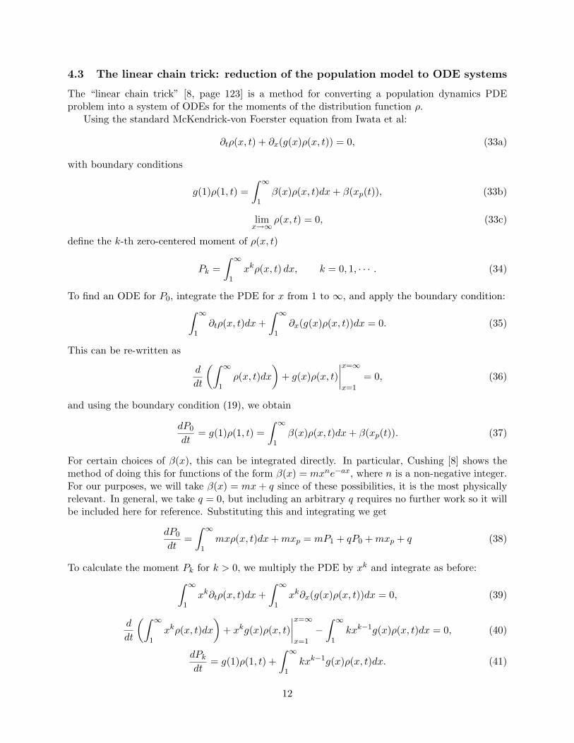
4.3 The linear chain trick: reduction of the population model to ODE systems

The “linear chain trick” [8, page 123] is a method for converting a population dynamics PDEproblem into a system of ODEs for the moments of the distribution function ρ.

Using the standard McKendrick-von Foerster equation from Iwata et al:

∂tρ(x, t) + ∂x(g(x)ρ(x, t)) = 0, (33a)

with boundary conditions

g(1)ρ(1, t) =∫ ∞

1β(x)ρ(x, t)dx+ β(xp(t)), (33b)

limx→∞

ρ(x, t) = 0, (33c)

define the k-th zero-centered moment of ρ(x, t)

Pk =∫ ∞

1xkρ(x, t) dx, k = 0, 1, · · · . (34)

To find an ODE for P0, integrate the PDE for x from 1 to ∞, and apply the boundary condition:∫ ∞1

∂tρ(x, t)dx+∫ ∞

1∂x(g(x)ρ(x, t))dx = 0. (35)

This can be re-written as

d

dt

(∫ ∞1

ρ(x, t)dx)

+ g(x)ρ(x, t)∣∣∣∣x=∞x=1

= 0, (36)

and using the boundary condition (19), we obtain

dP0

dt= g(1)ρ(1, t) =

∫ ∞1

β(x)ρ(x, t)dx+ β(xp(t)). (37)

For certain choices of β(x), this can be integrated directly. In particular, Cushing [8] shows themethod of doing this for functions of the form β(x) = mxne−ax, where n is a non-negative integer.For our purposes, we will take β(x) = mx+ q since of these possibilities, it is the most physicallyrelevant. In general, we take q = 0, but including an arbitrary q requires no further work so it willbe included here for reference. Substituting this and integrating we get

dP0

dt=∫ ∞

1mxρ(x, t)dx+mxp = mP1 + qP0 +mxp + q (38)

To calculate the moment Pk for k > 0, we multiply the PDE by xk and integrate as before:∫ ∞1

xk∂tρ(x, t)dx+∫ ∞

1xk∂x(g(x)ρ(x, t))dx = 0, (39)

d

dt

(∫ ∞1

xkρ(x, t)dx)

+ xkg(x)ρ(x, t)∣∣∣∣x=∞x=1

−∫ ∞

1kxk−1g(x)ρ(x, t)dx = 0, (40)

dPkdt

= g(1)ρ(1, t) +∫ ∞

1kxk−1g(x)ρ(x, t)dx. (41)

12

Figure 7: Evolution of the moments of ρ(x, t) using the moment model (42).

The choice of g(x) is important. In the simplest case of a linear growth function, g(x) = ax+ b,we can proceed analytically:

dPkdt

= g(1)ρ(1, t) +∫ ∞

1kxk−1(ax+ b)ρ(x, t)dx, (42)

= mP1 + qP0 +mxp + q +∫ ∞

1kxk−1(ax+ b)ρ(x, t)dx,

= mP1 + qP0 +mxp + q + akPk + bkPk−1.

Thus, in this case, we have a closed system of ODEs for any set of moments of ρ: P0, . . . , Pn, withn ≥ 1. It is important to note that these are not the mean centered moments. However, theydo give important information, such as the total number of metastases (P0), the total number oftumor cells (P1), and the mean number of cells per tumor (P1/P0). In addition, there are numericalmethods of reconstructing a density function from a finite set of its moments [20]. This would bean easy way of gaining more information about the size density function without solving the fullPDE. An example plot of the zeroth through fourth moments of ρ is given below for g(x) = ax,β(x) = mx with a = 0.0286 day−1 and m = 5.3 × 10−7 (cell day)−1, see Figure 7. After 60 days,there are approximately 53 metastases present and 901 total tumor cells, for an average of about17 cells per tumor.

A second reasonable growth function we worked with was logistic growth, g(x) = x(ax + b).Solving for the ODE for Pk yields:

dPkdt

= g(1)ρ(1, t) +∫ ∞

1kxk−1x(ax+ b)ρ(x, t)dx (43)

= mP1 + qP0 +mxp + q +∫ ∞

1kxk(ax+ b)ρ(x, t)dx

= mP1 + qP0 +mxp + q + akPk+1 + bkPk

In this case, the system is not closed, and some further assumptions would need to be made inorder to proceed. This is a significant limitation of the method, and similar problems are found

13

with other growth and shedding functions. It would be interesting to examine this method furtherto look for any possible extensions that could be of use.

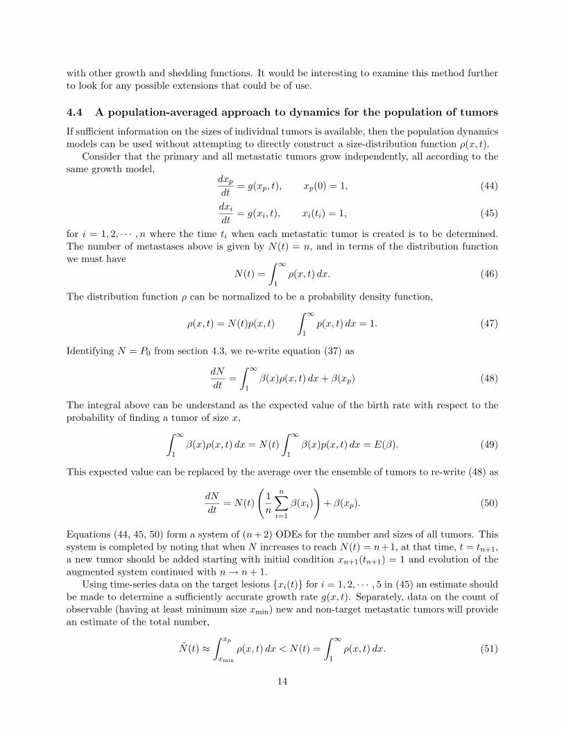
4.4 A population-averaged approach to dynamics for the population of tumors

If sufficient information on the sizes of individual tumors is available, then the population dynamicsmodels can be used without attempting to directly construct a size-distribution function ρ(x, t).

Consider that the primary and all metastatic tumors grow independently, all according to thesame growth model,

dxpdt

= g(xp, t), xp(0) = 1, (44)

dxidt

= g(xi, t), xi(ti) = 1, (45)

for i = 1, 2, · · · , n where the time ti when each metastatic tumor is created is to be determined.The number of metastases above is given by N(t) = n, and in terms of the distribution functionwe must have

N(t) =∫ ∞

1ρ(x, t) dx. (46)

The distribution function ρ can be normalized to be a probability density function,

ρ(x, t) = N(t)p(x, t)∫ ∞

1p(x, t) dx = 1. (47)

Identifying N = P0 from section 4.3, we re-write equation (37) as

dN

dt=∫ ∞

1β(x)ρ(x, t) dx+ β(xp) (48)

The integral above can be understand as the expected value of the birth rate with respect to theprobability of finding a tumor of size x,∫ ∞

1β(x)ρ(x, t) dx = N(t)

∫ ∞1

β(x)p(x, t) dx = E(β). (49)

This expected value can be replaced by the average over the ensemble of tumors to re-write (48) as

dN

dt= N(t)

(1n

n∑i=1

β(xi)

)+ β(xp). (50)

Equations (44, 45, 50) form a system of (n+ 2) ODEs for the number and sizes of all tumors. Thissystem is completed by noting that when N increases to reach N(t) = n+1, at that time, t = tn+1,a new tumor should be added starting with initial condition xn+1(tn+1) = 1 and evolution of theaugmented system continued with n→ n+ 1.

Using time-series data on the target lesions {xi(t)} for i = 1, 2, · · · , 5 in (45) an estimate shouldbe made to determine a sufficiently accurate growth rate g(x, t). Separately, data on the count ofobservable (having at least minimum size xmin) new and non-target metastatic tumors will providean estimate of the total number,

N(t) ≈∫ xp

xmin

ρ(x, t) dx < N(t) =∫ ∞

1ρ(x, t) dx. (51)

14

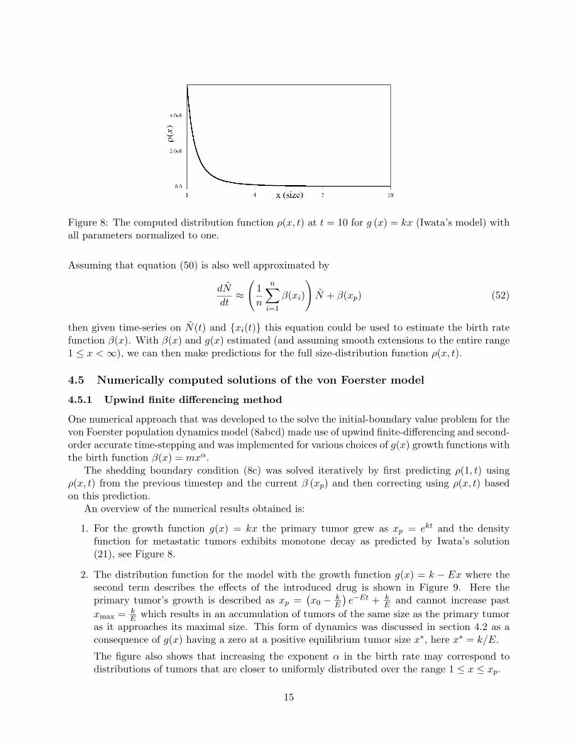
Figure 8: The computed distribution function ρ(x, t) at t = 10 for g (x) = kx (Iwata’s model) withall parameters normalized to one.

Assuming that equation (50) is also well approximated by

dN

dt≈

(1n

n∑i=1

β(xi)

)N + β(xp) (52)

then given time-series on N(t) and {xi(t)} this equation could be used to estimate the birth ratefunction β(x). With β(x) and g(x) estimated (and assuming smooth extensions to the entire range1 ≤ x <∞), we can then make predictions for the full size-distribution function ρ(x, t).

4.5 Numerically computed solutions of the von Foerster model

4.5.1 Upwind finite differencing method

One numerical approach that was developed to the solve the initial-boundary value problem for thevon Foerster population dynamics model (8abcd) made use of upwind finite-differencing and second-order accurate time-stepping and was implemented for various choices of g(x) growth functions withthe birth function β(x) = mxα.

The shedding boundary condition (8c) was solved iteratively by first predicting ρ(1, t) usingρ(x, t) from the previous timestep and the current β (xp) and then correcting using ρ(x, t) basedon this prediction.

An overview of the numerical results obtained is:

1. For the growth function g(x) = kx the primary tumor grew as xp = ekt and the densityfunction for metastatic tumors exhibits monotone decay as predicted by Iwata’s solution(21), see Figure 8.

2. The distribution function for the model with the growth function g(x) = k − Ex where thesecond term describes the effects of the introduced drug is shown in Figure 9. Here theprimary tumor’s growth is described as xp =

(x0 − k

E

)e−Et + k

E and cannot increase pastxmax = k

E which results in an accumulation of tumors of the same size as the primary tumoras it approaches its maximal size. This form of dynamics was discussed in section 4.2 as aconsequence of g(x) having a zero at a positive equilibrium tumor size x∗, here x∗ = k/E.

The figure also shows that increasing the exponent α in the birth rate may correspond todistributions of tumors that are closer to uniformly distributed over the range 1 ≤ x ≤ xp.

15

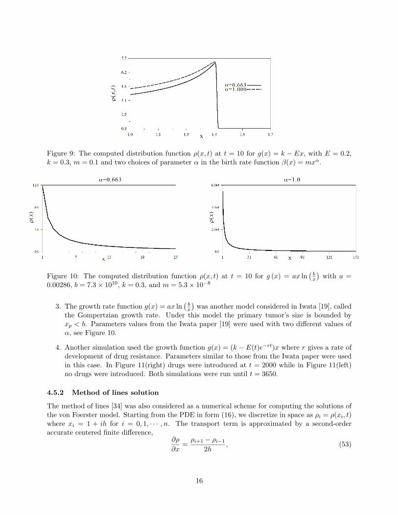
Figure 9: The computed distribution function ρ(x, t) at t = 10 for g(x) = k − Ex, with E = 0.2,k = 0.3, m = 0.1 and two choices of parameter α in the birth rate function β(x) = mxα.

Figure 10: The computed distribution function ρ(x, t) at t = 10 for g (x) = ax ln(bx

)with a =

0.00286, b = 7.3× 1010, k = 0.3, and m = 5.3× 10−8

3. The growth rate function g(x) = ax ln(bx

)was another model considered in Iwata [19], called

the Gompertzian growth rate. Under this model the primary tumor’s size is bounded byxp < b. Parameters values from the Iwata paper [19] were used with two different values ofα, see Figure 10.

4. Another simulation used the growth function g(x) = (k − E(t)e−rt)x where r gives a rate ofdevelopment of drug resistance. Parameters similar to those from the Iwata paper were usedin this case. In Figure 11(right) drugs were introduced at t = 2000 while in Figure 11(left)no drugs were introduced. Both simulations were run until t = 3650.

4.5.2 Method of lines solution

The method of lines [34] was also considered as a numerical scheme for computing the solutions ofthe von Foerster model. Starting from the PDE in form (16), we discretize in space as ρi = ρ(xi, t)where xi = 1 + ih for i = 0, 1, · · · , n. The transport term is approximated by a second-orderaccurate centered finite difference,

∂ρ

∂x=ρi+1 − ρi−1

2h, (53)

16

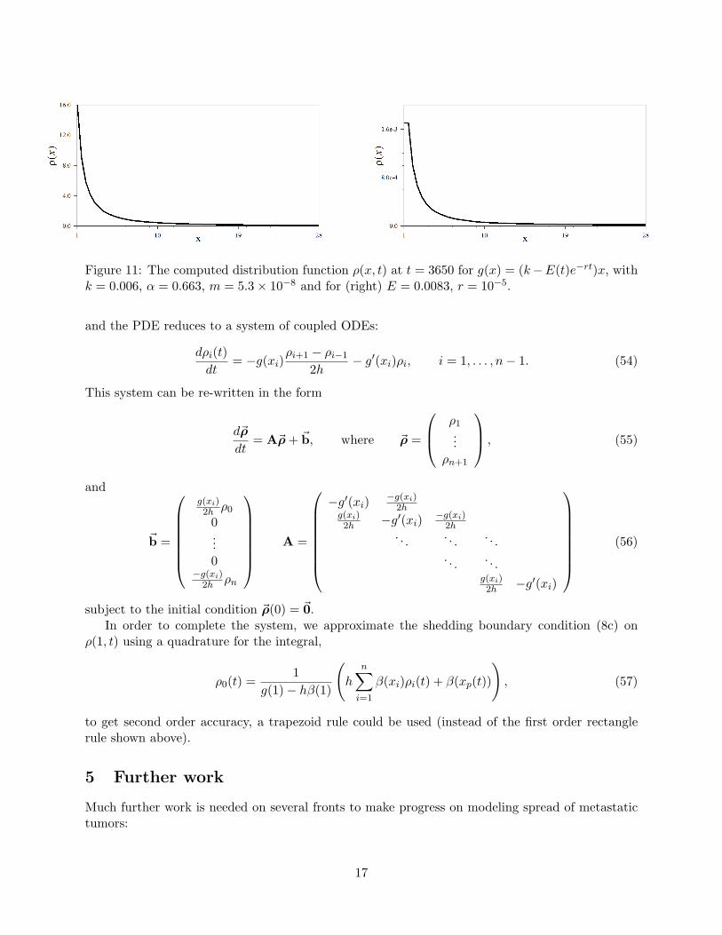
Figure 11: The computed distribution function ρ(x, t) at t = 3650 for g(x) = (k−E(t)e−rt)x, withk = 0.006, α = 0.663, m = 5.3× 10−8 and for (right) E = 0.0083, r = 10−5.

and the PDE reduces to a system of coupled ODEs:

dρi(t)dt

= −g(xi)ρi+1 − ρi−1

2h− g′(xi)ρi, i = 1, . . . , n− 1. (54)

This system can be re-written in the form

d~ρ

dt= A~ρ + ~b, where ~ρ =

ρ1...

ρn+1

, (55)

and

~b =

g(xi)2h ρ0

0...0

−g(xi)2h ρn

A =

−g′(xi) −g(xi)2h

g(xi)2h −g′(xi) −g(xi)

2h. . . . . . . . .

. . . . . .g(xi)2h −g′(xi)

(56)

subject to the initial condition ~ρ(0) = ~0.In order to complete the system, we approximate the shedding boundary condition (8c) on

ρ(1, t) using a quadrature for the integral,

ρ0(t) =1

g(1)− hβ(1)

(h

n∑i=1

β(xi)ρi(t) + β(xp(t))

), (57)

to get second order accuracy, a trapezoid rule could be used (instead of the first order rectanglerule shown above).

5 Further work

Much further work is needed on several fronts to make progress on modeling spread of metastatictumors:

17

1. Fitting data to models, parameter estimation for multiple tumor time series and multiplepatient data requires more careful statistical analysis to form a detailed understanding of theconfidence level that can be attributed to predictions from the models.

2. Incorporating limitations and uncertainties in the measurable clinical data into the aboveanalysis. Also exploration is needed in whether good inferences for these models be drawnfrom more limited qualitative clinical data.

3. Comparing the analytical and computed results from the PDE, discrete population and poly-merization models to determine which approaches provide the most robust predictions at anacceptable level of computational workload.

References

[1] J. Banasiak and W. Lamb. Coagulation, fragmentation and growth processes in a size struc-tured population. Discrete and Continuous Dynamical Systems, Series B, 11(3):563–585, 2009.

[2] D. Barbolosi, A. Benabdallah, F. Hubert, and F. Verga. Mathematical and numerical analysisfor a model of growing metastatic tumors. Mathematical Biosciences, 218:1–14, 2009.

[3] R. Bartoszynski, L. Edler, L. Hanin, A. Kopp-Schneider, L. Pavlova, A. Tsodikov, A. Zorin,and A.Y. Yakovlev. Modeling cancer detection: tumor size as a source of information onunobservable stages of carcinogenesis. Mathematical Biosciences, 171:113–142, 2001.

[4] J. Bogaerts, R. Ford, D. Sargent, L. H. Schwartz, L. Rubinstein, D. Lacombe, E. Eisenhauer,J. Verweij, and P. Therasse. Individual patient data analysis to assess modifications to theRECIST criteria. European Journal of Cancer, 45:248–260, 2009.

[5] P. L. Bonate. Modeling tumor growth in oncology. In P.L. Bonate and D.R. Howard, editors,Pharmacokinetics in Drug Development, volume 3, pages 1–19. Springer Verlag, New York,2011.

[6] R. Bruno and L. Claret. On the use of change in tumor size to predict survival in clinicaloncology studies: Toward a new paradigm to design and evaluate phase II studies. Clinicalpharmacology and Therapeutics, 86(2):136–138, 2009.

[7] L. Claret, P. Girard, P. M. Hoff, E. van Cutsem, K. P. Zuideveld, K. Jorga, J. Fagerberg, andR. Bruno. Model-based prediction of phase III overall survival in colorectal cancer on the basisof phase II tumor dynamics. J. Clinical Oncology, 27:1–7, 2009.

[8] J. M. Cushing. An introduction to structured population dynamics, volume 71 of CBMS-NSF Regional Conference Series in Applied Mathematics. Society for Industrial and AppliedMathematics (SIAM), Philadelphia, PA, 1998.

[9] A. Devys, T. Goudon, and P. Lafitte. A model describing the growth and the size distribution ofmultiple metastatic tumors. Discrete and Continuous Dynamical Systems, Series B, 12(4):731–767, 2009.

[10] J. R. S. Douglas. Significance of the size distribution of bloodborne metastases. Cancer,27:379–390, 1971.

18

[11] M. Doumic, B. Perthame, and J. P. Zubelli. Numerical solution of an inverse problem insize-structured population dynamics. Inverse Problems, 25(045008):1–25, 2009.

[12] E. A. Eisenhauer, P. Therasse, J. Bogaerts, L. H. Schwartz, R. Ford, J. Dancey, S. Arbuckh,S. Gwyther, M. Mooney, L. Rubinsteing, L. Shankar, L. Dodd, R. Kaplan, D. Lacombe, andJ. Verweij. New response evaluation criteria in solid tumours: Revised RECIST guideline(version 1.1). European Journal of Cancer, 45:228–247, 2009.

[13] J. A. Fozard and J. R. King. Population-scale modelling of cellular chemotaxis and aggregation.IMA journal of applied mathematics, 73:69–106, 2008.

[14] J. Fridlyand, L. D. Kaiser, and G. Fyfe. Analysis of tumor burden versus progression-freesurvival for phase II decision making. Contemporary Clinical Trials, 32:446–452, 2011.

[15] L. Hanin and O. Korosteleva. Does extirpation of the primary breast tumor give boost togrowth of metastases? evidence revealed by mathematical modeling. Mathematical Bio-sciences, 223:133–141, 2010.

[16] L. Hanin, J. Rose, and M. Zaider. A stochastic model for the sizes of detectable metastases.Journal of Theoretical Biology, 243:407–417, 2006.

[17] D. Hart, E. Shochart, and Z. Agur. The growth law of primary breast cancer as inferred frommammography screening trials data. British Journal of Cancer, 78(3):382–387, 1998.

[18] B. E. Houk, C. L. Bello, B. Poland, L. S. Rosen, G. D. Demetri, and R. J. Motzer. Rela-tionship between exposure to sunitinib and efficacy and tolerability endpoints in patients withcancer: results of a pharmacokinetic/pharmacodynamic meta-analysis. Cancer Chemother.Pharmacol., 66:357–371, 2010.

[19] K. Iwata, K. Kawasaki, and N. Shigesada. A dynamical model for the growth and size distri-bution of multiple metastatic tumors. Journal of Theoretical Biology, 203:177–186, 2000.

[20] V. John, I. Angelov, A. A. Oencuel, and D. Thevenin. Techniques for the reconstruction of adistribution from a finite number of its moments. Chemical Engineering Science, 62(11):2890–2904, 2007.

[21] W. S. Kendal. The size distribution of human hematogenous metastases. Journal of TheoreticalBiology, 211:29–38, 2001.

[22] S. P. Lee, J.-R. Sun, H. Qian, W. H. McBride, and H. R. Withers. Characterization ofmetastatic tumor formation by the colony size distribution. arXiv, q-bio/0608024:1–14, 2006.

[23] P. Lees, F. M. Cunningham, and J. Elliott. Principles of pharmacodynamics and their appli-cations in veterinary pharmacology. J. vet. pharmacol. therap., 27:397–414, 2004.

[24] J. D. Logan. Applied Mathematics, 3rd edition. Wiley-Interscience, New York, 2006.

[25] G.B.A. Lorentz, G.H. Alphons, R. Goei, and J.M.A. van Engelshoven. Miss rate of lung canceron the chest radiograph in clinical practice. Chest, 115:720–724, 1999.

[26] P. L. Meyer. Introductory probability and statistical applications, 2nd ed. Addision-Wesley,New York, 1970.

19

[27] J. Ockendon, S. Howison, A. Lacey, and A. Movchan. Applied partial differential equations.Oxford University Press, Oxford, revised edition, 2003.

[28] International Programme on Chemical Safety, editor. Principles of modeling dose-response forthe reisk assessement of chemicals. World Health Organization, Environmental Health Criteria239, Geneva, Switzerland, 2009.

[29] B. Perthame. Transport equations in biology. Frontiers in Mathematics. Birkhauser Verlag,Basel, 2007.

[30] B. Perthame and J. P. Zubelli. On the inverse problem for a size-structured population model.Inverse Problems, 23:1037–1052, 2007.

[31] M. Plant and W. Rundell. Determining a coefficient in a first-order hyperbolic equation. SIAMJ. Appl. Math., 51(2):494–506, 1991.

[32] W. Rundell. Determining the birth function an age structured population. MathematicalPopulation Studies, 1(4):377–395, 1989.

[33] W. Rundell. Determining the death rate for an age-structured population from census data.SIAM J. Appl. Math., 53(6):1731–1746, 1993.

[34] W. E. Schiesser. The Numerical Method of Lines: Integration of Partial Differential Equations.Academic Press, San Diego, 1991.

[35] A. Stein, W.-P. Wang, A. Carter, O. Chiparus, N. Hollaender, H. Kim, R. Motzer, and C. Sarr.Dynamic tumor modeling of the RECORD-1 phase 3 trial of everolimus quantifies relationshipbetween dose and tumor growth in metastatic renal cell carcinoma. Presented at the 26th An-nual European Association of Urology (EAU) Congress; 18 - 22 March 2011; Vienna, Austria,2011.

[36] L.-S. Tham, L.-Z. Wang, R. A. Soo, S.-C. Lee, H.-S. Lee, W.-P. Yong, B.-C. Goh, and N. H.G.Holford. A pharmacodynamic model for the time course of tumor shrinkage by gemcitabineand carboplatin in non-small cell lung cancer patients. Clin. Cancer Res., 14(13):4213–4218,2008.

[37] Y. Wang, C. Sung, C. Dartois, R. Ramchandani, B. P. Booth, E. Rock, and J. Gobburu.Elucidation of relationship between tumor size and survival in non-small-cell lung cancer pa-tients can aid early decision making in clinical drug development. Clinical pharmacology andTherapeutics, 86(2):167–174, 2009.

[38] M. Zaider and L. Hanin. Tumor control probability in radiation treatment. Medical Physics,38(2):574–583, 2011.

20