NOTICE - Portland State Universityweb.pdx.edu/~mcclured/Stat Mech/Computer Rounding Error...There...

NOTICE

The following two chapters are copyrighted to Professor David McClure at Portland State University, Chemistry and Physics Departments, all rights reserved. These chapters first appeared in the text “Computational Physics Guide”, D. Al. IORDACHE, Fl. POP and C. ROSU, Editors; Copyright ©, 2009, Editura, Politehnica Press. ISBN: 978-606-515-062-1 and 978-606-515-063-8. No part of this publication may be reproduced, stored, in or introduced into a retrieval system, or transmitted, in any form, or by any means (electronic, mechanical, photocopying, recording, or otherwise), without the prior written permission of the copyright owner. Professor McClure can be reached at: [email protected]

mailto:[email protected]�

COMPUTATIONAL PHYSICS LABORATORY GUIDE 2

9. COMPUTER ROUNDING ERRORS: BASICS

It is a given that measurement errors, both systematic and random, are always associated with experimental data. Obviously then, it is incumbent upon the investigator to design the experiment with this fact in mind so that these errors can be realistically estimated for each variable measured. What is not always appreciated, however, is that these experimental errors do not form a complete set because of the data reduction process.

By “data reduction” we mean the totality of steps that go into the manipulation of the experimental raw data in order to arrive at the final results. This notion is not limited to experimental data either; it applies just as well to any theoretical analysis where numerical approximations are made along the way.

The byproduct of this data reduction process is that every level of approximation will contribute additional degrees of uncertainty to the results. If these computations also happen to involve the use of a computer, then an additional error, which is called ‘computer round off’ or rounding error, and is a result of the digitizing process itself, can result for reasons that are the subject of this chapter.

The following examples should give a feel for the importance of this topic. 9.1. EXAMPLES OF COMPUTER ERROR

There are a number of cases of computer rounding errors with serious consequences that one might cite [Vui], [Huk09]. For example, the failure of the European space Agency’s Ariane 5 rocket which self-destructed 37 seconds after launch when a program tried to represent a 64 bit double precision floating point number as a 16 bit short integer. Overflow occurred which shut down the guidance system leading to self-destruction. [Lio]

Another classic case of rounding error occurred when, during the Gulf War in 1991, a Patriot Missile failed to stop a Scud Missile resulting in

Computer Rounding Errors 3

28 deaths and injuries to nearly 100. The problem was traced to rounding inconsistencies in the clock, which after 100 hours accumulated a rounding error of 0.3433 seconds. During that interval a Scud missile would travel more than a half-kilometer. [Lum]

EXAMPLE (9.1)

A much more mundane example is the following. When we enter a number into computer memory from the keyboard, we can surely expect the computer to be faithful to our wishes and save the number without error. Or can we? To demonstrate that a problem can sometimes occur, we store a 20-digit number using double precision, recall the number and then print it to obtain:

INPUT: 12345678901234567890 OUTPUT: 12345678901234569000

Now one could certainly argue that an error in the 17th digit is of little consequence, and in a single computation that is generally true. However, in the right circumstances, this seemingly trivial error can propagate and magnify alarmingly as the next example shows.

EXAMPLE (9.2)

Suppose you had occasion to evaluate the following integral,

1

0exp( -1) n

n x x dxI = ∫

for say, the first 50 values of n. One could apply a standard numerical procedure for each integer value of n but the process is tedious at best, and in this case, unnecessary. Instead, repeated by-parts integration will establish the exact recursion relationship: 11 −⋅−= nn InI n = 2, 3,··· which says, if we know a single value of I, say I1, then we can calculate each succeeding value of In without having to do any additional integration. That's the good news. Now for n = 1, the integral (and this is the only actual integration required - also good news) is just a standard form for which I1 =1/e = 0.367879... . From here on it is a simple matter to calculate that


I2 = 0.264241, I3 = 0.207277 and so on until we finally compute that

I50 = -3.78009 x 1047. Both I2 and I3 are correct to at least the number of significant figures given, but, and here's the bad news, the correct value for I50 is actually 0.019238···, a difference which represents an error of ludicrous proportions. The problem, as we shall see, lies entirely with the computer and not with the mathematics.

Our final example illustrates the distinction between round off error and truncation error. By 'truncation error', we mean error which results whenever one uses an approximate operation in a numerical method as a substitute for an exact operation. Examples include using a finite number of terms in summing an infinite series, or using a polynomial to approximate an arbitrary function.

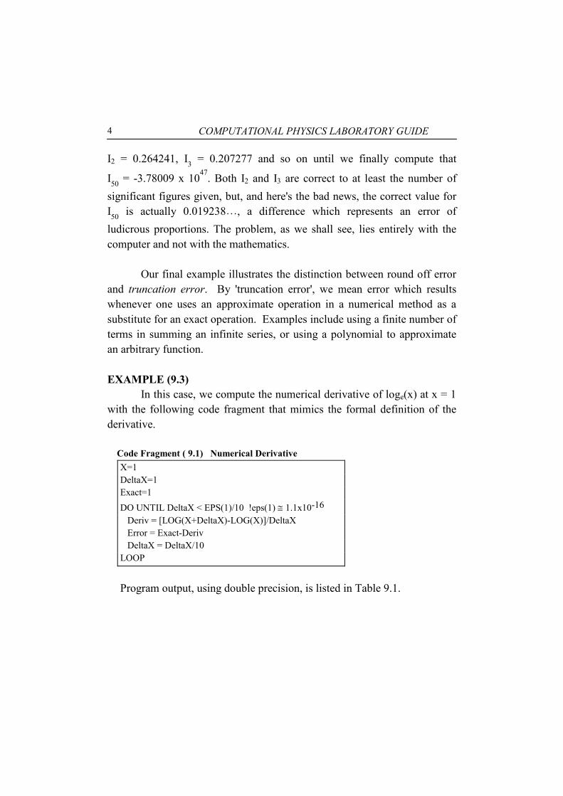
EXAMPLE (9.3)

In this case, we compute the numerical derivative of loge(x) at x = 1 with the following code fragment that mimics the formal definition of the derivative. Code Fragment ( 9.1) Numerical Derivative

X=1 DeltaX=1 Exact=1 DO UNTIL DeltaX < EPS(1)/10 !eps(1) ≅ 1.1x10-16 Deriv = [LOG(X+DeltaX)-LOG(X)]/DeltaX Error = Exact-Deriv DeltaX = DeltaX/10 LOOP

Program output, using double precision, is listed in Table 9.1.


Table (9.1) Rounding vs Truncation Error

We see that truncation error, that is, the error associated with

approximating an infinitesimal with a finite delta x, is very severe at the beginning when delta x is large, but, as one would expect, decreases steadily until we reach a delta x of about 10-8. At this point, round off error takes over and eventually destroys any hope of an accurate numerical derivative.

Figure 9.1 is a plot of the Log[absolute error] on the y axis versus Log[Delta x]| for about a 100 points. Notice how the truncation error decreases in a linear fashion while the round off error increases with a quasi random (but reproducible) component.

Figure (9.1) Log[Absolute Error] vs Log[Delta x]

DELTA X DERIVATIVE ERROR

truncation error dominates 1E+00 0.6931471806 3.07E-01 1E-01 0.9531017980 4.69E-02 1E-02 0.9950330853 4.97E-03 1E-03 0.9995003331 5.00E-04 1E-04 0.9999500033 5.00E-05 1E-05 0.9999950000 5.00E-06 1E-06 0.9999994999 5.00E-07 1E-07 0.9999999506 4.94E-08 1E-08 0.9999999889 1.11E-08 round off error dominates 1E-09 1.0000000822 -0.82E-07 1E-10 1.0000000827 -0.83E-07 1E-11 1.0000000827 -0.83E-07 1E-12 1.0000889006 -0.89E-04 1E-13 0.9992007222 7.99E-04 1E-14 0.9992007222 7.99E-04 1E-15 1.1102230246 -0.11E-00 1E-16 0.0000000000 1.00E-00


These last two examples illustrate just how pernicious round off error can be, especially if the offending block of computer code is producing erroneous output to be used, sight unseen, by other parts of the program. Before we discuss why round off errors occur we should first define the standard method of reckoning computer errors in terms of their absolute and relative values.

9.2. ABSOLUTE AND RELATIVE ERRORS

Absolute Error is defined here as the absolute value of the difference between the exact value of some quantity x (almost always unknown), and its approximate measured value x*, that is:

Absolute Error ≡ AE = |x - x*| (9.1)

If the sign of the absolute error is important, and it often is, then the

absolute value signs are omitted. As an error measure, the absolute error can be rather misleading since it does not take into account the magnitude of x itself. For example, an absolute error of 5 cm is probably acceptable when discussing the circumference of the earth, but would likely represent a disaster if it was the accuracy used to drill a burr hole in brain surgery. The Relative Error overcomes this shortcoming with the definition:

Relative Error ≡ RE = Absolute Error/|x| − −= ≈

* *

*x x x xx x

(9.2)

where again, the absolute values signs are a matter of choice. The approximate form of the relative error recognizes that typically only the approximate value x* and an estimate of the absolute error bound are known. When the bound is small, the distinction between the exact and approximate relative error is also small, and when large, the whole issue of error is probably meaningless. As a final comment, we note that the following equivalent expressions are common methods for expressing the error in x:

x = x* ± AE , |x - x*| ≤ AE , x* - AE ≤ x ≤ x* + AE where the last two expressions use the absolute error as a bound. In this case, one should be careful to always round up to preserve the inequalities.


In order to understand the nature of round off error, and hence its remedy, we must first understand how a computer stores and processes the numbers that we entrust to it. This in turn requires that we briefly review alternative number systems because most computers store and manipulate numbers in binary, or base 2, and not in base 10.

9.3. NUMBER SYSTEMS AND COMPUTER MEMORY [Kn98], [Sa91]

For an arbitrary base, or radix, B, we can express any number NB in that base with the relationship,

( )− − −− − −= ± + + ⋅⋅⋅+ + + + ⋅⋅⋅k k 1 0 1 2

B k k 1 0 1 2N a B a B a B a B a B (9.3)

where the coefficients ak, ak-1 etc. are integers with the range 0 ≤ aj ≤ B-1. Because the sum is infinite, then in principle literally any number,

integer, rational or irrational, can be expressed, exactly. The number NB is then represented using the coefficients of Eq (9.3) with the expression:

− • − ± ⋅⋅⋅ ⋅ ⋅ ⋅ k k 1 0 1 Ba a a a

The point '.' just after the a0 term is called the 'radix point', and differentiates the integer and fractional parts of the number. In base 2, the radix point is termed the “binary” point, and in base 10, of course, the decimal point. The following examples should illustrate these concepts.

EXAMPLE 9.4 Decimal: B=10 and 0≤ aj≤9. 120.45 = 1x102+2x101+0x100+4x10-1+5x10-2

3.1415... = 3x100+1x10-1+4x10-2+1x10-3+5x10-4+... Binary: B=2 and 0 ≤ aj ≤ 1. 22.7510 = 10110.112 = 1x24+0x23+1x22+1x21+0x20+1x2-1+1x2-2

6.610 = 110.10012··· = 1x22+1x21+0x20+1x2-1+0x2-2+0x-3+1x2-4... Hexadecimal: B=16 and 0≤ aj≤15. In hexadecimal, unlike decimal and binary, it is necessary to distinguish coefficients greater than 9 by non-numeric symbols in order to avoid confusion. This is done by using the letters A,B,..,F to represent the numbers 10,11,...,15 respectively. To avoid confusion with base 10, the letter 'h' is also appended to a hexadecimal number. For example,


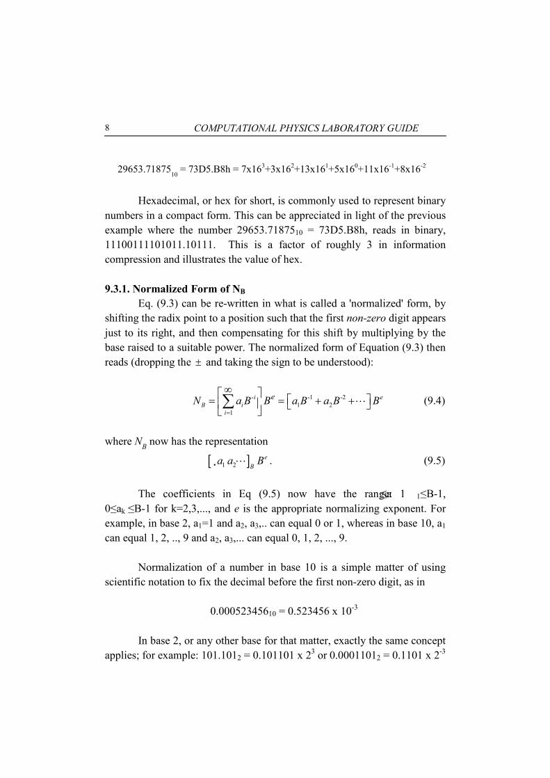
29653.7187510 = 73D5.B8h = 7x163+3x162+13x161+5x160+11x16-1+8x16-2

Hexadecimal, or hex for short, is commonly used to represent binary

numbers in a compact form. This can be appreciated in light of the previous example where the number 29653.7187510 = 73D5.B8h, reads in binary, 11100111101011.10111. This is a factor of roughly 3 in information compression and illustrates the value of hex. 9.3.1. Normalized Form of NB

Eq. (9.3) can be re-written in what is called a 'normalized' form, by shifting the radix point to a position such that the first non-zero digit appears just to its right, and then compensating for this shift by multiplying by the base raised to a suitable power. The normalized form of Equation (9.3) then reads (dropping the ± and taking the sign to be understood):

- -1 -21 2

1

i eB i

i

eN a B B a B a B B=

∞ = = + + ⋅⋅⋅ ∑ (9.4)

where NB now has the representation

[ ]• 1 2e

Ba a B⋅ ⋅ ⋅ . (9.5)

The coefficients in Eq (9.5) now have the range: 1≤a 1≤B-1,

0≤ak ≤B-1 for k=2,3,..., and e is the appropriate normalizing exponent. For example, in base 2, a1=1 and a2, a3,.. can equal 0 or 1, whereas in base 10, a1 can equal 1, 2, .., 9 and a2, a3,... can equal 0, 1, 2, ..., 9.

Normalization of a number in base 10 is a simple matter of using

scientific notation to fix the decimal before the first non-zero digit, as in

0.00052345610 = 0.523456 x 10-3

In base 2, or any other base for that matter, exactly the same concept applies; for example: 101.1012 = 0.101101 x 23 or 0.00011012 = 0.1101 x 2-3


The importance of normalization lies in the fact that computers represent numbers containing decimals, that is, 'floating-point' numbers, using some method of normalization. We will return to this topic later when we discuss the storage of these numbers in computer memory.

It should also be clear that the largest value that NB can represent, for a given exponent, corresponds to the situation where all of the coefficients in Equation (9.5) are set equal to B-1, while the smallest non-zero number occurs when a1=1 and all of the other coefficients equal zero.

9.3.2. Precision [Ko93]

As indicated, Eq (9.3) can, in principle, represent any number without approximation. However, there are times where we have no choice but to limit, or approximate the number of digits in a number. For example, this will happen whenever a number is irrational like π , e or 2 , or when the number contains an infinite number of repeating digits such as 1/3 or 2/3, or, from an experimental point of view, when the accuracy of the number is the limiting factor.

We denote this limiting of the length of the number NB to a precision of p digits, by re-writing Eq (9.4) to read,

1 21 2

1

i e p eB i p

i

p

N a B B a B a B a B B− − −

=

≅ = + + ⋅⋅⋅+

∑ (9.6)

Clearly, for a fixed value of p, if a number has p or fewer digits, it

can be represented exactly; otherwise its representation will be approximate. For example, π, correct to a precision of 6 base 10 digits, would be written according to Eq (9.6) as:

π

=

≅ = =

1

1

2

0.314159 x 10 (base 10,p 6)

0.1100100100001111111 x 2 (base 2,p 19)

0.3243F9 x 16 (base 16,p 6)


whereas π is approximated as 3.125 if expressed to a precision of 6 binary digits. Comment

Certain binary numbers like 6.610 = 110.100110012…, or 0.110 = 0.0001100110011002…, are the binary equivalents of a non-terminating base 10 fraction like 1/3. These numbers have no exact binary image which means that it will be impossible to exactly represent them in a computer no matter how many bits are available for storage. It is also interesting to note that the non-terminating feature of a fraction is a function of the base in which the number is represented. Table 9.2 illustrates this point with the base ten fraction 2/3.

Table (9.2) 2/3 to Different Bases

BASE REPRESENTATION 2 0.1010101... 3 0.2 4 0.2222222... 5 0.3131313... 6 0.4 7 0.4444444... 8 0.5050505.. 9 0.6 10 0.6666666...

The reader might find it instructive to extend Table 9.2 through base 16.

9.3.3. Computer Memory and Binary Number Storage [Ko93] We have just seen that the larger the base, the greater the amount of information carried by each digit. Thus, as we have just seen, π to six digits in base 10 requires 19 digits in binary; and a trillion (1x1012) requires 13 base 10 digits and some 39 base 2 digits. In general it takes roughly 3 binary digits to represent a single base 10 digit. However, inefficiency aside, it is precisely because binary has only two possible coefficients, 0 and 1, that it is ideal for representation by a two-state device. These two states might, for


example, be represented by the conducting or non-conducting modes of a solid state device like a diode.

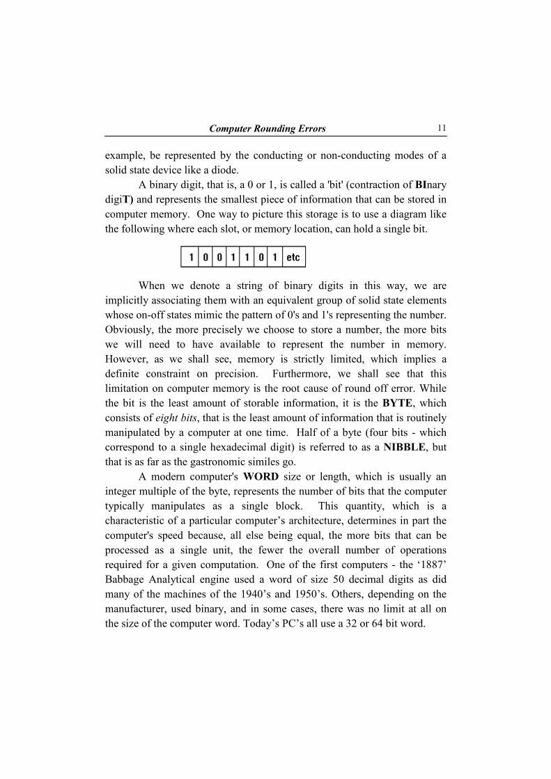
A binary digit, that is, a 0 or 1, is called a 'bit' (contraction of BInary digiT) and represents the smallest piece of information that can be stored in computer memory. One way to picture this storage is to use a diagram like the following where each slot, or memory location, can hold a single bit.

When we denote a string of binary digits in this way, we are

implicitly associating them with an equivalent group of solid state elements whose on-off states mimic the pattern of 0's and 1's representing the number. Obviously, the more precisely we choose to store a number, the more bits we will need to have available to represent the number in memory. However, as we shall see, memory is strictly limited, which implies a definite constraint on precision. Furthermore, we shall see that this limitation on computer memory is the root cause of round off error. While the bit is the least amount of storable information, it is the BYTE, which consists of eight bits, that is the least amount of information that is routinely manipulated by a computer at one time. Half of a byte (four bits - which correspond to a single hexadecimal digit) is referred to as a NIBBLE, but that is as far as the gastronomic similes go.

A modern computer's WORD size or length, which is usually an integer multiple of the byte, represents the number of bits that the computer typically manipulates as a single block. This quantity, which is a characteristic of a particular computer’s architecture, determines in part the computer's speed because, all else being equal, the more bits that can be processed as a single unit, the fewer the overall number of operations required for a given computation. One of the first computers - the ‘1887’ Babbage Analytical engine used a word of size 50 decimal digits as did many of the machines of the 1940’s and 1950’s. Others, depending on the manufacturer, used binary, and in some cases, there was no limit at all on the size of the computer word. Today’s PC’s all use a 32 or 64 bit word.


9.4. HISTORICAL INTERLUDE: CPUs, COPROCESSORS AND ALL THAT [Hmc], [Ov01]

Before continuing with our development of the subject of computer error, it is worth pausing to make a few comments on how computers do arithmetic at the machine level. The following description will be confined to the operation of the PC, partly because of its ubiquity but also because the PC shares basic features common to all computers so there is no significant loss of generality when describing its operation.

The heart of any computer is its central processing unit or CPU for short. In the case of the IBM PC, the CPU chips that form the heart of the series (designated as the 80x86 family) consist of three parts: an arithmetic and logic unit, or ALU, timing and control circuits and a series of registers.

For example, the INTEL 8088 CPU, which was the microprocessor used in the original PC, had some fourteen 16 bit registers. Of these fourteen, the four scratch-pad registers are used as a temporary working area, particularly for arithmetic operations. The other 10 registers perform a variety of duties, such as keeping track of where current data and program code are located in memory.

The instruction set for the 8088 chip supported only single and double precision integer addition, subtraction, multiplication and division. This means that if we want to do arithmetic with real, or floating-point numbers, which are numbers containing decimals, we must do so by writing software routines that tell the CPU, in precise detail, exactly how to do this arithmetic. The solution to this vexing problem was the introduction of the Intel 8087 math coprocessor chip which was designed to handle floating point arithmetic operations without the need for additional software, and which was designed to function in combination with the 8088 chip.

However, before we can worry about the issue of how to do arithmetic with floating-point numbers, we must first decide on how to represent these numbers in memory. This is not a trivial problem as evidenced by the many different and incompatible formats used by computer manufactures over the years and well into the 1970’s. The obvious need for a consistent format resulted in extensive collaborations from the late 1970’s to the early 1980’s between academic computer scientists and their counterparts in the computer industry. The outcome of this remarkable


cooperation was the eventual adoption of the ANSI/IEEE (ANSI = American National Standards Institute, IEEE = Institute for Electrical and Electronics Engineers) Standard published in 1987 and known as the ANSI/IEEE Std 854-1987. The Standard specifies, in great detail, the accuracy with which computations are to be done, how rounding is to be carried out, error and exception handling and how numbers are to be represented in memory as well as other issues germane to accurate floating-point arithmetic. Incidentally, the ANSI/IEEE standard does not address how integers are stored in computer memory.

As mentioned earlier, in 1980, and well prior to the final 1987 ANSI/IEEE Standard, the Intel Corporation produced the first math coprocessor, the 8087. The 8087 implemented the ANSI/IEEE Draft Standard in a single integrated circuit that worked in conjunction with the 8088 CPU. The primary purpose of the coprocessor was to enable the computer to do highly accurate and very fast floating-point arithmetic. As a result, the IBM PC was transformed from a machine that was largely undistinguished from the competition to a computer that was able to perform computations that had previously belonged to the world of mainframes. Since the 8087, a math coprocessor has since been produced for each new member of the 80x86 family (through the 80386), of CPU's, and in each case, the chip implemented the ANSI/IEEE Standard for Binary Floating-point Arithmetic.

Starting with the 80486 DX, the math coprocessor became an integral part of the CPU and given the name ‘floating point unit’, or FPU for short. This integration made floating point computations much faster and more efficient. Each coprocessor or FPU, and its corresponding CPU, shares the same address and data bus permitting the coprocessor to constantly monitor the CPU's data stream. When a special 'escape code' is encountered, the coprocessor knows that a floating-point instruction is on the way, and can act accordingly.

Like the CPU, the coprocessor also has a number of registers that provide the workspace for computation, as well as an elaborate instruction set that can be manipulated through assembly language routines. This instruction set includes the basic addition, subtraction, multiplication, division and square root operations, as well as a number of auxiliary


operations like rounding, absolute value etc. There are also a number of specialized instructions, which are very coprocessor model dependent. These include instructions for operating with logarithmic, exponential, trigonometric and hyperbolic functions.

The exact number and function of the coprocessor registers is a function of the specific chip, but they all contain at least eight numeric data registers (the IA 64 bit Itanium chip has, for example, 128 registers), each of which is 80-bits wide. These are used to hold numeric operands in what is called 'extended precision'. The relevance of this statement, and we shall come back to this later, is that the coprocessor does extended precision arithmetic using 80-bits to represent each floating-point number. The numeric result of a computation is then stored in 32 or 64-bit memory. Since arithmetic is done with much greater precision than the subsequent storage of the result, we can make the assumption that basic floating-point arithmetic operations are exact. The importance of this assumption will be clear later when we discuss extended floating-point arithmetic.

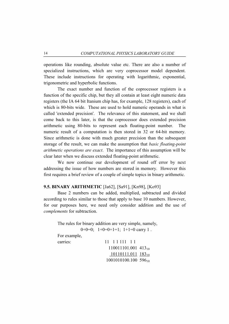
We now continue our development of round off error by next addressing the issue of how numbers are stored in memory. However this first requires a brief review of a couple of simple topics in binary arithmetic. 9.5. BINARY ARITHMETIC [Ja62], [Sa91], [Kn98], [Ko93]

Base 2 numbers can be added, multiplied, subtracted and divided according to rules similar to those that apply to base 10 numbers. However, for our purposes here, we need only consider addition and the use of complements for subtraction.

The rules for binary addition are very simple, namely,

0+0=0; 1+0=0+1=1; 1+1=0 carry 1 . For example, carries: 11 1 1 111 1 1

110011101.001 41310 10110111.011 18310 1001010100.100 59610


9.5.1. Complements/Subtraction Most computers store negative numbers in what is called two's complement form. The motivation for this method of representation is that it allows the computer to treat addition and subtraction identically in that borrowing between columns is unnecessary. This has advantages from the viewpoint of hardware design.

The definition of two's complement is based on the requirement that in order for the sum of two numbers to be zero, one number must be the negative of the other. That is, any positive number plus its complement is zero, provided that the number of bits used to represent the number and its complement is fixed by the size of the computer's storage registers so that any overflow bit will be automatically discarded.

9.5.2. Rules for Constructing Two's Complement

Given a binary number N2, the two's complement is formed by the procedure:

1. Begin by right justifying your number to match the word size. If the number is less than the word size, add zeros to the left to fill the allotted space. Now change all of the 1's to 0's, and all of the 0's to 1's. This is called “one's complement”.

2. Add 1 to the least significant bit (i.e., the right-most bit). We now have “two's complement”. This result when added to another base 2 number is equivalent to subtraction provided the top bit is discarded if it exceeds the word size. From a hardware point of view, it is much easier to subtract by adding complements than use the ‘carry’ method common to base 10 subtraction.

By way of example, consider the simple case of 16-5=11, i.e., 10000-00101 in base 2. Assuming a 5 bit storage register, we obtain the complement of 00101 using our rules to get 11011 which, when added to 10000 gives 01011 = 11. It is easy to see the advantage of complements from a hardware point of view.


9.6. INTERNAL STORAGE OF NUMBERS Computers distinguish between how they store integers and floating-

point numbers. 9.6.1. Integers

The number of bits used for integer storage is usually the same as the computer's word size. For example, a computer with a 32 bit word will use 32 bits for the storage of every integer whose length does not exceed 32 bits, and, in addition, that storage is exact. 9.6.2. Properties of Stored Integers

One may easily verify that the range and number of integers, I, compatible with a computer of word length w, using two's complement storage for negative integers and a signed first bit, is:

• range of integers: -2

w-1 ≤ I ≤ 2w-1

-1 • total number of positive or negative integers: 2

w-1

• total number of positive and negative integers: 2w

For example, suppose we have a computer with 4 bit word,

(i.e., w=4) of which the first bit is the sign bit leaving 3 bits available for integer storage.

Thus, our integers can range from -23 to 23-1, or -8≤ I≤7. The other two properties tell us that there are 8 of each sign (0 is taken as positive) for a total of 24= 16. Using two's complement for the negative integers, we have:

1000, 1001, 1010, 1011, 1100, 1101, 1110, 1111, 0000, 0001,…, 0111

-8 -7 -6 -5 -4 -3 -2 -1 0 +1 +7

Note that each negative number is constructed from its positive equivalent by taking the two's complement, and that each number and its complement add to zero. The negative sign is taken care of automatically since we have chosen to represent a positive integer by a 0.


9.6.3. Integer Storage Details [K093], [Sa91] There are different ways to store integers, but it is most common to

store positive integers directly as written in binary and then use two's complement for the negative integers. The numbers are then stored 'right justified' in word length registers with zeros added to the left to fill the unused storage locations. The first bit is used to represent the sign of the integer, and is either a 0 (said to be 'unset') if the number is positive, or a 1 ('set'), if negative as we have already indicated.

For example, the number 437 base 10 would be stored in a 16 bit

register as:

whereas - 437 would be represented using two's complement, as:

Note that in constructing the two's complement from the positive

integer, the filler 0's are also changed to 1's, and that the sign bit is now a 1. An alternative, but less common format to the use of two's

complement is to store a negative integer in exactly the same form as a positive integer except for a 'set' leading bit to indicate a negative number. Representation of positive and negative numbers in this fashion is termed 'sign-magnitude' format.

9.6.4. Floating-Point Numbers [Ov01], [Go91]

Floating-point numbers or ‘real’ numbers are ones that contain decimals. As we indicated, the primary purpose of the ANSI/IEEE Std 854-1987, apart from addressing the need for consistency, was to make floating-point arithmetic and storage as accurate and predictable as possible.


a) Definition of a Floating-point Number A base 2 floating-point number, N2, is expressed as the product

N2 = f * 2e and consists of two parts - a signed normalized fractional part, f, and a signed integer exponent, e. Here the normalized fraction f is called the significand or mantissa, and has a range of values that depends on the method of normalization. b) Normalization

We have already introduced the concept of normalization with the comment that floating-point numbers are stored this way. The question is why?

First - there has to be a binary point somewhere and that 'somewhere' must be pre-determined in a consistent fashion for all possible floating-point numbers. This is because there is no way to specifically designate the binary point in memory apart from using ones and zeros which are already used to represent the number itself. The obvious solution is then to fix the absolute position of the binary point in the storage register and then force the number to conform to this format.

Second - fixing the binary point at the beginning of the number maximizes its precision by maximizing the number of bits used for its representation. We are now ready to see how floating-point numbers are stored.

There are two common methods of normalization. The procedure introduced earlier, and which we will call, for lack of better phrase, the Non-Standard format, fixes the binary point just before the first non-zero digit, and the ANSI/IEEE Standard, which recommends fixing the binary point just after the first non-zero digit. For example, the binary number, 101.101 would be normalized as 0.101101 x 23 according to the Non-Standard format, and as 1.01101 x 22 using the Standard format. The Standard also calls for suppressing the leading bit (since it is always a 1) so the number is now be written .01101 x 22. Since storage registers are of fixed length, this


has the advantage of increasing the available storage, and hence the precision, by one additional bit.

Table 9.3 summarizes the properties of these two methods of normalization. Table (9.3) Common Normalization Methods

FORMAT RANGE OF f2 RANGE OF f10 FORM OF N2

NON-STANDARD 0.100..02 to 0.111..12 (1/2 ≤ f10 < 1) N2 =.1ddd..d * 2e

ANSI/IEEE 1.000..02 to 1.111..12 (1 ≤ f10 < 2) N2 =.dddd..d * 2e

The reason we introduce the alternative to the ANSI/IEEE

normalization format is that it is common to most texts that discuss floating-point arithmetic and round off error. It is also less awkward from the viewpoint of notation than the ANSI/IEEE Standard with its repressed leading bit and de-normalized numbers to accommodate gradual underflow etc. Since the method of normalization is unimportant as it pertains to the origin of round off error, we will often use Non-Standard normalization for purposes of illustration. Care will be taken to specify which method is being used.

Depending then on the method of normalization, our binary number

N2, will be written, ≤

= ≤ <

10

102

e 1/2 f <1 Non-StandardN f 2 where *

1 f 2 ANSI/IEEE (9.7)

c) Floating-point Storage

With Non-Standard Normalization and Eq (9.6), we can write an arbitrary binary number to a precision of p digits as:

i e 1 2 p e2 i 1 2 p 1 k

p

i 1N a 2 2 a 2 a 2 a 2 2 where a 1, a 0 or 1 for k > 1− − − −

=

= = + + ⋅⋅⋅+ = =

∑ ,

which on comparison with Eq (9.7) identifies the normalized fraction f, as the sum:


i 1 2 pi 1 2 p

p

i 1f a 2 a 2 a 2 a 2− − − −

== = + + ⋅⋅⋅+∑ (9.8)

Since, according to Eq (9.5), the binary representation of N2 is just the set of coefficients in Eq (9.8), each of which is stored as a single bit, it follows that the precision p, in Eq (9.8) can be identified as the number of bits used to store N2. Clearly then, the more bits available for storage, the greater the precision.

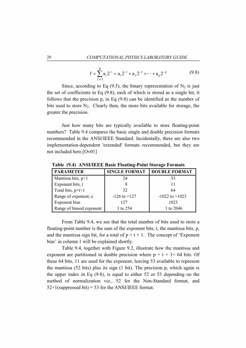
Just how many bits are typically available to store floating-point numbers? Table 9.4 compares the basic single and double precision formats recommended in the ANSI/IEEE Standard. Incidentally, there are also two implementation-dependent 'extended' formats recommended, but they are not included here.[Ov01] Table (9.4) ANSI/IEEE Basic Floating-Point Storage Formats

PARAMETER SINGLE FORMAT DOUBLE FORMAT Mantissa bits, p+1 24 53 Exponent bits, t Total bits, p+t+1

8 32

11 64

Range of exponent, e Exponent bias

-126 to +127 127

-1022 to +1023 1023

Range of biased exponent 1 to 254 1 to 2046 From Table 9.4, we see that the total number of bits used to store a

floating-point number is the sum of the exponent bits, t, the mantissa bits, p, and the mantissa sign bit, for a total of p + t + 1. The concept of ‘Exponent bias’ in column 1 will be explained shortly.

Table 9.4, together with Figure 9.2, illustrate how the mantissa and exponent are partitioned in double precision where p + t + 1= 64 bits. Of these 64 bits, 11 are used for the exponent, leaving 53 available to represent the mantissa (52 bits) plus its sign (1 bit). The precision p, which again is the upper index in Eq (9.8), is equal to either 52 or 53 depending on the method of normalization viz., 52 for the Non-Standard format, and 52+1(suppressed bit) = 53 for the ANSI/IEEE format.


Figure (9.2) Double Precision Storage Format

From Figure 9.2, we see that bit m1 is reserved for the sign of the

mantissa, bits e1 through e11 are used to store the exponent e, usually in biased form, and bits m2 to m53 represent the mantissa in normalized form. As drawn, Figure 9.2 represents the Non-Standard format. The ANSI/IEEE Standard would modify Figure 9.2 by repressing bit m2 , which is a 1, and then shifting each of the bits from m3 to m53 left one slot. This leaves m53 available for storage of an additional bit that would not be available in the Non-Standard format. The exponent is also modified since e is now one less than in the Non-Standard format. We now look at this storage process in greater detail. d) Coding the exponent

The exponent e is an integer, which may be positive or negative, and may be stored using the formats we have already discussed for integers. However, there are disadvantages with these schemes. Whenever two numbers are to be added or subtracted, a comparator must be used to determine the magnitudes of the exponents. This is because, just as is the case in scientific notation, the exponents must agree before addition or subtraction can be carried out. This comparison process would be less complicated if the exponents were always positive. e) Exponent Bias

The exponent bias (also called the “excess”) is defined in such a way as to ensure that the biased exponent is always positive, namely,

biased exponent ≡ b.e. = e + bias

The following examples illustrate how biasing works.


(i) Since e is an integer, it can be represented by the exponent range characteristic of integer storage using two's complement,

-2

t-1≤ e≤ (2

t-1) -1 (9.9)

where t is the number of bits used to store the exponent. Since the least exponent is -2

t-1, we define the bias as +2

t-1, so our biased exponent now

reads:

b.e. = e + 2t-1

which is always positive. For example, according to Table 9.4, if we take t = 11 (double precision), then our bias is 210 = 1024, the biased exponent is given by,

b.e. = e + 1024

and we would describe the storage of the exponent in terms of “excess 1024” notation. Furthermore, the biased exponent now has the range 0≤b.e.≤2047 corresponding to -1024≤ e≤1023. Note that negative values of e correspond to values of b.e. < 1024.

(ii) Alternatively, if we take the ANSI/IEEE double precision bias*

of 1023 from Table 9.4, our biased exponent would read

biased exponent = e + 1023 In this case, 1≤b.e.≤2046 corresponding to the exponent range

given in Table 9.4. Here, values of the biased exponent less than 1023 correspond to negative values of e. The bias might seem complicated, but all we are doing is ensuring that the least exponent is positive.

* The ANSI/IEEE Standard bias and exponent range differ from that given by Eq 9.9 in order to ensure that the reciprocal of any normalized floating-point number does not cause underflow.


f) Storing the Exponent In any case, once the exponent has been biased it is then converted to

binary, and stored right-justified using bits e1 through e11 (or e1 through e8 in single precision) in the exponent field. A sign bit is now unnecessary since biased exponents are always positive. g) Storing the Mantissa

The mantissa is usually stored left justified by encoding the number in sign-magnitude format, i.e., exactly as written in binary with a signed first bit. The sign of the mantissa is fixed by the value of the bit m1, which is 0 if positive and 1 if negative. This whole process is considerably more difficult to describe than it is to perform as the following example illustrates. EXAMPLE (9.5)

Suppose we want to code the number -50.375 in single precision (t=8), using both the ANSI/IEEE Standard, and the Non-Standard format, for comparison. The Non-Standard bias will be based on Eq (9.9) and the ANSI/IEEE bias is taken from Table 9.4 using the following procedure: a.Write the number in normalized binary form: -50.37510 = - 110010.0112 = - .1100100112 x 26 NON-STANDARD = - 1.100100112 x 25 ANSI/IEEE b. Bias the exponent: b.e. = e + 2

t-1 = 6 + 28-1 = 13410 = 100001102 NON-STANDARD - Eq 9.9

b.e. = e + 127 = 5+127 = 13210 = 100001002 ANSI/IEEE - Table 9.4 c. Write the mantissa as it will be coded: f = 1 110010011 NON-STANDARD f = 1 100100110 ANSI/IEEE

The underlined 1 denotes that our number is negative. Note that the leading bit for the ANSI/IEEE format has been dropped so an extra 0 must be added to the end of the number. We now store our number using left-justification for the mantissa:


NON-STANDARD

ANSI/IEEE

These storage formats can also be represented using hexadecimal notation: C3h 64h C0h 00h Non-Standard C2h 49h 80h 00h ANSI/IEEE where each group of two hex digits represents one byte. We now turn our attention to the properties of these stored numbers, and how those properties make round off error a virtual certainty in almost all computations. 9.6.5. Properties of Floating-Point Numbers [FMM], [M&H78]

Everyone is familiar with the fact that 'real numbers' form an infinite continuum, that is, they are both continuous, and infinite in extent. Unlike the real number system, however, the range of numbers that a computer can store (that is, computer numbers as distinct from real numbers) is neither infinite nor continuous. In fact, the totality of floating-point numbers available to a computer is a function of its design, and can be computed exactly from the following relationship:

( ) −= − − + +max min max min

p 1F(B,p,E ,E ) [2 B 1 B (E E 1)] 1 . (9.10)

B is the number base, p the number of bits available for storage of the mantissa, exclusive of sign, and Emax and Emin are the largest and smallest values of the exponent e, that is, Emin ≤ e ≤Emax .

Justification of Equation (9.10)

Assuming Non-Standard normalization, then, if we have p bits available to store the normalized mantissa, it follows that the first digit can


be any one of B-1 possibilities (e.g., 1 in binary or 1,2,..,9 in radix 10). This leaves p – 1 bits, each of which can take on B values (e.g., 0,1 in binary or 0,1,2,..,9 in radix 10). However the number of permutations of B numbers taken p-1 at a time is exactly Bp-1 so the total number of possible combinations of mantissa digits is 2(B-1)Bp-1, where the 2 accounts for both positive and negative values. Note that as yet, 0 has not been included since the leading digit is non-zero as required by Non-Standard normalization.

Now the number of integer values the exponent e can have is just the “exponent range +1”, that is: Emax-Emin +1. Since each of the mantissa values, is multiplied by each value of the exponent, we finally have Eq (9.10), after adding 1 to account for 0.

Taking B=2, and assuming Eq. (9.9) represents the exponent range, Eq (9.10) reduces to the simple expression:

− − + − − = + 1 1t t p tF 2,p,2 1, 2 2 1 . (9.11)

Since the number of bits available to store a floating-point number is

just p+t+1, we conclude that the range of floating-point numbers is dependent only on this sum, and not on how the available bits are partitioned between the exponent and the mantissa.

To illustrate the distinction between real numbers and computer

numbers, we will calculate the set of computer numbers available in a hypothetical computer whose storage format consists of a three bit mantissa, (p = 3), and a 2 bit exponent (t = 2). For simplicity, the sign will be designated as ± instead of a binary digit. From Eq (9.11), we find that our computer can represent exactly 33 real numbers, that is, there are exactly 33 computer numbers available in this computer to represent the entire infinite range of real numbers. Table 9.5 lists this set.


Table (9.5) Computer Numbers in the Set F(2, 3, 1, -2)

Table 9.5 also exhibits a number of interesting and important

features of the floating-point number system. a) Density of Numbers

We observe that the difference between numbers of like exponent is constant, i.e., 0.03125 for 2-2, 0.0625 for 2-1, 0.125 for 20 and 0.25 for 21, and in addition, each factor of 2 increase in the exponent also doubles the separation between these numbers. Thus, as we move away from the origin, floating-point numbers become increasingly sparse. This is in direct contrast with the behavior of the integers which map with uniform spacing. This increase in sparseness implies that the larger the real number to be stored, the lower the probability of an exact match with an existing

MANTISSA EXPONENT COMPUTER NUMBER .000 0 02 = 010 ± .100 -2 ±.001002 = ±0.12500 ± .101 -2 ±.001012 = ±0.15625 ± .110 -2 ±.001102 = ±0.18750 ± .111 -2 ±.001112 = ±0.21875 ± .100 -1 ±.01002 = ±0.2500 ± .101 -1 ±.01012 = ±0.3125 ± .110 -1 ±.01102 = ±0.3750 ± .111 -1 ±.01112 = ±0.4375 ± .100 0 ±.1002 = ±0.5000 ± .101 0 ±.1012 = ±0.6250 ± .110 0 ±.1102 = ±0.7500 ± .111 0 ±.1112 = ±0.8750 ± .100 1 ±1.002 = ±1.000 ± .101 1 ±1.012 = ±1.250 ± .110 1 ±1.102 = ±1.500 ± .111 1 ±1.112

= ±1.750


computer number. Figure 9.3 illustrates this behavior for a portion of F(2, 3, 1, -2). The line to the left of ‘0’ is identical to the positive line, only negative.

- . 2 5 - . 1 2 5 0 . 5 1. 1 2 5 . 2 5 1 . 7 5

Figure ( 9.3) Plot of a Portion of the Set F(2,3,1,-2)

We see that our hypothetical computer is very limited indeed. Even

in a computer with 32 or more bits dedicated to floating-point storage, the set of possible computer numbers is minuscule relative to the set of real numbers. For example, assuming 64 bit storage, we calculate from Eq (9.11) that a computer has approximately 10

19 computer numbers

available. Clearly an improvement, but hardly the infinite set needed to represent the real numbers.

The next question is, what happens when we try to store a real number that does not coincide with one of the allowable set of 33 belonging to F(2, 3, 1, -2)? This question has several answers, which, taken collectively, constitute the cause of rounding error. b) Underflow

From Fig 9.3, we note that there exists a considerable gap between 0 and the first computer number 2-3. Any real number that falls in this underflow gap will be automatically set equal to 0.*

* An alternative procedure supported by the ANSI/IEEE Standard, and called “gradual underflow”, consists of uniformly filling the underflow gap with numbers whose absolute spacing is identical to that between Xmin and 2*Xmin. Table 9.6 compares the least non-zero number for a PC, with and without a math co-processor, using double precision storage.

Usually this

Table (9.6) Least Non-Zero Number in Different Implementations No Coprocessor – compiler dependent result 5.56 x10-309 Coprocessor present, gradual underflow not implemented by compiler 2.22 x10-308 Coprocessor present, gradual underflow is implemented 4.94 x10-324


approximation does not terminate execution, or even evoke a warning, although the process can be potentially serious because of the automatic elimination of all significant digits.

It should be noted that this underflow gap exists because of our use of a normalized mantissa (irrespective of the method of normalization) which automatically defines a first non-zero number, Xmin (0.125 in our example). The origin of this gap will make more sense if we calculate its value theoretically. To keep the notation simple, we will, without loss of generality, base the argument on Non-Standard normalization.

c) Calculation of the First Non-Zero Number

From Eq. (9.7), it follows that the first positive number greater than zero is:

Xmin = fmin 2

Emin

where fmin is the smallest non-zero mantissa and Emin is the smallest possible value of the exponent e. According to Non-Standard normalization, fmin must be fmin = (.1000··)2 = (2-1)10 Since Eq (9.11) was derived using the exponent range given by Eq (9.9), we must take Emin = -2

t-1 , in which case:

( )−−=

t 1-1

min

2X 2 2 (9.12)

Since t = 2 for our hypothetical computer, we have:

Xmin = 2-1×2-2 = 0.125 in agreement with our result in Table 9.5. d) Overflow

At the other end of the scale, real numbers that exceed our largest computer number of 1.75 will not be stored. However, unlike underflow, an


error will probably be raised resulting in program termination accompanied by an overflow warning.

Like the least number, the computer's largest number can also be computed theoretically and it is instructive to do so. e) Calculation of a Computer’s Largest Number

In this case Xmax = fmax 2 Emax

Now fmax is maximum when all p mantissa bits are set to 1, so

−

== =∑ i

max 2

p

i 1f 2 (.1111....)

But ip

i 1 2−

=∑ is just a geometric progression whose sum is 1-2-p, so:

fmax = 1-2-p

Again using Eq. (9.9), we have: Emax = (2t-1)-1, or:

−− −= − t 1p (2 1)

maxx (1 2 )2 (9.13)

Finally, for our hypothetical computer, where p=3 and t=2, we calculate that xmax = 1.7510 , which again confirms our previous calculations.

Eqs (9.12) and (9.13) give the smallest and largest positive computer

numbers belonging to the set F(2, 3, 1, -2). These same conclusions apply to negative values of F(2, 3, 1, -2). 9.7. ROUNDING, CHOPPING, AND THEIR ERROR BOUNDS [Ov01], [Go91], [Ja62]

As sources of computer error, underflow and overflow are relatively unimportant since the frequency of their occurrence is usually rare. Of far greater importance is the question of how real numbers that do not cause underflow or overflow are represented, that is, real numbers that fall within


the computer’s minimum and maximum range, but do not exactly match any of the allowable set of computer numbers. [Ja62], [Go91]

The solution is for the computer to force a fit by either rounding or

chopping the real number to match the closest computer number. This mapping of the real number to its closest computer equivalent is the origin of what is usually meant by the term “round off error”, and is a natural consequence of limited computer memory. Indeed, it is the point of this chapter. We define rounding and chopping as follows: 9.7.1. Chopping

Chopping is an accurate description of exactly what one does to reduce a number to one with fewer digits - you simply delete or chop all unwanted digits. Put another way, chopping is just rounding towards zero, which means that a chopped positive number decreases in magnitude, and a chopped negative number, increases.

In our hypothetical computer, where p = 3 - see Table (9.5) - the real number 0.3749 would be mapped to 0.3125 with an error of 17%, i.e., chop 0.374910 = .10112··· x 2-1 .101 x 2-1 0.312510 9.7.2. Rounding

Rounding a number to p mantissa bits involves the procedure in which the computer retains p+1 bits, adds 1 to the (p+1)th bit*

and then chops to p bits. This is equivalent to the familiar process in base 10 of adding 5 to the number following the rounding digit, and then chopping. Rounding is done after normalization in order to preserve accuracy.

Rounding in our hypothetical computer would map 0.3749 to 0.3750 with an error of less than 1%, i.e. +.0001:

chop .374910 = .10112 x 2-1 .1100 x 2-1 .110 x 2-1 0.375010

* More generally, for an arbitrary base B, add B/2 B-(p+1) Be


Rounding, while considerably more accurate than chopping, has a significantly greater computational overhead. For that reason, and because for many applications the distinction is relatively unimportant, chopping is not uncommon. However, any computer that supports the ANSI/IEEE standard will use rounding.

We conclude this section by reiterating that round off error will occur whenever a real number does not belong to the set F(B, p, Emax, Emin), and must therefore be rounded or chopped to agree with its closest computer approximation. It is also important to realize that even if two real numbers happen to map exactly it is unlikely that there sum, product etc. will. For example, the sum of the two numbers, .101 x 21 and .100 x 2-2, both of which belong to our set of 33 listed in Table 9.5, is .1011 x 21 (=1.37510) and which is not a member of the set.

Since round off error is a virtual certainty for almost any digital computation, the issue is not how to avoid it, but rather, how to live with it. Our first step, to that end, is to establish a quantitative measure of its impact.

9.7.3. Error Bounds

We have already seen that a base 2 floating-point number x can be written in the normal form:

FL(x) = f*2e (9.14)

where we use FL(x) to represent the computer number equivalent of the real number x. Thus FL(x) belongs to the set F(B, p, Emax, Emin) while x may or may not. In a loose sense, we will view FL as a kind of operator whose function it is to map a real number x into the set F(B, p, Emax, Emin) through the aegis of chopping or rounding.

In order to estimate the error associated with this mapping process, we first calculate the separation between two arbitrary nearest-neighbor computer numbers. Then, assuming that the real number x falls between these two computer numbers, we calculate the error incurred when we chop or round x to force agreement with one of them.

Taking the mantissa to be exactly .100…, assuming normalization, we can, without loss of generality, define the smallest floating-point numbers greater than 0 to be


FL(xi) = 2-1 × 2e

Then, assuming p mantissa bits, the value of the next largest mantissa must be a set pth bit or 2-p. This number, when multiplied by 2e and added to FL(xi), will generate the next larger computer number FL(xi+1),

FL(xi+1) = (2

-1 + 2-p) 2e .

The gap between these two successive computer numbers is then the difference:

δ = FL(xi+1) - FL(xi) = 2e-p (9.15)

Consider now a positive real number x that falls between FL(xi) and FL(xi+1), i.e.:

FL(xi)≤ x ≤FL(xi+1) The following diagram illustrates how these numbers are related. Figure (9.4) Relationship between x and FL(x)

If we assume that x will be approximated by the closest computer

number, then rounding will set x equal to FL(xi+1) for x to the right of the midpoint, and FL(xi) if chopping is used. Figure 9.4 also establishes the following relationship between the absolute error bound and the gap size,

δ

δ= − ≤

choppingAE x FL(x)

2 rounding . (9.16)

Thus the difference between x and its floating-point equivalent, FL(x) will be bounded by the full gap if chopping is used, and by half of the gap size for rounding. Since one might expect that on average, real numbers


falling within the gapδ would be evenly distributed, one will appreciate just how pessimistic the chopping bound can be.

We next establish the relationship between the gap size, the machine precision p, and x itself. To do this we specify how the mapping is achieved. 9.7.4. Rounding Error Bound

From Eq (9.15), it follows that

δ /2 = 1/2 * 2e-p = 2-p * 2e-1

or, using Eq (9.16) and the fact that FL(xi) = 2e-1 gives

|x-FL(x) | ≤ 2-p * 2e-1 .

In addition, since x is assumed to fall between FL(xi ) and FL(xi+1), then the least bound for arbitrary x is, from Fig 9.4,

FL(xi)≤ |x|

from which we can we conclude that the absolute error bound for x is:

AE = |x-FL(x)| £ |x| 2-p

(9.17)

Equation (9.17) says that the absolute error with which x is stored is a function of the magnitude of the x itself and the machine precision.

In contrast, the relative error, which follows from Eq (9.2), is:

≤ -px-FL(x)RE= 2

x

and which is seen to depend on the machine precision but not on x itself. 9.7.5. Chopping Error Bounds Since, according to Eq. (9.16), the error associated with chopping and rounding differ by a factor of 2, it follows that the absolute chopping error is given by:


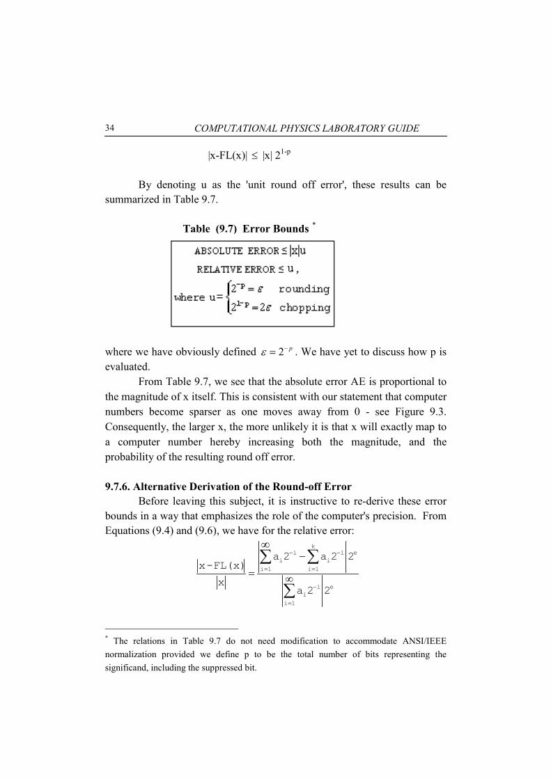
|x-FL(x)| ≤ |x| 21-p

By denoting u as the 'unit round off error', these results can be summarized in Table 9.7.

Table (9.7) Error Bounds *

where we have obviously defined 2 pε −= . We have yet to discuss how p is evaluated.

From Table 9.7, we see that the absolute error AE is proportional to the magnitude of x itself. This is consistent with our statement that computer numbers become sparser as one moves away from 0 - see Figure 9.3. Consequently, the larger x, the more unlikely it is that x will exactly map to a computer number hereby increasing both the magnitude, and the probability of the resulting round off error.

9.7.6. Alternative Derivation of the Round-off Error

Before leaving this subject, it is instructive to re-derive these error bounds in a way that emphasizes the role of the computer's precision. From Equations (9.4) and (9.6), we have for the relative error:

− −

= =

−

=

∞

−

=

∞∑ ∑

∑

ki i e

i ii 1 i 1

i ei

i 1

a 2 a 2 2x-FL(x)

xa 2 2

* The relations in Table 9.7 do not need modification to accommodate ANSI/IEEE normalization provided we define p to be the total number of bits representing the significand, including the suppressed bit.


The numerator is just the difference between the exact real number x, which is expressed to infinite precision, and its floating-point equivalent whose precision is determined by the upper limit k. The value that k takes on depends on whether we round or chop i.e., if we chop, k = p, but if we round, we add a 1 to the (p+1)th digit so that k = p+1.

If we assume chopping, then on combining sums, the numerator may

be written:

( )− + − + −+ +

=+

∞+ + = ∑p 1 (p 2) i -p

p 1 p 2i 1

p ia 2 a 2 a 2 2

( )− + − + −+ +

=+

∞+ + = ∑p 1 (p 2) i -p

p 1 p 2i 1

p ia 2 a 2 a 2 2 , or:

−

= −

−

=

+

∞

∞∑

=∑

i

i 1

ii

i 1

pp ia 2

x-FL(x)2

xa 2

.

Now the numerator has an upper bound of 1 while the denominator

has a least bound of 1/2 (or 2 and 1 respectively for ANSI/IEEE normalization). Substitution of these bounds leads to our previous result for chopping, namely:

−≡ ≤ 1 Px-FL(x)RE 2

x

The error for rounding is then half of this value.

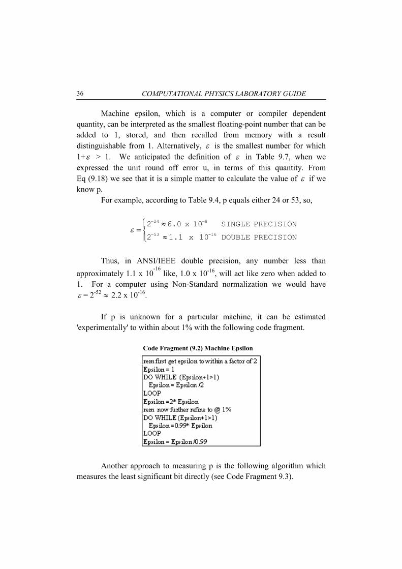
9.8 MACHINE EPSILON/UNIT ROUNDING ERROR By now it should be obvious that the accuracy with which floating-

point numbers can be represented will depend in general on the number of mantissa bits p, and in particular, on the value of the least significant bit. The value of this least significant bit is called the machine epsilon, and is defined as: Machine Epsilon ≡ ε = 2-p (9.18)


Machine epsilon, which is a computer or compiler dependent quantity, can be interpreted as the smallest floating-point number that can be added to 1, stored, and then recalled from memory with a result distinguishable from 1. Alternatively, ε is the smallest number for which 1+ε > 1. We anticipated the definition of ε in Table 9.7, when we expressed the unit round off error u, in terms of this quantity. From Eq (9.18) we see that it is a simple matter to calculate the value of ε if we know p.

For example, according to Table 9.4, p equals either 24 or 53, so,

ε− −

−

≈= ≈

24 8

53 -16

2 6.0 x 10 SINGLE PRECISION

2 1.1 x 10 DOUBLE PRECISION

Thus, in ANSI/IEEE double precision, any number less than

approximately 1.1 x 10-16 like, 1.0 x 10-16, will act like zero when added to

1. For a computer using Non-Standard normalization we would have ε = 2-52 ≈ 2.2 x 10-16.

If p is unknown for a particular machine, it can be estimated

'experimentally' to within about 1% with the following code fragment. Code Fragment (9.2) Machine Epsilon

Another approach to measuring p is the following algorithm which

measures the least significant bit directly (see Code Fragment 9.3).


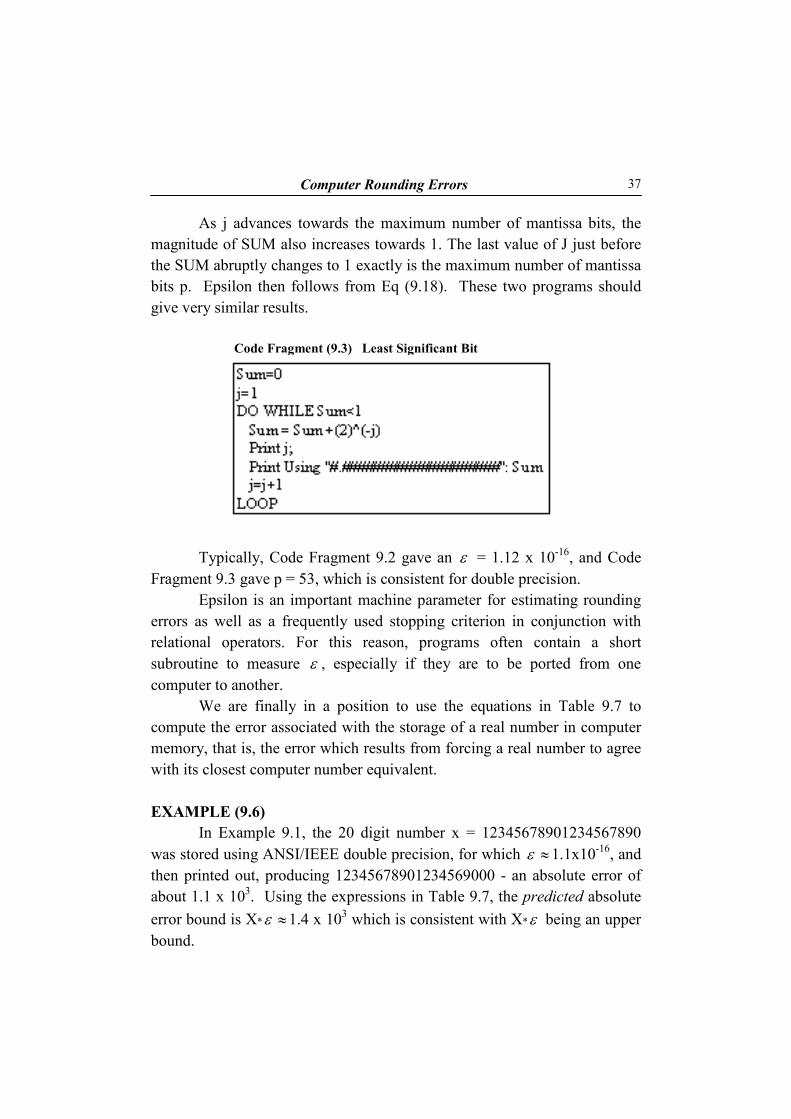
As j advances towards the maximum number of mantissa bits, the magnitude of SUM also increases towards 1. The last value of J just before the SUM abruptly changes to 1 exactly is the maximum number of mantissa bits p. Epsilon then follows from Eq (9.18). These two programs should give very similar results.

Code Fragment (9.3) Least Significant Bit

Typically, Code Fragment 9.2 gave an ε = 1.12 x 10-16, and Code

Fragment 9.3 gave p = 53, which is consistent for double precision. Epsilon is an important machine parameter for estimating rounding

errors as well as a frequently used stopping criterion in conjunction with relational operators. For this reason, programs often contain a short subroutine to measure ε , especially if they are to be ported from one computer to another.

We are finally in a position to use the equations in Table 9.7 to compute the error associated with the storage of a real number in computer memory, that is, the error which results from forcing a real number to agree with its closest computer number equivalent.

EXAMPLE (9.6)

In Example 9.1, the 20 digit number x = 12345678901234567890 was stored using ANSI/IEEE double precision, for which ε ≈1.1x10-16, and then printed out, producing 12345678901234569000 - an absolute error of about 1.1 x 103. Using the expressions in Table 9.7, the predicted absolute error bound is X*ε ≈1.4 x 103 which is consistent with X*ε being an upper bound.


This example illustrates the mechanics of predicting the rounding error associated with the storage of a single real number in computer memory. This result, while interesting, is of limited value unless we are able to expand the concept to include complex arithmetic operations. How this is done is the subject of Chapter 10.

NOTICE - Portland State Universityweb.pdx.edu/~mcclured/Stat Mech/Computer Rounding Error...There...

Documents

Transcript of NOTICE - Portland State Universityweb.pdx.edu/~mcclured/Stat Mech/Computer Rounding Error...There...