Notes V - Heterogeneous Agents & Incomplete Markets · Notes V - Heterogeneous Agents & Incomplete...

Notes V - Heterogeneous Agents & IncompleteMarkets

Julio GarınUniversity of Georgia

Macroeconomic Theory II (Ph.D.)

Spring 2017

Macroeconomic Theory II Notes V - Heterogeneity & Incomplete Markets Spring 2017 1 / 25

Motivation

I Why heterogeneity may be important:

1. Aggregation bias.2. Heterogeneity in decisions and its impact on aggregates.


So Far...

I We have already analyzed heterogeneity:I Equilibrium endowment economy with a complete set of

state-contingent securities.I Also, in some of the extensions of the RBC model.I Heterogeneity “didn’t matter” since idiosyncratic shocks can

be insured away.I Wealth distribution has no impact on aggregate dynamics.

I These models are useful but we cannot study distributionalissues.

I In this sense, complete markets are at odds with the data.I We will have to depart from them.


These Lectures

I We will assume that there is not a complete set ofstage-contingent securities.

I Incomplete-markets model.

I With aggregate shocks, this leads to important computationaldifficulties.

I To simplify, we will consider:I Only idiosyncratic shocks with exogenous restrictions on

available assets.

I Agents will be ex ante homogenous.I But they cannot insure away all idiosyncratic risk.

I They are ex post heterogeneous.


Why is This Difficult?

I In the models so far the Welfare theorems apply.I First best could be achieved by a competitive equilibrium.

I Solving the Social Planner allocation was enough.

I With incomplete markets this is not the case.I We need to solve the competitive equilibrium.

I This, among other things, requires solving for prices.

I Dynamics and uncertainty will be different for individuals andthe aggregate economy.

I With heterogeneous agents, the distribution of asset holdingsis non-degenerate.

I It becomes a state variable.I And it is an infinite object.


Preliminaries: Self-Insurance


Precautionary Motive and Buffer Stock

I With quadratic preferences nothing “bad” happens whenconsumption goes very low.

I With non-quadratic preferences, we will have a relevant thirdmoment:

I U′′′> 0 known as “prudence”.

I Curvature of the marginal utility function.

I Prudence is a motive for additional savings:I Precautionary motive or self-insure.

I Consumption is expected to grow even if ρ = r .

I If ρ > r agents accumulate a “buffer stock” until precautionarymotive is dominated by the agent’s relative impatience.

I Why would we like to focus on this case?


Borrowing Constraints

I Two types of borrowing limits:1. Natural borrowing constraint.

I The constraint self-imposed by the agent.

2. Ad-hoc.

I Ad-hoc constraints are more stringent.I With prudence, a natural borrowing constraint will never bind.

I Ad hoc borrowing constraints will change our previous result:I There will be precautionary savings with quadratic utility.


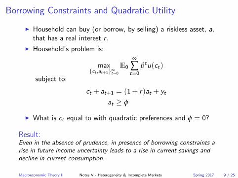
Borrowing Constraints and Quadratic Utility

I Household can buy (or borrow, by selling) a riskless asset, a,that has a real interest r .

I Household’s problem is:

max{ct ,at+1}∞

t=0

E0

∞

∑t=0

βtu(ct)

subject to:

ct + at+1 = (1 + r)at + yt

at ≥ φ

I What is ct equal to with quadratic preferences and φ = 0?

Result:Even in the absence of prudence, in presence of borrowing constraints arise in future income uncertainty leads to a rise in current savings anddecline in current consumption.


Inspecting the Mechanism

I In the previous problem define “cash in hand”, xt , as

xt = (1 + r)at + yt

I Assuming yt is i.i.d., we can then write the problem as:

V (xt) = maxct ,xt+1

u(ct) +1

1 + ρEt V (xt+1)

subject to:

xt+1 = (1 + r)(xt − ct) + yt+1

xt − ct ≥ φ

I The borrowing constraint adds convexity to the problem.I The buffer stock saving with quadratic utility is driven by the

ad hoc constraint.


Heterogeneous Agents Models


Bewley-Aiyagari Models

I Earlier models:I Bewley (1977).I Imrohoroglu (1989).

I GE:I Huggett (1993).I Aiyagari (1994).I Krussell and Smith (1998).


Heterogeneous Agents Models

I We get away from the representative agent model.I We will assume incomplete markets.

I To simplify: we rule out state-contingent securities completely.

I We will cover two versions of Bewley models:

1. Huggett (1993): Endowment economy with bonds in zero netsupply.

2. Aiyagari (1994): Production economy.


Households’ Problem

I There is a unit measure of infinitely-lived households solving:

max{ct ,at+1∈A}∞

t=0

E0

∞

∑t=0

u(ct)

subject to:

ct + at+1 = (1 + r)at + w · sta0 given

I st can be interpreted as the worker’s labor effort.I m-state Markov process with values given by vector s and

transition matrix P .I Model’s source of uncertainty.

I Notice that at+1 is constrained to be on a grid.I There is a borrowing limit.

Back to Aiyagari’s.


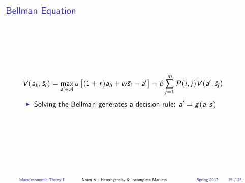
Bellman Equation

V (ah, si ) = maxa′∈A

u[(1 + r)ah + wsi − a′

]+ β

m

∑j=1

P(i , j)V (a′, sj )

I Solving the Bellman generates a decision rule: a′ = g(a, s)


Wealth-Employment Distributions

I Define unconditional distribution of (at , st) pairs:

λt(a, s) = Pr(at = a, st = s)

I With our assumptions, this gives us the distribution of agentsover the state space.

I The law of motion for this distribution is:

λt+1(a′, s ′) =

m

∑j=1

n

∑i=1

Pr(at = ai , st = sj ) · Pr(st+1 = s ′|st = sj )

· Pr(at+1 = a′|at = ai , st = sj )

=m

∑j=1

n

∑i=1

λt(ai , sj ) · Pr(st+1 = s ′|st = sj ) · I(a′|ai , sj )

=m

∑j=1

∑{i :a′=g (ai ,sj )}

λt(ai , sj ) · Pr(st+1 = s ′|st = sj )


I The law of motion depends on:

1. g(a, s).2. P .

I We can calculate an invariant distribution.I About λ.

I The cross-section distribution of agents remains constant.I For a given r the population mean

E(a)(r) = ∑a,s

λ(a, s)g(a, s)

Can be interpreted in two ways:

1. Across-time.2. Across households.


Huggett’s “Pure Credit” Model

I Huggett (1993).I Pure exchange economy.

I Model is closed out by assuming that the bonds are in zero netsupply.

I There is a lower bound on assets given by ai = −φ.

I Interest rate, r , will adjust to equate borrowing and lending.

I Wages are still set exogenously.


Equilibrium in the Huggett Model

Definition (Stationary Equilibrium)

Given φ, a stationary equilibrium is an interest rate r , a policyfunction g(a, s), and a stationary distribution λ(a, s) for which

1. The policy function g(a, s) solves the household’soptimization problem;

2. The stationary distribution λ(a, s) is induced by the (P , s)and g(a, s), satisfying

λ(a′, s ′) =m

∑j=1

∑{i :a′=g (ai ,sj )}

Prob(s ′|s = sj ) · λ(ai , sj )

3. The loan market clears:

∑a,s

λ(a, s)g(a, s) = 0


Huggett’s Equilibrium Computation

1. Fix r = rj for j = 0.

2. Solve household’s problem for gj (a, s).

3. Calculate associated λj (a, s).

4. Compute

∑a,s

λ(a, s)g(a, s) = e∗j

5. If e∗j > 0, lower r .

6. Forward to j + 1 and repeat until e∗j = 0


Aiyagari’s Production Economy

I Aiyagari (1994).I Households now save by buying capital.

I Call it k instead of a.

I Representative firm pays:I r for the rental rate of capital.I w for the households’ labor effort.

I Capital depreciates at δ.I Could be mapped into baseline model. Baseline


Equilibrium in the Aiyagari ModelDefinition (Stationary Equilibrium)A stationary equilibrium is a decision rule g(k, s), a probability distributionλ(k, s), a rental rate r , a wage w , a capital stock K , and an aggregatequantity of labor N such that

1. The policy function g(k, s) solves the household’s optimization problemwith the return on capital given by r = r − δ;

2. The stationary distribution λ(a, s) is induced by (P , s) and g(a, s),satisfying

λ(k ′, s ′) =m

∑j=1

n

∑{i :k ′=g (ki ,sj )}

Prob(s ′|s = sj ) · λ(ki , sj )

3. The aggregate factors of production are given by

K = ∑k,s

λ(k, s)g(k, s)

N = ξ ′∞ s

where ξ∞ is the invariant distribution associated with (P , s);

4. The prices satisfy

w = FN (K ,N) and r = FK (K ,N)− δ


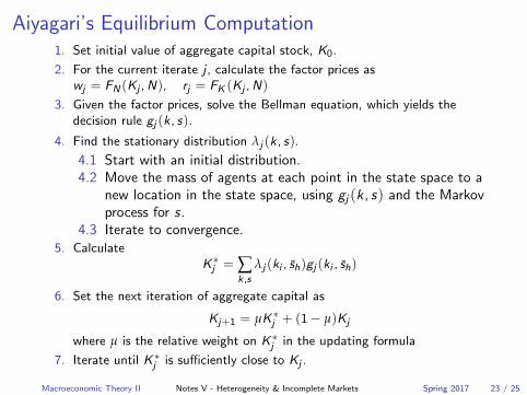
Aiyagari’s Equilibrium Computation1. Set initial value of aggregate capital stock, K0.

2. For the current iterate j , calculate the factor prices aswj = FN (Kj ,N), rj = FK (Kj ,N)

3. Given the factor prices, solve the Bellman equation, which yields thedecision rule gj (k, s).

4. Find the stationary distribution λj (k, s).

4.1 Start with an initial distribution.4.2 Move the mass of agents at each point in the state space to a

new location in the state space, using gj (k , s) and the Markovprocess for s.

4.3 Iterate to convergence.5. Calculate

K ∗j = ∑k,s

λj (ki , sh)gj (ki , sh)

6. Set the next iteration of aggregate capital as

Kj+1 = µK ∗j + (1− µ)Kj

where µ is the relative weight on K ∗j in the updating formula

7. Iterate until K ∗j is sufficiently close to Kj .


Additional Comments

I We can represent both models into a unified diagram.I Where is the buffer stock?I What are the effects of relaxing the constraint?I Capital is higher under incomplete markets.

I What about welfare?

I How can we think about the lower bound of the grid?


Heterogeneous Agent’s With Aggregate Risk

I There will no longer be a stationary distribution.I Stationary equilibrium can no longer be the solution concept.

I The distribution λt(k , s) also becomes part of the statespace.

I Agents need to know that to forecast future factor prices.I Curse of dimensionality.

I Krusell and Smith (1998) propose a computational approach.


Notes V - Heterogeneous Agents & Incomplete Markets · Notes V - Heterogeneous Agents & Incomplete...

Documents

Transcript of Notes V - Heterogeneous Agents & Incomplete Markets · Notes V - Heterogeneous Agents & Incomplete...