Notes on Thermodynamics and Statistical Mechanics
98
Transcript of Notes on Thermodynamics and Statistical Mechanics

Contents
1 Arrows of time and time-reversal symmetry 5
1.1 Arrows of time . . . . . . . . . . . . . . . . . . . . . . . . . . 51.2 Time-Reversal Operations . . . . . . . . . . . . . . . . . . . . 5
1.2.1 Ex. 1. Classical particle . . . . . . . . . . . . . . . . . 61.2.2 Ex. 2 EM . . . . . . . . . . . . . . . . . . . . . . . . . 61.2.3 Ex. 3. QM . . . . . . . . . . . . . . . . . . . . . . . . 7
1.3 Time-Reversal Invariance of dynamical laws . . . . . . . . . . 81.3.1 Example. Newtonian mechanics. . . . . . . . . . . . . . 81.3.2 EM . . . . . . . . . . . . . . . . . . . . . . . . . . . . . 91.3.3 Example. QM . . . . . . . . . . . . . . . . . . . . . . . 91.3.4 Example. Weak-force interactions . . . . . . . . . . . . 10
1.4 Is Time-Reversal Invariance Trivial? . . . . . . . . . . . . . . . 10
2 Basic Concepts and Laws of Thermodynamics 14
2.-1 The Minus First Law and Thermodynamic Equilibrium . . . . 142.0 The Zeroth Law of Thermodynamics . . . . . . . . . . . . . . 15
2.0.1 Ideal gases and thermometry . . . . . . . . . . . . . . . 152.1 The First Law: Heat and Work . . . . . . . . . . . . . . . . . 17
2.1.1 Heat capacity . . . . . . . . . . . . . . . . . . . . . . . 182.2 The 2nd law and Entropy . . . . . . . . . . . . . . . . . . . . 19
2.2.1 Quasistatic, reversible processes . . . . . . . . . . . . . 192.2.2 Work done on a gas . . . . . . . . . . . . . . . . . . . . 202.2.3 Relations between heat capacities . . . . . . . . . . . . 202.2.4 A useful relation . . . . . . . . . . . . . . . . . . . . . 212.2.5 Carnot's theorem . . . . . . . . . . . . . . . . . . . . . 222.2.6 Thermodynamic Temperature . . . . . . . . . . . . . . 232.2.7 The Carnot cycle . . . . . . . . . . . . . . . . . . . . . 24
2.3 Enter Entropy . . . . . . . . . . . . . . . . . . . . . . . . . . . 262.4 Entropy of an ideal gas . . . . . . . . . . . . . . . . . . . . . . 27
2.4.1 Two Examples . . . . . . . . . . . . . . . . . . . . . . . 282.5 Helmholtz Free Energy . . . . . . . . . . . . . . . . . . . . . . 30
3 Kinetic Theory and Reduction 31
3.1 Principle Theories and Constructive Theories . . . . . . . . . 313.2 Elementary Kinetic Theory of Gases . . . . . . . . . . . . . . 32
3.2.1 Heat capacity of a monatomic ideal gas . . . . . . . . . 34
2

4 The Second Law Revised 36
4.1 Tensions between thermodynamics and kinetic theory . . . . . 364.2 The Reversibility Argument . . . . . . . . . . . . . . . . . . . 374.3 The Maxwellian View . . . . . . . . . . . . . . . . . . . . . . . 39
4.3.1 A Third Second Law . . . . . . . . . . . . . . . . . . . 394.3.2 Maxwell on thermodynamics . . . . . . . . . . . . . . . 41
4.4 Exorcising Maxwell's Demon . . . . . . . . . . . . . . . . . . . 43
5 The Boltzmann H-theorem and its discontents 45
5.1 The Ehrenfest wind-tree model . . . . . . . . . . . . . . . . . 455.1.1 The wind-tree H-theorem . . . . . . . . . . . . . . . . 475.1.2 Explicit solution for wind-tree model . . . . . . . . . . 49
5.2 Boltzmann's H-theorem . . . . . . . . . . . . . . . . . . . . . 495.3 The signicance of H . . . . . . . . . . . . . . . . . . . . . . . 51
5.3.1 Wind-tree H . . . . . . . . . . . . . . . . . . . . . . . 515.3.2 Boltzmann's H and Boltzmann's entropy . . . . . . . . 525.3.3 Boltzmann entropy of an ideal gas . . . . . . . . . . . . 545.3.4 Gibbs' paradox . . . . . . . . . . . . . . . . . . . . . . 56
6 Probability 58
6.1 Enter Probability . . . . . . . . . . . . . . . . . . . . . . . . . 586.2 Probability: chance and credence . . . . . . . . . . . . . . . . 59
6.2.1 Axioms of probability . . . . . . . . . . . . . . . . . . . 596.2.2 Conditional probability . . . . . . . . . . . . . . . . . . 596.2.3 Distinct senses of probability . . . . . . . . . . . . . . 606.2.4 Evidence about chances . . . . . . . . . . . . . . . . . 60
6.3 Frequentism . . . . . . . . . . . . . . . . . . . . . . . . . . . . 626.4 Classical Probability and Symmetries . . . . . . . . . . . . . . 63
6.4.1 Knowledge from ignorance? . . . . . . . . . . . . . . . 656.5 Measure spaces and measures . . . . . . . . . . . . . . . . . . 666.6 Probability ow; Liouville's theorem . . . . . . . . . . . . . . 67
7 Probabilities in Statistical Mechanics 69
7.1 The brute posit. . . . . . . . . . . . . . . . . . . . . . . . . . . 697.2 Appeals to typicality . . . . . . . . . . . . . . . . . . . . . . . 717.3 The Ergodic Hypothesis . . . . . . . . . . . . . . . . . . . . . 727.4 Boltzmann-Schuetz cosmology . . . . . . . . . . . . . . . . . . 757.5 Almost-objective probabilities . . . . . . . . . . . . . . . . . . 77
3

7.6 Probabilities from quantum mechanics? . . . . . . . . . . . . . 807.7 Return of the Stoÿzahlansatz? . . . . . . . . . . . . . . . . . . 82
7.7.1 Is the Stoÿzahlansatz justied? . . . . . . . . . . . . . 82
8 Gibbs entropy 84
8.1 Canonical distribution and entropy . . . . . . . . . . . . . . . 848.2 Properties of the Gibbs entropy . . . . . . . . . . . . . . . . . 868.3 Gibbs on Thermodynamic Analogies . . . . . . . . . . . . . . 87
8.3.1 Gibbs entropy and Boltzmann entropy compared . . . 88
4

1 Arrows of time and time-reversal symmetry
1.1 Arrows of time
Intuitively, there are many sorts of dierence between the future-pointingdirection of time, and the past-pointing direction. Consider
• Psychological. We remember the past, anticipate the future. There isalso alleged to be a `feeling of the passage of time.'
• Biological. We biological organisms go through life stages in a determi-nate order: conception (or birth by ssion), embryo, youth, maturity,senescence, death.
• Thermodynamic. The laws of thermodynamics are not invariant undertime reversal. Typically it is the Second Law that is said to be theculprit.
• Radiative. EM radiation is commonly found radiating outward fromstars, light bulbs, burning matches, etc. Much more rarely, if at all, dowe nd spherical waves converging on an object and being absorbed byit.
• Causal. A cause comes before an eect, not vice versa.
• Humpty Dumpty. You can't unscramble an egg.
This is not meant to be an exhaustive list. Nor are the items in the listindependent of each other; there seem to be interesting relations betweenthem. An attractive position is that all of these are reducible to one of them(think about how this might work).
One position that has been defended is that temporal asymmetries areonly apparent; to beings like us, with a temporally asymmetric perspectiveon the world, there seems to be a distinction in the physical world. I don'tbuy it, but see Price (1996) for an extended defense of this view.
1.2 Time-Reversal Operations
A physical theory, typically, represents the state of a system by a point insome state space Ω.
5

• The state of a single classical particle is represented by its positionand momentum (x,p), which can be thought of as a point in its 6-dimensional phase space.
• The state of n classical particles is represented by a point in a 6n-dimensional phase space.
• The state of a quantum system is represented by a vector in a complexHilbert space.
• The thermodynamic state of a system is given by a small (compared tothe dimension of the phase space of all the particles that make up thesystem) number of macroscopically measurable parameters.
A state history is a trajectory through phase space; that is, a mappingσ : I ⊆ R→ Ω, for some time interval I.
A physical theory will also typically include a set of dynamical laws thatdistinguish, from among the kinematically possible trajectories, a set D ofdynamically possible trajectories.
Given any time t0, we can dene a reection of the time axis around t0by
t→ tT = t0 − (t− t0) (1.1)
It's traditional to take t0 = 0, so that tT = −t.We can also talk about time-reversal of states.
1.2.1 Ex. 1. Classical particle
For a classical particle, the operation of time-reversal is (perhaps obviously)
(x,p)→ (x,−p). (1.2)
1.2.2 Ex. 2 EM
In electromagnetic theory the standard view of time-reversal has chargesremaining invariant, velocities (and hence currents) changing sign.
ρ→ ρJ→ −J, (1.3)
with elds going as
6

E→ EB→ −B (1.4)
There is a heterodox view, on which the time-reversal operation should leaveboth electric and magnetic elds invariant. See Albert (2000). For anotherheterodox view, on which time-reversal operation ips the sign of charges aswell, see Arntzenius and Greaves (2007) and Leeds (2006).
For two, somewhat dierent, defenses of the orthodox view, see Earman(2002) and Malament (2004).
1.2.3 Ex. 3. QM
In quantum mechanics, the state of a spinless particle is represented by awave-function ψ.
To see how to time-reverse this, consider the following:
1. By Wigner's theorem,1 there exists a either a unitary transformationor an antiunitary transformation that implements the operation.
2. We want
(a) 〈x〉 → 〈x〉(b) 〈p〉 → −〈p〉
This yields the result that the wave function's transformation under timereversal is given by the anti-unitary transformation
ψ → ψ∗. (1.5)
When spin is to be taken into account, the time-reversal operator is de-ned so as to ip the signs of spins. (Rationale: spin, being a form of angularmomentum, should change sign, just as orbital angular momentum does.)
For a heterodox view, according to which time-reversal should leave ψunchanged, see Callender (2000).
1See Weinberg (1995, Ch. 2, Appendix A) for an exposition.
7

1.3 Time-Reversal Invariance of dynamical laws
.We are now ready to consider time-reversal invariance of physical laws.Given a time-reection
t→ tT = t0 − (t− t0) (1.6)
and a state-reversal operation
ω → ωT , (1.7)
we can dene an operation that reverses state histories. Dene the history-reversal operation
σ → σT (1.8)
byσT (t) = σ(tT )T . (1.9)
So, if σ includes a sequence of states ...σ(t1), σ(t2), σ(t3)..., then the time-reversed history includes a sequence of states ...σ(tT3 )T , σ(tT2 )T , σ(tT1 )T , ....
We say that a physical theory is time-reversal invariant i, whenever astate history σ is dynamically possible, the time-reversed state history σT istoo. Or, in other words, the theory is time-reversal invariant i DT ⊆ D.
1.3.1 Example. Newtonian mechanics.
Suppose we have a system of n Newtonian particles. Newton's 2nd law saysthat
mid2xidt2
= Fi, (1.10)
where Fi is the total force on the ith particle.Given a system of Newtonian particles, suppose that the force on any one
of the particles depends only on the positions of the particles.
Fi = Fi(x1, ...,xn). (1.11)
Then both left and right-hand sides of Equation (1.10) remain unchangedunder time-reversal, and so the law of motion is time-reversal invariant.
8

If, however, the force depends on velocity, then we will not have time-reversal invariance. Consider, e.g. a damped harmonic oscillator, whoseequation of motion is
m x = −kx− bx. (1.12)
If x(t) is a solution to this equation, then, except for the trivial (equilib-rium) solution x(t) = 0, its time reversal will not be a solution. Solutionsto Equation (1.12) are oscillations with exponentially decreasing amplitude(assuming subcritical damping). The time-reverse of such a solution wouldbe an oscillation with exponentially increasing amplitude.
(To ponder: in damping, what is going on at the microphysical level?)
1.3.2 EM
Maxwell's equations are
∇ · E = 4πρ ∇× E + 1c∂B∂t
= 0
∇ ·B = 0 ∇×B− 1c∂E∂t
= 4πcJ
(1.13)
Under time reversal
∇ → ∇t → −tρ → ρ
J → −J,E → E
B → −B
And so we have TRI.
1.3.3 Example. QM
The law of motion is the Schrödinger equation:
i~∂
∂tΨ = HΨ. (1.14)
Suppose the Hamiltonian for a particle takes the form:
H = − ~2
2m∇2 + V (x). (1.15)
9

Then, if Ψ(x, t) satises the S. eq., then ΨT (x, t) = Ψ(x,−t)∗ satises
−i~ ∂
∂tΨT = HΨT , (1.16)
or,
i~∂
∂tTΨT = HΨT , (1.17)
which is the time-reversed Schrödinger equation. So QM is TRI providedthat the Hamiltonian is invariant under time-reversal.
1.3.4 Example. Weak-force interactions
At this point, you may be forming the induction: physical laws are, at thefundamental level, time-reversal invariant, and perhaps conjecturing that, fordeep reasons, theymust be. Before dashing o an a priori proof of this, pauseto consider: there is evidence that interactions involving the weak nuclearforce are not TRI. Indirect evidence of this rst came through evidence of CPviolation; by the CPT theorem, the same processes must involve T-violation.The rst direct evidence of violation of T-symmetry, involving neutral kaondecays, was reported in Angelopoulos et al. (1998). T-violation has also beenrecently observed in the B-meson system (Lees et al., 2012).
Thus, it can't be a metaphysical necessity that the laws of physics areTRI. However, there are principled reasons for regarding these violations oftime reversal invariance as irrelevant to the temporal asymmetries associatedwith thermodynamics. One way to see this is that, although the laws ofnature are invariant under time reversal, there is good reason to think (asthis follows from Lorentz invariance) that they are invariant under CPT: theoperation that combines charge conjugation (particle→ antiparticle), parity(that is, mirror) reection, and time reversal. Unless a gas consisting of anti-hydrogen molecules exhibits anti-thermodynamic behaviour, the temporalasymmetries of thermodynamics are also violations of CPT symmetry.2
1.4 Is Time-Reversal Invariance Trivial?
If you take a look at textbook accounts of the treatment of time-reversaloperations in EM, or in QM, they fall into two classes. There are those thatjustify the standard time-reversal operation on the grounds that it is what it
2This point has been made by Price (2006).
10

takes to make the theory TRI, and those that attempt to give an independentrationale for the operation. The former strategy engenders the suspicion thatwe are cooking up the time-reversal operation to save a symmetry that wehappen to like. This charge has been laid, for EM, by Albert (2000), chapter1, and, for QM, by Callender (2000). And one distinguished author hasargued that, for any deterministic theory, it is possible to cook up a timereversal operation that the theory is TRI.
If one were to allow completely arbitrary time reversal operations,then any deterministic theory would count as time reversible. Forexample, take some particular state history S(t) that is possibleaccording to the theory. Let us now dene what the time inverseST is of any state that lies on that particular history. Begin byarbitrarily choosing some time t0. Then declare that the timereversal of the state S(t0 + δt) that occurs a period of time δtafter t0 is, in fact, the state that occurs time period δt before t0,i.e., S(t0 − δt).... given any deterministic theory one can dene a time rever-sal operation T that shows that the theory in question is timereversible. But that is absurd. (Arntzenius, 2004, 3233)
Arntzenius is right that it is absurd. But it's worthwhile to think aboutwhy it's absurd. (How would this sort of time reversal operation lookwhen applied to, say, a damped harmonic oscillator, which exhibits observabletemporal asymmetry?)
A theory that exhibits temporal asymmetry at the level of observablephenomena is clearly not a candidate for a theory that is TRI. Suppose, then,that the observable phenomena do not pick out a distinguished direction oftime for any sequence of observations, the reversed sequence is possible,according to the theory. (Remember, we do not observe EM elds directly,but only through their eects on charged particles). If, now, we held apositivist view, according to which the observable consequences of a theoryexhaust its physical content, and any apparent reference to structure thatis not directly observable merely `dressing' of the real content of the theory,we'd be done, and declare the theory TRI. There are good reasons (beyondthe scope of this course) for not adopting such a narrow view of the content ofa theory. However, if, according the theory, the phenomena fail to distinguishtemporal orientations, this at least suggests that the theory is TRI, and that
11

apparent temporal asymmetries in our theoretical treatment are artifactsof our representation. We ought, therefore, to ask ourselves whether, byreecting on the physical signicance of the part of the theory that refersto structures that are not directly observable, we will conclude that theappropriate time-reversal operation shows the theory to be TRI.
That is, we are imagining something analogous to Einstein's train ofthought in his 1905 paper, On the Electrodynamics of Moving Bodies.Einstein begins with the observation that electromagnetic phenomena de-pend, not on the absolute motions of the systems involved, but only on theirrelative motions. Our theoretical description, on the other hand, introducesan asymmetry that is not present in the phenomena. This at least suggeststhat the asymmetry is an artifact of our representation. Einstein then showsthat it is possible to formulate the theory in a way that does not distin-guish between states of inertial motion; on this formulation the partitionof the electromagnetic force on a charged body into electrical and magneticcomponents is explicitly a frame-relative matter.
Malament (2004) does something analogous for time reversal in EM. Ifwe consider a system of charges moving under the inuence of electromag-netic forces, their behaviour does not distinguish between past and futuredirections of time. This suggests that we try to formulate the theory in away that does not distinguish the two directions. The key to how to do thiscomes from the following remark:
We can think of it [the EM eld tensor] as coding, for everypoint in spacetime, the electromagnetic force that would be ex-perienced by a point test particle there, depending on its chargeand instantaneous velocity.
Malament shows that it is, in fact, possible to provide a coordinate-freerepresentation of the theory that does not require a temporal orientation that is, does not require us to declare which of the two temporal direction ispast, and which is future. It turns out that, on this formulation, componentsof the electromagnetic eld tensor are dened only given a choice of tem-poral orientation and handedness of spatial coordinate system. Malament'streatment leads naturally to the conclusion that, under temporal inversion,
E→ EB→ −B. (1.18)
12

The upshot of the analysis is that the magnetic eld is represented by anaxial vector.
The transformation properties for Ba are exactly the same as forangular velocity. ... Magnetic eld might not be rates of changeof anything in the appropriate sense, but they are axial vectorelds (Malament, 2004, 313314).
This is not news; Maxwell already knew this!
The consideration of the action of magnetism on polarized lightleads, as we have seen, to the conclusion that in a medium undermagnetic force something belonging to the same mathematicalclass as an angular velocity, whose axis in the direction of themagnetic force, forms a part of the phenomenon. (Maxwell, 1954,822).
Maxwell went on to argue that magnetic elds were, in fact, associatedwith vortices in the electromagnetic ether. We have abandoned the ether, butthe conclusion that magnetic elds transform, under parity and time reversal,in the same way that an angular velocity does, survives the abandonment.
13

2 Basic Concepts and Laws of Thermodynam-
ics
Early writers on thermodynamics tended to talk of two fundamental lawsof thermodynamics, which came to be known as the First and Second Lawsof Thermodynamics. However, another law has been recognized, regardedas more fundamental than the rst two, which has accordingly come to beknown as the Zeroth Law. But perhaps there is also a Minus First Law, morefundamental than all of these (see Brown and Unk (2001) for extendeddiscussion). There is also a Third Law of Thermodynamics (which, thoughimportant, will play less of a role in our discussions).
2.-1 The Minus First Law and Thermodynamic Equi-
librium
Thermodynamicists get very excited, or at least get very inter-ested, when nothing happens... . (Atkins, 2007, p. 7)
On the rst page of Pauli's lectures on thermodynamics we nd,
Experiment shows that if a system is closed, then heat is ex-changed within the system until a stable thermal state is reached;this state is known as thermodynamic equilibrium. (Pauli, 1973,p. 1)
Similar statements can be found in the writings of others, and, even whennot explicitly stated, it is taken for granted. Brown and Unk have dubbedthis the Minus First Law, or Equilibrium Principle, which they state as,
An isolated system in an arbitrary initial state within a nite xed
volume will spontaneously attain a unique state of equilibrium.
(Brown and Unk, 2001, p. 528)
Note that this is a time-asymmetric law. Once an isolated system attainsequilibrium, it never leaves it without outside intervention; the time reversalof this is not true. Brown and Unk argue that it is this law, not, as mostwriters on the subject would have it, the Second, that is at the heart of thetime asymmetry of thermodynamics.
It is interesting that time asymmetry is present in what is perhaps themost fundamental concept of thermodynamics, that of equilibrium.
14

2.0 The Zeroth Law of Thermodynamics
The concept of thermodynamic equilibrium can be used to introduce theconcept of temperature. Two bodies that are in thermal contact (this meansthat heat ow between them is possible), which are in thermal equilibriumwith each other, will be said to have the same temperature. We want thisrelation of equitemperature to be an equivalence relation. It is reexive andsymmetric by construction. That it is transitive is a substantive assumption3
(though one that has often been taken for granted). Suppose we have bodiesthat can be moved around and brought into thermal contact with each other.When this happens, the contact might induce a change of state (brought onby heat transfer from one to the other), or it might not. The zeroth law saysthat, if two bodies A, B are in equilibrium with each other when in thermalcontact, and B and C are in equilibrium with each other, then A and C arein equilibrium with each other.
2.0.1 Ideal gases and thermometry
A recurring example we will use will be ideal gases. An ideal gas has a par-ticularly simple thermodynamic state space: its equilibrium thermodynamicstates are determined by the pressure, temperature and volume of the gas,and, because these are related by the equation of state, there are only twoindependent parameters, so we have a two-dimensional state space.
An ideal gas is dened to be one satisfying
• Boyle's Law. At xed temperature,
p ∝ 1
V. (2.1)
• Joule's Law. The internal energy depends only on the temperature.
Note that these depend only on the notion of same temperature, intro-duced on the basis of the 0th Law. Both of these are obeyed to a goodapproximation by real gases, provided that the density is not too high.
Before we can write the equation of state down, we need to introduce atemperature scale.
Boyle's law entails that there is a function of the thermodynamic state ofthe gas, call it θ ∝ pV , that takes on the same value at equal temperatures
3Noted and emphasized by, among others, Maxwell; see Maxwell (2001, pp. 3233)
15
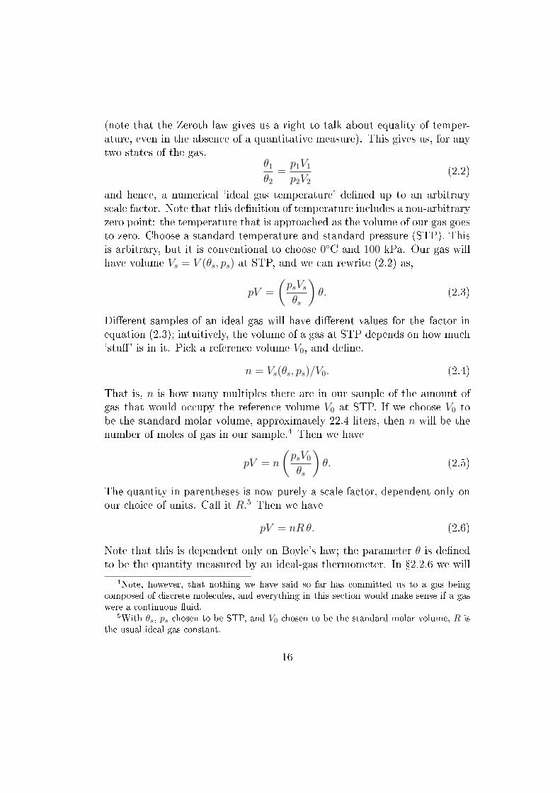
(note that the Zeroth law gives us a right to talk about equality of temper-ature, even in the absence of a quantitative measure). This gives us, for anytwo states of the gas,
θ1
θ2
=p1V1
p2V2
(2.2)
and hence, a numerical `ideal gas temperature' dened up to an arbitraryscale factor. Note that this denition of temperature includes a non-arbitraryzero point: the temperature that is approached as the volume of our gas goesto zero. Choose a standard temperature and standard pressure (STP). Thisis arbitrary, but it is conventional to choose 0C and 100 kPa. Our gas willhave volume Vs = V (θs, ps) at STP, and we can rewrite (2.2) as,
pV =
(psVsθs
)θ. (2.3)
Dierent samples of an ideal gas will have dierent values for the factor inequation (2.3); intuitively, the volume of a gas at STP depends on how much`stu' is in it. Pick a reference volume V0, and dene,
n = Vs(θs, ps)/V0. (2.4)
That is, n is how many multiples there are in our sample of the amount ofgas that would occupy the reference volume V0 at STP. If we choose V0 tobe the standard molar volume, approximately 22.4 liters, then n will be thenumber of moles of gas in our sample.4 Then we have
pV = n
(psV0
θs
)θ. (2.5)
The quantity in parentheses is now purely a scale factor, dependent only onour choice of units. Call it R.5 Then we have
pV = nR θ. (2.6)
Note that this is dependent only on Boyle's law; the parameter θ is denedto be the quantity measured by an ideal-gas thermometer. In 2.2.6 we will
4Note, however, that nothing we have said so far has committed us to a gas beingcomposed of discrete molecules, and everything in this section would make sense if a gaswere a continuous uid.
5With θs, ps chosen to be STP, and V0 chosen to be the standard molar volume, R isthe usual ideal gas constant.
16

introduce, via the Second Law, a notion of thermodynamic temperature T ,which will turn out to be proportional to θ. Choosing equal units for θ andT gives us the ideal gas equation of state in its familiar form,
pV = nRT, (2.7)
which is called the ideal gas law.
2.1 The First Law: Heat and Work
We are used to the idea that energy is conserved. A system of bodies willhave a total internal energy that consists, in part, of the kinetic energy of itscomponents, which may be in motion, and in part, to the potential energydue to the forces acting between them.
One way to add energy to a system is to do work on it. For example,I may compress a spring. The compressed spring has a potential energy,which can be converted to kinetic energy. Or I can lift a weight, whichgains gravitational potential energy, which again can be recovered as kineticenergy. The energy that I can get back out, when I compress an ideal springfrom an initial state Si to a nal state Sf , is equal to
W = −∫ Sf
Si
F · dx, (2.8)
where F is the force opposing my eorts. It is dened this way so that theincrease of energy of the system on which I do work is equal to the work Ido.
Suppose, now, that I expend the same amount of work by, say, stirring aviscous uid, or by rubbing two rough surfaces together. I won't be able torecover as kinetic energy the energy I put in as work at least not all of it.The system I did work on, however, will get warmer. The energy I expendeddid not vanish; it was converted into heat.
Here, again, it might seem like we're cheating. Every time there's anapparent violation of conservation of energy, we invent a new form of energy rst potential energy, and then heat to compensate for the apparentlylost energy. This might make the principle of conservation of energy seemto be an empty one with enough imagination, it might seem, we couldcome up with a new form of energy to make energy conservation true, nomatter what happens. However, what gives the notion some teeth is the fact
17

that there is a measurable mechanical equivalent of heat : we can measurethe amount of work it requires to raise, say, a gram of water 1 degree.
The First Law of Thermodynamics says that, if an amount of work Wis done on a system, and heat Q passes into it, the internal energy U of thesystem is changed by an amount
∆U = Q+W (2.9)
Note: the terms work and heat are used in connection with two modes ofenergy transfer. I can do work on a system, and transfer energy to it thatway. Energy can also be transferred as heat ow between two bodies inthermal contact. We're tempted to think of heat as a substance that canow from one body to another (indeed, this was at one time a theory thatwas taken seriously), but on the modern view, energy transferred as workcan be extracted as heat, and vice versa, and it makes no sense to talk aboutthe heat content of a body.
We will often want to integrate the change of internal energy along someprocess. For that reason, the dierential form of the First Law will frequentlybe more useful.
dU = d Q+ dW (2.10)
Writing `dU ' indicates that the quantity is a change in a function of state:some quantity that depends only on the thermodynamic state of the system.As mentioned above, we do not ascribe to a body some quantity Q thatrepresents the heat it contains. The small heat transferred is not a changein a state function, and we write it as `d Q' to signal this. We call a quantitysuch as dU , that is a change in a state function, an exact dierential, and aquantity, such as d Q or dW , that is not a change in a state function, andinexact dierential.
A bit of jargon: a system is adiabatically isolated i it can't exchange heatwith the environment, and an adiabatic process is one in which the systemexchanges no heat with the environment.
2.1.1 Heat capacity
Dene the constant-volume heat capacity of a gas as the amount of heat d Qrequired to raise the temperature by an amount dθ.
CV =
(d Q
dθ
)V
=
(∂U
∂θ
)V
, (2.11)
18

where the subscript V indicates that the heating is being done at constantvolume. We can also heat a gas at constant pressure, say, by allowing it toraise a piston with a weight on it, and dene constant-pressure heat capacityas
Cp =
(d Q
dθ
)p
. (2.12)
In constant-pressure heating, some of the energy I put in goes into raisingthe temperature, and some into expansion (the gas does work on the envi-ronment). We should, therefore, expect that it takes more heat to raise thetemperature of a gas one degree under constant pressure than it does underconstant volume, that is,
Cp > CV . (2.13)
For the quantitative relations between heat capacities, see section 2.2.3,below.
2.2 The 2nd law and Entropy
But by reason of the Tenacity of Fluids, and Attrition of theirParts, and the Weakness of Elasticity in Solids, Motion is moreapt to be lost than got, and is always upon the Decay.
Newton, Opticks (Newton, 1952, p. 398)
2.2.1 Quasistatic, reversible processes
A central distinction in thermodynamics is between two kind of processes. Onthe one hand, there are processes that take place gently, with no churning orturbulence or friction, and which no heat is transferred from a warmer bodyto a colder (all of these things involve lost opportunities to do work with theenergy transferred). On the other hand, there are all other processes.
Example: if I compress a gas, then at minimum I have to exert a forceon the gas that is equal to the opposing pressure. But if the force I exert isexactly the same, nothing happens. However, assuming a frictionless piston,any slight push I make, above and beyond the force needed to hold thepiston in place, will compress the gas, and, provided I am willing to waitlong enough, I can compress the gas using arbitrarily small force beyondthat which counteracts the pressure.
19

The word `quasistatic' is often used in connection with such processes,as is the word `reversible.' A quasistatic process is meant to be one thatis carried out so slowly that, at every moment, the system is eectivelyin equilibrium. Reversibility is meant to indicate that the initial state isrecoverable. If I compress a gas slowly by doing work on it, say, by allowinga spring to extend, then I can get the energy transferred out by allowingthe gas to expand and recompress the spring. Note that `reversible' heredoesn't necessarily mean that the time-reverse of the process is possible. Fora careful discussion of these concepts, see Unk (2001).
What we want are processes that are quasistatic and reversible. I willusually say `qsr.' However, there doesn't seem to be a good adverbial formof this, so I will sometimes say `quasistatically' when what I really mean is,`in a qsr manner.'
2.2.2 Work done on a gas
Suppose we compress a gas quasistatically by an amount dV , by movinga piston of area A a distance dx. Since this is a compression, the volumedecreases.
dV = −Adx (2.14)
The force opposing this compression is due to the pressure exerted by thegas by the piston. Since pressure is force per unit area, the force exerted onthe piston is pA , and the work I do on the has in compressing it is
dW = pAdx = −pdV. (2.15)
Hence, a useful form of the First Law for a gas (or any system that can onlydo work on the outside world by expanding) is that, for any qsr process,
dU = d Q− p dV. (2.16)
2.2.3 Relations between heat capacities
From eq. 2.16 it follows that, for any gas,(∂U
∂θ
)p
=
(d Q
dθ
)p
− p(∂V
∂θ
)p
, (2.17)
and so,
Cp =
(d Q
dθ
)p
=
(∂U
∂θ
)p
+ p
(∂V
dθ
)p
. (2.18)
20

It can also be shown (left as an exercise for the reader), that, for any gas,
Cp − CV =
[p+
(∂U
∂V
)θ
](∂V
∂θ
)p
. (2.19)
Joule's law says that the internal energy of an ideal gas depends only onits temperature, and hence, (
∂U
∂V
)θ
= 0. (2.20)
From the ideal gas law we have,(∂V
∂θ
)p
=nR
p, (2.21)
and so, for an ideal gas,Cp − CV = nR. (2.22)
It is convenient to work with the molar heat capacities cp = Cp/n, cV =CV /n, related by
cp − cV = R. (2.23)
We also dene
γ =CPCV
=cpcV. (2.24)
Note that, given the way we have dened heat capacities, they could,in principle (and for some systems do) vary with the state of the system.However, experience shows that the heat capacity of an ideal gas does notchange with temperature. This, together with Joule's law, gives us,
dU = CV dθ. (2.25)
Since left and right side are state functions, this is true for any change ofstate, whether reversible or not. It also follows that, since the dierencebetween CP and CV is a constant, that CP , and hence γ, is also constant.
2.2.4 A useful relation
For an ideal gas undergoing a qsr, adiabatic process,
dU = CV dθ = −pdV (2.26)
21

From the ideal gas law, p = nRθ/V , and so we have
dθ
θ= −
(R
cv
)dV
V= − (γ − 1)
dV
V. (2.27)
Integrating this gives the conclusion that, for an adiabatic, qsr process
θ V γ−1 = const. (2.28)
2.2.5 Carnot's theorem
Consider a heat engine that absorbs heat Qin from a heat reservoir, doesnet work W on the external world, and discards some waste heat Qout intoanother (cooler) reservoir. (These reservoirs are to be regarded as so largethat they can supply or absorb these quantities of heat with negligible changein temperature.) Suppose, further, that the heat engine operates in a cycle,so that it returns to its original thermodynamic state at the end of the cycle.This means that the engine undergoes no net change in internal energy.Conservation of energy entails
W = Qin −Qout, (2.29)
The engine absorbs heat Qin from the hot reservoir, and converts fraction
η =W
Qin
(2.30)
of it into useful work, and discards the rest. The fraction η is called theeciency of the engine.
η = 1− Qout
Qin
. (2.31)
Carnot's theorem tells us about the maximum eciency of such an engine:
Any two heat engines operating in a qsr manner between two heatreservoirs have the same eciency, which is dependent only onthe temperature of the two reservoirs. Moreover, any other heatengine has lower eciency.
The argument for this is based on the observation that, though heat owsspontaneously from a hot to a cold body, we have to do something e.g.
expend some work to transfer heat from a cold to a hot body. Clausiusexpressed the latter idea by,
22

Heat cannot pass from a colder body to a warmer body withoutsome other change connected with it occurring at the same time.6
This is often called the Clausius statement of the Second Law of Thermody-
namics.
Here's the argument. A given reversible engine Er, run forward, extractsheat from the hot reservoir and converts a portion of it into work. The cyclecan be run backward: If we do work on Er, we can use it to move heat fromthe cold reservoir to the hot; that is, we use it as a refrigerator. Let theeciency of Er be ηr, and let Es be some other engine, with eciency ηs.
Let Es extract an amount of heat QH from the hot reservoir, do workW = ηsQH on Er, and discard heat QC = (1 − ηs)QH . The work done onEr is used to drive it backwards, extracting heat Q′C from the cold reservoir,and dumping heat Q′H into hot reservoir. We have,
W = ηsQH = ηrQ′H , (2.32)
and so, the net result of the cycle is to move a quantity of heat
Q = Q′H −QH =
(ηsηr− 1
)QH (2.33)
from the cold reservoir to the hot reservoir. If ηs > ηr, this is positive, andthe net result of the process was to move heat from the cold reservoir to thehot, which L2 says is impossible. Conclusion:
For engine Es and any reversible engine Er, ηs ≤ ηr.
From which it follows
All reversible engines have the same eciency.
2.2.6 Thermodynamic Temperature
Forget, for the moment, that we have already introduced the ideal gas tem-perature θ. Carnot's theorem tells us that the eciency of a reversible heatengine operating between two reservoirs depends only on their temperature;
6Es kann nie Wärme aus einem kälteren Körper übergehen, wenn nicht gleichzeitigeine andere damit zusammenhängende Aenderung eintritt. Quoted by Unk (2001, p.333).
23

here the notion of `same temperature' that we are helping ourselves to is theequivalence relation underwritten by the Zeroth Law. We can use this factto dene a temperature scale. If ηAB is the eciency of a reversible engineoperating between reservoirs A, B, dene the thermodynamic temperature Tby
TBTA
=df 1− ηAB. (2.34)
This denes the thermodynamic temperature of any reservoir up to an arbi-trary scale factor. With the scale chosen so that degrees are equal in size toCentigrade degrees, this is (of course) called the Kelvin scale.
2.2.7 The Carnot cycle
For the purposes of scientic illustration, and for obtaining clearviews of the dynamical theory of heat, we shall describe the work-ing of an engine of a species entirely imaginaryone which it isimpossible to construct, but very easy to understand.
(Maxwell, 2001, pp. 138139)
We now have two temperature scales on our hands: the ideal gas tem-perature θ, and the thermodynamic temperature T , and we may justly askwhether there is any relation between them. To this end, we will imagine aheat engine whose working substance is an ideal gas, and consider a reversiblecycle that is particularly simple to analyze, get the eciency of this cycle interms of the ideal gas temperature, and hence get a relation between idealgas and thermodynamic temperature scales.
Since transfer of heat between bodies of unequal temperature is an irre-versible process, we will arrange our cycle so that any heat exchange occursat constant temperature, in contact with one of the reservoirs. The cycle willbe broken into four steps:
1. a→ b. Constant temperature expansion at temperature θH . Heat Qin
absorbed by the system from the hot reservoir. Work is done by thegas on the environment.
2. b → c. Adiabatic expansion. The gas does work on the environment,cooling as it does to temperature θC .
24
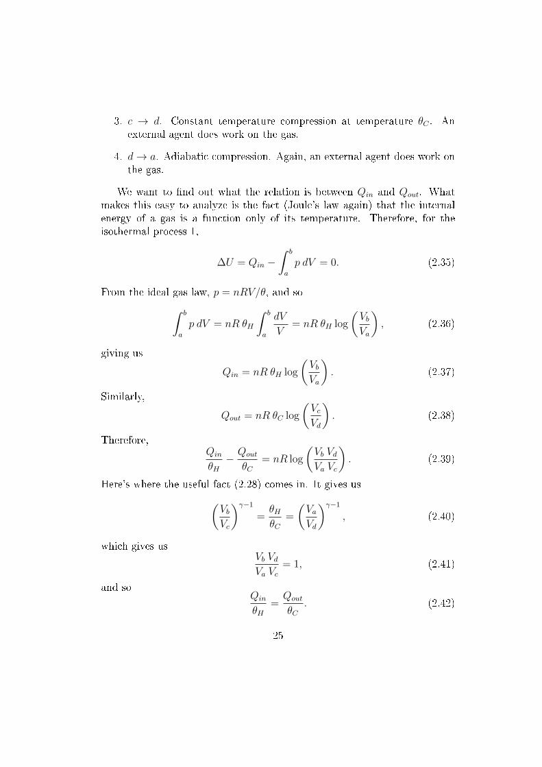
3. c → d. Constant temperature compression at temperature θC . Anexternal agent does work on the gas.
4. d→ a. Adiabatic compression. Again, an external agent does work onthe gas.
We want to nd out what the relation is between Qin and Qout. Whatmakes this easy to analyze is the fact (Joule's law again) that the internalenergy of a gas is a function only of its temperature. Therefore, for theisothermal process 1,
∆U = Qin −∫ b
a
p dV = 0. (2.35)
From the ideal gas law, p = nRV/θ, and so∫ b
a
p dV = nR θH
∫ b
a
dV
V= nR θH log
(VbVa
), (2.36)
giving us
Qin = nR θH log
(VbVa
). (2.37)
Similarly,
Qout = nR θC log
(VcVd
). (2.38)
Therefore,Qin
θH− Qout
θC= nR log
(Vb VdVa Vc
). (2.39)
Here's where the useful fact (2.28) comes in. It gives us(VbVc
)γ−1
=θHθC
=
(VaVd
)γ−1
, (2.40)
which gives usVb VdVa Vc
= 1, (2.41)
and soQin
θH=Qout
θC. (2.42)
25

Therefore, the eciency of the Carnot engine is
ηHC = 1− θCθH. (2.43)
Comparison of (2.34) and (2.43) yields the happy result that
θ ∝ T, (2.44)
and of course, the easiest convention to adopt is to use the same size units foreach, in which case we have equality of θ and T . Henceforth, we will speakonly of T .
2.3 Enter Entropy
Around a Carnot cycle, ∮d Q
T=Qin
TH− Qout
TC= 0. (2.45)
Moreover, this must be true around any qsr cycle in the ideal gas state space.The argument: any cycle in the state space of our system can be approxi-mated as closely as we want by a path that alternates between isothermaland adiabatic segments, and, for such paths, (2.45) holds.
So, we conclude, for any thermodynamic system,∮qsr
d Q
T= 0. (2.46)
Argument: if it didn't hold, we could construct a reversible engine with aneciency dierent from the Carnot eciency, in contravention of Carnot'stheorem.
It follows that there exists a state function S such that, for any qsrprocess, ∫ b
a
d Q
T= Sb − Sa, (2.47)
or, in dierential form,
dS =
(d Q
T
)qsr
. (2.48)
26

This state function is called the thermodynamic entropy of the system. Notethat it is dened only up to an arbitrary additive constant; it is entropydierences between thermodynamic states that are physically signicant.
A heat engine operating between two reservoirs that is less ecient thana Carnot engine will have
Qout
Qin
>TCTH
, (2.49)
hence, for the cycle of such an engine,∮d Q
T< 0. (2.50)
We can express the content of (2.45) & (2.50) in dierential form: for anyprocess,
d Q ≤ T dS, (2.51)
with equality holding for reversible processes. It follows that, for an adia-batically isolated system, which cannot exchange heat with the rest of theworld,
dS ≥ 0. (2.52)
The entropy of an adiabatically isolated system cannot decrease.
2.4 Entropy of an ideal gas
We know that the entropy of any system is a function of its thermodynamicstate. It will be useful to explicitly exhibit the dependence of the entropy ofan ideal on its state.
Let us take an ideal gas from a state (pa, Va, Ta) to a state (pb, Vb, Tb), andask what the change of entropy is.
This will be the integral of dQ/T along any qsr path that joins the states.We have, from the First Law,
dU = CV dT = d Q+ dW = d Q− pdV, (2.53)
or,
dS =d Q
T= CV
dT
T+p dV
T. (2.54)
From the ideal gas law, p/T = nR/V , and so
dS = CVdT
T+ nR
dV
V. (2.55)
27

This yields
∆S = CV log
(TbTa
)+ nR log
(VbVa
)= CV log
(Tb V
γ−1b
Ta Vγ−1a
). (2.56)
2.4.1 Two Examples
Free expansion. An ideal gas is in an adiabatically isolated container. It isinitially conned to a subvolume Vi. A partition is removed, and the gasexpands adiabatically and without doing any work to ll the volume Vf nowavailable to it. What is the entropy increase?Answer. Adiabatic isolation means no heat exchange with environment, and,since there was no work done either, the internal energy of the gas, and henceits temperature, is unchanged. The change in entropy is therefore
∆S = nR log
(VfVi
), (2.57)
which is, of course, positive, as must be the case for any spontaneous process.
Diusion. Two ideal gases, both having initial temperature T and pressurep, are initially conned to compartments of volume V1 and V2, respectively.The partition separating them is removed, and they diuse into each other'scompartments, coming to a new equilibrium with each of them equally dis-tributed throughout the total volume Vf . Has the entropy increased?Answer. One might be tempted to say that, since I started with ideal gasesof temperature T , pressure p, and total volume Vf , and ended up with thesame, then there was no entropy increase. On the other hand, the mixing isan irreversible process, and so there ought to be an entropy increase.
The standard textbook answer is: if the two gases are the same stu if they are not distinguishable then no entropy increase has takenplace. If, however, we start out with two dierent gases (the molecules ofone might dier, say, in mass from those of the other, or perhaps one consistsof positively charged ions, and the other of uncharged molecules), then we
28

end up with a mixture, and the total entropy increase is the entropy increaseundergone by each gas separately.
∆S = n1R log
(VfV1
)+ n2R log
(VfV2
). (2.58)
This entropy increase is called the entropy of mixing.Here's the argument that this is the right answer.Let us take inspiration from the usual way of distinguishing mixtures from
chemically pure substances, and say that the two gases are separatable if thereis some quasistatic process that will unmix them and restore the system to itsoriginal state.7 If , for example, they are molecules of dierent masses, thenwe might separate them in a centrifuge, and if they have dierent electriccharge, we might separate them by putting them in an electric eld. Forsimplicity, I will assume that there are dierentially permeable membranes,that are impermeable to molecules of one gas, but not the other.8
If I t a piston with one of these membranes, and couple the system toa heat bath of temperature T , and quasistatically push gas 1 back into itsoriginal volume, I do work on the system, which absorbs heat from the bath.Integrating d Q/T along this process gives me an entropy change (a decrease)for the system equal to
∆S1 = n1R log
(V1
Vf
). (2.59)
I then push gas 2 back into its original volume with a piston that is imper-meable to gas 2 but not to gas 1. The system undergoes an entropy change
∆S2 = n2R log
(V2
Vf
). (2.60)
I have therefore restored the original state via a quasistatic process, andhence I know the dierence in entropy the entropy of unmixing whichis just the negative of the entropy of mixing.9
7Separable already has too many meanings.8As Daub (1969, p. 329) points out, the device of a membrane permeable to one gas
but not the other, now a staple of textbook expositions, dates back to Boltzmann (1878).9Of course, given the dierentially permeable pistons, I can mimic the mixing process
quasistatically, and get the same result. I did it this way to emphasize the key assumption that there is some process that dierentiates between the two gases.
29

What counts here is whether there is some process that acts dierentiallyon the two gases, that could in principle used to unmix them. This clearlywon't be the case if the gases consist of identical molecules. Hence havinggases be unseparatable is a symmetry of the laws of physics physicalinteractions treat the molecules of two unseparatable gases the same.
2.5 Helmholtz Free Energy
30

3 Kinetic Theory and Reduction
3.1 Principle Theories and Constructive Theories
In an article written in 1919 for The London Times, Einstein wrote,
We can distinguish various kinds of theories in physics. Most ofthem are constructive. They attempt to build up a picture ofthe more complex phenomena out of the materials of a relativelysimple formal scheme from which they start out. Thus the kinetictheory of gases seeks to reduce mechanical, thermal, and diu-sional processes to movements of moleculesi.e., to build themup out of the hypothesis of molecular motion. When we say thatwe have succeeded in understanding a group of natural processes,we invariably mean that a constructive theory has been foundwhich covers the processes in question.
Along with this most important class of theories there exists asecond, which I will call principle-theories. These employ theanalytic, not the synthetic, method. The elements which formtheir basis and starting-point are not hypothetically constructedbut empirically discovered ones, general characteristics of naturalprocesses, principles that give rise to mathematically formulatedcriteria which the separate processes or the theoretical representa-tions of them have to satisfy. Thus the science of thermodynamicsseeks by analytical means to deduce necessary conditions, whichseparate events have to satisfy, from the universally experiencedfact that perpetual motion is impossible.
The advantages of the constructive theory are completeness, adapt-ability, and clearness, those of the principle theory are logical per-fection and security of the foundations. The theory of relativitybelongs to the latter class. (Einstein, 1954, p. 223)
Note that Einstein says that we don't say that we understand somethinguntil we have a constructive theory. If we want to understand why materialsobey the laws of thermodynamics, then, according to Einstein, this comesonly with a constructive theory.
31

3.2 Elementary Kinetic Theory of Gases
The basic idea of the kinetic theory is simple: gases consist of a large numberof discrete molecules, which interact only weakly except at short distances,at which they repel each other. Let us model such a gas by molecules thatdon't interact except via elastic collisions.
Suppose that we have such a gas, in a container which, for simplicity,we will take to have vertical sides and horizontal top and bottom. Let usask what the pressure exerted by the gas on the underside of the lid of thecontainer will be.
Let the container have volume V , lid of area A, and contain N moleculeseach of which has mass m. Let the position and velocity of the ith moleculebe (xi,vi), for i = 1, ..., N .
A particle that bounces o the lid will undergo a momentum change equalin magnitude to
∆P = 2mvz. (3.1)
We will estimate the pressure = force per unit area by considering a timeinterval δt and calculating
p =
∑i ∆PiAδt
, (3.2)
where the sum is taken over all the molecules that bounce o the lid duringthe time δt.
We will assume that the positions of the molecules are approximatelyevenly distributed, so that, for a subvolume V ′ of macroscopic size, the frac-tion of molecules in that subvolume is approximately
N ′
N=V ′
V. (3.3)
(Note that this can't be exactly true for all subvolumes, and the approxi-mation will tend to get worse as we consider smaller subvolumes.) Deneρ = Nm/V as the average mass density of the gas. Then the fraction of allmolecules that lie in a subvolume V ′ is approximately
N ′
N=( ρ
Nm
)V ′. (3.4)
Let Π = πk be a partition of the range of possible values of vz into smallintervals, and choose one particular element of this partition, πk = [vz, vz +δvz]. Let Nk be the number of molecules with z-component of velocity lying
32

in πk. We will assume independence of the velocity and position distributions:that is, for this interval πk (or any other interval we might have chosen), thenumber of molecules that have vz in πk and lie in a subvolume V ′ is
Nk
( ρ
Nm
)V ′. (3.5)
We ask: how many of these will collide with the lid, during our timeinterval δt? Take δt suciently small that we can disregard molecules thatundergo other collisions during this time. Then a molecule will collide withthe lid if and only if it is a distance less than vzδt from the lid. This picks outa region of volume Vk = Avzδt. Let N c
k be the number of molecules with vz ∈πk that are also in this collision region. The assumption of approximatelyuniform density, independent of velocity, gives us
N ck
Nk
=VkV
=( ρ
Nm
)Vk. (3.6)
Each of these undergoes momentum change ∆P = 2mvz, so the totalmomentum imparted by molecules with velocity in πk is
(∆P )k = N ck(2mvz) = 2ρ(Aδt)
(Nk
N
)v2z , (3.7)
giving us a contribution to the pressure due to molecules in this velocityinterval is equal to
(2mvz)Nck
Aδt= 2ρ
(Nk
N
)v2z . (3.8)
To get the total pressure, we sum over the intervals in our partition withpositive vz (the others don't collide with the lid).
p = 2ρ∑
πk∈Π,vz>0
(Nk
N
)v2z . (3.9)
We now assume that the distribution of vz is symmetric under reection:the number of molecules having velocity in the interval [vz, vz + δvz] is equalto the number with velocity in the interval [−vz − δvz,−vz]. Then the sumin (3.9) will be just half the sum over the entire partition, and so
p = ρ∑πk∈Π
(Nk
N
)v2z = ρ 〈v2
z〉, (3.10)
33
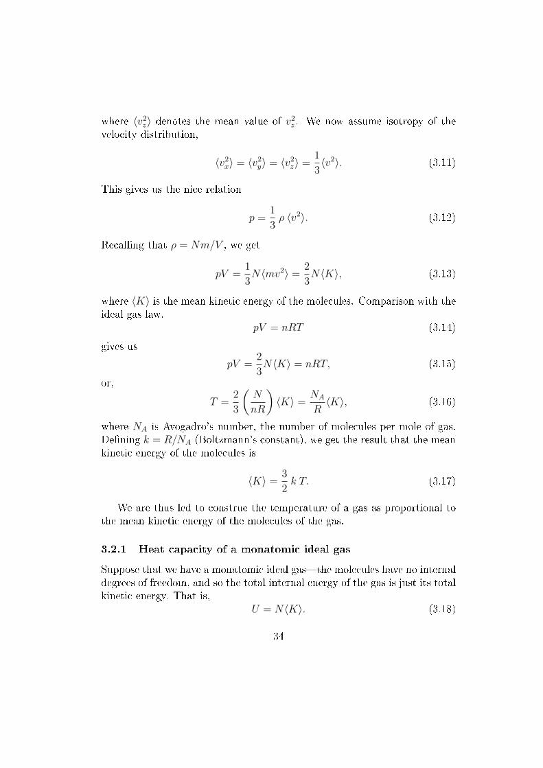
where 〈v2z〉 denotes the mean value of v2
z . We now assume isotropy of thevelocity distribution,
〈v2x〉 = 〈v2
y〉 = 〈v2z〉 =
1
3〈v2〉. (3.11)
This gives us the nice relation
p =1
3ρ 〈v2〉. (3.12)
Recalling that ρ = Nm/V , we get
pV =1
3N〈mv2〉 =
2
3N〈K〉, (3.13)
where 〈K〉 is the mean kinetic energy of the molecules. Comparison with theideal gas law,
pV = nRT (3.14)
gives us
pV =2
3N〈K〉 = nRT, (3.15)
or,
T =2
3
(N
nR
)〈K〉 =
NA
R〈K〉, (3.16)
where NA is Avogadro's number, the number of molecules per mole of gas.Dening k = R/NA (Boltzmann's constant), we get the result that the meankinetic energy of the molecules is
〈K〉 =3
2k T. (3.17)
We are thus led to construe the temperature of a gas as proportional tothe mean kinetic energy of the molecules of the gas.
3.2.1 Heat capacity of a monatomic ideal gas
Suppose that we have a monatomic ideal gasthe molecules have no internaldegrees of freedom, and so the total internal energy of the gas is just its totalkinetic energy. That is,
U = N〈K〉. (3.18)
34

Comparison with (3.17) gives
U =3
2nRT = ncvT, (3.19)
which gives the result that the molar specic heat of a monatomic ideal gasis
cV =3
2R. (3.20)
This gives, in turn,
cp = cV +R =5
2R, (3.21)
and
γ =cpcV
=5
3. (3.22)
35

4 The Second Law Revised
4.1 Tensions between thermodynamics and kinetic the-
ory
In the previous section, we saw some promising rst steps towards the re-duction of the thermodynamics of gases to kinetic theory. However, here aresome tensions between the kinetic theory of gases and thermodynamics aswe have been conceiving it.
• We have been treating of equilibrium as a state in which nothing hap-pens (cf. quote from Atkins at beginning of 2.-1). On the kinetictheory, an equilibrium state is a state that is seething with activity.
• We have been treating a gas in equilibrium as if it is a uniform sub-stance, with uniform temperature and pressure throughout. On a mi-croscopic level, however, it is far from uniform! The pressure exertedon the sides of its container is neither steady nor uniform thoughit will average out to something approximately steady and uniform, aslong as we consider areas large enough and times long enough that alarge number of molecular collisions are involved.
• We have taken the distinction between energy transfer as work, andenergy transfer as heat, to be a clear one. On the kinetic theory, how-ever, to heat something is to convey kinetic energy to its molecules.The dierence becomes: when I do work on a system, say, by mov-ing a piston, the parts of the piston move in an orderly fashion, all inthe same direction, whereas, when I heat something, the added motionof the molecules is scattered in a higgedly-piggledy fashion. Is this adistinction that holds up at the molecular level?
• Thermodynamics distinguishes between reversible and irreversible pro-cesses. The molecular dynamics are TRI (unless those need revision,too).
The last is the most serious, and is what convinced people that thermody-namics, as conceived, wasn't quite right, and what was to be reduced was arevised version.
36

4.2 The Reversibility Argument
In the decade 1867-1877, the major gures working on the kinetic theorycame to realize that the 2nd law of thermodynamics, as it had been conceived,was not to be recovered from the kinetic theory. At best one could recovera weaker version that could nonetheless account for the empirical evidencein favour of the 2nd law as originally conceived. Moreover, it seemed thatsome notion of probability was required; what the original version deemedimpossible was to be regarded as merely highly improbable.
It was considerations of reversibility of molecular dynamics that led tothese conclusions. If the molecular dynamics are TRI, then the temporalinverse of any dynamically possible process is also dynamically possible, in-cluding those that are regarded as thermodynamically irreversible.
On a letter fromMaxwell dated Dec. 11, 1867 (the letter in which Maxwellintroduced Tait to the creature came to be called Maxwell's demon10),P. G. Tait wrote, Very good. Another way is to reverse the motion ofevery particle of the Universe and to preside over the unstable motion thusproduced (Knott, 1911, p. 214).
The reversibility argument is spelled out in a letter, dated Dec. 6, 1870,from Maxwell to John William Strutt, Baron Rayleigh; Maxwell follows thiswith an exposition of the demon, and then draws the
Moral. The 2nd law of thermodynamics has the same degree oftruth as the statement that if you throw a tumblerful of waterinto the sea, you cannot get the same tumblerful of water outagain (Garber et al., 1995, p. 205).
Maxwell's view is that processes that, from the point of view of thermody-namics, are regarded as irreversible, are ones whose temporal inverses are notimpossible, but merely improbable. In a letter to the editor of the SaturdayReview, dated April 13, 1868, Maxwell draws an analogy between mixing ofgases and balls shaken in a box.
10Thomson attributes the name to Maxwell:
The denition of a demon, according to the use of this word by Maxwell,is an intelligent being endowed with free will, and ne enough tactile andperceptive organisation to give him the faculty of observing and inuencingindividual molecules of matter (Thomson, 1874, p. 441).
But Maxwell says that it was Thomson who gave the creatures this name (Knott, 1911,p. 214).
37

As a simple instance of an irreversible operation which (I think)depends on the same principle, suppose so many black balls putat the bottom of a box and so many white above them. Thenlet them be jumbled together. If there is no physical dierencebetween the white and black calls, it is exceedingly improbablethat any amount of shaking will bring all the black balls to thebottom and all the white to the top again, so that the operationof mixing is irreversible unless either the black balls are heavierthan the white or a person who knows white from black picksthem and sorts them.
Thus if you put a drop of water into a vessel of water no chemistcan take out that identical drop again, though he could take outa drop of any other liquid (in Garber et al. 1995, 192193).
We nd similar considerations in Gibbs several years later,
when such gases have been mixed, there is no more impossibil-ity of the separation of the two kinds of molecules in virtue oftheir ordinary motions in the gaseous mass without any externalinuence, than there is of the separation of a homogeneous gasinto the same two parts into which it as once been divided, afterthese have once been mixed. In other words, the impossibilityof an uncompensated decrease of entropy seems to be reduced toimprobability (Gibbs 1875, 229; 1961, 167).
It was Loschmidt who, in 1876, drew Boltzmann's attention to reversibil-ity considerations. In his response to Loschmidt, Boltzmann (1877) acknowl-edged that there could be no purely dynamical proof of the increase of en-tropy.11
It is one thing to acknowledge that violations of the second law will some-times occur, albeit with low probability. Maxwell went further, assertingthat, on the small scale, minute violations of the second law will continuallyoccur; it is only large-scale, observable violations that are improbable.
the second law of thermodynamics is continually being violated,and that to a considerable extent, in any suciently small groupof molecules belonging to a real body. As the number of molecules
11For further discussion of the probabilistic turn in Boltzmann's thinking, see Unk(2007b), Brown et al. (2009).
38

in the group is increased, the deviations from the mean of thewhole become smaller and less frequent; and when the number isincreased till the group includes a sensible portion of the body, theprobability of a measurable variation from the mean occurring ina nite number of years becomes so small that it may be regardedas practically an impossibility.
This calculation belongs of course to molecular theory and notto pure thermodynamics, but it shows that we have reason forbelieving the truth of the second law to be of the nature of astrong probability, which, though it falls short of certainty byless than any assignable quantity, is not an absolute certainty(Maxwell 1878b, p. 280; Niven 1965, pp. 67071).
What is accepted by most physicists today, and goes by the name of the2nd law of thermodynamics, is something along the lines of
Although uctuations will occasionally result in heat passing spon-taneously from a colder body to a warmer body, these uctuationsare inherently unpredictable and it is impossible for there to be aprocess that consistently and reliably harnesses these uctuationsto do work.
Call this the probabilistic version of the second law of thermodynamics.
4.3 The Maxwellian View
4.3.1 A Third Second Law
Maxwell placed a further limitation on the 2nd law. For Maxwell, even theprobabilistic version of the 2nd law holds only so long as we are in a situationin which molecules are dealt with only en masse. This is the limitation ofwhich he speaks, in the section of Theory of Heat that introduces the demonto the world.
One of the best established facts in thermodynamics is that itis impossible in a system enclosed in an envelope which permitsneither change of volume nor passage of heat, and in which boththe temperature and the pressure are everywhere the same, toproduce any inequality of temperature or pressure without the
39

expenditure of work. This is the second law of thermodynamics,and it is undoubtedly true as long as we can deal with bodies onlyin mass, and have no power of perceiving the separate moleculesof which they are made up. But if we conceive of a being whosefaculties are so sharpened that he can follow every molecule inits course, such a being, whose attributes are still as essentiallyas nite as our own, would be able to do what is at presentimpossible to us. For we have seen that the molecules in a vesselfull of air at uniform temperature are moving with velocities byno means uniform, though the mean velocity of any great numberof them, arbitrarily selected, is almost exactly uniform. Now letus suppose that such a vessel is divided into two portions, a andb, by a division in which there is a small hole, and that a being,who can see the individual molecules, opens and closes this hole,so as to allow only the swifter molecules to pass from a to b, andonly the slower ones to pass from b to a. He will thus, withoutexpenditure of work, raise the temperature of b and lower thatof a, in contradiction to the second law of thermodynamics.
This is only one of the instances in which conclusions which wehave drawn from our experience of bodies consisting of an im-mense number of molecules may be found not to be applicableto the more delicate observations and experiments which we maysuppose made by one who can perceive and handle the individualmolecules which we deal with only in large masses. (Maxwell,1871, pp. 308309).
Note that there is in this no hint that there might be some principle of physicsthat precludes the manipulations of the demon, or constrains it to dissipatesucient energy that the net change of entropy it produces is positive. More-over, Maxwell leaves it open that the requisite manipulations might becometechnologically possible in the futurethe demon does what is at present
impossible for us. What Maxwell is proposing, as a successor to the secondlaw, is strictly weaker than the probabilistic version. For Maxwell, even theprobabilistic version is limited in its scopeit holds only in circumstances inwhich there is no manipulation of molecules individually or in small numbers.
40

4.3.2 Maxwell on thermodynamics
Maxwell's conception of the status of the second law ties in with his concep-tion of the status and purpose of the science of thermodynamics.
Central to thermodynamics is a distinction between two ways in whichenergy can be transferred from one system to another: it can be transferredas heat, or else one system can do work on the other. The second lawof thermodynamics requires, for its very formulation, a distinction betweenthese two modes of energy transfer. In Clausius' formulation,
Heat cannot pass from a colder body to a warmer body withoutsome other change connected with it occurring at the same time.12
To see that this hangs on a distinction between heat and work, note that itbecomes false if we don't specify that the energy is transferred as heat. Itis not true that no energy can be conveyed from a cooler body to a warmerbody without some other change connected with it: if two gases are separatedby an insulating movable piston, the gas at higher pressure can compressthat is, do work on the gas at lower pressure, whatever their respectivetemperatures.
The Kelvin formulation of the second law is,
It is impossible, by means of inanimate material agency, to derivemechanical eect from any portion of matter by cooling it belowthe temperature of the coldest of the surrounding objects (quotedin Unk 2001, p. 327).
This statement does not say that we cannot cool a body below the temper-ature of the coldest surrounding objects. Refrigerators are possible. Thedierence is: though we can derive mechanical eectthat is, do work byextracting heat from a hotter body, using some of the energy to do work, anddiscarding the rest into a cooler reservoir, extraction of heat from a body thatis already cooler than any body that might be used as a reservoir requires theopposite of deriving mechanical eect: it requires us to use up some energythat could have been used for mechanical eect, in order to eect the trans-fer. Thus the Kelvin statement, also, requires a distinction between derivingmechanical eect from a body and extracting heat from it.
12Es kann nie Wärme aus einem kälteren Körper übergehen, wenn nicht gleichzeitigeine andere damit zusammenhängende Aenderung eintritt. Quoted by Unk (2001, p.333).
41

What is this distinction? On the kinetic theory of heat, when a body isheated, the total kinetic energy of its molecules is increased, so, for body Ato heat body B, parts of A must interact with parts of B to change theirstate of motion. When A does work on B, it is again the case that parts of Aact on parts of B to change their state of motion. The dierence is: in heattransfer, energy is transferred to the parts of the body in a haphazard way;the resulting motions cannot be tracked. This limits our ability to recoverthe energy as work.
Put this way, the distinction seems to rest on anthropocentric consid-erations, or, better, on consideration of the means we have available to usfor keeping track of and manipulating molecules. We shall call considera-tions that turn on the means available to an agent for gathering informationabout a system or for manipulating it means-relative; these are matters thatcan vary between agents, but it would be misleading to call them subjec-tive, as we are considering limitations on the physical means that are at theagents' disposal. On Maxwell's view, the distinction between work and heatis means-relative.
Available energy is energy which we can direct into any desiredchannel. Dissipated energy is energy we cannot lay hold of anddirect at pleasure, such as the energy of the confused agitationof molecules which we call heat. Now, confusion, like the correl-ative term order, is not a property of material things in them-selves, but only in relation to the mind which perceives them. Amemorandum-book does not, provided it is neatly written, appearconfused to an illiterate person, or to the owner who understandsthoroughly, but to any other person able to read it appears to beinextricably confused. Similarly the notion of dissipated energycould not occur to a being who could not turn any of the energiesof nature to his own account, or to one who could trace the mo-tion of every molecule and seize it at the right moment. It is onlyto a being in the intermediate stage, who can lay hold of someforms of energy while others elude his grasp, that energy appearsto be passing inevitably from the available to the dissipated state(Maxwell 1878a, p. 221; Niven 1965, p. 646).
That there is some energy that, for us, counts as dissipated energy hasto do, according to Maxwell, with the large number and small size of themolecules that make up a macroscopic body.
42

The second law relates to that kind of communication of energywhich we call the transfer of heat as distinguished from anotherkind of communication of energy which we call work. Accord-ing to the molecular theory the only dierence between thesetwo kinds of communication of energy is that the motions anddisplacements which are concerned in the communication of heatare those of molecules, and are so numerous, so small individually,and so irregular in their distribution, that they quite escape allour methods of observation; whereas when the motions and dis-placements are those of visible bodies consisting of great numbersof molecules moving all together, the communication of energy iscalled work (Maxwell 1878b, p. 279; Niven 1965, p. 669).
If heat and work are means-relative concepts, then perforce so is entropy.The entropy dierence between two equilibrium states of a system is givenby
∆S =
∫d Q
T,
where the integral is taken over any quasistatic process joining the two states,and d Q is the increment in heat absorbed from the system's environment.Thus, on Maxwell's view, the very concepts required to state the second lawof thermodynamics are means-relative. For more on the Maxwellian view ofthermodynamics and statistical mechanics, see Myrvold (2011).
4.4 Exorcising Maxwell's Demon
If a machine is possible that could behave as a Maxwell Demon, and if thismachine could operate without a compensating increase of entropy either inits own internal state or in some auxiliary system, then even the probabilis-tic version of the Second Law is false. Most physicists believe that such amachine is, indeed, impossible. There is less consensus on why.
To operate reliably, the Demon must:
1. Make an observation regarding the position and velocity of an incomingmolecule,
2. Record the result, at least temporarily,
3. Operate the trap-door dividing the two sides of the vessel of gas,
43

4. If operating reversibly, erase the record of the observation.
If the statistical version of the Second Law is not to be violated, thenthis series of activities must, on average, generate an increase of entropy atleast as great as the entropy decrease eected in the gas. In 1929, Szilard,basing his calculation on a simple one-molecule engine, concluded,
If an information processing system gains information sucientto discriminate among n equally likely alternatives, this must onaverage be accompanied by an entropy increase of at least k log n.
This is known as Szilard's Principle. In 1961, Landauer concluded
If an information processing system erases information sucientto discriminate among n equally likely alternatives, this must onaverage be accompanied by an entropy increase of at least k log n.
This is known as Landauer's Principle.These principles are argued for on the assumption of the correctness of
the statistical version of the Second Law. They may be correct, but invokingthem would not help convince a modern Maxwell, skeptical of the SecondLaw, of its correctness. For more discussion of Maxwell Demons, see Earmanand Norton (1998, 1999); Le and Rex (2003); Norton (2005, 2011).
44

5 The Boltzmann H-theorem and its discon-
tents
A simple kinetic model of the ideal gas has led to the identication of ther-modynamic variables with aggregate properties of molecules: pressure as theaverage force per unit area exerted on the sides of the container (or objectsuspended in the gas), temperature as proportional to mean kinetic energyof the molecules. We want more: we want construal of entropy in molecularterms, and an explanation of the approach to equilibrium.
Boltzmann's H-theorem was an important step towards the latter. Boltz-mann considered how the distribution of the velocities of the molecules of agas could be expected to change under collisions, argued that there was aunique distributionnow called the Maxwell-Boltzmann distributionthatwas stable under collisions, and, moreover, that a gas that initially had adierent distribution
Maxwell-Boltzmann distribution: the fraction of molecules having veloc-ity in a small volume in v-space, [vx, vx + δvx]× [vy, vy + δvy]× [vz, vz + δvz],is proportional to
e−mv2/2kT δvxδvyδvz. (5.1)
To argue that this was the unique equilibrium, which would be approachedif we started with a dierent distribution, Boltzmann dened a quantity,(now) called H, showed that it reached a minimum value for this distribu-tion, and argued that it would decrease to its minimum.13
5.1 The Ehrenfest wind-tree model
Rather than go into the intricacies of the H-theorem, we will look at a sim-ple toy model (the `wind-tree model') due to the Ehrenfests (Ehrenfest andEhrenfest, 1990, pp. 1013) , that is easy to analyze but share some salientfeatures with Boltzmann's gases.
The model is two-dimensional. Molecules of `wind' move in a plane. Allhave same speed v, and each moves in one of four directions: north, south,east, west. Scattered randomly throughout the plane are square obstacles`trees' which don't move, with sides of length a. These have their diagonals
13Why `H'? The quantity (as we shall see) is related to the entropy, and indeed,Boltzmann originally used `E'. There is some reason to believe that H is meant to be acapital η. See Hjalmars (1977), if you care.
45

aligned with the north-south and east-west directions, so that, when a windmolecule hits one, it is deected into one of the other four directions. Thetrees have uniform mean density n per unit volume.
We want to know how a given initial distribution of wind-velocities willchange with time. Consider a small time δt. A given wind-molecule, say,one moving east, will change velocity during this time i it hits a tree, inwhich case it will be deected either to the north or to the south. For anygiven tree, the region containing wind-molecules which will be deected tothe north has area a vδt. We can therefore talk about east-north collisionareas, etc.
We assume:
The fraction of all east-travelling molecules that happen to lie ineast-north collision strips is equal to the proportion of the planeoccupied by such strips.
And, of course, we make the corresponding assumption for all the otherdirections. Call this the Stoÿzahlansatz : collision-number assumption.14
Note that we made a similar assumption regarding velocity distribution inour derivation of the pressure of an ideal gas.
The proportional area of collision-strips of each type is nav δt, where nis the number of trees per unit area. Dene α = nav. Let fi = ni/N (wherei takes as values n, s, e, w) be the fraction of all wind-molecules travellingin the i-direction. From the Stoÿzahlansatz it follows that, in a time δt, afraction 2αδt of east-moving molecules will be deected into other directions.At the same time a fraction α δt of north-moving molecules will be deectedinto the east direction, and the same fraction of south-moving molecules.This gives us
δfe = (−2αfe + αfn + αfs) δt. (5.2)
This, and corresponding considerations for the other directions, gives us thesystem of equations,
dfe/dt = −2αfe + α(fn + fs)
dfw/dt = −2αfw + α(fn + fs)
dfn/dt = −2αfn + α(fe + fw)
dfs/dt = −2αfs + α(fe + fw) (5.3)
14The translator of the Ehrenfests' book left certain key termsStoÿzahlansatz,Umkehreinwand, Wiederkehreinwanduntranslated, and the tradition among commen-tators has been to follow suit.
46

Inspection of the system of equations (5.3) shows that a stationary solutionis obtained when all the fi's are equal; that is,
fe = fn = fw = fs =1
4. (5.4)
It's not hard to get an explicit solution for our system of equations, givenarbitrary initial frequencies (details in 5.1.2, below). The upshot is: what-ever the initial frequencies are, we get an exponential approach to the equi-librium state.
5.1.1 The wind-tree H-theorem
DeneH = N
∑i
fi log fi, (5.5)
where the sum is taken over the directions for which fi 6= 0.15
Because, for all i, 0 ≤ fi ≤ 1, H cannot be positive. It takes its maximumvalue of 0 when all the molecules are going the same direction; that is, oneof the fi's is 1, and all the others 0. It takes its minimum value in theequilibrium state, when all the fi's are the same. H is, therefore, in somesense an estimate of how close the gas is to equilibrium.
Consider the rate of change of this quantity,
dH/dt = N∑i
(dfi/dt) log fi +N∑i
dfi/dt
= N∑i
(dfi/dt) log fi. (5.6)
A bit of algebra gives us
dH/dt = −Nα[(fe − fn) log
(fefn
)+ (fe − fs) log
(fefs
)+ (fw − fn) log
(fwfn
)+ (fw − fs) log
(fwfs
)](5.7)
The quantity in square brackets in (5.7) is non-negative, because, for anypositive x, y,
(x− y) log
(x
y
)≥ 0. (5.8)
15If you like, you can think of this as adopting the convention: 0× log 0 = 0.
47

Thus, we can conclude, that, in any state,
dH
dt≤ 0, (5.9)
Moreover, dH/dt = 0 only in the equilibrium state fi = const. This givesus a simple way to conclude that, for arbitrary initial frequencies, the stateapproaches the equilibrium state, where it takes its minimum value.
This is a temporally asymmetric conclusion. The evolution of the fre-quencies expressed by equations (5.3) is not invariant under time-reversal.But the underlying dynamics of collisions is TRI. This means that we musthave used an assumption to get from the dynamics to the equations (5.3) thatintroduces a temporal asymmetry. But the only assumption we used was theStoÿzahlansatz . And, indeed, it is a temporally asymmetric assumption (ifwe're not in the equilibrium state).
This is easiest to see if we consider the extreme disequilibrium state.Suppose that, at t = 0, fe = 1, and that the Stoÿzahlansatz holds. A timeδt later, a fraction 2αδt of the molecules have been scattered, half into thenorth-direction, half into the south. Suppose, now, we reverse the velocities,and ask what fraction of, say, the north-travelling molecules will collide witha tree in time δt. Answer: all of them! The wind-molecules that are nottravelling in the west direction are all on collision courses that will turnthem into west-travelling molecules.
We may nd the Stoÿzahlansatz to be a reasonable assumption in theforward direction, but its temporal reverse is certainly not, unless the stateis already an equilibrium state. The intuition here seems to have somethingto do with causality. We might expect the velocity of a molecule to beindependent of what interactions lie to its near future. We don't expect itsvelocity to be independent of interactions in its recent past. This suggests anattitude towards the temporal asymmetry of thermodynamics that groundsthermodynamic asymmetry on the temporal asymmetry of causality. Thisseems a promising avenue, though it is not one that has been popular; see,however, Oliver Penrose (2001).16
16Don't confuse Oliver Penrose, who specializes in statistical mechanics, with his brotherRoger, who also has views on temporal asymmetry!
48

5.1.2 Explicit solution for wind-tree model
It's handy to write the system of equations (5.3) in matrix form. Writingf = (fe, fw, fn, fs), let us rewrite our equations as,
df/dt = Cf . (5.10)
where
C =
−2α 0 α α
0 −2α α αα α −2α 0α α 0 −2α
(5.11)
The solution is give byf(t) = U(t) f0, (5.12)
Comparison of (5.10) and (5.12) tells us that
dU/dt = CU. (5.13)
You can easily verify that this is solved by
U(t) =1
4
1 1 1 11 1 1 11 1 1 11 1 1 1
+1
4
1 1 −1 −11 1 −1 −1−1 −1 1 1−1 −1 1 1
e−4αt+1
2
1 −1 0 0−1 1 0 0
0 0 1 −10 0 −1 1
e−2αt
(5.14)As t increases, this decays exponentially to
U∞ =1
4
1 1 1 11 1 1 11 1 1 11 1 1 1
, (5.15)
which takes arbitrary initial frequencies into the equilibrium state.
5.2 Boltzmann's H-theorem
In his original presentation (1872) of the H-theorem, Boltzmann gave theimpression that the approach to equilibrium was a consequence of the lawsof mechanics alone, applied to molecular collisions. This can't be right! Twotypes of objection showed that it can't be right:
49

• The reversibility objection (Umkehreinwand).17 For any set of tra-jectories of the molecules of a gas, the time-reversed trajectories arealso possible. Hence, a monotonic decrease of anything can't be a con-sequence of the microphysical dynamics alone.
• The recurrence objection (Wiederkehreinwand). (Raised by Zer-melo.) Take a classical system, conned to a bounded phase space (e.g.a gas in a box, with xed total energy). Consider a small open neigh-bourhood of the initial state, and ask, will the state of the system, afterit leaves that neighbourhood, ever return to it? Poincaré's recurrencetheorem answers: yes, for almost all initial phase space-points, where`almost all' means `all except for a set of Lebesgue measure zero.18
This has the paradoxical-sounding consequence that a gas that startsout in a non-equilibrium state, though it may relax to equilibrium ina short time, will, if left to itself long enough, almost certainly returnarbitrarily close to its initial state.
Can this possibly true? Would a box of gas, left on its own, eventually sponta-
neously end up occupying only half of the box? Lest this sound like mathemat-ics gone mad, recall that we have already acknowledged, as an unsurprisingconsequence of the kinetic theory, the existence of small pressure uctua-tions. The Poincaré recurrence theorem says that, if you wait long enough,all sorts of pressure uctuations occur in an isolated gas combined to a box.In his book on non-eq SM, Dorfman provides some illuminating calculationsof Poincaré recurrence times. Following is a table of the time you would haveto wait before you would expect to see a 1% uctuation of the pressure in asphere of radius a of a gas at standard temperature and pressure(Dorfman,1999).
a (cm.) tr (sec.)10−5 10−11
2.5× 10⁻⁵ 13× 10−5 106
5× 10⁻⁵ 1068
1 101014
17Credited by the Ehrenfests to Loschmidt, though there had been some discussion ofthis among the English physicists.
18If the phrase `Lebesgue measure' is unfamiliar, your intuitive idea of phase spacevolume will suce.
50

The reversibility objection applies to our wind-tree model. The recurrenceobjection does not, in the original formulation, which has the wind-tree forestspread out over an innite plane. It would apply if we put it in a nite box.
What do these two objections show? First of all, they emphasize thatthe monotonic decrease of H to its equilibrium value is not a consequence ofthe molecular dynamics alone. Something else is needed: the Stoÿzahlansatz.Moreover, they tell us something about this assumption. Away from equi-librium, it cannot hold in both temporal directions. And, even it holds atsome initial time, it cannot remain true indenitely, for a bounded, isolatedsystem.
Intuitively: even if the Stoÿzahlansatz is valid at some particular time t0,
• Though the state of a molecule at t0 is independent of what lies aheadof it in its near future (and will continue to be at least approximatelyso, for some time), its state shortly after t0 will not be independent ofinteractions in its recent past.
• Over long enough time periods, as molecules encounter molecules withwhich they have interacted, the correlations built up via past interac-tions become relevant, and so the Stoÿzahlansatz cannot be regardedas a reasonable approximation arbitrarily far into the future.
5.3 The signicance of H
5.3.1 Wind-tree H
The detailed microscopic state of the wind-tree gas requires specication ofposition and velocity of each of the individual molecules. We have repre-sented the macro-state by specication of the numbers ne, nw, nn, ns ofmolecules with each v-direction. If there are N wind-molecules in total, fora given macrostate ne, nw, nn, ns the number of distinct distributions ofwind-molecules among the four directions that agree with this macrostate is
Ω =N !
ne! nw! nn! ns!. (5.16)
This giveslog Ω = logN !−
∑i
log ni! (5.17)
51

To get a handle on this, apply Stirling's approximation formula,
logN ! ≈ N logN −N. (5.18)
This gives us (remembering that∑
i ni = N),
log Ω ≈ N logN −∑i
ni log ni
= N
(logN −
∑i
fi log(Nfi)
)= −N
∑i
fi log fi = −H, (5.19)
or,H ≈ − log Ω. (5.20)
5.3.2 Boltzmann's H and Boltzmann's entropy
Consider a gas made up of N molecules, each having r degrees of freedom.The phase space of each molecule, called µ-space, is 2r-dimensional. Thephase space of the gas, called Γ-space, is 2Nr-dimensional.
Let us partition µ-space into compartments ωi, of equal volume [ω].For any state of the gas (that is, any point x ∈ Γ) let ni be the numberof molecules that, when the gas is in state x, occupy ωi. Consider the set(called a `Z-star') of points in Γ that have the same occupation-numbers asx. The number of distinct ways to achieve a given n = ni will be
Ω =N !
n1! n2! ...nk!, (5.21)
where, of course, we only have to include occupation-numbers ni thathappen to be nonzero. Therefore, the volume of the region of Γ-space sharingx's set of occupation numbers is
Ω [ω]N =N !
n1! n2! ...nk![ω]N . (5.22)
As before, we will have (for N suciently large for application of Stirling'sapproximation),
log Ω ≈ −N∑i
fi log fi, (5.23)
52
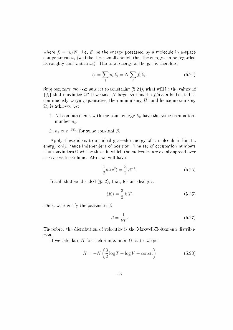
where fi = ni/N . Let Ei be the energy possessed by a molecule in µ-spacecompartment ωi (we take these small enough that the energy can be regardedas roughly constant in ωi). The total energy of the gas is therefore,
U =∑i
ni Ei = N∑i
fi Ei. (5.24)
Suppose, now, we ask: subject to constraint (5.24), what will be the values offi that maximize Ω? If we take N large, so that the fi's can be treated ascontinuously varying quantities, then minimizing H (and hence maximizingΩ) is achieved by:
1. All compartments with the same energy Ek have the same occupation-number nk.
2. nk ∝ e−βEk , for some constant β.
Apply these ideas to an ideal gasthe energy of a molecule is kineticenergy only, hence independent of position. The set of occupation numbersthat maximizes Ω will be those in which the molecules are evenly spread overthe accessible volume. Also, we will have
1
2m〈v2〉 =
3
2β−1, (5.25)
Recall that we decided (3.2), that, for an ideal gas,
〈K〉 =3
2k T. (5.26)
Thus, we identify the parameter β:
β =1
kT. (5.27)
Therefore. the distribution of velocities is the Maxwell-Boltzmann distribu-tion.
If we calculate H for such a maximum-Ω state, we get
H = −N(
3
2log T + log V + const.
)(5.28)
53

Compare this with the entropy of a monatomic ideal gas,
S = CV log T + nR log V + const.
= kN
(3
2log T + log V + const.
). (5.29)
So, we have, for a monatomic ideal gas,
S = −kH + const. (5.30)
Dene the Boltzmann entropy
SB = k log Ω. (5.31)
This has the properties:
• For an isolated gas (xed total energy), if we ask for the distributionof molecular positions and velocities that maximizes Ωthat is, theone that takes up the largest volume of Γ-spaceit's the one in whichmolecular positions are distributed evenly over the box, and velocitiesaccording to the Maxwell-Boltzmann distribution.
• In such a state, the functional dependance of SB on temperature andvolume is the same as that of the thermodynamic entropy S.
Without going into details of molecular interactions, it's at least plausiblethat molecular collisions will lead the system into `typical' regions of its phasespacethose that maximize SB. There's a temptation to put aside moleculardynamics and argue on the basis solely of phase-space volume that systemswill tend to wander into regions of higher Boltzmann entropy. But this can'tbe right. What we can hope for, however, is that such a conclusion will notdepend too sensitively on the details of the molecular dynamics. More onthis later.
5.3.3 Boltzmann entropy of an ideal gas
I exhibited the result (5.28) without the additive constants, because I wantedto emphasize the dependence on volume and temperature, and compare itwith the thermodynamic entropy, which is dened only up to an additiveconstant. Given a choice of the size of the elements partition of phase space,
54

[ω], the formula (5.31) uniquely determines the additive constant. Let's dothe detailed calculation.
Because it's easier (in this case, at least, because we know how to doGaussian integrals) to do integrals than sums, we will approximate the dis-tribution f = (fi) by a continuous function f on µ-space that varies littlewithin each partition-element ωi.
fi ≈ f(xi,pi) [ω] (5.32)
where (xi,pi) is a representative point in ωi (since f varies little in thisregion, it won't matter much which points we take). Then
H = N∑i
fi log fi = N∑i
[f(xi,pi) log f(xi,pi)] [ω] +N log[ω]. (5.33)
Since we're interested in the values of fi that maximize Ω, and the energyassociated with point (x,p) in µ-space is p2/2m, take
f(x,p) = C−1e−βp2/2m, (5.34)
where C is a normalization constant. The requirement that the integral of fover the spatial volume V , and all possible momenta, be equal to unity gives
C =
(2πm
β
) 32
V. (5.35)
We replace the sum in (5.33) with an integral,∑i
[f(xi,pi) log f(xi,pi)] [ω] ≈∫ ∫
f(x,p) log f(x,p) d3x d3p = 〈log f〉,
(5.36)where 〈 〉 denotes expectation value with respect to the measure f . We have,
〈log f〉 = − logC − β
2m〈p2〉. (5.37)
For this distribution,
〈p2〉 =3m
β, (5.38)
or,
〈K〉 =〈p2〉2m
=3
2β−1, (5.39)
55

on which we based our conclusion that β = 1/kT . So, we have
〈log f〉 = −(
logC +3
2
), (5.40)
H = −N(
logC +3
2− log[ω]
)= −N
[log
(V (mkT )3/2
[ω]
)+
3
2log 2π +
3
2
], (5.41)
or
SB = k log Ω ≈ −kH
= kN
[log
(V (mkT )3/2
[ω]
)+
3
2log 2π +
3
2
]. (5.42)
5.3.4 Gibbs' paradox
The expression (5.42) for the Boltzmann entropy of a classical, monatomicideal gas is what is yielded by a straightforward calculation. But there'ssomething wrong with itit's not an extensive quantity.
To see this, suppose that we have two samples of the same ideal gas atthe same temperature and pressure, with N1 and N2 molecules, respectively,occupying volumes V1 and V2. The combined system has N = N1 + N2
molecules and occupies a volume V = V1 + V2. Applying (5.42) to thesegases, we nd,
S 6= S1 + S2. (5.43)
In fact, we get (after a bit of algebra),
S − (S1 + S2) = kN1 log (V/V1) + kN2 log (V/V2) . (5.44)
So, if we initially have N1 molecules of a gas, occupying V1, and N2 molecules,occupying V2, and remove the partition between them, allowing them to mix,then applying (5.42) to calculate the entropy of the mixture, yields the resultthat this entropy exceeds the sum of the initial entropies by an amount equalto the entropy of mixing of two distinct gases (recall discussion in 2.4.1).This resultthat a straightforward classical calculation results in an entropyof mixing, even for samples of the same gasis called Gibbs' paradox.
56

The expression for the entropy of an ideal gas that one nds in textbooksis usually derived from a treatment of the gas as a set of quantum particlesconned to a box. This results in the Sackur-Tetrode formula,
SST = kN
[log
(V (mkT )3/2
Nh3
)+
3
2log 2π +
5
2
]. (5.45)
The N in the denominator renders it extensive: if I have samples of gas atthe same temperature and pressure, so that Vi/Ni is the same for all i, then
SST (N, V, T ) =∑i
SST (Ni, Vi, T ). (5.46)
If we compare (5.45) and (5.42), and choose, in (5.42), [ω] = h3 as the sizeof the cells of our µ-space partition, we nd that they dier by
SST − SB = −k(N logN −N) ≈ −k logN ! (5.47)
where we have once again used Stirling's approximation. The properly ex-tensive quantity SST is obtained by subtracting k logN ! from SB as obtainedby a straightforward classical calculation, or, equivalently,
SST = k log
(Ω
N !
), (5.48)
corresponding to a volume of a reduced Γ-space in which states that dif-fer only by permutations of the molecules are identied. Textbooks, (e.g.Huang (1986, 6.6)) often say that the justication of this must be quantum-mechanical, though others, (e.g. Allis and Herlin (1952); Dugdale (1996))do a classical calculation with indistiguishability built in from the start. Fordiscussion, see Saunders (2006).
57

6 Probability
6.1 Enter Probability
A system that, if out of equilibrium, approaches equilibrium, and, if in equi-librium, stays there, will be said to be exhibiting thermodynamic behavior.A system moving away from equilibrium will be said be exhibiting anti-
thermodynamic behaviour.The Reversibility and Recurrence objections to the H-theorem show ,
respectively,
• We won't see thermodynamic behaviour for all initial states of a gas.In fact, there is a one-one mapping (velocity reversal) between non-equilibrium states that move toward equilibrium, and ones that moveaway.
• A gas in a box, if isolated for a long period of time, will eventuallyexhibit anti-thermodynamic behaviour.
These facts, together with our earlier conclusion (4.2) that it is therevised, probabilistic version of the Second Law that is worth recovering,strongly suggest a revised, probabilistic version of the H-theorem, along thelines that, for macroscopic systems (i.e large numbers of degrees of free-dom), H will probably decrease to a minimum, and stay there for any timeperiod that we are likely to be observing the system (recall that Poincarérecurrence times for large uctuations are mind-numbingly long). That theH-theorem be given a statistical interpretation was suggested by the Ehren-fests (Ehrenfest and Ehrenfest, 1990). And the conclusion, in the previoussection, that states corresponding to macroscopic equilibrium occupy the pre-ponderance (with respect to a measure on phase-space that is uniform overthe energy-surface) of phase space, is certainly suggestive of a probabilisticinterpretation. But some work must be done to go from greater phase-spacevolume to more probable. Among other things, we will have to ask whatwe will mean by more probable.
58

6.2 Probability: chance and credence
6.2.1 Axioms of probability
A probability function Pr(·) maps propositions to real numbers. The domainof our probability function is assumed to be closed under Boolean combina-tions. These functions are held to satisfy the following axioms, adapted fromKolmogorov.
1. For all p, Pr(p) ≥ 0.
2. If p is logically true, Pr(p) = 1.
3. If p and q are logically incompatible, then Pr(p ∨ q) = Pr(p) + Pr(q).
There is another axiom, adopted by some and omitted by others. We rstneed an extra assumption about our set of propositions, which is that, for anysequence pi of mutually incompatible propositions, there is a proposition,which we will denote
∨i pi, that is true i one of pi is true. The fourth
axiom is called countable additivity.
4. For any sequence pi of mutually incompatible propositions,
Pr(∨i
pi) =∑i
Pr(pi).
6.2.2 Conditional probability
Given p, q, with Pr(q) 6= 0, we dene the conditional probability
Pr(p|q) =df.Pr(p&q)
Pr(q). (6.1)
Note that this has the consequence that
Pr(p&q) = Pr(p|q)Pr(q) = Pr(q|p)Pr(p), (6.2)
which entails that
Pr(p|q) =Pr(q|p) Pr(p)
Pr(q). (6.3)
This is known as Bayes' theorem.
59

6.2.3 Distinct senses of probability
As Hacking (1975) and others have pointed out, the word probability is usedto cover (at least) two distinct concepts. One concept, the epistemic concept,has to do with degrees of belief of a rational agent. The other concept, whichmay appropriately be called the aleatory concept, is the concept appropriateto games of chance; this is the sense in which one speaks, for example, of theprobability (whether known or not) of rolling at least one pair of sixes, in24 throws of a pair of fair dice. I will use the word credence for the former,epistemic concept, and chance for the aleatory concept. Chances are to bethought of as objective features of a chance set-up, such as a coin toss. Theyare, therefore, the sorts of things one can have degrees of belief about; wehave credences about the values of chances.
It can be argued (see, e.g., Greaves and Wallace (2006)) that a rationalagent, upon learning a new item of evidence e, will update her credences byconditonalizing on e. So, for any hypothesis h,
Cr(h)→ Cr(h|e) =Cr(e|h) Cr(h)
Cr(e). (6.4)
6.2.4 Evidence about chances
Suppose that you are about to toss a coin. You initially have degrees of beliefabout the value of the chance of heads on each toss. Let's pretend that thereis a discrete set λi of candidate values for the chance (this is for simplicityof exposition only; it's easy enough to lift this restriction). Let hi be thehypothesis that the chance of heads on each toss is λi.
Toss the coin 10 times, and get some result, e.g.
THHHTTHHHT
Let e be this result. The chance of this happening, if hi is true, is
ch(e|hi) = λ6i (1− λi)4. (6.5)
We want to update our credences in the hypotheses hi by conditionalizingon e
Cr(hi)→ Cr(hi|e) =Cr(e|hi) Cr(hi)
Cr(e)=
Cr(e|hi) Cr(hi)∑j Cr(e|hj)Cr(hj)
. (6.6)
We introduce a condition on rational credence, called by David Lewis (1980)the Principal Principle, that constrains the values of Cr(e|hi).
60

PP. If h entails that the chance of e is some number x, and bcontains only `admissible' information,19 then
Cr(e|h&b) = x = ch(e|h). (6.7)
The PP is a requirement that our agent's degree of belief in e meshesappropriately with her degrees of belief about the candidates for the chanceof e.
Cr(e|b) =∑i
ch(e|hi) Cr(hi|b). (6.8)
If the agent's credence satisfy the Principal Principle,
Cr(hi|e) =ch(e|hi) Cr(hi)
Cr(e). (6.9)
or,Cr(hi|e)/Cr(hi)Cr(hj|e)/Cr(hj)
=ch(e|hi)ch(e|hj)
. (6.10)
The evidence e favours hypotheses that endow e with high chance. For anysequence s of N coin tosses having n heads and m = N − n tails,
ch(s|hi) = λni (1− λi)m. (6.11)
It is easy to check that this function achieves a maximum when λi is equal tothe observed relative frequency of heads, n/N , and is more sharply peaked,the larger N is. This means that, for large N , the chance is high that therelative frequency n/N will be close to λ. In fact, it can be proven (this isBernoulli's theorem) that, for an innite sequence of ips, the chance thatthe relative frequency converges to λ is equal to 1.
A long run of repeated coin ips will strongly favour hypotheses that posita chance of heads on each ip that is close to the observed relative frequency.Credence, chance, and frequency are linked in an evidential relationship:relative frequency data from repeated experiments is evidence relevant toour credences about single-case chances.
19Lewis: Admissible propositions are the sort of information whose impact on credenceabout outcomes comes entirely by way of credence about the chances of those outcomes.In particular, e itself is not admissible.
61

6.3 Frequentism
Consider:
• If an urn contains N balls, of which m are black, and a ball is drawnin such a way that each ball has an equal chance of being the onedrawn, then the chance that the ball drawn is black is equal to m/N ,the relative frequency of black balls in the urn.
• In an innite series of Bernoulli trials (this means: successive trialsindependent, with chance of each possible outcome same on each trial),the chance is equal to one that the relative frequency of outcome x willconverge as n→∞ (and, moreover, will converge to the chance of x ineach individual trial).
• Relative frequency data can provide evidence about values of chances.
There are, therefore, intimate connections between chances and relativefrequencies. This (together, I think, with worries about what objectivechance could mean in a deterministic world), has suggested to some that theprobability, in the objective sense, be identied with relative frequenciesin either actual or hypothetical sequences of events. This became a popularidea in the 19th century. John Venn's book The Logic of Chance (1866) isone source of this view. An inuential 20th-century proponent of the viewwas Ludwig von Mises, who defended a view of probabilities as frequenciesin hypothetical innite sequences he called Kollektivs.
Most (but not all) philosophers these days think that a frequency interpre-tation of probability is untenable. The intuition underlying von Mises, thatfrequencies would converge if certain trials were continued indenitely, seemsto be based on the Bernoulli theorem and related convergence theorems,whose very statement requires a notion of chance independent of frequency:they say that, with chance equal to one, relative frequencies will converge.Similarly, the conclusion that the probability that a ball drawn from an urnbe black is equal to the relative frequency of black balls in the urn requiressome notion that each ball have an equal chance of being drawn. And thereis the problem of the reference class : if I want to identify an objective prob-ability that a certain item have property P with the relative frequency of Pin some class of similar items, this will vary depending on the choice of theclass to which the probability is referred. Furthermore, if all I know is thatthe nite sequence of coin tosses I'm about to see is an initial segment of an
62
innite sequence in which the relative frequency of H converges to 1/2; thistells me nothing at all about the nite initial sequence. Why? Because, if Itake an innite sequence in which the frequency of heads converges to 1/2,and tack on any arbitrary initial nite sequence, no matter how long, thenthe new sequence has exactly the same convergence properties as the old.
6.4 Classical Probability and Symmetries
Classical probability theory is mostly concerned with situations, approxi-mated by gambling set-ups, in which there is a partition of possible out-comes into equally probable classes (think dice tosses, coin tosses, roulettewheels). Laplace used this as the basis for probability theory, in his seminalPhilosophical Essay on Probability (1814). Therein he wrote,
The curve described by a simple molecule of air or vapor is regu-lated in a manner just as certain as the planetary orbits; the onlydierence between them is that which comes from our ignorance.
Probability is relative, in part to this ignorance, in part to ourknowledge. We know that of three or a greater number of eventsa single one ought to occur; but nothing induces us to believethat one of them will occur rather than the others. In this stateof indecision it is impossible for us to announce their occurrencewith certainty. It is, however, probable that one of these events,chosen at will, will not occur because we see several cases equallypossible which exclude its occurrence, while only a single onefavors it.
The theory of chance consists in reducing all the events of thesame kind to a certain number of cases equally possible, that isto say, to such as we may be equally undecided about in regard totheir existence, and in determining the number of cases favorableto the event whose probability is sought. The ratio of this numberto that of all the cases possible is the measure of this probability,which is this simple a fraction whose numerator is the number offavorable cases and whose denominator is the number of all thecases possible.
63

Note that there is a qualication: we must judge the cases to be equallypossible, which seems to be synonymous with equally probable20 If this iswhat it means, then we can't take this, on pain of circularity, as a denitionof probability. What Laplace can be thought of as doing is: showing us how,given judgments of equiprobability, to get other probabilities out of thesejudgments.
There is a temptation to think that a judgment of which events areequally probable is dispensable, and that we can dene probability as ra-tio of favourable cases to total number of cases. In fact, Laplace rst doesthis, when he is laying down principles, then corrects himself:
First Principle.The rst of these principles is the denitionitself of probability, which, as has been seen, is the ratio of thenumber of favorable cases to that of all the cases possible.
Second Principle.But that supposes the various cases equallypossible. If they are not so, we will determine rst their respectiveprobabilities, whose exact appreciation is one of the most delicatepoints of the theory of chance.
Yes, indeed! There has been extracted from Laplace a Principle of Indif-ference, which says
If you have no information about a set of mutually exclusive pos-sibilities, assign them equal probabilities.
This can lead to absurd results if applied incautiously. Consider a coinabout to be tossed twice. The natural choice of equiprobable partition isHH,HT, TH, TT, each of which is to be assigned equal probability 1/4.But someone might reason: there are three possibilities for the number ofheads, and each of these is equiprobable.
In this case, there is a natural-seeming choice of equipartition. Things getmore complicated, though, when there is a continuum of possibilities. Theremight not be a natural choice for a variable that is uniformly distributed.Consider, for example, a number x to be chosen from the interval [0, 1]. Thisis equivalent to a choice of x2, as, on this interval the mapping x ↔ x2 isone-one. Consider: what is the chance that x > 1/2? If this chance is 1/2,then there is chance 1/2 that x2 > 1/4; and so the chance that x2 > 1/2 isless than 1/2.
20See Hacking (1971) for discussion.
64

Say that a probability distribution is uniform in x, on the interval [0, 1],if for any subinterval ∆ ⊆ [0, 1], Pr(x ∈ ∆) is equal to the length of ∆.Then a probability distribution that is uniform in x is not uniform in x2,and vice versa. This matters for statistical mechanics, because, if we want totalk about probabilities being uniform over a system's state space, we haveto know: uniform in what variables? Any argument that an appropriateprobability distribution for systems in equilibrium is one that is uniformover energy surfaces, i.e. uniform in the phase space variables (x,p), willhave to invoke (or so it seems) some sort of physical considerations, involvingthe dynamics of the system.
If I know something about symmetries that a set of objective chancessatisfy, then this knowledge can be useful. For example, if I know thatchances are invariant under a swap H ↔ T , then I know that ch(H) =ch(T ) = 1/2. More on symmetry reasoning about chances, later. Also, see,if you're interested, Ch. 12 of (van Fraassen, 1989).
6.4.1 Knowledge from ignorance?
Laplace's use of `probability' seems to be ambiguous between chance andcredence. And this poses a danger. If we don't distinguish between chanceand credence, calling them both `probability,' there is a risk of sliding into afallacy (not, I must say, one that Laplace can be saddled with). Suppose Iknow nothing about a die, except that it looks symmetrical to me. I knowof no reason why one face will be favoured over another. I therefore, haveequal credence in each face being the one to land face up. There is a dangerof sliding from this, into a claim that I am certain that the chances areequal. And this is a very strong claim, not one derivable from ignorance! Ajudgment of equal chance is not an absence of judgment.
Something like this seems to be going on in, e.g, Jackson (1968). See pp.8-9, 83. (Quoted in Myrvold (2012b)).
65

6.5 Measure spaces and measures
A measurable space is a set X, together with a set S of subsets of X (themeasurable subsets of X), such that:
1. X ∈ S
2. For every S ∈ S, its complement X \ S is also in S.
3. If Ai : i ∈ N is a sequence of sets in S, their union,⋃iAi, is also in
S.
These conditions dene a σ-algebra. A σ-algebra that is often of partic-ular interest, when X is endowed with a natural topology, is comprised bythe Borel subsets of X: the smallest σ-algebra containing all the open sets.
Not all subsets of Rn are Borel sets, hence not all will be assigned ameasure on the measures with which we will be concerned, but this willmake little dierence.
A measure on a measurable space is a function µ : S → R+ such that:
1. µ(∅) = 0.
2. If Ai is a sequence of mutually disjoint sets in S,
µ(⋃i
Ai) =∑i
µ(Ai). (6.12)
A measure is unital i µ(X) = 1.Suppose I have a physical system whose state is represented by a point x in
a state space X. Then, for every subset S ⊆ X, there will be a correspondingproposition x ∈ S.
If 〈X,S〉 is a measurable space, then every unital measure µ denes aprobability function, dened on propositions of the form x ∈ S, where S ∈ S.
Pr(x ∈ S) = µ(S). (6.13)
66

6.6 Probability ow; Liouville's theorem
Suppose that, at some time t0, the probability (be it chance or credence)that the state of our system is in S ⊆ X is given by the measure ρ0(S). Letthe system evolve to time t1. Each point in S will evolve to a new point. LetU(S) be the set of points that S evolves into. Then, the probability that,at time t1, the system is in the set U(S), is the same as the probability thatit was in set S at time t0. We can dene a new probability measure on thephase space by
ρ1(U(S)) = ρ0(S), (6.14)
or,ρ1(S) = ρ0(U−1(S)). (6.15)
Since we can do this for any time, we can dene a family of probabilitymeasures, ρ(t), and we can picture the action of the dynamical evolution ofthe system as a probability ow.
One denes a dynamical system as a quadruple 〈X,S, µ, φt〉, where X is astate space, S a σ-algebra (the measurable subsets of X), µ a unital measureon S, and φt : X → X a semi-group of maps from X into itself, representingthe dynamical evolution of the system.
You may have encountered, in continuum mechanics, a continuity equa-tion for the ow of a uid. A uid with density ρ(x, t) and velocity-eldv(x, t) satises,
∂ρ
∂t+∇ · (ρ v) = 0. (6.16)
(This is because the rate of change of the amount of the uid in any boundedvolume must be equal to the rate of ow across the surface of the volume.Apply the Divergence Theorem.)
Our probability density ρ is dened on phase space Γ, which is parame-terized by the full set of coordinates and conjugate momenta for all degreesof freedom of the system: (qi, pi) : i = 1, ..., dim(Γ)/2. The continuityequation for our probability ow is therefore,
∂ρ
∂t+∑i
∂
∂qi(ρ qi) +
∑i
∂
∂pi(ρ pi) = 0. (6.17)
Suppose, now, that the system obeys Hamilton's equations of motion,
qi =∂H
∂pipi = −∂H
∂qi. (6.18)
67

This gives us Liouville's theorem
∂ρ
∂t+∑i
(∂ρ
∂qi
∂H
∂pi− ∂ρ
∂pi
∂H
∂qi
)= 0. (6.19)
Apply this to the measure that is uniform over phase space: ρ(q,p) =const.. Then ∂ρ/∂qi = ∂ρ/∂pi = 0, and so
∂ρ
∂t= 0. (6.20)
The uniform measure on phase space is invariant under dynamical evolution.Similarly, any measure that is uniform on energy surfaces is invariant. Sup-pose that ρ can be represented by a density function that is a function of theHamiltonian: ρ(q,p) = f(H(q,p)). Then
∂ρ
∂qi
∂H
∂pi− ∂ρ
∂pi
∂H
∂qi= f ′(H)
(∂H
∂qi
∂H
∂pi− ∂H
∂pi
∂H
∂qi
)= 0.
68

7 Probabilities in Statistical Mechanics
7.1 The brute posit.
One approach to probabilities in statistical mechanics (see e.g. Tolman(1938)) is to simply include, as a postulate of the theory, that the probabilityof a system being in a certain microstate, given macroscopic constraints, isuniform on energy surfaces consistent with the microstate. This gives rise tothe most commonly used probability distributions:
• The microcanonical distribution. Appropriate for an isolated system,which has a xed energy. Take a region of phase space containing allstates with energy in a narrow band [E,E+δE], and take a probabilitydistribution that is uniform, in canonical phase space variables, in thissmall region. One can also dene a probability distribution on thesurface of energy E by taking a limit.
• The canonical distribution. Appropriate for systems in contact with aheat bath of xed temperature (the system can exchange energy withthe heat bath, and hence its energy can vary.) Given by
ρ(q,p) ∝ e−βE(q,p), (7.21)
where E(q,p) is the energy of the system in state (q,p), and, as be-fore, β = 1/kT . Because physicists, from the time of Gibbs, havetended to visualize probability distributions as large collections of sys-tems subjected to the same preparation procedure, the terminologymicrocanonical ensemble and canonical ensemble is widespread.
As these are stationary distributions, the expectation value (`ensembleaverage') of any state function will be constant in time for such probabilitydistributions. Consequently, Gibbs (and following him, many of the standardtextbooks) identied equilibrium, not with a particular state of a system, butwith such a probability distribution over states of the system.
The textbooks tend to adopt a frequency approach to probability, whichwas criticized in 5.3. One might, alternatively, interpret these probabilitieseither as ideal credences, or as chances. On the former interpretation, theyrepresent the state of knowledge of someone who knows only the macrostate.On the latter, we might think of typical preparations of systems in a given
69

thermodynamic state as chance set-ups, with which are associated chancesof yielding the possible microstates.
Suppose that we adopt one of these interpretations, and apply it to ourgood old example of an isolated gas initially conned to one side of a con-tainer. If we form our expectations about its initial state, and hence aboutwhat will happen when the partition is removed, on the basis of the mi-crocanonical distribution, then we nd (since our credences are equally dis-tributed over all velocity directions for each molecule), that we will expectthe gas to ll the container, at pretty much the rate that it does. Similarremarks for a chance interpretation: on the microcanonical distribution, thechance is high that the gas will ll the box, low that it will do anything else.
So far so good! Suppose, now, that we let the gas relax to its new equi-librium state, and apply the microcanonical distribution adapted to its newmacroscopic constraints. The expectations we form on the basis of this re-garding subsequent behaviour, including uctuations, seem to t our experi-ence very well. If we take seriously the idea that this probability distributionrepresents our state of knowledge, however, there is a problem. This is mostkeenly seen if we use the probability distribution as a basis for retrodictions.The microcanonical distribution knows no direction of time; we expect, on itsbasis, the same sort of uctuations to the past that we expect to the future.But we know something about the state that has gotten lost: namely, thatit recently was in only one half of the container (and hence, if the dynamicsare deterministic and TRI, that a time-reversal of the trajectories of all themolecules would lead them back into their original volume). David Alberthas put this in a characteristically emphatic manner.
this latest version of the statistical postulate, if applied in thepresent, is atly inconsistent with what we take to be true, withwhat we remember, with what is recorded ... of the past. (Albert,2000, p. 81)
Albert proposes instead, that we adopt, as our postulate about probabil-ities, a probability distribution that is uniform over the part of phase spaceconsistent with the known macroscopic state of a system and what he callsthe Past Hypothesis, which is that the world rst came into being in whateverparticular low-entropy highly condensed big-bang sort of macrocondition itis that the normal inferential procedures of cosmology will eventually presentto us (Albert, 2000, p. 96).
70

Note: the claim is merely that this prescription yields reasonable infer-ence, about both the past and the future. No explanation is being oeredas to why systems exhibit thermodynamic, rather than anti-thermodynamic,behaviour. Even this relatively modest claim has been disputed; Winsberg(2004) argues that it does not succeed in yielding the right inferences aboutthe recent past of small, temporarily isolated systems, and Earman (2006)has questioned whether it makes sense to talk about the entropy of the earlyUniverse.
7.2 Appeals to typicality
There is a picture that underlies much of the contemporary discussion oftime asymmetry in statistical mechanics. It is articulated very clearly inPrice (1996), and is found also in, e.g. Goldstein (2001), Penrose (1990).Ultimately, it has its origins in Boltzmann.
The picture is this: as we have seen, high-entropy states occupy the ma-jority of the phase space accessible to a system. We should therefore regardsuch states as `typical,' and expect to nd systems in high-entropy, that is,equilibrium states. If a system is found in a low-entropy, non-equilibriumstate, then, since this is an unusual state, we should not be surprised if itwanders into a more typical region of phase space. I quote Huw Price:
The history of science shows that science often changes our con-ception of what calls for explanation and what doesn't. Familiarphenomena come to be seen in a new light, and often as eithermore or less in need of explanation as a result. One crucial no-tion is that of normalcy, or naturalness. Roughly, things are morein need of explanation the more they depart from their naturalcondition. (The classic example is the change that Galileo andNewton brought about in our conception of natural motion.)
... Thus it seems to me that the problem of explaining why en-tropy increases has been vastly overrated. The statistical consid-erations suggest that a future in which entropy reaches its max-imum is not in need of explanation; and yet that future, takentogether with the low-entropy past, accounts for the general gra-dient. (Price, 1996, pp. 3940)
On this view, an increase of entropy should be regarded as natural, notstanding in need of explanation. The reasoning that leads to this, however,
71

is entirely time-symmetric. What is puzzling, on this view, is why entropydoesn't increase towards the past. What calls for explanation is the low-entropy early universe.
... But something has gone wrong here. Recall that Boltzmann's originalH-theorem sought to explain the relaxation to equilibrium by considerationof molecular collisions. We now seemingly have an explanation of relaxationto equilibrium that dispenses with dynamical considerations: the move froma non-equilibrium macrostate to an equilibrium macrostate is just a movefrom an atypical region of phase space to a more typical region, a move froman `unnatural' state to a more `natural' one, a move that does not standin need of explanation. That something important has been left out canbeen seen by considering, once again, a gas conned to one side of a box.A higher entropy state would be one in which the gas is evenly distributedon both sides of the box. But the mere fact that it can thereby increase itsentropy isn't going to permit the gas to seep through the partition; it remainsconned to one side until the partition is removed.
Now remove the partition. The conclusion that the gas does not remainin a low-entropy state, and approaches the maximum-entropy state compat-ible with the new set of macroscopic constraints, must be based on some
assumption about its dynamics. Suppose, for example, that there is someconstant of the motion that we've forgotten to mention, such that not allregions of the phase space are accessible from its initial state, and among theinaccessible regions are the ones of maximum entropy. The Pricean argumentcarries an implicit assumption that this isn't the case, and, if this assumptionis correct, then it must be based on some feature of the system's dynamics.
7.3 The Ergodic Hypothesis
Boltzmann conjectured that
The great irregularity of the thermal motion and the multitudeof forces that act on a body make it probable that its atoms,due to the motion that we call heat, traverse all positions andvelocities which are compatible with the principle of [conservationof] energy (quoted in Unk (2007b, 40)).
This has come to be known as the ergodic hypothesis. As stated, it cannotbe correct, as the trajectory is a one-dimensional continuous curve and socannot ll a space of more than one dimension. But it can be true that
72

almost all trajectory eventually enter every open neighbourhood of everypoint on the energy surface. Boltzmann argued, on the basis of the ergodichypothesis, that the long-run fraction of time that a system spends in a givensubset of the energy surface is given by the measure that Gibbs was to callmicrocanonical.
Given a Hamiltonian dynamical system, and an initial point x0, we candene, for any measurable set A such that the requisite limit exists, thequantity
〈A, x0〉time = limT→∞
1
T
∫ T
0
χA(Tt(x0)) dt, (7.22)
where χA is the indicator function for A,
χA(x) =
1, x ∈ A0, x /∈ A. (7.23)
〈A, x0〉time, provided it exists, is the fraction of time, in the long run, that atrajectory starting at the point x0 spends in the set A.
A dynamical system is said to be ergodic i, for any set A such thatµ(A) > 0, the set of initial points that never enter A has zero measure.It is easily shown that this condition is equivalent to metric transitivity :a dynamical system is metrically transitive i, for any partition of Γ intodisjoint subsets A1, A2 such that, for all t, Tt(A1) ⊆ A1 and Tt(A2) ⊆ A2,either µ(A1) = 0 or µ(A2) = 0.
Von Neumann and Birkho proved that, for any measure-preserving dy-namical system,
1. For any A ∈ S , the limit
〈A, x0〉time = limT→∞
1
T
∫ T
0
χA(Tt(x0)) dt (7.24)
exists for almost all points x0. (That is, if X is the set of points forwhich this limit doesn't exist, µ(X) = 0.)
2. If the dynamical system is ergodic, then
〈A, x0〉time = µ(A). (7.25)
for all A ∈ S and almost all x0 ∈ Γ.
73
How to go from this measure to probability? If a system, isolated fora long time, is observed at some random time, then the chance of ndingit in some region C of its phase space is equal to µ(C). This gives us asense of the long-run behaviour of an isolated system: most of the time itis at or near thermodynamic equilibrium, with occasional uctuations awayfrom equilibrium, and, in the long run, spends as much time moving towardsequilibrium as moving away. Large uctuations will be much rarer thansmall ones. This means that, if we look at an isolated system at a randomlyselected time t and nd H > Hmin (S < Smax), and ask whether the value ofH will be higher or lower some at sometime t + δt, a short time afterward,then it is more probable that H will be lower (S will be higher) at t+ δt.
Is this a justication for taking the microcanonical measure to be themeasure that yields the correct probabilities for an isolated system? Tworeservations arise.
The rst is the question whether actual systems of interest have ergodicdynamics. Proving this turns out to be very dicult even for some verysimple systems. Moreover, there are systems, namely, those to which theKAM theorem applies, that are provably not ergodic (see Berkovitz et al.(2006) for discussion of the applicability of ergodic theory).
The second is the use of the long-term time average. The picture invokedabove, of a system isolated for a very long time and observed at a randomtime, does not t neatly with laboratory procedures. One argument thathas been given for considering the long-term time average is as follows.21
Measurements of thermodynamic variables such as, say, temperature, arenot instantaneous, but have a duration which, though short on human timescales, are long on the time scales of molecular evolution. What we measure,then, is in eect a time-average over a time period that count as a very longtime period on the relevant scale.
This rationale is problematic. The time scales of measurement, thoughlong, are not long enough that the average over them necessarily approx-imates the limit in (7.22); as Sklar (1993, 176) points out, if they were,then the only measured values we would have for thermodynamic quantitieswould be equilibrium values. This, as Sklar puts it, is patently false; weare, in fact, able to track the approach to equilibrium by measuring changesin thermodynamic variables.
21Adapted from Khinchin (1949, 44-45).
74

Another issue, raised by Sklar among others, is the measure-zero prob-lem. The ergodic theorem gives us conclusions valid for all but a set of initialpoints having measure zero. We would like to say that we can neglect the ex-ceptional points. Can a non-circular justication be given? For an insightfuldiscussion, see Malament and Zabell (1980).
As mentioned above, if we are to ask for a probability distribution appro-priate to thermodynamic equilibrium, the distribution should be a stationarydistribution. The microcanonical distribution is a stationary distribution onΓE. If the system is ergodic, then it is the only stationary distribution amongthose that assign probability zero to the same sets that it does. For a jus-tication of the use of the microcanonical distribution along these lines, seeMalament and Zabell (1980).
7.4 Boltzmann-Schuetz cosmology
We concluded, above, that, if we observe an ergodic system at a randomtime, and nd it in a state of nonmaximal entropy, then the entropy S ismore likely to be greater, a short time δt later, than it is to be smaller.This looks like a temporally asymmetric conclusion, but it's not. Since smalluctuations are so much more common then larger ones, if we observe thesystem and see a state that is not the equilibrium state, we should concludethat we are probably near a local minimum of entropy. We should, therefore,conclude, not only that the entropy is likely to be higher in the near future,but also that it is likely that it was higher in the near past.
In a letter to Nature in 1895, Boltzmann applied considerations of thissort to the Universe as a whole, crediting the idea to his assistant Schuetz.22
If we assume the universe great enough, we can make the proba-bility of one relatively small part being in any given state (how-ever far from the state of thermal equilibrium), as great as weplease. We can also make the probability great that, thoughthe whole universe is in thermal equilibrium, our world is in itspresent state. It may be said that the world is so far from thermalequilibrium that we cannot imagine the improbability of such a
22My conjecture, in a previous version of these notes, that the name should be Schütz,and that Schuetz was an accommodation to English typesetting, turns out, on closerinspection, to be untenable in the same letter, umlauts in titles of papers that Boltzmannrefers to are handled without a problem.
75

state. But can we imagine, on the other side, how small a partof the whole universe this world is? Assuming the universe greatenough, the probability that such a small part of it as our worldshould be in its present state, is no longer small. (Boltzmann,1895)
This conjures up a vision of a time-symmetric cosmology, with most ofthe universe in a state of thermodynamic equilibrium, occasional small uc-tuations, rarer large uctuations, one of which is our home. There wouldalso, no doubt, be, in other parts of the universe, separated by a vast sea ofequilibrium matter, beings whose arrow of time is oppositely directed fromours. (See also Boltzmann (1995, 90).)
One attractive feature of this view is that there is no genuine temporalasymmetry to be explained. There are various local asymmetries, but notemporal direction distinguished overall.
Very well, you may smile at this; but you must admit that themodel of the world developed here is at least a possible one, freeof inner contradiction, and also a useful one, since it provides uswith many new viewpoints. (Boltzmann, 1995, p.448)
The Boltzmann-Schuetz cosmology is a weird idea, but weirdness aloneought not be held as an objection.
There is a consequence, however, that Boltzmann seems not to have no-ticed. On such a scenario, the vast majority of occurrences of a given non-maximal level of entropy would be near a local entropy minimum, and soone should regard it as overwhelmingly probable that, even given our cur-rent experience, entropy increases towards the past as well as the future, andeverything that seems to be a record of a lower entropy past is itself theproduct of a random uctuation. Moreover, you should take yourself to bewhatever the minimal physical system is that is capable of supporting experi-ences like yours; apparent experiences of being surrounded by an abundanceof low-entropy matter are illusory. That is, you should take yourself to bewhat has been called a Boltzmann brain.23
23The term is due to Andreas Albrecht. It rst appears in print in Albrecht and Sorbo(2004). The consequence of the Boltzmann-Schuetz cosmology, that we should take theuctuation we are in to be no larger than necessary, seems to have been rst pointed outby Arthur Eddington.
76

Incredible? Yes. But, if the universe is big enough, and lasts long enough,all sorts of chance uctuations are possible.
But there's a problem here. If anything like this story is correct (and, asBoltzmann says, it's not self-contradictory), then what I take to be recordsof experiments (and memories of reading about them), are forgeriesthoseexperiments didn't happen. But we were led to this picture because wewanted to take statistical mechanics seriously, and at least part of our reasonfor taking statistical mechanics seriously is its alleged empirical successwhich now seems to be bogus. The Boltzmann-Schuetz cosmology is in thatpeculiar class of theories that are empirically self-undermining.24 Thoughit is not impossible for the theory to be true, the theory itself tells us todisbelieve the sorts of things that we might be tempted to take as empiricalevidence for the theory. Clearly, something has gone seriously wrong.
7.5 Almost-objective probabilities
There is, in the mathematical literature on probability, a family of tech-niques that is known (somewhat misleadingly) as the method of arbitraryfunctions. The idea is that, for certain systems, a wide range of probabilitydistributions will be taken, via the dynamics of the system, into distributionsthat yield approximately the same probabilities for some statements aboutthe system.25
As an example, consider a variant on Poincaré's wheel26 A roulette-likewheel is divided into a large, even number n of equal sectors, alternately
(unless we admit something which is not chance in the architecture of theuniverse) it is practically certain that a universe containing mathematicalphysicists will at any assigned date be in the state of maximum disorganiza-tion which is not inconsistent with the existence of such creatures (Edding-ton, 1931, 452).
The implication one should take oneself to be a brain, rather than entire mathematicalphysicist, was drawn by Martin Rees (1997, 221).
24I owe this phrase to Barrett (1999).25The method of arbitrary functions was pioneered by von Kries (1886) and Poincaré
(1912), and elaborated by a number of mathematicians, notably Hopf (1934, 1936). Fora systematic overview of mathematical results, see Engel (1992); for the history, see vonPlato (1983).
26The wheel is discussed by Poincaré in Science and Hypothesis (Ch. XI) and in Science
and Method (Ch. IV, VI); his analysis is presented in his lectures on probability (Poincaré1912). It was treated in considerably more detail by Hopf (1934).
77

colored red and black. The wheel is spun. A probability function over initialconditions, together with the law of friction that leads the wheel to eventuallycome to rest, yields a probability distribution over the nal resting place ofthe wheel. If the wheel is spun hard enough so that it undergoes severalrevolutions before coming to rest, small uncertainties about the initial speedspread to become larger uncertainties about the nal resting place of thewheel. Provided the initial distribution is not too wiggly, and providedthat the sectors are small enough, the probabilities assigned to red and blackwill approximate those assigned by a uniform distribution over the circle.27
Though the example involves irreversible dynamics, the result does notdepend on this, and one can also consider cases in which the wheel spinsfreely, without friction, and we ask for its position a specied time intervalT after it is spun. Though the dynamics are reversible, and hence an exactspecication of the state of the wheel at time T uniquely species its initialstate (and hence a probability distribution at time T uniquely determines aprobability distribution over initial conditions), at the level of coarse-grainedobservables there is a forgetting of initial conditions.
It is plausible, at least, that the dynamics of the sorts of systems to whichwe successfully apply statistical mechanics exhibit this sort of forgetting ofinitial conditions. Consider, for example, an isolated system that is initiallyout of equilibrium (it might, for example, be a cup of hot water with an icecube in it). It is left alone to relax to equilibrium. Once it has done so,then, it seems, all trace of its former state has been lost, or rather, buried sodeeply in the details of the system's microstate that no feasible measurementcan be informative about it. For systems of this sort, a wide class of prob-ability distributions over initial conditions evolve, via Liouville's equation,into distributions that, as far as feasible measurements are concerned, yieldprobabilities that are indistinguishable from those yielded by the equilibriumdistribution.
We need not restrict ourselves to states of thermodynamic equilibrium.If we open a thermos bottle and nd in it half-melted ice cubes in lukewarmwater, it is plausible that no feasible measurement on the system will deter-mine whether the system was prepared a few minutes ago with only a littleless ice, or an hour ago with boiling water and a lot of ice. If this is right,
27For details of the mathematical results, see Engel (1992), and also the discussion inMyrvold (2012c). Here the appropriate measure of wiggliness is the total variation of thedensity function.
78

then again, a wide variety of probability distributions over initial conditionswill evolve into ones that yield virtually the same probabilities for results offeasible measurements.
Ideas of this sort have recently drawn the attention of philosophers;Strevens (2003, 2011), Rosenthal (2010, 2012), Abrams (2012), and Myr-vold (2012a,c) for an array of recent approaches in which the method ofarbitrary functions plays a role all invoke the method of arbitrary functions,in dierent ways.
The method does not generate probabilities out of nothing; rather, thekey idea is that a probability distribution over initial conditions is trans-formed, via the dynamical evolution of the system, into a probability distri-bution over conditions at a later time. Hence any use of the method mustaddress the question: what is the status of the input distributions? Poincarédescribes them as conventions, which, it must be admitted, is less thanhelpful. Strevens (2003) is noncommittal on the interpretation of the in-put probabilities, whereas Strevens (2011) and Abrams (2012) opt for actualfrequencies.
Savage (1973) suggested that the input probabilities be given a subjec-tivist interpretation. For the right sorts of dynamics, large dierences in sub-jective probabilities will lead to probability distributions that agree closely onoutcomes of feasible measurements; hence the output probabilities might becalled almost objective probabilities. This suggestion is developed in Myr-vold (2012a,c). The conception combines epistemic and physical considera-tions. The ingredients that go into the characterization of such probabilitiesare:
• a class C of credence-functions about states of aairs at time t0 thatis the class of credences that a reasonable agent could have, in light ofinformation that is accessible to the agent,
• a dynamical map Tt that maps states at time t0 to states at timet1 = t0 + t, inducing a map of probability distributions over states attime t0 to distributions over states at t1,
• a set A of propositions about states of aairs at time t1, to whichprobabilities are to be assigned,
• a tolerance threshold ε for dierences in probabilities below which weregard two probabilities as essentially the same.
79

Given these ingredients, we will say that a proposition A ∈ A has an almost-
objective probability, or epistemic chance, if all probability functions in Cyield, when evolved to t1, essentially the same probability for A. That is, Ahas epistemic chance λ if, for all P0 ∈ C, |Pt(A)− λ| < ε.
This concept includes an epistemic aspect, as an essential ingredient isthe class C of credence-functions that represent reasonable degrees of belieffor agents with our limitations.28 It would be nice if, for some nontrivialevent A, the dynamical map Tt yielded the same probabilities for absolutelyall input measures, eliminating the need for a restriction to a class C of inputmeasures, but this cannot be. However, the physics plays a key role; thevalue of an epistemic chance, if it exists, is largely a matter of the dynamics.
Those who hold that epistemic considerations ought not to be broughtinto physics at all will not be happy with construing statistical mechani-cal probabilities in this way. However, on the Maxwellian view of thermo-dynamics and statistical mechanics, on which the fundamental concepts ofthermodynamics have to do with our ability to keep track of and manipulatemolecular motions, this sort of blending of epistemic and physical considera-tion is just what one would expect to nd in statistical mechanics. Epistemiclimitations have to do with the abilities of agents; however, what agents withgiven limitations are able to do with physical systems has to do with thephysics of those systems.
7.6 Probabilities from quantum mechanics?
So far, we have been considering classical statistical mechanics. However,our world is not classical; it is quantum. Most writers on the foundations ofstatistical mechanics have assumed, implicitly or explicitly, that the concep-tual problems of classical statistical mechanics are to be solved in classicalterms; classical statistical mechanics should be able to stand on its own twofeet, as an autonomous science, albeit one that is gets certain facts about theworld, such as the specic heats of non-monatomic gases, wrong.
One argument for this might be that we successfully apply statistical me-chanics to systems for which quantum eects are negligible. This is question-able. Though, because of the reversibility argument, we know that there aretrajectories through phase space that exhibit anti-thermodynamic behaviour,these are unstable under random perturbations. Albrecht and Phillips (2012)
28Objective Bayesians would hold that this class is a singleton.
80

estimate the relevance of quantum uncertainty stock examples such as coinips and billiard-ball gases, and conclude that all successful applications ofprobability to describe nature can be traced to quantum origins.
As emphasized by Albert (2000, Ch. 7), if we consider isolated quan-tum systems, and assume the usual Schrödinger evolution to be valid at alltimes, then this leaves us in pretty much the same conceptual situation asin classical mechanics. The dynamics governing the wave-function are re-versible; for any state that exhibits the expected thermodynamic behaviourthere is a state that exhibits anti-thermodynamic behaviour. Moreover, thevon Neumann entropythe quantum analog of the Gibbs entropyis con-served under dynamical evolution. Considering nonisolated systems onlypushes the problems further out; the state of the system of interest plus asuciently large environment can be treated as an isolated system; there willbe states of this larger system that lead to antithermodynamic behaviour ofthe subsystem of interest.
If, however, collapse of the wave-function is a genuinely chancy, dynam-ical process,then things are dierent.29 For any initial state, there will beobjective probabilities for any subsequent evolution of the system. Alberthas argued that these probabilities suce to do the job required of them instatistical mechanics.
This is indeed plausible, though we lack a rigorous proof. If this proposalis correct, we should expect that, on time scales expected of relaxation toequilibrium, the probability distribution yielded by the collapse dynamicsapproaches a distribution that is appropriately like the standard equilibriumdistribution, where `appropriately like means that it yields approximatelythe same expectation values for measurable quantities. It is not to be ex-pected that the equilibrium distribution be an exact limiting distributionfor long time intervals; in fact, distributions that are stationary under theusual dynamics (quantum or classical) will not be strictly stationary underthe stochastic evolution of dynamical collapse theories such as the Ghirardi-Rimini-Weber (GRW) or Continuous Spontaneous Localization (CSL) the-ory, as energy is not conserved in these theories. However, energy increasewill be so small as to be under ordinary circumstances unobservableBassiand Ghirardi (2003, 310) estimate, for a macroscopic monatomic ideal gas, atemperature increase on the order of 10−15 Celsius degrees per yearand so
29See Ghirardi (2011); Bassi and Ghirardi (2003) for overviews of dynamical collapsetheories.
81
we might expect relaxation to something closely approximating a standardequilibrium distribution, on the time scales we would expect this to happen,followed by exceedingly slow warming.
7.7 Return of the Stoÿzahlansatz?
If we don't have a royal road to the conclusion that systems out of equilibriumtend to move toward equilibrium, then we have to do the hard slog of showingthis for something like a realistic model. This requires some model of thedynamics, and some assumptions about initial conditions. Boltzmann's H-theorem can be thought of as a rst step along this path. It relied, however,on the Stoÿzahlansatz, which, even if it is a reasonable condition to impose atan initial instant, cannot continue to hold, even approximately, indenitelyfar into the future. Some work has been done to model the approach toequilibrium in a more rigorous fashion.
Of note in this vein is the work of Lanford, who obtained an approxi-mation to Boltzmann's transport equation, valid for dilute gases, assuminginitial conditions satisfying the equivalent of the Stoÿzahlansatz . See Unk(2007a, 6.4) for a lucid exposition.
Also of interest is the work of Bogolyubov, Born, Green, Kirkwood, andYvon (BBGKY), on the approach of Gibbsian ensembles to equilibrium. Dis-cussion of this is beyond the scope of this course. See Unk (2007a, 6.5) ifyou're interested. Of relevance for our purposes: here again, an analog of theStoÿzahlansatz is imposed on initial conditions, in the form of an absence ofinitial correlations.
7.7.1 Is the Stoÿzahlansatz justied?
The Stoÿzahlansatz -like assumptions, which amount to absence of correla-tions, are introduced as initial conditions. They can't continue to hold; asmolecules interact with each other, correlations arise between their states.The intuition behind such an assumption seems to be something like a com-mon cause principle: Correlations are to be explained on the basis of pastinteractions.
Here's how Boltzmann put the assumption (which he called the `hypoth-esis of molecular disorder,' in the exposition of the H-theorem in his Lectureson Gas Theory, written after the discussions about reversibility and recur-rence.
82

We have a molecular-ordered distribution ifto select only twoexamples from the innite manifold of possible caseseach moleculeis moving toward its nearest neighbor, or again if each moleculewhose velocity lies between certain limits has ten much slowermolecules as nearest neighbors. (Boltzmann, 1995, p. 40)
Note that this way of putting it emphasizes the temporally asymmetric na-ture of the assumption. We don't expect molecules to be disproportionatelyheaded towards their nearest neighbours. To nd them disproportionatelyheaded away from their nearest neighbours seems less surprisingthis willbe true of those that have recently undergone collisions.
That we nd the Stoÿzahlansatz reasonable in one temporal directionbut not the other has, by some, been taken as an unjustiable bias onour part. This is one of the chief themes of Price's book (Price, 1996).On the other hand, others seek to justify this on the basis of a tempo-rally asymmetric common-cause principle. On this view, the chief dierencebetween states leading to thermodynamic behaviour, and states leading toanti-thermodynamic behaviour, is that the latter contain correlations not ex-plicable on the basis of a past common cause. In particular, Penrose (2001)defends such a view.
83

8 Gibbs entropy
8.1 Canonical distribution and entropy
Consider a system that is in thermal equilibrium with a heat bath of tem-perature T . Suppose that the Hamiltonian of the system contains terms thatdepend on a number of external parameters θi, which we can manipulateto do work on the system. For example, the walls of a container containinga gas or liquid may be modelled by a potential that is zero except when amolecule is close to the wall, and strongly repulsive at the location of thewall. This term will depend on the position of the wall, and, if the wall ismoveable, as is a piston, then we can manipulate this position and compressor expand the gas.
Suppose, further, that we have argued, one way or another, that the ap-propriate probability distribution for a system in thermal equilibrium with aheat bath of temperature T is the canonical distribution, which is representedby a density function
ρ(x) = Z−1 e−βH(x), (8.1)
where β = 1/kT , and Z is a normalization constant,
Z =
∫e−βH(x)dx. (8.2)
The quantity Z, is a function of β and the external parameters θi, and iscalled the partition function. It can be used to calculate expectation valuesof many quantities of interest. Note that
∂
∂βlogZ = Z−1 ∂Z
∂β= −Z−1
∫H(x)e−βH(x)dx = −〈H〉, (8.3)
or,
〈H〉 = − ∂
∂βlogZ. (8.4)
Similarly, ⟨∂H
∂θi
⟩= − 1
β
∂
∂θilogZ. (8.5)
Also, sincelog ρ(x) = − logZ − β H(x), (8.6)
84

we have
〈log ρ〉 = − logZ − β〈H〉
= − logZ + β∂
∂βlogZ
= β2 ∂
∂β
1
βlogZ. (8.7)
Suppose that we slowly change the parameters θi by small amounts δθi, pos-sibly changing the temperature, let the system settle into a new equilibrium,and put it into contact with a heat bath at the new temperature. There willbe a new canonical distribution corresponding to the new parameters andtemperature.
Let us investigate the change in 〈H〉, the expectation value of the energy.This will change not only because of the dependence of H on the parametersθi, but also because of the shift of the probability distribution ρ to a canonicaldistribution appropriate to the new Hamiltonian and temperature.
From〈log ρ〉 = − logZ − β〈H〉. (8.8)
we get
〈H〉 = − 1
β〈log ρ〉 − 1
βlogZ. (8.9)
Therefore,
δ 〈H〉 = − 1
βδ 〈log ρ〉+
(1
β2〈log ρ〉 − ∂
∂β
1
βlogZ
)δβ− 1
β
∑i
(∂
∂θilogZ
)δθi.
(8.10)From (8.7), the middle term of the RHS of (8.10) vanishes. Therefore,
δ 〈H〉 = − 1
βδ 〈log ρ〉 − 1
β
∑i
(∂
∂θilogZ
)δθi
= −kT δ 〈log ρ〉+∑i
⟨∂H
∂θi
⟩δθi. (8.11)
Compare this with the First Law of Thermodynamics,
dU = d Q+ dW. (8.12)
85

For a qsr process we have d Q = TdS, and so
dU = TdS + dW. (8.13)
The last term of (8.11) is the expectation value of the work done on thesystem by manipulating the parameters θi. This suggests that we relate therst term to a heat exchange d Q = TdS, which in turn suggests identicationof the quantity
SG = −k 〈log ρ〉 = −k∫ρ(x) log ρ(x) dx (8.14)
with the thermodynamic entropyat least, for situations in which the canon-ical distribution is appropriate.
8.2 Properties of the Gibbs entropy
Though we introduced it on the basis of considerations of the canonical dis-tribution, the functional
S[ρ] = −k∫
Γ
ρ(x) log ρ(x) dx (8.15)
is well-dened for any probability density function ρ.Some properties of this quantity:
1. Invariance. If ρ evolves according to Liouville's equation, as it will foran isolated system, then S[ρ] is constant in time.
2. Additivity for Independent Systems. Let A and B be two disjoint sys-tems, AB the compound system consisting of A and B. If ρAB is aprobability distribution over the state space of the compound systemson which the states of the two component systems are probabilisticallyindependent, that is, if
ρAB(xA, xB) = ρA(xA)ρB(xB), (8.16)
thenSAB[ρAB] = SA[ρA] + SB[ρB]. (8.17)
86

3. Subadditivity. For any probability distribution over the composite sys-tem AB,
SAB[ρAB] ≤ SA[ρA] + SB[ρB]. (8.18)
4. Concavity. If ρ1, ρ2, are two probability distributions, then
S[wρ1 + (1− w)ρ2] ≥ wS[ρ1] + (1− w)S[ρ2]. (8.19)
8.3 Gibbs on Thermodynamic Analogies
The reasoning in the previous section, leading to the suggestion of the iden-tication of SGwhich has come to be called the Gibbs entropywith ther-modynamic entropy, is due to Gibbs (1902).30
One might worry, though, that (8.11) involves expectation values of changeof total energy H and of log ρ, whereas the thermodynamic equation (8.13)involves changes of actual values of state functions U and S. Furthermore,the argument that SG behaves like an entropy depended on the canonicaldistribution; should we extend it to situations in which this is not the appro-priate probability distributions?
In connection with the rst worry, Gibbs notes that it can be shown that,for a canonical distribution for a system with a large number of degrees offreedom, the dispersion in energy will be small compared to the total energy.As Gibbs was able to show, for a system with N degrees of freedom,
Var(H)
〈H〉2=〈(H − 〈H〉)2〉〈H〉2
∝ 1
N. (8.20)
Thus, for macroscopic systems, the probability that the system's energy isfar from its expectation value is small. For Gibbs, the goal of statisticalmechanics is to show by a priori reasoning that for such systems as thematerial bodies which nature presents to us, these [thermodynamic] relationshold with such approximation that they are sensibly true for human facultiesof observation (1902, p. 166). Gibbs continues,
This indeed is all that is really necessary to establish the scienceof thermodynamics on an a priori basis. Yet we will naturallydesire to nd the exact expression of those principles of which
30See pp. 4345, and Ch. XIV. Our equation (8.11) is Gibbs' (114) on p. 44, whichreappears as (483) on p. 168.
87

the laws of thermodynamics are the approximate expression. Avery little study of the statistical properties of conservative sys-tems of a nite number of degrees of freedom is sucient to makeit appear, more or less distinctly, that the general laws of ther-modynamics are the limit toward which the exact laws of suchsystems approximate, when their number of degrees of freedomis indenitely increased.
A bit better way of putting it might be: the general laws of thermodynamicsare the behaviour that is approximated with high probability by the be-haviour given by the exact laws, when the number of degrees of freedom isindenitely increased.
What about the worry that the argument that SG behaves like an en-tropy depends on using the canonical distribution? This would be a worry ifSG were to be taken quite generally to be the statistical mechanical analogof entropy. But Gibbs does not do this. As Gibbs notes, if we are seekingquantities, dened for all N , whose behaviour approximates that of thermo-dynamical temperature and entropy for large N , then these quantities willnot be uniquely determined. There may be therefore, and there are, otherquantities which may be thought to have some claim to be regarded as tem-perature and entropy with respect to systems of a nite number of degreesof freedom (1902, p. 169).
Gibbs proceeds to discuss the microcanonical distribution, and identiesquantities other than 1/β and 〈log ρ〉 that correspond to temperature andentropy, respectively, for systems for which this is an appropriate probabil-ity distribution, that is, for isolated systems whose total energy is known.This may come as a surprise (it did to me) for those who are used to thecustomary identication of SG as the Gibbs entropy; the limited scope of theidentication is rarely mentioned in the literature. Notable exceptions areUnk (2007a) and Batterman (2010).
8.3.1 Gibbs entropy and Boltzmann entropy compared
It can be shown that the standard deviation of energy
∆E =√〈E2〉 − 〈E〉2 (8.21)
88

yielded by a canonical distribution will, for systems of very many degrees offreedom, be small compared to the expectation value of energy,
∆E
〈E〉∼ 1√
N. (8.22)
Recall that, for macroscopic systems, N is on the order of Avogadro's number,that is, on the order of 1023, so the deviation in energy is very small indeed.The energy is almost certain to depart only negligibly from its expectationvalue, and so the canonical distribution can be replaced, for the purpose ofcalculating expectation values of thermodynamic quantities, with a micro-canonical distribution on the energy surface corresponding to the expectationvalue of energy.
Moreover, most of this energy surface will be occupied by the equilibriummacrostate, and there is little dierence between calculating the phase-spacevolume of the energy surface and the volume of its largest macrostate. Thus,for systems in equilibrium and macroscopically many degrees of freedom, theBoltzmann entropy and the Gibbs entropy will be approximately equal, upto a constant, and, crucially, will exhibit the same dependence on on externalparameters.
Suppose we extend the identication of (8.15) as entropy for systemsother than those in thermal contact with a heat bath. We might even extendthis identication to non-equilibrium situations, for which thermodynamicentropy is undened. Then, because of the measure-preserving property ofHamiltonian ow on phase space, for an isolated system, SG will not increasewith time. This makes it a poor candidate for tracking entropy changesin a process of relaxation to equilibrium. However, we can also dene acoarse-grained entropy by partitioning the phase space Γ into small regionsof equal volume, and replacing the probability distribution over microstatesby one that is uniform over elements of the partition. The idea is that, ifthe elements of the partition are smaller than our ability to discriminatebetween microstates, this smeared probability distribution will yield virtu-ally the same probabilities for outcomes of feasible measurements as thene-grained distribution. The Gibbs entropy associated with this smearedprobability distribution can increase with time, capturing the idea that in-formation we have about the earlier state of the system becomes less relevantto outcomes of future measurements (and hence less valuable for our eortsto exploit the system's energy to do work).
89

Recall that the denition of the Boltzmann entropy also requires a coarse-graining of the phase space of the system. The conceptual dierences betweenBoltzmann entropy and coarse-grained Gibbs entropy are not great.
90

References
Abrams, M. (2012). Mechanistic probability. Synthese 187, 343375.
Albert, D. Z. (2000). Time and Chance. Harvard University Press.
Albrecht, A. and D. Phillips (2012). Origin of probabilities and their appli-cation to the multiverse. arXiv:1212.0953[gr-qc].
Albrecht, A. and L. Sorbo (2004). Can the universe aord ination? Physical
Review D 70, 063528.
Allis, W. P. and M. A. Herlin (1952). Thermodynamics and Statistical Me-
chanics. McGraw-Hill Book Company.
Angelopoulos, A., A. Apostolakis, and E. Aslanides (1998). First direct obser-vation of time-reversal non-invariance in the neutral-kaon system. PhysicsLetters B 444, 4351.
Arntzenius, F. (2004). Time reversal operations, representations of theLorentz group, and the direction of time. Studies in History and Phi-
losophy of Modern Physics 35, 3143.
Arntzenius, F. and H. Greaves (2007). Time reversal inclassical electromagnetism. PhilSci Archive, http://philsci-archive.pitt.edu/archive/00003280/.
Atkins, P. (2007). Four Laws That Drive the Universe. Oxford: OxfordUniversity Press.
Barrett, J. A. (1999). The Quantum Mechanics of Minds and Worlds. OxfordUniversity Press.
Bassi, A. and G. C. Ghirardi (2003). Dynamical reduction models. PhysicsReports 379, 257426.
Batterman, R. W. (2010). Reduction and renormalization. In G. Ernstand A. Hüttemann (Eds.), Time, Chance, and Reduction: Philosophical
Aspects of Statistical Mechanics. Cambridge: Cambridge University Press.Preprint, diering only in inessentials from the published version, availableat http://philsci-archive.pitt.edu/2852/.
91

Beisbart, C. and S. Hartmann (Eds.) (2011). Probabilities in Physics. Oxford:Oxford University Press.
Berkovitz, J., R. Frigg, and F. Kronz (2006). The ergodic hierarchy, random-ness and Hamiltonian chaos. Studies in History and Philosophy of Modern
Physics 37, 661691.
Boltzmann, L. (1877). Bemerkungen über einige Probleme der mecha-nische Wärmetheorie. Sitzungberichte der Kaiserlichen Akademie der
Wissenschaften. Mathematisch-Naturwissenschaftliche Classe 75, 62100.Reprinted in Boltzmann (1909, 116122).
Boltzmann, L. (1878). Über die Beziehung der Diusionsphänomenezum zweiten Hauptsatze der mechanischen Wärmetheorie. Die
Sitzungsberichte der Akademie der Wissenschaften, Wien. Mathematisch-
Naturwissenschaften Klasse 78, 733763.
Boltzmann, L. (1895). On certain questions of the theory of gases. Nature 51,413415.
Boltzmann, L. ([1896, 1898] 1995). Lectures on Gas Theory. New York:Dover Publications.
Boltzmann, L. (1909). Wissenschaftliche Abhandlung. Leipzig: J. A. Barth.
Bricmont, J., D. Dürr, M. Galavotti, G. Ghirardi, F. Petruccione, andN. Zanghì (Eds.) (2001). Chance in Physics. Number 574 in LectureNotes in Physics. Berlin: Springer.
Brown, H. R., W. Myrvold, and J. Unk (2009). Boltzmann's H-theorem,its discontents, and the birth of statistical mechanics. Studies in History
and Philosophy of Modern Physics 40, 174191.
Brown, H. R. and J. Unk (2001). The origins of time-asymmetry in ther-modynamics: The minus rst law. Studies in History and Philosophy of
Modern Physics 32, 525538.
Callender, C. (2000). Is time `handed' in a quantum world? Proceedings of
the Aristotelian Society 100, 246269.
Daub, E. E. (1969). Probability and thermodynamics: The reduction of thesecond law. Isis 60, 318330.
92

Dorfman, J. (1999). An Introduction to Chaos in Nonequlibrium Statistical
Mechanics. Cambridge University Press.
Dugdale, J. S. (1996). Entropy and its Physical Meaning. London: Taylor &Francis.
Earman, J. (2002). What time reversal invariance is and why it matters.International Studies in the Philosophy of Science 16, 245264.
Earman, J. (2006). The Past Hypothesis: not even false. Studies in History
and Philosophy of Modern Physics 37, 399430.
Earman, J. and J. Norton (1998). Exorcist XIV: The wrath of Maxwell's De-mon. Part I. From Maxwell to Szilard. Studies in History and Philosophy
of Modern Physics 29, 435471.
Earman, J. and J. Norton (1999). Exorcist XIV: The wrath of Maxwell'sDemon. Part II. From Szilard to Landauer and beyond. Studies in History
and Philosophy of Modern Physics 30, 140.
Eddington, A. S. (1931). The end of the world: from the standpoint ofmathematical physics. Nature 127, 447453.
Ehrenfest, P. and T. Ehrenfest ([1912] 1990). The Conceptual Foundations
of the Statistical Approach in Mechanics. New York: Dover Publications.
Einstein, A. (1954). What is the theory of relativity? In Ideas and Opinions,pp. 222227. New York: Dell.
Engel, E. M. (1992). A Road to Randomess in Physical Systems. Berlin:Springer-Verlag.
Garber, E., S. G. Brush, and C. W. F. Everitt (Eds.) (1995). Maxwell on
Heat and Statistical Mechanics: On Avoiding All Personal Enquiries of
Molecules. Bethlehem, Pa: Lehigh University Press.
Ghirardi, G. C. (2011). Collapse theories. In E. N. Zalta (Ed.), The StanfordEncyclopedia of Philosophy (Winter 2011 ed.).
Gibbs, J. W. (1875). On the equilibrium of heterogeneous substances. Trans-actions of the Connecticut Academy of Arts and Sciences 3, 108248, 343524. Reprinted in Gibbs (1961, pp. 55-353).
93

Gibbs, J. W. (1902). Elementary Principles in Statistical Mechanics: De-
veloped with Especial Reference to the Rational Foundation of Thermody-
namics. New York: Charles Scribner's Sons.
Gibbs, J. W. ([1906] 1961). The Scientic Papers of J. Willard Gibbs. NewYork: Dover Publications, Inc.
Goldstein, S. (2001). Boltzmann's approach to statistical mechan-ics. See Bricmont et al. (2001), pp. 3954. Available online athttp://www.math.rutgers.edu/ oldstein/.
Greaves, H. and D. Wallace (2006). Justifying conditionalization: Condition-alization maximizes expected epistemic utility. Mind 115, 607632.
Hacking, I. (1971). Equipossibility theories of probability. British Journal
for the Philosophy of Science 22, 339355.
Hacking, I. (1975). The Emergence of Probability. Cambridge: CambridgeUniversity Press.
Hjalmars, S. (1977). Evidence for Boltzmann's H as a capital eta. AmericanJournal of Physics 45, 214215.
Hopf, E. (1934). On causality, statistics, and probability. Journal of Mathe-
matics and Physics 13, 51102.
Hopf, E. (1936). Über die Bedeutung der willkürlichen Funktionen für dieWahrscheinlichkeitstheorie. Jahresbericht des Deutschen Mathematiker-
Vereinigung 46, 179195.
Huang, K. (1986). Statistical Mechanics (Second ed.). John Wiley & Sons.
Jackson, E. A. (1968). Equilibrium Statistical Mechanics. New York: DoverPublications.
Khinchin, A. I. (1949). Mathematical Foundations of Statistical Mechanics.New York: Dover Publications.
Knott, C. G. (1911). Life and Scientic Work of Peter Guthrie Tait. Cam-bridge: Cambridge University Press.
94
Leeds, S. (2006). Discussion: Malament on time reversal. Philosophy of
Science 73, 448458.
Lees, J. P., V. Poireau, V. Tisserand, J. G. Tico, E. Grauges, A. Palano,G. Eigen, B. Stugu, and D. N. Brown (2012). Observation of time-reversalviolation in the B0 meson system. Physical Review Letters 109, 211801.
Le, H. S. and A. F. Rex (Eds.) (2003). Maxwell's Demon 2: Entropy,
Classical and Quantum Information, Computing. Bristol and Philadelphia:Institute of Physics Publishing.
Lewis, D. (1980). A subjectivist's guide to objective chance. In R. C. Jerey(Ed.), Studies in Inductive Logic and Probability, Volume II, pp. 26393.University of Caifornia Press.
Malament, D. B. (2004). On the time reversal invariance of classical electro-magnetic theory. Studies in History and Philosophy of Modern Physics 35,295315.
Malament, D. B. and S. L. Zabell (1980). Why Gibbs phase averages workthe role of ergodic theory. Philosophy of Science 47, 339349.
Maxwell, J. C. (1871). Theory of Heat. London: Longmans, Green, and Co.
Maxwell, J. C. ([1872] 2001). Theory of Heat. New York: Dover Publications.
Maxwell, J. C. (1878a). Diusion. In Encyclopedia Britannica (Ninth ed.),Volume 7, pp. 214221. Reprinted in Niven (1965, pp.625646).
Maxwell, J. C. (1878b). Tait's Thermodynamics. Nature 17, 257259,278280. Reprinted in Niven (1965, pp. 660-671).
Maxwell, J. C. ([1891] 1954). A Treatise on Electricity & Magnetism. NewYork: Dover Publications.
Myrvold, W. C. (2011). Statistical mechanics and thermodynamics: AMaxwellian view. Studies in History and Philosophy of Modern Physics 42,237243.
Myrvold, W. C. (2012a). Determistic laws and epistemic chances. InY. Ben-Menahem and M. Hemmo (Eds.), Probability in Physics, pp. 7385.Springer.
95

Myrvold, W. C. (2012b). Probabilities in statistical mechanics: What arethey? Available at http://philsci-archive.pitt.edu/9236/.
Myrvold, W. C. (2012c). Probabilities in statistical mechanics: What arethey? Available at http://philsci-archive.pitt.edu/9236/.
Newton, I. ([1730] 1952). Opticks. New York: Dover Publications.
Niven, W. D. (Ed.) (1965). The Scientic Papers of James Clerk Maxwell,Volume Two. New York: Dover Publications. Reprint of Cambridge Uni-versity Press edition of 1890.
Norton, J. (2005). Eaters of the lotus: Landauer's principle and the return ofMaxwell's demon. Studies in History and Philosophy of Modern Physics 36,375411.
Norton, J. (2011). Waiting for Landauer. Available at http://
philsci-archive.pitt.edu/8635/.
Pauli, W. (1973). Pauli Lectures on Physics: Volume 3. Thermodynamics
and the Kinetic Theory of Gases. Cambridge, MA: The MIT Press.
Penrose, O. (2001). The direction of time. See Bricmont et al. (2001), pp.6182. Available online at http://www.ma.hw.ac.uk/ oliver/.
Penrose, R. (1990). The Emperor's New Mind. Oxford: Oxford UniversityPress.
Poincaré, H. (1912). Calcul des probabilités (2nd ed.). Paris: Gauthier-Villars.
Price, H. (1996). Time's Arrow and Archimedes' Point. Oxford: OxfordUniversity Press.
Price, H. (2006). The thermodynamic arrow: puzzles and pseudo-puzzles.In I. Bigi and M. Faessler (Eds.), Time and Matter: Proceedings of the
International Colloquium on the Science of Time, pp. 209224. Singapore:World Scientic.
Rees, M. (1997). Before the Beginning: Our Universe and Others. Addison-Wesley.
96

Rosenthal, J. (2010). The natural-range conception of probability. InG. Ernst and A. Hüttemann (Eds.), Time, Chance and Reduction: Philo-
sophical Aspects of Statistical Mechanics, pp. 7191. Cambridge: Cam-bridge University Press.
Rosenthal, J. (2012). Probabilities as ratios of ranges in initial-state spaces.Journal of Logic, Language, and Information 21, 217236.
Saunders, S. (2006). On the explanation for quantum statistics. Studies in
History and Philosophy of Modern Physics 37, 192211.
Savage, L. J. (1973). Probability in science: A personalistic account. InP. Suppes (Ed.), Logic Methodology, and Philosophy of Science IV, pp.417428. Amsterdam: North-Holland.
Sklar, L. (1993). Physics and Chance. Cambridge University Press.
Strevens, M. (2003). Bigger than Chaos: Understanding Complexity through
Probability. Cambridge, MA: Harvard University Press.
Strevens, M. (2011). Probability out of determinism. In Beisbart and Hart-mann (2011, 339364).
Thomson, W. (1874). Kinetic theory of the dissipation of energy. Nature 9,441444.
Tolman, R. C. (1938). The Principles of Statistical Mechanics. Oxford:Clarendon Press. Reprint, Dover Publications, 1979.
Unk, J. (2001). Blu your way in the second law of thermodynamics.Studies in History and Philosophy of Modern Physics 32, 305394.
Unk, J. (2007a). Compendium of the foundations of classical statis-tical physics. In J. Buttereld and J. Earman (Eds.), Handbook of
the Philosophy of Science. Philosophy of Physics, Part B, pp. 9231074. Amsterdam: North Holland. Available online at http://philsci-archive.pitt.edu/archive/00002691.
Unk, J. (2007b). Compendium of the foundations of statistical physics. InJ. Buttereld and J. Earman (Eds.), Handbook of the Philosophy of Sci-
ence: Philosophy of Physics, pp. 9241074. Amsterdam: North-Holland.
97

van Fraassen, B. (1989). Laws and Symmetry. Oxford: Oxford UniversityPress.
von Kries, J. (1886). Die Principien Der Wahrscheinlichkeitsrechnung: Eine
Logische Untersuchung. Frieburg: Mohr.
von Plato, J. (1983). The method of arbitrary functions. The British Journalfor the Philosophy of Science 34, 3747.
Weinberg, S. (1995). The Quantum Theory of Fields, Volume 1. CambridgeUniversity Press.
Winsberg, E. (2004). Can conditioning on the Past Hypothesis militateagainst the reversibility objections? Philosophy of Science 71, 489504.
98