Notes on Theory of Distributed Systems

James Aspnes

2021-01-05 01:59

arX

iv:2

001.

0423

5v2

[cs

.DC

] 3

Jan

202

1

i

Copyright © 2002–2020 by James Aspnes. Distributed under a Cre-ative Commons Attribution-ShareAlike 4.0 International license: https://creativecommons.org/licenses/by-sa/4.0/.

Contents

Table of contents ii

List of figures xv

List of tables xvi

List of algorithms xvii

Preface xxi

Lecture schedule xxii

1 Introduction 11.1 Models . . . . . . . . . . . . . . . . . . . . . . . . . . . . . . . 21.2 Properties . . . . . . . . . . . . . . . . . . . . . . . . . . . . . 5

I Message passing 7

2 Model 82.1 Basic message-passing model . . . . . . . . . . . . . . . . . . 8

2.1.1 Formal details . . . . . . . . . . . . . . . . . . . . . . 92.1.2 Network structure . . . . . . . . . . . . . . . . . . . . 10

2.2 Asynchronous systems . . . . . . . . . . . . . . . . . . . . . . 102.2.1 Example: client-server computing . . . . . . . . . . . . 11

2.3 Synchronous systems . . . . . . . . . . . . . . . . . . . . . . . 122.4 Drawing message-passing executions . . . . . . . . . . . . . . 122.5 Complexity measures . . . . . . . . . . . . . . . . . . . . . . . 14

ii

CONTENTS iii

3 Broadcast and convergecast 163.1 Flooding . . . . . . . . . . . . . . . . . . . . . . . . . . . . . . 16

3.1.1 Basic algorithm . . . . . . . . . . . . . . . . . . . . . . 163.1.2 Adding parent pointers . . . . . . . . . . . . . . . . . 183.1.3 Termination . . . . . . . . . . . . . . . . . . . . . . . . 19

3.2 Convergecast . . . . . . . . . . . . . . . . . . . . . . . . . . . 203.3 Flooding and convergecast together . . . . . . . . . . . . . . . 21

4 Distributed breadth-first search 234.1 Using explicit distances . . . . . . . . . . . . . . . . . . . . . 234.2 Using layering . . . . . . . . . . . . . . . . . . . . . . . . . . . 254.3 Using local synchronization . . . . . . . . . . . . . . . . . . . 25

5 Leader election 295.1 Symmetry . . . . . . . . . . . . . . . . . . . . . . . . . . . . . 305.2 Leader election in rings . . . . . . . . . . . . . . . . . . . . . 31

5.2.1 The Le Lann-Chang-Roberts algorithm . . . . . . . . 315.2.1.1 Proof of correctness for synchronous executions 325.2.1.2 Performance . . . . . . . . . . . . . . . . . . 33

5.2.2 The Hirschberg-Sinclair algorithm . . . . . . . . . . . 335.2.3 Peterson’s algorithm for the unidirectional ring . . . . 345.2.4 A simple randomized O(n logn)-message algorithm . . 35

5.3 Leader election in general networks . . . . . . . . . . . . . . . 365.4 Lower bounds . . . . . . . . . . . . . . . . . . . . . . . . . . . 36

5.4.1 Lower bound on asynchronous message complexity . . 375.4.2 Lower bound for comparison-based algorithms . . . . 38

6 Logical clocks 416.1 Causal ordering . . . . . . . . . . . . . . . . . . . . . . . . . . 416.2 Implementations . . . . . . . . . . . . . . . . . . . . . . . . . 43

6.2.1 Lamport clock . . . . . . . . . . . . . . . . . . . . . . 446.2.2 Neiger-Toueg-Welch clock . . . . . . . . . . . . . . . . 456.2.3 Vector clocks . . . . . . . . . . . . . . . . . . . . . . . 46

6.3 Consistent snapshots . . . . . . . . . . . . . . . . . . . . . . . 466.3.1 Property testing . . . . . . . . . . . . . . . . . . . . . 48

7 Synchronizers 497.1 Definitions . . . . . . . . . . . . . . . . . . . . . . . . . . . . . 497.2 Implementations . . . . . . . . . . . . . . . . . . . . . . . . . 50

7.2.1 The alpha synchronizer . . . . . . . . . . . . . . . . . 51

CONTENTS iv

7.2.2 The beta synchronizer . . . . . . . . . . . . . . . . . . 517.2.3 The gamma synchronizer . . . . . . . . . . . . . . . . 52

7.3 Applications . . . . . . . . . . . . . . . . . . . . . . . . . . . . 537.4 Limitations of synchronizers . . . . . . . . . . . . . . . . . . . 53

7.4.1 Impossibility with crash failures . . . . . . . . . . . . 537.4.2 Unavoidable slowdown with global synchronization . . 54

8 Coordinated attack 578.1 Formal description . . . . . . . . . . . . . . . . . . . . . . . . 578.2 Impossibility proof . . . . . . . . . . . . . . . . . . . . . . . . 588.3 Randomized coordinated attack . . . . . . . . . . . . . . . . . 60

8.3.1 An algorithm . . . . . . . . . . . . . . . . . . . . . . . 608.3.2 Why it works . . . . . . . . . . . . . . . . . . . . . . . 618.3.3 Almost-matching lower bound . . . . . . . . . . . . . . 62

9 Synchronous agreement 639.1 Problem definition . . . . . . . . . . . . . . . . . . . . . . . . 639.2 Solution using flooding . . . . . . . . . . . . . . . . . . . . . . 649.3 Lower bound on rounds . . . . . . . . . . . . . . . . . . . . . 659.4 Variants . . . . . . . . . . . . . . . . . . . . . . . . . . . . . . 67

10 Byzantine agreement 6910.1 Lower bounds . . . . . . . . . . . . . . . . . . . . . . . . . . . 69

10.1.1 Minimum number of rounds . . . . . . . . . . . . . . . 6910.1.2 Minimum number of processes . . . . . . . . . . . . . 6910.1.3 Minimum connectivity . . . . . . . . . . . . . . . . . . 7110.1.4 Weak Byzantine agreement . . . . . . . . . . . . . . . 72

10.2 Upper bounds . . . . . . . . . . . . . . . . . . . . . . . . . . . 7310.2.1 Exponential information gathering gets n = 3f + 1 . . 73

10.2.1.1 Proof of correctness . . . . . . . . . . . . . . 7510.2.2 Phase king gets constant-size messages . . . . . . . . . 76

10.2.2.1 The algorithm . . . . . . . . . . . . . . . . . 7710.2.2.2 Proof of correctness . . . . . . . . . . . . . . 7810.2.2.3 Performance of phase king . . . . . . . . . . 79

11 Impossibility of asynchronous agreement 8011.1 Agreement . . . . . . . . . . . . . . . . . . . . . . . . . . . . . 8111.2 Failures . . . . . . . . . . . . . . . . . . . . . . . . . . . . . . 8111.3 Steps . . . . . . . . . . . . . . . . . . . . . . . . . . . . . . . . 8111.4 Bivalence and univalence . . . . . . . . . . . . . . . . . . . . . 82

CONTENTS v

11.5 Existence of an initial bivalent configuration . . . . . . . . . . 8311.6 Staying in a bivalent configuration . . . . . . . . . . . . . . . 8311.7 Generalization to other models . . . . . . . . . . . . . . . . . 84

12 Paxos 8512.1 The Paxos algorithm . . . . . . . . . . . . . . . . . . . . . . . 8512.2 Informal analysis: how information flows between rounds . . 89

12.2.1 Example execution . . . . . . . . . . . . . . . . . . . . 8912.2.2 Safety properties . . . . . . . . . . . . . . . . . . . . . 9112.2.3 Learning the results . . . . . . . . . . . . . . . . . . . 9212.2.4 Liveness properties . . . . . . . . . . . . . . . . . . . . 92

12.3 Replicated state machines and multi-Paxos . . . . . . . . . . 93

13 Failure detectors 9413.1 How to build a failure detector . . . . . . . . . . . . . . . . . 9513.2 Classification of failure detectors . . . . . . . . . . . . . . . . 95

13.2.1 Degrees of completeness . . . . . . . . . . . . . . . . . 9513.2.2 Degrees of accuracy . . . . . . . . . . . . . . . . . . . 9513.2.3 Boosting completeness . . . . . . . . . . . . . . . . . . 9613.2.4 Failure detector classes . . . . . . . . . . . . . . . . . . 97

13.3 Consensus with S . . . . . . . . . . . . . . . . . . . . . . . . . 9813.3.1 Proof of correctness . . . . . . . . . . . . . . . . . . . 99

13.4 Consensus with ♦S and f < n/2 . . . . . . . . . . . . . . . . 10013.4.1 Proof of correctness . . . . . . . . . . . . . . . . . . . 102

13.5 f < n/2 is still required even with ♦P . . . . . . . . . . . . . 10313.6 Relationships among the classes . . . . . . . . . . . . . . . . . 103

14 Quorum systems 10514.1 Basics . . . . . . . . . . . . . . . . . . . . . . . . . . . . . . . 10514.2 Simple quorum systems . . . . . . . . . . . . . . . . . . . . . 10514.3 Goals . . . . . . . . . . . . . . . . . . . . . . . . . . . . . . . 10614.4 Paths system . . . . . . . . . . . . . . . . . . . . . . . . . . . 10714.5 Byzantine quorum systems . . . . . . . . . . . . . . . . . . . 10814.6 Probabilistic quorum systems . . . . . . . . . . . . . . . . . . 109

14.6.1 Example . . . . . . . . . . . . . . . . . . . . . . . . . . 11014.6.2 Performance . . . . . . . . . . . . . . . . . . . . . . . 110

14.7 Signed quorum systems . . . . . . . . . . . . . . . . . . . . . 111

CONTENTS vi

II Shared memory 112

15 Model 11315.1 Atomic registers . . . . . . . . . . . . . . . . . . . . . . . . . 11315.2 Single-writer versus multi-writer registers . . . . . . . . . . . 11415.3 Fairness and crashes . . . . . . . . . . . . . . . . . . . . . . . 11515.4 Concurrent executions . . . . . . . . . . . . . . . . . . . . . . 11515.5 Consistency properties . . . . . . . . . . . . . . . . . . . . . . 11615.6 Complexity measures . . . . . . . . . . . . . . . . . . . . . . . 11715.7 Fancier registers . . . . . . . . . . . . . . . . . . . . . . . . . 118

16 Distributed shared memory 12016.1 Message passing from shared memory . . . . . . . . . . . . . 12116.2 Shared memory from message passing: the Attiya-Bar-Noy-

Dolev algorithm . . . . . . . . . . . . . . . . . . . . . . . . . . 12116.3 Proof of linearizability . . . . . . . . . . . . . . . . . . . . . . 12316.4 Proof that f < n/2 is necessary . . . . . . . . . . . . . . . . . 12416.5 Multiple writers . . . . . . . . . . . . . . . . . . . . . . . . . . 12416.6 Other operations . . . . . . . . . . . . . . . . . . . . . . . . . 125

17 Mutual exclusion 12617.1 The problem . . . . . . . . . . . . . . . . . . . . . . . . . . . 12617.2 Goals . . . . . . . . . . . . . . . . . . . . . . . . . . . . . . . 12717.3 Mutual exclusion using strong primitives . . . . . . . . . . . . 127

17.3.1 Test and set . . . . . . . . . . . . . . . . . . . . . . . . 12817.3.2 A lockout-free algorithm using an atomic queue . . . . 129

17.3.2.1 Reducing space complexity . . . . . . . . . . 13017.4 Mutual exclusion using only atomic registers . . . . . . . . . 130

17.4.1 Peterson’s algorithm . . . . . . . . . . . . . . . . . . . 13017.4.1.1 Correctness of Peterson’s protocol . . . . . . 13117.4.1.2 Generalization to n processes . . . . . . . . . 135

17.4.2 Fast mutual exclusion . . . . . . . . . . . . . . . . . . 13517.4.3 Lamport’s Bakery algorithm . . . . . . . . . . . . . . 13817.4.4 Lower bound on the number of registers . . . . . . . . 139

17.5 RMR complexity . . . . . . . . . . . . . . . . . . . . . . . . . 14117.5.1 Cache-coherence vs. distributed shared memory . . . . 14117.5.2 RMR complexity of Peterson’s algorithm . . . . . . . 14217.5.3 Mutual exclusion in the DSM model . . . . . . . . . . 14317.5.4 Lower bounds . . . . . . . . . . . . . . . . . . . . . . . 145

CONTENTS vii

18 The wait-free hierarchy 14618.1 Classification by consensus number . . . . . . . . . . . . . . . 148

18.1.1 Level 1: registers etc. . . . . . . . . . . . . . . . . . . 14918.1.2 Level 2: interfering RMW objects etc. . . . . . . . . . 15118.1.3 Level ∞: objects where the first write wins . . . . . . 15218.1.4 Level 2m− 2: simultaneous m-register write . . . . . . 154

18.1.4.1 Matching impossibility result . . . . . . . . . 15618.1.5 Level m: m-process consensus objects . . . . . . . . . 157

18.2 Universality of consensus . . . . . . . . . . . . . . . . . . . . . 158

19 Atomic snapshots 16119.1 The basic trick: two identical collects equals a snapshot . . . 16119.2 Snapshots using double collects with helping . . . . . . . . . . 162

19.2.1 Linearizability . . . . . . . . . . . . . . . . . . . . . . 16319.2.2 Using bounded registers . . . . . . . . . . . . . . . . . 164

19.3 Faster snapshots using lattice agreement . . . . . . . . . . . . 16719.3.1 Lattice agreement . . . . . . . . . . . . . . . . . . . . 16719.3.2 Connection to vector clocks . . . . . . . . . . . . . . . 16819.3.3 The full reduction . . . . . . . . . . . . . . . . . . . . 16919.3.4 Why this works . . . . . . . . . . . . . . . . . . . . . . 17019.3.5 Implementing lattice agreement . . . . . . . . . . . . . 171

19.4 Practical snapshots using LL/SC . . . . . . . . . . . . . . . . 17419.4.1 Details of the single-scanner snapshot . . . . . . . . . 17519.4.2 Extension to multiple scanners . . . . . . . . . . . . . 178

19.5 Applications . . . . . . . . . . . . . . . . . . . . . . . . . . . . 17819.5.1 Multi-writer registers from single-writer registers . . . 17819.5.2 Counters . . . . . . . . . . . . . . . . . . . . . . . . . 17919.5.3 Resilient snapshot objects . . . . . . . . . . . . . . . . 179

20 Lower bounds on perturbable objects 181

21 Restricted-use objects 18521.1 Max registers . . . . . . . . . . . . . . . . . . . . . . . . . . . 18521.2 Implementing bounded max registers . . . . . . . . . . . . . . 18621.3 Encoding the set of values . . . . . . . . . . . . . . . . . . . . 18821.4 Unbounded max registers . . . . . . . . . . . . . . . . . . . . 18821.5 Lower bound . . . . . . . . . . . . . . . . . . . . . . . . . . . 18921.6 Max-register snapshots . . . . . . . . . . . . . . . . . . . . . . 190

21.6.1 Linearizability . . . . . . . . . . . . . . . . . . . . . . 19121.7 Restricted-use snapshots . . . . . . . . . . . . . . . . . . . . . 193

CONTENTS viii

21.7.1 Randomized and amortized snapshots . . . . . . . . . 195

22 Common2 19722.1 Test-and-set and swap for two processes . . . . . . . . . . . . 19822.2 Building n-process TAS from 2-process TAS . . . . . . . . . . 19822.3 Obstruction-free swap from test-and-set . . . . . . . . . . . . 20022.4 Wait-free swap from test-and-set . . . . . . . . . . . . . . . . 20222.5 Implementations using stronger base objects . . . . . . . . . . 205

23 Randomized consensus and test-and-set 20723.1 Role of the adversary in randomized algorithms . . . . . . . . 20723.2 History . . . . . . . . . . . . . . . . . . . . . . . . . . . . . . 20923.3 Reduction to simpler primitives . . . . . . . . . . . . . . . . . 210

23.3.1 Adopt-commit objects . . . . . . . . . . . . . . . . . . 21023.3.2 Conciliators . . . . . . . . . . . . . . . . . . . . . . . . 211

23.4 Implementing an adopt-commit object . . . . . . . . . . . . . 21223.5 Conciliators and shared coins . . . . . . . . . . . . . . . . . . 21223.6 A one-register conciliator for an oblivious adversary . . . . . 21423.7 Sifters . . . . . . . . . . . . . . . . . . . . . . . . . . . . . . . 216

23.7.1 Test-and-set using sifters . . . . . . . . . . . . . . . . 21823.7.2 Consensus using sifters . . . . . . . . . . . . . . . . . . 21823.7.3 A better sifter for test-and-set . . . . . . . . . . . . . 220

23.8 Space bounds . . . . . . . . . . . . . . . . . . . . . . . . . . . 222

24 Renaming 22424.1 Renaming . . . . . . . . . . . . . . . . . . . . . . . . . . . . . 22424.2 Performance . . . . . . . . . . . . . . . . . . . . . . . . . . . . 22524.3 Order-preserving renaming . . . . . . . . . . . . . . . . . . . 22624.4 Deterministic renaming . . . . . . . . . . . . . . . . . . . . . 226

24.4.1 Wait-free renaming with 2n− 1 names . . . . . . . . . 22724.4.2 Long-lived renaming . . . . . . . . . . . . . . . . . . . 22824.4.3 Renaming without snapshots . . . . . . . . . . . . . . 229

24.4.3.1 Splitters . . . . . . . . . . . . . . . . . . . . . 22924.4.3.2 Splitters in a grid . . . . . . . . . . . . . . . 230

24.4.4 Getting to 2n− 1 names in polynomial space . . . . . 23224.4.5 Renaming with test-and-set . . . . . . . . . . . . . . . 233

24.5 Randomized renaming . . . . . . . . . . . . . . . . . . . . . . 23324.5.1 Randomized splitters . . . . . . . . . . . . . . . . . . . 23424.5.2 Randomized test-and-set plus sampling . . . . . . . . 23424.5.3 Renaming with sorting networks . . . . . . . . . . . . 235

CONTENTS ix

24.5.3.1 Sorting networks . . . . . . . . . . . . . . . . 23524.5.3.2 Renaming networks . . . . . . . . . . . . . . 236

24.5.4 Randomized loose renaming . . . . . . . . . . . . . . . 238

25 Software transactional memory 24025.1 Motivation . . . . . . . . . . . . . . . . . . . . . . . . . . . . 24125.2 Basic approaches . . . . . . . . . . . . . . . . . . . . . . . . . 24125.3 Implementing multi-word RMW . . . . . . . . . . . . . . . . 242

25.3.1 Overlapping LL/SC . . . . . . . . . . . . . . . . . . . 24325.3.2 Representing a transaction . . . . . . . . . . . . . . . 24325.3.3 Executing a transaction . . . . . . . . . . . . . . . . . 24425.3.4 Proof of linearizability . . . . . . . . . . . . . . . . . . 24425.3.5 Proof of non-blockingness . . . . . . . . . . . . . . . . 245

25.4 Improvements . . . . . . . . . . . . . . . . . . . . . . . . . . . 24525.5 Limitations . . . . . . . . . . . . . . . . . . . . . . . . . . . . 245

26 Obstruction-freedom 24726.1 Why build obstruction-free algorithms? . . . . . . . . . . . . 24826.2 Examples . . . . . . . . . . . . . . . . . . . . . . . . . . . . . 248

26.2.1 Lock-free implementations . . . . . . . . . . . . . . . . 24826.2.2 Double-collect snapshots . . . . . . . . . . . . . . . . . 24826.2.3 Software transactional memory . . . . . . . . . . . . . 24926.2.4 Obstruction-free test-and-set . . . . . . . . . . . . . . 24926.2.5 An obstruction-free deque . . . . . . . . . . . . . . . . 251

26.3 Boosting obstruction-freedom to wait-freedom . . . . . . . . . 25326.3.1 Cost . . . . . . . . . . . . . . . . . . . . . . . . . . . . 257

26.4 Lower bounds for lock-free protocols . . . . . . . . . . . . . . 25826.4.1 Contention . . . . . . . . . . . . . . . . . . . . . . . . 25826.4.2 The class G . . . . . . . . . . . . . . . . . . . . . . . . 25926.4.3 The lower bound proof . . . . . . . . . . . . . . . . . . 26126.4.4 Consequences . . . . . . . . . . . . . . . . . . . . . . . 26426.4.5 More lower bounds . . . . . . . . . . . . . . . . . . . . 265

26.5 Practical considerations . . . . . . . . . . . . . . . . . . . . . 265

27 BG simulation 26627.1 High-level strategy . . . . . . . . . . . . . . . . . . . . . . . . 26627.2 Safe agreement . . . . . . . . . . . . . . . . . . . . . . . . . . 26727.3 The basic simulation algorithm . . . . . . . . . . . . . . . . . 26927.4 Effect of failures . . . . . . . . . . . . . . . . . . . . . . . . . 27027.5 Inputs and outputs . . . . . . . . . . . . . . . . . . . . . . . . 270

CONTENTS x

27.6 Correctness of the simulation . . . . . . . . . . . . . . . . . . 27127.7 BG simulation and consensus . . . . . . . . . . . . . . . . . . 271

28 Topological methods 27328.1 Basic idea . . . . . . . . . . . . . . . . . . . . . . . . . . . . . 27328.2 k-set agreement . . . . . . . . . . . . . . . . . . . . . . . . . . 27428.3 Representing distributed computations using topology . . . . 275

28.3.1 Simplicial complexes and process states . . . . . . . . 27628.3.2 Subdivisions . . . . . . . . . . . . . . . . . . . . . . . 279

28.4 Impossibility of k-set agreement . . . . . . . . . . . . . . . . . 28328.5 Simplicial maps and specifications . . . . . . . . . . . . . . . 285

28.5.1 Mapping inputs to outputs . . . . . . . . . . . . . . . 28628.6 The asynchronous computability theorem . . . . . . . . . . . 286

28.6.1 The participating set protocol . . . . . . . . . . . . . . 28728.7 Proving impossibility results . . . . . . . . . . . . . . . . . . . 289

28.7.1 k-connectivity . . . . . . . . . . . . . . . . . . . . . . . 28928.7.2 Impossibility proofs for specific problems . . . . . . . 290

29 Approximate agreement 29229.1 Algorithms for approximate agreement . . . . . . . . . . . . . 29229.2 Lower bound on step complexity . . . . . . . . . . . . . . . . 295

III Other communication models 297

30 Overview 298

31 Self-stabilization 29931.1 Model . . . . . . . . . . . . . . . . . . . . . . . . . . . . . . . 30031.2 Token ring circulation . . . . . . . . . . . . . . . . . . . . . . 30031.3 Synchronizers . . . . . . . . . . . . . . . . . . . . . . . . . . . 30331.4 Spanning trees . . . . . . . . . . . . . . . . . . . . . . . . . . 30631.5 Self-stabilization and local algorithms . . . . . . . . . . . . . 307

32 Distributed graph algorithms 30932.1 The LOCAL and CONGEST models . . . . . . . . . . . . . . 30932.2 Local graph coloring . . . . . . . . . . . . . . . . . . . . . . . 310

32.2.1 Coloring graphs with out-degree 1 . . . . . . . . . . . 31032.2.2 Lower bound for rings . . . . . . . . . . . . . . . . . . 31132.2.3 Coloring bounded-degree graphs . . . . . . . . . . . . 312

CONTENTS xi

33 Population protocols 31433.1 Definition of a population protocol . . . . . . . . . . . . . . . 31533.2 Stably computable predicates . . . . . . . . . . . . . . . . . . 316

33.2.1 Time complexity . . . . . . . . . . . . . . . . . . . . . 31633.2.2 Examples . . . . . . . . . . . . . . . . . . . . . . . . . 317

33.2.2.1 Leader election . . . . . . . . . . . . . . . . . 31733.2.2.2 Distributing the output . . . . . . . . . . . . 31833.2.2.3 Remainder mod m . . . . . . . . . . . . . . . 31833.2.2.4 Linear threshold functions . . . . . . . . . . 318

33.2.3 Presburger arithmetic and semilinear sets . . . . . . . 31933.2.3.1 Semilinear predicates are stably computable 32033.2.3.2 Stably computable predicates are semilinear 321

33.3 Random interactions . . . . . . . . . . . . . . . . . . . . . . . 321

34 Mobile robots 32534.1 Model . . . . . . . . . . . . . . . . . . . . . . . . . . . . . . . 32534.2 Two robots, no faults . . . . . . . . . . . . . . . . . . . . . . . 32734.3 Three robots . . . . . . . . . . . . . . . . . . . . . . . . . . . 32834.4 Many robots, with crash failures . . . . . . . . . . . . . . . . 330

35 Beeping 33235.1 Interval coloring . . . . . . . . . . . . . . . . . . . . . . . . . 333

35.1.1 Estimating the degree . . . . . . . . . . . . . . . . . . 33435.1.2 Picking slots . . . . . . . . . . . . . . . . . . . . . . . 33435.1.3 Detecting collisions . . . . . . . . . . . . . . . . . . . . 334

35.2 Maximal independent set . . . . . . . . . . . . . . . . . . . . 33535.2.1 Lower bound . . . . . . . . . . . . . . . . . . . . . . . 33535.2.2 Upper bound with known bound on n . . . . . . . . . 337

Appendix 341

A Assignments 341A.0 Assignment 0: due as soon as possible . . . . . . . . . . . . . 341A.1 Assignment 1: due Wednesday, 2020-09-23, at 5:00pm Eastern

US time . . . . . . . . . . . . . . . . . . . . . . . . . . . . . . 342A.1.1 A token-passing game . . . . . . . . . . . . . . . . . . 342A.1.2 A load-balancing problem . . . . . . . . . . . . . . . . 344

A.2 Assignment 2: due Wednesday, 2020-10-07, at 5:00pm EasternUS time . . . . . . . . . . . . . . . . . . . . . . . . . . . . . . 345

CONTENTS xii

A.2.1 Synchronous agreement with limited broadcast . . . . 345A.2.2 Asynchronous agreement with limited failures . . . . . 346

A.3 Assignment 3: due Wednesday, 2020-10-21, at 5:00pm EasternUS time . . . . . . . . . . . . . . . . . . . . . . . . . . . . . . 348A.3.1 Too many Byzantine processes . . . . . . . . . . . . . 348A.3.2 Committee election . . . . . . . . . . . . . . . . . . . . 349

A.4 Assignment 4: due Wednesday, 2020-11-04, at 5:00pm EasternUS time . . . . . . . . . . . . . . . . . . . . . . . . . . . . . . 350A.4.1 Counting without snapshots . . . . . . . . . . . . . . . 350A.4.2 Rock-paper-scissors . . . . . . . . . . . . . . . . . . . . 352

A.5 Assignment 5: due Wednesday, 2020-11-18, at 5:00pm EasternUS time . . . . . . . . . . . . . . . . . . . . . . . . . . . . . . 354A.5.1 Randomized consensus with one max register . . . . . 354A.5.2 A plurality object . . . . . . . . . . . . . . . . . . . . 355

A.6 Presentation (for students taking CPSC 565): due Tuesday,2020-12-01, or Thursday, 2020-12-03, in class; paper selectiondue Friday, 2020-11-20. . . . . . . . . . . . . . . . . . . . . . . 355

B Sample assignments from Spring 2019 358B.1 Assignment 1: due Wednesday, 2019-02-13, at 5:00pm . . . . 358

B.1.1 A message-passing bureaucracy . . . . . . . . . . . . . 358Time complexity . . . . . . . . . . . . . . . . . 358Message complexity . . . . . . . . . . . . . . . 360

B.1.2 Algorithms on rings . . . . . . . . . . . . . . . . . . . 360B.1.3 Shutting down . . . . . . . . . . . . . . . . . . . . . . 362

B.2 Assignment 2: due Wednesday, 2019-03-06, at 5:00pm . . . . 363B.2.1 A non-failure detector . . . . . . . . . . . . . . . . . . 363B.2.2 Ordered partial broadcast . . . . . . . . . . . . . . . . 364B.2.3 Mutual exclusion using a counter . . . . . . . . . . . . 366

B.3 Assignment 3: due Wednesday, 2019-04-17, at 5:00pm . . . . 369B.3.1 Zero, one, many . . . . . . . . . . . . . . . . . . . . . 369B.3.2 A very slow counter . . . . . . . . . . . . . . . . . . . 370B.3.3 Double-entry bookkeeping . . . . . . . . . . . . . . . . 371

B.4 Presentation (for students taking CPSC 565): due Monday,2019-04-22, or Wednesday, 2019-04-24, in class . . . . . . . . 372

B.5 CS465/CS565 Final Exam, May 7th, 2019 . . . . . . . . . . . 373B.5.1 A roster (20 points) . . . . . . . . . . . . . . . . . . . 373B.5.2 Self-stabilizing consensus (20 points) . . . . . . . . . . 374B.5.3 All-or-nothing intermittent faults (20 points) . . . . . 375B.5.4 A tamper-proof register (20 points) . . . . . . . . . . . 376

CONTENTS xiii

C Sample assignments from Spring 2016 377C.1 Assignment 1: due Wednesday, 2016-02-17, at 5:00pm . . . . 377

C.1.1 Sharing the wealth . . . . . . . . . . . . . . . . . . . . 377C.1.2 Eccentricity . . . . . . . . . . . . . . . . . . . . . . . . 380C.1.3 Leader election on an augmented ring . . . . . . . . . 383

C.2 Assignment 2: due Wednesday, 2016-03-09, at 5:00pm . . . . 383C.2.1 A rotor array . . . . . . . . . . . . . . . . . . . . . . . 383C.2.2 Set registers . . . . . . . . . . . . . . . . . . . . . . . . 385C.2.3 Bounded failure detectors . . . . . . . . . . . . . . . . 386

C.3 Assignment 3: due Wednesday, 2016-04-20, at 5:00pm . . . . 387C.3.1 Fetch-and-max . . . . . . . . . . . . . . . . . . . . . . 387C.3.2 Median . . . . . . . . . . . . . . . . . . . . . . . . . . 388C.3.3 Randomized two-process test-and-set with small registers390

C.4 Presentation (for students taking CPSC 565): due Wednesday,2016-04-27 . . . . . . . . . . . . . . . . . . . . . . . . . . . . . 392

C.5 CS465/CS565 Final Exam, May 10th, 2016 . . . . . . . . . . 393C.5.1 A slow register (20 points) . . . . . . . . . . . . . . . . 393C.5.2 Two leaders (20 points) . . . . . . . . . . . . . . . . . 394C.5.3 A splitter using one-bit registers (20 points) . . . . . . 395C.5.4 Symmetric self-stabilizing consensus (20 points) . . . . 396

D Sample assignments from Spring 2014 398D.1 Assignment 1: due Wednesday, 2014-01-29, at 5:00pm . . . . 398

D.1.1 Counting evil processes . . . . . . . . . . . . . . . . . 398D.1.2 Avoiding expensive processes . . . . . . . . . . . . . . 399

D.2 Assignment 2: due Wednesday, 2014-02-12, at 5:00pm . . . . 401D.2.1 Synchronous agreement with weak failures . . . . . . . 401D.2.2 Byzantine agreement with contiguous faults . . . . . . 402

D.3 Assignment 3: due Wednesday, 2014-02-26, at 5:00pm . . . . 403D.3.1 Among the elect . . . . . . . . . . . . . . . . . . . . . 403D.3.2 Failure detectors on the cheap . . . . . . . . . . . . . . 404

D.4 Assignment 4: due Wednesday, 2014-03-26, at 5:00pm . . . . 405D.4.1 A global synchronizer with a global clock . . . . . . . 405D.4.2 A message-passing counter . . . . . . . . . . . . . . . 406

D.5 Assignment 5: due Wednesday, 2014-04-09, at 5:00pm . . . . 407D.5.1 A concurrency detector . . . . . . . . . . . . . . . . . 407D.5.2 Two-writer sticky bits . . . . . . . . . . . . . . . . . . 409

D.6 Assignment 6: due Wednesday, 2014-04-23, at 5:00pm . . . . 410D.6.1 A rotate register . . . . . . . . . . . . . . . . . . . . . 410D.6.2 A randomized two-process test-and-set . . . . . . . . . 412

CONTENTS xiv

D.7 CS465/CS565 Final Exam, May 2nd, 2014 . . . . . . . . . . . 414D.7.1 Maxima (20 points) . . . . . . . . . . . . . . . . . . . 414D.7.2 Historyless objects (20 points) . . . . . . . . . . . . . 415D.7.3 Hams (20 points) . . . . . . . . . . . . . . . . . . . . . 415D.7.4 Mutexes (20 points) . . . . . . . . . . . . . . . . . . . 417

E Sample assignments from Fall 2011 419E.1 Assignment 1: due Wednesday, 2011-09-28, at 17:00 . . . . . 419

E.1.1 Anonymous algorithms on a torus . . . . . . . . . . . 419E.1.2 Clustering . . . . . . . . . . . . . . . . . . . . . . . . . 420E.1.3 Negotiation . . . . . . . . . . . . . . . . . . . . . . . . 421

E.2 Assignment 2: due Wednesday, 2011-11-02, at 17:00 . . . . . 422E.2.1 Consensus with delivery notifications . . . . . . . . . . 422E.2.2 A circular failure detector . . . . . . . . . . . . . . . . 423E.2.3 An odd problem . . . . . . . . . . . . . . . . . . . . . 425

E.3 Assignment 3: due Friday, 2011-12-02, at 17:00 . . . . . . . . 426E.3.1 A restricted queue . . . . . . . . . . . . . . . . . . . . 426E.3.2 Writable fetch-and-increment . . . . . . . . . . . . . . 427E.3.3 A box object . . . . . . . . . . . . . . . . . . . . . . . 428

E.4 CS465/CS565 Final Exam, December 12th, 2011 . . . . . . . 429E.4.1 Lockable registers (20 points) . . . . . . . . . . . . . . 429E.4.2 Byzantine timestamps (20 points) . . . . . . . . . . . 430E.4.3 Failure detectors and k-set agreement (20 points) . . . 431E.4.4 A set data structure (20 points) . . . . . . . . . . . . . 432

F Additional sample final exams 433F.1 CS425/CS525 Final Exam, December 15th, 2005 . . . . . . . 433

F.1.1 Consensus by attrition (20 points) . . . . . . . . . . . 433F.1.2 Long-distance agreement (20 points) . . . . . . . . . . 434F.1.3 Mutex appendages (20 points) . . . . . . . . . . . . . 436

F.2 CS425/CS525 Final Exam, May 8th, 2008 . . . . . . . . . . . 437F.2.1 Message passing without failures (20 points) . . . . . . 437F.2.2 A ring buffer (20 points) . . . . . . . . . . . . . . . . . 437F.2.3 Leader election on a torus (20 points) . . . . . . . . . 438F.2.4 An overlay network (20 points) . . . . . . . . . . . . . 439

F.3 CS425/CS525 Final Exam, May 10th, 2010 . . . . . . . . . . 440F.3.1 Anti-consensus (20 points) . . . . . . . . . . . . . . . . 440F.3.2 Odd or even (20 points) . . . . . . . . . . . . . . . . . 441F.3.3 Atomic snapshot arrays using message-passing (20 points)441F.3.4 Priority queues (20 points) . . . . . . . . . . . . . . . 442

CONTENTS xv

G I/O automata 444G.1 Low-level view: I/O automata . . . . . . . . . . . . . . . . . . 444

G.1.1 Enabled actions . . . . . . . . . . . . . . . . . . . . . . 444G.1.2 Executions, fairness, and traces . . . . . . . . . . . . . 445G.1.3 Composition of automata . . . . . . . . . . . . . . . . 445G.1.4 Hiding actions . . . . . . . . . . . . . . . . . . . . . . 446G.1.5 Fairness . . . . . . . . . . . . . . . . . . . . . . . . . . 446G.1.6 Specifying an automaton . . . . . . . . . . . . . . . . 447

G.2 High-level view: traces . . . . . . . . . . . . . . . . . . . . . . 447G.2.1 Example . . . . . . . . . . . . . . . . . . . . . . . . . . 448G.2.2 Types of trace properties . . . . . . . . . . . . . . . . 448

G.2.2.1 Safety properties . . . . . . . . . . . . . . . . 448G.2.2.2 Liveness properties . . . . . . . . . . . . . . . 449G.2.2.3 Other properties . . . . . . . . . . . . . . . . 450

G.2.3 Compositional arguments . . . . . . . . . . . . . . . . 450G.2.3.1 Example . . . . . . . . . . . . . . . . . . . . 451

G.2.4 Simulation arguments . . . . . . . . . . . . . . . . . . 451G.2.4.1 Example . . . . . . . . . . . . . . . . . . . . 452

Bibliography 453

Index 478

List of Figures

2.1 Asynchronous message-passing execution . . . . . . . . . . . . 132.2 Asynchronous message-passing execution with FIFO channels 132.3 Synchronous message-passing execution . . . . . . . . . . . . 142.4 Asynchronous time . . . . . . . . . . . . . . . . . . . . . . . . 15

5.1 Labels in the bit-reversal ring with n = 32 . . . . . . . . . . . 40

10.1 Synthetic execution for Byzantine agreement lower bound . . 7010.2 Synthetic execution for Byzantine agreement connectivity . . 71

12.1 Example execution of Paxos . . . . . . . . . . . . . . . . . . . 90

13.1 Failure detector classes . . . . . . . . . . . . . . . . . . . . . . 98

14.1 Figure 2 from [NW98] . . . . . . . . . . . . . . . . . . . . . . 107

21.1 Snapshot from max arrays; see also [AACHE15, Fig. 2] . . . . 195

24.1 A 6× 6 Moir-Anderson grid . . . . . . . . . . . . . . . . . . . 23124.2 Path through a Moir-Anderson grid . . . . . . . . . . . . . . 23224.3 A sorting network . . . . . . . . . . . . . . . . . . . . . . . . 236

28.1 Subdivision corresponding to one round of immediate snapshot28128.2 Subdivision corresponding to two rounds of immediate snapshot28228.3 An attempt at 2-set agreement . . . . . . . . . . . . . . . . . 28428.4 Output complex for renaming with n = 3, m = 4 . . . . . . . 291

D.1 Connected Byzantine nodes take over half a cut . . . . . . . . 402

xvi

List of Tables

18.1 Position of various types in the wait-free hierarchy . . . . . . 149

xvii

List of Algorithms

2.1 Client-server computation: client code . . . . . . . . . . . . . . 112.2 Client-server computation: server code . . . . . . . . . . . . . 11

3.1 Basic flooding algorithm . . . . . . . . . . . . . . . . . . . . . 173.2 Flooding with parent pointers . . . . . . . . . . . . . . . . . . 183.3 Convergecast . . . . . . . . . . . . . . . . . . . . . . . . . . . . 203.4 Flooding and convergecast combined . . . . . . . . . . . . . . . 22

4.1 AsynchBFS algorithm (from [Lyn96]) . . . . . . . . . . . . . . 24

5.1 LCR leader election . . . . . . . . . . . . . . . . . . . . . . . . 325.2 Peterson’s leader-election algorithm . . . . . . . . . . . . . . . 35

10.1 Exponential information gathering . . . . . . . . . . . . . . . . 7410.2 Byzantine agreement: phase king . . . . . . . . . . . . . . . . . 77

12.1 Paxos . . . . . . . . . . . . . . . . . . . . . . . . . . . . . . . . 88

13.1 Boosting completeness . . . . . . . . . . . . . . . . . . . . . . . 9613.2 Consensus with a strong failure detector . . . . . . . . . . . . . 9913.3 Reliable broadcast . . . . . . . . . . . . . . . . . . . . . . . . . 101

17.1 Mutual exclusion using test-and-set . . . . . . . . . . . . . . . 12817.2 Mutual exclusion using a queue . . . . . . . . . . . . . . . . . 12917.3 Mutual exclusion using read-modify-write . . . . . . . . . . . . 13117.4 Peterson’s mutual exclusion algorithm for two processes . . . . 13217.5 Implementation of a splitter . . . . . . . . . . . . . . . . . . . 13617.6 Lamport’s Bakery algorithm . . . . . . . . . . . . . . . . . . . 13817.7 Yang-Anderson mutex for two processes . . . . . . . . . . . . . 143

18.1 Determining the winner of a race between 2-register writes . . 155

xviii

LIST OF ALGORITHMS xix

18.2 A universal construction based on consensus . . . . . . . . . . 159

19.1 Snapshot of [AAD+93] using unbounded registers . . . . . . . 16319.2 Lattice agreement snapshot . . . . . . . . . . . . . . . . . . . . 16919.3 Update for lattice agreement snapshot . . . . . . . . . . . . . . 17019.4 Increasing set data structure . . . . . . . . . . . . . . . . . . . 17319.5 Single-scanner snapshot: scan . . . . . . . . . . . . . . . . . . 17619.6 Single-scanner snapshot: update . . . . . . . . . . . . . . . . . 176

21.1 Max register read operation . . . . . . . . . . . . . . . . . . . . 18621.2 Max register write operations . . . . . . . . . . . . . . . . . . . 18721.3 Recursive construction of a 2-component max array . . . . . . 192

22.1 Building 2-process TAS from 2-process consensus . . . . . . . . 19822.2 Two-process one-shot swap from TAS . . . . . . . . . . . . . . 19922.3 Tournament algorithm with gate . . . . . . . . . . . . . . . . . 20022.4 Obstruction-free swap from test-and-set . . . . . . . . . . . . . 20122.5 Wait-free swap from test-and-set [AMW11] . . . . . . . . . . . 204

23.1 Consensus using adopt-commit . . . . . . . . . . . . . . . . . . 21123.2 A 2-valued adopt-commit object . . . . . . . . . . . . . . . . . 21223.3 Shared coin conciliator from [Asp12b] . . . . . . . . . . . . . . 21323.4 Impatient first-mover conciliator from [Asp12b] . . . . . . . . . 21423.5 A sifter . . . . . . . . . . . . . . . . . . . . . . . . . . . . . . . 21723.6 Test-and-set in O(log logn) expected time . . . . . . . . . . . . 21923.7 Sifting conciliator (from [Asp12a]) . . . . . . . . . . . . . . . . 22023.8 Giakkoupis-Woelfel sifter [GW12a] . . . . . . . . . . . . . . . . 221

24.1 Wait-free deterministic renaming . . . . . . . . . . . . . . . . . 22724.2 Releasing a name . . . . . . . . . . . . . . . . . . . . . . . . . 22924.3 Implementation of a splitter . . . . . . . . . . . . . . . . . . . 230

25.1 Overlapping LL/SC . . . . . . . . . . . . . . . . . . . . . . . . 243

26.1 Obstruction-free 2-process test-and-set . . . . . . . . . . . . . 25026.2 Obstruction-free deque . . . . . . . . . . . . . . . . . . . . . . 25226.3 Obstruction-freedom booster from [FLMS05] . . . . . . . . . . 255

27.1 Safe agreement (adapted from [BGLR01]) . . . . . . . . . . . . 268

28.1 Participating set . . . . . . . . . . . . . . . . . . . . . . . . . . 288

LIST OF ALGORITHMS xx

29.1 Approximate agreement . . . . . . . . . . . . . . . . . . . . . . 293

31.1 Dijkstra’s large-state token ring algorithm [Dij74] . . . . . . . 301

35.1 Beeping a maximal independent set (from [AABJ+11] . . . . . 338

A.1 Recruiting algorithm for Problem A.1.2. . . . . . . . . . . . . . 344A.2 Candidate algorithm for asynchronous agreement . . . . . . . . 347A.3 Committee election using ABD . . . . . . . . . . . . . . . . . . 349A.4 An alleged counter. Code for process i. . . . . . . . . . . . . . 350A.5 Implementation of a rock-paper-scissors object . . . . . . . . . 353

B.1 Reporting Alice’s alarming messages . . . . . . . . . . . . . . . 359B.2 Shutdown mechanism based on Chandy-Lamport . . . . . . . . 362B.3 Consensus from totally-ordered partial broadcast . . . . . . . . 365B.4 Peterson’s mutual exclusion algorithm using a counter . . . . . 367B.5 A 2-bounded counter . . . . . . . . . . . . . . . . . . . . . . . 369

C.1 Computing eccentricity in a tree . . . . . . . . . . . . . . . . . 381C.2 Rotor array . . . . . . . . . . . . . . . . . . . . . . . . . . . . . 384C.3 Two-process consensus using a rotor array . . . . . . . . . . . . 384C.4 Max register modified to use a test-and-set bit . . . . . . . . . 387C.5 Randomized one-shot test-and-set for two processes . . . . . . 390C.6 Splitter using one-bit registers . . . . . . . . . . . . . . . . . . 396

D.1 Counter algorithm for Problem D.4.2. . . . . . . . . . . . . . . 407D.2 Two-process consensus using the object from Problem D.5.1 . 408D.3 Implementation of a rotate register . . . . . . . . . . . . . . . 411D.4 Randomized two-process test-and-set for D.6.2 . . . . . . . . . 412D.5 Mutex using a swap object and register . . . . . . . . . . . . . 417

E.1 Resettable fetch-and-increment . . . . . . . . . . . . . . . . . . 428E.2 Consensus using a lockable register . . . . . . . . . . . . . . . 429E.3 Timestamps with n ≥ 3 and one Byzantine process . . . . . . . 431E.4 Counter from set object . . . . . . . . . . . . . . . . . . . . . . 432

G.1 Spambot as an I/O automaton . . . . . . . . . . . . . . . . . . 447

Preface

These are notes for the Fall 2020 semester version of the Yale course CPSC465/565 Theory of Distributed Systems. This document also incorporates thelecture schedule and assignments, as well as some sample assignments fromprevious semesters. Because this is a work in progress, it will be updatedfrequently over the course of the semester.

The most recent version of these notes will be available at http://www.cs.yale.edu/homes/aspnes/classes/465/notes.pdf. More stable archivalversions may be found at https://arxiv.org/abs/2001.04235.

Not all topics in the notes will be covered during this semester. Somechapters have not been updated and are marked as possibly out of date.

Much of the structure of the course follows the textbook, Attiya andWelch’s Distributed Computing [AW04], with some topics based on Lynch’sDistributed Algorithms [Lyn96] and additional readings from the researchliterature. In most cases you’ll find these materials contain much more detailthan what is presented here, so it may be better to consider this document asupplement to them than to treat it as your primary source of information.

AcknowledgmentsMany parts of these notes were improved by feedback from students takingvarious versions of this course, as well as others who have kindly pointedout errors in the notes after reading them online. Many of these suggestions,sadly, went unrecorded, so I must apologize to the many students whoshould be thanked here but whose names I didn’t keep track of in the past.However, I can thank Mike Marmar and Hao Pan in particular for suggestingimprovements to some of the posted solutions, Guy Laden for suggestingcorrections to Figure 12.1, and Ali Mamdouh for pointing out an error inthe original presentation of Algorithm 5.2.

xxi

Lecture schedule

As always, the future is uncertain, so you should take parts of the schedulethat haven’t happened yet with a grain of salt. Unless otherwise specified,readings refer to chapters or sections in the course notes.

2020-09-01 What is distributed computing and why do we have a theory ofit? Basic models: message passing, shared memory, local interactions.Configurations, events, executions, and schedules. The adversary. Basicmessage-passing model. A simple flooding protocol. Safety propertiesand invariants. Readings: Chapters 1 and 2.

2020-09-03 Liveness properties. Fairness and performance measures. Safetyand liveness. Drawing message-passing executions. Broadcast and con-vergecast. Synchronous vs. asynchronous message-passing. Readings:Rest of Chapter 2, Chapter 3.

2020-09-08 Distributed breadth-first search. Start of leader election. Read-ings: Chapters 4 and 5 through §5.1.

2020-09-10 More leader election. Readings: Rest of Chapter 5.

2020-09-15 Causal ordering, logical clocks, and snapshots. Readings: Chap-ter 6.

2020-09-17 Synchronizers. Readings: Chapter 7.

2020-09-22 Synchronous agreement with crash failures. Impossibility ofByzantine agreement with n/3 faults. Readings: Chapter 8 (except§8.3), Chapter 9, §10.1.2.

2020-09-24 Phase king algorithm for synchronous Byzantine agreement.Impossibility of asynchronous agreement with one crash failure. Read-ings: §10.2.2, Chapter 11.

xxii

LECTURE SCHEDULE xxiii

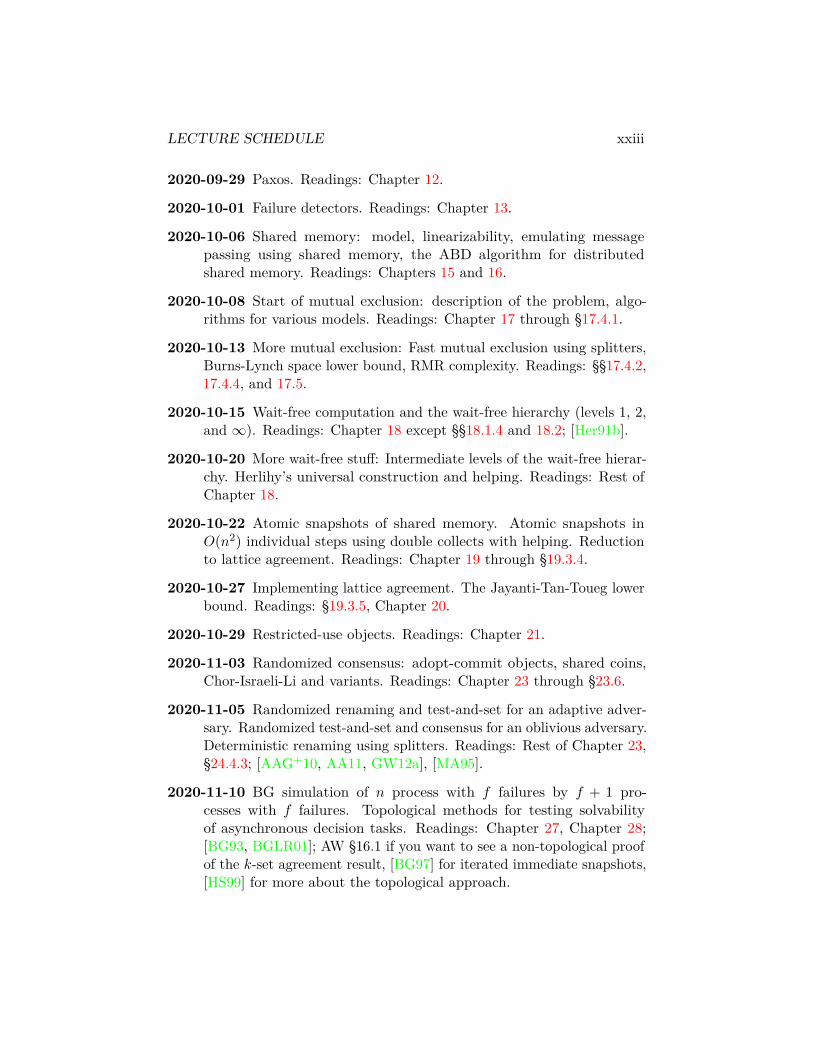
2020-09-29 Paxos. Readings: Chapter 12.

2020-10-01 Failure detectors. Readings: Chapter 13.

2020-10-06 Shared memory: model, linearizability, emulating messagepassing using shared memory, the ABD algorithm for distributedshared memory. Readings: Chapters 15 and 16.

2020-10-08 Start of mutual exclusion: description of the problem, algo-rithms for various models. Readings: Chapter 17 through §17.4.1.

2020-10-13 More mutual exclusion: Fast mutual exclusion using splitters,Burns-Lynch space lower bound, RMR complexity. Readings: §§17.4.2,17.4.4, and 17.5.

2020-10-15 Wait-free computation and the wait-free hierarchy (levels 1, 2,and ∞). Readings: Chapter 18 except §§18.1.4 and 18.2; [Her91b].

2020-10-20 More wait-free stuff: Intermediate levels of the wait-free hierar-chy. Herlihy’s universal construction and helping. Readings: Rest ofChapter 18.

2020-10-22 Atomic snapshots of shared memory. Atomic snapshots inO(n2) individual steps using double collects with helping. Reductionto lattice agreement. Readings: Chapter 19 through §19.3.4.

2020-10-27 Implementing lattice agreement. The Jayanti-Tan-Toueg lowerbound. Readings: §19.3.5, Chapter 20.

2020-10-29 Restricted-use objects. Readings: Chapter 21.

2020-11-03 Randomized consensus: adopt-commit objects, shared coins,Chor-Israeli-Li and variants. Readings: Chapter 23 through §23.6.

2020-11-05 Randomized renaming and test-and-set for an adaptive adver-sary. Randomized test-and-set and consensus for an oblivious adversary.Deterministic renaming using splitters. Readings: Rest of Chapter 23,§24.4.3; [AAG+10, AA11, GW12a], [MA95].

2020-11-10 BG simulation of n process with f failures by f + 1 pro-cesses with f failures. Topological methods for testing solvabilityof asynchronous decision tasks. Readings: Chapter 27, Chapter 28;[BG93, BGLR01]; AW §16.1 if you want to see a non-topological proofof the k-set agreement result, [BG97] for iterated immediate snapshots,[HS99] for more about the topological approach.

LECTURE SCHEDULE xxiv

2020-11-12 Self-stabilization and local computation: Dijkstra’s token ringcirculation algorithm, self-stabilizing synchronizers and BFS trees,relation between local algorithms and self-stabilization. Readings:Chapter 31; [Dij74, AKM+93, LSW09].

2020-11-17 Distributed graph algorithms. The LOCAL and CONGESTmodels. Local graph coloring. Readings: Chapter 32.

2020-11-19 Population protocols. Readings: Chapter 33.

2020-12-01 CPSC 565 student presentations. See §A.6.

2020-12-03 CPSC 565 student presentations.

Chapter 1

Introduction

Distributed systems are characterized by their structure: a typical dis-tributed system will consist of some large number of interacting devices thateach run their own programs but that are affected by receiving messages, orobserving shared-memory updates or the states of other devices. Examplesof distributed systems range from simple systems in which a single clienttalks to a single server to huge amorphous networks like the Internet as awhole.

As distributed systems get larger, it becomes harder and harder topredict or understand their behavior. Part of the reason for this is thatwe as programmers have not yet developed a standardized set of tools formanaging complexity (like subroutines or objects with narrow interfaces,or even simple structured programming mechanisms like loops or if/thenstatements) as are found in sequential programming. Part of the reason isthat large distributed systems bring with them large amounts of inherentnondeterminism—unpredictable events like delays in message arrivals, thesudden failure of components, or in extreme cases the nefarious actions offaulty or malicious machines opposed to the goals of the system as a whole.Because of the unpredictability and scale of large distributed systems, it canoften be difficult to test or simulate them adequately. Thus there is a needfor theoretical tools that allow us to prove properties of these systems thatwill let us use them with confidence.

The first task of any theory of distributed systems is modeling: defininga mathematical structure that abstracts out all relevant properties of a largedistributed system. There are many foundational models in the literature fordistributed systems, but for this class we will follow [AW04] and use simpleautomaton-based models.

1

CHAPTER 1. INTRODUCTION 2

What this means is that we model each process in the system as anautomaton that has some sort of local state, and model local computationas a transition rule that tells us how to update this state in response tovarious events. Depending on what kinds of system we are modeling, theseevents might correspond to local computation, to delivery of a message by anetwork, carrying out some operation on a shared memory, or even somethinglike a chemical reaction between two molecules. The transition rule for asystem specifies how the states of all processes involved in the event areupdated, based on their previous states. We can think of the transitionrule as an arbitrary mathematical function (or relation if the processes arenondeterministic); this corresponds in programming terms to implementinglocal computation by processes as a gigantic table lookup.

Obviously this is not how we program systems in practice. But what thisapproach does is allow us to abstract away completely from how individualprocesses work, and emphasize how all of the processes interact with eachother. This can lead to odd results: for example, it’s perfectly consistentwith this model for some process to be able to solve the halting problem, orcarry out arbitrarily complex calculations between receiving a message andsending its response. A partial justification for this assumption is that inpractice, the multi-millisecond latencies in even reasonably fast networks areeons in terms of local computation. And as with any assumption, we canalways modify it if it gets us into trouble.

1.1 ModelsThe global state consisting of all process states is called a configuration,and we think of the system as a whole as passing from one global stateor configuration to another in response to each event. When this occursthe processes participating in the event update their states, and the otherprocesses do nothing. This does not model concurrency directly; instead,we interleave potentially concurrent events in some arbitrary way. Theadvantage of this interleaving approach is that it gives us essentially thesame behavior as we would get if we modeled simultaneous events explicitly,but still allows us to consider only one event at a time and use induction toprove various properties of the sequence of configurations we might reach.

We will often use lowercase Greek letters for individual events or sequencesof events. Configurations are typically written as capital Latin letters (oftenC). An execution of a schedule is an alternating sequence of configurationsand events C0σ0C1σ1C2 . . . , where Ci+1 is the configuration that results from

CHAPTER 1. INTRODUCTION 3

applying event σi to configuration C. A schedule is a sequence of eventsσ0σ1 . . . from some execution. We say that an event σ is enabled in C ifthis event can be carried out in C; an example would be that the event thatwe deliver a particular message in a message-passing system is enabled onlyif that message has been sent and not yet delivered. When σ is enabled inC, it is sometime convenient to write Cσ for the configuration that resultsfrom applying σ to C.

What events are available, and what effects they have, will dependon what kind of model we are considering. We may also have additionalconstraints on what kinds of schedules are admissible, which restricts theschedules under consideration to those that have certain desirable properties(say, every message that is sent is eventually delivered). There are manymodels in the distributed computing literature, which can be divided into ahandful of broad categories:

• Message passing models (which we will cover in Part I) correspondto systems where processes communicate by sending messages througha network. In synchronous message-passing, every process sendsout messages at time t that are delivered at time t+ 1, at which pointmore messages are sent out that are delivered at time t + 2, and soon: the whole system runs in lockstep, marching forward in perfectsynchrony.1 Such systems are difficult to build when the componentsbecome too numerous or too widely dispersed, but they are ofteneasier to analyze than asynchronous systems, where messages areonly delivered eventually after some unknown delay. Variants on thesemodels include semi-synchronous systems, where message delays areunpredictable but bounded, and various sorts of timed systems. Furthervariations come from restricting which processes can communicate withwhich others, by allowing various sorts of failures: crash failuresthat stop a process dead, Byzantine failures that turn a processevil, or omission failures that drop messages in transit. Or—on thehelpful side—we may supply additional tools like failure detectors(Chapter 13) or randomization (Chapter 23).

• Shared-memory models (Part II) correspond to systems where pro-cesses communicate by executing operations on shared objects

1In an interleaving model, these apparently simultaneous events are still recorded oneat a time. What makes the system synchronous is that we demand that, in any admissibleschedule, all n events for time t occur as a sequential block, followed by all n events fortime t+ 1, and so on.

CHAPTER 1. INTRODUCTION 4

In the simplest case, the objects are simple memory cells supportingread and write operations. These are called atomic registers. Butin general, the objects could be more complex hardware primitiveslike compare-and-swap (§18.1.3), load-linked/store-conditional(§18.1.3), atomic queues, or even more exotic objects from the seldom-visited theoretical depths.Practical shared-memory systems may be implemented as distributedshared-memory (Chapter 16) on top of a message-passing system.This gives an alternative approach to designing message-passing systemsif it turns out that shared memory is easier to use for a particularproblem.Like message-passing systems, shared-memory systems must also dealwith issues of asynchrony and failures, both in the processes and in theshared objects.Realistic shared-memory systems have additional complications, in thatmodern CPUs allow out-of-order execution in the absence of special(and expensive) operations called fences or memory barriers.[AG95]We will effectively be assuming that our shared-memory code is liberallysprinkled with these operations so that nothing surprising happens,but this is not always true of real production code, and indeed there iswork in the theory of distributed computing literature on algorithmsthat don’t require unlimited use of memory barriers.

• A third family of models has no communication mechanism indepen-dent of the processes. Instead, the processes may directly observethe states of other processes. These models are used in analyzingself-stabilization, for some biologically inspired systems, andfor computation by population protocols or chemical reactionnetworks. We will discuss some of this work in Part III.

• Other specialized models emphasize particular details of distributedsystems, such as the labeled-graph models used for analyzing routing orthe topological models used to give a very high-level picture of variousdistributed decision problems (see Chapter 28).

We’ll see many of these at some point in this course, and examine whichof them can simulate each other under various conditions.

CHAPTER 1. INTRODUCTION 5

1.2 PropertiesProperties we might want to prove about a system include:

• Safety properties, of the form “nothing bad ever happens” or, moreprecisely, “there are no bad reachable configurations.” These includethings like “at most one of the traffic lights at the intersection of BusyRoad and Main Street is ever green” or “every value read from a counterequals the number of preceding increment operations.” Such propertiesare typically proved using an , a property of configurations that is trueinitially and that is preserved by all transitions (this is essentially adisguised induction proof).

• Liveness properties, of the form “something good eventually happens.”An example might be “my email is eventually either delivered orreturned to me.” These are not properties of particular states (I mightunhappily await the eventual delivery of my email for decades withoutviolating the liveness property just described), but of executions, wherethe property must hold starting at some finite time. Liveness propertiesare generally proved either from other liveness properties (e.g., “allmessages in this message-passing system are eventually delivered”)or from a combination of such properties and some sort of timerargument where some progress metric improves with every transitionand guarantees the desirable state when it reaches some bound (also adisguised induction proof).

• Fairness properties are a strong kind of liveness property of the form“something good eventually happens to everybody.” Such propertiesexclude starvation, a situation where most of the kids are happilychowing down at the orphanage (“some kid eventually eats something”is a liveness property) but poor Oliver Twist is dying in the corner forlack of gruel.

• Simulations show how to build one kind of system from another,such as a reliable message-passing system built on top of an unreliablesystem (TCP [Pos81]), a shared-memory system built on top of amessage-passing system (distributed shared memory—see Chapter 16),or a synchronous system build on top of an asynchronous system(synchronizers—see Chapter 7).

• Impossibility results describe things we can’t do. For example, theclassic Two Generals impossibility result (Chapter 8) says that it’s

CHAPTER 1. INTRODUCTION 6

impossible to guarantee agreement between two processes across anunreliable message-passing channel if even a single message can belost. Other results characterize what problems can be solved if variousfractions of the processes are unreliable, or if asynchrony makes timingassumptions impossible. These results, and similar lower bounds thatdescribe things we can’t do quickly, include some of the most technicallysophisticated results in distributed computing. They stand in contrastto the situation with sequential computing, where the reliability andpredictability of the underlying hardware makes proving lower boundsextremely difficult.

There are some basic proof techniques that we will see over and overagain in distributed computing.

For lower bound and impossibility proofs, the main tool is the in-distinguishability argument. Here we construct two (or more) executionsin which some process has the same input and thus behaves the same way,regardless of what algorithm it is running. This exploitation of process’s ig-norance is what makes impossibility results possible in distributed computingdespite being notoriously difficult in most areas of computer science.2

For safety properties, statements that some bad outcome never occurs,the main proof technique is to construct an invariant. An invariant isessentially an induction hypothesis on reachable configurations of the system;an invariant proof shows that the invariant holds in all initial configurations,and that if it holds in some configuration, it holds in any configuration thatis reachable in one step.

Induction is also useful for proving termination and liveness properties,statements that some good outcome occurs after a bounded amount of time.Here we typically structure the induction hypothesis as a progress measure,showing that some sort of partial progress holds by a particular time, withthe full guarantee implied after the time bound is reached.

2An exception might be lower bounds for data structures, which also rely on a process’signorance.

Part I

Message passing

7

Chapter 2

Model

Message passing models simulate networks. Because any interaction betweenphysically separated processors requires transmitting information from oneplace to another, all distributed systems are, at a low enough level, message-passing systems. We start by defining a formal model of these systems.

2.1 Basic message-passing modelWe have a collection of n processes p1 . . . p2, each of which has a stateconsisting of a state from from state set Qi. We think of these processesas nodes in a directed communication graph or network. The edges inthis graph are a collection of point-to-point channels or buffers bij , onefor each pair of adjacent processes i and j, representing messages that havebeen sent but that have not yet been delivered. Implicit in this definition isthat messages are point-to-point, with a single sender and recipient: if youwant broadcast, you have to build it yourself.

A configuration of the system consists of a vector of states, one for eachprocess and channel. The configuration of the system is updated by an event,in which (1) zero or more messages in channels bij are delivered to process pj ,removing them from bij ; (2) pj updates its state in response; and (3) zero ormore messages are added by pj to outgoing channels bji. We generally thinkof these events as delivery events when at least one message is delivered,and as computation events when none are. An execution segment is asequence of alternating configurations and events C0, φ1, C1, φ2, . . . , in whicheach triple Ciφi+1Ci+1 is consistent with the transition rules for the eventφi+1, and the last element of the sequence (if any) is a configuration. If thefirst configuration C0 is an initial configuration of the system, we have an

8

CHAPTER 2. MODEL 9

execution. A schedule is an execution with the configurations removed.

2.1.1 Formal details

Let P be the set of processes, Q the set of process states, and M the set ofpossible messages.

Each process pi has a state statei ∈ Q. Each channel bij has a statebufferij ∈ P(M). We assume each process has a transition functionδ : Q× P(M)→ Q× P(P ×M) that maps tuples consisting of a state anda set of incoming messages a new state and a set of recipients and messagesto be sent. An important feature of the transition function is that theprocess’s behavior can’t depend on which of its previous messages have beendelivered or not. A delivery event del(i, A), where A = (jk,mk)) removeseach message mk from bji, updates statei according to δ(statei, A), and addsthe outgoing messages specified to δ(statei, A) to the appropriate channels.A computation event comp(i) does the same thing, except that it appliesδ(statej , ∅).

Some implicit features in this definition:

• A process can’t tell when its outgoing messages are delivered, becausethe channel states aren’t available as input to δ.

• Processes are deterministic: The next action of each process dependsonly on its current state, and not on extrinsic variables like the phaseof the moon, coin-flips, etc. We may wish to relax this condition laterby allowing coin-flips; to do so, we will need to extend the model toincorporate probabilities.

• It is possible to determine the accessible state of a process by lookingonly at events that involve that process. Specifically, given a scheduleS, define the restriction S|i to be the subsequence consisting of allcomp(i) and del(i, A) events (ranging over all possible A). Since theseare the only events that affect the state of i, and only the state of i isneeded to apply the transition function, we can compute the state of ilooking only at S|i. In particular, this means that i will have the sameaccessible state after any two schedules S and S′ where S|i = S′|i, andthus will take the same actions in both schedules. This is the basis forindistinguishability proofs (§8.2), a central technique in obtaininglower bounds and impossibility results.

Attiya and Welch [AW04] use a different model in which communicationchannels are not modeled separately from processes, but instead are baked

CHAPTER 2. MODEL 10

into processes as outbuf and inbuf variables. This leads to some oddities likehaving to distinguish the accessible state of a process (which excludes theoutbufs) from the full state (which doesn’t). Our approach is close to that ofLynch [Lyn96], in that we have separate automata representing processes andcommunication channels. But since the resulting model produces essentiallythe same executions, the exact details don’t really matter.1

2.1.2 Network structure

It may be the case that not all processes can communicate directly; if so,we impose a network structure in the form of a directed graph, where i cansend a message to j if and only if there is an edge from i to j in the graph.Typically we assume that each process knows the identity of all its neighbors.

For some problems (e.g., in peer-to-peer systems or other overlay net-works) it may be natural to assume that there is a fully-connected underlyingnetwork but that we have a dynamic network on top of it, where processescan only send to other processes that they have obtained the addresses of insome way.

2.2 Asynchronous systemsIn an asynchronous model, only minimal restrictions are placed on whenmessages are delivered and when local computation occurs. A schedule issaid to be admissible if (a) there are infinitely many computation stepsfor each process, and (b) every message is eventually delivered. (These arefairness conditions.) The first condition (a) assumes that processes do notexplicitly terminate, which is the assumption used in [AW04]; an alternative,which we will use when convenient, is to assume that every process eitherhas infinitely many computation steps or reaches an explicit halting state.

1The late 1970s and early 1980s saw a lot of research on finding the “right” definitionof a distributed system, and some of the disputes from that era were hard fought. But inthe end, all the various proposed models turned out to be more or less equivalent, whichis not surprising since the authors were ultimately trying to represent the same intuitiveunderstanding of these systems. So most distributed computing papers now just use somephrasing like “we consider the standard model of an asynchronous message-passing system”and leave it to the reader to assume that this standard model is their favorite one.An example of this trick in action is that you will never see del(i, A) or comp(i) again

after you finish reading this footnote.

CHAPTER 2. MODEL 11

2.2.1 Example: client-server computing

Almost every distributed system in practical use is based on client-serverinteractions. Here one process, the client, sends a request to a secondprocess, the server, which in turn sends back a response. We can modelthis interaction using our asynchronous message-passing model by describingwhat the transition functions for the client and the server look like: seeAlgorithms 2.1 and 2.2.

1 initially do2 send request to server

Algorithm 2.1: Client-server computation: client code

1 upon receiving request do2 send response to client

Algorithm 2.2: Client-server computation: server code

The interpretation of Algorithm 2.1 is that the client sends request (byadding it to its outbuf) in its very first computation event (after which it doesnothing). The interpretation of Algorithm 2.2 is that in any computationevent where the server observes request in its inbuf, it sends response.

We want to claim that the client eventually receives response in anyadmissible execution. To prove this, observe that:

1. After finitely many steps, the client carries out a computation event.This computation event puts request in its outbuf.

2. After finitely many more steps, a delivery event occurs that deliversrequest to the server. This causes the server to send response.

3. After finitely many more steps, a delivery event delivers response tothe client, causing it to process response (and do nothing, given thatwe haven’t included any code to handle this response).

Each step of the proof is justified by the constraints on admissibleexecutions. If we could run for infinitely many steps without a particularprocess doing a computation event or a particular message being delivered,we’d violate those constraints.

Most of the time we will not attempt to prove the correctness of aprotocol at quite this level of tedious detail. But if you are only interested in

CHAPTER 2. MODEL 12

distributed algorithms that people actually use, you have now seen a proofof correctness for 99.9% of them, and do not need to read any further.

2.3 Synchronous systemsA synchronous message-passing system is exactly like an asynchronoussystem, except we insist that the schedule consists of alternating phases inwhich (a) every process executes a computation step, and (b) all messagesare delivered while none are sent.2 The combination of a computation phaseand a delivery phase is called a round. Synchronous systems are effectivelythose in which all processes execute in lock-step, and there is no timinguncertainty. This makes protocols much easier to design, but makes themless resistant to real-world timing oddities. Sometimes this can be dealt withby applying a synchronizer (Chapter 7), which transforms synchronousprotocols into asynchronous protocols at a small cost in complexity.

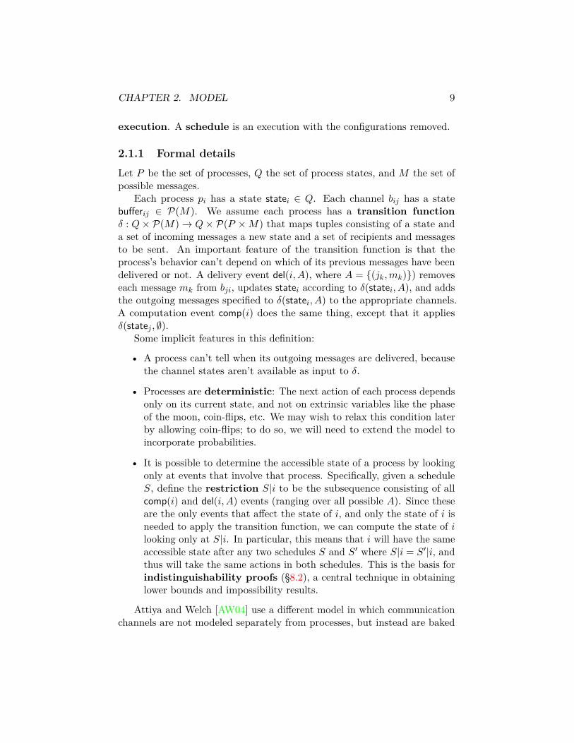
2.4 Drawing message-passing executionsThough formally we can describe an execution in a message-passing systemas a long list of events, this doesn’t help much with visualizing the underlyingcommunication pattern. So it can sometimes be helpful to use a more visualrepresentation of a message-passing execution that shows how informationflows through the system.

A typical example is given in Figure 2.1. In this picture, time flowsfrom left to right, and each process is represented by a horizontal line. Thisconvention reflects the fact that processes have memory, so any informationavailable to a process at some time t is also available at all times t′ ≥ t.Events are represented by marked points on these lines, and messages arerepresented by diagonal lines between events. The resulting picture looks likea collection of world lines as used in physics to illustrate the path takenby various objects through spacetime.

Pictures like Figure 2.1 can be helpful for illustrating the various con-straints we might put on message delivery. In Figure 2.1, the system iscompletely asynchronous: messages can be delivered in any order, even ifsent between the same processes. If we run the same protocol under strongerassumptions, we will get different communication patterns.

2Formally, the delivery phase consists of n separate delivery events, in any order, thatbetween them clean out all the channels.

CHAPTER 2. MODEL 13

p1

p2

p3

Time →

Figure 2.1: Asynchronous message-passing execution. Time flows left-to-right. Horizontal lines represent processes. Nodes represent events. Diagonaledges between events represent messages. In this execution, p1 executes acomputation event that sends messages to p2 and p3. When p2 receives thismessage, it sends messages to p1 and p3. Later, p2 executes a computationevent that sends a second message to p1. Because the system is asynchronous,there is no guarantee that messages arrive in the same order they are sent.

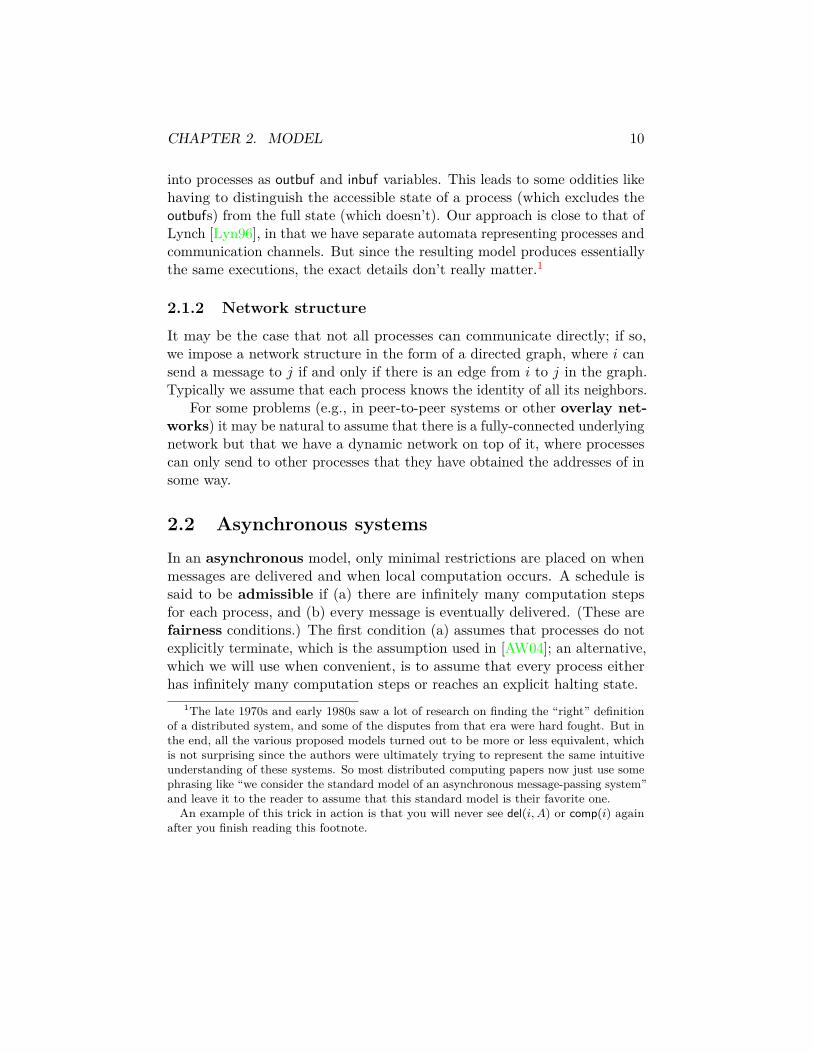
For example, Figure 2.2 shows an execution that is still asynchronous butthat assumes FIFO (first-in first-out) channels. A FIFO channel from someprocess p to another process q guarantees that q receives messages in thesame order that p sends them (this can be simulated by a non-FIFO channelby adding a sequence number to each message, and queuing messages atthe receiver until all previous messages have been processed).

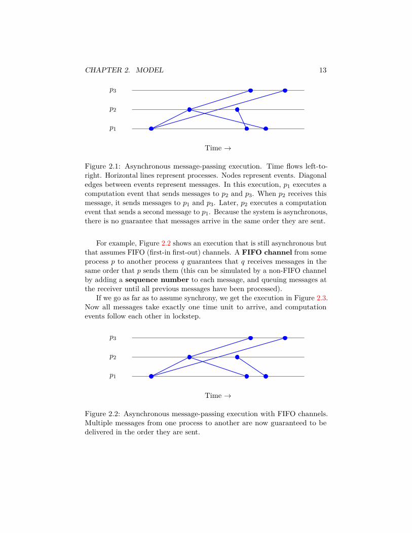
If we go as far as to assume synchrony, we get the execution in Figure 2.3.Now all messages take exactly one time unit to arrive, and computationevents follow each other in lockstep.

p1

p2

p3

Time →

Figure 2.2: Asynchronous message-passing execution with FIFO channels.Multiple messages from one process to another are now guaranteed to bedelivered in the order they are sent.

CHAPTER 2. MODEL 14

p1

p2

p3

Time →

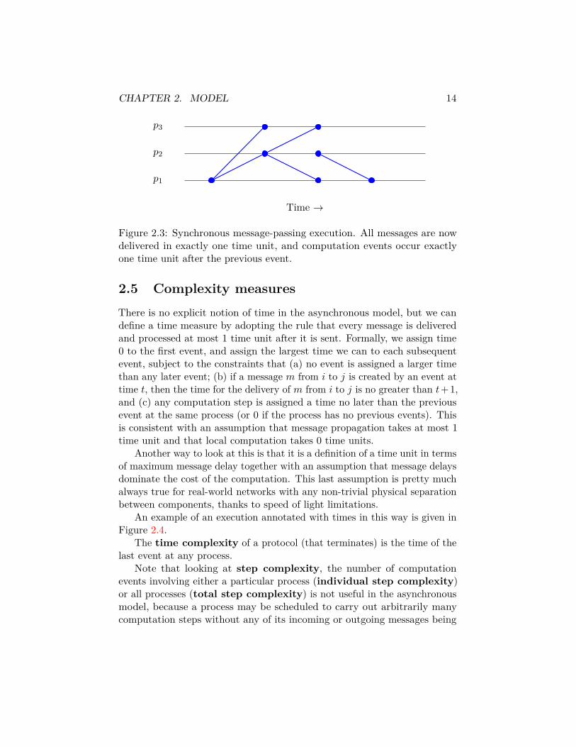
Figure 2.3: Synchronous message-passing execution. All messages are nowdelivered in exactly one time unit, and computation events occur exactlyone time unit after the previous event.

2.5 Complexity measuresThere is no explicit notion of time in the asynchronous model, but we candefine a time measure by adopting the rule that every message is deliveredand processed at most 1 time unit after it is sent. Formally, we assign time0 to the first event, and assign the largest time we can to each subsequentevent, subject to the constraints that (a) no event is assigned a larger timethan any later event; (b) if a message m from i to j is created by an event attime t, then the time for the delivery of m from i to j is no greater than t+ 1,and (c) any computation step is assigned a time no later than the previousevent at the same process (or 0 if the process has no previous events). Thisis consistent with an assumption that message propagation takes at most 1time unit and that local computation takes 0 time units.

Another way to look at this is that it is a definition of a time unit in termsof maximum message delay together with an assumption that message delaysdominate the cost of the computation. This last assumption is pretty muchalways true for real-world networks with any non-trivial physical separationbetween components, thanks to speed of light limitations.

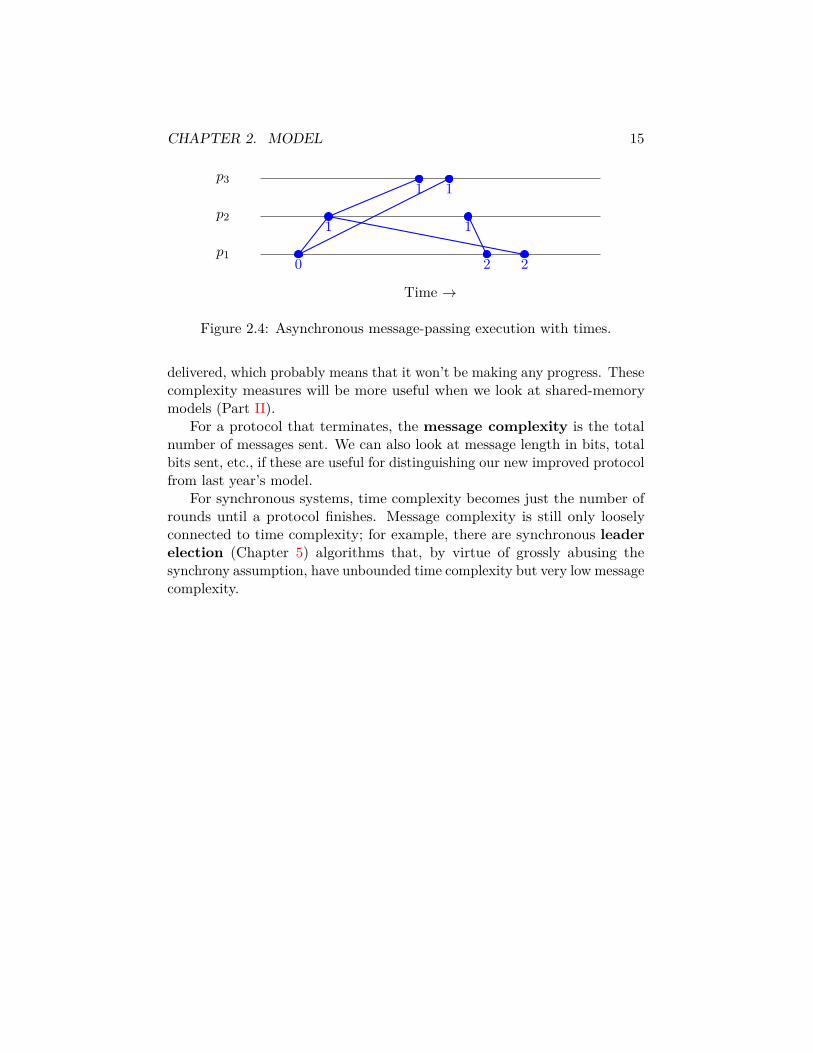
An example of an execution annotated with times in this way is given inFigure 2.4.

The time complexity of a protocol (that terminates) is the time of thelast event at any process.

Note that looking at step complexity, the number of computationevents involving either a particular process (individual step complexity)or all processes (total step complexity) is not useful in the asynchronousmodel, because a process may be scheduled to carry out arbitrarily manycomputation steps without any of its incoming or outgoing messages being

CHAPTER 2. MODEL 15

p1

p2

p3

Time →

0

1

1

2

1

2

1

Figure 2.4: Asynchronous message-passing execution with times.

delivered, which probably means that it won’t be making any progress. Thesecomplexity measures will be more useful when we look at shared-memorymodels (Part II).

For a protocol that terminates, the message complexity is the totalnumber of messages sent. We can also look at message length in bits, totalbits sent, etc., if these are useful for distinguishing our new improved protocolfrom last year’s model.

For synchronous systems, time complexity becomes just the number ofrounds until a protocol finishes. Message complexity is still only looselyconnected to time complexity; for example, there are synchronous leaderelection (Chapter 5) algorithms that, by virtue of grossly abusing thesynchrony assumption, have unbounded time complexity but very low messagecomplexity.

Chapter 3

Broadcast and convergecast

Here we’ll describe protocols for propagating information throughout anetwork from some central initiator and gathering information back to thatsame initiator. We do this both because the algorithms are actually usefuland because they illustrate some of the issues that come up with keepingtime complexity down in an asynchronous message-passing system.

3.1 FloodingFlooding is about the simplest of all distributed algorithms. It’s dumb andexpensive, but easy to implement, and gives you both a broadcast mechanismand a way to build rooted spanning trees.

We’ll give a fairly simple presentation of flooding roughly followingChapter 2 of [AW04].

3.1.1 Basic algorithm

The basic flooding algorithm is shown in Algorithm 3.1. The idea is thatwhen a process receives a message M , it forwards it to all of its neighborsunless it has seen it before, which it tracks using a single bit seen-message.

Theorem 3.1.1. Every process receives M after at most D time and atmost |E| messages, where D is the diameter of the network and E is the setof (directed) edges in the network.

Proof. Message complexity: Each process only sends M to its neighborsonce, so each edge carries at most one copy of M .

Time complexity: By induction on d(root, v), we’ll show that each vreceives M for the first time no later than time d(root, v) ≤ D. The base

16

CHAPTER 3. BROADCAST AND CONVERGECAST 17

1 initially do2 if pid = root then3 seen-message← true4 send M to all neighbors5 else6 seen-message← false

7 upon receiving M do8 if seen-message = false then9 seen-message← true

10 send M to all neighbors

Algorithm 3.1: Basic flooding algorithm

case is when v = root, d(root, v) = 0; here root receives message at time0. For the induction step, Let d(root, v) = k > 0. Then v has a neighboru such that d(root, u) = k − 1. By the induction hypothesis, u receives Mfor the first time no later than time k − 1. From the code, u then sendsM to all of its neighbors, including v; M arrives at v no later than time(k − 1) + 1 = k.

Note that the time complexity proof also demonstrates correctness: everyprocess receives M at least once.

As written, this is a one-shot algorithm: you can’t broadcast a secondmessage even if you wanted to. The obvious fix is for each process toremember which messages it has seen and only forward the new ones (whichcosts memory) and/or to add a time-to-live (TTL) field on each messagethat drops by one each time it is forwarded (which may cost extra messagesand possibly prevents complete broadcast if the initial TTL is too small).The latter method is what was used for searching in http://en.wikipedia.org/wiki/Gnutella, an early peer-to-peer system. An interesting propertyof Gnutella was that since the application of flooding was to search for huge(multiple MiB) files using tiny ( 100 byte) query messages, the actual bitcomplexity of the flooding algorithm was not especially large relative to thebit complexity of sending any file that was found.

We can optimize the algorithm slightly by not sending M back to thenode it came from; this will slightly reduce the message complexity in manycases but makes the proof a sentence or two longer. (It’s all a question ofwhat you want to optimize.)

CHAPTER 3. BROADCAST AND CONVERGECAST 18

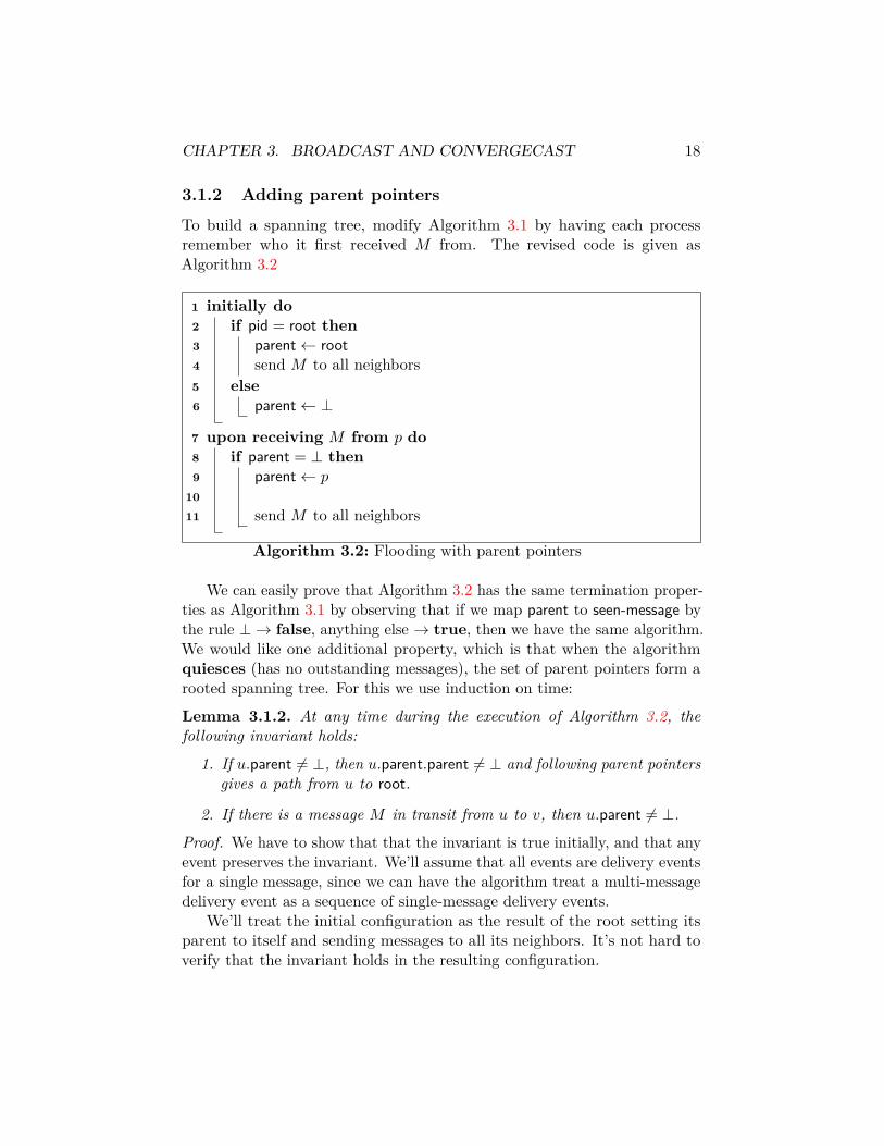
3.1.2 Adding parent pointers

To build a spanning tree, modify Algorithm 3.1 by having each processremember who it first received M from. The revised code is given asAlgorithm 3.2

1 initially do2 if pid = root then3 parent← root4 send M to all neighbors5 else6 parent← ⊥

7 upon receiving M from p do8 if parent = ⊥ then9 parent← p

1011 send M to all neighbors

Algorithm 3.2: Flooding with parent pointers

We can easily prove that Algorithm 3.2 has the same termination proper-ties as Algorithm 3.1 by observing that if we map parent to seen-message bythe rule ⊥ → false, anything else → true, then we have the same algorithm.We would like one additional property, which is that when the algorithmquiesces (has no outstanding messages), the set of parent pointers form arooted spanning tree. For this we use induction on time:

Lemma 3.1.2. At any time during the execution of Algorithm 3.2, thefollowing invariant holds:

1. If u.parent 6= ⊥, then u.parent.parent 6= ⊥ and following parent pointersgives a path from u to root.

2. If there is a message M in transit from u to v, then u.parent 6= ⊥.

Proof. We have to show that that the invariant is true initially, and that anyevent preserves the invariant. We’ll assume that all events are delivery eventsfor a single message, since we can have the algorithm treat a multi-messagedelivery event as a sequence of single-message delivery events.

We’ll treat the initial configuration as the result of the root setting itsparent to itself and sending messages to all its neighbors. It’s not hard toverify that the invariant holds in the resulting configuration.

CHAPTER 3. BROADCAST AND CONVERGECAST 19

For a delivery event, let v receive M from u. There are two cases: ifv.parent is already non-null, the only state change is that M is no longer intransit, so we don’t care about u.parent any more. If v.parent is null, then

1. v.parent is set to u. This triggers the first case of the invariant. Fromthe induction hypothesis we have that u.parent 6= ⊥ and that thereexists a path from u to the root. Then v.parent.parent = u.parent 6= ⊥and the path from v → u→ root gives the path from v.

2. Message M is sent to all of v’s neighbors. Because M is now in transitfrom v, we need v.parent 6= ⊥; but we just set it to u, so we are happy.

At the end of the algorithm, the invariant shows that every process has apath to the root, i.e., that the graph represented by the parent pointers isconnected. Since this graph has exactly |V | − 1 edges (if we don’t count theself-loop at the root), it’s a tree.

Though we get a spanning tree at the end, we may not get a very goodspanning tree. For example, suppose our friend the adversary picks someHamiltonian path through the network and delivers messages along thispath very quickly while delaying all other messages for the full allowed 1time unit. Then the resulting spanning tree will have depth |V | − 1, whichmight be much worse than D. If we want the shallowest possible spanningtree, we need to do something more sophisticated: see the discussion ofdistributed breadth-first search in Chapter 4. However, we may behappy with the tree we get from simple flooding: if the message delay oneach link is consistent, then it’s not hard to prove that we in fact get ashortest-path tree. As a special case, flooding always produces a BFS tree inthe synchronous model.

Note also that while the algorithm works in a directed graph, the parentpointers may not be very useful if links aren’t two-way.

3.1.3 Termination

See [AW04, Chapter 2] for further modifications that allow the processes todetect termination. In a sense, each process can terminate as soon as it isdone sendingM to all of its neighbors, but this still requires some mechanismfor clearing out the inbuf; by adding acknowledgments as described in [AW04],we can terminate with the assurance that no further messages will be received.

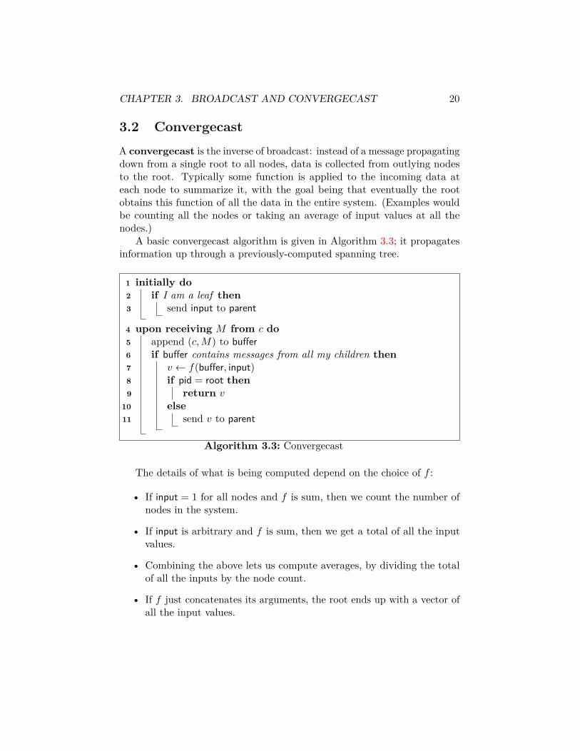
CHAPTER 3. BROADCAST AND CONVERGECAST 20

3.2 ConvergecastA convergecast is the inverse of broadcast: instead of a message propagatingdown from a single root to all nodes, data is collected from outlying nodesto the root. Typically some function is applied to the incoming data ateach node to summarize it, with the goal being that eventually the rootobtains this function of all the data in the entire system. (Examples wouldbe counting all the nodes or taking an average of input values at all thenodes.)

A basic convergecast algorithm is given in Algorithm 3.3; it propagatesinformation up through a previously-computed spanning tree.

1 initially do2 if I am a leaf then3 send input to parent

4 upon receiving M from c do5 append (c,M) to buffer6 if buffer contains messages from all my children then7 v ← f(buffer, input)8 if pid = root then9 return v

10 else11 send v to parent

Algorithm 3.3: Convergecast

The details of what is being computed depend on the choice of f :

• If input = 1 for all nodes and f is sum, then we count the number ofnodes in the system.

• If input is arbitrary and f is sum, then we get a total of all the inputvalues.

• Combining the above lets us compute averages, by dividing the totalof all the inputs by the node count.

• If f just concatenates its arguments, the root ends up with a vector ofall the input values.

CHAPTER 3. BROADCAST AND CONVERGECAST 21

Running time is bounded by the depth of the tree: we can prove byinduction that any node at height h (height is length of the longest path fromthis node to some leaf) sends a message by time h at the latest. Messagecomplexity is exactly n− 1, where n is the number of nodes; this is easilyshown by observing that each node except the root sends exactly one message.

Proving that convergecast returns the correct value is similarly done byinduction on depth: if each child of some node computes a correct value, thenthat node will compute f applied to these values and its own input. Whatthe result of this computation is will, of course, depend on f ; it generallymakes the most sense when f represents some associative operation (as inthe examples above).

3.3 Flooding and convergecast togetherA natural way to build the spanning tree used by convergecast is to runflooding first. This also provides a mechanism for letting the leaves knowthat they are leaves and initiating the protocol. The combined algorithm isshown as Algorithm 3.4.

However, this may lead to very bad time complexity for the convergecaststage. Consider a wheel-shaped network consisting of one central node p0connected to nodes p1, p2, . . . , pn−1, where each pi is also connected to pi+1.By carefully arranging for the pipi+1 links to run much faster than the p0pilinks, the adversary can make flooding build a tree that consists of a singlepath p0p1p2 . . . pn−1, even though the diameter of the network is only 2.While it only takes 2 time units to build this tree (because every node is onlyone hop away from the initiator), when we run convergecast we suddenlyfind that the previously-speedy links are now running only at the guaranteed≤ 1 time unit per hop rate, meaning that convergecast takes n− 1 time.

This may be less of an issue in real networks, where the latency of linksmay be more uniform over time, meaning that a deep tree of fast links isstill likely to be fast when we reach the convergecast step. But in the worstcase we will need to be more clever about building the tree. We show howto do this in Chapter 4.

CHAPTER 3. BROADCAST AND CONVERGECAST 22

1 initially do2 children← ∅3 nonChildren← ∅4 if pid = root then5 parent← root6 send init to all neighbors7 else8 parent← ⊥

9 upon receiving init from p do10 if parent = ⊥ then11 parent← p12 send init to all neighbors13 else14 send nack to p

15 upon receiving nack from p do16 nonChildren← nonChildren ∪ p17 as soon as children ∪ nonChildren includes all my neighbors do18 v ← f(buffer, input)19 if pid = root then20 return v21 else22 send ack(v) to parent

23 upon receiving ack(v) from k do24 add (k, v) to buffer25 add k to children

Algorithm 3.4: Flooding and convergecast combined

Chapter 4

Distributed breadth-firstsearch

Here we describe some algorithms for building a breadth-first search(BFS) tree in a network. All assume that there is a designated initiatornode that starts the algorithm. At the end of the execution, each node exceptthe initiator has a parent pointer and every node has a list of children. Theseare consistent and define a BFS tree: nodes at distance k from the initiatorappear at level k of the tree.

In a synchronous network, flooding (§3.1) solves BFS; see [AW04,Lemma 2.8, page 21] or [Lyn96, §4.2]. So the interesting case is whenthe network is asynchronous.

In an asynchronous network, the complication is that we can no longerrely on synchronous communication to reach all nodes at distance d at thesame time. So instead we need to keep track of distances explicitly, orpossibly enforce some approximation to synchrony in the algorithm. (Ageneral version of this last approach is to apply a synchronizer to one of thesynchronous algorithms using a synchronizer; see Chapter 7.)

To keep things simple, we’ll drop the requirement that a parent learnthe IDs of its children, since this can be tacked on as a separate notificationprotocol, in which each child just sends one message to its parent once itfigures out who its parent is.

4.1 Using explicit distancesThis is a translation of the AsynchBFS automaton from [Lyn96, §15.4]. It’sa very simple algorithm, closely related to Dijkstra’s algorithm for shortest

23

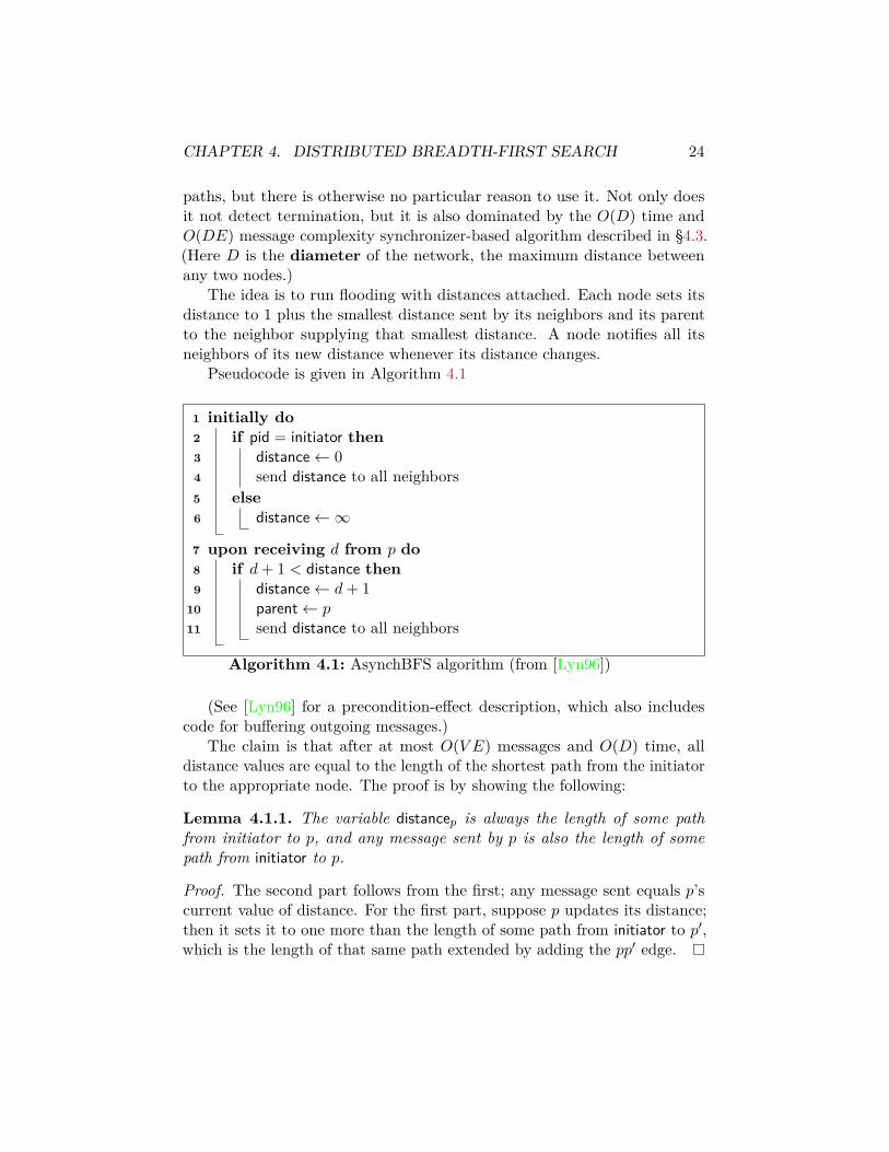
CHAPTER 4. DISTRIBUTED BREADTH-FIRST SEARCH 24

paths, but there is otherwise no particular reason to use it. Not only doesit not detect termination, but it is also dominated by the O(D) time andO(DE) message complexity synchronizer-based algorithm described in §4.3.(Here D is the diameter of the network, the maximum distance betweenany two nodes.)

The idea is to run flooding with distances attached. Each node sets itsdistance to 1 plus the smallest distance sent by its neighbors and its parentto the neighbor supplying that smallest distance. A node notifies all itsneighbors of its new distance whenever its distance changes.

Pseudocode is given in Algorithm 4.1

1 initially do2 if pid = initiator then3 distance← 04 send distance to all neighbors5 else6 distance←∞

7 upon receiving d from p do8 if d+ 1 < distance then9 distance← d+ 1

10 parent← p11 send distance to all neighbors

Algorithm 4.1: AsynchBFS algorithm (from [Lyn96])

(See [Lyn96] for a precondition-effect description, which also includescode for buffering outgoing messages.)

The claim is that after at most O(V E) messages and O(D) time, alldistance values are equal to the length of the shortest path from the initiatorto the appropriate node. The proof is by showing the following:

Lemma 4.1.1. The variable distancep is always the length of some pathfrom initiator to p, and any message sent by p is also the length of somepath from initiator to p.

Proof. The second part follows from the first; any message sent equals p’scurrent value of distance. For the first part, suppose p updates its distance;then it sets it to one more than the length of some path from initiator to p′,which is the length of that same path extended by adding the pp′ edge.

CHAPTER 4. DISTRIBUTED BREADTH-FIRST SEARCH 25

We also need a liveness argument that says that distancep = d(initiator, p)no later than time d(initiator, p). Note that we can’t detect when distancestabilizes to the correct value without a lot of additional work.

In [Lyn96], there’s an extra |V | term in the time complexity that comesfrom message pile-ups, since the model used there only allows one incomingmessage to be processed per time units (the model in [AW04] doesn’t havethis restriction). The trick to arranging this to happen often is to build agraph where node 1 is connected to nodes 2 and 3, node 2 to 3 and 4, node3 to 4 and 5, etc. This allows us to quickly generate many paths of distinctlengths from node 1 to node k, which produces k outgoing messages fromnode k. It may be that a more clever analysis can avoid this blowup, byshowing that it only happens in a few places.

4.2 Using layeringThis approach is used in the LayeredBFS algorithm in [Lyn96], which is dueto Gallager [Gal82].

Here we run a sequence of up to |V | instances of the simple algorithmwith a distance bound on each: instead of sending out just 0, the initiatorsends out (0, bound), where bound is initially 1 and increases at each phase.A process only sends out its improved distance if it is less than bound.

Each phase of the algorithm constructs a partial BFS tree that containsonly those nodes within distance bound of the root. This tree is used toreport back to the root when the phase is complete. For the following phase,notification of the increase in bound increase is distributed only throughthe partial BFS tree constructed so far. With some effort, it is possible toprove that in a bidirectional network that this approach guarantees thateach edge is only probed once with a new distance (since distance-1 nodesare recruited before distance-2 nodes and so on), and the bound-update andacknowledgment messages contribute at most |V | messages per phase. So weget O(E + V D) total messages. But the time complexity is bad: O(D2) inthe worst case.

4.3 Using local synchronizationThe reason the layering algorithm takes so long is that at each phase wehave to phone all the way back up the tree to the initiator to get permissionto go on to the next phase. We need to do this to make sure that a nodeis only recruited into the tree once: otherwise we can get pile-ups on the

CHAPTER 4. DISTRIBUTED BREADTH-FIRST SEARCH 26

channels as in the simple algorithm. But we don’t necessarily need to do thisglobally. Instead, we’ll require each node at distance d to delay sending outa recruiting message until it has confirmed that none of its neighbors will besending it a smaller distance. We do this by having two classes of messages:1

• exactly(d): “I know that my distance is d.”

• more-than(d): “I know that my distance is > d.”

The rules for sending these messages for a non-initiator are:

1. I can send exactly(d) as soon as I have received exactly(d− 1) from atleast one neighbor and more-than(d− 2) from all neighbors.

2. I can sendmore-than(d) if d = 0 or as soon as I have receivedmore-than(d−1) from all neighbors.

The initiator sends exactly(0) to all neighbors at the start of the protocol(these are the only messages the initiator sends).

My distance will be the unique distance that I am allowed to send in anexactly(d) messages. Note that this algorithm terminates in the sense thatevery node learns its distance at some finite time.

If you read the discussion of synchronizers in Chapter 7, this algorithmessentially corresponds to building the alpha synchronizer into the syn-chronous BFS algorithm, just as the layered model builds in the betasynchronizer. See [AW04, §11.3.2] for a discussion of BFS using synchro-nizers. The original approach of applying synchronizers to get BFS is due toAwerbuch [Awe85].

We now show correctness. Under the assumption that local computationtakes zero time and message delivery takes at most 1 time unit, we’ll showthat if d(initiator, p) = d, (a) p sends more-than(d′) for any d′ < d by timed′, (b) p sends exactly(d) by time d, (c) p never sends more-than(d′) for anyd′ ≥ d, and (d) p never sends exactly(d′) for any d′ 6= d. For parts (c) and(d) we use induction on d′; for (a) and (b), induction on time. This is notterribly surprising: (c) and (d) are safety properties, so we don’t need totalk about time. But (a) and (b) are liveness properties so time comes in.

Let’s start with (c) and (d). The base case is that the initiator neversends any more-than messages at all, and so never sends more-than(0), and

1In an earlier version of these notes, these messages where called distance(d) andnot-distance(d); the more self-explanatory exactly and more-than terminology is taken from[BDLP08].

CHAPTER 4. DISTRIBUTED BREADTH-FIRST SEARCH 27

any non-initiator never sends exactly(0). For larger d′, observe that if anon-initiator p sends more-than(d′) for d′ ≥ d, it must first have receivedmore-than(d′ − 1) from all neighbors, including some neighbor p′ at distanced−1. But the induction hypothesis tells us that p′ can’t send more-than(d′−1)for d′ − 1 ≥ d − 1. Similarly, to send exactly(d′) for d′ < d, p must firsthave received exactly(d′ − 1) from some neighbor p′, but again p′ must be atdistance at least d−1 from the initiator and so can’t send this message either.In the other direction, to send exactly(d′) for d′ > d, p must first receivemore-than(d′−2) from this closer neighbor p′, but then d′−2 > d−2 ≥ d−1so more-than(d′ − 2) is not sent by p′.

Now for (a) and (b). The base case is that the initiator sends exactly(0)to all nodes at time 0, giving (a), and there is no more-than(d′) with d′ < 0for it to send, giving (b) vacuously; and any non-initiator sends more-than(0)immediately. At time t+ 1, we have that (a) more-than(t) was sent by anynode at distance t + 1 or greater by time t and (b) exactly(t) was sent byany node at distance t by time t; so for any node at distance t + 2 wesend more-than(t+ 1) no later than time t+ 1 (because we already receivedmore-than(t) from all our neighbors) and for any node at distance t+ 1 wesend exactly(t + 1) no later than time t + 1 (because we received all thepreconditions for doing so by this time).

Message complexity: A node at distance d sends more-than(d′) for all0 < d′ < d and exactly(d) and no other messages. So we have messagecomplexity bounded by |E| ·D in the worst case. Note that this is gives abound of O(DE), which is slightly worse than the O(E + DV ) bound forthe layered algorithm.

Time complexity: It’s immediate from (a) and (b) that all messages thatare sent are sent by time D, and indeed that any node p learns its distanceat time d(initiator, p). So we have optimal time complexity, at the cost ofhigher message complexity. I don’t know if this trade-off is necessary, or if amore sophisticated algorithm could optimize both.

Our time proof assumes that messages don’t pile up on edges, or thatsuch pile-ups don’t affect delivery time (this is the default assumption usedin [AW04]). A more sophisticated proof could remove this assumption.

One downside of this algorithm is that it has to be started simultaneouslyat all nodes. Alternatively, we could trigger “time 0” at each node bya broadcast from the initiator, using the usual asynchronous broadcastalgorithm; this would give us a BFS tree in O(|E| ·D) messages (since theO(|E|) messages of the broadcast disappear into the constant) and 2D time.The analysis of time goes through as before, except that the starting time 0becomes the time at which the last node in the system is woken up by the

CHAPTER 4. DISTRIBUTED BREADTH-FIRST SEARCH 28

broadcast. Further optimizations are possible; see, for example, the paper ofBoulinier et al. [BDLP08], which shows how to run the same algorithm withconstant-size messages.

Chapter 5

Leader election

(See also [AW04, Chapter 3] or [Lyn96, Chapter 3].)The basic idea of leader election is that we want a single process to

declare itself leader and the others to declare themselves non-leaders. Thenon-leaders may or may not learn the identity of the leader as part of theprotocol; if not, we can always add an extra phase where the leader broadcastsits identity to the others. Traditionally, leader election has been used as away to study the effects of symmetry, and many leader election algorithmsare designed for networks in the form of a ring.

A classic result of Angluin [Ang80] shows that leader election in a ring isimpossible if the processes do not start with distinct identities. The proofis that if everybody is in the same state at every step, they all put on thecrown at the same time. We discuss this result in §5.1.

With ordered identities, a simple algorithm due to Le Lann [LL77] andChang and Roberts [CR79] solves the problem in O(n) time with O(n2)messages: I send out my own id clockwise and forward any id bigger thanmine. If I get my id back, I win. This works with a unidirectional ring,doesn’t require synchrony, and never produces multiple leaders. See §5.2.1.

On a bidirectional ring we can get O(n logn) messages and O(n) timewith power-of-2 probing, using an algorithm of Hirschberg and Sinclair [HS80].See §5.2.2.

An evil trick: if we have synchronized starting, known n, and known idspace, we can have process with id i wait until round i · n to start sendingits id around, and have everybody else drop out when they receive it; thisway only one process (the one with smallest id) ever starts a message andonly n messages are sent [FL87]. But the running time can be pretty bad.

For general networks, we can apply the same basic strategy as in Le Lann-

29

CHAPTER 5. LEADER ELECTION 30

Chang-Roberts by having each process initiate a broadcast/convergecastalgorithm that succeeds only if the initiator has the smallest id. See §5.3.

Some additional algorithms for the asynchronous ring are given in §§5.2.3and 5.2.4. Lower bounds are shown in §5.4.

5.1 SymmetryA system exhibits symmetry if we can permute the nodes without changingthe behavior of the system. More formally, we can define a symmetryas an equivalence relation on processes, where we have the additionalproperties that all processes in the same equivalence class run the same code;and whenever p is equivalent to p′, each neighbor q of p is equivalent to acorresponding neighbor q′ of p′.

An example of a network with a lot of symmetries would be an anony-mous ring, which is a network in the form of a cycle (the ring part) inwhich every process runs the same code (the anonymous part). In this caseall nodes are equivalent. If we have a line, then we might or might not haveany non-trivial symmetries: if each node has a sense of direction that tellsit which neighbor is to the left and which is to the right, then we can identifyeach node uniquely by its distance from the left edge. But if the nodes don’thave a sense of direction, we can flip the line over and pair up nodes thatmap to each other.1

Symmetries are convenient for proving impossibility results, as observed byAngluin [Ang80]. The underlying theme is that without some mechanism forsymmetry breaking, a message-passing system escape from a symmetricinitial configuration. The following lemma holds for deterministic systems,basically those in which processes can’t flip coins:

Lemma 5.1.1. A symmetric deterministic message-passing system thatstarts in an initial configuration in which equivalent processes have the samestate has a synchronous execution in which equivalent processes continue tohave the same state.

Proof. Easy induction on rounds: if in some round p and p′ are equivalentand have the same state, and all their neighbors are equivalent and have thesame state, then p and p′ receive the same messages from their neighborsand can proceed to the same state (including outgoing messages) in the nextround.

1Typically, this does not mean that the nodes can’t tell their neighbors apart. But itdoes mean that if we swap the labels for all the neighbors (corresponding to flipping theentire line from left to right), we get the same executions.

CHAPTER 5. LEADER ELECTION 31

An immediate corollary is that you can’t do leader election in an anony-mous system with a symmetry that puts each node in a non-trivial equivalenceclass, because as soon as I stick my hand up to declare I’m the leader, so doall my equivalence-class buddies.

With randomization, Lemma 5.1.1 doesn’t directly apply, since we canbreak symmetry by having my coin-flips come up differently from yours. Itdoes show that we can’t guarantee convergence to a single leader in any fixedamount of time (because otherwise we could just fix all the coin flips to geta deterministic algorithm). Depending on what the processes know aboutthe size of the system, it may still be possible to show that a randomizedalgorithm necessarily fails in some cases.2

A more direct way to break symmetry is to assume that all processeshave identities; now processes can break symmetry by just declaring thatthe one with the smaller or larger identity wins. This approach is taken inthe algorithms in the following sections.

5.2 Leader election in ringsHere we’ll describe some basic leader election algorithms for rings. Histor-ically, rings were the first networks in which leader election was studied,because they are the simplest networks whose symmetry makes the problemdifficult, and because of the connection to token-ring networks, a method forcongestion control in local-area networks that is no longer used much.

5.2.1 The Le Lann-Chang-Roberts algorithm

This is about the simplest leader election algorithm there is. It works ina unidirectional ring, where messages can only travel clockwise.3 Thealgorithms works does not require synchrony, but we’ll assume synchrony tomake it easier to follow.

Formally, we’ll let the state space for each process i consist of two variables:leader, initially 0, which is set to 1 if i decides it’s a leader; and maxId, thelargest id seen so far. We assume that i denotes i’s position rather than its

2Specifically, if the processes don’t know the size of the ring, we can imagine a ringof size 2n in which the first n processes happen to get exactly the same coin-flips as thesecond n processes for long enough that two matching processes, one in each region, boththink they have won the fight in a ring of size n and declare themself to be the leader.

3We’ll see later in §5.2.3 that the distinction between unidirectional rings and bidirec-tional rings is not a big deal, but for now let’s imagine that having a unidirectional ring isa serious hardship.

CHAPTER 5. LEADER ELECTION 32

id, which we’ll write as idi. We will also treat all positions as values mod n,to simplify the arithmetic.

The initial version of this algorithm was proposed by Le Lann [LL77]; itinvolved sending every id all the way around the ring, and having a nodedecide it was a leader if it had the largest id. Chang and Roberts [CR79]improved on this by having nodes refuse to forward any id smaller than themaximum id seen so far. This means that only the largest id makes it all theway around the ring, so a node can declare itself leader the moment it seesits own id. The resulting algorithm is known as either Chang-Roberts or LeLann-Chang-Roberts (LCR). We’ll go with the latter because it is alwayspolite to be generous with credit.

Code for the LCR algorithm is given in Algorithm 5.1.

1 initially do2 leader← 03 maxId← idi4 send idi to clockwise neighbor5 upon receiving j do6 if j = idi then7 leader← 18 if j > maxId then9 maxId← j

10 send j to clockwise neighbor

Algorithm 5.1: LCR leader election

5.2.1.1 Proof of correctness for synchronous executions

By induction on the round number k. The induction hypothesis is that inround k, each process i’s leader bit is 0, its maxId value is equal to the largestid in the range (i − k) . . . i, and that it sends idi−k if and only if idi−k isthe largest id in the range (i − k) . . . i. The base case is that when k = 0,maxId = idi is the largest id in i . . . i, and i sends idi. For the induction step,observe that in round k − 1, i− 1 sends id(i−1)−(k−1) = idi−k if and only if itis the largest in the range (i− k) . . . (i− 1), and that i adopts it as the newvalue of maxId and sends it just in case it is larger than the previous largestvalue in (i− k + 1) . . . (i− 1), i.e., if it is the largest value in (i− k) . . . i.

Finally, in round n − 1, i − 1 sends idi−N = idi if and only if i is the

CHAPTER 5. LEADER ELECTION 33

largest id in (i− n+ 1) . . . i, the whole state space. So i receives idi and setsleaderi = 1 if and only if it has the maximum id.

With some tinkering, this proof can be adapted to show that the protocolalso works in asynchronous executions.

5.2.1.2 Performance

It’s immediate from the correctness proof that the protocols terminates afterexactly n rounds.

To count message traffic, observe that each process sends at most 1message per round, for a total of O(n2) messages. This is a tight boundsince if the ids are in decreasing order n, n− 1, n− 2, . . . 1, then no messagesget eaten until they hit n.

5.2.2 The Hirschberg-Sinclair algorithm

This algorithm improves on Le Lann-Chang-Roberts by reducing the messagecomplexity. The idea is that instead of having each process send a message allthe way around a ring, each process will first probe locally to see if it has thelargest id within a short distance. If it wins among its immediate neighbors,it doubles the size of the neighborhood it checks, and continues as long asit has a winning id. This means that most nodes drop out quickly, givinga total message complexity of O(n logn). The running time is a constantfactor worse than LCR, but still O(n).

To specify the protocol, it may help to think of messages as mobile agentsand the state of each process as being of the form (local-state, agents I’m carrying).Then the sending rule for a process becomes ship any agents in whateverdirection they want to go and the transition rule is accept any incomingagents and update their state in terms of their own internal transition rules.An agent state for LCR will be something like (original-sender, direction,hop-count, max-seen) where direction is R or L depending on which way theagent is going, hop-count is initially 2k when the agent is sent and dropsby 1 each time the agent moves, and max-seen is the biggest id of any nodethe agent has visited. An agent turns around (switches direction) whenhop-count reaches 0.

To prove this works, we can mostly ignore the early phases (though wehave to show that the max-id node doesn’t drop out early, which is not toohard). The last phase involves any surviving node probing all the way aroundthe ring, so it will declare itself leader only when it receives its own agentfrom the left. That exactly one node does so is immediate from the same

CHAPTER 5. LEADER ELECTION 34

argument for LCR.Complexity analysis is mildly painful but basically comes down to the

fact that any node that sends a message 2k hops had to be a winner at phase2k−1, which means that it is the largest of some group of 2k−1 ids. Thusthe 2k-hop senders are spaced at least 2k−1 away from each other and thereare at most n/2k−1 of them. Summing up over all dlgne phases, we get∑dlgnek=0 2kn/2k−1 = O(n logn) messages and

∑dlgnek=0 2k = O(n) time.

5.2.3 Peterson’s algorithm for the unidirectional ring

This algorithm is due to Peterson [Pet82] and assumes an asynchronous,unidirectional ring. It gets O(n logn) message complexity in all executions.

The basic idea (2-way communication version): Start with n candidateleaders. In each of at most lgn asynchronous phases, each candidate probesits nearest neighbors to the left and right; if its ID is larger than the IDs ofboth neighbors, it survives to the next phase. Non-candidates act as relayspassing messages between candidates. As in Hirschberg and Sinclair (§5.2.2),the probing operations in each phase take O(n) messages, and at least halfof the candidates drop out in each phase. The last surviving candidate winswhen it finds that it’s its own neighbor.

To make this work in a 1-way ring, we have to simulate 2-way communi-cation by moving the candidates clockwise around the ring to catch up withtheir unsendable counterclockwise messages. Peterson’s algorithm does thiswith a two-hop approach that is inspired by the 2-way case above; in eachphase k, a candidate effectively moves two positions to the right, allowing itto look at the ids of three phase-k candidates before deciding to continuein phase k + 1 or not. Here is a very high-level description; it assumes thatwe can buffer and ignore incoming messages from the later phases until weget to the right phase, and that we can execute sends immediately uponreceiving messages. Doing this formally in terms of the model of §2.1 meansthat we have to build explicit internal buffers into our processes, which wecan easily do but won’t do here (see [Lyn96, pp. 483–484] for the right wayto do this).

We can use a similar trick to transform any bidirectional-ring algorithminto a unidirectional-ring algorithm: alternate between phases where we senda message right, then send a virtual process right to pick up any left-goingmessages deposited for us. The problem with this trick is that it requires twomessages per process per phase, which gives us a total message complexity ofO(n2) if we start with an O(n)-time algorithm. Peterson’s algorithm avoidsthis by propagating only the surviving candidates.

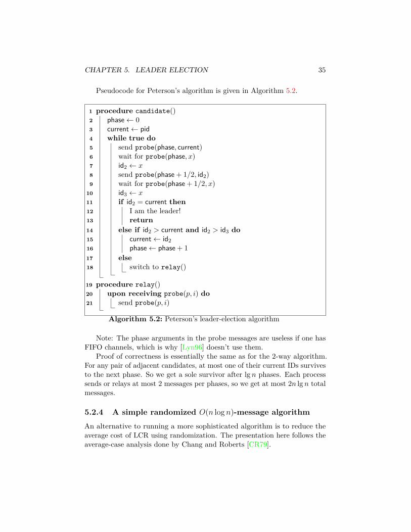
CHAPTER 5. LEADER ELECTION 35

Pseudocode for Peterson’s algorithm is given in Algorithm 5.2.

1 procedure candidate()2 phase← 03 current← pid4 while true do5 send probe(phase, current)6 wait for probe(phase, x)7 id2 ← x8 send probe(phase + 1/2, id2)9 wait for probe(phase + 1/2, x)

10 id3 ← x11 if id2 = current then12 I am the leader!13 return14 else if id2 > current and id2 > id3 do15 current← id216 phase← phase + 117 else18 switch to relay()

19 procedure relay()20 upon receiving probe(p, i) do21 send probe(p, i)

Algorithm 5.2: Peterson’s leader-election algorithm

Note: The phase arguments in the probe messages are useless if one hasFIFO channels, which is why [Lyn96] doesn’t use them.

Proof of correctness is essentially the same as for the 2-way algorithm.For any pair of adjacent candidates, at most one of their current IDs survivesto the next phase. So we get a sole survivor after lgn phases. Each processsends or relays at most 2 messages per phases, so we get at most 2n lgn totalmessages.

5.2.4 A simple randomized O(n log n)-message algorithm

An alternative to running a more sophisticated algorithm is to reduce theaverage cost of LCR using randomization. The presentation here follows theaverage-case analysis done by Chang and Roberts [CR79].

CHAPTER 5. LEADER ELECTION 36

Run LCR where each id is constructed by prepending a long randombit-string to the real id. This gives uniqueness (since the real id’s act astie-breakers) and something very close to a random permutation on theconstructed id’s. When we have unique random id’s, a simple argumentshows that the i-th largest id only propagates an expected n/i hops, givinga total of O(nHn) = O(n logn) hops.4 Unique random id’s occur with highprobability provided the range of the random sequence is n2.

The downside of this algorithm compared to Peterson’s is that knowledgeof n is required to pick random id’s from a large enough range. It also hashigher bit complexity, since Peterson’s algorithm is sending only IDs (in theFIFO-channel version) without any random padding. An possible upside isthat if the range of random ids is large enough, we can run it without anyinitial ids at all, as long as we are willing to accept a small probability ofaccidentally electing two leaders.

5.3 Leader election in general networksFor general networks, a simple approach is to have each node initiate abreadth-first-search and convergecast, with nodes refusing to participate inthe protocol for any initiator with a lower id. It follows that only the nodewith the maximum id can finish its protocol; this node becomes the leader.If messages from parallel broadcasts are combined, it’s possible to keep themessage complexity of this algorithm down to O(DE).

More sophisticated algorithms reduce the message complexity by coalesc-ing local neighborhoods similar to what happens in the Hirschberg-Sinclairand Peterson algorithms. A noteworthy example is an O(n logn) message-complexity algorithm of Afek and Gafni [AG91], who also show an Ω(n logn)lower bound on message complexity for any synchronous algorithm in acomplete network.

5.4 Lower boundsHere we present two classic Ω(logn) lower bounds on message complexityfor leader election in the ring. The first, due to Burns [Bur80], assumesthat the system is asynchronous and that the algorithm is uniform: itdoes not depend on the size of the ring. The second, due to Frederickson

4Alternatively, we could consider the average-case complexity of the algorithm whenwe assume all n! orderings of the ids are equally likely; this also gives O(n logn) expectedmessage complexity [CR79].

CHAPTER 5. LEADER ELECTION 37

and Lynch [FL87], allows a synchronous system and relaxes the uniformityassumption, but requires that the algorithm can’t do anything to ids butcopy and compare them.

5.4.1 Lower bound on asynchronous message complexity

Here we describe a lower bound for uniform asynchronous leader election inthe ring. The description here is based on [AW04, §3.3.3]; a slightly differentpresentation can also be found in [Lyn96, §15.1.4]. The original result is dueto Burns [Bur80]. We assume the system is deterministic.

The basic idea is to construct a bad execution in which n processes sendlots of messages recursively, by first constructing two bad (n/2)-processexecutions and pasting them together in a way that generates many extramessages. If the pasting step produces Θ(n) additional messages, we get arecurrence T (n) ≥ 2T (n/2) + Θ(n) for the total message traffic, which hassolution T (n) = Ω(n logn).

We’ll assume that all processes are trying to learn the identity of theprocess with the smallest id. This is a slightly stronger problem that mereleader election, but it can be solved with at most an additional 2n messagesonce we actually elect a leader. So if we get a lower bound of f(n) messageson this problem, we immediately get a lower bound of f(n)− 2n on leaderelection.

To construct the bad execution, we consider “open executions” on ringsof size n where no message is delivered across some edge (these will be partialexecutions, because otherwise the guarantee of eventual delivery kicks in).Because no message is delivered across this edge, the processes can’t tell ifthere is really a single edge there or some enormous unexplored fragment ofa much larger ring. Our induction hypothesis will show that a line of n/2processes can be made to send at least T (n/2) messages in an open execution(before seeing any messages across the open edge); we’ll then show that alinear number of additional messages can be generated by pasting two suchexecutions together end-to-end, while still getting an open execution with nprocesses.

In the base case, we let n = 1. Somebody has to send a message eventually,giving T (2) ≥ 1.

For larger n, suppose that we have two open executions on n/2 processesthat each send at least T (n/2) messages. Break the open edges in bothexecutions and paste the resulting lines together to get a ring of size n;similarly paste the schedules σ1 and σ2 of the two executions together toget a combined schedule σ1σ2 with at least 2T (n/2) messages. Note that in

CHAPTER 5. LEADER ELECTION 38

the combined schedule no messages are passed between the two sides, so theprocesses continue to behave as they did in their separate executions.

Let e and e′ be the edges we used to past together the two rings. Extendσ1σ2 by the longest possible suffix σ3 in which no messages are deliveredacross e and e′. Since σ3 is as long as possible, after σ1σ2σ3, there are nomessages waiting to be delivered across any edge except e and e′ and allprocesses are quiescent—they will send no additional messages until theyreceive one.

We now consider some suffix σ4 such causes the protocol to finish. Whileexecuting σ4, construct two sets of processes S and S′ by the following rules:

1. If a process is not yet in S or S′ and receives a message delivered acrosse, put it in S; similarly if it receives a message delivered across e′, putit in S′.

2. If a process is not yet in S or S′ and receives a message that was sentby a process in S, put it in S; similarly for S′.

triggered by a delivery across eObserve that S ∪ S′ includes every process on the half of the ring with

the larger minimum id, because any such process that doesn’t receive amessage in σ4 doesn’t learn the global minimum. So |S ∪ S′| ≥ n/2 and thusmin(|S|, |S′|) ≥ n/4.

Assume without loss of generality that it is |S| that is at least n/4.Except for the two processes incident to e, every process that is added to Sis added in response to a message sent in σ4. So there are at least n/4− 2such messages. We can also argue that all of these messages are sent inthe subschedule τ of σ4 that contains only messages that do not depend onmessages delivered across e′. It follows that σ1σ2σ3τ is an open executionon n processes with at least 2T (n/2) + n/4 − 2 sent messages. This givesT (n) ≥ 2T (n/2) + n/4− 2 = 2T (n/2) + Ω(n) as claimed.

5.4.2 Lower bound for comparison-based algorithms

Here we give an Ω(n logn) lower bound on messages for synchronous-startcomparison-based algorithms in bidirectional synchronous rings. For fulldetails see [Lyn96, §3.6], [AW04, §3.4.2], or the original JACM paper byFrederickson and Lynch [FL87].

Basic ideas:

• Two fragments i . . . i+k and j . . . j+k of a ring are order-equivalentprovided idi+a > idi+b if and only if idj+a > idj+b for b = 0 . . . k.

CHAPTER 5. LEADER ELECTION 39

• An algorithm is comparison-based if it can’t do anything to IDs butcopy them and test for <. The state of such an algorithm is modeledby some non-ID state together with a big bag of IDs, messages have apile of IDs attached to them, etc. Two states/messages are equivalentunder some mapping of IDs if you can translate the first to the secondby running all IDs through the mapping.An equivalent version uses an explicit equivalence relation betweenprocesses. Let executions of p1 and p2 be similar if both processessend messages in the same direction(s) in the same rounds and bothprocesses declare themselves leader (or not) at the same round. Thenan algorithm is comparison-based based if order-equivalent rings yieldsimilar executions for corresponding processes. This can be turnedinto the explicit-copying-IDs model by replacing the original protocolwith a full-information protocol in which each message is replacedby the ID and a complete history of the sending process (including allmessages it has every received).

• Define an active round as a round in which at least one messageis sent. Claim: Actions of i after k active rounds depends, up to anorder-equivalent mapping of ids, only on the order-equivalence class ofids in i− k . . . i+ k, the k-neighborhood of i. Proof: by induction onk. Suppose i and j have order-equivalent (k − 1)-neighborhoods; thenafter k − 1 active rounds they have equivalent states by the inductionhypothesis. In inactive rounds, i and j both receive no messages andupdate their states in the same way. In active rounds, i and j receiveorder-equivalent messages and update their states in an order-equivalentway.

• If we have an order of ids with a lot of order-equivalent k-neighborhoods,then after k active rounds if one process sends a message, so do a lotof other ones.

Now we just need to build a ring with a lot of order-equivalent neighbor-hoods. For n a power of 2 we can use the bit-reversal ring, e.g., id sequence000, 100, 010, 110, 001, 101, 011, 111 (in binary) when n = 8. Figure 5.1 givesa picture of what this looks like for n = 32.

For n not a power of 2 we look up Frederickson and Lynch [FL87] orAttiya et al. [ASW88]. In either case we get Ω(n/k) order-equivalent membersof each equivalence class after k active rounds, giving Ω(n/k) messages peractive round, which sums to Ω(n logn).

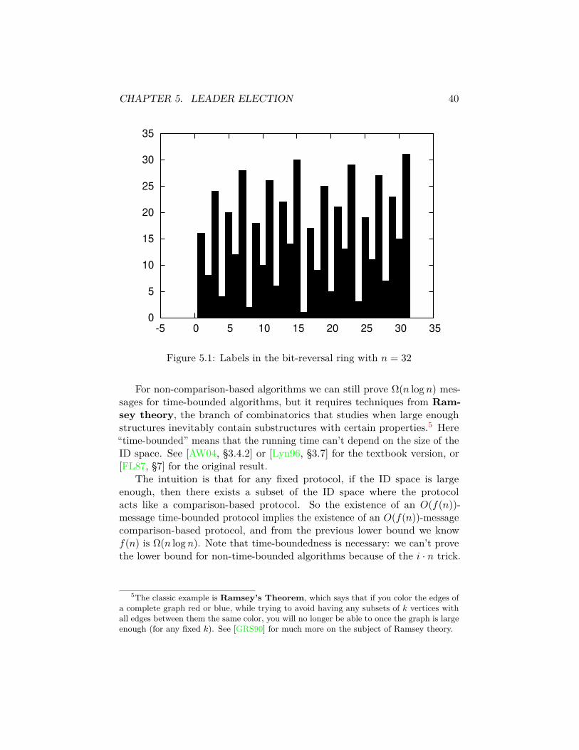
CHAPTER 5. LEADER ELECTION 40

0

5

10

15

20

25

30

35

-5 0 5 10 15 20 25 30 35

Figure 5.1: Labels in the bit-reversal ring with n = 32

For non-comparison-based algorithms we can still prove Ω(n logn) mes-sages for time-bounded algorithms, but it requires techniques from Ram-sey theory, the branch of combinatorics that studies when large enoughstructures inevitably contain substructures with certain properties.5 Here“time-bounded” means that the running time can’t depend on the size of theID space. See [AW04, §3.4.2] or [Lyn96, §3.7] for the textbook version, or[FL87, §7] for the original result.

The intuition is that for any fixed protocol, if the ID space is largeenough, then there exists a subset of the ID space where the protocolacts like a comparison-based protocol. So the existence of an O(f(n))-message time-bounded protocol implies the existence of an O(f(n))-messagecomparison-based protocol, and from the previous lower bound we knowf(n) is Ω(n logn). Note that time-boundedness is necessary: we can’t provethe lower bound for non-time-bounded algorithms because of the i · n trick.

5The classic example is Ramsey’s Theorem, which says that if you color the edges ofa complete graph red or blue, while trying to avoid having any subsets of k vertices withall edges between them the same color, you will no longer be able to once the graph is largeenough (for any fixed k). See [GRS90] for much more on the subject of Ramsey theory.

Chapter 6

Logical clocks

Logical clocks assign a timestamp to all events in an asynchronous message-passing system that simulates real time, thereby allowing timing-based algo-rithms to run despite asynchrony. In general, they don’t have anything todo with clock synchronization or wall-clock time; instead, they provide nu-merical values that increase over time and are consistent with the observablebehavior of the system. This means that local events on a single processhave increasing times, and messages are never delivered before they are sent,when time is measured using the logical clock.

6.1 Causal orderingThe underlying notion of a logical clock is causal ordering, a partial orderon events that describes when one event e provably occurs before some otherevent e′.

For the purpose of defining casual ordering and logical clocks, we willassume that a schedule consists of send events and receive events, whichcorrespond to some process sending a single message or receiving a singlemessage, respectively.

Given two schedules S and S′, call S and S′ similar if S|p = S′|p for allprocesses p; in other words, S and S′ are similar if they are indistinguishableby all participants. We can define a causal ordering on the events of someschedule S implicitly by considering all schedules S′ similar to S, and declarethat e < e′ if e precedes e′ in all such S. But it is usually more useful tomake this ordering explicit.

Following [AW04, §6.1.1] (and ultimately [Lam78]), define the happens-before relation ⇒

Son a schedule S to consist of:

41

CHAPTER 6. LOGICAL CLOCKS 42

1. All pairs (e, e′) where e precedes e′ in S and e and e′ are events of thesame process.

2. All pairs (e, e′) where e is a send event and e′ is the receive event forthe same message.

3. All pairs (e, e′) where there exists a third event e′′ such that e ⇒Se′′

and e′′ ⇒Se′. (In other words, we take the transitive closure of the

relation defined by the previous two cases.)

It is not terribly hard to show that this gives a partial order; the mainobservation is that if e⇒

Se′, then e precedes e′ in S. So ⇒

Sis a subset of the

total order <S given by the order of events in S.A causal shuffle S′ of a schedule S is a permutation of S that is

consistent with the happens-before relation on S; that is, if e happens-beforee′ in S, then e precedes e′ in S′. The importance of the happens-beforerelation follows from the following lemma, which says that the causal shufflesof S are precisely the schedules S′ that are similar to S.

Lemma 6.1.1. Let S′ be a permutation of the events in S. Then thefollowing two statements are equivalent:

1. S′ is a causal shuffle of S.

2. S′ is the schedule of an execution fragment of a message-passing systemwith S|p = S′|p for all S′.

Proof. (1⇒ 2). We need to show both similarity and that S′ corresponds tosome execution fragment. We’ll show similarity first. Pick some p; then everyevent at p in S also occurs in S′, and they must occur in the same order bythe first case of the definition of the happens-before relation. This gets ushalfway to showing S′ is the schedule of some execution fragment, since itsays that any events initiated by p are consistent with p’s programming. Toget the rest of the way, observe that any other events are receive events. Foreach receive event e′ in S, there must be some matching send event e also inS; thus e and e′ are both in S′ and occur in the right order by the secondcase of the definition of happens-before.

(2 ⇒ 1). First observe that since every event e in S′ occurs at someprocess p, if S′|p = S|p for all p, then there is a one-to-one correspondencebetween events in S′ and S, and thus S′ is a permutation of S. Now we needto show that S′ is consistent with ⇒

S. Let e⇒

Se′. There are three cases.

CHAPTER 6. LOGICAL CLOCKS 43

1. e and e′ are events of the same process p and e <S e′. But then e <S′ e′because S|p = S′|p.

2. e is a send event and e′ is the corresponding receive event. Thene <S′ e

′ because S′ is the schedule of an execution fragment.

3. e⇒Se′ by transitivity. Then each step in the chain connecting e to e′

uses one of the previous cases, and e <S′ e′ by transitivity of <S′ .

There are two main applications for causal shuffles:

1. We can prove upper bounds by using a causal shuffle to turn somearbitrary S into a nice S′, and argue that the niceness of S′ meansthat S at least looks nice to the processes. An example of this can befound in Lemma 7.1.1.

2. We can prove lower bounds by using a causal shuffle to turn somespecific S into a nasty S′, and argue that the existence of S′ tells usthat there exist bad schedules for some particular problem. An exampleof this can be found in §7.4.2. This works particularly well because ⇒

Sincludes enough information to determine the latest possible time ofany event in either S or S′, so rearranging schedules like this doesn’tchange the worst-case time.

In both cases, we are using the fact that if I tell you ⇒S, then you know

everything there is to know about the order of events in S that you candeduce from reports from each process together with the fact that messagesdon’t travel back in time.

In the case that we want to use this information inside an algorithm, werun into the issue that ⇒

Sis a pretty big relation (Θ(|S|2) bits with a naive

encoding), and seems to require global knowledge of <S to compute. So wecan ask if there is some simpler, easily computable description that worksalmost as well. This is where logical clocks come in.

6.2 ImplementationsThe basic idea of a logical clock is to compute a timestamp for each event,so that comparing timestamps gives information about ⇒

S. Note that these

timestamps need not be totally ordered. In general, we will have a relation

CHAPTER 6. LOGICAL CLOCKS 44

<L between timestamps such that e⇒Se′ implies e <L e′, but it may be that

there are some pairs of events that are ordered by the logical clock despitebeing incomparable in the happens-before relation.

Examples of logical clocks that use small timestamps but add extraordering are Lamport clocks [Lam78], discussed in §6.2.1; and Neiger-Toueg-Welch clocks [NT87, Wel87], discussed in §6.2.2. These both assign integertimestamps to events and may order events that are not causally related.The main difference between them is that Lamport clocks do not alter theunderlying execution, but may allow arbitrarily large jumps in the logicalclock values; while Neiger-Toueg-Welch clocks guarantee small increments atthe cost of possibly delaying parts of the system.1

More informative are vector clocks [Fid91, Mat93], discussed in §6.2.3.These use n-dimensional vectors of integers to capture ⇒

Sexactly, at the cost

of much higher overhead.

6.2.1 Lamport clock

Lamport’s logical clock [Lam78] runs on top of any other message-passingprotocol, adding additional state at each process and additional content tothe messages (which is invisible to the underlying protocol). Every processmaintains a local variable clock. When a process sends a message or executesan internal step, it sets clock ← clock + 1 and assigns the resulting valueas the clock value of the event. If it sends a message, it piggybacks theresulting clock value on the message. When a process receives a message withtimestamp t, it sets clock ← max(clock, t) + 1; the resulting clock value istaken as the time of receipt of the message. (To make life easier, we assumemessages are received one at a time.)

Theorem 6.2.1. If we order all events by clock value, we get an executionof the underlying protocol that is locally indistinguishable from the originalexecution.

Proof. Let e <L e′ if e has a lower clock value than e′. If e and e′ are twoevents of the same process, then e <L e′. If e and e′ are send and receiveevents of the same message, then again e <L e′. So for any events e, e′, ife⇒Se′, then e <L e′. Now apply Lemma 6.1.1.

1This makes them similar to synchronizers, which we will discuss in Chapter 7.

CHAPTER 6. LOGICAL CLOCKS 45

6.2.2 Neiger-Toueg-Welch clock

Lamport’s clock has the advantage of requiring no changes in the behaviorof the underlying protocol, but has the disadvantage that clocks are entirelyunder the control of the logical-clock protocol and may as a result makehuge jumps when a message is received. If this is unacceptable—perhaps theprotocol needs to do some unskippable maintenance task every 1000 clockticks—then an alternative approach due to Neiger and Toueg [NT87] andWelch [Wel87] can be used.

Method: Each process maintains its own variable clock, which it in-crements whenever it feels like it. To break ties, the process extends theclock value to 〈clock, id, eventCount〉 where eventCount is a count of send andreceive events (and possibly local computation steps). As in Lamport’s clock,each message in the underlying protocol is timestamped with the currentextended clock value. Because the protocol can’t change the clock values onits own, when a message is received with a timestamp later than the currentextended clock value, its delivery is delayed until clock exceeds the messagetimestamp, at which point the receive event is assigned the extended clockvalue of the time of delivery.

Theorem 6.2.2. If we order all events by clock value, we get an executionof the underlying protocol that is locally indistinguishable from the originalexecution.

Proof. Again, we have that (a) all events at the same process occur inincreasing order (since the event count rises even if the clock value doesn’t,and we assume that the clock value doesn’t drop) and (b) all receive eventsoccur later than the corresponding send event (since we force them to). SoLemma 6.1.1 applies.

The advantage of the Neiger-Toueg-Welch clock is that it doesn’t imposeany assumptions on the clock values, so it is possible to make clock be areal-time clock at each process and nonetheless have a causally-consistentordering of timestamps even if the local clocks are not perfectly synchronized.If some process’s clock is too far off, it will have trouble getting its messagesdelivered quickly (if its clock is ahead) or receiving messages (if its clock isbehind)—the net effect is to add a round-trip delay to that process equalto the difference between its clock and the clock of its correspondent. Butthe protocol works well when the processes’ clocks are closely synchronized,which is a reasonable assumption in many systems thanks to the Network

CHAPTER 6. LOGICAL CLOCKS 46

Time Protocol, cheap GPS receivers, and clock synchronization mechanismsbuilt into most cellular phone networks.2

6.2.3 Vector clocks

Logical clocks give a superset of the happens-before relation: if e⇒Se′, then

e <L e′ (or conversely, if e 6<L e′, then it is not the case that e⇒

Se′). This

is good enough for most applications, but what if we want to compute ⇒S

exactly?Here we can use a vector clock, invented independently by Fidge [Fid91]

and Mattern [Mat93]. Instead of a single clock value, each event is stampedwith a vector of values, one for each process. When a process executes alocal event or a send event, it increments only its own component xp of thevector. When it receives a message, it increments xp and sets each xq to themax of its previous value and the value of xq piggybacked on the message.We define VC(e) ≤ VC(e′), where VC(e) is the value of the vector clock for e,if VC(e)i ≤ VC(e′)i for all i.

Theorem 6.2.3. Fix a schedule S; then for any e, e′, V C(e) < V C(e′) ifand only if e⇒

Se′.

Proof. The if part follows immediately from the update rules for the vectorclock. For the only if part, suppose e does not happen-before e′. Then e ande′ are events of distinct processes p and p′. For VC(e) < VC(e′) to hold, wemust have VC(e)p < VC(e′)p; but this can occur only if the value of VC(e)pis propagated to p′ by some sequence of messages starting at p and endingat p′ at or before e′ occurs. In this case we have e⇒

Se′.

6.3 Consistent snapshotsA consistent snapshot of a message-passing computation is a descriptionof the states of the processes (and possibly messages in transit, but wecan reduce this down to just states by keeping logs of messages sent andreceived) that gives the global configuration at some instant of a schedulethat is a consistent reordering of the real schedule (a consistent cut inthe terminology of [AW04, §6.1.2]. Without shutting down the protocol

2As I write this, my computer reports that its clock is an estimated 289 microsecondsoff from the timeserver it is synchronized to, which is less than a tenth of the round-tripdelay to machines on the same local-area network and a tiny fraction of the round-tripdelay to machines elsewhere, including the timeserver machine.

CHAPTER 6. LOGICAL CLOCKS 47

before taking a snapshot this is the about the best we can hope for in amessage-passing system.

Logical clocks can be used to obtain consistent snapshots: pick somelogical clock time and have each process record its state at this time (i.e.,immediately after its last step before the time or immediately before its firststep after the time). We have already argued that the logical clock gives aconsistent reordering of the original schedule, so the set of values recorded isjust the configuration at the end of an appropriate prefix of this reordering.In other words, it’s a consistent snapshot.

If we aren’t building logical clocks anyway, there is a simpler consistentsnapshot algorithm due to Chandy and Lamport [CL85]. Here some centralinitiator broadcasts a snap message, and each process records its state andimmediately forwards the snap message to all neighbors when it first receivesa snap message. To show that the resulting configuration is a configurationof some consistent reordering, observe that (with FIFO channels) no processreceives a message before receiving snap that was sent after the sender sentsnap: thus causality is not violated by lining up all the pre-snap operationsbefore all the post-snap ones.3

The full Chandy-Lamport algorithm adds a second marker message that isused to sweep messages in transit out of the communications channels, whichavoids the need to keep logs if we want to reconstruct what messages are intransit (this can also be done with the logical clock version). The idea is thatwhen a process records its state after receiving the snap message, it issuesa marker message on each outgoing channel. For incoming channels, theprocess all records all messages received between the snapshot and receivinga marker message on that channel (or nothing if it receives marker beforereceiving snap). A process only reports its value when it has received amarker on each channel. The marker and snap messages can also be combinedif the broadcast algorithm for snap resends it on all channels anyway, and afurther optimization is often to piggyback both on messages of the underlyingprotocol if the underlying protocol is chatty enough.

Note that Chandy-Lamport is equivalent to the logical-time snapshotusing Lamport clocks, if the snap message is treated as a message with avery large timestamp. For Neiger-Toueg-Welch clocks, we get an algorithmwhere processes spontaneously decide to take snapshots (since Neiger-Toueg-Welch clocks aren’t under the control of the snapshot algorithm) and delay

3If FIFO channels are not available, they can be simulated in the absence of failures byadding a sequence number to each outgoing message on a given channel, and processingmessages at the recipient only when all previous messages have been processed.

CHAPTER 6. LOGICAL CLOCKS 48

post-snapshot messages until the local snapshot has been taken. This can beimplemented as in Chandy-Lamport by separating pre-snapshot messagesfrom post-snapshot messages with a marker message, and essentially turnsinto Chandy-Lamport if we insist that a process advance its clock to thesnapshot time when it receives a marker.

6.3.1 Property testing

Consistent snapshots are in principle useful for debugging (since one cangather a consistent state of the system without being able to talk to everyprocess simultaneously), and in practice are mostly used for detecting stableproperties of the system. Here a stable property is some predicate onglobal configurations that remains true in any successor to a configurationin which it is true, or (bending the notion of properties a bit) functionson configurations whose values don’t change as the protocol runs. Typicalexamples are quiescence and its evil twin, deadlock. More exotic examplesinclude total money supply in a banking system that cannot create or destroymoney, or the fact that every process has cast an irrevocable vote in favorof some proposal or advanced its Neiger-Toueg-Welch-style clock past somethreshold.

The reason we can test such properties using consistent snapshot isthat when the snapshot terminates with value C in some configuration C ′,even though C may never have occurred during the actual execution of theprotocol, there is an execution which leads from C to C ′. So if P holds inC, stability means that it holds in C ′.

Naturally, if P doesn’t hold in C, we can’t say much. So in this case were-run the snapshot protocol and hope we win next time. If P eventuallyholds, we will eventually start the snapshot protocol after it holds and obtaina configuration (which again may not correspond to any global configurationthat actually occurs) in which P holds.

Chapter 7

Synchronizers

Synchronizers simulate an execution of a failure-free synchronous systemin a failure-free asynchronous system. See [AW04, Chapter 11] or [Lyn96,Chapter 16] for a detailed (and rigorous) presentation.

7.1 DefinitionsFormally, a synchronizer sits between the underlying network and the pro-cesses and does one of two things:

• A global synchronizer guarantees that no process receives a messagefrom round r until all processes have sent their messages for round r.

• A local synchronizer guarantees that no process receives a mes-sage from round r until all of that process’s neighbors have sent theirmessages for round r.

In both cases, the synchronizer packages all the incoming round r mes-sages m for a single process together and delivers them as a single actionrecv(p,m, r). Similarly, a process is required to hand over all of its outgoinground-r messages to the synchronizer as a single action send(p,m, r)—thisprevents a process from changing its mind and sending an extra round-rmessage or two. It is easy to see that the global synchronizer producesexecutions that are effectively indistinguishable from synchronous executions,assuming that a synchronous execution is allowed to have some variability inexactly when within a given round each process does its thing. The localsynchronizer only guarantees an execution that is locally indistinguishablefrom an execution of the global synchronizer: an individual process can’t

49

CHAPTER 7. SYNCHRONIZERS 50

tell the difference, but comparing actions at different (especially widely sepa-rated) processes may reveal some process finishing round r + 1 while othersare still stuck in round r or earlier. Whether this is good enough depends onwhat you want: it’s bad for coordinating simultaneous missile launches, butmay be just fine for adapting a synchronous message-passing algorithm (aswith distributed breadth-first search as described in §4.3) to an asynchronoussystem, if we only care about the final states of the processes and not whenprecisely those states are reached.

Formally, the relation between global and local synchronization is de-scribed by the following lemma:

Lemma 7.1.1. For any schedule S of a locally synchronous execution, thereis a schedule S′ of a globally synchronous execution such that S|p = S′|p forall processes p.

Proof. Essentially, we use the same happens-before relation as in Chapter 6,and the fact that if a schedule S′ is a causal shuffle of another schedule S(i.e., a permutation of T that preserves causality), then S′|p = S|p for all p(Lemma 6.1.1).

Given a schedule S, consider a schedule S′ in which the events are orderedfirst by increasing round and then by putting all sends before receives. Thisordering is consistent with ⇒

S, so it’s a causal shuffle of S and S′|p = S|p.

But it is globally synchronized, because no round r operation ever happensbefore a round (r − 1) operation.

7.2 ImplementationsHere we describe several implementations of synchronizers. All of them giveat least local synchrony. One of them, the beta synchronizer (§7.2.2), alsogives global synchrony.

The names were chosen by their inventor, Baruch Awerbuch [Awe85].The main difference between them is the mechanism used to determine whenround-r messages have been delivered.

In the alpha synchronizer, every node sends a message to every neigh-bor in every round (possibly a dummy message if the underlying protocoldoesn’t send a message); this allows the receiver to detect when it’s gottenall its round-r messages (because it expects to get a message from everyneighbor) but may produce huge blow-ups in message complexity in a densegraph.

CHAPTER 7. SYNCHRONIZERS 51

In the beta synchronizer, messages are acknowledged by their receivers(doubling the message complexity), so the senders can detect when all oftheir messages are delivered. But now we need a centralized mechanism tocollect this information from the senders and distribute it to the receivers,since any particular receiver doesn’t know which potential senders to wait for.This blows up time complexity, as we essentially end up building a globalsynchronizer with a central leader.

The gamma synchronizer combines the two approaches at differentlevels to obtain a trade-off between messages and time that depends on thestructure of the graph and how the protocol is organized.

Details of each synchronizer are given below.

7.2.1 The alpha synchronizer

The alpha synchronizer uses local information to construct a local synchro-nizer. In round r, the synchronizer at p sends p’s message (tagged with theround number) to each neighbor p′ or noMsg(r) if it has no messages. Whenit collects a message or noMsg from each neighbor for round r, it deliversall the messages. It’s easy to see that this satisfies the local synchronizationspecification.

This produces no change in time but may drastically increase messagecomplexity because of all the extra noMsg messages flying around. For asynchronous protocol that runs in T rounds with M messages, the sameprotocol running with the alpha synchronizer will still run in T time units,but the message complexity will go up to T · |E| messages, or worse if theoriginal algorithm doesn’t detect termination.

7.2.2 The beta synchronizer

The beta synchronizer centralizes detection of message delivery using a rooteddirected spanning tree (previously constructed). When p′ receives a round-rmessage from p, it responds with ack(r). When p collects an ack for all themessages it sent plus an OK from all of its children, it sends OK to its parent.When the root has all the ack and OK messages it is expecting, it broadcastsgo. Receiving go makes p deliver the queued round-r messages.

This works because in order for the root to issue go, every round-rmessage has to have gotten an acknowledgment, which means that all round-r messages are waiting in the receivers’ buffers to be delivered. For the betasynchronizer, message complexity for one round increases slightly from M to

CHAPTER 7. SYNCHRONIZERS 52

2M + 2(n− 1), but time complexity goes up by a factor proportional to thedepth of the tree.

7.2.3 The gamma synchronizer

The gamma synchronizer combines the alpha and beta synchronizers to tryto get low blowups on both time complexity and message complexity. Theessential idea is to cover the graph with a spanning forest and run betawithin each tree and alpha between trees. Specifically:

• Every message in the underlying protocol gets acked (including mes-sages that pass between trees).

• When a process has collected all of its outstanding round-r acks, itsends OK up its tree.

• When the root of a tree gets all acks and OK, it sends ready to theroots of all adjacent trees (and itself). Two trees are adjacent if any oftheir members are adjacent.

• When the root collects ready from itself and all adjacent roots, itbroadcasts go through its own tree.

As in the alpha synchronizer, we can show that no root issues go unless itand all its neighbors issue ready, which happens only after both all nodes inthe root’s tree and all their neighbors (some of whom might be in adjacenttrees) have received acks for all messages. This means that when a nodereceives go it can safely deliver its bucket of messages.

Message complexity is comparable to the beta synchronizer assumingthere aren’t too many adjacent trees: 2M messages for sends and acks,plus O(n) messages for in-tree communication, plus O(Eroots) messages forroot-to-root communication. Time complexity per synchronous round isproportional to the depth of the trees: this includes both the time for in-treecommunication, and the time for root-to-root communication, which mightneed to be routed through leaves.

In a particularly nice graph, the gamma synchronizer can give costscomparable to the costs of the original synchronous algorithm. An examplein [Lyn96] is a ring of k-cliques, where we build a tree in each clique and getO(1) time blowup and O(n) added messages. This is compared to O(n/k)time blowup for the beta synchronizer and O(k) message blowup (or worse)for the alpha synchronizer. Other graphs may favor tuning the size of the

CHAPTER 7. SYNCHRONIZERS 53

trees in the forest toward the alpha or beta ends of the spectrum, e.g., ifthe whole graph is a clique (and we didn’t worry about contention issues),we might as well just use beta and get O(1) time blowup and O(n) addedmessages.

7.3 ApplicationsSee [AW04, §11.3.2] or [Lyn96, §16.5]. The one we have seen is distributedbreadth-first search, where the two asynchronous algorithms we described inChapter 4 were essentially the synchronous algorithms with the beta andalpha synchronizers embedded in them. But what synchronizers give us ingeneral is the ability to forget about problems resulting from asynchronyprovided we can assume no failures (which may be a very strong assumption)and are willing to accept a bit of overhead.

7.4 Limitations of synchronizersHere we show some lower bounds on synchronizers, justifying our previousclaim that failures are trouble and showing that global synchronizers arenecessarily slow in a high-diameter network.

7.4.1 Impossibility with crash failures

These synchronizers all fail badly if some process crashes. In the α synchro-nizer, the system slowly shuts down as a wave of waiting propagates outfrom the dead process. In the β synchronizer, the root never gives the greenlight for the next round. The γ synchronizer, true to its hybrid nature, failsin a way that is a hybrid of these two disasters.

This is unavoidable in the basic asynchronous model, although we don’thave all the results we need to prove this yet. The idea is that if we are in asynchronous system with crash failures, it’s possible to solve agreement, theproblem of getting all the processes to agree on a bit (see Chapter 9). Butit’s not possible to solve this problem in an asynchronous system with evenone crash failure (see Chapter 11). Since a synchronous-with-crash-failureagreement protocol on top of a fault-tolerant synchronizer would give asolution to an unsolvable problem, the element of this stack that we don’tknow an algorithm for must be the one we can’t do. Hence there are nofault-tolerant synchronizers.

CHAPTER 7. SYNCHRONIZERS 54

We’ll see more examples of this trick of showing that a particular simula-tion is impossible because it would allow us to violate impossibility resultslater, especially when we start looking at the strength of shared-memoryobjects in Chapter 18.

7.4.2 Unavoidable slowdown with global synchronization

The session problem [AFL83] gives a lower bound on the speed of a globalsynchronizer, or more generally on any protocol that tries to approximatesynchrony in a certain sense. Recall that in a global synchronizer, our goal isto produce a simulation that looks synchronous from the outside; that is, thatlooks synchronous to an observer that can see the entire schedule. In contrast,a local synchronizer produces a simulation that looks synchronous fromthe inside—the resulting execution is indistinguishable from a synchronousexecution to any of the processes, but an outside observer can see thatdifferent processes execute different rounds at different times. The globalsynchronizer we’ve seen takes more time than a local synchronizer; the sessionproblem shows that this is necessary.

In our description, we will mostly follow [AW04, §6.2.2].A solution to the session problem is an asynchronous protocol in which

each process repeatedly executes some special action. Our goal is toguarantee that these special actions group into s sessions, where a sessionis an interval of time in which every process executes at least one specialaction. We also want the protocol to terminate: this means that in everyexecution, every process executes a finite number of special actions.

A synchronous system can solve this problem trivially in s rounds: eachprocess executes one special action per round. For an asynchronous system, alower bound of Attiya and Mavronicolas [AM94] (based on an earlier boundof Arjomandi, Fischer, and Lynch [AFL83], who defined the problem ina slightly different communication model), shows that if the diameter ofthe network is D, there is no solution to the s-session problem that takes(s− 1)D time or less in the worst case. The argument is based on reorderingevents in any such execution to produce fewer than s sessions, using thehappens-before relation described in Chapter 6.

We now give an outline of the proof that this is expensive. (See [AW04,§6.2.2] for the real proof.)

Fix some algorithm A for solving the s-session problem, and suppose thatits worst-case time complexity is (s−1)D or less. Consider some synchronousexecution of A (that is, one where the adversary scheduler happens to arrangethe schedule to be synchronous) that takes (s− 1)D rounds or less. Divide

CHAPTER 7. SYNCHRONIZERS 55

this execution into two segments: an initial segment β that includes allrounds with special actions, and a suffix δ that includes any extra roundswhere the algorithm is still floundering around. We will mostly ignore δ, butwe have to leave it in to allow for the possibility that whatever is happeningthere is important for the algorithm to work (say, to detect termination).

We now want to perform a causal shuffle on β that leaves it with onlys− 1 sessions. Because causal shuffles don’t affect time complexity, this willgive us a new bad execution β′δ that has only s− 1 sessions despite taking(s− 1)D time.

The first step is to chop β into at most s− 1 segments β1, β2, . . . of atmost D rounds each. Because a message sent in round i is not delivered untilround i+ 1, if we have a chain of k messages, each of which triggers the next,then if the first message is sent in round i, the last message is not delivereduntil round i+ k. If the chain has length D, its events (including the initialsend and the final delivery) span D + 1 rounds i, i + 1, . . . , i + D. In thiscase the initial send and final delivery are necessarily in different segmentsβi and βi+1.

Now pick processes p0 and p1 at distance D from each other. Then anychain of messages starting at p0 within some segment reaches p1 after theend of the segment. It follows that for any events e0 of p0 and e1 of p1 inthe same segment βi, e0 6⇒

βδe1. So there exists a causal shuffle of βi that

puts all events of p0 after all events of p1.1 By a symmetrical argument, wecan similarly put all events of p1 after all events of p0. In both cases theresulting schedule is indistinguishable by all processes from the original.

So now we apply these shuffles to each of the segments βi in alternatingorder: p0 goes first in the even-numbered segments and p1 goes first in theodd-numbered segments, yielding a sequence of shuffled segments β′i. Thishas the effect of putting the p0 events together, as in this example with(s− 1) = 4:

βδ|(p0, p1) = β1β2β3β4δ|(p0, p1)= β′1β

′2β′3β′4δ|(p0, p1)

= (p1p0)(p0p1)(p1p0)(p0p1)δ= p1(p0p0)(p1p1)(p0p0)p1δ

(here each p0, p1 stands in for a sequence of events of each process).1Proof: Because e0 6⇒

βδe1, we can add e1 < e0 for all events e1 and e0 in βi and still

have a partial order consistent with ⇒βδ. Now apply topological sort to get the shuffle.

CHAPTER 7. SYNCHRONIZERS 56

Now let’s count sessions. We can’t end a session until we reach a pointwhere both processes have taken at least one step since the end of the lastsession. If we mark with a slash the earliest places where this can happen,we get a picture like this:

p1p0/p0p1/p1p0/p0p1/p1δ.

We have at most s− 1 sessions! This concludes the proof.

Chapter 8

Coordinated attack

(See also [Lyn96, §5.1].)The Two Generals problem was the first widely-known distributed con-

sensus problem, described in 1978 by Jim Gray [Gra78, §5.8.3.3.1], althoughthe same problem previously appeared under a different name [AEH75].

The setup of the problem is that we have two generals on opposite sidesof an enemy army, who must choose whether to attack the army or retreat.If only one general attacks, his troops will be slaughtered. So the generalsneed to reach agreement on their strategy.

To complicate matters, the generals can only communicate by sendingmessages by (unreliable) carrier pigeon. We also suppose that at some pointeach general must make an irrevocable decision to attack or retreat. Theinteresting property of the problem is that if carrier pigeons can becomelost, there is no protocol that guarantees agreement in all cases unless theoutcome is predetermined (e.g., the generals always attack no matter whathappens). The essential idea of the proof is that any protocol that doesguarantee agreement can be shortened by deleting the last message; iteratingthis process eventually leaves a protocol with no messages.

Adding more generals turns this into the coordinated attack problem,a variant of consensus; but it doesn’t make things any easier.

8.1 Formal descriptionTo formalize this intuition, suppose that we have n ≥ 2 generals in asynchronous system with unreliable channels—the set of messages receivedin round i+ 1 is always a subset of the set sent in round i, but it may bea proper subset (even the empty set). Each general starts with an input 0

57

CHAPTER 8. COORDINATED ATTACK 58

(retreat) or 1 (attack) and must output 0 or 1 after some bounded numberof rounds. The requirements for the protocol are that, in all executions:

Agreement All processes output the same decision (0 or 1).

Validity If all processes have the same input x, and no messages are lost,all processes produce output x. (If processes start with different inputsor one or more messages are lost, processes can output 0 or 1 as longas they all agree.)

Termination All processes terminate in a bounded number of rounds.1

Sadly, there is not protocol that satisfies all three conditions. We showthis in the next section.

8.2 Impossibility proofTo show coordinated attack is impossible,2 we use an indistinguishabilityproof .

The basic idea of an indistinguishability proof is this:

• Execution A is indistinguishable from execution B for some processp if p sees the same things (messages or operation results) in bothexecutions.

• If A is indistinguishable from B for p, then because p can’t tell whichof these two possible worlds it is in, it returns the same output in both.

So far, pretty dull. But now let’s consider a chain of hypotheticalexecutions A = A0A1 . . . Ak = B, where each Ai is indistinguishable fromAi+1 for some process pi. Suppose also that we are trying to solve anagreement task, where every process must output the same value. Then sincepi outputs the same value in Ai and Ai+1, every process outputs the same

1Bounded means that there is a fixed upper bound on the length of any execution.We could also demand merely that all processes terminate in a finite number of rounds.In general, finite is a weaker requirement than bounded, but if the number of possibleoutcomes at each step is finite (as they are in this case), they’re equivalent. The reasonis that if we build a tree of all configurations, each configuration has only finitely manysuccessors, and the length of each path is finite, then König’s lemma (see http://en.wikipedia.org/wiki/Konig’s_lemma) says that there are only finitely many paths. So wecan take the length of the longest of these paths as our fixed bound. [BG97, Lemma 3.1]

2Without making additional assumptions, always a caveat when discussing impossibility.

CHAPTER 8. COORDINATED ATTACK 59

value in Ai and Ai+1. By induction on k, every process outputs the samevalue in A and B, even though A and B may be very different executions.

This gives us a tool for proving impossibility results for agreement: showthat there is a path of indistinguishable executions between two executionsthat are supposed to produce different output. Another way to picture this:consider a graph whose nodes are all possible executions with an edge betweenany two indistinguishable executions; then the set of output-0 executionscan’t be adjacent to the set of output-1 executions. If we prove the graph isconnected, we prove the output is the same for all executions.

For coordinated attack, we will show that no protocol satisfies all ofagreement, validity, and termination using an indistinguishability argument.The key idea is to construct a path between the all-0-input and all-1-inputexecutions with no message loss via intermediate executions that are indis-tinguishable to at least one process.

Let’s start with A = A0 being an execution in which all inputs are 1 andall messages are delivered. We’ll build executions A1, A2, etc., by pruningmessages. Consider Ai and let m be some message that is delivered inthe last round in which any message is delivered. Construct Ai+1 by notdelivering m. Observe that while Ai is distinguishable from Ai+1 by therecipient of m, on the assumption that n ≥ 2 there is some other processthat can’t tell whether m was delivered or not (the recipient can’t let thatother process know, because no subsequent message it sends are deliveredin either execution). Continue until we reach an execution Ak in which allinputs are 1 and no messages are sent. Next, let Ak+1 through Ak+n beobtained by changing one input at a time from 1 to 0; each such executionis indistinguishable from its predecessor by any process whose input didn’tchange. Finally, construct Ak+n through Ak+n+k′ by adding back messagesin the reverse process used for A0 through Ak; note that this might notresult in exactly k new messages, because the number of messages mightdepend on the inputs. This gets us to an execution Ak+n+k′ in which allprocesses have input 0 and no messages are lost. If agreement holds, thenthe indistinguishability of adjacent executions to some process means thatthe common output in A0 is the same as in Ak+n+k′ . But validity requiresthat A0 outputs 1 and Ak+n+k′ outputs 0: so either agreement or validity isviolated in some execution.

CHAPTER 8. COORDINATED ATTACK 60

8.3 Randomized coordinated attackSo we now know that we can’t solve the coordinated attack problem. Butmaybe we want to solve it anyway. The solution is to change the problem.

Randomized coordinated attack is like standard coordinated attack,but with less coordination. Specifically, we’ll allow the processes to flipcoins to decide what to do, and assume that the communication pattern(which messages get delivered in each round) is fixed and independent ofthe coin-flips. This corresponds to assuming an oblivious adversary thatcan’t see what is going on at all or perhaps a content-oblivious adversarythat can only see where messages are being sent but not the contents of themessages. We’ll also relax the agreement property to only hold with somehigh probability:

Randomized agreement For any adversary A, the probability that someprocess decides 0 and some other process decides 1 given A is at mostε.

Validity and termination are as before.

8.3.1 An algorithm

Here’s an algorithm that gives ε = 1/r. (See [Lyn96, §5.2.2] for detailsor [VL92] for the original version.) A simplifying assumption is that networkis complete, although a strongly-connected network with r greater than orequal to the diameter also works.

• First part: tracking information levels

– Each process tracks its “information level,” initially 0. The stateof a process consists of a vector of (input, information-level) pairsfor all processes in the system. Initially this is (my-input, 0) foritself and (⊥,−1) for everybody else.

– Every process sends its entire state to every other process in everyround.

– Upon receiving a message m, process i stores any inputs carried inm and, for each process j, sets leveli[j] to max(leveli[j], levelm[j]).It then sets its own information level to minj(leveli[j]) + 1.

• Second part: deciding the output

– Process 1 chooses a random key value uniformly in the range [1, r].

CHAPTER 8. COORDINATED ATTACK 61

– This key is distributed along with leveli[1], so that every processwith leveli[1] ≥ 0 knows the key.

– A process decides 1 at round r if and only if it knows the key,its information level is greater than or equal to the key, and allinputs are 1.

8.3.2 Why it works

Termination Immediate from the algorithm.

Validity • If all inputs are 0, no process sees all 1 inputs (technicallyrequires an invariant that processes’ non-null views are consistentwith the inputs, but that’s not hard to prove.)

• If all inputs are 1 and no messages are lost, then the informationlevel of each process after k rounds is k (prove by induction) andall processes learn the key and all inputs (immediate from firstround). So all processes decide 1.

Randomized Agreement • First prove a lemma: Define levelti[k] tobe the value of leveli[k] after t rounds. Then for all i, j, k, t, (1)leveli[j]t ≤ levelj [j]t−1 and (2)

∣∣leveli[k]t − levelj [k]t∣∣ ≤ 1. As

always, the proof is by induction on rounds. Part (1) is easy andboring so we’ll skip it. For part (2), we have:– After 0 rounds, level0i [k] = level0j [k] = −1 if neither i nor j

equals k; if one of them is k, we have level0k[k] = 0, which isstill close enough.

– After t rounds, consider levelti[k] − levelt−1i [k] and similarly

leveltj [k]−levelt−1j [k]. It’s not hard to show that each can jump

by at most 1. If both deltas are +1 or both are 0, there’sno change in the difference in views and we win from theinduction hypothesis. So the interesting case is when leveli[k]stays the same and levelj [k] increases or vice versa.

– There are two ways for levelj [k] to increase:∗ If j 6= k, then j received a message from some j′ with

levelt−1j′ [k] > levelt−1

j [k]. From the induction hypothesis,levelt−1

j′ [k] ≤ levelt−1i [k] + 1 = levelti[k]. So we are happy.

∗ If j = k, then j has leveltj [j] = 1 + mink 6=j leveltj [k] ≤1 + leveltj [i] ≤ 1 + levelti[i]. Again we are happy.

CHAPTER 8. COORDINATED ATTACK 62

• Note that in the preceding, the key value didn’t figure in; soeverybody’s level at round r is independent of the key.

• So now we have that levelri [i] is in `, `+ 1, where ` is some fixedvalue uncorrelated with the key. The only way to get some processto decide 1 while others decide 0 is if `+ 1 ≥ key but ` < key. (If` = 0, a process at this level doesn’t know key, but it can stillreason that 0 < key since key is in [1, r].) This can only occur ifkey = `+ 1, which occurs with probability at most 1/r since keywas chosen uniformly.

8.3.3 Almost-matching lower bound

The bound on the probability of disagreement in the previous algorithm isalmost tight. Varghese and Lynch [VL92] show that no synchronous algorithmcan get a probability of disagreement less than 1

r+1 , using a stronger validitycondition that requires that the processes output 0 if any input is 0. This isa natural assumption for database commit, where we don’t want to commitif any process wants to abort. We restate their result below:

Theorem 8.3.1. For any synchronous algorithm for randomized coordinatedattack that runs in r rounds that satisfies the additional condition that allnon-faulty processes decide 0 if any input is 0, Pr[disagreement] ≥ 1/(r + 1).

Proof. Let ε be the bound on the probability of disagreement. Define levelti[k]as in the previous algorithm (whatever the real algorithm is doing). We’llshow Pr[i decides 1] ≤ ε · (levelri [i] + 1), by induction on levelri [i].

• If levelri [i] = 0, the real execution is indistinguishable (to i) from anexecution in which some other process j starts with 0 and receives nomessages at all. In that execution, j must decide 0 or risk violatingthe strong validity assumption. So i decides 1 with probability at mostε (from the disagreement bound).

• If levelri [i] = k > 0, the real execution is indistinguishable (to i) froman execution in which some other process j only reaches level k − 1and thereafter receives no messages. From the induction hypothesis,Pr[j decides 1] ≤ εk in that pruned execution, and so Pr[i decides 1] ≤ε(k + 1) in the pruned execution. But by indistinguishability, we alsohave Pr[i decides 1] ≤ ε(k + 1) in the original execution.

Now observe that in the all-1 input execution with no messages lost,levelri [i] = r and Pr[i decides 1] = 1 (by validity). So 1 ≤ ε(r + 1), whichimplies ε ≥ 1/(r + 1).

Chapter 9

Synchronous agreement

Here we’ll consider synchronous agreement algorithm with stopping failures,where a process stops dead at some point, sending and receiving no furthermessages. We’ll also consider Byzantine failures, where a process deviatesfrom its programming by sending arbitrary messages, but mostly just to seehow crash-failure algorithms hold up; for algorithms designed specifically fora Byzantine model, see Chapter 10.

If the model has communication failures instead, we have the coordinatedattack problem from Chapter 8.

9.1 Problem definitionWe use the usual synchronous model with n processes with binary inputs andbinary outputs. Up to f processes may fail at some point; when a processfails, one or one or more of its outgoing messages are lost in the round offailure and all outgoing messages are lost thereafter.

There are two variants on the problem, depending on whether we wanta useful algorithm (and so want strong conditions to make our algorithmmore useful) or a lower bound (and so want weak conditions to make ourlower bound more general). For algorithms, we will ask for these conditionsto hold:

Agreement All non-faulty processes decide the same value.

Validity If all processes start with the same input, all non-faulty processesdecide it.

Termination All non-faulty processes eventually decide.

63

CHAPTER 9. SYNCHRONOUS AGREEMENT 64

For lower bounds, we’ll replace validity with non-triviality (often calledvalidity in the literature):

Non-triviality There exist failure-free executions A and B that producedifferent outputs.

Non-triviality follows from validity but doesn’t imply validity; for example,a non-trivial algorithm might have the property that if all non-faulty processesstart with the same input, they all decide something else.

In §9.2, we’ll show that a simple algorithm gives agreement, termination,and validity with f failures using f + 1 rounds. We’ll then show in §9.3 thatnon-triviality, agreement, and termination imply that f + 1 rounds is thebest possible. In Chapter 10, we’ll show that the agreement is still possiblein f + 1 rounds even if faulty processes can send arbitrary messages insteadof just crashing, but only if the number of faulty processes is strictly lessthan n/3.

9.2 Solution using floodingThe flooding algorithm, due to Dolev and Strong [DS83] gives a straightfor-ward solution to synchronous agreement for the crash failure case. It runs inf + 1 rounds assuming f crash failures. (This algorithm is also described inmore detail in [AW04, §5.1.3] or [Lyn96, §6.2.1].)

Each process keeps a set of (process, input) pairs, initially just (myId,myInput).At round r, I broadcast my set to everybody and take the union of my setand all sets I receive. At round f + 1, I decide on f(S), where f is somefixed function from sets of process-input pairs to outputs that picks someinput in S: for example, f might take the input with the smallest process-idattached to it, take the max of all known input values, or take the majorityof all known input values.

Lemma 9.2.1. After f + 1 rounds, all non-faulty processes have the sameset.

Proof. Let Sri be the set stored by process i after r rounds. What we’ll reallyshow is that if there are no failures in round k, then Sri = Srj = Sk+1

i for alli, j, and r > k. To show this, observe that no faults in round k means thatall processes that are still alive at the start of round k send their messageto all other processes. Let L be the set of live processes in round k. At theend of round k, for i in L we have Sk+1

i =⋃j∈L S

kj = S. Now we’ll consider

some round r = k + 1 +m and show by induction on m that Sk+mi = S; we

CHAPTER 9. SYNCHRONOUS AGREEMENT 65

already did m = 0, so for larger m notice that all messages are equal to Sand so Sk+1+m

i is the union of a whole bunch of S’s. So in particular wehave Sf+1

i = S (since some failure-free round occurred in the preceding f + 1rounds) and everybody decides the same value f(S).

Flooding depends on being able to trust second-hand descriptions ofvalues; it may be that process 1 fails in round 0 so that only process 2 learnsits input. If process 2 can suddenly tell 3 (but nobody else) about the inputin round f + 1—or worse, tell a different value to 3 and 4—then we mayget disagreement. This remains true even if Byzantine processes can’t fakeinputs (e.g., because an input value is really a triple (i, v, signature(v)) usingan unforgeable digital signature)—the reason is that a Byzantine processcould horde some input (i, v, signature(v)) until the very last round and thendeliver it to only some of the non-faulty processes.

9.3 Lower bound on roundsHere we show that synchronous agreement requires at least f + 1 roundsif f processes can fail. This proof is modeled on the one in [Lyn96, §6.7]and works backwards from the final state; for a proof of the same resultthat works in the opposite direction, see [AW04, §5.1.4]. The original result(stated for Byzantine failures) is due to Dolev and Strong [DS83], based ona more complicated proof due to Fischer and Lynch [FL82]; see the chapternotes for Chapter 5 of [AW04] for more discussion of the history.

Note that unlike the algorithms in the preceding and following sections,which provide validity, the lower bound applies even if we only demandnon-triviality.

Like the similar proof for coordinated attack (§8.2), the proof uses anindistinguishability argument. But we have to construct a more complicatedchain of intermediate executions.

A crash failure at process i means that (a) in some round r, some orall of the messages sent by i are not delivered, and (b) in subsequent rounds,no messages sent by i are delivered. The intuition is that i keels over deadin the middle of generating its outgoing messages for a round. Otherwise ibehaves perfectly correctly. A process that crashes at some point during anexecution is called faulty

We will show that if up to f processes can crash, and there are at leastf + 2 processes,1 then at least f + 1 rounds are needed (in some execution)

1With only f + 1 processes, we can solve agreement in f rounds using flooding. The

CHAPTER 9. SYNCHRONOUS AGREEMENT 66

for any algorithm that satisfies agreement, termination, and non-triviality.In particular, we will show that if all executions run in f or fewer rounds,then the indistinguishability graph is connected; this implies non-trivialitydoesn’t hold, because (as in §8.2), two adjacent states must decide the samevalue because of the agreement property.2

Now for the proof. To simplify the argument, let’s assume that allexecutions terminate in exactly f rounds (we can always have processes sendpointless chitchat to pad out short executions) and that every processes sendsa message to every other process in every round where it has not crashed(more pointless chitchat). Formally, this means we have a sequence of rounds0, 1, 2, . . . , f − 1 where each process sends a message to every other process(assuming no crashes), and a final round f where all processes decide on avalue (without sending any additional messages).

We now want to take any two executions A and B and show that bothproduce the same output. To do this, we’ll transform A’s inputs into B’sinputs one process at a time, crashing processes to hide the changes. Theproblem is that just crashing the process whose input changed might changethe decision value—so we have to crash later witnesses carefully to maintainindistinguishability all the way across the chain.

Let’s say that a process p crashes fully in round r if it crashes in roundr and no round-r messages from p are delivered. The communicationpattern of an execution describes which messages are delivered betweenprocesses without considering their contents—in particular, it tells us whichprocesses crash and what other processes they manage to talk to in the roundin which they crash.

With these definitions, we can state and prove a rather complicatedinduction hypothesis:

Lemma 9.3.1. For any f -round protocol with n ≥ f+2 processes permittingup to f crash failures; any process p; and any execution A in which atmost one process crashes per round in rounds 0 . . . r − 1, p crashes fully inround r + 1, and no other processes crash; there is a sequence of executionsA = A0A1 . . . Ak such that each Ai is indistinguishable from Ai+1 by some

idea is that either (a) at most f − 1 processes crash, in which case the flooding algorithmguarantees agreement; or (b) exactly f processes crash, in which case the one remainingnon-faulty process agrees with itself. So f + 2 processes are needed for the lower boundto work, and we should be suspicious of any lower bound proof that does not use thisassumption.

2The same argument works with even a weaker version of non-triviality that omits therequirement that A and B are failure-free, but we’ll keep things simple.

CHAPTER 9. SYNCHRONOUS AGREEMENT 67

process, each Ai has at most one crash per round, and the communicationpattern in Ak is identical to A except that p crashes fully in round r.

Proof. By induction on f − r. If r = f , we just crash p in round r andnobody else notices. For r < f , first crash p in round r instead of r + 1, butdeliver all of its round-r messages anyway (this is needed to make space forsome other process to crash in round r + 1). Then choose some message msent by p in round r, and let p′ be the recipient of m. We will show that wecan produce a chain of indistinguishable executions between any executionin which m is delivered and the corresponding execution in which it is not.

If r = f − 1, this is easy; only p′ knows whether m has been delivered,and since n ≥ f + 2, there exists another non-faulty p′′ that can’t distinguishbetween these two executions, since p′ sends no messages in round f or later.If r < f − 1, we have to make sure p′ doesn’t tell anybody about the missingmessage.

By the induction hypothesis, there is a sequence of executions startingwith A and ending with p′ crashing fully in round r + 1, such that eachexecution is indistinguishable from its predecessor. Now construct thesequence

A→ (A with p′ crashing fully in r + 1)→ (A with p′ crashing fully in r + 1 and m lost)→ (A with m lost and p′ not crashing).

The first and last step apply the induction hypothesis; the middle one yieldsindistinguishable executions since only p′ can tell the difference between marriving or not and its lips are sealed.

We’ve shown that we can remove one message through a sequence ofexecutions where each pair of adjacent executions is indistinguishable tosome process. Now paste together n− 1 such sequences (one per message)to prove the lemma.

The rest of the proof: Crash some process fully in round 0 and thenchange its input. Repeat until all inputs are changed.

9.4 VariantsSo far we have described binary consensus, since all inputs are 0 or 1. Wecan also allow larger input sets. With crash failures, this allows a strongervalidity condition: the output must be equal to some non-faulty process’s

CHAPTER 9. SYNCHRONOUS AGREEMENT 68

input. It’s not hard to see that Dolev-Strong (§9.2) gives this strongercondition.

Chapter 10

Byzantine agreement

Like synchronous agreement (as in Chapter 9) except that we replace crashfailures with Byzantine failures, where a faulty process can ignore itsprogramming and send any messages it likes. Since we are operating undera universal quantifier, this includes the case where the Byzantine processesappear to be colluding with each other under the control of a centralizedadversary.

10.1 Lower boundsWe’ll start by looking at lower bounds.

10.1.1 Minimum number of rounds

We’ve already seen an f+1 lower bound on rounds for crash failures (see §9.3).This lower bound applies a fortiori to Byzantine failures, since Byzantinefailures can simulate crash failures.

10.1.2 Minimum number of processes

We can also show that we need n > 3f processes. For n = 3 and f = 1 theintuition is that Byzantine B can play non-faulty A and C off against eachother, telling A that C is Byzantine and C that A is Byzantine. Since A istelling C the same thing about B that B is saying about A, C can’t tell thedifference and doesn’t know who to believe. Unfortunately, this tragic soapopera is not a real proof, since we haven’t actually shown that B can sayexactly the right thing to keep A and C from guessing that B is evil.

69

CHAPTER 10. BYZANTINE AGREEMENT 70

A0 B0

C

A0 B0

C0

A1B1

C1

Figure 10.1: Three-process vs. six-process execution in Byzantine agreementlower bound. Processes A0 and B0 in right-hand execution receive samemessages as in left-hand three-process execution with Byzantine C simulationC0 through C1. So validity forces them to decide 0. A similar argumentusing Byzantine A shows the same for C0.

The real proof:1 Consider an artificial execution where (non-Byzantine)A, B, and C are duplicated and then placed in a ring A0B0C0A1B1C1, wherethe digits indicate inputs. We’ll still keep the same code for n = 3 on A0, B0,etc., but when A0 tries to send a message to what it thinks of as just C we’llsend it to C1 while messages from B0 will instead go to C0. For any adjacentpair of processes (e.g. A0 and B0), the behavior of the rest of the ring couldbe simulated by a single Byzantine process (e.g. C), so each process in the6-process ring behaves just as it does in some 3-process execution with 1Byzantine process. It follows that all of the processes terminate and decidein the unholy 6-process Frankenexecution2 the same value that they would inthe corresponding 3-process Byzantine execution. So what do they decide?

Given two processes with the same input, say, A0 and B0, the giantexecution is indistinguishable from an A0B0C execution where C is Byzantine(see Figure 10.1. Validity says A0 and B0 must both decide 0. Since thisworks for any pair of processes with the same input, we have each processdeciding its input. But now consider the execution of C0A1B, where B isByzantine. In the big execution, we just proved that C0 decides 0 and A1decides 1, but since the C0A1B execution is indistinguishable from the bigexecution to C0 and A1, they do the same thing here and violate agreement.

This shows that with n = 3 and f = 1, we can’t win. We can generalizethis to n = 3f . Suppose that there were an algorithm that solved Byzantineagreement with n = 3f processes. Group the processes into groups of size f ,and let each of the n = 3 processes simulate one group, with everybody in

1The presentation here is based on [AW04, §5.2.3]. The original impossibility resultis due to Pease, Shostak, and Lamport [PSL80]. This particular proof is due to Fischer,Lynch, and Merritt [FLM86].

2Not a real word.

CHAPTER 10. BYZANTINE AGREEMENT 71

A0

B0

C

D0

A0

B0

D0

C0

A1B1

C1

D1

Figure 10.2: Four-process vs. eight-process execution in Byzantine agreementconnectivity lower bound. Because Byzantine C can simulate C0, D1, B1, A1,and C1, good processes A0, B0 and D0 must all decide 0 or risk violatingvalidity.

the group getting the same input, which can only make things easier. Thenwe get a protocol for n = 3 and f = 1, an impossibility.

10.1.3 Minimum connectivity

So far, we’ve been assuming a complete communication graph. If the graph isnot complete, we may not be able to tolerate as many failures. In particular,we need the connectivity of the graph (minimum number of nodes that mustbe removed to split it into two components) to be at least 2f +1. See [Lyn96,§6.5] for the full proof. The essential idea is that if we have an arbitrarygraph with a vertex cut of size k < 2f + 1, we can simulate it on a 4-processgraph where A is connected to B and C (but not D), B and C are connectedto each other, and D is connected only to B and C. Here B and C eachsimulate half the processes in the size-k cut, A simulates all the processeson one side of the cut and D all the processes on the other side. We thenconstruct an 8-process artificial execution with two non-faulty copies of eachof A, B, C, and D and argue that if one of B or C can be Byzantine thenthe 8-process execution is indistinguishable to the remaining processes froma normal 4-process execution. (See Figure 10.1.)

An argument similar to the n > 3f proof then shows we violate one ofvalidity or agreement: if we replacing C0, C1, and all the nodes on one side ofthe C0 +C1 cut with a single Byzantine C, we force the remaining non-faultynodes to decide their inputs or violate validity. But then doing the same

CHAPTER 10. BYZANTINE AGREEMENT 72

thing with B0 and B1 yields an execution that violates agreement.Conversely, if we have connectivity 2f+1, then the processes can simulate

a general graph by sending each other messages along 2f + 1 predeterminedvertex-disjoint paths and taking the majority value as the correct message.Since the f Byzantine processes can only corrupt one path each (assumingthe non-faulty processes are careful about who they forward messages from),we get at least f+1 good copies overwhelming the f bad copies. This reducesthe problem on a general graph with sufficiently high connectivity to theproblem on a complete graph, allowing Byzantine agreement to be solved ifthe other lower bounds are met.

10.1.4 Weak Byzantine agreement

(Here we are following [Lyn96, §6.6]. The original result is due to Lam-port [Lam83].)

Weak Byzantine agreement is like regular Byzantine agreement, butvalidity is only required to hold if there are no faulty processes at all. Ifthere is a single faulty process, the non-faulty processes can output any valueregardless of their inputs (as long as they agree on it). Sadly, this weakeningdoesn’t improve things much: even weak Byzantine agreement can be solvedonly if n ≥ 3f + 1.

Proof: As in the strong Byzantine agreement case, we’ll construct a many-process Frankenexecution to figure out a strategy for a single Byzantineprocess in a 3-process execution. The difference is that now the number ofprocesses in our synthetic execution is much larger, since we want to buildan execution where at least some of our test subjects think they are in a non-Byzantine environment. The trick is to build a very big, highly-symmetricring so that at least some of the processes are so far away from the fewpoints of asymmetry that might clue them in to their odd condition that theprotocol terminates before they notice.

Fix some protocol that allegedly solves weak Byzantine agreement, andlet r be the number of rounds for the protocol. Construct a ring of 6r pro-cesses A01B01C01A02B02C02 . . . A0rB0rC0rA10B10C10 . . . A1rB1rC1r, whereeach Xij runs the code for process X in the 3-process protocol with in-put i. For each adjacent pair of processes, there is a 3-process Byzantineexecution which is indistinguishable from the 6r-process execution for thatpair: since agreement holds in all Byzantine executions, each adjacent pairdecides the same value in the big execution and so either everybody decides0 or everybody decides 1 in the big execution.

Now we’ll show that means that validity is violated in some no-failures

CHAPTER 10. BYZANTINE AGREEMENT 73

3-process execution. We’ll extract this execution by looking at the executionof processes A0,r/2B0,r/2C0,r/2. The argument is that up to round r, anyinput-0 process that is at least r steps in the ring away from the nearest1-input process acts like the corresponding process in the all-0 no-failures3-process execution. Since A0,r/2 is 3r/2 > r hops away from A1r andsimilarly for C0,r/2, our 3 stooges all decide 0 by validity. But now repeatthe same argument for A1,r/2B1,r/2C1,r/2 and get 3 new stooges that alldecide 1. This means that somewhere in between we have two adjacentprocesses where one decides 0 and one decides 1, violating agreement in thecorresponding 3-process execution where the rest of the ring is replaced by asingle Byzantine process. This concludes the proof.

This result is a little surprising: we might expect that weak Byzantineagreement could be solved by allowing a process to return a default value ifit notices anything that might hint at a fault somewhere. But this wouldallow a Byzantine process to create disagreement revealing its bad behaviorto just one other process in the very last round of an execution otherwiseheaded for agreement on the non-default value. The chosen victim decides thedefault value, but since it’s the last round, nobody else finds out. Even if thealgorithm is doing something more sophisticated, examining the 6r-processexecution will tell the Byzantine process exactly when and how to startacting badly.

10.2 Upper boundsHere we describe two upper bounds for Byzantine agreement, one of whichgets an optimal number of rounds at the cost of many large messages, andthe other of which gets smaller messages at the cost of more rounds. (Weare following §§5.2.4–5.2.5 of [AW04] in choosing these algorithms.) Neitherof these algorithms is state-of-the-art, but they demonstrate some of theissues in solving Byzantine agreement without the sometimes-complicatedoptimizations needed to get all the parameters of the algorithm down simul-taneously.

10.2.1 Exponential information gathering gets n = 3f + 1The idea of exponential information gathering is that each process willdo a lot of gossiping, but now its state is no longer just a flat set of inputs,but a tree describing who it heard what from. We build this tree out of pairsof the form (path, input) where path is a sequence of intermediaries with norepetitions and input is some input. A process’s state at each round is just a

CHAPTER 10. BYZANTINE AGREEMENT 74

set of such pairs. At the end of f + 1 rounds of communication (necessarybecause of the lower bound for crash failures), each non-faulty processattempts to untangle the complex web of hearsay and second-hand lies tocompute the same decision value as the other processes. This technique wasused by Pease, Shostak, and Lamport [PSL80] to show that their impossibilityresult is tight: there exists an algorithm for Byzantine agreement that runsin f + 1 synchronous rounds and guarantees agreement and validity as longas n ≥ 3f + 1.

1 S ← 〈〈〉 , input〉2 for round← 0 . . . f do3 Send 〈xi, v〉 | 〈x, v〉 ∈ S ∧ |x| = round ∧ i 6∈ x to all processes4 upon receiving S′ from j do

// Filter out obviously bogus tuples5 if ∀ 〈xj′, v〉 ∈ S′ : |x| = round ∧ j′ = j then6 S ← S ∪ S′

// Compute decision value7 for each path w of length f + 1 with no repeats do8 if 〈w, v〉 ∈ S for some v then9 Let val′(w, i) = v

10 else11 Let val′(w, i) = 0

12 for each path w of length f or less with no repeats do13 Let val′(w, i) = majorityj 6∈w val(wj, i)14 Decide val′(〈〉 , i)Algorithm 10.1: Exponential information gathering. Code for pro-cess i.

The algorithm is given in Algorithm 10.1. The communication phase isjust gossiping, where each process starts with its only its input and forwardsany values it hears about along with their provenance to all of the otherprocesses. At the end of this phase, each process has a set of pairs of theform (path, value) where path spans all sequences of 0 to f + 1 distinct idsand value is the input value forwarded along that path.

We write val(w, i) for the value stored in i’s list at the end of the protocolthat is associated with path w. Because we can’t trust these val(w, i) valuesto be an accurate description of any process’s input if there is a Byzantineprocess in w, each process computes for itself replacement values val′(w, i)

CHAPTER 10. BYZANTINE AGREEMENT 75

that use majority voting to try to get a more trustworthy picture of theoriginal inputs.

Formally, we think of the set of paths as a tree where w is the parent ofwj for each path w and each id j not in w. To apply EIG in the Byzantinemodel, ill-formed messages received from j are treated as missing messages,but otherwise the data-collecting part of EIG proceeds as in the crash failuremodel. However, we compute the decision value from the last-round valuesrecursively as follows. First replace any missing pair involving a path w with|w| = f + 1 with (w, 0). Then for each path w, define val′(w, i) to be themajority value among val′(wj, i) for all j, or val(w, i) if |w| = f + 1. Finally,have process i decide val′(〈〉 , i), which it can compute locally from its ownstored values val(w, i).

Each val′ is a reconstruction of older values from later ones. As we moveup the tree from wj to w we are moving backwards in time, until in theend we get the decision value val′(〈〉, i) as a majority of reconstructed inputsval′(j, i). One way to think about this is that I don’t trust j to give me theright value for wj—even when w = 〈〉 and j is claiming to report its owninput—so instead I take a majority of values of wj that j allegedly reportedto other people. But since I don’t trust those other people either, I use thesame process recursively to construct those reports.

10.2.1.1 Proof of correctness

This is just a sketch of the proof from [Lyn96, §6.3.2]; essentially the sameargument appears in [AW04, §5.2.4].

We start with a basic observation that good processes send and recordvalues correctly:

Lemma 10.2.1. If i, j, and k are all non-faulty then for all w, val(wk, i) =val(wk, j) = val(w, k).

Proof. Trivial: k announces the same value val(w, k) to both i and j.

More involved is this lemma, which says that when we reconstruct avalue for a trustworthy process at some level, we get the same value that itsent us. In particular this will be used to show that the reconstructed inputsval′(j, i) are all equal to the real inputs for good processes.

Lemma 10.2.2. If j is non-faulty then val′(wj, i) = val(w, j) for all non-faulty i and all w.

CHAPTER 10. BYZANTINE AGREEMENT 76

Proof. By induction on f + 1 − |wj|. If |wj| = f + 1, then val′(wj, i) =val(wj, i) = val(w, j). If |wj| < f + 1, then val(wj, k) = val(w, j) for all non-faulty k. It follows that val(wjk, i) = val(w, j) for all non-faulty i and k (thatdo not appear in w). The bad guys report at most f bad values val(wj, k′),but the good guys report at least n− f − |wj| good values val(wj, k). Sincen ≥ 3f + 1 and |wj| ≤ f , we have n − f − |wj| ≥ 3f + 1 − f − f ≥ f + 1good values, which are a majority.

We call a node w common if val′(w, i) = val′(w, j) for all non-faulty i, j.Lemma 10.2.2 implies that wk is common if k is non-faulty. We can alsoshow that any node whose children are all common is also common, whetheror not the last process in its label is faulty.Lemma 10.2.3. Let wk be common for all k. Then w is common.Proof. Recall that, for |w| < f + 1, val′(w, i) is the majority value amongall val′(wk, i). If all wk are common, then val′(wk, i) = val′(wk, j) for allnon-faulty i and j, so i and j compute the same majority values and getval′(w, i) = val′(w, j).

We can now prove the full result.Theorem 10.2.4. Exponential information gathering using f + 1 roundsin a synchronous Byzantine system with at most f faulty processes satisfiesvalidity and agreement, provided n ≥ 3f + 1.Proof. Validity: Immediate application of Lemmas 10.2.1 and 10.2.2 whenw = 〈〉. We have val′(j, i) = val(j, i) = val(〈〉, j) for all non-faulty j and i,which means that a majority of the val′(j, i) values equal the common inputand thus so does val′(〈〉, i).

Agreement: Observe that every path has a common node on it, since apath travels through f +1 nodes and one of them is good. If we then supposethat the root is not common: by Lemma 10.2.3, it must have a not-commonchild, that node must have a not-common child, etc. But this constructsa path from the root to a leaf with no not-common nodes, which we justproved can’t happen.

10.2.2 Phase king gets constant-size messages

The following algorithm, based on work of Berman, Garay, and Perry [BGP89],achieves Byzantine agreement in 2(f+1) rounds using constant-size messages,provided n ≥ 4f + 1. The description here is drawn from [AW04, §5.2.5].The original Berman-Garay-Perry paper gives somewhat better bounds, butthe algorithm and its analysis are more complicated.

CHAPTER 10. BYZANTINE AGREEMENT 77

10.2.2.1 The algorithm

The basic idea of the algorithm is that we avoid the recursive majority votingof EIG by running a vote in each of f + 1 phases through a phase king,some process chosen in advance to run the phase. Since the number of phasesexceeds the number of faults, we eventually get a non-faulty phase king.The algorithm is structured so that one non-faulty phase king is enoughto generate agreement and subsequent faulty phase kings can’t undo theagreement.

Pseudocode appears in Algorithm 10.2. Each processes i maintains anarray prefi[j], where j ranges over all process ids. There are also utilityvalues majority, kingMajority and multiplicity for each process that are usedto keep track of what it hears from the other processes. Initially, prefi[i] isjust i’s input and prefi[j] = 0 for j 6= i.

1 prefi[i] = input2 for j 6= i do prefi[j] = 03 for k ← 1 to f + 1 do

// First round of phase k4 send prefi[i] to all processes (including myself)5 prefi[j]← vj , where vj is the value received from process j6 majority← majority value in prefi7 multiplicity← number of times majority appears in prefi

// Second round of phase k8 if i = k then

// I am the phase king9 send majority to all processes

10 if received m from phase king then11 kingMajority← m12 else13 kingMajority← 014 if multiplicity > n/2 + f then15 prefi[i] = majority16 else17 prefi[i] = kingMajority

18 return prefi[i]Algorithm 10.2: Byzantine agreement: phase king

The idea of the algorithm is that in each phase, everybody announces their

CHAPTER 10. BYZANTINE AGREEMENT 78

current preference (initially the inputs). If the majority of these preferencesis large enough (e.g., all inputs are the same), everybody adopts the majoritypreference. Otherwise everybody adopts the preference of the phase king.The majority rule means that once the processes agree, they continue toagree despite bad phase kings. The phase king rule allows a good phase kingto end disagreement. By choosing a different king in each phase, after f + 1phases, some king must be good. This intuitive description is justified below.

10.2.2.2 Proof of correctness

Termination is immediate from the algorithm.For validity, suppose all inputs are v. We’ll show that all non-faulty i

have prefi[i] = v after every phase. In the first round of each phase, processi receives at least n− f messages containing v; since n ≥ 4f + 1, we haven− f ≥ 3f + 1 and n/2 + f ≤ (4f + 1)/2 + f = 3f + 1/2, and thus thesen− f messages exceed the n/2 + f threshold for adopting them as the newpreference. So all non-faulty processes ignore the phase king and stick withv, eventually deciding v after round 2(f + 1).

For agreement, we’ll ignore all phases up to the first phase with a non-faulty phase king. Let k be the first such phase, and assume that the prefvalues are set arbitrarily at the start of this phase. We want to argue thatat the end of the phase, all non-faulty processes have the same preference.There are two ways that a process can set its new preference in the secondround of the phase:

1. The process i observes a majority of more than n/2 +f identical valuesv and ignores the phase king. Of these values, more than n/2 of themwere sent by non-faulty processes. So the phase king also receives thesevalues (even if the faulty processes change their stories) and choosesv as its majority value. Similarly, if any other process j observes amajority of n/2 + f identical values, the two > n/2 non-faulty parts ofthe majorities overlap, and so j also chooses v.

2. The process i takes its value from the phase king. We’ve already shownthat i then agrees with any j that sees a big majority; but since thephase king is non-faulty, process i will agree with any process j thatalso takes its new preference from the phase king.

This shows that after any phase with a non-faulty king, all processesagree. The proof that the non-faulty processes continue to agree is the sameas for validity.

CHAPTER 10. BYZANTINE AGREEMENT 79

10.2.2.3 Performance of phase king

It’s not hard to see that this algorithm sends exactly (f+1)(n2 +n) messagesof 1 bit each (assuming 1-bit inputs). The cost is doubling the minimumnumber of rounds and reducing the tolerance for Byzantine processes. Asmentioned earlier, a variant of phase-king with 3-round phases gets optimalfault-tolerance with 3(f + 1) rounds (but 2-bit messages). Still better isa rather complicated descendant of the EIG algorithm due to Garay andMoses [GM98], which gets f + 1 rounds with n ≥ 3f + 1 while still havingpolynomial message traffic.

Chapter 11

Impossibility ofasynchronous agreement

There’s an easy argument that says that you can’t do most things in anasynchronous message-passing system with n/2 crash failures: partition theprocesses into two subsets S and T of size n/2 each, and allow no messagesbetween the two sides of the partition for some long period of time. Sincethe processes in each side can’t distinguish between the other side beingslow and being dead, eventually each has to take action on their own. Formany problems, we can show that this leads to a bad configuration. Forexample, for agreement, we can supply each side of the partition with adifferent common input value, forcing disagreement because of validity. Wecan then satisfy the fairness condition that says all messages are eventuallydelivered by delivering the delayed messages across the partition, but it’stoo late for the protocol.

The Fischer-Lynch-Paterson (FLP) result [FLP85] says something muchstronger: you can’t do agreement in an asynchronous message-passing systemif even one crash failure is allowed.1 After its initial publication, it was quicklygeneralized to other models including asynchronous shared memory [LAA87],and indeed the presentation of the result in [Lyn96, §12.2] is given for shared-memory first, with the original result appearing in [Lyn96, §17.2.3] as acorollary of the ability of message passing to simulate shared memory. Inthese notes, I’ll present the original result; the dependence on the model issurprisingly limited, and so most of the proof is the same for both sharedmemory (even strong versions of shared memory that support operations

1Unless you augment the basic model in some way, say by adding randomization(Chapter 23) or failure detectors (Chapter 13).

80

CHAPTER 11. IMPOSSIBILITY OF ASYNCHRONOUS AGREEMENT81

like atomic snapshots2) and message passing.Section 5.3 of [AW04] gives a very different version of the proof, where

it is shown first for two processes in shared memory, then generalized to nprocesses in shared memory by adapting the classic Borowsky-Gafni simu-lation [BG93] to show that two processes with one failure can simulate nprocesses with one failure. This is worth looking at (it’s an excellent exampleof the power of simulation arguments, and BG simulation is useful in manyother contexts) but we will stick with the original argument, which is simpler.We will look at this again when we consider BG simulation in Chapter 27.

11.1 AgreementUsual rules: agreement (all non-faulty processes decide the same value),termination (all non-faulty processes eventually decide some value), valid-ity (for each possible decision value, there an execution in which that valueis chosen). Validity can be tinkered with without affecting the proof much.

To keep things simple, we assume the only two decision values are 0 and1.

11.2 FailuresA failure is an internal action after which all send operations are disabled.The adversary is allowed one failure per execution. Effectively, this meansthat any group of n− 1 processes must eventually decide without waitingfor the n-th, because it might have failed.

11.3 StepsThe FLP paper uses a notion of steps that is slightly different from thesend and receive actions of the asynchronous message-passing model we’vebeen using. Essentially a step consists of receiving zero or more messagesfollowed by doing a finite number of sends. To fit it into the model we’ve beenusing, we’ll define a step as either a pair (p,m), where p receives messagem and performs zero or more sends in response, or (p,⊥), where p receivesnothing and performs zero or more sends. We assume that the processes aredeterministic, so the messages sent (if any) are determined by p’s previousstate and the message received. Note that these steps do not correspond

2Chapter 19.

CHAPTER 11. IMPOSSIBILITY OF ASYNCHRONOUS AGREEMENT82

precisely to delivery and send events or even pairs of delivery and send events,because what message gets sent in response to a particular delivery maychange as the result of delivering some other message; but this won’t affectthe proof.

The fairness condition essentially says that if (p,m) or (p,⊥) is continu-ously enabled it eventually happens. Since messages are not lost, once (p,m)is enabled in some configuration C, it is enabled in all successor configurationsuntil it occurs; similarly (p,⊥) is always enabled. So to ensure fairness, wehave to ensure that any non-faulty process eventually performs any enabledstep.

Comment on notation: I like writing the new configuration reached byapplying a step e to C like this: Ce. The FLP paper uses e(C).

11.4 Bivalence and univalenceThe core of the FLP argument is a strategy allowing the adversary (whocontrols scheduling) to steer the execution away from any configuration inwhich the processes reach agreement. The guidepost for this strategy is thenotion of bivalence, where a configuration C is bivalent if there exist tracesT0 and T1 starting from C that lead to configurations CT0 and CT1 where allprocesses decide 0 and 1 respectively. A configuration that is not bivalent isunivalent, or more specifically 0-valent or 1-valent depending on whetherall executions starting in the configuration produce 0 or 1 as the decisionvalue. (Note that bivalence or univalence are the only possibilities because oftermination.) The important fact we will use about univalent configurationsis that any successor to an x-valent configuration is also x-valent.

It’s clear that any configuration where some process has decided is notbivalent, so if the adversary can keep the protocol in a bivalent configurationforever, it can prevent the processes from ever deciding. The adversary’sstrategy is to start in an initial bivalent configuration C0 (which we mustprove exists) and then choose only bivalent successor configurations (whichwe must prove is possible). A complication is that if the adversary is onlyallowed one failure, it must eventually allow any message in transit to anon-faulty process to be received and any non-faulty process to send itsoutgoing messages, so we have to show that the policy of avoiding univalentconfigurations doesn’t cause problems here.

CHAPTER 11. IMPOSSIBILITY OF ASYNCHRONOUS AGREEMENT83

11.5 Existence of an initial bivalent configurationWe can specify an initial configuration by specifying the inputs to all processes.If one of these initial configurations is bivalent, we are done. Otherwise,let C and C ′ be two initial configurations that differ only in the input ofone process p; by assumption, both C and C ′ are univalent. Consider twoexecutions starting with C and C ′ in which process p is faulty; we can arrangefor these executions to be indistinguishable to all the other processes, soboth decide the same value x. It follows that both C and C ′ are x-valent.But since any two initial configurations can be connected by some chain ofsuch indistinguishable configurations, we have that all initial configurationsare x-valent, which violations validity.

11.6 Staying in a bivalent configurationNow start in a failure-free bivalent configuration C with some step e = (p,m)or e = (p,⊥) enabled in C. Let S be the set of configurations reachablefrom C without doing e or failing any processes, and let e(S) be the setof configurations of the form C ′e where C ′ is in S. (Note that e is alwaysenabled in S, since once enabled the only way to get rid of it is to deliverthe message.) We want to show that e(S) contains a failure-free bivalentconfiguration.

The proof is by contradiction: suppose that C ′e is univalent for all C ′in S. We will show first that there are C0 and C1 in S such that each Cieis i-valent. To do so, consider any pair of i-valent Ai reachable from C; ifAi is in S, let Ci = Ai. If Ai is not in S, let Ci be the last configurationbefore executing e on the path from C to Ai (Cie is univalent in this case byassumption).

So now we have C0e and C1e with Cie i-valent in each case. We’ll now gohunting for some configuration D in S and step e′ such that De is 0-valentbut De′e is 1-valent (or vice versa); such a pair exists because S is connectedand so some step e′ crosses the boundary between the C ′e = 0-valent andthe C ′e = 1-valent regions.

By a case analysis on e and e′ we derive a contradiction:

1. Suppose e and e′ are steps of different processes p and p′. Let bothsteps go through in either order. Then Dee′ = De′e, since in anasynchronous system we can’t tell which process received its messagefirst. But De is 0-valent, which implies Dee′ is also 0-valent, whichcontradicts De′e being 1-valent.

CHAPTER 11. IMPOSSIBILITY OF ASYNCHRONOUS AGREEMENT84

2. Now suppose e and e′ are steps of the same process p. Again we let bothgo through in either order. It is not the case now that Dee′ = De′e,since p knows which step happened first (and may have sent messagestelling the other processes). But now we consider some finite sequenceof steps e1e2 . . . ek in which no message sent by p is delivered and someprocess decides in Dee1 . . . ek (this occurs since the other processescan’t distinguish Dee′ from the configuration in which p died in D, andso have to decide without waiting for messages from p). This executionfragment is indistinguishable to all processes except p fromDe′ee1 . . . ek,so the deciding process decides the same value i in both executions.But Dee′ is 0-valent and De′e is 1-valent, giving a contradiction.

It follows that our assumption was false, and there is some reachablebivalent configuration C ′e.

Now to construct a fair execution that never decides, we start with abivalent configuration, choose the oldest enabled action and use the aboveto make it happen while staying in a bivalent configuration, and repeat.

11.7 Generalization to other modelsTo apply the argument to another model, the main thing is to replace thedefinition of a step and the resulting case analysis of 0-valent De′e vs 1-valentDee′ to whatever steps are available in the other model. For example, inasynchronous shared memory, if e and e′ are operations on different memorylocations, they commute (just like steps of different processes), and if theyare operations on the same location, either they commute (e.g., two reads)or only one process can tell whether both happened (e.g., with a write anda read, only the reader knows, and with two writes, only the first writerknows). Killing the witness yields two indistinguishable configurations withdifferent valencies, a contradiction.

We are omitting a lot of details here. See [Lyn96, §12.2] for the real proof,or Loui and Abu-Amara [LAA87] for the generalization to shared memory, orHerlihy [Her91b] for similar arguments for a wide variety of shared-memoryprimitives. We will see many of these latter arguments in Chapter 18.

Chapter 12

Paxos

The Paxos algorithm for consensus in a message-passing system was firstdescribed by Lamport in 1990 in a tech report that was widely consideredto be a joke (see http://research.microsoft.com/users/lamport/pubs/pubs.html#lamport-paxos for Lamport’s description of the history). Thealgorithm was finally published in 1998 [Lam98], and after the algorithmcontinued to be ignored, Lamport finally gave up and translated the resultsinto readable English [Lam01]. It is now understood to be one of the mostefficient practical algorithms for achieving consensus in a message-passingsystem with failure detectors, mechanisms that allow processes to give up onother stalled processes after some amount of time (which can’t be done ina normal asynchronous system because giving up can be made to happenimmediately by the adversary).

We will describe the basic Paxos algorithm in §12.1. This is a one-shotversion of Paxos that solves a single agreement problem. The version that ismore typically used, called multi-Paxos, uses repeated executions of thebasic Paxos algorithm to implement a replicated state machine; we’ll describethis in §12.3.

There are many more variants of Paxos in use. The WikiPedia articleon Paxos (http://en.wikipedia.org/wiki/Paxos_(computer_science))gives a reasonably good survey of subsequent developments and applications.

12.1 The Paxos algorithmThe algorithm runs in a message-passing model with asynchrony and fewerthan n/2 crash failures (but not Byzantine failures, at least in the originalalgorithm). As always, we want to get agreement, validity, and termination.

85

CHAPTER 12. PAXOS 86

The Paxos algorithm itself is mostly concerned with guaranteeing agree-ment and validity, while allowing for the possibility of termination if there is along enough interval in which no process restarts the protocol. A noteworthyfeature of Paxos is that it is robust even to omission failures, in the sensethat lost messages can prevent termination, but if new messages start beingdelivered again, the protocol can recover.

Processes are classified as proposers, accepters, and learners (a singleprocess may have all three roles). The idea is that a proposer attempts toratify a proposed decision value (from an arbitrary input set) by collectingacceptances from a majority of the accepters, and this ratification is observedby the learners. Agreement is enforced by guaranteeing that only one proposalcan get the votes of a majority of accepters, and validity follows from onlyallowing input values to be proposed. The tricky part is ensuring that wedon’t get deadlock when there are more than two proposals or when some ofthe processes fail. The intuition behind how this works is that any proposercan effectively restart the protocol by issuing a new proposal (thus dealingwith lockups), and there is a procedure to release accepters from their oldvotes if we can prove that the old votes were for a value that won’t be gettinga majority any time soon.

To organize this vote-release process, we attach a distinct proposal numberto each proposal. The safety properties of the algorithm don’t depend onanything but the proposal numbers being distinct, but since higher numbersoverride lower numbers, to make progress we’ll need them to increase overtime. The simplest way to do this in practice is to make the proposal numberbe a timestamp with the proposer’s id appended to break ties. We couldalso have the proposer poll the other processes for the most recent proposalnumber they’ve seen and add 1 to it.

The revoting mechanism now works like this: before taking a vote, aproposer tests the waters by sending a prepare(n) message to all accepters,where n is the proposal number. An accepter responds to this with a promisenever to accept any proposal with a number less than n (so that old proposalsdon’t suddenly get ratified) together with the highest-numbered proposalthat the accepter has accepted (so that the proposer can substitute this valuefor its own, in case the previous value was in fact ratified). If the proposerreceives a response from a majority of the accepters, the proposer then doesa second phase of voting where it sends accept(n, v) to all accepters and winsif receives a majority of votes.

So for each proposal, the algorithm proceeds as follows:

1. The proposer sends a message prepare(n) to all accepters. (Sending

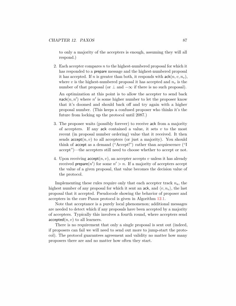
CHAPTER 12. PAXOS 87

to only a majority of the accepters is enough, assuming they will allrespond.)

2. Each accepter compares n to the highest-numbered proposal for which ithas responded to a prepare message and the highest-numbered proposalit has accepted. If n is greater than both, it responds with ack(n, v, nv),where v is the highest-numbered proposal it has accepted and nv is thenumber of that proposal (or ⊥ and −∞ if there is no such proposal).An optimization at this point is to allow the accepter to send backnack(n, n′) where n′ is some higher number to let the proposer knowthat it’s doomed and should back off and try again with a higherproposal number. (This keeps a confused proposer who thinks it’s thefuture from locking up the protocol until 2087.)

3. The proposer waits (possibly forever) to receive ack from a majorityof accepters. If any ack contained a value, it sets v to the mostrecent (in proposal number ordering) value that it received. It thensends accept(n, v) to all accepters (or just a majority). You shouldthink of accept as a demand (“Accept!”) rather than acquiescence (“Iaccept”)—the accepters still need to choose whether to accept or not.

4. Upon receiving accept(n, v), an accepter accepts v unless it has alreadyreceived prepare(n′) for some n′ > n. If a majority of accepters acceptthe value of a given proposal, that value becomes the decision value ofthe protocol.

Implementing these rules require only that each accepter track na, thehighest number of any proposal for which it sent an ack, and 〈v, nv〉, the lastproposal that it accepted. Pseudocode showing the behavior of proposer andaccepters in the core Paxos protocol is given in Algorithm 12.1.

Note that acceptance is a purely local phenomenon; additional messagesare needed to detect which if any proposals have been accepted by a majorityof accepters. Typically this involves a fourth round, where accepters sendaccepted(n, v) to all learners.

There is no requirement that only a single proposal is sent out (indeed,if proposers can fail we will need to send out more to jump-start the proto-col). The protocol guarantees agreement and validity no matter how manyproposers there are and no matter how often they start.

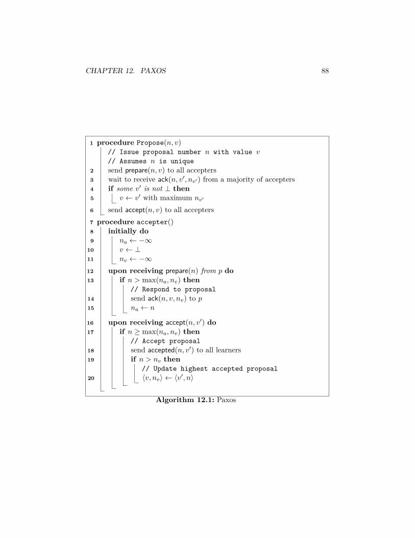
CHAPTER 12. PAXOS 88

1 procedure Propose(n, v)// Issue proposal number n with value v// Assumes n is unique

2 send prepare(n, v) to all accepters3 wait to receive ack(n, v′, nv′) from a majority of accepters4 if some v′ is not ⊥ then5 v ← v′ with maximum nv′

6 send accept(n, v) to all accepters7 procedure accepter()8 initially do9 na ← −∞

10 v ← ⊥11 nv ← −∞12 upon receiving prepare(n) from p do13 if n > max(na, nv) then

// Respond to proposal14 send ack(n, v, nv) to p15 na ← n

16 upon receiving accept(n, v′) do17 if n ≥ max(na, nv) then

// Accept proposal18 send accepted(n, v′) to all learners19 if n > nv then

// Update highest accepted proposal20 〈v, nv〉 ← 〈v′, n〉

Algorithm 12.1: Paxos

CHAPTER 12. PAXOS 89

12.2 Informal analysis: how information flows be-tween rounds

Call a round the collection of all messages labeled with some particularproposal n. The structure of the algorithm simulates a sequential executionin which higher-numbered rounds follow lower-numbered ones, even thoughthere is no guarantee that this is actually the case in a real execution.

When an accepter sends ack(n, v, nv), it is telling the round-n proposerthe last value preceding round n that it accepted. The rule that an accepteronly acknowledges a proposal higher than any proposal it has previouslyaccepted prevents it from sending information “back in time”—the roundnv in an acknowledgment is always less than n. The rule that an accepterdoesn’t accept any proposal earlier than a round it has acknowledged meansthat the value v in an ack(n, v, nv) message never goes out of date—there isno possibility that an accepter might retroactively accept some later value inround n′ with nv < n′ < n. So the ack message values tell a consistent storyabout the history of the protocol, even if the rounds execute out of order.

The second trick is to use overlapping majorities to make sure that anyvalue that is accepted is not lost. If the only way to decide on a value in roundn is to get a majority of accepters to accept it, and the only way to makeprogress in round n′ is to get acknowledgments from a majority of accepters,these two majorities overlap. So in particular the overlapping process reportsthe round-n proposal value to the proposer in round n′, and we can showby induction on n′ that this round-n proposal value becomes the proposalvalue in all subsequent rounds that proceed past the acknowledgment stage.So even though it may not be possible to detect that a decision has beenreached in round n (say, because some of the accepters in the acceptingmajority die without telling anybody what they did), no later round will beable to choose a different value. This ultimately guarantees agreement.

12.2.1 Example execution

For Paxos to work well, proposal numbers should increase over time. Butthere is no requirement that proposal numbers are increasing or even thatproposals with different proposal numbers don’t overlap. When thinkingabout Paxos, it is easy to make the mistake of ignore cases where proposalsare processed concurrently or out of order. In Figure 12.1, we give an exampleof an execution with three proposals running concurrently.

CHAPTER 12. PAXOS 90

p1 p2 p3 a1 a2 a3prepare(3)

prepare(2)prepare(1)

ack(3,⊥, 0)ack(1,⊥, 0)

ack(1,⊥, 0)accept(1, 1)

accepted(1, 1)nack(1, 3)

ack(2, 1, 1)ack(2,⊥, 0)

accept(2, 1)nack(2, 3)

accepted(2, 1)ack(3, 1, 2)

accept(3, 1)accepted(3, 1)

accepted(3, 1)

Figure 12.1: Example execution of Paxos. There are three proposers p1, p2,and p3 and three accepters a1, a2, and a3. Proposer p1’s proposed value 1 isnot accepted by a majority of processes in round 1, but it is picked up byproposer p2 in round 2, and is eventually adopted and accepted in round 3.

CHAPTER 12. PAXOS 91

12.2.2 Safety properties

We now present a more formal analysis of the Paxos protocol. We consideronly the safety properties of the protocol, corresponding to validity andagreement. Without additional assumptions, Paxos does not guaranteetermination.

Call a value chosen if it is accepted by a majority of accepters. Thesafety properties of Paxos are:

• No value is chosen unless it is first proposed. (This gives validity.)

• No two distinct values are both chosen. (This gives agreement.)

The first property is immediate from examination of the algorithm:every value propagated through the algorithm is ultimately a copy of someproposer’s original input. We can formalize this observation by checking that,for any set of values S, the property that all values contained in messages orprocesses’ internal state are in S is an invariant.

For the second property, we’ll show by induction on proposal numberthat a value v chosen with proposal number n is the value chosen by anyproposer pn′ with proposal number n′. There are two things that make thistrue:

1. Any ack(n′, v′, nv′) message received by pn′ has nv′ < n′. Proof: Im-mediate from the code.

2. If a majority of accepters accept a proposal with number n at somepoint during the execution, and pn′ receives ack(n′,−,−) messages froma majority of accepters, then pn′ receives at least one ack(n′, v′, nv′)message with n′ ≥ n. Proof: Let S be the set of processes that issueaccepted(n, v) and let T be the set of processes that send ack(n′,−,−)to p′. Because S and T are both majorities, there is at least oneaccepter a in S ∩ T . Suppose pn′ receives ack(n, v′′, n′′) from a. Ifn′′ < n, then at the time a sends its ack(n, v′′, n′′) message, it has notyet accepted a proposal with number n. But then when it does receiveaccept(n, v), it rejects it. This contradicts a ∈ S.

These two properties together imply that pn′ receives at least oneack(n, v′′, n′′) with n ≤ n′′ < n′ and no such messages with n′′ < n. Sothe maximum proposal number it sees is n′′ where n ≤ n′′ < n. By theinduction hypothesis, the corresponding value is v. It follows that pn′ alsochooses v.

CHAPTER 12. PAXOS 92

12.2.3 Learning the results

Somebody has to find out that a majority accepted a proposal in order to geta decision value out. The usual way to do this is to have a fourth round ofmessages where the accepters send accepted(v, n) to some designated learners.These are often the processes that need to implement whatever decision wasmade by the agreement protocol, but in principle could be any processesthat care about the outcome.

12.2.4 Liveness properties

We’d like the protocol to terminate eventually. Suppose there is a singleproposer, and that it survives long enough to collect a majority of acks and tosend out accepts to a majority of the accepters. If everybody else cooperates,we get termination in 4 message delays, including the time for the learnersto detect acceptance.

If there are multiple proposers, then they can step on each other. Forexample, it’s enough to have two carefully-synchronized proposers alternatesending out prepare messages to prevent any accepter from every accepting(since an accepter promises not to accept accept(n, v) once it has respondedto prepare(n+ 1)). The solution is to ensure that there is eventually someinterval during which there is exactly one proposer who doesn’t fail. One wayto do this is to use exponential random backoff (as popularized by Ethernet):when a proposer decides it’s not going to win a round (e.g., by receiving anack or by waiting long enough to realize it won’t be getting any more ackssoon), it picks some increasingly large random delay before starting a newround. Unless something strange is going on, new rounds will eventuallystart far enough apart in time that one will get done without interference.

A more abstract solution is to assume some sort of weak leader electionmechanism, which tells each accepter who the “legitimate” proposer is ateach time. The accepters then discard messages from illegitimate proposers,which prevents conflict at the cost of possibly preventing progress. Progressis however obtained if the mechanism eventually reaches a state where amajority of the accepters bow to the same non-faulty proposer long enoughfor the proposal to go through.

Such a weak leader election method is an example of a more general classof mechanisms known as failure detectors, in which each process gets hintsabout what other processes are faulty that eventually converge to reality.The weak-leader-election failure detector needed for Paxos is called the Ωfailure detector. There are other still weaker failure detectors that can also

CHAPTER 12. PAXOS 93

be used to solve consensus. We will discuss failure detectors in detail inChapter 13.

12.3 Replicated state machines and multi-PaxosThe most common practical use of Paxos is to implement a replicatedstate machine [Lam78]. The idea is to maintain many copies of some datastructure, each on a separate machine, and guarantee that each copy (orreplica) stays in sync with all the others as new operations are appliedto them. This requires some mechanism to ensure that all the differentreplicas apply the same sequence of operations, or in other words that themachines that hold the replicas solve a sequence of agreement problems toagree on these operations. The payoff is that the state of the data structuresurvives the failure of some of the machines, without having to copy theentire structure every time it changes.

Making all copies consistent requires solving a new version of agreementevery time we want to add another operation. Paxos works well for thisbecause we can have to proposer simply issue a new proposal without takinginto account any lower-numbered values, assuming that it has verified thatlower-numbered values have in fact been accepted. The round-numbermechanism means that all of the accepters will switch to working on the newproposal without any modifications to their code.

Typically for this application, we’ll have a single active proposer that isresponsible for serializing any incoming operations to the replicated statemachine. If the proposer doesn’t change very often, a further optimizationallows skipping the prepare and ack messages in between agreement protocolsfor consecutive operations. This reduces the time to certify each operationto a single round-trip for the accept and accepted messages, which is aboutthe best we can reasonably hope for.

One detail is that to make this work, we need to distinguish betweenconsecutive proposals by the same proposer, and “new” proposals that changethe proposer in addition to reaching agreement on some value. This is doneby splitting the proposal number into a major and minor number, withproposals ordered lexicographically. A proposer that wins 〈x, 0〉 is allowed tomake further proposals numbered 〈x, 1〉 , 〈x, 2〉 , etc. But a different proposerwill need to increment x.

Lamport calls this optimization Paxos in [Lam01]; other authors havecalled it multi-Paxos to distinguish it from the basic Paxos algorithm.

Chapter 13

Failure detectors

Failure detectors were proposed by Chandra and Toueg [CT96] as a mech-anism for solving consensus in an asynchronous message-passing system withcrash failures by distinguishing between slow processes and dead processes.The basic idea is that each process has attached to it a failure detector modulethat continuously outputs an estimate of which processes in the system havefailed. The output need not be correct; indeed, the main contribution ofChandra and Toueg’s paper (and a companion paper by Chandra, Hadzilacos,and Toueg [CHT96]) is characterizing just how bogus the output of a failuredetector can be and still be useful.

We will mostly follow Chandra and Toueg in these notes; see the paperfor the full technical details.

To emphasize that the output of a failure detector is merely a hint atthe actual state of the world, a failure detector (or the process it’s attachedto) is said to suspect a process at time t if it outputs failed at that time.Failure detectors can then be classified based on when their suspicions arecorrect.

We use the usual asynchronous message-passing model, and in particularassume that non-faulty processes execute infinitely often, get all their mes-sages delivered, etc. From time to time we will need to talk about time, andunless we are clearly talking about real time this just means any steadilyincreasing count (e.g., of total events), and will be used only to describe theordering of events.

94

CHAPTER 13. FAILURE DETECTORS 95

13.1 How to build a failure detectorFailure detectors are only interesting if you can actually build them. Ina fully asynchronous system, you can’t (this follows from the FLP resultand the existence of failure-detector-based consensus protocols). But withtimeouts, it’s not hard: have each process ping each other process fromtime to time, and suspect the other process if it doesn’t respond to the pingwithin twice the maximum round-trip time for any previous ping. Assumingthat ping packets are never lost and there is an (unknown) upper bound onmessage delay, this gives what is known as an eventually perfect failuredetector: once the max round-trip times rise enough and enough time haselapsed for the live processes to give up on the dead ones, all and only deadprocesses are suspected.

13.2 Classification of failure detectorsChandra and Toueg define eight classes of failure detectors, based on whenthey suspect faulty processes and non-faulty processes. Suspicion of faultyprocesses comes under the heading of completeness; of non-faulty processes,accuracy.

13.2.1 Degrees of completeness

Strong completeness Every faulty process is eventually permanently sus-pected by every non-faulty process.

Weak completeness Every faulty process is eventually permanently sus-pected by some non-faulty process.

There are two temporal logic operators embedded in these statements:“eventually permanently” means that there is some time t0 such that forall times t ≥ t0, the process is suspected. Note that completeness saysnothing about suspecting non-faulty processes: a paranoid failure detectorthat permanently suspects everybody has strong completeness.

13.2.2 Degrees of accuracy

These describe what happens with non-faulty processes, and with faultyprocesses that haven’t crashed yet.

Strong accuracy No process is suspected (by anybody) before it crashes.

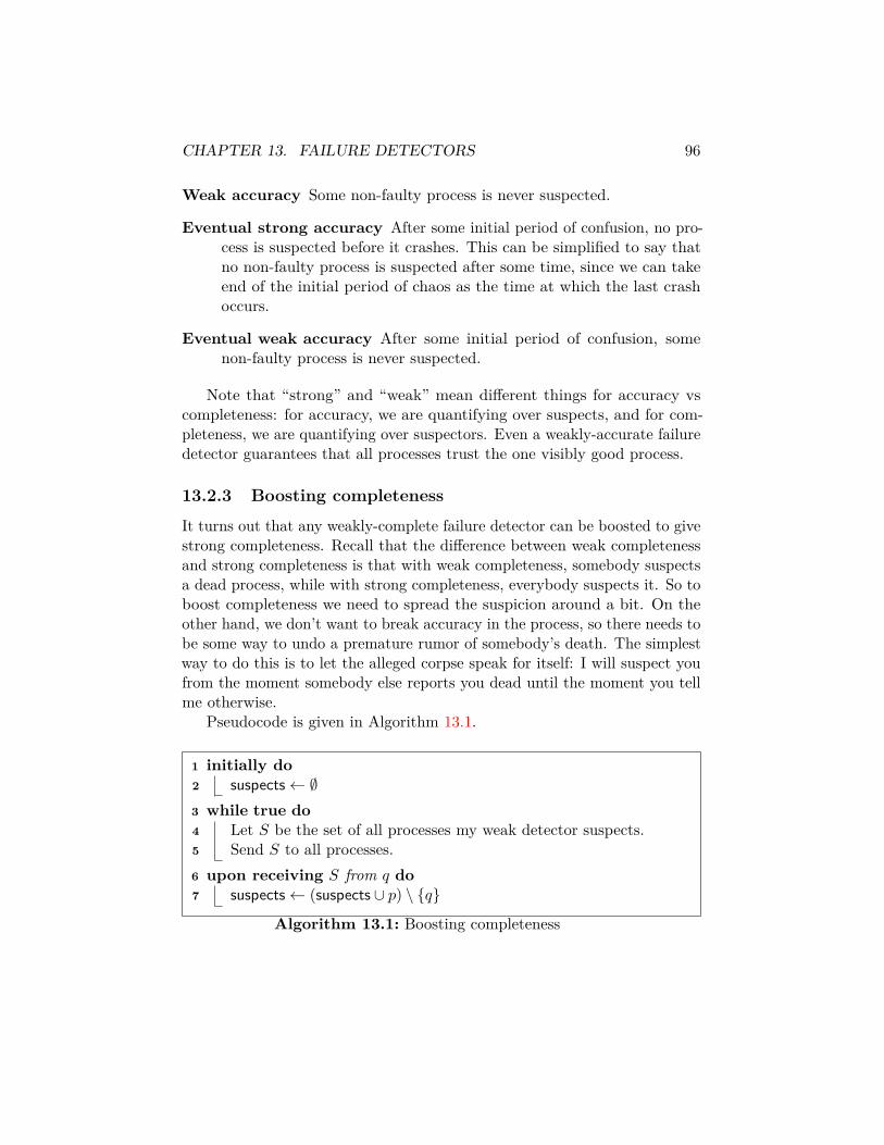
CHAPTER 13. FAILURE DETECTORS 96

Weak accuracy Some non-faulty process is never suspected.

Eventual strong accuracy After some initial period of confusion, no pro-cess is suspected before it crashes. This can be simplified to say thatno non-faulty process is suspected after some time, since we can takeend of the initial period of chaos as the time at which the last crashoccurs.

Eventual weak accuracy After some initial period of confusion, somenon-faulty process is never suspected.

Note that “strong” and “weak” mean different things for accuracy vscompleteness: for accuracy, we are quantifying over suspects, and for com-pleteness, we are quantifying over suspectors. Even a weakly-accurate failuredetector guarantees that all processes trust the one visibly good process.

13.2.3 Boosting completeness

It turns out that any weakly-complete failure detector can be boosted to givestrong completeness. Recall that the difference between weak completenessand strong completeness is that with weak completeness, somebody suspectsa dead process, while with strong completeness, everybody suspects it. So toboost completeness we need to spread the suspicion around a bit. On theother hand, we don’t want to break accuracy in the process, so there needs tobe some way to undo a premature rumor of somebody’s death. The simplestway to do this is to let the alleged corpse speak for itself: I will suspect youfrom the moment somebody else reports you dead until the moment you tellme otherwise.

Pseudocode is given in Algorithm 13.1.

1 initially do2 suspects← ∅3 while true do4 Let S be the set of all processes my weak detector suspects.5 Send S to all processes.6 upon receiving S from q do7 suspects← (suspects ∪ p) \ q

Algorithm 13.1: Boosting completeness

CHAPTER 13. FAILURE DETECTORS 97

It’s not hard to see that this boosts completeness: if p crashes, somebody’sweak detector eventually suspects it, this process tells everybody else, and pnever contradicts it. So eventually everybody suspects p.

What is slightly trickier is showing that it preserves accuracy. Theessential idea is this: if there is some good-guy process p that everybody trustsforever (as in weak accuracy), then nobody ever reports p as suspect—thisalso covers strong accuracy since the only difference is that now every non-faulty process falls into this category. For eventual weak accuracy, waitfor everybody to stop suspecting p, wait for every message ratting out pto be delivered, and then wait for p to send a message to everybody. Noweverybody trusts p, and nobody every suspects p again. Eventual strongaccuracy is again similar.

This will justify ignoring the weakly-complete classes.

13.2.4 Failure detector classes

Two degrees of completeness times four degrees of accuracy gives eight classesof failure detectors, each of which gets its own name. But since we can boostweak completeness to strong completeness, we can use this as an excuse toconsider only the strongly-complete classes.

P (perfect) Strongly complete and strongly accurate: non-faulty processesare never suspected; faulty processes are eventually suspected by ev-erybody. Easily achieved in synchronous systems.

S (strong) Strongly complete and weakly accurate. The name is misleadingif we’ve already forgotten about weak completeness, but the correspond-ing W (weak) class is only weakly complete and weakly accurate, soit’s the strong completeness that the S is referring to.

♦P (eventually perfect) Strongly complete and eventually strongly accu-rate.

♦S (eventually strong) Strongly complete and eventually weakly accu-rate.

Jumping to the punch line: P can simulate any of the others, S and♦P can both simulate ♦S but can’t simulate P or each other, and ♦S can’tsimulate any of the others (See Figure 13.1—we’ll prove all of this later.)Thus ♦S is the weakest class of failure detectors in this list. However, ♦S isstrong enough to solve consensus, and in fact any failure detector (whatever

CHAPTER 13. FAILURE DETECTORS 98

P

S ♦P

♦S

Figure 13.1: Partial order of failure detector classes. Higher classes cansimulate lower classes but not vice versa.

its properties) that can solve consensus is strong enough to simulate ♦S(this is the result in the Chandra-Hadzilacos-Toueg paper [CHT96])—thismakes ♦S the “weakest failure detector for solving consensus” as advertised.Continuing our tour through Chandra and Toueg [CT96], we’ll show thesimulation results and that ♦S can solve consensus, but we’ll skip the ratherinvolved proof of ♦S’s special role from Chandra-Hadzilacos-Toueg.

13.3 Consensus with S

With the strong failure detector S, we can solve consensus for any numberof failures.

In this model, the failure detectors as applied to most processes arecompletely useless. However, there is some non-faulty process c that nobodyevery suspects, and this is enough to solve consensus with as many as n− 1failures.

The basic idea of the protocol: There are three phases. In the first phase,the processes gossip about input values for n− 1 asynchronous rounds. Inthe second, they exchange all the values they’ve seen and prune out anythat are not universally known. In the third, each process decides on thelowest-id input that hasn’t been pruned (minimum input also works since atthis point everybody has the same view of the inputs).

Pseudocode is given in Algorithm 13.2In Phase 1, each process p maintains two partial functions Vp and δp,

where Vp lists all the input values 〈q, vq〉 that p has ever seen and δp listsonly those input values seen in the most recent of n− 1 asynchronous rounds.Both Vp and δp are initialized to 〈p, vp〉. In round i, p sends (i, δp) to allprocesses. It then collects 〈i, δq〉 from each q that it doesn’t suspect and setsδp to

⋃q δq \ Vp (where q ranges over the processes from which p received a

CHAPTER 13. FAILURE DETECTORS 99

1 Vp ← 〈p, vp〉2 δp ← 〈p, vp〉

// Phase 13 for i← 1 to n− 1 do4 Send 〈i, δp〉 to all processes.5 Wait to receive 〈i, δq〉 from all q I do not suspect.6 δp ←

(⋃q δq

)\ Vp

7 Vp ←(⋃

q δq)∪ Vp

// Phase 28 Send 〈n, Vp〉 to all processes.9 Wait to receive 〈n, Vq〉 from all q I do not suspect.

10 Vp ←(⋂

q Vq)∩ Vp

// Phase 311 return some input from Vp chosen via a consistent rule.

Algorithm 13.2: Consensus with a strong failure detector

message in round i) and sets Vp to Vp ∪ δp. In the next round, it repeats theprocess. Note that each pair 〈q, vq〉 is only sent by a particular process p thefirst round after p learns it: so any value that is still kicking around in roundn− 1 had to go through n− 1 processes.

In Phase 2, each process p sends 〈n, Vp〉, waits to receive 〈n, Vq〉 fromevery process it does not suspect, and sets Vp to the intersection of Vp andall received Vq. At the end of this phase all Vp values will in fact be equal,as we will show.

In Phase 3, everybody picks some input from their Vp vector accordingto a consistent rule.

13.3.1 Proof of correctness

Let c be a non-faulty process that nobody every suspects.The first observation is that the protocol satisfies validity, since every

Vp contains vc after round 1 and each Vp can only contain input values byexamination of the protocol. Whatever it may do to the other values, takingintersections in Phase 2 still leaves vc, so all processes pick some input valuefrom a nonempty list in Phase 3.

To get termination we have to prove that nobody ever waits foreverfor a message it wants; this basically comes down to showing that the first

CHAPTER 13. FAILURE DETECTORS 100

non-faulty process that gets stuck eventually is informed by the S-detectorthat the process it is waiting for is dead.

For agreement, we must show that in Phase 3, every Vp is equal; inparticular, we’ll show that every Vp = Vc. First it is necessary to show thatat the end of Phase 1, Vc ⊆ Vp for all p. This is done by considering twocases:

1. If 〈q, vq〉 ∈ Vc and c learns 〈q, vq〉 before round n − 1, then c sends〈q, vq〉 to p no later than round n− 1, p waits for it (since nobody eversuspects c), and adds it to Vp.

2. If 〈q, vq〉 ∈ Vc and c learns 〈q, vq〉 only in round n− 1, then 〈q, vq〉 waspreviously sent through n− 1 other processes, i.e., all of them. Eachprocess p 6= c thus added 〈q, vq〉 to Vp before sending it and again〈q, vq〉 is in Vp.

(The missing case where 〈q, vq〉 isn’t in Vc we don’t care about.)But now Phase 2 knocks out any extra elements in Vp, since Vp gets set to

Vp ∩ Vc ∩ (some other Vq’s that are supersets of Vc). It follows that, at theend of Phase 2, Vp = Vc for all p. Finally, in Phase 3, everybody applies thesame selection rule to these identical sets and we get agreement.

13.4 Consensus with ♦S and f < n/2The consensus protocol for S depends on some process c never being suspected;if c is suspected during the entire (finite) execution of the protocol—as canhappen with ♦S—then it is possible that no process will wait to hear fromc (or anybody else) and the processes will all decide their own inputs. Soto solve consensus with ♦S we will need to assume fewer than n/2 failures,allowing any process to wait to hear from a majority no matter what lies itsfailure detector is telling it.

The resulting protocol, known as the Chandra-Toueg consensus pro-tocol, is structurally similar to the consensus protocol in Paxos.1 Thedifference is that instead of proposers blindly showing up, the protocol isdivided into rounds with a rotating coordinator pi in each round r withr = i (mod n). The termination proof is based on showing that in any roundwhere the coordinator is not faulty and nobody suspects it, the protocolfinishes.

1See Chapter 12.

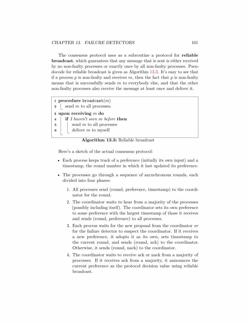
CHAPTER 13. FAILURE DETECTORS 101

The consensus protocol uses as a subroutine a protocol for reliablebroadcast, which guarantees that any message that is sent is either receivedby no non-faulty processes or exactly once by all non-faulty processes. Pseu-docode for reliable broadcast is given as Algorithm 13.3. It’s easy to see thatif a process p is non-faulty and receives m, then the fact that p is non-faultymeans that is successfully sends m to everybody else, and that the othernon-faulty processes also receive the message at least once and deliver it.

1 procedure broadcast(m)2 send m to all processes.3 upon receiving m do4 if I haven’t seen m before then5 send m to all processes6 deliver m to myself

Algorithm 13.3: Reliable broadcast

Here’s a sketch of the actual consensus protocol:

• Each process keeps track of a preference (initially its own input) and atimestamp, the round number in which it last updated its preference.

• The processes go through a sequence of asynchronous rounds, eachdivided into four phases:

1. All processes send (round, preference, timestamp) to the coordi-nator for the round.

2. The coordinator waits to hear from a majority of the processes(possibly including itself). The coordinator sets its own preferenceto some preference with the largest timestamp of those it receivesand sends (round, preference) to all processes.

3. Each process waits for the new proposal from the coordinator orfor the failure detector to suspect the coordinator. If it receivesa new preference, it adopts it as its own, sets timestamp tothe current round, and sends (round, ack) to the coordinator.Otherwise, it sends (round, nack) to the coordinator.

4. The coordinator waits to receive ack or nack from a majority ofprocesses. If it receives ack from a majority, it announces thecurrent preference as the protocol decision value using reliablebroadcast.

CHAPTER 13. FAILURE DETECTORS 102

• Any process that receives a value in a reliable broadcast decides on itimmediately.

Pseudocode is in Algorithm 19.

1 preference← input2 timestamp← 03 for round← 1 . . .∞ do4 Send 〈round, preference, timestamp〉 to coordinator5 if I am the coordinator then6 Wait to receive 〈round, preference, timestamp〉 from majority

of processes.7 Set preference to value with largest timestamp.8 Send 〈round, preference〉 to all processes.9 Wait to receive

⟨round, preference′

⟩from coordinator or to suspect

coordinator.10 if I received

⟨round, preference′

⟩then

11 preference← preference′12 timestamp← round13 Send ack(round) to coordinator.14 else15 Send nack(round) to coordinator.16 if I am the coordinator then17 Wait to receive ack(round) or nack(round) from a majority of

processes.18 if I received no nack(round) messages then19 Broadcast preference using reliable broadcast.

13.4.1 Proof of correctness

For validity, observe that the decision value is an estimate and all estimatesstart out as inputs.

For termination, observe that no process gets stuck in Phase 1, 2, or 4,because either it isn’t waiting or it is waiting for a majority of non-faultyprocesses who all sent messages unless they have already decided (this iswhy we need the nacks in Phase 3). The loophole here is that processes thatdecide stop participating in the protocol; but because any non-faulty process

CHAPTER 13. FAILURE DETECTORS 103

retransmits the decision value in the reliable broadcast, if a process is waitingfor a response from a non-faulty process that already terminated, eventuallyit will get the reliable broadcast instead and terminate itself. In Phase 3,a process might get stuck waiting for a dead coordinator, but the strongcompleteness of ♦S means that it suspects the dead coordinator eventuallyand escapes. So at worst we do finitely many rounds.

Now suppose that after some time t there is a process c that is neversuspected by any process. Then in the next round in which c is the coordi-nator, in Phase 3 all surviving processes wait for c and respond with ack, cdecides on the current estimate, and triggers the reliable broadcast protocolto ensure everybody else decides on the same value. Since reliable broadcastguarantees that everybody receives the message, everybody decides this valueor some value previously broadcast—but in either case everybody decides.

Agreement is the tricky part. It’s possible that two coordinators bothinitiate a reliable broadcast and some processes choose the value from the firstand some the value from the second. But in this case the first coordinatorcollected acks from a majority of processes in some round r, and all subsequentcoordinators collected estimates from an overlapping majority of processes insome round r′ > r. By applying the same induction argument as for Paxos,we get that all subsequent coordinators choose the same estimate as the firstcoordinator, and so we get agreement.

13.5 f < n/2 is still required even with ♦P

We can show that with a majority of failures, we’re in trouble with just ♦P(and thus with ♦S, which is trivially simulated by ♦P ). The reason is that♦P can lie to us for some long initial interval of the protocol, and consensusis required to terminate eventually despite these lies. So the usual partitionargument works: start half of the processes with input 0, half with 1, andrun both halves independently with ♦P suspecting the other half until theprocesses in both halves decide on their common inputs. We can now make♦P happy by letting it stop suspecting the processes, but it’s too late.

13.6 Relationships among the classesIt’s easy to see that P simulates S and ♦P simulates ♦S without modification.It’s also immediate that P simulates ♦P and S simulates ♦S (make “even-tually” be “now”), which gives a diamond-shaped lattice structure betweenthe classes. What is trickier is to show that this structure doesn’t collapse:

CHAPTER 13. FAILURE DETECTORS 104

♦P can’t simulate S, S can’t simulate ♦P , and ♦S can’t simulate any of theother classes.

First let’s observe that ♦P can’t simulate S: if it could, we would get aconsensus protocol for f ≥ n/2 failures, which we can’t do. It follows that♦P also can’t simulate P (because P can simulate S).

To show that S can’t simulate ♦P , choose some non-faulty victim processv and consider an execution in which S periodically suspects v (which itis allowed to do as long as there is some other non-faulty process it neversuspects). If the ♦P -simulator ever responds to this by refusing to suspect v,there is an execution in which v really is dead, and the simulator violatesstrong completeness. But if not, we violate eventual strong accuracy. Notethat this also implies S can’t simulate P , since P can simulate ♦P . It alsoshows that ♦S can’t simulate either of ♦P or P .

We are left with showing ♦S can’t simulate S. Consider a system wherep’s ♦S detector suspects q but not r from the start of the execution, andsimilarly r’s ♦S detector also suspects q but not p. Run p and r in isolationuntil they give up and decide that q is in fact dead (which they must doeventually by strong completeness, since this run is indistinguishable fromone in which q is faulty). Then wake up q and crash p and r. Since q is theonly non-faulty process, we’ve violated weak accuracy.

Chandra and Toueg [CT96] give as an example of a natural problemthat can be solved only with P the problem of terminating reliablebroadcast, in which a single leader process attempts to send a message andall other processes eventually agree on the message if the leader is non-faultybut must terminate after finite time with a default no message return valueif the leader is faulty.2 The process is solvable using P by just having eachprocess either wait for the message or for P to suspect the leader, which canonly occur if the leader does in fact crash. If the leader is dead, the processesmust eventually decide on no message; this separates P from ♦S and ♦Psince we can then wake up the leader and let it send its message. But it alsoseparates P from S, since we can have the S-detector only be accurate fornon-leaders. For other similar problems see the paper.

2This is a slight weakening of the problem, which however still separates P from theother classes. For the real problem see Chandra and Toueg [CT96].

Chapter 14

Quorum systems

Last updated 2014. Some material may be out of date.

14.1 BasicsIn the past few chapters, we’ve seen many protocols that depend on thefact that if I talk to more than n/2 processes and you talk to more thann/2 processes, the two groups overlap. This is a special case of a quorumsystem, a family of subsets of the set of processes with the property thatany two subsets in the family overlap. By choosing an appropriate family, wemay be able to achieve lower load on each system member, higher availability,defense against Byzantine faults, etc.

The exciting thing from a theoretical perspective is that these turna systems problem into a combinatorial problem: this means we can askcombinatorialists how to solve it.

14.2 Simple quorum systems• Majority and weighted majorities

• Specialized read/write systems where write quorum is a column andread quorum a row of some grid.

• Dynamic quorum systems: get more than half of the most recent copy.

• Crumbling walls [PW97b, PW97a]: optimal small-quorum system forgood choice of wall sizes.

105

CHAPTER 14. QUORUM SYSTEMS 106

14.3 Goals• Minimize quorum size.

• Minimize load, defined as the minimum over all access strategies(probability distributions on quorums) of the maximum over all serversof probability it gets hit.

• Maximize capacity, defined as the maximum number of quorum ac-cesses per time unit in the limit if each quorum access ties up a quorummember for 1 time unit (but we are allowed to stagger a quorum accessover multiple time units).

• Maximize fault-tolerance: minimum number of server failures thatblocks all quorums. Note that for standard quorum systems this isdirectly opposed to minimizing quorum size, since killing the smallestquorum stops us dead.

• Minimize failure probability = probability that every quorum con-tains at least one bad server, assuming each server fails with independentprobability.

Naor and Wool [NW98] describe trade-offs between these goals (some ofthese were previously known, see the paper for citations):

• capacity = 1/load; this is obtained by selecting the quorums indepen-dently at random according to the load-minimizing distribution. Inparticular this means we can forget about capacity and just concentrateon minimizing load.

• load ≥ max(c/n, 1/c) where c is the minimum quorum size. The firstcase is obvious: if every access hits c nodes, spreading them out asevenly as possible still hits each node c/n of the time. The second istrickier: Naor and Wool prove it using LP duality, but the argumentessentially says that if we have some quorum Q of size c, then sinceevery other quorum Q′ intersects Q in at least one place, we can showthat every Q′ adds at least 1 unit of load in total to the c members ofQ. So if we pick a random quorum Q′, the average load added to all ofQ is at least 1, so the average load added to some particular elementof Q is at least 1/|Q| = 1/c. Combining the two cases, we can’t hopeto get load better than 1/

√n, and to get this load we need quorums of

size at least√n.

CHAPTER 14. QUORUM SYSTEMS 107

Figure 14.1: Figure 2 from [NW98]. Solid lines are G(3); dashed lines areG∗(3).

• failure probability is at least p when p > 1/2 (and optimal system is tojust pick a single leader in this case), failure probability can be madeexponentially small in size of smallest quorum when p < 1/2 (withmany quorums). These results are due to Peleg and Wool [PW95].

14.4 Paths systemThis is an optimal-load system from Naor and Wool [NW98] with exponen-tially low failure probability, based on percolation theory.

The basic idea is to build a d×d mesh-like graph where a quorum consistsof the union of a top-to-bottom path (TB path) and a left-to-right path (LRpath); this gives quorum size O(

√n) and load O(1/

√n). Note that the TB

and LR paths are not necessarily direct: they may wander around for a whilein order to get where they are going, especially if there are a lot of failuresto avoid. But the smallest quorums will have size 2d+ 1 = O(

√n).

The actual mesh is a little more complicated. Figure 14.1 reproduces thepicture of the d = 3 case from the Naor and Wool paper.

Each server corresponds to a pair of intersecting edges, one from the

CHAPTER 14. QUORUM SYSTEMS 108

G(d) grid and one from the G∗(d) grid (the star indicates that G∗(d) is thedual graph1 of G(d). A quorum consists of a set of servers that produce anLR path in G(d) and a TB path in G∗(d). Quorums intersect, because anyLR path in G(d) must cross some TB path in G∗(d) at some server (in fact,each pair of quorums intersects in at least two places). The total number ofelements n is (d+ 1)2 and the minimum size of a quorum is 2d+ 1 = Θ(

√n).

The symmetry of the mesh gives that there exists a LR path in themesh if and only if there does not exist a TB path in its complement, thegraph that has an edge only if the mesh doesn’t. For a mesh with failureprobability p < 1/2, the complement is a mesh with failure probabilityq = 1− p > 1/2. Using results in percolation theory, it can be shown that forfailure probability q > 1/2, the probability that there exists a left-to-rightpath is exponentially small in d (formally, for each p there is a constant φ(p)such that Pr[∃LR path] ≤ exp(−φ(p)d)). We then have

Pr[∃(live quorum)] = Pr[∃(TB path) ∧ ∃(LR path)]= Pr[¬∃(LR path in complement) ∨ ¬∃(TB path in complement)]≤ Pr[¬∃(LR path in complement)] + Pr[¬∃(TB path in complement)]≤ 2 exp(−φ(1− p)d)= 2 exp(−Θ(

√n)).

So the failure probability of this system is exponentially small for any fixedp < 1/2.

See the paper [NW98] for more details.

14.5 Byzantine quorum systemsStandard quorum systems are great when you only have crash failures, butwith Byzantine failures you have to worry about finding a quorum thatincludes a Byzantine serve who lies about the data. For this purpose youneed something stronger. Following Malkhi and Reiter [MR98] and Malkhi etal. [MRWW01], one can define:

• A b-disseminating quorum system guarantees |Q1 ∩Q2| ≥ b +1 for all quorums Q1 and Q2. This guarantees that if I update a

1See http://en.wikipedia.org/wiki/Dual_graph; the basic idea is that the dual of agraph G embedded in the plane has a vertex for each region of G, and an edge connectingeach pair of vertices corresponding to adjacent regions, where a region is a subset of theplane that is bounded by edges of G.

CHAPTER 14. QUORUM SYSTEMS 109

quorum Q1 and you update a quorum Q2, and there are at mostb Byzantine processes, then there is some non-Byzantine process inboth our quorums. Mostly useful if data is “self-verifying,” that is,signed with digital signatures that the Byzantine processes can’t forge.Otherwise, I can’t tell which of the allegedly most recent data values isthe right one since the Byzantine processes lie.

• A b-masking quorum system guarantees |Q1 ∩Q2| ≥ 2b + 1 forall quorums Q1 and Q2. (In other words, it’s the same as a 2b-disseminating quorum system.) This allows me to defeat the Byzantineprocesses through voting: given 2b+ 1 overlapping servers, if I wantthe most recent value of the data I take the one with the most recenttimestamp that appears on at least b+ 1 servers, which the Byzantineguys can’t fake.

An additional requirement in both cases is that for any set of servers Bwith |B| ≤ b, there is some quorum Q such that Q ∩B = ∅. This preventsthe Byzantine processes from stopping the system by simply refusing toparticipate.

Note: these definitions are based on the assumption that there is somefixed bound on the number of Byzantine processes. Malkhi and Reiter [MR98]give more complicated definitions for the case where one has an arbitraryfamily B of potential Byzantine sets. The definitions above are actuallysimplified versions from [MRWW01].

The simplest way to build a b-disseminating quorum system is to usesupermajorities of size at least (n+ b+ 1)/2; the overlap between any twosuch supermajorities is at least (n+ b+ 1)− n = b+ 1. This gives a load ofsubstantially more than 1

2 . There are better constructions that knock theload down to Θ(

√b/n); see [MRWW01].

For more on this topic in general, see the survey by by Merideth andReiter [MR10].

14.6 Probabilistic quorum systemsThe problem with all standard (or strict) quorum systems is that we need bigquorums to get high fault tolerance, since the adversary can always stop usby knocking out our smallest quorum. A probabilistic quorum system ormore specifically an ε-intersecting quorum system [MRWW01] improvesthe fault-tolerance by relaxing the requirements. For such a system we havenot only a set system Q, but also a probability distribution w supplied by

CHAPTER 14. QUORUM SYSTEMS 110

the quorum system designer, with the property that Pr[Q1 ∩ Q2 = ∅] ≤ εwhen Q1 and Q2 are chosen independently according to their weights.

14.6.1 Example

Let a quorum be any set of size k√n for some k and let all quorums be

chosen uniformly at random. Pick some quorum Q1; what is the probabilitythat a random Q2 does not intersect Q1? Imagine we choose the elementsof Q2 one at a time. The chance that the first element x1 of Q2 misses Q1is exactly (n − k

√n)/n = 1 − k/

√n, and conditioning on x1 through xi−1

missing Q1 the probability that xi also misses it is (n− k√n− i+ 1)/(n−

i + 1) ≤ (n − k√n)/n = 1 − k/

√n. So taking the product over all i gives

Pr[all miss Q1] ≤ (1 − k/√n)k√n ≤ exp(−k

√n)k/

√n) = exp(−k2). So by

setting k = Θ(ln 1/ε), we can get our desired ε-intersecting system.

14.6.2 Performance

Failure probabilities, if naively defined, can be made arbitrarily small: addlow-probability singleton quorums that are hardly ever picked unless massivefailures occur. But the resulting system is still ε-intersecting.

One way to look at this is that it points out a flaw in the ε-intersectingdefinition: ε-intersecting quorums may cease to be ε-intersecting conditionedon a particular failure pattern (e.g., when all the non-singleton quorums areknocked out by massive failures). But Malkhi et al. [MRWW01] address theproblem in a different way, by considering only survival of high qualityquorums, where a particular quorum Q is δ-high-quality if Pr[Q1 ∩Q2 =∅|Q1 = Q] ≤ δ and high quality if it’s

√ε-high-quality. It’s not hard to show

that a random quorum is δ-high-quality with probability at least ε/δ, so ahigh quality quorum is one that fails to intersect a random quorum withprobability at most

√ε and a high quality quorum is picked with probability

at least 1−√ε.

We can also consider load; Malkhi et al. [MRWW01] show that essentiallythe same bounds on load for strict quorum systems also hold for ε-intersectingquorum systems: load(S) ≥ max((E(|Q|)/n, (1−

√ε)2/E(|Q|)), where E(|Q|)

is the expected size of a quorum. The left-hand branch of the max is justthe average load applied to a uniformly-chosen server. For the right-handside, pick some high quality quorum Q′ with size less than or equal to(1−

√ε) E(|Q|) and consider the load applied to its most loaded member by

its nonempty intersection (which occurs with probability at least 1 −√ε)

with a random quorum.

CHAPTER 14. QUORUM SYSTEMS 111

14.7 Signed quorum systemsA further generalization of probabilistic quorum systems gives signed quo-rum systems [Yu06]. In these systems, a quorum consists of some set ofpositive members (servers you reached) and negative members (servers youtried to reach but couldn’t). These allow O(1)-sized quorums while toleratingn−O(1) failures, under certain natural probabilistic assumptions. Becausethe quorums are small, the load on some servers may be very high: so theseare most useful for fault-tolerance rather than load-balancing. See the paperfor more details.

Part II

Shared memory

112

Chapter 15

Model

Shared memory models describe the behavior of processes in a multiprocessingsystem. These processes might correspond to actual physical processors orprocessor cores, or might use time-sharing on a single physical processor. Ineither case the assumption is that communication is through some sort ofshared data structures.

Here we describe the basic shared-memory model. See also [AW04, §4.1].The idea of shared memory is that instead of sending messages to each

other, processes communicate through a pool of shared objects. These aretypically registers supporting read and write operations, but fancier objectscorresponding to more sophisticated data structures or synchronizationprimitives may also be included in the model.

It is usually assumed that the shared objects do not experience faults.This means that the shared memory can be used as a tool to prevent partitionsand other problems that can arise in message passing if the number of faultsget too high. As a result, for large numbers of processor failures, sharedmemory is a more powerful model than message passing, although we will seein Chapter 16 that both models can simulate each other provided a majorityof processes are non-faulty.

15.1 Atomic registersAn atomic register supports read and write operations; we think of theseas happening instantaneously, and think of operations of different processesas interleaved in some sequence. Each read operation on a particular reg-ister returns the value written by the last previous write operation. Writeoperations return nothing.

113

CHAPTER 15. MODEL 114

A process is defined by giving, for each state, the operation that it wouldlike to do next, together with a transition function that specifies how thestate will be updated in response to the return value of that operation. Aconfiguration of the system consists of a vector of states for the processesand a vector of value for the registers. A sequential execution consists of asequence of alternating configurations and operations C0, π1, C1, π2, C2 . . . ,where in each triple Ci, πi+1, Ci+1, the configuration Ci+1 is the result ofapplying πi+1 to configuration Ci. For read operations, this means that thestate of the reading process is updated according to its transition function.For write operations, the state of the writing process is updated, and thestate of the written register is also updated.

Pseudocode for shared-memory protocols is usually written using stan-dard pseudocode conventions, with the register operations appearing eitheras explicit subroutine calls or implicitly as references to shared variables.Sometimes this can lead to ambiguity; for example, in the code fragment

done← leftDone ∧ rightDone,

it is clear that the operation write(done,−) happens after read(leftDone) andread(rightDone), but it is not clear which of read(leftDone and read(rightDone)happens first. When the order is important, we’ll write the sequence outexplicitly:

1 leftIsDone← read(leftDone)2 rightIsDone← read(rightDone)3 write(done, leftIsDone ∧ rightIsDone)

Here leftIsDone and rightIsDone are internal variables of the process, sousing them does not require read or write operations to the shared memory.

15.2 Single-writer versus multi-writer registersOne variation that does come up even with atomic registers is what processesare allowed to read or write a particular register. A typical assumption is thatregisters are single-writer multi-reader—there is only one process thatcan write to the register (which simplifies implementation since we don’t haveto arbitrate which of two near-simultaneous writes gets in last and thus leavesthe long-term value), although it’s also common to assume multi-writermulti-reader registers, which if not otherwise available can be built from

CHAPTER 15. MODEL 115

single-writer multi-reader registers using atomic snapshot (see Chapter 19).Less common are single-writer single-reader registers, which act muchlike message-passing channels except that the receiver has to make an expliciteffort to pick up its mail.

15.3 Fairness and crashesFrom the perspective of a schedule, the fairness condition says that everyprocesses gets to perform an operation infinitely often, unless it enters eithera crashed or halting state where it invokes no further operations. (Notethat unlike in asynchronous message-passing, there is no way to wake up aprocess once it stops doing operations, since the only way to detect that anyactivity is happening is to read a register and notice it changed.) Because theregisters (at least in in multi-reader models) provide a permanent fault-freerecord of past history, shared-memory systems are much less vulnerable tocrash failures than message-passing systems (though FLP1 still applies); soin extreme cases, we may assume as many as n − 1 crash failures, whichmakes the fairness condition very weak. The n − 1 crash failures case iscalled the wait-free case—since no process can wait for any other processto do anything—and has been extensively studied in the literature.

For historical reasons, work on shared-memory systems has tended toassume crash failures rather than Byzantine failures—possibly because Byzan-tine failures are easier to prevent when you have several processes sitting inthe same machine than when they are spread across the network, or possiblybecause in multi-writer situations a Byzantine process can do much moredamage. But the model by itself doesn’t put any constraints on the kinds ofprocess failures that might occur.

15.4 Concurrent executionsOften, the operations on our shared objects will be implemented using lower-level operations. When this happens, it no longer makes sense to assume thatthe high-level operations occur one at a time—although an implementationmay try to give that impression to its users. To model to possibility ofconcurrency between operations, we split an operation into an invocationand response, corresponding roughly to a procedure call and its return. Theuser is responsible for invoking the object; the object’s implementation (or

1See Chapter 11.

CHAPTER 15. MODEL 116

the shared memory system, if the object is taken as a primitive) is responsiblefor responding. Typically we will imagine that an operation is invoked atthe moment it becomes pending, but there may be executions in which thatdoes not occur. The time between the invocation and the response for anoperation is the interval of the operation.

A concurrent execution is a sequence of invocations and responses,where after any prefix of the execution, every response corresponds to somepreceding invocation, and there is at most one invocation for each pro-cess—always the last—that does not have a corresponding response. Howa concurrent execution may or may not relate to a sequential executiondepends on the consistency properties of the implementation, as describedbelow.

15.5 Consistency propertiesDifferent shared-memory systems may provide various consistency proper-ties, which describe how views of an object by different processes mesh witheach other. The strongest consistency property generally used is lineariz-ability [HW90], where an implementation of an object is linearizable if, forany concurrent execution of the object, there is a sequential execution of theobject with the same operations and return values, where the (total) orderof operations in the sequential execution is a linearization of the (partial)order of operations in the concurrent execution.

Less formally, this means that if operation a finishes before operationb starts in the concurrent execution, then a must come before b in thesequential execution. An equivalent definition is that we can assign eachoperation a linearization point somewhere between when its invocationand response, and the sequential execution obtained by assuming that alloperations occur atomically at their linearization points is consistent withthe specification of the object. Using either definition, we are given a fair bitof flexibility in how to order overlapping operations, which can sometimesbe exploited by clever implementations (or lower bounds).

A weaker condition is sequential consistency [Lam79]. This says thatfor any concurrent execution of the object, there exists some sequentialexecution that is indistinguishable to all processes; however, this sequentialexecution might include operations that occur out of order from a globalperspective. For example, we could have an execution of an atomic registerwhere you write to it, then I read from it, but I get the initial value thatprecedes your write. This is sequentially consistent but not linearizable.

CHAPTER 15. MODEL 117

Mostly we will ask any implementations we consider to be linearizable.However, both linearizability and sequential consistency are much strongerthan the consistency conditions provided by real multiprocessors. For someexamples of weaker memory consistency rules, a good place to start mightbe the dissertation of Jalal Y. Kawash [Kaw00].

15.6 Complexity measuresThere are several complexity measures for shared-memory systems.

Time Assume that no process takes more than 1 time unit between opera-tions (but some fast processes may take less). Assign the first operationin the schedule time 1 and each subsequent operation the largest timeconsistent with the bound. The time of the last operation is the timecomplexity. This is also known as the big-step or round measurebecause the time increases by 1 precisely when every non-faulty processhas taken at least one step, and a minimum interval during which thisoccurs counts as a big step or a round.

Total work The total work or total step complexity is just the lengthof the schedule, i.e., the number of operations. This doesn’t considerhow the work is divided among the processes, e.g., an O(n2) totalwork protocol might dump all O(n2) operations on a single processand leave the rest with almost nothing to do. There is usually notmuch of a direct correspondence between total work and time. Forexample, any algorithm that involves busy-waiting—where a processrepeatedly reads a register until it changes—may have unbounded totalwork (because the busy-waiter might spin very fast) even though itruns in bounded time (because the register gets written to as soon assome slower process gets around to it). However, it is trivially the casethat the time complexity is never greater than the total work.

Per-process work The per-process work, individual work, per-processstep complexity, or individual step complexity measures themaximum number of operations performed by any single process. Op-timizing for per-process work produces more equitably distributedworkloads (or reveals inequitably distributed workloads). Like totalwork, per-process work gives an upper bound on time, since each timeunit includes at least one operation from the longest-running process,but time complexity might be much less than per-process work (e.g.,in the busy-waiting case above).

CHAPTER 15. MODEL 118

Remote memory references As we’ve seen, step complexity doesn’t makemuch sense for processes that busy-wait. An alternative measure isremote memory reference complexity or RMR complexity. Thismeasure charges one unit for write operations and the first read op-eration by each process following a write, but charges nothing forsubsequent read operations if there are no intervening writes (see §17.5for details). In this measure, a busy-waiting operation is only chargedone unit. RMR complexity can be justified to a certain extent by thecost structure of multi-processor caching [MCS91, And90].

Contention In multi-writer or multi-reader situations, it may be bad tohave too many processes pounding on the same register at once. Thecontention measures the maximum number of pending operations onany single register during the schedule (this is the simplest of severaldefinitions out there). A single-reader single-writer algorithm alwayshas contention at most 2, but achieving such low contention maybe harder for multi-reader multi-writer algorithms. Of course, thecontention is never worse that n, since we assume each process has atmost one pending operation at a time.

Space Just how big are those registers anyway? Much of the work in thisarea assumes they are very big. But we can ask for the maximumnumber of bits in any one register (width) or the total size (bitcomplexity) or number (space complexity) of all registers, and willtry to minimize these quantities when possible. We can also look atthe size of the internal states of the processes for another measure ofspace complexity.

15.7 Fancier registersIn addition to stock read-write registers, one can also imagine more tricked-outregisters that provide additional operations. These usually go by the nameof read-modify-write (RMW) registers, since the additional operationsconsist of reading the state, applying some function to it, and writing thestate back, all as a single atomic action. Examples of RMW registers thathave appeared in real machines at various times in the past include:

Test-and-set bits A test-and-set operation sets the bit to 1 and returnsthe old value.

CHAPTER 15. MODEL 119

Fetch-and-add registers A fetch-and-add operation adds some incre-ment (typically -1 or 1) to the register and returns the old value.

Compare-and-swap registers A compare-and-swap operation writesa new value only if the previous value is equal to a supplied test value.

These are all designed to solve various forms of mutual exclusion orlocking, where we want at most one process at a time to work on some shareddata structure.

Some more exotic read-modify-write registers that have appeared in theliterature are

Fetch-and-cons Here the contents of the register is a linked list; a fetch-and-cons adds a new head and returns the old list.

Sticky bits (or sticky registers) With a sticky bit or sticky regis-ter [Plo89], once the initial empty value is overwritten, all furtherwrites fail. The writer is not notified that the write fails, but maybe able to detect this fact by reading the register in a subsequentoperation.

Bank accounts Replace the write operation with deposit, which adds anon-negative amount to the state, and withdraw, which subtracts anon-negative amount from the state provided the result would not gobelow 0; otherwise, it has no effect.

These solve problems that are hard for ordinary read/write registers underbad conditions. Note that they all have to return something in response toan invocation.

There are also blocking objects like locks or semaphores, but these don’tfit into the RMW framework.

We can also consider generic read-modify-write registers that can computearbitrary functions (passed as an argument to the read-modify-write opera-tion) in the modify step. Here we typically assume that the read-modify-writeoperation returns the old value of the register. Generic read-modify-writeregisters are not commonly found in hardware but can be easily simulated(in the absence of failures) using mutual exclusion.2

2See Chapter 17.

Chapter 16

Distributed shared memory

In distributed shared memory, our goal is to simulate a collection ofmemory locations or registers, each of which supports a read operationthat returns the current state of the register and a write operation thatupdates the state. Our implementation should be linearizable [HW90],meaning that read and write operations appear to occur instantaneously(atomically) at some point in between when the operation starts and theoperation finishes; equivalently, there should be some way to order all theoperations on the registers to obtain a sequential execution consistentwith the behavior of a real register (each read returns the value of the mostrecent write) while preserving the observable partial order on operations(where π1 precedes π2 if π1 finishes before π2 starts). Implicit in this definitionis the assumption that implemented operations take place over some interval,between an invocation that starts the operation and a response that endsthe operation and returns its value.1

In the absence of process failures, we can just assign each register tosome process, and implement both read and write operations by remoteprocedure calls to the process (in fact, this works for arbitrary shared-memoryobjects). With process failures, we need to make enough copies of the registerthat failures can’t destroy all of them. This creates an asymmetry betweensimulations of message-passing from shared-memory and vice versa; in theformer case (discussed briefly in §16.1 below), a process that fails in theunderlying shared-memory system only means that the same process fails inthe simulated message-passing system. But in the other direction, not onlydoes the failure of a process in the underlying message-passing system meanthat the same process fails in the simulated shared-memory system, but the

1More details on the shared-memory model are given in Chapter 15.

120

CHAPTER 16. DISTRIBUTED SHARED MEMORY 121

simulation collapses completely if a majority of processes fail.

16.1 Message passing from shared memoryWe’ll start with the easy direction. We can build a reliable FIFO channelfrom single-writer single-reader registers using polling. The naive approachis that for each edge uv in the message-passing system, we create a (very big)register ruv, and u writes the entire sequence of every message it has eversent to v to ruv every time it wants to do a new send. To receive messages,v polls all of its incoming registers periodically and delivers any messages inthe histories that it hasn’t processed yet.2

The ludicrous register width can be reduced by adding in an acknowl-edgment mechanism in a separate register ackvu; the idea is that u will onlywrite one message at a time to ruv, and will queue subsequent messages untilv writes in ackvu that the message in ruv has been received. With sometinkering, it is possible to knock ruv down to only three possible states (send-ing 0, sending 1, and reset) and ackvu down to a single bit (value-received,reset-received), but that’s probably overkill for most applications.

Process failures don’t affect any of these protocols, except that a deadprocess stops sending and receiving.

16.2 Shared memory from message passing: theAttiya-Bar-Noy-Dolev algorithm

Here we show how to implement shared memory from message passing. We’llassume that our system is asynchronous, that the network is complete, andthat we are only dealing with f < n/2 crash failures. We’ll also assume weonly want to build single-writer registers, just to keep things simple; we canextend to multi-writer registers later.

Here’s the algorithm, which is due to Attiya, Bar-Noy, and Dolev [ABND95];see also [Lyn96, §17.1.3]. (Section 9.3 of [AW04] gives an equivalent algorithm,but the details are buried in an implementation of totally-ordered broadcast).We’ll make n copies of the register, one on each process. Each process’s copywill hold a pair (value, timestamp) where timestamps are (unbounded) integervalues. Initially, everybody starts with (⊥, 0). A process updates its copy

2If we are really cheap about using registers, and are willing to accept even moreabsurdity in the register size, we can just have u write every message it ever sends to ru,and have each v poll all the ru and filter out any messages intended for other processes.

CHAPTER 16. DISTRIBUTED SHARED MEMORY 122

with new values (v, t) upon receiving write(v, t) from any other process p,provided t is greater than the process’s current timestamp. It then respondsto p with ack(v, t), whether or not it updated its local copy. A process willalso respond to a message read(u) with a response ack(value, timestamp, u);here u is a nonce3 used to distinguish between different read operations sothat a process can’t be confused by out-of-date acknowledgments.

To write a value, the writer increments its timestamp, updates its valueand sends write(value, timestamp) to all other processes. The write operationterminates when the writer has received acknowledgments containing thenew timestamp value from a majority of processes.

To read a value, a reader does two steps:

1. It sends read(u) to all processes (where u is any value it hasn’t usedbefore) and waits to receive acknowledgments from a majority of theprocesses. It takes the value v associated with the maximum timestampt as its return value (no matter how many processes sent it).

2. It then sends write(v, t) to all processes, and waits for a responseack(v, t) from a majority of the processes. Only then does it return.

(Any extra messages, messages with the wrong nonce, etc., are discarded.)Both reads and writes cost Θ(n) messages (Θ(1) per process).Intuition: Nobody can return from a write or a read until they are sure

that subsequent reads will return the same (or a later) value. A processcan only be sure of this if it knows that the values collected by a read willinclude at least one copy of the value written or read. But since majoritiesoverlap, if a majority of the processes have a current copy of v, then themajority read quorum will include it. Sending write(v, t) to all processesand waiting for acknowledgments from a majority is just a way of ensuringthat a majority do in fact have timestamps that are at least t.

If we omit the write stage of a read operation, we may violate lineariz-ability. An example would be a situation where two values (1 and 2, say),have been written to exactly one process each, with the rest still holding theinitial value ⊥. A reader that observes 1 and (n−1)/2 copies of ⊥ will return1, while a reader that observes 2 and (n− 1)/2 copies of ⊥ will return 2. Inthe absence of the write stage, we could have an arbitrarily long sequenceof readers return 1, 2, 1, 2, . . . , all with no concurrency. This would not be

3A nonce is any value that is guaranteed to be used at most once (the term originallycomes from cryptography, which in turn got it from linguistics). In practice, a reader willmost likely generate a nonce by combining its process id with a local timestamp.

CHAPTER 16. DISTRIBUTED SHARED MEMORY 123

consistent with any sequential execution in which 1 and 2 are only writtenonce.

16.3 Proof of linearizabilityOur intuition may be strong, but we still need a proof the algorithm works. Inparticular, we want to show that for any trace T of the ABD protocol, thereis an trace of an atomic register object that gives the same sequence of invokeand response events. The usual way to do this is to find a linearizationof the read and write operations: a total order that extends the observedorder in T where π1 < π2 in T if and only if π1 ends before π2 starts.Sometimes it’s hard to construct such an order, but in this case it’s easy:we can just use the timestamps associated with the values written or readin each operation. Specifically, we define the timestamp of a write or readoperation as the timestamp used in the write(v, t) messages sent out duringthe implementation of that operation, and we put π1 before π2 if:

1. π1 has a lower timestamp than π2, or

2. π1 has the same timestamp as π2, π1 is a write, and π2 is a read, or

3. π1 has the same timestamp as π2 and π1 <T π2, or

4. none of the other cases applies, and we feel like putting π1 first.

The intent is that we pick some total ordering that is consistent with both<T and the timestamp ordering (with writes before reads when timestampsare equal). To make this work we have to show (a) that these two orderingsare in fact consistent, and (b) that the resulting ordering produces valuesconsistent with an atomic register: in particular, that each read returns thevalue of the last preceding write.

Part (b) is easy: since timestamps only increase in response to writes,each write is followed by precisely those reads with the same timestamp,which are precisely those that returned the value written.

For part (a), suppose that π1 <T π2. The first case is when π2 is a read.Then before the end of π1, a set S of more than n/2 processes send the π1process an ack(v1, t1) message. Since local timestamps only increase, fromthis point on any ack(v2, t2, u) message sent by a process in S has t2 ≥ t1.Let S′ be the set of processes sending ack(v2, t2, u) messages processed byπ2. Since |S| > n/2 and |S′| > n/2, we have S ∩ S′ is nonempty and so S′includes a process that sent ack(v2, t2) with t2 ≥ t1. So π2 is serialized after

CHAPTER 16. DISTRIBUTED SHARED MEMORY 124

π1. The second case is when π2 is a write; but then π1 returns a timestampthat precedes the writer’s increment in π2, and so again is serialized first.

16.4 Proof that f < n/2 is necessaryThis is pretty much the standard partition argument that f < n/2 is necessaryto do anything useful in a message-passing system. Split the processes intotwo sets S and S′ of size n/2 each. Suppose the writer is in S. Consider anexecution where the writer does a write operation, but all messages betweenS and S′ are delayed. Since the writer can’t tell if the S′ processes are slowor dead, it eventually returns. Now let some reader in S′ attempt to readthe simulated register, again delaying all messages between S and S′; nowthe reader is forced to return some value without knowing whether the Sprocesses are slow or dead. If the reader doesn’t return the value written,we lose. If by some miracle it does, then we lose in the execution where thewrite didn’t happen and all the processes in S really were dead.

16.5 Multiple writersSo far we have assumed a single writer. The main advantage of this approachis that we don’t have to do much to manage timestamps: the single writercan just keep track of its own. With multiple writers we can use essentiallythe same algorithm, but each write needs to perform an initial round ofgathering timestamps so that it can pick a new timestamp bigger than thosethat have come before. We also extend the timestamps to be of the form〈count, id〉, lexicographically ordered, so that two timestamps with the samecount field are ordered by process id. The modified write algorithm is:

1. Send read(u) to all processes and wait to receive acknowledgmentsfrom a majority of the processes.

2. Set my timestamp to t = (maxq countq + 1, id) where the max is takenover all processes q that sent me an acknowledgment. Note that this isa two-field timestamp that is compared lexicographically, with the idfield used only to prevent duplicate timestamps.

3. Send write(v, t) to all processes, and wait for a response ack(v, t) froma majority of processes.

This increases the cost of a write by a constant factor, but in the end westill have only a linear number of messages. The proof of linearizability is

CHAPTER 16. DISTRIBUTED SHARED MEMORY 125

essentially the same as for the single-writer algorithm, except now we mustconsider the case of two write operations by different processes. Here we havethat if π1 <T π2, then π1 gets acknowledgments of its write with timestampt1 from a majority of processes before π2 starts its initial phase to computecount. Since π2 waits for acknowledgments from a majority of processes aswell, these majorities overlap, so π2’s timestamp t2 must exceed t1. So thelinearization ordering previously defined still works.

16.6 Other operationsThe basic ABD framework can be extended to support other operations.

One such operation is a collect [SSW91], where we read n registers inparallel with no guarantee that they are read at the same time. This cantrivially be implemented by running n copies of ABD in parallel, and canbe implemented with the same time and message complexity as ABD for asingle register by combining the messages from the parallel executions intosingle (possibly very large) messages.

Chapter 17

Mutual exclusion

For full details see [AW04, Chapter 4] or [Lyn96, Chapter 10].

17.1 The problemThe goal is to share some critical resource between processes without morethan one using it at a time—this is the fundamental problem in time-sharingsystems.

The solution is to only allow access while in a specially-marked block ofcode called a critical section, and only allow one process at a time to bein a critical section.

A mutual exclusion protocol guarantees this, usually in an asyn-chronous shared-memory model.

Formally: We want a process to cycle between states trying (trying toget into critical section), critical (in critical section), exiting (cleaning upso that other processes can enter their critical sections), and remainder(everything else—essentially just going about its non-critical business). Onlyin the trying and exiting states does the process run the mutual exclusionprotocol to decide when to switch to the next state; in the critical or remainderstates it switches to the next state on its own.

The ultimate payoff is that mutual exclusion solves for systems withoutfailures what consensus solves for systems with failures: if the only way toupdate a data structure is to hold a lock on it, we are guaranteed to geta nice clean sequence of atomic-looking updates. Of course, once we allowfailures back in, mutex becomes less useful, as our faulty processes startcrashing without releasing their locks, and with the data structure in some

126

CHAPTER 17. MUTUAL EXCLUSION 127

broken, half-updated state.1

17.2 Goals(See also [AW04, §4.2], [Lyn96, §10.2].)

Core mutual exclusion requirements:

Mutual exclusion At most one process is in the critical state at a time.

No deadlock (progress) If there is at least one process in a trying state,then eventually some process enters a critical state; similarly for exitingand remainder states.

Note that the protocol is not required to guarantee that processes leavethe critical or remainder state, but we generally have to insist that theprocesses at least leave the critical state on their own to make progress.

An additional useful property (not satisfied by all mutual exclusionprotocols; see [Lyn96, §10.4)]:

No lockout (lockout-freedom): If there is a particular process in a tryingor exiting state, that process eventually leaves that state. This meansthat I don’t starve because somebody else keeps jumping past me andseizing the critical resource before I can.

Stronger starvation guarantees include explicit time bounds (how manyrounds can go by before I get in) or bounded bypass (nobody gets in morethan k times before I do). Each of these imply lockout-freedom assuming nodeadlock.

17.3 Mutual exclusion using strong primitivesSee [AW04, §4.3] or [Lyn96, 10.9]. The idea is that we will use some sort ofread-modify-write register, where the RMW operation computes a newvalue based on the old value of the register and writes it back as a singleatomic operation, usually returning the old value to the caller as well.

1In principle, if we can detect that a process has failed, we can work around this problemby allowing some other process to bypass the lock and clean up. This may require thatthe original process leaves behind notes about what it was trying to do, or perhaps copiesthe data it is going to modify somewhere else before modifying it. But even this doesn’twork if some zombie process can suddenly lurch to life and scribble its ancient out-of-datevalues all over our shiny modern data structure.

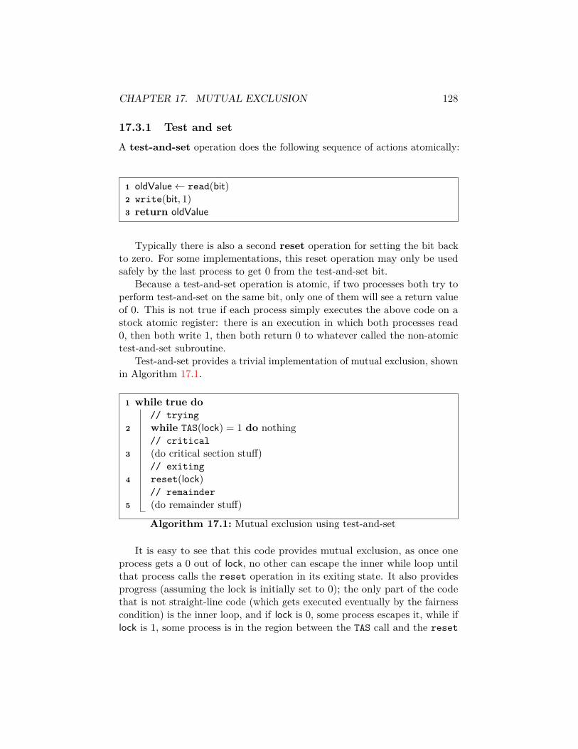
CHAPTER 17. MUTUAL EXCLUSION 128

17.3.1 Test and set

A test-and-set operation does the following sequence of actions atomically:

1 oldValue← read(bit)2 write(bit, 1)3 return oldValue

Typically there is also a second reset operation for setting the bit backto zero. For some implementations, this reset operation may only be usedsafely by the last process to get 0 from the test-and-set bit.

Because a test-and-set operation is atomic, if two processes both try toperform test-and-set on the same bit, only one of them will see a return valueof 0. This is not true if each process simply executes the above code on astock atomic register: there is an execution in which both processes read0, then both write 1, then both return 0 to whatever called the non-atomictest-and-set subroutine.

Test-and-set provides a trivial implementation of mutual exclusion, shownin Algorithm 17.1.

1 while true do// trying

2 while TAS(lock) = 1 do nothing// critical

3 (do critical section stuff)// exiting

4 reset(lock)// remainder

5 (do remainder stuff)

Algorithm 17.1: Mutual exclusion using test-and-set

It is easy to see that this code provides mutual exclusion, as once oneprocess gets a 0 out of lock, no other can escape the inner while loop untilthat process calls the reset operation in its exiting state. It also providesprogress (assuming the lock is initially set to 0); the only part of the codethat is not straight-line code (which gets executed eventually by the fairnesscondition) is the inner loop, and if lock is 0, some process escapes it, while iflock is 1, some process is in the region between the TAS call and the reset

CHAPTER 17. MUTUAL EXCLUSION 129

call, and so it eventually gets to reset and lets the next process in (or itself,if it is very fast).

The algorithm does not provide lockout-freedom: nothing prevents asingle fast process from scooping up the lock bit every time it goes throughthe outer loop, while the other processes ineffectually grab at it just after itis taken away. Lockout-freedom requires a more sophisticated turn-takingstrategy.

17.3.2 A lockout-free algorithm using an atomic queue

Basic idea: In the trying phase, each process enqueues itself on the end of ashared queue (assumed to be an atomic operation). When a process comesto the head of the queue, it enters the critical section, and when exiting itdequeues itself. So the code would look something like Algorithm 17.2.

Note that this requires a queue that supports a head operation. Not allimplementations of queues have this property.

1 while true do// trying

2 enq(Q,myId)3 while head(Q) 6= myId do nothing

// critical4 (do critical section stuff)

// exiting5 deq(Q)

// remainder6 (do remainder stuff)

Algorithm 17.2: Mutual exclusion using a queue

Here the proof of mutual exclusion is that only the process whose id is atthe head of the queue can enter its critical section. Formally, we maintain aninvariant that any process whose program counter is between the inner whileloop and the call to deq(Q) must be at the head of the queue; this invariantis easy to show because a process can’t leave the while loop unless the testfails (i.e., it is already at the head of the queue), no enq operation changesthe head value (if the queue is nonempty), and the deq operation (whichdoes change the head value) can only be executed by a process already atthe head (from the invariant).

Deadlock-freedom follows from proving a similar invariant that every

CHAPTER 17. MUTUAL EXCLUSION 130

element of the queue is the id of some process in the trying, critical, orexiting states, so eventually the process at the head of the queue passes theinner loop, executes its critical section, and dequeues its id.

Lockout-freedom follows from the fact that once a process is at positionk in the queue, every execution of a critical section reduces its positionby 1; when it reaches the front of the queue (after some finite number ofcritical sections), it gets the critical section itself. Alternatively, we can arguelockout-freedom by showing bounded bypass: once I am in the queue, noprocess can execute two critical sections before I do, because once it leavesits first critical section, it enqueues behind me.

17.3.2.1 Reducing space complexity

Following [AW04, §4.3.2], we can give an implementation of this algorithmusing a single read-modify-write (RMW) register instead of a queue; thisdrastically reduces the (shared) space needed by the algorithm. The reasonthis works is because we don’t really need to keep track of the position ofeach process in the queue itself; instead, we can hand out numerical ticketsto each process and have the process take responsibility for rememberingwhere its place in line is.

The RMW register has two fields, first and last, both initially 0. In-crementing last simulates an enqueue, while incrementing first simulates adequeue. The trick is that instead of testing if it is at the head of the queue,a process simply remembers the value of the last field when it “enqueued”itself, and waits for the first field to equal it.

Algorithm 17.3 shows the code from Algorithm 17.2 rewritten to use thistechnique. The way to read the RMW operations is that the first argumentspecifies the variable to update and the second specifies an expression forcomputing the new value. Each RMW operation returns the old state of theobject, before the update.

17.4 Mutual exclusion using only atomic registersWhile mutual exclusion is easier using powerful primitives, we can also solvethe problem using only registers.

17.4.1 Peterson’s algorithm

Algorithm 17.4 shows Peterson’s lockout-free mutual exclusion protocol fortwo processes p0 and p1 [Pet81] (see also [AW04, §4.4.2] or [Lyn96, §10.5.1]).

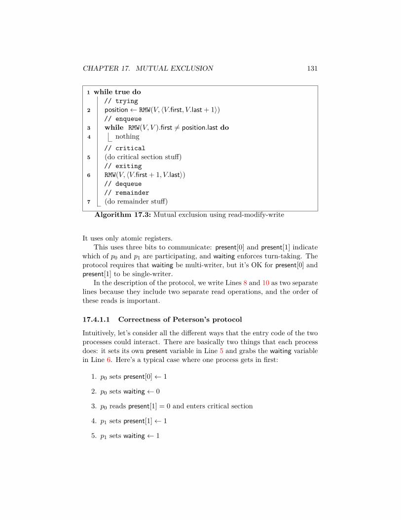
CHAPTER 17. MUTUAL EXCLUSION 131

1 while true do// trying

2 position← RMW(V, 〈V.first, V.last + 1〉)// enqueue

3 while RMW(V, V ).first 6= position.last do4 nothing

// critical5 (do critical section stuff)

// exiting6 RMW(V, 〈V.first + 1, V.last〉)

// dequeue// remainder

7 (do remainder stuff)

Algorithm 17.3: Mutual exclusion using read-modify-write

It uses only atomic registers.This uses three bits to communicate: present[0] and present[1] indicate

which of p0 and p1 are participating, and waiting enforces turn-taking. Theprotocol requires that waiting be multi-writer, but it’s OK for present[0] andpresent[1] to be single-writer.

In the description of the protocol, we write Lines 8 and 10 as two separatelines because they include two separate read operations, and the order ofthese reads is important.

17.4.1.1 Correctness of Peterson’s protocol

Intuitively, let’s consider all the different ways that the entry code of the twoprocesses could interact. There are basically two things that each processdoes: it sets its own present variable in Line 5 and grabs the waiting variablein Line 6. Here’s a typical case where one process gets in first:

1. p0 sets present[0]← 1

2. p0 sets waiting← 0

3. p0 reads present[1] = 0 and enters critical section

4. p1 sets present[1]← 1

5. p1 sets waiting← 1

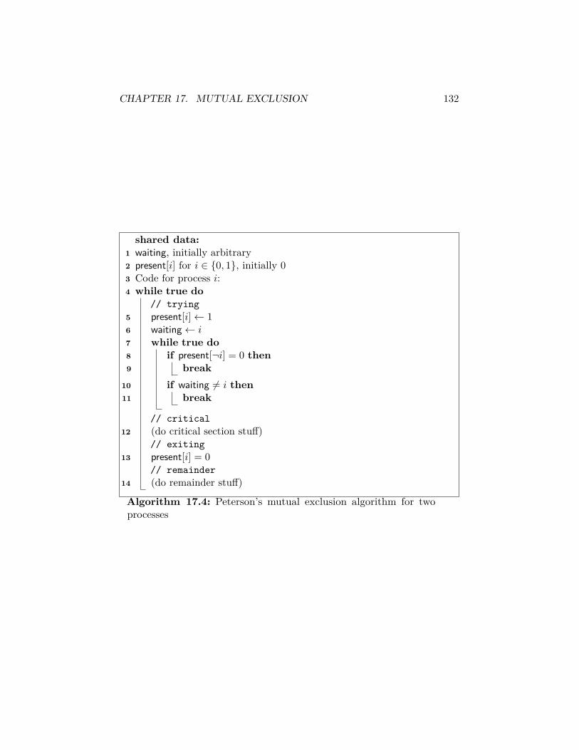
CHAPTER 17. MUTUAL EXCLUSION 132

shared data:1 waiting, initially arbitrary2 present[i] for i ∈ 0, 1, initially 03 Code for process i:4 while true do

// trying5 present[i]← 16 waiting← i7 while true do8 if present[¬i] = 0 then9 break

10 if waiting 6= i then11 break

// critical12 (do critical section stuff)

// exiting13 present[i] = 0

// remainder14 (do remainder stuff)

Algorithm 17.4: Peterson’s mutual exclusion algorithm for twoprocesses

CHAPTER 17. MUTUAL EXCLUSION 133

6. p1 reads present[0] = 1 and waiting = 1 and loops

7. p0 sets present[0]← 0

8. p1 reads present[0] = 0 and enters critical section

The idea is that if I see a 0 in your present variable, I know that youaren’t playing, and can just go in.

Here’s a more interleaved execution where the waiting variable decidesthe winner:

1. p0 sets present[0]← 1

2. p0 sets waiting← 0

3. p1 sets present[1]← 1

4. p1 sets waiting← 1

5. p0 reads present[1] = 1

6. p1 reads present[0] = 1

7. p0 reads waiting = 1 and enters critical section

8. p1 reads present[0] = 1 and waiting = 1 and loops

9. p0 sets present[0]← 0

10. p1 reads present[0] = 0 and enters critical section

Note that it’s the process that set the waiting variable last (and thus seesits own value) that stalls. This is necessary because the earlier process mightlong since have entered the critical section.

Sadly, examples are not proofs, so to show that this works in general,we need to formally verify each of mutual exclusion and lockout-freedom.Mutual exclusion is a safety property, so we expect to prove it using invariants.The proof in [Lyn96] is based on translating the pseudocode directly intoautomata (including explicit program counter variables); we’ll do essentiallythe same proof but without doing the full translation to automata. Below,we write that pi is at line k if it the operation in line k is enabled but hasnot occurred yet.

Lemma 17.4.1. If present[i] = 0, then pi is at Line 5 or 14.

CHAPTER 17. MUTUAL EXCLUSION 134

Proof. Immediate from the code.

Lemma 17.4.2. If pi is at Line 12, and p¬i is at Line 8, 10, or 12, thenwaiting = ¬i.

Proof. We’ll do the case i = 0; the other case is symmetric. The proof is byinduction on the schedule. We need to check that any event that makes theleft-hand side of the invariant true or the right-hand side false also makesthe whole invariant true. The relevant events are:

• Transitions by p0 from Line 8 to Line 12. These occur only if present[1] =0, implying p1 is at Line Line 5 or 14 by Lemma 17.4.1. In this casethe second part of the left-hand side is false.

• Transitions by p0 from Line 10 to Line 12. These occur only if waiting 6=0, so the right-hand side is true.

• Transitions by p1 from Line 6 to Line 8. These set waiting to 1, makingthe right-hand side true.

• Transitions that set waiting to 0. These are transitions by p0 fromLine 6 to Line 10, making the left-hand side false.

We can now read mutual exclusion directly off of Lemma 17.4.2: ifboth p0 and p1 are at Line 12, then we get waiting = 1 and waiting = 0, acontradiction.

To show progress, observe that the only place where both processes canget stuck forever is in the loop at Lines 8 and 10. But then waiting isn’tchanging, and so some process i reads waiting = ¬i and leaves. To showlockout-freedom, observe that if p0 is stuck in the loop while p1 enters thecritical section, then after p1 leaves it sets present[1] to 0 in Line 13 (whichlets p0 in if p0 reads present[1] in time), but even if it then sets present[1]back to 1 in Line 5, it still sets waiting to 1 in Line 6, which lets p0 intothe critical section. With some more tinkering this argument shows that p1enters the critical section at most twice while p0 is in the trying state, giving2-bounded bypass; see [Lyn96, Lemma 10.12]. With even more tinkering weget a constant time bound on the waiting time for process i to enter thecritical section, assuming the other process never spends more than O(1)time inside the critical section.

CHAPTER 17. MUTUAL EXCLUSION 135

17.4.1.2 Generalization to n processes

(See also [AW04, §4.4.3].)The easiest way to generalize Peterson’s two-process algorithm to n

processes is to organize a tournament in the form of log-depth binary tree;this method was invented by Peterson and Fischer [PF77]. At each nodeof the tree, the roles of the two processes are taken by the winners of thesubtrees, i.e., the processes who have entered their critical sections in thetwo-process algorithms corresponding to the child nodes. The winner ofthe tournament as a whole enters the real critical section, and afterwardswalks back down the tree unlocking all the nodes it won in reverse order.It’s easy to see that this satisfies mutual exclusion, and not much harderto show that it satisfies lockout-freedom—in the latter case, the essentialidea is that if a winner at some node reaches the root infinitely often, thenlockout-freedom at that node means that a winner of each child node reachesthe root infinitely often.

The most natural way to implement the nodes is to have present[0] andpresent[1] at each node be multi-writer variables that can be written to byany process in the appropriate subtree. Because the present variables don’tdo much, we can also implement them as the OR of many single-writervariables (this is what is done in [Lyn96, §10.5.3]), but there is no immediatepayoff to doing this since the waiting variables are still multi-writer.

Nice properties of this algorithm are that it uses only bits and that it’svery fast: O(logn) time in the absence of contention.

17.4.2 Fast mutual exclusion

With a bit of extra work, we can reduce the no-contention cost of mutualexclusion to O(1), while keeping whatever performance we previously hadin the high-contention case. The trick (due to Lamport [Lam87]) is to putan object at the entrance to the protocol that diverts a solo process onto a“fast path” that lets it bypass the n-process mutex that everybody else endsup on.

Our presentation mostly follows [AW04][§4.4.5], which uses the splitterabstraction of Moir and Anderson [MA95] to separate out the mechanismfor diverting a lone process.2 Code for a splitter is given in Algorithm 17.5.

A splitter assigns to each processes that arrives at it the value right, down,or stop. The useful properties of splitters are that if at least one process

2Moir and Anderson call these things one-time building blocks, but the namesplitter has become standard in subsequent work.

CHAPTER 17. MUTUAL EXCLUSION 136

shared data:1 atomic register race, big enough to hold an id, initially ⊥2 atomic register door, big enough to hold a bit, initially open3 procedure splitter(id)4 race← id5 if door = closed then6 return right7 door← closed8 if race = id then9 return stop

10 else11 return down

Algorithm 17.5: Implementation of a splitter

arrives at a splitter, then (a) at least one process returns right or stop; and(b) at least one process returns down or stop; (c) at most one process returnsstop; and (d) any process that runs by itself returns stop. The first twoproperties will be useful when we consider the problem of renaming inChapter 24; we will prove them there. The last two properties are what wewant for mutual exclusion.

The names of the variables race and door follow the presentation in[AW04, §4.4.5]; Moir and Anderson [MA95], following Lamport [Lam87],call these X and Y . As in [MA95], we separate out the right and downoutcomes—even though they are equivalent for mutex—because we will needthem later for other applications.

The intuition behind Algorithm 17.5 is that setting door to closed closesthe door to new entrants, and the last entrant to write its id to race wins(it’s a slow race), assuming nobody else writes race and messes things up.The added cost of the splitter is always O(1), since there are no loops.

To reset the splitter, write open to door. This allows new processes toenter the splitter and possibly return stop.

Lemma 17.4.3. After each time that door is set to open, at most one processrunning Algorithm 17.5 returns stop.

Proof. To simplify the argument, we assume that each process calls splitterat most once.

Let t be some time at which door is set to open (−∞ in the case of theinitial value). Let St be the set of processes that read open from door after

CHAPTER 17. MUTUAL EXCLUSION 137

time t and before the next time at which some process writes closed to door,and that later return stop by reaching Line 9.

Then every process in St reads door before any process in St writes door.It follows that every process in St writes race before any process in St readsrace. If some process p is not the last process in St to write race, it will notsee its own id, and will not return stop. But only one process can be the lastprocess in St to write race.3

Lemma 17.4.4. If a process runs Algorithm 17.5 by itself starting from aconfiguration in which door = open, it returns stop.

Proof. Follows from examining a solo execution: the process sets race to id,reads open from door, then reads id from race. This causes it to return stopas claimed.

To turn this into an n-process mutex algorithm, we use the splitter toseparate out at most one process (the one that gets stop) onto a fast paththat bypasses the slow path taken by the rest of the processes. The slow-path process first fight among themselves to get through an n-process mutex;the winner then fights in a 2-process mutex with the process (if any) on thefast path.

Releasing the mutex is the reverse of acquiring it. If I followed the fastpath, I release the 2-process mutex first then reset the splitter. If I followedthe slow path, I release the 2-process mutex first then the n-process mutex.This gives mutual exclusion with O(1) cost for any process that arrives beforethere is any contention (O(1) for the splitter plus O(1) for the 2-processmutex).

A complication is that if nobody wins the splitter, there is no fast-pathprocess to reset it. If we don’t want to accept that the fast path just breaksforever in this case, we have to include a mechanism for a slow-path processto reset the splitter if it can be assured that there is no fast-path processleft in the system. The simplest way to do this is to have each process marka bit in an array to show it is present, and have each slow-path process,while still holding all the mutexes, check on its way out if the door bit is setand no processes claim to be present. If it sees all zeros (except for itself)after seeing door = closed, it can safely conclude that there is no fast-pathprocess and reset the splitter itself. The argument then is that the lastslow-path process to leave will do this, re-enabling the fast path once there is

3It’s worth noting that this last process still might not return stop, because some laterprocess—not in St—might overwrite race. This can happen even if nobody ever resets thesplitter.

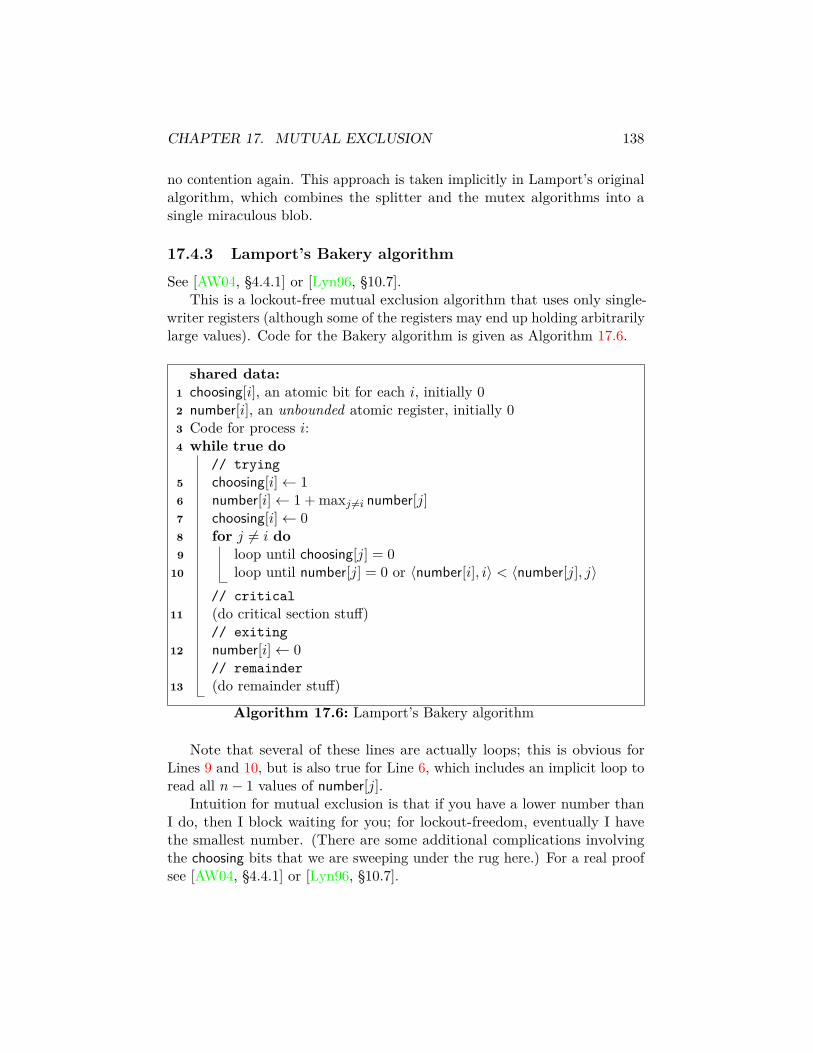
CHAPTER 17. MUTUAL EXCLUSION 138

no contention again. This approach is taken implicitly in Lamport’s originalalgorithm, which combines the splitter and the mutex algorithms into asingle miraculous blob.

17.4.3 Lamport’s Bakery algorithm

See [AW04, §4.4.1] or [Lyn96, §10.7].This is a lockout-free mutual exclusion algorithm that uses only single-

writer registers (although some of the registers may end up holding arbitrarilylarge values). Code for the Bakery algorithm is given as Algorithm 17.6.

shared data:1 choosing[i], an atomic bit for each i, initially 02 number[i], an unbounded atomic register, initially 03 Code for process i:4 while true do

// trying5 choosing[i]← 16 number[i]← 1 + maxj 6=i number[j]7 choosing[i]← 08 for j 6= i do9 loop until choosing[j] = 0

10 loop until number[j] = 0 or 〈number[i], i〉 < 〈number[j], j〉// critical

11 (do critical section stuff)// exiting

12 number[i]← 0// remainder

13 (do remainder stuff)

Algorithm 17.6: Lamport’s Bakery algorithm

Note that several of these lines are actually loops; this is obvious forLines 9 and 10, but is also true for Line 6, which includes an implicit loop toread all n− 1 values of number[j].

Intuition for mutual exclusion is that if you have a lower number thanI do, then I block waiting for you; for lockout-freedom, eventually I havethe smallest number. (There are some additional complications involvingthe choosing bits that we are sweeping under the rug here.) For a real proofsee [AW04, §4.4.1] or [Lyn96, §10.7].

CHAPTER 17. MUTUAL EXCLUSION 139

Selling point is a strong near-FIFO guarantee and the use of only single-writer registers (which need not even be atomic—it’s enough that they returncorrect values when no write is in progress). Weak point is unboundedregisters.

17.4.4 Lower bound on the number of registers

There is a famous result due to Burns and Lynch [BL93] that any mutualexclusion protocol using only read/write registers requires at least n ofthem. Details are in [Lyn96, §10.8]. A slightly different version of theargument is given in [AW04, §4.4.4]. The proof is another nice example of anindistinguishability proof, where we use the fact that if a group of processescan’t tell the difference between two executions, they behave the same inboth.

Assumptions: We have a protocol that guarantees mutual exclusion andprogress. Our base objects are all atomic registers.

Key idea: In order for some process p to enter the critical section, it hasto do at least one write to let the other processes know it is doing so. Ifnot, they can’t tell if p ever showed up at all, so eventually either some p′will enter the critical section and violate mutual exclusion or (in the no-pexecution) nobody enters the critical section and we violate progress. Nowsuppose we can park a process pi on each register ri with a pending write toi; in this case we say that pi covers ri. If every register is so covered, wecan let p go ahead and do whatever writes it likes and then deliver all thecovering writes at once, wiping out anything p did. Now the other processesagain don’t know if p exists or not. So we can say something stronger: beforesome process p can enter a critical section, it has to write to an uncoveredregister.

The hard part is showing that we can cover all the registers withoutletting p know that there are other processes waiting—if p can see that otherprocesses are waiting, it can just sit back and wait for them to go throughthe critical section and make progress that way. So our goal is to producestates in which (a) processes p1 . . . , pk (for some k) between them cover kregisters, and (b) the resulting configuration is indistinguishable from an idleconfiguration to pk+1 . . . pn, where an idle configuration is one in whichevery process is in its remainder section.Lemma 17.4.5. Starting from any idle configuration C, there exists an exe-cution in which only processes p1 . . . pk take steps that leads to a configurationC ′ such that (a) C ′ is indistinguishable by any of pk+1 . . . pn from some idleconfiguration C ′′ and (b) k distinct registers are covered by p1 . . . pk in C ′.

CHAPTER 17. MUTUAL EXCLUSION 140

Proof. The proof is by induction on k. For k = 0, let C ′′ = C ′ = C.For larger k, the essential idea is that starting from C, we first run

to a configuration C1 where p1 . . . pk−1 cover k − 1 registers and C1 isindistinguishable from an idle configuration by the remaining processes, andthen run pk until it covers one more register. If we let p1 . . . pk−1 go, theyoverwrite anything pk wrote. Unfortunately, they may not come back tocovering the same registers as before if we rerun the induction hypothesis(and in particular might cover the same register that pk does). So we haveto look for a particular configuration C1 that not only covers k − 1 registersbut also has an extension that covers the same k − 1 registers.

Here’s how we find it: Start in C. Run the induction hypothesis to getC1; here there is a set W1 of k− 1 registers covered in C1. Now let processesp1 through pk−1 do their pending writes, then each enter the critical section,leave it, and finish, and rerun the induction hypothesis to get to a state C2,indistinguishable from an idle configuration by pk and up, in which k − 1registers in W2 are covered. Repeat to get sets W3, W4, etc. Since thissequence is unbounded, and there are only

( rk−1)distinct sets of registers to

cover (where r is the number of registers), eventually we have Wi = Wj forsome i 6= j. The configurations Ci and Cj are now our desired configurationscovering the same k − 1 registers.

Now that we have Ci and Cj , we run until we get to Ci. We now run pkuntil it is about to write some register not covered by Ci (it must do so, orotherwise we can wipe out all of its writes while it’s in the critical section andthen go on to violate mutual exclusion). Then we let the rest of p1 throughpk−1 do all their writes (which immediately destroys any evidence that pkran at all) and run the execution that gets them to Cj . We now have k − 1registers covered by p1 through pk−1 and a k-th register covered by pk, in aconfiguration that is indistinguishable from idle: this proves the inductionstep.

The final result follows by the fact that when k = n we cover n registers;this implies that there are n registers to cover.

It’s worth noting that the execution constructed in this proof might bevery, very long. It’s not clear what happens if we consider executions in which,say, the critical section is only entered a polynomial number of times. If weare willing to accept a small probability of failure over polynomially-manyentries, there is a randomized mutex that runs in O(logn) space [AHTW18].

CHAPTER 17. MUTUAL EXCLUSION 141

17.5 RMR complexityIt’s not hard to see that we can’t build a shared-memory mutex withoutbusy-waiting: any process that is waiting can’t detect that the critical sectionis safe to enter without reading a register, but if that register tells it that itshould keep waiting, it is back where it started and has to read it again. Thismakes our standard step-counting complexity measures useless for describethe worst-case complexity of a mutual exclusion algorithm.

However, the same argument that suggests we can ignore local computa-tion in a message-passing model suggests that we can ignore local operationson registers in a shared-memory model. Real multiprocessors have memoryhierarchies where memory that is close to the CPU (or one of the CPUs)is generally much faster than memory that is more distant. This suggestscharging only for remote memory references, or RMRs, where eachregister is local to one of the processes and only operations on non-localregisters are expensive. This has the advantage of more accurately modelingreal costs [MCS91, And90], and allowing us to build busy-waiting mutualexclusion algorithms with costs we can actually analyze.

As usual, there is a bit of a divergence here between theory and practice.Practically, we are interested in algorithms with good real-time performance,and RMR complexity becomes a heuristic for choosing how to assign memorylocations. This gives rise to very efficient mutual exclusion algorithms forreal machines, of which the most widely used is the beautiful MCS algorithmof Mellor-Crummey and Scott [MCS91]. Theoretically, we are interested inthe question of how efficiently we can solve mutual exclusion in our formalmodel, and RMR complexity becomes just another complexity measure, onethat happens to allow busy-waiting on local variables.

17.5.1 Cache-coherence vs. distributed shared memory

The basic idea of RMR complexity is that a process doesn’t pay for operationson local registers. But what determines which operations are local?

In the cache-coherent model (CC for short), once a process reads aregister it retains a local copy as long as nobody updates it. So if I do asequence of read operations with no intervening operations by other processes,I may pay an RMR for the first one (if my cache is out of date), but the restare free. The assumption is that each process can cache registers, and thereis some cache-coherence protocol that guarantees that all the caches stay upto date. We may or may not pay RMRs for write operations or other readoperations, depending on the details of the cache-coherence protocol, but for

CHAPTER 17. MUTUAL EXCLUSION 142

upper bounds it is safest to assume that we do.In the distributed shared memory model (DSM), each register is

assigned permanently to a single process. Other processes can read or writethe register, but only the owner gets to do so without paying an RMR. Herememory locations are nailed down to specific processes.

In general, we expect the cache-coherent model to be cheaper than thedistributed shared-memory model, if we ignore constant factors. The reasonis that if we run a DSM algorithm in a CC model, then the process p towhich a register r is assigned incurs an RMR only if some other processq accesses p since p’s last access. But then we can amortize p’s RMR bycharging q double. Since q incurs an RMR in the CC model, this tells us thatwe pay at most twice as many RMRs in DSM as in CC for any algorithm.

The converse is not true: there are (mildly exotic) problems for which itis known that CC algorithms are asymptotically more efficient than DSMalgorithms [Gol11, DH04].

17.5.2 RMR complexity of Peterson’s algorithm

As a warm-up, let’s look at the RMR complexity of Peterson’s two-processmutual exclusion algorithm (Algorithm 17.4). Acquiring the mutex requiresgoing through mostly straight-line code, except for the loop that testspresent[¬i] and waiting.

In the DSM model, spinning on present[¬i] is not a problem (we canmake it a local variable of process i). But waiting is trouble. Whicheverprocess we don’t assign it to will pay an RMR every time it looks at it. SoPeterson’s algorithm behaves badly by the RMR measure in this model.

Things are better in the CC model. Now process i may pay RMRs for itsfirst reads of present[¬i] and waiting, but any subsequent reads are free unlessprocess ¬i changes one of them. But any change to either of the variablescauses process i to leave the loop. It follows that process i pays at most 3RMRs to get through the busy-waiting loop, giving an RMR complexity ofO(1).

RMR complexities for parts of a protocol that access different registersadd just like step complexities, so the Peterson-Fischer tree constructiondescribed in §17.4.1.2 works here too. The result is O(logn) RMRs percritical section access, but only in the CC model.

CHAPTER 17. MUTUAL EXCLUSION 143

17.5.3 Mutual exclusion in the DSM model

Yang and Anderson [YA95] give a mutual exclusion algorithm for the DSMmodel that requires Θ(logn) RMRs to reach the critical section. This is nowknown to be optimal for deterministic algorithms [AHW08]. The core of thealgorithm is a 2-process mutex similar to Peterson’s, with some tweaks sothat each process spins only on its own registers. Pseudocode is given inAlgorithm 17.7; this is adapted from [YA95, Figure 1].

1 C[side(i)]← i2 T ← i3 P [i]← 04 rival← C[¬side(i)]5 if rival 6= ⊥ and T = i then6 if P [rival] = 0 then7 P [rival] = 18 while P [i] = 0 do spin9 if T = i then

10 while P [i] ≤ 1 do spin

// critical section goes here11 C[side(i)]← ⊥12 rival← T13 if rival 6= i then14 P [rival]← 2

Algorithm 17.7: Yang-Anderson mutex for two processes

The algorithm is designed to be used in a tree construction where aprocess with id in the range 1 . . . n/2 first fights with all other processesin this range, and similarly for processes in the range n/2 + 1 . . . n. Thefunction side(i) is 0 for the first group of processes and 1 for the second.The variables C[0] and C[1] are used to record which process is the winnerfor each side, and also take the place of the present variables in Peterson’salgorithm. Each process has its own variable P [i] that it spins on whenblocked; this variable is initially 0 and ranges over 0, 1, 2; this is used tosignal a process that it is safe to proceed, and tests on P substitute for testson the non-local variables in Peterson’s algorithm. Finally, the variable T isused (like waiting in Peterson’s algorithm) to break ties: when T = i, it’s i’sturn to wait.

Initially, C[0] = C[1] = ⊥ and P [i] = 0 for all i.

CHAPTER 17. MUTUAL EXCLUSION 144

When I want to enter my critical section, I first set C[side(i)] so you canfind me; this also has the same effect as setting present[side(i)] in Peterson’salgorithm. I then point T to myself and look for you. I’ll block if I seeC[¬side(i)] = 1 and T = i. This can occur in two ways: one is that I reallywrite T after you did, but the other is that you only wrote C[¬side(i)] buthaven’t written T yet. In the latter case, you will signal to me that T mayhave changed by setting P [i] to 1. I have to check T again (because maybe Ireally did write T later), and if it is still i, then I know that you are ahead ofme and will succeed in entering your critical section. In this case I can safelyspin on P [i] waiting for it to become 2, which signals that you have left.

There is a proof that this actually works in [YA95], but it’s 27 pagesof very meticulously-demonstrated invariants (in fairness, this includes theentire algorithm, including the tree parts that we omitted here). For intuition,this is not much more helpful than having a program mechanically check allthe transitions, since the algorithm for two processes is effectively finite-stateif we ignore the issue with different processes i jumping into the role ofside(i).

A slightly less rigorous but more human-accessible proof would be analo-gous to the proof of Peterson’s algorithm. We need to show two things: first,that no two processes ever both enter the critical section, and second, thatno process gets stuck.

For the first part, consider two processes i and j, where side(i) = 0 andside(j) = 1. We can’t have both i and j skip the loops, because whicheverone writes T last sees itself in T . Suppose that this is process i and thatj skips the loops. Then T = i and P [i] = 0 as long as j is in the criticalsection, so i blocks. Alternatively, suppose i writes T last but does so afterj first reads T . Now i and j both enter the loops. But again i sees T = i onits second test and blocks on the second loop until j sets P [i] to 2, whichdoesn’t happen until after j finishes its critical section.

Now let us show that i doesn’t get stuck. Again we’ll assume that i wroteT second.

If j skips the loops, then j sets P [i] = 2 on its way out as long as T = i;this falsifies both loop tests. If this happens after i first sets P [i] to 0, onlyi can set P [i] back to 0, so i escapes its first loop, and any j′ that entersfrom the 1 side will see P [i] = 2 before attempting to set P [i] to 1, so P [i]remains at 2 until i comes back around again. If j sets P [i] to 2 before i setsP [i] to 0 (or doesn’t set it at all because T = j, then C[side(j)] is set to ⊥before i reads it, so i skips the loops.

If j doesn’t skip the loops, then P [i] and P [j] are both set to 1 after iand j enter the loopy part. Because j waits for P [j] 6= 0, when it looks at

CHAPTER 17. MUTUAL EXCLUSION 145

T the second time it will see T = i 6= j and will skip the second loop. Thiscauses it to eventually set P [i] to 2 or set C[side(j)] to ⊥ before i reads itas in the previous case, so again i eventually reaches its critical section.

Since the only operations inside a loop are on local variables, the algorithmhas O(1) RMR complexity. For the full tree this becomes O(logn).

17.5.4 Lower bounds

For deterministic algorithms, there is a lower bound due to Attiya, Hendler,and Woelfel [AHW08] that shows that any one-shot mutual exclusion algo-rithm for n processes incurs Ω(n logn) total RMRs in either the CC or DSMmodels (which implies that some single process incurs Ω(logn) RMRs). Thisis based on an earlier breakthrough lower bound of Fan and Lynch [FL06]that proved the same lower bound for the number of times a register changesstate. Both bounds are information-theoretic: a family of n! executionsis constructed containing all possible orders in which the processes enterthe critical section, and it is shown that each RMR or state change onlycontributes O(1) bits to choosing between them.

For randomized algorithms, Hendler and Woelfel [HW11] have an al-gorithm that uses O(logn/ log logn) expected RMRs against an adaptiveadversary, beating the deterministic lower bound. This is the best possiblefor an adaptive adversary, due to a matching lower bound of Giakkoupis andWoelfel [GW12b] that holds even for systems that provide compare-and-swapobjects.

For an oblivious adversary, an algorithm of Giakkoupis andWoelfel [GW14]achieves O(1) expected RMRs in the DSM model. With compare-and-swap,a more recent algorithm of Giakkoupis and Woelfel [GW17] gives O(1) ex-pected RMRs in the CC model. Curiously, there also exist linearizableO(1)-RMR implementations of CAS from registers in this model [GHHW12];however, it is not clear that these implementations can be combined with theGiakkoupis-Woelfel algorithm to give O(1) expected RMRs using registers,because variations in scheduling of randomized implementations may producesubtle conditioning that gives different behavior from actual atomic objectsin the context of a randomized algorithm [GHW11].

Chapter 18

The wait-free hierarchy

In a shared memory model, it may be possible to solve some problemsusing wait-free protocols, in which any process can finish the protocol in abounded number of steps, no matter what the other processes are doing (seeChapter 26 for more on this and some variants).

The wait-free hierarchy hrm classifies asynchronous shared-memoryobject types T by consensus number, where a type T has consensusnumber n if with objects of type T and atomic registers (all initialized toappropriate values1) it is possible to solve wait-free consensus (i.e., agreement,validity, wait-free termination) for n processes but not for n+ 1 processes.The consensus number of any type is at least 1, since 1-process consensusrequires no interaction, and may range up to ∞ for particularly powerfulobjects.

The general idea is that a type T with consensus number c can’t simulateat type T ′ with a higher consensus number c′, because then we could usethe simulation to convert a c′-process consensus protocol using T ′ into ac′-process consensus protocol using T . The converse claim, that objectswith the same or higher consensus numbers can simulate those with lowerones, is not necessarily true: even though n-process consensus can implementany object for n processes (see §18.2), it may be that for more than n

1The justification for assuming that the objects can be initialized to an arbitrary stateis a little tricky. The idea is that if we are trying to implement consensus from objects oftype T that are themselves implemented in terms of objects of type S, then it’s natural toassume that we initialize our simulated type-T objects to whatever states are convenient.Conversely, if we are using the ability of type-T objects to solve n-process consensus toshow that they can’t be implemented from type-S objects (which can’t solve n-processconsensus), then for both the type-T and type-S objects we want these claims to hold nomatter how they are initialized.

146

CHAPTER 18. THE WAIT-FREE HIERARCHY 147

processes there is some object that has consensus number n but that cannotbe implemented from an arbitrary n-consensus object.2

The wait-free hierarchy was suggested by work by Maurice Herlihy [Her91b]that classified many common (and some uncommon) shared-memory objectsby consensus number, and showed that an unbounded collection of objectswith consensus number n together with atomic registers gives a wait-freeimplementation of any object in an n-process system.

Various subsequent authors noticed that this did not give a robusthierarchy in the sense that combining two types of objects with consensusnumber n could solve wait-free consensus for larger n, and the hierarchyhrm was proposed by Prasad Jayanti [Jay97] as a way of classifying objectsthat might be robust: an object is at level n of the hrm hierarchy if havingunboundedly many objects plus unboundedly many registers solves n-processwait-free consensus but not (n+ 1)-process wait-free consensus.3

Whether or not the resulting hierarchy is in fact robust for arbitrarydeterministic objects is still open, but Ruppert [Rup00] subsequently showedthat it is robust for RMW registers and objects with a read operation thatreturns the current state, and there is a paper by Borowsky, Gafni, andAfek [BGA94] that sketches a proof based on a topological characterizationof computability4 that hrm is robust for deterministic objects that don’tdiscriminate between processes (unlike, say, single-writer registers). So forwell-behaved shared-memory objects (deterministic, symmetrically accessible,with read operations, etc.), consensus number appears to give a real classi-fication that allows us to say for example that any collection of read-writeregisters (consensus number 1), fetch-and-increments (2), test-and-set bits(2), and queues (2) is not enough to build a compare-and-swap (∞).5

Another useful result from the Borowsky-Gafni-Afek paper is that theconsensus number is not generally dependent on what assumptions we makeabout the initial state of the objects. Specifically, [BGA94, Lemma 3.2]states that as long as there is some sequence of operations that takes anobject from a fixed initial state to a desirable initial state for consensus, then

2The existence of such objects was eventually demonstrated by Afek, Ellen, andGafni [AEG16].

3The r in hrm stands for the registers, the m for having many objects of the given type.Jayanti [Jay97] also defines a hierarchy hr1 where you only get finitely many objects. Theh stands for “hierarchy,” or, more specifically, h(T ) stands for the level of the hierarchy atwhich T appears [Jay11].

4See Chapter 28.5Ruppert’s paper is particularly handy because it gives an algorithm for computing

the consensus number of the objects it considers. However, for infinite-state objects, thisrequires solving the halting problem (as previously shown by Jayanti and Toueg [JT92].

CHAPTER 18. THE WAIT-FREE HIERARCHY 148

we can safely assume that the object is in the desirable state. The core ideaof the proof is that each process can initialize its own copy of the objectand then announce that it is ready; each process will then participate in asequence of consensus protocols using the objects that they observe are ready,with the output of each protocol used as the input to the next. Because thefirst object Si to be announced as initialized will be visible to all processes,they will all do consensus using Si. Any subsequent protocols that may beused by only a subset of the processes will not change the common agreedoutput from the Si protocol.6

When considering multiple objects, the usual assumption is that objectsare combined by putting them next to each other. If we can combine twoobjects by constructing a single object with operations of both—which isessentially what happens when we apply different machine language instruc-tions to the same memory location—then the object with both operationsmay have a higher consensus number than the object with either opera-tion individually. This was observed by Ellen et al. [EGSZ16]. A simpleexample would be a register than supports increment (+1) and doubling(×2) operations. A register with only one of these operations is equivalentto a counter and has consensus number 1. But a register with both oper-ations has consensus number at least 2, since if it is initialized to 2, wecan tell which of the two operations went first by looking at the final value:3 = 2 + 1, 4 = 2× 2, 5 = (2× 2) + 1, 6 = (2 + 1)× 2.

We won’t attempt to do the robustness proofs of Borowsky et al. [BGA94]or Ruppert [Rup00]. Instead, we’ll concentrate on Herlihy’s original resultsand show that specific objects have specific consensus numbers when used inisolation. The procedure in each case will be to show an upper bound on theconsensus number using a variant of Fischer-Lynch-Paterson (made easierbecause we are wait-free and don’t have to worry about fairness) and thenshow a matching lower bound (for non-trivial upper bounds) by exhibitingan n-process consensus protocol for some n. Essentially everything below istaken from Herlihy’s paper [Her91b], so reading that may make more sensethan reading these notes.

18.1 Classification by consensus numberHere we show the position of various types in the wait-free hierarchy. Thequick description is shown in Table 18.1; more details (mostly adapted

6The result in the paper is stated for a consensus protocol that uses a single copy of theobject, but it generalizes in the obvious way to those that use multiple copies of the object.

CHAPTER 18. THE WAIT-FREE HIERARCHY 149

Consensusnumber

Definingcharacteristic

Examples

1 Read withinterferingno-returnRMW.

Registers, counters,generalized counters, max registers,atomic snapshots.

2 InterferingRMW; queue-like structures.

Test-and-set, fetch-and-add, queues,process-to-memory swap.

m m-process consensus objects.2m− 2 Atomic m-register write.∞ First write-like

operation wins.Queue with peek, fetch-and-cons,sticky bits, compare-and-swap,memory-to-memory swap, memory-to-memory copy.

Table 18.1: Position of various types in the wait-free hierarchy

from [Her91b]) are given below.

18.1.1 Level 1: atomic registers, counters, other interferingRMW registers that don’t return the old value

First observe that any type has consensus number at least 1, since 1-processconsensus is trivial.

We’ll argue that a large class of particularly weak objects has consensusnumber exactly 1, by running FLP with 2 processes. Recall from Chap-ter 11 that in the Fischer-Lynch-Paterson [FLP85] proof we classify statesas bivalent or univalent depending on whether both decision values are stillpossible, and that with at least one failure we can always start in a bivalentstate (this doesn’t depend on what objects we are using, since it dependsonly on having invisible inputs). Since the system is wait-free there is noconstraint on adversary scheduling, and so if any bivalent state has a bivalentsuccessor we can just do it. So to solve consensus we have to reach a bivalentconfiguration C that has only univalent successors, and in particular has a0-valent and a 1-valent successor produced by applying operations x and yof processes px and py.

Assuming objects don’t interact with each other behind the scenes, xand y must be operations of the same object. Otherwise Cxy = Cyx and we

CHAPTER 18. THE WAIT-FREE HIERARCHY 150

get a contradiction.Now let’s suppose we are looking at atomic registers, and consider cases:

• x and y are both reads, Then x and y commute: Cxy = Cyx, and weget a contradiction.

• x is a read and y is a write. Then py can’t tell the difference betweenCyx and Cxy, so running py to completion gives the same decisionvalue from both Cyx and Cxy, another contradiction.

• x and y are both writes. Now py can’t tell the difference between Cxyand Cy, so we get the same decision value for both, again contradictingthat Cx is 0-valent and Cy is 1-valent.

There’s a pattern to these cases that generalizes to other objects. Supposethat an object has a read operation that returns its state and one or moreread-modify-write operations that don’t return anything (perhaps we couldcall them “modify-write” operations). We’ll say that the MW operations areinterfering if, for any two operations x and y, either:

• x and y commute: Cxy = Cyx.

• One of x and y overwrites the other: Cxy = Cy or Cyx = Cx.

Then no pair of read or modify-write operations can get us out of abivalent state, because (a) reads commute; (b) for a read and MW, thenon-reader can’t tell which operation happened first; (c) and for any twoMW operations, either they commute or the overwriter can’t detect that thefirst operation happened. So any MW object with uninformative, interferingMW operations has consensus number 1.

For example, consider a counter that supports operations read, increment,decrement, and write: a write overwrites any other operation, and incrementsand decrements commute with each other, so the counter has consensusnumber 1. The same applies to a generalized counter that supports anatomic x← x+ a operation; as long as this operation doesn’t return the oldvalue, it still commutes with other atomic increments.

Max registers [AACH12], which have read operations that return thelargest value previously written, also have commutative updates, so they alsohave consensus number 1. This gives an example of an object not inventedat the time of Herlihy’s paper that is still covered by Herlihy’s argument.

CHAPTER 18. THE WAIT-FREE HIERARCHY 151

18.1.2 Level 2: interfering RMW objects that return the oldvalue, queues (without peek)

Suppose now that we have a RMW object that returns the old value, andsuppose that it is non-trivial in the sense that it has at least one RMWoperation where the embedded function f that determines the new value isnot the identity (otherwise RMW is just read). Then there is some value vsuch that f(v) 6= v. To solve two-process consensus, have each process pi firstwrite its preferred value to a register ri, then execute the non-trivial RMWoperation on the RMW object initialized to v. The first process to executeits operation sees v and decides its own value. The second process sees f(v)and decides the first process’s value (which it reads from the register). Itfollows that non-trivial RMW object has consensus number at least 2.

In many cases, this is all we get. Suppose that the operations of someRMW type T are non-interfering in a way analogous to the previous definition,where now we say that x and y commute if they leave the object in the samestate (regardless of what values are returned) and that y overwrites x if theobject is always in the same state after both x and xy (again regardlessof what is returned). The two processes px and py that carry out x and yknow what happened, but a third process pz doesn’t. So if we run pz tocompletion we get the same decision value after both Cx and Cy, whichmeans that Cx and Cy can’t be 0-valent and 1-valent. It follows that nocollection of RMW registers with interfering operations can solve 3-processconsensus, and thus all such objects have consensus number 2. Examplesof these objects include test-and-set bits, fetch-and-add registers, andswap registers that support an operation swap that writes a new value andreturns the previous value.

There are some other objects with consensus number 2 that don’t fit thispattern. Define a wait-free queue as an object with enqueue and dequeueoperations (like normal queues), where dequeue returns ⊥ if the queue isempty (instead of blocking). To solve 2-process consensus with a wait-freequeue, initialize the queue with a single value (it doesn’t matter what thevalue is). We can then treat the queue as a non-trivial RMW register wherea process wins if it successfully dequeues the initial value and loses if it getsempty.7

7But wait! What if the queue starts empty?This turns out to be a surprisingly annoying problem, and was one of the motivating

examples for hrm as opposed to Herlihy’s vaguer initial definition.With one empty queue and nothing else, Jayanti and Toueg [JT92, Theorem 7] show that

there is no solution to consensus for two processes. This is also true for stacks (Theorem 8

CHAPTER 18. THE WAIT-FREE HIERARCHY 152

However, enqueue operations are non-interfering: if px enqueues vx andpy enqueues vy, then any third process can detect which happened first;similarly we can distinguish enq(x)deq() from deq()enq(x). So to show wecan’t do three process consensus we do something sneakier: given a bivalentstate C with allegedly 0- and 1-valent successors Cenq(x) and Cenq(y),consider both Cenq(x)enq(y) and Cenq(y)enq(x) and run px until it doesa deq() (which it must, because otherwise it can’t tell what to decide) andthen stop it. Now run py until it also does a deq() and then stop it. We’venow destroyed the evidence of the split and poor hapless pz is stuck. In thecase of Cdeq()enq(x) and Cenq(x)deq() on a non-empty queue we can killthe initial dequeuer immediately and then kill whoever dequeues x or thevalue it replaced, and if the queue is empty only the dequeuer knows. Ineither case we reach indistinguishable states after killing only 2 witnesses,and the queue has consensus number at most 2.

Similar arguments work on stacks, deques, and so forth—these all haveconsensus number exactly 2.

18.1.3 Level ∞: objects where the first write wins

These are objects that can solve consensus for any number of processes. Hereare a bunch of level-∞ objects:

Queue with peek Has operations enq(x) and peek(), which returns thefirst value enqueued. (Maybe also deq(), but we don’t need it forconsensus). Protocol is to enqueue my input and then peek and returnthe first value in the queue.

Fetch-and-cons Returns old cdr and adds new car on to the head of a list.Use preceding protocol where peek() = tail(car :: cdr).

Sticky bit Has a write operation that has no effect unless register is in theinitial ⊥ state. Whether the write succeeds or fails, it returns nothing.The consensus protocol is to write my input and then return result ofa read.

Compare-and-swap Has CAS(old, new) operation that writes new only ifprevious value is old. Use it to build a sticky bit.

Load-linked/store-conditional Like compare-and-swap split into two op-erations. The operation reads a memory location and marks it. The

from the same paper). But adding a register (Theorem 9) lets you do it. A second emptyqueue also works.

CHAPTER 18. THE WAIT-FREE HIERARCHY 153

operation succeeds only if the location has not been changed since thepreceding load-linked by the same process. Can be used to build asticky bit.

Memory-to-memory swap Has swap(ri, rj) operation that atomicallyswaps contents of ri with rj , as well as the usual read and writeoperations for all registers. Use to implement fetch-and-cons. Alterna-tively, use two registers input[i] and victory[i] for each process i, wherevictory[i] is initialized to 0, and a single central register prize, initializedto 1. To execute consensus, write your input to input[i], then swapvictory[i] with prize. The winning value is obtained by scanning allthe victory registers for the one that contains a 1, then returning thecorresponding input value.)

Memory-to-memory copy Has a copy(ri, rj) operation that copies ri torj atomically. Use the same trick as for memory-to-memory swap,where a process copies prize to victory[i]. But now we have a processfollow up by writing 0 to prize. As soon as this happens, the victoryvalues are now fixed; take the leftmost 1 as the winner.8

Herlihy [Her91b] gives a slightly more complicated version of thisprocedure, where there is a separate prize[i] register for each i, andafter doing its copy a process writes 0 to all of the prize registers. Thisshows that memory-to-memory copy solves consensus for arbitrarilymany processes even if we insist that copy operations can never overlap.The same trick also works for memory-to-memory swap, since we cantreat a memory-to-memory swap as a memory-to-memory copy giventhat we don’t care what value it puts in the prize[i] register.

Bank accounts A bank account object stores a non-negative integer,and supports a read operation that returns the current value and awithdraw(k) operation that reduces the value by k, unless this wouldreduce the value below 0, in which case it has no effect.To solve (binary) consensus with a bank account, start it with 3, andhave each process with input b attempt to withdraw 3 − b from theaccount. After the first withdrawal, the object will hold either 0 or 1,and no further withdrawals will have any effect. So the bank accountacts exactly like a sticky bit where 3 represents ⊥.9

8Or use any other rule that all processes apply consistently.9If you have more money, you can extend this construction to any fixed set of values.

For example, to choose among values v in 0 . . .m− 1, start with 2m and have a process

CHAPTER 18. THE WAIT-FREE HIERARCHY 154

For many years, I assumed that this example demonstrated why cryp-tocurrencies all seem to use embedded consensus protocols of somesort. However, it turns out that there is a critical assumption neededfor this proof, which is that more than one process can spend from thesame account. Without this assumption, it has been shown by Guer-raoui et al. [GKM+19] that the consensus number of a single-spenderbank account is 1, and more generally that the consensus number of ak-spender bank account is exactly k.

18.1.4 Level 2m− 2: simultaneous m-register write

Here we have a (large) collection of atomic registers augmented by an m-register write operation that performs all the writes simultaneously. Theintuition for why this is helpful is that if p1 writes r1 and rshared while p2writes r2 and rshared then any process can look at the state of r1, r2 andrshared and tell which write happened first. Code for this procedure is givenin Algorithm 18.1; note that up to 4 reads may be necessary to determinethe winner because of timing issues.10

The workings of Algorithm 18.1 are straightforward:

• If the process reads r1 = r2 = ⊥, then we don’t care which went first,because the reader (or somebody else) already won.

• If the process reads r1 = 1 and then r2 = ⊥, then p1 went first.

• If the process reads r2 = 2 and then r1 = ⊥, then p2 went first. (Thisrequires at least one more read after checking the first case.)

• Otherwise the process saw r1 = 1 and r2 = 2. Now read rshared: if it’s1, p2 went first; if it’s 2, p1 went first.

Algorithm 18.1 requires 2-register writes, and will give us a protocol for 2processes (since the reader above has to participate somewhere to make thefirst case work). For m processes, we can do the same thing with m-registerwrites. We have a register rpq = rqp for each pair of distinct processes pand q, plus a register rpp for each p; this gives a total of

(m2)

+m = O(m2)

with input v subtract 2m− v.10The main issue is that processes can only read the registers one at a time. An

alternative to running Algorithm 18.1 is to use a double-collect snapshot (see §19.1) tosimulate reading all three registers at once. However, this might require as many as twelveread operations, since a process doing a snapshot has to re-read all three registers if any ofthem change.

CHAPTER 18. THE WAIT-FREE HIERARCHY 155

1 v1 ← r12 v2 ← r23 if v1 = v2 = ⊥ then4 return no winner5 if v1 = 1 and v2 = ⊥ then

// p1 went first6 return 1

// read r1 again7 v′1 ← r18 if v2 = 2 and v′1 = ⊥ then

// p2 went first9 return 2

// both p1 and p2 wrote10 if rshared = 1 then11 return 212 else13 return 1

Algorithm 18.1: Determining the winner of a race between 2-registerwrites. The assumption is that p1 and p2 each wrote their own idsto ri and rshared simultaneously. This code can be executed by anyprocess (including but not limited to p1 or p2) to determine which ofthese 2-register writes happened first.

CHAPTER 18. THE WAIT-FREE HIERARCHY 156

registers. All registers are initialized to ⊥. Process p then writes its initialpreference to some single-writer register prefp and then simultaneously writesp to rpq for all q (including rpp). It then attempts to figure out the firstwriter by applying the above test for each q to rpq (standing in for rshared),rpp (r1) and rqq (r2). If it won against all the other processes, it decides itsown value. If not, it repeats the test recursively for some p′ that beat it untilit finds a process that beat everybody, and returns its value. So m-registerwrites solve m-process wait-free consensus.

A further tweak gets 2m − 2: run two copies of an (m − 1)-processprotocol using separate arrays of registers to decide a winner for each group.Then add a second phase where processes contend across the groups. Thisinvolves each process p from group 1 writing the winning id for its groupsimultaneously into sp and spq for each q in the other group. To figure outwho won in the end, build a graph of all victories, where there is an edgefrom p to q if and only if p beat q in Phase 1 or p’s id was written before q’sid in Phase 2. The winner is the (unique) process with at least one outgoingedge and no incoming edges, which will be the process that won its owngroup (by writing first) and whose value was written first in Phase 2.

One thing to note about the second phase is that, unlike mutex, we can’tjust have the winners of the two groups fight each other, since this wouldnot give the wait-free property for non-winners. Instead, we have to allow anon-winner p to pick up the slack for a slow winner and fight on behalf ofthe entire group. This requires an m-process write operation to write sp andall spq at once.

18.1.4.1 Matching impossibility result

It might seem that the technique used to boost from m-process consensus to(2m−2)-process consensus could be repeated to get up to at least Θ(m2), butthis turns out not to be the case. The essential idea is to show that in orderto escape bivalence, we have to get to a configuration C where every processis about to do an m-register write leading to a univalent configuration (sincereads don’t help for the usual reasons, and normal writes can be simulatedby m-register writes with an extra m− 1 dummy registers), and then arguethat these writes can’t overlap too much. So suppose we are in such aconfiguration, and suppose that Cx is 0-valent and Cy is 1-valent, andwe also have many other operations z1 . . . zk that lead to univalent states.Following Herlihy [Her91b], we argue in two steps:

1. There is some register that is written to by x alone out of all the

CHAPTER 18. THE WAIT-FREE HIERARCHY 157

pending operations. Proof: Suppose not. Then the 0-valent configura-tion Cxyz1 . . . zk is indistinguishable from the 1-valent configurationCyz1 . . . zk by any process except px, and we’re in trouble.

2. There is some register that is written to by x and y but not by any ofthe zi. Proof:: Suppose not. The each register is written by at mostone of x and y, making it useless for telling which went first; or it isoverwritten by some zi, hiding the value that tells which went first.So Cxyz1 . . . zk is indistinguishable from Cyxz1 . . . zk for any processother than px and py, and we’re still in trouble.

Now suppose we have 2m− 1 processes. The first part says that each ofthe pending operations (x, y, all of the zi) writes to 1 single-writer registerand at least k two-writer registers where k is the number of processes leadingto a different univalent value. This gives k + 1 total registers simultaneouslywritten by this operation. Now observe that with 2m− 1 process, there issome set of m processes whose operations all lead to a b-valent state; sofor any process to get to a (¬b)-valent state, it must write m+ 1 registerssimultaneously. It follows that with only m simultaneous writes we can onlydo (2m− 2)-consensus.

18.1.5 Level m: m-process consensus objects

An m-process consensus object has a single consensus operation that,the first m times it is called, returns the input value in the first operation,and thereafter returns only ⊥. Clearly this solves m-process consensus. Toshow that it doesn’t solve (m+ 1)-process consensus even when augmentedwith registers, run a bivalent initial configuration to a configuration C whereany further operation yields a univalent state. By an argument similar tothe m-register write case, we can show that the pending operations in Cmust all be consensus operations on the same consensus object (anythingelse commutes or overwrites). Now run Cxyz1 . . . zk and Cyxz1 . . . zk, wherex and y lead to 0-valent and 1-valent states, and observe that pk can’tdistinguish the resulting configurations because all it got was ⊥. (Note: thisworks even if the consensus object isn’t in its initial state, since we knowthat before x or y the configuration is still bivalent.)

So the m-process consensus object has consensus number m. This showsthat hrm is nonempty at each level.

A natural question at this point is whether the inability of m-processconsensus objects to solve (m+1)-process consensus implies robustness of thehierarchy. One might consider the following argument: given any object at

CHAPTER 18. THE WAIT-FREE HIERARCHY 158

level m, we can simulate it with an m-process consensus object, and since wecan’t combine m-process consensus objects to boost the consensus number,we can’t combine any objects they can simulate either. The problem here isthat while m-process consensus objects can simulate any object in a systemwith m processes (see below), it may be that some objects can do more in asystem with m+ 1 objects while still not solving (m+ 1)-process consensus.A simple way to see this would be to imagine a variant of the m-processconsensus object that doesn’t fail completely after m operations; for example,it might return one of the first two inputs given to it instead of ⊥. Thisdoesn’t help with solving consensus, but it might (or might not) make it toopowerful to implement using standard m-process consensus objects.

18.2 Universality of consensusUniversality of consensus says that any type that can implement n-process consensus can, together with atomic registers, give a wait-free im-plementation of any object in a system with n processes. That consensusis universal was shown by Herlihy [Her91b] and Plotkin [Plo89]. Both ofthese papers spend a lot of effort on making sure that both the cost of eachoperation and the amount of space used is bounded. But if we ignore theseconstraints, the same result can be shown using a mechanism similar to thereplicated state machines of §12.3.

Here the processes repeatedly use consensus to decide between candidatehistories of the simulated object, and a process successfully completes anoperation when its operation (tagged to distinguish it from other similaroperations) appears in a winning history. A round structure avoids too muchconfusion.

Details are given in Algorithm 18.2.There are some subtleties to this algorithm. The first time that a process

calls consensus (on c[r]), it may supply a dummy input; the idea is that it isonly using the consensus object to obtain the agreed-upon history from around it missed. It’s safe to do this, because no process writes r to its roundregister until c[r] is complete, so the dummy input can’t be accidentallychosen as the correct value.

It’s not hard to see that whatever hr+1 is chosen in c[r+1] is an extensionof hr (it is constructed by appending operations to hr), and that all processesagree on it (by the agreement property of the consensus object c[r + 1]. Sothis gives us an increasing sequence of consistent histories. We also need toshow that these histories are linearizable. The obvious linearization is just

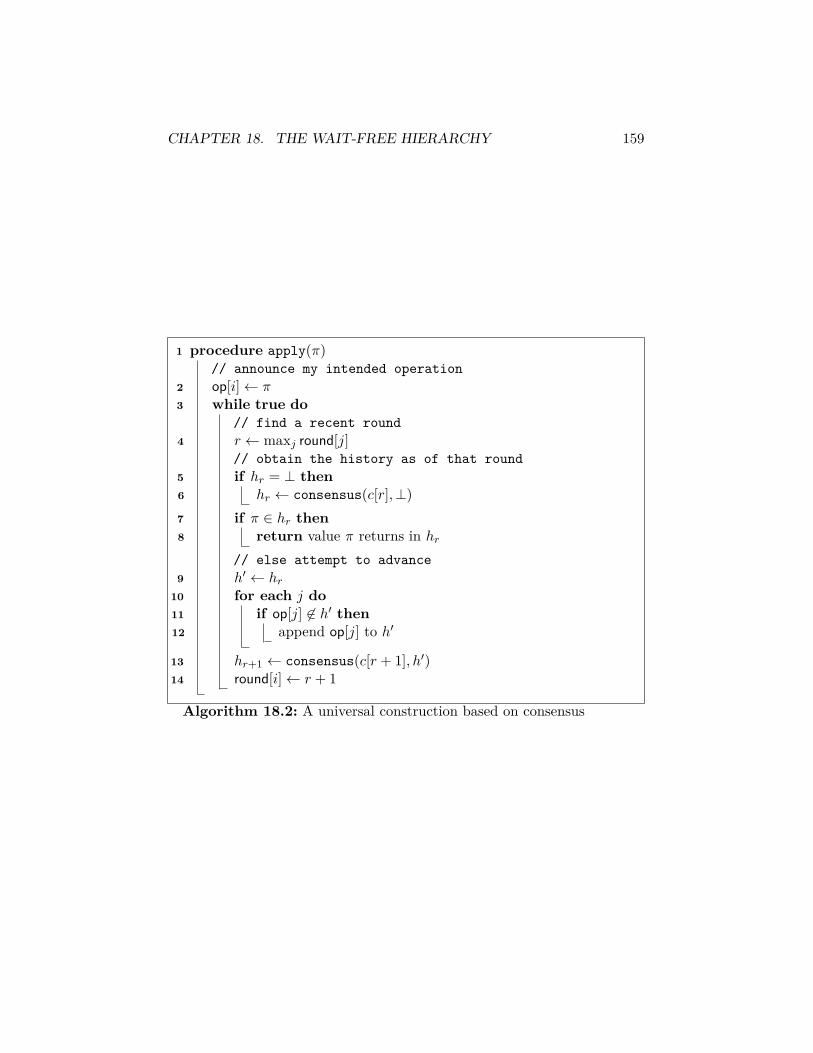
CHAPTER 18. THE WAIT-FREE HIERARCHY 159

1 procedure apply(π)// announce my intended operation

2 op[i]← π3 while true do

// find a recent round4 r ← maxj round[j]

// obtain the history as of that round5 if hr = ⊥ then6 hr ← consensus(c[r],⊥)7 if π ∈ hr then8 return value π returns in hr

// else attempt to advance9 h′ ← hr

10 for each j do11 if op[j] 6∈ h′ then12 append op[j] to h′

13 hr+1 ← consensus(c[r + 1], h′)14 round[i]← r + 1

Algorithm 18.2: A universal construction based on consensus

CHAPTER 18. THE WAIT-FREE HIERARCHY 160

the most recent version of hr. Suppose some call to apply(π1) finishes beforea call to apply(π2) starts. Then π1 is contained in some hr when apply(π1)finishes, and since π2 can only enter h by being appended at the end, we getπ1 linearized before π2.

Finally, we need to show termination. The algorithm is written with aloop, so in principle it could run forever. But we can argue that no processafter executes the loop more than twice. The reason is that a process p putsits operation in op[p] before it calculates r; so any process that writes r′ > rto round sees p’s operation before the next round. It follows that p’s valuegets included in the history no later than round r + 2. (We’ll see this sort ofthing again when we do atomic snapshots in Chapter 19.)

Building a consistent shared history is easier with some particular objectsthat solve consensus. For example, a fetch-and-cons object that suppliesan operation that pushes a new head onto a linked list and returns the oldhead trivially implements the common history above without the need forhelping. One way to implement fetch-and-cons is with memory-to-memoryswap; to add a new element to the list, create a cell with its next pointerpointing to itself, then swap the next field with the head pointer for the entirelist.

The solutions we’ve described here have a number of deficiencies thatmake them impractical in a real system (even more so than many of thealgorithms we’ve described). If we store entire histories in a register, theregister will need to be very, very wide. If we store entire histories as a linkedlist, it will take an unbounded amount of time to read the list. For solutionsto these problems, see [AW04, 15.3] or the papers of Herlihy [Her91b] andPlotkin [Plo89].

Chapter 19

Atomic snapshots

We’ve seen in the previous chapter that there are a lot of things we can’tmake wait-free with just registers. But there are a lot of things we can.Atomic snapshots are a tool that let us do a lot of these things easily.

An atomic snapshot object acts like a collection of n single-writermulti-reader atomic registers with a special snapshot operation that returns(what appears to be) the state of all n registers at the same time. Thisis easy without failures: we simply lock the whole register file, read themall, and unlock them to let all the starving writers in. But it gets harder ifwe want a protocol that is wait-free, where any process can finish its ownsnapshot or write even if all the others lock up.

We’ll give the usual sketchy description of a couple of snapshot algo-rithms. More details on early snapshot results can be found in [AW04, §10.3]or [Lyn96, §13.3]. There is also a reasonably recent survey by Fich on upperand lower bounds for the problem [Fic05].

19.1 The basic trick: two identical collects equalsa snapshot

Let’s tag any value written with a sequence number, so that each valuewritten has a seqno field attached to it that increases over time. We cannow detect if a new write has occurred between two reads of the samevariable. Suppose now that we repeatedly perform collects—reads of alln registers—until two successive collects return exactly the same vector ofvalues and sequence numbers. We can then conclude that precisely thesevalues were present in the registers at some time in between the two collects.This gives us a very simple algorithm for snapshot. Unfortunately, it doesn’t

161

CHAPTER 19. ATOMIC SNAPSHOTS 162

terminate if there are a lot of writers around.1 So we need some way to slowthe writers down, or at least get them to do snapshots for us.

19.2 Snapshots using double collects with helpingThis is the approach taken by Afek and his five illustrious co-authors [AAD+93](see also [AW04, §10.3] or [Lyn96, §13.3.2]): before a process can write to itsregister, it first has to complete a snapshot and leave the results behind withits write.2 This means that if some slow process (including a slow writer,since now writers need to do snapshots too) is prevented from doing thetwo-collect snapshot because too much writing is going on, eventually it canjust grab and return some pre-packaged snapshot gathered by one of themany successful writers.

Specifically, if a process executing a single snapshot operation σ seesvalues written by a single process i with three different sequence numberss1, s2 and s3, then it can be assured that the snapshot σ3 gathered withsequence number s3 started no earlier than s2 was written (and thus noearlier than σ started, since σ read s1 after it started) and ended no laterthan σ ended (because σ saw it). It follows that the snapshot can safelyreturn σ3, since that represents the value of the registers at some time insideσ3’s interval, which is contained completely within σ’s interval.

So a snapshot repeatedly does collects until either (a) it gets two identicalcollects, in which case it can return the results (a direct scan, or (b) it seesthree different values from the same process, in which case it can take thesnapshot collected by the second write (an indirect scan). See pseudocodein Algorithm 19.1.

Amazingly, despite the fact that updates keep coming and everybody istrying to do snapshots all the time, a snapshot operation of a single processis guaranteed to terminate after at most n+ 1 collects. The reason is that

1This isn’t always a problem, since there may be external factors that keep the writersfrom showing up too much. Maurice Herlihy and I got away with using exactly thissnapshot algorithm in an ancient, pre-snapshot paper on randomized consensus [AH90a].The reread-until-no-change idea was used as early as 1977 by Lamport [Lam77].

2The algorithm is usually called the AADGMS algorithm by people who can rememberall the names—or at least the initials—of the team of superheroes who came up withit (Afek, Attiya, Dolev, Gafni, Merritt, and Shavit). Historically, this was one of threeindependent solutions to the problem that appeared at about the same time. A similaralgorithm for composite registers was given by James Anderson [And94] and a somewhatdifferent algorithm for consistent scan was given by Aspnes and Herlihy [AH90b]. TheAfek et al. algorithm had the advantage of using bounded registers (in its full version),and so it and its name for atomic snapshot prevailed over its competitors.

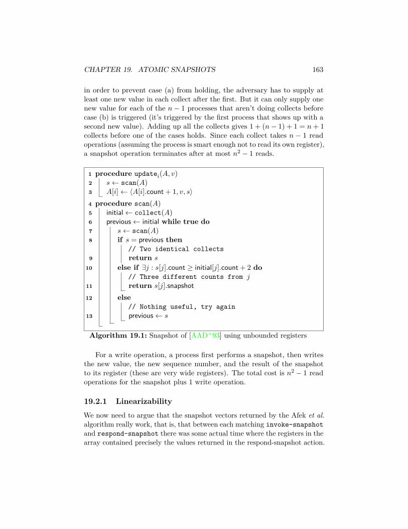
CHAPTER 19. ATOMIC SNAPSHOTS 163

in order to prevent case (a) from holding, the adversary has to supply atleast one new value in each collect after the first. But it can only supply onenew value for each of the n− 1 processes that aren’t doing collects beforecase (b) is triggered (it’s triggered by the first process that shows up with asecond new value). Adding up all the collects gives 1 + (n− 1) + 1 = n+ 1collects before one of the cases holds. Since each collect takes n − 1 readoperations (assuming the process is smart enough not to read its own register),a snapshot operation terminates after at most n2 − 1 reads.

1 procedure updatei(A, v)2 s← scan(A)3 A[i]← 〈A[i].count + 1, v, s〉4 procedure scan(A)5 initial← collect(A)6 previous← initial while true do7 s← scan(A)8 if s = previous then

// Two identical collects9 return s

10 else if ∃j : s[j].count ≥ initial[j].count + 2 do// Three different counts from j

11 return s[j].snapshot12 else

// Nothing useful, try again13 previous← s

Algorithm 19.1: Snapshot of [AAD+93] using unbounded registers

For a write operation, a process first performs a snapshot, then writesthe new value, the new sequence number, and the result of the snapshotto its register (these are very wide registers). The total cost is n2 − 1 readoperations for the snapshot plus 1 write operation.

19.2.1 Linearizability

We now need to argue that the snapshot vectors returned by the Afek et al.algorithm really work, that is, that between each matching invoke-snapshotand respond-snapshot there was some actual time where the registers in thearray contained precisely the values returned in the respond-snapshot action.

CHAPTER 19. ATOMIC SNAPSHOTS 164

We do so by assigning a linearization point to each snapshot vector, a timeat which it appears in the registers (which for correctness of the protocol hadbetter lie within the interval between the snapshot invocation and response).For snapshots obtained through case (a), take any time between the twocollects. For snapshots obtained through case (b), take the linearization pointalready assigned to the snapshot vector provided by the third write. In thelatter case we argue by induction on termination times that the linearizationpoint lies inside the snapshot’s interval.

Note that this means that all snapshots were ultimately collected by twosuccessive collects returning identical values, since any case-(b) snapshotsits on top of a finite regression of case-(b) snapshots that must end with acase-(a) snapshot. This means that any snapshot corresponds to an actualglobal state of the registers at some point in the execution, which is not trueof all snapshot algorithms. It also means that we can replace the registers inthe snapshot array with other objects that allow us to detect updates (say,counters or max registers) and still get snapshots.

In an actual execution, the fact that we are waiting for double collectswith no intervening updates means that if there are many writers, eventuallyall of them will stall waiting for a case-(a) snapshot to complete. So thatsnapshot will complete because all the writers are stuck. In a sense, requiringwriters to do snapshots first almost gives us a form of locking, but withoutthe vulnerability to failures of a real lock.

19.2.2 Using bounded registers

The simple version of the Afek et al. algorithm requires unbounded registers(since sequence numbers may grow forever). One of the reasons why thisalgorithm required so many smart people was to get rid of this assumption:the paper describes a (rather elaborate) mechanism for recycling sequencenumbers that prevents unbounded growth (see also [Lyn96, 13.3.3]). Inpractice, unbounded registers are probably not really an issue once onehas accepted very large registers, but getting rid of them is an interestingtheoretical problem.

It turns out that with a little cleverness we can drop the sequence numbersentirely. The idea is that we just need a mechanism to detect when somebodyhas done a lot of writes while a snapshot is in progress. A naive approachwould be to have sequence numbers wrap around mod m for some smallconstant modulus m; this fails because if enough snapshots happen betweentwo of my collects, I may notice none of them because all the sequencenumbers wrapped around all the way. But we can augment mod-m sequence

CHAPTER 19. ATOMIC SNAPSHOTS 165

numbers with a second handshaking mechanism that detects when a largeenough number of snapshots have occurred; this acts like the guard bit onan automobile odometer, than signals when the odometer has overflowedto prevent odometer fraud by just running the odometer forward an extramillion miles or so.

The result is the full version of Afek et al. [AAD+93]. (Our presentationhere follows [AW04, 10.3].) The key mechanism for detecting odometer fraudis a handshake, a pair of single-writer bits used by two processes to signaleach other that they have done something. Call the processes S (for same)and D (for different), and supposed we have handshake bits hS and hD. Wethen provide operations tryHandshake (signal that something is happening)and checkHandshake (check if something happened) for each process; theseoperations are asymmetric. The code is:

tryHandshake(S): hS ← hD (make the two bits the same)

tryHandshake(D): hD ← ¬hS (make the two bits different)

checkHandshake(S): return hS 6= hD (return true if D changed its bit)

checkHandshake(D): return hS = hD (return true if S changed its bit)

The intent is that checkHandshake returns true if the other processcalled tryHandshake after I did. The situation is a bit messy, however, sincetryHandshake involves two register operations (reading the other bit andthen writing my own). So in fact we have to look at the ordering of theseread and write events. Let’s assume that checkHandshake is called by S (soit returns true if and only if it sees different values). Then we have two cases:

1. checkHandshake(S) returns true. Then S reads a different value inhD from the value it read during its previous call to tryHandshake(S).It follows that D executed a write as part of a tryHandshake(D)operation in between S’s previous read and its current read.

2. checkHandshake(S) returns false. Then S reads the same value in hDas it read previously. This does not necessarily mean that D didn’twrite hD during this interval—it is possible that D is just very outof date, and did a write that didn’t change the register value—but itdoes mean that D didn’t perform both a read and a write since S’sprevious read.

How do we use this in a snapshot algorithm? The idea is that beforeperforming my two collects, I will execute tryHandshake on my end of a

CHAPTER 19. ATOMIC SNAPSHOTS 166

pair of handshake bits for every other process. After performing my twocollects, I’ll execute checkHandshake. I will also assume each update (afterperforming a snapshot) toggles a mod-2 sequence number bit on the valuestored in its segment of the snapshot array. The hope is that between thetoggle and the handshake, I detect any changes. (See [AW04, Algorithm 30]for the actual code.)

Does this work? Let’s look at cases:

1. The toggle bit for some process q is unchanged between the two snap-shots taken by p. Since the bit is toggled with each update, this meansthat an even number of updates to q′s segment occurred during theinterval between p’s writes. If this even number is 0, we are happy: noupdates means no call to tryHandshake by q, which means we don’tsee any change in q’s segment, which is good, because there wasn’t any.If this even number is 2 or more, then we observe that each of theseevents precedes the following one:

• p’s call to tryHandshake.• p’s first read.• q’s first write.• q’s call to tryHandshake at the start of its second scan.• q’s second write.• p’s second read.• p’s call to checkHandshake.

It follows that q both reads and writes the handshake bits in betweenp’s calls to tryHandshake and checkHandshake, so p correctly seesthat q has updated its segment.

2. The toggle bit for q has changed. Then q did an odd number of updates(i.e., at least one), and p correctly detects this fact.

What does p do with this information? Each time it sees that q has donea scan, it updates a count for q. If the count reaches 3, then p can determinethat q’s last scanned value is from a scan that is contained completely withinthe time interval of p’s scan. Either this is a direct scan, where q actuallyperforms two collects with no changes between them, or it’s an indirectscan, where q got its value from some other scan completely contained withinq’s scan. In the first case p is immediately happy; in the second, we observethat this other scan is also contained within the interval of p’s scan, and so

CHAPTER 19. ATOMIC SNAPSHOTS 167

(after chasing down a chain of at most n− 1 indirect scans) we eventuallyreach a direct scan contained within it that provided the actual value. Ineither case p returns the value of pair of adjacent collects with no changesbetween them that occurred during the execution of its scan operation, whichgives us linearizability.

19.3 Faster snapshots using lattice agreementThe Afek et al. algorithm and its contemporaries all require O(n2) operationsfor each snapshot. It is possible to get this bound down to O(n) using amore clever algorithm, [IMCT94] which is the best we can reasonably hopefor in the worst case given that (a) even a collect (which doesn’t guaranteeanything about linearizability) requires Θ(n) operations when implementedin the obvious way, and (b) there is a linear lower bound, due to Jayanti,Tan, and Toueg [JTT00], on a large class of wait-free objects that includessnapshot.3

The first step, due to Attiya, Herlihy, and Rachman [AHR95], is areduction to a related problem called lattice agreement.

19.3.1 Lattice agreement

A lattice is a partial order in which every pair of elements x, y has a leastupper bound x ∨ y called the join of x and y and a greatest lower boundx ∧ y called the meet of x and y. For example, we can make a lattice outof sets by letting join be union and meet be intersection; or we can make alattice out of integers by making join be max and meet be min.

In the lattice agreement problem, each process starts with an input xiand produces an output yi, where both are elements of some lattice. Therequirements of the problem are:

Comparability For all i, j, yi ≤ yj or yj ≤ yi.

Downward validity For all i, xi ≤ yi.

Upward validity For all i, yi ≤ x1 ∨ x2 ∨ x3 ∨ . . . ∨ xn.

These requirements are analogous to the requirements for consensus. Com-parability acts like agreement: the views returned by the lattice-agreementprotocol are totally ordered. Downward validity says that each process will

3But see §21.6 for a faster alternative if we allow either randomization or limits on thenumber of times the array is updated.

CHAPTER 19. ATOMIC SNAPSHOTS 168

include its own input in its output. Upward validity acts like validity: anoutput can’t include anything that didn’t show up in some input.

For the snapshot algorithm, we also demand wait-freedom: each processterminates after a bounded number of its own steps, even if other processesfail.

Note that if we are really picky, we can observe that we don’t actuallyneed meets; a semi-lattice that provides only joins is enough. In practicewe almost always end up with a full-blown lattice, because (a) we are workingwith finite sets, and (b) we generally want to include a bottom element ⊥that is less than all the other elements, to represent the “empty” state ofour data structure. But any finite join-semi-lattice with a bottom elementturns out to be a lattice, since we can define x ∧ y as the join of all elementsz such that z ≤ x and z ≤ y. We don’t use the fact that we are in a latticeanywhere, but it does save us two syllables not to have to say “semi-latticeagreement.”

19.3.2 Connection to vector clocks

The first step in reducing snapshot to lattice agreement is to have each writergenerate a sequence of increasing timestamps r1, r2, . . . , and a snapshotcorresponds to some vector of timestamps 〈t1, t2 . . . tn〉, where ti indicatesthe most recent write by pi that is included in the snapshot (in other words,we are using vector clocks again; see §6.2.3). Now define v ≤ v′ if vi ≤ v′i forall i; the resulting partial order is a lattice, and in particular we can computex ∨ y by the rule (x ∨ y)i = xi ∨ yi.

Suppose now that we have a bunch of snapshots that satisfy the com-parability requirement. This means they are totally ordered. Then we canconstruct a sequential execution by ordering the snapshots in increasing orderwith each update operation placed before the first snapshot that includesit. This sequential execution is not necessarily a linearization of the originalexecution, and a single lattice agreement object won’t support more than oneoperation for each process, but the idea is that we can nonetheless use latticeagreement objects to enforce comparability between concurrent executionsof snapshot, while doing some other tricks (exploiting, among other things,the validity properties of the lattice agreement objects) to get linearizabilityover the full execution.

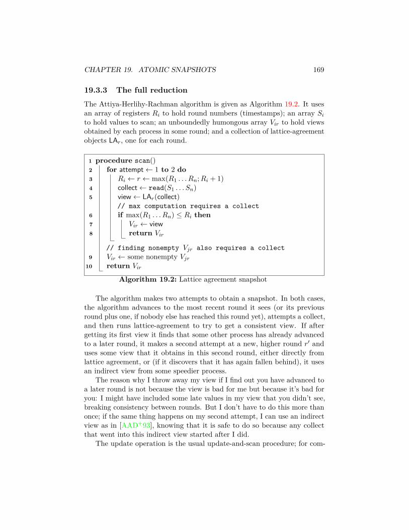
CHAPTER 19. ATOMIC SNAPSHOTS 169

19.3.3 The full reduction

The Attiya-Herlihy-Rachman algorithm is given as Algorithm 19.2. It usesan array of registers Ri to hold round numbers (timestamps); an array Sito hold values to scan; an unboundedly humongous array Vir to hold viewsobtained by each process in some round; and a collection of lattice-agreementobjects LAr, one for each round.

1 procedure scan()2 for attempt← 1 to 2 do3 Ri ← r ← max(R1 . . . Rn;Ri + 1)4 collect← read(S1 . . . Sn)5 view← LAr(collect)

// max computation requires a collect6 if max(R1 . . . Rn) ≤ Ri then7 Vir ← view8 return Vir

// finding nonempty Vjr also requires a collect9 Vir ← some nonempty Vjr

10 return Vir

Algorithm 19.2: Lattice agreement snapshot

The algorithm makes two attempts to obtain a snapshot. In both cases,the algorithm advances to the most recent round it sees (or its previousround plus one, if nobody else has reached this round yet), attempts a collect,and then runs lattice-agreement to try to get a consistent view. If aftergetting its first view it finds that some other process has already advancedto a later round, it makes a second attempt at a new, higher round r′ anduses some view that it obtains in this second round, either directly fromlattice agreement, or (if it discovers that it has again fallen behind), it usesan indirect view from some speedier process.

The reason why I throw away my view if I find out you have advanced toa later round is not because the view is bad for me but because it’s bad foryou: I might have included some late values in my view that you didn’t see,breaking consistency between rounds. But I don’t have to do this more thanonce; if the same thing happens on my second attempt, I can use an indirectview as in [AAD+93], knowing that it is safe to do so because any collectthat went into this indirect view started after I did.

The update operation is the usual update-and-scan procedure; for com-

CHAPTER 19. ATOMIC SNAPSHOTS 170

pleteness this is given as Algorithm 19.3. To make it easier to reason aboutthe algorithm, we assume that an update returns the result of the embeddedscan.

1 procedure updatei(v)2 Si ← (Si.seqno + 1, v)3 return scan()

Algorithm 19.3: Update for lattice agreement snapshot

19.3.4 Why this works

We need to show three facts:

1. All views returned by the scan operation are comparable; that is, thereexists a total order on the set of views (which can be extended to atotal order on scan operations by breaking ties using the executionorder).

2. The view returned by an update operation includes the update (thisimplies that future views will also include the update, giving the correctbehavior for snapshot).

3. The total order on views respects the execution order: if π1 and π2 arescan operations that return v1 and v2, then π1 <S π2 implies v1 ≤ v2.(This gives us linearization.)

Let’s start with comparability. First observe that any view returnedis either a direct view (obtained from LAr) or an indirect view (obtainedfrom Vjr for some other process j). In the latter case, following the chain ofindirect views eventually reaches some direct view. So all views returned fora given round are ultimately outputs of LAr and thus satisfy comparability.

But what happens with views from different rounds? The lattice-agreement objects only operate within each round, so we need to ensure thatany view returned in round r is included in any subsequent rounds. This iswhere checking round numbers after calling LAr comes in.

Suppose some process i returns a direct view; that is, it sees no higherround number in either its first attempt or its second attempt. Then atthe time it starts checking the round number in Line 6, no process has yetwritten a round number higher than the round number of i’s view (otherwise

CHAPTER 19. ATOMIC SNAPSHOTS 171

i would have seen it). So no process with a higher round number has yetexecuted the corresponding collect operation. When such a process doesso, it obtains values that are at least as large as those fed into LAr, and i’sround-r view is less than or equal to the vector of these values by upwardvalidity of LAr, and thus less than or equal to the vector of values returnedby LAr′ for r′ > r, by downward validity of LAr′ . So we have comparabilityof all direct views, which implies comparability of all indirect views as well.

To show that each view returned by a scan includes any preceding update,we observe that either a process returns its first-try scan (which includesthe update by downward validity) or it returns the results of a scan in thesecond-try round (which includes the update by downward validity in thelater round, since any collect in the second-try round starts after the updateoccurs). So no updates are missed.

Now let’s consider two scan operations π1 and π2 where π1 precedes π2in the execution. We want to show that, for the views v1 and v2 that thesescans return, v1 ≤ v2. Pick some time between when π1 finishes and π2starts, and let s be the contents of the registers at this time. Then v1 ≤ s byupward validity, since any input fed to a lattice agreement object before π1finishes was collected from a register whose value was no greater than it is ins. Similarly, s ≤ v2 by downward validity, because v2 is at least as large asthe collect value read by π2, and this is at least as large as s. So v1 ≤ s ≤ v2.

19.3.5 Implementing lattice agreement

There are several known algorithms for implementing lattice agreement,including the original algorithm of Attiya, Herlihy, and Rachman [AHR95]and an adaptive algorithm of Attiya and Fouren [AF01]. The best of them(assuming multi-writer registers) is Inoue et al.’s linear-time lattice agreementprotocol [IMCT94].

The intuition behind this protocol is to implement lattice agreementusing divide-and-conquer. The processes are organized into a tree, with eachleaf in the tree corresponding to some process’s input. Internal nodes ofthe tree hold data structures that will report increasingly large subsets ofthe inputs under them as they become available. At each internal node, adouble-collect snapshot is used to ensure that the value stored at that nodeis always the union of two values that appear in its children at the same time.This is used to guarantee that, so long as each child stores an increasingsequence of sets of inputs, the parent does so also.

Each process ascends the tree updating nodes as it goes to ensure thatits value is included in the final result. A clever data structure is used to

CHAPTER 19. ATOMIC SNAPSHOTS 172

ensure that out-of-date smaller sets don’t overwrite larger ones at any node,and the cost of using this data structure and carrying out the double-collectsnapshot at a node with m leaves below it is shown to be O(m). So the totalcost of a snapshot is O(n+ n/2 + n/4 + . . . 1) = O(n), giving the linear timebound.

Let’s now look at the details of this protocol. There are two maincomponents: the Union algorithm used to compute a new value for eachnode of the tree, and the ReadSet and WriteSet operations used to store thedata in the node. These are both rather specialized algorithms and dependon the details of the other, so it is not trivial to describe them in isolationfrom each other; but with a little effort we can describe exactly what eachcomponent demands from the other, and show that it gets it.

The Union algorithm does the usual two-collects-without change trick toget the values of the children and then stores the result. In slightly moredetail:

1. Perform ReadSet on both children. This returns a set of leaf values.

2. Perform ReadSet on both children again.

3. If the values obtained are the same in both collects, call WriteSet onthe current node to store the union of the two sets and proceed to theparent node. Otherwise repeat the preceding step.

The requirement of the Union algorithm is that calling ReadSet on agiven node returns a non-decreasing sequence of sets of values; that is, ifReadSet returns some set S at a particular time and later returns S′, thenS ⊆ S′. We also require that the set returned by ReadSet is a supersetof any set written by a WriteSet that precedes it, and that it is equal tosome such set. This last property only works if we guarantee that the valuesstored by WriteSet are all comparable (which is shown by induction on thebehavior of Union at lower levels of the tree).

Suppose that all these conditions hold; we want to show that the valueswritten by successive calls to Union are all comparable, that is, for any valuesS, S′ written by union we have S ⊆ S′ or S′ ⊆ S. Observe that S = L ∪Rand S′ = L′ ∪ R′ where L, R and L′, R′ are sets read from the children.Suppose that the Union operation producing S completes its snapshot beforethe operation producing S′. Then L ⊆ L′ (by the induction hypothesis) andR ⊆ R′, giving S ⊆ S′.

We now show how to implement the ReadSet and WriteSet operations.The main thing we want to avoid is the possibility that some large set gets

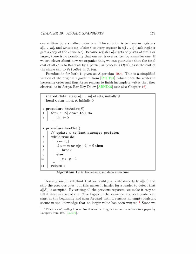
CHAPTER 19. ATOMIC SNAPSHOTS 173

overwritten by a smaller, older one. The solution is to have m registersa[1 . . .m], and write a set of size s to every register in a[1 . . . s] (each registergets a copy of the entire set). Because register a[s] gets only sets of size s orlarger, there is no possibility that our set is overwritten by a smaller one. Ifwe are clever about how we organize this, we can guarantee that the totalcost of all calls to ReadSet by a particular process is O(m), as is the cost ofthe single call to WriteSet in Union.

Pseudocode for both is given as Algorithm 19.4. This is a simplifiedversion of the original algorithm from [IMCT94], which does the writes inincreasing order and thus forces readers to finish incomplete writes that theyobserve, as in Attiya-Bar-Noy-Dolev [ABND95] (see also Chapter 16).

shared data: array a[1 . . .m] of sets, initially ∅local data: index p, initially 0

1 procedure WriteSet(S)2 for i← |S| down to 1 do3 a[i]← S

4 procedure ReadSet()// update p to last nonempty position

5 while true do6 s← a[p]7 if p = m or a[p+ 1] = ∅ then8 break9 else

10 p← p+ 1

11 return s

Algorithm 19.4: Increasing set data structure

Naively, one might think that we could just write directly to a[|S|] andskip the previous ones, but this makes it harder for a reader to detect thata[|S|] is occupied. By writing all the previous registers, we make it easy totell if there is a set of size |S| or bigger in the sequence, and so a reader canstart at the beginning and scan forward until it reaches an empty register,secure in the knowledge that no larger value has been written.4 Since we

4This trick of reading in one direction and writing in another dates back to a paper byLamport from 1977 [Lam77].

CHAPTER 19. ATOMIC SNAPSHOTS 174

want to guarantee that no reader every spends more that O(m) operationson an array of m registers (even if it does multiple calls to ReadSet), we alsohave it remember the last location read in each call to ReadSet and startthere again on its next call. For WriteSet, because we only call it once, wedon’t have to be so clever, and can just have it write all |S| ≤ m registers.

We need to show linearizability. We’ll do so by assigning a specificlinearization point to each high-level operation. Linearize each call to ReadSetat the last time that it reads a[p]. Linearize each call to WriteSet(S) at thefirst time at which a[|S|] = S and a[i] 6= ∅ for every i < |S| (in other words,at the first time that some reader might be able to find and return S); ifthere is no such time, linearize the call at the time at which it returns. Sinceevery linearization point is inside its call’s interval, this gives a linearizationthat is consistent with the actual execution. But we have to argue that itis also consistent with a sequential execution, which means that we needto show that every ReadSet operation returns the largest set among thosewhose corresponding WriteSet operations are linearized earlier.

Let R be a call to ReadSet and W a call to WriteSet(S). If R returns S,then at the time that R reads S from a[|S|], we have that (a) every registera[i] with i < |S| is non-empty (otherwise R would have stopped earlier), and(b) |S| = m or a[|S|+ 1] = ∅ (as otherwise R would have kept going afterlater reading a[|S|+ 1]. From the rule for when WriteSet calls are linearized,we see that the linearization point of W precedes this time and that thelinearization point of any call to WriteSet with a larger set follows it. Sothe return value of R is consistent.

The payoff: unless we do more updates than snapshots, don’t want toassume multi-writer registers, are worried about unbounded space, have abeef with huge registers, or care about constant factors, it costs no moretime to do a snapshot than a collect. So in theory we can get away withassuming snapshots pretty much wherever we need them.

19.4 Practical snapshots using LL/SCThough atomic registers are enough for snapshots, it is possible to geta much more efficient snapshot algorithm using stronger synchronizationprimitives. An algorithm of Riany, Shavit, and Touitou [RST01] uses load-linked/store-conditional objects to build an atomic snapshot protocolwith linear-time snapshots and constant-time updates using small registers.We’ll give a sketch of this algorithm here.

The RST algorithm involves two basic ideas: the first is a snapshot

CHAPTER 19. ATOMIC SNAPSHOTS 175

algorithm for a single scanner (i.e., only one process can do snapshots) inwhich each updater maintains two copies of its segment, a high copy (thatmay be more recent than the current scan) and a low copy (that is guaranteedto be no more recent than the current scan). The idea is that when a scan isin progress, updaters ensure that the values in memory at the start of thescan are not overwritten before the scan is completed, by copying them tothe low registers, while the high registers allow new values to be writtenwithout waiting for the scan to complete. Unbounded sequence numbers,generated by the scanner, are used to tell which values are recent or not.

As long as there is only one scanner, nothing needs to be done to ensurethat all scans are consistent, and indeed the single-scanner algorithm can beimplemented using only atomic registers. But extending the algorithm tomultiple scanners is tricky. A simple approach would be to keep a separatelow register for each concurrent scan—however, this would require up to nlow registers and greatly increase the cost of an update. Instead, the authorsdevise a mechanism, called a coordinated collect, that allows the scannerscollectively to implement a sequence of virtual scans that do not overlap.Each virtual scan is implemented using the single-scanner algorithm, with itsoutput written to a common view array that is protected from inconsistentupdates using LL/SC operations (CAS also works). A scanner participatesin virtual scans until it obtains a virtual scan that is useful to it (this meansthat the virtual scan has to take place entirely within the interval of theprocess’s actual scan operation); the simplest way to arrange this is to haveeach scanner perform two virtual scans and return the value obtained by thesecond one.

The paper puts a fair bit of work into ensuring that only O(n) viewarrays are needed, which requires handling some extra special cases whereparticularly slow processes don’t manage to grab a view before it is reallocatedfor a later virtual scan. We avoid this complication by simply assuming anunbounded collection of view arrays; see the paper for how to do this right.

A more recent paper by Fatourou and Kallimanis [FK07] gives improvedtime and space complexity using the same basic technique.

19.4.1 Details of the single-scanner snapshot

The single-scanner snapshot is implemented using a shared currSeq variable(incremented by the scanner but used by all processes) and an array memory ofn snapshot segments, each of which is divided into a high and low componentconsisting of a value and a timestamp. Initially, currSeq is 0, and all memorylocations are initialized to (⊥, 0). This part of the algorithm does not require

CHAPTER 19. ATOMIC SNAPSHOTS 176

LL/SC.A call to scan copies the first of memory[j].high or memory[j].low that

has a sequence number less than the current sequence number. Pseudocodeis given as Algorithm 19.5.

1 procedure scan()2 currSeq← currSeq + 13 for j ← 0 to n− 1 do4 h← memory[j].high5 if h.seq < currSeq then6 view[j]← h.value7 else8 view[j]← memory[j].low.value

Algorithm 19.5: Single-scanner snapshot: scan

The update operation for process i cooperates by copying memory[i].highto memory[i].low if it’s old.

The update operation always writes its value to memory[i].high, butpreserves the previous value in memory[i].low if its sequence number indicatesthat it may have been present at the start of the most recent call to scan.This means that scan can get the old value if the new value is too recent.Pseudocode is given in Algorithm 19.6.

1 procedure update()2 seq← currSeq3 h← memory[i].high4 if h.seq 6= seq then5 memory[i].low← h

6 memory[i].high← (value, seq)

Algorithm 19.6: Single-scanner snapshot: update

To show this actually works, we need to show that there is a linearizationof the scans and updates that has each scan return precisely those valueswhose corresponding updates are linearized before it. The ordering is basedon when each scan operation S increments currSeq and when each updateoperation U reads it; specifically:

• If U reads currSeq after S increments it, then S < U .

CHAPTER 19. ATOMIC SNAPSHOTS 177

• If U reads currSeq before S increments it and S reads memory[i].high(where i is the process carrying out U) before U writes it, then S < U .

• If U reads currSeq before S increments it, but S reads memory[i].highafter U writes it, then U < S.

Updates are ordered based on intervening scans (i.e., U1 < U2 if U1 < Sand S < U2 by the above rules), or by the order in which they read currSeqif there is no intervening scan.

To show this is a linearization, we need first to show that it extends theordering between operations in the original schedule. Each of the above ruleshas π1 < π2 only if some low-level operation of π1 precedes some low-leveloperation of π2, with the exception of the transitive ordering of two updateevents with an intervening scan. But in this last case we observe that ifU1 < S, then U1 writes memory[i].high before S reads it, so if U1 precedesU2 in the actual execution, U2 must write memory[i].high after S reads it,implying S < U2.

Now we show that the values returned by scan are consistent with thelinearization ordering; that, is, for each i, scan copies to view[i] the value inthe last update by process i in the linearization. Examining the code for scan,we see that a scan operation S takes memory[i].high if its sequence numberis less than currSeq, i.e., if the update operation U that wrote it read currSeqbefore S incremented it and wrote memory[i].high before S read it; this givesU < S. Alternatively, if scan takes memory[i].low, then memory[i].low wascopied by some update operation U ′ from the value written to memory[i].highby some update U that read currSeq before S incremented it. Here U ′ musthave written memory[i].high before S read it (otherwise S would have takenthe old value left by U) and since U precedes U ′ (being an operation of thesame process) it must therefor also have written memory[i].high before S readit. So again we get the first case of the linearization ordering and U < S.

So far we have shown only that S obtains values that were linearizedbefore it, but not that it ignores values that were linearized after it. So nowlet’s consider some U with S < U . Then one of two cases holds:

• U reads currSeq after S increments it. Then U writes a sequencenumber in memory[i].high that is greater than or equal to the currSeqvalue used by S; so S returns memory[i].low instead, which can’t havea sequence number equal to currSeq and thus can’t be U ’s value either.

• U reads currSeq before S increments it but writes memory[i].high afterS reads it. Now S won’t return U ’s value from memory[i].high (it didn’t

CHAPTER 19. ATOMIC SNAPSHOTS 178

read it), and won’t get it from memory[i].low either (because the valuethat is in memory[i].high will have seq < currSeq, and so S will takethat instead).

So in either case, if S < U , then S doesn’t return U ’s value. Thisconcludes the proof of correctness.

19.4.2 Extension to multiple scanners

See the paper for details.The essential idea: view now represents a virtual scan viewr generated

cooperatively by all the scanners working together in some asynchronousround r. To avoid conflicts, we update viewr using LL/SC or compare-and-swap (so that only the first scanner to write wins), and pretend that readsof memory[i] by losers didn’t happen. When viewr is full, start a new virtualscan and advance to the next round (and thus the next viewr+1).

19.5 ApplicationsHere we describe a few things we can do with snapshots.

19.5.1 Multi-writer registers from single-writer registers

One application of atomic snapshot is building multi-writer registers fromsingle-writer registers. The idea is straightforward: to perform a write, aprocess does a snapshot to obtain the maximum sequence number, tags itsown value with this sequence number plus one, and then writes it. A readconsists of a snapshot followed by returning the value associated with thelargest sequence number (breaking ties by process id). (See [Lyn96, §13.5]for a proof that this actually works.) This requires using a snapshot thatdoesn’t use multi-writer registers, and turns out to be overkill in practice;there are simpler algorithms that give O(n) cost for reads and writes basedon timestamps (see [AW04, 10.2.3]).

With additional work, it is even possible to eliminate the requirementof multi-reader registers, and get a simulation of multi-writer multi-readerregisters that goes all the way down to single-writer single-read registers, oreven single-writer single-reader bits. See [AW04, §§10.2.1–10.2.2] or [Lyn96,§13.4] for details.

CHAPTER 19. ATOMIC SNAPSHOTS 179

19.5.2 Counters

Given atomic snapshots, it’s easy to build a counter (supporting increment,decrement, and read operations); or, in more generality, a generalized counter(supporting increments by arbitrary amounts); or, in even more generality,an object supporting any collection of commutative and associative updateoperations (as long as these operations don’t return anything). The ideais that each process stores in its segment the total of all operations it hasperformed so far, and a read operation is implemented using a snapshotfollowed by summing the results. This is a case where it is reasonableto consider multi-writer registers in building the snapshot implementation,because there is not necessarily any circularity in doing so.

19.5.3 Resilient snapshot objects

The previous examples can be generalized to objects with operations thateither read the current state of the object but don’t update it or update thestate but return nothing, provided the update operations either overwrite eachother (so that Cxy = Cy or Cyx = Cx) or commute (so that Cxy = Cyx).

This was shown by Aspnes and Herlihy [AH90b] and improved on byAnderson and Moir [AM93] by eliminating unbounded space usage. An-derson and Moir also defined the terms snapshot objects for those withseparate read and update operations and resilience for the property thatall operations commute or overwrite. The basic idea underneath both ofthese papers is to use the multi-writer register construction given above, butbreak ties among operations with the same sequence numbers by first placingoverwritten operations before overwriting operations and only then usingprocess ids.

This almost shows that snapshots can implement any object with con-sensus number 1 where update operations return nothing, because an objectthat is not resilient violates the commute-or-overwrite condition in someconfiguration has consensus number at least 2 (see §18.1.2)—in Herlihy’sterminology, non-resilient objects have interfering operations. It doesn’t quitework (as observed in the Anderson-Moir paper), because the tie-breakingprocedure assumes a static ordering on which operations overwrite eachother, so that given operations x and y where y overwrites x, y overwritesx in any configuration. But there may be objects with a dynamic orderingto how operations interfere, where y overwrites x in some configuration, xoverwrites y in another, and perhaps even the two operations commute inyet another. This prevents us from achieving consensus, but also breaks the

CHAPTER 19. ATOMIC SNAPSHOTS 180

tie-breaking technique. So it may be possible that there are objects withconsensus number 1 and no-return updates that we still can’t implementusing only registers.

Chapter 20

Lower bounds onperturbable objects

Being able to do snapshots in linear time means that we can build linearizablecounters, generalized counters, max registers, and so on, in linear time, byhaving each reader take a snapshot and combine the contributions of eachupdater using the appropriate commutative and associative operation. Anatural question is whether we can do better by exploiting the particularfeatures of these objects.

Unfortunately, the Jayanti-Tan-Toueg [JTT00] lower bound for per-turbable objects says each of these objects requires n− 1 space and n− 1steps for a read operation in the worst case, for any solo-terminating deter-ministic implementation from historyless objects. Like Burns-Lynch, thisis a worst-case bound based on a covering argument, so it may be possibleto evade it in some cases using either randomization or a restriction on thelength of an execution (see Chapter 21).

Perturbable means that the object has a particular property that makesthe proof work, essentially that the outcome of certain special executionscan be changed by stuffing lots of extra update operations in the middle (seebelow for details).

Solo-terminating means that a process finishes its current operationin a finite number of steps if no other process takes steps in between; it is amuch weaker condition, for example, than wait-freedom.

Historyless objects are those for which any operation either neverchanges the state (like a read, but it could be weaker) or always sets thestate to a value that depends only on the operation and not the previousvalue (like a write, but it may also return some information about the old

181

CHAPTER 20. LOWER BOUNDS ON PERTURBABLE OBJECTS 182

state). The point of historyless objects is that covering arguments work forthem: if there is a process with a pending update operations on some object,the adversary can use it at any time to wipe out the state of the object andhide any previous operations from any process except the updater (who, ina typical covering argument, is quietly killed to keep it from telling anybodywhat it saw).

Atomic registers are a common example of a historyless object: the readnever changes the state, and the write always replaces it. Swap objects(with a swap operation that writes a new state while returning the old state)are the canonical example, since they can implement any other historylessobject (and even have consensus number 2, showing that even extra consensuspower doesn’t necessarily help here). Test-and-sets (which are basically one-bit swap objects where you can only swap in 1) are also historyless. Incontrast, anything that looks like a counter or similar object where the newstate is a combination of the old state and the operation is not historyless.This is important because many of these objects turn out to be perturbable,and if they were also historyless, we’d get a contradiction.

Below is a sketch of the proof. See the original paper [JTT00] for moredetails.

The basic idea is to build a sequence of executions of the form ΛkΣkπ,where Λk is a preamble consisting of various complete update operations andk incomplete update operations by processes p1 through pn−1, Σk deliversk delayed writes from the incomplete operations in Λk, and π is a readoperation by pn. To make our life easier, we’ll assume that π performs onlyread steps.1

We’ll expand ΛkΣk to Λk+1Σk+1 by inserting new operations in betweenΛk and Σk, and argue that because those operations can change the valuereturned by π, one of them must write an object not covered in Σk, whichwill (after some more work) allow us to cover yet another object.

In order for these covered objects to keep accumulating, the reader hasto keep looking at them. To a first approximation, this means that we wantthe first k reads done by π to be from objects written in Σk: since thevalues seen by the reader for these objects never change, the (deterministic)

1The idea is that if π does anything else, then the return values of other steps canbe simulated by doing a read in place of the first step and using the property of beinghistoryless to compute the return values of subsequent steps. There is still a possibleobjection that we might have some historyless objects that don’t even provide read steps.The easiest way to work around this is to assume that our objects do in fact provide a readstep, because taking the read step away isn’t going to make implementing the candidateperturbable object any easier.

CHAPTER 20. LOWER BOUNDS ON PERTURBABLE OBJECTS 183

reader will continue to read them even as we add more operations before Σk.Unfortunately, this does not quite match all possible cases, because it maybe that π performs useless reads of objects that aren’t covered in Σk butthat aren’t written to by anybody anyway. So we have the more technicalcondition that π has an initial prefix that only includes covered reads anduseless reads: formally, there is a prefix π′ of π that includes at least one readoperation of every object covered by Σk, such that any other read operationin π′ reads an object whose state cannot be changed by any step that can beperformed by any sequence of operations by processes p1 through pn−1 thatcan be inserted between Λk and Σkπ.

The induction hypothesis is that an execution ΛkΣk with these propertiesexists for each k ≤ n− 1.

For the base case, Λ0Σ0 = 〈〉. This covers 0 reads by π.For the induction step, we start with ΛkΣk, and look for a sequence

of operations γ that we can insert in between Λk and Σk that changeswhat π returns in ΛkγΣkπ from what it returned in ΛkγΣk. This is whereperturbability comes in: an object is defined to be perturbable if such asequence γ always exists.

Some examples of γ:

• For a snapshot object, let γ write to a component that is not writtento by any of the operations in Σk.

• For a max register, let γ include a bigger write than all the others.

• For a counter, let γ include at least n increments. The same works fora mod-m counter if m is at least 2n. (Why n increments? With fewerincrements, we can make π return the same value by being sneakyabout when the partial increments represented in Σk are linearized.)

In contrast, historyless objects (including atomic registers) are not per-turbable: if Σk includes a write that sets the value of the object, no set ofoperations inserted before it will change this value. This is good, because weknow that it only takes one atomic register to implement an atomic register.

Assuming that our object is perturbable, now we want to use the existenceof γ to generate our bigger execution Λk+1Σk+1. As in the Burns-Lynchmutex bound [BL93], we will be arguing that γ must include a write to anobject that is not covered by the k delayed writes. Also as in Burns-Lynch,it turns out that it is not enough just to delay this particular write, becauseit might not cover the specific object we want.

Instead, we look for an alternative γ′ that changes the value of the earliestobject read by π that can be changed. We know that some such γ′ exists,

CHAPTER 20. LOWER BOUNDS ON PERTURBABLE OBJECTS 184

because γ writes to some such object, so there must be a first place in theexecution of π where the output of an object can change, and there must besome γ′ that makes that change. Note however that γ′ that hits that earliestobject need not be the same as the γ used to demonstrate perturbability,and indeed it may be that γ′ is very different from γ—in particular, it maybe much longer.

So now we expand γ′ = αβδ, where β is the magic write to the uncoveredobject, and let Λk+1 = Λkαδ′ and Σk+1 = βΣk, where δ′ consists of runningall incomplete operations in α except the one that include β to completion.We’ve now covered k+ 1 distinct objects in Σk. It remains only to show thatthe technical condition that any uncovered object that π reads before readingall the covered objects can’t have its value changed by inserting additionaloperations.

Suppose that there is a sequence of operations κ such that Λk+1κ changesone of these forbidden uncovered objects. But Λk+1κ = Λkακ, and soγ′′ = ακ changes an object that either (a) can’t be changed because of thetechnical condition in the induction hypothesis for k, or (b) changes an objectthat π reads before the object covered by β. In the second case, this γ′′changes an earlier object that γ′, contradicting the choice of γ′.

It follows that we do in fact manage to cover k+1 objects while satisfyingthe technical condition, and the induction hypothesis holds for k + 1.

We can repeat this step until we’ve covered n− 1 objects. This impliesthat there are at least n − 1 objects (the space lower bound), and in theworst case some reader reads all of them (the step complexity lower bound).

Chapter 21

Restricted-use objects

The Jayanti-Tan-Toueg bound puts a hard floor under the worst-case com-plexity of almost anything interesting we’d like to do wait-free in a systemthat provides only historyless objects as primitives. As with the consensus hi-erarchy lower bounds, we could interpret this as a reason to demand strongerprimivitives. Or we could look for ways to bypass the JTT bound.

One approach is to modify our target objects so that they are no longerperturbable. This can be done by limiting their use: a counter or max registerthat can only change its value a limited number of times is not perturbable,because once we hit the limit, there is no perturbing sequence of operationsthat we can insert between Λk and Σk in the JTT execution that changesthe value returned by the eventual reader. This observation motivated aline of work on restricted-use max registers [AACH12] and restricted-usesnapshots [AACHE15] that have polylogarithmic worst-case individual stepcomplexity assuming a polynomial limit on updates. While restricted-useobjects might not be all that exciting on their own, they in turn have servedas building blocks for implementations of snapshots with polylogarithmicexpected individual step complexity [ACH13] or polylogarithmic amortizedindividual step complexity [BHMT20].

In this chapter, we will concentrate on the original restricted-use maxregister construction of Aspnes, Attiya, and Censor-Hillel [AACH12], andits extension to give restricted-use snapshots by Aspnes et al. [AACHE15].

21.1 Max registersWe will start by implementing a restricted-use max register [AACH12], forwhich read operation returns the largest value previously written, as opposed

185

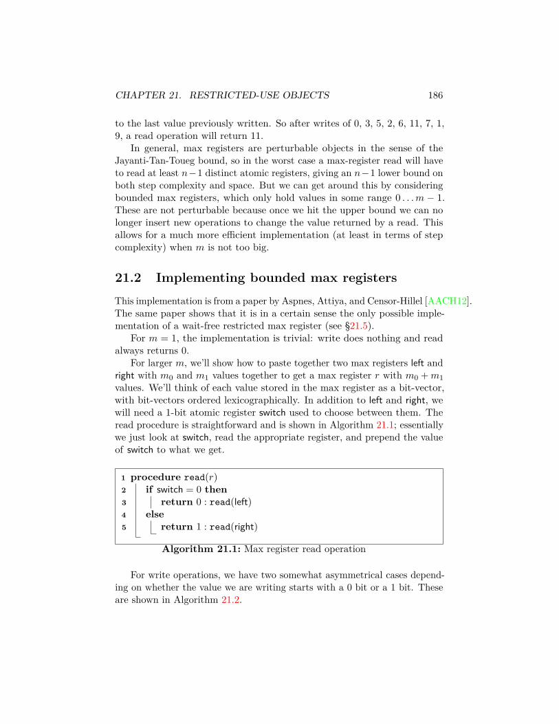
CHAPTER 21. RESTRICTED-USE OBJECTS 186

to the last value previously written. So after writes of 0, 3, 5, 2, 6, 11, 7, 1,9, a read operation will return 11.

In general, max registers are perturbable objects in the sense of theJayanti-Tan-Toueg bound, so in the worst case a max-register read will haveto read at least n−1 distinct atomic registers, giving an n−1 lower bound onboth step complexity and space. But we can get around this by consideringbounded max registers, which only hold values in some range 0 . . .m − 1.These are not perturbable because once we hit the upper bound we can nolonger insert new operations to change the value returned by a read. Thisallows for a much more efficient implementation (at least in terms of stepcomplexity) when m is not too big.

21.2 Implementing bounded max registersThis implementation is from a paper by Aspnes, Attiya, and Censor-Hillel [AACH12].The same paper shows that it is in a certain sense the only possible imple-mentation of a wait-free restricted max register (see §21.5).

For m = 1, the implementation is trivial: write does nothing and readalways returns 0.

For larger m, we’ll show how to paste together two max registers left andright with m0 and m1 values together to get a max register r with m0 +m1values. We’ll think of each value stored in the max register as a bit-vector,with bit-vectors ordered lexicographically. In addition to left and right, wewill need a 1-bit atomic register switch used to choose between them. Theread procedure is straightforward and is shown in Algorithm 21.1; essentiallywe just look at switch, read the appropriate register, and prepend the valueof switch to what we get.

1 procedure read(r)2 if switch = 0 then3 return 0 : read(left)4 else5 return 1 : read(right)

Algorithm 21.1: Max register read operation

For write operations, we have two somewhat asymmetrical cases depend-ing on whether the value we are writing starts with a 0 bit or a 1 bit. Theseare shown in Algorithm 21.2.

CHAPTER 21. RESTRICTED-USE OBJECTS 187

1 procedure write(r, 0x)2 if switch = 0 then3 write(left, x)

4 procedure write(r, 1x)5 write(right, x)6 switch← 1

Algorithm 21.2: Max register write operations

The intuition is that the max register is really a big tree of switchvariables, and we store a particular bit-vector in the max register by settingto 1 the switches needed to make read follow the path corresponding tothat bit-vector. The procedure for writing 0x tests switch first, because onceswitch gets set to 1, any 0x values are smaller than the largest value, and wedon’t want them getting written to left where they might confuse particularlyslow readers into returning a value we can’t linearize. The procedure forwriting 1x sets switch second, because (a) it doesn’t need to test switch, since1x always beats 0x, and (b) it’s not safe to send a reader down into rightuntil some value has actually been written there.

It’s easy to see that read and write operations both require exactlyone operation per bit of the value read or written. To show that we getlinearizability, we give an explicit linearization ordering (see the paper for afull proof that this works):

1. All operations that read 0 from switch go in the first pile.

(a) Within this pile, we sort operations using the linearization orderingfor left.

2. All operations that read 1 from switch or write 1 to switch go in thesecond pile, which is ordered after the first pile.

(a) Within this pile, operations that touch right are ordered usingthe linearization ordering for right. Operations that don’t (whichare the “do nothing” writes for 0x values) are placed consistentlywith the actual execution order.

To show that this gives a valid linearization, we have to argue first thatany read operation returns the largest earlier write argument and that wedon’t put any non-concurrent operations out of order.

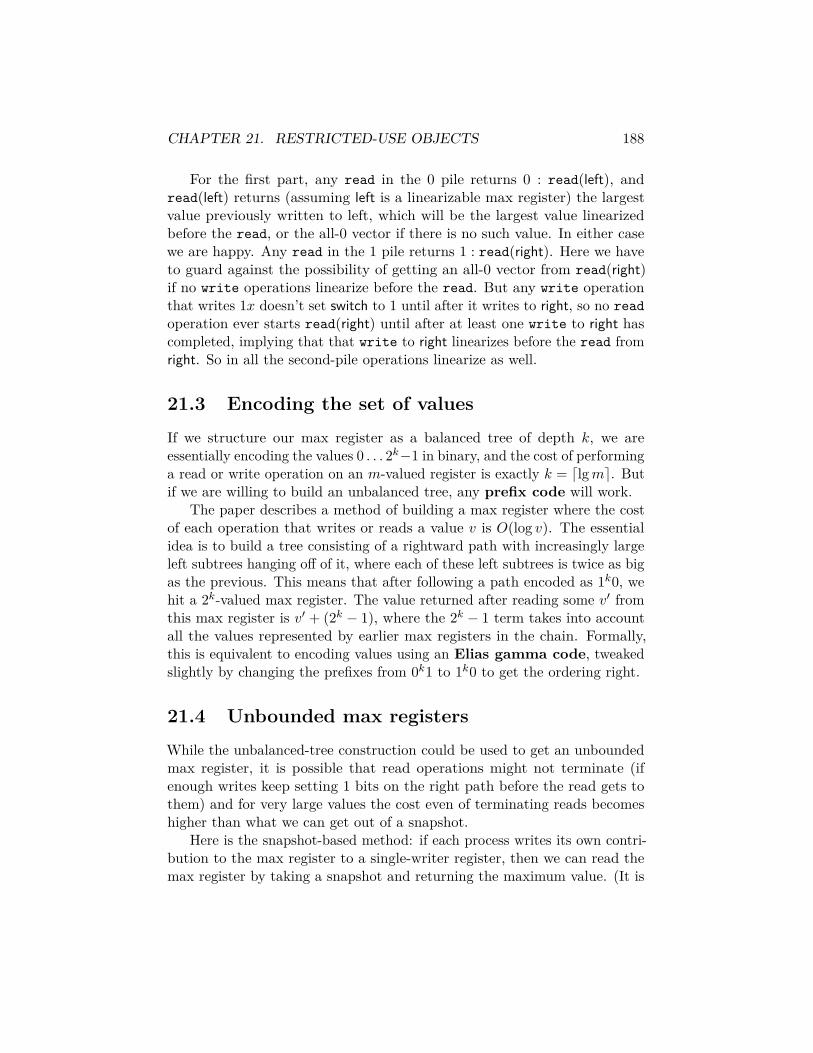
CHAPTER 21. RESTRICTED-USE OBJECTS 188

For the first part, any read in the 0 pile returns 0 : read(left), andread(left) returns (assuming left is a linearizable max register) the largestvalue previously written to left, which will be the largest value linearizedbefore the read, or the all-0 vector if there is no such value. In either casewe are happy. Any read in the 1 pile returns 1 : read(right). Here we haveto guard against the possibility of getting an all-0 vector from read(right)if no write operations linearize before the read. But any write operationthat writes 1x doesn’t set switch to 1 until after it writes to right, so no readoperation ever starts read(right) until after at least one write to right hascompleted, implying that that write to right linearizes before the read fromright. So in all the second-pile operations linearize as well.

21.3 Encoding the set of valuesIf we structure our max register as a balanced tree of depth k, we areessentially encoding the values 0 . . . 2k−1 in binary, and the cost of performinga read or write operation on an m-valued register is exactly k = dlgme. Butif we are willing to build an unbalanced tree, any prefix code will work.

The paper describes a method of building a max register where the costof each operation that writes or reads a value v is O(log v). The essentialidea is to build a tree consisting of a rightward path with increasingly largeleft subtrees hanging off of it, where each of these left subtrees is twice as bigas the previous. This means that after following a path encoded as 1k0, wehit a 2k-valued max register. The value returned after reading some v′ fromthis max register is v′ + (2k − 1), where the 2k − 1 term takes into accountall the values represented by earlier max registers in the chain. Formally,this is equivalent to encoding values using an Elias gamma code, tweakedslightly by changing the prefixes from 0k1 to 1k0 to get the ordering right.

21.4 Unbounded max registersWhile the unbalanced-tree construction could be used to get an unboundedmax register, it is possible that read operations might not terminate (ifenough writes keep setting 1 bits on the right path before the read gets tothem) and for very large values the cost even of terminating reads becomeshigher than what we can get out of a snapshot.

Here is the snapshot-based method: if each process writes its own contri-bution to the max register to a single-writer register, then we can read themax register by taking a snapshot and returning the maximum value. (It is

CHAPTER 21. RESTRICTED-USE OBJECTS 189

not hard to show that this is linearizable.) This gives an unbounded maxregister with read and write cost O(n). So by choosing this in preferenceto the balanced tree when m is large, the cost of either operation on a maxregister is min (dlgme , O(n)).

We can combine this with the unbalanced tree by terminating the rightpath with a snapshot-based max register. This gives a cost for reads andwrites of values v of O(min(log v, n)).

21.5 Lower boundThe min(dlgme , n− 1) cost of a max register read turns out to be exactlyoptimal. Intuitively, we can show by a covering argument that once someprocess attempts to write to a particular atomic register, then any subsequentwrites convey no additional information (because they can be overwritten bythe first delayed write)—so in effect, no algorithm can use get more thanone bit of information out of each atomic register. But as always, turningthis intuition into an actual proof requires a bit more work.

We will consider solo-terminating executions in which n− 1 writers doany number of max-register writes in some initial prefix Λ, followed by asingle max-register read π by process pn. Let T (m,n) be the optimal readercost for executions with this structure with m values, and let r be the firstregister read by process pn, assuming it is running an algorithm optimizedfor this class of executions (we do not even require it to be correct for otherexecutions).

We are now going split up our set of values based on which will cause awrite operation to write to r. Let Sk be the set of all sequences of writes thatonly write values ≤ k. Let t be the smallest value such that some executionin St writes to r (there must be some such t, or our reader can omit readingr, which contradicts the assumption that it is optimal).

Case 1 Since t is smallest, no execution in St−1 writes to r. If we restrictwrites to values ≤ t − 1, we can omit reading r, giving T (t, n) ≤T (m,n)− 1 or T (m,n) ≥ T (t, n) + 1.

Case 2 Let α be some execution in St that writes to r.

• Split α as α′δβ where δ is the first write to r by some process pi.• Construct a new execution α′η by letting all the max-register

writes except the one performing δ finish.

CHAPTER 21. RESTRICTED-USE OBJECTS 190

• Now consider any execution α′ηγδ, where γ is any sequence ofmax-register writes with values ≥ t that excludes pi and pn. Thenpn always sees the same value in r following these executions,but otherwise (starting after α′η) we have an (n − 1)-processmax-register with values t through m− 1.

• Omit the read of r again to get T (m,n) ≥ T (m− t, n− 1) + 1.

We’ve shown the recurrence T (m,n) ≥ mint(max(T (t, n), T (m−t, n)))+1,with base cases T (1, n) = 0 and T (m, 1) = 0. The solution to this recurrenceis exactly min(dlgme , n− 1), which is the same, except for a constant factoron n, as the upper bound we got by choosing between a balanced tree forsmall m and a snapshot for m ≥ 2n−1. For small m, the recursive split weget is also the same as in the tree-based algorithm: call the r register switchand you can extract a tree from whatever algorithm somebody gives you. Sothis says that the tree-based algorithm is (up to choice of the tree) essentiallythe unique optimal bounded max register implementation for m ≤ 2n−1.

It is also possible to show lower bounds on randomized implementationsof max registers and other restricted-use objects. See [AACH12, ACAH16,HK14] for examples.

21.6 Max-register snapshotsWith some tinkering, it’s possible to extend the max-register constructionto get an array of max registers that supports snapshots. The descriptionin this section follows [AACHE15], with some updates to fix a bug noted inthe original paper in an erratum published by the authors [AACHE18].

Formally, a max array is an object a that supports an operationwrite(a, i, v) that sets a[i] ← max(v, a[i]), and an operation read(a) thatreturns a snapshot of all components of the array. The first step in buildingthis beast is to do it for two components. The resulting 2-component maxarray can then be used as a building block for larger max arrays and forfast restricted-used snapshots in general.

A k × ` max array a is one that permits values in the range 0 . . . k − 1in a[0] and 0 . . . `− 1 in a[1]. We think of a[0] as the head of the max arrayand a[1] as the tail. We’ll show how to construct such an object recursivelyfrom smaller objects of the same type, analogous to the construction of anm-valued max register (which we can think of as a m× 1 max array). Theidea is to split head into two pieces left and right as before, while representingtail as a master copy stored in a max register at the top of the tree plus

CHAPTER 21. RESTRICTED-USE OBJECTS 191

cached copies at every internal node. These cached copies are updated byreaders at times carefully chosen to ensure linearizability.

The base of the construction is an `-valued max register r, used directlyas a 1× ` max array; this is the case where the head component is trivial andwe only need to store a.tail = r. Here calling write(a, 0, v) does nothing,while write(a, 1, v) maps to write(r, v), and read(a) returns 〈0, read(r)〉.

For larger values of k, paste a kleft× ` max array left and a kright× ` maxarray right together to get a (kleft + kright)× ` max array. This constructionuses a switch variable as in the basic construction, along with an `-valuedmax register tail that is used to store the value of a[1].

Calls to write(a, 0, v) and read(a) follow the structure of the correspond-ing operations for a simple max register, with some extra work in read tomake sure that the value in tail propagates into left and right as needed toensure the correct value is returned.

A call to write(a, 1, v) operation writes tail directly, and then callsread(a) to propagate the new value as well.1

Pseudocode is given in Algorithm 21.3.The individual step complexity of each operation is easily computed.

Assuming a balanced tree, write(a, 0, v) takes exactly dlg ke steps, whilewrite(a, 1, v) costs exactly dlg `e steps plus the cost of read(a). Readoperations are more complicated. In the worst case, we have two reads ofa.tail and a write to a.right[1] at each level, plus up to two operations ona.switch, for a total cost of at most (3dlg ke − 1)(dlg `e+ 2) = O(log k log `)steps. This dominates other costs in write(a, 1, v), so the asymptotic costof both write and read operations is O(log k log `).

In the special case where k = `, both writes and reads have their stepcomplexities squared compared to a single-component k-valued max register.

21.6.1 Linearizability

In broad outline, the proof of linearizability follows the proof for a simplemax register. But as with snapshots, we have to show that the ordering ofthe head and tail components are consistent.

The key observation is the following lemma.

Lemma 21.6.1. Fix some execution of a max array a implemented as inAlgorithm 21.3. Suppose this execution contains a read(a) operation πleft

1This call to read(a) was omitted in the original published version of the algo-rithm [AACHE15], but was added in an erratum by the authors [AACHE18]. Without it,the implementation can violate linearizability in some executions.

CHAPTER 21. RESTRICTED-USE OBJECTS 192

1 procedure write(a, i, v)2 if i = 0 then3 if v < kleft then4 if a.switch = 0 then5 write(a.left, 0, v)6 else7 write(a.right, 0, v − kleft)8 a.switch← 19 else

10 write(a.tail, v)11 read(a)

12 procedure read(a)13 x← read(a.tail)14 if a.switch = 0 then15 write(a.left, 1, x)16 return read(a.left)17 else18 x← read(a.tail)19 write(a.right, 1, x)20 return 〈kleft, 0〉+ read(a.right)

Algorithm 21.3: Recursive construction of a 2-component max array

CHAPTER 21. RESTRICTED-USE OBJECTS 193

that returns vleft from a.left and a read(a) operation πright that returns vrightfrom a.right. Then vleft[1] ≤ vright[1].

Proof. Both vleft[1] and vright[1] are values that were previously written totheir respective max arrays by read(a) operations (such writes necessarilyexist because any process that reads a.left or a.right writes a.left[1] or a.right[1]first). From examining the code, we have that any value written to a.left[1]was read from a.tail before a.switch was set to 1, while any value written toa.right[1] was read from a.tail after a.switch was set to 1. Since max-registerreads are non-decreasing, we have than any value written to a.left[1] is lessthan or equal to any value written to a.right[1], proving the claim.

The rest of the proof is tedious but straightforward: we linearize theread(a) and write(a[0]) operations as in the max-register proof, then fitthe write(a[1]) operations in based on the tail values of the reads. The fullresult is:

Theorem 21.6.2. If a.left and a.right are linearizable max arrays, and a.tailis a linearizable max register, then Algorithm 21.3 implements a linearizablemax array.

It’s worth noting that the same unbalanced-tree construction used in§§21.3 and 21.4 can be used here as well. This makes the step complexity forread(a) scale as O(log v[0] log v[1]), where v is the value returned. For writesthe step complexity may depend in a complicated way on what values arebeing written and to which side, but in the worst case, it is O(log v[0] log v[1]),where v is the value in the register when the write finishes. (This is aconsequence of the embedded read(a) in write(a, 1, v).)

21.7 Restricted-use snapshotsTo build an ordinary snapshot object from 2-component max arrays, weconstruct a balanced binary tree in which each leaves holds a pointer toan individual snapshot element and each internal node holds a pointer to apartial snapshot containing all of the elements in the subtree of which it isthe root. The pointers themselves are non-decreasing indices into arrays ofvalues that consist of ordinary (although possibly very wide) atomic registers.

When a process writes a new value to its component of the snapshotobject, it increases the pointer value in its leaf and then propagates the newvalue up the tree by combining together partial snapshots at each step, using2-component max arrays to ensure linearizability. The resulting algorithm

CHAPTER 21. RESTRICTED-USE OBJECTS 194

is similar in many ways to the lattice agreement procedure of Inoue etal. [IMCT94] (see §19.3.5), except that it uses a more contention-tolerantsnapshot algorithm than double collects and we allow processes to updatetheir values more than once. It is also similar to the f-array constructionof Jayanti [Jay02] for efficient computation of array aggregates (sum, min,max, etc.) using LL/SC, the main difference being that because the indexvalues are non-decreasing, max arrays can substitute for LL/SC.

Each node in the tree except the root is represented by one componentof a 2-component max array that we can think of as being owned by itsparent, with the other component being the node’s sibling in the tree. Topropagate a value up the tree, at each level the process takes a snapshotof the two children of the node and writes the sum of the indices to thenode’s component in its parent’s max array (or to an ordinary max registerif we are at the root). Before doing this last write, a process will combinethe partial snapshots from the two child nodes and write the result intoa separate array indexed by the sum. In this way any process that readsthe node’s component can obtain the corresponding partial snapshot in asingle register operation. At the root this means that the cost of obtaininga complete snapshot is dominated by the cost of the max-register read, atO(log v), where v is the number of updates ever performed.

A picture of this structure, adapted from the proceedings version of [AACHE15],appears in Figure 21.1. The figure depicts an update in progress, with redvalues being the new values written as part of the update. Only some of thetables associated with the nodes are shown.

The cost of an update is dominated by the O(logn) max-array operationsneeded to propagate the new value to the root. This takes O(log2 v logn)steps. Here v can be taken to be the number of update operations, whichcontrols the maximum value on either side of the 2-component max arrays.

The linearizability proof is trivial: linearize each update by the time atwhich a snapshot containing its value is written to the root (which necessarilyoccurs within the interval of the update, since we don’t let an update finishuntil it has propagated its value to the top), and linearize reads by whenthey read the root. This immediately gives us an O(log3 n) implementa-tion—as long as we only want to use it polynomially many times—of anythingwe can build from snapshot, including counters, generalized counters, and(by [AH90b, AM93]) any other object whose operations all commute with oroverwrite each other in a static pattern.

CHAPTER 21. RESTRICTED-USE OBJECTS 195

3

21

3

5

5

00

0

cba

msr

mmrms

cmrcms

bmrbrara

Figure 21.1: Snapshot from max arrays; see also [AACHE15, Fig. 2]

21.7.1 Randomized and amortized snapshots

Randomization can eliminate the need to limit the number of times thesnapshot is used. The JTT bound still applies, so there will be occasionalexpensive operations, but we can spread these out randomly so that anyparticular operation has low expected cost. This gives a cost of O(log3 n) ex-pected steps for an unrestricted snapshot. This result was claimed by Aspnesand Censor-Hillel [ACH13], although the construction given in the conferenceversion of this paper (a) is based on the original, uncorrected version of themax array from [AACHE15], (b) incorrectly computes the running time ofthe algorithm, and (c) has a rather rococo proof of linearizability that issuspect in various additional ways. A submitted journal version of the samepaper [ACH18] may be more convincing.

Convincing or not, this result is largely dominated by a more recent resultby Baig et al. [BHMT20] that gives a deterministic snapshot implementationwith O(logn) amortized step complexity.

Note that none of these algorithms contradict the JTT lower bound: inthe worst case, each will have operations that take Ω(n) steps. But the hopeis that these operations are few, and in the amortized case, paid for by manycheap operations. Also, even though we may beat JTT most of the time,other lower bounds may still apply; see for example [ACAH16, HK14].

CHAPTER 21. RESTRICTED-USE OBJECTS 196

For some specific applications, further improvements are possible. Theoriginal max-registers paper [AACH12] gives an implementation of countersusing a similar tree construction with only max registers that costs onlyO(log2 n) for increments; here the trick is to observe that counters that canonly be incremented by one are much easier to make linearizable, becausethere is no possibility of seeing an intermediate value that couldn’t be presentin a sequential execution. Whether it is possible to improve the cost ofsnapshot is an open problem.

Chapter 22

Common2

Last updated 2019. Some material may be out of date.

The common2 class, defined by Afek, Weisberger, andWeisman [AWW93]consists of all read-modify-write objects where the modify functions either (a)all commute with each other or (b) all overwrite each other. We can think of itas the union of two simpler classes, the set of read-modify-write objects whereall update operations commute, called commuting objects [AW99]; andthe set of read-modify-write objects where all updates produce a value thatdoesn’t depend on the previous state, called historyless objects [FHS98]).

From §18.1.2, we know that both commuting objects and historylessobjects have consensus number at most 2, and that these objects have con-sensus number exactly 2 provided they supply at least one non-trivial updateoperation. The main result of Afek et al. [AWW93] is that commuting andhistoryless objects can all be implemented from any object with consensusnumber 2, even in systems with more than 2 processes. This gives a com-pleteness result analogous to completeness results in complexity theory: anynon-trivial common2 object can be used to implement any other common2object.

The common2 conjecture was that common2 objects could also im-plement any object with consensus number 2, This is now known to befalse [AEG16].

The main result in the paper has two parts, reflecting the two parts ofthe common2 class: a proof that 2-process consensus plus registers is enoughto implement all commuting objects (which essentially comes down to builda generalized fetch-and-add that returns an unordered list of all precedingoperations); and a proof that 2-process consensus plus registers is enough toimplement all overwriting objects (which is equivalent to showing that we can

197

CHAPTER 22. COMMON2 198

implement swap objects). The construction of the generalized fetch-and-addis pretty nasty, so we’ll concentrate on the implementation of swap objects.We will also skip the swap implementation in [AWW93], and instead describe,in §§22.3 and 22.4, a simpler (though possibly less efficient) algorithm froma later paper by Afek, Morrison, and Wertheim [AMW11]. Before we dothis, we’ll start with some easier results from the older paper, including animplementation of n-process test-and-set from 2-process consensus. Thiswill show that anything we can do with test-and-set we can do with anycommon2 object.

22.1 Test-and-set and swap for two processesThe first step is to get test-and-set.

Algorithm 22.1 shows how to turn 2-process consensus into 2-processtest-and-set. The idea is that whoever wins the consensus protocol wins thetest-and-set. This is linearizable, because if I run TAS2 before you do, I winthe consensus protocol by validity.

1 procedure TAS2()2 if Consensus2(myId) = myId then3 return 04 else5 return 1

Algorithm 22.1: Building 2-process TAS from 2-process consensus

Once we have test-and-set for two processes, we can easily get one-shotswap for two processes. The trick is that a one-shot swap object alwaysreturns ⊥ to the first process to access it and returns the other process’s valueto the second process. We can distinguish these two roles using test-and-setand add a register to send the value across. Pseudocode is in Algorithm 22.2.

22.2 Building n-process TAS from 2-process TASTo turn the TAS2 into full-blown n-process TAS, start by staging a tournamentalong the lines of [PF77] (§17.4.1.2). Each process walks up a tree of nodes,and at each node it attempts to beat every process from the other subtreeusing a TAS2 object (we can’t just have it fight one process, because wedon’t know which one process will have won the other subtree, and our TAS2

CHAPTER 22. COMMON2 199

1 procedure swap(v)2 a[myId] = v3 if TAS2() = 0 then4 return ⊥5 else6 return a[¬myId]

Algorithm 22.2: Two-process one-shot swap from TAS

objects may only work for two specific processes). A process drops out ifit ever sees a 1. We can easily show that at most one process leaves eachsubtree with all zeros, including the whole tree itself.

Unfortunately, this process does not give a linearizable test-and-set object.It is possible that p1 loses early to p2, but then p3 starts (elsewhere in thetree) after p1 finishes, and races to the top, beating out p2. To avoid this,we can follow [AWW93] and add a gate bit that locks out latecomers.1

The resulting construction looks something like Algorithm 22.3. Thisgives a slightly different interface from straight TAS; instead of returning 0for winning and 1 for losing, the algorithm returns ⊥ if you win and the idof some process that beats you if you lose.2 It’s not hard to see that thisgives a linearizable test-and-set after translating the values back to 0 and 1(the trick for linearizability is that any process that wins saw an empty gate,and so started before any other process finished). It also sorts the processesinto a rooted tree, with each process linearizing after its parent (this latterclaim is a little trickier, but basically comes down to a loser linearizing afterthe process that defeated it either on gate or on one of the TAS2 objects).

This algorithm is kind of expensive: the losers that drop out early arerelatively lucky, but the winning process has to win a TAS2 against everybody,for a total of Θ(n) TAS operations. We can reduce the cost to O(logn) ifour TAS2 objects allow arbitrary processes to execute them. This is done,for example, in the RatRace test-and-set implementation of Alistarh etal. [AAG+10], using a randomized implementation of TAS2 due to Trompand Vitányi [TV02] (see §24.5.2).

1The original version of this trick is from an earlier paper [AGTV92], where the gatebit is implemented as an array of single-writer registers.

2Note that this process may also be a loser, just one that made it further up the treethan you did. We can’t expect to learn the id of the ultimate winner, because that wouldsolve n-process consensus.

CHAPTER 22. COMMON2 200

1 procedure compete(i)// check the gate

2 if gate 6= ⊥ then3 return gate4 gate← i

// Do tournament, returning id of whoever I lose to5 node← leaf for i6 while node 6= root do7 for each j whose leaf is below sibling of node do8 if TAS2(t[i, j]) = 1 then9 return j

10 node← node.parent// I win!

11 return ⊥

Algorithm 22.3: Tournament algorithm with gate

22.3 Obstruction-free swap from test-and-setWe’ll start by describing the “strawman algorithm” from the AMW paper.This is presented by the authors as a stepping-stone to their real algorithm,which we will describe below in §22.4.

The code is given in Algorithm 22.4. This implements a swap object thatis linearizable but not wait-free.

This algorithm uses two infinite arrays s and t of test-and-set objectsand an infinite array r of atomic registers. The si objects are essentiallybeing used to implement a fetch-and-increment, and if we have a fetch-and-increment lying around we can replace the loop at Line 4 with an operationon that object instead. The ri registers record values to return. The tiregisters implement a block/pass mechanism where a later process can forcean earlier process to try again if it didn’t record its value in time. Thissolves the problem of a process going to sleep after acquiring a particularslot i from the fetch-and-increment but before writing down a value thatsomebody else can use.

The algorithm is obstruction-free, because in any reachable configuration,only finitely many test-and-sets have been accessed, so there is some value iwith sj = tj = 0 for all j ≥ i. A process running in isolation will eventuallyhit one of these slots, win both test-and-sets, and return.

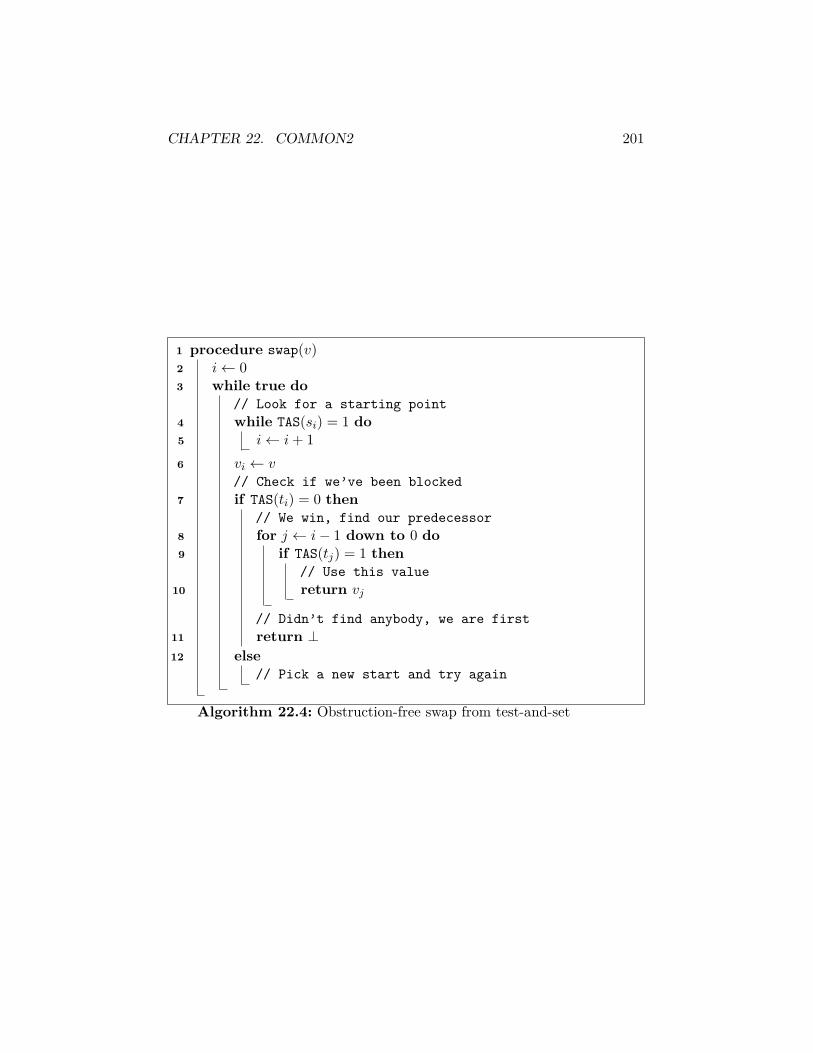
CHAPTER 22. COMMON2 201

1 procedure swap(v)2 i← 03 while true do

// Look for a starting point4 while TAS(si) = 1 do5 i← i+ 16 vi ← v

// Check if we’ve been blocked7 if TAS(ti) = 0 then

// We win, find our predecessor8 for j ← i− 1 down to 0 do9 if TAS(tj) = 1 then

// Use this value10 return vj

// Didn’t find anybody, we are first11 return ⊥12 else

// Pick a new start and try again

Algorithm 22.4: Obstruction-free swap from test-and-set

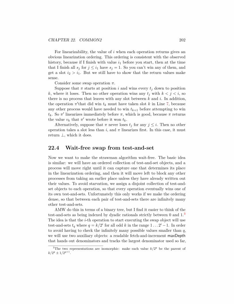
CHAPTER 22. COMMON2 202

For linearizability, the value of i when each operation returns gives anobvious linearization ordering. This ordering is consistent with the observedhistory, because if I finish with value i1 before you start, then at the timethat I finish all sj for j ≤ i1 have sj = 1. So you can’t win any of them, andget a slot i2 > i1. But we still have to show that the return values makesense.

Consider some swap operation π.Suppose that π starts at position i and wins every tj down to position

k, where it loses. Then no other operation wins any tj with k < j < i, sothere is no process that leaves with any slot between k and i. In addition,the operation π′that did win tk must have taken slot k in Line 7, becauseany other process would have needed to win tk+1 before attempting to wintk. So π′ linearizes immediately before π, which is good, because π returnsthe value vk that π′ wrote before it won tk.

Alternatively, suppose that π never loses tj for any j ≤ i. Then no otheroperation takes a slot less than i, and π linearizes first. In this case, it mustreturn ⊥, which it does.

22.4 Wait-free swap from test-and-setNow we want to make the strawman algorithm wait-free. The basic ideais similar: we will have an ordered collection of test-and-set objects, and aprocess will move right until it can capture one that determines its placein the linearization ordering, and then it will move left to block any otherprocesses from taking an earlier place unless they have already written outtheir values. To avoid starvation, we assign a disjoint collection of test-and-set objects to each operation, so that every operation eventually wins one ofits own test-and-sets. Unfortunately this only works if we make the orderingdense, so that between each pair of test-and-sets there are infinitely manyother test-and-sets.

AMW do this in terms of a binary tree, but I find it easier to think of thetest-and-sets as being indexed by dyadic rationals strictly between 0 and 1.3The idea is that the i-th operation to start executing the swap object will usetest-and-sets tq where q = k/2i for all odd k in the range 1 . . . 2i−1. In orderto avoid having to check the infinitely many possible values smaller than q,we will use two auxiliary objects: a readable fetch-and-increment maxDepththat hands out denominators and tracks the largest denominator used so far,

3The two representations are isomorphic: make each value k/2q be the parent ofk/2q ± 1/2q+1.

CHAPTER 22. COMMON2 203

and a max register accessed that keeps track of the largest position accessedso far.

AMW implement accessed using a snapshot, which we will do as well toavoid complications from trying to build a max register out of an infinitelydeep tree.4 Note that AMW don’t call this data structure a max register,but we will, because we like max registers.

Code for the swap procedure is given in Algorithm 22.5.To show Algorithm 22.5 works, we need the following technical lemma,

which, among other things, implies that node 1− 2depth is always availableto be captured by the process at depth depth. This is essentially just arestatement of Lemma 1 from [AMW11].

Lemma 22.4.1. For any x = k/2q, where k is odd, no process attempts tocapture any y ∈ [x, x+ 1/2q) before some process writes x to accessed.

Proof. Suppose that the lemma fails, let y = `/2r be the first node capturedin violation of the lemma, and let x = k/2q be such that y ∈ [x, x + 1/2q)but x has not been written to accessed when y is captured. Let p be theprocess that captures y.

Now consider y′ = x − 1/2r, the last node to the left of x at the samedepth as y. Why didn’t p capture y′?

One possibility is that some other process p′ blocked y′ during its returnphase. This p′ must have captured a node z > y′. If z > y, then p′ wouldhave blocked y first, preventing p from capturing it. So y′ < z < y.

The other possibility is that p never tried to capture y′, because someother process p′ wrote some value z > y′ to accessed first. This value z mustalso be less than y (or else p would not have tried to capture y).

In both cases, there is a process p′ that captures a value z with y′ < z < y,before p captures y and thus before anybody writes x to accessed.

Since y′ < x and y′ < z, either y′ < z < x or y′ < x < z. In the first case,z ∈ [y′, y′ + 1/2r) is captured before y′ is written to accessed. In the secondcase z ∈ [x, x + 1/2q) is captured before x is written to accessed. Eitherway, y is not the first capture to violate the lemma, contradicting our initialassumption.

Using Lemma 22.4.1, it is straightforward to show that Algorithm 22.5 iswait-free. If I get q for my value of depth, then no process will attempt to

4The issue is not so much that we can’t store arbitrary dyadics, since we can encode themusing an order-preserving prefix-free code, but that, without some sort of helping mechanism,a read running concurrently with endlessly increasing writes (e.g. 1/2, 3/4, 7/8, . . . ) mightnot be wait-free. Plus as soon as the denominator exceeds 2n, which happens after only ncalls to swap, O(n)-step snapshots are cheaper anyway.

CHAPTER 22. COMMON2 204

1 procedure swap(v)// Pick a new row just for me

2 depth← fetchAndIncrement(maxDepth)// Capture phase

3 repeat// Pick leftmost node in my row greater than

accessed4 cap← min

x∣∣∣ x = k/2depth for odd k, x > accessed

// Post my value

5 reg[cap]← v// Try to capture the test-and-set

6 win← TAS(tst[cap]) = 07 writeMax(accessed, cap)8 until win

// Return phase// Max depth reached by anybody left of cap

9 maxPreviousDepth← read(maxDepth)10 ret← cap

// Block previous nodes until we find one we can take11 repeat12 ret← max x = k/2q | q ≤ maxPreviousDepth, k odd, x < ret13 if ret < 0 then14 return ⊥15 until TAS(tst[ret]) = 116 return reg[ret]

Algorithm 22.5: Wait-free swap from test-and-set [AMW11]

CHAPTER 22. COMMON2 205

capture any y in [1− 2q, 1) before I write 1− 2q to accessed. But this meansthat nobody can block me from capturing 1− 2q, because processes can onlyblock values smaller than the one they already captured. I also can’t getstuck in the return phase, because there are only finitely many values withdenominator less than 2maxPreviousDepth.

It remains to show that the implementation is linearizable. The obviouslinearization ordering is given by sorting each operation i by its capturednode cap. Linearizability requires then that if we imagine a directed graphcontaining an edge ij for each pair of operations i and j such that i capturescapi and returns reg[capj ], then this graph forms a path that corresponds tothis linearization ordering.

Since each process only returns one value, it trivially holds that eachnode in the graph has out-degree at most 1. For the in-degree, suppose thatwe have operations i, j, and k with capi < capj < capk such that j and kboth return reg[capi]. Before k reaches tst[capi], it must first capture allthe test-and-sets between capi and capk that have depth less than or equalto maxPreviousDepthk. This will include tst[capj ], because j must write tomaxDepth before doing anything, and this must occur before k starts thereturn phase if j sees a value of accessed that is less that capk.

A similar argument show that there is at most one process that returns⊥; this implies that there is at most one process with out-degree 0.

So now we have a directed graph where every process has in-degree andout-degree at most one, which implies that each weakly-connected componentwill be a path. But each component will also have exactly one terminalnode with out-degree 0. Since there is only one such node, there is only onecomponent, and the entire graph is a single path. This concludes the proofof linearizability.

22.5 Implementations using stronger base objectsThe terrible step complexity of known wait-free implementations of Com-mon2 objects like swap or fetchAndIncrement from 2-process consensusobjects and registers has led to work on finding better implementationsassuming stronger base objects. Using load-linked/store-conditional, Ellenand Woelfel [EW13] provide implementations of several Common2 objects, in-cluding fetchAndIncrement, fetchAndAdd, and swap that all have O(logn)individual step complexity.5 This is know to be optimal due to a lower bound

5What they actually implement is the ability to do fetch-and-f , where f is any binaryassociative function, using an object they call an aggregator. Each of these objects is

CHAPTER 22. COMMON2 206

of Jayanti [Jay98].The lower bound applies a fortiori to the case where we don’t have

LL/SC or CAS and have to rely on 2-process consensus objects. But it’s notout of the question that there is a matching upper bound in this case.

obtained by choosing an appropriate f .

Chapter 23

Randomized consensus andtest-and-set

We’ve seen that we can’t solve consensus in an asynchronous system message-passing or shared-memory system with one crash failure [FLP85, LAA87],but that the problem becomes solvable using failure detectors [CT96]. Analternative that also allows us to solve consensus is to allow the processesto use randomization, by providing each process with a local coin that cangenerate random values that are immediately visible only to that process.The resulting randomized consensus problem replaces the terminationrequirement with probabilistic termination: all processes terminate withprobability 1. The agreement and validity requirements remain the same.

In this chapter, we will describe how randomization interacts with theadversary, give a bit of history of randomized consensus, and then concen-trate on recent algorithms for randomized consensus and the closely-relatedproblem of randomized test-and-set. Much of the material in this chapter isadapted from notes for a previous course on randomized algorithms [Asp11]and a few of my own papers [Asp12b, AE11, Asp12a].

23.1 Role of the adversary in randomized algo-rithms

Because randomized processes are unpredictable, we need to become alittle more sophisticated in our handling of the adversary. As in previousasynchronous protocols, we assume that the adversary has control overtiming, which we model by allowing the adversary to choose at each stepwhich process performs the next operation. But now the adversary may do

207

CHAPTER 23. RANDOMIZED CONSENSUS AND TEST-AND-SET208

so based on knowledge of the state of the protocol and its past evolution.How much knowledge we give the adversary affects its power. Several classesof adversaries have been considered in the literature; ranging from strongestto weakest, we have:

1. An adaptive adversary. This adversary is a function from the stateof the system to the set of processes; it can see everything that hashappened so far (including coin-flips internal to processes that have notyet been revealed to anybody else), but can’t predict the future. It’sknown that an adaptive adversary can force any randomized consensusprotocol to take Θ(n2) total steps [AC08]. The adaptive adversaryis also called a strong adversary following a foundational paper ofAbrahamson [Abr88].

2. An intermediate adversary or weak adversary [Abr88] is onethat limits the adversary’s ability to observe or control the systemin some way, without completely eliminating it. For example, acontent-oblivious adversary [Cha96] or value-oblivious adver-sary [Aum97] is restricted from seeing the values contained in registersor pending write operations and from observing the internal statesof processes directly. A location-oblivious adversary [Asp12b] candistinguish between values and the types of pending operations, butcan’t discriminate between pending operations based one which registerthey are operating on. These classes of adversaries are modeled byimposing an equivalence relation on partial executions and insistingthat the adversary make the same choice of processes to go next inequivalent situations. Typically they arise because somebody inventeda consensus protocol for the oblivious adversary (described below) andthen looked for the next most powerful adversary that still let theprotocol work.Weak adversaries often allow much faster consensus protocols thanadaptive adversaries. Each of the above adversaries permits consensusto be achieved in O(logn) expected individual work using an appropri-ate algorithm. But from a mathematical standpoint, weak adversariesare a bit messy, and once you start combining algorithms designed fordifferent weak adversaries, it’s natural to move all the way down to theweakest reasonable adversary, the oblivious adversary.

3. A oblivious adversary has no ability to observe the system at all;instead, it fixes a sequence of process ids in advance, and at each stepthe next process in the sequence runs.

CHAPTER 23. RANDOMIZED CONSENSUS AND TEST-AND-SET209

We will describe below a protocol that guarantees O(log logn) expectedindividual work for an oblivious adversary. It is not known whetherthis is optimal; in fact, is is consistent with the best known lower bound(due to Attiya and Censor [AC08]) that consensus can be solved inO(1) expected individual steps against an oblivious adversary.

Each of these adversaries is defined based on choosing steps of particularobjects, with particular constraints on knowledge based on the states of thoseobjects. This interacts badly with abstractions like linearizability: an adver-sary might be able to play games with the internals of an implementationof an object that allows it more power than it would have with an actualsequential version of the object. So even though linearizable implementationsare indistinguishable from sequential objects for deterministic protocols, forrandomized protocols they can give very different results for both adaptiveand oblivious adversaries [GHW11]; and in the specific case of consensus,it can be shown that there are randomized consensus protocols that termi-nate with probability 1 against an adaptive adversary when implementedwith atomic registers, but fail to terminate with nonzero probability whenimplemented using an arbitrary linearizable implementation [HHT20].

These results don’t necessarily imply the failure of any specific consensusprotocol implemented using a specific atomic register simulation, but theydo justify suspicion. The easiest way to deal with this suspicion is to assumethat our atomic registers are, in fact, atomic, so that’s what we will do here.

23.2 HistoryThe use of randomization to solve consensus in an asynchronous systemwith crash failures was proposed by Ben-Or [BO83] for a message-passingmodel. Chor, Israeli, and Li [CIL94] gave the first wait-free consensusprotocol for a shared-memory system, which assumed a particular kind ofweak adversary. Abrahamson [Abr88] defined strong and weak adversariesand gave the first wait-free consensus protocol for a strong adversary; itsexpected step complexity was Θ

(2n2). After failing to show that exponential

time was necessary, Aspnes and Herlihy [AH90a] showed how to do consensusin O(n4) total step complexity, a value that was soon reduced to O(n2 logn)by Bracha and Rachman [BR91]. This remained the best known bound forthe strong-adversary model until Attiya and Censor [AC08] showed matchingΘ(n2) upper and lower bounds on total step complexity. A later paper byAspnes and Censor [AC09] showed that it was also possible to get an O(n)bound on individual step complexity.

CHAPTER 23. RANDOMIZED CONSENSUS AND TEST-AND-SET210

For weak adversaries, the best known upper bound on individual stepcomplexity was O(logn) for a long time [Cha96, Aum97, Asp12b], withan O(n) bound on total step complexity for some models [Asp12b]. Morerecent work has lowered the bound to O(log logn), under the assumption ofan oblivious adversary [Asp12a]. No non-trivial lower bound on expectedindividual step complexity is known, although there is a known lower boundon the distribution of of the individual step complexity [ACH10].

In the following sections, we will concentrate on the more recent weak-adversary algorithms. These have the advantage of being fast enough thatone might reasonably consider using them in practice, assuming that theweak-adversary assumption does not create trouble, and they are also requireless probabilistic machinery to analyze than the strong-adversary algorithms.

23.3 Reduction to simpler primitivesTo show how to solve consensus using randomization, it helps to split theproblem in two: we will first see how to detect when we’ve achieved agreement,and then look at how to achieve agreement.

23.3.1 Adopt-commit objects

Most known randomized consensus protocols have a round-based structurethat alternates between generating and detecting agreement. Gafni [Gaf98]proposed adopt-commit protocols as a tool for detecting agreement, andthese protocols were later abstracted as adopt-commit objects [MRRT08,AGGT09]. The version described here is largely taken from [AE11], whichshows bounds on the complexity of adopt-commit objects.

An adopt-commit object supports a single operation, AdoptCommit (u),where u is an input from a set of m values. The result of this operation is anoutput of the form (commit, v) or (adopt, v), where the second component isa value from this set and the first component is a decision bit that indicateswhether the process should decide value v immediately or adopt it as itspreferred value in later rounds of the protocol.

The requirements for an adopt-commit object are the usual requirementsof validity and termination, plus:

1. Coherence. If the output of some operation is (commit, v), then everyoutput is either (adopt, v) or (commit, v).

2. Convergence. If all inputs are v, all outputs are (commit, v).

CHAPTER 23. RANDOMIZED CONSENSUS AND TEST-AND-SET211

These last two requirement replace the agreement property of consensus.They are also strictly weaker than consensus, which means that a consensusobject (with all its output labeled commit) is also an adopt-commit object.

The reason we like adopt-commit objects is that they allow the simpleconsensus protocol shown in Algorithm 23.1.

1 preference← input2 for r ← 1 . . .∞ do3 (b, preference)← AdoptCommit(AC[r], preference)4 if b = commit then5 return preference6 else7 do something to generate a new preference

Algorithm 23.1: Consensus using adopt-commit

The idea is that the adopt-commit takes care of ensuring that oncesomebody returns a value (after receiving commit), everybody else whodoesn’t return adopts the same value (follows from coherence). Conversely,if everybody already has the same value, everybody returns it (follows fromconvergence). The only missing piece is the part where we try to shake allthe processes into agreement. For this we need a separate object called aconciliator.

23.3.2 Conciliators

Conciliators are a weakened version of randomized consensus that replaceagreement with probabilistic agreement: the processes can disagree some-times, but must agree with constant probability despite interference by theadversary. An algorithm that satisfies termination, validity, and probabilisticagreement is called a conciliator.1

The important feature of conciliators is that if we plug a conciliator thatguarantees agreement with probability at least δ into Algorithm 23.1, thenon average we only have to execute the loop 1/δ times before every processagrees. This gives an expected cost equal to 1/δ times the total cost ofAdoptCommit and the conciliator. Typically we will aim for constant δ.

1Warning: This name has not really caught on in the general theory-of-distributed-computing community, and so far only appears in papers that have a particular researcheras a co-author [Asp12a, AE11, Asp12b, AACV17]. Unfortunately, there doesn’t seem tobe a better name for the same object that has caught on. So we are stuck with it for now.

CHAPTER 23. RANDOMIZED CONSENSUS AND TEST-AND-SET212

23.4 Implementing an adopt-commit objectWhat’s nice about adopt-commit objects is that they can be implementeddeterministically. Here we’ll give a simple adopt-commit object for two values,0 and 1. Optimal (under certain assumptions) constructions of m-valuedadopt-commits can be found in [AE11].

Pseudocode is given in Algorithm 23.2.

shared data: a[0], a[1], initially false; proposal, initially ⊥1 procedure AdoptCommit(v)2 a[v]← 13 if proposal = ⊥ then4 proposal← v5 else6 v ← proposal7 if a[¬v] = false then8 return (commit, v)9 else

10 return (adopt, v)

Algorithm 23.2: A 2-valued adopt-commit object

Structurally, this is pretty similar to a splitter (see §17.4.2), except thatwe use values instead of process ids.

We now show correctness. Termination and validity are trivial. Forcoherence, observe that if I return (commit, v) I must have read a[¬v] = falsebefore any process with ¬v writes a[¬v]; it follows that all such processeswill see proposal 6= ⊥ and return (adopt, v). For convergence, observe thatif all processes have the same input v, they all write it to proposal and allobserve a[¬v] = false, causing them all to return (commit, v).

23.5 Conciliators and shared coinsFor an adaptive adversary, the usual way to implement a conciliator isfrom a weak shared coin [AH90a], which is basically a non-cryptographicversion of the common coin [Rab83] found in many cryptographic Byzantineagreement protocols. Formally, a weak shared coin is an object that hasno inputs and returns either 0 or 1 to all processes with some minimumprobability δ. By itself this does not give validity, so converting a weak

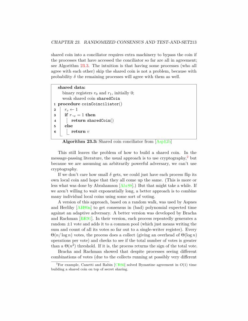
CHAPTER 23. RANDOMIZED CONSENSUS AND TEST-AND-SET213

shared coin into a conciliator requires extra machinery to bypass the coin ifthe processes that have accessed the conciliator so far are all in agreement;see Algorithm 23.3. The intuition is that having some processes (who allagree with each other) skip the shared coin is not a problem, because withprobability δ the remaining processes will agree with them as well.

shared data:binary registers r0 and r1, initially 0;weak shared coin sharedCoin

1 procedure coinCoinciliator()2 rv ← 13 if r¬v = 1 then4 return sharedCoin()5 else6 return v

Algorithm 23.3: Shared coin conciliator from [Asp12b]

This still leaves the problem of how to build a shared coin. In themessage-passing literature, the usual approach is to use cryptography,2 butbecause we are assuming an arbitrarily powerful adversary, we can’t usecryptography.

If we don’t care how small δ gets, we could just have each process flip itsown local coin and hope that they all come up the same. (This is more orless what was done by Abrahamson [Abr88].) But that might take a while. Ifwe aren’t willing to wait exponentially long, a better approach is to combinemany individual local coins using some sort of voting.

A version of this approach, based on a random walk, was used by Aspnesand Herlihy [AH90a] to get consensus in (bad) polynomial expected timeagainst an adaptive adversary. A better version was developed by Brachaand Rachman [BR91]. In their version, each process repeatedly generates arandom ±1 vote and adds it to a common pool (which just means writing thesum and count of all its votes so far out to a single-writer register). EveryΘ(n/ logn) votes, the process does a collect (giving an overhead of Θ(logn)operations per vote) and checks to see if the total number of votes is greaterthan a Θ(n2) threshold. If it is, the process returns the sign of the total vote.

Bracha and Rachman showed that despite processes seeing differentcombinations of votes (due to the collects running at possibly very different

2For example, Canetti and Rabin [CR93] solved Byzantine agreement in O(1) timebuilding a shared coin on top of secret sharing.

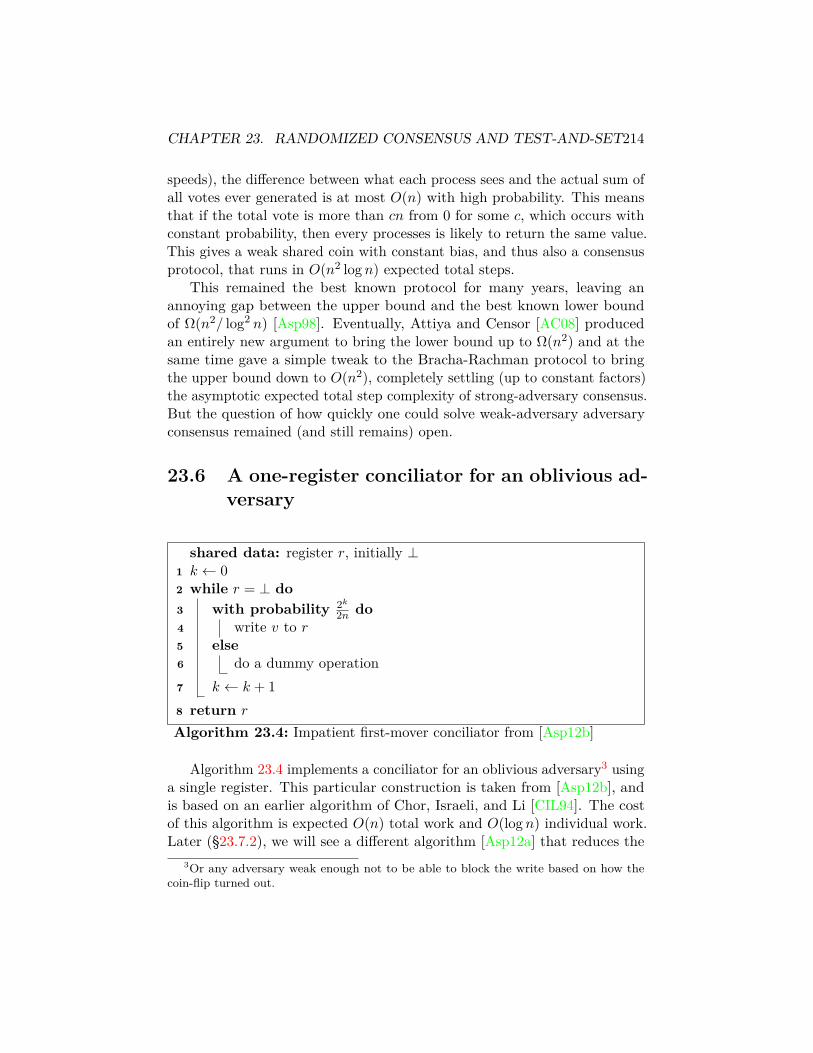
CHAPTER 23. RANDOMIZED CONSENSUS AND TEST-AND-SET214

speeds), the difference between what each process sees and the actual sum ofall votes ever generated is at most O(n) with high probability. This meansthat if the total vote is more than cn from 0 for some c, which occurs withconstant probability, then every processes is likely to return the same value.This gives a weak shared coin with constant bias, and thus also a consensusprotocol, that runs in O(n2 logn) expected total steps.

This remained the best known protocol for many years, leaving anannoying gap between the upper bound and the best known lower boundof Ω(n2/ log2 n) [Asp98]. Eventually, Attiya and Censor [AC08] producedan entirely new argument to bring the lower bound up to Ω(n2) and at thesame time gave a simple tweak to the Bracha-Rachman protocol to bringthe upper bound down to O(n2), completely settling (up to constant factors)the asymptotic expected total step complexity of strong-adversary consensus.But the question of how quickly one could solve weak-adversary adversaryconsensus remained (and still remains) open.

23.6 A one-register conciliator for an oblivious ad-versary

shared data: register r, initially ⊥1 k ← 02 while r = ⊥ do3 with probability 2k

2n do4 write v to r5 else6 do a dummy operation7 k ← k + 18 return r

Algorithm 23.4: Impatient first-mover conciliator from [Asp12b]

Algorithm 23.4 implements a conciliator for an oblivious adversary3 usinga single register. This particular construction is taken from [Asp12b], andis based on an earlier algorithm of Chor, Israeli, and Li [CIL94]. The costof this algorithm is expected O(n) total work and O(logn) individual work.Later (§23.7.2), we will see a different algorithm [Asp12a] that reduces the

3Or any adversary weak enough not to be able to block the write based on how thecoin-flip turned out.

CHAPTER 23. RANDOMIZED CONSENSUS AND TEST-AND-SET215

individual work to O(log logn), although the total work for that algorithmmay be O(n log logn).

The basic idea is that processes alternate between reading a register rand (maybe) writing to the register; if a process reads a non-null value fromthe register, it returns it. Any other process that reads the same non-nullvalue will agree with the first process; the only way that this can’t happen isif some process writes a different value to the register before it notices thefirst write.

The random choice of whether to write the register or not avoids thisproblem. The idea is that even though the adversary can schedule a write ata particular time, because it’s oblivious, it won’t be able to tell if the processwrote (or was about to write) or did a no-op instead.

The basic version of this algorithm, due to Chor, Israeli, and Li [CIL94],uses a fixed 1

2n probability of writing to the register. So once some processwrites to the register, the chance that any of the remaining n− 1 processeswrite to it before noticing that it’s non-null is at most n−1

2n < 1/2. It’s alsonot hard to see that this algorithm uses O(n) total operations, although itmay be that one single process running by itself has to go through the loop2n times before it finally writes the register and escapes.

Using increasing probabilities avoids this problem, because any processthat executes the main loop dlgne + 1 times will write the register. Thisestablishes the O(logn) per-process bound on operations. At the same time,an O(n) bound on total operations still holds, since each write has at leasta 1

2n chance of succeeding. The price we pay for the improvement is thatwe increase the chance that an initial value written to the register getsoverwritten by some high-probability write. But the intuition is that theprobabilities can’t grow too much, because the probability that I write onmy next write is close to the sum of the probabilities that I wrote on myprevious writes—suggesting that if I have a high probability of writing nexttime, I should have done a write already.

Formalizing this intuition requires a little bit of work. Fix the schedule,and let pi be the probability that the i-th write operation in this schedulesucceeds. Let t be the least value for which

∑ti=1 pi ≥ 1/4. We’re going to

argue that with constant probability one of the first t writes succeeds, andthat the next n− 1 writes by different processes all fail.

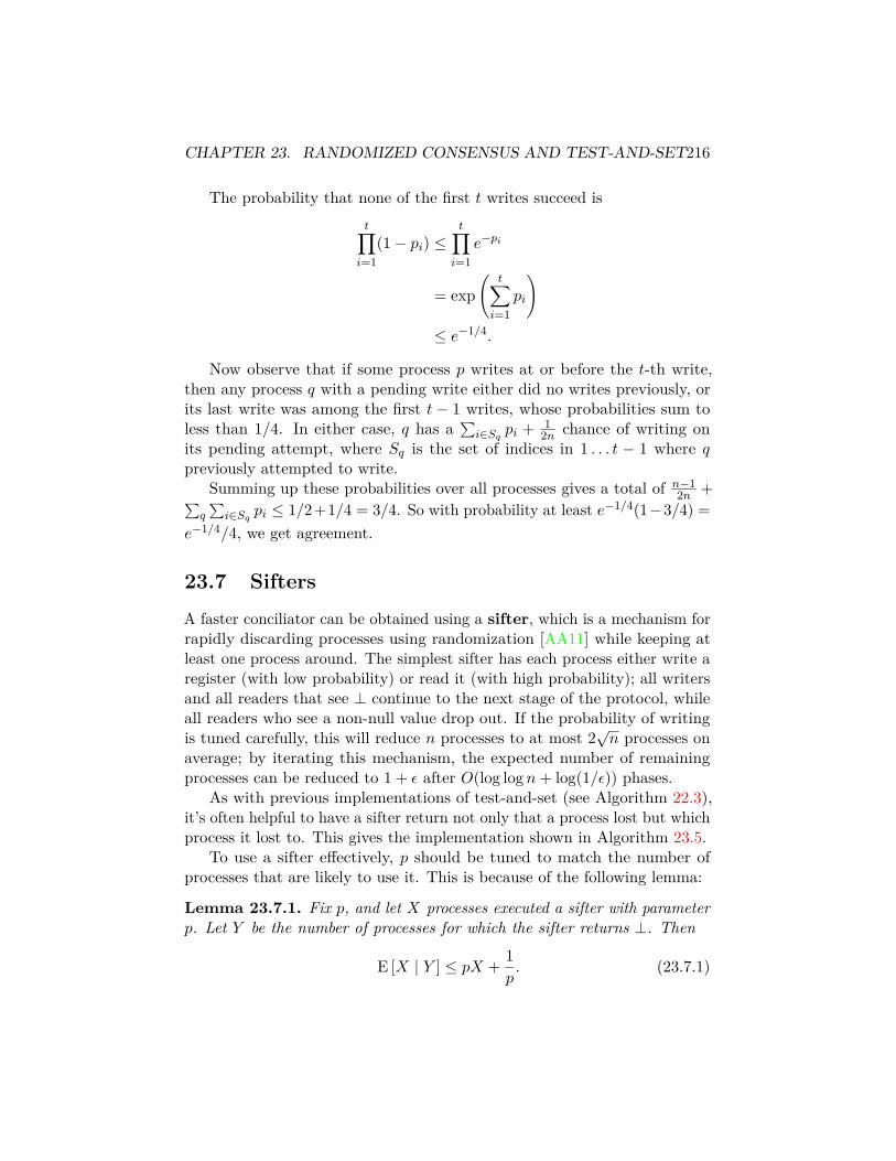
CHAPTER 23. RANDOMIZED CONSENSUS AND TEST-AND-SET216

The probability that none of the first t writes succeed ist∏i=1

(1− pi) ≤t∏i=1

e−pi

= exp(

t∑i=1

pi

)≤ e−1/4.

Now observe that if some process p writes at or before the t-th write,then any process q with a pending write either did no writes previously, orits last write was among the first t − 1 writes, whose probabilities sum toless than 1/4. In either case, q has a

∑i∈Sq pi + 1

2n chance of writing onits pending attempt, where Sq is the set of indices in 1 . . . t − 1 where qpreviously attempted to write.

Summing up these probabilities over all processes gives a total of n−12n +∑

q

∑i∈Sq pi ≤ 1/2+1/4 = 3/4. So with probability at least e−1/4(1−3/4) =

e−1/4/4, we get agreement.

23.7 SiftersA faster conciliator can be obtained using a sifter, which is a mechanism forrapidly discarding processes using randomization [AA11] while keeping atleast one process around. The simplest sifter has each process either write aregister (with low probability) or read it (with high probability); all writersand all readers that see ⊥ continue to the next stage of the protocol, whileall readers who see a non-null value drop out. If the probability of writingis tuned carefully, this will reduce n processes to at most 2

√n processes on

average; by iterating this mechanism, the expected number of remainingprocesses can be reduced to 1 + ε after O(log logn+ log(1/ε)) phases.

As with previous implementations of test-and-set (see Algorithm 22.3),it’s often helpful to have a sifter return not only that a process lost but whichprocess it lost to. This gives the implementation shown in Algorithm 23.5.

To use a sifter effectively, p should be tuned to match the number ofprocesses that are likely to use it. This is because of the following lemma:

Lemma 23.7.1. Fix p, and let X processes executed a sifter with parameterp. Let Y be the number of processes for which the sifter returns ⊥. Then

E [X | Y ] ≤ pX + 1p. (23.7.1)

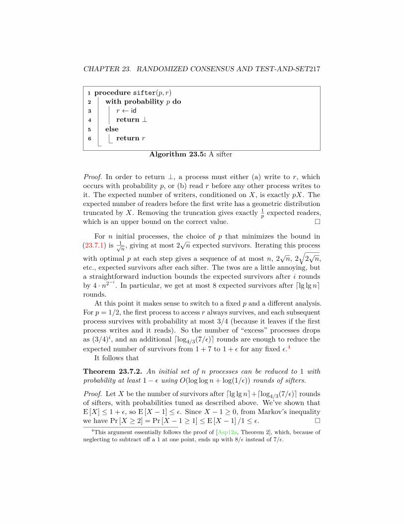
CHAPTER 23. RANDOMIZED CONSENSUS AND TEST-AND-SET217

1 procedure sifter(p, r)2 with probability p do3 r ← id4 return ⊥5 else6 return r

Algorithm 23.5: A sifter

Proof. In order to return ⊥, a process must either (a) write to r, whichoccurs with probability p, or (b) read r before any other process writes toit. The expected number of writers, conditioned on X, is exactly pX. Theexpected number of readers before the first write has a geometric distributiontruncated by X. Removing the truncation gives exactly 1

p expected readers,which is an upper bound on the correct value.

For n initial processes, the choice of p that minimizes the bound in(23.7.1) is 1√

n, giving at most 2

√n expected survivors. Iterating this process

with optimal p at each step gives a sequence of at most n, 2√n, 2

√2√n,

etc., expected survivors after each sifter. The twos are a little annoying, buta straightforward induction bounds the expected survivors after i roundsby 4 · n2−i . In particular, we get at most 8 expected survivors after dlg lgnerounds.

At this point it makes sense to switch to a fixed p and a different analysis.For p = 1/2, the first process to access r always survives, and each subsequentprocess survives with probability at most 3/4 (because it leaves if the firstprocess writes and it reads). So the number of “excess” processes dropsas (3/4)i, and an additional dlog4/3(7/ε)e rounds are enough to reduce theexpected number of survivors from 1 + 7 to 1 + ε for any fixed ε.4

It follows that

Theorem 23.7.2. An initial set of n processes can be reduced to 1 withprobability at least 1− ε using O(log logn+ log(1/ε)) rounds of sifters.

Proof. Let X be the number of survivors after dlg lgne+dlog4/3(7/ε)e roundsof sifters, with probabilities tuned as described above. We’ve shown thatE [X] ≤ 1 + ε, so E [X − 1] ≤ ε. Since X − 1 ≥ 0, from Markov’s inequalitywe have Pr [X ≥ 2] = Pr [X − 1 ≥ 1] ≤ E [X − 1] /1 ≤ ε.

4This argument essentially follows the proof of [Asp12a, Theorem 2], which, because ofneglecting to subtract off a 1 at one point, ends up with 8/ε instead of 7/ε.

CHAPTER 23. RANDOMIZED CONSENSUS AND TEST-AND-SET218

23.7.1 Test-and-set using sifters

Sifters were initially designed to be used for test-and-set. For this purpose,we treat a return value of ⊥ as “keep going” and anything else as “leave withvalue 1.” Using O(log logn) rounds of sifters, we can get down to one processthat hasn’t left with probability at least 1− log−c n for any fixed constantc. We then need a fall-back TAS to handle the log−c n chance that we getmore than one such survivor.

Alistarh and Aspnes [AA11] used the RatRace algorithm of Alistarh etal. [AAG+10] for this purpose. This is an adaptive randomized test-and-setbuilt from splitters and two-process consensus objects that runs in O(log k)expected time, where k is the number of processes that access the test-and-set;a sketch of this algorithm is given in §24.5.2. If we want to avoid appealingto this algorithm, a somewhat simpler approach is to use an approach similarto the Lamport’s fast-path mutual exclusion algorithm (described in §17.4.2):any process that survives the sifters tries to rush to a two-process TAS at thetop of a tree of two-processes TASes by winning a splitter, and if it doesn’twin the splitter, it enters at a leaf and pays O(logn) expected steps. Bysetting ε = 1/ logn, the overall expected cost of this final stage is O(1).

This algorithm does not guarantee linearizability. I might lose a sifterearly on only to have a later process win all the sifters (say, by writing toeach one) and return 0. A gate bit as in Algorithm 22.3 solves this problem.The full code is given in Algorithm 23.6.

23.7.2 Consensus using sifters

With some trickery, the sifter mechanism can be adapted to solve consensus,still in O(log logn) expected individual work [Asp12a]. The main difficultyis that a process can no longer drop out as soon as it knows that it lost: itstill needs to figure out who won, and possible help that winner over thefinish line.

The basic idea is that when a process p loses a sifter to some other processq, p will act like a clone of q from that point on. In order to make this work,each process writes down at the start of the protocol all of the coin-flips itintends to use to decide whether to read or write at each round of sifting.Together with its input, these coin-flips make up the process’s persona.In analyzing the progress of the sifter, we count surviving personae (withmultiple copies of the same persona counting as one) instead of survivingprocesses.

Pseudocode for this algorithm is given in Algorithm 23.7. Note that the

CHAPTER 23. RANDOMIZED CONSENSUS AND TEST-AND-SET219

1 if gate 6= ⊥ then2 return 13 else4 gate← myId5 for i← 1 . . . dlog logne+ dlog4/3(7 logn)e do6 with probability min

(1/2, 21−2−i+1

)do

7 ri ← myId8 else9 w ← ri

10 if w 6= ⊥ then11 return 1

12 if splitter() = stop then13 return 014 else15 return AWWTAS()

Algorithm 23.6: Test-and-set in O(log logn) expected time

loop body is essentially the same as the code in Algorithm 23.5, except thatthe random choice is replaced by a lookup in persona.chooseWrite.

To show that this works, we need to argue that having multiple copiesof a persona around doesn’t change the behavior of the sifter. In eachround, we will call the first process with a given persona p to access rithe representative of p, and argue that a persona survives round i inthis algorithm precisely when its representative would survive round i ina corresponding test-and-set sifter with the schedule restricted only to therepresentatives.

There are three cases:

1. The representative of p writes. Then at least one copy of p survives.

2. The representative of p reads a null value. Again at least one copy ofp survives.

3. The representative of p reads a non-null value. Then no copy of psurvives: all subsequent reads by processes carrying p also read anon-null value and discard p, and since no process with p writes, noother process adopts p.

CHAPTER 23. RANDOMIZED CONSENSUS AND TEST-AND-SET220

1 procedure conciliator(input)2 Let R = dlog logne+ dlog4/3(7/ε)e3 Let chooseWrite be a vector of R independent random Boolean

variables with Pr[chooseWrite[i] = 1] = pi, wherepi = 21−2−i+1(n)−2−i for i ≤ dlog logne and pi = 1/2 for larger i.

4 persona← 〈input, chooseWrite,myId〉5 for i← 1 . . . R do6 if persona.chooseWrite[i] = 1 then7 ri ← persona8 else9 v ← ri

10 if v 6= ⊥ then11 persona← v

12 return persona.input

Algorithm 23.7: Sifting conciliator (from [Asp12a])

From the preceding analysis for test-and-set, we have that afterO(log logn+log 1/ε) rounds with appropriate probabilities of writing, at most 1 + ε valuessurvive on average. This gives a probability of at most ε of disagreement. Byalternating these conciliators with adopt-commit objects, we get agreementin O(log logn+ logm/ log logm) expected time, where m is the number ofpossible input values.

I don’t think the O(log logn) part of this expression is optimal, but Idon’t know how to do better.

23.7.3 A better sifter for test-and-set

A more sophisticated sifter due to Giakkoupis and Woelfel [GW12a] removesall but O(logn) processes, on average, using two operations for each process.Iterating this sifter reduces the expected survivors to O(1) in O(log∗ n)rounds. A particularly nice feature of the Giakkoupis-Woelfel algorithm isthat (if you don’t care about space) it doesn’t have any parameters thatrequire tuning to n: this means that exactly the same structure can be usedin each round. An unfortunate feature is that it’s not possible to guaranteethat every process that leaves learns the identity of a process that stays: thismeans that it can’t adapted into a consensus protocol using the persona trick

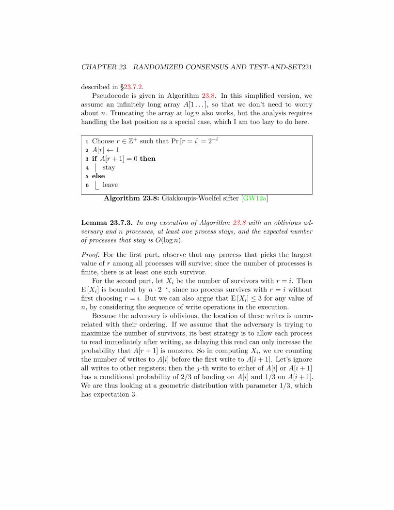
CHAPTER 23. RANDOMIZED CONSENSUS AND TEST-AND-SET221

described in §23.7.2.Pseudocode is given in Algorithm 23.8. In this simplified version, we

assume an infinitely long array A[1 . . . ], so that we don’t need to worryabout n. Truncating the array at logn also works, but the analysis requireshandling the last position as a special case, which I am too lazy to do here.

1 Choose r ∈ Z+ such that Pr [r = i] = 2−i2 A[r]← 13 if A[r + 1] = 0 then4 stay5 else6 leave

Algorithm 23.8: Giakkoupis-Woelfel sifter [GW12a]

Lemma 23.7.3. In any execution of Algorithm 23.8 with an oblivious ad-versary and n processes, at least one process stays, and the expected numberof processes that stay is O(logn).

Proof. For the first part, observe that any process that picks the largestvalue of r among all processes will survive; since the number of processes isfinite, there is at least one such survivor.

For the second part, let Xi be the number of survivors with r = i. ThenE [Xi] is bounded by n · 2−i, since no process survives with r = i withoutfirst choosing r = i. But we can also argue that E [Xi] ≤ 3 for any value ofn, by considering the sequence of write operations in the execution.

Because the adversary is oblivious, the location of these writes is uncor-related with their ordering. If we assume that the adversary is trying tomaximize the number of survivors, its best strategy is to allow each processto read immediately after writing, as delaying this read can only increase theprobability that A[r + 1] is nonzero. So in computing Xi, we are countingthe number of writes to A[i] before the first write to A[i+ 1]. Let’s ignoreall writes to other registers; then the j-th write to either of A[i] or A[i+ 1]has a conditional probability of 2/3 of landing on A[i] and 1/3 on A[i+ 1].We are thus looking at a geometric distribution with parameter 1/3, whichhas expectation 3.

CHAPTER 23. RANDOMIZED CONSENSUS AND TEST-AND-SET222

Combining these two bounds gives E [Xi] ≤ min(3, 2−i). So then

E [survivors] ≤∞∑i=1

min(3, n · 2−i)

= 3 lgn+O(1),

because once n · 2−i drops below 3, the remaining terms form a geometricseries.

Like square root, logarithm is concave, so Jensen’s inequality applies hereas well. So O(log∗ n) rounds of Algorithm 23.8 reduces us to an expectedconstant number of survivors, which can then be fed to RatRace.

With an adaptive adversary, all of the sifter-based test-and-sets fail badly:in this particular case, an adaptive adversary can sort the processes in orderof increasing write location so that every process survives. The best knownn-process test-and-set for an adaptive adversary is still a tree of 2-processrandomized test-and-sets, as in the Afek et al. [AWW93] algorithm describedin §22.2. Whether O(logn) expected steps is in fact necessary is still open(as is the exact complexity of test-and-set with an oblivious adversary).

23.8 Space boundsA classic result of Fich, Herlihy, and Shavit [FHS98] showed that Ω(

√n)

registers are needed to solve consensus even under the very weak require-ment of nondeterministic solo termination, which says that for everyreachable configuration and every process p, there exists some continuationof the execution in which the protocol terminates with only p running. Thebest known upper bound is the trivial bound of n—one single-writer registerper process—since any algorithm that uses multi-writer registers can betranslated into one that uses only single-writer registers, and (assuming wideenough registers) multiple registers of a single process can be combined intoone.

For many years, there was very little progress in closing the gap betweenthese two bounds. In 2013, we got a hint that FHS might be tight whenGiakkoupis et al. [GHHW13] gave a surprising O(

√n)-space algorithm for

the closely related problem of obstruction-free one-shot test-and-set.But then Gelashvili [Gel15] showed an n/20 space lower bound for con-

sensus for anonymous processes, and Zhu quickly followed this with a lowerbound for non-anonymous processes [Zhu16], showing that at least n − 1registers are required, using a clever combination of bivalence and covering

CHAPTER 23. RANDOMIZED CONSENSUS AND TEST-AND-SET223

arguments. Around the same time, Giakkoupis et al. [GHHW15] furtherimproved the space complexity of obstruction-free test-and-set to O(logn),using a deterministic obstruction-free implementation of a sifter. So the briefcoincidence of the Ω(

√n) lower bound on consensus and the O(

√n) upper

bound on test-and-set turned out to be an accident.For consensus, there is still a gap, but it’s a very small gap. Whether

the actual space needed is n− 1 or n remains open.

Chapter 24

Renaming

We will start by following the presentation in [AW04, §16.3]. This mostlydescribes results of the original paper of Attiya et al. [ABND+90] that definedthe renaming problem and gave a solution for message-passing; however, it’snow more common to treat renaming in the context of shared-memory, so wewill follow Attiya and Welch’s translation of these results to a shared-memorysetting.

24.1 RenamingIn the renaming problem, we have n processes, each starts with a namefrom some huge namespace, and we’d like to assign them each unique namesfrom a much smaller namespace. The main application is allowing us to runalgorithms that assume that the processes are given contiguous numbers,e.g., the various collect or atomic snapshot algorithms in which each processis assigned a unique register and we have to read all of the registers. Withrenaming, instead of reading a huge pile of registers in order to find the fewthat are actually used, we can map the processes down to a much smallerset.

Formally, we have a decision problem where each process has input xi(its original name) and output yi, with the requirements:

Termination Every nonfaulty process eventually decides.

Uniqueness If pi 6= pj , then yi 6= yj .

Anonymity The code executed by any process depends only on its inputxi: for any execution of processes p1 . . . pn with inputs x1 . . . xn, and

224

CHAPTER 24. RENAMING 225

any permutation π of [1 . . . n], there is a corresponding execution ofprocesses pπ(1) . . . pπ(n) with inputs x1 . . . xn in which pπ(i) performsexactly the same operations as pi and obtains the same output yi.

The last condition is like non-triviality for consensus: it excludes algo-rithms where pi just returns i in all executions. Typically we do not haveto do much to prove anonymity other than observing that all processes arerunning the same code.

We will be considering renaming in a shared-memory system, where weonly have atomic registers to work with.

24.2 PerformanceConventions on counting processes:

• N = number of possible original names.

• n = maximum number of processes.

• k = number of processes that actually execute the algorithm.

Ideally, we’d like any performance measures we get to depend on k aloneif possible (giving an adaptive algorithm). Next best would be somethingpolynomial in n and k. Anything involving N is bad.

We’d also like to minimize the size of the output namespace. How wellwe can do this depends on what assumptions we make. For deterministicalgorithms using only read-write registers, a lower bound due to Herlihy andShavit [HS99] shows that we can’t get fewer than 2n− 1 names for generaln.1 Our target thus will be exactly 2n− 1 output names if possible, or 2k− 1if we are trying to be adaptive. For randomized algorithms, it is possible tosolve strong or tight renaming, where the size of the namespace is exactlyk; we’ll see how to do this in §24.5.

A small note on bounds: There is a lot of variation in the literature onhow bounds on the size of the output namespace are stated. The originalHerlihy-Shavit lower bound [HS99] says that there is no general renamingalgorithm that uses 2n names for n + 1 processes; in other words, any n-process algorithm uses at least 2n − 1 names. Many subsequent papers

1This lower bound was further refined by Castañeda and Rajsbaum [CR08], who showthat 2n − 2 (but no less!) is possible for certain special values of n; all of these lowerbounds make extensive use of combinatorial topology, so we won’t try to present themhere.

CHAPTER 24. RENAMING 226

discussing lower bounds on the namespace follow the approach of Herlihy andShavit and quote lower bounds that are generally 2 higher than the minimumnumber of names needed for n processes. This requires a certain amount oftranslation when comparing these lower bounds with upper bounds, whichuse the more natural convention.

24.3 Order-preserving renamingBefore we jump into upper bounds, let’s do an easy lower bound fromthe Attiya et al. paper [ABND+90]. This bound works on a variant ofrenaming called order-preserving renaming, where we require that yi <yj whenever xi < xj . Unfortunately, this requires a very large outputnamespace: with t failures, any asynchronous algorithm for order-preservingrenaming requires 2t(n− t+ 1)− 1 possible output names. This lower boundapplies regardless of the model, as long as some processes may start afterother processes have already been assigned names.

For the wait-free case, we have t = n− 1, and the bound becomes just2n−1. This is a simpler case than the general t-failure case, but the essentialidea is the same: if I’ve only seen a few of the processes, I need to leave roomfor the others.

Theorem 24.3.1. There is no order-preserving renaming algorithm for nprocesses using fewer than 2n − 1 names.

Proof. By induction on n. For n = 1, we use 21 − 1 = 1 names; this is thebase case. For larger n, suppose we use m names, and consider an executionin which one process pn runs to completion first. This consumes one nameyn and leaves k names less than yn and m− k− 1 names greater than yn. Bysetting all the inputs xi for i < n either less than xn or greater than xn, wecan force the remaining processes to choose from the remaining k or m−k−1names. Applying the induction hypothesis, this gives k ≥ 2n−1 − 1 andm−k−1 ≥ 2n−1−1, som = k+(m−k−1)+1 ≥ 2(2n−1−1)+1 = 2n−1.

24.4 Deterministic renamingIn deterministic renaming, we can’t use randomization, and may or maynot have any primitives stronger than atomic registers. With just atomicregisters, we can only solve loose renaming; with test-and-set, we can solvetight renaming. In this section, we describe some basic algorithms fordeterministic renaming.

CHAPTER 24. RENAMING 227

24.4.1 Wait-free renaming with 2n− 1 names

Here we use Algorithm 55 from [AW04], which is an adaptation to sharedmemory of the message-passing renaming algorithm of [ABND+90]. One oddfeature of the algorithm is that, as written, it is not anonymous: processescommunicate using an atomic snapshot object and use their process ids toselect which component of the snapshot array to write to. But if we think ofthe process ids used in the algorithm as the inputs xi rather than the actualprocess ids i, then everything works. The version given in Algorithm 24.1makes this substitution explicit, by treating the original name i as the input.

1 procedure getName()2 s← 13 while true do4 a[i]← s5 view← snapshot(a)6 if view[j] = s for some j then7 r ← |j : view[j] 6= ⊥ ∧ j ≤ i|8 s← r-th positive integer not in

view[j] : j 6= i ∧ view[j] = ⊥9 else

10 return s

Algorithm 24.1: Wait-free deterministic renaming

The array a holds proposed names for each process (indexed by theoriginal names), or ⊥ for processes that have not proposed a name yet. If aprocess proposes a name and finds that no other process has proposed thesame name, it takes it; otherwise it chooses a new name by first computingits rank r among the active processes and then choosing the r-th smallestname that hasn’t been proposed by another process. Because the rank is atmost n and there are at most n− 1 names proposed by the other processes,this always gives proposed names in the range [1 . . . 2n− 1]. But it remainsto show that the algorithm satisfies uniqueness and termination.

For uniqueness, consider two process with original names i and j. Supposethat i and j both decide on s. Then i sees a view in which a[i] = s anda[j] 6= s, after which it no longer updates a[i]. Similarly, j sees a view inwhich a[j] = s and a[i] 6= s, after which it no longer updates a[j]. If i’s viewis obtained first, then j can’t see a[i] 6= s, but the same holds if j’s view isobtained first. So in either case we get a contradiction, proving uniqueness.

CHAPTER 24. RENAMING 228

Termination is a bit trickier. Here we argue that no process can runforever without picking a name, by showing that if we have a set of processesthat are doing this, the one with smallest original name eventually picks aname. More formally, call a process trying if it runs for infinitely many stepswithout choosing a name. Then in any execution with at least one tryingprocess, eventually we reach a configuration where all processes have eitherfinished or are trying. In some subsequent configuration, all the processeshave written to the a array at least once; from this point on, the set of non-null positions in a—and thus the rank each process computes for itself—isstable.

Starting from some such stable configuration, look at the trying processi with the smallest original name, and suppose it has rank r. Let F =z1 < z2 . . . be the set of “free names” that are not proposed in a by anyof the finished processes. Observe that no trying process j 6= i ever proposesa name in z1 . . . zr, because any such process has rank greater than r.This leaves zr open for i to claim, provided the other names in z1 . . . zreventually become free. But this will happen, because only trying processesmay have proposed these names (early on in the execution, when the finishedprocesses hadn’t finished yet), and the trying processes eventually proposenew names that are not in this range. So eventually process i proposes zr,sees no conflict, and finishes, contradicting the assumption that it is trying.

Note that we haven’t proved any complexity bounds on this algorithm atall, but we know that the snapshot alone takes at least Ω(N) time and space.Brodksy et al. [BEW11] cite a paper of Bar-Noy and Dolev [BND89] as givinga shared-memory version of [ABND+90] with complexity O(n · 4n); they alsogive algorithms and pointers to algorithms with much better complexity.

24.4.2 Long-lived renaming

In long-lived renaming a process can release a name for later use by otherprocesses (or the same process, if it happens to run choose-name again).Now the bound on the number of names needed is 2k − 1, where k is themaximum number of concurrently active processes. Algorithm 24.1 can beconverted to a long-lived renaming algorithm by adding the releaseNameprocedure given in Algorithm 24.2. This just erases the process’s proposedname, so that some other process can claim it.

Here the termination requirement is weakened slightly, to say that someprocess always makes progress in getName. It may be, however, that thereis some process that never successfully obtains a name, because it keepsgetting stepped on by other processes zipping in and out of getName and

CHAPTER 24. RENAMING 229

1 procedure releaseName()2 a[i]← ⊥

Algorithm 24.2: Releasing a name

releaseName.

24.4.3 Renaming without snapshots

Moir and Anderson [MA95] give a renaming protocol that is somewhat easierto understand and doesn’t require taking snapshots over huge arrays. Adownside is that the basic version requires k(k + 1)/2 names to handle kactive processes.

24.4.3.1 Splitters

The Moir-Anderson renaming protocol uses a network of splitters, whichwe last saw providing a fast path for mutual exclusion in §17.4.2. Eachsplitter is a widget, built from a pair of atomic registers, that assigns toeach processes that arrives at it the value right, down, or stop. As discussedpreviously, the useful properties of splitters are that if at least one processarrives at a splitter, then (a) at least one process returns right or stop; and(b) at least one process returns down or stop; (c) at most one process returnsstop; and (d) any process that runs by itself returns stop.

We proved the last two properties in §17.4.2; we’ll prove the first two here.Another way of describing these properties is that of all the processes thatarrive at a splitter, some process doesn’t go down and some process doesn’tgo right. By arranging splitters in a grid, this property guarantees that everyrow or column that gets at least one process gets to keep it—which meansthat with k processes, no process reaches row k + 1 or column k + 1.

Algorithm 24.3 gives the implementation of a splitter (it’s identical toAlgorithm 17.5, but it will be convenient to have another copy here).

Lemma 24.4.1. If at least one process completes the splitter, at least oneprocess returns stop or right.

Proof. Suppose no process returns right; then every process sees open in door,which means that every process writes its id to race before any process closesthe door. Some process writes its id last: this process will see its own id inrace and return stop.

CHAPTER 24. RENAMING 230

shared data:1 atomic register race, big enough to hold an id, initially ⊥2 atomic register door, big enough to hold a bit, initially open3 procedure splitter(id)4 race← id5 if door = closed then6 return right7 door← closed8 if race = id then9 return stop

10 else11 return down

Algorithm 24.3: Implementation of a splitter

Lemma 24.4.2. If at least one process completes the splitter, at least oneprocess returns stop or down.

Proof. First observe that if no process ever writes to door, then no processcompletes the splitter, because the only way a process can finish the splitterwithout writing to door is if it sees closed when it reads door (which musthave been written by some other process). So if at least one process finishes,at least one process writes to door. Let p be any such process. From thecode, having written door, it has already passed up the chance to returnright; thus it either returns stop or down.

24.4.3.2 Splitters in a grid

Now build an m-by-m triangular grid of splitters, arranged as rows 0 . . .m−1and columns 0 . . .m− 1, where a splitter appears in each position (r, c) withr+c ≤ m−1 (see Figure 24.1 for an example; this figure is taken from [Asp10]).Assign a distinct name to each of the

(m2)splitters in this grid. To obtain

a name, a process starts at (r, c) = (0, 0), and repeatedly executes thesplitter at its current position (r, c). If the splitter returns right, it movesto (r, c+ 1); if down, it moves to (r + 1, c); if stop, it stops, and returns thename of its current splitter. This gives each name to at most one process(by Lemma 17.4.3); we also have to show that if at most m processes enterthe grid, every process stops at some splitter.

The argument for this is simple. Suppose some process p leaves thegrid on one of the 2m output wires. Look at the path it takes to get there

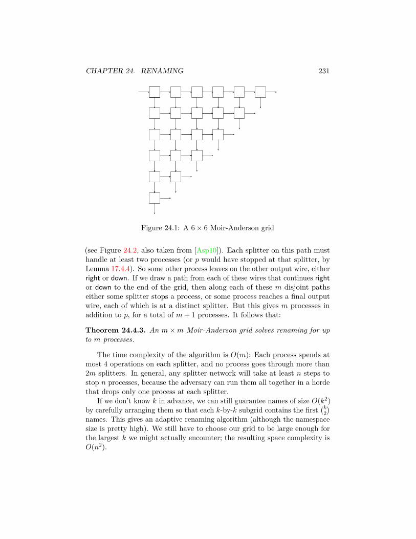
CHAPTER 24. RENAMING 231

Figure 24.1: A 6× 6 Moir-Anderson grid

(see Figure 24.2, also taken from [Asp10]). Each splitter on this path musthandle at least two processes (or p would have stopped at that splitter, byLemma 17.4.4). So some other process leaves on the other output wire, eitherright or down. If we draw a path from each of these wires that continues rightor down to the end of the grid, then along each of these m disjoint pathseither some splitter stops a process, or some process reaches a final outputwire, each of which is at a distinct splitter. But this gives m processes inaddition to p, for a total of m+ 1 processes. It follows that:

Theorem 24.4.3. An m×m Moir-Anderson grid solves renaming for upto m processes.

The time complexity of the algorithm is O(m): Each process spends atmost 4 operations on each splitter, and no process goes through more than2m splitters. In general, any splitter network will take at least n steps tostop n processes, because the adversary can run them all together in a hordethat drops only one process at each splitter.

If we don’t know k in advance, we can still guarantee names of size O(k2)by carefully arranging them so that each k-by-k subgrid contains the first

(k2)

names. This gives an adaptive renaming algorithm (although the namespacesize is pretty high). We still have to choose our grid to be large enough forthe largest k we might actually encounter; the resulting space complexity isO(n2).

CHAPTER 24. RENAMING 232

Figure 24.2: Path taken by a single process through a 6× 6 Moir-Andersongrid (heavy path), and the 6 disjoint paths it spawns (dashed paths).(From [Asp10].)

With a slightly more clever arrangement of the splitters, it is possible toreduce the space complexity to O(n3/2) [Asp10]. Whether further reductionsare possible is an open problem. Note however that linear time complexitymakes splitter networks uncompetitive with much faster randomized algo-rithms (as we’ll see in §24.5), so this may not be a very important openproblem.

24.4.4 Getting to 2n− 1 names in polynomial space

From before, we have an algorithm that will get 2n− 1 names for n processesout of N possible processes when run using O(N) space (for the enormoussnapshots). To turn this into a bounded-space algorithm, run Moir-Andersonfirst to get down to Θ(k2) names, then run the previous algorithm (in Θ(n2)space) using these new names as the original names.

Since we didn’t prove anything about time complexity of the humongous-snapshot algorithm, we can’t say much about the time complexity of thiscombined one. Moir and Anderson suggest instead using an O(Nk2) algo-rithm of Borowsky and Gafni to get O(k4) time for the combined algorithm.

This is close to the best known: a later paper by Afek and Merritt [AM99]holds the current record for deterministic adaptive renaming into 2k − 1names at O(k2) individual steps. On the lower bound side, it is known that

CHAPTER 24. RENAMING 233

Ω(k) is a lower bound on the individual steps of any renaming protocol witha polynomial output namespace [AAGG11].

24.4.5 Renaming with test-and-set

Moir and Anderson give a simple renaming algorithm based on test-and-setthat is strong (k processes are assigned exactly the names 1 . . . k), adaptive(the time complexity to acquire a name is O(k)), and long-lived, whichmeans that a process can release its name and the name will be available toprocesses that arrive later. In fact, the resulting algorithm gives long-livedstrong renaming, meaning that the set of names in use will always be nolarger than the set of processes that have started to acquire a name and notyet finished releasing one; this is a little stronger than just saying that thealgorithm is strong and that it is long-lived separately.

The algorithm is simple: we have a line of test-and-set bits T [1] . . . T [n].To acquire a name, a process starts at T [1] and attempts to win each test-and-set until it succeeds; whichever T [i] it wins gives it name i. To release aname, a process releases the test-and-set.

Without the releases, the same mechanism gives fetch-and-increment [AWW93].Fetch-and-increment by itself solves tight renaming (although not long-livedrenaming, since there is no way to release a name).

24.5 Randomized renamingWith randomization, we can beat both the 2k− 1 lower bound on the size ofthe output namespace from [HS99] and the Ω(k) lower bound on individualwork from [AAGG11], achieving strong renaming with O(log k) expectedindividual work [AACH+11].

The basic idea is that we can use randomization for load balancing,where we avoid the problem of having an army of processes marching togetherwith only a few peeling off at a time (as in splitter networks) by having theprocesses split up based on random choices. For example, if each processgenerates a random name consisting of 2dlgne bits, then it is reasonablylikely that every process gets a unique name in a namespace of size O(n2)(we can’t hope for less than O(n2) because of the birthday paradox). Butwe want all processes to be guaranteed to have unique names, so we needsome more machinery.

We also need the processes to have initial names; if they don’t, there is al-ways some nonzero probability that two identical processes will flip their coins

CHAPTER 24. RENAMING 234

in exactly the same way and end up with the same name. This observationwas formalized by Buhrman, Panconesi, Silvestri, and Vitányi [BPSV06].

24.5.1 Randomized splitters

Attiya et al. [AKP+06] suggested the use of randomized splitters in thecontext of another problem (adaptive collect) that is closely related torenaming.

A randomized splitter is just like a regular splitter, except that if a processdoesn’t stop it flips a coin to decide whether to go right or down. Randomizedsplitters are nice because they usually split better than deterministic splitters:if k processes reach a randomized splitter, with high probability no morethan k/2 +O(

√k log k) will leave on either output wire.

It’s not hard to show that a binary tree of these things of depth 2dlgnestops all but a constant expected number of processes on average;2 processesthat don’t stop can be dropped into a backup renaming algorithm (Moir-Anderson, for example) with only a constant increase in expected individualwork.

Furthermore, the binary tree of randomized splitters is adaptive; if onlyk processes show up, we only need O(log k) levels levels on average to splitthem up. This gives renaming into a namespace with expected size O(k2) inO(log k) expected individual steps.

24.5.2 Randomized test-and-set plus sampling

Subsequent work by Alistarh et al. [AAG+10] showed how some of the sameideas could be used to get strong renaming, where the output namespace hassize exactly n (note this is not adaptive; another result in the same papergives adaptive renaming, but it’s not strong). There are two pieces to thisresult: an implementation of randomized test-and-set called RatRace, and asampling procedure for getting names called ReShuffle.

The RatRace protocol implements a randomized test-and-set withO(log k)expected individual work. The essential idea is to use a tree of randomizedsplitters to assign names, then have processes walk back up the same treeattempting to win a 3-process randomized test-and-set at each node (thereare 3 processes, because in addition to the winners of each subtree, we

2The proof is to consider the expected number of pairs of processes that flip their coinsthe same way for all 2dlgne steps. This is at most

(n2

)n−2 < 1/2, so on average at most 1

process escapes the tree, giving (by symmetry) at most a 1/n chance that any particularprocess escapes. Making the tree deeper can give any polynomial fraction of escapees whilestill keeping O(logn) layers.

CHAPTER 24. RENAMING 235

may also have a process that stopped on that node in the renaming step);this test-and-set is just a very small binary tree of 2-process test-and-setsimplemented using the algorithm of Tromp and Vitányi [TV02]. A gate bitis added at the top as in the test-and-set protocol of Afek et al. [AGTV92]to get linearizability.

Once we have test-and-set, we could get strong renaming using a lineararray of test-and-sets as suggested by Moir and Anderson [MA95], but it’smore efficient to use the randomization to spread the processes out. Inthe ReShuffle protocol, each process chooses a name in the range [1 . . . n]uniformly at random, and attempts to win a test-and-set guarding that name.If it doesn’t work, it tries again. Alistarh et al. show that this methodproduces unique names for everybody in O(n log4 n) total steps with highprobability. The individual step complexity of this algorithm, however, isnot very good: there is likely to be some unlucky process that needs Ω(n)probes (at an expected cost of Θ(logn) steps each) to find an empty slot.

24.5.3 Renaming with sorting networks

A later paper by Alistarh et al. [AACH+11] reduces the cost of renaming stillfurther, getting O(log k) expected individual step complexity for acquiring aname. The resulting algorithm is both adaptive and strong: with k processes,only names 1 through k are used. We’ll describe the non-adaptive versionhere.

The basic idea is to build a sorting network out of test-and-sets; theresulting structure, called a renaming network, routes each process througha sequence of test-and-sets to a unique output wire. Unlike a splitter network,a renaming network uses the stronger properties of test-and-set to guaranteethat (once the dust settles) only the lowest-numbered output wires are chosen;this gives strong renaming.

24.5.3.1 Sorting networks

A sorting network is a kind of parallel sorting algorithm that proceeds insynchronous rounds, where in each round the elements of an array at certainfixed positions are paired off and swapped if they are out of order. Thedifference between a sorting network and a standard comparison-based sortis that the choice of which positions to compare at each step is static, anddoesn’t depend on the outcome of previous comparisons; also, the only effectof a comparison is possibly swapping the two values that were compared.

Sorting networks are drawn as in Figure 24.3. Each horizontal line orwire

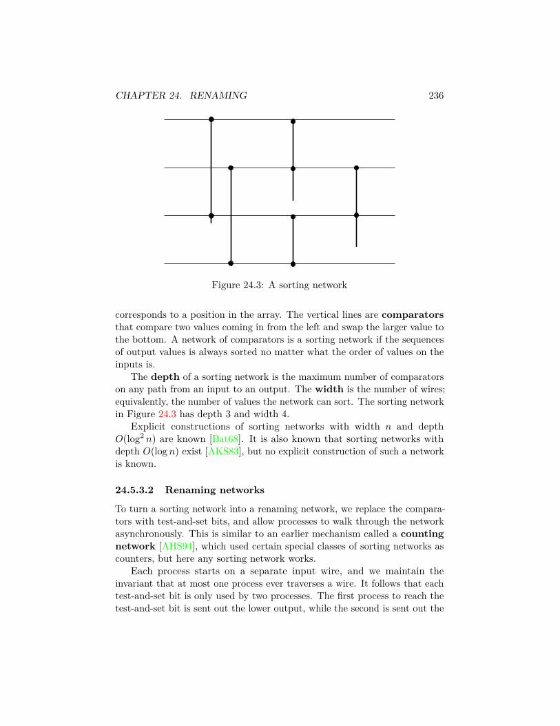
CHAPTER 24. RENAMING 236

Figure 24.3: A sorting network

corresponds to a position in the array. The vertical lines are comparatorsthat compare two values coming in from the left and swap the larger value tothe bottom. A network of comparators is a sorting network if the sequencesof output values is always sorted no matter what the order of values on theinputs is.

The depth of a sorting network is the maximum number of comparatorson any path from an input to an output. The width is the number of wires;equivalently, the number of values the network can sort. The sorting networkin Figure 24.3 has depth 3 and width 4.

Explicit constructions of sorting networks with width n and depthO(log2 n) are known [Bat68]. It is also known that sorting networks withdepth O(logn) exist [AKS83], but no explicit construction of such a networkis known.

24.5.3.2 Renaming networks

To turn a sorting network into a renaming network, we replace the compara-tors with test-and-set bits, and allow processes to walk through the networkasynchronously. This is similar to an earlier mechanism called a countingnetwork [AHS94], which used certain special classes of sorting networks ascounters, but here any sorting network works.

Each process starts on a separate input wire, and we maintain theinvariant that at most one process ever traverses a wire. It follows that eachtest-and-set bit is only used by two processes. The first process to reach thetest-and-set bit is sent out the lower output, while the second is sent out the

CHAPTER 24. RENAMING 237

upper output. If we imagine each process that participates in the protocolas a one and each process that doesn’t as a zero, the test-and-set bit actsas a comparator: if no processes show up on either input (two zeros), noprocesses leave (two zeros again); if processes show up on both inputs (twoones), processes leave on both (two ones again); and if only one process evershows up (a zero and a one), it leaves on the bottom output (zero and one,sorted). Because the original sorting network sorts all the ones to the bottomoutput wires, the corresponding renaming network sorts all the processesthat arrive to the bottom outputs. Label these outputs starting at 1 at thebottom to get renaming.

Since each test-and-set involves at most two processes, we can carry themout in O(1) expected register operations using, for example, the protocolof Tromp and Vitányi [TV02]. The expected cost for a process to acquirea name is then O(logn) (using an AKS [AKS83] sorting network). A morecomplicated construction in the Alistarh et al. paper shows how to makethis adaptive, giving an expected cost of O(log k) instead.

The problem with using an AKS network is that the AKS result isnon-constructive: what Ajtai, Komlós, and Szemerédi show is that thereis a particular randomized construction of candidate sorting networks thatsucceeds in producing a correct sorting network with nonzero (but very small)probability. Other disturbing features of this result are that we have noefficient way to test candidate sorting networks (determining if a network ofcomparators is in fact a sorting network is co-NP-hard), and the constantin the big-O for AKS is quite spectacularly huge. So it probably makesmore sense to think of renaming networks as giving renaming in O(log2 n)time, since this is the most efficient practical sorting network we currentlyknow about. This has led to efforts to produce O(log k)-work tight renamingalgorithms that don’t depend on AKS. So far this has not worked out in thestandard shared-memory model, even allowing test-and-sets.3

The use of test-and-sets to route processes to particular names is similar tothe line of test-and-sets proposed by Moir and Anderson [MA95] as describedin §24.4.5. Some differences between that protocol and renaming networksis that renaming networks do not by themselves give fetch-and-increment(although Alistarh et al. show how to build fetch-and-increment on top of

3The closest to this so far is an algorithm of Berenbrink et al. [BBE+15], who use anextended model that incorporates an extra primitive called a τ-register, which is basicallya collection of 2 logn test-and-set objects that are restricted so that at most τ < 2 logn ofthem can be set at a time. Adding this primitive to the model is not entirely cheating, asthe authors make a case that it could be plausibly implemented in hardware. But it doesmean that we don’t know what happens if we don’t have this additional primitive.

CHAPTER 24. RENAMING 238

renaming networks at a small additional cost), and renaming networks donot provide any mechanism for releasing names. The question of whether itis possible to get cheap long-lived strong renaming is still open.

24.5.4 Randomized loose renaming

Loose renaming should be easier than strong renaming, and using a random-ized algorithm it essentially reduces to randomized load balancing. A basicapproach is to use 2n names, and guard each with a test-and-set; becauseless than half of the names are taken at any given time, each process gets aname after O(1) tries and the most expensive renaming operation over all nprocesses takes O(logn) expected steps.

A more sophisticated version of this strategy, which appears in [AAGW13],uses n(1+ ε) output names to get O(log logn) maximum steps. The intuitionfor why this works is if n processes independently choose one of cn namesuniformly at random, then the expected number of collisions—pairs ofprocesses that choose the same name—is

(n2)/cn, or about n/2c. This may

seem like only a constant-factor improvement, but if we instead look at theratio between the survivors n/2c and the number of allocated names cn, wehave now moved from 1/c to 1/2c2. The 2 gives us some room to reduce thenumber of names in the next round, to cn/2, say, while still keeping a 1/c2

ratio of survivors to names.So the actual renaming algorithm consists of allocating cn/2i names to

round i, and squaring the ratio of survivors to names in each rounds. It onlytakes O(log logn) rounds to knock the ratio of survivors to names below1/n, so at this point it is likely that all processes will have finished. At thesame time, the sum over all rounds of the allocated names forms a geometricseries, so only O(n) names are needed altogether.

Swept under the carpet here is a lot of careful analysis of the probabilities.Unlike what happens with sifters (see §23.7), Jensen’s inequality goes thewrong way here, so some additional technical tricks are needed (see the paperfor details). But the result is that only O(log logn) rounds are to assignevery process a name with high probability, which is the best value currentlyknown.

There is a rather weak lower bound in the Alistarh et al. paper that showsthat Ω(log logn) steps are needed for some process in the worst case, underthe assumption that the renaming algorithm uses only test-and-set objectsand that a process acquires a name as soon as it wins some test-and-setobject. This does not give a lower bound on the problem in general, andindeed the renaming-network based algorithms discussed previously do not

CHAPTER 24. RENAMING 239

have this property. So the question of the exact complexity of randomizedloose renaming is still open.

Chapter 25

Software transactionalmemory

Last updated 2011. Some material may be out of date. If you are interestedin software transactional memory from a theoretical perspective, there is amore recent survey on this material by Attiya [Att14], available at http:// www. eatcs. org/ images/ bulletin/ beatcs112. pdf .

Software transactional memory, or STM for short, goes back toShavit and Touitou [ST97] based on earlier proposals for hardware supportfor transactions by Herlihy and Moss [HM93]. Recently very popular inprogramming language circles. We’ll give a high-level description of theShavit and Touitou results; for full details see the actual paper.

We start with the basic idea of a transaction. In a transaction, I read abunch of registers and update their values, and all of these operations appearto be atomic, in the sense that the transaction either happens completelyor not at all, and serializes with other transactions as if each occurredinstantaneously. Our goal is to implement this with minimal hardwaresupport, and use it for everything.

Generally we only consider static transactions where the set of memorylocations accessed is known in advance, as opposed to dynamic transac-tions where it may vary depending on what we read (for example, maybewe have to follow pointers through some data structure). Static transactionsare easier because we can treat them as multi-word read-modify-write.

Implementations are usually non-blocking: some infinite stream oftransactions succeed, but not necessarily yours. This excludes the simplestmethod based on acquiring locks, since we have to keep going even if a

240

CHAPTER 25. SOFTWARE TRANSACTIONAL MEMORY 241

lock-holder crashes, but is weaker than wait-freedom since we can havestarvation.

25.1 MotivationSome selling points for software transactional memory:

1. We get atomic operations without having to use our brains much.Unlike hand-coded atomic snapshots, counters, queues, etc., we have auniversal construction that converts any sequential data structure builton top of ordinary memory into a concurrent data structure. This isuseful since most programmers don’t have very big brains. We alsoavoid burdening the programmer with having to remember to lockthings.

2. We can build large shared data structures with the possibility ofconcurrent access. For example, we can implement atomic snapshots sothat concurrent updates don’t interfere with each other, or an atomicqueue where enqueues and dequeues can happen concurrently so longas the queue always has a few elements in it to separate the enqueuersand dequeuers.

3. We can execute atomic operations that span multiple data structures,even if the data structures weren’t originally designed to work together,provided they are all implemented using the STM mechanism. Thisis handy in classic database-like settings, as when we want to take $5from my bank account and put it in yours.

On the other hand, we now have to deal with the possibility that opera-tions may fail. There is a price to everything.

25.2 Basic approaches• Locking (not non-blocking). Acquire either a single lock for all of

memory (doesn’t allow much concurrency) or a separate lock for eachmemory location accessed. The second approach can lead to deadlockif we aren’t careful, but we can prove that if every transaction acquireslocks in the same order (e.g., by increasing memory address), thenwe never get stuck: we can order the processes by the highest lockacquired, and somebody comes out on top. Note that acquiring locks in

CHAPTER 25. SOFTWARE TRANSACTIONAL MEMORY 242

increasing order means that I have to know which locks I want beforeI acquire any of them, which may rule out dynamic transactions.

• Single-pointer compare-and-swap (called ”Herlihy’s method” in [ST97],because of its earlier use for constructing concurrent data structuresby Herlihy [Her93]). All access to the data structure goes througha pointer in a CAS. To execute a transaction, I make my own copyof the data structure, update it, and then attempt to redirect thepointer. Advantages: trivial to prove that the result is linearizable (thepointer swing is an atomic action) and non-blocking (somebody winsthe CAS); also, the method allows dynamic transactions (since you cando anything you want to your copy). Disadvantages: There’s a highoverhead of the many copies,1 and the single-pointer bottleneck limitsconcurrency even when two transactions use disjoint parts of memory.

• Multiword RMW: This is the approach suggested by Shavit and Touitou,which most subsequent work follows. As usually implemented, it onlyworks for static transactions. The idea is that I write down whatregisters I plan to update and what I plan to do to them. I thenattempt to acquire all the registers. If I succeed, I update all the values,store the old values, and go home. If I fail, it’s because somebody elsealready acquired one of the registers. Since I need to make sure thatsomebody makes progress (I may be the only process left alive), I’llhelp that other process finish its transaction if possible. Advantages:allows concurrency between disjoint transactions. Disadvantages: re-quires implementing multi-word RMW—in particular, requires thatany process be able to understand and simulate any other process’stransactions. Subsequent work often simplifies this to implementingmulti-word CAS, which is sufficient to do non-blocking multi-wordRMW since I can read all the registers I need (without any locking)and then do a CAS to update them (which fails only if somebody elsesucceeded).

25.3 Implementing multi-word RMWWe’ll give a sketchy description of Shavit and Touitou’s method [ST97],which essentially follows the locking approach but allows other processes tohelp dead ones so that locks are always released.

1This overhead can be reduced in many cases by sharing components, a subject thathas seen much work in the functional programming literature. See for example [Oka99].

CHAPTER 25. SOFTWARE TRANSACTIONAL MEMORY 243

The synchronization primitive used is LL/SC: LL (load-linked) readsa register and leaves our id attached to it, SC (store-conditional) writes aregister only if our id is still attached, and clears any other id’s that mightalso be attached. It’s easy to build a 1-register CAS (CAS1) out of this,though Shavit and Touitou exploit some additional power of LL/SC.

25.3.1 Overlapping LL/SC

The particular trick that gets used in the Shavit-Touitou protocol is touse two overlapping LL/SC pairs to do a CAS-like update on one memorylocation while checking that another memory location hasn’t changed. Thepurpose of this is to allow multiple processes to work on the same transaction(which requires the first CAS to avoid conflicts with other transactions) whilemaking sure that slow processes don’t cause trouble by trying to completetransactions that have already finished (the second check).

To see this in action, suppose we have a register r that we want to doa CAS on, while checking that a second register status is ⊥ (as opposed tosuccess or failure). If we execute the code fragment in Algorithm 25.1, it willsucceed only if nobody writes to status between its LL and SC and similarlyfor r; if this occurs, then at the time of LL(r), we know that status = ⊥, andwe can linearize the write to r at this time if we restrict all access to r to gothrough LL/SC.

1 if LL(status) = ⊥ then2 if LL(r) = oldValue then3 if SC(status,⊥) = true then4 SC(r, newValue)

Algorithm 25.1: Overlapping LL/SC

25.3.2 Representing a transaction

Transactions are represented by records rec. Each such record consists of astatus component that describes how far the transaction has gotten (neededto coordinate cooperating processes), a version component that distinguishesbetween versions that may reuse the same space (and that is used to shutdown the transaction when complete), a stable component that indicateswhen the initialization is complete, an Op component that describes theRMW to be performance, an array addresses[] of pointers to the arguments

CHAPTER 25. SOFTWARE TRANSACTIONAL MEMORY 244

to the RMW, and an array oldValues[] of old values at these addresses (forthe R part of the RMW). These are all initialized by the initiator of thetransaction, who will be the only process working on the transaction until itstarts acquiring locks.

25.3.3 Executing a transaction

Here we give an overview of a transaction execution:

1. Initialize the record rec for the transaction. (Only the initiator doesthis.)

2. Attempt to acquire ownership of registers in addresses[]. See theAcquireOwnerships code in the paper for details. The essential idea isthat we want to set the field owner[r] for each memory location r thatwe need to lock; this is done using an overlapping LL/SC as describedabove so that we only set owner[r] if (a) r is currently unowned, and(b) nothing has happened to rec.status or rec.version. Ownership isacquired in order of increasing memory address; if we fail to acquireownership for some r, our transaction fails. In case of failure, we setrec.status to failure and release all the locks we’ve acquired (checkingrec.version in the middle of each LL/SC so we don’t release locks fora later version using the same record). If we are the initiator of thistransaction, we will also go on to attempt to complete the transactionthat got in our way.

3. Do a LL on rec.status to see if AcquireOwnerships succeeded. If so,update the memory, store the old results in oldValues, and release theownerships. If it failed, release ownership and help the next transactionas described above.

Note that only an initiator helps; this avoids a long chain of helping andlimits the cost of each attempted transaction to the cost of doing two fulltransactions, while (as shown below) still allowing some transaction to finish.

25.3.4 Proof of linearizability

Intuition is:

• Linearizability follows from the linearizability of the locking protocol:acquiring ownership is equivalent to grabbing a lock, and updates occuronly when all registers are locked.

CHAPTER 25. SOFTWARE TRANSACTIONAL MEMORY 245

• Complications come from (a) two or more processes trying to completethe same transaction and (b) some process trying to complete an oldtransaction that has already terminated. For the first part we justmake sure that the processes don’t interfere with each other, e.g. I amhappy when trying to acquire a location if somebody else acquires it forthe same transaction. For the second part we have to check rec.statusand rec.version before doing just about anything. See the pseudocodein the paper for details on how this is done.

25.3.5 Proof of non-blockingness

To show that the protocol is non-blocking we must show that if an unboundednumber of transactions are attempted, one eventually succeeds. First observethat in order to fail, a transaction must be blocked by another transactionthat acquired ownership of a higher-address location than it did; eventuallywe run out of higher-address locations, so there is some transaction thatdoesn’t fail. Of course, this transaction may not succeed (e.g., if its initiatordies), but either (a) it blocks some other transaction, and that transaction’sinitiator will complete it or die trying, or (b) it blocks no future transactions.In the second case we can repeat the argument for the n − 1 survivingprocesses to show that some of them complete transactions, ignoring thestalled transaction from case (b).

25.4 ImprovementsOne downside of the Shavit and Touitou protocol is that it uses LL/SC veryaggressively (e.g., with overlapping LL/SC operations) and uses non-trivial(though bounded, if you ignore the ever-increasing version numbers) amountsof extra space. Subsequent work has aimed at knocking these down; forexample a paper by Harris, Fraser, and Pratt [HFP02] builds multi-registerCAS out of single-register CAS with O(1) extra bits per register. The proofof these later results can be quite involved; Harris et al., for example, basetheir algorithm on an implementation of 2-register CAS whose correctnesshas been verified only by machine (which may be a plus in some views).

25.5 LimitationsThere has been a lot of practical work on STM designed to reduce overheadon real hardware, but there’s still a fair bit of overhead. On the theory side,

CHAPTER 25. SOFTWARE TRANSACTIONAL MEMORY 246

a lower bound of Attiya, Hillel, and Milani [AHM09] shows that any STMsystem that guarantees non-interference between non-overlapping RMWtransactions has the undesirable property of making read-only transactionsas expensive as RMW transactions: this conflicts with the stated goalsof many practical STM implementations, where it is assumed that mosttransactions will be read-only (and hopefully cheap). So there is quite a bitof continuing research on finding the right trade-offs.

Chapter 26

Obstruction-freedom

Last updated 2011. Some material may be out of date. In particular: §26.3 hasnot been updated to include some more recent results [ACHS13, GHHW13];and §26.4 mostly follows the conference version [FHS05] of the Ellen-Hendler-Shavit paper and omits stronger results from the journal version [EHS12].

The gold standard for shared-memory objects is wait-freedom: I canfinish my operation in a bounded number of steps no matter what anybodyelse does. Like the gold standard in real life, this can be overly constraining.So researchers have developed several weaker progress guarantees that arenonetheless useful. The main ones are:

Lock-freedom An implementation is lock-free if infinitely many opera-tions finish in any infinite execution. In simpler terms, somebody alwaysmakes progress, but maybe not you. (Also called non-blocking.)

Obstruction-freedom An implementation is obstruction-free if, startingfrom any reachable configuration, any process can finish in a boundednumber of steps if all of the other processes stop. This definition wasproposed in 2003 by Herlihy, Luchangco, and Moir [HLM03]. In lowerbounds (e.g., the Jayanti-Tan-Toueg bound described in Chapter 20)essentially the same property is often called solo-terminating.

Both of these properties exclude traditional lock-based algorithms, wheresome process grabs a lock, updates the data structure, and then release thelock; if this process halts, no more operations finish. Both properties arealso weaker than wait-freedom. It is not hard to show that lock-freedom is a

247

CHAPTER 26. OBSTRUCTION-FREEDOM 248

stronger condition that obstruction-freedom: given a lock-free implementa-tion, if we can keep some single process running forever in isolation, we getan infinite execution with only finitely many completed operations. So wehave a hierarchy: wait-free > lock-free > obstruction-free > locking.

26.1 Why build obstruction-free algorithms?The pitch is similar to the pitch for building locking algorithms: an obstruction-free algorithm might be simpler to design, implement, and reason aboutthan a more sophisticated algorithm with stronger properties. Unlike lockingalgorithms, an obstruction-free algorithm won’t fail because some processdies holding the lock; instead, it fails if more than one process runs thealgorithm at the same time. This possibility may be something we canavoid by building a contention manager, a high-level protocol that detectscontention and delays some processes to avoid it (say, using randomizedexponential back-off).

26.2 Examples

26.2.1 Lock-free implementations

Pretty much anything built using compare-and-swap or LL/SC ends upbeing lock-free. A simple example would be a counter, where an incrementoperation does

1 x← LL(C)2 SC(C, x+ 1)

This is lock-free (the only way to prevent a store-conditional from suc-ceeding is if some other store-conditional succeeds, giving infinitely manysuccessful increments) but not wait-free (I can starve). It’s also obstruction-free, but since it’s already lock-free we don’t care about that.

26.2.2 Double-collect snapshots

Similarly, suppose we are doing atomic snapshots. We know that thereexist wait-free implementations of atomic snapshots, but they are subtle andconfusing. So we want to do something simpler, and hope that we at leastget obstruction-freedom.

CHAPTER 26. OBSTRUCTION-FREEDOM 249

If we do double-collects, that is, we have updates just write to a registerand have snapshots repeatedly collect until they get two collects in a rowwith the same values, then any snapshot that finishes is correct (assuming noupdaters ever write the same value twice, which we can enforce with nonces).This isn’t wait-free, because we can keep a snapshot going forever by doinga lot of updates. It is lock-free, because we have to keep doing updates tomake this happen.

We can make this merely obstruction-free if we work hard (there is no rea-son to do this, but it illustrates the difference between lock-freedom—good—andobstruction-freedom—not so good). Suppose that every process keeps a countof how many collects it has done in a register that is included in other pro-cess’s collects (but not its own). Then two concurrent scans can stall eachother forever (the implementation is not lock-free), but if only one is runningit completes two collects in O(n) operations without seeing any changes (itis obstruction-free).

26.2.3 Software transactional memory

Similar things happen with software transactional memory (see Chapter 25).Suppose that I have an implementation of multiword compare-and-swap, andI want to carry out a transaction. I read all the values I need, then executean MCAS operation that only updates if these values have not changed. Theresulting algorithm is lock-free (if my transaction fails, it’s because someupdate succeeded). If however I am not very clever and allow some values toget written outside of transactions, then I might only be obstruction-free.

26.2.4 Obstruction-free test-and-set

Algorithm 26.1 gives an implementation of 2-process test-and-set from atomicregisters that is obstruction-free; this demonstrates that obstruction-freedomlets us evade the wait-free impossibility results implied by the consensushierarchy ([Her91b], discussed in Chapter 18).

The basic idea goes back to the racing counters technique used inconsensus protocols starting with Chor, Israeli, and Li [CIL94], and there issome similarity to a classic randomized wait-free test-and-set due to Trompand Vitányi [TV02]. Each process keeps a position x in memory that it alsostores from time to time in its register a[i]. If a process gets 2 steps aheadof the other process (as observed by comparing x to a[i − 1], it wins thetest-and-set; if a process falls one or more steps behind, it (eventually) loses.To keep space down and guarantee termination in bounded time, all values

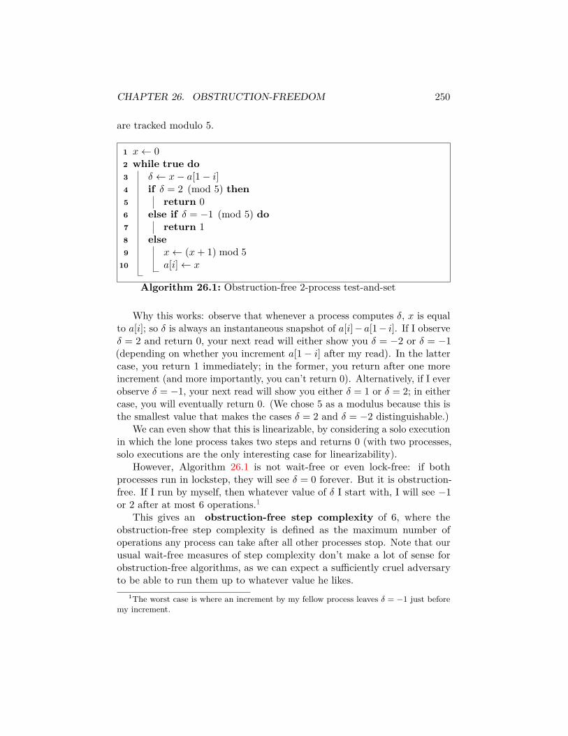
CHAPTER 26. OBSTRUCTION-FREEDOM 250

are tracked modulo 5.

1 x← 02 while true do3 δ ← x− a[1− i]4 if δ = 2 (mod 5) then5 return 06 else if δ = −1 (mod 5) do7 return 18 else9 x← (x+ 1) mod 5

10 a[i]← x

Algorithm 26.1: Obstruction-free 2-process test-and-set

Why this works: observe that whenever a process computes δ, x is equalto a[i]; so δ is always an instantaneous snapshot of a[i]−a[1− i]. If I observeδ = 2 and return 0, your next read will either show you δ = −2 or δ = −1(depending on whether you increment a[1− i] after my read). In the lattercase, you return 1 immediately; in the former, you return after one moreincrement (and more importantly, you can’t return 0). Alternatively, if I everobserve δ = −1, your next read will show you either δ = 1 or δ = 2; in eithercase, you will eventually return 0. (We chose 5 as a modulus because this isthe smallest value that makes the cases δ = 2 and δ = −2 distinguishable.)

We can even show that this is linearizable, by considering a solo executionin which the lone process takes two steps and returns 0 (with two processes,solo executions are the only interesting case for linearizability).

However, Algorithm 26.1 is not wait-free or even lock-free: if bothprocesses run in lockstep, they will see δ = 0 forever. But it is obstruction-free. If I run by myself, then whatever value of δ I start with, I will see −1or 2 after at most 6 operations.1

This gives an obstruction-free step complexity of 6, where theobstruction-free step complexity is defined as the maximum number ofoperations any process can take after all other processes stop. Note that ourusual wait-free measures of step complexity don’t make a lot of sense forobstruction-free algorithms, as we can expect a sufficiently cruel adversaryto be able to run them up to whatever value he likes.

1The worst case is where an increment by my fellow process leaves δ = −1 just beforemy increment.

CHAPTER 26. OBSTRUCTION-FREEDOM 251

Building a tree of these objects as in §22.2 gives n-process test-and-setwith obstruction-free step complexity O(logn).

26.2.5 An obstruction-free deque

(We probably aren’t going to do this in class.)So far we don’t have any good examples of why we would want to be

obstruction-free if our algorithm is based on CAS. So let’s describe the caseHerlihy et al. suggested.

A deque is a generalized queue that supports push and pop at both ends(thus it can be used as either a queue or a stack, or both). A classic problemin shared-memory objects is to build a deque where operations at one end ofthe deque don’t interfere with operations at the other end. While there existlock-free implementation with this property, there is a particularly simpleimplementation using CAS that is only obstruction-free.

Here’s the idea: we represent the deque as an infinitely-long array ofcompare-and-swap registers (this is a simplification from the paper, whichgives a bounded implementation of a bounded deque). The middle of thedeque holds the actual contents. To the right of this region is an infinitesequence of right null (RN) values, which are assumed never to appearas a pushed value. To the left is a similar infinite sequence of left null(LN) values. Some magical external mechanism (called an oracle in thepaper) allows processes to quickly find the first null value at either end ofthe non-null region; the correctness of the protocol does not depend on theproperties of the oracle, except that it has to point to the right place at leastsome of the time in a solo execution. We also assume that each cell holds aversion number whose only purpose is to detect when somebody has fiddledwith the cell while we aren’t looking (if we use LL/SC, we can drop this).

Code for rightPush and rightPop is given in Algorithm 26.2 (the codefor leftPush and leftPop is symmetric).

It’s easy to see that in a solo execution, if the oracle doesn’t lie, eitheroperation finishes and returns a plausible value after O(1) operations. Sothe implementation is obstruction-free. But is it also correct?

To show that it is, we need to show that any execution leaves the dequein a sane state, in particular that it preserves the invariant that the dequeconsists of left-nulls followed by zero or more values followed by right-nulls,and that the sequence of values in the queue is what it should be.

This requires a detailed case analysis of which operations interfere witheach other, which can be found in the original paper. But we can give someintuition here. The two CAS operations in rightPush or rightPop succeed

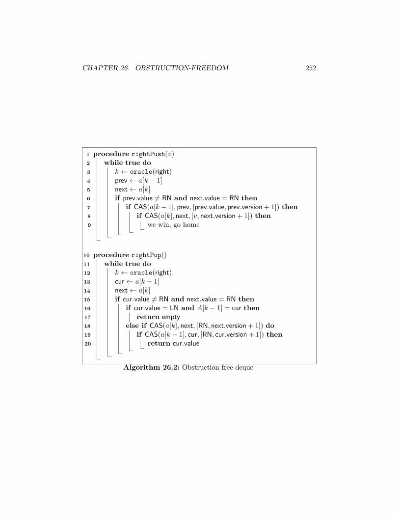
CHAPTER 26. OBSTRUCTION-FREEDOM 252

1 procedure rightPush(v)2 while true do3 k ← oracle(right)4 prev← a[k − 1]5 next← a[k]6 if prev.value 6= RN and next.value = RN then7 if CAS(a[k − 1], prev, [prev.value, prev.version + 1]) then8 if CAS(a[k], next, [v, next.version + 1]) then9 we win, go home

10 procedure rightPop()11 while true do12 k ← oracle(right)13 cur← a[k − 1]14 next← a[k]15 if cur.value 6= RN and next.value = RN then16 if cur.value = LN and A[k − 1] = cur then17 return empty18 else if CAS(a[k], next, [RN, next.version + 1]) do19 if CAS(a[k − 1], cur, [RN, cur.version + 1]) then20 return cur.value

Algorithm 26.2: Obstruction-free deque

CHAPTER 26. OBSTRUCTION-FREEDOM 253

only if neither register was modified between the preceding read and theCAS. If both registers are unmodified at the time of the second CAS, thenthe two CAS operations act like a single two-word CAS, which replaces theprevious values (top,RN) with (top, value) in rightPush or (top, value) with(top,RN) in rightPop; in either case the operation preserves the invariant.So the only way we get into trouble is if, for example, a rightPush does aCAS on a[k−1] (verifying that it is unmodified and incrementing the versionnumber), but then some other operation changes a[k − 1] before the CAS ona[k]. If this other operation is also a rightPush, we are happy, because itmust have the same value for k (otherwise it would have failed when it sawa non-null in a[k − 1]), and only one of the two right-pushes will succeedin applying the CAS to a[k]. If the other operation is a rightPop, then itcan only change a[k − 1] after updating a[k]; but in this case the update toa[k] prevents the original right-push from changing a[k]. With some moretedious effort we can similarly show that any interference from leftPush orleftPop either causes the interfering operation or the original operation tofail. This covers 4 of the 16 cases we need to consider. The remaining caseswill be brushed under the carpet to avoid further suffering.

26.3 Boosting obstruction-freedom to wait-freedomNaturally, having an obstruction-free implementation of some object isnot very helpful if we can’t guarantee that some process eventually getsits unobstructed solo execution. In general, we can’t expect to be ableto do this without additional assumptions; for example, if we could, wecould solve consensus using a long sequence of adopt-commit objects withno randomization at all.2 So we need to make some sort of assumptionabout timing, or find somebody else who has already figured out the rightassumption to make.

Those somebodies turn out to be Faith Ellen Fich, Victor Luchangco,Mark Moir, and Nir Shavit, who give an algorithm for boosting obstruction-freedom to wait-freedom [FLMS05]. The timing assumption is unknown-bound semisynchrony, which means that in any execution there is somemaximum ratio R between the shortest and longest time interval betweenany two consecutive steps of the same non-faulty process, but the processes

2This fact was observed by Herlihy et al. [HLM03] in their original obstruction-freepaper; it also implies that there exists a universal obstruction-free implementation ofanything based on Herlihy’s universal construction.

CHAPTER 26. OBSTRUCTION-FREEDOM 254

don’t know what this ratio is.3 In particular, if I can execute more than Rsteps without you doing anything, I can reasonably conclude that you aredead—the semisynchrony assumption thus acts as a failure detector.

The fact that R is unknown might seem to be an impediment to usingthis failure detector, but we can get around this. The idea is to start witha small guess for R; if a process is suspected but then wakes up again, weincrement the guess. Eventually, the guessed value is larger than the correctvalue, so no live process will be falsely suspected after this point. Formally,this gives an eventually perfect (♦P ) failure detector, although the algorithmdoes not specifically use the failure detector abstraction.

To arrange for a solo execution, when a process detects a conflict (becauseits operation didn’t finish quickly), it enters into a “panic mode” where pro-cesses take turns trying to finish unmolested. A fetch-and-increment registeris used as a timestamp generator, and only the process with the smallesttimestamp gets to proceed. However, if this process is too sluggish, otherprocesses may give up and overwrite its low timestamp with ∞, temporarilyending its turn. If the sluggish process is in fact alive, it can restore its lowtimestamp and kill everybody else, allowing it to make progress until someother process declares it dead again.

The simulation works because eventually the mechanism for detectingdead processes stops suspecting live ones (using the technique describedabove), so the live process with the winning timestamp finishes its operationwithout interference. This allows the next process to proceed, and eventuallyall live processes complete any operation they start, giving the wait-freeproperty.

The actual code is in Algorithm 26.3. It’s a rather long algorithm butmost of the details are just bookkeeping.

The preamble before entering PANIC mode is a fast-path computationthat allows a process that actually is running in isolation to skip testingany timestamps or doing any extra work (except for the one register read ofPANIC). The assumption is that the constant B is set high enough that anyprocess generally will finish its operation in B steps without interference. Ifthere is interference, then the timestamp-based mechanism kicks in: we graba timestamp out of the convenient fetch-and-add register and start sluggingit out with the other processes.

(A side note: while the algorithm as presented in the paper assumesa fetch-and-add register, any timestamp generator that delivers increasing

3This is a much older model, which goes back to a famous paper of Dwork, Lynch, andStockmeyer [DLS88].

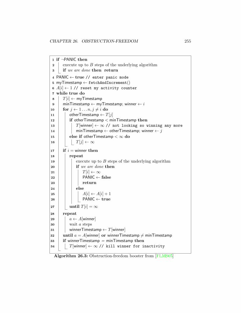
CHAPTER 26. OBSTRUCTION-FREEDOM 255

1 if ¬PANIC then2 execute up to B steps of the underlying algorithm3 if we are done then return4 PANIC← true // enter panic mode5 myTimestamp← fetchAndIncrement()6 A[i]← 1 // reset my activity counter7 while true do8 T [i]← myTimestamp9 minTimestamp← myTimestamp; winner← i

10 for j ← 1 . . . n, j 6= i do11 otherTimestamp← T [j]12 if otherTimestamp < minTimestamp then13 T [winner]←∞ // not looking so winning any more14 minTimestamp← otherTimestamp; winner← j

15 else if otherTimestamp <∞ do16 T [j]←∞

17 if i = winner then18 repeat19 execute up to B steps of the underlying algorithm20 if we are done then21 T [i]←∞22 PANIC← false23 return24 else25 A[i]← A[i] + 126 PANIC← true27 until T [i] =∞28 repeat29 a← A[winner]30 wait a steps31 winnerTimestamp← T [winner]32 until a = A[winner] or winnerTimestamp 6= minTimestamp33 if winnerTimestamp = minTimestamp then34 T [winner]←∞ // kill winner for inactivity

Algorithm 26.3: Obstruction-freedom booster from [FLMS05]

CHAPTER 26. OBSTRUCTION-FREEDOM 256

values over time will work. So if we want to limit ourselves to atomic registers,we could generate timestamps by taking snapshots of previous timestamps,adding 1, and appending process ids for tie-breaking.)

Once I have a timestamp, I try to knock all the higher-timestamp processesout of the way (by writing ∞ to their timestamp registers). If I see a smallertimestamp than my own, I’ll drop out myself (T [i]←∞), and fight on behalfof its owner instead. At the end of the j loop, either I’ve decided I am thewinner, in which case I try to finish my operation (periodically checking T [i]to see if I’ve been booted), or I’ve decided somebody else is the winner, inwhich case I watch them closely and try to shut them down if they are tooslow (T [winner] ← ∞). I detect slow processes by inactivity in A[winner];similarly, I signal my own activity by incrementing A[i]. The value in A[i]is also used as an increasing guess for the time between increments of A[i];eventually this exceeds the R(B +O(1)) operations that I execute betweenincrementing it.

We still need to prove that this all works. The essential idea is to showthat whatever process has the lowest timestamp finishes in a bounded numberof steps. To do so, we need to show that other processes won’t be fighting itin the underlying algorithm. Call a process active if it is in the loop guardedby the “if i = winner” statement. Lemma 1 from the paper states:

Lemma 26.3.1 ([FLMS05, Lemma 1]). If processes i and j are both active,then T [i] =∞ or T [j] =∞.

Proof. Assume without loss of generality that i last set T [i] to myTimestampin the main loop after j last set T [j]. In order to reach the active loop, imust read T [j]. Either T [j] =∞ at this time (and we are done, since only jcan set T [j] <∞), or T [j] is greater than i’s timestamp (or else i wouldn’tthink it’s the winner). In the second case, i sets T [j] =∞ before enteringthe active loop, and again the claim holds.

The next step is to show that if there is some process i with a minimumtimestamp that executes infinitely many operations, it increments A[i] in-finitely often (thus eventually making the failure detector stop suspecting it).This gives us Lemma 2 from the paper:

Lemma 26.3.2 ([FLMS05, Lemma 2]). Consider the set of all processes thatexecute infinitely many operations without completing an operation. Supposethis set is non-empty, and let i hold the minimum timestamp of all theseprocesses. Then i is not active infinitely often.

CHAPTER 26. OBSTRUCTION-FREEDOM 257

Proof. Suppose that from some time on, i is active forever, i.e., it neverleaves the active loop. Then T [i] < ∞ throughout this interval (or else ileaves the loop), so for any active j, T [j] =∞ by the preceding lemma. Itfollows that any active T [j] leaves the active loop after B +O(1) steps of j(and thus at most R(B +O(1)) steps of i). Can j re-enter? If j’s timestampis less than i’s, then j will set T [i] =∞, contradicting our assumption. Butif j’s timestamp is greater than i’s, j will not decide it’s the winner andwill not re-enter the active loop. So now we have i alone in the active loop.It may still be fighting with processes in the initial fast path, but since isets PANIC every time it goes through the loop, and no other process resetsPANIC (since no other process is active), no process enters the fast path aftersome bounded number of i’s steps, and every process in the fast path leavesafter at most R(B +O(1)) of i’s steps. So eventually i is in the loop aloneforever—and obstruction-freedom means that it finishes its operation andleaves. This contradicts our initial assumption that i is active forever.

So now we want to argue that our previous assumption that there existsa bad process that runs forever without winning leads to a contradiction, byshowing that the particular i from Lemma 26.3.2 actually finishes (note thatLemma 26.3.2 doesn’t quite do this—we only show that i finishes if it staysactive long enough, but maybe it doesn’t stay active).

Suppose i is as in Lemma 26.3.2. Then i leaves the active loop infinitelyoften. So in particular it increments A[i] infinitely often. After some finitenumber of steps, A[i] exceeds the limit R(B+O(1)) on how many steps someother process can take between increments of A[i]. For each other process j,either j has a lower timestamp than i, and thus finishes in a finite number ofsteps (from the premise of the choice of i), or j has a higher timestamp thani. Once we have cleared out all the lower-timestamp processes, we follow thesame logic as in the proof of Lemma 26.3.2 to show that eventually (a) i setsT [i] < ∞ and PANIC = true, (b) each remaining j observes T [i] < ∞ andPANIC = true and reaches the waiting loop, (c) all such j wait long enough(since A[i] is now very big) that i can finish its operation. This contradictsthe assumption that i never finishes the operation and completes the proof.

26.3.1 Cost

If the parameters are badly tuned, the potential cost of this construction isquite bad. For example, the slow increment process for A[i] means that thetime a process spends in the active loop even after it has defeated all otherprocesses can be as much as the square of the time it would normally take

CHAPTER 26. OBSTRUCTION-FREEDOM 258

to complete an operation alone—and every other process may pay R timesthis cost waiting. This can be mitigated to some extent by setting B highenough that a winning process is likely to finish in its first unmolested passthrough the loop (recall that it doesn’t detect that the other processes havereset T [i] until after it makes its attempt to finish). An alternative mightbe to double A[i] instead of incrementing it at each pass through the loop.However, it is worth noting (as the authors do in the paper) that nothingprevents the underlying algorithm from incorporating its own contentionmanagement scheme to ensure that most operations complete in B stepsand PANIC mode is rarely entered. So we can think of the real function ofthe construction as serving as a backstop to some more efficient heuristicapproach that doesn’t necessarily guarantee wait-free behavior in the worstcase.

26.4 Lower bounds for lock-free protocolsSo far we have seen that obstruction-freedom buys us an escape from theimpossibility results that plague wait-free constructions, while still allowingpractical implementations of useful objects under plausible timing assump-tions. Yet all is not perfect: it is still possible to show non-trivial lowerbounds on the costs of these implementations in the right model. We willpresent one of these lower bounds, the linear-contention lower bound of Ellen,Hendler, and Shavit [EHS12].4 First we have to define what is meant bycontention.

26.4.1 Contention

A limitation of real shared-memory systems is that physics generally won’tpermit more than one process to do something useful to a shared objectat a time. This limitation is often ignored in computing the complexity ofa shared-memory distributed algorithm (and one can make arguments forignoring it in systems where communication costs dominate update costs inthe shared-memory implementation), but it is useful to recognize it if wecan’t prove lower bounds otherwise. Complexity measures that take the costof simultaneous access into account go by the name of contention.

The particular notion of contention used in the Ellen et al. paper is anadaptation of the contention measure of Dwork, Herlihy, andWaarts [DHW97].

4The result first appeared in FOCS in 2005 [FHS05], with a small but easily fixed bug inthe definition of the class of objects the proof applies to. We’ll use the corrected definitionfrom the journal version.

CHAPTER 26. OBSTRUCTION-FREEDOM 259

The idea is that if I access some shared object, I pay a price in memorystalls for all the other processes that are trying to access it at the same timebut got in first. In the original definition, given an execution of the formAφ1φ2 . . . φkφA

′, where all operations φi are applied to the same object as φ,and the last operation in A is not, then φk incurs k memory stalls. Ellen etal. modify this to only count sequences of non-trivial operations, where anoperation is non-trivial if it changes the state of the object in some states(e.g., writes, increments, compare-and-swap—but not reads). Note that thischange only strengthens the bound they eventually prove, which shows thatin the worst case, obstruction-free implementations of operations on objectsin a certain class incur a linear number of memory stalls (possibly spreadacross multiple base objects).

26.4.2 The class G

The Ellen et al. bound is designed to be as general as possible, so theauthors define a class G of objects to which it applies. As is often the casein mathematics, the underlying meaning of G is “a reasonably large classof objects for which this particular proof works,” but the formal definitionis given in terms of when certain operations of the implemented object areaffected by the presence or absence of other operations—or in other words,when those other operations need to act on some base object in order to letlater operations know they occurred.

An object is in class G if it has some operation Op and initial state ssuch that for any two processes p and q and every sequence of operationsAφA′, where

1. φ is an instance of Op executed by p,

2. no operation in A or A′ is executed by p,

3. no operation in A′ is executed by q, and

4. no two operations in A′ are executed by the same process;

then there exists a sequence of operations Q by q such that for every sequenceHφH ′ where

1. HH ′ is an interleaving of Q and the sequences AA′|r for each processr,

2. H ′ contains no operations of q, and

CHAPTER 26. OBSTRUCTION-FREEDOM 260

3. no two operations in H ′ are executed by the same process;

then the return value of φ to p changes depending on whether it occurs afterAφ or Hφ.

This is where “makes the proof work” starts looking like a much simplerdefinition. The intuition is that deep in the guts of the proof, we are going tobe injecting some operations of q into an existing execution (hence adding Q),and we want to do it in a way that forces q to operate on some object that pis looking at (hence the need for Aφ to return a different value from Hφ),without breaking anything else that is going on (all the rest of the conditions).The reason for pulling all of these conditions out of the proof into a separatedefinition is that we also want to be able to show that particular classes ofreal objects satisfy the conditions required by the proof, without having toput a lot of special cases into the proof itself.

Lemma 26.4.1. A mod-m fetch-and-increment object, with m ≥ n, is in G.

Proof. This is a classic proof-by-unpacking-the-definition. Pick some ex-ecution AφA′ satisfying all the conditions, and let a be the number offetch-and-increments in A and a′ the number in A′. Note a′ ≤ n− 2, sinceall operations in A′ are by different processes.

Now let Q be a sequence of n− a′ − 1 fetch-and-increments by q, and letHH ′ be an interleaving of Q and the sequences AA′|r for each r, where H ′includes no two operation of the same process and no operations at all ofq. Let h, h′ be the number of fetch-and-increments in H, H ′, respectively.Then h + h′ = a + a′ + (n − a′ − 1) = n + a − 1 and h′ ≤ n − 2 (since H ′contains at most one fetch-and-increment for each process other than p andq). This gives h ≥ (n+ a+ 1)− (n− 2) = a+ 1 and h ≤ n+ a− 1, and thereturn value of φ after Hφ is somewhere in this range mod m. But none ofthese values is equal to a mod m (that’s why we specified m ≥ n, althoughas it turns out m ≥ n − 1 would have been enough), so we get a differentreturn value from Hφ than from Aφ.

As a corollary, we also get stock fetch-and-increment registers, since wecan build mod-m registers from them by taking the results mod m.

A second class of class-G objects is obtained from snapshot:

Lemma 26.4.2. Single-writer snapshot objects are in G.55For the purposes of this lemma, “single-writer” means that each segment can be

written to by only one process, not that there is only one process that can execute updateoperations.

CHAPTER 26. OBSTRUCTION-FREEDOM 261

Proof. Let AφA′ be as in the definition, where φ is a scan operation. Let Qconsist of a single update operation by q that changes its segment. Thenin the interleaved sequence HH ′, this update doesn’t appear in H ′ (it’sforbidden), so it must be in H. Nobody can overwrite the result of theupdate (single-writer!), so it follows that Hφ returns a different snapshotfrom Aφ.

26.4.3 The lower bound proof

Theorem 26.4.3 ([EHS12, Theorem 5.2]). For any obstruction-free imple-mentation of some object in class G from RMW base objects, there is anexecution in which some operation incurs n− 1 stalls.

We can’t do better than n − 1, because it is easy to come up withimplementations of counters (for example) that incur at most n− 1 stalls.Curiously, we can even spread the stalls out in a fairly arbitrary way overmultiple objects, while still incurring at most n− 1 stalls. For example, acounter implemented using a single counter (which is a RMW object) getsexactly n− 1 stalls if n− 1 processes try to increment it at the same time,delaying the remaining process. At the other extreme, a counter implementedby doing a collect over n− 1 single-writer registers (also RMW objects) getsat least n− 1 stalls—distributed as one per register—if each register has awrite delivered to it while the reader waiting to read it during its collect. Sowe have to allow for the possibility that stalls are concentrated or scatteredor something in between, as long as the total number adds up at least n− 1.

The proof supposes that the theorem is not true and then shows how toboost an execution with a maximum number k < n− 1 stalls to an executionwith k + 1 stalls, giving a contradiction. (Alternatively, we can read theproof as giving a mechanism for generating an (n − 1)-stall execution byrepeated boosting, starting from the empty execution.)

This is pretty much the usual trick: we assume that there is a class ofbad executions, then look for an extreme member of this class, and show thatit isn’t as extreme as we thought. In doing so, we can restrict our attentionto particularly convenient bad executions, so long as the existence of somebad execution implies the existence of a convenient bad execution.

Formally, the authors define a k-stall execution for process p as anexecution Eσ1 . . . σi where E and σi are sequence of operations such that:

1. p does nothing in E,

2. Sets of processes Sj , j = 1 . . . i, whose union S =⋃ij=1 Sj has size k, are

each covering objects Oj after E with pending non-trivial operations,

CHAPTER 26. OBSTRUCTION-FREEDOM 262

3. Each σj consists of p applying events by itself until it is about to applyan event to Oj , after which each process in Sj accesses Oj , after whichp accesses Oj .

4. All processes not in S are idle after E,

5. p starts at most one operation of the implemented object in σ1 . . . σi,and

6. In every extension of E in which p and the processes in S don’t takesteps, no process applies a non-trivial event to any base object accessedin σ1 . . . σi. (We will call this the weird condition below.)

So this definition includes both the fact that p incurs k stalls and someother technical details that make the proof go through. The fact that pincurs k stalls follows from observing that it incurs |Sj | stalls in each segmentσj , since all processes in Sj access Oj just before p does.

Note that the empty execution is a 0-stall execution (with i = 0) by thedefinition. This shows that a k-stall execution exists for some k.

Note also that the weird condition is pretty strong: it claims not onlythat there are no non-trivial operation on O1 . . .Oi in τ , but also that thereare no non-trivial operations on any objects accessed in σ1 . . . σi, which mayinclude many more objects accessed by p.6

We’ll now show that if a k-stall execution exists, for k ≤ n− 2, then a(k+k′)-stall execution exists for some k′ > 0. Iterating this process eventuallyproduces an (n− 1)-stall execution.

Start with some k-stall execution Eσ1 . . . σi. Extend this execution bya sequence of operations σ in which p runs in isolation until it finishes itsoperation φ (which it may start in σ if it hasn’t done so already), then eachprocess in S runs in isolation until it completes its operation. Now linearizethe high-level operations completed in Eσ1 . . . σiσ and factor them as AφA′as in the definition of class G.

Let q be some process not equal to p or contained in any Sj (this is wherewe use the assumption k ≤ n− 2). Then there is some sequence of high-leveloperations Q of q such that Hφ does not return the same value as Aφ forany interleaving HH ′ of Q with the sequences of operations in AA′ satisfyingthe conditions in the definition. We want to use this fact to shove at leastone more memory stall into Eσ1 . . . σiσ, without breaking any of the otherconditions that would make the resulting execution a (k+ k′)-stall execution.

6And here is where I screwed up in class on 2011-11-14, by writing the condition as theweaker requirement that nobody touches O1 . . .Oi.

CHAPTER 26. OBSTRUCTION-FREEDOM 263

Consider the extension τ of E where q runs alone until it finishes everyoperation in Q. Then τ applies no nontrivial events to any base objectaccessed in σ1 . . . σk, (from the weird condition on k-stall executions) andthe value of each of these base objects is the same after E and Eτ , and thusis also the same after Eσ1 . . . σk and Eτσ1 . . . σk.

Now let σ′ be the extension of Eτσ1 . . . σk defined analogously to σ:p finishes, then each process in each Sj finishes. Let HφH ′ factor thelinearization of Eτσ1 . . . σiσ

′. Observe that HH ′ is an interleaving of Q andthe high-level operations in AA′, that H ′ contains no operations by q (theyall finished in τ , before φ started), and that H ′ contains no two operations bythe same process (no new high-level operations start after φ finishes, so thereis at most one pending operation per process in S that can be linearizedafter φ).

Now observe that q does some non-trivial operation in τ to some baseobject accessed by p in σ. If not, then p sees the same responses in σ′ and inσ, and returns the same value, contradicting the definition of class G.

So does q’s operation in τ cause a stall in σ? Not necessarily: theremay be other operations in between. Instead, we’ll use the existence of q’soperation to demonstrate the existence of at least one operation, possibly bysome other process we haven’t even encountered yet, that does cause a stall.We do this by considering the set F of all finite extensions of E that are freeof p and S operations, and look for an operation that stalls p somewhere inthis infinitely large haystack.

Let Oi+1 be the first base object accessed by p in σ that is also accessedby some non-trivial event in some sequence in F . We will show two things:first, that Oi+1 exists, and second, that Oi+1 is distinct from the objectsO1 . . .Oi. The first part follows from the fact that τ is in F , and we havejust shown that τ contains a non-trivial operation (by q) on a base objectaccessed by p in σ. For the second part, we use the weird condition on k-stallexecutions again: since every extension of E in F is (p∪S)-free, no processapplies a non-trivial event to any base object accessed in σ1 . . . σi, whichincludes all the objects O1 . . .Oi.

You’ve probably guessed that we are going to put our stalls in on Oi+1.We choose some extension X from F that maximizes the number of processeswith simultaneous pending non-trivial operations on Oi+1 (we’ll call this setof processes Si+1 and let |Si+1| be the number k′ > 0 we’ve been waiting for),and let E′ be the minimum prefix of X such that these pending operationsare still pending after EE′.

We now look at the properties of EE′. We have:

CHAPTER 26. OBSTRUCTION-FREEDOM 264

• EE′ is p-free (follows from E being p-free and E′ ∈ F , since everythingin F is p-free).

• Each process in Sj has a pending operation on Oj after EE′ (it didafter E, and didn’t do anything in E′).

This means that we can construct an execution EE′σ1 . . . σiσi+1 thatincludes k + k′ memory stalls, by sending in the same sequences σ1 . . . σi asbefore, then appending a new sequence of events where (a) p does all of itsoperations in σ up to its first operation on Oi+1; then (b) all the processes inthe set Si+1 of processes with pending events on Oi+1 execute their pendingevents on Oi+1; then (c) p does its first access to Oi+1 from σ. Note that inaddition to giving us k + k′ memory stalls, σi+1 also has the right structurefor a (k + k′)-stall execution. But there is one thing missing: we have toshow that the weird condition on further extensions still holds.

Specifically, letting S′ = S∪Si+1, we need to show that any (p∪S′)-freeextension α of EE′ includes a non-trivial access to a base object accessedin σ1 . . . σi+1. Observe first that since α is (p ∪ S′)-free, then E′α is(p ∪ S)-free, and so it’s in F : so by the weird condition on Eσ1 . . . σi, E′αdoesn’t have any non-trivial accesses to any object with a non-trivial accessin σ1 . . . σi. So we only need to squint very closely at σi+1 to make sure itdoesn’t get any objects in there either.

Recall that σi+1 consists of (a) a sequence of accesses by p to objectsalready accessed in σ1 . . . σi (already excluded); (b) an access of p to Oi+1;and (c) a bunch of accesses by processes in Si+1 to Oi+1. So we only needto show that α includes no non-trivial accesses to Oi+1. Suppose that itdoes: then there is some process that eventually has a pending non-trivialoperation on Oi+1 somewhere in α. If we stop after this initial prefix α′ of α,we get k′ + 1 processes with pending operations on Oi+1 in EE′α′. But thenE′α′ is an extension of E with k′ + 1 processes with a simultaneous pendingoperation on Oi+1. This contradicts the choice of X to maximize k′. So ifour previous choice was in fact maximal, the weird condition still holds, andwe have just constructed a (k + k′)-stall execution. This concludes the proof.

26.4.4 Consequences

We’ve just shown that counters and snapshots have (n− 1)-stall executions,because they are in the class G. A further, rather messy argument (given inthe Ellen et al. paper) extends the result to stacks and queues, obtaining aslightly weaker bound of n total stalls and operations for some process in

CHAPTER 26. OBSTRUCTION-FREEDOM 265

the worst case.7 In both cases, we can’t expect to get a sublinear worst-casebound on time under the reasonable assumption that both a memory stalland an actual operation takes at least one time unit. This puts an inherentbound on how well we can handle hot spots for many practical objects, andmeans that in an asynchronous system, we can’t solve contention at theobject level in the worst case (though we may be able to avoid it in ourapplications).

But there might be a way out for some restricted classes of objects. We sawin Chapter 21 that we could escape from the Jayanti-Tan-Toueg [JTT00] lowerbound by considering bounded objects. Something similar may happen here:the Fich-Herlihy-Shavit bound on fetch-and-increments requires executionswith n(n − 1)d + n increments to show n − 1 stalls for some fetch-and-increment if each fetch-and-increment only touches d objects, and even ford = logn this is already superpolynomial. The max-register constructionof a counter [AACH12] doesn’t help here, since everybody hits the switchbit at the top of the max register, giving n− 1 stalls if they all hit it at thesame time. But there might be some better construction that avoids this.

26.4.5 More lower bounds

There are many more lower bounds one can prove on lock-free implementa-tions, many of which are based on previous lower bounds for stronger models.We won’t present these in class, but if you are interested, a good place tostart is [AGHK06].

26.5 Practical considerationsAlso beyond the scope of what we can do, there is a paper by Fraserand Harris [FH07] that gives some nice examples of the practical trade-offs in choosing between multi-register CAS and various forms of softwaretransactional memory in implementing lock-free data structures.

7This is out of date: Theorem 6.2 of [EHS12] gives a stronger result than what’s in[FHS05].

Chapter 27

BG simulation

The Borowsky-Gafni simulation [BG93], or BG simulation for short, isa deterministic, wait-free algorithm that allows t+ 1 processes to collectivelyconstruct a simulated execution of a system of n > t processes of which t maycrash. For both the simulating and simulated system, the underlying shared-memory primitives are atomic snapshots; these can be replaced by atomicregisters using any standard snapshot algorithm. The main consequenceof the BG simulation is that the question of what decision tasks can becomputed deterministically by an asynchronous shared-memory system thattolerates t crash failures reduces to the question of what can be computed bya wait-free system with exactly t+1 processes. This is an easier problem, andin principle can be solved exactly using the topological approach describedin Chapter 28.

The intuition for how this works is that the t+ 1 simulating processessolve a sequence of agreement problems to decide what the n simulatedprocesses are doing; these agreement problems are structured so that thefailure of a simulator stops at most one agreement. So if at most t of thesimulating processes can fail, only t simulated processes get stuck as well.

We’ll describe here a version of the BG simulation that appears in a follow-up paper by Borowsky, Gafni, Lynch, and Rajsbaum [BGLR01]. This gives amore rigorous presentation of the mechanisms of the original Borowsky-Gafnipaper, and includes a few simplifications.

27.1 High-level strategyTo avoid having to simulate specific choices of operations, the BG simulationassumes that all simulated processes alternate between taking snapshots and

266

CHAPTER 27. BG SIMULATION 267

doing updates. This assumption is not very restrictive, because two snapshotswith no intervening update are equivalent to two snapshots separated by anupdate that doesn’t change anything, and two updates with no interveningsnapshot can be replaced by just the second update, since the adversarycould choose to schedule them back-to-back anyway.

This approach means that we can determine the actions of some simulatedprocess by determining the sequence of snapshots that it receives. So thegoal will be to allow any of the real processes to take a snapshot on behalfof any of the simulated processes, and then coordinate these snapshots viaweak consensus objects to enforce consistency if more than one real processtries to simulate a step of the same simulated process. The key tool for doingthis is a safe agreement object, described in §27.2.

27.2 Safe agreementA naive approach to simulate n processes using f + 1 processes would beto lock each simulated process behind a mutex, and have the real processestake turns grabbing a lock, simulating a step, and releasing the lock. Ifwe could somehow guarantee that processes never get stuck waiting for aparticular mutex just because some process died holding the lock, then wecould treat any blocked simulated process as dead, and charge its death tothe dead process holding the lock. This would give the mapping of at mostf simulated failures to f real failures we are hoping for. But this dependson a lot of subtleties in how we implement the mutexes, so the standard BGsimulation goes through a weakening of consensus instead.

The safe agreement mechanism performs agreement without runninginto the FLP bound, by providing a weaker termination condition. It isguaranteed to terminate only if there are no failures by any process duringan initial, bounded, unsafe section of its execution, but if a process failslater, it can prevent termination. Processes can detect when they leave theunsafe section and have to wait for other processes only in the safe section.This means that they can dovetail spinning in the safe sections of multiplesafe agreement objects without getting stuck entirely, even if dead processesin the unsafe sections are blocking some of the objects.

Each process i starts the agreement protocol with a proposei(v) eventfor its input value v. At some point during the execution of the protocol, theprocess receives a notification safei, followed later (if the protocol finishes)by a second notification agreei(v′) for some output value v′. It is guaranteedthat the protocol terminates as long as all processes continue to take steps

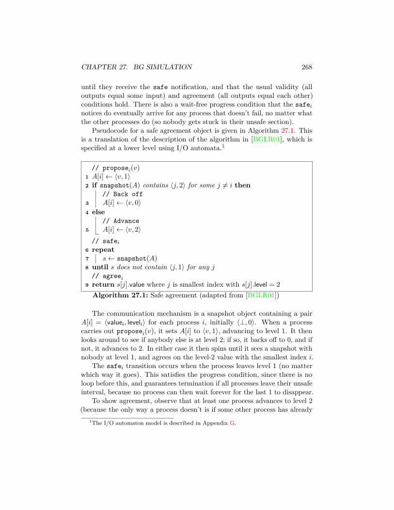
CHAPTER 27. BG SIMULATION 268

until they receive the safe notification, and that the usual validity (alloutputs equal some input) and agreement (all outputs equal each other)conditions hold. There is also a wait-free progress condition that the safeinotices do eventually arrive for any process that doesn’t fail, no matter whatthe other processes do (so nobody gets stuck in their unsafe section).

Pseudocode for a safe agreement object is given in Algorithm 27.1. Thisis a translation of the description of the algorithm in [BGLR01], which isspecified at a lower level using I/O automata.1

// proposei(v)1 A[i]← 〈v, 1〉2 if snapshot(A) contains 〈j, 2〉 for some j 6= i then

// Back off3 A[i]← 〈v, 0〉4 else

// Advance5 A[i]← 〈v, 2〉

// safei6 repeat7 s← snapshot(A)8 until s does not contain 〈j, 1〉 for any j

// agreei9 return s[j].value where j is smallest index with s[j].level = 2Algorithm 27.1: Safe agreement (adapted from [BGLR01])

The communication mechanism is a snapshot object containing a pairA[i] = 〈valuei, leveli〉 for each process i, initially 〈⊥, 0〉. When a processcarries out proposei(v), it sets A[i] to 〈v, 1〉, advancing to level 1. It thenlooks around to see if anybody else is at level 2; if so, it backs off to 0, and ifnot, it advances to 2. In either case it then spins until it sees a snapshot withnobody at level 1, and agrees on the level-2 value with the smallest index i.

The safei transition occurs when the process leaves level 1 (no matterwhich way it goes). This satisfies the progress condition, since there is noloop before this, and guarantees termination if all processes leave their unsafeinterval, because no process can then wait forever for the last 1 to disappear.

To show agreement, observe that at least one process advances to level 2(because the only way a process doesn’t is if some other process has already

1The I/O automaton model is described in Appendix G.

CHAPTER 27. BG SIMULATION 269

advanced to level 2), so any process i that terminates observes a snapshot sthat contains at least one level-2 tuple and no level-1 tuples. This meansthat any process j whose value is not already at level 2 in s can at worstreach level 1 after s is taken. But then j sees a level-2 tuples and backsoff. It follows that any other process i′ that takes a later snapshot s′ thatincludes no level-1 tuples sees the same level-2 tuples as i, and computes thesame return value. (Validity also holds, for the usual trivial reasons.)

27.3 The basic simulation algorithmThe basic BG simulation uses a single snapshot object A with t+1 componentsand an infinite array of safe agreement objects Sjr.

Each component A[i] of A belongs to one of the t+1 simulating processes,and is a vector of values A[i][j] that process i believes process j will havewritten at some point during the simulated execution. These values aretagged with round numbers: each A[i][j] holds a tuple 〈v, r〉 representing thevalue v that process i determines process j would have written after takingr snapshots.

The contents of these snapshots are obtained from the Sjr objects. Theinputs to Sjr are simulated snapshots, and the output sjr of Sjr representsthe value of the r-th snapshot performed by simulated process j.

Each simulating process i cycles through all simulated processes j. Simu-lating one round of a particular process j involves four phases:

1. Make an initial guess for sjr by taking a snapshot of A and taking thevalue with the largest round number for each component A[−][k].

2. Initiate the safe agreement protocol Sjr using this guess. It continuesto run Sjr until it leaves the unsafe interval.

3. Attempt to finish Sjr, by performing one iteration of the loop fromAlgorithm 27.1. If this iteration doesn’t succeed, move on to simulatingj + 1 (but come back to this phase for j eventually).

4. If Sjr terminates, compute a new value vjr for j to write based on thesimulated snapshot returned by Sjr, and update A[i][j] with 〈vjr, r〉.

Actually implementing this while maintaining an abstraction barrieraround safe agreement is tricky. One approach might be to have each processi manage a separate thread for each simulated process j, and wrap the unsafepart of the safe agreement protocol inside a mutex just for threads of i. This

CHAPTER 27. BG SIMULATION 270

guarantees that i enters the unsafe part of any safe agreement object onbehalf of only one simulated j at a time, while preventing delays in the safepart of Sjr from blocking it from finishing some other Sj′r′ .

27.4 Effect of failuresSo now what happens if a simulating process i fails? This won’t stop anyother process i′ from taking snapshots on behalf of j, or from generating itsown values to put in A[i′][j]. What it may do is prevent some safe agreementobject Sjr from terminating. The termination property of Sjr means thatthis can only occur if the failure occurs while i is in the unsafe interval forSjr—but since i is only in the unsafe interval for at most one Sjr at a time,this stalls only one simulated process j. It doesn’t block any i′, because anyother i′ is guaranteed to leave its own unsafe interval for Sjr after finitelymany steps, and though it may waste some effort waiting for Sjr to finish,once it is in the safe interval it doesn’t actually wait for it before moving onto other simulated j′.

It follows that each failure of a simulating process knocks out at mostone simulated process. So a wait-free system with t+ 1 processes—and thusat most t failures in the executions we care about—will produces at most tfailures inside the simulation.

27.5 Inputs and outputsTwo details not specified in the description above are how i determinesj’s initial input and how i determines its own outputs from the outputsof the simulated processes. For the basic BG simulation, this is prettystraightforward: we use the safe agreement objects Sj0 to agree on j’s input,after each i proposes its own input vector for all j based on its own input tothe simulator protocol. For outputs, i waits for at least n− t of the simulatedprocesses to finish, and computes its own output based on what it sees.

One issue that arises here is that we can only use the simulation tosolve colorless tasks, which are decision problems where any process canreturn the output of any other process without causing trouble.2 This worksfor consensus or k-set agreement, but fails pretty badly for renaming. Theextended BG simulation, due to Gafni [Gaf09], solves this problem by

2The term “colorless” here comes from use of colors to represent process ids in thetopological approach described in Chapter 28. These colors aren’t really colors, buttopologists like coloring nodes better than assigning them ids.

CHAPTER 27. BG SIMULATION 271

mapping each simulating process p to a specific simulated process qp, andusing a more sophisticated simulation algorithm to guarantee that qp doesn’tcrash unless p does; details can be found in Gafni’s paper. There is also alater paper by Imbs and Raynal [IR09] that simplifies some details of theconstruction. Here, we will limit ourselves to the basic BG simulation.

27.6 Correctness of the simulationTo show that the simulation works, observe that we can extract a simulatedexecution by applying the following rules:

1. The round-r write operation of j is represented by the first write taggedwith round r performed for j.

2. The round-r snapshot operation of j is represented by whichever snap-shot operation wins Sjr.

The simulated execution then consists of a sequence of write and snapshotoperations, with order of the operations determined by the order of theirrepresentatives in the simulating execution, and the return values of thesnapshots determined by the return values of their representatives.

Because all processes that simulate a write for j in round r use the samesnapshots to compute the state of j, they all write the same value. So the onlyway we get into trouble is if the writes included in our simulated snapshotsare inconsistent with the ordering of the simulated operations defined above.Here the fact that each simulated snapshot corresponds to a real snapshotmakes everything work: when a process performs a snapshot for Sjr, then itincludes all the simulated write operations that happen before this snapshot,since the s-th write operation by k will be represented in the snapshot if andonly if the first instance of the s-th write operation by k occurs before it.The only tricky bit is that process i’s snapshot for Sjr might include someoperations that can’t possibly be included in Sjr, like j’s round-r write orsome other operation that depends on it. But this can only occur if someother process finished Sjr before process i takes its snapshot, in which casei’s snapshot will not win Sjr and will be discarded.

27.7 BG simulation and consensusBG simulation was originally developed to attack k-set agreement, but (aspointed out by Gafni [Gaf09]) it gives a particularly simple proof of the

CHAPTER 27. BG SIMULATION 272

impossibility of consensus with one faulty process. Suppose that we had aconsensus protocol that solved consensus for n > 1 processes with one crashfailure, using only atomic registers. Then we could use BG simulation to geta wait-free consensus protocol for two processes. But it’s easy to show thatatomic registers can’t solve wait-free consensus, because (following [LAA87]),we only need to do the last step of FLP that gets a contradiction whenmoving from a bivalent C to 0-valent Cx or 1-valent Cy. We thus avoid thecomplications that arise in the original FLP proof from having to deal withfairness.

More generally, BG simulation means that increasing the number ofprocesses while keeping the same number of crash failures doesn’t let uscompute anything we couldn’t before. This gives a formal justification forthe slogan that the difference between distributed computing and parallelcomputing is that in a distributed system, more processes can only makethings worse.

Chapter 28

Topological methods

Here we’ll describe some results applying topology to distributed computing,mostly following a classic paper of Herlihy and Shavit [HS99]. This wasone of several papers [BG93, SZ00] that independently proved lower boundson k-set agreement [Cha93], which is a relaxation of consensus where werequire only that there are at most k distinct output values (consensus is1-set agreement). These lower bounds had failed to succumb to simplertechniques.

28.1 Basic ideaThe basic idea is to use tools from combinatorial topology to representindistinguishability proofs. We’ve seen a lot of indistinguishability proofs thatinvolving showing that particular pairs of executions are indistinguishable tosome process, which means that that process produces the same output inboth executions. In a typical proof of this kind, we then construct a chain ofexecutions Ξ1, . . . ,Ξk such that for each i, there is some p with Ξi|p = Ξi+1|p.We’ve generally been drawing these with the executions as points and theindistinguishability relation as an edge between two executions. In thetopological method, we use the dual of this picture: each process’s view (therestriction of some execution to events visible to that process) is representedas a point, and an execution Ξ is represented as a simplex connecting all ofthe points corresponding to views of Ξ by particular processes.

A simplex is a generalization to arbitrary dimension of the sequencethat starts with a point (a 0-simplex), an edge (a 1-simplex), a triangle(a 2-simplex), or a tetrahedron (a 3-simplex). In general, an n-simplex isa solid n-dimensional object with n + 1 vertices and n + 1 faces that are

273

CHAPTER 28. TOPOLOGICAL METHODS 274

(n− 1)-simplexes. As a combinatorial object, this is a fancy way of depictingthe power set of the set of vertices: each subset corresponds to a facet of theoriginal simplex. A simplicial complex consists of a bunch of simplexes pastedtogether by identifying vertices: this is similar to the technique in graphicsof representing the surface of a three-dimensional object by decomposingit into triangles. Topologists use these to model continuous surfaces, andhave many tools for deriving interesting properties of those surfaces from adescription of the simplicial complex.

For distributed computing, the idea is that some of these topological prop-erties, when computed for the simplicial complex resulting from some protocolor problem specification may sometimes useful to determine properties ofthe underlying protocol or problem.

28.2 k-set agreementThe motivating problem for much of this work was getting impossibilityresults for k-set agreement, proposed by Chaudhuri [Cha93]. The k-setagreement problem is similar to consensus, where each process starts withan input and eventually returns a decision value that must be equal to someprocess’s input, but the agreement condition is relaxed to require only thatthe set of decision values include at most k values.

With k − 1 crash failures, it’s easy to build a k-set agreement algorithm:wait until you have seen n− k+ 1 input values, then choose the smallest oneyou see. This works because any value a process returns is necessarily amongthe k smallest input values (including the k − 1 it didn’t see). Chaudhuriconjectured that k-set agreement was not solvable with k failures, and gavea proof of a partial result (analogous to the existence of an initial bivalentconfiguration for consensus) based on Sperner’s Lemma [Spe28]. This is aclassic result in topology that says that certain colorings of the vertices of agraph in the form of a triangle that has been divided into smaller trianglesnecessarily contain a small triangle with three different colors on its corners.This connection between k-set renaming and Sperner’s Lemma became thebasic idea behind each the three independent proofs of the conjecture thatappeared shortly thereafter [HS99, BG93, SZ00].

Our plan is to give a sufficient high-level description of the topologicalapproach that the connection between k-set agreement and Sperner’s Lemmabecomes obvious. It is possible to avoid this by approaching the problempurely combinatorially, as is done, for example, in Section 16.3 of [AW04].The presentation there is obtained by starting with a topological argument

CHAPTER 28. TOPOLOGICAL METHODS 275

and getting rid of the topology (in fact, the proof in [AW04] contains a proofof Sperner’s Lemma with the serial numbers filed off). The disadvantage ofthis approach is that it obscures what is really going in and makes it harder toobtain insight into how topological techniques might help for other problems.The advantage is that (unlike these notes) the resulting text includes actualproofs instead of handwaving.

28.3 Representing distributed computations usingtopology

Topology is the study of properties of shapes that are preserved by continuousfunctions between their points that have continuous inverses, which get therather fancy name of homeomorphisms. A continuous function1 is onethat maps nearby points to nearby points. A homeomorphism is continuousin both directions: this basically means that you can stretch and twist andotherwise deform your object however you like, as long as you don’t tearit (which would map nearby points on opposite sides of the tear to distantpoints) or glue bits of it together (which turns into tearing when we lookat the inverse function). Topologists are particularly interested in showingwhen there is no homeomorphism between two objects; the classic exampleis that you can’t turn a sphere into a donut without damaging it, but youcan turn a donut into a coffee mug (with a handle).

Working with arbitrary objects embedded in umpteen-dimensional spacesis messy, so topologists invented a finite way of describing certain well-behavedobjects combinatorially, by replacing ugly continuous objects like spheresand coffee mugs with simpler objects pasted together in complex ways. Thesimpler objects are simplexes, and the more complicated pasted-togetherobjects are called simplicial complexes. The nifty thing about simplicialcomplexes is that they give a convenient tool for describing what states oroutputs of processes in a distributed algorithm are “compatible” in somesense, and because topologists know a lot about simplicial complexes, wecan steal their tools to describe distributed algorithms.

1Strictly speaking, this is the definition a continuous function between metric spaces,which are spaces that have a consistent notion of distance. There is an even more generaldefinition of continuity that holds for spaces that are too strange for this.

CHAPTER 28. TOPOLOGICAL METHODS 276

28.3.1 Simplicial complexes and process states

The formal definition of a k-dimensional simplex is the convex closure of(k+1) points x1 . . . xk+1 in general position; the convex closure part meansthe set of all points

∑aixi where

∑ai = 1 and each ai ≥ 0, and the general

position part means that the xi are not all contained in some subspace ofdimension (k−1) or smaller (so that the simplex isn’t squashed flat somehow).What this gives us is a body with (k + 1) corners and (k + 1) faces, each ofwhich is a (k− 1)-dimensional simplex (the base case is that a 0-dimensionalsimplex is a point). Each face includes all but one of the corners, and eachcorner is on all but one of the faces. So we have:

• 0-dimensional simplex: point.2

• 1-dimensional simplex: line segment with 2 endpoints (which are bothcorners and faces).

• 2-dimensional simplex: triangle (3 corners with 3 1-dimensional sim-plexes for sides).

• 3-dimensional simplex: tetrahedron (4 corners, 4 triangular faces).

• 4-dimensional simplex: 5 corners, 5 tetrahedral faces. It’s probablybest not to try to visualize this.

A simplicial complex is a bunch of simplexes stuck together; formally,this means that we pretend that some of the corners (and any faces thatinclude them) of different simplexes are identical points. There are ways todo this right using equivalence relations. But it’s easier to abstract out theactual geometry and go straight to a combinatorial structure.

An (abstract) simplicial complex is just a collection of sets with theproperty that if A is a subset of B, and B is in the complex, then A is alsoin the complex (this means that if some simplex is included, so are all ofits faces, their faces, etc.). This combinatorial version is nice for reasoningabout simplicial complexes, but is not so good for drawing pictures.

The trick to using this for distributed computing problems is that weare going to build simplicial complexes by letting points be process states(or sometimes process inputs or outputs), each labeled with a process id,

2For consistency, it’s sometimes convenient to define a point as having a single (−1)-dimensional face defined to be the empty set. We won’t need to bother with this, since0-dimensional simplicial complexes correspond to 1-process distributed systems, which areamply covered in almost every other Computer Science class you have ever taken.

CHAPTER 28. TOPOLOGICAL METHODS 277

and letting the sets that appear in the complex be those collections ofstates/inputs/outputs that are compatible with each other in some sense.For states, this means that they all appear in some global configurationin some admissible execution of some system; for inputs and outputs, thismeans that they are permitted combinations of inputs or outputs in thespecification of some problem.

Example: For 2-process binary consensus with processes 0 and 1, theinput complex, which describes all possible combinations of inputs, consistsof the sets

, p0, q0, p1, q1, p0, q0, p0, q1, p1, q0, p1, q1 ,

which we might draw like this:

p0 q0

q1 p1

Note that there are no edges from p0 to p1 or q0 to q1: we can’t havetwo different states of the same process in the same global configuration.

The output complex, which describes the permitted outputs, is

, p0, q0, p1, q1, p0, q0, p1, q1 .

As a picture, this omits two of the edges (1-dimensional simplexes) from theinput complex:

p0 q0

q1 p1

One thing to notice about this output complex is that it is not connected:there is no path from the p0–q0 component to the q1–p1 component.

Here is a simplicial complex describing the possible states of two processesp and q, after each writes 1 to its own bit then reads the other process’s bit.Each node in the picture is labeled by a sequence of process ids. The first idin the sequence is the process whose view this node represents; any other

CHAPTER 28. TOPOLOGICAL METHODS 278

process ids are processes this first process sees (by seeing a 1 in the otherprocess’s register). So p is the view of process p running by itself, while pqis the view of process p running in an execution where it reads q’s registerafter q writes it.

p qp pq q

The edges express the constraint that if we both write before we read,then if I don’t see your value you must see mine (which is why there is nop–q edge), but all other combinations are possible. Note that this complexis connected: there is a path between any two points.

Here’s a fancier version in which each process writes its input (andremembers it), then reads the other process’s register (i.e., a one-round full-information protocol). We now have final states that include the process’sown id and input first, then the other process’s id and input if it is visible.For example, p1 means p starts with 1 but sees a null and q0p1 means q startswith 0 but sees p’s 1. The general rule is that two states are compatible if peither sees nothing or q’s actual input and similarly for q, and that at leastone of p or q must see the other’s input. This gives the following simplicialcomplex:

p0 q0p0 p0q0 q0

q1p0

p0q1

q1

p1q0

q0p1

p1q1 q1p1 p1

Again, the complex is connected.The fact that this looks like four copies of the p–qp–pq–q complex pasted

into each edge of the input complex is not an accident: if we fix a pair ofinputs i and j, we get pi–qjpi–piqj–qj, and the corners are pasted togetherbecause if p sees only p0 (say), it can’t tell if it’s in the p0/q0 execution orthe p0/q1 execution.

The same process occurs if we run a two-round protocol of this form,where the input in the second round is the output from the first round. Eachround subdivides one edge from the previous round into three edges:

CHAPTER 28. TOPOLOGICAL METHODS 279

p− q

p− qp− pq − q

p− (qp)p− p(qp)− qp− (pq)(qp)− (qp)(pq)− pq − q(pq)− (pq)q − q

Here (pq)(qp) is the view of p after seeing pq in the first round and seeingthat q saw qp in the first round.

28.3.2 Subdivisions

In the simple write-then-read protocol above, we saw a single input edge turninto 3 edges. Topologically, this is an example of a subdivision, where werepresent a simplex using several new simplexes pasted together that coverexactly the same points.

Certain classes of protocols naturally yield subdivisions of the inputcomplex. The iterated immediate snapshot (IIS) model, defined byBorowsky and Gafni [BG97], considers executions made up of a sequenceof rounds (the iterated part) where each round is made up of one or moremini-rounds in which some subset of the processes all write out their currentviews to their own registers and then take snapshots of all the registers (theimmediate snapshot part). The two-process protocols of the previous sectionare special cases of this model.

Within each round, each process p obtains a view vp that contains theprevious-round views of some subset of the processes. We can represent theviews as a subset of the processes, which we will abbreviate in pictures byputting the view owner first: pqr will be the view p, q, r as seen by p, whileqpr will be the same view as seen by q. The requirements on these viewsare that (a) every process sees its own previous view: p ∈ vp for all p; (b)all views are comparable: vp ⊆ vq or vq ⊆ vp; and (c) if I see you, then I seeeverything you see: q ∈ vp implies vq ⊆ vp. This last requirement is calledimmediacy and follows from the assumption that writes and snapshots aredone in the same mini-round: if I see your write, then I see all the valuesyou do, because your snapshot is either in an earlier mini-round than mineor in the same mini-round. Note this depends on the peculiar structure ofthe mini-rounds, where all the writes precede all the snapshots.

CHAPTER 28. TOPOLOGICAL METHODS 280

The IIS model does not correspond exactly to a standard shared-memorymodel (or even a standard shared-memory model augmented with cheapsnapshots). There are two reasons for this: standard snapshots don’t provideimmediacy, and standard snapshots allow processes to go back and performmore than one snapshot on the same object. The first issue goes away ifwe are looking at impossibility proofs, because the adversary can restrictitself only to those executions that satisfy immediacy; alternatively, we canget immediacy from the participating set protocol of [BG97], which wewill describe in §28.6.1. The second issue is more delicate, but Borowskyand Gafni demonstrate that any decision protocol that runs in the standardmodel can be simulated in the IIS model, using a variant of the BG simulationalgorithm described in Chapter 27.

For three processes, one round of immediate snapshots gives rise to thesimplicial complex depicted in Figure 28.1. The corners of the big triangleare the solo views of processes that do their snapshots before anybody elseshows up. Along the edges of the big triangle are views corresponding to2-process executions, while in the middle are complete views of processes thatrun late enough to see everything. Each little triangle corresponds to someexecution. For example, the triangle with corners p, qp, rpq corresponds toa sequential execution where p sees nobody, q sees p, and r sees both p andq. The triangle with corners pqr, qpr, and rpq is the maximally-concurrentexecution where all three processes write before all doing their snapshots:here everybody sees everybody. It is not terribly hard to enumerate allpossible executions and verify that the picture includes all of them. In higherdimension, the picture is more complicated, but we still get a subdivisionthat preserves the original topological structure [BG97].

Figure 28.2 shows (part of) the next step of this process: here we havedone two iterations of immediate snapshot, and filled in the second-roundsubdivisions for the p–qpr–rpq and pqr–qpr–rpq triangles. (Please imaginesimilar subdivisions of all the other triangles that I was too lazy to fill inby hand.) The structure is recursive, with each first-level triangle mappingto an image of the entire first-level complex. As in the two-process case,adjacent triangles overlap because the relevant processes don’t have enoughinformation; for example, the points on the qpr–rpq edge correspond to viewsof q or r that don’t include p in round 2 and so can’t tell whether p saw p orpqr in round 1.

The important feature of the round-2 complex (and the round-k complexin general) is that it’s a triangulation of the original outer triangle: apartition into little triangles where each corner aligns with corners of otherlittle triangles.

CHAPTER 28. TOPOLOGICAL METHODS 281

p

qr

rpq

qp

pq

rqqr

qpr

pqr

pr

rp

Figure 28.1: Subdivision corresponding to one round of immediate snapshot

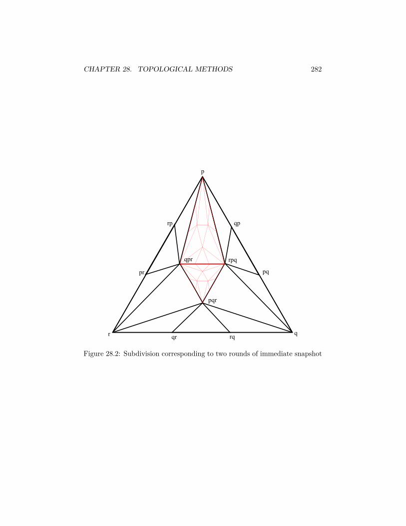
CHAPTER 28. TOPOLOGICAL METHODS 282

p

qr

rpq

qp

pq

rqqr

qpr

pqr

pr

rp

Figure 28.2: Subdivision corresponding to two rounds of immediate snapshot

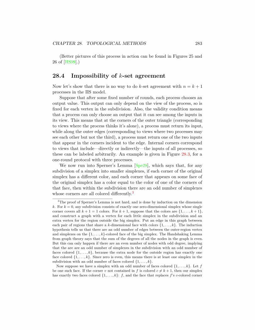
CHAPTER 28. TOPOLOGICAL METHODS 283

(Better pictures of this process in action can be found in Figures 25 and26 of [HS99].)

28.4 Impossibility of k-set agreementNow let’s show that there is no way to do k-set agreement with n = k + 1processes in the IIS model.

Suppose that after some fixed number of rounds, each process chooses anoutput value. This output can only depend on the view of the process, so isfixed for each vertex in the subdivision. Also, the validity condition meansthat a process can only choose an output that it can see among the inputs inits view. This means that at the corners of the outer triangle (correspondingto views where the process thinks it’s alone), a process must return its input,while along the outer edges (corresponding to views where two processes maysee each other but not the third), a process must return one of the two inputsthat appear in the corners incident to the edge. Internal corners correspondto views that include—directly or indirectly—the inputs of all processes, sothese can be labeled arbitrarily. An example is given in Figure 28.3, for aone-round protocol with three processes.

We now run into Sperner’s Lemma [Spe28], which says that, for anysubdivision of a simplex into smaller simplexes, if each corner of the originalsimplex has a different color, and each corner that appears on some face ofthe original simplex has a color equal to the color of one of the corners ofthat face, then within the subdivision there are an odd number of simplexeswhose corners are all colored differently.3

3The proof of Sperner’s Lemma is not hard, and is done by induction on the dimensionk. For k = 0, any subdivision consists of exactly one zero-dimensional simplex whose singlecorner covers all k + 1 = 1 colors. For k + 1, suppose that the colors are 1, . . . , k + 1,and construct a graph with a vertex for each little simplex in the subdivision and anextra vertex for the region outside the big simplex. Put an edge in this graph betweeneach pair of regions that share a k-dimensional face with colors 1, . . . , k. The inductionhypothesis tells us that there are an odd number of edges between the outer-region vertexand simplexes on the 1, . . . , k-colored face of the big simplex. The Handshaking Lemmafrom graph theory says that the sum of the degrees of all the nodes in the graph is even.But this can only happen if there are an even number of nodes with odd degree, implyingthat the are are an odd number of simplexes in the subdivision with an odd number offaces colored 1, . . . , k, because the extra node for the outside region has exactly oneface colored 1, . . . , k. Since zero is even, this means there is at least one simplex in thesubdivision with an odd number of faces colored 1, . . . , k.

Now suppose we have a simplex with an odd number of faces colored 1, . . . , k. Let fbe one such face. If the corner v not contained in f is colored c 6= k + 1, then our simplexhas exactly two faces colored 1, . . . , k: f , and the face that replaces f ’s c-colored corner

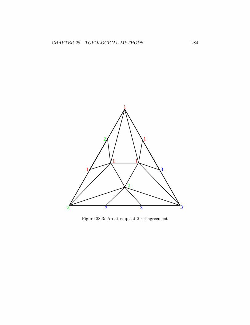
CHAPTER 28. TOPOLOGICAL METHODS 284

1

2 3

1

1

1 1

3

3

2

3

2

Figure 28.3: An attempt at 2-set agreement

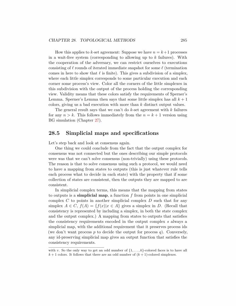
CHAPTER 28. TOPOLOGICAL METHODS 285

How this applies to k-set agreement: Suppose we have n = k+1 processesin a wait-free system (corresponding to allowing up to k failures). Withthe cooperation of the adversary, we can restrict ourselves to executionsconsisting of ` rounds of iterated immediate snapshot for some ` (terminationcomes in here to show that ` is finite). This gives a subdivision of a simplex,where each little simplex corresponds to some particular execution and eachcorner some process’s view. Color all the corners of the little simplexes inthis subdivision with the output of the process holding the correspondingview. Validity means that these colors satisfy the requirements of Sperner’sLemma. Sperner’s Lemma then says that some little simplex has all k + 1colors, giving us a bad execution with more than k distinct output values.

The general result says that we can’t do k-set agreement with k failuresfor any n > k. This follows immediately from the n = k + 1 version usingBG simulation (Chapter 27).

28.5 Simplicial maps and specificationsLet’s step back and look at consensus again.

One thing we could conclude from the fact that the output complex forconsensus was not connected but the ones describing our simple protocolswere was that we can’t solve consensus (non-trivially) using these protocols.The reason is that to solve consensus using such a protocol, we would needto have a mapping from states to outputs (this is just whatever rule tellseach process what to decide in each state) with the property that if somecollection of states are consistent, then the outputs they are mapped to areconsistent.

In simplicial complex terms, this means that the mapping from statesto outputs is a simplicial map, a function f from points in one simplicialcomplex C to points in another simplicial complex D such that for anysimplex A ∈ C, f(A) = f(x)|x ∈ A gives a simplex in D. (Recall thatconsistency is represented by including a simplex, in both the state complexand the output complex.) A mapping from states to outputs that satisfiesthe consistency requirements encoded in the output complex s always asimplicial map, with the additional requirement that it preserves process ids(we don’t want process p to decide the output for process q). Conversely,any id-preserving simplicial map gives an output function that satisfies theconsistency requirements.

with v. So the only way to get an odd number of 1, . . . , k-colored faces is to have allk + 1 colors. It follows that there are an odd number of (k + 1)-colored simplexes.

CHAPTER 28. TOPOLOGICAL METHODS 286

Simplicial maps are examples of continuous functions, which have allsorts of nice topological properties. One nice property is that a continuousfunction can’t separate a path-connected space ( one in which there is apath between any two points) into path-disconnected components. We canprove this directly for simplicial maps: if there is a path of 1-simplexesx1, x2, x2, x3, . . . xk−1, xk from x1 to xk in C, and f : C → D is asimplicial map, then there is a path of 1-simplexes f(x1), f(x2), . . . fromf(x1) to f(xk). Since being path-connected just means that there is a pathbetween any two points, if C is connected we’ve just shown that f(C) is aswell.

Getting back to our consensus example, it doesn’t matter what simplicialmap f you pick to map process states to outputs; since the state complex Cis connected, so is f(C), so it lies entirely within one of the two connectedcomponents of the output complex. This means in particular that everybodyalways outputs 0 or 1: the protocol is trivial.

28.5.1 Mapping inputs to outputs

For general decision tasks, it’s not enough for the outputs to be consistentwith each other. They also have to be consistent with the inputs. This canbe expressed by a relation ∆ between input simplexes and output simplexes.

Formally, a decision task is modeled by a triple (I,O,∆), where I is theinput complex, O is the output complex, and (A,B) ∈ ∆ if and only if B isa permissible output given input I. Here there are no particular restrictionson ∆ (for example, it doesn’t have to be a simplicial map or even a function),but it probably doesn’t make sense to look at decision tasks unless there isat least one permitted output simplex for each input simplex.

28.6 The asynchronous computability theoremGiven a decision task specified in this way, there is a topological characteriza-tion of when it has a wait-free solution. This is given by the AsynchronousComputability Theorem (Theorem 3.1 in [HS99]), which says:

Theorem 28.6.1. A decision task (I,O,∆) has a wait-free protocol usingshared memory if and only if there exists a chromatic subdivision σ of I anda color-preserving simplicial map µ : σ(I)→ O such that for each simplex sin σ(I), µ(S) ∈ ∆(carrier(S, I)).

To unpack this slightly, a chromatic subdivision is a subdivision whereeach vertex is labeled by a process id (a color), and no simplex has two

CHAPTER 28. TOPOLOGICAL METHODS 287

vertices with the same color. A color-preserving simplicial map is a simplicialmap that preserves ids. The carrier of a simplex in a subdivision is whateveroriginal simplex it is part of. So the theorem says that I can only solve atask if I can find a simplicial map from a subdivision of the input complexto the output complex that doesn’t do anything strange to process ids andthat is consistent with ∆.

Looking just at the theorem, one might imagine that the proof consistsof showing that the protocol complex defined by the state complex afterrunning the protocol to completion is a subdivision of the input complex,followed by the same argument we’ve seen already about mapping the statecomplex to the output complex. This is almost right, but it’s complicated bytwo inconvenient facts: (a) the state complex generally isn’t a subdivision ofthe input complex, and (b) if we have a map from an arbitrary subdivisionof the input complex, it is not clear that there is a corresponding protocolthat produces this particular subdivision.

So instead the proof works like this:

Protocol implies map Even though we don’t get a subdivision with thefull protocol, there is a restricted set of executions that does give asubdivision. So if the protocol works on this restricted set of execu-tions, an appropriate map exists. There are two ways to prove this:Herlihy and Shavit do so directly, by showing that this restricted setof executions exists, and Borowksy and Gafni [BG97] do so indirectly,by showing that the IIS model (which produces exactly the standardchromatic subdivision used in the ACT proof) can simulate an ordinarysnapshot model. Both methods are a bit involved, so we will skip overthis part.

Map implies protocol This requires an algorithm. The idea here is thatthat participating set algorithm, originally developed to solve k-setagreement [BG93], produces precisely the standard chromatic subdivi-sion used in the ACT proof. In particular, it can be used to solve theproblem of simplex agreement, the problem of getting the processesto agree on a particular simplex contained within the subdivision oftheir original common input simplex. This is a little easier to explain,so we’ll do it.

28.6.1 The participating set protocol

Algorithm 28.1 depicts the participating set protocol; this first appearedin [BG93], although the presentation here is heavily influenced by the version

CHAPTER 28. TOPOLOGICAL METHODS 288

in Elizabeth Borowsky’s dissertation [Bor95]. The shared data consists ofa snapshot object level, and processes start at a high level and float downuntil they reach a level i such that there are already i processes at this levelor below. The set returned by a process consists of all processes it sees atits own level or below, and it can be shown that this in fact implements aone-shot immediate snapshot. Since immediate snapshots yield a standardsubdivision, this gives us what we want for converting a color-preservingsimplicial map to an actual protocol.

1 Initially, level[i] = n+ 2 for all i.2 repeat3 level[i]← level[i]− 14 v ← snapshot(level)5 S ← j | v[j] ≤ level[i]6 until |S| ≥ level[i]7 return S

Algorithm 28.1: Participating set

The following theorem shows that the return values from participatingset have all the properties we want for iterated immediate snapshot:

Theorem 28.6.2. Let Si be the output of the participating set algorithm forprocess i. Then all of the following conditions hold:

1. For all i, i ∈ Si. (Self-containment.)

2. For all i, j, Si ⊆ Sj or Sj ⊆ Si. (Atomic snapshot.)

3. For all i, j, if i ∈ Sj, then Si ⊆ Sj. (Immediacy.)

Proof. Self-inclusion is trivial, but we will have to do some work for the othertwo properties.

The first step is to show that Algorithm 28.1 neatly sorts the processesout into levels, where each process that returns at level ` returns preciselythe set of processes at level ` and below.

For each process i, let Si be the set of process ids that i returns, let `ibe the final value of level[i] when i returns, and let S′i = j | `j ≤ `i. Ourgoal is to show that S′i = Si, justifying the above claim.

Because no process ever increases its level, if process i observes level[j] ≤ `iin its last snapshot, then `j ≤ level[j] ≤ `i. So S′i is a superset of Si. Wethus need to show only that no extra processes sneak in; in particular, wewill to show that |Si| = |S′i|, by showing that both equal `i.

CHAPTER 28. TOPOLOGICAL METHODS 289

The first step is to show that |S′i| ≥ |Si| ≥ `i. The first inequality followsfrom the fact that S′i ⊇ Si; the second follows from the code (if not, i wouldhave stayed in the loop).

The second step is to show that |S′i| ≤ `i. Suppose not; that is, supposethat |S′i| > `i. Then there are at least `i + 1 processes with level `i or less, allof which take a snapshot on level `i + 1. Let i′ be the last of these processesto take a snapshot while on level `i + 1. Then i′ sees at least `i + 1 processesat level `i + 1 or less and exits, contradicting the assumption that it reacheslevel `i. So |S′i| ≤ `i.

The atomic snapshot property follows immediately from the fact that if`i ≤ `j , then `k ≤ `i implies `k ≤ `j , giving Si = S′i ⊆ S′j = Sj . Similarly, forimmediacy we have that if i ∈ Sj , then `i ≤ `j , giving Si ≤ Sj by the sameargument.

The missing piece for turning this into IIS is that in Algorithm 28.1, Ionly learn the identities of the processes I am supposed to include but nottheir input values. This is easily dealt with by the usual trick of adding anextra register for each process, to which it writes its input before executingparticipating set.

28.7 Proving impossibility resultsTo show something is impossible using the ACT, we need to show thatthere is no color-preserving simplicial map from a subdivision of I to Osatisfying the conditions in ∆. This turns out to be equivalent to showingthat there is no continuous function from I to O with the same properties,because any such simplicial map can be turned into a continuous function(on the geometric version of I, which includes the intermediate points inaddition to the corners). Fortunately, topologists have many tools for provingnon-existence of continuous functions.

28.7.1 k-connectivity

Define the m-dimensional disk to be the set of all points at most 1 unit awayfrom the origin in Rm, and the m-dimensional sphere to be the surface ofthe (m+ 1)-dimensional disk (i.e., all points exactly 1 unit away from theorigin in Rm+1). Note that what we usually think of as a sphere (a solidbody), topologists call a disk, leaving the term sphere for just the outsidepart.

CHAPTER 28. TOPOLOGICAL METHODS 290

An object is k-connected if any continuous image of an m-dimensionalsphere can be extended to a continuous image of an (m + 1)-dimensionaldisk, for all m ≤ k.4 This is a roundabout way of saying that if we can drawsomething that looks like a deformed sphere inside our object, we can alwaysinclude the inside as well: there are no holes that get in the way. The punchline is that continuous functions preserve k-connectivity: if we want to mapan object with no holes continuously into some other object, the image hadbetter not have any holes either.

Ordinary path-connectivity is the special case when k = 0; here, the0-sphere consists of two points and the 1-disk is the path between them. So0-connectivity says that for any two points, there is a path between them.

For 1-connectivity, if we draw a loop (a path that returns to its origin),we can include the interior of the loop somewhere. One way to thinkingabout this is to say that we can shrink the loop to a point without leavingthe object (the technical term for this is that the path is null-homotopic,where a homotopy is a way to transform one thing continuously into anotherthing over time and the null path sits on a single point). An object that is1-connected is also called simply connected.

For 2-connectivity, we can’t contract a sphere (or box, or the surface of a2-simplex, or anything else that looks like a sphere) to a point.

The important thing about k-connectivity is that it is possible to provethat any subdivision of a k-connected simplicial complex is also k-connected(sort of obvious if you think about the pictures, but it can also be provedformally), and that k-connectivity is preserved by simplicial maps (if not,somewhere in the middle of all the k-simplexes representing our surface is a(k+ 1)-simplex in the domain that maps to a hole in the range, violating therule that simplicial maps map simplexes to simplexes). So a quick way toshow that the Asynchronous Computability Theorem implies that somethingis not asynchronously computable is to show that the input complex isk-connected and the output complex isn’t.

28.7.2 Impossibility proofs for specific problems

Here are some applications of the Asynchronous Computability Theoremand k-connectivity:

Consensus There is no nontrivial wait-free consensus protocol for n ≥ 24This definition is for the topological version of k-connectivity. It is not related in any

way to the definition of k-connectivity in graph theory, where a graph is k-connected ifthere are k disjoint paths between any two points.

CHAPTER 28. TOPOLOGICAL METHODS 291

a1 b2

c3 a4

c1

b1 c2

b3

a2

c4

b1

a1

a3

b2

c2

c1

b4

a1

a2

c3

b1

Figure 28.4: Output complex for renaming with n = 3, m = 4. Each vertexis labeled by a process id (a, b, c) and a name (1, 2, 3, 4). Observe that theleft and right edges of the complex have the same sequence of labels, as dothe top and bottom edges; the complex thus folds up into a (twisted) torus.(This is a poor imitation of part of [HS99, Figure 9].)

processes. Proof: The input complex is 1-connected, but the outputcomplex is not, and we need a map that covers the entire outputcomplex (by nontriviality).

k-set agreement There is no wait-free k-set agreement for n ≥ k + 1processes. Proof: The output complex for k-set agreement is notk-connected, because buried inside it are lots of (k + 1)-dimensionalholes corresponding to missing simplexes where all k + 1 processeschoose different values. But these holes aren’t present in the inputcomplex—it’s OK if everybody starts with different inputs—and thevalidity requirements for k-set agreement force us to map the surfacesof these non-holes around holes in the output complex. (This proofactually turns into the Sperner’s Lemma proof if we fully expand theclaim about having to map the input complex around the hole.)

Renaming There is no wait-free renaming protocol with less than 2n− 1output names for all n. The general proof of this requires showing thatwith fewer names we get holes that are too big (and ultimately reducesto Sperner’s Lemma); for the special case of n = 3 and m = 4, seeFigure 28.4, which shows how the output complex of renaming foldsup into the surface of a torus. This means that renaming for n = 3and m = 4 is exactly the same as trying to stretch a basketball into aninner tube.

Chapter 29

Approximate agreement

Last updated 2011. Some material may be out of date.

The approximate agreement [DLP+86] or ε-agreement problem isanother relaxation of consensus where input and output values are realnumbers, and a protocol is required to satisfy modified validity and agreementconditions.

Let xi be the input of process i and yi its output. Then a protocolsatisfies approximate agreement if it satisfies:

Termination Every nonfaulty process eventually decides.

Validity Every process returns an output within the range of inputs. For-mally, for all i, it holds that (minj xj) ≤ yi ≤ (maxj xj).

ε-agreement For all i and j, |i− j| ≤ ε.

Unlike consensus, approximate agreement has wait-free algorithms forasynchronous shared memory, which we’ll see in §29.1). But a curiousproperty of approximate agreement is that it has no bounded wait-freealgorithms, even for two processes (see §29.2)

29.1 Algorithms for approximate agreementNot only is approximate agreement solvable, it’s actually easily solvable, tothe point that there are many known algorithms for solving it.

292

CHAPTER 29. APPROXIMATE AGREEMENT 293

We’ll use the algorithm of Moran [Mor95], mostly as presented in [AW04,Algorithm 54] but with a slight bug fix;1 pseudocode appears in Algo-rithm 29.1.2

The algorithm carries out a sequence of asynchronous rounds in whichprocesses adopt new values, such that the spread of the vector of all valuesVr in round r, defined as spreadVr = max Vr −minVr, drops by a factor of2 per round. This is done by having each process choose a new value in eachround by taking the midpoint (average of min and max) of all the values itsees in the previous round. Slow processes will jump to the maximum roundthey see rather than propagating old values up from ancient rounds; this isenough to guarantee that latecomer values that arrive after some processwrites in round 2 are ignored.

The algorithm uses a single snapshot object A to communicate, andeach process stores its initial input and a round number along with itscurrent preference. We assume that the initial values in this object all haveround number 0, and that log2 0 = −∞ (which avoids a special case in thetermination test).

1 A[i]← 〈xi, 1, xi〉2 repeat3 〈x′1, r1, v1〉 . . . 〈x′n, rn, vn〉 ← snapshot(A)4 rmax ← maxj rj5 v ← midpointvj | rj = rmax6 A[i]← 〈xi, rmax + 1, v〉7 until rmax ≥ 2 and rmax ≥ log2(spread(x′j)/ε)8 return v

Algorithm 29.1: Approximate agreement

To show this works, we want to show that the midpoint operationguarantees that the spread shrinks by a factor of 2 in each round. Let Vr

1The original algorithm from [AW04] does not include the test rmax ≥ 2. This allowsfor bad executions in which process 1 writes its input of 0 in round 1 and takes a snapshotthat includes only its own input, after which process 2 runs the algorithm to completionwith input 1. Here process 2 will see 0 and 1 in round 1, and will write (1/2, 2, 1) toA[2]; on subsequent iterations, it will see only the value 1/2 in the maximum round, andafter dlog2(1/ε)e rounds it will decide on 1/2. But if we now wake process 1 up, it willdecided 0 immediately based on its snapshot, which includes only its own input and givesspread(x) = 0. Adding the extra test prevents this from happening, as new values thatarrive after somebody writes round 2 will be ignored.

2Showing that this particular algorithm works takes a lot of effort. If I were to do thisover, I’d probably go with a different algorithm due to Schenk [Sch95].

CHAPTER 29. APPROXIMATE AGREEMENT 294

be the set of all values v that are ever written to the snapshot object withround number r. Let Ur ⊆ Vr be the set of values that are ever written tothe snapshot object with round number r before some process writes a valuewith round number r+1 or greater; the intuition here is that Ur includes onlythose values that might contribute to the computation of some round-(r + 1)value.

Lemma 29.1.1. For all r for which Vr+1 is nonempty,

spread(Vr+1) ≤ spread(Ur)/2.

Proof. Let U ir be the set of round-r values observed by a process i in theiteration in which it sees rmax = r in some iteration, if such an iterationexists. Note that U ir ⊆ Ur, because if some value with round r+ 1 or greateris written before i’s snapshot, then i will compute a larger value for rmax.

Given two processes i and j, we can argue from the properties of snapshotthat either U ir ⊆ U jr or U jr ⊆ U ir. The reason is that if i’s snapshot comesfirst, then j sees at least as many round-r values as i does, because the onlyway for a round-r value to disappear is if it is replaced by a value in a laterround. But in this case, process j will compute a larger value for rmax andwill not get a view for round r. The same holds in reverse if j’s snapshotcomes first.

Observe that if U ir ⊆ U jr , then∣∣∣midpoint(U ir)−midpoint(U jr )∣∣∣ ≤ spread(U jr )/2.

This holds because midpoint(U ir) lies within the interval[minU jr ,maxU jr

],

and every point in this interval is within spread(U jr )/2 of midpoint(U jr ). Thesame holds if U jr ⊆ U ir. So any two values written in round r + 1 are withinspread(Ur)/2 of each other.

In particular, the minimum and maximum values in Vr+1 are withinspread(Ur)/2 of each other, so spread(Vr+1) ≤ spread(Ur)/2.

Corollary 29.1.2. For all r ≥ 2 for which Vr is nonempty,

spread(Vr) ≤ spread(U1)/2r−1.

Proof. By induction on r. For r = 2, this is just Lemma 29.1.1. For largerr, use the fact that Ur−1 ⊆ Vr−1 and thus spread(Ur−1) ≤ spread(Vr−1) to

CHAPTER 29. APPROXIMATE AGREEMENT 295

compute

spread(Vr) ≤ spread(Ur−1)/2≤ spread(Vr−1)/2≤ (spread(U1)/2r−2)/2= spread(U1)/2r−1.

Let i be some process that finishes in the fewest number of rounds. Processi can’t finish until it reaches round rmax+1, where rmax ≥ log2(spread(x′j)/ε)for a vector of input values x′ that it reads after some process writes round2 or greater. We have spread(x′j) ≥ spread(U1), because every value inU1 is included in x′. So rmax ≥ log2 (spread(U1)/ε) and spread(Vrmax+1) ≤spread(U1)/2rmax ≤ spread(U1)/(spread(U1)/ε) = ε. Since any value re-turned is either included in Vrmax+1 or some later Vr′ ⊆ Vrmax+1, this givesus that the spread of all the outputs is less than ε: Algorithm 29.1 solvesapproximate agreement.

The cost of Algorithm 29.1 depends on the cost of the snapshot operations,on ε, and on the initial input spread D. For linear-cost snapshots, this worksout to O(n log(D/ε)).

29.2 Lower bound on step complexityThe dependence on D/ε is necessary, at least for deterministic algorithms.Here we give a lower bound due to Herlihy [Her91a], which shows that anydeterministic approximate agreement algorithm takes at least log3(D/ε) totalsteps even with just two processes.

Define the preference of a process in some configuration as the value itwill choose if it runs alone starting from this configuration. The preferenceof a process p is well-defined because the process is deterministic; it also canonly change as a result of a write operation by another process q (becauseno other operations are visible to p, and p’s own operations can’t changeits preference). The validity condition means that in an initial state, eachprocess’s preference is equal to its input.

Consider an execution with two processes p and q, where p starts withpreference p0 and q starts with preference q0. Run p until it is about toperform a write that would change q’s preference. Now run q until it is aboutto change p’s preference. If p’s write no longer changes q’s preference, start p

CHAPTER 29. APPROXIMATE AGREEMENT 296

again and repeat until both p and q have pending writes that will change theother process’s preference. Let p1 and q1 be the new preferences that resultfrom these operations. The adversary can now choose between running P onlyand getting to a configuration with preferences p0 and q1, Q only and gettingp1 and q0, or both and getting p1 and q1; each of these choices incurs at leastone step. By the triangle inequality, |p0 − q0| ≤ |p0 − q1|+|q1 − p1|+|p1 − q0|,so at least on of these configurations has a spread between preferences that isat least 1/3 of the initial spread. It follows that after k steps the best spreadwe can get is D/3k, requiring k ≥ log3(D/ε) steps to get ε-agreement.

Herlihy uses this result to show that there are decisions problems that havewait-free but not bounded wait-free deterministic solutions using registers.Curiously, the lower bound says nothing about the dependence on the numberof processes; it is conceivable that there is an approximate agreement protocolwith running time that depends only on D/ε and not n.

Part III

Other communication models

297

Chapter 30

Overview

In this part, we consider models that don’t fit well into the standard message-passing or shared-memory models. These includes models where processescan directly observe the states of nearby processes (Chapter 31); wherecomputation is inherently local and the emphasis is on computing informationabout the communication graph (Chapter 32); where processes wander aboutand exchange information only with processes they physically encounter(Chapter 33); where processes (in the form of robots) communicate only byobserving each others’ locations and movements (Chapter 34); and whereprocesses can transmit only beeps, and are able to observe only whether atleast one nearby process beeped (Chapter 35).

Despite the varying communication mechanisms, these models all sharethe usual features of distributed systems, where processes must contend withnondeterminism and incomplete local information.

298

Chapter 31

Self-stabilization

A self-stabilizing algorithm has the property that, starting from any ar-bitrary configuration, it eventually reaches a legal configuration, and thisproperty is stable in the sense that it remains in a legal configurationthereafter. The notion of which configurations are legal depends on whatproblem we are trying to solve, but the overall intuition is that an algorithmis self-stabilizing if it can recover from arbitrarily horrible errors, and willstay recovered as long as no new errors occur.

It’s generally not possible to detect whether the algorithm is in a legalconfiguration from the inside: if a process has a bit that says that everythingis OK, the adversary can set that bit in the initial configuration, even ifeverything is in fact broken. So self-stabilizing algorithms don’t actuallyterminate: at best, they eventually converge to a configuration where thenecessary ongoing paranoid consistency checks produce no further changesto the configuration (a property called silent self-stabilization.

The idea of self-stabilization first appeared in a paper by Edsger Dijk-stra [Dij74], where he considered the problem of building robust token-ringnetworks. In a token-ring network, there are n nodes arranged in a directedcycle, and we want a single token to circulate through the nodes, as a mech-anism for enforcing mutual exclusion: only the node currently possessing thetoken can access the shared resource.

The problem is: how do you get the token started? Dijkstra worried bothabout the possibility of starting with no tokens or with more than one token,and he wanted an algorithm that would guarantee that, from any startingstate, eventually we would end up with exactly one token that would circulateas desired. He called such an algorithm self-stabilizing, and gave threeexamples, the simplest of which we will discuss in §31.2 below. These became

299

CHAPTER 31. SELF-STABILIZATION 300

the foundation for the huge field of self-stabilization, which spans thousandsof papers, at least one textbook [Dol00], a specialized conference (SSS, theInternational Symposium on Stabilization, Safety, and Security in DistributedSystems), and its own domain name http://www.selfstabilization.org/.We won’t attempt to summarize all of this, but will highlight a few resultsto give a sampling of what self-stabilizing algorithms look like.

31.1 ModelMuch of the work in this area, dating back to Dijkstra’s original paper, doesnot fit well in either the message-passing or shared-memory models that wehave been considering in this class, both of which were standardized muchlater. Instead, Dijkstra assumed that processes could, in effect, directlyobserve the states of their neighbors. A self-stabilizing program wouldconsist of a collection of what he later called guarded commands [Dij75],statements of the form “if [some condition is true] then [update my state inthis way].” In any configuration of the system, one or more of these guardedcommands might have the if part (the guard) be true; these commands aresaid to be enabled.

A step consists of one or more of these enabled commands being executedsimultaneously, as chosen by an adversary scheduler, called the distributeddaemon. The usual fairness condition applies: any process that has anenabled command eventually gets to execute it. If no commands are enabled,nothing happens. With the central daemon variant of the model, only onestep can happen at a time. With the synchronous daemon, every enabledstep happens at each time. Note that both the central and synchronousdaemons are special cases of the distributed daemon.

More recent work has tended to assume a distinction between the partof a process’s state that is visible to its neighbors and the part that isn’t.This usually takes the form of explicit communication registers or linkregisters, which allow a process to write a specific message for a specificneighbor. This is still not quite the same as standard message-passing orshared-memory, because a process is often allowed to read and write multiplelink registers atomically.

31.2 Token ring circulationFor example, let us consider Dijkstra’s token ring circulation algorithm.There are several versions of this in Dijkstra’s paper [Dij74]. We will do the

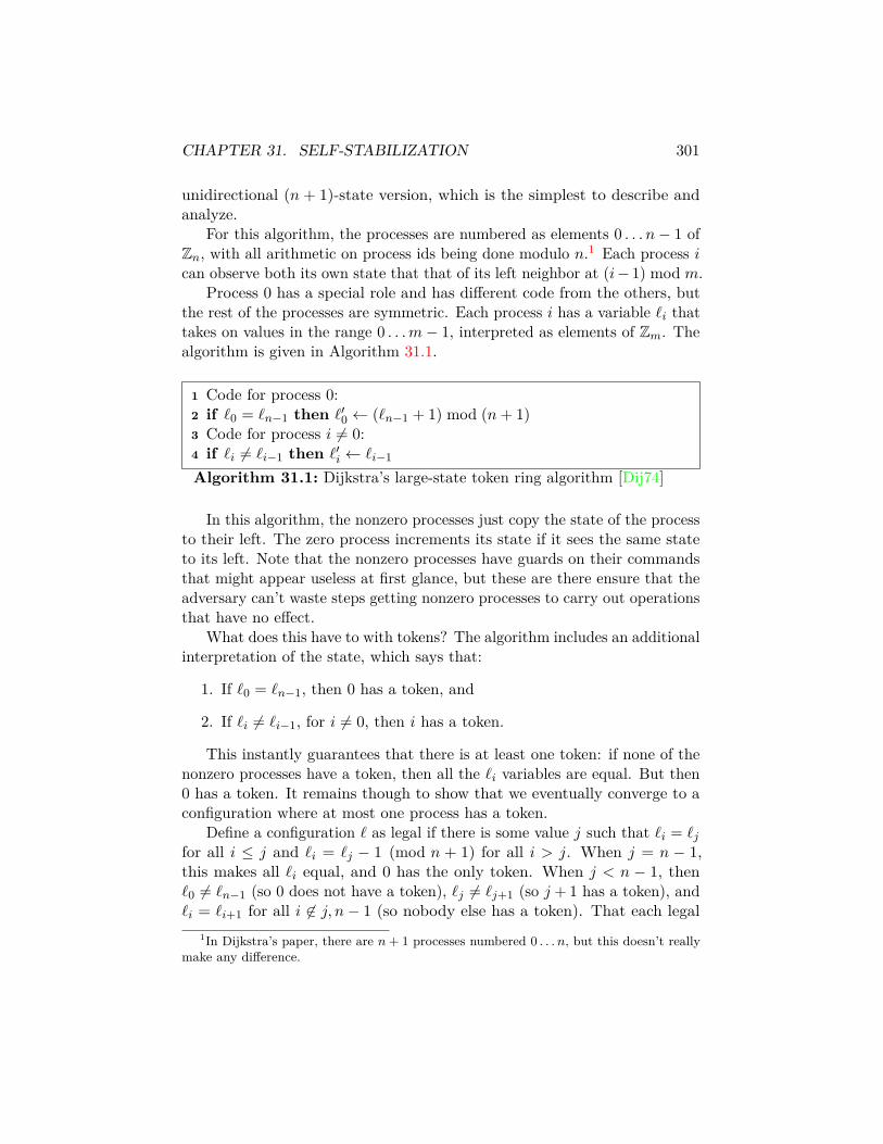
CHAPTER 31. SELF-STABILIZATION 301

unidirectional (n + 1)-state version, which is the simplest to describe andanalyze.

For this algorithm, the processes are numbered as elements 0 . . . n− 1 ofZn, with all arithmetic on process ids being done modulo n.1 Each process ican observe both its own state that that of its left neighbor at (i− 1) mod m.

Process 0 has a special role and has different code from the others, butthe rest of the processes are symmetric. Each process i has a variable `i thattakes on values in the range 0 . . .m− 1, interpreted as elements of Zm. Thealgorithm is given in Algorithm 31.1.

1 Code for process 0:2 if `0 = `n−1 then `′0 ← (`n−1 + 1) mod (n+ 1)3 Code for process i 6= 0:4 if `i 6= `i−1 then `′i ← `i−1

Algorithm 31.1: Dijkstra’s large-state token ring algorithm [Dij74]

In this algorithm, the nonzero processes just copy the state of the processto their left. The zero process increments its state if it sees the same stateto its left. Note that the nonzero processes have guards on their commandsthat might appear useless at first glance, but these are there ensure that theadversary can’t waste steps getting nonzero processes to carry out operationsthat have no effect.

What does this have to with tokens? The algorithm includes an additionalinterpretation of the state, which says that:

1. If `0 = `n−1, then 0 has a token, and

2. If `i 6= `i−1, for i 6= 0, then i has a token.

This instantly guarantees that there is at least one token: if none of thenonzero processes have a token, then all the `i variables are equal. But then0 has a token. It remains though to show that we eventually converge to aconfiguration where at most one process has a token.

Define a configuration ` as legal if there is some value j such that `i = `jfor all i ≤ j and `i = `j − 1 (mod n + 1) for all i > j. When j = n − 1,this makes all `i equal, and 0 has the only token. When j < n − 1, then`0 6= `n−1 (so 0 does not have a token), `j 6= `j+1 (so j + 1 has a token), and`i = `i+1 for all i 6∈ j, n− 1 (so nobody else has a token). That each legal

1In Dijkstra’s paper, there are n+ 1 processes numbered 0 . . . n, but this doesn’t reallymake any difference.

CHAPTER 31. SELF-STABILIZATION 302

configuration has exactly one token partially justifies our definition of legalconfigurations.

If a configuration ` is legal, then when j = n− 1, the only enabled stepis `′0 ← (`n−1 + 1) mod (n + 1); when j < n − 1, the only enabled step is`′j+1 ← `j . In either case, we get a new legal configuration `′. So the propertyof being a legal configuration is stable, which is the other half of justifyingour definition.

Now we want to show that we eventually converge to a legal configuration.Fix some initial configuration `0, and let c be some value such that `0i 6= cfor all i. (There is at least one such c by the Pigeonhole Principle.) We willargue that there is a sequence of configurations with c as a prefix of thevalues that forms a bottleneck forcing us into a legal configuration:

Lemma 31.2.1. Let `0, `1, . . . be the sequence of configurations in someexecution of Dijkstra’s token ring circulation algorithm. Let 0 ≤ c ≤ n besuch that `0i 6= c for all i. Then for any configuration `t, either t is legal, orthere is some 0 ≤ j < n such that `ti = c if and only if i < j.

Proof. By induction on t. For the base case, `0 satisfies `0i = c if and only ifi < j when j = 0.

If `t is legal, `t+1 is also legal. So the interesting case is when `t is notlegal. In this case, there is some 0 ≤ j < n such that `ti = c if and only ifi < j.

If j = 0, then `ti 6= c for all i. Then the only way to get `t+1i = c is if

i = 0. But then `t+1 satisfies the condition with j′ = 1.If 0 < j < n, then `ti = c for at least one i < j, and `tn−1 6= c since

n − 1 6< j. So we may get a transition that sets `t+1j = `tj−1 = c, giving a

new configuration `t+1 that satisfies the induction hypothesis with j′ = j+ 1,or we may get a transition that does not create or remove any copies of c.In either case the induction goes through.

To show that we eventually hit this bottleneck, we use a potential function.Starting in some initial configuration `0, let c be some missing value in `0 asdefined above. For any configuration `, define g(`) = (c − `0) mod (n + 1)to be the gap between `0 and c. For each i ∈ 0, . . . , n− 2, define ui(`) =[`i 6= `i+1] to be the indicator variable for whether i is unhappy with itssuccessor, because its successor has not yet agreed to adopt its value.2 Theidea is that unhappiness moves right when some i 6= 0 copies its predecessor

2The notation [P ], where P is some logical predicate, is called an Iverson bracketand means the function that is 1 when P is true and 0 when P is false.

CHAPTER 31. SELF-STABILIZATION 303

and that the gap drops when 0 increments its value. By weighting thesevalues appropriately, we can arrange for a function that always drops.

Let

Φ(`) = ng(`) +n−2∑i=0

(n− 1− i)ui(`). (31.2.1)

Most of the work here is being done by the first two terms. The g termtracks the gap between `0 and c, weighted by n. The sum tracks unhappiness,weighted by distance to position n− 1.

In the initial configuration `0, g is at most n, and each ui is at most 1,so Φ(`0) = O(n2). We also have that Φ ≥ 0 always; if Φ = 0, then g = 0 andui = 0 for all i implies we are in an all-c configuration, which is legal. So we’dlike to argue that every step of the algorithm in a non-legal configurationreachable from `0 reduces Φ by at least 1, forcing us into a legal configurationafter O(n2) steps.

Consider any step of the algorithm starting from a non-legal configuration`t with Φ(`t) > 0 that satisfies the condition in Lemma 31.2.1:

• If it is a step by i 6= 0, then ui−1 changes from 1 to 0, reducing Φby (n − 1 − (i − 1)) = n − i. It may be that ui changes from 0 to 1,increasing Φ by n− i− 1, but the sum of these changes is at most −1.

• If it is a step by 0, then u0 may increase from 0 to 1, increasing Φ byn− 1. But g drops by 1 as long as `t0 6= c, reducing Φ by n, for a totalchange of at most −1. The case `t = c is excluded by the assumptionthat `t is non-legal and satisfies the conditions of Lemma 31.2.1, as theonly way for 0 to change its value away from c is if `tn−1 is also c.

Since the condition of Lemma 31.2.1 holds for any reachable `t, as longas we are in a non-legal configuration, Φ drops by at least 1 per step. If wedo not reach a legal configuration otherwise, Φ can only drop O(n2) timesbefore hitting 0, giving us a legal configuration. Either way, the configurationstabilizes in O(n2) steps.

31.3 SynchronizersSelf-stabilization has a curious relationship with failures: the arbitrary initialstate corresponds to an arbitrarily bad initial disruption of the system, butonce we get past this there are no further failures. So it is not surprising thatmany of the things we can do in a failure-free distributed system we can also

CHAPTER 31. SELF-STABILIZATION 304

do in a self-stabilizing system. One of these is to implement a synchronizer,which will allow us to pretend that our system is synchronous even if it isn’t.

The synchronizer we will describe here, due to Awerbuch et al. [AKM+93,AKM+07], is a variant of the alpha synchronizer. It assumes that eachprocess can observe the states of its neighbors and that we have a centraldaemon (meaning that one process takes a step at a time).

To implement this synchronizer in a self-stabilizing system, each processv has a variable P (v), its current pulse. We also give each process a rule foradjusting P (v) when it takes a step. Our goal is to arrange for every v toincrement its pulse infinitely often while staying at most one ahead of itsneighbors N(v). Awerbuch et al. give several possible rules for achievingthis goal, and consider the effectiveness of each.

The simplest rule is taken directly from the alpha synchronizer. Whenactivated, v sets

P (v)← minu∈N(v)

(P (u) + 1)

This rule works find as long as every process starts synchronized. Butit’s not self-stabilizing. A counterexample, given in the paper, assumes wehave 10 processes organized in a ring. By carefully choosing which processesare activated at each step, we can go through the following sequence ofconfigurations, where in each configuration the updated node is shown inboldface:

123431234312342123431234232343123423434312342345431234234542323423454234342345423454234542

Here the final configuration is identical to the original if we increment eachvalue by one and shift the values to the left one position. So we can continuethis process indefinitely. But at the same time, each configuration has atleast one pair of adjacent nodes whose values differ by more than one.

The problem that arises in the counterexample is that sometimes valuescan go backwards. A second rule proposed by Awerbuch et al. avoids this

CHAPTER 31. SELF-STABILIZATION 305

problem by preventing this, using the rule:

P (v)← max(P (v), min

u∈N(v)(P (u) + 1)

)

This turns out to be self-stabilizing, but the time to stabilize is unboundedeven in small networks. One counterexample is a network consisting of justthree nodes:

1 1 1050

If we run the nodes in round-robin order, the left two nodes will eventuallycatch up to the rightmost, but it will take a while.

After some further tinkering, the authors present their optimal rule, whichthey call max minus one:

P (v)←

minu∈N(v)(P (u) + 1) if P (v) looks legal,maxu∈N(v)(P (u)− 1) otherwise.

Here P (v) looks legal if it is within ±1 of all of its neighbors.The intuition for why this works is that the most backward node pulls

the rest down to its level in O(D) time using the max-minus-one rule, afterwhich we just get the alpha synchronizer since everybody’s local values looklegal.

The actual proof uses a potential function at each node v given by

φ(v) = maxu

(P (u)− P (v)− d(u, v)),

where d(u, v) is the distance between u and v in the graph. This is zero ifthe skew between any pair of nodes is equal to the distance, which is themost we can expect from a synchronizer. The proof shows that applyingthe max-minus-one rule never increases φ(v), and decreases it by at least 1whenever a node v with positive φ(v) changes P (v). Because this only givesa bound of

∑φ(v), the rest of the proof using a second potential function

Φ(v) = minud(u, v) | P (u)− P (v)− d(u, v) = φ(v) ,

which measures the distance from v to the nearest node u that supplies themaximum in φ(v). It is shown that Φ(v) drops by 1 per time unit. When itreaches 0, then φ(v) = P (v)− P (v)− d(v, v) = 0.

CHAPTER 31. SELF-STABILIZATION 306

We’ll skip over the details of the argument here. If you are interested,the presentation in the paper is not too hard to follow.

The important part is that once we have a synchronizer, we can effectivelyassume synchrony in other self-stabilizing algorithms. We just run thesynchronizer underneath our main protocol, and when the synchronizerstabilizes, that gives us the initial starting point for the main protocol.Because the main protocol itself should stabilize starting from an arbitraryconfiguration, any insanity produced while waiting for the synchronizer toconverge is eventually overcome.

31.4 Spanning treesThe straightforward way to construct a spanning tree in a graph is to useBellman-Ford [Bel58, For56] to compute a breadth-first search tree rootedat the node with lowest id. This has a natural implementation in the self-stabilizing model: each process maintains root and dist, and when a processtakes a step, it sets root to the minimum of its own id and the minimumroot among its neighbors, and sets dist to 0 if it has the minimum id, or toone plus the minimum distance to the root among its neighbors otherwise.It is not hard to show that in the absence of errors, this converges to aconfiguration where every node knows the id of the root and its distance tothe root in O(D) time, where D is the diameter of the network. A spanningtree can then be extracted by the usual trick of having each node select asparent some neighbor closer to the root.

But it fails badly if the system starts in an arbitrary state, because ofthe ghost root problem. Suppose that some process wakes up believingin the existence of a distant, fake root with lower id than any real process.This fake root will rapidly propagate through the other nodes, with distancesincreasing without bound over time. For most graphs, the algorithm willnever converge to a single spanning tree.

Awerbuch et al. [AKM+93] solve this problem by assuming a knownupper bound on the maximum diameter of the graph. Because the distanceto a ghost root will steadily increase over time, eventually only real rootswill remain, and the system will converge to a correct BFS tree.

It’s easiest to show this if we assume synchrony, or at least some sortof asynchronous round structure. Define a round as the minimum time forevery node to update at least once. Then the minimum distance for anyghost root rises by at least one per round, since any node with the minimumdistance either has no neighbor with the ghost root (in which case it picks

CHAPTER 31. SELF-STABILIZATION 307

a different root), or any neighbor that has the ghost root has at least thesame distance (in which case it increases its distance) Once the minimumdistance exceeds the upper bound D′, all the ghost roots will have beeneliminated, and only real distances will remain. This gives a stabilizationtime (in rounds) linear in the upper bound on the diameter.

31.5 Self-stabilization and local algorithmsIn Chapter 32, we will look at algorithms in the LOCAL model, wherenamed processes in a synchronous network, organized as an unknown graph,can send a polynomial-sized message to each neighbor in each round andperform arbitrary computation locally. The goal is usually to compute someproperty of the graph quickly, often in significantly fewer rounds than thediameter of the graph.

There is a close connection between self-stabilizing algorithms and theLOCAL model. The idea is that if we have a local algorithm that runs inf(n) rounds, each process can propagate its information in a self-stabilizingway to all nodes at distance at most f(n), and we can reconstruct the outputof the local algorithm whenever this information changes.

For each node u, let xu be its input value; we assume that this is fixedonce the system stabilizes. The state of u will be a table Tu, where Tu isa partial function from sequences of nodes of length at most f(n) to inputvalues. We can represent this partial function as a set of ordered pairsTu = 〈w, x〉, where we write Tu(w) = x if x is the unique value such that〈w, x〉 ∈ Tu, or Tu(w) = ⊥ if there is no such value. We have one rule at eachnode u, which we can imagine is guarded so that it fires only if it changes Tu:

Tu ← 〈u, xu〉 ∪⋃

v∈δ(u)〈uw, x〉 | |uw| ≤ f(n), Tv(w) = x (31.5.1)

We can now argue that, after stabilization, this process eventually con-verges to Tu consisting precisely of the set of all pairs 〈w, xv〉 where w is au–v path of length at most f(n) and xv is the input to v. Indeed, this worksunder almost any reasonable assumption about scheduling. The relevantlemma:

Lemma 31.5.1. Starting from any initial configuration, for any sequencew of at most f(n) vertices starting at u and ending at v, (31.5.1) fires foreach node in w in reverse order, then Tu(w) = xv if w is a u–v path, andTu(w) = ⊥ otherwise.

CHAPTER 31. SELF-STABILIZATION 308

Proof. The proof is by induction on the length of w. The base case is when|w| = 1, implying w = u = v. Here rule (31.5.1) writes 〈u, xu〉 to Tu, givingTu(u) = xu as claimed.

For a sequence w = uw′ where w′ is a nonempty path from some node u′to v, if u′ is a neighbor of u, then firing rule (31.5.1) at u after firing the rulefor each node in w′ has Tu(uw′)← Tu′(w) = xv by the induction hypothesis.If uw′ is not a path from u to v, then either u′ is not a neighbor of u, or w′is not a path from u′ to v and Tu′(w′) = ⊥ by the induction hypothesis. Ineither case, Tu(uw′)← ⊥.

What does this buy us? Suppose we have a deterministic synchronousalgorithm that runs in f(n) rounds. Starting from a stable configuration,Lemma 31.5.1 tells us that any fair daemon will eventually leave us in aconfiguration where each node u stores in Tu both the inputs of all nodeswithin distance f(n) and enough information to reconstruct how they areconnected. So u can simulate the execution of any node at distance d forup to f(n)− d rounds. In particular, it can simulate its own execution forf(n) rounds, computing the same output as it would produce in the LOCALmodel.

Chapter 32

Distributed graph algorithms

In Chapter 31, we saw that certain classes of “local” algorithms have astraightforward conversion to self-stabilizing algorithms. In this chapter,we’ll look more closely at what kinds of problems can be solved with thiskind of locality.

32.1 The LOCAL and CONGEST modelsThe LOCAL and CONGEST models were defined by Peleg [Pel00] to for-malize the idea of local distributed computation. Similar models had beenconsidered previously without being specifically named [Lin92], but thesenames are now standard.

The LOCAL model is a synchronous message-passing model where theprocesses are organized into a graph, all run the same code, and can com-municate only with their neighbors in the graph. To break symmetry, eachprocess starts with a unique id that is polynomial in the number of processesn. The processes may also start with local inputs, but often we are interestedsimply in computing some property of the graph itself. There is no boundon the size of messages.

The CONGEST model is like the local model, but messages are lim-ited to O(logn) bits. More generally, the CONGEST(b) model allowsmessages of size b, making LOCAL = CONGEST(∞) and CONGEST =CONGEST(O(logn)).

In both models, we usually assume that the processes do not know thestructure of the graph or their place in it. But for specific problems, wemight require the graph to be from some restricted class (e.g., rings, trees,cliques).

309

CHAPTER 32. DISTRIBUTED GRAPH ALGORITHMS 310

32.2 Local graph coloringOne of the first problems studied in local distributed graph algorithms isgraph coloring [Lin92], where we wish to assign each node in the graph asmall label distinct from its neighbors. Because the nodes initially startwith large distinct labels, graph coloring in the LOCAL model shares somesimilarities with renaming, since we will use the unique ids as a startingpoint for generating the colors.

32.2.1 Coloring graphs with out-degree 1

Let us start by describing a classic local algorithm for 3-coloring a directedgraph with maximum out-degree 1, a class of graphs that includes both cyclesand rooted trees. The algorithm we will use is ultimately due to Cole andVishkin [CV86], although the application to local graph coloring was givenby Linial [Lin92], and the version given here incorporates some additionalfeatures from Peleg’s textbook [Pel00].

The idea from the Cole and Vishkin algorithm is to treat each identityx as a long bit-string xkxk−1 . . . x0, where k = blgNc and x =

∑2ixi and

repeatedly apply an operation that to shorten these ids while maintainingthe property that neighbors have distinct ids.

At each synchronous round, each process adopts a new identity basedon its old identity x and the identity x′ of its successor. We look for thesmallest index i for which xi 6= x′i. We then generate a new identity 2i+ xi;this is the same as taking the bit-vector representation of i and tacking xion to the end of it.

In the case of a node with no successor, we pretend that it has a successorwith x′0 6= x0. This effectively knocks x down to its last bit x0.

We now argue that this never produces two adjacent identities that arethe same. Let i′ be the smallest index for which my successor’s x′i′ differsfrom their successor’s x′′i′ . If i′ 6= i, then my successor’s new identity 2i′ + xi′

will not equal my new identity 2i+xi, because the initial bits will be different.But if i′ = i, then my successor’s new identity is 2i+ x′i 6= 2i+ xi becausex′i 6= xi.

Assuming that the largest initial color is N , the largest possible valuefor i is blgNc, and so the largest possible value for 2i + 1 is 2blgNc + 1.This converges to at most 5 after O(log∗N) rounds, which gives us 6 colors:0, . . . , 5, where no two adjacent processes have the same color.

To reduce this to three colors, add a phase for each c ∈ 3, 4, 5 toeliminate c. In each phase, we carry out a two-stage process: first, we shift

CHAPTER 32. DISTRIBUTED GRAPH ALGORITHMS 311

all colors down, by having each node switch its color to that of its successor(or some new color chosen from 0, 1, 2 if it doesn’t have a successor). Thereason for doing this is that it guarantees that each node’s predecessorswill all share the same color, meaning that that node now has at most twocolors represented among its predecessors and successor. At the same time,it doesn’t create any new pair of adjacent nodes with the same color. Sofor the second stage, each node v that currently has color c can choose anew color from 0, 1, 2 that is the smallest color that doesn’t appear in itsneighborhood. Since none of v’s neighbors change color (they don’t havecolor c), this replaces all instances of c with a color form 0, 1, 2 whilekeeping all edges two-colored. After doing this for all c ∈ 3, 4, 5, the onlycolors left are in 0, 1, 2.

Doing the 6 to 3 reduction in the obvious way takes an additional 6rounds, which is dominated by the O(log∗ n) of reducing from N initial ids.

32.2.2 Lower bound for rings

Using a Ramsey-theoretic argument, Linial [Lin92] showed that Ω(log∗ n)is a lower bound on the time to color a directed ring with n nodes in theLOCAL model, which implies that the algorithm of the previous section isoptimal up to constants, since a directed ring is a special case of a graph without-degree 1. We’ll describe here a simplified version of Linial’s original proofgiven by Laurinharju and Suomela [LS14]. (The Laurinharju and Suomelapaper is only two pages long, so it may be worth skipping the rest of thissection and just reading it in the original.)

The idea is that any coloring algorithm in the local model that runs intime T assigns a color to each node based only on the initial ids of the 2T + 1within T hops of the node. So we can represent any possible deterministiccoloring algorithm by specifying the mapping from these 2T + 1 ids to colors.

Define a k-ary c-coloring function as a function A : [n]k → [c] where[n] = 1, dots, n is the id space and [c] = 1, dots, c is a set of c colors,with the property that

A(x1, x2, . . . , xk) 6= A(x2, . . . , xk, xk+1) (32.2.1)

for any increasing sequence 1 ≤ x1 < x2 < · · · < xk+1 ≤ n.The restriction to increasing sequences and values in [n] rather than

[N ] is more restrictive that a general c-coloring algorithm, but if we havea successful 3-coloring algorithm that runs in time T , we can extract fromit a (2T + 1)-ary 3-coloring function, and condition (32.2.1) will hold giventhat the original algorithm never assigns the same color to adjacent nodes.

CHAPTER 32. DISTRIBUTED GRAPH ALGORITHMS 312

Conversely, if condition (32.2.1) fails for some sequence (x1, x2, . . . xk+1),then we can supply this sequence as the ids for the first k + 1 nodes in thering and show the algorithm fails. This implies that a 3-coloring algorithmthat runs in time T can exist only if there is a (2T+1)-ary 3-coloring function.The lower bound proof works by showing that T needs to be Ω(log∗ n) forthis to be possible.

It holds trivially that any 1-ary c-coloring function requires c ≥ n. Theproof works by showing how to transform any k-ary c-coloring function intoa (k − 1)-ary 2c-coloring function, which hits the trivial bound after k − 1steps.Lemma 32.2.1 ([LS14, Lemma 2]). For k > 1, given a k-ary c-coloringfunction A, it is possible to construct a (k − 1)-ary 2c-coloring function B.Proof. LetB′(x1, . . . , xk−1) = A(x1, x2, . . . , xk−1, xk) | xk > xk−1. In otherwords, we fill in the missing parameter xk with all possible values xk > xk−1,and return the set of colors that we obtain from A. Since there are exactly2c possible sets, we can obtain B : [N ]k−1 → [2c] by encoding each set as adistinct number in [2c] = 1, . . . , 2c.

We will now prove that B satisfies (32.2.1) whenever A does, by showingthe contraposition that if B does not satisfy (32.2.1), then A doesn’t either.

Suppose now that (32.2.1) does not hold for B, that is, there is someincreasing sequence (x1, . . . , xk) such that B(x1, . . . , xk−1 = B(x2, . . . , xk),or equivalently B′(x1, . . . , xk−1 = B′(x2, . . . , xk).

We will feed this bad sequence to A and see what happens. Let α =A(x1, . . . , xk). Since xk is one of the possible extensions of (x1, . . . , xk−1)used to generate B′(x1, . . . , xk−1), we get α ∈ B′(x1, . . . , xk−1). But then αis also contained in B′(x2 . . . , xk) = B′(x1, . . . , xk−1). From the definitionof B′(x2, . . . , xk), this implies that there is some xk+1 > xk such that α =A(x2, . . . , xk, xk+1) = A(x1, x2, . . . , xk). But then A is not a k-ary c-coloringfunction.

To get the Ω(log∗ n) lower bound, start with a k-ary 3-coloring functionand iterate Lemma 32.2.1 to get a 1-ary f(k−1)-coloring function where f(k)is the result of applying the function 2x to 3 k− 1 times. Then f(k− 1) ≥ n,which implies k = Ω(log∗ n).

32.2.3 Coloring bounded-degree graphs

The O(log∗ n)-time 3-coloring algorithm for out-degree 1 digraphs can beused to get a simple O(∆2 + log∗ n) time for (∆ + 1)-coloring any graph withmaximum degree ∆, using an algorithm of Panconesi and Rizzi [PR01].

CHAPTER 32. DISTRIBUTED GRAPH ALGORITHMS 313

This algorithm has three steps:

1. First, partition the original graph G into ∆ directed graphs G1, . . . , G∆,each with maximum out-degree 1. We can do this in O(1) rounds:each process collects the ids of its neighbors, and assigns each a portnumber in 1, . . . ,∆ in increasing order of id, while also orientingeach edge to point to the neighbor with larger id. Each directed graphGi then consists of all edges for which the source node assigns portnumber 1.

2. Next, use Cole-Vishkin (§32.2.1) to 3-color each Gi.

3. To color the original graph G, start with G′1 = G1 and repeatedlymerge each G′i with the next unmerged Gi+1 to get G′i+1. The mergingprocess consists of assigning each node a color in [3(∆ + 1)] by takingan ordered pair of its color in Gi+1 and its color in G′i. Then for eachc ∈ ∆ + 2, . . . , 3(∆ + 1), have each node with color c choose thesmallest color not represented among its neighbors. (This is the samecolor-reduction scheme used to go from six to three colors in §32.2.1,except without the shifting.) This costs O(∆) rounds per merge, withO(∆) total merges, giving ∆ + 1 colors after O(∆2) rounds.

This algorithm has the advantage of simplicity, but there are fasteralgorithms. An algorithm of Ghaffari and Kuhn [GK20] obtains a (∆ + 1)-coloring of a graph with maximum degree ∆ in O(log2 ∆ logn) rounds.

Chapter 33

Population protocols

Here are four mostly-equivalent models:

Population protocols A population protocol [AAD+06] consists of acollection of agents with states in some state space Q. At each step, theadversary picks two of the agents to interact, and both get to updatetheir state according to a joint transition function δ : Q×Q→ Q×Q. Aglobal fairness condition requires that if some global configuration Cof the system occurs infinitely often, and there is a step that transformsC to C ′, then this step eventually occurs.Computation by population protocols usually consists of computingsome function of the initial states of the population and propagatingthe output of this function to all agents. As in a self-stabilizing system,termination is not detected; instead, we hope to converge to the correctanswer eventually.In some versions of the model, interactions between agents are limited byan interaction graph (only adjacent agents can interact), or are assumedto be chosen randomly instead of adversarially. These assumptionsmay in some cases increase the power of the model.

Chemical reaction networks In a (CRN for short), we have a collectionof molecules representing different species. These molecules mayundergo chemical reactions that transform one or more inputs into oneor more outputs, as in this bit of classic rocketry:

H2 +O2 → H2O +O

Computation by a chemical reaction network consists of putting some

314

CHAPTER 33. POPULATION PROTOCOLS 315

appropriate mix of molecules into a test tube, stirring it up, and hopingto learn something from the final product.Unlike population protocols, chemical reaction networks do not neces-sarily conserve the number of molecules in each interaction, and (inreality at least) require some source of energy to keep the reactionsgoing.

Petri nets APetri net [Pet62] is a collection of of places and transitions,in the form of a bipartite graph, with tokens wandering around throughthe places. A transition fires by consuming one token from each placein its in-neighborhood and adding one token to each place in its out-neighborhood, assuming there is at least one token on each place in itsin-neighborhood. Various conditions are assumed on which transitionsfire in which order.Petri nets were invented to model chemical reaction networks, so it’snot surprising that they do so. Pretty much any result in populationprotocols or CRNs can be translated to Petri nets or vice versa, by the

mapping:agent molecule tokenstate species place

transition reaction transitionFollowing a long-standing and probably unjustified American prejudice,we will not talk much about Petri nets, but there has been a fair bit ofcross-pollenization between the population protocol, CRN, and Petrinet literature.

Vector addition systems You have a non-negative integer vector x. Thereis a set of rules −a+ b, where a and b are both non-negative integervectors, and you are allowed to replace x by x − a + b if x − a ≥ 0.These are basically Petri nets without jargon.

Of these models, population protocols are currently the most popularin the theory of distributed computing community, with chemical reactionnetworks moving up fast. So we’ll talk about population protocols.

33.1 Definition of a population protocolLet us begin by giving a formal definition of a population protocol, followingthe original definition of Angluin et al. [AAD+06].

A population protocol is a tuple 〈X,Y,Q, I,O, δ〉, where X is theinput alphabet, Y is the output alphabet, Q is the state space, I : X → Q

CHAPTER 33. POPULATION PROTOCOLS 316

maps inputs to initial states, O : Q → Y maps states to outputs, andδ : Q×Q→ Q×Q is the transition function.

A population consists of n agents, taken to be the vertices of a directedgraph called the interaction graph. Most of the time we will assume theinteraction graph is a complete graph, but the model allows for more re-strictive assumptions. A configuration is a mapping C from agents toQ. A transition involves choosing two agents x and y such that xy is anedge in the interaction graph, and updating the configuration C to a newconfiguration C ′ with

⟨C ′x, C

′y

⟩= δ(〈Cx, Cy〉) and C ′z = Cz for all z 6∈ x, y.

The first agent in an interaction is called the initiator and the secondagent the responder. Note that this means that the model breaks symmetryfor us.

With a complete interaction graph, we can will often not bother with theidentities of specific agents and just treat the configuration C as a multisetof states.

The main difference between population protocols and similar modelsis the input and output mappings, and the notion of stable computation,which gets its own section.

33.2 Stably computable predicatesA predicate P on a vector of initial inputs is stably computable if thereexists a population protocol such that it eventually holds forever that everyagent correctly outputs whether P is true or false. Stably computablefunctions are defined similarly.

One of the big early results on population protocols was an exact char-acterization of stably computable predicates for the complete interactiongraph. We will give a sketch of this result below, after giving some examplesof protocols that compute particular predicates.

33.2.1 Time complexity

The original population protocol did not define a notion of time, sincethe fairness condition allows arbitrarily many junk transitions before thesystem makes progress. More recent work has tended to compute timecomplexity by assuming random scheduling, where the pair of agents tointeract is determined by choosing an edge uniformly from the interactiongraph (which means uniformly from all possible pairs when the interactiongraph is complete).

CHAPTER 33. POPULATION PROTOCOLS 317

Assuming random scheduling (and allowing for a small probability oferror) greatly increases the power of population protocols. So when using thistime measure we have to be careful to mention whether we are also assumingrandom scheduling to improve our capabilities. Most of the protocols inthis section are designed to work as long as the scheduling satisfies globalfairness—they don’t exploit random scheduling—but we will discuss runningtime in the random-scheduling case as well.

33.2.2 Examples

These examples are mostly taken from the original paper of Angluin etal. [AAD+06].

33.2.2.1 Leader election

Most stably computable predicates can be computed as a side-effect ofleader election, so we’ll start with a leader election protocol. The statespace consists of L (leader) and F (follower); the input map makes everyprocess a leader initially. Omitting transitions that have no effect, thetransition relation is given by

L,L→ L,F.

It is easy to see that in any configuration with more than one leader,there exists a transition that eventually reduces the number of leaders. Soglobal fairness says this happens eventually, which causes us to converge toa single leader after some finite number of interactions.

If we assume random scheduling, the expected number of transitions toget down to one leader is exactly

n∑k=2

n(n− 1)k(k − 1) = n(n− 1)

n∑k=2

1k(k − 1)

= n(n− 1)n∑k=2

( 1k − 1 −

1k

)= n(n− 1)

(1− 1

n

)= n2.

CHAPTER 33. POPULATION PROTOCOLS 318

33.2.2.2 Distributing the output

The usual convention in a population protocol is that we want every processto report the output. It turns out that this is equivalent to the leaderreporting the output.

Given a protocol A with states of the form 〈`, x〉 where ` ∈ L,F is theleader bit and x is whatever the protocol is computing, define a new protocolA′ with states 〈`, x, y〉 where y = O(x) when ` = L and y is the output ofthe last leader the agent met when ` = F .

Now as soon as the leader has converged on an output, it only needs tomeet each other agent once to spread it to them. This takes an additionalnHn−1/2 = O(n2 logn) interactions on average.

33.2.2.3 Remainder mod m

We can now give an example of a protocol that stably computes a function:we will count the number of agents in some special initial state A, moduloa constant m. (We can’t count the exact total because the agents arefinite-state.)

Each agent has a state 〈`, x〉, where ` ∈ L,F as in the leader electionprotocol, and x ∈ Zm. The input mapping sends A to 〈L, 1〉 and everythingelse to 〈L, 0〉. The non-trivial transitions are given by

〈L, x〉 , 〈L, y〉 → 〈L, (x+ y) mod m〉 , 〈F, 0〉

This protocol satisfies the invariant that the sum over all agents ofthe second component, mod m, is unchanged by any transition. Since thecomponents for any is follower is zero, this means that when we converge toa unique leader, it will contain the count of initial A’s mod m.

33.2.2.4 Linear threshold functions

Remainder modm was one of two tools in [AAD+06] that form the foundationfor computing all stably computable predicates. The second computes linearthreshold predicates, of the form∑

aixi ≥ b, (33.2.1)

where the xi are the counts of various possible inputs and the ai and b areinteger constants. This includes comparisons like x1 > x2 as a special case.

The idea is to compute a truncated version of the left-hand side of (33.2.1)as a side-effect of leader election.

CHAPTER 33. POPULATION PROTOCOLS 319

Fix some k > max(|b|,maxi|ai|). In addition to the leader bit, each agentstores an integer in the range −k through k. The input map sends each xi tothe corresponding coefficient ai, and the transition rules cancel out positiveand negative ai, and push any remaining weight to the leader as much aspossible subject to the limitation that values lie within [−k, k].

Formally, define a truncation function t(x) = max(−k,min(k, r)), and aremainder function r(x) = x− t(x). These have the property that if |x| ≤ 2k,then t(x) and r(x) both have their absolute value bounded by k. If we havethe stronger condition |x| ≤ k, then t(x) = x and r(x) = 0.

We can now define the transition rules:

〈L, x〉 , 〈−, y〉 → 〈L, t(x+ y)〉 , 〈F, r(x+ y)〉〈F, x〉 , 〈F, y〉 → 〈F, t(x+ y)〉 , 〈F, r(x+ y)〉

These have the property that the sum of the second components ispreserved by all transitions. Formally, if we write yi for the second componentof agent i, then

∑yi does not change through the execution of the protocol.

When agents with positive and negative values meet, we get cancellation.This reduces the quantity

∑|yi|. Global fairness implies that this quantity

will continue to drop until eventually all nonzero yi have the same sign.Once this occurs, and there is a unique leader, then the leader will

eventually absorb as much of the total as it can. This will leave the leaderwith y = min(k,max(−k,

∑yi)). By comparing this quantity with b, the

leader can compute the threshold predicate.

33.2.3 Presburger arithmetic and semilinear sets

Presburger arithmetic [Pre29] is the first-order theory (in the logic sense)of the natural numbers with addition, equality, 0, and 1. This allowsexpressing ideas like “x is even:”

∃y : x = y + y

or “x is greater than y”:

∃z : x = y + z + 1

but not “x is prime” or even x = y · z.”Presburger arithmetic has various amazing properties, including decid-

ability–there is an algorithm that will tell you if any statement in Presburgerarithmetic is true or not (in doubly-exponential time [FR98])—and quanti-fier elimination—a formula using any combination of ∀ and ∃ quantifiers

CHAPTER 33. POPULATION PROTOCOLS 320

can be converted to a formula with no quantifiers, using the predicates <and ≡k for constant values of k.

There is also a one-to-one correspondence between predicates in Pres-burger arithmetic and semilinear sets, which are finite unions of linearsets of the form b+

∑aixi where b is a non-negative integer vector, the

ai are non-negative integer coefficients, and the xi are non-negative integervectors, and there are only finitely many terms.

(We will not attempt to prove any of this.)It turns out that Presburger arithmetic (alternatively, semilinear sets)

captures exactly what can and can’t be stably computed by a populationprotocol. For example, no semilinear set contains all and only primes (becauseany infinite semilinear set on one variable is an arithmetic progression), andprimes aren’t recognizable by a population protocol. An intuitive and notentirely incorrect explanation is that in both cases we can’t do multiplicationbecause we can’t do nested loops. In population protocols this is becauseeven though we can do a single addition that turns exactly A many blanktokens into B’s, using the rule

A,− → A′, B

we can’t multiply by repeated addition, because we can’t detect that thefirst addition step addition has ended to start the next iteration of the outerloop.

Below we’ll describe the correspondence between semilinear sets andstably-computable predicates. For full details see [AAD+06, AAE06].

33.2.3.1 Semilinear predicates are stably computable

This part is easy. We have that any Presburger formula can be representedas a logical combination of <, +, and ≡k operators. We can implementany formula of the form

∑aixi < b, where ai and b are integer constants,

using the linear threshold function from §33.2.2.4. We can implement anyformula of the form

∑aixi ≡k b using a straightforward extension of the

mod-k counter from §33.2.2.3. If we run these in parallel for each predicatein our formula, we can then apply any logical connectives to the result.

For example, if we want to express the statement that “x is an oddnumber greater than 5”, we have out agents compute separately x ≡2 1 andx > 5; if the leader computes true for both of these, it assigns true to its realoutput.

CHAPTER 33. POPULATION PROTOCOLS 321

33.2.3.2 Stably computable predicates are semilinear

This is the hard direction, because we have to exclude any possible algorithmfor computing a non-semilinear set. The full proof is pretty involved, andcan be found in [AAE06]. A survey paper of Aspnes and Ruppert [AR09]gives a simplified proof of the weaker result (modeled on an introductoryargument in [AAE06]) that any stably-computable set is a finite union ofmonoids. Like linear sets, monoids are of the form b+

∑aixi, but the

number of terms in the sum might be infinite.We won’t do either of these proofs.

33.3 Random interactionsAn alternative to assuming worst-case scheduling is to assume randomscheduling: at each step, a pair of distinct agents is chosen uniformly atrandom to interact. This gives the population protocol substantially morepower, and (with some tweaks to allow for different reactions to occur atdifferent rates) is the standard assumption in chemical reaction networks.

An example of an algorithm that exploits the assumption of randomscheduling is the approximate majority protocol of Angluin, Aspnes, andEisenstat [AAE08b]. This protocol starts with a mix of agents in states xand y, and uses a third state b (for blank) to allow the initial majority valueto quickly take over the entire population. The non-trivial transition rulesare:

xy → xb

yx→ yb

xb→ xx

bx→ xx

yb→ yy

by → yy

If two opposite agents meet, one becomes blank, depending on whichinitiates the reaction (this is equivalent to flipping a coin under the random-scheduling assumption). These reactions produce a supply of blank agents,drawing equally from both sides. But when a blank agent meets a non-blankagent, it adopts the non-blank agent’s state. This is more likely to be themajority state, since there are more agents to meet in the majority state.So if we consider only transitions that change the net number of x agents

CHAPTER 33. POPULATION PROTOCOLS 322

minus y agents, we get a random walk biased toward the majority value withan absorbing barrier in the state where all agents are equal. However, therate at which these special transitions occur depends on how quickly blankagents are created, which in turn depends on the relative numbers of x andy agents.

Analysis of the full process is difficult, but Angluin et al. show that withhigh probability all agents end up in the initial majority state in O(n logn)interactions, provided the initial majority is large enough (Ω(

√n logn), later

improved to Ω(√n logn by Condon et al. [CHKM19]). Curiously, a later

paper by Cardelli and Csikász-Nagy [CCN12] showed that the cell cyclecontrolling mitosis in all living organisms uses a chemical switch that lookssuspiciously like the approximate majority algorithm, making this algorithmroughly three billion years old.

But we can do better than this. With random scheduling, we havemuch more control over how a computation evolves, and this can be usedto simulate (with high probability) a register machine, which in turn canbe used to simulate a Turing machine. The catch is that the state of apopulation protocol with n agents can be described using O(logn) bits, bycounting the number of agents in each state. So the most we can simulate isa machine that has O(logn) space.

The original population protocol paper included a simulation of anO(logn)-space Turing machine, but the time overhead per operation was verybad, since most operations involved a controller agent personally adjustingthe state of some other agent, which requires at least O(n) interactions beforethe controller meets its target.

A better construction was given by Angluin et al. [AAE08a], under theassumption that the population starts with a single agent in a special leaderstate. The main technique used in this paper it to propagate a message musing an epidemic protocol mb→ mm. The time for an epidemic to spreadthrough a population of n individuals through random pairwise interactions iswell-understood, and has the property that (a) the time to infect everybody isΘ(logn) with high probability, and (b) it’s still Θ(logn) with high probabilityif we just want to infect a polynomial fraction nε of the agents.

So now the idea is that if the leader, for example, wants to test if there isa particular state x in the population, it can spread a message x? using anepidemic, and any agent with x can respond by starting a counter-epidemicx!. So if there is an x, the leader finds out about it in O(logn) time, thetime for the first epidemic to go out plus the time for the second epidemicto come back.

What if there is no x agent? Then the query goes out but nothing comes

CHAPTER 33. POPULATION PROTOCOLS 323

back. If the leader can count off Θ(n) time units (with an appropriateconstant, it can detect this. But it does not have enough states by itself tocount to Θ(logn).

The solution is to take advantage of the known spreading time for epi-demics to build a phase clock out of epidemics. The idea here is thatthe leader will always be in some phase 0 . . .m − 1. Non-leader agentstry to catch up with the leader by picking up on the latest rumor of theleader’s phase, which is implemented formally by transitions of the form〈x, i〉 〈F, j〉 → 〈x, i〉 〈F, i〉 when 0 < i − j < m/2 (mod m). The leader onthe other hand is a hipster and doesn’t like it when everybody catches up; ifit sees a follower in the same phase, it advances to the next phase to maintainits uniqueness: 〈L, i〉 〈F, i〉 → 〈L, i+ 1〉 〈F, i〉.

Because the current phase spreads like an epidemic, when the leaderadvances to i+ 1, every agent catches up in a logn time w.h.p. This meansboth that the leader doesn’t spend too much time in i+ 1 before meetinga same-phase follower and that followers don’t get too far behind. (Inparticular, followers don’t get so far behind that they start pulling otherfollowers forward.) But we also have that it takes at least b logn timew.h.p. before more than nε followers catch up. This gives at most annε−1 1 probability that the leader advances twice in b logn time. Bymaking m large enough, the chances that this happens enough to get allthe way around the clock in less than, say b(m/2) logn) time can be madeat most n−c for any fixed c. So the leader can now count of Θ(logn) timew.h.p., and in particular can use this to time any other epidemics that arepropagating around in parallel with the phase clock.

Angluin et al. use these techniques to implement various basic arithmeticoperations such as addition, multiplication, division, etc., on the counts ofagents in various states, which gives the register machine simulation. Thesimulation can fail with nonzero probability, which is necessary becauseotherwise it would allow implementing non-semilinear operations in theadversarial scheduling model.

The assumption of an initial leader can be replaced by a leader electionalgorithm, but at the time of the Angluin et al. paper, no leader electionalgorithm better than the Θ(n)-time fratricide protocol described §33.2.2.1was known, and even using this protocol requires an additional polynomial-time cleaning step before we can run the main algorithm, to be sure thatthere are no leftover phase clock remnants from deposed leaders to causetrouble. So the question of whether this could be done faster remained open.

Hopes of finding a better leader election protocol without changing themodel ended when Doty and Soloveichek [DS15] proved a matching Ω(n)

CHAPTER 33. POPULATION PROTOCOLS 324

lower bound on the expected time to convergence for any leader electionalgorithm in the more general model of chemical reaction networks. Thisresults holds assuming constant states and a dense initial population whereany state that appears is represented by a constant fraction of the agents.

Because of this and related lower bounds, recent work on fast populationprotocols has tended to assume more states. This is a fast-moving area ofresearch, so I will omit trying to summarize the current state of the art here.There are good recent surveys of this work in [AG18, ER+18].

Chapter 34

Mobile robots

Last updated 2016. Some material may be out of date.

Mobile robots are a model of distributed computation where the agents(robots) are located in a plane, and have no ability to communicate exceptby observing each others’ positions. Typical problems are to get a group ofrobots to gather on a single point, or more generally to arrange themselves insome specified pattern. This is complicated by the usual issues of asynchronyand failures.

34.1 ModelWe will start by describing the Suzuki-Yamashita model [SY99], theCORDA model [Pri01], and some variants. We’ll follow the naming con-ventions used by Agmon and Peleg [AP06].

Basic idea:

• We have a bunch of robots represented by points in the plane R2.

• Each robot executes a look-compute-move cycle:

– Look phase: obtain snapshot of relative positions of all the otherrobots.

– Compute phase: pick a new point to move to.– Move phase: move to that point.

• Robots are dumb. Various possible limitations that might apply:

325

CHAPTER 34. MOBILE ROBOTS 326

– Anonymity: any two robots that see the same view take thesame action.

– Oblivious: The output of the compute phase is base only onresults of last look phase, and not on any previous observations.Robots have no memory!

– No absolute coordinates: Translations of the space don’t changethe behavior of the robots.

– No sense of direction: robots don’t know which way is north.More formally, if view v can be rotated to get view v′, then arobot that sees v′ will make the same move as in v, subject to thesame rotation.

– No sense of scale: robots don’t have a consistent linear measure.If view v can be scaled to get view v′, then a robot that sees v′will move to the same point as in v, after applying the scaling.

– No sense of chirality: robots can’t tell counter-clockwise fromclockwise. Flipping a view flips the chosen move but has no othereffect.

– No ability to detect multiplicities: the view of other robots is aset of points (rather than a multiset), so if two robots are on thesame point, they look like one robot.

– Fat robots: robots block the view of the robots behind them.

• Adversary can interfere in various ways:

– During move phase, robot is guaranteed to either move someminimum distance δ > 0 or reach its target, but adversary canstop a robot after it has moved δ.

– Look-compute-move phases are asynchronous, and adversary canschedule robots subject to various constraints.

∗ Asynchronous model (ASYNC): The adversary can delaya robot between look and move phases, so that robots mightbe moving based on out-of-date information.

∗ Semi-synchronous model (SSYNC): Each look-compute-move cycle is an atomic action, so moves are always based oncurrent information. The adversary may schedule more oneor more robots to do their look-compute-move in each round.Also known as the ATOM model. This was the model givenby Suzuki and Yamashita [SY99].

CHAPTER 34. MOBILE ROBOTS 327

∗ Fully synchronous model (FSYNC): Like SSYNC, butevery robot is active in every round.

– But we do have fairness: the adversary must activate each (non-faulty) robot infinitely often.

• We may also have faults:

– Byzantine faults: Byzantine robots can move anywhere theylike.

– Crash faults: crashed robots don’t move even when they aresupposed to.

The simplest goal is to gather the non-faulty robots together on a singlepoint despite all these possible disasters. Other goals might be formation ofparticular shapes. An additional source of variation here is whether we wantexact gathering (every robot eventually gets to exactly where it should be)or just convergence (over time, robots get closer and closer to where theyshould be).

Below, we will mostly be looking at the semi-synchronous model, with theassumption that robots are anonymous and oblivious, and have no absolutecoordinates, sense of direction, or sense of scale. However, we will generallylet robots detect multiplicity. Depending on the results we are describing,we may or may not assume chirality.

34.2 Two robots, no faultsSuzuki and Yamashita [SY99] showed that it’s impossible to get two deter-ministic, oblivious robots to the same point in the semi-synchronous modelassuming no absolute coordinates and no sense of direction, although theycan converge. The convergence algorithm is simple: have each robot moveto the midpoint of the two robots whenever it is activated. This alwaysreduces the distance between the robots by min(δ, d/2). But it doesn’t solvegathering if only one robot moves at a time.

This turns out to be true in general [SY99, Theorem 3.1]. The idea isthis: Suppose we have an oblivious algorithm for gathering. Consider tworobots at distinct points p and q, and suppose that after one round theyboth move to r. There are two cases:

1. Both robots move. By symmetry, r = (p+ q)/2. So now construct adifferent execution in which only one robot moves (say, the one thatmoved least recently, to avoid running into fairness).

CHAPTER 34. MOBILE ROBOTS 328

2. Only one robot moves. Without loss of generality, suppose the robotat p moves to q. Then there is a different execution where q also movesto p and the robots switch places.

In either case the distance between the two robots in the modifiedexecution is at least half the original distance. In particular, it’s not zero.Note that this works even if the adversary can’t stop a robot in mid-move.

Both obliviousness and the lack of coordinates and sense of directionare necessary. If the robots are not oblivious, then they can try movingto the midpoint, and if only one of them moves then it stays put until theother one catches up. If the robots have absolute coordinates or a sense ofdirection, then we can deterministically choose one of the two initial positionsas the ultimate gathering point (say, the northmost position, or the westmostposition if both are equally far north). But if we don’t have any of this weare in trouble.

Like the 3-process impossibility result for Byzantine agreement, the 2-process impossibility result for robot gathering extends to any even number ofrobots where half of them are on one point and half on the other. Anonymitythen means that each group of robots acts the same way a single robot wouldif we activate them all together. Later work (e.g., [BDT12]) refers to this asbivalent configuration, and it turns out to be the only initial configurationfor which it is not possible to solve gathering absent Byzantine faults.

34.3 Three robotsAgmon and Peleg [AP06] show that with three robots, it is possible tosolve gathering in the SSYNC model with one crash fault but not with oneByzantine fault. We’ll start with the crash-fault algorithm. Given a viewv = p1, p2, p3, this sends each robot to the “goal” point pG determinedaccording to the following rules:

1. If v has a point p with more than one robot, set pG = p.

2. If p1, p2, and p3 are collinear, set pG to the middle point.

3. If p1, p2, and p3 form an obtuse triangle (one with a corner whose angleis ≥ π/2, set pG to the obtuse corner.

4. If p1, p2, and p3 form an acute triangle (one with no angles ≥ π/2), setpG to the intersection of the angle bisectors.

Here is a sketch of why this works. For the real proof see [AP06].

CHAPTER 34. MOBILE ROBOTS 329

1. If we are in a configuration with multiplicity > 1, any non-faulty robotnot on the multiplicity point eventually gets there.

2. If we are in a collinear configuration, we stay collinear until eventuallyone of the outer robots gets to the middle point, giving a configurationwith multiplicity > 1.

3. If we are in an obtuse-triangle configuration, we stay in an obtuse-triangle configuration until eventually one of the acute-corner robotsgets to the obtuse corner, again giving a configuration with multiplicity> 1.

4. If we are in an acute-triangle configuration, then a somewhat messygeometric argument shows that if at least one robot moves at least δtoward the intersection of the angle bisectors, then the circumferenceof the triangle drops by cδ for some constant c > 0. This eventuallyleads either to the obtuse-triangle case (if we happen to open up oneof the angles enough) or the multiplicity > 1 case (if the circumferencedrops to zero).

However, once we have a Byzantine fault, this blows up. This is shownby considering a lot of cases, and giving a strategy for the adversary and theByzantine robot to cooperate to prevent the other two robots from gatheringin each case. This applies to both algorithms for gathering and convergence:the bad guys can arrange so that the algorithm eventually makes no progressat all.

The first trick is to observe that any working algorithm for the n =3, f = 1 case must be hyperactive: every robot attempts to move in everyconfiguration with multiplicity 1. If not, the adversary can (a) activate thenon-moving robot (which has no effect); (b) stall the moving non-faulty robotif any, and (c) move the Byzantine robot to a symmetric position relative tothe first two so that the non-moving robot become the moving robot in thenext round and vice versa. This gives an infinite execution with no progress.

The second trick is to observe that if we can ever reach a configurationwhere two robots move in a way that places them further away from eachother (a diverging configuration), then we can keep those two robots atthe same or greater distance forever. This depends on the adversary beingable to stop a robot in the middle of its move, which in turn depends on therobot moving at least δ before the adversary stops it. But if the robots haveno sense of scale, then we can scale the initial configuration so that this isnot a problem.

CHAPTER 34. MOBILE ROBOTS 330

Here is the actual argument: Suppose that from positions p0 and q0there is a step in which the non-faulty robots move to p1 and q1 withd(p1, q1) > d(p, q). Starting from p1 and q1, run both robots until theyare heading for states p2 and q2 with d(p2, q2) ≤ d(p0, q0). By continuity,somewhere along the paths p1p2 and q1q2 there are intermediate points p′2and q′2 with d(p′2, q′2) = d(p0, q0). Stop the robots at these points, move theByzantine robot r to the appropriate location to make everything look likethe initial p0, q0 configuration, and we are back where we started.

So now we know that (a) we have to move every robot, and (b) we can’tmove any two robots away from each other. In the full version of the proof,this is used to show by an extensive case analysis that as long as we startwith no two robots on the same point, this always either makes no progressor reaches three distinct points on the same line. We’ll skip over this partand just argue that once we have three hyperactive collinear robots, thattwo of them are diverging. This will show that in the worst case we can’twin, because the adversary could start everybody out on the same line, butit is not quite as general as the full result of Agmon and Peleg.

Suppose the robots are at positions p1 < p2 < p3. Then p2 has to moveeither left or right, which means moving away from either p3 or p1. In eithercase we have a diverging pair (because the adversary can elect not to movethe robots on the end). So now the divergence argument goes through, andwe are done.

34.4 Many robots, with crash failuresIt turns out that we can solve the gathering problem even if we have manyrobots and some of them can crash, as long as the robots do not start onthe same line. The reason for this is that any set of non-collinear pointsx1, . . . , xn in R2 has a unique geometric median, defined as the point mthat minimizes

∑ni=1 d(m,xi), and the geometric median is unchanged if we

move any of the points towards it.So the algorithm is for all the robots to walk toward this point. It doesn’t

matter if some of the robots don’t move, or don’t move at the same speed,because the median doesn’t change. Eventually, all the non-faulty processeswill reach it.

There is one drawback to this approach, which is that even thoughvery good approximation algorithms exist [CLM+16], the geometric medianappears to be difficult to compute exactly. We could declare that we arewilling to assume that our robots have infinite computational power, but this

CHAPTER 34. MOBILE ROBOTS 331

is not an easy assumption to justify in this case. An alternative is to build analgorithm that marches toward the geometric median in certain cases whereit is straightforward to compute, and does something more sophisticatedotherwise. This approach was taken by Bramas and Tixeuil [BT15], whoalso supplied the idea of using the geometric median in the first place. Wewill not go into detail about their algorithm.

Chapter 35

Beeping

Last updated 2016. Some material may be out of date.

The (discrete) beeping model was introduced by Cornejo and Kuhn [CK10]to study what can be computed in a wireless network where communicationis limited to nothing but carrier sensing. According to the authors, the modelis inspired in part by some earlier work on specific algorithms based on carriersensing due to Scheideler et al. [SRS08] and Flury and Wattenhofer [FW10].It has in turn spawned a significant literature, not only in its original domainof wireless networking, but also in analysis of biological systems, which oftenrely on very limited signaling mechanisms. Some of this work extends oradjusts the capabilities of the processes in various ways, but the essentialidea of tightly limited communication remains.

In its simplest form, the model consists of synchronous processes organizedin an undirected graph. Processes wake up at arbitrary rounds chosen by theadversary, and do not know which round they are in except by counting thenumber of rounds since they woke. Once awake, a process chooses in eachround to either send (beep) or listen. A process that sends learns nothing inthat round. A process that listens learns whether any of its neighbors sends,but not how many or which one(s).

From a practical perspective, the justification for the model is that carriersensing is cheap and widely available in radio networks. From a theoreticalperspective, the idea is to make the communication mechanism as restrictiveas possible while still allowing some sort of distributed computing. Theassumption of synchrony both adds to and limits the power of the model.With no synchrony at all, it’s difficult to see how to communicate anythingwith beeps, since each process will just see either a finite or infinite sequenceof beeps with not much correlation to its own actions. With continuous

332

CHAPTER 35. BEEPING 333

time, subtle changes in timing can be used to transmit arbitrarily detailedinformation. So the assumption of a small number of synchronous rounds is acompromise between these two extremes. The assumption that processes wakeat different times and have no common sense of time prevents synchronizationon rounds, for example by reserving certain rounds for beeps by processeswith particular ids. It is up to the protocol to work around these limitations.

35.1 Interval coloringOne way to get around the problem of not having a common global clockis to solve interval coloring, the main problem considered by Cornejoand Kuhn. This is related to TDMA multiplexing in cell phone networks,and involves partitioning a repeating interval of T rounds in a networkwith maximum degree ∆ into subintervals of length Ω(T/∆) such that eachprocess is assigned a subinterval and no two adjacent processes are assignedoverlapping subintervals. The idea is that these intervals can then be used todecide when each process is allowed to use its main radio to communicate.1

Cornejo and Kuhn give an algorithm for interval coloring that assigneda subinterval of length Ω(T/∆) to each process assuming that the size ofthe interval T is known to all processes and that T is at least a constantmultiple of ∆. However, the processes do not know anything about thestructure of the graph, and in particular do not know ∆. This requireseach process to get an estimate of the size of its neighborhood (so that itknows how large a subinterval to try to acquire) and to have a mechanismfor collision detection that keeps it from grabbing an interval that overlapswith a neighbor’s interval. The process is complicated by the fact that mylength-T intervals and your length-T intervals may be offset from each other,and that I can’t detect that you are beeping if you and I are beeping at thesame time.

To simplify things a bit, the presentation below will assume that thegraph is regular, so that d(v) equals the maximum degree ∆ for all nodesin the graph. The paper [CK10] gives an analysis that does not need thisassumption. We’ll also wave our hands around a lot instead of doing actualalgebra in many places.

1We may really want 2-hop coloring here, where no two of my neighbors get the samecolor, because this is what (a) allows me to tell my neighbors apart, and (b) allows myneighbors not to interfere with each other, but that is a subject for later papers (see, forexample, [MRZ15].

CHAPTER 35. BEEPING 334

35.1.1 Estimating the degree

The basic idea is to have each process beep once in every T consecutive slots.Each process divides time into periods of length T , starting when it wakesup. Because processes wake up at different times, my period might overlapwith up to two of yours. This means that if S is the set of times during myperiod where I hear beeps, then S includes at most two beeps per process,so |S| is at most twice my actual degree. This gives an upper bound on d(v),and indeed each process will just use the maximum number of beeps it heardin the last period as the basis for its estimate of d(v).

For the lower bound side, we want to argue that if processes choose slotsat random in a way that is more likely to avoid collisions than create them,and there are enough slots, then we expect to get few enough collisions that|S| is also Ω(∆). The details of this depend on the mechanism for choosingslots, but if we imagine slots are chosen uniformly, then E [|S|] ≥ ∆(1−∆/T ),which is Ω(∆) under our assumption that T ≥ c∆ for some sufficiently largec. We can compensate by the error by inserting a fudge factor η, chosen sothat (1/η)|S| is very likely to be an upper bound on the degree.

35.1.2 Picking slots

Each process will try to grab a subinterval of size b = η T|S|+1 , where η is the

fudge factor mentioned above. If it has not already picked a position p, thenit chooses one uniformly at random from the set of all positions p such thatS[p− b− 2, p+ b+ 1] from the most recent period includes no beeps. Becausethis selection criterion knocks out up to (2b+ 4)|S| possible choices, it doestend to concentrate uncolored processes on a smaller range of positions thana uniform pick from the entire interval, increasing the likelihood of collisions.But we can choose η to make 2(b+ 4)|S| = 2ηT |S|

|S|+1 a small enough fractionof T that this is not a problem.

35.1.3 Detecting collisions

The basic idea for detecting a collision is that I will abandon my color p if Ihear any beeps in [p− b− 2, p+ b+ 1] during the next period. This worksgreat as long as nobody chooses exactly the same p as me. To avoid this,each process flips a coin and beeps at either p or p+ 1. So even if I choosethe same slot as one or more of my neighbors, there is a 1/2 chance perperiod that I detect this and pick a new color next time around.

What this means is that in each round (a) I have a constant probabilityof getting a good estimate of my degree (which means I set b correctly); (b)

CHAPTER 35. BEEPING 335

I have a constant probability of detecting a collision with a neighbor if thereis one (which means I pick a new position if I have to); and (c) I have aconstant probability that if I pick a new position it is a good one. If werepeat all these constant-probability wins for O(logn) periods, then all nprocesses win, and we are done.

35.2 Maximal independent setA high-impact early result in the beeping model was a paper by Afek etal.. [AAB+11] that showed that a biological mechanism used in fruit-flysensory organ development to choose a subset of cells that are not too closeto each other can be viewed as an implementation of maximal independentset using beeps. As a distributed algorithm, this algorithm is not so good,so instead we will talk about a follow-up paper [AABJ+11] by some of thesame authors on more effective beeping algorithms for MIS.

Recall that a subset of the vertices of a graph is indepedent if no twovertices in the set are adjacent. A maximal independent set (MIS) is anindependent set of vertices that can’t be increased without including adjacentvertices. Equivalently, it’s an independent set where every non-member isadjacent to some member.

Afek et al. give a couple of algorithms for beeping MIS that requireeither special knowledge of the graph or extensions to the beeping model.The justification for this is a lower bound, which they also give, that showsthat without any knowledge of the graph, computing an MIS in the standardbeeping model takes Ω(

√n/ logn) time with constant probaiblity. We’ll

describe the lower bound and then show how to compute MIS in O(log3 n)time given a polynomial upper bound on n.

35.2.1 Lower bound

For the lower bound, the idea is to exploit the fact that the adversary canwake up nodes over time. To avoid allowing the adversary to delay thealgorithm from finishing indefinitely by just not waking up some nodes for awhile, the running time is computed as the maximum time from when anyparticular node p wakes up to when p converges to being in the MIS or not.

The cornerstone of the proof is the observation that if a process doesn’tknow the size of the graph, then it has to decide whether to beep or notwithin a constant number of rounds. Specifically, for any fixed sequence ofbeeps b0, b1, . . . , where bi is an indicator variable for whether the processhears a beep in round i after it wakes up, either the process never beeps

CHAPTER 35. BEEPING 336

or there are constant ` and p such that the process beeps in round ` withprobability p. This follows because if the process is ever going to beep, thereis some first round ` where it might beep, and the probability that it doesso is constant because it depends only on the algorithm and the sequence b,and not on n.

If an algorithm that hears only silence remains silent, then nobody everbeeps, and nobody learns anything about the graph. Without knowinganything, it’s impossible to correctly compute an MIS (consider a graph withonly two nodes that might or might not have an edge between them). Thismeans that in any working algorithm, there is some round ` and probabilityp such that each process beeps with probability p after ` rounds of silence.

We can now beep the heck out of everybody by assembling groups ofΘ(1

p logn) processes and waking up each one ` rounds before we want themto deliver their beeps. But we need to be a little bit careful to keep thegraph from being so connected that the algorithm finds an MIS despite this.

There are two cases, depending on what a process that hears only beepsdoes:

1. If a process that hears only beeps stays silent forever, then we builda graph with k − 1 cliques C1, . . . , Ck−1 of size Θ(kp logn) each, anda set of k cliques U1, . . . , Uk of size Θ(logn) each. Here k ` is aplaceholder that will be filled in later (foreshadowing: it’s the biggestvalue that doesn’t give us more than n processes). Each Ci clique isfurther partitioned into subcliques Ci1, . . . , Cik of size Θ(1

p logn) each.Each Cij is attached to Uj by a complete bipartite graph.We wake up each clique Ci in round i, and wake up all the U cliquesin round `. We can prove by induction on rounds that with highprobability, at least one process in each Cij beeps in round i+ `, whichmeans that every process in every Ui hears a beep in the first k − 1rounds that it is awake, and remains silent, causing the later C cliquesto continue to beep.Because each Ci is a clique, each contains at most one element of theMIS, and so between them they contain at most k − 1 elements ofthe MIS. But there are k U cliques, so one of them is not adjacent toany MIS element in a C clique. This means that one of the Uj mustcontain an MIS element.So now we ask when this extra Uj picks an MIS element. If it’s in thefirst k − 1 rounds after it wakes up, then all elements have seen thesame history, so if any of them attempt to join the MIS then all of

CHAPTER 35. BEEPING 337

them do with independent constant probability each. This implies thatwe can’t converge to the MIS until at least k rounds.Now we pick k to be as large as possible so that the total number ofprocesses Θ(k2 logn) = n. This gives k = Ω(

√n/ logn) as claimed.

2. If a process starts beeping with probability p′ after hearing beeps form rounds, then we can’t apply the silent-beeper strategy because theC cliques will stop hearing silence. Instead, we replace the C cliqueswith new cliques S1, . . . , Sm−1 of size Θ(1

p logn) each. We start theprocess by having the S cliques shout at the U cliques for the firstm− 1 rounds. After this, we can start having the U cliques shout ateach other: each clique Uj is connected to q earlier cliques, consistingof up to q Uj′ for j < j and enough Si to fill out the remainder.We now argue that if a process that hears only beeps chooses to join theMIS with constant probability after q rounds, then every U clique getsat least two processes joining with high probability, which is trouble.Alternatively, if no process in a U clique tries to join the MIS for atleast q rounds, then for q = O(n/ logn), there are U cliques that areconnected only to other U cliques, which again means we don’t get anMIS. So in this case we get a lower bound of Ω(n/ logn) on the timefor each node to converge.

The lower bound in the paper is actually a bit stronger than this, sinceit allows the processes to send more detailed messages than beeps as longas there are no collisions. Reducing this back to beeping means tuning theconstants so we get at least two messages out of every clique.

35.2.2 Upper bound with known bound on n

Algorithm 35.1 [AABJ+11] converges to a maximal independent set inO(log2N logn) rounds, from any initial state, given an upper bound Non the number of processes n.

The proof that this works is a bit involved, so if you want to see all thedetails, you should look at the paper. The intuition runs like this:

1. At least one of any two adjacent processes that both think they are inthe MIS will eventually notice the other during the final phase, causingit to restart.

2. If I start at the beginning of the protocol, and I have a neighbor alreadyin the MIS, then I will hear them during my initial listening phase andrestart.

CHAPTER 35. BEEPING 338

1 Leave MIS and restart the algorithm here upon hearing a beep2 for c lg2N rounds do3 listen4 for i← 1 to lgN do5 for c lgN rounds do6 with probability 2i

8N do7 beep8 else9 listen

10 Join MIS11 while I don’t hear any beeps do12 with probability 1

2 do13 beep14 listen15 else16 listen17 beep;

Algorithm 35.1: Beeping a maximal independent set (from[AABJ+11]

CHAPTER 35. BEEPING 339

3. If two adjacent nodes both execute the middle phase of increasing-probability beeps, then one of them will go through a phase whereit listens with probability at least 1/2 while the other beeps withprobability at least 1/2 (note that this might not be the same phase forboth, because the nodes might not start at the same time). This givesat least a 1/4 chance per round that the likely listener drops out, for atleast a 1− n−c/2 chance that it drops out during the c lgn rounds thatit listens with this probability, assuming its neighbor does not dropout. This means that by tuning c large enough, we can make it highlyimprobable that any pair of neighbors both enter the MIS (and if theydo, eventually at least one drops out). So we eventually get a set thatis independent, but maybe not maximal.

4. The hard part: After O(log2N logn) rounds, it holds with high prob-ability that every node is either in the MIS or has a neighbor in theMIS. This will give us that the alleged MIS is in fact maximal.The bad case for termination is when some node u hears a neighbor vthat is then knocked out by one of its neighbors w. So now u is not inthe MIS, but neither is its (possibly only) neighbor v. The paper givesa rather detailed argument that this can’t happen too often, which wewill not attempt to reproduce here. The basic idea is that if one of v’sneighbors were going to knock v shortly after v first beeps, then thesum of the probabilities of those neighbors beeping must be pretty high(because at least one of them has to be beeping instead of listeningwhen v beeps). But they don’t increase their beeping probabilitiesvery fast, so if this is the case, then with high probability one of themwould have beeped in the previous c logN rounds before v does. Sothe most likely scenario is that v knocks out u and knocks out therest of its neighbors at the same time, causing it to enter the MIS andremain there forever. This doesn’t happen always, so we might have tohave some processes go through the whole O(log2N) initial rounds ofthe algorithm more than once before the MIS converges. But O(logn)attempts turn out to be enough to make it work in the end.

Appendix

340

Appendix A

Assignments

Assignments should be uploaded to Canvas in PDF format.Do not include any identifying information in your submissions.

This will allow grading to be done anonymously.Make sure that your submissions are readable. You are strongly

advised to use LATEX, Microsoft Word, Google Docs, or similar software togenerate typeset solutions. Scanned or photographed handwritten submis-sions often come out badly, and submissions that are difficult for the graderto read will be penalized.

Sample solutions will appear in this appendix after the assignment is due.To maintain anonymity of both submitters and graders, questions aboutgrading should be submitted through Canvas.

Questions about assignments can be sent to the instructor directly atjames.aspnes@gmail.com, or submitted to the course Piazza site at piazza.com/yale/fall2020/cpsc465.

A.0 Assignment 0: due as soon as possibleSend me email! My address is james.aspnes@gmail.com.

In your message, include:

1. Your name.

2. Your status: whether you are an undergraduate, grad student, auditor,etc.

3. Whether you are taking the course as CPSC 465 or CPSC 565.

4. Anything else you’d like to say.

341

APPENDIX A. ASSIGNMENTS 342

(Assignment 0 will not be graded, but you should do it anyway.)

A.1 Assignment 1: due Wednesday, 2020-09-23, at5:00pm Eastern US time

A.1.1 A token-passing game

Suppose we have an asynchronous bidirectional message-passing network inthe form of a connected graph, where initially m of the n nodes possess atoken, represented by a local variable hasToken being set to true. We’d liketo be able to move the tokens around, while preserving the total number oftokens.

1. Show that no algorithm that allows tokens to move can guarantee thatthere are exactly m tokens in any reachable configuration.

2. Give an algorithm that satisfies the following two properties, startingwith a configuration with m tokens:

(a) Safety: In any reachable configuration, there are at most m tokens.You should give an explicit invariant that implies this, and showthat any transition of your algorithm preserves the invariant.

(b) Liveness: From any reachable configuration C0, for any subset Sof the processes with |S| = m, there exists an execution startingin C0 that ends with a configuration in which every process in Shas a token.1

To keep things simple, you may assume that the processes can makenon-deterministic choices. For example, a process p might choosearbitrarily between sending a message to a neighbor q or to a differentneighbor r, and each choice leads to a different possible execution.

Solution

1. Suppose that we are preserving total tokens. Consider some transitionbetween configurations C1 and C2. If some process switches hasToken

1Strictly speaking, this is a lot weaker than the usual definition of liveness, because iteffectively assumes that the adversary is cooperating with us. In retrospect I should havewritten this as “for any admissible adversary strategy, there is a sequence of nondeterministicchoices by the algorithm that causes the execution to reach a desired configuration.” But Ididn’t write this, and so it’s fine to answer the problem I did write.

APPENDIX A. ASSIGNMENTS 343

from 1 to 0 between these configurations, then some other process mustswitch hasToken from 0 to 1. But the definition of delivery events inthe asynchronous message-passing model only allows one process at atime to change its state. It follows that no process can change hasTokenfrom 1 to 0 in any transition, so tokens can’t move.

2. Consider the following algorithm:

• At any time, a process with hasToken = 1 may send a messagetakeThis to any of its neighbors and set hasToken = 0.

• A process that receives takeThis when hasToken = 1 sends takeThisto any of its neighbors. A process that receives takeThis whenhasToken = 0 may either set hasToken = 1 or send takeThis toany of its neighbors.Let us show that this has the desired properties:(a) Safety: Our invariant will be that the sum of the number

of processes with hasToken = 1 plus the number of takeThismessages in transit will be m.The invariant holds in the initial configuration because thereare exactly m processes with hasToken = 1 and no messagein transit.It is preserved by transitions, because in each possible transi-tion, either:i. Some process changes hasToken = 1 to hasToken = 0 and

generates a takeThis message;ii. Some process changes hasToken = 0 to hasToken = 1

while consuming a takeThis message; oriii. Some process consumes a takeThis message but generates

a new takeThis message.In each case, the total number of tokens plus messages ispreserved.

(b) Liveness: For any configuration C, let T (C) be the set ofprocesses with hasToken = 1. We will argue that if T (C) 6= S,there exists a partial execution that increases |T (C) ∩ S| by1. First pick some p ∈ S \ T (C). Now consider two cases:i. If there is at least one takeThis message t in transit, apply

the following strategy. Deliver t. If the recipient of t isp, set p.hasToken = 1. If not, have the recipient sendtakeThis to some neighbor that is closer to p than it is.Repeat this process until a takeThis message reaches p.

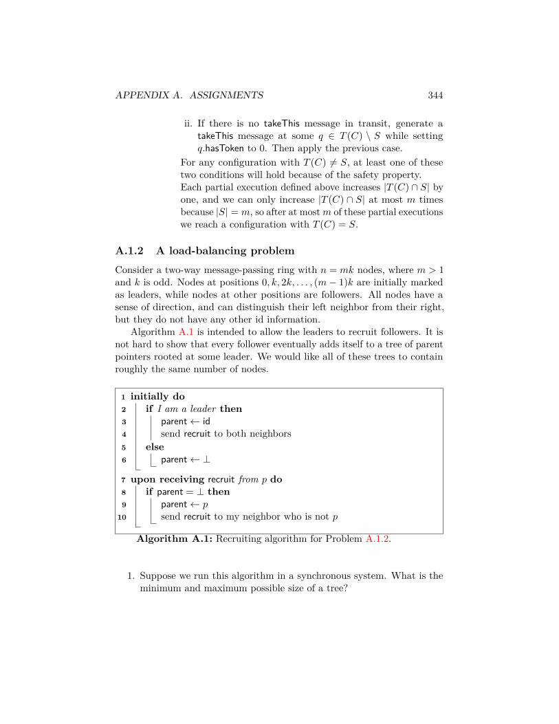
APPENDIX A. ASSIGNMENTS 344

ii. If there is no takeThis message in transit, generate atakeThis message at some q ∈ T (C) \ S while settingq.hasToken to 0. Then apply the previous case.

For any configuration with T (C) 6= S, at least one of thesetwo conditions will hold because of the safety property.Each partial execution defined above increases |T (C) ∩ S| byone, and we can only increase |T (C) ∩ S| at most m timesbecause |S| = m, so after at mostm of these partial executionswe reach a configuration with T (C) = S.

A.1.2 A load-balancing problem

Consider a two-way message-passing ring with n = mk nodes, where m > 1and k is odd. Nodes at positions 0, k, 2k, . . . , (m− 1)k are initially markedas leaders, while nodes at other positions are followers. All nodes have asense of direction, and can distinguish their left neighbor from their right,but they do not have any other id information.

Algorithm A.1 is intended to allow the leaders to recruit followers. It isnot hard to show that every follower eventually adds itself to a tree of parentpointers rooted at some leader. We would like all of these trees to containroughly the same number of nodes.

1 initially do2 if I am a leader then3 parent← id4 send recruit to both neighbors5 else6 parent← ⊥

7 upon receiving recruit from p do8 if parent = ⊥ then9 parent← p

10 send recruit to my neighbor who is not p

Algorithm A.1: Recruiting algorithm for Problem A.1.2.

1. Suppose we run this algorithm in a synchronous system. What is theminimum and maximum possible size of a tree?

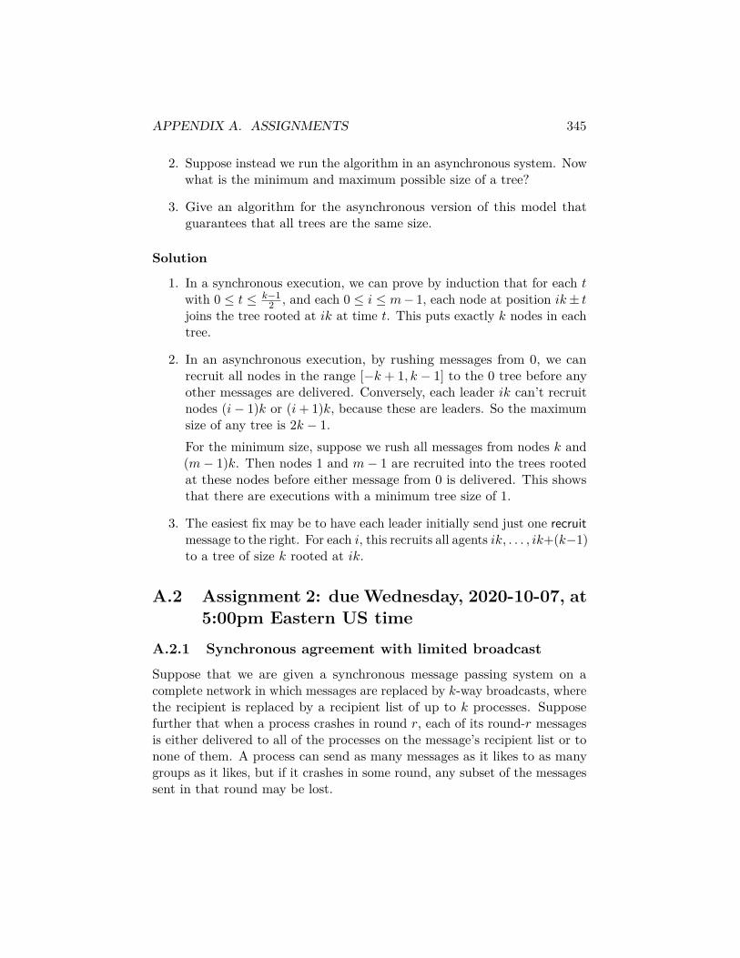
APPENDIX A. ASSIGNMENTS 345

2. Suppose instead we run the algorithm in an asynchronous system. Nowwhat is the minimum and maximum possible size of a tree?

3. Give an algorithm for the asynchronous version of this model thatguarantees that all trees are the same size.

Solution

1. In a synchronous execution, we can prove by induction that for each twith 0 ≤ t ≤ k−1

2 , and each 0 ≤ i ≤ m− 1, each node at position ik± tjoins the tree rooted at ik at time t. This puts exactly k nodes in eachtree.

2. In an asynchronous execution, by rushing messages from 0, we canrecruit all nodes in the range [−k + 1, k − 1] to the 0 tree before anyother messages are delivered. Conversely, each leader ik can’t recruitnodes (i− 1)k or (i+ 1)k, because these are leaders. So the maximumsize of any tree is 2k − 1.For the minimum size, suppose we rush all messages from nodes k and(m− 1)k. Then nodes 1 and m− 1 are recruited into the trees rootedat these nodes before either message from 0 is delivered. This showsthat there are executions with a minimum tree size of 1.

3. The easiest fix may be to have each leader initially send just one recruitmessage to the right. For each i, this recruits all agents ik, . . . , ik+(k−1)to a tree of size k rooted at ik.

A.2 Assignment 2: due Wednesday, 2020-10-07, at5:00pm Eastern US time

A.2.1 Synchronous agreement with limited broadcast

Suppose that we are given a synchronous message passing system on acomplete network in which messages are replaced by k-way broadcasts, wherethe recipient is replaced by a recipient list of up to k processes. Supposefurther that when a process crashes in round r, each of its round-r messagesis either delivered to all of the processes on the message’s recipient list or tonone of them. A process can send as many messages as it likes to as manygroups as it likes, but if it crashes in some round, any subset of the messagessent in that round may be lost.

APPENDIX A. ASSIGNMENTS 346

Show that for it is possible to solve agreement in this model in O(f/k)rounds, assuming n > f .

Solution

We’ll use the flooding algorithm of Dolev and Strong [DS83] (see §9.2), butreplace sending S to all n processes in each round with sending S to all

(nk

)possible recipient lists. As in the original algorithm, we want to prove thatafter some round with few enough failures, all the non-faulty processes havethe same set.

Let Sri be the set stored by process i after r rounds. Suppose there issome round r + 1 in which fewer than k processes fail. Then every recipientlist in round r includes a process that does not fail in round r + 1. Let Lbe the set of processes that successfully deliver a message to at least onerecipient list in round r, and let S = ∪i∈LSri . Then for each value v ∈ S,there is some process that receives v during round r, does not crash in roundr + 1, and so retransmits v to all processes in round r + 1, causing it to beadded to Sr+2

i . On the other hand, for any v 6∈ S, v is not transmitted to anyrecipient list in round r, which means that no non-faulty process i includesv in Sr+1

i . So S ⊆ Sr+2i ⊆ ∪jSr+1

j ⊆ S for all i, and the usual inductionargument shows that Sr′i continues to equal S for all non-faulty i and allr′ ≥ r + 2.

We can have at most bf/kc rounds with ≥ k crashes before we run out,so the latest possible round in which we have fewer than k crashes is isr = bf/kc+ 1, giving agreement after bf/kc+ 2 rounds (since we don’t needto send any messages in round r + 2).

(With some tinkering, it is not too hard to adapt the Dolev-Strong lowerbound to get a bf/kc + 1 lower bound for this model. The main issue isnow we have to crash k processes fully in round r + 1 before we can removeone outgoing broadcast from a process in round r, which means we need tobudget tk failures to break a t-round protocol. The details are otherwisepretty much the same as described in §9.3.)

A.2.2 Asynchronous agreement with limited failures

Algorithm A.2 describes an algorithm for asynchronous agreement with fcrash failures in a fully-connected message-passing network. The idea is tocollect values from n − f other processes in each of m rounds, and thendecide on the smallest value collected.

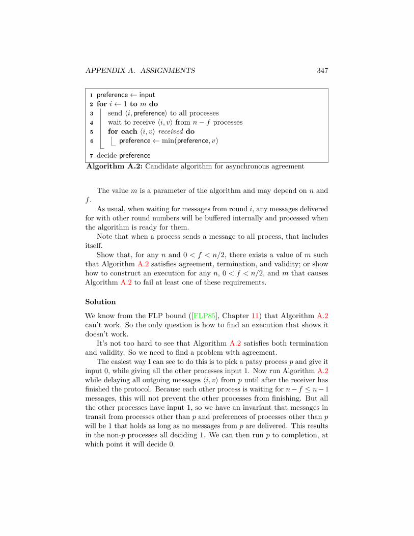
APPENDIX A. ASSIGNMENTS 347

1 preference← input2 for i← 1 to m do3 send 〈i, preference〉 to all processes4 wait to receive 〈i, v〉 from n− f processes5 for each 〈i, v〉 received do6 preference← min(preference, v)

7 decide preferenceAlgorithm A.2: Candidate algorithm for asynchronous agreement

The value m is a parameter of the algorithm and may depend on n andf .

As usual, when waiting for messages from round i, any messages deliveredfor with other round numbers will be buffered internally and processed whenthe algorithm is ready for them.

Note that when a process sends a message to all process, that includesitself.

Show that, for any n and 0 < f < n/2, there exists a value of m suchthat Algorithm A.2 satisfies agreement, termination, and validity; or showhow to construct an execution for any n, 0 < f < n/2, and m that causesAlgorithm A.2 to fail at least one of these requirements.

Solution

We know from the FLP bound ([FLP85], Chapter 11) that Algorithm A.2can’t work. So the only question is how to find an execution that shows itdoesn’t work.

It’s not too hard to see that Algorithm A.2 satisfies both terminationand validity. So we need to find a problem with agreement.

The easiest way I can see to do this is to pick a patsy process p and give itinput 0, while giving all the other processes input 1. Now run Algorithm A.2while delaying all outgoing messages 〈i, v〉 from p until after the receiver hasfinished the protocol. Because each other process is waiting for n− f ≤ n− 1messages, this will not prevent the other processes from finishing. But allthe other processes have input 1, so we have an invariant that messages intransit from processes other than p and preferences of processes other than pwill be 1 that holds as long as no messages from p are delivered. This resultsin the non-p processes all deciding 1. We can then run p to completion, atwhich point it will decide 0.

APPENDIX A. ASSIGNMENTS 348

A.3 Assignment 3: due Wednesday, 2020-10-21, at5:00pm Eastern US time

A.3.1 Too many Byzantine processes

The phase king algorithm (Algorithm 10.2) described in §10.2.2 solves Byzan-tine agreement for f < n/4 processes. For larger values of f , it may fail byviolating one or more of the properties of termination, validity, or agreement.

For this algorithm:

1. How big does f need to be to prevent termination?

2. How big does f need to be to prevent validity?

3. How big does f need to be to prevent agreement?

Assume that the processes know the new bound on f , and any thresholdsin the algorithm that use f are adjusted to correspond to this new bound.

Solution

1. Termination: The algorithm always terminates in f + 1 synchronousrounds, so f doesn’t matter.

2. Validity: To violate validity, we need to convince some non-faultyprocess to decide on the wrong value when all non-faulty processeshave the same input.Suppose all the non-faulty processes have input 0, and we want tointroduce a 1 somewhere. Each process updates its preference ineach round to be either the majority value it sees, if this value hasmultiplicity greater than n/2 + f , or the kingMajority broadcast by thephase king otherwise.If f < n/2, it’s going to be hard to show a process a bogus majority.But a Byzantine phase king gives us more options. Suppose that allthe f Byzantine processes send out 1 in all rounds. Then for f ≥ n/4,the multiplicity of the correct value 0 will be n− f ≤ (3/4)n, while therequired multiplicity to ignore the phase king will be strictly greaterthan n/2 + f ≥ (3/4)n. So at f = n/4, all non-faulty processes adoptthe phase king’s bad value 1. In any subsequent round, we can just runthe algorithm with the Byzantine agents pretending to be non-faultyprocesses with preference 1, and eventually all processes incorrectlydecide 1.

APPENDIX A. ASSIGNMENTS 349

3. Agreement: Now we need to get two non-faulty processes to decidedifferent values. Wait to the last round, and use f = n/4 Byzantineprocesses to prevent the non-faulty processes from seeing a high enoughmultiplicity on any majority value to accept it, and use a Byzantinephase king to transmit different kingMajority values to different non-faulty processes. So again, the algorithm fails at f = n/4.

A.3.2 Committee election

Consider the following committee election problem in an asynchronousmessage-passing system with f < n/2 crash failures. Each process runs acommittee election protocol, at the end of which it receives a value 1 (elected)or 0 (not elected). The requirements of the protocol are:

1. Nonempty committee: If no processes fail, at least one process receives1.

2. No latecomers: In any execution, if some process p finishes the protocolbefore another process q starts the protocol, then q receives 0.

Give an algorithm that solves this problem, and show that it satisfiesthese requirements.

(For the purpose of defining when a process starts or ends the protocol,imagine that it uses explicit invoke and respond events. Your protocol shouldhave the property that all non-faulty processes eventually terminate.)

Solution

The easiest way to do this may be to use ABD (see §16.2). Algorithm A.3has each process read the simulated register, which we assume is initializedto 1, then write a 0 before returning the value it read.

1 Let r be an ABD register initialized to 1.2 procedure elect3 onCommittee← r4 r ← 05 return onCommittee

Algorithm A.3: Committee election using ABD

This satisfies nonempty committee, because the first operation in thelinearization of the register must be a read operation that returns 1. It

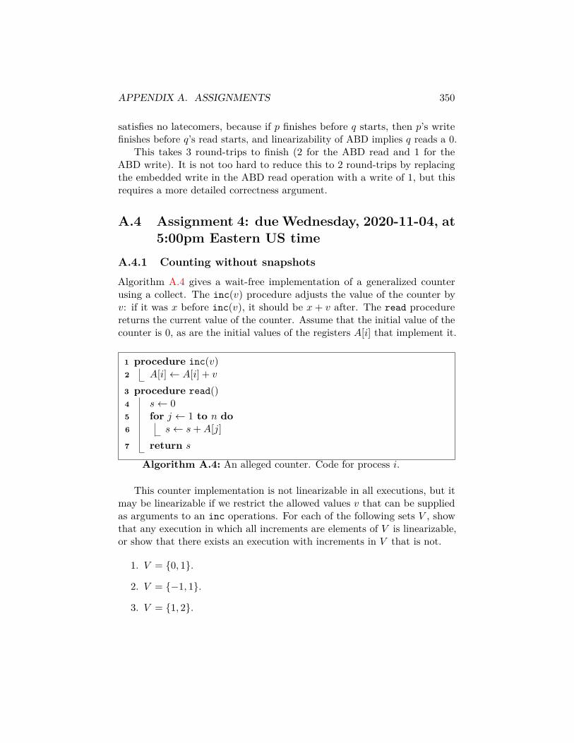
APPENDIX A. ASSIGNMENTS 350

satisfies no latecomers, because if p finishes before q starts, then p’s writefinishes before q’s read starts, and linearizability of ABD implies q reads a 0.

This takes 3 round-trips to finish (2 for the ABD read and 1 for theABD write). It is not too hard to reduce this to 2 round-trips by replacingthe embedded write in the ABD read operation with a write of 1, but thisrequires a more detailed correctness argument.

A.4 Assignment 4: due Wednesday, 2020-11-04, at5:00pm Eastern US time

A.4.1 Counting without snapshots

Algorithm A.4 gives a wait-free implementation of a generalized counterusing a collect. The inc(v) procedure adjusts the value of the counter byv: if it was x before inc(v), it should be x+ v after. The read procedurereturns the current value of the counter. Assume that the initial value of thecounter is 0, as are the initial values of the registers A[i] that implement it.

1 procedure inc(v)2 A[i]← A[i] + v

3 procedure read()4 s← 05 for j ← 1 to n do6 s← s+A[j]7 return s

Algorithm A.4: An alleged counter. Code for process i.

This counter implementation is not linearizable in all executions, but itmay be linearizable if we restrict the allowed values v that can be suppliedas arguments to an inc operations. For each of the following sets V , showthat any execution in which all increments are elements of V is linearizable,or show that there exists an execution with increments in V that is not.

1. V = 0, 1.

2. V = −1, 1.

3. V = 1, 2.

APPENDIX A. ASSIGNMENTS 351

Solution

1. The 0, 1 case is linearizable. Given an execution S of Algorithm A.4,we assign to a linearization point to each inc operation at the stepwhere it writes to A, and assign a linearization point to each readoperation ρ that returns s at the later of the first step that leaves∑j A[j] = s or the first step of ρ. Since this may assign the same

linearization point to some write operation π and one or more readoperations ρ1, . . . , ρk, when this occurs, we order the write before thereads and the reads arbitrarily.Observe that:

(a) The value of each A[j] individually is non-decreasing over time,and increases by at most one at each step.

(b) The same holds for∑nj=1A[j].

These are easily shown by induction on the steps of the execution, sinceeach inc operation only changes at most one A[j] and only changes itby increasing it by 1.The first condition implies that the value vj of A[j] used by a particularread operation ρ lies somewhere between the minimum and maximumvalues of A[j] during the operation’s interval, which implies the sameabout the total

∑j A[j]. In particular, if ρ returns s the value of∑

j A[j] is no greater than s, and it reaches s no later than the end ofρ.Because

∑j A[j] increases by at most one per step, this means that

either∑j A[j] = s at the first step of ρ, or

∑j A[j] = s at some step

within the execution interval of ρ. In either case, ρ is assigned anexecution point within its interval that follows exactly s non-trivialincrements. This means that the return values of all read operationsare consistent with a sequential generalized counter execution, andbecause both read and inc operations are ordered consistently withthe execution ordering in S, we have a linearization of S.

2. For increments in −1, 1, there are executions of Algorithm A.4 thatare not linearizable. We will construct a specific bad execution forn = 3. Let p1 perform inc(1) and p2 perform inc(2), where p1 finishesits operation before p2 starts. Because the inc(1) must be linearizedbefore the inc(−1), the values of the counter in any linearization willbe 0, 1, 0 in this order.

APPENDIX A. ASSIGNMENTS 352

Now add a read operation by p3 that is concurrent with both incoperations. Suppose that in the execution, the follow operations areperformed on the registers A[1] through A[3]:

(a) p3 reads 0 from A[1].(b) p1 writes 1 to A[1].(c) p2 writes −1 to A[2].(d) p3 reads −1 from A[2].(e) p3 reads 0 from A[3].

Now p3 returns −1. There is no point in the sequential execution atwhich this is the correct return value, so there is no linearization ofthis execution.

3. For increments in 1, 2, essentially the same counterexample works.Here we let p1 do inc(1) and p2 do inc(2), while p3 again does aconcurrent read. The bad execution is:

(a) p3 reads 0 from A[1].(b) p1 writes 1 to A[1].(c) p2 writes 2 to A[2].(d) p3 reads 2 from A[2].(e) p3 reads 0 from A[3].

Now p3 returns 2, but in any linearization of the two write operations,the values in the counter are 0, 1, 3.

A.4.2 Rock-paper-scissors

Define a rock-paper-scissors object as having three states 0 (rock), 1(paper), and 2 (scissors), with a read operation that returns the currentstate and a play(v) operation for v ∈ 0, 1, 2 that changes the state from sto v if v = (s+ 1) (mod 3) and has no effect otherwise.

Prove or disprove: There exists a deterministic wait-free linearizableimplementation of a rock-paper-scissors object from atomic registers.

APPENDIX A. ASSIGNMENTS 353

Solution

Proof: We will show how to implement a rock-paper-scissors object usingan unbounded max register, which can be built from atomic registers usingsnapshots. The idea is to store a value v such that v mod 3 gives the valueof the rock-paper-scissors object. Pseudocode for both operations is given inAlgorithm A.5.

1 Let m be a shared max register.2 procedure play(v)3 s← m4 if v = ((s+ 1) mod 3) then5 m← s+ 1

6 procedure read()7 return (m mod 3)

Algorithm A.5: Implementation of a rock-paper-scissors object

Linearize each play operation that does not write m at the step at whichit reads m.

Linearize each play operation that writes s + 1 to m at the first stepat which m ≥ s+ 1. If this produces ties, break first in order of increasings+ 1 and then arbitrarily. Since each such operation has m ≤ s when theoperation starts and m ≥ s+ 1 when it finishes, these linearization points fitwithin the intervals of their operations.

Linearize each read() operation at the step where it reads m.Since each of these linearization points is within the corresponding oper-

ation’s interval, this preserves the observed execution ordering.Observe that the play operations that write are linearized in order of

increasing values written, and there are no gaps in this sequence becauseno process writes s+ 1 without first seeing s. (This actually shows there isno to break ties by value.) So the sequence of values in the max register,taken mod 3, iterates through the values 0, 1, 2, 0, . . . in sequence, with eachvalue equal mod 3 to some argument to a play operation. So we can takethese values mod 3 as the actual value of the register for the purposes ofread operations, meaning the read operations all return correct values. Theplay operations that don’t write are linearized at a point where they wouldhave no effect on the state of the rock-paper-scissors object, which is alsoconsistent with the sequential specification.

It follows that Algorithm A.5 is a linearizable implementation of a rock-

APPENDIX A. ASSIGNMENTS 354

paper-scissors object from max registers. It is also wait-free, since eachoperation is implemented using a constant number of max-register operations.By implementing max registers using snapshots, we get a wait-free linearizableimplementation from atomic registers.

A.5 Assignment 5: due Wednesday, 2020-11-18, at5:00pm Eastern US time

A.5.1 Randomized consensus with one max register

Prove or disprove: A single max register, with no other objects, is sufficientto solve randomized wait-free binary consensus for two processes against anoblivious adversary.

Solution

We’ll disprove it.Let p0 and p1 be the two processes. The idea is to consider, for each

i ∈ 0, 1 some nonzero-probability solo terminating execution ξi of pi withinput i, then show that ξ0 and ξ1 can be interleaved to form a two-processexecution ξ that is indistinguishable by each pi from ξi.

The oblivious adversary will simply choose to schedule the processes forξ. Since the processes flip a finite number of coins in this execution, thereis a nonzero chance that the adversary gets lucky and they flip their coinsexactly the right way.

Fix ξ0 and ξ1 as above. Partition each ξi as αiβi1βi2 . . . βiki where αicontains only read operations and each βij starts with a write operation of avalue vij strictly larger than any previous write operation.

Let ξ = α0α1βi1j1βi2j2 . . . βikjk where k = k0 + k1 and the blocks βi`j` arethe blocks β0j and β1j sorted in order of non-decreasing vij . Then eachblock βi`j` in ξ starts with a write of a value no smaller than the previousvalue in the max register, causing each read operation within the block toreturn the value of this write, just as in the solo execution ξi` . Assumingboth processes flip their coins as in the solo executions, they both performthe same operations and return the same values. These values will eitherviolate agreement in ξ or validity in at least one of ξ0 or ξ1.

APPENDIX A. ASSIGNMENTS 355

A.5.2 A plurality object

Consider a shared-memory object with operations vote(v) and winner(),where winner() returns the value v that appeared in the largest number ofprevious vote operations, or ⊥ if there is no such unique v. For example, ina sequential execution with votes a, b, b, c, c, c, a, a, a, the value returned by awinner operation following each vote will be a,⊥, b, b,⊥, c, c,⊥, a.

Pick one of these statements, and show that it is true:

1. There is a deterministic wait-free linearizable implementation of thisobject for n processes that uses o(n) registers.

2. There is such an implementation that uses O(n) registers, but not o(n)registers.

3. There is no such implementation using O(n) registers.

Solution

Case (2) holds.To implement the object, use a snapshot array to hold the total votes

from each process, and have the winner operation take a snapshot, add upall the votes and return the correct result. This can be done using n registers.

To show that it can’t be done with o(n) registers, use the JTT bound (seeChapter 20). We need to argue that the object is perturbable. Let ΛΣπ bean execution that needs to be perturbed, and let m be the maximum numberof vote(v) operations that start in Λ for any value v. Then a sequence γ ofm+1 votes for some v′ that does not appear in Λ will leave the object with v′as the plurality value, no matter how the remaining operations are linearized.Since v′ did not previously appear in Λ, this gives a different return valuefor π in ΛγΣπ from ΛΣπ as required. The JTT bound now implies that anyimplementation of the object requires at least n− 1 registers.

A.6 Presentation (for students taking CPSC 565):due Tuesday, 2020-12-01, or Thursday, 2020-12-03, in class; paper selection due Friday,2020-11-20.

Students taking CPSC 565, the graduate version of the class, are expected togive a 10-minute presentation on a recent paper in the theory of distributedcomputing.

APPENDIX A. ASSIGNMENTS 356

The choice of paper to present should be made in consultation with theinstructor. To a first approximation, any paper from PODC, DISC, or asimilar conference in the last two or three years (that is not otherwise coveredin class) should work.

Please use the form at https://forms.gle/qafxrqiCPvYbQjQP7 to sub-mit your proposed paper and preferred presentation time.

To get you started, the program for PODC 2020 can be found at https://www.podc.org/podc2020/program/. The web page for DISC 2020 can befound at http://www.disc-conference.org/wp/disc2020/. Both includelinks to papers published in the conference and to videos of conferencepresentations.

Because of the limited presentation time, you are not required to getinto all of the technical details of the paper, but your presentation shouldinclude:2

1. Title, authors, and date and venue of publication of the paper.

2. A high-level description of a central result. Unlike a talk for a generalaudience, you can assume that your listeners know at least everythingthat we’ve talked about so far in the class.

3. A description of where this result fits into the literature (e.g., solvesan open problem previously proposed in [...], improves on the previousbest running time for an algorithm from [...], gives a lower bound orimpossibility result for a problem previously proposed by [...], opensup a new area of research for studying [...]), and why it is interestingand/or hard.

4. A description (also possibly high-level) of the main technical mecha-nism(s) used to get the result.

You do not have to prepare slides for your presentation if you wouldprefer to use the whiteboard feature in Zoom, but you should make sureto practice it in advance to make sure it fits in the allocated time. Theinstructor will be happy to offer feedback on draft versions if available farenough before the actual presentation date.

Relevant dates:2Literary theorists will recognize this as a three-act structure (preceded by a title card):

introduce the main character, make their life difficult, then resolve their problems in timefor the final curtain. This is not the only way to organize a talk, but if done right it hasthe advantage of keeping the audience awake.

APPENDIX A. ASSIGNMENTS 357

2020-11-20 Paper selection due.

2020-11-27 Last date to send draft slides or arrange for a practice presen-tation with the instructor if you want guaranteed feedback.

2020-12-01 and 2020-12-03 Presentations, during the usual class time.

Appendix B

Sample assignments fromSpring 2019

B.1 Assignment 1: due Wednesday, 2019-02-13, at5:00pm

B.1.1 A message-passing bureaucracy

Alice and Bob are communicating with each other by alternately exchangingmessages. But Bob finds Alice’s messages alarming, and whenever he respondsto Alice, he also forwards a copy of Alice’s message to his good friend Charlie1, a secret policeman. Charlie 1 reports to Charlie 2, but following the rulethat “once is happenstance, twice is coincidence, the third time it’s enemyaction,” [Fle59] Charlie 1 only sends a report to Charlie 2 after receivingthree messages from Bob. Similarly, Charlie 2 only sends a message to hissupervisor Charlie 3 after receiving three messages from Charlie 2, and soon up until the ultimate boss Charlie n. Pseudocode for each participant isgiven in Algorithm B.1.

Assuming we are in a standard asynchronous message-passing system,that Alice sends her first message at time 0, and that the protocol finishesas soon as Charlie n receives a message, what is the worst-case time andmessage complexity of this protocol as a function of n?

Solution

Time complexity Observe that Alice sends at least k messages by time2k − 2. This is easily shown by induction on k, because Alice sends at least1 message by time 0, and if Alice has sent at least k − 1 message by time

358

APPENDIX B. SAMPLE ASSIGNMENTS FROM SPRING 2019 359

1 Alice:2 initially do3 send message to Bob4 upon receiving message from Bob do5 send message to Bob6 Bob:7 upon receiving message from Alice do8 send message to Alice9 send message to Charlie 1

10 Charlie i, for i < n:11 initially do12 c← 013 upon receiving message from Bob or Charlie i− 1 do14 c← c+ 115 if c = 3 then16 c← 017 send message to Charlie i+ 1

Algorithm B.1: Reporting Alice’s alarming messages

APPENDIX B. SAMPLE ASSIGNMENTS FROM SPRING 2019 360

2k − 4, the last of these is received by Bob no later than time 2k − 3, andBob’s response is received by Alice no later than time 2k − 2.

Because each message from Alice prompts a message from Bob at mostone time unit later, this implies that Bob sends at least k messages by time2k − 1.

Write T0(k) = 2k − 1 for the maximum time for Bob to send k messages.Write Ti(k) for the maximum time for Charlie i to send k messages, foreach 0 < i < n. In order for Charlie i to send k messages, it must receive3k messages from Bob or Charlie i− 1 as appropriate. These messages aresent no later than Ti−1(3k), and the last of them is received no later thanTi−1(3k) + 1. So we have the recurrence

Ti(k) = Ti−1(3k) + 1T0(k) = 2k − 1

with the exact solution

Ti(k) = (2 · 3i · k − 1) + k.

For i = n− 1 and k = 1, this is 2 · 3n−1− 1 +n− 1 = 2 · 3n−1 +n = O(3n).We can get the exact time to finish by adding one more unit to account forthe delay in delivering the message from Charlie n− 1 to Charlie n. Thisgives 2 · 3n−1 + n+ 1 time exactly in the worst case, or O(3n) if we want anasymptotic bound.

Message complexity Message complexity is easier: there is no bound onthe number of messages that may be sent before Charlie n receives his firstmessage. This is because in an asynchronous system, Alice and Bob can sendan unbounded (though finite) number of messages to each other even beforeBob’s first message to Charlie 0 is delivered, without violating fairness.

B.1.2 Algorithms on rings

In Chapter 5, we saw several leader election algorithms for rings. But nobodybuilds rings. However, it may be that an algorithm for a ring can be adaptedto other network structures.

1. Suppose you have a network in the form of a d-dimensional hypercubeQd. This means we have n = 2d nodes, where each node is labeled bya d-bit coordinate vector, and two nodes are adjacent if their vectors

APPENDIX B. SAMPLE ASSIGNMENTS FROM SPRING 2019 361

differ in exactly one coordinate. We also assume that each node knowsits own coordinate vector and those of its neighbors.Show that any algorithm for an asynchronous ring can be adapted toan asynchronous d-dimensional hypercube with no increase in its timeor message complexity.

2. What difficulties arise if we try to generalize this to an arbitrary graphG?

Solution

1. The idea is to embed the ring in the hypercube, so that each node isgiven a clockwise and counterclockwise neighbors, and any time the ringalgorithm asks to send a message clockwise or counterclockwise, we sendto the appropriate neighbor in the hypercube. We can then argue thatfor any execution of the hypercube algorithm there is a correspondingexecution of the ring algorithm and vice versa; this implies that theworst-case time and message-complexity in the hypercube is the sameas in the ring.It remains only to construct an embedding. For d = 0, d = 1, and d = 2,the ring and hypercube are the same graph, so it’s easy. For largerd, split the hypercube into two subcubes Qd−1, consisting of nodeswith coordinate vectors of the form 0x and 1x. Use the previouslyconstructed embedding for d − 1 to embed a ring on each subcube,using the same embedding for both. Pick a pair of matching edges(0x, 0y) and (1x, 1y) and remove them, replacing them with (0x, 1x)and (0y, 1y). We have now constructed an undirected Hamiltoniancycle on Qd. Orient the edges to get a directed cycle, and we’re done.

2. There are a several problems that may come up:

(a) Maybe G is not Hamiltonian.(b) Even if G is Hamiltonian, finding an Hamiltonian cycle in an

arbitrary graph is NP-hard. This could be trouble for a practicalalgorithm.

(c) Even if we can find a Hamiltonian cycle for G (maybe because Gis a nice graph of some kind, or maybe by taking advantage ofthe unbounded computational power of processes assumed in thestandard message-passing model), the processes don’t necessarilyknow what G looks like at the start. So they would need some

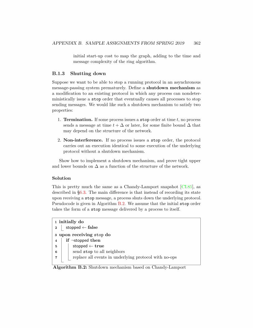
APPENDIX B. SAMPLE ASSIGNMENTS FROM SPRING 2019 362

initial start-up cost to map the graph, adding to the time andmessage complexity of the ring algorithm.

B.1.3 Shutting down

Suppose we want to be able to stop a running protocol in an asynchronousmessage-passing system prematurely. Define a shutdown mechanism asa modification to an existing protocol in which any process can nondeter-ministically issue a stop order that eventually causes all processes to stopsending messages. We would like such a shutdown mechanism to satisfy twoproperties:

1. Termination. If some process issues a stop order at time t, no processsends a message at time t+ ∆ or later, for some finite bound ∆ thatmay depend on the structure of the network.

2. Non-interference. If no process issues a stop order, the protocolcarries out an execution identical to some execution of the underlyingprotocol without a shutdown mechanism.

Show how to implement a shutdown mechanism, and prove tight upperand lower bounds on ∆ as a function of the structure of the network.

Solution

This is pretty much the same as a Chandy-Lamport snapshot [CL85], asdescribed in §6.3. The main difference is that instead of recording its stateupon receiving a stop message, a process shuts down the underlying protocol.Pseudocode is given in Algorithm B.2. We assume that the initial stop ordertakes the form of a stop message delivered by a process to itself.

1 initially do2 stopped← false3 upon receiving stop do4 if ¬stopped then5 stopped← true6 send stop to all neighbors7 replace all events in underlying protocol with no-ops

Algorithm B.2: Shutdown mechanism based on Chandy-Lamport

APPENDIX B. SAMPLE ASSIGNMENTS FROM SPRING 2019 363

An easy induction argument shows that if p receives a stop message attime t, then any process q at distance d from p receives a stop message nolater than time t+ d. It may be that q sends stop messages in responds tothis stop message, but these are the last messages q ever sends. It followsthat no process sends a message later than time t + D, where D is thediameter of the graph. This gives an upper bound on ∆.

For the lower bound, we can apply an indistinguishability argument. Letp and q be processes at distance D from each other, and suppose that theunderlying protocol involves processes sending messages to their neighbors atevery opportunity. Consider two synchronous executions: X, an execution inwhich no stop order is ever issued, and Xt, an execution in which p deliversa stop message to itself at time t.

We can show by induction on d that any process r at distance d from pcarries out the same steps in both X and Xt up until time t+d−1. The basecase is when d = 0, and we are simply restating that p runs the underlyingprotocol before time t. For the induction step, we observe for any timet′ < t+ d− 1, any message sent to r from some neighbor s was sent at timet′ − 1 < t+ d− 2, and since d(p, s) ≥ d− 1, the induction hypothesis givesthat s sends the same messages at t′ − 1 in both X and Xt.

It follows that q sends the same message in X and Xt at time t+D − 1.If it sends a message, then we have ∆ > D− 1. If it does not send a message,then the mechanism violates the non-interference condition. So any correctshutdown mechanism requires exactly ∆ = D time to finish in the worstcase.

B.2 Assignment 2: due Wednesday, 2019-03-06, at5:00pm

B.2.1 A non-failure detector

Consider the following vaguely monarchist leader election mechanism for anasynchronous message-passing system with crash failures. Each process hasaccess to an oracle that starts with the value 0 and may increase over time.The oracle guarantees:

1. No two processes ever see the same nonzero value.

2. Eventually some non-faulty process is given a fixed value that is largerthan the values for all other processes for the rest of the execution.

APPENDIX B. SAMPLE ASSIGNMENTS FROM SPRING 2019 364

As a function of the number of processes n, what is the largest number ofcrash failures f for which it is possible to solve consensus using this oracle?

Solution

We need f < n/2.To show that f < n/2 is sufficient, observe that we can use the oracle to

construct an eventually strong (♦S) failure detector.Recall that ♦S has the property that there is some non-faulty process

that is eventually never suspected, and every fault process is eventuallypermanently suspected. Have each process broadcast the current value of itsleader oracle whenever it increases; when a process p receives i from someprocess q, it stops suspecting q if i is greater than any value p has previouslyseen, and starts suspecting all other processes. The guarantee that eventuallysome non-faulty q gets a maximum value that never changes ensures thateventually q is never suspected, and all other processes (including faultyprocesses) are suspected. We can now use Algorithm 13.2 to solve consensus.

To show that f < n/2 is necessary, apply a partition argument. Inexecution Ξ0, processes n/2 + 1 through n crash, and processes 1 throughn/2 run with input 0 and with the oracle assigning value 1 to process 1 (andno others). In execution Ξ1, processes 1 through n/2 crashes, and processesn/2 + 1 through n run with input 1 and with the oracle assigning value 2to process n (and no others). In each of these executions, termination andvalidity require that eventually the processes all decide on their respectiveinput values 0 and 1.

Now construct an execution Ξ2, in which both groups of processes runas in Ξ0 and Ξ1, but no messages are exchanged between the groups untilafter both have decided (which must occur after a finite prefix because thisexecution is indistinguishable to the processes from Ξ0 or Ξ1). We nowviolate agreement.

B.2.2 Ordered partial broadcast

Define ordered partial broadcast as a protocol that allows any processto broadcast a message, with the guarantees that, for messages sent throughthe broadcast mechanism:

1. Any message sent by a non-faulty process is received by at least oneprocess;

2. Any message that is received by at least one process is received by atleast k processes; and

APPENDIX B. SAMPLE ASSIGNMENTS FROM SPRING 2019 365

3. If two processes p and q both receive messages m1 and m2 from theprotocol, then either p and q both receive m1 before m2, or they bothreceive m2 before m1.

Give an implementation of ordered partial broadcast with k = 3n/4 thatworks for sufficiently large n in a fully-connected asynchronous message-passing system with up to f = n/6 crash failures, or show that no suchimplementation is possible.

Solution

No such implementation is possible. The proof is by showing that if somesuch implementation could work, we could solve asynchronous consensus with1 crash failure, contradicting the Fischer-Lynch-Patterson bound [FLP85](see Chapter 11).

An implementation of consensus based on totally-ordered partial broad-cast for k = 3n/4 is given in Algorithm B.3. In fact, k = 3n/4 is overkillwhen f = 1; k > n/2 + f is enough.

1 first← ⊥2 for i← 1ton do3 count[i]← 04 value[i]← ⊥5 broadcast 〈i, input〉6 upon receiving 〈j, v〉 do7 if first = ⊥ then8 first← 〈j, v〉9 send received(〈j, v〉) to all processes

10 upon receiving received(〈j, v〉) do11 count[j]← count[j] + 112 value[j]← v13 if count[j] = k − f then14 decide value[j]

Algorithm B.3: Consensus from totally-ordered partial broadcast.Code for process i.

The idea of the algorithm is to use the broadcast mechanism to chose adecision value, by looking at which value is delivered first. Since not everyprocess will see the same value delivered first, this requires a second round

APPENDIX B. SAMPLE ASSIGNMENTS FROM SPRING 2019 366

of communication in which processes retransmit their first incoming message.The following lemma shows that this is enough to get agreement:

Lemma B.2.1. In any execution of Algorithm B.3 with k > n/2 + f . thereis a unique pair 〈j, v〉 such that at least k − f non-faulty processes resendreceived(〈j, v〉).

Proof. Because all processes that receive messages m1 and m2 through thebroadcast mechanism receive them in the same order, we can define a partialorder on messages by letting m1 < m2 if any process receives m1 before m2.

There are only finitely many messages, so there is at least one pair 〈j, v〉that is minimal in this partial order. This message is received by at least kprocesses, of which at least k − f are non-faulty. Each such process receives〈j, v〉 before any other broadcast messages, so it sets first to 〈j, v〉 and resendsreceived(〈j, v〉).

To show that 〈j, v〉 is unique, observe that k − f > n/2 implies that ifthere is some other pair 〈j′, v′〉 that is resent by k − f non-faulty processes,then there is some process that resends both 〈j, v〉 and 〈j′, v′〉. But eachprocess resends at most one pair.

Lemma B.2.1 immediately gives agreement, because a process only decideson a value v after receiving received(〈j, v〉) from k − f processes, and onlyone such pair is sent by so many. Termination follows from the existence ofsuch a pair: eventually every non-faulty process receives 〈j, v〉 from k − fprocesses. Validity is immediate from the fact that v is j’s input.

It follows that Algorithm B.3 solves consensus whenever k > n/2 + f ,which includes the case k = 3n/4 and f = n/6. If an implementationof ordered partial broadcast with these parameters exists in the standardmessage-passing model, this would give a protocol for asynchronous consensuswith f = n/6 ≥ 1 when n ≥ 6. This contradicts FLP, showing that such animplementation is impossible.

B.2.3 Mutual exclusion using a counter

Algorithm B.4 gives a modified version of Peterson’s two-process mutualexclusion algorithm (§17.4.1) that replaces the present bits with an atomiccounter count. This object supports read, increment, and decrement opera-tions, where increment and decrement increase and decrease the value in thecounter by one, respectively. Unlike the present array, count doesn’t dependon the number of processes n. So in principle this algorithm might work forarbitrary n.

APPENDIX B. SAMPLE ASSIGNMENTS FROM SPRING 2019 367

shared data:1 waiting, atomic register, initially arbitrary2 count, atomic counter, initially 03 Code for process i:4 while true do

// trying5 increment count6 waiting← i7 while true do8 if count = 1 then9 break

10 if waiting = i+ 1 (mod n) then11 break

// critical12 (do critical section stuff)

// exiting13 decrement count

// remainder14 (do remainder stuff)

Algorithm B.4: Peterson’s mutual exclusion algorithm using acounter

APPENDIX B. SAMPLE ASSIGNMENTS FROM SPRING 2019 368

Show that Algorithm B.4 provides starvation-free mutual exclusion fortwo processes, but not for three processes.

Solution

The proof that this works for two processes is essentially the same as in theoriginal algorithm. The easiest way to see this is to observe that processpi sees count = 1 in Line 8 under exactly the same circumstances as it seespresent[¬i] = 0 in Line 8 in the original algorithm; and similarly with twoprocesses waiting is always set to the same value as waiting in the originalalgorithm. So we can map any execution of Algorithm B.4 for two processesto an execution of Algorithm 17.4, and all of the properties of the originalalgorithm carry over to the modified version.

To show that the algorithm doesn’t work for three processes, we constructan explicit bad execution:

1. p0 increments count

2. p1 increments count

3. p2 increments count

4. p0 writes 0 to waiting

5. p1 writes 1 to waiting

6. p2 writes 2 to waiting

7. p0 reads 3 from count

8. p1 reads 3 from count

9. p2 reads 3 from count

10. p1 reads 2 from waiting and enters the critical section.

11. p1 leaves the critical section and decrements count.

At this point we have count = 2 and waiting = 2, with both p0 and p2 atthe start of the loop to check these variables. Suppose that p1 doesn’t comeback. Because neither p0 nor p2 changes count or waiting, both variablesremain at 2 forever. But then neither p0 nor p2 enters the critical section,because count is never 1 and waiting is never equal to 0 + 1 or 2 + 1 (mod 3).

APPENDIX B. SAMPLE ASSIGNMENTS FROM SPRING 2019 369

B.3 Assignment 3: due Wednesday, 2019-04-17, at5:00pm

B.3.1 Zero, one, many

Consider a counter supporting inc and read operations that is capped at 2.This means that after the first two calls to inc, any further calls to inc haveno effect: a read operation will return 0 if it follows no calls to inc, 1 if itfollows exactly one call to inc, and 2 if it follows two or more calls to inc.

There is a straightforward implementation of this object using snapshot.This requires O(n) space and O(n) steps per operation in the worst case.

Is it possible to do better? That is, can one give a deterministic, wait-free,linearizable implementation of a 2-bounded counter from atomic registersthat uses o(n) space and o(n) steps per operation in the worst case?

Solution

One possible implementation is given in Algorithm B.5. This requires O(1)space and O(1) steps per call to inc or read.

1 procedure inc2 if c[1] = 1 then

// somebody already did inc3 c[2]← 14 else5 c[1]← 1

// maybe somebody else is doing inc6 if splitter returns right or down then7 c[2]← 1

8 procedure read9 if c[2] = 1 then

10 return 211 else if c[1] = 1 do12 return 113 else14 return 0

Algorithm B.5: A 2-bounded counter

APPENDIX B. SAMPLE ASSIGNMENTS FROM SPRING 2019 370

The implementation uses two registers c[1] and c[2] to represent the valueof the counter. Two additional registers implement a splitter object as inAlgorithm 17.5.1

Claim: For any two calls to inc, at least one sets c[2] to 1. Proof: Supposeotherwise. Then both calls are by different processes p and q (or else thesecond call would see c[1] = 1) and both execute the splitter. Since a splitterreturns stop to at most one process, one of the two processes gets right ordown, and sets c[2].

It is also straightforward to show that a single inc running alone will setc[1] but not c[2], since in this case the splitter will return stop.

Now we need to argue linearizability. We will do so by assigning lineariza-tion points to each operation.

If some inc does not set c[2], assign it the step at which it sets c[1].Assign each other inc the step at which it first sets c[2].

If every inc sets c[2], assign the first inc to set c[1] the step at which itdoes so, and assign all others the first point during its execution interval atwhich c[2] is nonzero.

For a read operation that returns 2, assign the step at which it reads c[2].For a read operation that returns 1, assign the first point in the executioninterval after it reads c[2] at which c[1] = 1. For a read operation thatreturns 0, assign the step at which it reads c[0].

This will assign the same linearization point to some operations; in thiscase, put incs before reads and otherwise break ties arbitrarily.

These choices create a linearization which consists of (a) a sequence ofread operations that return 0, all of which are assigned linearization pointsbefore the first step at which c[1] = 1; (b) the first inc operation thatsets c[1]; (c) a sequence of read operations that return 1, all of which arelinearized after c[1] = 1 but before c[2] = 1; (c) some inc that is eitherthe first to set c[2] or spans the step that sets c[2]; and (d) additional incoperations together with read operations that all return 2. Since each readreturns the minimum of 2 and the number of incs that precede it, this is acorrect linearization.

B.3.2 A very slow counter

Consider a slow counter object with operations inc and read, where thevalue v of a counter starts at 0 and increases by 1 as the result of each call

1It may be possible shave off a register by breaking the splitter abstraction and usingthe race or door register in place of c[1], but I haven’t worked out the linearizability forthis case.

APPENDIX B. SAMPLE ASSIGNMENTS FROM SPRING 2019 371

to inc, but read returns log∗ v instead of v.Suppose we want a deterministic, wait-free, linearizable implementation

of a slow counter as defined above from atomic registers. Give tight boundson the worst-case step complexity of operations on such an implementation.

Solution

The worst-case step complexity of an operation is Θ(n).For the upper bound, implement a counter on top of snapshots (or just

collect), and have read compute log∗ of whatever value is read.For the lower bound, observe that a slow counter has the perturbability

property needed for the JTT proof. Given an execution of the form ΛkΣkπas described in Chapter 20, we can always insert some sequence of incoperations between Λk and Σk that will change the return value of π. Thenumber of incs needed will be the number needed to raise log∗ v, plus anextra n to overcome the possibility of pending incs in Σk being linearizedbefore or after π. Since this object is perturbable, and the atomic registerswe are implementing it from are historyless, JTT applies and gives an Ω(n)lower bound on the cost of read in the worst case.

B.3.3 Double-entry bookkeeping

Consider an object that implements an unbounded collection of accountsA1, A2, . . . , each of which holds an integer value, and that provides threeoperations:

• The operation read(i) returns the current value of Ai.

• The operation transfer(i, j, n) moves n units from Ai to Aj ; if A′i andA′j are the new values, then A′i = Ai − n and A′j = Aj + n.

• The operation close(i, j) sets Ai to zero and adds the previous valueto Aj . It is equivalent to atomically executing transfer(i, j, read(i)).

1. What is the consensus number of this object?

2. What is the consensus number of a restricted version of this objectthat provides only the read and transfer operations?

APPENDIX B. SAMPLE ASSIGNMENTS FROM SPRING 2019 372

Solution

1. The consensus number of the object is infinite. Initialize A0 to 1 andthe remaining Ai to 0. We can solve id consensus by having processi (where i > 0 execute close(0, i) and then applying read to scan allthe Aj values for itself and other processes. Whichever process getsthe 1 wins.

2. The consensus number without close is 1. Proof: Observe thattransfer operations commute.

B.4 Presentation (for students taking CPSC 565):due Monday, 2019-04-22, or Wednesday, 2019-04-24, in class

Students taking CPSC 565, the graduate version of the class, are expected togive a 10-minute presentation on a recent paper in the theory of distributedcomputing.

The choice of paper to present should be made in consultation with theinstructor. To a first approximation, any paper from PODC, DISC, or asimilar conference in the last two or three years (that is not otherwise coveredin class) should work.

To get you started, the 2018 PODC proceedings can be found at https://dl.acm.org/citation.cfm?id=3212734&picked=prox, and the 2018 DISCproceedings can be found at http://drops.dagstuhl.de/opus/portals/lipics/index.php?semnr=16090.

Because of the limited presentation time, you are not required to getinto all of the technical details of the paper, but your presentation shouldinclude:2

1. Title, authors, and date and venue of publication of the paper.

2. A high-level description of a central result. Unlike a talk for a generalaudience, you can assume that your listeners know at least everythingthat we’ve talked about so far in the class.

2Literary theorists will recognize this as a three-act structure (preceded by a title card):introduce the main character, make their life difficult, then resolve their problems in timefor the final curtain. This is not the only way to organize a talk, but if done right it hasthe advantage of keeping the audience awake.

APPENDIX B. SAMPLE ASSIGNMENTS FROM SPRING 2019 373

3. A description of where this result fits into the literature (e.g., solvesan open problem previously proposed in [...], improves on the previousbest running time for an algorithm from [...], gives a lower bound orimpossibility result for a problem previously proposed by [...], opensup a new area of research for studying [...]), and why it is interestingand/or hard.

4. A description (also possibly high-level) of the main technical mecha-nism(s) used to get the result.

You do not have to prepare slides for your presentation if you wouldprefer to use the blackboard, but you should make sure to practice it inadvance to make sure it fits in the allocated time. The instructor will behappy to offer feedback on draft versions if available far enough before theactual presentation date.

Relevant dates:

2019-04-10 Paper selection due.

2019-04-17 Last date to send draft slides or arrange for a practice presen-tation with the instructor if you want guaranteed feedback.

2019-04-22 and 2019-04-24 Presentations, during the usual class time.

B.5 CS465/CS565 Final Exam, May 7th, 2019Write your answers in the blue book(s). Justify your answers. Work alone.Do not use any notes or books.

There are four problems on this exam, each worth 20 points, for a totalof 80 points. You have approximately three hours to complete this exam.

B.5.1 A roster (20 points)

A roster object has operations announce and read, where read returns alist of the identities of all processes that have previously called announce atleast once.

Suppose you want a wait-free, linearizable implementation of this objectfrom multiwriter atomic registers. As a function of the number of processesn, give the best upper and lower bound you can on the number of registersyou will need.

You may assume that the set of process identities is fixed for each n andthat each process knows its own identity.

APPENDIX B. SAMPLE ASSIGNMENTS FROM SPRING 2019 374

Solution

You will need exactly n registers (Θ(n) is also an acceptable answer).For the upper bound, have each process write its id to its own register,

and use a double-collect snapshot to read all of them. This uses exactly nregisters. The double-collect snapshot is wait-free because after each processhas called announce once, the contents of the registers never change, so readfinishes after O(n) collects or O(n2) register reads. It’s linearizable becausedouble-collect snapshot returns the exact contents of the registers at somepoint during its execution.3

For the lower bound, use a covering argument.4Have the processes p1, . . . , pn run announce in order, stopping each

process when it covers a new register. This will give sequence of partialexecutions Ξi where at the end of Ξi, there is a set of i registers r1 . . . ri thatare covered by p1 . . . pi, and no other operations are in progress.

To show this works, we need to argue that each pi+1 does in fact cover aregister ri+1 6∈ r1, . . . , ri. If not, then we can extend Ξi by running pi+1’sannounce operation to completion, then delivering all the covering writesby p1 . . . pi. Now any subsequent read will fail to return pi+1, violating thespecification. (If we have a spare process, we can have it do the bad read;otherwise we can run p1 to completion and let it do it.)

At the end of Ξn, we have covered n distinct registers, proving the lowerbound.

B.5.2 Self-stabilizing consensus (20 points)

Consider a model with n processes p0, . . . , pn−1 organized in a ring, wherepi can directly observe both its own state and that of p(i−1) mod n. Supposethat the state xi of each process pi is always a natural number.

3If we only do a single collect, the implementation is not linearizable. An example of abad execution is one where a reader reads r1, then p1 writes to r1 (starting and finishingits announce operation), then p2 writes to r2 (starting an finishing its announce operation),and finally the reader reads r2. In this execution the reader will return p2 only, which isinconsistent with the observed ordering that puts announce(p1) before announce(p2).

4It’s tempting to use JTT [JTT00] here, but the roster object is not perturbable. Onceall ids of p1 through pn−1 have been registered, subsequent announce operations by p1through pn−1 have no effect.The subtlety here is that in the JTT argument, we probably won’t choose γ when

perturbing ΛkΣk to include more than one new announce, but replacing γ by γ′ to hit thefirst possible uncovered register in π might involve an arbitrary sequence of operations byp1 through pn−1, including a sequence where all of them call announce at least once. Oncethis happens, we get a Λk+1Σk+1 execution that can no longer be perturbed.

APPENDIX B. SAMPLE ASSIGNMENTS FROM SPRING 2019 375

At each step, an adversary chooses a process pi to run. This process thenupdates its own state based on its previous state xi and the state x(i−1) mod nof its counterclockwise neighbor p(i−1) mod n. The adversary is required torun every process infinitely often but is not otherwise constrained.

Is there a protocol for the processes that guarantees that, starting froman arbitrary initial configuration, they eventually reach a configuration where(a) all processes have the same state x ∈ N; and (b) no process ever changesits state as the result of taking additional steps?

Give such a protocol and prove that it works, or show that no suchprotocol is possible.

Solution

It turns out that this problem is a good example of what happens if youdon’t remember to include some sort of validity condition. As pointed inseveral student solutions, having each process pick a fixed constant xi thefirst time it updates works.

Here is a protocol that also works, and satisfies the validity condition thatthe common output was some process’s input (which was not required in theproblem statement). When pi takes a step, it sets xi to max(xi, x(i−1) mod n).

To show that this works, we argue by induction that the maximum valueeventually propagates to all processes. Let x = xi be the initial maximumvalue. The induction hypothesis is that for each j ∈ 0, . . . , n− 1, eventuallyall processes in the range i through i+ j (mod n) hold value x forever.

Suppose that the hypothesis holds for j; to show that it holds for j + 1,start in a configuration where xi through xi+j are all x. No transition canchange any of these values, because taking the max of x and any other valueyields x. Because each process is scheduled infinitely often, eventually pi+j+1takes a step; when this happens, xi+j+1 is set to max(x, xi+j+1) = x.

Since the hypothesis holds for all j ∈ 0, . . . , n− 1, it holds for j = n−1;but this just says that eventually all n processes hold x forever.

B.5.3 All-or-nothing intermittent faults (20 points)

Recall that in the standard synchronous message-passing model with crashfailures, a faulty process runs correctly up until the round in which it crashes,during which it sends out some subset of the correct messages, and afterwhich it sends out no messages at all.

Suppose instead we have intermittent faults, where any process may failto send outgoing messages in a particular round, but these are all-or-nothing

APPENDIX B. SAMPLE ASSIGNMENTS FROM SPRING 2019 376

faults in the sense that a process either sends all of its messages in a givenround or no messages in that round. To avoid shutting down a protocolcompletely, we require that in every round, there is at least one process thatsends all of its messages. We also allow a process to send a message to itself.

If we wish to solve agreement (that is, get agreement, termination, andvalidity) in this model, what is the minimum number of rounds we need inthe worst case?

Solution

We need one round. Every process transmits its input to all processes,including itself. From the all-or-nothing property, all processes receive thesame set of messages. From the assumption that some process is not faultyin this round, this set is nonempty. So the processes can reach agreement byapplying any consistent rule to choose an input from the set.

B.5.4 A tamper-proof register (20 points)

Consider a tamper-proof register, which is a modified version of a standardmultiwriter atomic register for which the read operation returns⊥ if no writeoperation has occurred, v if exactly one write(v) operation has occurred,and fail if two or more write operations have occurred.

What is the consensus number of this object?

Solution

The consensus number is 1.Proof: We can implement it from atomic snapshot, which can be imple-

mented from atomic registers, which have consensus number 1.For my first write(v) operation, write v to my component of the snapshot;

for subsequent write(v) operations, write fail. For a read operation, takea snapshot and return (a) ⊥ if all components are empty; (b) v if exactlyone component is non-empty and has value v; and (c) fail if more than onecomponent is non-empty or any component contains fail.

Appendix C

Sample assignments fromSpring 2016

C.1 Assignment 1: due Wednesday, 2016-02-17, at5:00pm

Bureaucratic part

Send me email! My address is james.aspnes@gmail.com.In your message, include:

1. Your name.

2. Your status: whether you are an undergraduate, grad student, auditor,etc.

3. Whether you are taking the course as CPSC 465 or CPSC 565.

4. Anything else you’d like to say.

(You will not be graded on the bureaucratic part, but you should do itanyway.)

C.1.1 Sharing the wealth

A kindergarten consists of n children in a ring, numbered 0 through n− 1,with all arithmetic on positions taken mod n.

In the initial configuration, child 0 possesses n cookies. The children takesteps asynchronously, and whenever child i takes a step in a configuration

377

APPENDIX C. SAMPLE ASSIGNMENTS FROM SPRING 2016 378

where they have a cookie but child i+ 1 does not, child i gives one cookie tochild i+ 1. If child i+ 1 already has a cookie, or child i has none, nothinghappens. We assume that a fairness condition guarantees that even thoughsome children are fast, and some are slow, each of them takes a step infinitelyoften.

1. Show that after some finite number of steps, every child has exactlyone cookie.

2. Suppose that we define a measure of time in the usual way by assigningeach step the largest possible time consistent with the assumption thatthat no child ever waits more than one time unit to take a step. Showthe best asymptotic upper bound you can, as a function of n, on thetime until every child has one cookie.

3. Show the best asymptotic lower bound you can, as a function of n, onthe worst-case time until every child has one cookie.

Solution

1. First observe that in any configuration reachable from the initial con-figuration, child 0 has k cookies, n− k of the remaining children haveone cookie each, and the rest have zero cookies. Proof: Suppose weare in a configuration with this property, and consider some possiblestep that changes the configuration. Let i be the child that takes thestep. If i = 0, then child i goes from k to k − 1 cookies, and child 1goes from 0 to 1 cookies, increasing the number of children with onecookie to n− k + 1. If i > 0, then child i goes from 1 to 0 cookies andchild i+ 1 from 0 to 1 cookies, with k unchanged. In either case, theinvariant is preserved.Now let us show that k must eventually drop as long as some cookie-lesschild remains. Let i be the smallest index such that the i-th child hasno cookie. Then after finitely many steps, child i− 1 takes a step andgives child i a cookie. If i − 1 = 0, k drops. If i − 1 > 0, then theleftmost 0 moves one place to the left. It can do so only finitely manytimes until i = 1 and k drops the next time child 0 takes a step. Itfollows that after finitely many steps, k = 1, and by the invariant alln− 1 remaining children also have one cookie each.

2. Number the cookies 0 through n−1. When child 0 takes a step, have itgive the largest-numbered cookie it still possesses to child 1. For each

APPENDIX C. SAMPLE ASSIGNMENTS FROM SPRING 2016 379

cookie i, let xti be the position of the i-th cookie after t asynchronousrounds, where an asynchronous round is the shortest interval in whicheach child takes at least one step.Observe that no child j > 0 ever gets more than one cookie, since nostep adds a cookie to a child that already has one. It follows that cookie0 never moves, because if child 0 has one cookie, so does everybodyelse (including child 1). We can thus ignore the fact that the childrenare in a cycle and treat them as being in a line 0 . . . n− 1.We will show by induction on t that, for all i and t, xti ≥ yti =max(0,min(i, zti)) where zti = t+ 2(i− n+ 1).Proof: The base case is when t = 0. Here xti = 0 for all i. We also havezti = 2(i− n+ 1) ≤ 0 so yti = max(0,min(i, zti)) = max(0, zti) = 0. Sothe induction hypothesis holds with xti = yti = 0.Now suppose that the induction hypothesis holds for t. For each i,there are several cases to consider:

(a) xti = xti+1 = 0. In this case cookie i will not move, because it’s notat the top of child 0’s stack. But from the induction hypothesiswe have that xti+1 = 0 implies zti+1 = t + 2(i + 1 − n + 1) ≤ 0,which gives zti = zti+1 − 2 ≤ −2. So zt+1

i ≤ zti+1 + 1 ≤ −1 andyt+1i = 0, and the induction hypothesis holds for xt+1

i .(b) xti = i. Then even if cookie i doesn’t move (and it doesn’t), we

have xt+1i ≥ xti ≥ min(i, zti).

(c) xti < i and xti+1 = xti + 1. Again, even if cookie i doesn’t move, westill have xt+1

i ≥ xti = xti+1−1 ≥ yti+1−1 ≥ t+2(i+1−n+1)−1 =t+ 2(i− n+ 1) + 1 > yti .

(d) xti < i and xti+1 > xti+1. Nothing is blocking cookie i, so it moves:xt+1i = xti + 1 ≥ t+ 2(i−n+ 1) + 1 = (t+ 1) + 2(i−n+ 1) = yt+1

i .

It follows that our induction hypothesis holds for all t. In particular,at t = 2n− 2 we have zti = 2n− 2 + 2(i− n+ 1) = 2i− 1 ≥ i for alli > 0. So at time 2n− 2, xti ≥ yti = i for all i and every child has onecookie. This gives an asymptotic upper bound of O(n).

3. There is an easy lower bound of n − 1 time. Suppose we run theprocesses in round-robin order, i.e., the i-th step is taken by processi mod n. Then one time unit goes by for every n steps, during whicheach process takes exactly one step. Since process 0 reduces its count

APPENDIX C. SAMPLE ASSIGNMENTS FROM SPRING 2016 380

by at most 1 per step, it takes at least n− 1 time to get it to 1. Thisgives an asymptotic lower bound of Ω(n), which is tight.I believe it should be possible to show an exact lower bound of 2n− 2time by considering a schedule that runs in reverse round-robin ordern− 1, n− 2, . . . , 0, n− 1, n− 2, . . . , but this is more work and gets thesame bound up to constants.

C.1.2 Eccentricity

Given a graph G = (V,E), the eccentricity ε(v) of a vertex v is themaximum distance maxv′ d(v, v′) from v to any vertex in the graph.

Suppose that you have an anonymous1 asynchronous message-passingsystem with no failures whose network forms a tree.

1. Give an algorithm that allows each node in the network to compute itseccentricity.

2. Safety: Prove using an invariant that any value computed by a nodeusing your algorithm is in fact equal to its eccentricity. (You shouldprobably have an explicit invariant for this part.)

3. Liveness: Show that every node eventually computes its eccentricity inyour algorithm, and that the worst-case message complexity and timecomplexity are both within a constant factor of optimal for sufficientlylarge networks.

Solution

1. Pseudocode is given in Algorithm C.1. For each edge vu, the algorithmsends a message d from v to u, where d is the maximum length ofany simple path starting with uv. This can be computed as soon as vknows the maximum distances from all of its other neighbors u′ 6= u.

2. We now show correctness of the values computed by Algorithm C.1.Let dv[u] be the value of d[u] at v. Let `v[u] be the maximum lengthof any simple path starting with the edge vu. To show that the

1Clarification added 2016-02-13: Anonymous means that processes don’t have globalids, but they can still tell their neighbors apart. If you want to think of this formally,imagine that each process has a local identifier for each of its neighbors: a process withthree neighbors might number them 1, 2, 3 and when it receives or sends a message one ofthese identifiers is attached. But the local identifiers are arbitrary, and what I call you hasno relation to what you call me or where either of us is positioned in the network.

APPENDIX C. SAMPLE ASSIGNMENTS FROM SPRING 2016 381

local data: d[u] for each neighbor u, initially ⊥notified[u] for each neighbor u, initially false

1 initially do2 notify ()3 upon receiving d from u do4 d[u]← d5 notify ()6 procedure notify ()7 foreach neighbor u do8 if ¬notified[u] and d[u′] 6= ⊥ for all u′ 6= u then9 Send 1 + maxu′ 6=u d[u′] to u

10 notified[u]← true

11 if notified[u] = true for all neighbors u then12 ε← maxu d[u]

Algorithm C.1: Computing eccentricity in a tree

algorithm computes the correct values, we will prove the invariant thatdv[u] ∈ ⊥, `v[u] always, and for any message d in transit from u to v,d = `v[u].In the initial configuration, dv[u] = ⊥ for all v and u, and there are nomessages in transit. So the invariant holds.Now let us show that calling notify at some process v preserves theinvariant. Because notify() does not change dv, we need only showthat the messages it sends contain the correct distances.Suppose notify() causes v to send a message d to u. Then d = 1 +maxu′ 6=u dv[u′] = 1+maxu′ 6=u `v[u′], because dv[u′] 6= ⊥ for all neighborsu′ 6= u by the condition on the if statement and thus dv[u′] = `v[u′] forall u′ 6= u by the invariant.So the invariant will continue to hold in this case provided `u[v] =1 + maxu′ 6=u `v[u′]. The longest simple path starting with uv eitherconsists of uv alone, or is of the form uvw . . . for some neighbor w of vwith w 6= u. In the former case, v has no other neighbors u′, in whichcase d = 1 + maxu′ 6=u `v[u′] = 1 + 0 = 1, the correct answer. In thelatter case, d = 1 + maxu′ 6=u `v[u′] = 1 + `v[w], again the length of thelongest path starting with uv.

APPENDIX C. SAMPLE ASSIGNMENTS FROM SPRING 2016 382

This shows that notify preserves the invariant. We must also showthat assigning dv[u]← d upon receiving d from u does so. But in thiscase we know from the invariant that d = `v[u], so assigning this valueto dv[u] leaves dv[u] ∈ ⊥, `v[u] as required.

3. First let’s observe that at most one message is sent in each directionacross each edge, for a total of 2|E| = 2(n − 1) messages. This isoptimal, because if in some execution we do not send a message acrosssome edge uv, then we can replace the subtree rooted at u with anarbitrarily deep path, and obtain an execution indistinguishable to vin which its eccentricity is different from whatever it computed.For time complexity (and completion!) we’ll argue by induction on`v[u] that we send a message across uv by time `v[u]− 1.If `v[u] = 1, then u is a leaf; as soon as notify is called in its initialcomputation event (which we take as occurring at time 0), u notices ithas no neighbors other than v and sends a message to v.If `v[u] > 1, then since `v[u] = 1 + maxv′ 6=v `u[v′], we have `u[v]′ ≤`v[u]−1 for all neighbors v′ 6= v of u, which by the induction hypothesismeans that each such neighbor v′ sends a message to u no later thantime `v[u] − 2. These messages all arrive at u no later than time`v[u]− 1; when the last one is delivered, u sends a message to v.It follows that the last time a message is sent is no later than timemaxuv(`v[u]− 1), and so the last delivery event occurs no later thantime maxuv `v[u]. This is just the diameter D of the tree, giving aworst-case time complexity of exactly D.To show that this is optimal, consider an execution of some hypotheticalalgorithm that terminates by time D − 1 in the worst case. Let u andv be nodes such that d(u, v) = D. Then there is an execution of thisalgorithm in no chain of messages passes from u to v, meaning thatno event of u is causally related to any event of v. So we can replaceu with a pair uw of adjacent nodes with d(w, v) = d(u, v) + 1, whichchanges ε(v) but leaves an execution that is indistinguishable to vfrom the original. It follows that v returns an incorrect value in someexecutions, and this hypothetical algorithm is not correct. So timecomplexity D is the best possible in the worst case.

APPENDIX C. SAMPLE ASSIGNMENTS FROM SPRING 2016 383

C.1.3 Leader election on an augmented ring

Suppose that we have an asynchronous ring where each process has a distinctidentity, but the processes do not know the size n of the ring. Suppose alsothat each process i can send messages not only to its immediate neighbors,but also to the processes at positions at positions i− 3 and i+ 3 (mod n) inthe ring.

Show that Θ(n logn) messages are both necessary and sufficient in theworst case to elect a unique leader in this system.

Solution

For sufficiency, ignore the extra edges and use Hirschberg-Sinclair [HS80](see §5.2.2).

For necessity, we’ll show that an algorithm that solves leader election inthis system using at most T (n) messages can be modified to solve leaderelection in a standard ring without the extra edges using at most 3T (n)messages. The idea is that whenever a process i attempts to send to i+ 3,we replace the message with a sequence of three messages relayed from ito i+ 1, i+ 2, and then i+ 3, and similarly for messages sent in the otherdirection. Otherwise the original algorithm is unmodified. Because bothsystems are asynchronous, any admissible execution in the simulated systemhas a corresponding admissible execution in the simulating system (replaceeach delivery event by three delivery events in a row for the relay messages)and vice versa (remove the initial two relay delivery events for each messageand replace the third delivery event with a direct delivery event). So inparticular if there exists an execution in the simulating system that requiresΩ(n logn) messages, then there is a corresponding execution in the simulatedsystem that requires at least Ω(n logn/3) = Ω(n logn) messages as well.

C.2 Assignment 2: due Wednesday, 2016-03-09, at5:00pm

C.2.1 A rotor array

Suppose that you are given an object that acts as described in Algorithm C.2.A write operation on this object writes to location A[r] and increments rmod n. A read operation by process i (where i ∈ 0 . . . n− 1) returns A[i].Initially, r = 0 and A[i] = ⊥ for all i.

What is the consensus number of this object?

APPENDIX C. SAMPLE ASSIGNMENTS FROM SPRING 2016 384

1 procedure write(A, v)2 atomically do3 A[r]← v; r ← (r + 1) mod n

4 procedure read(A)5 return A[i]

Algorithm C.2: Rotor array: code for process i

Solution

First let’s show that it is at least 2, by exhibiting an algorithm that usesa single rotor array plus two atomic registers to solve 2-process wait-freeconsensus.

1 procedure consensus(v)2 input[i]← v3 write(A, i)4 i′ ← read(A)5 if i′ = i then

// Process 0 wrote first6 return input[0]7 else

// Process 1 wrote first8 return input[1]

Algorithm C.3: Two-process consensus using a rotor array

The algorithm is given as Algorithm C.3. Each process i first writes itsinput value to a single-writer register input[i]. The process then writes its idto the rotor array. There are two cases:

1. If process 0 writes first, then process 0 reads 0 and process 1 reads1. Thus both processes see i′ = i and return input[0], which givesagreement, and validity because input[0] is then equal to 0’s input.

2. If process 1 writes first, then process 0 reads 1 and process 1 readseither 0 (if 0 wrote quickly enough) or ⊥ (if it didn’t). In either case,both processes see i′ 6= i and return input[1].

Now let us show that a rotor array can’t be used to solve wait-freeconsensus with three processes. We will do the usual bivalence argument,

APPENDIX C. SAMPLE ASSIGNMENTS FROM SPRING 2016 385

and concentrate on some bivalent configuration C and pair of operations π0and π1 such that Cπi is i-valent for each i.

If π0 and π1 are operations on different objects or operations on an atomicregister, then they either commute or the usual analysis for atomic registersgives a contradiction. So the interesting case is when π0 and π1 are bothoperations on a single rotor array object A.

If either operation is a read, then only the process that carries out theread knows whether it occurred. The same argument as for atomic registersapplies in this case. So the only remaining case is when both operations arewrites.

Consider the configurations Cπ0π1 (which is 0-valent) and Cπ1π0 (whichis 1-valent). These differ in that there are two locations j and (j + 1) mod n(which we will just write as j + 1) that contain values v0 and v1 in the firstconfiguration and v1 and v0 in the second. Suppose that we stop processes jand j + 1, and let some other process run alone until it decides. Because thisthird process can’t observe either locations j or j + 1, it can’t distinguishbetween Cπ0π1 and Cπ1π0, and thus decides the same value starting fromeither configuration. But this contradicts the assumption that Cπi is i-valent.It follows that there is no escape from bivalence with three processes, andthe rotor array plus atomic registers cannot be used to solve three-processwait-free consensus.

The consensus number of this object is 2.

C.2.2 Set registers

Suppose we want to implement a set register S in a message-passing system,where a set register provides operations insert(S, v), which inserts a newelement v in S, and read(S), which returns the set of all elements previouslyinserted into S. So, for example, after executing insert(S, 3), insert(S, 1),and insert(S, 1); read(S) would return 1, 3.

1. Give an algorithm for implementing a linearizable set register whereall operations terminate in finite time, in a deterministic asynchronousmessage-passing system with f < n/2 crash failures and no failuredetectors, or show that no such algorithm is possible.

2. Suppose that we change the read(S) operation to return a list of allthe elements of S in the order they were first inserted (e.g., [3, 1] in theexample above). Call the resulting object an ordered set register.Give an algorithm for implementing a linearizable ordered set register

APPENDIX C. SAMPLE ASSIGNMENTS FROM SPRING 2016 386

under the same conditions as above, or show that no such algorithm ispossible.

Solution

1. It’s probably possible to do this with some variant of ABD, but gettinglinearizability when there are multiple concurrent insert operationswill be tricky.Instead, we’ll observe that it is straightforward to implement a setregister using a shared-memory snapshot: each process writes to A[i]the set of all values it has ever inserted, and a read consists of takinga snapshot and then taking the union of the values. Because we canimplement snapshots using atomic registers, and we can implementatomic registers in a message-passing system with f < n/2 crash failuresusing ABD, we can implement this construction in a message-passingsystem with f < n/2 failures.

2. This we can’t do. The problem is that an ordered set register can solveagreement: each process inserts its input, and the first input wins. ButFLP says we can’t solve agreement in an asynchronous message-passingsystem with one crash failure.

C.2.3 Bounded failure detectors

Suppose you have a deterministic asynchronous message-passing systemequipped with a failure detector that is eventually weakly accurate and k-bounded strongly complete, meaning that at least min(k, f) faulty processesare eventually permanently suspected by all processes, where f is the numberof faulty processes.

For what values of k, f , and n can this system solve agreement?

Solution

We can solve agreement using the k-bounded failure detector for n ≥ 2processes if and only if f ≤ k and f < n/2.

Proof:If k ≥ f , then every faulty process is eventually permanently suspected,

and the k-bounded failure detector is equivalent to the ♦S failure detector.The Chandra-Toueg protocol [CT96] then solves consensus for us providedf < n/2.

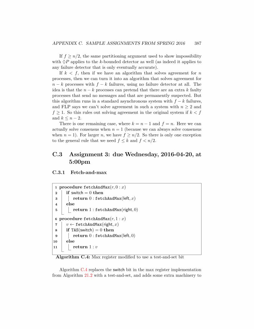
APPENDIX C. SAMPLE ASSIGNMENTS FROM SPRING 2016 387

If f ≥ n/2, the same partitioning argument used to show impossibilitywith ♦P applies to the k-bounded detector as well (as indeed it applies toany failure detector that is only eventually accurate).

If k < f , then if we have an algorithm that solves agreement for nprocesses, then we can turn it into an algorithm that solves agreement forn − k processes with f − k failures, using no failure detector at all. Theidea is that the n− k processes can pretend that there are an extra k faultyprocesses that send no messages and that are permanently suspected. Butthis algorithm runs in a standard asynchronous system with f − k failures,and FLP says we can’t solve agreement in such a system with n ≥ 2 andf ≥ 1. So this rules out solving agreement in the original system if k < fand k ≤ n− 2.

There is one remaining case, where k = n− 1 and f = n. Here we canactually solve consensus when n = 1 (because we can always solve consensuswhen n = 1). For larger n, we have f ≥ n/2. So there is only one exceptionto the general rule that we need f ≤ k and f < n/2.

C.3 Assignment 3: due Wednesday, 2016-04-20, at5:00pm

C.3.1 Fetch-and-max

1 procedure fetchAndMax(r, 0 : x)2 if switch = 0 then3 return 0 : fetchAndMax(left, x)4 else5 return 1 : fetchAndMax(right, 0)

6 procedure fetchAndMax(r, 1 : x)7 v ← fetchAndMax(right, x)8 if TAS(switch) = 0 then9 return 0 : fetchAndMax(left, 0)

10 else11 return 1 : v

Algorithm C.4: Max register modified to use a test-and-set bit

Algorithm C.4 replaces the switch bit in the max register implementationfrom Algorithm 21.2 with a test-and-set, and adds some extra machinery to

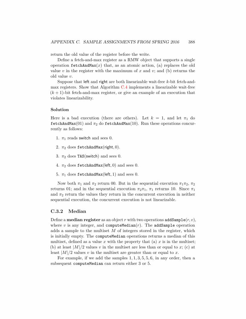
APPENDIX C. SAMPLE ASSIGNMENTS FROM SPRING 2016 388

return the old value of the register before the write.Define a fetch-and-max register as a RMW object that supports a single

operation fetchAndMax(x) that, as an atomic action, (a) replaces the oldvalue v in the register with the maximum of x and v; and (b) returns theold value v.

Suppose that left and right are both linearizable wait-free k-bit fetch-and-max registers. Show that Algorithm C.4 implements a linearizable wait-free(k + 1)-bit fetch-and-max register, or give an example of an execution thatviolates linearizability.

Solution

Here is a bad execution (there are others). Let k = 1, and let π1 dofetchAndMax(01) and π2 do fetchAndMax(10). Run these operations concur-rently as follows:

1. π1 reads switch and sees 0.

2. π2 does fetchAndMax(right, 0).

3. π2 does TAS(switch) and sees 0.

4. π2 does fetchAndMax(left, 0) and sees 0.

5. π1 does fetchAndMax(left, 1) and sees 0.

Now both π1 and π2 return 00. But in the sequential execution π1π2, π2returns 01; and in the sequential execution π2π1, π1 returns 10. Since π1and π2 return the values they return in the concurrent execution in neithersequential execution, the concurrent execution is not linearizable.

C.3.2 Median

Define amedian register as an object r with two operations addSample(r, v),where v is any integer, and computeMedian(r). The addSample operationadds a sample to the multiset M of integers stored in the register, whichis initially empty. The computeMedian operations returns a median of thismultiset, defined as a value x with the property that (a) x is in the multiset;(b) at least |M |/2 values v in the multiset are less than or equal to x; (c) atleast |M |/2 values v in the multiset are greater than or equal to x.

For example, if we add the samples 1, 1, 3, 5, 5, 6, in any order, then asubsequent computeMedian can return either 3 or 5.

APPENDIX C. SAMPLE ASSIGNMENTS FROM SPRING 2016 389

Suppose that you wish to implement a linearizable wait-free medianregister using standard atomic registers and resettable test-and-set bits. Givetight (up to constants) asymptotic upper and lower bounds on the numberof such objects you would need. You may assume that the atomic registersmay hold arbitrarily large values.

Solution

For the upper bound, we can do it with O(n) registers using any linear-spacesnapshot algorithm (for example, Afek et al. [AAD+93]). Each process storesin its own segment of the snapshot object the multiset of all samples addedby that process; addSample just adds a new sample to the process’s segment.For computeMedian, take a snapshot, then take the union of all the multisets,then compute the median of this union. Linearizability and wait-freedomof both operations are immediate from the corresponding properties of thesnapshot object.

For the lower bound, use JTT [JTT00]. Observe that both atomicregisters and resettable test-and-sets are historyless: for both types, the newstate after an operation doesn’t depend on the old state. So JTT applies ifwe can show that the median register is perturbable.

Suppose that we have a schedule ΛkΣkπ in which Λk consists of anarbitrary number of median-register operations of which at most k areincomplete, Σk consists of k pending base object operations (writes, test-and-sets, or test-and-set resets) covering k distinct base objects, and π is a readoperation by a process not represented in ΛkΣk. We need to find a sequenceof operations γ that can be inserted between Λk and Σk that changes theoutcome of π.

Let S be the multiset of all values appearing as arguments to addSampleoperations that start in Λk or Σk. Let x = maxS (or 0 if S is empty), and letγ consist of |S|+ 1 addSample(r, x+ 1) operations. Write T for the multisetof |S|+ 1 copies of x+ 1. Then in any linearization of ΛkγΣkπ, the multisetU of samples contained in r when π executes includes at least all of T and atmost all of S; this means that a majority of values in U are equal to x+ 1,and so the median is x + 1. But x + 1 does not appear in S, so π can’treturn it in ΛkΣkπ. It follows that a median register is in fact perturbable,and JTT applies, which means that we need at least Ω(n) base objects toimplement a median register.

APPENDIX C. SAMPLE ASSIGNMENTS FROM SPRING 2016 390

C.3.3 Randomized two-process test-and-set with small reg-isters

Algorithm C.5 gives an implementation of a randomized one-shot test-and-setfor two processes, each of which may call the procedure at most once, withits process id (0 or 1) as an argument.

The algorithm uses two registers, a0 and a1, that are both initializedto 0 and hold values in the range 0 . . .m− 1, where m is a positive integer.Unfortunately, whoever wrote it forgot to specify the value of m.

1 procedure TAS(i)2 myPosition← 03 while true do4 otherPosition← read(a¬i)5 x← myPosition− otherPosition6 if x ≡ 2 (mod m) then7 return 08 else if x ≡ −1 (mod m) do9 return 1

10 else if fair coin comes up heads do11 myPosition← (myPosition + 1) mod m12 write(ai,myPosition)

Algorithm C.5: Randomized one-shot test-and-set for two processes

For what values of m does Algorithm C.5 correctly implement a one-shot,probabilistic wait-free, linearizable test-and-set, assuming:

1. An oblivious adversary?

2. An adaptive adversary?

Solution

For the oblivious adversary, we can quickly rule out m < 5, by showing thatthere is an execution in each case where both processes return 0:

• When m = 1 or m = 2, both processes immediately return 0, becausethe initial difference 0 is congruent to 2 mod m.

• When m = 3, there is an execution in which p0 writes 1 to a0, p1 readsthis 1 and computes x = −1 ≡ 2 (mod 3) and returns 0, then p0 reads

APPENDIX C. SAMPLE ASSIGNMENTS FROM SPRING 2016 391

0 from a0, computes x = 1, advances a0 to 2, then re-reads 0 from a0,computes x = 2, and returns 0.

• When m = 4, run p0 until it writes 2 to a0. It then computes x = 2and returns 0. If we now wake up p1, it computes x = −2 ≡ 2 (mod 4)and also returns 0.

When m ≥ 5 and the adversary is oblivious, the implementation works.We need to show both linearizability and termination. We’ll start withlinearizability.

Observe that in a sequential execution, first process to perform TASreturns 0 and the second 1. So we need to show (a) that the processesbetween them return both values, and (b) that if one process finishes beforethe other starts, the first process returns 0.

It is immediate from Algorithm C.5 that in any reachable configuration,myPositioni ∈ ai, ai + 1, because process i can only increment myPositionat most once before writing its value to ai.

Below we will assume without loss of generality that p0 is the first processto perform its last read before returning.

Suppose that p0 returns 0. This means that p0 observed a1 ≡ a0 − 2(mod m). So at the time p0 last read a1, myPosition1 was congruent to eithera0 − 1 or a0 − 2. This means that on its next read of a0, p1 will compute xcongruent to either −1 or −2. Because m is at least 5, in neither case willit mistake this difference for 2. If it computed x ≡ −1, it returns 1; if itcomputed x ≡ −2, it does not return immediately, but eventually it will flipits coin heads, increment myPosition1, and return 1. In either case we havethat exactly one process returns each value.

Alternatively, suppose that p0 returns 1. Then p0 reads a1 ≡ a0 + 1,and at the time of this read, myPosition1 is either congruent to a0 + 1 ora0 + 2. In the latter case, p1 returns 0 after its next read; in the former,p1 eventually increments myPosition1 and then returns 0. In either case weagain have that exactly one process returns each value.

Now suppose that p0 runs to completion before p1 starts. Initially, p0sees a0 ≡ a1, but eventually p0 increments a0 enough times that a0 − a1 ≡ 2;p0 returns 0.

To show termination (with probability 1), consider any configuration inwhich neither process has returned. During the next 2k steps, at least oneprocess takes k steps. Suppose that during this interval, this fast processincrements myPosition at every opportunity, while the other process doesnot increment myPosition at all (this event occurs with nonzero probability

APPENDIX C. SAMPLE ASSIGNMENTS FROM SPRING 2016 392

for any fixed k, because the coin-flips are uncorrelated with the obliviousadversary’s choice of which process is fast). Then for k sufficiently large, thefast process eventually sees a0 − a1 congruent to either 2 or −1 and returns.Since this event occurs with independent nonzero probability in each intervalof length 2k, eventually it occurs.2

Once one process has terminated, the other increments myPosition in-finitely often, so it too eventually sees a gap of 2 or −1.

For the adaptive adversary, the adversary can prevent the algorithm fromterminating. Starting from a state in which both processes are about toread and a0 = a1 = k, run p0 until it is about to write (k + 1) mod m to a0(unlike the oblivious adversary, the adaptive adversary can see when this willhappen). Then run p1 until it is about to write (k + 1) mod m to a1. Letboth writes go through. We are now in a state in which both processes areabout to read, and a0 = a1 = (k + 1) mod m. So we can repeat this strategyforever.

C.4 Presentation (for students taking CPSC 565):due Wednesday, 2016-04-27

Students taking CPSC 565, the graduate version of the class, are expected togive a 15-minute presentation on a recent paper in the theory of distributedcomputing.

The choice of paper to present should be made in consultation with theinstructor. To a first approximation, any paper from PODC, DISC, or asimilar conference in the last two or three years (that is not otherwise coveredin class) should work.

Because of the limited presentation time, you are not required to getinto all of the technical details of the paper, but your presentation shouldinclude3

1. Title, authors, and date and venue of publication of the paper.

2. A high-level description of the main result. Unlike a talk for a general2The fancy way to prove this is to invoke the second Borel-Cantelli lemma of probability

theory. Or we can just argue that the probability that we don’t terminate in the first `intervals is at most (1− ε)`, which goes to zero in the limit.

3Literary theorists will recognize this as a three-act structure (preceded by a title card):introduce the main character, make their life difficult, then resolve their problems in timefor the final curtain. This is not the only way to organize a talk, but if done right it hasthe advantage of keeping the audience awake.

APPENDIX C. SAMPLE ASSIGNMENTS FROM SPRING 2016 393

audience, you can assume that your listeners know at least everythingthat we’ve talked about so far in the class.

3. A description of where this result fits into the literature (e.g., solvesan open problem previously proposed in [...], improves on the previousbest running time for an algorithm from [...], gives a lower bound orimpossibility result for a problem previously proposed by [...], opensup a new area of research for studying [...]), and why it is interestingand/or hard.

4. A description (also possibly high-level) of the main technical mecha-nism(s) used to get the main result.

You do not have to prepare slides for your presentation if you wouldprefer to use the blackboard, but you should make sure to practice it inadvance to make sure it fits in the allocated time. The instructor will behappy to offer feedback on draft versions if available far enough before theactual presentation date.

Relevant dates:

2016-04-13 Paper selection due.

2016-04-22 Last date to send draft slides or arrange for a practice presen-tation with the instructor if you want guaranteed feedback.

2016-04-27 Presentations, during the usual class time.

C.5 CS465/CS565 Final Exam, May 10th, 2016Write your answers in the blue book(s). Justify your answers. Work alone.Do not use any notes or books.

There are four problems on this exam, each worth 20 points, for a totalof 80 points. You have approximately three hours to complete this exam.

C.5.1 A slow register (20 points)

Define a second-to-last register as having a read operation that alwaysreturns the second-to-last value written to it. For example, after write (1),write (2), write (3), a subsequent read operation will return 2. If fewerthat two write operations have occurred, a read will return ⊥.

What is the consensus number of this object?

APPENDIX C. SAMPLE ASSIGNMENTS FROM SPRING 2016 394

Solution

The consensus number of this object is 2.For two processes, have each process i write its input to a standard

atomic register r[i], and then write its id to a shared second-to-last-valueregister s. We will have whichever process writes to s first win. After writing,process i can detect which process wrote first by reading s once, becauseit either sees ⊥ (meaning the other process has not written yet) or it seesthe identity of the process that wrote first. In either case it can return thewinning process’s input.

For three processes, the usual argument gets us to a configuration Cwhere all three processes are about to execute operations x, y, and z onthe same object, where each operation moves from a bivalent to a univalentstate. Because we know that this object can’t be a standard atomic register,it must be a second-to-last register. We can also argue that all of x, y, andz are writes, because if one of them is not, the processes that don’t performit can’t tell if it happened or not.

Suppose that Cx is 0-valent and Cy is 1-valent. Then Cxyz is 0-valentand Cyz is 1-valent. But these configurations are indistinguishable to anyprocess but x. It follows that the second-to-last register can’t solve consensusfor three processes.

C.5.2 Two leaders (20 points)

Assume that you are working in an asynchronous message-passing systemorganized as a connected graph, where all processes run the same code exceptthat each process starts with an id and the knowledge of the ids of all of itsneighbors. Suppose that all of these ids are unique, except that the smallestid (whatever it is) might appear on either one or two processes.

Is it possible in all cases to detect which of these situations hold? Eithergive an algorithm that allows all processes to eventually correctly returnwhether there are one or two minimum-id processes in an arbitrary connectedgraph, or show that no such algorithm is possible.

Solution

Here is an algorithm.If there are two processes p and q with the same id that are adjacent to

each other, they can detect this in the initial configuration, and transmitthis fact to all the other processes by flooding.

APPENDIX C. SAMPLE ASSIGNMENTS FROM SPRING 2016 395

If these processes p and q are not adjacent, we will need some othermechanism to detect them. Define the extended id of a process as its own idfollowed by a list of the ids of its neighbors in some fixed order. Order theextended ids lexicographically, so that a process with a smaller id also has asmaller extended id.

Suppose now that p and q are not adjacent and have the same extendedid. Then they share the same neighbors, and each of these neighbors will seethat p and q have duplicate ids. So we can do an initial round of messageswhere each process transmits its extended id to its neighbors, and if p and qobserve that their id is a duplicate, they can again notify all the processes toreturn that there are two leaders by flooding.

The remaining case is that p and q have distinct extended ids, or thatonly one minimum-process id exists. In either case we can run any standardbroadcast-based leader-election algorithm, using the extended ids, which willleave us with a tree rooted at whichever process has the minimum extendedid. This process can then perform convergecast to detect if there is anotherprocess with the same id, and perform broadcast to inform all processes ofthis fact.

C.5.3 A splitter using one-bit registers (20 points)

Algorithm C.6 implements a splitter-like object using one-bit registers. Itassumes that each process has a unique id id consisting of k = dlgne bitsidk−1idk−2 . . . id0. We would like this object to have the properties that (a)if exactly one process executes the algorithm, then it wins; and (b) in anyexecution, at most one process wins.

Show that the algorithm has these properties, or give an example of anexecution where it does not.

Solution

The implementation is correct.If one process runs alone, it sets A[i][idi] for each i, sees 0 in door, then

sees 0 in each location A[i][¬idi] and wins. So we have property (a).Now suppose that some process with id p wins in an execution that may

involve other processes. Then p writes A[i][pi] for all i before observing 0 indoor, which means that it sets all these bits before any process writes 1 todoor. If some other process q also wins, then there is at least one position iwhere pi = ¬qi, and q reads A[i][pi] after writing 1 to door. But then q sees1 in this location and loses, a contradiction.

APPENDIX C. SAMPLE ASSIGNMENTS FROM SPRING 2016 396

shared data:1 one-bit atomic registers A[i][j] for i = 0 . . . dlgne − 1 and j ∈ 0, 1,

all initially 02 one-bit atomic register door, initially 03 procedure splitter(id)4 for i← 0 to k − 1 do5 A[i][idi]← 16 if door = 1 then7 return lose8 door← 19 for i← 0 to k − 1 do

10 if A[i][¬idi] = 1 then11 return lose

12 return win

Algorithm C.6: Splitter using one-bit registers

C.5.4 Symmetric self-stabilizing consensus (20 points)

Suppose we have a synchronous system consisting of processes organized in aconnected graph. The state of each process is a single bit, and each processcan directly observe the number of neighbors that it has and how many ofthem have 0 bits and how many have 1 bits. At each round, a process countsthe number of neighbors k0 with zeros, the number k1 with ones, and itsown bit b, and chooses a new bit for the next round f(b, k0, k1) according tosome rule f that is the same for all processes. The goal of the processes isto reach consensus, where all processes have the same bit forever, startingfrom an arbitrary initial configuration. An example of a rule that has thisproperty is for f to output 1 if b = 1 or k1 > 0.

However, this rule is not symmetric with respect to bit values: if wereplace all ones by zeros and vice versa, we get different behavior.

Prove or disprove: There exists a rule f that is symmetric, by which wemean that f(b, k0, k1) = ¬f(¬b, k1, k0) always, such that applying this rulestarting from an arbitrary configuration in an arbitrary graph eventuallyconverges to all processes having the same bit forever.

APPENDIX C. SAMPLE ASSIGNMENTS FROM SPRING 2016 397

Solution

Disproof by counterexample: Fix some f , and consider a graph with twoprocesses p0 and p1 connected by an edge. Let p0 start with 0 and p1 startwith 1. Then p0’s next state is f(0, 0, 1) = ¬f(1, 1, 0) 6= f(1, 1, 0), which isp1’s next state. So either p0 still has 0 and p1 still has 1, in which case wenever make progress; or they swap their bits, in which case we can apply thesame analysis with p0 and p1 reversed to show that they continue to swapback and forth forever. In either case the system does not converge.

Appendix D

Sample assignments fromSpring 2014

D.1 Assignment 1: due Wednesday, 2014-01-29, at5:00pm

Bureaucratic part

Send me email! My address is james.aspnes@gmail.com.In your message, include:

1. Your name.

2. Your status: whether you are an undergraduate, grad student, auditor,etc.

3. Anything else you’d like to say.

(You will not be graded on the bureaucratic part, but you should do itanyway.)

D.1.1 Counting evil processes

A connected bidirectional asynchronous network of n processes with identitieshas diameter D and may contain zero or more evil processes. Fortunately,the evil processes, if they exist, are not Byzantine, fully conform to RFC3514 [Bel03], and will correctly execute any code we provide for them.

Suppose that all processes wake up at time 0 and start whatever protocolwe have given them. Suppose that each process initially knows whether it is

398

APPENDIX D. SAMPLE ASSIGNMENTS FROM SPRING 2014 399

evil, and knows the identities of all of its neighbors. However, the processesdo not know the number of processes n or the diameter of the network D.

Give a protocol that allows every process to correctly return the numberof evil processes no later than time D. Your protocol should only return avalue once for each process (no converging to the correct answer after aninitial wrong guess).

Solution

There are a lot of ways to do this. Since the problem doesn’t ask aboutmessage complexity, we’ll do it in a way that optimizes for algorithmicsimplicity.

At time 0, each process initiates a separate copy of the flooding algorithm(Algorithm 3.1). The message 〈p,N(p), e〉 it distributes consists of its ownidentity, the identities of all of its neighbors, and whether or not it is evil.

In addition to the data for the flooding protocol, each process tracks aset I of all processes it has seen that initiated a protocol and a set N of allprocesses that have been mentioned as neighbors. The initial values of thesesets for process p are p and N(p), the neighbors of p.

Upon receiving a message 〈q,N(q), e〉, a process adds q to I and N(q) toN . As soon as I = N , the process returns a count of all processes for whiche = true.

Termination by D: Follows from the same analysis as flooding. Anyprocess at distance d from p has p ∈ I by time d, so I is complete by time D.

Correct answer: Observe that N =⋃i∈I N(i) always. Suppose that there

is some process q that is not in I. Since the graph is connected, there is apath from p to q. Let r be the last node in this path in I, and let s be thefollowing node. Then s ∈ N \ I and N 6= I. By contraposition, if I = Nthen I contains all nodes in the network, and so the count returned at thistime is correct.

D.1.2 Avoiding expensive processes

Suppose that you have a bidirectional but not necessarily complete asyn-chronous message-passing network represented by a graph G = (V,E) whereeach node in V represents a process and each edge in E connects two pro-cesses that can send messages to each other. Suppose further that eachprocess is assigned a weight 1 or 2. Starting at some initiator process, we’dlike to construct a shortest-path tree, where each process points to one of

APPENDIX D. SAMPLE ASSIGNMENTS FROM SPRING 2014 400

its neighbors as its parent, and following the parent pointers always gives apath of minimum total weight to the initiator.1

Give a protocol that solves this problem with reasonable time, message,and bit complexity, and show that it works.

Solution

There’s an ambiguity in the definition of total weight: does it include theweight of the initiator and/or the initial node in the path? But since thesevalues are the same for all paths to the initiator from a given process, theydon’t affect which is lightest.

If we don’t care about bit complexity, there is a trivial solution: Use anexisting BFS algorithm followed by convergecast to gather the entire structureof the network at the initiator, run your favorite single-source shortest-pathalgorithm there, then broadcast the results. This has time complexity O(D)and message complexity O(DE) if we use the BFS algorithm from §4.3. Butthe last couple of messages in the convergecast are going to be pretty big.

A solution by reduction: Suppose that we construct a new graph G′

where each weight-2 node u in G is replaced by a clique of nodes u1, u2, . . . uk,with each node in the clique attached to a different neighbor of u. We thenrun any breadth-first search protocol of our choosing on G′, where eachweight-2 node simulates all members of the corresponding clique. Becauseany path that passes through a clique picks up an extra edge, each path inthe breadth-first search tree has a length exactly equal to the sum of theweights of the nodes other than its endpoints.

A complication is that if I am simulating k nodes, between them theymay have more than one parent pointer. So we define u.parent to be ui.parentwhere ui is a node at minimum distance from the initiator in G′. We alsore-route any incoming pointers to uj 6= ui to point to ui instead. Because uiwas chosen to have minimum distance, this never increases the length of anypath, and the resulting modified tree is a still a shortest-path tree.

Adding nodes blows up |E′|, but we don’t need to actually send messagesbetween different nodes ui represented by the same process. So if we use the§4.3 algorithm again, we only send up to D messages per real edge, givingO(D) time and O(DE) messages.

If we don’t like reductions, we could also tweak one of our existingalgorithms. Gallager’s layered BFS (§4.2) is easily modified by changing the

1Clarification added 2014-01-26: The actual number of hops is not relevant for theconstruction of the shortest-path tree. By shortest path, we mean path of minimum totalweight.

APPENDIX D. SAMPLE ASSIGNMENTS FROM SPRING 2014 401

depth bound for each round to a total-weight bound. The synchronizer-basedBFS can also be modified to work, but the details are messy.

D.2 Assignment 2: due Wednesday, 2014-02-12, at5:00pm

D.2.1 Synchronous agreement with weak failures

Suppose that we modify the problem of synchronous agreement with crashfailures from Chapter 9 so that instead of crashing a process forever, theadversary may jam some or all of its outgoing messages for a single round.The adversary has limited batteries on its jamming equipment, and canonly cause f such one-round faults. There is no restriction on when theseone-round jamming faults occur: the adversary might jam f processes forone round, one process for f rounds, or anything in between, so long as thesum over all rounds of the number of processes jammed in each round is atmost f . For the purposes of agreement and validity, assume that a processis non-faulty if it is never jammed.2

As a function of f and n, how many rounds does it take to reach agreementin the worst case in this model, under the usual assumptions that processesare deterministic and the algorithm must satisfy agreement, termination,and validity? Give the best upper and lower bounds that you can.

Solution

The par solution for this is an Ω(√f) lower bound and O(f) upper bound. I

don’t know if it is easy to do better than this.For the lower bound, observe that the adversary can simulate an ordinary

crash failure by jamming a process in every round starting in the round itcrashes in. This means that in an r-round protocol, we can simulate k crashfailures with kr jamming faults. From the Dolev-Strong lower bound [DS83](see also Chapter 9), we know that there is no r-round protocol with k = rcrash failures faults, so there is no r-round protocol with r2 jamming faults.This gives a lower bound of b

√fc+ 1 on the number of rounds needed to

solve synchronous agreement with f jamming faults.3

2Clarifications added 2014-02-10: We assume that processes don’t know that they arebeing jammed or which messages are lost (unless the recipient manages to tell them that amessage was not delivered). As in the original model, we assume a complete network andthat all processes have known identities.

3Since Dolev-Strong only needs to crash one process per round, we don’t really need

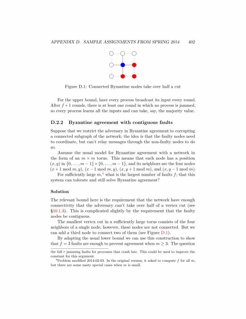
APPENDIX D. SAMPLE ASSIGNMENTS FROM SPRING 2014 402

Figure D.1: Connected Byzantine nodes take over half a cut

For the upper bound, have every process broadcast its input every round.After f + 1 rounds, there is at least one round in which no process is jammed,so every process learns all the inputs and can take, say, the majority value.

D.2.2 Byzantine agreement with contiguous faults

Suppose that we restrict the adversary in Byzantine agreement to corruptinga connected subgraph of the network; the idea is that the faulty nodes needto coordinate, but can’t relay messages through the non-faulty nodes to doso.

Assume the usual model for Byzantine agreement with a network inthe form of an m × m torus. This means that each node has a position(x, y) in 0, . . . ,m− 1×0, . . . ,m− 1, and its neighbors are the four nodes(x+ 1 mod m, y), (x− 1 mod m, y), (x, y + 1 mod m), and (x, y− 1 mod m).

For sufficiently large m,4 what is the largest number of faults f ; that thissystem can tolerate and still solve Byzantine agreement?

Solution

The relevant bound here is the requirement that the network have enoughconnectivity that the adversary can’t take over half of a vertex cut (see§10.1.3). This is complicated slightly by the requirement that the faultynodes be contiguous.

The smallest vertex cut in a sufficiently large torus consists of the fourneighbors of a single node; however, these nodes are not connected. But wecan add a third node to connect two of them (see Figure D.1).

By adapting the usual lower bound we can use this construction to showthat f = 3 faults are enough to prevent agreement whenm ≥ 3. The question

the full r jamming faults for processes that crash late. This could be used to improve theconstant for this argument.

4Problem modified 2014-02-03. In the original version, it asked to compute f for all m,but there are some nasty special cases when m is small.

APPENDIX D. SAMPLE ASSIGNMENTS FROM SPRING 2014 403

then is whether f = 2 faults is enough.By a case analysis, we can show that any two nodes in a sufficiently large

torus are either adjacent themselves or can be connected by three paths,where no two paths have adjacent vertices. Assume without loss of generalitythat one of the nodes is at position (0, 0). Then any other node is coveredby one of the following cases:

1. Nodes adjacent to (0, 0). These can communicate directly.

2. Nodes at (0, i) or (i, 0). These cases are symmetric, so we’ll describe thesolution for (0, i). Run one path directly north: (0, 1), (0, 2), . . . , (0, i−1). Similarly, run a second path south: (0,−1), (0,−2), . . . (0, i + 1).For the third path, take two steps east and then run north and backwest: (1, 0), (2, 0), (2, 1), (2, 2), . . . , (2, i), (1, i). These paths are all non-adjacent as long as m ≥ 4.

3. Nodes at (±1, i) or (i,±1), where i is not −1, 0, or 1. Suppose the nodeis at (1, i). Run one path east then north through (1, 0), (1, 1), . . . , (1, i−1). The other two paths run south and west, with a sideways jog in themiddle as needed. This works for m sufficiently large to make roomfor the sideways jogs.

4. Nodes at (±1,±1) or (i, j) where neither of i or j is −1, 0, or 1. Nowwe can run one path north then east, one east then north, one souththen west, and one west then south, creating four paths in a figure-eightpattern centered on (0, 0).

D.3 Assignment 3: due Wednesday, 2014-02-26, at5:00pm

D.3.1 Among the elect

The adversary has decided to be polite and notify each non-faulty processeswhen he gives up crashing it. Specifically, we have the usual asynchronousmessage-passing system with up to f faulty processes, but every non-faultyprocess is eventually told that it is non-faulty. (Faulty processes are toldnothing.)

For what values of f can you solve consensus in this model?

Solution

We can tolerate f < n/2, but no more.

APPENDIX D. SAMPLE ASSIGNMENTS FROM SPRING 2014 404

If f < n/2, the following algorithm works: Run Paxos, where eachprocess i waits to learn that it is non-faulty, then acts as a proposer forproposal number i. The highest-numbered non-faulty process then carriesout a proposal round that succeeds because no higher proposal is ever issued,and both the proposer (which is non-faulty) and a majority of acceptersparticipate.

If f ≥ n/2, partition the processes into two groups of size bn/2c, withany leftover process crashing immediately. Make all of the processes in bothgroups non-faulty, and tell each of them this at the start of the protocol.Now do the usual partitioning argument: Run group 0 with inputs 0 withno messages delivered from group 1 until all processes decide 0 (we can dothis because the processes can’t distinguish this execution from one in whichthe group 1 processes are in fact faulty). Run group 1 similarly until allprocesses decide 1. We have then violated agreement, assuming we didn’tpreviously violate termination of validity.

D.3.2 Failure detectors on the cheap

Suppose we do not have the budget to equip all of our machines with failuredetectors. Instead, we order an eventually strong failure detector for kmachines, and the remaining n− k machines get fake failure detectors thatnever suspect anybody. The choice of which machines get the real failuredetectors and which get the fake ones is under the control of the adversary.

This means that every faulty process is eventually permanently suspectedby every non-faulty process with a real failure detector, and there is atleast one non-faulty process that is eventually permanently not suspected byanybody. Let’s call the resulting failure detector ♦Sk.

Let f be the number of actual failures. Under what conditions on f , k,and n can you still solve consensus in the usual deterministic asynchronousmessage-passing model using ♦Sk?

Solution

First observe that ♦S can simulate ♦Sk for any k by having n− k processesignore the output of their failure detectors. So we need f < n/2 by the usuallower bound on ♦S.

If f ≥ k, we are also in trouble. The f > k case is easy: If there existsa consensus protocol for f > k, then we can transform it into a consensusprotocol for n−k processes and f−k failures, with no failure detectors at all,by pretending that there are an extra k processes with real failure detectors

APPENDIX D. SAMPLE ASSIGNMENTS FROM SPRING 2014 405

that crash immediately. The FLP impossibility result rules this out.If f = k, we have to be a little more careful. By immediately crashing

f − 1 processes with real failure detectors, we can reduce to the f = k = 1case. Now the adversary runs the FLP strategy. If no processes crash, thenall n− k + 1 surviving process report no failures; if it becomes necessary tocrash a process, this becomes the one remaining process with the real failuredetector. In either case the adversary successfully prevents consensus.

So let f < k. Then we have weak completeness, because every faultyprocess is eventually permanently suspected by at least k − f > 0 processes.We also have weak accuracy, because it is still the case that some processis eventually permanently never suspected by anybody. By boosting weakcompleteness to strong completeness as described in §13.2.3, we can turnout failure detector into ♦S, meaning we can solve consensus precisely whenf < min(k, n/2).

D.4 Assignment 4: due Wednesday, 2014-03-26, at5:00pm

D.4.1 A global synchronizer with a global clock

Consider an asynchronous message-passing system with n processes in abidirectional ring with no failures. Suppose that the processes are equippedwith a global clock, which causes a local event to occur simultaneously ateach process every c time units, where as usual 1 is the maximum messagedelay. We would like to use this global clock to build a global synchronizer.Provided c is at least 1, a trivial approach is to have every process advanceto the next round whenever the clock pulse hits. This gives one synchronousround every c time units.

Suppose that c is greater than 1 but still o(n). Is it possible to build aglobal synchronizer in this model that runs more than a constant ratio fasterthan this trivial global synchronizer in the worst case?

Solution

No. We can adapt the lower bound on the session problem from §7.4.2 toapply in this model.

Consider an execution of an algorithm for the session problem in whicheach message is delivered exactly one time unit after it is sent. Divideit as in the previous proof into a prefix β containing special actions anda suffix δ containing no special actions. Divide β further into segments

APPENDIX D. SAMPLE ASSIGNMENTS FROM SPRING 2014 406

β1, β2, β3, . . . , βk, where each segment ends with a clock pulse. Followingthe standard argument, because each segment has duration less than thediameter of the network, there is no causal connection between any specialactions done by processes at opposite ends of the network that are in thesame segment βi. So we can causally shuffle each βi to get a new segment β′iwhere all special actions of process p0 (say) occur before all special actionsof process pn/2. This gives at most one session per segment, or at most onesession for every c time units.

Since a globally synchronous system can do one session per round, thismeans that our global synchronizer can only produce one session per c timeunits as well.

D.4.2 A message-passing counter

A counter is a shared object that support operations inc and read, whereread returns the number of previous inc operations.

Algorithm D.1 purports to implement a counter in an asynchronousmessage-passing system subject to f < n/2 crash failures. In the algorithm,each process i maintains a vector ci of contributions to the counter from allthe processes, as well as a nonce ri used to distinguish responses to differentread operations from each other. All of these values are initially zero.

Show that the implemented counter is linearizable, or give an example ofan execution where it isn’t.

Solution

This algorithm is basically implementing an array of ABD registers [ABND95],but it omits the second phase on a read where any information the readerlearns is propagated to a majority. So we expect it to fail the same way ABDwould without this second round, by having two read operations returnvalues that are out of order with respect to their observable ordering.

Here is one execution that produces this bad outcome:

1. Process p1 starts an inc by updating c1[1] to 1.

2. Process p2 carries out a read operation in which it receives responsesfrom p1 and p2, and returns 1.

3. After p2 finishes, process p3 carries out a read operation in which itreceives responses from p2 and p3, and returns 0.

APPENDIX D. SAMPLE ASSIGNMENTS FROM SPRING 2014 407

1 procedure inc2 ci[i]← ci[i] + 13 Send ci[i] to all processes.4 Wait to receive ack(ci[i]) from a majority of processes.5 upon receiving c from j do6 ci[j]← max(ci[j], c)7 Send ack(c) to j.8 procedure read9 ri ← ri + 1

10 Send read(ri) to all processes.11 Wait to receive respond(ri, cj) from a majority of processes j.12 return

∑k maxj cj [k]

13 upon receiving read(r) from j do14 Send respond(r, ci) to j

Algorithm D.1: Counter algorithm for Problem D.4.2.

If we want to be particularly perverse, we can exploit the fact that p2doesn’t record what it learns in its first read to have p2 do the second readthat returns 0 instead of p3. This shows that Algorithm D.1 isn’t evensequentially consistent.

The patch, if we want to fix this, is to include the missing second phasefrom ABD in the read operation: after receiving values from a majority, Iset ci[k] to maxj cj [k] and send my updated values to a majority. That theresulting counter is linearizable is left as an exercise.

D.5 Assignment 5: due Wednesday, 2014-04-09, at5:00pm

D.5.1 A concurrency detector

Consider the following optimistic mutex-like object, which we will call aconcurrency detector. A concurrency detector supports two operationsfor each process i, enteri and exiti. These operations come in pairs: aprocess enters a critical section by executing enteri, and leaves by executingexiti. The behavior of the object is undefined if a process calls enteri twicewithout an intervening exiti, or calls exiti without first calling enteri.

Unlike mutex, a concurrency detector does not enforce that only one

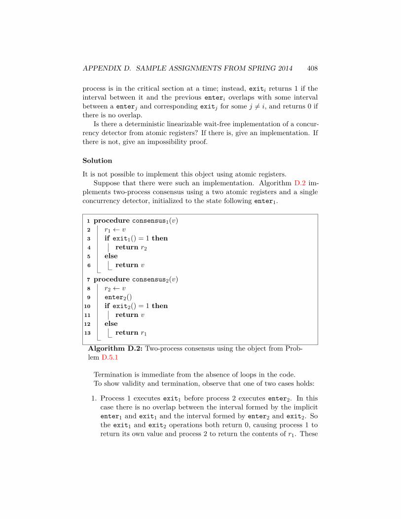
APPENDIX D. SAMPLE ASSIGNMENTS FROM SPRING 2014 408

process is in the critical section at a time; instead, exiti returns 1 if theinterval between it and the previous enteri overlaps with some intervalbetween a enterj and corresponding exitj for some j 6= i, and returns 0 ifthere is no overlap.

Is there a deterministic linearizable wait-free implementation of a concur-rency detector from atomic registers? If there is, give an implementation. Ifthere is not, give an impossibility proof.

Solution

It is not possible to implement this object using atomic registers.Suppose that there were such an implementation. Algorithm D.2 im-

plements two-process consensus using a two atomic registers and a singleconcurrency detector, initialized to the state following enter1.

1 procedure consensus1(v)2 r1 ← v3 if exit1() = 1 then4 return r25 else6 return v

7 procedure consensus2(v)8 r2 ← v9 enter2()

10 if exit2() = 1 then11 return v12 else13 return r1

Algorithm D.2: Two-process consensus using the object from Prob-lem D.5.1

Termination is immediate from the absence of loops in the code.To show validity and termination, observe that one of two cases holds:

1. Process 1 executes exit1 before process 2 executes enter2. In thiscase there is no overlap between the interval formed by the implicitenter1 and exit1 and the interval formed by enter2 and exit2. Sothe exit1 and exit2 operations both return 0, causing process 1 toreturn its own value and process 2 to return the contents of r1. These

APPENDIX D. SAMPLE ASSIGNMENTS FROM SPRING 2014 409

will equal process 1’s value, because process 2’s read follows its call toenter2, which follows exit1 and thus process 1’s write to r1.

2. Process 1 executes exit1 after process 2 executes enter2. Now bothexit operations return 1, and so process 2 returns its own value whileprocess 1 returns the contents of r2, which it reads after process 2writes its value there.

In either case, both processes return the value of the first process to accessthe concurrency detector, satisfying both agreement and validity. This wouldgive a consensus protocol for two processes implemented from atomic registers,contradicting the impossibility result of Loui and Abu-Amara [LAA87].

D.5.2 Two-writer sticky bits

A two-writer sticky bit is a sticky bit that can be read by any process,but that can only be written to by two specific processes.

Suppose that you have an unlimited collection of two-writer sticky bitsfor each pair of processes, plus as many ordinary atomic registers as youneed. What is the maximum number of processes for which you can solvewait-free binary consensus?

Solution

If n = 2, then a two-writer sticky bit is equivalent to a sticky bit, so we cansolve consensus.

If n ≥ 3, suppose that we maneuver our processes as usual to a bivalentconfiguration C with no bivalent successors. Then there are three pendingoperations x, y, and z, that among them produce both 0-valent and 1-valentconfigurations. Without loss of generality, suppose that Cx and Cy are both0-valent and Cz is 1-valent. We now consider what operations these mightbe.

1. If x and z apply to different objects, then Cxz = Czx must be both0-valent and 1-valent, a contradiction. Similarly if y and z apply todifferent objects. This shows that all three operations apply to thesame object O.

2. If O is a register, then the usual case analysis of Loui and Abu-Amara [LAA87] gives us a contradiction.

3. If O is a two-writer sticky bit, then we can split cases further based onz:

APPENDIX D. SAMPLE ASSIGNMENTS FROM SPRING 2014 410

(a) If z is a read, then either:i. At least one of x and y is a read. But then Cxz = Czx orCyz = Czy, and we are in trouble.

ii. Both x and y are writes. But then Czx (1-valent) is indistin-guishable from Cx (0-valent) by the two processes that didn’tperform z: more trouble.

(b) If z is a write, then at least one of x or y is a read; suppose it’s x.Then Cxz is indistinguishable from Cz by the two processes thatdidn’t perform x.

Since we reach a contradiction in all cases, it must be that when n ≥ 3,every bivalent configuration has a bivalent successor, which shows that wecan’t solve consensus in this case. The maximum value of n for which wecan solve consensus is 2.

D.6 Assignment 6: due Wednesday, 2014-04-23, at5:00pm

D.6.1 A rotate register

Suppose that you are asked to implement a concurrent m-bit register thatsupports in addition to the usual read and write operations a RotateLeftoperation that rotates all the bits to the left; this is equivalent to doing aleft shift (multiplying the value in the register by two) followed by replacingthe lowest-order bit with the previous highest-order bit.

For example, if the register contains 1101, and we do RotateLeft, it nowcontains 1011.

Show that ifm is sufficiently large as a function of the number of processesn, Θ(n) steps per operation in the worst case are necessary and sufficient toimplement a linearizable wait-free m-bit shift register from atomic registers.

Solution

The necessary part is easier, although we can’t use JTT (Chapter 20) di-rectly because having write operations means that our rotate register is notperturbable. Instead, we argue that if we initialize the register to 1, weget a mod-m counter, where increment is implemented by RotateLeft andread is implemented by taking the log of the actual value of the counter.Letting m ≥ 2n gives the desired Ω(n) lower bound, since a mod-2n counteris perturbable.

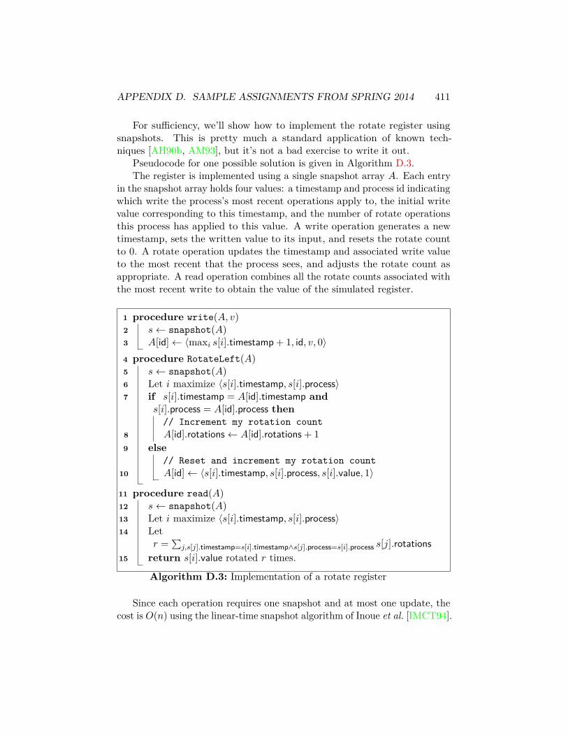
APPENDIX D. SAMPLE ASSIGNMENTS FROM SPRING 2014 411

For sufficiency, we’ll show how to implement the rotate register usingsnapshots. This is pretty much a standard application of known tech-niques [AH90b, AM93], but it’s not a bad exercise to write it out.

Pseudocode for one possible solution is given in Algorithm D.3.The register is implemented using a single snapshot array A. Each entry

in the snapshot array holds four values: a timestamp and process id indicatingwhich write the process’s most recent operations apply to, the initial writevalue corresponding to this timestamp, and the number of rotate operationsthis process has applied to this value. A write operation generates a newtimestamp, sets the written value to its input, and resets the rotate countto 0. A rotate operation updates the timestamp and associated write valueto the most recent that the process sees, and adjusts the rotate count asappropriate. A read operation combines all the rotate counts associated withthe most recent write to obtain the value of the simulated register.

1 procedure write(A, v)2 s← snapshot(A)3 A[id]← 〈maxi s[i].timestamp + 1, id, v, 0〉4 procedure RotateLeft(A)5 s← snapshot(A)6 Let i maximize 〈s[i].timestamp, s[i].process〉7 if s[i].timestamp = A[id].timestamp and

s[i].process = A[id].process then// Increment my rotation count

8 A[id].rotations← A[id].rotations + 19 else

// Reset and increment my rotation count10 A[id]← 〈s[i].timestamp, s[i].process, s[i].value, 1〉

11 procedure read(A)12 s← snapshot(A)13 Let i maximize 〈s[i].timestamp, s[i].process〉14 Let

r =∑j,s[j].timestamp=s[i].timestamp∧s[j].process=s[i].process s[j].rotations

15 return s[i].value rotated r times.

Algorithm D.3: Implementation of a rotate register

Since each operation requires one snapshot and at most one update, thecost is O(n) using the linear-time snapshot algorithm of Inoue et al. [IMCT94].

APPENDIX D. SAMPLE ASSIGNMENTS FROM SPRING 2014 412

Linearizability is easily verified by observing that ordering all operations bythe maximum timestamp/process tuple that they compute and then by thetotal number of rotations that they observe produces an ordering consistentwith the concurrent execution for which all return values of reads are correct.

D.6.2 A randomized two-process test-and-set

Algorithm D.4 gives pseudocode for a protocol for two processes p0 and p1.It uses two shared unbounded single-writer atomic registers r0 and r1, bothinitially 0. Each process also has a local variable s.

1 procedure TASi()2 while true do3 with probability 1/2 do4 ri ← ri + 15 else6 ri ← ri

7 s← r¬i8 if s > ri then9 return 1

10 else if s < ri − 1 do11 return 0

Algorithm D.4: Randomized two-process test-and-set for D.6.2

1. Show that any return values of the protocol are consistent with alinearizable, single-use test-and-set.

2. Will this protocol always terminate with probability 1 assuming anoblivious adversary?

3. Will this protocol always terminate with probability 1 assuming anadaptive adversary?

Solution

1. To show that this implements a linearizable test-and-set, we need toshow that exactly one process returns 0 and the other 1, and that if oneprocess finishes before the other starts, the first process to go returns1.

APPENDIX D. SAMPLE ASSIGNMENTS FROM SPRING 2014 413

Suppose that pi finishes before p¬i starts. Then pi reads only 0 fromr¬i, and cannot observe ri < r¬i: pi returns 0 in this case.We now show that the two processes cannot return the same value.Suppose that both processes terminate. Let i be such that pi reads r¬ifor the last time before p¬i reads ri for the last time. If pi returns 0,then it observes ri ≥ r¬i + 2 at the time of its read; p¬i can incrementr¬i at most once before reading ri again, and so observed r¬i < ri andreturns 1.Alternatively, if pi returns 1, it observed ri < r¬i. Since it performsno more increments on ri, pi also observes ri < r¬i in all subsequentreads, and so cannot also return 1.

2. Let’s run the protocol with an oblivious adversary, and track the valueof rt0 − rt1 over time, where rti is the value of ri after t writes (to eitherregister). Each write to r0 increases this value by 1/2 on average, witha change of 0 or 1 equally likely, and each write to r1 decreases it by1/2 on average.To make things look symmetric, let ∆t be the change caused by thet-th write and write ∆t as ct + Xt where ct = ±1/2 is a constantdetermined by whether p0 or p1 does the t-th write and Xt = ±1/2 isa random variable with expectation 0. Observe that the Xt variablesare independent of each other and the constants ct (which depend onlyon the schedule).For the protocol to run forever, at every time t it must hold that∣∣rt0 − rt1∣∣ ≤ 3; otherwise, even after one or both processes does itsnext write, we will have

∣∣∣rt′0 − rt′1 ∣∣∣ and the next process to read willterminate. But ∣∣∣rt0 − rt1∣∣∣ =

∣∣∣∣∣t∑

s=1∆s

∣∣∣∣∣=∣∣∣∣∣t∑

s=1(cs +Xs)

∣∣∣∣∣=∣∣∣∣∣t∑

s=1cs +

t∑s=1

Xs

∣∣∣∣∣.The left-hand sum is a constant, while the right-hand sum has abinomial distribution. For any fixed constant, the probability that abinomial distribution lands within ±2 of the constant goes to zero in

APPENDIX D. SAMPLE ASSIGNMENTS FROM SPRING 2014 414

the limit as t→∞, so with probability 1 there is some t for which thisevent does not occur.

3. For an adaptive adversary, the following strategy prevents agreement:

(a) Run p0 until it is about to increment r0.(b) Run p1 until it is about to increment r1.(c) Allow both increments to proceed and repeat.

The effect is that both processes always observe r0 = r1 wheneverthey do a read, and so never finish. This works because the adaptiveadversary can see the coin-flips done by the processes before they acton them; it would not work with an oblivious adversary or in a modelthat supported probabilistic writes.

D.7 CS465/CS565 Final Exam, May 2nd, 2014Write your answers in the blue book(s). Justify your answers. Work alone.Do not use any notes or books.

There are four problems on this exam, each worth 20 points, for a totalof 80 points. You have approximately three hours to complete this exam.

D.7.1 Maxima (20 points)

Some deterministic processes organized in an anonymous, synchronous ringare each given an integer input (which may or may not be distinct from otherprocesses’ inputs), but otherwise run the same code and do not know thesize of the ring. We would like the processes to each compute the maximuminput. As usual, each process may only return an output once, and must doso after a finite number of rounds, although it may continue to participatein the protocol (say, by relaying messages) even after it returns an output.

Prove or disprove: It is possible to solve this problem in this model.

Solution

It’s not possible.Consider an execution with n = 3 processes, each with input 0. If the

protocol is correct, then after some finite number of rounds t, each processreturns 0. By symmetry, the processes all have the same states and send thesame messages throughout this execution.

APPENDIX D. SAMPLE ASSIGNMENTS FROM SPRING 2014 415

Now consider a ring of size 2(t + 1) where every process has input 0,except for one process p that has input 1. Let q be the process at maximumdistance from p. By induction on r, we can show that after r rounds ofcommunication, every process that is more than r + 1 hops away from p hasthe same state as all of the processes in the 3-process execution above. So inparticular, after t rounds, process q (at distance t+ 1) is in the same stateas it would be in the 3-process execution, and thus it returns 0. But—as itlearns to its horror, one round too late—the correct maximum is 1.

D.7.2 Historyless objects (20 points)

Recall that a shared-memory object is historyless if any operation on theobject either (a) always leaves the object in the same state as before theoperation, or (b) always leaves the object in a new state that doesn’t dependon the state before the operation.

What is the maximum possible consensus number for a historyless object?That is, for what value n is it possible to solve wait-free consensus for nprocesses using some particular historyless object but not possible to solvewait-free consensus for n+ 1 processes using any historyless object?

Solution

Test-and-sets are (a) historyless, and (b) have consensus number 2, so n isat least 2.

To show that no historyless object can solve wait-free 3-process consensus,consider an execution that starts in a bivalent configuration and runs to aconfiguration C with two pending operations x and y such that Cx is 0-valentand Cy is 1-valent. By the usual arguments x and y must both be operationson the same object. If either of x and y is a read operation, then (0-valent)Cxy and (1-valent) Cyx are indistinguishable to a third process pz if runalone, because the object is left in the same state in both configurations;whichever way pz decides, it will give a contradiction in an execution startingwith one of these configurations. If neither of x and y is a read, then xoverwrites y, and Cx is indistinguishable from Cyxto pz if pz runs alone;again we get a contradiction.

D.7.3 Hams (20 points)

Hamazon, LLC, claims to be the world’s biggest delivery service for cannedhams, with guaranteed delivery of a canned ham to your home anywhereon Earth via suborbital trajectory from secret launch facilities at the North

APPENDIX D. SAMPLE ASSIGNMENTS FROM SPRING 2014 416

and South Poles. Unfortunately, these launch facilities may be subject tocrash failures due to inclement weather, trademark infringement actions, ormilitary retaliation for misdirected hams.

For this problem, you are to evaluate Hamazon’s business model fromthe perspective of distributed algorithms. Consider a system consisting ofa client process and two server processes (corresponding to the North andSouth Pole facilities) that communicate by means of asynchronous messagepassing. In addition to the usual message-passing actions, each server alsohas an irrevocable launch action that launches a ham at the client. As withmessages, hams are delivered asynchronously: it is impossible for the clientto tell if a ham has been launched until it arrives.

A ham protocol is correct provided (a) a client that orders no ham receivesno ham; and (b) a client that orders a ham receives exactly one ham. Showthat there can be no correct deterministic protocol for this problem if one ofthe servers can crash.

Solution

Consider an execution in which the client orders ham. Run the northernserver together with the client until the server is about to issue a launchaction (if it never does so, the client receives no ham when the southernserver is faulty).

Now run the client together with the southern server. There are twocases:

1. If the southern server ever issues launch, execute both this and thenorthern server’s launch actions: the client gets two hams.

2. If the southern server never issues launch, never run the northernserver again: the client gets no hams.

In either case, the one-ham rule is violated, and the protocol is notcorrect.5

5It’s tempting to try to solve this problem by reduction from a known impossibilityresult, like Two Generals or FLP. For these specific problems, direct reductions don’tappear to work. Two Generals assumes message loss, but in this model, messages are notlost. FLP needs any process to be able to fail, but in this model, the client never fails.Indeed, we can solve consensus in the Hamazon model by just having the client transmitits input to both servers.

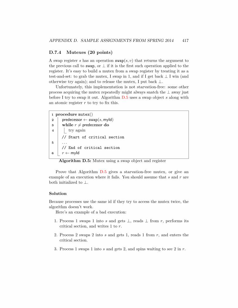
APPENDIX D. SAMPLE ASSIGNMENTS FROM SPRING 2014 417

D.7.4 Mutexes (20 points)

A swap register s has an operation swap(s, v) that returns the argument tothe previous call to swap, or ⊥ if it is the first such operation applied to theregister. It’s easy to build a mutex from a swap register by treating it as atest-and-set: to grab the mutex, I swap in 1, and if I get back ⊥ I win (andotherwise try again); and to release the mutex, I put back ⊥.

Unfortunately, this implementation is not starvation-free: some otherprocess acquiring the mutex repeatedly might always snatch the ⊥ away justbefore I try to swap it out. Algorithm D.5 uses a swap object s along withan atomic register r to try to fix this.

1 procedure mutex()2 predecessor← swap(s,myId)3 while r 6= predecessor do4 try again

// Start of critical section5 . . .

// End of critical section6 r ← myId

Algorithm D.5: Mutex using a swap object and register

Prove that Algorithm D.5 gives a starvation-free mutex, or give anexample of an execution where it fails. You should assume that s and r areboth initialized to ⊥.

Solution

Because processes use the same id if they try to access the mutex twice, thealgorithm doesn’t work.

Here’s an example of a bad execution:

1. Process 1 swaps 1 into s and gets ⊥, reads ⊥ from r, performs itscritical section, and writes 1 to r.

2. Process 2 swaps 2 into s and gets 1, reads 1 from r, and enters thecritical section.

3. Process 1 swaps 1 into s and gets 2, and spins waiting to see 2 in r.

APPENDIX D. SAMPLE ASSIGNMENTS FROM SPRING 2014 418

4. Process 3 swaps 3 into s and gets 1. Because r is still 1, process 3 readsthis 1 and enters the critical section. We now have two processes inthe critical section, violating mutual exclusion.

I believe this works if each process adopts a new id every time it callsmutex, but the proof is a little tricky.6

6The simplest proof I can come up with is to apply an invariant that says that (a)the processes that have executed swap(s,myId) but have not yet left the while loop havepredecessor values that form a linked list, with the last pointer either equal to ⊥ (if noprocess has yet entered the critical section) or the last process to enter the critical section;(b) r is ⊥ if no process has yet left the critical section, or the last process to leave thecritical section otherwise; and (c) if there is a process that is in the critical section, itspredecessor field points to the last process to leave the critical section. Checking the effectsof each operation shows that this invariant is preserved through the execution, and (a)combined with (c) show that we can’t have two processes in the critical section at the sametime. Additional work is still needed to show starvation-freedom. It’s a good thing thisalgorithm doesn’t work as written.

Appendix E

Sample assignments fromFall 2011

E.1 Assignment 1: due Wednesday, 2011-09-28, at17:00

Bureaucratic part

Send me email! My address is aspnes@cs.yale.edu.In your message, include:

1. Your name.

2. Your status: whether you are an undergraduate, grad student, auditor,etc.

3. Anything else you’d like to say.

(You will not be graded on the bureaucratic part, but you should do itanyway.)

E.1.1 Anonymous algorithms on a torus

An n × m torus is a two-dimensional version of a ring, where a node atposition (i, j) has a neighbor to the north at (i, j − 1), the east at (i+ 1, j),the south at (i, j + 1), and the west at (i− 1, j). These values wrap aroundmodulo n for the first coordinate and modulo m for the second; so (0, 0) hasneighbors (0,m− 1), (1, 0), (0, 1), and (n− 1, 0).

419

APPENDIX E. SAMPLE ASSIGNMENTS FROM FALL 2011 420

Suppose that we have a synchronous message-passing network in theform of an n×m torus, consisting of anonymous, identical processes that donot know n, m, or their own coordinates, but do have a sense of direction(meaning they can tell which of their neighbors is north, east, etc.).

Prove or disprove: Under these conditions, there is a deterministic1

algorithm that computes whether n > m.

Solution

Disproof: Consider two executions, one in an n ×m torus and one in anm× n torus where n > m and both n and m are at least 2.2 Using the sameargument as in Lemma 5.1.1, show by induction on the round number that,for each round r, all processes in both executions have the same state. Itfollows that if the processes correctly detect n > m in the n×m execution,then they incorrectly report m > n in the m× n execution.

E.1.2 Clustering

Suppose that k of the nodes in an asynchronous message-passing networkare designated as cluster heads, and we want to have each node learn theidentity of the nearest head. Given the most efficient algorithm you can forthis problem, and compute its worst-case time and message complexities.

You may assume that processes have unique identifiers and that allprocesses know how many neighbors they have.3

Solution

The simplest approach would be to run either of the efficient distributedbreadth-first search algorithms from Chapter 4 simultaneously starting at allcluster heads, and have each process learn the distance to all cluster headsat once and pick the nearest one. This gives O(D2) time and O(k(E + V D))messages if we use layering and O(D) time and O(kDE) messages usinglocal synchronization.

We can get rid of the dependence on k in the local-synchronizationalgorithm by running it almost unmodified, with the only difference beingthe attachment of a cluster head id to the exactly messages. The simplestway to show that the resulting algorithm works is to imagine coalescing

1Clarification added 2011-09-28.2This last assumption is not strictly necessary, but it avoids having to worry about

what it means when a process sends a message to itself.3Clarification added 2011-09-26.

APPENDIX E. SAMPLE ASSIGNMENTS FROM FALL 2011 421

all cluster heads into a single initiator; the clustering algorithm effectivelysimulates the original algorithm running in this modified graph, and thesame proof goes through. The running time is still O(D) and the messagecomplexity O(DE).

E.1.3 Negotiation

Two merchants A and B are colluding to fix the price of some valuablecommodity, by sending messages to each other for r rounds in a synchronousmessage-passing system. To avoid the attention of antitrust regulators, themerchants are transmitting their messages via carrier pigeons, which areunreliable and may become lost. Each merchant has an initial price pA orpB, which are integer values satisfying 0 ≤ p ≤ m for some known valuem, and their goal is to choose new prices p′A and p′B, where |p′A − p′B| ≤ 1.If pA = pB and no messages are lost, they want the stronger goal thatp′A = p′B = pA = pB.

Prove the best lower bound you can on r, as a function of m, for allprotocols that achieve these goals.

Solution

This is a thinly-disguised version of the Two Generals Problem from Chap-ter 8, with the agreement condition p′A = p′B replaced by an approximateagreement condition |p′A − p′B| ≤ 1. We can use a proof based on theindistinguishability argument in §8.2 to show that r ≥ m/2.

Fix r, and suppose that in a failure-free execution both processes sendmessages in all rounds (we can easily modify an algorithm that does nothave this property to have it, without increasing r). We will start with asequence of executions with pA = pB = 0. Let X0 be the execution in whichno messages are lost, X1 the execution in which A’s last message is lost,X2 the execution in which both A and B’s last messages are lost, and soon, with Xk for 0 ≤ k ≤ 2r losing k messages split evenly between the twoprocesses, breaking ties in favor of losing messages from A.

When i is even, Xi is indistinguishable from Xi+1 by A; it follows thatp′A is the same in both executions. Because we no longer have agreement,it may be that p′B(Xi) and p′B(Xi+1) are not the same as p′A in eitherexecution; but since both are within 1 of p′A, the difference between them isat most 2. Next, because Xi+1 to Xi+2 are indistinguishable to B, we havep′B(Xi+1) = p′B(Xi+2), which we can combine with the previous claim to get|p′B(Xi)− p′B(Xi+2)|. A simple induction then gives p′B(X2r) ≤ 2r, where

APPENDIX E. SAMPLE ASSIGNMENTS FROM FALL 2011 422

X2r is an execution in which all messages are lost.Now construct executions X2r+1 and X2r+2 by changing pA and pB to

m one at a time. Using essentially the same argument as before, we get|p′B(X2r)− p′B(X2r+2)| ≤ 2 and thus p′B(X2r+2) ≤ 2r + 2.

Repeat the initial 2r steps backward to get to an execution X4r+2 withpA = pB = m and no messages lost. Applying the same reasoning as aboveshows m = p′B(X4r+2) ≤ 4r + 2 or r ≥ m−2

4 = Ω(m).Though it is not needed for the solution, it is not too hard to unwind

the lower bound argument to extract an algorithm that matches the lowerbound up to a small constant factor. For simplicity, let’s assume m is even.

The protocol is to send my input in the first message and then use m/2−1subsequent acknowledgments, stopping immediately if I ever fail to receivea message in some round; the total number of rounds r is exactly m/2. IfI receive s messages in the first s rounds, I decide on min(pA, pB) if thatvalue lies in [m/2− s,m/2 + s] and the nearest endpoint otherwise. (Notethat if s = 0, I don’t need to compute min(pA, pB), and if s > 0, I can do sobecause I know both inputs.)

This satisfies the approximate agreement condition because if I see only smessages, you see at most s+1, because I stop sending once I miss a message.So either we both decide min(pA, pB) or we choose endpoints m/2 ± sAand m/2± sB that are within 1 of each other. It also satisfies the validitycondition p′A = p′B = pA = pB when both inputs are equal and no messagesare lost (and even the stronger requirement that p′A = p′B when no messagesare lost), because in this case [m/2− s,m/2 + s] is exactly [0,m] and bothprocesses decide min(pA, pB).

There is still a factor-of-2 gap between the upper and lower bounds. Myguess would be that the correct bound is very close to m/2 on both sides,and that my lower bound proof is not quite clever enough.

E.2 Assignment 2: due Wednesday, 2011-11-02, at17:00

E.2.1 Consensus with delivery notifications

The FLP bound (Chapter 11) shows that we can’t solve consensus in anasynchronous system with one crash failure. Part of the reason for this isthat only the recipient can detect when a message is delivered, so the otherprocesses can’t distinguish between a configuration in which a message hasor has not been delivered to a faulty process.

APPENDIX E. SAMPLE ASSIGNMENTS FROM FALL 2011 423

Suppose that we augment the system so that senders are notified imme-diately when their messages are delivered. We can model this by making thedelivery of a single message an event that updates the state of both senderand recipient, both of which may send additional messages in response. Letus suppose that this includes attempted deliveries to faulty processes, so thatany non-faulty process that sends a message m is eventually notified that mhas been delivered (although it might not have any effect on the recipient ifthe recipient has already crashed).

1. Show that this system can solve consensus with one faulty processwhen n = 2.

2. Show that this system cannot solve consensus with two faulty processeswhen n = 3.

Solution

1. To solve consensus, each process sends its input to the other. Whicheverinput is delivered first becomes the output value for both processes.

2. To show impossibility with n = 3 and two faults, run the usual FLPproof until we get to a configuration C with events e′ and e such thatCe is 0-valent and Ce′e is 1-valent (or vice versa). Observe that eand e′ may involve two processes each (sender and receiver), for upto four processes total, but only a process that is involved in both eand e′ can tell which happened first. There can be at most two suchprocesses. Kill both, and get that Ce′e is indistinguishable from Cee′

for the remaining process, giving the usual contradiction.

E.2.2 A circular failure detector

Suppose we equip processes 0 . . . n− 1 in an asynchronous message-passingsystem with n processes subject to crash failures with a failure detector thatis strongly accurate (no non-faulty process is ever suspected) and causesprocess i+ 1 (mod n) to eventually permanently suspect process i if processi crashes. Note that this failure detector is not even weakly complete (ifboth i and i+ 1 crash, no non-faulty process suspects i). Note also that thering structure of the failure detector doesn’t affect the actual network: eventhough only process i+ 1 (mod n) may suspect process i, any process cansend messages to any other process.

Prove the best upper and lower bounds you can on the largest number offailures f that allows solving consensus in this system.

APPENDIX E. SAMPLE ASSIGNMENTS FROM FALL 2011 424

Solution

There is an easy reduction to FLP that shows f ≤ n/2 is necessary (when nis even), and a harder reduction that shows f < 2

√n− 1 is necessary. The

easy reduction is based on crashing every other process; now no survivingprocess can suspect any other survivor, and we are back in an asynchronousmessage-passing system with no failure detector and 1 remaining failure (iff is at least n/2 + 1).

The harder reduction is to crash every (√n)-th process. This partitions

the ring into√n segments of length

√n− 1 each, where there is no failure

detector in any segment that suspects any process in another segment. If analgorithm exists that solves consensus in this situation, then it does so evenif (a) all processes in each segment have the same input, (b) if any process inone segment crashes, all

√n− 1 process in the segment crash, and (c) if any

process in a segment takes a step, all take a step, in some fixed order. Underthis additional conditions, each segment can be simulated by a single processin an asynchronous system with no failure detectors, and the extra

√n− 1

failures in 2√n− 1 correspond to one failure in the simulation. But we can’t

solve consensus in the simulating system (by FLP), so we can’t solve it inthe original system either.

On the other side, let’s first boost completeness of the failure detector,by having any process that suspects another transmit this submission byreliable broadcast. So now if any non-faulty process i suspects i+ 1, all thenon-faulty processes will suspect i+ 1. Now with up to t failures, wheneverI learn that process i is faulty (through a broadcast message passing on thesuspicion of the underlying failure detector, I will suspect processes i + 1through i + t − f as well, where f is the number of failures I have heardabout directly. I don’t need to suspect process i+ t− f + 1 (unless there issome intermediate process that has also failed), because the only way thatthis process will not be suspected eventually is if every process in the rangei to i+ t− f is faulty, which can’t happen given the bound t.

Now if t is small enough that I can’t cover the entire ring with thesesegments, then there is some non-faulty processes that is far enough awayfrom the nearest preceding faulty process that it is never suspected: this givesus an eventually strong failure detector, and we can solve consensus using thestandard Chandra-Toueg ♦S algorithm from §13.4 or [CT96]. The inequalityI am looking for is f(t− f) < n, where the left-hand side is maximized bysetting f = t/2, which gives t2/4 < n or t <

√2n. This leaves a gap of about√

2 between the upper and lower bounds; I don’t know which one can beimproved.

APPENDIX E. SAMPLE ASSIGNMENTS FROM FALL 2011 425

I am indebted to Hao Pan for suggesting the Θ(√n) upper and lower

bounds, which corrected an error in my original draft solution to this problem.

E.2.3 An odd problem

Suppose that each of n processes in a message-passing system with a completenetwork is attached to a sensor. Each sensor has two states, active andinactive; initially, all sensors are off. When the sensor changes state, thecorresponding process is notified immediately, and can update its stateand send messages to other processes in response to this event. It is alsoguaranteed that if a sensor changes state, it does not change state again forat least two time units. We would like to detect when an odd number ofsensors are active, by having at least one process update its state to set offan alarm at a time when this condition holds.

A correct protocol for this problem should satisfy two conditions:

No false positives If a process sets of an alarm, then an odd number ofsensors are active.

Termination If at some time an odd number of sensors are active, and fromthat point on no sensor changes its state, then some process eventuallysets off an alarm.

For what values of n is it possible to construct such a protocol?

Solution

It is feasible to solve the problem for n < 3.For n = 1, the unique process sets off its alarm as soon as its sensor

becomes active.For n = 2, have each process send a message to the other containing

its sensor state whenever the sensor state changes. Let s1 and s2 be thestate of the two process’s sensors, with 0 representing inactive and 1 active,and let pi set off its alarm if it receives a message s such that s ⊕ si = 1.This satisfies termination, because if we reach a configuration with an oddnumber of active sensors, the last sensor to change causes a message to besent to the other process that will cause it to set off its alarm. It satisfiesno-false-positives, because if pi sets off its alarm, then s¬i = s because atmost one time unit has elapsed since p¬i sent s; it follows that s¬i ⊕ si = 1and an odd number of sensors are active.

No such protocol is possible for n ≥ 3. Make p1’s sensor active. Run theprotocol until some process pi is about to enter an alarm state (this occurs

APPENDIX E. SAMPLE ASSIGNMENTS FROM FALL 2011 426

eventually because otherwise we violate termination). Let pj be one of p2or p3 with j 6= i, activate pj ’s sensor (we can do this without violating theonce-per-time-unit restriction because it has never previously been activated)and then let pi set off its alarm. We have now violated no-false-positives.

E.3 Assignment 3: due Friday, 2011-12-02, at 17:00

E.3.1 A restricted queue

Suppose you have an atomic queue Q that supports operations enq and deq,restricted so that:

• enq(Q) always pushes the identity of the current process onto the tailof the queue.

• deq(Q) tests if the queue is nonempty and its head is equal to theidentity of the current process. If so, it pops the head and returnstrue. If not, it does nothing and returns false.

The rationale for these restrictions is that this is the minimal version ofa queue needed to implement a starvation-free mutex using Algorithm 17.2.

What is the consensus number of this object?

Solution

The restricted queue has consensus number 1.Suppose we have 2 processes, and consider all pairs of operations on Q

that might get us out of a bivalent configuration C. Let x be an operationcarried out by p that leads to a b-valent state, and y an operation by q thatleads to a (¬b)-valent state. There are three cases:

• Two deq operations. If Q is empty, the operations commute. If thehead of the Q is p, then y is a no-op and p can’t distinguish betweenCx and Cyx. Similarly for q if the head is q.

• One enq and one deq operation. Suppose x is an enq and y a deq. IfQ is empty or the head is not q, then y is a no-op: p can’t distinguishCx from Cyx. If the head is q, then x and y commute. The same holdsin reverse if x is a deq and y an enq.

• Two enq operations. This is a little tricky, because Cxy and Cyx aredifferent states. However, if Q is nonempty in C, whichever process

APPENDIX E. SAMPLE ASSIGNMENTS FROM FALL 2011 427

isn’t at the head of Q can’t distinguish them, because any deq operationreturns false and never reaches the newly-enqueued values. This leavesthe case where Q is empty in C. Run p until it is poised to dox′ = deq(Q) (if this never happens, p can’t distinguish Cxy from Cyx);then run q until it is poised to do y′ = deq(Q) as well (same argumentas for p). Now allow both deq operations to proceed in whichever ordercauses them both to succeed. Since the processes can’t tell which deqhappened first, they can’t tell which enq happened first either. Slightlymore formally, if we let α be the sequence of operations leading up tothe two deq operations, we’ve just shown Cxyαx′y′ is indistinguishablefrom Cyxαy′x′ to both processes.

In all cases, we find that we can’t escape bivalence. It follows that Q can’tsolve 2-process consensus.

E.3.2 Writable fetch-and-increment

Suppose you are given an unlimited supply of atomic registers and fetch-and-increment objects, where the fetch-and-increment objects are all initialized to0 and supply only a fetch-and-increment operation that increments the objectand returns the old value. Show how to use these objects to construct a wait-free, linearizable implementation of an augmented fetch-and-increment thatalso supports a write operation that sets the value of the fetch-and-incrementand returns nothing.

Solution

We’ll use a snapshot object a to control access to an infinite array fof fetch-and-increments, where each time somebody writes to the imple-mented object, we switch to a new fetch-and-increment. Each cell in aholds (timestamp, base), where base is the starting value of the simulatedfetch-and-increment. We’ll also use an extra fetch-and-increment T to handout timestamps.

Code is in Algorithm E.1.Since this is all straight-line code, it’s trivially wait-free.Proof of linearizability is by grouping all operations by timestamp, us-

ing s[i].timestamp for FetchAndIncrement operations and t for write op-erations, then putting write before FetchAndIncrement, then orderingFetchAndIncrement by return value. Each group will consist of a write(v)for some v followed by zero or more FetchAndIncrement operations, whichwill return increasing values starting at v since they are just returning values

APPENDIX E. SAMPLE ASSIGNMENTS FROM FALL 2011 428

1 procedure FetchAndIncrement()2 s← snapshot(a)3 i← arg maxi(s[i].timestamp)4 return f [s[i].timestamp] + s[i].base

5 procedure write(v)6 t← FetchAndIncrement(T )7 a[myId]← (t, v)

Algorithm E.1: Resettable fetch-and-increment

from the underlying FetchAndIncrement object; the implementation thusmeets the specification.

To show consistency with the actual execution order, observe that time-stamps only increase over time and that the use of snapshot means thatany process that observes or writes a timestamp t does so at a time laterthan any process that observes or writes any t′ < t; this shows the grouporder is consistent. Within each group, the write writes a[myId] beforeany FetchAndIncrement reads it, so again we have consistency between thewrite and any FetchAndIncrement operations. The FetchAndIncrementoperations are linearized in the order in which they access the underlyingf [. . . ] object, so we win here too.

E.3.3 A box object

Suppose you want to implement an object representing a w × h box whosewidth (w) and height (h) can be increased if needed. Initially, the box is1× 1, and the coordinates can be increased by 1 each using IncWidth andIncHeight operations. There is also a GetArea operation that returns thearea w · h of the box.

Give an obstruction-free deterministic implementation of this object fromatomic registers that optimizes the worst-case individual step complexity ofGetArea, and show that your implementation is optimal by this measure upto constant factors.

Solution

Let b be the box object. Represent b by a snapshot object a, where a[i] holdsa pair (∆wi,∆hi) representing the number of times process i has executedIncWidth and IncHeight; these operations simply increment the appropriate

APPENDIX E. SAMPLE ASSIGNMENTS FROM FALL 2011 429

value and update the snapshot object. Let GetArea take a snapshot andreturn (

∑i ∆wi) (

∑i ∆hi); the cost of the snapshot is O(n).

To see that this is optimal, observe that we can use IncWidth and GetAreato represent inc and read for a standard counter. The Jayanti-Tan-Touegbound applies to counters, giving a worst-case cost of Ω(n) for GetArea.

E.4 CS465/CS565 Final Exam, December 12th, 2011Write your answers in the blue book(s). Justify your answers. Work alone.Do not use any notes or books.

There are four problems on this exam, each worth 20 points, for a totalof 80 points. You have approximately three hours to complete this exam.

General clarifications added during exam Assume all processes haveunique ids and know n. Assume that the network is complete in the message-passing model.

E.4.1 Lockable registers (20 points)

Most memory-management units provide the ability to control access tospecific memory pages, allowing a page to be marked (for example) read-only.Suppose that we model this by a lockable register that has the usualregister operations read(r) and write(r, v) plus an additional operationlock(r). The behavior of the register is just like a normal atomic registeruntil somebody calls lock(r); after this, any call to write(r) has no effect.

What is the consensus number of this object?

Solution

The consensus number is ∞; a single lockable register solves consensus forany number of processes. Code is in Algorithm E.2.

1 write(r, input)2 lock(r)3 return read(r)

Algorithm E.2: Consensus using a lockable register

Termination and validity are trivial. Agreement follows from the factthat whatever value is in r when lock(r) is first called will never change,and thus will be read and returned by all processes.

APPENDIX E. SAMPLE ASSIGNMENTS FROM FALL 2011 430

E.4.2 Byzantine timestamps (20 points)

Suppose you have an asynchronous message passing system with exactly oneByzantine process.

You would like the non-faulty processes to be able to acquire an increasingsequence of timestamps. A process should be able to execute the timestampprotocol as often as it likes, and it should be guaranteed that when a processis non-faulty, it eventually obtains a timestamp that is larger than anytimestamp returned in any execution of the protocol by a non-faulty processthat finishes before the current process’s execution started.

Note that there is no bound on the size of a timestamp, so having theByzantine process run up the timestamp values is not a problem, as long asit can’t cause the timestamps to go down.

For what values of n is it possible to solve this problem?

Solution

It is possible to solve the problem for all n except n = 3. For n = 1, there areno non-faulty processes, so the specification is satisfied trivially. For n = 2,there is only one non-faulty process: it can just keep its own counter andreturn an increasing sequence of timestamps without talking to the otherprocess at all.

For n = 3, it is not possible. Consider an execution in which messagesbetween non-faulty processes p and q are delayed indefinitely. If the Byzantineprocess r acts to each of p and q as it would if the other had crashed, thisexecution is indistinguishable to p and q from an execution in which r iscorrect and the other is faulty. Since there is no communication betweenp and q, it is easy to construct and execution in which the specification isviolated.

For n ≥ 4, the protocol given in Algorithm E.3 works.The idea is similar to the Attiya, Bar-Noy, Dolev distributed shared

memory algorithm [ABND95]. A process that needs a timestamp polls n− 1other processes for the maximum values they’ve seen and adds 1 to it; beforereturning, it sends the new timestamp to all other processes and waits toreceive n− 1 acknowledgments. The Byzantine process may choose not toanswer, but this is not enough to block completion of the protocol.

To show the timestamps are increasing, observe that after the completionof any call by i to getTimestamp, at least n− 2 non-faulty processes j havea value vj ≥ vi. Any call to getTimestamp that starts later sees at leastn− 3 > 0 of these values, and so computes a max that is at least as big as

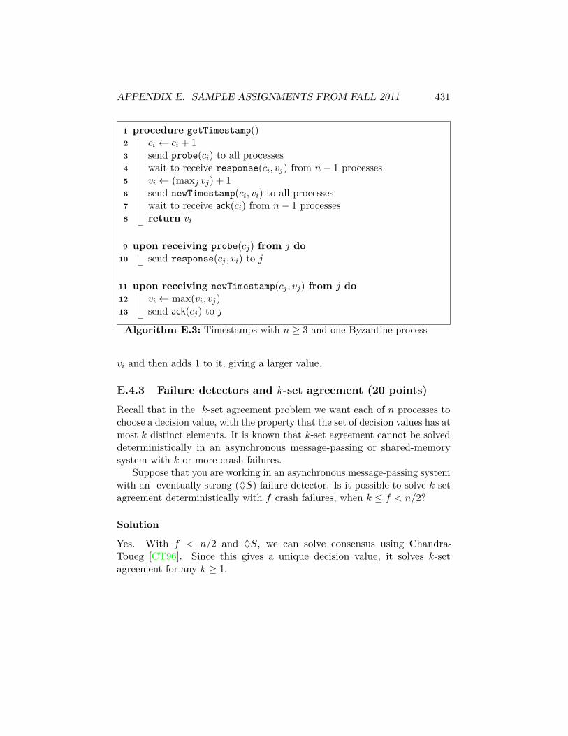
APPENDIX E. SAMPLE ASSIGNMENTS FROM FALL 2011 431

1 procedure getTimestamp()2 ci ← ci + 13 send probe(ci) to all processes4 wait to receive response(ci, vj) from n− 1 processes5 vi ← (maxj vj) + 16 send newTimestamp(ci, vi) to all processes7 wait to receive ack(ci) from n− 1 processes8 return vi

9 upon receiving probe(cj) from j do10 send response(cj , vi) to j

11 upon receiving newTimestamp(cj , vj) from j do12 vi ← max(vi, vj)13 send ack(cj) to j

Algorithm E.3: Timestamps with n ≥ 3 and one Byzantine process

vi and then adds 1 to it, giving a larger value.

E.4.3 Failure detectors and k-set agreement (20 points)

Recall that in the k-set agreement problem we want each of n processes tochoose a decision value, with the property that the set of decision values has atmost k distinct elements. It is known that k-set agreement cannot be solveddeterministically in an asynchronous message-passing or shared-memorysystem with k or more crash failures.

Suppose that you are working in an asynchronous message-passing systemwith an eventually strong (♦S) failure detector. Is it possible to solve k-setagreement deterministically with f crash failures, when k ≤ f < n/2?

Solution

Yes. With f < n/2 and ♦S, we can solve consensus using Chandra-Toueg [CT96]. Since this gives a unique decision value, it solves k-setagreement for any k ≥ 1.

APPENDIX E. SAMPLE ASSIGNMENTS FROM FALL 2011 432

E.4.4 A set data structure (20 points)

Consider a data structure that represents a set S, with an operation add(S, x)that adds x to S by setting S ← S ∪ x), and an operation size(S) thatreturns the number of distinct4 elements |S| of S. There are no restrictionson the types or sizes of elements that can be added to the set.

Show that any deterministic wait-free implementation of this object fromatomic registers has individual step complexity Ω(n) for some operation inthe worst case.

Solution

Algorithm E.4 implements a counter from a set object, where the counterread consists of a single call to size(S). The idea is that each increment isimplemented by inserting a new element into S, so |S| is always equal to thenumber of increments.

1 procedure inc(S)2 nonce← nonce + 13 add(S, 〈myId, nonce〉).

4 procedure read(S)5 return size(S)

Algorithm E.4: Counter from set object

Since the Jayanti-Tan-Toueg lower bound [JTT00] gives a lower boundof Ω(n) on the worst-case cost of a counter read, there exists an execution inwhich size(S) takes Ω(n) steps.

(We could also apply JTT directly by showing that the set object isperturbable; this follows because adding an element not added by anybodyelse is always visible to the reader.)

4Clarification added during exam.

Appendix F

Additional sample finalexams

This appendix contains final exams from previous times the course wasoffered, and is intended to give a rough guide to the typical format andcontent of a final exam. Note that the topics covered in past years were notnecessarily the same as those covered this year.

F.1 CS425/CS525 Final Exam, December 15th, 2005Write your answers in the blue book(s). Justify your answers. Work alone.Do not use any notes or books.

There are three problems on this exam, each worth 20 points, for a totalof 60 points. You have approximately three hours to complete this exam.

F.1.1 Consensus by attrition (20 points)

Suppose you are given a bounded fetch-and-subtract register that holdsa non-negative integer value and supports an operation fetch-and-subtract(k)for each k > 0 that (a) sets the value of the register to the previous valueminus k, or zero if this result would be negative, and (b) returns the previousvalue of the register.

Determine the consensus number of bounded fetch-and-subtract underthe assumptions that you can use arbitrarily many such objects, that you cansupplement them with arbitrarily many multiwriter/multireader read/writeregisters, that you can initialize all registers of both types to initial values of

433

APPENDIX F. ADDITIONAL SAMPLE FINAL EXAMS 434

your choosing, and that the design of the consensus protocol can depend onthe number of processes N .

Solution

The consensus number is 2.To implement 2-process wait-free consensus, use a single fetch-and-

subtract register initialized to 1 plus two auxiliary read/write registersto hold the input values of the processes. Each process writes its input to itsown register, then performs a fetch-and-subtract(1) on the fetch-and-subtractregister. Whichever process gets 1 from the fetch-and-subtract returns itsown input; the other process (which gets 0) returns the winning process’sinput (which it can read from the winning process’s read/write register.)

To show that the consensus number is at most 2, observe that any twofetch-and-subtract operations commute: starting from state x, after fetch-and-subtract(k1) and fetch-and-subtract(k2) the value in the fetch-and-subtractregister is max(0, x− k1 − k2) regardless of the order of the operations.

F.1.2 Long-distance agreement (20 points)

Consider an asynchronous message-passing model consisting of N processesp1 . . . pN arranged in a line, so that each process i can send messages only toprocesses i− 1 and i+ 1 (if they exist). Assume that there are no failures,that local computation takes zero time, and that every message is deliveredat most 1 time unit after it is sent no matter how many messages are senton the same edge.

Now suppose that we wish to solve agreement in this model, wherethe agreement protocol is triggered by a local input event at one or moreprocesses and it terminates when every process executes a local decide event.As with all agreement problems, we want Agreement (all processes decidethe same value), Termination (all processes eventually decide), and Validity(the common decision value previously appeared in some input). We alsowant no false starts: the first action of any process should either be an inputaction or the receipt of a message.

Define the time cost of a protocol for this problem as the worst-casetime between the first input event and the last decide event. Give the bestupper and lower bounds you can on this time as function of N . Your upperand lower bounds should be exact: using no asymptotic notation or hiddenconstant factors. Ideally, they should also be equal.

APPENDIX F. ADDITIONAL SAMPLE FINAL EXAMS 435

Solution

Upper bound

Because there are no failures, we can appoint a leader and have it decide.The natural choice is some process near the middle, say pb(N+1)/2c. Uponreceiving an input, either directly through an input event or indirectly fromanother process, the process sends the input value along the line toward theleader. The leader takes the first input it receives and broadcasts it back outin both directions as the decision value. The worst case is when the protocolis initiated at pN ; then we pay 2(N −b(N + 1)/2c) time to send all messagesout and back, which is N time units when N is even and N − 1 time unitswhen N is odd.

Lower bound

Proving an almost-matching lower bound of N − 1 time units is trivial: ifp1 is the only initiator and it starts at time t0, then by an easy inductionargument,in the worst case pi doesn’t learn of any input until time t0 +(i−1),and in particular pN doesn’t find out until after N − 1 time units. If pNnonetheless decides early, its decision value will violate validity in someexecutions.

But we can actually prove something stronger than this: that N timeunits are indeed required when N is odd. Consider two slow executions Ξ0and Ξ1, where (a) all messages are delivered after exactly one time unit ineach execution; (b) in Ξ0 only p1 receives an input and the input is 0; and (c)in Ξ1 only pN receives an input and the input is 1. For each of the executions,construct a causal ordering on events in the usual fashion: a send is orderedbefore a receive, two events of the same process are ordered by time, andother events are partially ordered by the transitive closure of this relation.

Now consider for Ξ0 the set of all events that precede the decide(0) eventof p1 and for Ξ1 the set of all events that precede the decide(1) event ofpN . Consider further the sets of processes S0 and S1 at which these eventsoccur; if these two sets of processes do not overlap, then we can constructan execution in which both sets of events occur, violating Agreement.

Because S0 and S1 overlap, we must have |S0| + |S1| ≥ N + 1, and soat least one of the two sets has size at least d(N + 1)/2e, which is N/2 + 1when N is even. Suppose that it is S0. Then in order for any event to occurat pN/2+1 at all some sequence of messages must travel from the initial inputto p1 to process pN/2+1 (taking N/2 time units), and the causal orderingimplies that an additional sequence of messages travels back from pN/2+1 to

APPENDIX F. ADDITIONAL SAMPLE FINAL EXAMS 436

p1 before p1 decides (taking and additional N/2 time units). The total timeis thus N .

F.1.3 Mutex appendages (20 points)

An append register supports standard read operations plus an appendoperation that appends its argument to the list of values already in theregister. An append-and-fetch register is similar to an append register,except that it returns the value in the register after performing the appendoperation. Suppose that you have an failure-free asynchronous system withanonymous deterministic processes (i.e., deterministic processes that all runexactly the same code). Prove or disprove each of the following statements:

1. It is possible to solve mutual exclusion using only append registers.

2. It is possible to solve mutual exclusion using only append-and-fetchregisters.

In either case, the solution should work for arbitrarily many processes—solvingmutual exclusion when N = 1 is not interesting. You are also not requiredin either case to guarantee lockout-freedom.

Clarification given during exam

1. If it helps, you may assume that the processes know N . (It probablydoesn’t help.)

Solution

1. Disproof: With append registers only, it is not possible to solve mutualexclusion. To prove this, construct a failure-free execution in whichthe processes never break symmetry. In the initial configuration, allprocesses have the same state and thus execute either the same readoperation or the same append operation; in either case we let all Noperations occur in some arbitrary order. If the operations are allreads, all processes read the same value and move to the same newstate. If the operations are all appends, then no values are returned andagain all processes enter the same new state. (It’s also the case thatthe processes can’t tell from the register’s state which of the identicalappend operations went first, but we don’t actually need to use thisfact.)

APPENDIX F. ADDITIONAL SAMPLE FINAL EXAMS 437

Since we get a fair failure-free execution where all processes movethrough the same sequence of states, if any process decides it’s in itscritical section, all do. We thus can’t solve mutual exclusion in thismodel.

2. Since the processes are anonymous, any solution that depends on themhaving identifiers isn’t going to work. But there is a simple solutionthat requires only appending single bits to the register.Each process trying to enter a critical section repeatedly executes anappend-and-fetch operation with argument 0; if the append-and-fetchoperation returns either a list consisting only of a single 0 or a listwhose second-to-last element is 1, the process enters its critical section.To leave the critical section, the process does append-and-fetch(1).

F.2 CS425/CS525 Final Exam, May 8th, 2008Write your answers in the blue book(s). Justify your answers. Work alone.Do not use any notes or books.

There are four problems on this exam, each worth 20 points, for a totalof 80 points. You have approximately three hours to complete this exam.

F.2.1 Message passing without failures (20 points)

Suppose you have an asynchronous message-passing system with a completecommunication graph, unique node identities, and no failures. Show that anydeterministic atomic shared-memory object can be simulated in this model,or give an example of a shared-memory object that can’t be simulated.

Solution

Pick some leader node to implement the object. To execute an operation,send the operation to the leader node, then have the leader carry out theoperation (sequentially) on its copy of the object and send the results back.

F.2.2 A ring buffer (20 points)

Suppose you are given a ring buffer object that consists of k ≥ 1 memorylocations a[0] . . . a[k − 1] with an atomic shift-and-fetch operation that takesan argument v and (a) shifts v into the buffer, so that a[i] ← a[i + 1] for

APPENDIX F. ADDITIONAL SAMPLE FINAL EXAMS 438

each i less than k − 1 and a[k − 1]← v; and (b) returns a snapshot of thenew contents of the array (after the shift).

What is the consensus number of this object as a function of k?

Solution

We can clearly solve consensus for at least k processes: each process callsshift-and-fetch on its input, and returns the first non-null value in the buffer.

So now we want to show that we can’t solve consensus for k+ 1 processes.Apply the usual FLP-style argument to get to a bivalent configuration Cwhere each of the k + 1 processes has a pending operation that leads to aunivalent configuration. Let e0 and e1 be particular operations leading to0-valent and 1-valent configurations, respectively, and let e2 . . . ek be theremaining k − 1 pending operations.

We need to argue first that no two distinct operations ei and ej areoperations of different objects. Suppose that Cei is 0-valent and Cej is1-valent; then if ei and ej are on different objects, Ceiej (still 0-valent) isindistinguishable by all processes from Cejei (still 1-valent), a contradiction.Alternatively, if ei and ej are both b-valent, there exists some (1−b)-valent eksuch that ei and ej both operate on the same object as ek, by the precedingargument. So all of e0 . . . ek are operations on the same object.

By the usual argument we know that this object can’t be a register. Let’sshow it can’t be a ring buffer either. Consider the configurations Ce0e1 . . . ekand Ce1 . . . ek. These are indistinguishable to the process carrying out ek(because its sees only the inputs to e1 through ek in its snapshot). So theymust have the same valence, a contradiction.

It follows that the consensus number of a k-element ring buffer is exactlyk.

F.2.3 Leader election on a torus (20 points)

An n × n torus is a graph consisting of n2 nodes, where each node (i, j),0 ≤ i, j ≤ n − 1, is connected to nodes (i − 1, j), (i + 1, j), (i, j − 1), and(i, j + 1), where all computation is done mod n.

Suppose you have an asynchronous message-passing system with a com-munication graph in the form of an n× n torus. Suppose further that eachnode has a unique identifier (some large natural number) but doesn’t knowthe value of n. Give an algorithm for leader election in this model with thebest message complexity you can come up with.

APPENDIX F. ADDITIONAL SAMPLE FINAL EXAMS 439

Solution

First observe that each row and column of the torus is a bidirectional ring, sowe can run e.g. Hirschbirg and Sinclair’s O(n logn)-message protocol withineach of these rings to find the smallest identifier in the ring. We’ll use thisto construct the following algorithm:

1. Run Hirschbirg-Sinclair in each row to get a local leader for each row;this takes n×O(n logn) = O(n2 logn) messages. Use an additional nmessages per row to distribute the identifier for the row leader to allnodes and initiate the next stage of the protocol.

2. Run Hirschbirg-Sinclair in each column with each node adopting the rowleader identifier as its own. This costs another O(n2 logn) messages;at the end, every node knows the minimum identifier of all nodes inthe torus.

The total message complexity is O(n2 logn). (I suspect this is optimal,but I don’t have a proof.)

F.2.4 An overlay network (20 points)

A collection of n nodes—in an asynchronous message-passing system with aconnected, bidirectional communications graph withO(1) links per node—wishto engage in some strictly legitimate file-sharing. Each node starts with someinput pair (k, v), where k is a key and v is a value, and the search problemis to find the value v corresponding to a particular key k.

1. Suppose that we can’t do any preparation ahead of time. Give analgorithm for searching with the smallest asymptotic worst-case messagecomplexity you can find as a function of n. You may assume that thereare no limits on time complexity, message size, or storage space at eachnode.

2. Suppose now that some designated leader node can initiate a protocolahead of time to pre-process the data in the nodes before any query isinitiated. Give a pre-processing algorithm (that does not depend onwhich key is eventually searched for) and associated search algorithmsuch that the search algorithm minimizes the asymptotic worst-casemessage complexity. Here you may assume that there are no limits ontime complexity, message size, or storage space for either algorithm, andthat you don’t care about the message complexity of the pre-processingalgorithm.

APPENDIX F. ADDITIONAL SAMPLE FINAL EXAMS 440

3. Give the best lower bound you can on the total message complexity ofthe pre-processing and search algorithms in the case above.

Solution

1. Run depth-first search to find the matching key and return the corre-sponding value back up the tree. Message complexity is O(|E|) = O(n)(since each node has only O(1) links).

2. Basic idea: give each node a copy of all key-value pairs, then searchestake zero messages. To give each node a copy of all key-value pairs wecould do convergecast followed by broadcast (O(n) message complexity)or just flood each pair O(n2). Either is fine since we don’t care aboutthe message complexity of the pre-processing stage.

3. Suppose the total message complexity of both the pre-processing stageand the search protocol is less than n − 1. Then there is some nodeother than the initiator of the search that sends no messages at anytime during the protocol. If this is the node with the matching key-value pair, we don’t find it. It follows that any solution to the searchproblem. requires a total of Ω(n) messages in the pre-processing andsearch protocols.

F.3 CS425/CS525 Final Exam, May 10th, 2010Write your answers in the blue book(s). Justify your answers. Work alone.Do not use any notes or books.

There are four problems on this exam, each worth 20 points, for a totalof 80 points. You have approximately three hours to complete this exam.

F.3.1 Anti-consensus (20 points)

A wait-free anti-consensus protocol satisfies the conditions:

Wait-free termination Every process decides in a bounded number of itsown steps.

Non-triviality There is at least one process that decides different valuesin different executions.

Disagreement If at least two processes decide, then some processes decideon different values.

APPENDIX F. ADDITIONAL SAMPLE FINAL EXAMS 441

Show that there is no deterministic wait-free anti-consensus protocolusing only atomic registers for two processes and two possible output values,but there is one for three processes and three possible output values.

Clarification: You should assume processes have distinct identities.

Solution

No protocol for two: turn an anti-consensus protocol with outputs in 0, 1into a consensus protocol by having one of the processes always negate itsoutput.

A protocol for three: Use a splitter.

F.3.2 Odd or even (20 points)

Suppose you have a protocol for a synchronous message-passing ring that isanonymous (all processes run the same code) and uniform (this code is thesame for rings of different sizes). Suppose also that the processes are giveninputs marking some, but not all, of them as leaders. Give an algorithmfor determining if the size of the ring is odd or even, or show that no suchalgorithm is possible.

Clarification: Assume a bidirectional, oriented ring and a deterministicalgorithm.

Solution

Here is an impossibility proof. Suppose there is such an algorithm, and letit correctly decide “odd” on a ring of size 2k + 1 for some k and some setof leader inputs. Now construct a ring of size 4k + 2 by pasting two suchrings together (assigning the same values to the leader bits in each copy)and run the algorithm on this ring. By the usual symmetry argument, everycorresponding process sends the same messages and makes the same decisionsin both rings, implying that the processes incorrectly decide the ring of size4k + 2 is odd.

F.3.3 Atomic snapshot arrays using message-passing (20 points)

Consider the following variant of Attiya-Bar-Noy-Dolev for obtaining snap-shots of an array instead of individual register values, in an asynchronousmessage-passing system with t < n/4 crash failures. The data structure we

APPENDIX F. ADDITIONAL SAMPLE FINAL EXAMS 442

are simulating is an array a consisting of an atomic register a[i] for eachprocess i, with the ability to perform atomic snapshots.

Values are written by sending a set of 〈i, v, ti〉 values to all processes,where i specifies the segment a[i] of the array to write, v gives a value forthis segment, and ti is an increasing timestamp used to indicate more recentvalues. We use a set of values because (as in ABD) some values may beobtained indirectly.

To update segment a[i] with value v, process i generates a new timestampti, sends 〈i, v, ti〉 to all processes, and waits for acknowledgments from atleast 3n/4 processes.

Upon receiving a message containing one or more 〈i, v, ti〉 triples, a processupdates its copy of a[i] for any i with a higher timestamp than previouslyseen, and responds with an acknowledgment (we’ll assume use of nonces sothat it’s unambiguous which message is being acknowledged).

To perform a snapshot, a process sends snapshot to all processes, andwaits to receive responses from at least 3n/4 processes, which will consist ofthe most recent values of each a[i] known by each of these processes togetherwith their timestamps (it’s a set of triples as above). The snapshot processthen takes the most recent versions of a[i] for each of these responses andupdates its own copy, then sends its entire snapshot vector to all processesand waits to receive at least 3n/4 acknowledgments. When it has receivedthese acknowledgments, it returns its own copy of a[i] for all i.

Prove or disprove: The above procedure implements an atomic snapshotarray in an asynchronous message-passing system with t < n/4 crash failures.

Solution

Disproof: Let s1 and s2 be processes carrying out snapshots and let w1 andw2 be processes carrying out writes. Suppose that each wi initiates a writeof 1 to a[wi], but all of its messages to other processes are delayed after itupdates its own copy awi [wi]. Now let each si receive responses from 3n/4−1processes not otherwise mentioned plus wi. Then s1 will return a vectorwith a[w1] = 1 and a[w2] = 0 while s2 will return a vector with a[w1] = 0and a[w2] = 1, which is inconsistent. The fact that these vectors are alsodisseminated throughout at least 3n/4 other processes is a red herring.

F.3.4 Priority queues (20 points)

Let Q be a priority queue whose states are multisets of natural numbers andthat has operations enq(v) and deq(), where enq(p) adds a new value v to

APPENDIX F. ADDITIONAL SAMPLE FINAL EXAMS 443

the queue, and deq() removes and returns the smallest value in the queue,or returns null if the queue is empty. (If there is more than one copy of thesmallest value, only one copy is removed.)

What is the consensus number of this object?

Solution

The consensus number is 2. The proof is similar to that for a queue.To show we can do consensus for n = 2, start with a priority queue with

a single value in it, and have each process attempt to dequeue this value. Ifa process gets the value, it decides on its own input; if it gets null, it decideson the other process’s input.

To show we can’t do consensus for n = 3, observe first that starting fromany states C of the queue, given any two operations x and y that are bothenqueues or both dequeues, the states Cxy and Cyx are identical. Thismeans that a third process can’t tell which operation went first, meaningthat a pair of enqueues or a pair of dequeues can’t get us out of a bivalentconfiguration in the FLP argument. We can also exclude any split involvingtwo operations on different queues (or other objects) But we still need toconsider the case of a dequeue operation d and an enqueue operation e onthe same queue Q. This splits into several subcases, depending on the stateC of the queue in some bivalent configuration:

1. C = . Then Ced = Cd = , and a third process can’t tell which ofd or e went first.

2. C is nonempty and e = enq(v), where v is greater than or equal to thesmallest value in C. Then Cde and Ced are identical, and no thirdprocess can tell which of d or e went first.

3. C is nonempty and e = enq(v), where v is less than any value in C.Consider the configurations Ced and Cde. Here the process pd thatperforms d can tell which operation went first, because it either obtainsv or some other value v′ 6= v. Kill this process. No other process in Cedor Cde can distinguish the two states without dequeuing whichever ofv or v′ was not dequeued by pd. So consider two parallel executionsCedσ and Cdeσ where σ consists of an arbitrary sequence of operationsending with a deq on Q by some process p (if no process ever attemptsto dequeue from Q, then we have already won, since the survivors can’tdistinguish Ced from Cde). Now the state of all objects is the sameafter Cedσ and Cdeσ, and only pd and p have different states in thesetwo configurations. So any third process is out of luck.

Appendix G

I/O automata

G.1 Low-level view: I/O automataAn I/O automaton [LT87] is an automaton where transitions are labeledby actions, which come in three classes: input actions, triggered by theoutside world; output actions triggered by the automaton and visibleto the outside world; and internal actions, triggered by the automatonbut not visible to the outside world. These classes correspond to inputs,outputs, and internal computation steps of the automaton; the latter areprovided mostly to give merged input/output actions a place to go whenautomata are composed together. A transition relation trans(A) relatesstates(A)× acts(A)× states(A); if (s, a, s′) is in trans(A), it means thatA can move from state s to state s′ by executing action a.

There is also an equivalence relation task(A) on the output and internalactions, which is used for enforcing fairness conditions—the basic idea is thatin a fair execution some action in each equivalence class must be executedeventually (a more accurate definition will be given below).

The I/O automaton model carries with it a lot of specialized jargon.We’ll try to avoid it as much as possible. One thing that will be difficult toavoid in reading [Lyn96] is the notion of a signature, which is just the tuplesig(A) = (in(A), out(A), int(A)) describing the actions of an automatonA.

G.1.1 Enabled actions

An action a is enabled in some state s if trans(A) contains at least onetransition (s, a, s′). Input actions are always enabled—this is a requirement ofthe model. Output and internal actions—the “locally controlled” actions—are

444

APPENDIX G. I/O AUTOMATA 445

not subject to this restriction. A state s is quiescent if only input actionsare enabled in s.

G.1.2 Executions, fairness, and traces

An execution of A is a sequence s0a0s1a1 . . . where each triple (si, aisi+1)is in trans(A). Executions may be finite or infinite; if finite, they must endin a state.

A trace of A is a subsequence of some execution consisting preciselyof the external (i.e., input and output) actions, with states and internalactions omitted. If we don’t want to get into the guts of a particularI/O automaton—and we usually don’t, unless we can’t help it because wehave to think explicitly about states for some reason—we can describe itsexternally-visible behavior by just giving its set of traces.

G.1.3 Composition of automata

Composing a set of I/O automata yields a new super-automaton whose stateset is the Cartesian product of the state sets of its components and whoseaction set is the union of the action sets of its components. A transitionwith a given action a updates the states of all components that have a as anaction and has no effect on the states of other components. The classificationof actions into the three classes is used to enforce some simple compatibilityrules on the component automata; in particular:

1. An internal action of a component is never an action of another com-ponent—internal actions are completely invisible.

2. No output action of a component can be an output action of anothercomponent.

3. No action is shared by infinitely many components.1 In practicethis means that no action can be an input action of infinitely manycomponents, since the preceding rules mean that any action is anoutput or internal action of at most one component.

All output actions of the components are also output actions of thecomposition. An input action of a component is an input of the compositiononly if some other component doesn’t supply it as an output; in this case

1Note that infinite (but countable) compositions are permitted.

APPENDIX G. I/O AUTOMATA 446

it becomes an output action of the composition. Internal actions remaininternal (and largely useless, except for bookkeeping purposes).

The task equivalence relation is the union of the task relations for thecomponents: this turns out to give a genuine equivalence relation on outputand internal actions precisely because the first two compatibility rules hold.

Given an execution or trace X of a composite automaton that includesA, we can construct the corresponding execution or trace X|A of A whichjust includes the states of A and the actions visible to A (events that don’tchange the state of A drop out). The definition of composition is chosen sothat X|A is in fact an execution/trace of A whenever X is.

G.1.4 Hiding actions

Composing A and B continues to expose the outputs of A even if they lineup with inputs of B. While this may sometimes be desirable, often we wantto shove such internal communication under the rug. The model lets us dothis by redefining the signature of an automaton to make some or all of theoutput actions into internal actions.

G.1.5 Fairness

I/O automata come with a built-in definition of fair executions, where anexecution of A is fair if, for each equivalence class C of actions in task(A),

1. the execution is finite and no action in C is enabled in the final state,or

2. the execution is infinite and there are infinitely many occurrences ofactions in C, or

3. the execution is infinite and there are infinitely many states in whichno action in C is enabled.

If we think of C as corresponding to some thread or process, this saysthat C gets infinitely many chances to do something in an infinite execution,but may not actually do them if it gives ups and stops waiting (the thirdcase). The finite case essentially says that a finite execution isn’t fair unlessnobody is waiting at the end. The motivation for this particular definitionis that it guarantees (a) that any finite execution can be extended to a fairexecution and (b) that the restriction X|A of a fair execution or trace X isalso fair.

APPENDIX G. I/O AUTOMATA 447

Fairness is useful e.g. for guaranteeing message delivery in a message-passing system: make each message-delivery action its own task class and eachmessage will eventually be delivered; similarly make each message-sendingaction its own task class and a process will eventually send every messageit intends to send. Tweaking the task classes can allow for possibilities ofstarvation, e.g. if all message-delivery actions are equivalent then a spammercan shut down the system in a “fair” execution where only his (infinitelymany) messages are delivered.

G.1.6 Specifying an automaton

The typical approach is to write down preconditions and effects for eachaction (for input actions, the preconditions are empty). An example wouldbe the spambot in Algorithm G.1.

1 input action setMessage(m)2 effects3 state← m

4 output action spam(m)5 precondition6 spam = m

7 effects8 none (keep spamming)

Algorithm G.1: Spambot as an I/O automaton

(Plus an initial state, e.g. state = ⊥, where ⊥ is not a possible message,and a task partition, of which we will speak more below when we talk aboutliveness properties.)

G.2 High-level view: tracesWhen studying the behavior of a system, traces are what we really careabout, and we want to avoid talking about states as much as possible. Sowhat we’ll aim to do is to get rid of the states early by computing the setof traces (or fair traces) of each automaton in our system, then composetraces to get traces for the system as a whole. Our typical goal will be toshow that the resulting set of traces has some desirable properties, usuallyof the form (1) nothing bad happens (a safety property); (2) something

APPENDIX G. I/O AUTOMATA 448

good eventually happens (a liveness property); or (3) the horribly complexcomposite automaton representing this concrete system acts just like thatnice clean automaton representing a specification (a simulation).

Very formally, a trace property specifies both the signature of theautomaton and a set of traces, such that all traces (or perhaps fair traces) ofthe automata appear in the set. We’ll usually forget about the first part.

Tricky detail: It’s OK if not all traces in P are generated by A (we wanttrace(A) ⊆ P , but not necessarily trace(A) = P ). But trace(A) will bepretty big (it includes, for example, all finite sequences of input actions)so hopefully the fact that A has to do something with inputs will tell ussomething useful.

G.2.1 Example

A property we might demand of the spambot above (or some other abstractionof a message channel) is that it only delivers messages that have previouslybeen given to it. As a trace property this says that in any trace t, iftk = spam(m), then tj = setMessage(m) for some j < k. (As a set, thisis just the set of all sequences of external spambot-actions that have thisproperty.) Call this property P .

To prove that the spambot automaton given above satisfies P , we mightargue that for any execution s0a0s1a1 . . . , that si = m in the last setMessageaction preceding si, or ⊥ if there is no such action. This is easily provedby induction on i. It then follows that since spam(m) can only transmit thecurrent state, that if spam(m) follows si = m that it follows some earliersetMessage(m) as claimed.

However, there are traces that satisfy P that don’t correspond to execu-tions of the spambot; for example, consider the trace setMessage(0)setMessage(1)spam(0).This satisfies P (0 was previously given to the automaton spam(0)), butthe automaton won’t generate it because the 0 was overwritten by the latersetMessage(1) action. Whether this is indicates a problem with our automa-ton not being nondeterministic enough or our trace property being too weakis a question about what we really want the automaton to do.

G.2.2 Types of trace properties

G.2.2.1 Safety properties

P is a safety property if

1. P is nonempty.

APPENDIX G. I/O AUTOMATA 449

2. P is prefix-closed, i.e. if xy is in P then x is in P .

3. P is limit-closed, i.e. if x1, x1x2, x1x2x3, . . . are all in P , then so isthe infinite sequence obtained by taking their limit.

Because of the last restrictions, it’s enough to prove that P holds for allfinite traces of A to show that it holds for all traces (and thus for all fairtraces), since any trace is a limit of finite traces. Conversely, if there is sometrace or fair trace for which P fails, the second restriction says that P failson any finite prefix of P , so again looking at only finite prefixes is enough.The spambot property mentioned above is a safety property.

Safety properties are typically proved using invariants, properties thatare shown by induction to hold in all reachable states.

G.2.2.2 Liveness properties

P is a liveness property of A if any finite sequence of actions in acts(A)has an extension in P . Note that liveness properties will in general includemany sequences of actions that aren’t traces of A, since they are extensionsof finite sequences that A can’t do (e.g. starting the execution with an actionnot enabled in the initial state). If you want to restrict yourself only toproper executions of A, use a safety property. (It’s worth noting that thesame property P can’t do both: any P that is both a liveness and a safetyproperty includes all sequences of actions because of the closure rules.)

Liveness properties are those that are always eventually satisfiable; as-serting one says that the property is eventually satisfied. The typical wayto prove a liveness property is with a progress function, a function fon states that (a) drops by at least 1 every time something that happensinfinitely often happens (like an action from an always-enabled task class)and (b) guarantees P once it reaches 0.

An example would be the following property we might demand of ourspambot: any trace with at least one setMessage(. . . ) action contains infinitelymany spam(. . . ) actions. Whether the spambot automaton will satisfy thisproperty (in fair traces) depends on its task partition. If all spam(. . . ) actionsare in the same equivalence class, then any execution with at least one setMes-sage will have some spam (. . . ) action enabled at all times thereafter, so a fairtrace containing a setMessage can’t be finite (since spam is enabled in the laststate) and if infinite contains infinitely many spam messages (since spam mes-sages of some sort are enabled in all but an initial finite prefix). On the otherhand, if spam(m1) and spam(m2) are not equivalent in task(A), then thespambot doesn’t satisfy the liveness property: in an execution that alternates

APPENDIX G. I/O AUTOMATA 450

setMessage(m1)setMessage(m2)setMessage(m1)setMessage(m2) . . . there areinfinitely many states in which spam(m1) is not enabled, so fairness doesn’trequire doing it even once, and similarly for spam(m2).

G.2.2.3 Other properties

Any other property P can be expressed as the intersection of a safety property(the closure of P ) and a liveness property (the union of P and the set of allfinite sequences that aren’t prefixes of traces in P ). The intuition is thatthe safety property prunes out the excess junk we threw into the livenessproperty to make it a liveness property, since any sequence that isn’t a prefixof a trace in P won’t go into the safety property. This leaves only the tracesin P .

Example: Let P = 0n1∞ be the set of traces where we eventually giveup on our pointless 0-action and start doing only 1-actions forever. Then Pis the intersection of the safety property S = 0n1m ∪ P (the extra junk isfrom prefix-closure) and the liveness property L = 0n11m0x|xin0, 1∗∪P .Property S says that once we do a 1 we never do a 0, but allows finiteexecutions of the form 0n where we never do a 1. Property L says that weeventually do a 1-action, but that we can’t stop unless we later do at leastone 0-action.

G.2.3 Compositional arguments

The product of trace properties P1, P2 . . . is the trace property P whereT is in P if and only if T |sig(Pi) is in Pi for each i. If the Ai satisfycorresponding propertties Pi individually, then their composition satisfiesthe product property. (For safety properties, often we prove somethingweaker about the Ai, which is that each Ai individually is not the first toviolate P—i.e., it can’t leave P by executing an internal or output action.In an execution where inputs by themselves can’t violate P , P then holds.)

Product properties let us prove trace properties by smashing togetherproperties of the component automata, possibly with some restrictions onthe signatures to get rid of unwanted actions. The product operation itselfis in a sense a combination of a Cartesian product (pick traces ti and smashthem together) filtered by a consistency rule (the smashed trace must beconsistent); it acts much like intersection (and indeed can be made identicalto intersection if we treat a trace property with a given signature as a wayof describing the set of all T such that T |sig(Pi) is in Pi).

APPENDIX G. I/O AUTOMATA 451

G.2.3.1 Example

Consider two spambots A1 and A2 where we identify the spam(m) operationof A1 with the setMessage(m) operation of A2; we’ll call this combinedaction spam1(m) to distinguish it from the output actions of A2. We’d liketo argue that the composite automaton A1 +A2 satisfies the safety property(call it Pm) that any occurrence of spam(m) is preceded by an occurrenceof setMessage(m), where the signature of Pm includes setMessage(m) andspam(m) for some specific m but no other operations. (This is an exampleof where trace property signatures can be useful without being limited toactions of any specific component automaton.)

To do so, we’ll prove a stronger property P ′m, which is Pm modifiedto include the spam1(m) action in its signature. Observe that P ′m is theproduct of the safety properties for A1 and A2 restricted to sig(P ′m), sincethe later says that any trace that includes spam(m) has a previous spam1(m)and the former says that any trace that includes spam1(m) has a previoussetMessage(m). Since these properties hold for the individual A1 and A2,their product, and thus the restriction P ′m, holds for A1 +A2, and so Pm (asa further restriction) holds for A1 +A2 as well.

Now let’s prove the liveness property for A1 + A2, that at least oneoccurrence of setMessage yields infinitely many spam actions. Here welet L1 = at least one setMessage action ⇒ infinitely many spam1 actionsand L2 = at least one spam1 action⇒ infinitely many spam actions. Theproduct of these properties is all sequences with (a) no setMessage actions or(b) infinitely many spam actions, which is what we want. This product holdsif the individual properties L1 and L2 hold for A1 + A2, which will be thecase if we set task(A1) and task(A2) correctly.

G.2.4 Simulation arguments

Show that traces(A) is a subset of traces(B) (possibly after hiding some ac-tions of A) by showing a simulation relation f : states(A)→ states(B)between states of A and states of B. Requirements on f are

1. If s is in start(A), then f(s) includes some element of start(B).

2. If (s, a, s′) is in trans(A) and s is reachable, then for any reachable uin f(s), there is a sequence of actions x that takes u to some v in f(s′)with trace(x) = trace(a).

Using these we construct an execution of B matching (in trace) an

APPENDIX G. I/O AUTOMATA 452

execution of A by starting in f(s0) and applying the second part of thedefinition to each action in the A execution (including the hidden ones!)

G.2.4.1 Example

A single spambot A can simulate the conjoined spambots A1 +A2. Proof: Letf(s) = (s, s). Then f(⊥) = (⊥,⊥) is a start state of A1 +A2. Now considera transition (s, a, s′) of A; the action a is either (a) setMessage(m), givings′ = m; here we let x = setMessage(m)spam1(m) with trace(x) = trace(a)since spam1(m) is internal and f(s′) = (m,m) the result of applying x; or (b)a = spam(m), which does not change s or f(s); the matching x is spam(m),which also does not change f(s) and has the same trace.

A different proof could take advantage of f being a relation by definingf(s) = (s, s′)|s′ ∈ states(A2). Now we don’t care about the state ofA2, and treat a setMessage(m) action of A as the sequence setMessage(m)in A1 +A2 (which updates the first component of the state correctly) andtreat a spam(m) action as spam1(m)spam(m) (which updates the secondcomponent—which we don’t care about—and has the correct trace.) In somecases an approach of this sort is necessary because we don’t know whichsimulated state we are heading for until we get an action from A.

Note that the converse doesn’t work: A1+A2 don’t simulate A, since thereare traces of A1 +A2 (e.g. setMessage(0)spam1(0)setMessage(1)spam(0)) thatdon’t restrict to traces of A. See [Lyn96, §8.5.5] for a more complicatedexample of how one FIFO queue can simulate two FIFO queues and viceversa (a situation called bisimulation).

Since we are looking at traces rather than fair traces, this kind of simula-tion doesn’t help much with liveness properties, but sometimes the connectionbetween states plus a liveness proof for B can be used to get a liveness prooffor A (essentially we have to argue that A can’t do infinitely many actionwithout triggering a B-action in an appropriate task class). Again see [Lyn96,§8.5.5].

Bibliography

[AA11] Dan Alistarh and James Aspnes. Sub-logarithmic test-and-set against a weak adversary. In Distributed Computing: 25thInternational Symposium, DISC 2011, volume 6950 of LectureNotes in Computer Science, pages 97–109. Springer-Verlag,September 2011.

[AAB+11] Yehuda Afek, Noga Alon, Omer Barad, Eran Hornstein, NaamaBarkai, and Ziv Bar-Joseph. A biological solution to a fundamen-tal distributed computing problem. science, 331(6014):183–185,2011.

[AABJ+11] Yehuda Afek, Noga Alon, Ziv Bar-Joseph, Alejandro Cornejo,Bernhard Haeupler, and Fabian Kuhn. Beeping a maximalindependent set. In Proceedings of the 25th International Con-ference on Distributed Computing, DISC’11, pages 32–50, Berlin,Heidelberg, 2011. Springer-Verlag.

[AACH+11] Dan Alistarh, James Aspnes, Keren Censor-Hillel, Seth Gilbert,and Morteza Zadimoghaddam. Optimal-time adaptive tightrenaming, with applications to counting. In Proceedings ofthe Thirtieth Annual ACM SIGACT-SIGOPS Symposium onPrinciples of Distributed Computing, pages 239–248, June 2011.

[AACH12] James Aspnes, Hagit Attiya, and Keren Censor-Hillel. Poly-logarithmic concurrent data structures from monotone circuits.Journal of the ACM, 59(1):2:1–2:24, February 2012.

[AACHE15] James Aspnes, Hagit Attiya, Keren Censor-Hillel, and FaithEllen. Limited-use snapshots with polylogarithmic step com-plexity. Journal of the ACM, 62(1):3, February 2015.

453

BIBLIOGRAPHY 454

[AACHE18] James Aspnes, Hagit Attiya, Keren Censor-Hillel, and FaithEllen. Erratum: Limited-use atomic snapshots with polyloga-rithmic step complexity. J. ACM, 65(6):38:1–38:2, November2018.

[AACV17] Yehuda Afek, James Aspnes, Edo Cohen, and Danny Vain-stein. Brief announcement: Object oriented consensus. InElad Michael Schiller and Alexander A. Schwarzmann, editors,Proceedings of the ACM Symposium on Principles of DistributedComputing, PODC 2017, Washington, DC, USA, July 25-27,2017, pages 367–369. ACM, 2017.

[AAD+93] Yehuda Afek, Hagit Attiya, Danny Dolev, Eli Gafni, MichaelMerritt, and Nir Shavit. Atomic snapshots of shared memory.J. ACM, 40(4):873–890, 1993.

[AAD+06] Dana Angluin, James Aspnes, Zoë Diamadi, Michael J. Fischer,and René Peralta. Computation in networks of passively mobilefinite-state sensors. Distributed Computing, pages 235–253,March 2006.

[AAE06] Dana Angluin, James Aspnes, and David Eisenstat. Stablycomputable predicates are semilinear. In PODC ’06: Proceed-ings of the twenty-fifth annual ACM symposium on Principlesof distributed computing, pages 292–299, New York, NY, USA,2006. ACM Press.

[AAE08a] Dana Angluin, James Aspnes, and David Eisenstat. Fast com-putation by population protocols with a leader. DistributedComputing, 21(3):183–199, September 2008.

[AAE08b] Dana Angluin, James Aspnes, and David Eisenstat. A sim-ple population protocol for fast robust approximate majority.Distributed Computing, 21(2):87–102, July 2008.

[AAG+10] Dan Alistarh, Hagit Attiya, Seth Gilbert, Andrei Giurgiu, andRachid Guerraoui. Fast randomized test-and-set and renam-ing. In Nancy A. Lynch and Alexander A. Shvartsman, editors,Distributed Computing, 24th International Symposium, DISC2010, Cambridge, MA, USA, September 13-15, 2010. Proceed-ings, volume 6343 of Lecture Notes in Computer Science, pages94–108. Springer, 2010.

BIBLIOGRAPHY 455

[AAGG11] Dan Alistarh, James Aspnes, Seth Gilbert, and Rachid Guer-raoui. The complexity of renaming. In Fifty-Second AnnualIEEE Symposium on Foundations of Computer Science, pages718–727, October 2011.

[AAGW13] Dan Alistarh, James Aspnes, George Giakkoupis, and PhilippWoelfel. Randomized loose renmaing in O(log logn) time. In2013 ACM Symposium on Principles of Distributed Computing,pages 200–209, July 2013.

[ABND+90] Hagit Attiya, Amotz Bar-Noy, Danny Dolev, David Peleg, andRüdiger Reischuk. Renaming in an asynchronous environment.J. ACM, 37(3):524–548, 1990.

[ABND95] Hagit Attiya, Amotz Bar-Noy, and Danny Dolev. Sharingmemory robustly in message-passing systems. Journal of theACM, 42(1):124–142, 1995.

[Abr88] Karl Abrahamson. On achieving consensus using a sharedmemory. In Proceedings of the 7th Annual ACM Symposium onPrinciples of Distributed Computing (PODC), pages 291–302,1988.

[AC08] Hagit Attiya and Keren Censor. Tight bounds for asynchronousrandomized consensus. Journal of the ACM, 55(5):20, October2008.

[AC09] James Aspnes and Keren Censor. Approximate shared-memorycounting despite a strong adversary. In SODA ’09: Proceedingsof the Nineteenth Annual ACM -SIAM Symposium on DiscreteAlgorithms, pages 441–450, Philadelphia, PA, USA, 2009. Soci-ety for Industrial and Applied Mathematics.

[ACAH16] James Aspnes, Keren Censor-Hillel, Hagit Attiya, and DannyHendler. Lower bounds for restricted-use objects. SIAM J.Comput., 45(3):734–762, 2016.

[ACH10] Hagit Attiya and Keren Censor-Hillel. Lower bounds for ran-domized consensus under a weak adversary. SIAM J. Comput.,39(8):3885–3904, 2010.

[ACH13] James Aspnes and Keren Censor-Hillel. Atomic snapshots inO(log3n) steps using randomized helping. In Yehuda Afek,

BIBLIOGRAPHY 456

editor, Distributed Computing: 27th International Symposium,DISC 2013, Jerusalem, Israel, October 14–18, 2013. Proceedings,volume 8205 of Lecture Notes in Computer Science, pages 254–268. Springer Berlin Heidelberg, 2013.

[ACH18] James Aspnes and Keren Censor-Hillel. Atomic snap-shots in expected O(log3n) steps using randomizedhelping. Submitted to Distributed Computing. Availablefrom http://www.cs.yale.edu/homes/aspnes/papers/randomized-snapshot-abstract.html., 2018.

[ACHS13] Dan Alistarh, Keren Censor-Hillel, and Nir Shavit. Are lock-free concurrent algorithms practically wait-free? arXiv preprintarXiv:1311.3200, 2013.

[AE11] James Aspnes and Faith Ellen. Tight bounds for anonymousadopt-commit objects. In 23rd Annual ACM Symposium onParallelism in Algorithms and Architectures, pages 317–324,June 2011.

[AEG16] Yehuda Afek, Faith Ellen, and Eli Gafni. Deterministic objects:Life beyond consensus. In Proceedings of the 2016 ACM Sympo-sium on Principles of Distributed Computing, PODC ’16, pages97–106, New York, NY, USA, 2016. ACM.

[AEH75] E. A. Akkoyunlu, K. Ekanadham, and R. V. Huber. Some con-straints and tradeoffs in the design of network communications.SIGOPS Oper. Syst. Rev., 9:67–74, November 1975.

[AF01] Hagit Attiya and Arie Fouren. Adaptive and efficient algo-rithms for lattice agreement and renaming. SIAM Journal onComputing, 31(2):642–664, 2001.

[AFL83] Eshrat Arjomandi, Michael J. Fischer, and Nancy A. Lynch. Ef-ficiency of synchronous versus asynchronous distributed systems.J. ACM, 30(3):449–456, 1983.

[AG91] Yehuda Afek and Eli Gafni. Time and message bounds forelection in synchronous and asynchronous complete networks.SIAM Journal on Computing, 20(2):376–394, 1991.

[AG95] Sarita V. Adve and Kourosh Gharachorloo. Shared memoryconsistency models: A tutorial. Technical Report 95/7, DECWestern Research Laboratory, 1995.

BIBLIOGRAPHY 457

[AG18] Dan Alistarh and Rati Gelashvili. Recent algorithmic advancesin population protocols. SIGACT News, 49(3):63–73, October2018.

[AGGT09] Dan Alistarh, Seth Gilbert, Rachid Guerraoui, and CorentinTravers. Of choices, failures and asynchrony: The many facesof set agreement. In Yingfei Dong, Ding-Zhu Du, and Os-car H. Ibarra, editors, ISAAC, volume 5878 of Lecture Notes inComputer Science, pages 943–953. Springer, 2009.

[AGHK06] Hagit Attiya, Rachid Guerraoui, Danny Hendler, and PetrKouznetsov. Synchronizing without locks is inherently expensive.In PODC ’06: Proceedings of the twenty-fifth annual ACMsymposium on Principles of distributed computing, pages 300–307, New York, NY, USA, 2006. ACM.

[AGTV92] Yehuda Afek, Eli Gafni, John Tromp, and Paul M. B. Vitányi.Wait-free test-and-set (extended abstract). In Adrian Segalland Shmuel Zaks, editors, Distributed Algorithms, 6th Inter-national Workshop, WDAG ’92, Haifa, Israel, November 2-4,1992, Proceedings, volume 647 of Lecture Notes in ComputerScience, pages 85–94. Springer, 1992.

[AH90a] James Aspnes and Maurice Herlihy. Fast randomized consensususing shared memory. Journal of Algorithms, 11(3):441–461,September 1990.

[AH90b] James Aspnes and Maurice Herlihy. Wait-free data structuresin the asynchronous PRAM model. In Second Annual ACMSymposium on Parallel Algorithms and Architectures, pages340–349, July 1990.

[AHM09] Hagit Attiya, Eshcar Hillel, and Alessia Milani. Inherent limita-tions on disjoint-access parallel implementations of transactionalmemory. In Friedhelm Meyer auf der Heide and Michael A.Bender, editors, SPAA 2009: Proceedings of the 21st AnnualACM Symposium on Parallelism in Algorithms and Architec-tures, Calgary, Alberta, Canada, August 11-13, 2009, pages69–78. ACM, 2009.

[AHR95] Hagit Attiya, Maurice Herlihy, and Ophir Rachman. Atomicsnapshots using lattice agreement. Distributed Computing,8(3):121–132, 1995.

BIBLIOGRAPHY 458

[AHS94] James Aspnes, Maurice Herlihy, and Nir Shavit. Countingnetworks. Journal of the ACM, 41(5):1020–1048, September1994.

[AHTW18] James Aspnes, Bernhard Haeupler, Alexander Tong, and PhilippWoelfel. Allocate-on-use space complexity of shared-memoryalgorithms. In Ulrich Schmid and Josef Widder, editors, 32ndInternational Symposium on Distributed Computing, DISC 2018,New Orleans, LA, USA, October 15–19, 2018, volume 121 ofLIPIcs, pages 8:1–8:17. Schloss Dagstuhl - Leibniz-Zentrum fuerInformatik, 2018.

[AHW08] Hagit Attiya, Danny Hendler, and Philipp Woelfel. Tight RMRlower bounds for mutual exclusion and other problems. InProceedings of the 40th annual ACM symposium on Theory ofcomputing, STOC ’08, pages 217–226, New York, NY, USA,2008. ACM.

[AKM+93] Baruch Awerbuch, Shay Kutten, Yishay Mansour, Boaz Patt-Shamir, and George Varghese. Time optimal self-stabilizingsynchronization. In Proceedings of the twenty-fifth annual ACMsymposium on Theory of computing, pages 652–661. ACM, 1993.

[AKM+07] Baruch Awerbuch, Shay Kutten, Yishay Mansour, Boaz Patt-Shamir, and George Varghese. A time-optional self-stabilizingsynchronizer using a phase clock. IEEE Transactions on De-pendable and Secure Computing, 4(3):180–190, July–September2007.

[AKP+06] Hagit Attiya, Fabian Kuhn, C. Greg Plaxton, Mirjam Watten-hofer, and Roger Wattenhofer. Efficient adaptive collect usingrandomization. Distributed Computing, 18(3):179–188, 2006.

[AKS83] M. Ajtai, J. Komlós, and E. Szemerédi. An o(n logn) sortingnetwork. In Proceedings of the fifteenth annual ACM symposiumon Theory of computing, pages 1–9, New York, NY, USA, 1983.ACM.

[AM93] James H. Anderson and Mark Moir. Towards a necessaryand sufficient condition for wait-free synchronization (extendedabstract). In André Schiper, editor, Distributed Algorithms, 7thInternational Workshop, WDAG ’93, Lausanne, Switzerland,

BIBLIOGRAPHY 459

September 27-29, 1993, Proceedings, volume 725 of LectureNotes in Computer Science, pages 39–53. Springer, 1993.

[AM94] Hagit Attiya and Marios Mavronicolas. Efficiency of semisyn-chronous versus asynchronous networks. Mathematical SystemsTheory, 27(6):547–571, November 1994.

[AM99] Yehuda Afek and Michael Merritt. Fast, wait-free (2k − 1)-renaming. In PODC, pages 105–112, 1999.

[AMW11] Yehuda Afek, Adam Morrison, and Guy Wertheim. Frombounded to unbounded concurrency objects and back. In Pro-ceedings of the 30th Annual ACM SIGACT-SIGOPS Symposiumon Principles of Distributed Computing, pages 119–128. ACM,2011.

[And90] Thomas E. Anderson. The performance of spin lock alternativesfor shared-money multiprocessors. IEEE Trans. Parallel Distrib.Syst., 1(1):6–16, 1990.

[And94] James H. Anderson. Multi-writer composite registers. Dis-tributed Computing, 7(4):175–195, 1994.

[Ang80] Dana Angluin. Local and global properties in networks ofprocessors (extended abstract). In Proceedings of the twelfthannual ACM symposium on Theory of computing, STOC ’80,pages 82–93, New York, NY, USA, 1980. ACM.

[AP06] Noa Agmon and David Peleg. Fault-tolerant gathering algo-rithms for autnonomous mobile robots. SIAM Journal onComputing, 36(1):56–82, 2006.

[AR09] James Aspnes and Eric Ruppert. An introduction to populationprotocols. In Benoît Garbinato, Hugo Miranda, and Luís Ro-drigues, editors, Middleware for Network Eccentric and MobileApplications, pages 97–120. Springer-Verlag, 2009.

[Asp98] James Aspnes. Lower bounds for distributed coin-flipping andrandomized consensus. Journal of the ACM, 45(3):415–450,May 1998.

[Asp10] James Aspnes. Slightly smaller splitter networks. TechnicalReport YALEU/DCS/TR-1438, Yale University Department ofComputer Science, November 2010.

BIBLIOGRAPHY 460

[Asp11] James Aspnes. Notes on randomized algorithms. http://www.cs.yale.edu/homes/aspnes/classes/469/notes.pdf, July2011.

[Asp12a] James Aspnes. Faster randomized consensus with an obliviousadversary. In 2012 ACM Symposium on Principles of DistributedComputing, pages 1–8, July 2012.

[Asp12b] James Aspnes. A modular approach to shared-memory consen-sus, with applications to the probabilistic-write model. Dis-tributed Computing, 25(2):179–188, May 2012.

[ASW88] Hagit Attiya, Marc Snir, and Manfred K. Warmuth. Computingon an anonymous ring. J. ACM, 35:845–875, October 1988.

[Att14] Hagit Attiya. Lower bounds and impossibility results for transac-tional memory computing. Bulletin of the European Associationfor Computer Science, 112:38–52, February 2014.

[Aum97] Yonatan Aumann. Efficient asynchronous consensus with theweak adversary scheduler. In PODC ’97: Proceedings of theSixteenth Annual ACM Symposium on Principles of DistributedComputing, pages 209–218, New York, NY, USA, 1997. ACM.

[AW99] Yehuda Afek and Eytan Weisberger. The instancy of snapshotsand commuting objects. J. Algorithms, 30(1):68–105, 1999.

[AW04] Hagit Attiya and Jennifer Welch. Distributed Computing: Fun-damentals, Simulations, and Advanced Topics. Wiley, secondedition, 2004. On-line version: http://dx.doi.org/10.1002/0471478210. (This may not work outside Yale.).

[Awe85] Baruch Awerbuch. Complexity of network synchronization. J.ACM, 32:804–823, October 1985.

[AWW93] Yehuda Afek, Eytan Weisberger, and Hanan Weisman. A com-pleteness theorem for a class of synchronization objects (ex-tended abstract). In Proceedings of the Twelfth Annual ACMSymposium on Principles of Distributed Computing, pages 159–170, 1993.

[Bat68] K. E. Batcher. Sorting networks and their applications. InProceedings of the AFIPS Spring Joint Computer Conference32, pages 307–314, 1968.

BIBLIOGRAPHY 461

[BBE+15] P. Berenbrink, A. Brinkmann, R. Elsässer, T. Friedetzky, andL. Nagel. Randomized renaming in shared memory systems. InParallel and Distributed Processing Symposium (IPDPS), 2015IEEE International, pages 542–549, May 2015.

[BDLP08] Christian Boulinier, Ajoy K. Datta, Lawrence L. Larmore, andFranck Petit. Space efficient and time optimal distributed BFStree construction. Information Processing Letters, 108(5):273–278, November 2008. http://dx.doi.org/10.1016/j.ipl.2008.05.016.

[BDT12] Zohir Bouzid, Shantanu Das, and Sébastien Tixeuil. Wait-freegathering of mobile robots. CoRR, abs/1207.0226, 2012.

[Bel58] RE Bellman. On a routing problem. Quarterly of AppliedMathematics, 16:87–90, 1958.

[Bel03] S. Bellovin. The Security Flag in the IPv4 Header. RFC 3514(Informational), April 2003.

[BEW11] Alex Brodsky, Faith Ellen, and Philipp Woelfel. Fully-adaptivealgorithms for long-lived renaming. Distributed Computing,24(2):119–134, 2011.

[BG93] Elizabeth Borowsky and Eli Gafni. Generalized flp impossibilityresult for t-resilient asynchronous computations. In STOC,pages 91–100, 1993.

[BG97] Elizabeth Borowsky and Eli Gafni. A simple algorithmicallyreasoned characterization of wait-free computations (extendedabstract). In PODC, pages 189–198, 1997.

[BGA94] Elizabeth Borowsky, Eli Gafni, and Yehuda Afek. Consensuspower makes (some) sense! (extended abstract). In PODC,pages 363–372, 1994.

[BGLR01] E. Borowsky, E. Gafni, N. Lynch, and S. Rajsbaum. The bgdistributed simulation algorithm. Distrib. Comput., 14(3):127–146, October 2001.

[BGP89] Piotr Berman, Juan A. Garay, and Kenneth J. Perry. To-wards optimal distributed consensus (extended abstract). In30th Annual Symposium on Foundations of Computer Science,

BIBLIOGRAPHY 462

30 October-1 November 1989, Research Triangle Park, NorthCarolina, USA, pages 410–415, 1989.

[BHMT20] Mirza Ahad Baig, Danny Hendler, Alessia Milani, and CorentinTravers. Long-lived snapshots with polylogarithmic amortizedstep complexity. In Proceedings of the 39th Symposium onPrinciples of Distributed Computing, PODC ’20, page 3140, NewYork, NY, USA, 2020. Association for Computing Machinery.

[BL93] James E. Burns and Nancy A. Lynch. Bounds on shared memoryfor mutual exclusion. Inf. Comput., 107(2):171–184, 1993.

[BND89] A. Bas-Noy and D. Dolev. Shared-memory vs. message-passingin an asynchronous distributed environment. In Proceedings ofthe eighth annual ACM Symposium on Principles of distributedcomputing, PODC ’89, pages 307–318, New York, NY, USA,1989. ACM.

[BO83] Michael Ben-Or. Another advantage of free choice: Completelyasynchronous agreement protocols (extended abstract). In Pro-ceedings of the Second Annual ACM SIGACT-SIGOPS Sym-posium on Principles of Distributed Computing, pages 27–30,Montreal, Quebec, Canada, August 1983.

[Bor95] Elizabeth Borowsky. Capturing the Power of Resiliency andSet Consensus in Distributed Systems. PhD thesis, Universityof California, Los Angeles, 1995.

[BPSV06] Harry Buhrman, Alessandro Panconesi, Riccardo Silvestri, andPaul Vitányi. On the importance of having an identity or,is consensus really universal? Distrib. Comput., 18:167–176,February 2006.

[BR91] Gabriel Bracha and Ophir Rachman. Randomized consensus inexpected O(n2 logn) operations. In Sam Toueg, Paul G. Spi-rakis, and Lefteris M. Kirousis, editors, Distributed Algorithms,5th International Workshop, volume 579 of Lecture Notes inComputer Science, pages 143–150, Delphi, Greece, 7–9 October1991. Springer, 1992.

[BT15] Quentin Bramas and Sébastien Tixeuil. Wait-free gatheringwithout chirality. In Christian Scheideler, editor, Structural In-formation and Communication Complexity: 22nd International

BIBLIOGRAPHY 463

Colloquium, SIROCCO 2015, Montserrat, Spain, July 14-16,2015. Post-Proceedings, pages 313–327, Cham, 2015. SpringerInternational Publishing.

[Bur80] James E. Burns. A formal model for message passing systems.Technical Report 91, Computer Science Department, IndianaUniversity, September 1980. http://www.cs.indiana.edu/pub/techreports/TR91.pdf.

[CCN12] Luca Cardelli and Attila Csikász-Nagy. The cell cycle switchcomputes approximate majority. Scientific reports, 2, 2012.

[Cha93] Soma Chaudhuri. More choices allow more faults: Set consen-sus problems in totally asynchronous systems. Inf. Comput.,105(1):132–158, 1993.

[Cha96] Tushar Deepak Chandra. Polylog randomized wait-free consen-sus. In Proceedings of the Fifteenth Annual ACM Symposium onPrinciples of Distributed Computing, pages 166–175, Philadel-phia, Pennsylvania, USA, 23–26 May 1996.

[CHKM19] Anne Condon, Monir Hajiaghayi, David Kirkpatrick, and JánMaňuch. Approximate majority analyses using tri-molecularchemical reaction networks. Natural Computing, pages 1–22,2019.

[CHT96] Tushar Deepak Chandra, Vassos Hadzilacos, and Sam Toueg.The weakest failure detector for solving consensus. J. ACM,43:685–722, July 1996.

[CIL94] Benny Chor, Amos Israeli, and Ming Li. Wait-free consensususing asynchronous hardware. SIAM J. Comput., 23(4):701–712,1994.

[CK10] Alejandro Cornejo and Fabian Kuhn. Deploying wireless net-works with beeps. In Proceedings of the 24th InternationalConference on Distributed Computing, DISC’10, pages 148–162,Berlin, Heidelberg, 2010. Springer-Verlag.

[CL85] K. Mani Chandy and Leslie Lamport. Distributed snapshots:Determining global states of distributed systems. ACM Trans.Comput. Syst., 3(1):63–75, 1985.

BIBLIOGRAPHY 464

[CLM+16] Michael B. Cohen, Yin Tat Lee, Gary L. Miller, Jakub Pachocki,and Aaron Sidford. Geometric median in nearly linear time.In Daniel Wichs and Yishay Mansour, editors, Proceedingsof the 48th Annual ACM SIGACT Symposium on Theory ofComputing, STOC 2016, Cambridge, MA, USA, June 18-21,2016, pages 9–21. ACM, 2016.

[CR79] Ernest Chang and Rosemary Roberts. An improved algorithmfor decentralized extrema-finding in circular configurations ofprocesses. Commun. ACM, 22:281–283, May 1979.

[CR93] Ran Canetti and Tal Rabin. Fast asynchronous byzantineagreement with optimal resilience. In S. Rao Kosaraju, David S.Johnson, and Alok Aggarwal, editors, Proceedings of the Twenty-Fifth Annual ACM Symposium on Theory of Computing, May16-18, 1993, San Diego, CA, USA, pages 42–51. ACM, 1993.

[CR08] Armando Castañeda and Sergio Rajsbaum. New combinatorialtopology upper and lower bounds for renaming. In Rida A.Bazzi and Boaz Patt-Shamir, editors, Proceedings of the Twenty-Seventh Annual ACM Symposium on Principles of DistributedComputing, PODC 2008, Toronto, Canada, August 18-21, 2008,pages 295–304. ACM, 2008.

[CT96] Tushar Deepak Chandra and Sam Toueg. Unreliable failuredetectors for reliable distributed systems. J. ACM, 43:225–267,March 1996.

[CV86] Richard Cole and Uzi Vishkin. Deterministic coin tossing withapplications to optimal parallel list ranking. Information andControl, 70(1):32–53, 1986.

[DH04] Robert Danek and Vassos Hadzilacos. Local-spin group mutualexclusion algorithms. In Rachid Guerraoui, editor, DistributedComputing, 18th International Conference, DISC 2004, Ams-terdam, The Netherlands, October 4-7, 2004, Proceedings, vol-ume 3274 of Lecture Notes in Computer Science, pages 71–85.Springer, 2004.

[DHW97] Cynthia Dwork, Maurice Herlihy, and Orli Waarts. Contentionin shared memory algorithms. J. ACM, 44(6):779–805, 1997.

BIBLIOGRAPHY 465

[Dij74] Edsger W. Dijkstra. Self-stabilizing systems in spite of dis-tributed control. Communications of the ACM, 17(11):643–644,November 1974.

[Dij75] Edsger W. Dijkstra. Guarded commands, non-determinacy andformal derivation of programs. Communications of the ACM,18(8):453–457, 1975.

[DLP+86] Danny Dolev, Nancy A. Lynch, Shlomit S. Pinter, Eugene W.Stark, and William E. Weihl. Reaching approximate agreementin the presence of faults. J. ACM, 33(3):499–516, 1986.

[DLS88] Cynthia Dwork, Nancy A. Lynch, and Larry J. Stockmeyer. Con-sensus in the presence of partial synchrony. J. ACM, 35(2):288–323, 1988.

[Dol00] Shlomi Dolev. Self-Stabilization. MIT Press, 2000.

[DS83] Danny Dolev and H. Raymond Strong. Authenticated algo-rithms for byzantine agreement. SIAM J. Comput., 12(4):656–666, 1983.

[DS15] David Doty and David Soloveichik. Stable leader election inpopulation protocols requires linear time. In Yoram Moses,editor, Distributed Computing: 29th International Symposium,DISC 2015, Tokyo, Japan, October 7-9, 2015, Proceedings, pages602–616, Berlin, Heidelberg, 2015. Springer Berlin Heidelberg.

[EGSZ16] Faith Ellen, Rati Gelashvili, Nir Shavit, and Leqi Zhu. Acomplexity-based hierarchy for multiprocessor synchronization:[extended abstract]. In Proceedings of the 2016 ACM Symposiumon Principles of Distributed Computing, PODC ’16, pages 289–298, New York, NY, USA, 2016. ACM.

[EHS12] Faith Ellen, Danny Hendler, and Nir Shavit. On the inherent se-quentiality of concurrent objects. SIAM Journal on Computing,41(3):519–536, 2012.

[ER+18] Robert Elsässer, Tomasz Radzik, et al. Recent results in popu-lation protocols for exact majority and leader election. Bulletinof EATCS, 3(126), 2018.

BIBLIOGRAPHY 466

[EW13] Faith Ellen and Philipp Woelfel. An optimal implementationof fetch-and-increment. In Yehuda Afek, editor, DistributedComputing, pages 284–298, Berlin, Heidelberg, 2013. SpringerBerlin Heidelberg.

[FH07] Keir Fraser and Timothy L. Harris. Concurrent programmingwithout locks. ACM Trans. Comput. Syst., 25(2), 2007.

[FHS98] Faith Ellen Fich, Maurice Herlihy, and Nir Shavit. On the spacecomplexity of randomized synchronization. J. ACM, 45(5):843–862, 1998.

[FHS05] Faith Ellen Fich, Danny Hendler, and Nir Shavit. Linear lowerbounds on real-world implementations of concurrent objects. InFoundations of Computer Science, Annual IEEE Symposium on,pages 165–173, Los Alamitos, CA, USA, 2005. IEEE ComputerSociety.

[Fic05] Faith Fich. How hard is it to take a snapshot? In Peter Vojtáš,Mária Bieliková, Bernadette Charron-Bost, and Ondrej Sýkora,editors, SOFSEM 2005: Theory and Practice of ComputerScience, volume 3381 of Lecture Notes in Computer Science,pages 28–37. Springer Berlin / Heidelberg, 2005.

[Fid91] Colin J. Fidge. Logical time in distributed computing systems.IEEE Computer, 24(8):28–33, 1991.

[FK07] Panagiota Fatourou and Nikolaos D. Kallimanis. Time-optimal,space-efficient single-scanner snapshots & multi-scanner snap-shots using CAS. In Indranil Gupta and Roger Wattenhofer,editors, Proceedings of the Twenty-Sixth Annual ACM Sym-posium on Principles of Distributed Computing, PODC 2007,Portland, Oregon, USA, August 12-15, 2007, pages 33–42. ACM,2007.

[FL82] Michael J. Fischer and Nancy A. Lynch. A lower bound forthe time to assure interactive consistency. Inf. Process. Lett.,14(4):183–186, 1982.

[FL87] Greg N. Frederickson and Nancy A. Lynch. Electing a leaderin a synchronous ring. J. ACM, 34(1):98–115, 1987.

BIBLIOGRAPHY 467

[FL06] Rui Fan and Nancy A. Lynch. An ω(n logn) lower bound onthe cost of mutual exclusion. In Eric Ruppert and DahliaMalkhi, editors, Proceedings of the Twenty-Fifth Annual ACMSymposium on Principles of Distributed Computing, PODC2006, Denver, CO, USA, July 23-26, 2006, pages 275–284.ACM, 2006.

[Fle59] Ian Fleming. Goldfinger. Jonathan Cape, 1959.

[FLM86] Michael J. Fischer, Nancy A. Lynch, and Michael Merritt. Easyimpossibility proofs for distributed consensus problems. Dis-tributed Computing, 1(1):26–39, 1986.

[FLMS05] Faith Ellen Fich, Victor Luchangco, Mark Moir, and Nir Shavit.Obstruction-free algorithms can be practically wait-free. InPierre Fraigniaud, editor, Distributed Computing, 19th Inter-national Conference, DISC 2005, Cracow, Poland, September26-29, 2005, Proceedings, volume 3724 of Lecture Notes in Com-puter Science, pages 78–92. Springer, 2005.

[FLP85] Michael J. Fischer, Nancy A. Lynch, and Michael S. Paterson.Impossibility of distributed consensus with one faulty process.Journal of the ACM, 32(2):374–382, April 1985.

[For56] Lester Randolph Ford. Network Flow Theory. Rand Corpora-tion, 1956.

[FR98] Michael J. Fischer and Michael O. Rabin. Super-exponentialcomplexity of presburger arithmetic. In Bob F. Caviness andJeremy R. Johnson, editors, Quantifier Elimination and Cylin-drical Algebraic Decomposition, pages 122–135. Springer Vienna,Vienna, 1998.

[FW10] Roland Flury and Roger Wattenhofer. Slotted programming forsensor networks. In Tarek F. Abdelzaher, Thiemo Voigt, andAdam Wolisz, editors, Proceedings of the 9th International Con-ference on Information Processing in Sensor Networks, IPSN2010, April 12-16, 2010, Stockholm, Sweden, pages 24–34. ACM,2010.

[Gaf98] Eli Gafni. Round-by-round fault detectors: Unifying synchronyand asynchrony (extended abstract). In Proceedings of the Sev-

BIBLIOGRAPHY 468

enteenth Annual ACM Symposium on Principles of DistributedComputing, pages 143–152, 1998.

[Gaf09] Eli Gafni. The extended BG-simulation and the characteriza-tion of t-resiliency. In Proceedings of the 41st annual ACMsymposium on Theory of computing, pages 85–92. ACM, 2009.

[Gal82] Robert G. Gallager. Distributed minimum hop algorithms. Tech-nical Report LIDS-P-1175, M.I.T. Laboratory for Informationand Decision Systems, January 1982.

[Gel15] Rati Gelashvili. On the optimal space complexity of consensusfor anonymous processes. In Yoram Moses, editor, DistributedComputing: 29th International Symposium, DISC 2015, Tokyo,Japan, October 7-9, 2015, Proceedings, pages 452–466, Berlin,Heidelberg, 2015. Springer Berlin Heidelberg.

[GHHW12] Wojciech Golab, Vassos Hadzilacos, Danny Hendler, and PhilippWoelfel. RMR-efficient implementations of comparison primi-tives using read and write operations. Distributed Computing,25(2):109–162, May 2012.

[GHHW13] George Giakkoupis, Maryam Helmi, Lisa Higham, and PhilippWoelfel. An o(

√n) space bound for obstruction-free leader

election. In Proceedings of the 27th International Symposiumon Distributed Computing (DISC), pages 46–60, October 14–182013.

[GHHW15] George Giakkoupis, Maryam Helmi, Lisa Higham, and PhilippWoelfel. Test-and-set in optimal space. In Proceedings of theForty-seventh Annual ACM Symposium on Theory of Comput-ing, STOC ’15, pages 615–623, New York, NY, USA, 2015.ACM.

[GHW11] Wojciech Golab, Lisa Higham, and Philipp Woelfel. Lineariz-able implementations do not suffice for randomized distributedcomputation. In Proceedings of the Forty-third Annual ACMSymposium on Theory of Computing, STOC ’11, pages 373–382,New York, NY, USA, 2011. ACM.

[GK20] Mohsen Ghaffari and Fabian Kuhn. Deterministic distributedvertex coloring: Simpler, faster, and without network decompo-sition. CoRR, abs/2011.04511, 2020.

BIBLIOGRAPHY 469

[GKM+19] Rachid Guerraoui, Petr Kuznetsov, Matteo Monti, MatejPavlovič, and Dragos-Adrian Seredinschi. The consensus num-ber of a cryptocurrency. In Proceedings of the 2019 ACMSymposium on Principles of Distributed Computing, PODC’19, page 307–316, New York, NY, USA, 2019. Association forComputing Machinery.

[GM98] Juan A. Garay and Yoram Moses. Fully polynomial byzantineagreement for n > 3t processors in t + 1 rounds. SIAM J.Comput., 27(1):247–290, 1998.

[Gol11] Wojciech M. Golab. A complexity separation between thecache-coherent and distributed shared memory models. InCyril Gavoille and Pierre Fraigniaud, editors, Proceedings ofthe 30th Annual ACM Symposium on Principles of DistributedComputing, PODC 2011, San Jose, CA, USA, June 6-8, 2011,pages 109–118. ACM, 2011.

[Gra78] Jim Gray. Notes on data base operating systems. In OperatingSystems, An Advanced Course, pages 393–481. Springer-Verlag,London, UK, 1978.

[GRS90] Ronald L. Graham, Bruce L. Rothschild, and Joel H. Spencer.Ramsey Theory. Wiley-Interscience, 2nd edition, 1990.

[GW12a] George Giakkoupis and Philipp Woelfel. On the time and spacecomplexity of randomized test-and-set. In Darek Kowalski andAlessandro Panconesi, editors, ACM Symposium on Princi-ples of Distributed Computing, PODC ’12, Funchal, Madeira,Portugal, July 16-18, 2012, pages 19–28. ACM, 2012.

[GW12b] George Giakkoupis and Philipp Woelfel. A tight RMR lowerbound for randomized mutual exclusion. In Proceedings ofthe 44th symposium on Theory of Computing, pages 983–1002.ACM, 2012.

[GW14] G. Giakkoupis and P. Woelfel. Randomized mutual exclusionwith constant amortized RMR complexity on the DSM. In 2014IEEE 55th Annual Symposium on Foundations of ComputerScience, pages 504–513, Oct 2014.

[GW17] George Giakkoupis and Philipp Woelfel. Randomized abortablemutual exclusion with constant amortized RMR complexity

BIBLIOGRAPHY 470

on the cc model. In Proceedings of the ACM Symposium onPrinciples of Distributed Computing, PODC ’17, pages 221–229,New York, NY, USA, 2017. ACM.

[Her91a] Maurice Herlihy. Impossibility results for asynchronous PRAM(extended abstract). In Proceedings of the third annual ACMsymposium on Parallel algorithms and architectures, SPAA ’91,pages 327–336, New York, NY, USA, 1991. ACM.

[Her91b] Maurice Herlihy. Wait-free synchronization. ACM Trans. Pro-gram. Lang. Syst., 13(1):124–149, January 1991.

[Her93] Maurice Herlihy. A methodology for implementing highly con-current objects. ACM Trans. Program. Lang. Syst., 15(5):745–770, 1993.

[HFP02] Timothy L. Harris, Keir Fraser, and Ian A. Pratt. A practicalmulti-word compare-and-swap operation. In Dahlia Malkhi,editor, Distributed Computing, 16th International Conference,DISC 2002, Toulouse, France, October 28-30, 2002 Proceedings,volume 2508 of Lecture Notes in Computer Science, pages 265–279. Springer, 2002.

[HHT20] Vassos Hadzilacos, Xing Hu, and Sam Toueg. On linearizabilityand the termination of randomized algorithms, 2020.

[HK14] Danny Hendler and Vitaly Khait. Complexity tradeoffs forread and update operations. In Proceedings of the 2014 ACMSymposium on Principles of Distributed Computing, PODC ’14,pages 186–195, New York, NY, USA, 2014. ACM.

[HLM03] Maurice Herlihy, Victor Luchangco, and Mark Moir.Obstruction-free synchronization: Double-ended queues as anexample. In 23rd International Conference on Distributed Com-puting Systems (ICDCS 2003), 19-22 May 2003, Providence,RI, USA, pages 522–529. IEEE Computer Society, 2003.

[HM93] Maurice Herlihy and J. Eliot B. Moss. Transactional memory:Architectural support for lock-free data structures. In ISCA,pages 289–300, 1993.

[HS80] Daniel S. Hirschberg and J. B. Sinclair. Decentralized extrema-finding in circular configurations of processors. Commun. ACM,23(11):627–628, 1980.

BIBLIOGRAPHY 471

[HS99] Maurice Herlihy and Nir Shavit. The topological structure ofasynchronous computability. J. ACM, 46(6):858–923, 1999.

[HW90] Maurice Herlihy and Jeannette M. Wing. Linearizability: A cor-rectness condition for concurrent objects. ACM Trans. Program.Lang. Syst., 12(3):463–492, 1990.

[HW11] Danny Hendler and Philipp Woelfel. Randomized mutual exclu-sion with sub-logarithmic RMR-complexity. Distributed Com-puting, 24(1):3–19, 2011.

[IMCT94] Michiko Inoue, Toshimitsu Masuzawa, Wei Chen, and NobukiTokura. Linear-time snapshot using multi-writer multi-readerregisters. In Gerard Tel and Paul Vitányi, editors, DistributedAlgorithms, volume 857 of Lecture Notes in Computer Science,pages 130–140. Springer Berlin / Heidelberg, 1994.

[IR09] Damien Imbs and Michel Raynal. Visiting Gafni’s reductionland: From the BG simulation to the extended BG simulation.In Stabilization, Safety, and Security of Distributed Systems,pages 369–383. Springer, 2009.

[Jay97] Prasad Jayanti. Robust wait-free hierarchies. J. ACM, 44(4):592–614, 1997.

[Jay98] Prasad Jayanti. A time complexity lower bound for random-ized implementations of some shared objects. In Proceedingsof the Seventeenth Annual ACM Symposium on Principles ofDistributed Computing, PODC ’98, pages 201–210, New York,NY, USA, 1998. ACM.

[Jay02] Prasad Jayanti. f -arrays: implementation and applications. InProceedings of the twenty-first annual symposium on Principlesof distributed computing, PODC ’02, pages 270–279, New York,NY, USA, 2002. ACM.

[Jay11] Prasad Jayanti. personal communication, 19 October 2011.

[JT92] Prasad Jayanti and Sam Toueg. Some results on the impos-sibility, universality, and decidability of consensus. In AdrianSegall and Shmuel Zaks, editors, Distributed Algorithms: 6thInternational Workshop, WDAG ’92 Haifa, Israel, November2–4, 1992 Proceedings, pages 69–84, Berlin, Heidelberg, 1992.Springer Berlin Heidelberg.

BIBLIOGRAPHY 472

[JTT00] Prasad Jayanti, King Tan, and Sam Toueg. Time and spacelower bounds for nonblocking implementations. SIAM J. Com-put., 30(2):438–456, 2000.

[Kaw00] Jawal Y. Kawash. Limitations and Capabilities of Weak MemoryConsistency Systems. PhD thesis, University of Calgary, January2000.

[LAA87] Michael C. Loui and Hosame H. Abu-Amara. Memory require-ments for agreement among unreliable asynchronous processes.In Franco P. Preparata, editor, Parallel and Distributed Com-puting, volume 4 of Advances in Computing Research, pages163–183. JAI Press, 1987.

[Lam77] Leslie Lamport. Concurrent reading and writing. Communica-tions of the ACM, 20(11):806–811, November 1977.

[Lam78] Leslie Lamport. Time, clocks, and the ordering of events in adistributed system. Commun. ACM, 21(7):558–565, 1978.

[Lam79] L. Lamport. How to make a multiprocessor computer thatcorrectly executes multiprocess programs. Computers, IEEETransactions on, C-28(9):690–691, Sept 1979.

[Lam83] Leslie Lamport. The weak byzantine generals problem. J. ACM,30(3):668–676, 1983.

[Lam87] Leslie Lamport. A fast mutual exclusion algorithm. ACM Trans.Comput. Syst., 5(1):1–11, 1987.

[Lam98] Leslie Lamport. The part-time parliament. ACM Trans. Com-put. Syst., 16(2):133–169, 1998.

[Lam01] Leslie Lamport. Paxos made simple. SIGACT News, 32(4):18–25, 2001.

[Lin92] Nathan Linial. Locality in distributed graph algorithms. SIAMJ. Comput., 21(1):193–201, 1992.

[LL77] Gérard Le Lann. Distributed systems—towards a formal ap-proach. In B. Gilchrist, editor, Information Processing 77, pages155–160. North-Holland, 1977.

BIBLIOGRAPHY 473

[LS14] Juhana Laurinharju and Jukka Suomela. Brief announcement:Linial’s lower bound made easy. In Magnús M. Halldórssonand Shlomi Dolev, editors, ACM Symposium on Principles ofDistributed Computing, PODC ’14, Paris, France, July 15-18,2014, pages 377–378. ACM, 2014.

[LSW09] Christoph Lenzen, Jukka Suomela, and Roger Wattenhofer. Lo-cal algorithms: Self-stabilization on speed. In Rachid Guerraouiand Franck Petit, editors, Stabilization, Safety, and Securityof Distributed Systems: 11th International Symposium, SSS2009, Lyon, France, November 3-6, 2009. Proceedings, volume5873 of Lecture Notes in Computer Science, pages 17–34, Berlin,Heidelberg, 2009. Springer Berlin Heidelberg.

[LT87] Nancy A. Lynch and Mark R. Tuttle. Hierarchical correctnessproofs for distributed algorithms. In Proceedings of the SixthAnnual ACM Symposium on Principles of Distributed Com-puting, PODC ’87, pages 137–151, New York, NY, USA, 1987.ACM.

[Lyn96] Nancy A. Lynch. Distributed Algorithms. Morgan Kaufmann,1996.

[MA95] Mark Moir and James H. Anderson. Wait-free algorithms forfast, long-lived renaming. Sci. Comput. Program., 25(1):1–39,1995.

[Mat93] Friedemann Mattern. Efficient algorithms for distributed snap-shots and global virtual time approximation. J. Parallel Distrib.Comput., 18(4):423–434, 1993.

[MCS91] John M. Mellor-Crummey and Michael L. Scott. Algorithmsfor scalable synchronization on shared-memory multiprocessors.ACM Trans. Comput. Syst., 9(1):21–65, 1991.

[Mor95] Shlomo Moran. Using approximate agreement to obtain com-plete disagreement: the output structure of input-free asyn-chronous computations. In Third Israel Symposium on theTheory of Computing and Systems, pages 251–257, January1995.

[MR98] Dahlia Malkhi and Michael K. Reiter. Byzantine quorum sys-tems. Distributed Computing, 11(4):203–213, 1998.

BIBLIOGRAPHY 474

[MR10] Michael Merideth and Michael Reiter. Selected results fromthe latest decade of quorum systems research. In BernadetteCharron-Bost, Fernando Pedone, and André Schiper, editors,Replication, volume 5959 of Lecture Notes in Computer Science,pages 185–206. Springer, 2010.

[MRRT08] Achour Mostefaoui, Sergio Rajsbaum, Michel Raynal, andCorentin Travers. The combined power of conditions and infor-mation on failures to solve asynchronous set agreement. SIAMJournal on Computing, 38(4):1574–1601, 2008.

[MRWW01] Dahlia Malkhi, Michael K. Reiter, Avishai Wool, and Rebecca N.Wright. Probabilistic quorum systems. Inf. Comput., 170(2):184–206, 2001.

[MRZ15] Yves Métivier, John Michael Robson, and Akka Zemmari. Ondistributed computing with beeps. CoRR, abs/1507.02721,2015.

[NT87] Gil Neiger and Sam Toueg. Substituting for real time andcommon knowledge in asynchronous distributed systems. InProceedings of the sixth annual ACM Symposium on Principlesof distributed computing, PODC ’87, pages 281–293, New York,NY, USA, 1987. ACM.

[NW98] Moni Naor and Avishai Wool. The load, capacity, and avail-ability of quorum systems. SIAM J. Comput., 27(2):423–447,1998.

[Oka99] Chris Okasaki. Purely Functional Data Structures. CambridgeUniversity Press, 1999.

[Pel00] David Peleg. Distributed Computing: A Locality-Sensitive Ap-proach. SIAM, 2000.

[Pet62] Carl Adam Petri. Kommunikation mit Automaten. PhD thesis,Technische Hochschule Darmstadt, 1962.

[Pet81] Gary L. Peterson. Myths about the mutual exclusion problem.Inf. Process. Lett., 12(3):115–116, 1981.

[Pet82] Gary L. Peterson. An O(n logn) unidirectional algorithm forthe circular extrema problem. ACM Trans. Program. Lang.Syst., 4(4):758–762, 1982.

BIBLIOGRAPHY 475

[PF77] Gary L. Peterson and Michael J. Fischer. Economical solu-tions for the critical section problem in a distributed system(extended abstract). In John E. Hopcroft, Emily P. Friedman,and Michael A. Harrison, editors, Proceedings of the 9th AnnualACM Symposium on Theory of Computing, May 4-6, 1977,Boulder, Colorado, USA, pages 91–97. ACM, 1977.

[Plo89] S. A. Plotkin. Sticky bits and universality of consensus. InProceedings of the eighth annual ACM Symposium on Principlesof distributed computing, PODC ’89, pages 159–175, New York,NY, USA, 1989. ACM.

[Pos81] J. Postel. Transmission Control Protocol. RFC 793 (INTERNETSTANDARD), September 1981. Updated by RFCs 1122, 3168,6093, 6528.

[PR01] Alessandro Panconesi and Romeo Rizzi. Some simple distributedalgorithms for sparse networks. Distributed Comput., 14(2):97–100, 2001.

[Pre29] M. Presburger. Über die Vollständigkeit eines gewissen Systemsder Arithmetik ganzer Zahlen, in welchem die Addition alseinzige Operation hervortritt. In Comptes-Rendus du I Congrèsde Mathématiciens des Pays Slaves, Warszawa, pages 92–101,1929.

[Pri01] Giusseppe Principe. CORDA: Distributed coordination of a setof autonomous mobile robots. In Proceedings of the EuropeanResearch Seminar on Advances in Distributed Systems, pages185–190, 2001.

[PSL80] M. Pease, R. Shostak, and L. Lamport. Reaching agreementin the presence of faults. Journal of the ACM, 27(2):228–234,April 1980.

[PW95] David Peleg and Avishai Wool. The availability of quorumsystems. Inf. Comput., 123(2):210–223, 1995.

[PW97a] David Peleg and Avishai Wool. The availability of crumblingwall quorum systems. Discrete Applied Mathematics, 74(1):69–83, 1997.

BIBLIOGRAPHY 476

[PW97b] David Peleg and Avishai Wool. Crumbling walls: A class ofpractical and efficient quorum systems. Distributed Computing,10(2):87–97, 1997.

[Rab83] M. O. Rabin. Randomized byzantine generals. In 24th AnnualSymposium on Foundations of Computer Science (sfcs 1983),pages 403–409, Nov 1983.

[RST01] Yaron Riany, Nir Shavit, and Dan Touitou. Towards a practicalsnapshot algorithm. Theor. Comput. Sci., 269(1-2):163–201,2001.

[Rup00] Eric Ruppert. Determining consensus numbers. SIAM J. Com-put., 30(4):1156–1168, 2000.

[Sch95] Eric Schenk. Faster approximate agreement with multi-writerregisters. In 36th Annual Symposium on Foundations of Com-puter Science, Milwaukee, Wisconsin, 23-25 October 1995, pages714–723. IEEE Computer Society, 1995.

[Spe28] E. Sperner. Neuer Beweis für die Invarianz der Dimensions-zahl und des Gebietes. Abhandlungen aus dem Mathema-tischen Seminar der Universität Hamburg, 6:265–272, 1928.10.1007/BF02940617.

[SRS08] Christian Scheideler, Andréa W. Richa, and Paolo Santi. Ano(log n) dominating set protocol for wireless ad-hoc networksunder the physical interference model. In Xiaohua Jia, Ness B.Shroff, and Peng-Jun Wan, editors, Proceedings of the 9th ACMInterational Symposium on Mobile Ad Hoc Networking andComputing, MobiHoc 2008, Hong Kong, China, May 26-30,2008, pages 91–100. ACM, 2008.

[SSW91] M. Saks, N. Shavit, and H. Woll. Optimal time randomizedconsensus - making resilient algorithms fast in practice. In Proc.of the 2nd ACM Symposium on Discrete Algorithms (SODA),pages 351–362, 1991.

[ST97] Nir Shavit and Dan Touitou. Software transactional memory.Distributed Computing, 10(2):99–116, 1997.

[SY99] Ichiro Suzuki and Masafumi Yamashita. Distributed anonymousmobile robots: formation of geometric patterns. SIAM Journalon Computing, 28(4):1347–1363, 1999.

BIBLIOGRAPHY 477

[SZ00] Michael E. Saks and Fotios Zaharoglou. Wait-free k-set agree-ment is impossible: The topology of public knowledge. SIAMJ. Comput., 29(5):1449–1483, 2000.

[TV02] John Tromp and Paul M. B. Vitányi. Randomized two-processwait-free test-and-set. Distributed Computing, 15(3):127–135,2002.

[VL92] George Varghese and Nancy A. Lynch. A tradeoff betweensafety and liveness for randomized coordinated attack protocols.In Proceedings of the Eleventh Annual ACM Symposium onPrinciples of Distributed Computing, PODC ’92, pages 241–250,New York, NY, USA, 1992. ACM.

[Wel87] Jennifer L. Welch. Simulating synchronous processors. Inf.Comput., 74(2):159–170, 1987.

[YA95] Jae-Heon Yang and James H. Anderson. A fast, scalable mutualexclusion algorithm. Distributed Computing, 9(1):51–60, 1995.

[Yu06] Haifeng Yu. Signed quorum systems. Distributed Computing,18(4):307–323, 2006.

[Zhu16] Leqi Zhu. A tight space bound for consensus. In Daniel Wichsand Yishay Mansour, editors, Proceedings of the 48th AnnualACM SIGACT Symposium on Theory of Computing, STOC2016, Cambridge, MA, USA, June 18-21, 2016, pages 345–350.ACM, 2016.

Index

2-component max array, 190δ-high-quality quorum, 110ε-agreement, 292ε-intersecting quorum system, 109τ -register, 237b-disseminating quorum system, 108b-masking quorum system, 109f -array, 194k-ary c-coloring function, 311k-connectivity, 290k-neighborhood, 39k-set agreement, 273, 274, 4310-valent, 821-valent, 822-hop coloring, 333

absolute coordinates, 326abstract simplicial complex, 276accepter, 86accuracy, 95action, 444

input, 444internal, 444output, 444

active round, 39adaptive, 225, 233adaptive adversary, 208adaptive collect, 234admissible, 3, 10adopt-commit object, 210adopt-commit protocol, 210adversary

adaptive, 208content-oblivious, 60, 208intermediate, 208location-oblivious, 208oblivious, 60, 208strong, 208value-oblivious, 208weak, 208

aggregator, 205agreement, 53, 58, 63, 81

ε-, 292k-set, 273, 274, 431approximate, 292, 421Byzantine, 69probabilistic, 211randomized, 60safe, 267simplex, 287synchronous, 63

alpha synchronizer, 26, 50anonymity, 326anonymous, 30anti-consensus, 440append, 436append-and-fetch, 436approximate agreement, 292, 421approximate majority, 321arithmetic

Presburger, 319array

max, 1902-component, 190

478

INDEX 479

ASYNC, 326asynchronous, 10

mobile robots, 326Asynchronous Computability Theo-

rem, 286asynchronous message-passing, 3, 10ATOM, 326atomic, 120, 240atomic queue, 4atomic register, 4, 113atomic snapshot object, 161average-case complexity, 36

bank account, 153barrier

memory, 4beeping model, 332beta synchronizer, 26, 51BFS, 23BG simulation, 266

extended, 270big-step, 117binary consensus, 67biologically inspired systems, 4birthday paradox, 233bisimulation, 452bit complexity, 118bivalence, 82bivalent, 82

mobile robots, 328Borowsky-Gafni simulation, 266bounded, 58bounded bypass, 127bounded fetch-and-subtract, 433bounded wait-free, 292breadth-first search, 23broadcast

ordered partial, 364reliable, 101terminating reliable, 104

buffer, 8busy-waiting, 117Byzantine agreement, 69

weak, 72Byzantine failure, 3, 69Byzantine fault

mobile robots, 327

cache-coherent, 141capacity, 106CAS, 152causal ordering, 41causal shuffle, 42central daemon, 300Chandra-Toueg consensus protocol,

100channel, 8

FIFO, 13chemical reaction network, 314chemical reaction networks, 4chirality, 326chromatic subdivision, 286class G, 259client, 11client-server, 11clock

logical, 41Lamport, 44Neiger-Toueg-Welch, 45

phase, 323coherence, 210coin

common, 212weak shared, 212

collect, 125, 161adaptive, 234coordinated, 175

coloring2-hop, 333interval, 333

INDEX 480

coloring functionk-ary c-, 311

colorless task, 270command

guarded, 300common coin, 212common node, 76common2, 197common2 conjecture, 197communication graph, 8communication pattern, 66communication register, 300commuting object, 197commuting operations, 150comparability, 167comparators, 236compare-and-swap, 4, 119, 152comparison-based algorithm, 39complement, 108completeness, 95, 197complex

input, 277output, 277protocol, 287

complexitybit, 118message, 15obstruction-free step, 250space, 118step, 14individual, 14, 117per-process, 117total, 14, 117

time, 14, 117composite register, 162computation event, 8conciliator, 211concurrency detector, 407concurrent execution, 116configuration, 2, 8, 316

idle, 139initial, 8

connected, 277simply, 290

consensus, 57, 207binary, 67Chandra-Toeug, 100randomized, 207synchronous, 63universality of, 158

consensus number, 146consensus object, 157consistency property, 116consistent cut, 46consistent scan, 162consistent snapshot, 46content-oblivious adversary, 60, 208contention, 118, 258contention management, 258contention manager, 248continuous function, 286convergecast, 20convergence, 210coordinated attack, 57

randomized, 60coordinated collect, 175coordinator, 100copy

memory-to-memory, 153CORDA, 325counter, 406

slow, 370counting network, 236cover, 139crash failure, 3, 65Crash fault

mobile robots, 327crashes fully, 66critical, 126critical section, 126

INDEX 481

CRN, 314

daemoncentral, 300distributed, 300synchronous, 300

deadlock, 127decidability, 319decision bit, 210delivery event, 8dense, 324depth

sorting network, 236deque, 251detector

failure, 94deterministic, 9, 30deterministic renaming, 226diameter, 24direct scan, 162, 166disk, 289distributed breadth-first search, 19distributed shared memory, 120, 142distributed shared-memory, 4distributed systems, 1diverging, 329downward validity, 167dual graph, 108dynamic transaction, 240

eccentricity, 380Elias gamma code, 188enabled, 3, 300, 444equivalence relation, 30event, 2, 8

computation, 8delivery, 8receive, 41send, 41

eventually perfect failure detector, 95,97

eventually strong failure detector, 97,431

execution, 2, 9, 445concurrent, 116fair, 446

execution segment, 8exiting, 126exponential information gathering, 73extended BG simulation, 270

failureByzantine, 3, 69crash, 3, 65omission, 3

failure detector, 3, 92, 94eventually perfect, 95, 97eventually strong, 97, 431perfect, 97strong, 97

failure probabilityquorum system, 106

fair, 446fair execution, 446fairness, 5, 10

global, 314fast path, 137fat robot, 326fault-tolerance

quorum system, 106faulty, 65fence, 4

memory, 4fetch-and-add, 119, 151fetch-and-cons, 119, 152, 160fetch-and-increment, 427fetch-and-subtract

bounded, 433FIFO channel, 13

INDEX 482

fire (Petri net), 315flooding, 16, 23Frankenexecution, 70FSYNC, 327full-information protocol, 39fully synchronous

mobile robots, 327function

k-ary c-coloring, 311continuous, 286

gamma synchronizer, 51geometric median, 330ghost root, 306global fairness, 314global synchronizer, 49Gnutella, 17graph

communication, 8interaction, 314, 316

guard, 300guarded command, 300

handshake, 165happens-before, 41, 50hierarchy

robust, 147wait-free, 146

high quality quorum, 110historyless, 415historyless object, 181, 197homeomorphism, 275homotopy, 290hyperactive, 329

I/O automaton, 444identifier

local, 380identity, 31idle configuration, 139IIS, 279

immediacy, 279impossibility, 5, 6independent set, 335

maximal, 335indirect scan, 162, 166indistinguishability, 6, 65indistinguishability proof, 58indistinguishability proofs, 9indistinguishable, 58individual step complexity, 14, 117individual work, 117initial configuration, 8initiator, 23, 316input action, 444input complex, 277interfering operations, 150intermediate adversary, 208internal action, 444interval, 116interval coloring, 333invariant, 5, 6invariants, 449invocation, 115, 120iterated immediate snapshot, 279Iverson bracket, 302

join, 167

König’s lemma, 58

Lamport clock, 44lattice, 167lattice agreement, 167leader election, 15

for population protocols, 317learner, 86left null, 251legal, 299limit-closed, 449line

world, 12

INDEX 483

linear set, 320linearizability, 116, 123linearizable, 116, 120linearization, 123linearization point, 116, 164link register, 300liveness, 5, 6liveness property, 448, 449LL/SC, 152, 243load, 106load balancing, 233load-linked, 152, 243load-linked/store-conditional, 4, 174,

243load-linked/stored-conditional, 152LOCAL, 307local coin, 207local identifier, 380local synchronizer, 49location-oblivious adversary, 208lock-free, 247lockable register, 429lockout, 127lockout-freedom, 127logical clock, 41, 44

Lamport, 44Neiger-Toueg-Welch, 45

long-lived renaming, 228, 233long-lived strong renaming, 233look-compute-move, 325lower bound, 6

mapsimplicial, 285

max array, 1902-component, 190

max minus one, 305max register, 185maximal independent set, 335median

geometric, 330median register, 388meet, 167memory barrier, 4memory fence, 4memory stall, 259memory-to-memory copy, 153memory-to-memory swap, 153message complexity, 15message-passing, 3

asynchronous, 3, 10semi-synchronous, 3synchronous, 3, 12

MIS, 335model

beeping, 332monoid, 321multi-Paxos, 85, 93multi-writer multi-reader register, 114multi-writer register, 114multiplicity

mobile robots, 326mutual exclusion, 119, 127mutual exclusion protocol, 126

Neiger-Toueg-Welch clock, 45net

Petri, 315network, 8, 10

chemical reaction, 314counting, 236overlay, 10renaming, 235sorting, 235

nodecommon, 76

non-blocking, 240, 247non-triviality, 64nonce, 122nondeterminism, 1

INDEX 484

nondeterministic solo termination, 222null

left, 251right, 251

null path, 290null-homotopic, 290number

port, 313sequence, 13

object, 113commuting, 197historyless, 181, 197resilient, 179ring buffer, 437snapshot, 161, 179swap, 182

obliviousmobile robots, 326

oblivious adversary, 60, 208obstruction-free, 247obstruction-free step complexity, 250Oliver Twist, 5omission failure, 3one-time building blocks, 135operations

commuting, 150interfering, 150overwriting, 150

oracle, 251order-equivalent, 38order-preserving renaming, 226ordered partial broadcast, 364ordered set register, 385ordering

causal, 41output action, 444output complex, 277overlay network, 10overwriting operations, 150

participating set, 280, 287path

null, 290Paxos, 85per-process step complexity, 117per-process work, 117perfect failure detector, 97period, 334persona, 218Perturbable, 181perturbable, 181, 183Petri net, 315phase, 323phase clock, 323phase king, 77place, 315population, 316population protocol, 314, 315population protocols, 4port number, 313preference, 295prefix code, 188prefix-closed, 449Presburger arithmetic, 319probabilistic agreement, 211probabilistic quorum system, 109probabilistic termination, 207process, 8product, 450progress, 127progress function, 449progress measure, 6proof

impossibility, 6invariant, 6liveness, 6lower bound, 6safety, 6termination, 6

property

INDEX 485

stable, 48proposer, 86protocol

population, 314, 315protocol complex, 287

quantifier elimination, 319queue

atomic, 4wait-free, 151with peek, 152

quiesce, 18quiescent, 38, 445quorum

δ-high-quality, 110high quality, 110

quorum size, 106quorum system, 105

ε-intersecting, 109b-disseminating, 108b-masking, 109probabilistic, 109signed, 111strict, 109

racing counters, 249Ramsey theory, 40Ramsey’s Theorem, 40randomization, 3, 31randomized agreement, 60randomized consensus, 207randomized coordinated attack, 60randomized splitter, 234RatRace, 234reaction network

chemical, 314read, 120read-modify-write, 118, 127receive event, 41register, 113, 120

atomic, 4, 113communication, 300composite, 162link, 300lockable, 429max, 185median, 388multi-writer, 114ordered set, 385second-to-last, 393set, 385single-reader, 115single-writer, 114tamper-proof, 376

relationsimulation, 451

reliable broadcast, 101terminating, 104

remainder, 126remote memory reference, 118, 141renaming, 136, 224

deterministic, 226long-lived, 228long-lived strong, 233order-preserving, 226strong, 225, 233tight, 225

renaming network, 235replica, 93replicated state machine, 93representative, 219request, 11reset, 128ReShuffle, 235resilience, 179resilient object, 179responder, 316response, 11, 115, 120restriction, 9right null, 251

INDEX 486

ring, 30ring buffer object, 437RMR, 118, 141RMW, 118robot

fat, 326robust hierarchy, 147rock-paper-scissors object, 352root

ghost, 306roster, 373round, 12, 89, 117

safe agreement, 267safety, 5safety property, 6, 447, 448scan

direct, 162, 166indirect, 162, 166

schedule, 3, 9admissible, 10

second-to-last register, 393self-stabilization, 4, 299

silent, 299self-stabilizing, 299semi-lattice, 168semi-synchronous

mobile robots, 326semi-synchronous message-passing, 3semilinear set, 320semisynchrony

unknown-bound, 253send event, 41sense of direction, 30

mobile robots, 326sense of scale

mobile robots, 326sequence number, 13sequential consistency, 116sequential execution, 120

server, 11session, 54session problem, 54set

indepedent, 335linear, 320maximal indepedent, 335semilinear, 320

set register, 385ordered, 385

shared coinweak, 212

shared memory, 3distributed, 120

shutdown mechanism, 362sifter, 216signature, 444signed quorum system, 111silent self-stabilization, 299similar, 39, 41simplex, 273, 275, 276simplex agreement, 287simplicial complex, 275

abstract, 276simplicial map, 285simply connected, 290simulation, 5, 448simulation relation, 451single-writer multi-reader register, 114single-writer register, 114single-writer single-reader register, 115slow counter, 370slow path, 137snapshot, 161snapshot object, 179software transactional memory, 240solo termination, 181solo-terminating, 181, 247sorting network, 235space complexity, 118

INDEX 487

special action, 54species, 314Sperner’s Lemma, 274sphere, 289splitter, 135

randomized, 234splitters, 229spread, 293SSYNC, 326stable, 299stable property, 48stably computable, 316stall, 259starvation, 5state, 2, 8static transaction, 240step complexity, 14

individual, 117obstruction-free, 250per-process, 117total, 117

sticky bit, 119, 152two-writer, 409

sticky register, 119STM, 240store-conditional, 153, 243strict quorum system, 109strong adversary, 208strong failure detector, 97strong renaming, 225, 233subdivision, 279

chromatic, 286suspect, 94Suzuki-Yamashita model, 325swap, 151

memory-to-memory, 153swap object, 182symmetry, 30symmetry breaking, 30synchronizer, 12, 23, 44, 49

alpha, 26, 50beta, 26, 51gamma, 51global, 49local, 49

synchronizers, 5synchronous agreement, 63synchronous daemon, 300synchronous message-passing, 3, 12

tamper-proof register, 376task

colorless, 270terminating reliable broadcast, 104termination, 6, 58, 63, 81, 207

solo, 181test-and-set, 118, 128, 151, 198tight renaming, 225time complexity, 14, 117time-to-live, 17timestamp, 43token (Petri net), 315torus, 419total step complexity, 14, 117total work, 117trace, 445trace property, 448transaction, 240

dynamic, 240static, 240

transactional memorysoftware, 240

transition, 316transition (Petri net), 315transition function, 9transition relation, 444transitive closure, 42triangulation, 280trying, 126Twist

INDEX 488

Oliver, 5Two Generals, 5, 57two-writer sticky bit, 409

unidirectional ring, 31uniform, 36univalent, 82universality of consensus, 158unknown-bound semisynchrony, 253unsafe, 267upward validity, 167

validity, 58, 63, 81downward, 167upward, 167

value-oblivious adversary, 208values, 210vector clock, 44, 46

wait-free, 115, 146, 247bounded, 292

wait-free hierarchy, 146wait-free queue, 151wait-freedom, 168, 247weak adversary, 208weak Byzantine agreement, 72weak shared coin, 212weird condition, 262width, 118

sorting network, 236wire, 235work

individual, 117per-process, 117total, 117

world line, 12write, 120