Notes on The Sine Gordon Equation

David Gablinger

January 31, 2007

Abstract

In this seminar, we will introduce the Sine-Gordon equation, and solve itusing a Baecklund transfomation. Furthermore, we also give a numeric solutionusing a split-step algorithm, and also present two physical applications of theSine-Gordon equation.

1

Contents

1 Introduction 3

2 The Sine-Gordon equation 32.1 Deriving the SGE . . . . . . . . . . . . . . . . . . . . . . . . . . . . . 32.2 The General Idea of the Baecklund Transformation . . . . . . . . . . 5

2.2.1 Example: Laplace equation . . . . . . . . . . . . . . . . . . . 52.3 the Baecklund Transformation for the SGE . . . . . . . . . . . . . . . 62.4 Miscellaneous Remarks . . . . . . . . . . . . . . . . . . . . . . . . . . 7

2.4.1 Lorentz Invariance . . . . . . . . . . . . . . . . . . . . . . . . 72.4.2 Other Analytic Solutions . . . . . . . . . . . . . . . . . . . . . 8

3 Applications 93.1 Frenkel-Kontorova Soliton . . . . . . . . . . . . . . . . . . . . . . . . 9

3.1.1 Inside Solid-State Physics . . . . . . . . . . . . . . . . . . . . 93.1.2 discrete example for SGE . . . . . . . . . . . . . . . . . . . . 103.1.3 continuous limit . . . . . . . . . . . . . . . . . . . . . . . . . . 11

3.2 Josephson Junction . . . . . . . . . . . . . . . . . . . . . . . . . . . . 123.2.1 Purpose . . . . . . . . . . . . . . . . . . . . . . . . . . . . . . 123.2.2 AC Josephson effect . . . . . . . . . . . . . . . . . . . . . . . 133.2.3 Elongated Josephson Junction . . . . . . . . . . . . . . . . . . 15

4 Numerical Simulation 164.1 Another Notion For The SGE . . . . . . . . . . . . . . . . . . . . . . 164.2 Pseudo-Code . . . . . . . . . . . . . . . . . . . . . . . . . . . . . . . 174.3 Programmed Examples . . . . . . . . . . . . . . . . . . . . . . . . . . 18

5 Appendix: Original Matlab Code 18

2

1 Introduction

First of all, we want to mention why the Sine-Gordon equation (SGE) is importantto study. From the model building perspective, there are various interesting examplesmaking use of the SGE, such as the propagation of splay waves on a lipid membrane,one dimensional models for elementary particles, self-induced transparency of shortoptical pulses and domain walls in ferroelectric and ferromagnetic materials.

In this talk, we will look in more detail on the propagation of crystal defects, aspredicted by the Frenkel Kontorova model, and on the propagation of fluxons ina long josephson junction. Both topics are outstanding examples of the success ofsolid state physics throughout the last century, where the Frenkel-Kontorova modelwas found in the fourties, and the huge success of devices using josephson junc-tions has been a result of the discovery of high-temperature superconductors in theeighties.

The second point worth noting in the introduction is the historical developmentof the SGE. It seemingly first appeared in differential geometry, where it was usedto describe surfaces with a constant negative Gaussian curvature. In that context,it was the first equation to be solved with a Baecklund transformation, which waslater used for a variety of equations. From a more physical perspective, at the birthof quantum mechanics, the Klein-Gordon equation was found when trying to finda relativistally invariant equation. Due to the Klein-Gordon equation’s enormouspopularity, the SGE was named so as a wordplay.

2 The Sine-Gordon equation

2.1 Deriving the SGE

We introduced solitons as the solutions to a nonlinear (wave) equation, where thenonlinearity and the dispersion balance each other out, so that there exists a stablebut nontrivial solution. The way how one usually obtains such field equations inphysics is by using the principle of least action, which states that the path a physicalsystem takes, is the one that minimizes the action: ∆S = 0. The action for a field

3

theory is usually defined by∫Ldµx =

∫ ∫Ldx︸ ︷︷ ︸=L

dt = S (1)

Using the principle of least action, and (1), one can obtain the Euler-Lagrange equa-tions

∂L∂φ− ∂µ

(∂L

∂ (∂µφ)

)= 0 (2)

Suppose we have a given Lagrangian density, then we can plug it into the Euler-Lagrange equations to obtain the equations of motion. One of the classical La-grangians where one does this, is

L = ∂µφ∂µφ− U(φ) (3)

It is easy to verify that this Lagrangian density’s corresponding equations of motionare

∂µ∂µφ +

(∂U

∂φ

)= 0 (4)

For the SGE, we now just take U = cos(φ) or U = 1− cos(φ), which yield identicalequations of motion, namely

∂µ∂µφ + sin(φ) = 0 (5)

If we restrict ourselves to one space and one time dimension, it is

∂2

∂t2φ− ∂2

∂x2φ + sin (φ) = 0 (6)

As a side remark, we note both the Klein-Gordon equation’s potential and the φ4-potential:

U(φ) = m2φ2 or U(φ) = (m2 − φ2)2 (7)

Obviously, the Klein Gordon potential has a minimum at φ = 0. The φ4-potential onthe other hand, has a minimum at φ = m which corresponds to a non-zero vacuumexpectation value. In the case where we have an interaction term in the Lagrangian,i.e., we look at the interaction of φ with another (probably) nonscalar field, the shiftof our scalar field then invokes a ”mass” term inside the interaction term. This is

4

commonly known as the Higgs mechanism.Note however, that there are many choices possible for such a potential. Interestinglyenough, our mentioned U(φ) = (m2 − φ2)2 potential also has solitonic solutions.The existence of such kinks has inspired some physicists to propose brane fixingmechanisms in rather exotic extra dimension theories. That is, to provide an answerto the ”why do we live only in a 4 dimensional subspace of the world”-question.

2.2 The General Idea of the Baecklund Transformation

The basic idea of the Baecklund transformation is that if we have a solution, even ifit is a trivial one, there exists a transformation which transforms this solution into anew solution. To be more precise: Suppose we want to solve an equation P (u) = 0where P is a (nonlinear) differential operator and u is a space and time dependentfunction. Now we take another PDE Q(v) = 0 where the Q is again a (nonlinear)differential operator for the new space and time dependent function v. Then we canfind two relations between the variables u and v

R1(u, v, ux, vx, ut, vt, ...; x, t) = 0 (8)

R2(u, v, ux, vx, ut, vt, ...; x, t) = 0 (9)

We now say that Ri = 0 is a Baecklund transformation if the relations

1. are integrable for v when P (u) = 0

2. then the resulting v must be a solution of Q(v) = 0

3. and vice versa, it must be true too.

Additionally, we say that Ri are auto-Baecklund transformations, if P = Q such thatboth u and v satisfy the same equation.

2.2.1 Example: Laplace equation

Let us solve the Laplace equation in two dimensions using a Baecklund transforma-tion.

∆u = (∂2x + ∂2

y)u = 0 (10)

We now look for an auto-Baecklund transformation, that is we take the followinginitial Operators

P (u) = ∆u = (∂2x + ∂2

y)u = 0 , and Q(v) = ∆v = (∂2x + ∂2

y)v = 0 . (11)

5

The transformations we look for are thus:

∂xu = ∂yv and ∂yu = −∂xv (12)

By taking the cross-derivatives

∂x(ux) = ∂x(vy) and ∂y(uy) = ∂y(−vx) (13)

we get the auto-Baecklund transformations:

∂xu = ∂yv and ∂yu = −∂xv

note that by taking the cross derivatives ∂x(ux) = ∂x(vy) and ∂y(uy) = ∂y(−vx) andby adding the two equations, the original laplace equation comes out. Now we takethe trivial solution v(x, y) = xy and plug it into the Baecklund transformation, toobtain ux = x and uy = −y. Thus we get u = 1

2(x2 − y2).

2.3 the Baecklund Transformation for the SGE

SGE rewrittenFirst we need to rewrite the SGE by using other differential operators

∂ξ = (∂x + ∂t) and ∂ζ = (∂x − ∂t) (14)

For these operators, the rewritten SGE becomes

∂ξ∂ζu = sin u (15)

verifying the validity of our transformHere we take the following pair of equations for the Ri.

1

2(u + v)ξ = a sin

(u− v

2

)and

1

2(u− v)ζ =

1

asin

(u + v

2

)(16)

Furthermore we show that this pair of equations is a valid Baecklund transform. Forsimplicity, we will refer to the transformed variables ζ and ξ again as t and x. Takethe cross-derivatives and get

1

2(u + v)xt =

a

2(u− v)t cos

(u− v

2

)= sin

(u + v

2

)cos

(u− v

2

)(17)

6

and1

2(u− v)tx =

1

2a(u + v)x cos

(u + v

2

)= sin

(u− v

2

)cos

(u + v

2

)(18)

Thus the P and Q equations are

uxt = sin(u) and vxt = sin(v) (19)

obtaining the new solution

We begin by taking v = 0 as a trivial solution. Then the Baecklund transformation(16) yields

ux = 2a sin

(1

2u

)and ut =

(2

a

)sin

(1

2u

)(20)

Integrating the two equations yields

2ax =

∫ u du

sin(

12u) = 2 log

∣∣∣∣tan(1

4u

)∣∣∣∣+ f(t) (21)

and

2

(t

a

)=

∫ u du

sin(

12u) = 2 log

∣∣∣∣tan(1

4u

)∣∣∣∣+ g(x) (22)

then taking the exponential on both sides

tan

(1

4u

)= C exp(ax + t/a) (23)

which is the same as

u(x, t) = 4 arctan (C exp(ax + t/a)) (24)

2.4 Miscellaneous Remarks

2.4.1 Lorentz Invariance

A remarkable feature of the SGE, which makes it very useful for physics, is itsinvariance under Lorentz transformations. Note that with γ = 1/(1− v2)1/2 (wherewe set c = 1)

7

x′ = γ(x− vt) and t′ = γ(t− vx) (25)

then a wave equation must be Lorentz invariant, respectively the d’Alembert operatormust be equal to its Lorentz transformed version, � = �′.

∂2xu− ∂2

t u = ∂2x′u− ∂2

t′u

This can be shown by transforming the derivatives (note that x′ is a function of twovariables, thus taking the derivative with respect to two variables :

∂

∂x=

∂

∂x′∂x′

∂x︸︷︷︸=γ

+∂

∂t′∂t′

∂x︸︷︷︸=−γv

(26)

∂

∂t=

∂

∂x′∂x′

∂t︸︷︷︸=−γv

+∂

∂t′∂t′

∂t︸︷︷︸=γ

(27)

then

∂2x = γ2

(∂2

x′ + v2∂2t′ − 2v∂x′∂t′

)(28)

∂2x = γ2

(∂2

t′ + v2∂2x′ − 2v∂x′∂t′

)(29)

then

∂2x − ∂2

t = γ2

((1− v2

)︸ ︷︷ ︸=γ−2

∂2x′ −

(1− v2

)︸ ︷︷ ︸=γ−2

∂2t′ + 2v∂x′∂t′ − 2v∂x′∂t′

)(30)

= ∂2x′ − ∂2

t′ (31)

So we have shown the invariance of the d’Alembert operator under Lorentz transfor-mations. As a Lorentz transformed sinus remains a sinus, the equation still remainsa Sine-Gordon equation, thus it is Lorentz invariant.

2.4.2 Other Analytic Solutions

We denote the soliton velocity by λ, as in [1]. For completeness, without proof, wewant to mention some other analytic solutions of the SGE. For an easy verification

8

of these solutions, use the following hints: all analytic solutions shown here are ofthe form u = 4 arctan ϕ From analysis, one has

arctan x = arcsinx√

1 + x2and 2 arcsin x = arcsin(2x

√1− x2) (32)

after a few lines of calculations, one obtains :

sin(4 arctan x) = 4x(1− x2)

(1 + x2)2(33)

For the differential part, note that:

∂2xu =

ϕ′′ − ϕ′2ϕϕ′ + ϕ′′ϕ2

(1 + ϕ2)2(34)

The other solutions are then:

� Breather

u(x, t) = 4 arctan

(1− λ2)1/2

λ

sin (λ (t− t0))

cosh((1− λ2)1/2 (x− x0)

)

� Kink-Antikink solution

u(x, t) = 4 arctan

λ cosh(x/ (1− λ2)

1/2)

sinh(λt/ (1− λ2)1/2

)

3 Applications

3.1 Frenkel-Kontorova Soliton

3.1.1 Inside Solid-State Physics

The Frenkel Kontorova model is one way to describe in solid state physics thedynamic behaviour of defects. We briefly want to mention why the study of defectsis important to the understanding.

9

The basic approach to solid state physics is that we have both perfect periodicityand an infinite lattice. Together with the fact that (quantum mechanically) inter-acting energy levels split, we can see how a band structure forms itself. Anotherbasic approach that is usually made is that all atoms interact within a harmonicapproximation. Within this approximation, one introduces usually phonons, that islattice vibrations, and other quantities. Although in some sense the phonons can beseen as a three dimensional defect, because they deform the whole lattice, it appearsvery much the same as the perfect lattice, due to the small deviations. Both of theseproperties depend to some extent on the fact that a real solid is made of about 1023

particles. For such a high number, it is easy to see why a band becomes a ”continu-ous” structure and why the interaction between two particles can be assumed to beharmonic.

by contrast to these ideas we have the fact that there not only exists a varietyof defects, but they can change physical properties enormously, even in small num-bers. Examples include point defects, which are both unavoidable for thermodynamicreasons, as well as they are sometimes desired too, for example impurities in semicon-ductors can lead to different electric properties, as it is used in chips, and impuritiesare also responsible for the color of some crystals, such as ruby or sapphire. Technicalusage of these impurities has been known for a very long time. For example takesteel where these foreign atoms (carbon atoms) lead to the pinning of one dimen-sional defects, which are responsible for many elastic properties, i.e. the movementof dislocations becomes more difficult, which leads to a harder material.

Here we will look at another defect with solitonic properties: The Frenkel-Kontorovasoliton which describes a movement of displaced atoms. For that, we will start byrepeating some facts about pendula.

3.1.2 discrete example for SGE

As the harmonic oscillator has a potential energy ofω2

0

2x2, this gives the commonly

known equations of motion for a harmonic oscillator:

d2

dt2x + ω2

0x = 0 (35)

which has the ”usual” sinusoid solutions. This is usually used to describe a pendulumwith a small amplitude. However, for large excitations of a pendulum (ω0 =

√gl,

10

instead the potential becomes proportional to (1− cos x) with the equations of mo-tion:

d2x

dt2+ ω2

0 sin x = 0 (36)

Which is obviously a nonlinear differential equation. We are now interested in whathappens when we couple such pendula and let them interact, and then we will takethe continuous limit. For that, consider first the following potential of the substrateas externally given:

V (un) = V0

(1− cos

(2πun

a

))(37)

Furthermore, we assume that the interaction energy term does not contain higherorder interactions, i.e. it is harmonic.

W (un−1, un) = C/2(un − un−1)2 (38)

Then the total Hamiltonian is

H =∑

n

pn

2m+ W (un−1, un) + V (un) (39)

3.1.3 continuous limit

The equations of motion belonging to the total Hamiltonian (39) are then:

md2un

dt2= C(un+1 + un−1 − 2un)− 2πV0

asin

2πun

a

We can see the analogy between these equations of motion and the SGE by approx-imating

C(un+1 + un−1 − 2un) = Ca2 (un+1 − un)/a− (un − un−1)/a

a≈ Ca2 d2u

dx2

Then obviously, the SGE holds.

As for the meaning of the SGE in solid systems, we can think of the following: as-sume a perfect lattice which generates a periodic potential, i.e. the periodic potentialis made up from the potentials of the single atoms. For simplicity, we can assumethe periodic potential to be a sine, which turns out to be a good approximation for

11

most cases. Then we assume that a misplaced atom still feels an undisturbed peri-odic potential, which we justify by the far-range influence of an infinite amount ofperfectly ordered atoms. If we now reduce our solid state system to one dimension,then we know that there are solitons existing. That also means that not all atomsare in the minimum of the potential for all times. Since we know that these solitonicsolutions move, we also have a mechanism for the movement of displacements, whichpermits the understanding of plastic deformation of bodies.

However, note that because the atomic lattice is not really a continuous system,these solitons are just an approximation, which is a very good one again due to thefact that we have 1023 particles in the lattice, which is by far a bigger system than the257 ”particles” used in our computer simulation. Of course, even such a small systemalready gives a good validity of the Sine-Gordon kink. This comparison perhaps alsoshows one of the difficulties of computational solid-state physics: in some sense weare limited to effects of small systems, as we do not have the computing power to”really” simulate a system with 1023 particles.Note also that often dislocations are introduced with elasticity theory, where thebeginning assumption is a continuous system, whereas we started the other wayaround, namely by a discrete system, which then is grown to an (almost) continuousone. Interesting however is also the following comparison: when ”classical” (one-dimensional) dislocations and other similar defects move inside the body, they usuallyradiate phonons, however our solitonic solutions do not radiate phonons.

3.2 Josephson Junction

3.2.1 Purpose

The SGE does also appear in a totally different context within modern solid statephysics. Namely, within elongated Josephson junctions. Before treating elongatedJosephson junctions, we will say somewhat more about their purpose and about ”ideal” Josephson junctions.

First, some words about the Josephson effect: In a setup that looks like a ”sandwich”of superconductors with a thin oxide layer or a bottleneck in between, such that onlysingle electrons and cooper pairs, i.e. paired electrons, can tunnel through that layer,there is an amazing effect: even without applying an outer electric field, there will bea measurable direct current through the junction. When we apply a voltage between

12

the two superconductors, we will get an alternating current through the junction,which is what we will prove in the first part of this chapter.

In a so called superconducting quantum interferometry device, two such josephsonjunctions are then used to measure interferences between two paths, thus very smallmagnetic fields can be detected. These devices are used then for example in brainscience and in many other areas.

Figure 1: Note that in a real squid, the branching points might be made of super-conductors too

3.2.2 AC Josephson effect

Here will mainly follow the derivation in [3], which is similar to the one presentedin [2]. The AC Josephson effect which we will look at here, provides then the non-linear element, i.e. the sine part in the (almost) SGE of the elongated Josephsonjunction.

For the system made of these two weakly coupled superconductors, the follow-ing version of Schroedingers equation is valid, where Φ = is the ”many-particle-

13

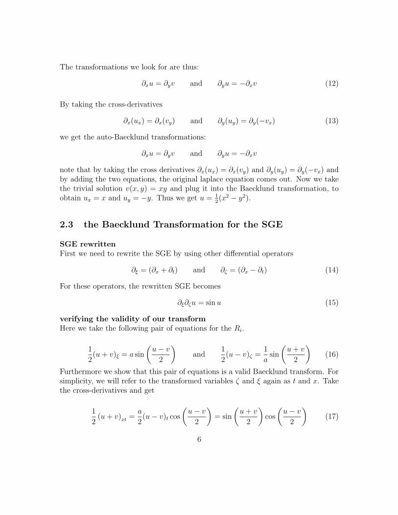
wavefunction”,Hi the total Hamilton operator for Si and T is the tunnel-coupling

i~∂tΦ1 = H1Φ1 + TΦ2 (40)

i~∂tΦ2 = H2Φ2 + TΦ1 (41)

If we now apply a voltage, and choose the origin symmetric, and also take Φ1 asan almost eigensolution with the energy eigenvalue qU , our equations can be rewrit-ten.

i~∂tΦ1 =qU

2Φ1 + TΦ2 (42)

i~∂tΦ2 =qU

2Φ2 + TΦ1 (43)

With |Φ|2 = ns/2 = nc as the density of cooper pairs, we rewrite our many particlewavefunction

Φ1 =√

nc1eiφ1 and Φ2 =

√nc2e

iφ2

then plugging in Φi in the equation (42) gives with separation of real and imaginaryparts

~/2∂tnc1 sin φ1 − (~∂tφ1 + qU/2) nc1 cos φ1 = T√

nc1nc2 cos φ2

~/2∂tnc1 cos φ1 − (~∂tφ1 + qU/2) nc1 sin φ1 = T√

nc1nc2 sin φ2

of course, there are analogous equations for the other equation (43)

Now we can multiply both equations with cos φ1 sin φ1 and the other way around andthen subtract from each equation the other equation to obtain a new set, togetherwith the same derivation for (43).

jT α ∂tnc1 =2

~T√

nc1nc2 sin(φ2 − φ1) (44)

jT α ∂tnc2 =−2

~T√

nc1nc2 sin(φ2 − φ1) (45)

∂tφ1 =1

~T

√nc2

nc1

cos(φ2 − φ1)−qU

2~(46)

∂tφ2 =1

~T

√nc1

nc2

cos(φ2 − φ1) +qU

2~(47)

14

What we get out is a proportionality for the tunneling current. This set can now besimplified for identical supraconductors (nc1 = nc2 = nc) to give the amazing resultthat there is an alternating current through the josephson junction, even though weapplied a constant voltage between the two superconductors. For the following wewill use the phase difference θ

∂tnc1 = (2T/~)nc sin(φ2 − φ1︸ ︷︷ ︸:=θ

) = −∂tnc2 = jT (48)

~(∂tφ2 − ∂tφ1) = −qU (49)

3.2.3 Elongated Josephson Junction

First note the homogeneous Maxwells equations and that E = ∂U∂x

= qUd

in onedimension

∇× E = −∂tB (50)

∇×B = µ0j + µ0ε∂tE (51)

without further explanation, note that there following ODE is valid for an ideal”resistively and capacitively shunted junction” for the external current

jB = jt +U

RS+

C

S

dU

dt(52)

where C is the capacity of the junction, R the resistivity, U the voltage, and S anarea. in this limit, for the josephson junction this equation becomes

d2

dt2θ +

1

RC

dθ

dt+ ω2

0 sin θ =2eS

C~jB (53)

which behaves like the equation for a disturbed excited pendulum

if we now insert (49 ) into the first of Maxwells equations, we get

−∂xEz = −∂x(U(x, t)/d) = −∂tBy (54)

⇔ ∂x(~

2ed∂tθ) = ∂tBy (55)

15

by integrating over time, we see

By =~

2ed∂xθ + B0y (56)

We can now insert this expression for the magnetic field in y-direction into the otherMaxwell equation.

uz∇×B = µ0j + µ0ε∂tE =~

2ed∂2

xθ + µ0jB (57)

inserting this last term into the junction equation instead of only µ0jB gives

θtt − c20θxx +

1

RCθt︸ ︷︷ ︸

A

+ω20 sin θ =

2eS

C~jB︸ ︷︷ ︸

B

which in some limit behaves like a SGE, provided the two terms A and B are small,which can experimentally be provided by designing the junction in the right way.One can through another calculation conclude that the solitons of the SGE providefluxons, that is a quantized magnetic flux.

4 Numerical Simulation

4.1 Another Notion For The SGE

The numerical examples were calculated using a Matlab program with a split stepFourier algorithm. Here we explain how it was programmed. Because this is a secondorder in time differential equation, we need first to get rid of one time differential.More precisely, note how we split the Sine Gordon equation: First, define

v =d

dtu (58)

Second, rewrite the sine Gordon equation as

−(

uv

)t

+

(0 1∂2

∂x2 0

)︸ ︷︷ ︸

:=L

(uv

)+

(0

sin(u)

)︸ ︷︷ ︸

:=S

= 0 , (59)

16

where the small t signifies taking the derivative with respect to time. For the simu-lations, we will start with given initial conditions and look at the time evolution ofthe problem. The split-step time evolution we then use is the following:

(uv

)(t + dt) = exp

(L

dt

2

)exp (Sdt) exp

(L

dt

2

)(uv

)(t) +O(dt3) (60)

where eSdt is a formal notation for the solution operator of the part(uv

)t

= S(u, v) (61)

The linear step exp(Ldt

2

)then can be solved using a fourier transform, as(

0 1∂2

∂x2 0

)=

(0 1−k2 0

)(62)

4.2 Pseudo-Code

The program thus works conceptually in the following way:

1. get initial conditions, that is a U0 :=(

u0

v0

)- vector.

⇒ Start the main loop

2. do a Fourier transform of U0

3. get U1 = LU0

4. inverse fourier transform of U1

5. perform nonlinear step using(

u2

v2

)=(

u1

dt sin(u1)

)

6. do a Fourier transform of U2

7. get U3 = LU2

17

8. inverse fourier transform of U3

⇒ get U(t + dt)

9. return to step 2

In principle, step 2 can be performed before starting the loop and then step 8 canbe omitted for efficiency reasons.

4.3 Programmed Examples

For the coded examples which you can find in the appendix, note that you needto change both the windows and the Length parameter of the simulation suitableto your problem, as you switch from one example to another. The code will storeyour data in a .avi-movieclip. The pictures have been made with the same code,but instead of getframe, use a matrix to which you store the according elementmeshmatrix(f,:)=uu(:); , and after the loop do mesh(meshmatrix)

As you can see in the appendix, there are many programmed examples, includinga test with an analytic and a numeric solution, to see deviations from the analyticsolution. An idea to improve the code would be to use twice as large vectors thatinclude both position and speed, and for the equation take a sparse matrix.

5 Appendix: Original Matlab Code

%%%%%%%%%%%%%%%%%%%%%%%%%%%%%%%%%%%%%%%%%%%%%%%%%%%%%%%%%%%%%%%%%%%%%%%%%%%%%%%%%%%%%%%%%%%%%%%%%%%%%%%%%%%%%%%%%%%%%%%%%%%%%%%%%%%%%%%%%%%Starting area%%%%%%%%%%%%%%%%%%%%%%%%%%%%%%%%%%%%%%%%%%%%%%%%%%%%%%%%%%%%%%%%%%%%%%%%%%%%%%%%%%%%%%%%%%%%%%%%%%%%%%%%%%%%%%%%%%%%%%%%%%%%%%%%%%%%%%%%%%

%%%%%%%%%%%%%%%%%%%%%%%%%%%%%%%%%%%%%%axis parameters for the plot%%%%%%%%%%%%%%%%%%%%%%%%%%%%%%%%%%%%%xmin = 0 ;

18

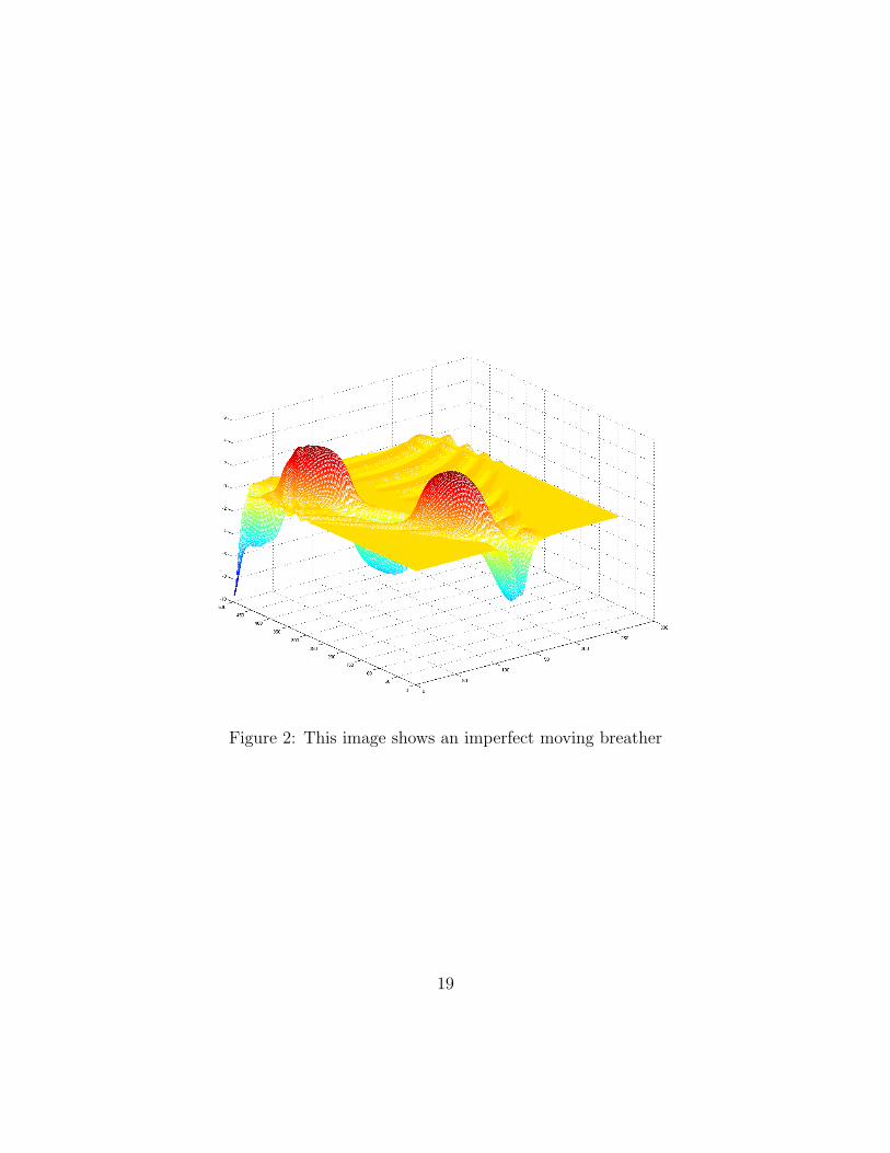
Figure 2: This image shows an imperfect moving breather

19

xmax = 2000 ;ymin = -7 ;ymax = 7 ;

%%%%%%%%%%%%%%%%%%%%%%%%%%%%%%%%%%%%%various starting parameters%%%%%%%%%%%%%%%%%%%%%%%%%%%%%%%%%%%%

t=0.01; %starting time for the propagating exact solutionlambda=0.992; %velocityconst=1; %other constant of integration for the solution

f=1; %frameparameter for the movieversetz=0; %distance between analytic and numeric solution

xo=1 %spatial breather parameterto=1 %time parameter for the breather

%%%%%%%%%%%%%%%%Of Space%%%%%%%%%%%%%%%

Nx = 257; %amount of discrete points in the x-space;L = 2000; %total length of the intervaldx = L/(Nx-1); %distance between two neighboring pointsx = linspace(0,L,Nx); %position space

%note: due to better efficiency of fft algorithm, Nx should be chosen as%2^n+1 , where the one additional point is needed for the doubling for the%interval

%%%%%%%%%%%%%%%%%%%And Time%%%%%%%%%%%%%%%%%%

Tfin = 1;dt = 0.01;Nt = floor(Tfin/dt);

20

%%%%%%%%%%%%%%%%%%%%%%%%%%%%%%%%%%%%%%%%%%%%%%%other parameters%%%%%%%%%%%%%%%%%%%%%%%%%%%%%%%%%%%%%%%%%%%%%%qu=(1-lambda^2)^0.5;

phii=const*exp((x-lambda*t)/qu);

%%%%%%%%%%%%%%%%%%%%%%%%%%%%%%%%%%%%%%%%% defining various vectors and matrices%%%%%%%%%%%%%%%%%%%%%%%%%%%%%%%%%%%%%%%%

F = zeros(2,Nx);FF = zeros(2,Nx);

uu = zeros(1,Nx);uv = zeros(1,Nx);

xx = zeros(1,Nx);yy = zeros(1,Nx);

% the transforming vectors

uuu = zeros(1,2);uuv = zeros(1,2);uvv = zeros(1,2);

% the transforming matrices

%transmat = [1 1; i*k -i*k];%eigvalmat = [ i*k 0 ; 0 -i*k];%invmat = [1/2 1/(2*i*k); 1/2 -1/(2*i*k)];%endmat=invmat*eigvalmat*transmat

%%%%%%%%%%%%%%%%%%%%%%%%%%%%%%%%%%%%%%%%%%% initial vectors%%%%%%%%%%%%%%%%%%%%%%%%%%%%%%%%%%%%%%%%%%

21

F(1,:) = 4*atan(const*exp((x-L/2-lambda*t)/qu));F(2,:) = -4*lambda*const*exp((x-L/2-lambda*t)/qu)./(qu*(1+const^2*exp(2*(x-L/2-lambda*t)/qu)));

%%%%%%%%%%%%%%%%%%%%%%%%%%%%%%%%%%%%%%% self generation of a soliton%%%%%%%%%%%%%%%%%%%%%%%%%%%%%%%%%%%%%%

%F(1,:) = 4*(atan((x-L/2-lambda*t)/qu)+pi/2)/2;%F(2,:) = -abs(lambda*const*(1/qu)./(qu*(1+const^2*(x-L/2-lambda*t).^2/qu)));

%%%%%%%%%%%%%%%%%%%%%%%%%%%% Soliton interactions%%%%%%%%%%%%%%%%%%%%%%%%%%%

%a = linspace(0,L/2,Nx/2);%b = linspace(L/2,L,Nx/2);

%AA = 4*atan(const*exp((-a+L/4-lambda*t)/qu));%aaa = 4*lambda*const*exp((a-L/4-lambda*t)/qu)./(qu*(1+const^2*exp(2*(a-L/4-lambda*t)/qu)));

%BB = -4*atan(const*exp((b-L*3/4-lambda*t)/qu));%bbb = -4*lambda*const*exp((b-L*3/4-lambda*t)/qu)./(qu*(1+const^2*exp(2*(b-L*3/4-lambda*t)/qu)));

%F(1,:)=[AA 0 BB];%F(2,:)=[aaa 0 bbb];

%axis([xmin xmax ymin ymax])%plot(x,F’)%pause(0.5)

%%%%%%%%%%%%%%%%%%%%%%%%%%%%%%%%%%%%%%% more complicated interactions%%%%%%%%%%%%%%%%%%%%%%%%%%%%%%%%%%%%%%

%a = linspace(0, L/4, Nx/4);%b = linspace(L/4, L/2, Nx/4);%c = linspace(L/2, L*3/4, Nx/4);%d = linspace(L*3/4, L, Nx/4);

%AA = 4*atan(const*exp((a-L/8-lambda*t)/qu));%aaa = -4*lambda*const*exp((a-L/8-lambda*t)/qu)./(qu*(1+const^2*exp(2*(a-L/8-lambda*t)/qu)));

%BB = 4*atan(const*exp((-b+L*3/8-lambda*t)/qu));%bbb = 4*lambda*const*exp((b-L*3/8-lambda*t)/qu)./(qu*(1+const^2*exp(2*(b-L*3/8-lambda*t)/qu)));

22

%CC = -4*atan(const*exp((c-5*L/8-lambda*t)/qu));%ccc = 4*lambda*const*exp((c-5*L/8-lambda*t)/qu)./(qu*(1+const^2*exp(2*(c-5*L/8-lambda*t)/qu)));

%DD = -4*atan(const*exp((-d+L*7/8-lambda*t)/qu));%ddd = -4*lambda*const*exp((d-L*7/8-lambda*t)/qu)./(qu*(1+const^2*exp(2*(d-L*7/8-lambda*t)/qu)));

%fff=[AA BB CC 0 DD ];%ffff=[aaa bbb 0 ccc ddd];%F(1,:)=[AA BB 0 CC DD];%F(2,:)=[aaa bbb 0 ccc ddd];

%%%%%%%%%%%%%%%%%%%%%%%%%%%%%%%%%%%%%%%%%%%%%%%completely non-solitonic initial conditions%%%%%%%%%%%%%%%%%%%%%%%%%%%%%%%%%%%%%%%%%%%%%%

%a = linspace(0, L/4, Nx/4);%b = linspace(L/4, L*3/4, Nx/2);%c = linspace(L*3/4, L, Nx/4);

%F(1,:) = [a*0 0 4*sin(b) c*0];%F(2,:) = [a*0 0 4*cos(b) c*0];

%or other variant%a = linspace(0, L*9/40, Nx/4);%b = linspace(L*9/40, L*31/40, Nx/2);%c = linspace(L*31/40, L, Nx/4);

%F(1,:) = [a*0 0 6*exp(-(4*cos(b)).^2) c*0];%F(2,:) = [a*0 0 6*sin(b).*cos(b).*exp(-(4*cos(b)).^2) c*0];

%instead: how a point excitation at the middle of the interval behaves% like a chain of pendula

%F(1,int16(Nx/2))=4%F(2,int16(Nx/2))=0

%%%%%%%%%%%%%%%%%%%%%%%%%%%%%%%%%%%%%%%%%%%%%%

23

% breather%%%%%%%%%%%%%%%%%%%%%%%%%%%%%%%%%%%%%%%%%%%%%%

% note for the breather stuff: here the derivative can be taken numerically,% by the diff function. thus the derivative is one element shorter than a "typical" derivative,%thus the derivative gets shifted by 1/2, this might lead to rather big errors

%aa=2*4*atan(qu/lambda*sin(lambda*(t-to))./cosh(qu*(x-L/2-xo)))%bb=diff([0 aa])/dx%bb=-8*qu^2/lambda*sin(lambda*(t-1))./cosh(qu*(x-L/2-1)).^2.*sinh(qu*(x-L/2-1))./(1+qu^2/%lambda^2*sin(lambda*(t-1))^2./cosh(qu*(x-L/2-1)).^2)

%F(1,:)=aa%F(2,:)=bb

%%%%%%%%%%%%%%%%%%%%%%%%%%%%%%%%%%%%%%%%%%%%%%% a kink-antikink pair en detail%%%%%%%%%%%%%%%%%%%%%%%%%%%%%%%%%%%%%%%%%%%%%%

%aa=4*atan(lambda*cosh((x-L/2)/qu)/sinh(lambda*t/qu))%bb=4*lambda*sinh((x-L/2)/qu)/qu/sinh(lambda*t/qu)./(1+lambda^2*cosh((x-L/2)/qu).^2/%sinh(lambda*t/qu)^2)

%F(1,:)=aa%F(2,:)=bb

%%%%%%%%%%%%%%%%%%%%%%%%%%%%%%%%%%%%looking at our initial conditions%%%%%%%%%%%%%%%%%%%%%%%%%%%%%%%%%%%

axis([xmin xmax ymin ymax])plot(x,F’)pause(0.5)

%%%%%%%%%%%%%%%%%%%%%%%%%%%%%%%%%%%%%%%%%%%%%%%%%%%%%%%%%%%%%%%%%%%%%%%%%%%%%%%%%%%%%%%%%%%%%%%%%%%%%%%%%%%%%%%%%%%%%%%%%%%%%%%%%%%%%%%%%%%here comes the fun ...%%%%%%%%%%%%%%%%%%%%%%%%%%%%%%%%%%%%%%%%%%%%%%%%%%%%%%%%%%%%%%%%%%%%%%%%%%%%%%%%%%%%%%%%%%%%%%%%%%%%%%%%%%%%%%%%%%%%%%%%%%%%%%%%%%%%%%%%%%

24

% 0. getting vectors and their fourier transforms

for i=1:Nxuu(1,i)=F(1,i);uv(1,i)=F(2,i);

end

% Looking at the initial values and including in the movieplot(x, F’)M(1)=getframe;%M(2)=getframe;

xx = fft([uu uu(end-1:-1:2)],2*Nx-2);yy = fft([uv uv(end-1:-1:2)],2*Nx-2);qq = fftshift(xx);qz = fftshift(yy);

% 1. Begin main loop

for r=2:Nt

% 2. Piecewise construction of the first t/2 part

for p=1:2*Nx-2uuu(1,1) = qq(1,p);uuu(1,2) = qz(1,p);

k = (pi/L)*(-Nx+p);Mmat =[0 1; -k^2 0];

uuu = expm(Mmat*dt/2)*transpose(uuu);

qq(1,p) = uuu(1,1);qz(1,p) = uuu(2,1);

end

25

% 3. Nonlinear part of the SGE :

% backtransforming into real spacexx = ifftshift(qq);yy = ifftshift(qz);xx = ifft(xx, 2*Nx-2);yy = ifft(yy, 2*Nx-2);uu = xx(1:Nx);uv = yy(1:Nx);for q=1:Nx

%su(1,q) = uu(1,q)%sv(1,q) = dt*sin(uv(1,q))+uu(1,q)%uu(1,q) = uu(1,q)uv(1,q) = -dt*sin(uu(1,q)) + uv(1,q) ;

%For the PlotFF(1,q)=abs(uu(1,q));FF(2,q)=abs(uv(1,q));%%%%%%%%%%%%%%%

endxx = fft([uu uu(end-1:-1:2)],2*Nx-2);yy = fft([uv uv(end-1:-1:2)],2*Nx-2);qq = fftshift(xx);qz = fftshift(yy);

%5. second t/2 part

for p=1:2*Nx-2uuu(1,1) = qq(1,p);uuu(1,2) = qz(1,p);

k = (pi/L)*(-Nx+p);Mmat =[0 1; -k^2 0];

uuu = expm(Mmat*dt/2)*transpose(uuu);

qq(1,p) = uuu(1,1);qz(1,p) = uuu(2,1);

end

%print out curr. timer

26

if(mod(r,5)==0)

% backtransforming into real spacexx = ifftshift(qq);yy = ifftshift(qz);xx = ifft(xx, 2*Nx-2);yy = ifft(yy, 2*Nx-2);uu = xx(1:Nx);uv = yy(1:Nx);

figure(1)axis([xmin xmax ymin ymax])plot(x,uu)hold onaxis([xmin xmax ymin ymax])plot(x,uv, ’r’)

%plot exact sol.% t=(r+2)*dt;% F(1,:) = 4*atan(const*exp((x-L/2-lambda*t-lambda*versetz)/qu));% F(2,:) = -4*lambda*const*exp((x-L/2-lambda*t-lambda*versetz)/qu)./(qu*(1+const^2*exp(2*(x-L/2-lambda*t-lambda*versetz)/qu)));% axis([xmin xmax ymin ymax])% plot(x,F(1,:), ’--’)% axis([xmin xmax ymin ymax])% plot(x,F(2,:), ’r--’)% axis([xmin xmax ymin ymax])hold offtitle(sprintf(’t=%g’,t))pause(0.01)M(f)=getframe;f=f+1;

end

end

%showing & saving the moviemovie(M ,1)movie2avi(M, ’kinkantikinkpairgeneration.avi’)

27

References

[1] P.G. Drazin, R.S. Johnson, Solitons: an introduction, Cambridge UniversityPress, ISBN 0-521-33655-4, 1990

[2] M. Peirard, T. Dauxois, Physique des solitons , EDP Sciences-CNRS Editions,ISBN 2-271-06267-5, 2004

[3] H. Ibach, H. Lueth, Festkoerperphysik , Springer-Verlag, ISBN 2-271-06267-5,2002

28