Notes on the Reidemeister Torsion - University of Notre Damelnicolae/Torsion.pdf · Notes on the...
259
Notes on the Reidemeister Torsion Liviu I. Nicolaescu University of Notre Dame Notre Dame, IN 46556 http://www.nd.edu/ ˜ lnicolae/ January 2002
Transcript of Notes on the Reidemeister Torsion - University of Notre Damelnicolae/Torsion.pdf · Notes on the...

Notes on the Reidemeister Torsion
Liviu I. NicolaescuUniversity of Notre Dame
Notre Dame, IN 46556http://www.nd.edu/˜ lnicolae/
January 2002

To the memory of my father, Ion I. Nicolaescu,
who shared with me his passion for books.

Introduction
The torsion of a cellular (simplicial) complex was introduced in the 30s by W. Franz[29] and K. Reidemeister [90] in their study of lens spaces. The lens spaces L(p, q)(p fixed) have the same fundamental groups and thus the same homology groups.However, they are not all homeomorphic. They are not even homotopically equivalent.This can be observed by detecting some below the radar interactions between thefundamental group and the simplicial structure. The torsion captures some of theseinteractions. In particular, it is able to distinguish lens spaces which are homotopicallyequivalent but not homeomorphic, and moreover completely classify these spaces upto a homeomorphism. This suggests that this invariant is reaching deep inside thetopological structure.
What is then this torsion? What does is compute? These are the kind of ques-tions we try to address in these notes, through many examples and various equivalentdescriptions of this invariant.
From an algebraic point of view, the torsion is a generalization of the notion ofdeterminant. The most natural and general context to define the torsion would involvethe Whitehead group and algebraic K-theory as in the very elegant and influentialMilnor survey [72], but we did not adopt this more general point of view. Instead welook at what Milnor dubbed R-torsion.
This invariant can be viewed as a higher Euler characteristic type invariant. Muchlike the Euler characteristic, the torsion satisfies an inclusion-exclusion (a.k.a. Mayer–Vietoris) principle which can be roughly stated as
Tors(A ∪ B) = Tors(A)+ Tors(B)− Tors(A ∩ B)which suggests that the torsion could be interpreted as counting something.
The classical Poincaré–Hopf theorem states that the Euler–Poincaré characteristicof a smooth manifold counts the zeros of a generic vector field. If the Euler-Poincarécharacteristic is zero then most vector fields have no zeroes but may have periodicorbits. The torsion counts these closed orbit, at least for some families of vector fields.As D. Fried put it in [34], “the Euler characteristic counts points while the torsioncounts circles”.
One of the oldest results in algebraic topology equates the Euler-Poincaré char-acteristic of simplicial complex, defined as the alternating sums of the numbers ofsimplices, with a manifestly combinatorial invariant, the alternating sum of the Bettinumbers. Similarly, the R-torsion can be given a description in terms of chain com-plexes or, a plainly invariant description, in homological terms. Just like the Eulercharacteristic, the R-torsion of a smooth manifold can be given a Hodge theoreticdescription, albeit much more complicated.
More recently, this invariant turned up in 3-dimensional Seiberg–Witten theory, inthe work of Meng–Taubes ([68]). This result gave us the original impetus to understand

Introduction vii
the meaning of torsion.This is a semi-informal, computationally oriented little book which grew out of
our efforts to understand the intricacies of the Meng–Taubes–Turaev results, [68, 115].For this reason a lot of emphasis is placed on the Reidemeister torsion of 3-manifolds.These notes tried to address the author’s own struggle with the overwhelming amountof data involved and the conspicuously scanty supply of computational examples inthe traditional literature on the subject. We considered that at an initial stage a goodintuitive argument or example explaining why a certain result could be true is morehelpful than a complete technical proof. The classical Milnor survey [72] and therecent introductory book [117] by V. Turaev are excellent sources to fill in many ofour deliberate foundational omissions.
When thinking of topological issues it is very important not to get distracted by theugly looking but elementary formalism behind the torsion. For this reason we devotedthe entire first chapter to the algebraic foundations of the concept of torsion. We giveseveral equivalent definitions of the torsion of an acyclic complex and in particular,we spend a good amount of time constructing a setup which coherently deals with thetorturous sign problem. We achieved this using a variation of some of the ideas inDeligne’s survey [18].
The general algebraic constructions are presented in the first half of this chapter,while in the second half we discuss Turaev’s construction of several arithmeticallydefined subrings of the field of fractions of the rational group algebra of an Abeliangroup. These subrings provide the optimal algebraic framework to discuss the torsionof a manifold. We conclude this chapter by presenting a dual picture of this Turaevsubrings via Fourier transform. These results seem to be new and simplify substantiallymany gluing formulæ for the torsion, to the point that they become quasi-tautological.
The Reidemeister torsion of an arbitrary simplicial (or CW) complex is defined inthe second chapter. This is simply the torsion of a simplicial complex with Abelianlocal coefficients, or equivalently the torsion of the simplicial complex of the maximalAbelian cover. We present the basic properties of this invariant: the Mayer–Vietorisprinciple, duality, arithmetic properties and an Euler–Poincaré type result. We com-pute the torsion of many mostly low dimensional manifolds and in particular we explainhow to compute the torsion of any 3-manifold with b1 > 0 using the Mayer–Vietorisprinciple, the Fourier transform, and the knowledge of the Alexander polynomials oflinks in S3. Since the literature on Dehn surgery can be quite inconsistent on thevarious sign conventions, we have devoted quite a substantial appendix to this subjectwhere we kept an watchful eye on these often troublesome sings.
The approach based on Alexander polynomials has one major drawback, namely itrequires a huge volume of computations. We spend the whole section §2.6 explaininghow to simplify these computation for a special yet very large class of 3-manifolds,namely the graph manifolds. The links of isolated singularities of complex surfaces areincluded in this class and the recent work [75, 76] proves that the Reidemeister torsioncaptures rather subtle geometrical information about such manifolds. We concludethis chapter with some of the traditional applications of the torsion in topology.
viii Introduction
Chapter 3 focuses on Turaev’s ingenious idea of Euler structure and how it canbe used to refine the concept of torsion by removing the ambiguities in choosing thebases needed for computing the torsion. Turaev later observed that for a 3-manifolda choice of an Euler structure is equivalent to a choice of spinc-structure. After wereview a few fundamental properties of this refined torsion for 3-manifolds we thengo on to present a result of Turaev which in essence says that the refined torsion of a3-manifold with positive b1 is uniquely determined by the Alexander polynomials oflinks in S3 and the Mayer–Vietoris principle.
This uniqueness result does not include rational homology spheres, and thus offersno indication on how to approach this class of manifolds. We spend the last part ofthis chapter analyzing this class of 3-manifolds.
In §3.8 we describe a very powerful method for computing the torsion of such3-manifolds, based on the complex Fourier transform results in Chapter 1, and anextremely versatile holomorphic regularization technique. These lead to explicit for-mulæ for the Fourier transform of the torsion of a rational homology sphere in terms ofsurgery data. These formulæ still have the two expected ambiguities: a sign ambiguityand a spinc ambiguity. In §3.9 we describe a very simple algorithm for removing thespinc ambiguity. This requires a quite long topological detour in the world of quadraticfunctions on finite Abelian groups, and surgery descriptions of spin and spinc struc-tures, but the payoff is worth the trouble. The sign ambiguity is finally removed in§3.10 in the case of plumbed rational homology spheres, relying on an idea in [75],based on the Fourier transform, and a relationship between the torsion and the linkingform discovered by Turaev.
Chapter 4 discusses more analytic descriptions of the Reidemeister torsion: interms of gauge theory, in terms of Morse theory, and in terms of Hodge theory. Wediscuss Meng–Taubes theorem and the improvements due to Turaev. We also out-line our recent proof [83] of the extension of the Meng–Taubes–Turaev theorem torational homology spheres. As an immediate consequence of this result, we give anew description of the Brumfiel–Morgan [7] correspondence for rational homology3-spheres which associates to each spinc structure a refinement of the linking form.
On the Morse theoretic side we describe Hutchinson–Pajitnov results which givea Morse theoretic interpretation of the Reidemeister torsion. We barely scratch theHodge theoretic approach to torsion. We only provide some motivation for the ζ -function description of the analytic torsion and the Cheeger–Müller theorem whichidentifies this spectral quantity with the Reidemeister torsion.
∗ ∗ ∗
Acknowledgements1 I spent almost two years thinking about these issues and I washelped along the way by many people. I am greatly indebted to Frank Connolly whointroduced me to this subject. His patience and expertise in answering my often half
1This work was partially supported by NSF grant DMS-0071820.

Introduction ix
baked questions have constantly kept me on the right track. I also want to thank mycolleagues Bill Dwyer, Stephan Stolz, Larry Taylor and Bruce Williams for manyilluminating discussions which made this scientific journey so much more enjoyable.
This survey started up as a set of study notes to myself with no large audience inmind. They may have not seen the “light of day” were it not for Andrew Ranicki’sinterest and support. I want to thank him for the insightful comments concerning thesenotes which have substantially helped me to improve the quality of the presentation.
I want to thank Vladimir Turaev whose work had a tremendous influence on theway I think about this subject. I appreciate very much his interest in these notes, andhis helpful suggestions.
The sections §3.8, §3.9 and §3.10 are a byproduct of the joint work with AndrásNémethi, [75, 76]. I want use this opportunity to thank him for our very exciting andstimulating collaboration.
I performed the final revision of the manuscript during my sabbatical leave at theOhio State University. I want to express my gratitude to Dan Burghelea for his verywarm and generous hospitality, and his contagious enthusiasm about mathematics,and culture in general.
At last but not the least I want to thank my family for always being there for me.
Notre Dame, Indiana 2002 Liviu I. Nicolaescu

Notations and conventions
• For simplicity, unless otherwise stated, we will denote byH∗(X) the homology withintegral coefficients of the topological space X.
• For K = R,C, we denote by KnX the trivial rank n, K-vector bundle over the spaceX.
• i := √−1.
• u(n) = the Lie algebra of U(n), su(n)= the Lie algebra of SU(n) etc.
• Z+ = Z≥0 := {n ∈ Z; n ≥ 0}.• For all integers m < n we set m, n := Z ∩ [m, n].• For any Abelian group G we will denote by Tors(G) its torsion subgroup. We willuse the notation Zn := Z/nZ.
• If R is a commutative ring with 1, then R× denotes the group of invertible elementsof R.
•Also, we will strictly adhere to the following orientation conventions.
• If M is an oriented manifold with boundary then the induced orientation of ∂M isdetermined by the outer-normal-first convention
or (M) = outer normal ∧ or (∂M).
• If F ↪→ E � B is a smooth fiber bundle, where F and B are oriented, then theinduced orientation of E is determined by the fiber-first convention
or (E) = or (F ) ∧ or (B).

Contents
Introduction vi
Notations and conventions xi
1 Algebraic preliminaries 1§1.1 The torsion of acyclic complexes of vector spaces . . . . . 1§1.2 The determinant line of a chain complex . . . . . . . . . . 7§1.3 Basic properties of the torsion . . . . . . . . . . . . . . . 16§1.4 Some generalizations . . . . . . . . . . . . . . . . . . . . 20§1.5 Abelian group algebras . . . . . . . . . . . . . . . . . . . 21§1.6 Abelian harmonic analysis . . . . . . . . . . . . . . . . . 30
2 The Reidemeister torsion 44§2.1 The Reidemeister torsion of a CW-complex . . . . . . . . 44§2.2 Fitting ideals . . . . . . . . . . . . . . . . . . . . . . . . 59§2.3 The Alexander function and the Reidemeister torsion . . . 63§2.4 The Reidemeister torsion of 3-manifolds . . . . . . . . . . 67§2.5 Computing the torsion of 3-manifolds using surgery pre-
sentations . . . . . . . . . . . . . . . . . . . . . . . . . . 70§2.6 Plumbings . . . . . . . . . . . . . . . . . . . . . . . . . . 83§2.7 Applications . . . . . . . . . . . . . . . . . . . . . . . . . 102
3 Turaev’s refined torsion 106§3.1 Combinatorial Euler structures . . . . . . . . . . . . . . . 106§3.2 Smooth Euler structures . . . . . . . . . . . . . . . . . . . 108§3.3 U(2) and Spinc(3) . . . . . . . . . . . . . . . . . . . . . . 115§3.4 Euler structures on 3-manifolds . . . . . . . . . . . . . . . 120§3.5 The Reidemeister–Turaev torsion of Euler structures . . . 126§3.6 Arithmetic properties of the Reidemeister–Turaev torsion
of 3-manifolds . . . . . . . . . . . . . . . . . . . . . . . . 127§3.7 Axiomatic description of the Reidemeister–Turaev torsion
of 3-manifolds . . . . . . . . . . . . . . . . . . . . . . . . 131§3.8 The torsion of rational homology 3-spheres. Part 1. . . . . 135§3.9 Quadratic functions, spinc structures and charges . . . . . 148§3.10 The torsion of rational homology 3-spheres. Part 2. . . . . 164

xiv Introduction
4 Alternative interpretations of the Reidemeister torsion 174§4.1 A gauge theoretic interpretation: Seiberg–Witten invariants 174§4.2 A Morse theoretic interpretation . . . . . . . . . . . . . . 187§4.3 A spectral interpretation: the Ray–Singer analytic torsion . 193
A Algebra 197§A.1 Formal Hodge theory . . . . . . . . . . . . . . . . . . . . 197§A.2 Determinants and zeta functions . . . . . . . . . . . . . . 202§A.3 Extensions of Abelian groups . . . . . . . . . . . . . . . . 205
B Topology 210§B.1 How to compute the Alexander polynomial of a knot . . . 210§B.2 Dehn surgery and linking forms . . . . . . . . . . . . . . 216
Bibliography 239
Index 244

Chapter 1
Algebraic preliminaries
§1.1 The torsion of acyclic complexes of vector spaces
The notion of torsion is a multifaceted generalization of the concept of determinant ofan isomorphism of vector spaces. We begin with a baby example to give the reader ataste of the ingredients which enter into the fabric of torsion, and of the type of issuesit addresses.
Example 1.1. Suppose that U0 and U1 are finite dimensional real vector spaces andS, T : U1 → U0 are two linear isomorphisms. If we take into account only the vectorspace structures then we could consider S and T to be equivalent, i.e. there existAi ∈ Aut(Ui), i = 0, 1, such that
T = A0SA−11 . (1.1)
Suppose now that �i ⊂ Ui , i = 0, 1 are lattices and S, T are compatible withthem, i.e. S(�1) ⊂ �0, T (�1) ⊂ �0. We could then ask whether there existAi ∈ Aut(�i) ⊂ Aut(Ui), i = 0, 1, such that (1.1) holds. We can easily construct aninvariant to show that S and T need not always be equivalent in this more restrictedsense. Consider for example the finite Abelian groups
I (S) = �0/S(�1), I (T ) = �0/T (�1).
If S is equivalent to T then |I (S)| = |I (T )| and we see that the quantity S → |I (S)| isan invariant of this restricted equivalence relation. It is very easy to compute it. PickZ-bases of �i , i = 0, 1. We can then identify S and T with integral matrices and, upto a sign, |I (S)| and |I (T )| are the determinants of these matrices.
The torsion tackles a slightly more general question than this. This generalityentails several aspects, all motivated by topological issues. First, instead of lattices inreal vector spaces we will work with free modules over a commutative ringR. Insteadof the field of real numbers we will work with a fieldK related toR via a nontrivial ringmorphism χ : R→ K. If F is a freeR module then F ⊗χ K is aK-vector space. Therole of the groups Aut(�i) we will played by certain subgroups of AutR(F ), whichact in an obvious way on F ⊗χ K. Finally, instead of morphisms of R-modules wewill consider chain complexes of R-modules. �
We will begin our presentation by discussing the notion of torsion (or determinant)of a chain complex of finite dimensional vector spaces. In the sequel, K will denotea field of characteristic zero. A basis of a K-vector space will be a totally orderedgenerating set of linearly independent vectors.
2 1 Algebraic preliminaries
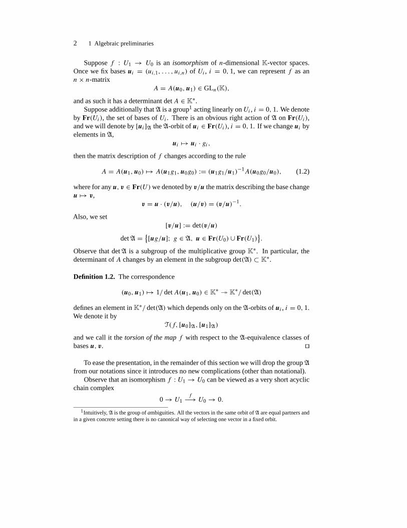
Suppose f : U1 → U0 is an isomorphism of n-dimensional K-vector spaces.Once we fix bases ui = (ui,1, . . . , ui,n) of Ui , i = 0, 1, we can represent f as ann× n-matrix
A = A(u0,u1) ∈ GLn(K),
and as such it has a determinant detA ∈ K∗.Suppose additionally that A is a group1 acting linearly on Ui , i = 0, 1. We denote
by Fr (Ui), the set of bases of Ui . There is an obvious right action of A on Fr (Ui),and we will denote by [ui]A the A-orbit of ui ∈ Fr (Ui), i = 0, 1. If we change ui byelements in A,
ui → ui · gi,then the matrix description of f changes according to the rule
A = A(u1,u0) → A(u1g1,u0g0) := (u1g1/u1)−1A(u0g0/u0), (1.2)
where for any u, v ∈ Fr (U)we denoted by v/u the matrix describing the base changeu → v,
v = u · (v/u), (u/v) = (v/u)−1.
Also, we set[v/u] := det(v/u)
det A = {[ug/u]; g ∈ A, u ∈ Fr (U0) ∪ Fr (U1)}.
Observe that det A is a subgroup of the multiplicative group K∗. In particular, thedeterminant of A changes by an element in the subgroup det(A) ⊂ K∗.
Definition 1.2. The correspondence
(u0,u1) → 1/ detA(u1,u0) ∈ K∗ � K∗/ det(A)
defines an element in K∗/ det(A) which depends only on the A-orbits of ui , i = 0, 1.We denote it by
T(f, [u0]A, [u1]A)and we call it the torsion of the map f with respect to the A-equivalence classes ofbases u, v. �
To ease the presentation, in the remainder of this section we will drop the group Afrom our notations since it introduces no new complications (other than notational).
Observe that an isomorphism f : U1 → U0 can be viewed as a very short acyclicchain complex
0 → U1f−→ U0 → 0.
1Intuitively, A is the group of ambiguities. All the vectors in the same orbit of A are equal partners andin a given concrete setting there is no canonical way of selecting one vector in a fixed orbit.

§1.1 The torsion of acyclic complexes of vector spaces 3
The notion of torsion described above extends to acyclic chain complexes of arbitrarysizes. Suppose that
C := 0 → Cn∂n→ Cn−1
∂n−1→ · · · ∂1→ C0 → 0
is an acyclic, complex of finite dimensional K-vector spaces. Fix bases ci of Ci .Because C is acyclic there exists an algebraic contraction, i.e. a degree one map
η : Ci → Ci+1
such that∂η + η∂ = 1C.
(See Appendix §A.1.) Set η = η∂η.
Exercise 1.1. (a) Prove that η is an algebraic contraction satisfying η2 = 0.
(b) Show that if η2 = 0 then η = η. �
Consider the operator∂ + η : C → C.
It satisfies(∂ + η)2 = ∂η + η∂ = 1,
so that it is an isomorphism. Moreover, with respect to the direct sum decomposition
C = Ceven ⊕ Codd
it has the block form
∂ + η =[
0 T01T10 0
], T01 : Codd → Ceven, T10 : Ceven → Codd.
We deduce that T10 is an isomorphism of vector spaces and T −110 = T01. We can define
T(C, c) := T
(∂ + η, [ceven
],[codd
]) = det(∂ + η : Codd → Ceven
)−1
= det(∂ + η : Ceven → Codd
).
We need to be more specific about codd and ceven. If we denote by 2m+ 1 (resp. 2ν)the largest odd (resp. even) number not greater than the length of C then
codd = c2m+1 ∪ · · · ∪ c3 ∪ c1, ceven = c2ν ∪ · · · ∪ c2 ∪ c0. (1.3)
Proposition 1.3([19]). det(∂+η : Ceven → Codd
)is independent of the choice of η.

4 1 Algebraic preliminaries
Proof. Suppose η0, η1 are two algebraic contractions. Set η := η1−η0, ηt = η0+ t η.Observe that η∂ = −∂η and ηt is an algebraic contraction of C. Moreover
ηt+s = (ηt + sη)∂(ηt + sη) = ηt + s(η∂ηt + ηt∂η)+ s2η∂η.
We set Tt := ∂ + ηt and η′t = dds|s=0ηt+s = η∂ηt + ηt∂η. Derivating2 the identities
η2t = 0, ∂ηt + ηt ∂ = 1,
we deduce thatηt η
′t = −η′t ηt , ∂η′t = −η′t ∂.
This shows that Tt η′t = −η′t Tt . Using the identity T 2t = 1 we obtain
Tt+s = ∂ + ηt+s = Tt + sηt = Tt(1+ sTt η′t
).
To prove that det(Tt : Ceven → Codd) is independent of t it suffices to show that
tr(Tt η′t : Ceven → Ceven) = 0.
Observe thatTt η
′t = (ηt η∂ηt + ηt ηt ∂η)+ ∂η =: A+ B.
Since A(Ck) ⊂ Ck+2, we deduce tr(A) = 0. Next, consider the filtration Ceven ⊃ker ∂ ⊃ Im ∂ ⊃ 0. Observe that BCeven ⊂ Im ∂ and B acts trivially on ker ∂ . Thisshows that trB = 0 and completes the proof of the proposition. �
Definition 1.4. The quantity T(C, c) is called the torsion of the acyclic complex Cwith respect to the bases c. �
Observe that if c′ is another basis of C then using (1.2) we deduce
T(C, c′) = T(C, c)
n∏i=0
[c′i/ci](−1)i . (1.4)
Convention. When the complex C is not acyclic we define its torsion to be 0.
We can alternatively define the torsion as follows. Choose finite, totally orderedcollections bi ⊂ Ci of such that the restriction of ∂ to bi is one-to-one for all i, b0 = ∅,and
∂bi+1 ∪ bi is a basis of Ci . (†)
(This condition uses the acyclicity of C.) Now set c := ⊕ici , and define the torsionof C with respect to the bases ci by
T(C, [c]A) :=n∏i=0
[(∂bi+1)bi/ci](−1)i+1 ∈ K∗/ det(A). (1.5)
2The derivatives are understood in the formal sense, as linearizations.

§1.1 The torsion of acyclic complexes of vector spaces 5
The relationship between these two definitions is very simple. Let us first introducea notation. If X is a basis of a vector space U , and u is a vector in U , then thedecomposition of u along this basis will be denoted by
u :=∑x∈X〈u|x〉x.
Given collections bi as above we define a contraction η : C → C,
Ci � u =∑b∈bi+1
〈u|∂b〉∂b +∑b′∈bi
〈u|b′〉b′ →∑b∈bi+1
〈u|∂b〉b ∈ Ci+1.
We define c′i = ∂bi+1 ∪ bi . Then
T(C, c′) = det(∂ + η : (Ceven, c
′even)→ (Codd, c
′odd)) = 1.
The equality (1.5) now follows by invoking the transition formula (1.4).We present below another simple and effective way of performing concrete com-
putations.
Proposition 1.5([38, 110]).3 Suppose C is an acyclic complex of finite dimensionalK-vector spaces. Denote by � the length of C, fix a basis c of C and denote byDi thematrix of the linear operator
∂ : Ci+1 → Ci
with respect to the chosen bases. Set
ni := dimK Ci, si := dimK ker(∂ : Ci → Ci−1).
Assume there exists a τ -chain, i.e. a collection{(Si, Di); Si ⊂ 1, ni, si = |Si |, i = 0, 1, . . . , �− 1, Di : Kni+1−si+1 → Ksi
}such that the matrix Di obtained from Di by deleting the columns belonging to Si+1and the rows belonging to 1, ni \ Si is quadratic and nonsingular (see Figure 1.1).Then
T(C, c) =�−1∏i=0
det(Di)(−1)i+1+νi
,
whereνi :=
∣∣{(x, y) ∈ Z× Z; 1 ≤ x < y, x ∈ 1, ni \ Si, y ∈ Si}∣∣.
3This result has a long history, going back to A. Cayley [12].

6 1 Algebraic preliminaries
Si+1
1, ni+1 \ Si+1Di+1
ni+1 − si+1 = si
1, ni \ Si
Si
Figure 1.1. Visualizing a τ -chain.
Proof. Letci := {ci,1, . . . , ci,ni }.
Definebi := {ci,j ; j �∈ Si}
where the above vectors are arranged in the increasing order given by j . The bases bisatisfy the condition (†) and moreover,
[∂bi+1bi/ci] = (−1)νi det(Di). �
Example 1.6(Algebraic mapping torus, [33, 34]). A useful operation one can per-form on chain complexes is the algebraic mapping torus construction, [33]. Moreprecisely, suppose (C, ∂) is a chain complex of K-vector spaces, c is a basis of C and
f : C → C
is a chain morphism, i.e. a degree zero map commuting with ∂ . The algebraic mappingtorus of C with respect to f is the chain complex
(T (f ), ∂f ), T (f )k := Ck ⊕ Ck−1,
∂f :Ck⊕Ck−1
→Ck−1⊕Ck−2
,
uv
→ ∂ (1− f )
0 −∂
· uv
The bases c define bases T (c) in T (f ), unique up to ordering. Assume det(1− f ) ∈K∗. Then the map
η : T (f )k → T (f )k+1, η = 0 0
(1− f )−1 0
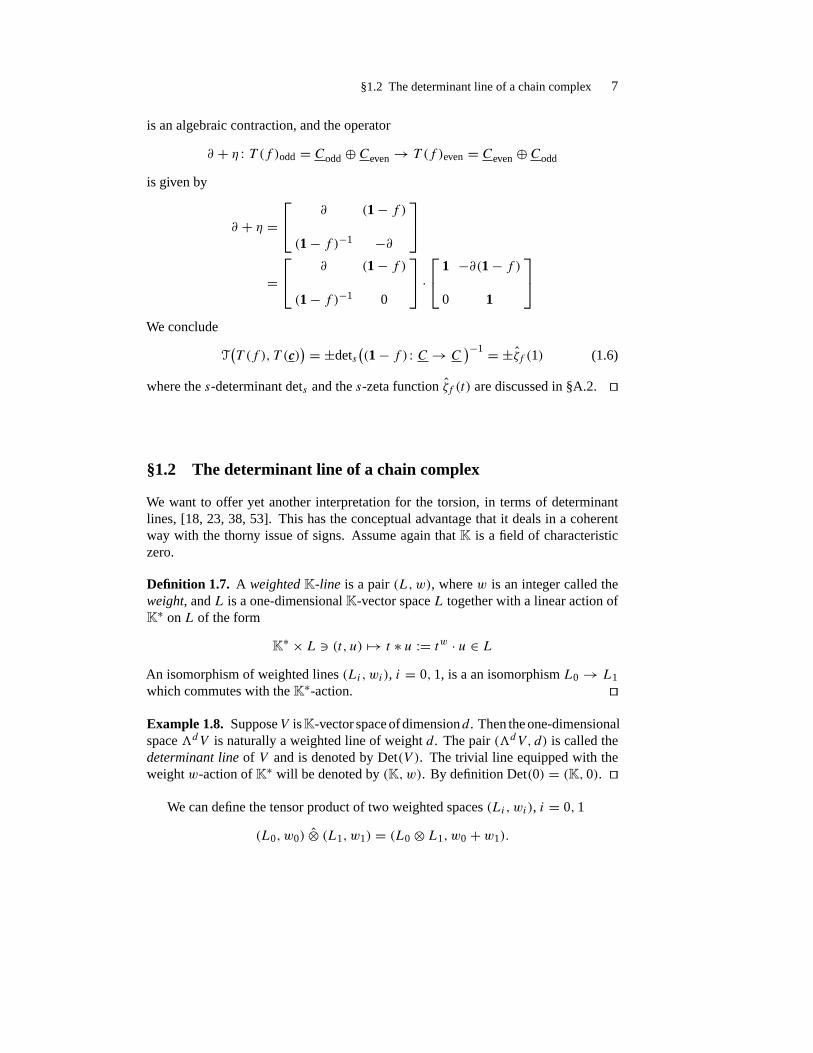
§1.2 The determinant line of a chain complex 7
is an algebraic contraction, and the operator
∂ + η : T (f )odd = Codd ⊕ Ceven → T (f )even = Ceven ⊕ Codd
is given by
∂ + η = ∂ (1− f )
(1− f )−1 −∂
= ∂ (1− f )
(1− f )−1 0
· 1 −∂(1− f )
0 1
We conclude
T(T (f ), T (c)
) = ±dets((1− f ) : C → C
)−1 = ±ζf (1) (1.6)
where the s-determinant dets and the s-zeta function ζf (t) are discussed in §A.2. �
§1.2 The determinant line of a chain complex
We want to offer yet another interpretation for the torsion, in terms of determinantlines, [18, 23, 38, 53]. This has the conceptual advantage that it deals in a coherentway with the thorny issue of signs. Assume again that K is a field of characteristiczero.
Definition 1.7. A weighted K-line is a pair (L,w), where w is an integer called theweight, and L is a one-dimensional K-vector space L together with a linear action ofK∗ on L of the form
K∗ × L � (t, u) → t ∗ u := tw · u ∈ LAn isomorphism of weighted lines (Li, wi), i = 0, 1, is a an isomorphism L0 → L1which commutes with the K∗-action. �
Example 1.8. SupposeV isK-vector space of dimensiond. Then the one-dimensionalspace �dV is naturally a weighted line of weight d. The pair (�dV, d) is called thedeterminant line of V and is denoted by Det(V ). The trivial line equipped with theweight w-action of K∗ will be denoted by (K, w). By definition Det(0) = (K, 0). �
We can define the tensor product of two weighted spaces (Li, wi), i = 0, 1
(L0, w0) ⊗ (L1, w1) = (L0 ⊗ L1, w0 + w1).

8 1 Algebraic preliminaries
The dual of a weighted line (L,w) is the weighted line
(L,w)−1 := (L∗,−w).
We can organize the collection of weighted lines as a category where
Hom((L0, w0), (L1, w1)) ={
0 if w0 �= w1
Hom(L0, L1) if w0 = w1.
Remark 1.9 (Koszul’s sign conventions). We would like to discuss an ubiquitous butquite subtle problem concerning signs. Suppose (Li, wi), i = 0, 1, are weighted lines.The tensor products
U = L0 ⊗ L1 and V = L1 ⊗ L0
are not equal as sets but are isomorphic as vector spaces. We will identify them, butnot using the obvious isomorphism. We well use instead the Koszul transposition
ϒL0,L1 : U → V, �0 ⊗ �1 → (−1)w0w1�1 ⊗ �0.
Similarly, given a weighted line (L,w), we will identify the tensor product (L,w)−1⊗(L,w) with Det(0) using in place of the obvious pairing, the Koszul contractionTrL : (L,w)−1 ⊗ (L,w)→ Det(0) defined by
L⊗ L∗ � (u, u∗) → u∗ u := (−1)w(w−1)/2〈u∗, u〉 ∈ K,
where 〈•, •〉 : L∗ × L→ K denotes the canonical pairing.Note that (L−1)−1 �= L but we will identify them using the tautological map
ıL : L←→ (L−1)−1.
The identifications ϒL0,L1 , TrL and ıL are compatible in the sense that the diagrambelow is commutative.
(L−1)−1 ⊗ L−1L ⊗ L−1 L−1 ⊗ L
Det(0).
�ıL⊗1
�����TrL−1
�ϒL,L−1
������ TrL
Finally note that L0 ⊗ (L1 ⊗ L2) �= (L0 ⊗ L1) ⊗ L2 but we will identify them viathe tautological isomorphism
L0 ⊗ (L1 ⊗ L2)→ (L0 ⊗ L1) ⊗ L2, �0 ⊗ (�1 ⊗ �2) → (�0 ⊗ �1)⊗ �2.

§1.2 The determinant line of a chain complex 9
The tautological identification (L0 ⊗ L1)−1 ı←→ L−1
0 ⊗ L−11 is compatible with the
above rules in the sense that the diagram below is commutative.
(L−10 ⊗L−1
1 )⊗(L0⊗L1)
(L0⊗L1)−1⊗(L0⊗L1) (L−1
0 ⊗L0)⊗(L−11 ⊗L1)
Det(0) .
�������ϒL−11 ,L0
��������TrL0⊗L1
�������ı⊗1
�������� TrL0 ⊗TrL1
To simplify the presentation we will use the following less accurate descriptions ofthe above rules.
L0 ⊗L1 = (−1)w0w1L1 ⊗L1, L−1 ⊗L = (−1)w(w−1)/2 Det(0), (L−1)−1 = L(L0 ⊗ L1) ⊗ L2 = L0 ⊗ (L1 ⊗ L2), (L0 ⊗ L1)
−1 = L−10 ⊗ L−1
1 .
Two weighted lines U , V are said to be equal up to permutation, and we write thisU =p V , if there exist weighted lines (Li, wi), i = 1, . . . , n and a permutation
ϕ : {1, . . . , n} → {1, . . . , n}such that
U =⊗n
i=1Li, V =
⊗n
i=1Lϕ(i).
We denote by ϒ = ϒϕ the composition of Koszul transpositions which maps U to V .We can generalize the Koszul contraction to the following more general context.
Suppose for example that (Li, wi), i = 0, 1, 2, 3, are weighted lines. Then define
Tr : U := L1 ⊗ L∗0 ⊗ L2 ⊗ L0 ⊗ L3 → V := L1 ⊗ L2 ⊗ L3,
u1 ⊗ u∗0 ⊗ u2 ⊗ u0 ⊗ u3 → (−1)w0w2(u∗0 u0) · u0 ⊗ u2 ⊗ u3.
This contraction continues to be compatible with the Koszul transpositions in thefollowing sense. For any permutation ϕ of the five factors
L1, L∗0, L2, L0, L3
we get a new line ϒϕ(U) equipped as above with a trace
Tr : ϒϕ(U)→ V
and the diagram below is commutative
U ϒϕ(U)
V .
�ϒϕ
����
Tr�
��� Tr
�
10 1 Algebraic preliminaries
Example 1.10. Suppose that Li , i = 0, 1 are weighted lines with the same weight wand u ∈ L−1
0 ⊗L1 is a nontrivial element. Then u defines an element in Hom(L0, L1)
u0 → u u1.
If u = u∗0 ⊗ u1 then
u u0 = (−1)w(w+1)/2〈u∗0, u0〉u1. � IfW∗ =⊕j∈ZWj is a finite dimensional Z-graded K-vector space then its deter-
minant line is the weighted line
Det(W) =⊗
j∈ZDet(W−j )(−1)j .
Its weight is the Euler characteristic
χ(W) =∑j∈Z
(−1)j dimWj .
For example, ifW = W0 ⊕W1 ⊕W2, then
Det(W) = Det(W2) ⊗ Det(W1)−1 ⊗ Det(W0).
To perform numerical computations we need to work with richer objects, namelybased vector spaces and based weighted lines. All the tensorial operations on vectorspaces have a based counterpart. The dual of a based vector space (W,w) is thebased vector space (W ∗,w∗), where w∗ denotes the dual basis. The dual of a basedweighted line (L,w, δ) is the based weighted line (L,w, δ)−1 := (L∗,−w, δ∗)whereδ∗ denotes the basis of L∗ dual to δ,
〈δ∗, δ〉 = 1.
We can define the ordered tensor product of based weighted lines
(L0, w0, δ0) ⊗ (L1, w1, δ1) = (L0 ⊗ L1, w0 + w1, δ0 ∧ δ1).To any based vector space (W,w) we can associate in a tautological fashion a basedweighted line (Det(W), dimW, det w). If
(W,w) =⊕n∈Z
(Wn,wn)
is a based graded vector space, the associated based determinant line is
(Det(W), χ(W), det w) =⊗(
Det(W−n), dimW−n, det w−n)(−1)n
.
Given two based weighted lines (Li, wi, δi), i = 0, 1, and a morphismf : (L0, w0)→(L1, w1) we define its torsion to be the scalar 〈δ1|f |δ0〉 ∈ K uniquely determined bythe equality
f (δ0) = 〈δ1|f |δ0〉δ1.
§1.2 The determinant line of a chain complex 11
Example 1.11. Suppose W = ⊕n∈ZWn is a finite dimensional Z-graded K-vectorspace, dn := dimKWn. Define
Det+(W) :=⊗n∈Z
Det(W−2n), Det−(W) :=⊗n∈Z
Det(W−2n−1),
Dets (W) = Det+(W) ⊗ Det−(W)−1 =p Det(W).
For example, ifW = W0 ⊕W1 ⊕W2 then
Dets(W) = Det(W2) ⊗ Det(W0) ⊗ Det(W1)−1
= (−1)d0d1 Det(W) = (−1)d0d1 Det(W2)⊗ Det(W1)−1 ⊗ Det(W0). �
We have the following important result.
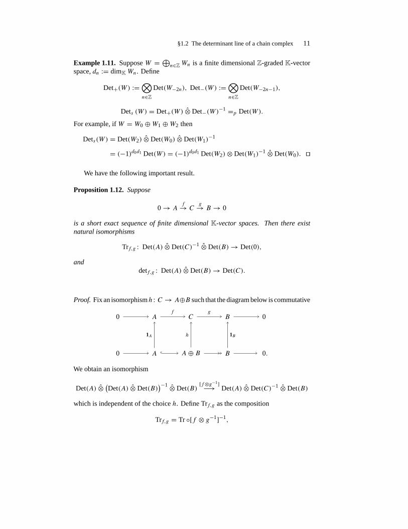
Proposition 1.12. Suppose
0 → Af→ C
g→ B → 0
is a short exact sequence of finite dimensional K-vector spaces. Then there existnatural isomorphisms
Trf,g : Det(A) ⊗ Det(C)−1 ⊗ Det(B)→ Det(0),
anddetf,g : Det(A) ⊗ Det(B)→ Det(C).
Proof. Fix an isomorphismh : C → A⊕B such that the diagram below is commutative
0 A C B 0
0 A A⊕ B B 0.
� �f �g �
�
�1A
� �
�h
��
�1B
�We obtain an isomorphism
Det(A) ⊗ (Det(A) ⊗ Det(B))−1 ⊗ Det(B)
[f⊗g−1]−→ Det(A) ⊗ Det(C)−1 ⊗ Det(B)
which is independent of the choice h. Define Trf,g as the composition
Trf,g = Tr ◦[f ⊗ g−1]−1,
12 1 Algebraic preliminaries
i.e.
Det(A) ⊗ (Det(A) ⊗ Det(B))−1 ⊗ Det(B)
Det(A) ⊗ Det(C)−1 ⊗ Det(B) Det(0),�
[f⊗g−1]���������
Tr
�Trf,g
where the map
Tr : Det(A) ⊗ (Det(A) ⊗ Det(B))−1 ⊗ Det(B)→ Det(0)
is the Koszul contraction. By taking tensor products we obtain an isomorphism
Det(A) ⊗ Det(C)−1 ⊗ Det(B) ⊗ Det(C)→ Det(C),
and if we take the Koszul contraction on the left hand side we obtain another isomor-phism
Det(A) ⊗ Det(B)Tr←− Det(A) ⊗ Det(C)−1 ⊗ Det(B) ⊗ Det(C)
The definition of detf,g is now obvious. �
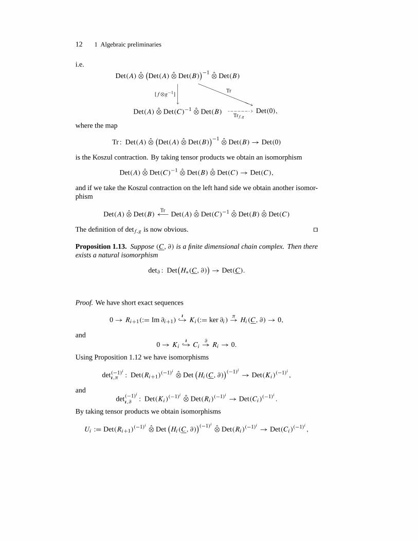
Proposition 1.13. Suppose (C, ∂) is a finite dimensional chain complex. Then thereexists a natural isomorphism
det∂ : Det(H∗(C, ∂)
)→ Det(C).
Proof. We have short exact sequences
0 → Ri+1(:= Im ∂i+1)ı↪→ Ki(:= ker ∂i)
π→ Hi(C, ∂)→ 0,
and0 → Ki
ı↪→ Ci
∂→ Ri → 0.
Using Proposition 1.12 we have isomorphisms
det(−1)iı,π : Det(Ri+1)
(−1)i ⊗ Det(Hi(C, ∂)
)(−1)i → Det(Ki)(−1)i ,
anddet(−1)i
ı,∂ : Det(Ki)(−1)i ⊗ Det(Ri)
(−1)i → Det(Ci)(−1)i .
By taking tensor products we obtain isomorphisms
Ui := Det(Ri+1)(−1)i ⊗ Det
(Hi(C, ∂)
)(−1)i ⊗ Det(Ri)(−1)i → Det(Ci)
(−1)i ,

§1.2 The determinant line of a chain complex 13
and
[det ∂] :⊗∞
−n=−∞Un→ Det(C).
Taking the Koszul contractions of the pairs (R−1i , Ri) in the left-hand-side we obtain
an isomorphismTr : L→ Det
(H∗(C, ∂)
).
Then det∂ is the unique isomorphism which renders commutative the diagram below.
L
Det(H∗(C, ∂)
)Det(C).
�����[det ∂]�����
Tr
�det∂ �
Definition 1.14. The inverse of the above isomorphism is known as the Euler isomor-phism and will be denoted by EulC = Eul(C,∂). �
Example 1.15. Consider the elementary complex
0 ↪→ C1 = V 1V→ V = C0 → 0
Then the Euler isomorphism
Det(V )−1 ⊗ Det(V )→ Det(0)
coincides with the Koszul contraction. This simple fact lies at the core of the remark-able compatibility between the Euler isomorphism and the various Koszul identifica-tions, and keeps in check what Deligne called in [18] “le cauchemar de signes”. �
Example 1.16. Suppose that (C, c, ∂) is a finite dimensional acyclic complex. Wecan choose as in the previous section linearly ordered finite collections bi ⊂ Ci suchthat the restriction of ∂ to the span of bi is one-to-one, and the linearly ordered set∂bi+1 ∪ bi is a basis of Ci . We then get a basis
δ := · · · ∧ (det ∂bi+1 ∧ det bi)(−1)i ∧ (det ∂bi ∧ bi−1
)(−1)i−1 ∧ · · · ∈ Det(C).
The Euler isomorphism maps Det(C) to Det(0), and the basis δ to the canonical basis(−1)ν of Det(0), where
ν =n∑i=1
|bi |(|bi | + (−1)i)
2.
�
14 1 Algebraic preliminaries
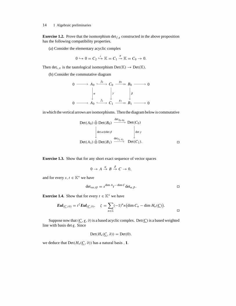
Exercise 1.2.Prove that the isomorphism detf,g constructed in the above propositionhas the following compatibility properties.
(a) Consider the elementary acyclic complex
0 ↪→ 0 = C2ι↪→ K = C1
π� K = C0 → 0.
Then detι,π is the tautological isomorphism Det(K)→ Det(K).
(b) Consider the commutative diagram
0 A0 C0 B0 0
0 A0 C1 B1 0
� � �f0
�α
�γ
��g0
�β
�
� � �f1 ��g1 �in which the vertical arrows are isomorphisms. Then the diagram below is commutative
Det(A0) ⊗ Det(B0) Det(C0)
Det(A1) ⊗ Det(B1) Det(C1).
�detf0,g0
�det α⊗det β
�det γ
�detf1,g1 �
Exercise 1.3.Show that for any short exact sequence of vector spaces
0 → Aα→ B
β→ C → 0,
and for every s, t ∈ K∗ we have
detsα,tβ = sdimAt− dimCdetα,β . �
Exercise 1.4.Show that for every t ∈ K∗ we have
Eul(C,t∂) = tζEul(C,∂), ζ =∑n∈Z
(−1)nn(dimCn − dimHn(C)
).
�
Suppose now that (C, c, ∂) is a based acyclic complex. Det(C) is a based weightedline with basis det c. Since
Det(H∗(C, ∂)) = Det(0).
we deduce that Det(H∗(C, ∂)) has a natural basis ,1.

§1.2 The determinant line of a chain complex 15
Proposition 1.17.T(C, c) = (−1)ν
⟨1∣∣EulC
∣∣ det c⟩.
where ν is defined as in Example 1.16.
Exercise 1.5.Prove the above equality. �
WhenK = Rwe can be even more explicit. More precisely, fix Euclidean metricson each of Ci . Then, as explained in §A.1, we can explicitly write down a generalizedcontraction (Definition A.7), i.e. a degree one map
η : Ck → Ck+1
such that η2 = 0 andP = ∂η+η∂ = (∂+η)2 is a projector onto a perfect subcomplexwith the same homology as C. More precisely, we can choose η of the form
η = (ii∗ +�)−1∂∗
where� = (∂+∂∗)2, and i is the natural inclusion i : ker�→ C. The formal Hodgetheorem shows that ker� ∼= H∗(C). Consider the linear operator
ker�odd ⊕ Ceven → ker�even ⊕ Codd,
[koddceven
]→[
0 i∗eveniodd ∂ + η
]·[koddceven
].
We thus get an isomorphism
Det ker�odd ⊗ Det(Ceven)→ Det ker�even ⊗ Det(Codd)
This yields the isomorphisms
Det ker�odd ⊗ Dets (C)→ Det ker�even,
and
I : Dets (C)→ Det(ker�odd)−1 ⊗ Det ker�even → Dets
(H∗(C)
).
Up to a permutation, this is the Euler isomorphism. More precisely, we have a com-mutative diagram
Dets (C) Dets(H∗(C)
)
Det(C) Det(H∗(C)
).
�I
�ϒ
�ϒ
�EulC

16 1 Algebraic preliminaries
§1.3 Basic properties of the torsion
The torsion behaves nicely with respect to the basic operations on chain complexes.Consider first a short exact sequence of chain complexes
0 → (A, ∂A)f→ (C, ∂C)
g→ (B, ∂B)→ 0.
Using Proposition 1.12 we obtain canonical isomorphisms
detfn,gn ∈ Det(An) ⊗ Det(Bn)→ Det(Cn),
and thus an isomorphism
detf,g :⊗∞
n=−∞(Det(An) ⊗ Det(Bn)
)(−1)n → Det(C).
Now observe that⊗∞−n=−∞
(Det(An) ⊗ Det(Bn)
)(−1)n =p Det(A) ⊗ Det(B).
We get an isomorphism
detf,g : Det(A) ⊗ Det(B)→ Det(C)
compatible with the Koszul permutation identifying the two weighted lines,
Det(A) ⊗ Det(B),⊗∞
−n=−∞(Det(An) ⊗ Det(Bn)
)(−1)n.
On the other hand, we have a long exact sequence
· · · ∂→ Hq(A)f∗→ Hq(C)
g∗→ Hq(B)∂→ Hq−1(A)→ · · · .
We can regard this sequence as an acyclic complex which we denote by H(A,B,C).The Euler isomorphism of this acyclic complex induces an isomorphism
EulH(A,B,C) : Det(H(A,B,C))→ Det(0).
Taking the tensor product of Det(H(A,B,C)) with Det(H∗(C)) and then applyingthe Koszul contraction to the pair
Det(H∗(C))−1, Det(H∗(C))
we obtain an isomorphism
H(detf,g) : Det(H∗(A)) ⊗ Det(H∗(B))→ Det(H∗(C)).

§1.3 Basic properties of the torsion 17
Proposition 1.18. The diagram below is commutative.
Det(A) ⊗ Det(B) Det(C)
Det(H∗(A)
) ⊗ Det(H∗(B)
)Det(H∗(C)
).
�detf,g
�EulA⊗EulB
�EulC
�H(detf,g)
(1.7)
To better understand the meaning of the above result suppose we fix bases a, b, c
of A, B and respectively C, and bases [a], [b], [c] of H∗(A), H∗(B) and respectivelyH∗(C). We assume that
c = f (a) ∪ b′, g(b′) = b.
We can now identify EulA, EulB , EulC with scalars in K∗. H(detf,g) can also beidentified with a scalar, the torsion of the acyclic complex H(A,B,C). Then (1.7)implies
EulC ·T−1H(A,B,C) = ±EulA ·EulB . (1.8)
Exercise 1.6.Prove (1.7) and (1.8). �
The above result implies immediately that the torsion is multiplicative with respectto direct sums. More precisely, we have the following elementary, but extremelyversatile result.
Theorem 1.19. Consider a short exact sequence of, based acyclic complexes of K-vector spaces
0 → (A, a)f→ (C, c)
g→ (B, b)→ 0,
such thatc = f (a) ∪ b′, g(b′) = b.
Then H(detf,g) = 1, ⟨det c|detf,g| det a ⊗ det b
⟩ = ±1,
and ⟨1|EulA | det a
⟩ · ⟨1|EulB | det b⟩ = ⟨1|EulC | det c
⟩ · ⟨det c|detf,g|a ⊗ b⟩.
In particular,T(C, c) = ±T(A, a) · T(B, b).

18 1 Algebraic preliminaries
For any chain complex (C, ∂) and any k ∈ Z we denote by (C[k], ∂) the degreeshifted complex defined by
C[k]i = Ci+k, ∀i ∈ Z.Observe that
Det(C[k]) =p Det(C)(−1)k ,
and we have a commutative diagram
Det(C[k]) (Det(C)
)(−1)k
Det(H∗+k(C)
) (DetH∗(C)
)(−1)k.
�Koszul
�EulC[k]
�Eul (−1)k
C
�Koszul
Given a chain complex
(C, ∂) =⊕j∈Z
(Cj , ∂j )
of K-vector spaces we can form its dual C− defined by
C−j := C∗−j := Hom(C−j ,K),
and whose boundary maps are the duals of the boundary maps of C. We have acommutative diagram
Det(C−) ⊗ Det(C) Det(H∗(C−1)
) ⊗ Det(H∗(C)
)Det(0).
�������Tr
�EulC− ⊗EulC
������ Tr
In particular, if C is acyclic, and c is a basis, then
T(C, c) · T(C−, c−) = ±1, (1.9)
where c−n = c∗−n. Suppose now that the field K is equipped with an involutiveautomorphism
ε : K→ K.
Example 1.20. IfK = C we can take ε to be the complex conjugation. IfK = Q(t),the field of rational functions in one variable, then the correspondence t → t−1 inducessuch an involution. �

§1.3 Basic properties of the torsion 19
The ε-conjugate of a K-vector space V is the vector space V = V ε which coincideswith V as an Abelian group while the scalar multiplication is given by
K× V � (λ, v) → ε(λ)v.
We denote by ε = εV : V → V ε the tautological bijection. A linear map A : U → V
tautologically induces a linear map Aε : U ε → V ε.An ε-pairing between the K-vector spaces U , V is a bilinear map
〈•, •〉 : U × V ε → K.
Observe that such a pairing induces a K-linear map
T : V ε → U∗, v → 〈•, v〉.
The K-pairing is called perfect (or a duality) if the induced K-linear map
T : V ε → U∗
is an isomorphism. If U , V happen to be Z2-graded
U ∼= U+ ⊕ U−, V = V+ ⊕ V−then the duality is called supersymmetric if the operator T is supersymmetric, i.e. itis either purely odd, T (V ε±) = U∗∓, or purely even, T (V ε±) = U∗±. Correspondingly,a supersymmetric duality can be even or odd. We will denote by ν the parity of asupersymmetric duality.
Consider the length n chain complexes of C = ⊕ni=0Ci and D = ⊕nj=0Dj ofK-vector spaces with ambiguities A. A chain complex pairing is a pairing
〈•, •〉 : C × Dε → K
such that the induced map T is a degree zero morphism between the chain complexes
T : Dε → C−[n].
Observe that such pairings are supersymmetric with respect to the naturalZ2-gradingson the chain complexes. The parity of the pairing is the same as the parity of n- thelength of the chain complexes. A pairing is called perfect if the induced morphism isan isomorphism. We have the following immediate result.
Proposition 1.21(Abstract duality theorem). Suppose
〈•, •〉 : C × Dε → K
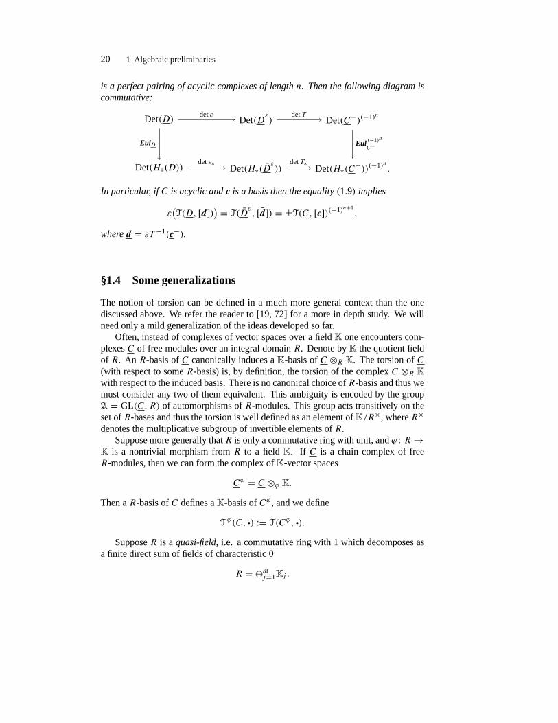
20 1 Algebraic preliminaries
is a perfect pairing of acyclic complexes of length n. Then the following diagram iscommutative:
Det(D) Det(Dε) Det(C−)(−1)n
Det(H∗(D)) Det(H∗(Dε)) Det(H∗(C−))(−1)n .
�EulD
�det ε �det T
�Eul (−1)n
C−
�det ε∗ �det T∗
In particular, if C is acyclic and c is a basis then the equality (1.9) implies
ε(T(D, [d])) = T(D
ε, [d]) = ±T(C, [c])(−1)n+1
,
where d = εT −1(c−).
§1.4 Some generalizations
The notion of torsion can be defined in a much more general context than the onediscussed above. We refer the reader to [19, 72] for a more in depth study. We willneed only a mild generalization of the ideas developed so far.
Often, instead of complexes of vector spaces over a field K one encounters com-plexes C of free modules over an integral domain R. Denote by K the quotient fieldof R. An R-basis of C canonically induces a K-basis of C ⊗R K. The torsion of C(with respect to some R-basis) is, by definition, the torsion of the complex C ⊗R Kwith respect to the induced basis. There is no canonical choice ofR-basis and thus wemust consider any two of them equivalent. This ambiguity is encoded by the groupA = GL(C,R) of automorphisms of R-modules. This group acts transitively on theset of R-bases and thus the torsion is well defined as an element of K/R×, where R×denotes the multiplicative subgroup of invertible elements of R.
Suppose more generally that R is only a commutative ring with unit, and ϕ : R→K is a nontrivial morphism from R to a field K. If C is a chain complex of freeR-modules, then we can form the complex of K-vector spaces
Cϕ = C ⊗ϕ K.Then a R-basis of C defines a K-basis of Cϕ , and we define
T ϕ(C, •) := T(Cϕ, •).
Suppose R is a quasi-field, i.e. a commutative ring with 1 which decomposes asa finite direct sum of fields of characteristic 0
R = ⊕mj=1Kj .

§1.5 Abelian group algebras 21
Denote by ϕj the natural projection R → Kj . Suppose C is a chain complex of free,R-modules. A R-basis c of C induces a Kj -basis of Cϕj and as above we obtain atorsion
T ϕj (C, [c]A) ∈ K∗j / det A ∪ {0}.The direct sum
m⊕j=1
T ϕj (C, [c]A) ∈(⊕jKj )/ det A
is an element in R/ det A – the space of orbits of the determinant action of A on R.We can further extend the class of coefficient rings to include the quasi-integral
domains, i.e. the commutative ringsR with 1 such that the associated ring of fractionsQ(R) (i.e. the localization with respect to the prime ideal of zero divisors) is a quasi-field
Q(R) = ⊕jKj .Denote by ϕj : R → Kj the natural morphism. If C is a chain complex of free,R-modules then, by definition, its torsion is the direct sum
T(C, •) :=⊕j
T ϕj (C, •) ∈ Q(R)/ det A.
Let us observe the following simple fact.
Proposition 1.22. Suppose R is a quasi-integral domain of characteristic zero, K isa field of characteristic zero and ϕ : R→ K is a nontrivial morphism. If C is a chaincomplex of free R-modules then
ϕ(T(C, •)
) = T ϕ(C, •).
§1.5 Abelian group algebras
In this section we want to describe a few special features of the group algebras offinitely generated Abelian groups since they will play a central role in topologicalapplications.
Suppose H is a finitely generated Abelian group. It can be non-canonically de-composed as
H = FH ⊕ Tors(H),
where FH denotes the free part of H , FH ∼= H/Tors(H). Denote by Q(H) the ringof fractions of the group algebra Z[H ].
Proposition 1.23. Z[H ] is a quasi-integral domain of characteristic zero.
22 1 Algebraic preliminaries
Proof. Let us first consider the two extremes, Tors(H) = 0, or FH = 0.
• If Tors(H) = 0 thenH = FH , and if rankH = n, thenQ(H) is the field of rationalfunctions in n variables with rational coefficients.
• If FH = 0, so thatH = Tors(H), thenQ[H ] is a semisimple, commutative algebra,and thus decomposes as a sum of fields; see [55]. In particular, Q[H ] = Q(H).
In general we have
Q[H ] = Q[Tors(H)][FH ] ∼=⊕i
Ki[FH ],
where the summands Ki are the fields entering into the direct sum decomposition ofQ[Tors(H)]. Thus,
Q(Z[H ]) = Q(H) =⊕i
Ki (FH ).
Each of the above summands is a field of rational functions in n = rank(H) variables.�
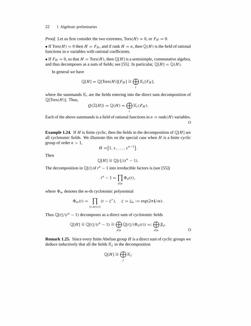
Example 1.24. If H is finite cyclic, then the fields in the decomposition of Q[H ] areall cyclotomic fields. We illustrate this on the special case when H is a finite cyclicgroup of order n > 1,
H ={1, x, . . . , xn−1}.Then
Q[H ] ∼= Q[t]/(tn − 1).
The decomposition in Q[t] of tn − 1 into irreducible factors is (see [55])
tn − 1 =∏d|n�d(t),
where �m denotes the m-th cyclotomic polynomial
�m(t) =∏
(r,m)=1
(t − ζ r ), ζ = ζm := exp(2π i/m).
Thus Q[t]/(tn − 1) decomposes as a direct sum of cyclotomic fields
Q[H ] ∼= Q[t]/(tn − 1) ∼=⊕d|nQ[t]/(�d(t)) =:
⊕d|n
Fd .�
Remark 1.25. Since every finite Abelian groupH is a direct sum of cyclic groups wededuce inductively that all the fields Kj in the decomposition
Q[H ] ∼=⊕j
Kj
§1.5 Abelian group algebras 23
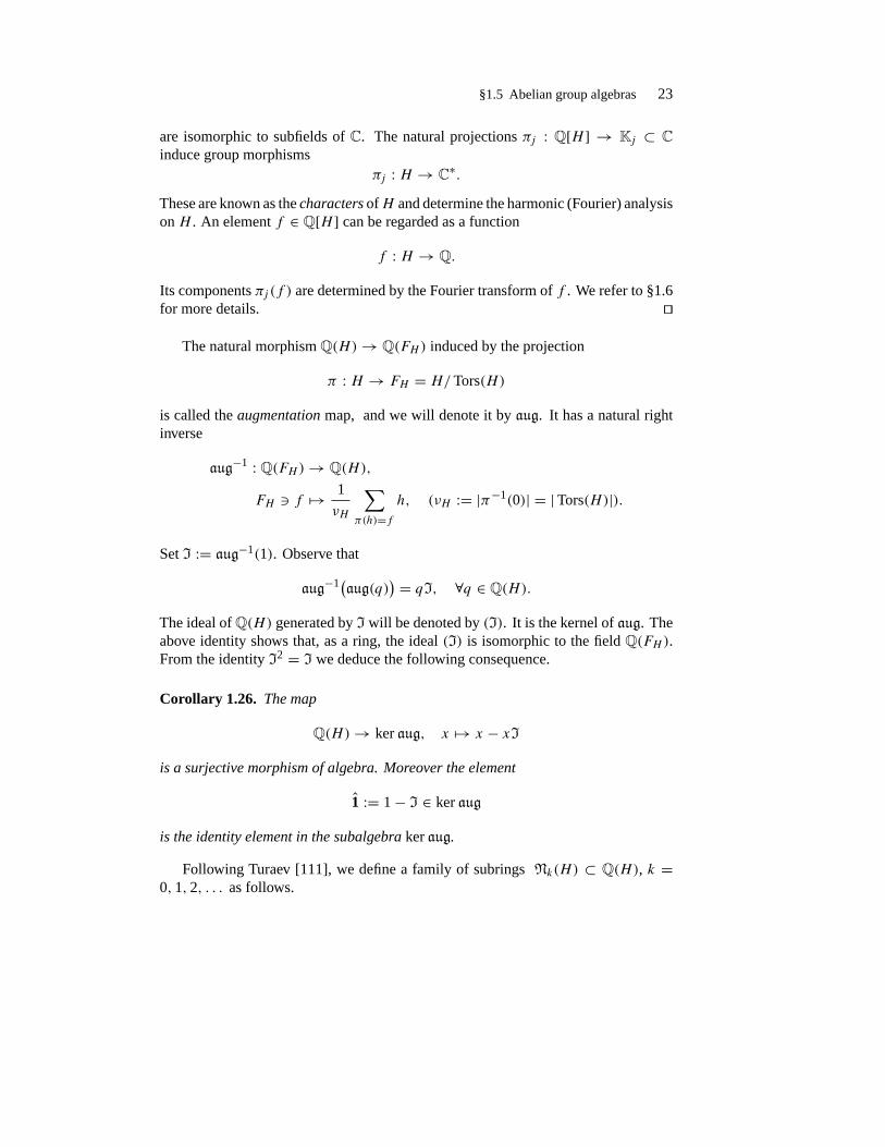
are isomorphic to subfields of C. The natural projections πj : Q[H ] → Kj ⊂ Cinduce group morphisms
πj : H → C∗.
These are known as the characters ofH and determine the harmonic (Fourier) analysison H . An element f ∈ Q[H ] can be regarded as a function
f : H → Q.
Its components πj (f ) are determined by the Fourier transform of f . We refer to §1.6for more details. �
The natural morphism Q(H)→ Q(FH ) induced by the projection
π : H → FH = H/Tors(H)
is called the augmentation map, and we will denote it by aug. It has a natural rightinverse
aug−1 : Q(FH )→ Q(H),
FH � f → 1
νH
∑π(h)=f
h, (νH := |π−1(0)| = |Tors(H)|).
Set I := aug−1(1). Observe that
aug−1(aug(q)) = qI, ∀q ∈ Q(H).
The ideal ofQ(H) generated by I will be denoted by (I). It is the kernel of aug. Theabove identity shows that, as a ring, the ideal (I) is isomorphic to the field Q(FH ).From the identity I2 = I we deduce the following consequence.
Corollary 1.26. The map
Q(H)→ ker aug, x → x − xIis a surjective morphism of algebra. Moreover the element
1 := 1− I ∈ ker aug
is the identity element in the subalgebra ker aug.
Following Turaev [111], we define a family of subrings Nk(H) ⊂ Q(H), k =0, 1, 2, . . . as follows.

24 1 Algebraic preliminaries
A. If rank(H) ≥ 1 then
N0(H) := Z[H ],Nk(H) = {q ∈ Q(H); (1− h)q ∈ Nk−1(H),∀h ∈ H }.
Roughly speaking, Nk(G) consists of all solutions in x ∈ Q(G) of the linear system
(1− g)kx ∈ Z[G], ∀g ∈ G.B. If rank(H) = 0 then
Nk(H) = ker aug ⊂ Q(H), ∀k = 0, 1, . . . .
Observe thatN0(H) ⊂ N1(H) ⊂ · · · ⊂ Nk(H) ⊂ · · · .
We setN(H) = lim
k→∞Nk(H),
S := νHI =∑
u∈Tors(H)
u ∈ Z[H ], νH = |Tors(H)|.
Proposition 1.27([111]). Let H be a finitely generated Abelian group of rank ≥ 1.
(a) If rank(H) ≥ 2 then Nk(H) = Z[H ], ∀k = 0, 1, 2, . . . .
(b) Suppose rank(H) = 1. Denote by t a generator of F := H/Tors(H) and setT = aug−1(t). Then
x ∈ Nk(H) = Z[H ] +SZ[H ](1− T )−k.
Proof. (a) It suffices to prove N1(H) = N0(H). The equality is obvious if H istorsion free. Suppose now Tors(H) �= 0. Any x ∈ Q(H) decomposes uniquely as
x := x + x⊥
wherex := Ix = aug−1aug(x), x⊥ := (1− I)x.
Suppose x ∈ Q(H) is such that
(1− h)x ∈ Z[H ], ∀h ∈ H.Observe that aug(x) ∈ N1(H/Tors(H)) = Z[H/Tors(H)] so that
x = aug−1aug(x) ∈ IZ[H ].
§1.5 Abelian group algebras 25
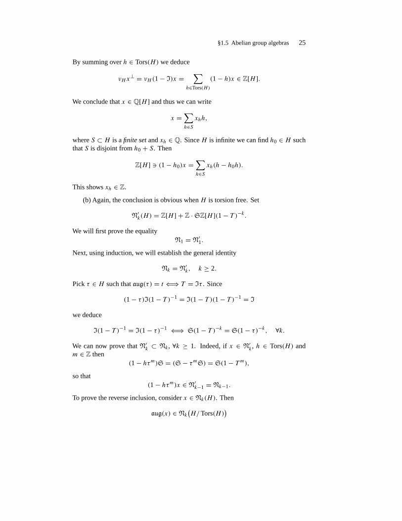
By summing over h ∈ Tors(H) we deduce
νHx⊥ = νH (1− I)x =
∑h∈Tors(H)
(1− h)x ∈ Z[H ].
We conclude that x ∈ Q[H ] and thus we can write
x =∑h∈Sxhh,
where S ⊂ H is a finite set and xh ∈ Q. Since H is infinite we can find h0 ∈ H suchthat S is disjoint from h0 + S. Then
Z[H ] � (1− h0)x =∑h∈Sxh(h− h0h).
This shows xh ∈ Z.
(b) Again, the conclusion is obvious when H is torsion free. Set
N′k(H) = Z[H ] + Z ·SZ[H ](1− T )−k.
We will first prove the equalityN1 = N′
1.
Next, using induction, we will establish the general identity
Nk = N′k, k ≥ 2.
Pick τ ∈ H such that aug(τ ) = t ⇐⇒ T = Iτ . Since
(1− τ)I(1− T )−1 = I(1− T )(1− T )−1 = I
we deduce
I(1− T )−1 = I(1− τ)−1 ⇐⇒ S(1− T )−k = S(1− τ)−k, ∀k.We can now prove that N′
k ⊂ Nk , ∀k ≥ 1. Indeed, if x ∈ N′k , h ∈ Tors(H) and
m ∈ Z then(1− hτm)S = (S− τmS) = S(1− T m),
so that(1− hτm)x ∈ N′
k−1 = Nk−1.
To prove the reverse inclusion, consider x ∈ Nk(H). Then
aug(x) ∈ Nk(H/Tors(H)
)

26 1 Algebraic preliminaries
so that
x = Ix = aug−1aug(x) ∈ IZ[τ ] + IZ[τ ](1− τ)−k = 1
νHSZ[H ](1− τ)−k.
Summing the congruences (1− h)x ∈ Nk−1(H) over h ∈ Tors(H) we deduce
νHx⊥ ∈ Nk−1(H) = Z[H ] +SZ[H ](1− T )−(k−1).
Thus
x ∈ 1
νH
(Z[H ] +SZ[H ](1− T )−k)
and(1− h)x ∈ Z[H ] +SZ[H ](1− τ)−(k−1), ∀h ∈ H.
We writex⊥ = A, x = SB(1− τ)−k.
We need to consider two cases.
A. k = 1. In this case
x⊥ = A ∈ 1
νHZ[H ], x = SB(1− τ)−1 ∈ 1
νHSZ[H ](1− τ)−1,
and we can write
A =∑m∈Z
( ∑u∈Tors(H)
am,uu)τm, B =
∑m∈Z
( ∑u∈Tors(H)
bm,uu)τm.
Setbm =
∑u
bm,u.
ThenSB = S
∑m
bmτm.
Denote by αm,u (resp. βm) the image of am,u (resp. bm) in Q/Z. Observe that
νhβm = 0 = νHαm,u.Since (1− u)S = 0, ∀u ∈ Tors(H) we deduce
(1− u)x = (1− u)A ∈ Z[H ], ∀u ∈ Tors(H) ⇐⇒ αm,v = αm,u, (1.10)
∀u, v ∈ Tors(H), ∀m. Denote by αm the common value of αm,u, u ∈ Tors(H) andby km the integer 0 ≤ km < νH such that
km
νH= αm in Q/Z.

§1.5 Abelian group algebras 27
Define
K :=∑m
km
νHτm ∈ 1
νHSZ[H ].
The identities (1.10) can be rephrased in the following compact form,
A−SK ∈ Z[H ].On the other hand, the identities
(1− τ)x ∈ Z ⇐⇒ αm+1 − αm + βm+1 = 0, ∀mcan now be rewritten
S(1− τ)K +SB ∈ SZ[H ]so that
x = (A−SK)+S(B + (1− τ)K)(1− τ)−1 ∈ Z[H ] +SZ[H ](1− τ)−1 = N′
1.
B. k > 1. SetS := {h ∈ H ; ahbh �= 0}.
Then if h0 ∈ H is such that S ∩ (h0 + S) = ∅ and we conclude as in part (a). �
The above proposition has the following immediate consequence.
Corollary 1.28. Suppose that H is a finitely generated Abelian group. Denote byı : H → N(H) the natural morphism. If P,Q ∈ N(H) then
P |Q ⇐⇒ P |Q(ı(h)− 1), ∀h ∈ H.
Example 1.29. Suppose H ∼= Z⊕G whereG is a finite Abelian group. Denote by tthe generator of Z. Then
T = It = 1
NSt =
(1
N
∑g∈G
g
)t, N := |G|
The group algebra Q[H ] is isomorphic to the ring of Laurent polynomials
Q[H ] ∼= Q[G][t, t−1] ∼=⊕
Ki[t, t−1].Then
N[H ] = Z[H ] +SZ[T , T −1, (1− T )−1]. �
The correspondence H → N(H) is functorial. More precisely we have thefollowing result due to V. Turaev.

28 1 Algebraic preliminaries
Proposition 1.30([111]). Every epimorphism
f : H1 → H2
induces a morphism of Q-algebras f� : N(H1) → N(H2) such that the diagrambelow is commutative.
H1 H2
N(H1) N(H2).
�f
�ı1
�ı2
�f�
Proof. f� is defined as follows. Observe first that f induces a morphism
f∗ : Z[H1] → Z[H2] → N(H2).
If rank(H1) ≥ 2 then we set f� = f∗. If rank(H1) = 0 then f� denotes the restrictionof f∗ to ker aug ⊂ Q[H1].
When rank(H1) = 1 the definition is a bit more intricate. Denote by t a generatorof FH1 = H1/Tors(H1), choose τ ∈ H1 an element projecting to t and set T :=aug−1(t). We claim that there exists an unique X = Xf ∈ N(H2) such that
Xf∗(τ −1) = Xf∗(T −1) = f∗(S1), Xf∗(h−1) = 0, ∀h ∈ Tors(H1). (1.11)
Uniqueness. If X,X′ are two solutions of (1.11) then
(X −X′)f∗(u− 1) = 0, ∀u ∈ H1.
Since f : H1 → H2 is onto we deduce from Corollary 1.28 that X −X′ = 0.
Existence. Any element u ∈ H decomposes uniquely as
u = hτk, h ∈ TH1 , k ∈ Z.Then
f∗(S1)f∗(u− 1) = f∗(S1hτ −S1) = f∗(I1)f∗(τ k − 1).
Thusf∗(τ − 1)|f∗(u− 1)f∗(S1), ∀u ∈ H1.
Since f : H1 → H2 is surjective we deduce from Corollary 1.28
f∗(τ − 1)|f∗(S1) in N(H2).
Thus, there exists X1 ∈ N(H2) such that
f∗(S1) = X1f∗(τ − 1).

§1.5 Abelian group algebras 29
We then setXf := X1f∗(I1).
Finally, define f� = f∗ on Z[H ] and
f�(S1(T − 1)−1) := Xf . �
Remark 1.31. If H1f1→ H2
f2→ H3 is are epimorphisms of Abelian groups then
(f2 ◦ f1)� = (f2)� ◦ (f1)�.
Thus the correspondence G → N(G) defines a covariant functor from the categoryof finitely generated Abelian groups with epimorphisms as arrows to the category ofcommutativeQ-algebras. We refer to the next section for a more geometric descriptionof the morphism f� in terms of Fourier transform. �
Example 1.32. Suppose f is the natural projection Z→ Zn = Z/(nZ). Then
N(Z) ∼= Z[t, t−1, (1− t)−1], N(Zn) =(
1− 1
n
n∑j=1
sj)· Z[s], sn = 1.
Then f� is determined by
1 → 1= (1− I), t → (1− I)s, I = s(
1− 1
n
n∑j=1
sj).
Observe that(t − 1) → (s − 1)(1− I).
The inverse of (1− s) in the algebra ker aug with unit 1= 1− I is (see [81] or §1.6)
(1− s)−1 =(
12− d(s)
),
where
d(s) :=n∑k=1
((k
n
))sk,
and ((x)) is denotes Dedekind’s symbol
((x)) :={
0 x ∈ Zx − #x$ − 1
2 x ∈ R \ Z.(#x$ := the largest integer ≤ x.) �
30 1 Algebraic preliminaries
§1.6 Abelian harmonic analysis
When studying the torsion of a 3-manifold one is often lead to solving linear equationsof the form ax = b, where a, b belong to the group algebraC[G] of a finitely generatedAbelian group G. When G has torsion elements the ring Z[G] has zero divisors andthus the above equation may have more than one solution. Finding the annihilator of agiven elementa ∈ C[H ] is never an easy job due to the complexity of the multiplicationoperation in this algebra. This complexity is only artificial and magically disappears ifwe perform a simple but extremely versatile trick, namely taking the Fourier transformof the above equation. In the Fourier picture the above equation simplifies dramaticallyto the point that it can be solved explicitly.
The versatility of the Fourier transform can be very clearly seen in the very simpledescription of the rings N(G) and morphisms f� introduced in the previous section.These rings are essentially described in terms of linear equations in the ring Z[G].More precisely, N(G) is obtained by adjoining to Z[G] certain solutions x ∈ Q(G)of the family of linear equations linear equations
(1− g)k · x = f, g ∈ G, f ∈ Z[G].The Fourier transform fits these equations like a glove. The goal of the present sectionis to explain in detail these claims.
Suppose G is a finitely generated Abelian group. We denote by µG the countingmeasure on G, µG({x}) = 1, ∀x ∈ G. The group algebra C[G] can be thought of asthe vector space C0(G,C) of continuous, compactly supported functions f : G→ Cequipped with the convolution product. More precisely, if δg : G → C denotes theDirac function concentrated at g ∈ G,
δg(x) ={
1 if x = g0 if x �= g,
then the correspondence C[G] → C0(G;C) is given by
C[G] ∈ A :=∑g∈G
agg → A(•) :=∑g∈G
agδg(•) ∈ C0(G,C).
The convolution product on C0(G,C) is given by
(f0 ∗ f1)(g) =∑h∈G
f (g − h)g(h).
We denote by G := Hom(G,U(1)) the Pontryagin dual ofG, i.e. the group of charac-ters. G is a locally compact topological group, and we denote by µG the Haar measureon G normalized so that µG is the counting measure if G is finite and µG = dθ ifG = S1. The Fourier transform is a linear isomorphism
F : L2(G,µG)→ L2(G, µG)

§1.6 Abelian harmonic analysis 31
defined by
f (χ) := 〈f, χ〉 =∫G
f (g)χ(g) dµG(g), ∀χ ∈ G.Its inverse is described by the Fourier inversion formula
f (g) = 1
µG(G)
∫G
f (χ)χ(g)dµG(χ), ∀f ∈ C0(G,C).
If f ∈ C0(G,C) then f ∈ C(G,C) and
f ∗ g(χ) = f (χ) · g(χ), ∀f, g ∈ C0(G,C), χ ∈ G.The Fourier transform produces a morphism of C-algebras(
C[G],+, ∗)→ (C(G,C),+, ·), A → A,
where “ · ” denotes the pointwise multiplications of functions.
Remark 1.33. In applications it is convenient to consider the holomorphic counterpartof the Pontryagin dual. Thus, if G is a finitely generated Abelian group, we set
G := Hom(G,C∗).
We will refer to the elements of G as holomorphic characters. Note that G ⊂ G. Gis an union of complex tori of dimension rank(G). Given a function f ∈ C[G] wedefine its complex Fourier transform by
f (χ) =∑g∈G
f (g)χ−1(g), ∀χ ∈ G.
Observe that the restriction of the complex Fourier transform to G is the usual Fouriertransform. �
We want to discuss in detail a few concrete situations relevant in topologicalproblems.
1. rank(G) = 0. We denote the group operation multiplicatively. For any χ ∈ G wedenote by Rχ ⊂ S1 the range of χ . Rχ is a finite cyclic group. The integration alongthe fibers of χ : G→ Rχ produces a linear map
χ∗ : C[G] → C[Rχ ], f → f χ .
More explicitly,
f χ(α) =∑χ(g)=α
f (g), ∀f : G→ Q, α ∈ Rχ.

32 1 Algebraic preliminaries
When χ is the trivial character 1 then
f 1 = aug(f ).
Observe the following identities
f (χ) =∑α∈Rχ
f χ(α) · α, f (1) = aug(f ),
N(G) = {f ∈ Q[G]; f (1) = 0}.
We conclude that a function f : G→ C is completely determined by the functions
f χ : Rχ → C, ∀χ ∈ G.In the special case f ∈ Q[G], the components of f with respect to the decompositionofQ[G] as a direct sum of fields are all amongst the elements of f χ ∈ Q[Rχ ]. Thus, inorder to understand the components of f we need to understand the Fourier transformof f .
The Fourier transform of δ1 is the constant function 1 on G. The Fourier transformof the idempotent I (with respect to the convolution product) is the Dirac function
δ1 : G→ C
concentrated at the origin. This is an idempotent with respect to the pointwise multi-plication. In particular, the function 1− I can be interpreted as the identity elementon the algebra of functions f : G \ {1} → C.
We have seen that if φ : G0 → G1 is an epimorphism of finite Abelian groupsthere is an induced morphism
φ� : N(G0)→ N(G1).
We want to present a description of this morphism using Fourier analysis.Let G∗i = Gi \ {1}, i = 0, 1. The Fourier transform maps N(Gi) isomorphically
onto a subring N(Gi) of the ring of functions Gi → C consisting of functions vanish-ing at 1. We will identify this subring with a space of continuous functions G∗i → C.The epimorphism φ induces a monomorphism φ : G1 → G0 and thus a pull-back map
φ∗ : C(G∗0,C)→ C(G∗1,C).
Proposition 1.34. The following diagram is commutative.
N(G0) C(G∗0,C)
N(G1) C(G∗1,C).
�F
�φ�
�φ∗
�F

§1.6 Abelian harmonic analysis 33
Proof. The morphism φ� is the restriction of the integration-along-fibers map
φ∗ : C[G0] → C[G1]to the augmentation ideal, ker augG0
. Since
augG1(φ∗(f )) = augG0
(f ), ∀f ∈ C[G0]we deduce that φ∗(ker augG0
) ⊂ ker augG1. The proposition follows from the more
general statementφ∗ ◦ F = F ◦ φ∗.
Indeed for every χ ∈ G1 and f ∈ C[G0] we have
φ∗(f )(χ) = f (φ(χ)) = 〈f, φ(χ)〉 =∑g∈G0
f (g)φ(χ)(g) =∑g∈G0
f (g)χ(φ(g))
=∑g1∈G1
( ∑φ(g)=g1
f (g)))χ(g1) =
∑g1∈G1
φ∗(f )(g1)χ(g1) = F ◦ φ∗(f ).�
Example 1.35. Suppose that the finite Abelian groupG is equipped with a nondegen-erate, symmetric, pairing
q : G×G→ S1, (u, v) → q(u, v) =: u · v.In this case we have a natural isomorphism
G→ G, g → g� = q(g, •).
Observe that
Rg := Rg� ∼= G/g⊥, g⊥ := {u ∈ G; q(g, u) = 1 ∈ S1}.The element f g := f g� ∈ Q[Rg] can be alternatively described by
f g(α) =∑u·g=α
f (u).
�
2. rank(G) = 1. In this case there exist isomorphismsG = Z⊕H whereH is finite.Then
G ∼= S1 × H .More invariantly, H is the torsion subgroup of G, and if ı : H → G denotes theinclusion map, the subgroup S1 ⊂ G can be identified with the kernel of the dual mapı : G→ H . This kernel is the component of 1 ∈ G.

34 1 Algebraic preliminaries
To define the Fourier transform we need to have a way of identifying the elementsin N(G) with functions on G. Such an identification requires a bit of additionaldata. Fix an orientation o on G⊗ R. This is equivalent to choosing an isomorphismG/Tors(G) ∼= Z. This induces an epimorphism
deg = dego : G→ Z.
Fix t ∈ G such that deg t = 1. This defines a splittingG ∼= Z⊕H , and an identification
N(G) ∼= Z[G,S(1− t)−1].Using the formal equality
1
1− t =∑n≥0
tn
we can identify the element S(1− t)−1 with the function
ωo : G→ Z, ωo(g) ={
1 if dego(g) ≥ 0
0 if dego(g) < 0.
More generally, we can identify S · (1− t)−k with the function
G � g → ωo(g) ·( −k
deg+o g
)∈ Z,
where deg+o = max(dego, 0). Define the Novikov ring �o(G)
�o(G) := {f : G→ Z; ∃C ∈ R such that f (g) = 0 if deg0(g) < C}.The multiplication in this ring is again the convolution product which is well defineddue to the support constraint on the functions in this ring. We have an injectivemorphism
N(G) ↪→ �o(G), f → fo,
uniquely determined by the requirements
Z[G] �∑g∈G
Pgg = P → Po ∈ �o(G), Po(g) = Pg,
andS(1− t)−k → So ∗ ωo ∗ · · · ∗ ωo︸ ︷︷ ︸
k
.
This morphism depends on o, but not on the choice of t such that dego t = 1. Wedenote by No(G) the image of this morphism. Note that a function f ∈ No(G) neednot have a compact support. In fact, the function ωo is not even L1 with respect to thediscrete measure on G.

§1.6 Abelian harmonic analysis 35
The characters of G have the form
χ := eθ · ϕ, ϕ ∈ H , eθ (tn) := einθ , 0 ≤ θ < 2π.
If f ∈ L1(G,µG) then
f (χ) =∑g∈G
f (g)χ(g) =∑n∈Z
(∑h∈H
f (n, h)ϕ(h))e−inθ .
In particular, if δh : Z⊕H → C denotes the Dirac function concentrated at (0, h) ∈ Gthen
δt (χ) = χ(t), δh(χ) = χ(h), I(χ) = 1
|H |∑h∈H
χ(h).
I is an idempotent in the algebra of continuous functions G → C. One can checkimmediately that I is the characteristic function the identity component of G. If weset T = I ∗ t then
T (χ) = δt (χ)I(χ).T is a function on G supported on the identity component S1 ↪→ G where it is equalto
T (θ) = e−iθ .
The Fourier transform extends in a natural way to the ring No(G), but its range willcontain distributions on G of a special kind. We begin with the simplest situation.
A. Tors G = 0. Fix an orientation o on G ⊗ R. In this case there exists an uniquet = to ∈ G such that dego t = 1. We also have an identification
C∗ o→ G := Hom(G,C∗), z → χz, χz(t) = z.Denote by M(C∗) the field of meromorphic functions on C∗. To each function f ∈C0(G,C) ∼= C[G] we associate its complex Fourier transform f : G→ C which canbe identified with a Laurent polynomial in M(C∗),
f (χz)←→∑n∈Z
f (tn)z−n, χz(t) = z.
Observe f = f ||z|=1. The Fourier transform F : C0(G,C)→ C(S1,C) is completelydetermined by algebra morphism
Fo : C[G] � f → f ∈M(C∗).
To understand the obstacle we face when trying to extend the Fourier transform to No
we only need to look at a simple example. Observe that
u(χ) := (1− t) = 1− z−1 ∈M(C∗).

36 1 Algebraic preliminaries
This has an inverse in the ring M(C∗). However, its restriction to the circle |z| = 1 isnot invertible in the ringC(S1,C) because u(1) = 0. This degeneracy can be detectedworking directly with the Fourier transform.
We have identified (1 − t)−1 with the function ωo which does not have compactsupport, and it does not belong to L1(Z). Its Fourier transform is no longer a functionon S1, it is a distribution ωo described by
〈ωo, ϕ〉 =∑n≥0
∫ 2π
0ϕ(θ)e−inθdθ, ∀ϕ ∈ C∞0 (S1,C).
The above sum is convergent because∣∣∣∫ 2π
0ϕ(θ)e−inθdθ
∣∣∣ = O(n−k), as n→∞, ∀k > 0.
Observe that〈ωo, e
imθ 〉 = 2πω(tm).
However, this distribution can be suitably identified with the boundary value4 of theholomorphic function 1/u(z) = (1 − z−1)−1 = z
z−1 ∈ H . More precisely, we havethe following result. (For more information on this type of distributions we refer to[37].)
Proposition 1.36.
〈ωo, ϕ〉 = limr↘1
∫ 2π
0
ϕ(θ)
u(reiθ )dθ, ∀ϕ ∈ C∞0 (S1,C)
so thatωo = lim
r↘1(1/u)||z|=r
in the sense of distributions. Moreover (1−e−iθ ) ·ωo = 1 in the sense of distributions,i.e. ω is indeed a distributional inverse of the smooth function u(ζ ) = (1 − ζ−1),|ζ | = 1.
Proof. For simplicity, we write ω instead of ωo since we will be using the sameorientation throughout the proof below. Observe that if ϕ is constant, ϕ ≡ c, then
〈ω, c〉 = 2πc = limr↘1
∫ 2π
0cu(reiθ )dθ.
Thus, it suffices to prove that
〈ω, ϕ〉 = limr↘1
∫ 2π
0u(reiθ )ϕ(θ)dθ, ∀ϕ : S1 → C, ϕ(1) = 0.
4We are indebted to Brian Hall for this observation

§1.6 Abelian harmonic analysis 37
Observe that
Kr(ζ ) := u(rζ )ϕ(ζ ) = rϕ(ζ )r − ζ , |ζ | = 1.
Since ϕ(1) = 0 we deduce from the dominated convergence theorem that the seriesof L1(S1) functions
∞∑n=0
ϕ(ζ )ζ−n, |ζ | = 1.
converges in the L1-norm to
K0(ζ ) := ϕ(ζ )
1− ζ−1 , |ζ | = 1.
Thus
〈ω, ϕ〉 =∫ 2π
0K0(e
iθ )ϕ(θ)dθ
and we need to show that
limr↘1
∫ 2π
0
(Kr(e
iθ )−K0(eiθ ))ϕ(θ)dθ = 0.
This follows easily from the dominated convergence theorem.To prove that ω is the distributional inverse of u(ζ )we need to show that for every
smooth function ϕ : S1 → C we have the identity
〈ω, uϕ〉 =∫ 2π
0ϕ(eiθ )dθ.
Since u(1) = 0 the above arguments show that
〈ω, uϕ〉 =∫ 2π
0K0(e
iθ )u(eiθ )ϕ(eiθ ) =∫ 2π
0ϕ(eiθ )dθ
because K0(eiθ )u(eiθ ) = 1. �
Every element f ∈ N(G) can be uniquely written as
f = P(t)
(1− t)k , P (t) ∈ Z[t, t−1].
Arguing as above we deduce that the Fourier transform of fo is the distribution fo ∈D′(S1), with singular support concentrated at 1 ∈ S1 defined by
fo := lim|z|↘1
P(z−1)
(1− z−1)k.

38 1 Algebraic preliminaries
Definition 1.37. The complex Fourier transform of a function f ∈ No(G) is bydefinition the unique meromorphic function Fo(f ) onC∗ whose restriction to S1 \{1}coincides with the Fourier transform fo of f . �
In view of the above discussion we deduce that
fo = lim|z|↘1Fo(f ).
The complex Fourier transform maps the ring N(G) to a space of meromorphic func-tions on G via the composition
N(G)o→ No(G)
Fo−→M(C∗) := meromorphic functions on C∗.
We denote by No(G) the image of N(G) via the complex Fourier transform Fo.Observe that
No(G)o∼= Z[z, z−1, (1− z)−1],
where z is the function χ → χ(to). Similarly, we can defined the (real) Fouriertransform on N(G)
N(G) � f → fo := limr↘1
Fo(f )||z|=r ∈ D′(S1)
where the limit is in the sense of distributions as in Proposition 1.36.We want to describe the dependence of these construction on the choice of orien-
tation o. Denote by t± the unique element in G such that deg±o(t±) = 1. Set
u := (1− t+) = (1− t−1− ) ∈ N(G).
For every χ ∈ G we set z± = χ(t±), so that z− = 1/z+.
Fo(1/uo)(χ) = 1
1− z−1+= 1
1− z− = F−o(1/u−o)(χ).
This shows that the complex Fourier transform of 1/u is a meromorphic function on G,independent of the orientation o. Thus the complex Fourier transform is a morphism
N(G)→M(G)
independent of the orientation. We denote its range by N(G).The situation with the real Fourier transform is a bit more subtle. In this case the
range of the real Fourier transform consists of distributions on G. To be able to identifythe space of smooth functions on G with a subspace5 of the space of distributions onGwe need to have an integration, i.e. an orientation on G. This is equivalent to fixingan orientation o on G.
The following proposition summarizes the facts established so far.
5We do not want to get into a discussion about densities as in [42].

§1.6 Abelian harmonic analysis 39
Proposition 1.38. Suppose rank(G) = 1, Tors(G) = 0. Then an orientation o onG⊗Rdefines isomorphismsG←→ Z, G←→ S1 ⊂ C∗, G←− C∗, andN(G)←→No(G). The (real) Fourier transform on Z[G] ⊂ N0(G) extends to a map
N(G)→ No(G)→ D′(S1), f → fo
whose range No(G) is a space of distributions on S1 with singular support concen-trated at 1 ∈ S1 which are solutions of certain division problems.
The complex Fourier transform on Z[G] extends to a morphism of algebrasF : N(G)→M(G) independent of o such that
fo|S1\{1} = F(f )|S1\{1}.
We denote by N(G) the range of the complex Fourier transform.
SupposeG = Z, and o is the natural orientation. Denote byπ the natural projectionπ : Z→ Zn. We know that it induces in a natural way a morphism
π� : N(Z)→ N(Zn).
We would like to give a very intuitive definition of this morphism using the Fouriertransform. Note that π induces an inclusion
p : Zn→ Z ∼= S1
The Fourier transform of N(Zn) is a ring N(Zn) of functions h on Zn such thath(1) = 0. This can be naturally identified with the ring of functions on the subsetZ∗n = Zn \ {1}. We can use p to pullback the functions on S1 to functions on Zn, andmore generally, we can pullback to Z∗n the distributions in N(Z). We thus have a map
π∗ : N(Z)→ C(Z∗n,C), N(Z) � � → �|Z∗n .
Note that if � ∈ N(Z) is the distributional restriction of the holomorphic function� ∈ N(Z), then
�|Z∗n = �|Z∗nwhere the above restriction exists classically, not just as a distribution.
Proposition 1.39. The diagram below is commutative.
N(Z) N(Z)
N(Zn) C(Z∗n,C).�
π�
�F
�π∗
�F

40 1 Algebraic preliminaries
Proof. Note first that
π�(f ) = (1− I) ∗ π∗(f ), ∀f ∈ C[t, t−1](∗ = convolution product) while π�((1− t)−1) is uniquely determined by the divisionproblem
π�((1− t)−1) ∗ (1− t) = 1− I.
If f =∑j∈Z f (j)tj ∈ C[t, t−1], and ζ n = 1, ζ �= 1, then
F ◦ π�(f )(ζ ) = F((1− I) ∗ π∗(f )
) = (1− δ1(ζ )) · π∗(f )(ζ ) (δ1(ζ ) = 0)
=n∑k=1
π∗(f )(k)ζ−k =n∑k=1
∑j∈Z
f (nj + k)ζ−k = f (ζ ) = π∗(f )(ζ ).
Set V := π�((1− t)−1) ∈ N(Zn). Then V (1) = 0 and
V (ζ )(1− ζ−1) = (1− δ1(ζ )), ∀ζ n = 1.
We conclude that if ζ �= 1 we have
V (ζ ) = 1/u(ζ ) = ω(ζ ).This concludes the proof of Proposition 1.39. �
Example 1.40. The Fourier transform of π�((1− t)−1) is the function
V (ζ ) :={
0 ζ = 1ζζ−1 ζ �= 1.
On the other hand, the Fourier transform of the Dedekind symbol
�n : Zn→ Q, k mod nZ → �n(k) = ((k/n))is (see [88, Chap 2, Sec. C])
�n(ζ ) ={
0 ζ = 112 − ζ
ζ−1 ζ �= 1
We conclude that
V = 1
2(1− I)−�n. �
B. rank(G) = 1, Tors(G) �= 0. Set H := Tors(G), F := G/H and
S =∑h∈H
h ∈ Z[G].

§1.6 Abelian harmonic analysis 41
Fix an orientation o onG⊗R. Then G = Hom(G,C∗) is an union of one-dimensionalcomplex tori, and the orientation o defines an orientation on G, and thus identifies theidentity component of G with C∗.
A function f ∈ No(G) has noncompact support, but has temperate growth, andthus it has a Fourier transform as a temperate distribution. Denote by No(G) ⊂ D′(G)the Fourier transform of No(G).
Since δg(χ) = χ(g) we conclude that δ1 is the constant function 1 on G and
S(χ) =∑h∈H
δh(χ) =∑h∈H
χ(h).
We set Kχ := ker χ |H and we deduce
S(χ) = |Kχ |∑α∈Rχ
α ={|H | χ |H = 1
0 otherwise.
Fix t ∈ G such that dego t = 1. 1|H |S = I is the characteristic function of the
identity component of G, so that the Fourier transform of So · (1− t)−k ∈ No(G) isa distribution supported on the identity component of G. Via the isomorphism
Z⊕H → G, (n, h) → htn,
which identifies the identity component of G with S1, this distribution is defined bythe limit
S1 � z limr↘1
|H |(1− r−1z−1
)k .We deduce that
No(G) := No(G) ∼= Z[G] +No(F ).
Arguing as in part A we obtain a complex Fourier transform F : N(G) → M(G)
which is independent of the orientation o, such that for every f ∈ N(G) we have
fo|G\{1} = F(f )|G\{1}.
Observing that we have a diagram
G
F H
����π����ı
we can represent the range N(G) of the complex Fourier transform as a sum ofthe space of Laurent polynomials on G with a space of holomorphic functions onG \ {1}, supported on the identity component of G. To simplify the presentation we

42 1 Algebraic preliminaries
will denote the Fourier transform of g ∈ N by f . Suppose now that φ : G1 → G2 isan epimorphism of Abelian groups and rank(G1) = 1. It induces a monomorphism
φ : G2 → G1.
This induces by pullback a morphism
φ∗ : N(G1)→ N(G2).
Arguing as in the proofs of Propositions 1.34 and 1.39 we deduce that the followingdiagram is commutative
N(G1) N(G1)
N(G2) N(G2).
�
φ�
�F
�
φ∗
�F
3. rank(G) ≥ 2. Set r := rank(G), H = Tors(G), F := G/H . Then F is anr-dimensional torus which can be identified with the identity component of G.
In this case N(G) = Z[G], and thus N(G) := F(N(G)) ⊂ C(G,C). Moreprecisely, N(G) coincides with the subring generated by the Fourier transforms of theDirac functions δg . Observe that
δg(χ) = χ(g), ∀χ ∈ G.The complex Fourier transform is defined in the obvious way.
Arguing as before we deduce that if φ : G1 → G2 is an epimorphism of Abeliangroups, rank(G1) ≥ 2, then the diagram below is commutative
N(G1) N(G1)
N(G2)⊗ C N(G2).
�φ�
�F
�φ∗
�F
The above analysis has the following elementary consequence.
Corollary 1.41. (a) SupposeG is a finitely generated Abelian group of positive rank,and f ∈ N(G). Then the complex Fourier transform of f is holomorphic on G \ {1}.If moreover rank(G) > 1 then the complex Fourier transform of f is holomorphicon G.
§1.6 Abelian harmonic analysis 43
(b) Suppose that α : G → H is an epimorphism of finitely generated Abeliangroups. This induces an injection α : H ↪→ G, and for every f ∈ N(G) we have
α�f = α∗(f) = f ◦ α.

Chapter 2
The Reidemeister torsion
We now begin in earnest our topological journey. In this chapter we present the basicdefinitions and facts concerning the Reidemeister torsion of a CW (or simplicial)complex. We have decided that it would be more profitable to the reader to limit toan acceptable minimum the foundational arguments, and instead present many, anddiverse examples which in our view best convey the reason why a particular fact couldbe true. The reader interested in filling in our deliberate foundational gaps can consultthe classical survey [72] of J. Milnor, or the recent monograph [117] by V. Turaev.
§2.1 The Reidemeister torsion of a CW-complex
Suppose X is a compact metric space and S(X) is a finite CW-decomposition of X.Set H := H1(X).
Remark 2.1. To eliminate any ambiguity, let us mention that for us a CW-decompo-sition is a filtration of X by closed subsets
X(0) ⊂ X(1) ⊂ · · · ⊂ X(n) ⊂ · · ·such that there exist homeomorphisms(
Jn ×Dn X(n−1))/ ∼→ X(n)
in which Jn is a finite set, Dn denotes the closed n-dimensional ball, and ∼ denotesthe equivalence relation defined by an attaching map
ϕn : Jn × ∂Dn→ X(n−1).
The setX(n) is called the n-skeleton ofX. The components ofX(n) \X(n−1) are calledthe (open) n-cells. We denote by Sn(X) the set of n-cells. An orientation of a cellσ ∈ Sn(X) is a choice of an isomorphism
Hn(σ, ∂σ ;Z)→ Z. � Consider the maximal Abelian cover π : X → X of X, that is the cover of X
defined by the Hurewicz morphism
π1(X)→ H.

§2.1 The Reidemeister torsion of a CW-complex 45
We can view X as a quotient X = X/H .The CW-decomposition of X canonically defines a chain complex C(X) of free
Abelian groups,C(X) :=
⊕n
⊕σ∈Sn(X)
Hn(σ, ∂σ ).
By orienting the n-cells and ordering Sn(X) we obtain bases of this chain complex.We will refer to these as geometric bases. The ambiguities in fixing such bases areencoded by the action of the group
SX :=∏k≥0
SSk(X) × ZSk(X)2
where SS denotes the group of permutations of a set S. The CW-decomposition ofXlifts to a CW-decomposition S(X) of X which, as a Z-module, is generated by all thelifts of the cells in S(X). Denote by C(X) the associated chain complex. The groupH can be identified with the group of deck transformations of X→ X and as such itacts on C(X). Hence, C(X) has a natural structure of free Z[H ]-module.
We can obtain Z[H ]-bases of C(X) as follows. Fix a basis c of C(X). Choose alift α of each oriented cell α of c. We obtain the following Z[H ]-basis c of C(X).
c := {α; α ∈ c, }This construction is not unique, for two reasons. Firstly, the choice c depends on are-ordering, and a change in orientations. Secondly, the lifts are not unique. Theseambiguities can be gathered in the group
A = SX ×∏k≥0
∏α∈Sk(X)
H.
Observe that
det A ∼= ±H ↪→ (Q(H), ·), Q(H)−Q(Z[H ]).Definition 2.2. The torsion of the chain complex C(X) of free Z[H ]-modules withrespect to the above A-orbit of Z[H ]-bases is called the Reidemeister torsion of S(X)and is denoted by T(S(X)), (or TX when the CW-structure is clear from the context).It is well defined as an element of Q(H)/±H . �
Notation. If x, y ∈ Q(H) then x ∼ y ⇐⇒ ∃h ∈ H, ∃ε = ±1 : x = εhy.
If Y ⊂ X is a subcomplex of X then we can define the relative torsion as follows.First form the chain complex ofZ[H ]-modulesC(S(X, Y )) associated to the CW-pair(X, Y ), Y := π−1(Y ). Next, choose a basis c/Y of the relative complex C(S(X, Y )),and then lift it to a Z[H ]-basis of S(X, Y ) of the form
c/Y = {α; α ∈ S(X) \ S(Y )}.
46 2 The Reidemeister torsion
As before, the ambiguities of this construction form a group A and
det A ∼= ±H ↪→ (Q(H), ·).The torsion T(S(X, Y ), [c/Y ]A) is well defined as an element of Q(H)/±H whichwe denote by TX,Y .
If R is an integral domain and ϕ is a morphism Z(H)→ R then we can form thecomplex of free R-modules
Cϕ(X, Y ) := C(S(X, Y ))⊗ϕ R.The cell decomposition ofX provides us as above with natural choices of bases in thiscomplex. The torsion will be an element
TϕX,Y ∈ K/± ϕ(H),
where K is the field of fractions of R. Using Proposition 1.22 we deduce that ifchar(K) = 0 then
TϕX,Y = ϕ(TX,Y ).
Remark 2.3. A morphism ϕ : Z[H ] → R defines a system of local coefficients Rϕon X and the homology of the complex C(S(X, Y ))⊗ϕ R is canonically isomorphicwith the homology of (X, Y ) with coefficients in the local system Rϕ (see [17, Chap.5], [102] or [121, Chap. VI]).
In dealing with the gluing properties of the torsion it is perhaps more convenientto adopt this new point of view because, as explained in [17, ibid], the homology withlocal coefficients satisfies the same set of defining axioms the ordinary homology. �
Example 2.4(The circle). SupposeX is the circle S1 with the natural CW-decompo-sition consisting of a single 0-cellα0, and a single 1-cellα1. ThenH = H1(S
1,Z) = 0.We write it multiplicatively, and we denote its natural generator by t . The group Zacts on X = R by translations
tn · x = x + n.Define
α0 = 0, α1 = [0, 1].In C(X) we have
∂α1 = 〈1〉 − 〈0〉 = (t − 1)α0, ∂α0 = 0.
This shows C(X) is acyclic. Define
c0 = {α0}, c1 = {α1}, b0 = ∅, b1 = {α1}.
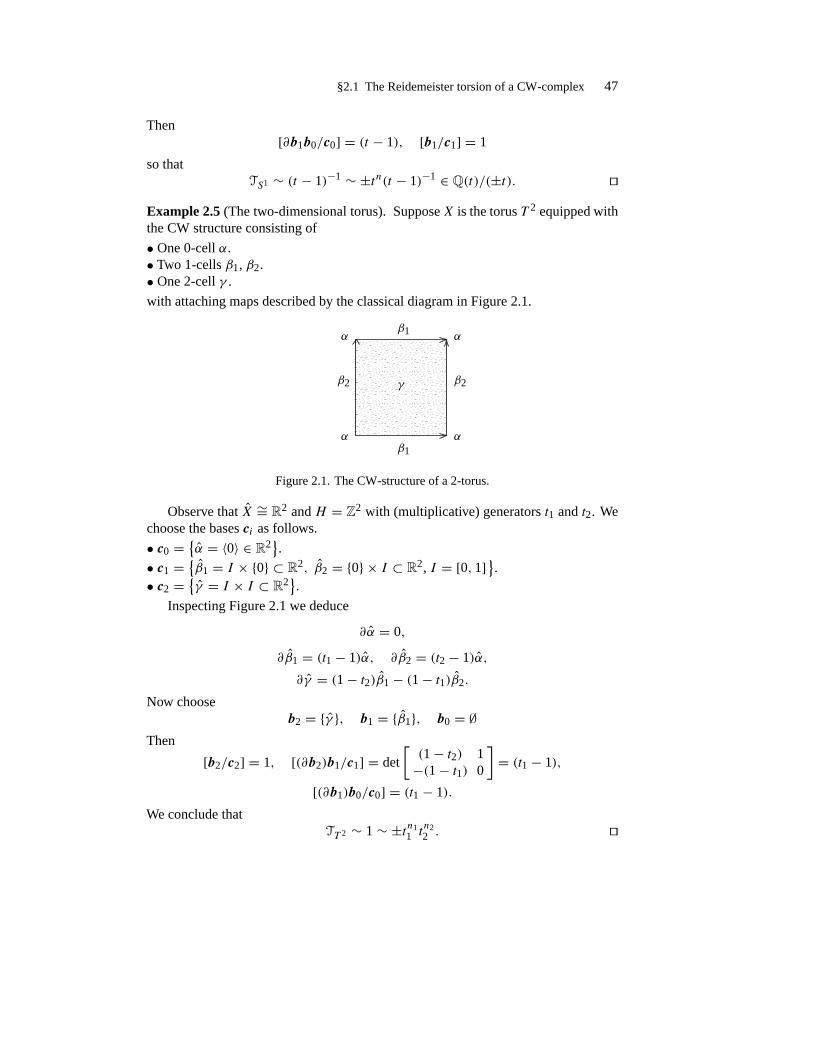
§2.1 The Reidemeister torsion of a CW-complex 47
Then[∂b1b0/c0] = (t − 1), [b1/c1] = 1
so thatTS1 ∼ (t − 1)−1 ∼ ±tn(t − 1)−1 ∈ Q(t)/(±t). �
Example 2.5(The two-dimensional torus). SupposeX is the torus T 2 equipped withthe CW structure consisting of
• One 0-cell α.• Two 1-cells β1, β2.• One 2-cell γ .
with attaching maps described by the classical diagram in Figure 2.1.
α
αα
α
β1
β1
β2β2 γ
Figure 2.1. The CW-structure of a 2-torus.
Observe that X ∼= R2 and H = Z2 with (multiplicative) generators t1 and t2. Wechoose the bases ci as follows.
• c0 ={α = 〈0〉 ∈ R2
}.
• c1 ={β1 = I × {0} ⊂ R2, β2 = {0} × I ⊂ R2, I = [0, 1]}.
• c2 ={γ = I × I ⊂ R2
}.
Inspecting Figure 2.1 we deduce
∂α = 0,
∂β1 = (t1 − 1)α, ∂β2 = (t2 − 1)α,
∂γ = (1− t2)β1 − (1− t1)β2.
Now chooseb2 = {γ }, b1 = {β1}, b0 = ∅
Then
[b2/c2] = 1, [(∂b2)b1/c1] = det
[(1− t2) 1−(1− t1) 0
]= (t1 − 1),
[(∂b1)b0/c0] = (t1 − 1).
We conclude thatTT 2 ∼ 1 ∼ ±tn1
1 tn22 . �
48 2 The Reidemeister torsion
Example 2.6(The higher dimensional tori). Suppose X is the n-dimensional torusX := Rn/Zn. Denote by ti the generators of the (multiplicative) group H := Zn ∼=π1(X). They determine a basis (ei) of the (additive) group Zn. For each orderedmulti-index I = 1 ≤ i1 < · · · < ik ≤ n we set
eI := ei1 ∧ · · · ∧ eik ∈ �kZn.The universal Abelian cover is Rn→ Rn/Zn and
Ck(X) ∼= Z[H ] ⊗Z �kH.
The monomials {eI ; |I | = k} determine a Z[ti , t−1j ]-basis (eI ) of Ck(X) defined by
eI ={(x1, . . . , xn) ∈ [0, 1]n; xj = 0 ∀j �∈ I}.
We use the wedge product to introduce a Z2-graded Z[H ]-algebra structure on C(X).The boundary operator
∂ : C(X)→ C(X)
is then more than just a morphism of Z[H ]-modules. It is an odd derivation uniquelydetermined by the conditions
∂e∅ = 0, ∂ei := (ti − 1)e∅, i = 1, . . . , n.
Equivalently, it can be defined as the contraction with the formal vector field
T :=∑k
(tk − 1)ek.
Fix an element u ∈ H , and form the Koszul map
κu : Ck(X)→ Ck+1(X), ω → u ∧ ω.For simplicity we let u := e1. Observe that
∂(e1 ∧ •)+ e1 ∧ ∂• = (1− t1)•so that, if we define
η : C(X)→ C(X), ω → (t1 − 1)−1e1 ∧ ωthen ∂η+η∂ = 1. Hence η is a contraction of the complex C(X). As in §1.1 we formthe operators
D = ∂ + η.The torsion of C(X) is then
TX ∼ det(D : Ceven(X)→ Codd(X)
).

§2.1 The Reidemeister torsion of a CW-complex 49
Set Ln := Zn. We have produced a sequence of operators
Dn : �evenLn ⊗Z Z[Ln] → �oddLn ⊗Z Z[Ln]such that det(Dn) = τ(T n). If we write Ln+1 = Ln ⊕ Z · en+1 then we obtaindecomposition
�evenLn+1 = �evenLn⊕�oddLn∧en+1, �oddLn+1 = �oddLn⊕�evenLn∧en+1.
Using these splittings we obtain the following block decomposition for Dn+1
Dn+1 =[Dn ∗0 Dn
],
whereDn = ∂ + η : �oddLn ⊗ Z[Ln] → �evenLn ⊗ Z[Ln].
Since DnDn = 1 we deduce
det(Dn+1) = 0, ∀n ≥ 1.
ThusTT n ∼ 1, ∀n > 1. �
The above identity is a consequence the following more general principle.
Example 2.7(The torsion of S1 ×X, X-finite cell complex). Denote by π both thenatural morphism
H1(S1 ×X)→ H1(S
1),
and the induced map
Q(H1(S1 ×X))→ Q(t) ∼= Q(H1(S
1)).
ThenTπS1×X ∼ (t − 1)−χ(X) ∼ T
χ(X)
S1 .
Observe that TπS1×X can be computed using the coverR×X→ S1×X. The associated
cell complex has a Z[t]-module structure. More precisely
C(R×X) ∼= C(R)⊗Z C(X),
where C(R) is the chain complex of Z[t]-modules discussed in Example 2.4,
0 → Z[t] (t−1)·−→ Z[t] → 0.
ThenCk(R×X) = Z[t]e1 ⊗ Ck−1(X)⊕ Z[t]e0 ⊗ Ck(X),

50 2 The Reidemeister torsion
with basise1 ⊗ Sk−1(X) ∪ e0 ⊗ Sk(X).
The boundary operator ∂ : Ck(R × X) → Ck−1(R × X) acts according to the pre-scriptions
∂(e1 ⊗ σk−1) = (1− t)e0 ⊗ σk−1 − e1 ⊗ ∂σk, ∂(e0 ⊗ σk) = e0 ⊗ ∂σk−1.
Define the morphism of Z[t]-module
η : Ck−1(R×X)→ Ck(R×X),
e0 ⊗ σk−1 → 1
t − 1e1 ⊗ σk−1, e1 ⊗ σk−2 → 0.
Observe that η2 = 0 and ∂η + η∂ = 1, i.e. η is an algebraic contraction. Then
TπS1×X = det
(∂ + η : Ceven(R×X)→ Codd(R⊗X)
).
With respect to the bases
e0 ⊗ S0(X) ∪ e1 ⊗ S1(X) ∪ e0 ⊗ S2(X) ∪ · · ·of Ceven, and
e1 ⊗ S0(X) ∪ e0 ⊗ S1(X) ∪ e1 ⊗ S2(X) ∪ e0 ⊗ S3(X) ∪ · · ·of Codd, the operator ∂ + η has the description
n0 columns n1 columns n2 columns · · ·
n0 rows (t − 1)−1 −∂ 0 · · ·
n1 rows 0 (t − 1) ∂ · · ·
n2 rows 0 0 (t − 1)−1 · · ·...
......
...
where nk := #Sk(X). We deduce
TπS1×X = (t − 1)−
∑k(−1)knk = (t − 1)−χ(X) = T
χ(X)
S1 . �
Example 2.8(The torsion of a product). The computations in the above example gen-eralize as follows. Suppose X and Y are compact CW-complexes. Denote by π boththe natural map
H1(X × Y )→ H1(X),

§2.1 The Reidemeister torsion of a CW-complex 51
and the induced morphism
Q(H1(X × Y ))→ Q(H1(X)).
ThenTπX×Y = T
χ(Y )X . (2.1)
To prove this consider the Abelian cover of X × Y induced by π . It coincides withX× Y , where X is the universal Abelian cover of X. Denote by (C(X), ∂0) the chaincomplex of Z[H1(X)]-modules generated by the CW-decomposition of X. Thenthe chain complex of Z[H1(X)] modules corresponding to the CW-decomposition ofX × Y has the form(
C(X × Y ), ∂) ∼= (C(X), ∂0) ⊗Z
(C(Y ), ∂Y
),
where the hat ˆover the ⊗ signs signifies that we are taking a graded tensor product.Suppose for simplicity (C(X), ∂0) is acyclic and denote by η an algebraic contraction.Now define
η : Ck−1(X × Y )→ Ck(X × Y )by the equality
η(σ ⊗ δ) = (ησ ) ⊗ δ,for every cell σ of X and every cell δ of Y . This morphism is an algebraic contractionof the complex C(X × Y ). Now order the cells of Y
δ1, δ2, . . .
as in (1.3) such thatdim δi ≥ dim δi+1.
Using the decomposition
Ceven/odd(X × Y ) ∼=⊕i
Cνi (X)⊗ δi,
where νi + dim δi = even/odd, we deduce that the operator
∂ + η : Ceven(X × Y )→ Codd(X × Y )has lower triangular form, and the i-th diagonal element
Cνi (X)⊗ δi → Cνi−1(X)⊗ δihas the form (
∂0 + η)(−1)νi
.
Formula (2.1) is now obvious. We refer to [31, 34, 35] for more information about thetorsion of a fiber bundle. �

52 2 The Reidemeister torsion
Example 2.9(The torsion of lens spaces). The lens space L(p, q) is defined as thequotient
L(p, q) := S3/(1,q ,
where for (r, p) = (s, p) = 1 we denote by (r,s the action of cyclic group Zp on
S3 := {(z1, z2) ∈ C2; |z1|2 + |z2|2 = 1}
defined by the rule
ζ (r,s (z1, z2) = (ζ rz1, ζsz2), ∀ζp = 1.
The maximal Abelian cover of L(p, q) is the sphere S3. To compute the torsion ofthe lens space L(p, q) we first need to produce a Zp-equivariant CW-decompositionof S3. For j ∈ Zp define
E0j ={(ζ j , 0) ∈ S3},
E1j ={(eiθ , 0) ∈ S3; 2πj
p≤ θ ≤ 2π(j + 1)
p
},
E2j ={(z1, sζ
j ) ∈ S3; t ∈ [0, 1]} = {(z1, sζj ) ∈ C2; s ∈ R,
√|z1|2 + s2 = 1
},
E3j ={(z1, z2) ∈ S3; 2πj
p≤ arg z2 ≤ 2π(j + 1)
p
}.
Each Ekj is homeomorphic to a closed k-ball, and the collection{Ekj}
0≤k≤3,j∈Zp
forms a Zp-equivariant decomposition of S3. Set
ckj := Int(Ekj ).
We orient the cells inductively over k such that, taking into account the orientations,we have
∂c2j =
p−1∑i=0
c1i ,
and∂c1j = c0
j+1 − c0j , ∂c3
j = c2j+1 − c2
j .
Observe that
ζ · ckj = ckj+1, k = 0, 1 and ζ · ckj = ckj+q, k = 2, 3.
Hence
∂c20 =( p−1∑j=0
ζ j)c1
0,
§2.1 The Reidemeister torsion of a CW-complex 53
and∂c1j = (ζ − 1)c0
j , ∂c3j = (ζ r − 1)c2
j ,
where r · q = 1 mod pZ. Suppose K is a field and ϕ : Z[ζ ] = Z[Zp] → K is anontrivial ring morphism. Set t := ϕ(ζ ) and Cϕ∗ := C∗(S3)⊗ϕ K. Observe that
Cϕk = K · ck0, k = 0, . . . , 3.
This shows the chain complex Cϕ∗ is acyclic and an elementary computation yields
Tϕ
L(p,q) ∼ (1− t)−1(1− t r )−1.
Observe that if we choose a different generator s of H1(L(p, q)
)defined by sq = t
we haveTϕ
L(p,q) ∼ (1− sq)−1(1− s)−1. � The torsion of a CW-complex depends on the CW-structure. The following result
states this more precisely. For a proof and more details we refer to [16, Chap. IV] or[72, §7].
Theorem 2.10(Combinatorial invariance of torsion). The torsion TX,Y is invariantunder subdivision of the CW-pair (X, Y ).
It is known that any compact smooth manifold admits C1-triangulations, and anytwo have a common finer subdivision (see [72, §9] for more details). This shows thatwe can define the torsion of a smooth manifold using C1-triangulations and the resultwill be independent of triangulations. In other words the following true.
Theorem 2.11. The torsion of a compact smooth manifold is a diffeomorphism in-variant.
Remark 2.12. The absolute torsion TX of a simplicial complex X is known to bea topological invariant of the cellular complex X; see [13]. However, the relativetorsion TX,Y is not a topological invariant; see the beautiful paper [69] or Remark 2.62,page 105. �
From the exact homology sequence of a pair and the multiplicativity of the torsionwe deduce the following result.
Theorem 2.13. Suppose (X, Y ) is a CW-pair, K is a field and ϕ : Z[H1(X)] → K isa ring morphism. If j denotes the inclusion induced morphism
j : Q(H1(Y ))→ Q(H1(X))
and either TjY �= 0 or T
ϕ◦jX,Y �= 0. Then
TϕX ∼ T
ϕX,Y · T ϕ◦jY .

54 2 The Reidemeister torsion
If f : X→ Y is a cellular map then we can form its mapping cylinder
Mf := (X × [0, 1] ∪ Y )/{(x, 1) = f (x)}.Y is a strong deformation retract of Mf and in particular, H1(Mf ) ∼= H1(Y ). Wedefine the torsion of f by the equality1
Tf := TMf ,X ∈ Q(H1(Y )).
If f is a homotopy equivalence then H1(X) ∼= H1(Y ) so the torsion of f is also anelement of Q(H1(X)). In general, the torsion of a homotopy equivalence may notbe ∼ 1. However, we have the following fundamental result of J. H. C. Whitehead([16, 19, 72]).
Theorem 2.14. If f is a simple homotopy equivalence then
Tf ∼ 1.
We will not present a formal, geometric definition of the notion of simple homotopy.We only want to mention a typical example of such homotopy: the collapse of a simplexonto one of its faces (see Figure 2.2). In general, a simple homotopy is a compositionof such elementary collapses.
Figure 2.2. Elementary collapse.
For example, a 3-manifold with boundary equipped with a simplicial decomposi-tion is simple homotopy equivalent to a 2-dimensional simplicial complex.
Using Theorem 2.13 and 2.14 we deduce that if two cellular complexes X, Y aresimple homotopy equivalent then
TX ∼ TY .
1The torsion of the pair (Mf , Y ) is known to be trivial, ∼ 1, (see [72, §7]).

§2.1 The Reidemeister torsion of a CW-complex 55
Example 2.15(The solid torus). The inclusion S1 ↪→ D2 × S1, p → (0, p) is asimple homotopy equivalence so that the torsion of a solid torsion is identical to thetorsion of a circle
TD2×S1 ∼ (t − 1)−1. � Using the multiplicativity property of the torsion and the Mayer–Vietoris sequence
we deduce the following consequence.
Theorem 2.16(Gluing Formula). Suppose X1, X2 are subcomplexes of X such that
X = X1 ∪X2 and X1 ∩X2 = Y.Suppose K is a field and ϕ : Q[H1(X)] → K is a ring morphism. Let
j : Q(H1(Y ))→ Q(H1(X)), jk : Q(H1(Xr))→ Q(H1(X)), k = 1, 2
denote the inclusion induced morphisms. If Tϕ◦jY �= 0 then
TϕX · T ϕ◦jY ∼ T
ϕ◦j1X1
· T ϕ◦j2X2.
Example 2.17(The torsion of fibrations over a circle). We follow closely the presen-tation in [33]. Suppose
F X
S1
� �j
��π
is a smooth fiber bundle over S1, with compact, closed, connected, oriented fiber F .Fix a Riemann metric onX such that π is a Riemann submersion. π defines a gradientflow which covers the canonical rotational flow on S1 (with period 2π ). We denoteby h : X→ X the time 2π -map of this flow. It induces a map
µ = h|F : F = π−1(0)→ π−1(2π) = Fknown as the geometric monodromy of this fibration.
Fix a cellular structure on F and a cellular approximation µ′ of the monodromymap µ and form the mapping torus X′ of µ′. One can show (see [33, 49]) that thetorsion of X is equal to the torsion of X′ and we will compute the torsion of X′. Thegroup Z acts on C∗(π−1(F );Z) by
t (k, σ ) = (k + 1, σ ),
so that we have the isomorphism of Z[t, t−1]-modules
C∗(π−1(F );Z) ∼= C∗(F,Z)⊗ Z[t, t−1].

56 2 The Reidemeister torsion
The natural projection π : X′ → S1 defines an infinite cyclic cover
π : X′π → X′,
the pullback of exp : R → R/2π iZ = S1 via π . The space X′ has a natural CW-structure which lifts to a CW-structure on the cover X′π . The cellular chain complexC∗(X′π ;Z) has a structure of Z[t, t−1]-module given by the actions of the group ofdeck transformations of X′π and can be described as the algebraic mapping torus ofthe morphism of Z[t, t−1]-cellular complexes
µ′π = tµ′ : C∗(π−1(F );Z)→ C∗(π−1(F );Z),(k, σ ) → (k + 1, µ′(σ )) = t (k, µ′(σ ))
Using the identity (1.6) in Example 1.6 we conclude that
T(C∗(X′π ;Z)
) ∼ ζµ(t),where ζµ(t) is the s-zeta function of the induced morphism µ∗ on the Z2-gradedvector space H∗(F,R). The map π induces a morphism H := H1(X)→ Z and thusa morphism
π : Q(H)→ Q(t).
The last equality can now be formulated
T πX ∼ ζµ(t).We refer to [33] for a description of the whole torsion ofX. The final result is howevernot so explicit.
To understand how much information about the torsion of X is contained in theabove equality we need to understand H1(X,Z). This homology can be determinedfrom the Wang exact sequence, [121, Chap. VII], which is a consequence of the factthat the chain complexC∗(X;Z) is the algebraic mapping torus ofC∗(F )with respectto µ∗,
· · · → Hk(F )1−µ∗−→ Hk(F )
j∗→ Hk(X)∩F−→ Hk−1(F )
1−µ∗−→ · · · .We obtain a short (split) exact sequence
0 → coker(1− µ∗)→ H1(X)→ Z→ 0.
The linear map H1(X)→ Z has a simple geometric interpretation: it is given by theintegral of the angular form
ω := 1
2ππ∗(dθ)
along a cycle c ∈ H1(X). Note that if
det((1− µ∗) : H1(F )→ H1(F )
) �= 0,

§2.1 The Reidemeister torsion of a CW-complex 57
then H1(X) has rank 1. In this case we have
TaugX ∼ ζµ(t).
If F happens to be a Riemann surface of genus g then, using the computations in §A.2we deduce
TaugX ∼ det
(1− tH1(µ)
)(1− t)2 . �
Example 2.18(The torsion of connected sums). Suppose N1 and N2 are two closed,oriented, triangulated, smooth 3-manifolds such that
ri := rankH1(Ni) > 0, i = 1, 2.
We want to prove thatTN1#N2 = 0,
i.e.H∗(N1#N2;Kπ ) �= 0,
where K is an arbitrary field entering into the decomposition of Q(H1(N1#N2)
), π
denotes the natural projection
Q(H1(N1#N2)
)→ K,
and Kπ denotes the corresponding local system of coefficients. We will follow anapproach we learned from Frank Connolly. We refer to [110, §4.3] for a differentproof of a slightly weaker result. Set N := N1#N2,
Gi := H1(Ni), G := H1(N1#N2) ∼= G1 ⊕G1.
Let Mi denote Ni with a small open disk Di removed and πi : Ni → Ni denote theuniversal Abelian cover of Ni . Set
Mi := π−1i (Mi).
Finally denote by S the 2-sphere M1 ∩M2 ⊂ N . The universal Abelian cover N ofN is obtained as follows.
• Fix a lift Di of Di to Ni , i = 1, 2 we can identify ∂Mi ∼= Gi × S2 so that
∂(G1 × M2) ∼= (G1 ⊕G2)× S2 ∼= ∂(G2 × M1).
For (g1, g2) ∈ G1 ×G2 we denote by ∂gi Mi the component of ∂Mi labelled by gi .
• Glue G1 × M2 to G2 × M1 along the boundary using the identifications (see Fig-ure 2.3).
{g1} × ∂g2M2 ∼ {g2} × ∂g1M1.
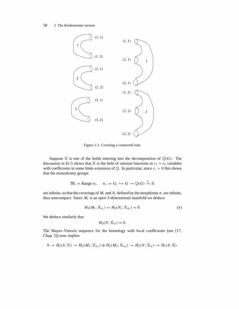
58 2 The Reidemeister torsion
(1, 1)(1, 1)
(1, 2)
(1, 2)(2, 1)
(2, 1)
(2, 2)
(2, 2)(3, 1)
(3, 1)
(3, 2)
(3, 2)
1
1
2
2
3
Figure 2.3. Covering a connected sum.
Suppose K is one of the fields entering into the decomposition of Q(G). Thediscussion in §1.5 shows that K is the field of rational functions in r1 + r2 variableswith coefficients in some finite extension of Q. In particular, since ri > 0 this showsthat the monodromy groups
Mi = Rangeπi, πi := Gi ↪→ G→ Q(G)π→ K
are infinite, so that the coverings ofMi andNi defined by the morphismsπi are infinite,thus noncompact. SinceMi is an open 3-dimensional manifold we deduce
H3(Mi;Kπi ) = H3(Ni;Kπi ) = 0. (∗)
We deduce similarly that
H3(N;Kπ ) = 0.
The Mayer–Vietoris sequence for the homology with local coefficients (see [17,Chap. 5]) now implies
0 → H2(S;K)→ H2(M1;Kπ1)⊕H2(M2;Kπ2)→ H2(N;Kπ )→ H1(S;K).
§2.2 Fitting ideals 59
Since S is simply connected we deduce that the last group is trivial and the first isisomorphic to K. We thus have a short exact sequence of K-vector spaces
0 → K→ H2(M1;Kπ1)⊕H2(M2;Kπ2)→ H2(N;Kπ )→ 0. (∗∗)
The middle part of (∗∗) can be determined from the long exact sequence of the pair(Ni,Mi):
0 → H3(Ni,Mi;K•)→ H2(Mi;Kπi )→ H2(Ni;Kπi )→ H2(Ni,Mi;K•)→ .
Using excision we deduce
0 → H3(Di, S;K)→H2(Mi;Kπi )→H2(Ni;Kπi )→H2(Di, S;K)→ 0. (∗∗∗)
The sequence (∗∗) implies
dimKH2(N;Kπ ) = dimKH2(M1;Kπ1)+ dimKH2(M2;Kπ2)− 1,
while (∗∗∗) impliesdimKH2(Mi;Kπi ) ≥ 1,
so that dimKH2(N;Kπ ) ≥ 1. �
§2.2 Fitting ideals
We interrupt for a little while the flow of topological arguments to discuss some basicalgebraic notions needed to go deeper inside the structure of torsion.
Let R be a Noetherian integral domain and denote by K its field of fractions.Suppose T : U → V is a morphism of free R-modules
U ∼= Rp, V ∼= Rq.Choosing bases in U and V we can represent T by a q × p matrix with entries in R,and we denote by I1(T ) ⊂ R the ideal generated by the entries of T . Clearly I1(T ) isindependent of the chosen bases of U and V . Equivalently, this means that I1(T ) isinvariant under elementary row and column operations on T . T induces morphisms
�kT : �kU → �kV,
and we setIk(T ) := I1(�kT ) ⊂ R.
In more concrete terms, Ik(T ) is the ideal generated by all the k × k minors of T .Observe that
R := I0(A) ⊃ I1(T ) ⊃ I2(T ) ⊃ · · ·

60 2 The Reidemeister torsion
and
Ik(T1 ⊕ T2) ⊃ Ik(T1)+ Ik(T2), Ik(T1 · T2) ⊂ Ik(T1) · Ik(T2), ∀k, T1, T2.
Suppose
UT→ V → M → 0
is a presentation of the finitely generated R-moduleM . Let g = rank V , r = rankU .Then g is the number of generators, while r is the number of relations of this presen-tation. Assume r ≥ g. Define
Fk(T ) := Ig−k(T ).Any other presentation can be obtained from the above by performing a succession ofelementary transformations described below, [92].
1. Change bases in U and V .
2. Replace U , V by R ⊕ U and R ⊕ V and T by 0 ⊕ T , where 0 denotes the trivialmap R→ R.
3. The reverse of 2.
4. Replace U by R ⊕ U T by T ◦ πU , where πU denotes the natural projectionR ⊕ U → U .
5. The reverse of 4.
Clearly the ideal Fk(T ) is invariant under these elementary transformations. Thisshows it is an invariant of the moduleM . It is called the k-th Fitting ideal, ofM andis denoted by Fk(M). Observe that
F0(M) ⊂ F1(M) ⊂ · · · ⊂ Fk(M) ⊂ · · · .F0(M) is called the order ideal of M and is denoted by O(M). In case M admits apresentation in which there are fewer relations than generators then we set O(M) =(0).
If R happens to be factorial then we define the order of M , ord(M) ∈ R/R×, asthe greatest common divisor of the elements in F0(M).
Example 2.19.
Fk(Rq) =
{0 if 0 ≤ k < qR if k ≥ q �
Example 2.20. SupposeG is the Abelian group generated by e1, e2, e3 subject to therelations
e1 + e2 + e3 = 0, 2e1 − e2 + 3e3 = 0, e1 = 3e3.
§2.2 Fitting ideals 61
Then it admits the presentation
Z3 A→ Z3 → G→ 0
where A is the 3× 3 matrix 1 2 11 −1 01 3 −3
.The order ideal is the ideal generated by | det(A)| = 13. It coincides with the orderof the group. In particular, ord(G) = ±13 ∈ Z/± 1. �
Example 2.21. Suppose M = R/I , I ⊂ R is an ideal of R. Then O(M) ∼= I .Indeed, if I is generated by n elements, thenM admits a presentation
RnL−→ R→ M → 0
so thatO(M) ∼= I1(L) = I. �
Example 2.22. SupposeM = Zn. Then
F0(M) = nZ, F1(M) = Z. � Proposition 2.23. SupposeM can be generated by q elements. Then(
annR(M))q ⊂ O(M) ⊂ annR(M) := {r ∈ R; r ·M = 0}.
Proof. Let x1, . . . , xq be generators ofM . If a1, . . . , rq ∈ annR(M) then we can forma presentation ofM containing the relations
aixj = 0, i, j = 1, . . . , q
which proves the first inclusion. To prove the second inclusion, consider a q × q-matrix of relations between the xi’s. Then, det(A)xi = 0, thus proving the secondinclusion. �
Corollary 2.24. Suppose R is a Noetherian integral domain. IfM is a submodule ofa free R module then O(M) ⊂ annR(M) = 0.
For a proof of the next result we refer to [55, XIX,§2].
Proposition 2.25.
Fn(M′ ⊕M ′′) =
∑r+s=n
Fr(M′)Fs(M ′′).
62 2 The Reidemeister torsion
Corollary 2.26.
Fk(M ⊕ Rq) = 0, ∀k < q, Fq(M ⊕ Rq) = O(M).
Example 2.27. Suppose R = Z and
M = Zn1 ⊕ · · · ⊕ Znk , nk|nk−1| · · · |n1.
Set N := n1 . . . nk . Then
F0(M) = NZ, F1(M) = N
n1Z, . . . , Fk−1(M) = N
n1 . . . nk−1Z, Fk(M) = Z. �
Example 2.28(The elementary invariants of a matrix). SupposeR = Z[t, t−1]. Anymatrix A ∈ SLn(Z) defines a R-module structure on Zn
p(t, t−1) · u := p(A,A−1)u, ∀p(t, t−1) ∈ R, u ∈ Zn.
We denote this is R-module by (Zn, A). It admits the presentation
Rnt−A−→ Rn
fA−→ (Zn, A)→ 0,
where fA is the map
Rn ∼= Zn ⊗Z R→ Zn,∑j
)uj tj → Aj )uj .
Denote by qi ∈ Z[t] the elementary invariants of A (see [55, XIV, §2]), i.e. the monicpolynomials uniquely determined by the conditions
qk|qk−1| · · · |q1, pA(t) := det(t − A) = q1 . . . qk,
such that, as aQ[t]-module, (Qn, A) is isomorphic to the direct sum of cyclic modules
(Qn, A) ∼=k⊕j=1
Q[t]/(qj ).
(Observe that qk is the minimal polynomial of A.) We deduce
F0(Zn, A) = ( pA(t) ), F1(Zn, A) =(pA(t)q1
), F2(Zn, A) =
(pA(t)q1q2
), . . . . �
§2.3 The Alexander function and the Reidemeister torsion 63
§2.3 The Alexander function and the Reidemeister torsion
Assume R is a Noetherian, unique factorization domain with 1 and
(C, ∂) : 0 → C�→ C�−1 → · · · → C1 → C0 → 0
is a chain complex of finitely generatedR-modules. We define the Alexander functionA(C) to be zero if ord
(Hi(C)
) = 0 for some i. Otherwise, we set
A(C) :=�∏j=0
ord(Hi(C)
)(−1)i+1.
Example 2.29(The circle revisited). The ring Z[t, t−1] is the localization of a fac-torial Noetherian ring and so itself must be factorial and Noetherian. Consider thecomplex of Z[t, t−1]-modules discussed in Example 2.4,
C : 0 → C1 = Z[t, t−1] ∂→ C0 = Z[t, t−1] → 0,
where δ is the multiplication by (t − 1). Then
H1(C) ∼= Z[t, t−1], ord(H1(C)
) ∼ 1,
H0(C) ∼= Z[t, t−1]/(1− t),so that (see Example 2.21)
ord(H0(C)
) ∼ (t − 1).
Thus A(C) ∼ (t − 1)−1. �
Example 2.30. Suppose U is a torsion module over R = Z[t, t−1] which is free asa Z-module. We deduce that the rank of U over Z is finite, say r . The polynomial tdefines an automorphism
A ∈ AutZ(U) ∼= SL(U) ∼= SL(r,Z), u → t · u.Then, according to Example 2.28 we have
ordZ[t,t−1] U ∼ pA(t) := det(t − A). �
Suppose (X, Y ) is a compact CW-pair. Set H := H1(X), F = H/Tors(H),denote by X→ X the universal (maximal) Abelian cover of X, and by aug : H → F
the natural projection. We can form the complex of Z[F ]-modules
Caug(X, Y ) := C(S(X), S(Y ))⊗aug Z[F ]. (2.2)

64 2 The Reidemeister torsion
Z[F ] is Noetherian and factorial so the Alexander function of this complex is anelement in Q(F ), well defined up to multiplication by a unit in the ring Z[F ]. Wedenote this Alexander function by A(X, Y ) and we will refer to it as the Alexanderfunction of the pair (X, Y ). The next result, due to Turaev, generalizes the computationin Example 2.29.
Theorem 2.31([33, 73, 111]). If (X, Y ) is a compact CW-pair then
TaugX,Y ∼ A(X, Y ) ∈ Q(F ).
Remark 2.32. The above result is similar in spirit with the classical Euler–Poincarétheorem which states that the Euler characteristic of a simplicial complex is equal tothe Euler characteristic of its homology. In the above theorem, T aug is defined interms of a simplicial (CW) decomposition while the Alexander function is definedentirely in homological terms. �
Proof. We follow the approach in [111]. This theorem is a consequence of thefollowing abstract result.
Lemma 2.33. Suppose R is a Noetherian, factorial ring of characteristic zero, K isits field of fractions and
C : 0 → Cm→ Cm−1 → · · · → C1 → C0 → 0
is a chain complex of free R-modules, equipped with a basis c such that
rankK H∗(C) = 0, i.e. H∗(C) = TorsH∗(C).
Then
T(C, [c]) = ζm∏j=0
ord(Hj(C)
)(−1)j+1,
where ζ is a unit of R.
Proof. Denote by Ji the cokernel of ∂i+1 : Ci+1 → Ci , and byAi the matrix describing
∂i+1 : Ci+1 → Ci
with respect to the basis c. Set ni := dimK Ci ⊗K and ri := dimKAi ⊗K. We havean exact sequence
0 → Hi(C)→ Ji → Ci−1,
and since Ci−1 is free we deduce that TorsHi(C) = Tors(Ji). Hence,
O(Hi(C)
) = O(Tors(Ji)
) *⇒ ord(Hi(C)) = ord(Tors(Ji)
). (2.3)

§2.3 The Alexander function and the Reidemeister torsion 65
On the other hand, observe that if B2i is any nonsingular square submatrix of A2i oforder r2i , 0 ≤ i ≤ #(m− 1)/2$, then there exists an unique τ -chain
{(S0, D0), . . . , (Sm−1, Dm−1)}such that D2i = B2i . Thus
det D2i = det(B2i ) ∈ O(Tors(J2i )
). (2.4)
If we write T(C, c) as an irreducible fraction x/y, we deduce from Proposition 1.5that
x/y =∏i≥0
det D2i+1/ det D2i
Since the r2i × r2i sub-matrix B2i in the equality (2.4) is arbitrary, we deduce that thedenominator y of T divides all the generators of
∏i≥0 O
(Tors (J2i )
)because they are
all of the form∏i≥0 detB2i . Hence
T(C, c) ·∏i≥0
O(Tors(J2i )
) ⊂∏i≥0
O(Tors(J2i+1)
).
The opposite inclusion
T(C, c)−1 ·∏i≥0
O(Tors(J2i+1)
) ⊂∏i≥0
O(Tors(J2i )
)is proved in a similar fashion. By writing T(C) = x/y, x, y ∈ R we deduce
x ·∏i≥0
O(Tors(J2i )
) = y ·∏i≥0
O(Tors(J2i+1)
).
Replacing O→ ord, and using (2.3) we deduce
x ·∏i≥0
ord(H2i (C)
) ∼ y ·∏i≥0
ord(H2i+1(C)
),
so that
T(C) ∼m∏j=0
ord(Hj (C))(−1)j+1
,
where we recall that ∼ denotes the equality up to multiplication by a unit of R. �
Definition 2.34. Suppose X is a finite CW-complex of dimension ≤ 2 and denote byF the free part of H1(X), F := H1(X)/Tors(H1(X)). The Alexander polynomial ofX is by defined by the equality
�(X) ∼ ord(H1(Caug(X)
)) ∈ Z[F ]where Caug(X) is defined as in (2.2). �
66 2 The Reidemeister torsion
Theorem 2.35([110, 111]). Let X be a finite CW-complex with χ(X) = 0 havingthe simple homotopy type of a finite two-dimensional cell complex. Then
TX ∈ N1(H1(X))/±H1(X),
and
TaugX ∼
�(X) if b1(X) ≥ 2
�(X)(t−1) if b1(X) = 1,
where in the second line t denotes a generator of the free part of H1(X).
Proof. We can consider X to be a finite two-dimensional cell complex with a singlezero-cell. Denote by m the number of 2-cells which we label by
t1, . . . , tm.
Since χ(X) = 0 the number of 1-cells is m+ 1 and we label them by
�0, �1, . . . , �m.
SetH := H1(X) and denote the maximal Abelian cover by X→ X. The 1× (m+1)-matrix with entries in Z[H ] representing the boundary operator
∂ : C1(X)→ C0(X)
has the form [�0 − 1 �1 − 1 · · · �m − 1
],
where �i denotes the element of H determined by the cell �i .The boundary operator ∂ : C2(X) → C1(X) is represented by a (m + 1) × m,
matrix D. Now choose
b2 = {t1, . . . , tm}, b1 = {�0, . . . , �m} \ {�k}
where �k is such that �k �= 0 ∈ H . Then
�(X) · (�k − 1) ∼ detD(k),
where D(k) is the matrix obtained from D by deleting the row corresponding to thecell �k . Thus
(1− h)TX ∈ Z(H), ∀h ∈ H.Using Proposition 1.27 we deduce that TX ∈ N1(H). The second part follows imme-diately from Theorem 2.31. We leave the details to the reader. �

§2.4 The Reidemeister torsion of 3-manifolds 67
§2.4 The Reidemeister torsion of 3-manifolds
The smooth, oriented manifolds are very special topological spaces and this specialstructure is reflected in their Reidemeister torsion as well. We will discuss in somedetail the simplest nontrivial situation, that of 3-manifolds.
One important distinguishing characteristic of an oriented manifold is the Poincaréduality. J. Milnor has shown that this phenomenon has a Reidemeister torsion coun-terpart; see [70].
Consider a smooth, compact, oriented n-dimensional manifold M . (We do notexclude the possibility that ∂M �= ∅.) We assumeM is triangulated and we denote byC(M) the corresponding simplicial chain complex. Denote by C�(M, ∂M) the dualcellular chain complex [67, §5.3], and by 〈•, •〉 the natural Poincaré pairing
〈•, •〉 : C�n−k(M, ∂M)× Ck(M)→ Z, k = 0, . . . , n.
More precisely, if σ is a k-simplex ofM andD(σ) denotes is dual (n−k)-polyhedronthen
〈D(σ), η〉 ={
1 if σ = η0 if σ �= η.
Set H := H1(M), and denote as usual by M → M the universal Abelian cover. Thesimplicial decomposition of M induces a simplicial decomposition (σ ) on M . Thisproduces a dual cellular decomposition
(D(σ )
). This is equivariant in the sense that
D(h · σ ) = h ·D(σ ), ∀σ , h ∈ H.C(M) has a natural structure ofZ[H ]-module. Using the involution ε ofZ[H ] inducedby the automorphism h→ −h of the additive group H we obtain a conjugate Z[H ]-module Cε(M). The equivariance of σ → D(σ ) shows that the Poincaré pairingextends to a Z[H ]- bilinear pairing
〈•, •〉 : C�(M)× Cε(M)→ Z[H ].SetF := H/Tors (H). Q(F ) is the field of rational functions in the variables t1, . . . , tb(b := b1(M)), and is equipped with the involution ε defined by ti → t−1
i . We getcomplexes
Caug(M) := C(M)⊗Z[H ] Q(F ), C�aug(M) := C�(M, ∂M)⊗Z[H ] Q(F ),
and a Q(F )-bilinear ε-pairing
C�aug(M, ∂M)× Cεaug(M)→ Q(F ).
The Poincaré duality implies that the complex C� computes the homology of the pair(M, ∂M) (with various twisted coefficient systems) and the above pairing is perfect.Using the abstract duality result in Proposition 1.21 we deduce
ε(T
augM
) · (T augM,∂M
)(−1)dimM+1 ∼ 1. (2.5)

68 2 The Reidemeister torsion
In particular, ifM is a 3-manifold then
ε(T
augM
) ∼ TaugM,∂M. (2.6)
If moreover χ(M) = 0 (which means that either ∂M is empty or it is an union of tori)then we deduce from the short exact sequence of the pair (M, ∂M) that
TaugM ∼ T
augM,∂M,
because T∂M ∼ 1. Thus, if χ(M) = 0 we have
ε(T
augM
) ∼ TaugM . (2.7)
More generally, ifK is one of the fields in the decomposition ofQ(H) andπ : Q(H)→K denotes the natural projection, then the involution ε on Q[H ] descends to an invo-lution on K we deduce that if TπM ∈ K \ {0} then
ε(T πM) ∼ T πM,∂M.
In particular, if we (non-canonically) regard TM as a function TM : H → Q, then theabove duality statements can be rephrased as
TM(h) ∼ TM(h−1)
meaning there exist ε = ε(M, ∂M) = ±1 and h0 ∈ H such that
TM(h−1) = εTM(hh0), ∀h ∈ H. (2.8)
Example 2.36. The smooth 3-manifolds with boundary admit cell decompositionswhich are simple homotopic to 2-dimensional cell complexes and thus they are coveredby Theorem 2.35. Suppose M is the complement of a knot K ↪→ S3, M ∼= S3 \K.Then H1(M) ∼= Z and
TM ∼ TaugM ∼ �K(t)/(1− t),
where �K(t) is the Alexander polynomial of S3 \K. The duality (2.7) is equivalentto
�K(t) ∼ �K(t−1).
The polynomial�K(t) is usually referred to as the Alexander polynomial of the knotK .More generally, if K ↪→ S3 is a link with n ≥ 2 components, then the torsion of
its exterior is an element in the group algebra Z[Zn] called the Alexander polynomialof the link. We refer to Appendix §B.1 on methods of computing the Alexanderpolynomial of a knot or link in S3. �
Exercise 2.1.SupposeK ↪→ S3 is a split link, i.e. there exists an embeddedS2 ↪→ S3,disjoint from K, such that each component of S3 \S2 contains at least one componentof K. Prove that the Alexander polynomial of K is trivial. (Hint: Use the samestrategy as in Example 2.18.) �

§2.4 The Reidemeister torsion of 3-manifolds 69
The Reidemeister torsion of a closed 3-manifold has special arithmetic properties.The next result, due to V. Turaev, summarizes some of them. Later on in §3.6 we willdiscuss more refined versions of these arithmetic properties.
Theorem 2.37([110, 111, 114]). LetM be a smooth, closed, oriented, three-manifold.Then
TM ∈ N2(H1(M))/±H1(M)),
and
TaugM ∼
�(M) if b1(M) ≥ 2
�(M)
(t−1)2if b1(M) = 1
0 if b1(M) = 0.
The original proof of this theorem can be found in [110] and is based on a cleveruse of the gluing formula (see also [112]). For a more elementary approach, basedon the definition of torsion, we refer to [114]. Corollary 1.41 implies the followingresult.
Corollary 2.38. Suppose M is a 3-manifold, possibly with boundary, and let G :=H1(M). If b1(M) > 0 then the complex Fourier transform of the torsion of M isa holomorphic on G \ {1}. If b1(M) > 1 then the complex Fourier transform is aholomorphic function on G.
The following result generalizes the classical fact stating that the sum of the coef-ficients of the Alexander polynomial of a knot in S3 is ±1.
Theorem 2.39(Alexander formula). SupposeM is an oriented 3-manifold such thatb1(M) = 1, r := |TorsH1(M)|. Then |�M(1)| = r .
Proof. Set H := H1(M), F : H/Tors(H) ∼= Z. We will consider only the specialcase when ∂M �= ∅. (For example, M is the complement of a knot in a rationalhomology sphere.) For the general case we refer to [112].
In this case M is simple homotopy equivalent to a 2-dimensional CW-complexX with a single 0-cell. We can assume that the closure of a one-dimensional cell isa circle which describes a generator t of F . We denote this circle by Y . From themultiplicativity properties of the torsion we deduce
�M(t) = TaugX · (t − 1) = T
augX,Y .
The chain complex Caug(X, Y ) of Z[H ] modules is very simple. It has no cells indimensions other that 1, 2 and the torsion is given by the determinant of the boundarymap
∂ : Caug2 (X, Y )→ C
aug1 (X, Y ).

70 2 The Reidemeister torsion
Ifmdenotes the number of 2-cells of (X, Y ) then we can regard ∂ as am×mmatrix withentries inZ[t, t−1]. We will write ∂(t) to emphasize this. The matrix ∂(1) := ∂(t)|t=1is the boundary map
C2(X, Y )→ C1(X, Y ),
and|�M(1)| = | det ∂(1)| = |H1(X, Y )| = |TorsH1(M)|. �
Remark 2.40. The above argument can be significantly strengthened. More precisely,suppose M is a closed oriented 3-manifold without boundary such that b1(M) = 1which is equipped with a CW decomposition. Fix an orientation of H1(M,R) andchoose a generator t of the free part ofH1(M) compatible with the above orientation.Fix ordered bases ck of the cellular complex Ck(M), k = 0, . . . , 3. The Alexanderpolynomial of M depends on these bases and we will denote this dependence by�M(t; c).
The Poincaré duality on M induces a canonical orientation on H∗(M,R) so thatthe canonical Euler isomorphism
Eul : DetC∗(M)⊗ R→ DetH∗(M,R)
can be identified with an real number
ε(c) ∈ {±1}.
Then one can show (see [114, Thm. 4.2.3]) that
ε(c)�M(1; c) = |TorsH1(M,Z)|.
We will have more to say about his issue later on in §3.5. �
§2.5 Computing the torsion of 3-manifolds using surgerypresentations
One of the most efficient methods for computing the torsion of a 3-manifold is basedon the following surgery formula due V. Turaev.
Theorem 2.41(Surgery Formula, [111]). Suppose K = K1∪· · ·∪Kn is an orientedlink in the interior of a compact, oriented 3-manifold X such that χ(X) = 0. Denoteby UK a tubular neighborhood of K in X. Then the natural morphism
α : H1(X \ UK)→ H1(X)
§2.5 Computing the torsion of 3-manifolds using surgery presentations 71
is an epimorphism and
α�(TX\UK
) = TX ·n∏i=1
(1− [Ki]
), (2.9)
where α� : N(H1(X \ UK)
) → N(H1(X)
)is the morphism induced by α described
in §1.5.
This result is an application of the multiplicativity property of the homological ex-act sequence of the pair (X,X \ UK). For more details about surgery we refer toAppendix §B.2.
Exercise 2.2.Prove Theorem 2.41. �
In applications it is much more convenient to use the Fourier transform of this formula.Set G = H1(X \ UK) and H = H1(X). The morphism α induces an injection
α : H ↪→ G
while the element [Ki] ∈ H defines via the Fourier transform a function
[Ki] : H → C, [Ki](χ) = χ([Ki]), ∀χ ∈ H .The surgery formula can now be rewritten as
α∗(TX\UK
) = TX ·n∏i=1
(1− [Ki]
). (2.10)
The formulation (2.10) has one major advantage over the formulation in (2.9). Moreprecisely, the product in (2.10) is the pointwise product in the algebra of complexvalued functions on H and the zero divisors of are given by the functions which arezero at some point of H . On the other hand, the zero divisors of the group algebraC[H ] are much harder to detect. From (2.10) we deduce
TX(χ) =
α∗(TX\UK
(χ))
∏ni=1
(1−χ([Ki ])
) if∏ni=1(1− χ([Ki])) �= 0
? if∏ni=1
(1− χ([Ki])
) = 0.
(2.11)
We can sometime fill in the question mark above using the following simple observa-tion.
Lemma 2.42. Suppose b1(X) > 0 and the homology classes [K1], . . . , [Kn] haveinfinite orders in H1(X). Then (2.11) uniquely determines TX.

72 2 The Reidemeister torsion
Proof. Set H = Hom(H,C∗). The complex Fourier transform TX of TX is holomor-phic on H \ {1} if b1(X) = 1, and in fact holomorphic on H if b1(X) > 1. If thehomology classes [Ki] have infinite orders in H for all i = 1, . . . , n then the zero set
Z :={χ ∈ H \ {1};
n∏i=1
(1− χ−1([Ki])
) = 0}
is an analytic subvariety of H \ {1} of positive codimension. This implies that H \ Zis dense in H . The function TX is unambiguously defined on H \ Z by (2.11), andadmits an unique holomorphic extension to H \ {1}. �
In the remainder of this section we will describe through examples how the aboveresults work in concrete applications.
Example 2.43(Trivial circle bundles over Riemann surfaces). Suppose X = S1 �g , where�g is an oriented Riemann surface of genus g. We will consider separatelythree cases.
1. g = 0, X = S1 × S2. Then X is obtained by gluing two solid tori along theirboundaries via the tautological identification. This shows that H1(X) = Z and usingthe surgery formula we deduce
TX = (1− t)−2.
2. g = 1, X = T 3. In this case we have
TX ∼ 1.
3. g ≥ 2. For simplicity we consider only the case g = 2. The manifold S1 ×� canbe obtained from two copies of S1 × T 2 using the fiber connect sum operation. Moreprecisely, consider two copies Y1, Y2 of the complement of a tiny open disk D ⊂ T 2
and setXi := S1 × Yi.
ThenT 3 = D × S1 ∪Xi,
and the inclusion induced morphism α : H1(Xi)→ H1(T3) is an isomorphism. From
the surgery formula (2.10) we deduce that
TXi ∼ TT 3 · (1− t) ∼ (1− t),where t denotes the homology class carried by the fiber. We have the decomposition
X := S1 ×�2 = X1 ∪X2, X0 := X1 ∩X2 ∼= T 2.

§2.5 Computing the torsion of 3-manifolds using surgery presentations 73
Denote by j k : H1(Xk) → H1(X), k = 0, 1, 2, the inclusion induced morphisms.The Mayer–Vietoris gluing formula implies
Tj 0X · TX0 ∼ T
j 1X1· Tj 2X2= (1− t)2. (2.12)
This shows j0 �= 0. We conclude that j0TX0 = 1 and
TX = (1− t)2.For Riemann surfaces of genus g we have
TS1×�g ∼ (ϕ − 1)2g−2.
This is in perfect agreement with the computations in Example 2.7. �
Example 2.44(Nontrivial circle bundles over Riemann surfaces). Consider a degree� circle bundle
S1 ↪→ N�→ �
over a Riemann surface of genus g ≥ 0. N� can be obtained form N0 using thefollowing procedure.
• Remove a tubular neighborhood U of a fiber of N0 so that U ∼= S1 ×D2 and set
V := N0 \ U ∼= S1 × (� \D2).
• Orient ∂U using the obvious diffeomorphism
∂U ∼= ∂D2 × S1.
Observe that the above diffeomorphism produces a canonical basis of H1(∂U) andhence an identification with Z2. Similarly, orient ∂V using the obvious diffeomor-phism
∂V ∼= ∂(� \D2)× S1.
This diffeomorphism produces a natural basis of H1(∂V ) and thus an identificationwith Z2. As in the previous example we deduce
TV ∼ (ϕ − 1)2g−3
where ϕ denotes the homology class carried by the fiber.
• Glue back U to V using the attaching map
�� :=[−1 0−� 1
].
To obtain more explicit results we need to rely on the Mayer–Vietoris sequence.

74 2 The Reidemeister torsion
Denote by α the natural morphism α : H1(V )→ H1(N�), and set G = H1(N�).Denote by β the natural morphism H1(U) → H1(N�). First, notice that H2(N�) istorsion free, of rank 2g and H2(V ) is torsion free of rank 2g, so that we can split thefollowing short exact portion off the Mayer–Vietoris sequence
0 → H1(T2)
jU⊕jV−→H1(U)
⊕H1(V )
β−α−→ H1(N�)→ 0.
Denote by c1, c2 the natural generators of T 2, and by ϕ, x1, . . . , x2g the natural gener-ators of H1(V ) (so that ϕ corresponds to the fiber and the xi’s generate H1(� \D2)).Also, denote by y the natural generator of H1(U). Finally, denote by IU and respec-tively IV the morphisms
IU : H1(∂U)→ H1(U), IV : H1(∂V )→ H1(V ).
In terms of the above generators we have
IV (c1) = 0, IV (c2) = ϕ, IU (c1) = 0, IU (c2) = y.Then jU = IU ◦ �−1
� , jV = IV , so that
jV : c1 → 0, c2 → y.
Since �−1� = �� we deduce
jU : c1 → −c1 − �c2 → −�ϕ, c2 → c2 → ϕ.
Using the bases {c1, c2} in H1(T2) and {y;ϕ, x1, . . . , x2g} in H1(U) ⊕ H1(V ) we
deduce that jU ⊕ jV has the (2g + 2)× 2-matrix description
A :=
0 1−� 10 0......
0 0
. (2.13)
Denote by � the sublattice of Z2g+2 generated by �ϕ, y + ϕ. Since ker(β − α) = �we deduce
α(ϕ�) = 0 and k := β(y) = α(ϕ)−1.
Re-label ϕ := α(ϕ). ϕ generates the torsion part ofH1(N�)which is a cyclic subgroupof order |�|. Moreover, k = ϕ−1 and using (2.11) we deduce
TN�(χ) ∼(χ(ϕ)− 1
)2g−2 if χ(ϕ) �= 1
? if χ(ϕ) = 1.

§2.5 Computing the torsion of 3-manifolds using surgery presentations 75
Observe that Lemma 2.42 is unapplicable in this case since ϕ is a torsion class. Wheng = 0, then N� can be identified with the lens space L(1,−�), and the only characterχ such that χ(ϕ) = 1 is the trivial character. In this case H1(N�) is a torsion group,and we have (see Theorem 2.37 of §2.4)
TN�(1) = 0.
To complete the determination of TN� for g > 0 we will rely on a twisted version ofthe Gysin sequence.
Consider a nontrivial character χ : H1(N�)→ S1 such that χ(ϕ) = 1. The usualGysin sequence of the fibrationN�→ � implies that χ factors through the morphismπ∗ : H1(N�)→ H1(�), i.e. there exists a nontrivial character χ : H1(�)→ S1 suchthat the diagram below is commutative:
H1(N�)
H1(�) S1.
�π∗
�����χ
�χ
The induced map χ : Z[H1(N�)] → C defines a system of local coefficients on N�which we denote by Cχ . Since χ factors through the morphism π∗ we deduce thatit defines a system of local coefficients on the total space X of the associated diskbundle. We denote this induced local system by Cχ . Using the Poincaré duality wededuce that we have isomorphisms
Hk(X,N�;Cχ ) ∼= H 4−k(X,Cχ ) ∼= H 4−k(�,Cχ ) ∼= Hk−2(�,Cχ ).
The homological long exact sequence of the pair (X, N�) can now be rewritten
· · · → Hk(N�,Cχ )→ Hk(�,Cχ )→ Hk−2(�,Cχ )→ · · · . (2.14)
Set bk(χ) := dimCHk(�,Cχ ) and e(χ) = b0(χ) − b1(χ) + b2(χ). Then e(χ) isindependent of χ and we have
e(χ) = e(1) = 2− 2g, ∀χ.On the other hand, when χ �= 1 then b0(χ) = b2(χ) = 0. This can be seen as follows.The 0-th cohomology space is naturally identified with the space global sections ofthe locally constant sheaf Cχ . Since χ is nontrivial there are no such sections. Hence
b0(χ) = 0, ∀χ �= 1.
On the other hand we have a Hodge–DeRham duality
∧: H 2(�,Cχ )×H 0(�,Cχ−1)→ H 2(�,C)
76 2 The Reidemeister torsion
so thatb2(χ) = b0(χ
−1) = 0, ∀χ �= 1.
Thus b0(χ) = b2(χ) = 0, ∀χ �= 1 and since e(χ) = 2− 2g we deduce
b1(χ) = 2− 2g, ∀χ �= 1.
Using this information in the fragment k = 1 of the sequence (2.14) we deduce thatwe have a surjection
H1(N�,Cχ )� H1(�,Cχ ).
In particular, if g > 1 we deduce H1(N�,Kχ ) �= 0 so that in this case
TN�(χ) = 0, ∀χ �= 1, χ(ϕ) = 1.
When g = 1 then H∗(N�,Cχ ) = 0 and from the sequence (2.14) we deduce
TN�(χ) ∼ 1.
Later in Example 2.57 we will explain how to extend the above technique to the moregeneral case of Seifert manifolds. For a different approach we refer to [31, 35]. Wealso want to refer to [34, §1,2] where it is explained how to obtain information aboutthe torsion of the total space of an arbitrary fiber bundle. �
It is known (see [41, 92, 96]) that any 3-manifold can be obtained from S3 by anintegral Dehn surgery on an oriented link in S3. A description of a 3-manifolds as aDehn surgery on a link is known as a surgery presentation of a 3-manifold and it is avery convenient way of operating with 3-manifolds. Many topological invariants canbe algorithmically read off a surgery presentation. We will spend the remainder of thissection explaining how to obtain almost complete information about the Reidemeistertorsion using surgery presentations. For the very basics concerning Dehn surgery werefer to Appendix §B.2 which we follow closely as far as the terminology and theorientation conventions are concerned. For a more in depth look at this importanttopological operation we refer to [41, 92, 96].
Suppose K = K1∪ · · ·∪Kn is an n-component oriented link in S3. We denote byE the complement of a tubular neighborhood U of K ↪→ S3. Then E is an oriented3-manifold with boundary. Moreover, H1(E) is a free Abelian group of rank n, andthe collection of oriented meridians
{µi; i = 1, . . . , n}defines an integral basis. We denote by λi the canonical longitude of Ki ↪→ S3
oriented such thatλi · µi = 1,
§2.5 Computing the torsion of 3-manifolds using surgery presentations 77
where the above intersection pairing is defined using the canonical orientation of ∂Eas boundary of E. H1(∂E) is a free Abelian group of rank 2n and the collection
{λi, µj ; i, j = 1, . . . n}is an integral basis. Set
�ij = Lk(Ki ,Kj ) = Lk(Kj ,Ki ),
where Lk denotes the Z-valued linking number of two disjoint knots in S3. Then theinclusion induced morphism
j : H1(∂E)→ H1(E)
is described in the above bases by
µj → µj , λi →∑k �=i�kjµk.
We perform an integral Dehn surgery on this link with coefficients )d = (d1, . . . , dn) ∈Zn. The attaching curves of this surgery are
ci = diµi + λi, i = 1, . . . n.
Denote resulting manifold byM )d . The natural morphism
α : H1(E)→ H1(M )d ,Z)
is onto, and leads to the following presentation of H1(N,Z)
H1(∂E) ⊃ spanZ{ci; i = 1, . . . , n} j−→ H1(E)� H1(M )d)→ 0,
ci → diµi +∑k �=i�kiµk.
We denote by P = P )d the symmetric n× n matrix with entries
pij ={�ij if i �= jdi if i = j.
The above presentation can be rewritten in the computationally friendly from
ZnP )d−→ Zn � H1(M )d)→ 0. (2.15)
The cores of the attaching solid tori define homology classes inM )d which for simplicitywe denote by ki . Algebraically, these homology classes are the images via α of

78 2 The Reidemeister torsion
Ki ∈ H1(E), i = 1, . . . , n, where Ki = jλ′i , and λ′i ∈ H1(E) are homology classesdetermined by the conditions
λ′j · ci = δij , i, j = 1, . . . , n.
For example, we can pickλ′j = −µj .
To compute the torsion ofM )d we use the following consequence of Turaev’s surgeryformula Theorem 2.41.
Corollary 2.45.
α�(TE) ∼ TM )d ·
n∏i=1
(1− ki ), (2.16)
where α� : N(H1(E)
) → N(H1(M )d)
)is the morphism induced by α described in
§1.5.
As explained before, it is convenient to use the Fourier transform trick describedin §1.6. To ease the presentation we set
G := H1(E), H = H1(M )d).
Then α : G→ H is an epimorphism, and by passing to duals we get an injection
α : H ↪→ G.
We can thus view H as a subgroup of G. The Fourier transform of TE is a (generalized)function TE on G, and the Fourier transform of TM )d is a (generalized) function TM )don H . Then (2.16) becomes the linear equation
TE(χ) = TM )d (χ) ·n∏i=1
(1− χ(Ki)
), ∀χ ∈ H ↪→ G. (2.17)
The homology classes ki ∈ H are represented by the vectors
Ki = −µi ∈ G ∼= Zn.For each χ ∈ H we set χi := χ([µi]), where [µi] := α(µi) ∈ H . We can nowrewrite (2.16) as
TE(χ1, . . . , χn) = TM )d (χ1, . . . , χn) ·n∏i=1
(1− χi
). (2.18)
The next example will illustrate the strengths and limitations of the above surgeryformula.
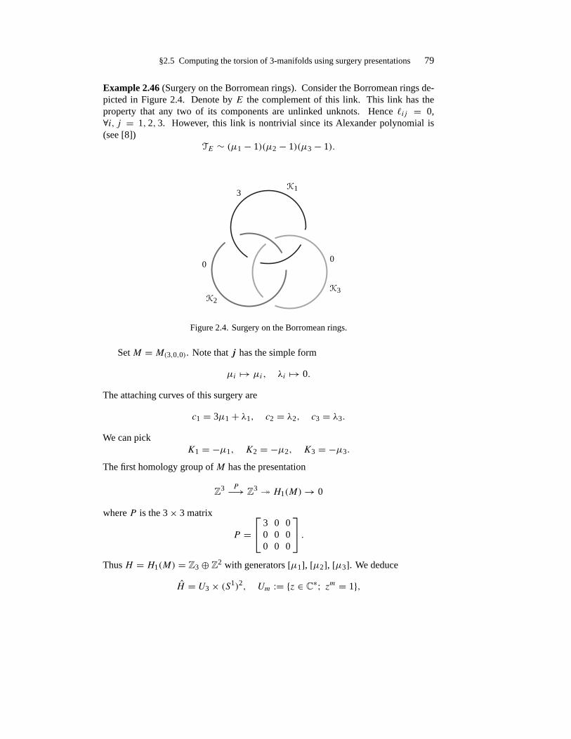
§2.5 Computing the torsion of 3-manifolds using surgery presentations 79
Example 2.46(Surgery on the Borromean rings). Consider the Borromean rings de-picted in Figure 2.4. Denote by E the complement of this link. This link has theproperty that any two of its components are unlinked unknots. Hence �ij = 0,∀i, j = 1, 2, 3. However, this link is nontrivial since its Alexander polynomial is(see [8])
TE ∼ (µ1 − 1)(µ2 − 1)(µ3 − 1).
3
00
K1
K2
K3
Figure 2.4. Surgery on the Borromean rings.
SetM = M(3,0,0). Note that j has the simple form
µi → µi, λi → 0.
The attaching curves of this surgery are
c1 = 3µ1 + λ1, c2 = λ2, c3 = λ3.
We can pickK1 = −µ1, K2 = −µ2, K3 = −µ3.
The first homology group ofM has the presentation
Z3 P−→ Z3 � H1(M)→ 0
where P is the 3× 3 matrix
P = 3 0 0
0 0 00 0 0
.Thus H = H1(M) = Z3 ⊕ Z2 with generators [µ1], [µ2], [µ3]. We deduce
H = U3 × (S1)2, Um := {z ∈ C∗; zm = 1},

80 2 The Reidemeister torsion
and (2.18) becomes
(χ1 − 1)(χ2 − 1)(χ3 − 1) ∼ TM(χ1, χ2, χ3)(1− χ1)(1− χ2)(1− χ3),
∀χ1, χ2, χ3 ∈ S1, χ31 = 1. We deduce
TM(χ1, χ2, χ3) ∼ 1, ∀χ1 �= 1, χ2 �= 1, χ3 �= 1.
Fix χ1 �= 1. Then TM(χ1, χ2, χ3) is a Laurent polynomial in χ2, χ3 so that we deduce
TM(χ1, χ2, χ3) ∼ 1, ∀χ1, χ2, χ3, χ1 �= 1.
We notice that the surgery formula contains no information about TM(1, χ2, χ3). Thisis the Fourier transform of T
augM , which according to Theorem 2.37 is the Alexander
polynomial ofM . �
Motivated by Lemma 2.42 we isolate a special class of surgeries.
Definition 2.47. A closed 3-manifold M satisfying b1(M) > 0 is said to admit anondegenerate surgery presentation if there exists an oriented link K = K1 ∪ · · · ∪Kn ⊂ S3, and surgery coefficients )d ∈ Zn such that ifM ∼= M )d , and all the homologyclasses kj have infinite orders in H1(M )d). �
The nondegenerate surgeries can be easily recognized using the following elemen-tary algebraic result.
Proposition 2.48. Consider an n-component oriented link K ↪→ S3, and a vector)d ∈ Zn. Set G := H1(S
3 \ K). The surgery defined by the coefficients )d is non-degenerate if and only if for every i = 1, . . . , n there exists )wi ∈ Hom(G,Z) suchthat
〈 )wi, P )dµj 〉 = 0, ∀j = 1, . . . , n, and 〈 )wi, µi〉 �= 0.
Exercise 2.3.Prove Proposition 2.48. �
The proof of the following result is a simple exercise in Kirby calculus ([115,§3.8]).
Proposition 2.49. Any 3-manifoldM withb1(M) > 0 admits a nondegenerate surgerypresentation.
Example 2.50. To fix the “deficiency” of the surgery described in Example 2.46 weslide K2 over K1. The link and the surgery coefficients change as indicated in Fig-ure 2.5. This surgery is nondegenerate and produces the same 3-manifold as thesurgery in Example 2.46. The new problem we are facing is the computation of theAlexander polynomial of the new link. We leave the quite unpleasant computation tothe reader.
�
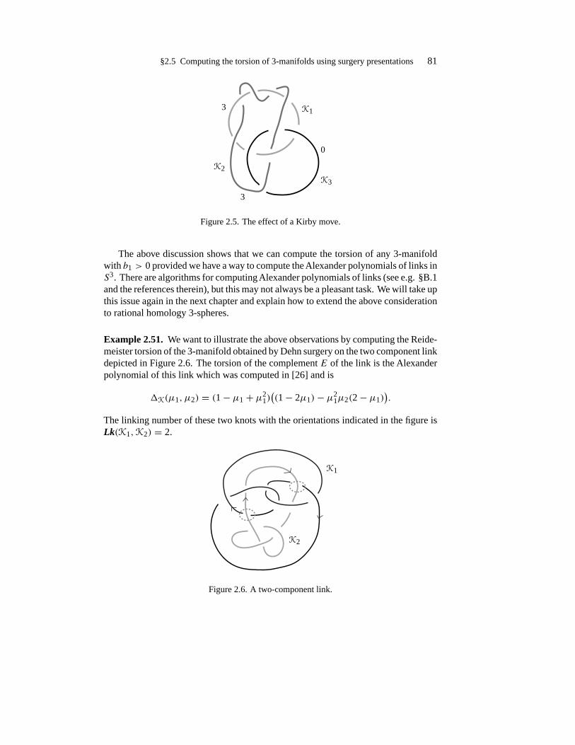
§2.5 Computing the torsion of 3-manifolds using surgery presentations 81
3
3
0
K1
K2
K3
Figure 2.5. The effect of a Kirby move.
The above discussion shows that we can compute the torsion of any 3-manifoldwith b1 > 0 provided we have a way to compute the Alexander polynomials of links inS3. There are algorithms for computing Alexander polynomials of links (see e.g. §B.1and the references therein), but this may not always be a pleasant task. We will take upthis issue again in the next chapter and explain how to extend the above considerationto rational homology 3-spheres.
Example 2.51. We want to illustrate the above observations by computing the Reide-meister torsion of the 3-manifold obtained by Dehn surgery on the two component linkdepicted in Figure 2.6. The torsion of the complement E of the link is the Alexanderpolynomial of this link which was computed in [26] and is
�K(µ1, µ2) = (1− µ1 + µ21)((1− 2µ1)− µ2
1µ2(2− µ1)).
The linking number of these two knots with the orientations indicated in the figure isLk(K1,K2) = 2.
K1
K2
Figure 2.6. A two-component link.

82 2 The Reidemeister torsion
We perform a (4, 1) surgery on this link, and we denote by M the resulting3-manifold. The group H = H1(M) admits the presentation
F1 = spanZ(c1, c2)P−→ F0 = spanZ(µ1, µ2)→H → 0,
where
P =[
4 22 1
]Also,
K1 = −µ ∈ F1, K2 = −µ2 ∈ F1.
Using the MAPLE procedure ismith we obtain[1 00 0
]= UPV, U =
[0 11 −2
], V =
[0 −11 2
]This means that the bases {V c1, V c2} in F0 and {U−1µ1, U
−1µ2} diagonalize thepresentation matrix P . The coordinates of µ1 and µ2 in the new basis are
µ1 →[
01
], µ2 →
[12
].
We denote by g the generator in H . We deduce that
k1 = −g, k2 = 2g,
so that both these homology classes have infinite orders. In other words, this surgeryis nondegenerate. Let χ ∈ H \ {1}. The surgery formula (2.17) becomes
(1− χ + χ2) · ((1− 2χ)− χ2χ−2(2− χ)) ∼ TM(χ) · (1− χ−1)(1− χ2)
so that(1− χ + χ2)(1+ χ) ∼ TM(χ)(1− χ)2(1+ χ)
which implies
TM(χ) ∼ 1− χ + χ2
(1− χ)2 .
�
Exercise 2.4.Compute the torsion of the 3-manifold obtained from the Dehn surgerydepicted in Figure 2.5. �

§2.6 Plumbings 83
§2.6 Plumbings
In this section we want to describe a special yet large class of 3-manifolds, and thenoutline a method for computing their torsions. These 3-manifolds, known as graphmanifolds, or plumbings, play an important role in the study of isolated singularitiesof complex surfaces. They are all obtained by gluing elementary pieces of the formS1�, where� is a surface with boundary. We begin by describing a combinatorialmethod of cataloging these manifolds.
Start with a graphG. We denote by V the set of vertices and byE the set of edges.The edges are oriented. We do not exclude the possibility that the graph has tails2.We denote by T the set of tails, so that T ∩ E = ∅. Multiple edges connecting thesame pair of vertices or loops are also allowed. For each edge e we denote by v±(e)the final/initial point. For each vertex we denote by E±v the set of outgoing/incomingedges, and by Tv the set of tails at v. Set Ev = E+v ∪ E−v , deg± v = |E±v |, tv = |Tv|,and deg v = deg+ v + deg− v + tv .
A decoration of G is a function
� : E→ SL2(Z), e → �(e).
A weight on G is a function g : V → Z≥0. Denote by C the 2× 2 matrix
C =[−1 0
0 1
].
Suppose (G, V,E, T , g, �) is a weighted decorated graph. We construct a 3-manifoldwith boundary as follows.
• Associate to each v ∈ V a Riemann surface �v with deg v boundary components.Fix a bijection between the components of ∂�v and Ev ∪ Tv . Set Mv := S1 × �v ,and denote by v the fiber of this trivial fibration over �v .
• For each v ∈ V and each e ∈ Ev fix an orientation preserving diffeomorphismbetween the component ∂eMv ofMv and the oriented standard torus v × ∂e�v .• For each edge e ∈ E glue the torus ∂eMv−(e) to the torus ∂eMv+(e) using theorientation reversing diffeomorphism which is described by the matrix C ◦�(e) withrespect to the oriented bases([∂e�v−(e)], [ v−(e)]), ([∂e�v+(e)], [ v+(e)])of H1(∂eMv±(e)).
After the above identifications we obtain an oriented 3-manifold with |T | boundarycomponents. We denote it byM(G) and we will say thatM is a generalized plumbingdescribed by the weighted decorated graphG. G is also known as the plumbing graph.
2A tail is an arc with one boundary component a vertex of the graph, while the other is free.

84 2 The Reidemeister torsion
This is related to the traditional plumbing construction described in [46, §8] wherethe decorations have the special form
�(e) = ±Pm,n := ±[
m 1mn− 1 n
]= ±Tn�Tm,
where
� =[
0 1−1 0
], Tk =
[1 0k 1
], ∀k ∈ Z.
To see this, note that
CPm,n =[ −1 0−n 1
].
[0 11 0
] [ −1 0−m 1
],
and the expression in the right hand side is exactly the description of the attachingmap in [46, p.67]. Observe also that �2 = −1 and Tm ◦ Tn = Tm+n, ∀m, n ∈ Z.
Despite its name, the generalized plumbing construction does not produce moremanifolds that the usual plumbing. To see this we will describe a few simple methodsof simplifying the combinatorics of a decorated graph G which do not affect thetopology ofM(G). Assume for simplicity that there are no tails.
If G(V,E, {Mv}, �) is a weighted, decorated graph we define its conjugate withrespect to a subset S ⊂ E to be the graph GS(V , ES, S, �S) such GS has the sameedges asG but the ones in S have opposite orientations while the others are unchanged.Moreover
�S(e) =�e if e ∈ E \ SC�−1
e C if e ∈ SObserve that CT −1
m C = Tm and CP−1m,nC = Pn,m.
Proposition 2.52. For any weighted decorated graphG(V,E, {Mv}, �) and any sub-set S ⊂ E the generalized plumbingsM(G) andM(GS) are diffeomorphic.
Exercise 2.5.Prove the above proposition. �
Figures 2.7 and 2.8 represent pairs of conjugate weighted decorated graphs de-scribing in one instance a circle bundle over a Riemann surface and in the secondinstance a simple plumbing.
00 TdTd gg=
Figure 2.7. A degree d circle bundle over a Riemann surface of genus g.
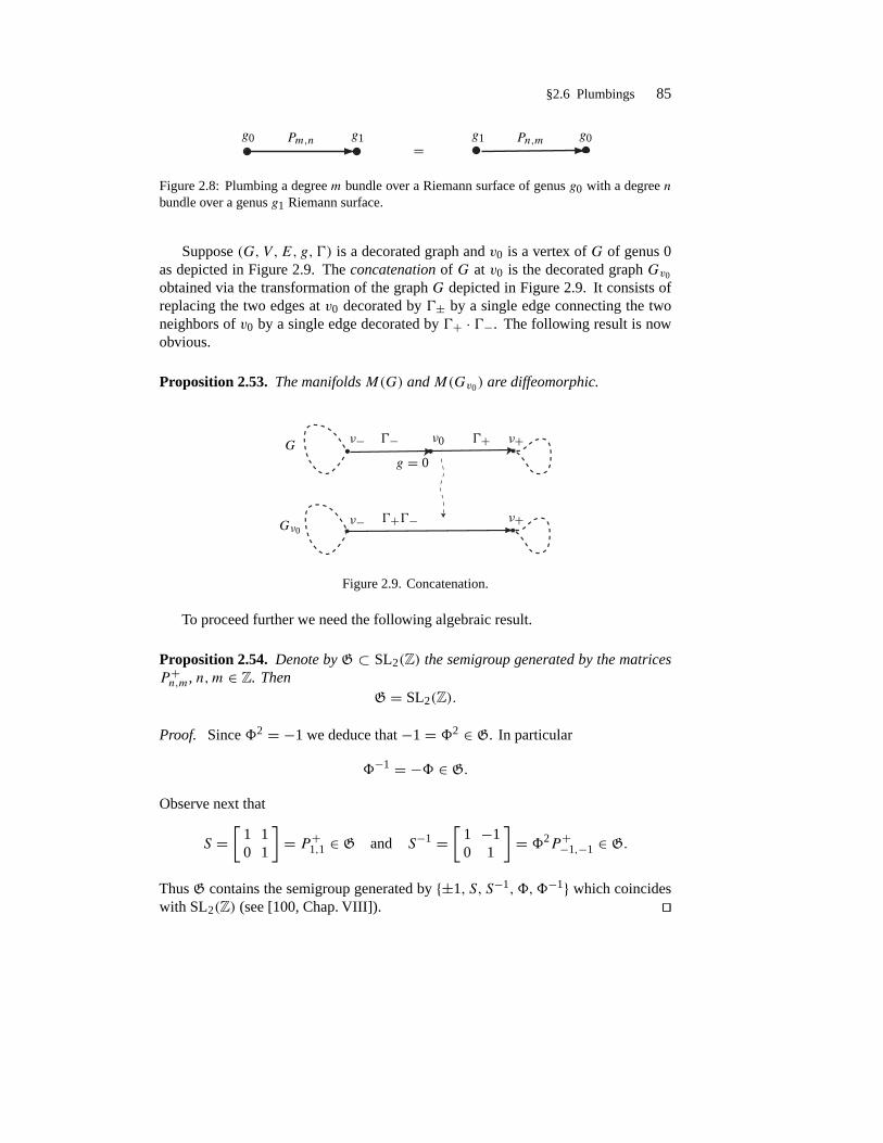
§2.6 Plumbings 85
g0g0 Pm,n g1g1=
Pn,m
Figure 2.8: Plumbing a degree m bundle over a Riemann surface of genus g0 with a degree nbundle over a genus g1 Riemann surface.
Suppose (G, V,E, g, �) is a decorated graph and v0 is a vertex of G of genus 0as depicted in Figure 2.9. The concatenation of G at v0 is the decorated graph Gv0
obtained via the transformation of the graph G depicted in Figure 2.9. It consists ofreplacing the two edges at v0 decorated by �± by a single edge connecting the twoneighbors of v0 by a single edge decorated by �+ · �−. The following result is nowobvious.
Proposition 2.53. The manifoldsM(G) andM(Gv0) are diffeomorphic.
G
ν−
ν− �− �+
ν+
ν+g = 0
Gν0�+�−
ν0
Figure 2.9. Concatenation.
To proceed further we need the following algebraic result.
Proposition 2.54. Denote by G ⊂ SL2(Z) the semigroup generated by the matricesP+n,m, n,m ∈ Z. Then
G = SL2(Z).
Proof. Since �2 = −1 we deduce that −1 = �2 ∈ G. In particular
�−1 = −� ∈ G.
Observe next that
S =[
1 10 1
]= P+1,1 ∈ G and S−1 =
[1 −10 1
]= �2P+−1,−1 ∈ G.
Thus G contains the semigroup generated by {±1, S, S−1,�,�−1} which coincideswith SL2(Z) (see [100, Chap. VIII]). �

86 2 The Reidemeister torsion
The above proposition implies that by applying the concatenation trick severaltimes we can transform any decorated graph into one in which all the decorations areof the formP±m,n. Thus any manifold which can be obtained by a generalized plumbingcan also by obtained by a traditional plumbing.
Figure 2.10. A sphere with several holes.
Any compact, oriented Riemann surface, possibly with boundary, can be decom-posed into Riemann surfaces of genus zero of the type depicted in Figure 2.10. Wehave thus proved the following result.
Corollary 2.55. Any generalized plumbing is diffeomorphic with a regular plumbingof circle bundles over Riemann surfaces of genus zero.
When the plumbing graph has no loops3 the combinatorics of the problem simpli-fies somewhat in the case of usual plumbings of circle bundles over spheres. First, weno longer have to keep track of the genera of the vertices, since g(v) = 0, for all v. Adecoration can now be identified with a pair of integers m±(e), and a sign ε(e) = ±1so that
�(e) = ε(e)Tm+�Tm−Due to the equality CP−1
m,nC = Pn,m we deduce from the conjugation trick that theorientation of the edge e is irrelevant. The decorated graph of a plumbing can besimplified by performing the changes indicated in Figure 2.11.
±Pm,n
m ± n
Figure 2.11. Describing a regular plumbing.
Define the Chern number of a vertex to be
c1(v) =∑e∈E−v
m−(e)+∑e∈E+v
m+(e).
3These correspond to selfplumbings and lead to quite subtle phenomena; see [37].

§2.6 Plumbings 87
The decorated graph then describe plumbings of circle bundles of degree c1(v) overspheres, according to the undecorated graph. In the left-hand-side Figure 2.12 we
00
00
++
++++
++
−1
−1
−1−1
−1
−1−1−1
−2
−2−2
−2
Figure 2.12. Plumbing −2-bundles over spheres.
have the decorated graph describing a plumbing of bundles over spheres. Each vertexhas Chern number −2. The usual graphical representation of this plumbing (definedin [46, §8]) is shown in the right-hand side of Figure 2.12. In general, we will drop thenumbersm±(e) attached to the edges of the graph, and we replace them with numbersc1(v) attached to the vertices. From now own, we will use only this description ofplumbings over spheres. We will refer to this plumbing description as the usual,regular, traditional etc. If additionally, all the edges have the same sign + we will nolonger indicated it on the plumbing graph.
An usual plumbing diagram can be transformed so that the resulting manifold doesnot change. For more details on this calculus with plumbings we refer to [78].
To compute the torsion of a plumbing we need to produce a surgery descriptionof such a 3-manifold. Fortunately there is a simple way to do this. We follow closelythe prescriptions in [37, 78]. Assume for simplicity that there are no loops4.
mm
m
nn
n+/−
(+) (−)
Figure 2.13. Surgery description of plumbings.
First, mark edges e1, . . . , em of the graphG so that the graph obtained by removing
4We can eliminate them by concatenation.
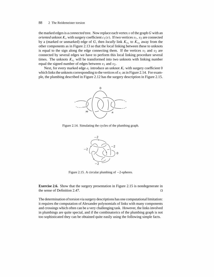
88 2 The Reidemeister torsion
the marked edges is a connected tree. Now replace each vertex v of the graphGwith anoriented unknotKv with surgery coefficient c1(v). If two vertices v1, v2 are connectedby a (marked or unmarked) edge of G, then locally link Kv1 to Kv2 away from theother components as in Figure 2.13 so that the local linking between these to unknotsis equal to the sign along the edge connecting them. If the vertices v1 and v2 areconnected by several edges we have to perform this local linking procedure severaltimes. The unknots Kvi will be transformed into two unknots with linking numberequal the signed number of edges between v1 and v2.
Next, for every marked edge ei introduce an unknot Ki with surgery coefficient 0which links the unknots corresponding to the vertices of ei as in Figure 2.14. For exam-ple, the plumbing described in Figure 2.12 has the surgery description in Figure 2.15.
0
m n
Figure 2.14. Simulating the cycles of the plumbing graph.
−2
−2
−2
−2
0
Figure 2.15. A circular plumbing of −2-spheres.
Exercise 2.6.Show that the surgery presentation in Figure 2.15 is nondegenerate inthe sense of Definition 2.47. �
The determination of torsion via surgery descriptions has one computational limitation:it requires the computation of Alexander polynomials of links with many componentsand crossings which often can be a very challenging task. However, the links involvedin plumbings are quite special, and if the combinatorics of the plumbing graph is nottoo sophisticated they can be obtained quite easily using the following simple facts.

§2.6 Plumbings 89
Proposition 2.56. (a) If the link K′ is obtained from the link K by adding an additionalcomponent C which is the meridian of a component Ki of K then
�K′ ∼ (µi − 1) ·�K. (2.19)
(b) (Seifert–Torres formula, [98, 109].) Denote by K′ the link is obtained from thelink K = K1 ∪ · · · ∪Kn by adding a component Kn+1 which is a simple closed curveon the boundary a thin tubular neighborhood of Kn of the form pλn + qµn, p �= 0.Then
�K′(µ1, . . . , µn+1) = �K(µ1, . . . , µpnµn+1)(T
pµn+1 − 1), (2.20)
where T =∏ni=1 µ�ii , �i = Lk(Ki ,Kn+1). Moreover, if K′′ denotes the link obtained
from K′ by removing the component Kn then
�K′′(µ1, . . . , µn−1, µn+1) = �K(µ1, . . . , µn−1, µpn ) · T
p − 1
T − 1. (2.21)
Exercise 2.7.Prove, without relying on (2.19), that the Alexander polynomial of thelink depicted in Figure 2.16 is∼ (1−µ), where µ denotes the meridian of the middlecomponent. (Hint: Find a simple CW-decomposition of the exterior of this link, oruse the Fox free calculus in §B.1.) �
Figure 2.16. A simple link.
Exercise 2.8.Prove the identity (2.19). (Hint: Fix a tubular neighborhood Ui of Kicontaining C. This allows us to regard the exterior of K as a subset of the exteriorof K′. Now use the Mayer–Vietoris theorem coupled with the computation in theprevious exercise.) �
Exercise 2.9.Prove (2.20) and (2.21). �
Exercise 2.10.Use (2.21) to compute the Alexander polynomial of the (3, 5)-torusknot depicted in Figure 2.17. �
If the graph G of a plumbing is a (connected) tree, all its edges are positive, andK = (Kv)v∈V is its associated link, then an iterated application of the trick (2.19)

90 2 The Reidemeister torsion
Figure 2.17. A MAPLE rendition of the (3, 5)-torus knot.
produces the equality
TS3\K ∼n∏i=1
(µv − 1)deg v−1. (2.22)
Things get much more complicated when the plumbing graph has cycles. In ournext examples we want to describe how to compute the torsion for simply connectedplumbing graphs and for the simplest non simply connected plumbing graphs.
Example 2.57(The torsion of Seifert manifolds. The case b1 > 0.). Consider thestar-shaped generalized plumbing graph depicted in Figure 2.18. The center of thestar has genus g. All the other vertices have genus zero. All Seifert manifolds can bedescribed by such star-shaped plumbing graphs, with possibly more than three rays(see [46]).
Applying the concatenation trick we obtain the simpler generalized plumbing de-scription at the bottom of Figure 2.18 where �1, �2, �3 ∈ SL2(Z). Denote the result-ing manifold by M = M(g, �1, �2, �3). Let H := H1(M). To compute the torsionofM we use the surgery formula in Theorem 2.41. First we need to find a presentationof H .
Denote by� an oriented Riemann surface of genus gwith 3 boundary components.Then G := H1(S
1 �) has a presentation
G = {ϕ, b1, b2, b3, c1, . . . , c2g; b1 + b2 + b3 = 0}where ϕ denotes the homology class carried by the fiber S1, b1, b2, b3 denote thecycles carried by the boundary components of �, and c1, . . . , c2g form a symplecticbasis of 1-cycles obtained by capping the boundary components of �. The boundaryof S1 ×� consists of three tori, and the manifoldM is obtained by filling them withsolid tori Ui , i = 1, 2, 3, attached according to the prescription given by �1, �2, �3.Suppose
�i =[pi xiqi yi
], i = 1, 2, 3.
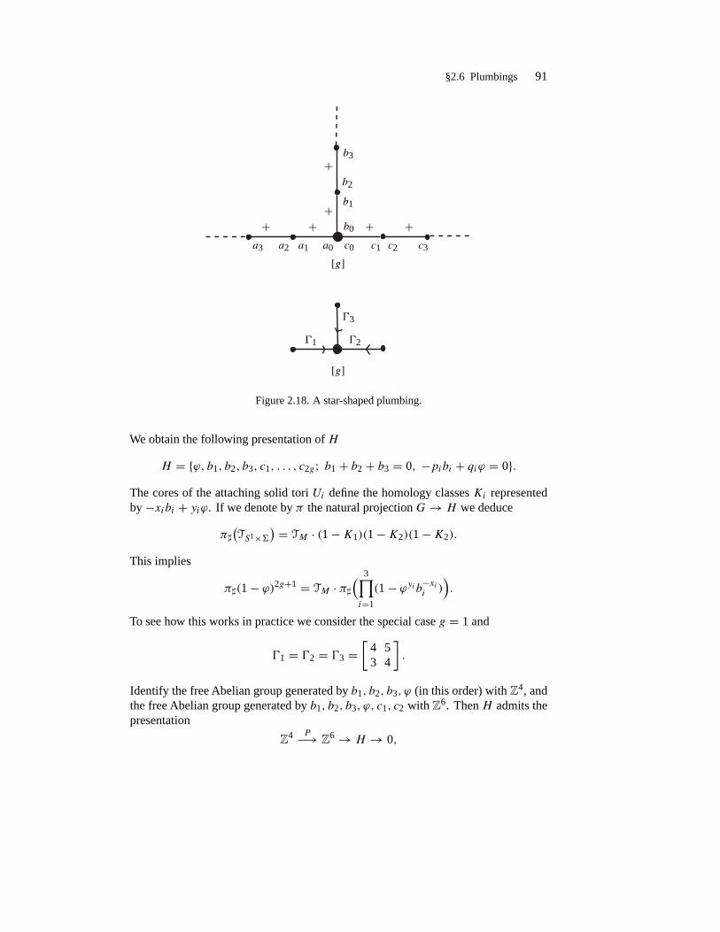
§2.6 Plumbings 91
b3
b2
b1
b0
a3 a2 a1 a0 c0 c1 c2 c3
[g]
[g]
�3
�1 �2
++
+ + +
+
Figure 2.18. A star-shaped plumbing.
We obtain the following presentation of H
H = {ϕ, b1, b2, b3, c1, . . . , c2g; b1 + b2 + b3 = 0, −pibi + qiϕ = 0}.The cores of the attaching solid tori Ui define the homology classes Ki representedby −xibi + yiϕ. If we denote by π the natural projection G→ H we deduce
π�(TS1×�
) = TM · (1−K1)(1−K2)(1−K2).
This implies
π�(1− ϕ)2g+1 = TM · π�( 3∏i=1
(1− ϕyi b−xii )).
To see how this works in practice we consider the special case g = 1 and
�1 = �2 = �3 =[
4 53 4
].
Identify the free Abelian group generated by b1, b2, b3, ϕ (in this order) with Z4, andthe free Abelian group generated by b1, b2, b3, ϕ, c1, c2 with Z6. Then H admits thepresentation
Z4 P−→ Z6 → H → 0,
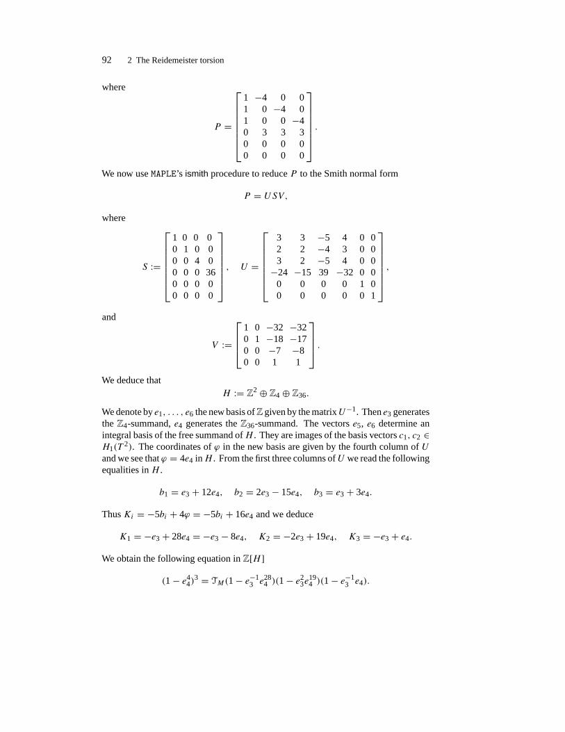
92 2 The Reidemeister torsion
where
P =
1 −4 0 01 0 −4 01 0 0 −40 3 3 30 0 0 00 0 0 0
.
We now use MAPLE’s ismith procedure to reduce P to the Smith normal form
P = USV,where
S :=
1 0 0 00 1 0 00 0 4 00 0 0 360 0 0 00 0 0 0
, U =
3 3 −5 4 0 02 2 −4 3 0 03 2 −5 4 0 0−24 −15 39 −32 0 0
0 0 0 0 1 00 0 0 0 0 1
,
and
V :=
1 0 −32 −320 1 −18 −170 0 −7 −80 0 1 1
.We deduce that
H := Z2 ⊕ Z4 ⊕ Z36.
We denote by e1, . . . , e6 the new basis ofZ given by the matrixU−1. Then e3 generatesthe Z4-summand, e4 generates the Z36-summand. The vectors e5, e6 determine anintegral basis of the free summand ofH . They are images of the basis vectors c1, c2 ∈H1(T
2). The coordinates of ϕ in the new basis are given by the fourth column of Uand we see that ϕ = 4e4 inH . From the first three columns ofU we read the followingequalities in H .
b1 = e3 + 12e4, b2 = 2e3 − 15e4, b3 = e3 + 3e4.
Thus Ki = −5bi + 4ϕ = −5bi + 16e4 and we deduce
K1 = −e3 + 28e4 = −e3 − 8e4, K2 = −2e3 + 19e4, K3 = −e3 + e4.
We obtain the following equation in Z[H ](1− e4
4)3 = TM(1− e−1
3 e284 )(1− e2
3e194 )(1− e−1
3 e4).

§2.6 Plumbings 93
The characters of H have the form χ = ρζz1z2, ρ4 = ζ 36 = 1, z1, z2 ∈ S1. Whenwe Fourier transform the above equation we obtain
(1− ζ−4)3 = TM(ρ, ζ, z1, z2)(1− ρζ 8)(1− ρ2ζ 17)(1− ρζ ),∀ρ4 = ζ 36 = 1, ∀z1, z2 ∈ S1. Observe that
4 · 17 ≡ −4 mod 36, 4 · 8 ≡ −4 mod 36,
so that if we set
ω0 = ω0(χ) = ζ−1, ω1 = ω1(χ) = ρζ 8,
ω2 = ω2(χ) = ρ2ζ 17, ω3 = ω3(χ) = ρζ−1,
then ω40 = ω4
1 = ω42 = ω4
3 and
(1− ω40)
3 =3∏k=1
(1− ω4
k
).
Note that the functions ω40, ωi , i = 1, 2, 3 are precisely the Fourier transforms of
ϕ, [Ki] ∈ Z[H ], i = 1, 2, 3. We conclude
TM(ρ, ζ, z1, z2) ∼
(1−ω4
0)3
(1−ω1)(1−ω2)(1−ω3)if∏3i=1(1− ωi) �= 0
? if∏3i=1(1− ωi) = 0.
(2.23)
To resolve the ambiguity in the last equality we will analyze in greater detail the gluingprocess. Set X := S1 �. We have an inclusion
π : H ↪→ G, G = H1(X).
The functions ω40, ωi : H → S1, i = 1, 2, 3 are restrictions of functions on G, namely
the Fourier transforms of ϕ, [Ki] ∈ Z[G]. We will continue to denote these functionson G by the same symbols as their restrictions to H .
Suppose χ ∈ H is a character such that ωi(χ) = 1, for some i = 1, 2, 3. Thenω4
0(χ) = 1. We now regard χ as a character ofGwith the property χ(ϕ) = 1. In otherwords, χ factors through a character χ of H1(�). As in Example 2.44, the characterχ determines a local coefficient system on � which we denote by Kχ . We can nowuse the Künneth formula for homology with local coefficients, [6], to conclude that
H∗(X,Kχ ) = H∗(S1,C)⊗H∗(�,Kχ ).The groups H∗(�,Kχ ) can be easily determined since � is simple homotopy equiv-alent to a wedge of circles (see Figure 2.19).

94 2 The Reidemeister torsion
c1
c1
c2
c2
b1
b1
b2
b2
Figure 2.19. A cellular Morse decomposition of the torus with three holes.
More precisely, H∗(�,Kχ ) is determined by the based chain complex
C1(c1, c2, b1, b2)∂→ C0(v)→ 0, ∂ci = (zi − 1)v, ∂bi = (βi − 1)v, (2.24)
where zi = χ(ci), βi = χ(bi), i = 1, 2. If we set bk(χ) = dimCHk(�,Kχ ) ande(χ) = b0(χ)− b1(χ)+ b2(χ) then
e(χ) = 3, b2(χ) = 0,
b0(χ) ={
1 if χ = 1
0 if χ �= 1.
We deduce that if χ �= 1 then
dimCH0(X,Kχ ) = dimCH3(X,Kχ ) = 0,
dimCH1(X,Kχ ) = dimCH2(X,Kχ ) = 3.
The manifold M decomposes as an union X ∪ U , where U denotes the union ofthe attached solid tori Ui , i = 1, 2, 3. Denote by V the overlap of these two parts,V = X ∩ U . V is an union of three tori, T1, T2, T3. Fix χ ∈ H \ {1} such that(
1− ω1(χ))(
1− ω2(χ))(
1− ω3(χ)) = 0.
SetIχ := {1 ≤ i ≤ 3; ωi(χ) = 1}.

§2.6 Plumbings 95
We distinguish two cases.
1. |Iχ | < 3. The character χ induces a local coefficient systems on each of theparts X, Ui , Tj , i, j = 1, 2, 3, in the above decomposition of M . Moreover, thelocal coefficient system induced by χ on Ti is trivial if and only if i ∈ Iχ . Thisfollows from the fact that along both Ki , and the attaching curve of the Dehn gluingof Ui the character χ is equal to one. These two curves form a basis of H1(Ti). TheMayer–Vietoris sequence has the form
0 → H3(M,Kχ )→ H2(V ,Kχ )→ H2(X,Kχ )→ H2(M,Kχ )→ · · ·Now observe that
dimCH2(V ,Kχ ) = |Iχ | < 3 = dimH2(X,Kχ ).
This forces H2(M,Kχ ) �= 0 so that TM(χ) = 0 whenever |Iχ | < 3.
2. |Iχ | = 3. In this case the Mayer–Vietoris sequence implies thatH∗(M,Kχ ) = 0 sothat TM(χ) �= 0. To compute the torsion we use the more refined version (1.8) of themultiplicative property of the Mayer–Vietoris sequence. The Mayer–Vietoris sequencefor the homology with local coefficients defined by χ reduces to three isomorphisms
0 → Hk(V,Kχ )φ→ Hk(U,Kχ )⊕Hk(X,Kχ )→ 0, k = 0, 1, 2, (2.25)
where φ is the direct sum �−11 ⊕ �−1
2 ⊕ �−13 ⊕ j , and
j : Hk(V,Kχ )→ Hk(X,Kχ )
is the morphism induced by the inclusion V ↪→ X. We need to fix cellular structureson U,V,X,M such that the attaching maps �i are cellular. On the other hand, asexplained in [72] on smooth manifolds the choice of cellular structure is irrelevantas far as torsion computations are concerned, and we may as well work with cellularcomplexes simple homotopic to the original choices. Next, we need to pick bases inHk(U,Kχ ), Hk(V,Kχ ), Hk(X,Kχ ). Denote by dk(χ), k = 0, 1, 2, the determinantsof the isomorphisms (2.25) with respect to these bases. The cellular structures onX,U ,V , and the bases in the corresponding homologies produce via the Euler isomorphismsscalars
EulV , EulU , EulX ∈ K∗χ .The generalized multiplicative formula now implies that
EulU ·EulX = ±EulV ·TM(χ) · d2(χ)d0(χ)
d1(χ).
Let us now explain how to carry out the computations. Observe first that the restrictionsof the local coefficients system to V andU are trivial. The spacesH0(U),H0(V ) have

96 2 The Reidemeister torsion
canonical bases and since H0(X,Kχ ) = 0 we deduce d0(χ) = 1. Next observe thatH2(U) = 0 and H2(V ) has a canonical basis induced by the orientation.
We denote by C the complex defined in (2.24) and by D the trivial complex
0 → D1 = C 0→ D0 = C→ 0
describing the homology of the fiber of X. We use the based complex C ⊗ D tocompute the twisted homology of X. As basis of H1(�,Kχ ) we choose
{b1, b2, (1− z2)c1 + (z1 − 1)z2}.A quick look at Figure 2.20 shows that (1− z2)c1 + (z1 − 1)c2 = b1 + b2 + b3. Asbasis of H2(X,Kχ ) we choose
{b1 × ϕ, b2 × ϕ, b3 × ϕ}.
z2c1
b1 b2
c2z1c2
b3
c1
Figure 2.20. The twisted homology of the torus with three holes.
We deduce that d2(χ) = 1. We now choose {bi, ϕ} as basis of H1(Ti), i = 1, 2, 3.Since
�−1i =
[4 −5−3 4
]we deduce that
φ(bi) = −3ϕ ⊕ bi ∈ H1(Ui)⊕H1(X,Kχ ),
φ(ϕ) = 4ϕ ⊕ 0 ∈ H1(Ui)⊕H1(X,Kχ ).
We conclude that d1(χ) = ±43. It is easy to check that EulU = ±1 and EulV = ±1.It remains to compute EulX. This can be done using the based complex
0 → A2 = C1 ⊗D1 → A1 = (C0 ⊗D1)⊕ A0 = (C1 ⊗D0)→ C0 ⊗D0 → 0.
Concretely, this is the torsion of the acyclic based complex
0 → H2(X,Kχ )→ A2 ⊕H1(X,Kχ )→ A1 ⊕H0(X,Kχ )→ A0 → 0,

§2.6 Plumbings 97
where Hk(X,Kχ ) is identified with a subspace in Ak . A simple computation showsthat this torsion is ±1. Hence
TM(χ) = ±43.
To determine the torsion we need to use the inverse Fourier transform,
TM =∑
h∈Tors(H)
TM(h)h, TM(h) = 1
4 · 36
∑ρ4=ζ 36=1
TM(ρ, ζ, z1, z2)ρ(h)ζ(h).
The surprising thing about the above formula is that a priori it is not immediatelyclear that the inverse Fourier transform will produce an integer valued function. Wewill present below an elementary argument proving this arithmetic fact directly. Inthe process we will shed additional light on the algebraic structure of the torsion of a3-dimensional Seifert manifolds.
The correspondences χ → ωi(χ) define morphisms Hi → S1, i = 1, 2, 3.We denote by Gi the range of the morphism ωi , and by Zi its kernel. Observethat Z0 := Z1 ∩ Z2 ∩ Z3 coincides with the identity component of H Denote byIZi : H → C the characteristic function of the subset Zi ↪→ H . Set
fi : H → C, fi(ρ, ζ, z1, z2) =3∑k=0
ωki − 4IZi , i = 1, 2, 3.
Observe that
fi(χ) =
1−ω4
i
1−ωi if ωi �= 1
0 if ωi = 1.
This shows that
TM(χ) = f1(χ) · f2(χ) · f3(χ)± 43IZ0 , ∀χ ∈ H .Denote by F −1[•] the inverse Fourier transform. We get
TM =3∏k=1
F −1[fk]
where the above product is the convolution product on C[H ]. Now observe that thePontryagin dual ofGi can be naturally identified with a torsion subgroup of H , moreprecisely the cyclic subgroup generated by [Ki].
F −1[IZi ] = I〈[Ki ]〉.Next observe that
F −1[ω1] = e3e−84 = [K1] ∈ Z[H ],
F −1[ω2] = e23e
194 = [K2] ∈ Z[H ],
F −1[ω3] = e3 · e4 = [K3] ∈ Z[H ].

98 2 The Reidemeister torsion
Hence
TM =3∏j=1
([Kj ] − 4
3∑�=0
[Kj ]�)±
3∏j=1
4( 3∑�=0
[Kj ]�).
The sign ambiguity can be resolved using the Casson–Walker–Lescop invariant ofM ,[58], but we will not get into details. �
Consider a generalized plumbing given by the circular decorated graph at the topof Figure 2.21. Such plumbings arise naturally in the study of cusp singularities (see[45]). Using the concatenation trick we see that this graph is equivalent with theone-loop graph at the bottom of Figure 2.21. This 3-manifold fibers over S1, andthe monodromy is S = �ν . . . �1. Equivalently, this is the mapping torus of thediffeomorphism S : T 2 → T 2. We will denote it by MS . Given this very explicitdescription ofMS we will adopt a direct approach.
�ν
�1 �2
�ν . . . �2�1
Figure 2.21. An arbitrary circular plumbing.
Example 2.58(The torsion of circular plumbings). Denote by�0 the standard latticein R2. We view S as an automorphism of �0 and we denote by �S the sublattice
�S := (1− S)(�0).
From the Wang exact sequence we deduce that we have a short exact sequence
0 → �0/�S → H1(MS)→ Z→ 0.
Now we need to distinguish three cases.
1. S is elliptic, i.e. |Tr S| ≤ 1. There are very few such elements in SL2(Z) and themanifoldMS is very special. More preciselyMS is finitely covered by a 3-dimensionaltorus so that it admits a flat metric. Moreover its diffeomorphism type belongs to avery short list of Seifert fibrations over S2 (see [97, p. 443]). In particular, it can bealternatively represented by a simply connected plumbing graph and the computationis an iterated application of the Mayer–Vietoris principle which we leave to the reader.

§2.6 Plumbings 99
2. S is parabolic, i.e. |Tr S| = 2. For example the plumbing in Figure 2.12 leads to
S = P 41,1 =
[1 40 1
].
In this case MS is an S1-bundle over a torus (see [97, p. 470]) and its Reidemeistertorsion is 1.
3. S is hyperbolic, i.e. |Tr S| ≥ 3. In this case det(1 − S) �= 0, i.e. rank�S =rank(�0) = 2. Fix a splitting of H = H1(MS)
H = GS ⊕ Z, GS = �0/�S.
Observe that S(�S) ⊂ �S so that S induces an action on R2/�S which commuteswith the action of the deck group �0/�S of the cover
�S := R2/�Sπ→ R2/�0 =: �0. (2.26)
We have an explicit description of the universal Abelian cover MS of MS . Moreprecisely
MS = R2/�S × R.The action of (g, n) ∈ GS ⊕ Z = H on MS is given by
(u, n) · (x, t) = (Sn(g · x), t + n) = (g · Snx, t + n), ∀(x, t) ∈ R2/�S × R.Denote by 0 < d1|d2, d1d2 = | det(1 − S)|, the elementary divisors of the sublattice�S . Fix a Z-basis {e1, e2} of �0 such that {d1e1, d2e2} is a basis of �S . We denoteby S0 the matrix representing S with respect to this basis,
S0 :=[a b
c d
],
and set B := 1− S0. Then
d1d2 = | detB| = |TrB| = |2− Tr S0| = |(a − 1)+ (d − 1)|,and d1 = gcd((a − 1), b, c, (d − 1)). Denote byD the 2× 2 matrix diag(d1, d2) andset
S0 := D−1S0D = a d2
d1b
d1d2c d
∈ SL2(Z).
The diffeomorphism S of �0 is described by the matrix S0. It is covered by a diffeo-morphism S of �S described by the matrix S0. S commutes with the action of thedeck groupGS . Note that we can identifyGS with a subgroup of R2/�S and as suchit acts on �S by translations.

100 2 The Reidemeister torsion
Fix n ∈ Z>0 and denote by Fixn the fixed point set of Sn : �0 → �0. For anyx ∈ Fixn the diffeomorphism S defines a permutation of the fiber π−1(x) of the cover(2.26). This fiber is an orbit of the action of GS on �S . Since S commutes with thisaction of GS we deduce that there exists gx ∈ GS such that
Snx = gx · x, ∀x ∈ π−1(x).
Following [32, 33] we define the twisted Lefschetz index of Sn
L(Sn) =∑x∈Fixn
L(Sn, x)gx ∈ Z[GS],
where L(Sn, x) denotes the local Lefschetz index of the fixed point x of Sn. Moreprecisely
L(Sn, x) = sign(1− Sn0 ) = sign(2− Tr Sn0 ) =: εn.It is convenient to write
L(Sn) =∑g∈GS
Lg(Sn)g.
Observe that
Lg(Sn) = 1
|GS |L(Sn − g).
The homeomorphisms Sn and Sn − g of �S are homotopic and using the Lefschetzfixed point theorem we deduce
L(Sn − g) = L(Sn) = 2− Tr(Sn0 ) = 2− Tr Sn0 .
Hence
L(Sn) = L(Sn)IS, IS = 1
|GS |∑g∈GS
g. (2.27)
Define the twisted Lefschetz zeta function
ζ (S) = exp(∑n>0
L(Sn)tn
n
)∈ Q[GS][[t]]. (2.28)
The results in [32, 33] show that the Reidemeister torsion ofMS is equal to the abovetwisted zeta function. To obtain a more explicit description we introduce a new variable
T := ISt.
Since I2S = IS in Q[GS] we deduce that
T n = IStn.

§2.6 Plumbings 101
We can now rewrite (2.28) as
ζ (S) = exp(∑n>0
L(Sn)T n
n
)∈ Q[GS][[T ]].
As shown in Appendix §A.2 the last expression simplifies to
ζ (S) = det(1− T S0)
(1− T )2 = 1− (Tr S0)T + T 2
(1− T )2 = T2 − 2T + 1+ (2− Tr S0)T
(1− T )2 .
If we now recall that |GS | = | det(1 − S0)| = |2 − Tr S0| = |2 − Tr S| and we setSS =∑g∈GS g we can now rewrite the last equality as
TMS = ζ (S) = 1+ sign(2− Tr S)SS
(1− T )2 .
The last quantity belongs to the ring N2(H1(MS)) as predicted by Theorem 2.37. �
Remark 2.59. The computational examples presented in this section conspicuouslyavoided plumbings defining rational homology spheres, i.e. 3-manifolds with finiteH1. These plumbings graphs are trees, and all the vertices have genus zero. In thenext chapter we will deal with this issue in great detail and explain an algorithm forcomputing the torsion of any rational homology 3-sphere. �
Exercise 2.11.Compute the Alexander polynomial of the link in Figure 2.22, andthen compute the Reidemeister torsion of the 3-manifold described by the surgerypresentation indicated in this figure. Compare with the computation in the previousexample. �
−2
−3 0
−5
Figure 2.22. A non-simply connected plumbing.
102 2 The Reidemeister torsion
§2.7 Applications
As mentioned in the introduction, the torsion captures rather subtle topological inter-actions. We will illustrate the strength of this invariant by presenting the classificationsof the 3-dimensional lens spaces.
Recall that L(p, q) is defined as the quotient
L(p, q) := S3/(1,q
where for (r, p) = (s, p) = 1 we denote by (r,s the action of cyclic group Zp on
S3 := {(z1, z2) ∈ C2; |z1|2 + |z2|2 = 1}
defined by the rule
ζ (r,s (z1, z2) = (ζ rz1, ζsz2), ∀ζp = 1.
Observe thatL(p, q) ∼= S3/(k,qk, ∀(p, k) = 1.
This shows immediately that π1(L(p, q)) = Zp so that the integer p is a homotopyinvariant of the lens space. The lens spaces
L(p, q), 1 ≤ q < p, (p, q) = 1
have identical fundamental groups and homology so these classical invariants alonedo not suffice to distinguish them.
Theorem 2.60(Franz–Rueff–Whitehead, [30, 94, 120]). Two lens spaces L(p, q0)
and L(p, q1) are homotopically equivalent if and only if
q0 = ±�2q1 mod p (2.29)
for some � ∈ Z.
Proof. We denote the homotopy equivalences by , .Step 1.
q1 = ±�2q0 mod p *⇒ L(p, q0) , L(p, q1)
For every integers k1, k2 such that (p, ki) = 1 define map fk1,k2 : S3 → S3 by
fk(z1, z2) =(|z1|(1−k1)z
k11 , |z2|(1−k2)z
k22
).
Observe that f has degree k1k2, and it is equivariant, i.e.
fk1,k2
(ζ (r,s (z1, z2)
) = ζ (k1r,k2s (z1, z2).

§2.7 Applications 103
This shows that fk1,k2 induces a map
[fk1,k2 ] : S3/(r,s → S3/(k1r,k2s
of degree k1k2. Fix a point p ∈ S3 and a small ball B centered at p such thatζ k (r,s B ∩ B = ∅, ∀0 < k < p. Set
U =p−1⋃k=0
ζ k (r,s B.
We can equivariantly modify fk1,k2 in U to change its degree by any multiple of p.Suppose for simplicity that q1 = �2q0 mod p. Denote by r0 the inverse of q0 modp. The map f�,�q1r0 is ((1,q0 ,(�,�q1)-equivariant so that it induces a map
[f�,�q1r0 ] : L(p, q0)→ L(p, q1).
We can arrange that deg f�,�q1r0 is any number congruent to �2q1r0 = 1 mod p.In particular, we can arrange so that it has degree 1. Thus f�,�q1r0 induces an iso-morphisms H∗(S3) → H∗(S3). Using the Hurewicz and Whitehead’s theorems wededuce that f is a homotopy equivalence.
Clearly, [f�,�q1r0 ] induces an isomorphism between fundamental groups. Sinceπk(L(p, qi)) = πk(S3), i = 0, 1, k ≥ 2, and the morphisms
[f�,�q1r0 ]∗ : πk(L(p, q0)→ πk(L(p, q1)
)coincide with the morphisms (f�,�q1r0)∗ : πk(S3)→ πk(S
3) which are isomorphismswe deduce from Whitehead’s theorem that f is a homotopy equivalence.
Step 2.L(p, q0) , L(p, q1) *⇒ q0 = ±�2q1 mod p.
To see this we will use the linking form of L(p, q) (see the classical but very intuitive[57, Chap. V] or [99, §77] or the more formal [5, p.366] for details). This is asymmetric, bilinear map
�p,q : H1(L(p, q)
)×H1(L(p, q)
)→ Q/Z
defined as follows. Pick c, d ∈ H1(L(p, q)) represented by smoothly embeddedcircles then pd bounds a 2-chain D which we can represent as an embedded surfacewith boundary pd . Denote by c ·D the (signed) intersection number of c and D andset
�p,q(c, d) := 1
pc ·D mod Z.
Up to a sign, the linking form is a homotopy invariant of the lens space. In fact, wehave (see [99] or Example B.8)
�p,q(ku, ku) = −k2q/p mod Z,
104 2 The Reidemeister torsion
where u is a generator ofH1(L(p, q)). IfL(p, q0) , L(p, q1) the linking forms mustbe isomorphic. Thus there exists generators ui of H1(L(p, qi)) ∼= Zp, i = 0, 1 suchthat u0 = �u1 in Zp and
q0/p = �p,q0(u0, u0) = ±�p,q1(�u1, �u1) = ±�2q1/p mod Z. �
Since ±2 is not a quadratic residue modulo 5 we deduce
L(5, 1) �, L(5, 2).On the other hand, since 2 is a quadratic residue modulo 7 we deduce
L(7, 1) , L(7, 2).The reader can verify easily that two lens spaces L(p, qi), i = 0, 1 such that
q0 = ±q1 or q0q1 = ±1 mod p
are homeomorphic. We can thus parametrize the homeomorphism classes of lensspaces by pairs (p, q) such that
1 ≤ q < p/2, (p, q) = 1. (2.30)
In this list, some spaces are homotopically equivalent, e.g.L(7, 1) , L(7, 2). We willshow that no two lens spaces in this list are homeorphic. In fact, we have the followingresult.
Theorem 2.61(Reidemeister–Franz [29, 90]). If (p0, q0) and (p1, q1) satisfy (2.30)then
TL(p0,q0) ∼ TL(p1,q1) ⇐⇒ (p0, q0) = (p1, q1).
Proof. The implication ⇐* is obvious. Conversely, if TL(p0,q0) ∼ TL(p1,q1) thenclearly p0 = p1 =: p. We have to show that if there exist r ∈ Z, −p/2 ≤ r ≤ p/2and ε ∈ {±1}
(1− ζ )(1− ζ q0) = εζ r (1− ζ )(1− ζ q1), ∀ζp = 1
then q0 = q1. The above identities are equivalent to
1− ζ q0 = εζ r (1− ζ q1)
for all ζp = 1. Assume for simplicity that r ≥ 0. This implies that the polynomial ofdegree < p
P(x) = εxr+q1 − xq0 − εxr + 1.
has p distinct roots. This implies r = 0, ε = 1 and q0 = q1. �
The last result implies that the Reidemeister torsion distinguishes the homeomor-phism types of the homotopically equivalent spaces L(7, 1) and L(7, 2).

§2.7 Applications 105
Remark 2.62. The Hauptvermutung (Main Conjecture) asks if two of homeomorphicsimplicial complexes are necessarily combinatorially equivalent. The answer is knownto be positive for manifolds of dimension≤ 3. In a very beautiful paper [69], J. Milnorhas shown that the Hauptvermutung is false in dimensions ≥ 6. More precisely heconsidered the manifolds with boundary
X1 := L(7, 1)×Dn, X2 = L(7, 2)×Dn, n ≥ 3
and then defined Yi as the (simplicial) space obtained from Xi by adjoining the coneon ∂Xi . He showed that the simplicial spaces Yi are homeomorphic but not com-binatorially equivalent. The relative Reidemeister torsion captures the finer com-binatorial structure. Surprisingly, the absolute torsion is a topological invariant (see[101, 13]) and thus it is blind to the combinatorial structure. A few years later, R. Kirbyand L. Siebenmann (see [101]) have constructed topological manifolds violating theHauptvermutung. �

Chapter 3
Turaev’s refined torsion
In the previous chapter we have defined the torsion of a cell complexX as an elementof Q(H1(X))/±H1(X).
In the beautiful paper [113],Vladimir Turaev has explained the •/H1(X) ambiguityof the torsion in terms Euler structures. In the special case of 3-manifolds, these Eulerstructures are equivalent to spinc-structures. In other words, the Reidemeister torsionof a 3-manifold is rather an invariant of a spinc structure. In this chapter we willsurvey these results of Turaev. We assume the reader is familiar with the basic factsconcerning spin and spinc structures on smooth manifolds, as discussed for examplein [37].
§3.1 Combinatorial Euler structures
Suppose X is a connected, finite simplicial complex. Denote by |X| the associatedtopological space, and by X′ the first barycentric subdivision of X. For each simplexσ of X we denote by [σ ] its barycenter. Form the 0-chain
eX =∑σ∈X(−1)dim σ [σ ] ∈ C0(X
′).
If |X| were a compact, oriented manifold without boundary then, according to [43],eX would be the Poincaré dual of the Euler class ofX. Observe that χ(X) = 0 impliesthat eX is a boundary.
Definition 3.1 (V. Turaev, [113]). Suppose χ(X) = 0.
(a) An Euler chain on X is a singular 1-chain c ∈ C1(|X|) such that
∂c = eX.(b) Two Euler chains c, c′ are called homologous if the chain c − c′ is a boundary.
(c) A combinatorial Euler structure is a homology class of Euler chains . We denoteby Eulc (X) the set of combinatorial Euler structures. �
A special case of Euler chain is a star-shaped 1-chain (suggestively called spiderby Turaev), consisting of a center O ∈ |X|, and paths from O to [σ ] for dim σ evenand paths from [σ ] to O, for dim σ odd (see Figure 3.1). One can prove easily thatany Euler structure is homologous to a spider. If Y is a subcomplex of X such that
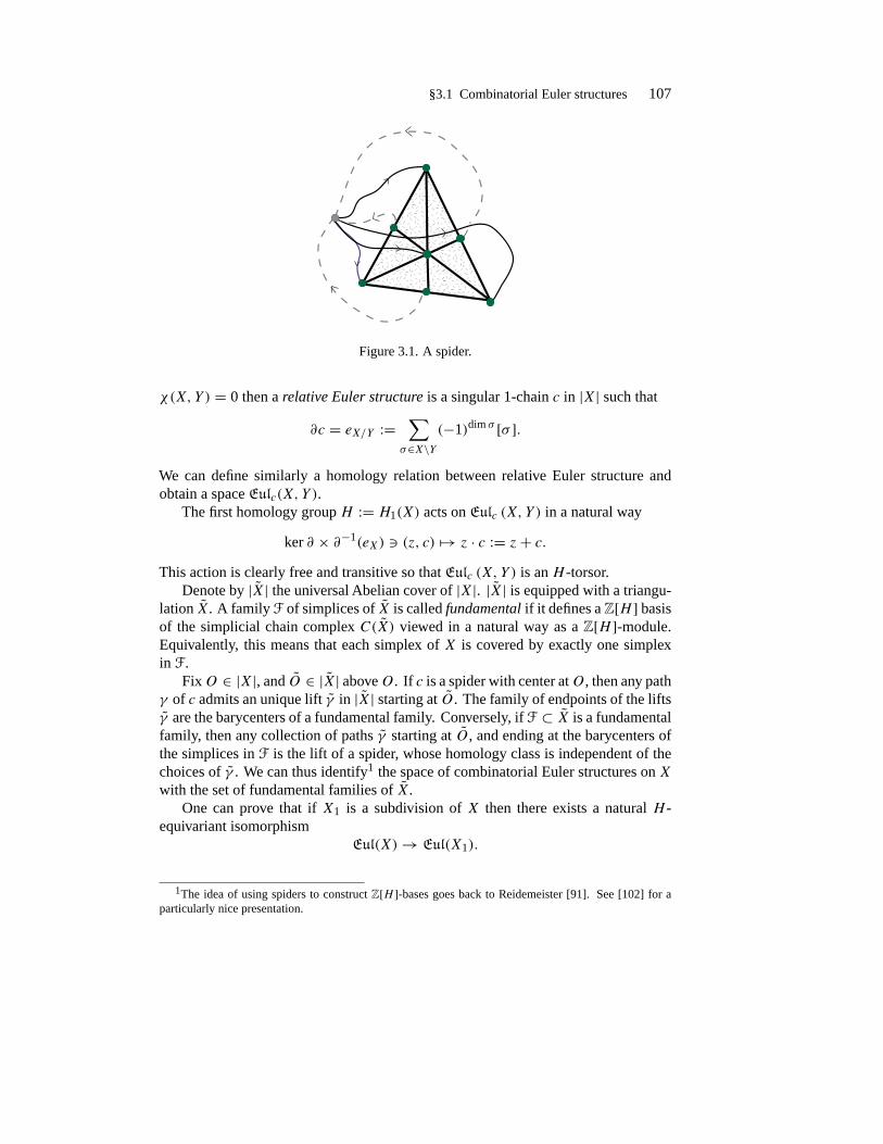
§3.1 Combinatorial Euler structures 107
Figure 3.1. A spider.
χ(X, Y ) = 0 then a relative Euler structure is a singular 1-chain c in |X| such that
∂c = eX/Y :=∑σ∈X\Y
(−1)dim σ [σ ].
We can define similarly a homology relation between relative Euler structure andobtain a space Eulc(X, Y ).
The first homology group H := H1(X) acts on Eulc (X, Y ) in a natural way
ker ∂ × ∂−1(eX) � (z, c) → z · c := z+ c.This action is clearly free and transitive so that Eulc (X, Y ) is an H -torsor.
Denote by ˜|X| the universal Abelian cover of |X|. ˜|X| is equipped with a triangu-lation X. A family F of simplices of X is called fundamental if it defines a Z[H ] basisof the simplicial chain complex C(X) viewed in a natural way as a Z[H ]-module.Equivalently, this means that each simplex of X is covered by exactly one simplexin F.
FixO ∈ |X|, and O ∈ ˜|X| aboveO. If c is a spider with center atO, then any pathγ of c admits an unique lift γ in ˜|X| starting at O. The family of endpoints of the liftsγ are the barycenters of a fundamental family. Conversely, if F ⊂ X is a fundamentalfamily, then any collection of paths γ starting at O, and ending at the barycenters ofthe simplices in F is the lift of a spider, whose homology class is independent of thechoices of γ . We can thus identify1 the space of combinatorial Euler structures on Xwith the set of fundamental families of X.
One can prove that if X1 is a subdivision of X then there exists a natural H -equivariant isomorphism
Eul(X)→ Eul(X1).
1The idea of using spiders to construct Z[H ]-bases goes back to Reidemeister [91]. See [102] for aparticularly nice presentation.

108 3 Turaev’s refined torsion
Exercise 3.1.Prove the above claim. �
Since any two piecewise smooth triangulations of a smooth manifold have a commonsubdivision, the above considerations unambiguously define the space of combinato-rial Euler structures on a smooth manifold.
In the next section we will present a different description of the notion of Eulerstructure on a smooth manifold where the combinatorial structure does not intervene.
§3.2 Smooth Euler structures
Suppose X is a compact, oriented, m-dimensional manifold, possibly with boundary.We assume that the space of components of Y is decomposed into two disjoint parts(possibly empty) and we write this ∂X = ∂+X ∪ ∂−X. It is convenient to think of Xas an oriented cobordism between the two distinguished parts ∂± of its boundary (seeFigure 3.2).
∂−X
X
∂+X
Figure 3.2. An oriented cobordism.
Definition 3.2 (V. Turaev, [113]). A smooth Euler structure on (X, ∂+X, ∂−X) is anowhere vanishing vector field V on X pointing outwards on ∂+X and inwards on∂−X. �
By the Poincaré–Hopf theorem we deduce that smooth Euler structures exist ifand only if χ(X, ∂±X) = 0.
Two smooth Euler structures V , V ′ are called homologous if there exists a closedm-dimensional ball D ⊂ IntM such that the restrictions of V and V ′ to M \ IntDare homotopic as nowhere vanishing vector fields pointing outwards along ∂+X andinwards along ∂−X. (The homotopy can behave arbitrarily along ∂D.) One can verifyeasily that this is an equivalence relation. We denote by Euls(X, ∂+X) the spaceof homology classes of smooth Euler structures on this oriented cobordism. When∂−X = ∅ we write simply Euls(X, ∂X).
It is useful to compare the relation of being homologous with the stronger relationof being homotopic. Consider a cellular decomposition of (X, ∂X)which has a single
§3.2 Smooth Euler structures 109
m-dimensional cell. Given two nonsingular vector fields V , V ′, the first obstructionto them being homotopic is given by an element (see [103])
V/V ′ ∈Hm((X, ∂+X)× (I, ∂I );πm−1(Sm−1))
∼= Hm−1(X, ∂+X)PD∼= H1(X, ∂−X),
where PD denotes the Poincaré duality. This obstruction vanishes if the vector fieldsare homologous. If this happens, there is still a secondary obstruction
δ′(V , V ′) ∈Hm+1((X, ∂+X)× (I, ∂I );πm(Sm−1))
∼= Hm(X, ∂+X;πm(Sm−1)),
where
πm(Sm−1) =
0 m = 2
Z m = 3
Z2 m ≥ 4.
The above discussion shows that we have a well defined map
/ : Euls (X, ∂+X)× Euls (X, ∂+X)→ H1(X, ∂−X), (U, V ) → U/V,
which describes the first obstruction to U being homotopic to V . This operationsatisfies a few elementary properties. (Below we will think of H1(X, ∂−X) as amultiplicative group.)
U/V = 1 ⇐⇒ U = V. (E1)
(U/V ) · (V/W) = U/W. (E2)
∀h ∈ H1(X, ∂X), ∀V ∈ Euls (X, ∂+X),
∃ a unique U ∈ Euls (X, ∂+X) such that h = U/V. (E3)
We will denote by h · V the unique element U postulated by (E3).We have thus obtained a free and transitive action ofH1(X, ∂−X)onEuls (X, ∂+X),
H1(X, ∂−X)× Euls (X, ∂+X) � (h, V ) → h · V ∈ Euls (X, ∂+X).
In particular, if ∂X = ∅, the spaces of combinatorial and smooth structures on(X, ∂+X) must be isomorphic. A little bit later we will prove that there exists acanonical isomorphism between these two spaces of Euler structures. We want topresent an explicit description of the action of H1(X) on Euls(X, ∂+X). Assume∂−X = ∅, so that ∂+X = ∂−X.
Consider an element h ∈ H1(X,Z), and an Euler structure represented by a vectorfield U . Choose an oriented, simple closed curve � representing h and denote by Na tubular neighborhood of � ↪→ IntX. Thus N ∼= Dm−1 × S1 where � = {0} × S1.

110 3 Turaev’s refined torsion
S1 acts in an obvious way by rotations on N , and we denote by )R the infinitesimalgenerator of this 1-parameter group of rotations on N . Also, we denote by )ν theobvious extension toN of the (origin pointing) radial vector field onDm−1 to a vectorfield onN . (Think of )ν as the gradient of the function dg(x) = distg (x, �)where boththe distance and the gradient are computed using a Riemann metric g. This shows thatthe choice of )ν is unique up to a homotopy.) Modulo a homotopy we can assume that
U = − )R on N.
Assuming Dm−1 is the disk of radius π define
V ={U on X \ IntN
cos(r) )R + sin(r))ν on IntN,
where r : Dm−1 → R denotes the radial distance. We call this operation the Reebsurgery along h. In Figure 3.3 we tried to illustrate the differences between the flowofU , on the left, and the flow of V , on the right. Then V/U = h ∈ Hm−1(X, ∂X;Z).To see this notice that given any smooth (m− 1)-cell σ of (X, ∂X) we get a map
f : Sm−1 → Sm−1, f |Sm−1+
= V, f |Sm−1−
= U
such that deg(f ) = #(�∩ σ). The degree of the map f is precisely the obstruction todeforming V |σ to U |σ keeping V |∂σ fixed.
Figure 3.3. Reeb surgery
Remark 3.3. In dimension m = 3 there are countably many possibilities of framingN ∼= D2 × S1, and any two differ by a sequence of Dehn twists. Thus the choice )Rmay not be canonical. However, any two such choices will be homotopic as nowherevanishing vector fields on D2 × S1 because the only possible obstruction lives inH 2(S1×D2;Z) ∼= 0. Thus the Reeb surgery operation is a well defined operation onhomology classes of Euler structures. �

§3.2 Smooth Euler structures 111
Let us observe that the involution U → −U on the space of vector fields inducesa bijection
Euls (X, ∂+X)→ Euls (X, ∂−X).We will denote this bijection by U → U , and we will call this map the conjugation ofEuler structures WhenX is closed the above bijection defines an involution on Eul(X),
Euls(X) � e → e ∈ Euls(X).
For every e ∈ Euls(X) we set
c(e) := e/e ∈ H1(X).
Proposition 3.4. If e ∈ Euls(X) is represented by the nonsingular vector field Uon X then c(e) is the Poincaré dual of the Euler class e(U⊥) ∈ Hm−1(X), wherem = dimX, and U⊥ denotes the (m− 1)-plane sub-bundle of TX orthogonal to U .
Proof. Fix a CW-decomposition ofXwith a singlem-cell. Denote by S1(U⊥) the unit
sphere bundle of U⊥ and by S1(T X) the unit sphere bundle of TX. Set U± = ±Uand denote by V a section of S1(U
⊥) over the (m−2)-skeleton. The section V definesa natural homotopy (see the left-hand side of Figure 3.4)
U : [−1, 1] ×X(m−2)→ S1(T X), (t, x) → Ut (x), U±1 = U±,connecting U− to U+ inside the plane spanned by U± and V .
V
U− t U+ A−1 A0 A1
Ut
Figure 3.4. PD c(e) = e(U⊥).
Suppose σ is an (m− 1)-cell of X with attaching map f : ∂σ → X(m−2) and setY = X(m−2) ∪f σ . Then both U± extend to Y . Set
S = {−1} × σ ∪ [−1, 1] × ∂σ ∪ {1} × σ =: A−1 ∪ A0 ∪ A1.
Fix a trivialization of TX over σ so that we can viewU± as constants maps σ → Sm−1
and V |∂σ as a map V : ∂σ → Sm−2, where we identify Sm−2 to the Equator on Sm−1
perpendicular to U . Now define (see right-hand side of Figure 3.4)
H : S → Sm−1 ={U± on A±1
U on A0.

112 3 Turaev’s refined torsion
Observe that degH is precisely the obstruction to extending the homotopy U over theσ , i.e.
degH = ⟨PD(e/e), σ⟩ = ⟨PD
(c(e)), σ⟩.
On the other hand,H is homotopic to the suspension�V of the map V : ∂σ → Sm−2.By Freudenthal suspension theorem [5, 44] we deduce
degV = deg�V = degH.
Now observe that degV is precisely the obstruction to extending V over σ , i.e.
degV = ⟨PD(c(e)), σ⟩.
This concludes the proof of the proposition. �
Theorem 3.5(Turaev, [113]). Suppose X is a compact, oriented, smooth, m-dimen-sional manifold (possibly with boundary) equipped with a smooth triangulation
(K,L)←→ (X, ∂X).
Assume χ(X, ∂X) = 0. Then there exists a natural H1(X)-equivariant isomorphism
ρ : Eulc(K,L)→ Euls(X, ∂X).
This isomorphism is compatible in a natural way with the barycentric subdivisions.
Proof. We will describe only the construction of ρ. For simplicity, we will do thisonly in the case ∂X = ∅. First we need to introduce a bit of terminology.
Consider a line segment [α, β] ⊂ Rm which we can assume to be of length 3.Denote by V the set of points in R situated at a distance ≤ 1 from this segment butat a distance ≥ 1 from its endpoints α and β; see Figure 3.5. We denote by Dα
Dα
Bα
V Bβ
Dβ
indα = 1
Figure 3.5. A special vector field near a 1-dimensional simplex.
(resp. Dβ ) the closed disk of radius 1 centered at α (resp. β). We set Bα := Dα ∩ V ,Bβ := Dβ ∩ V (see Figure 3.5).
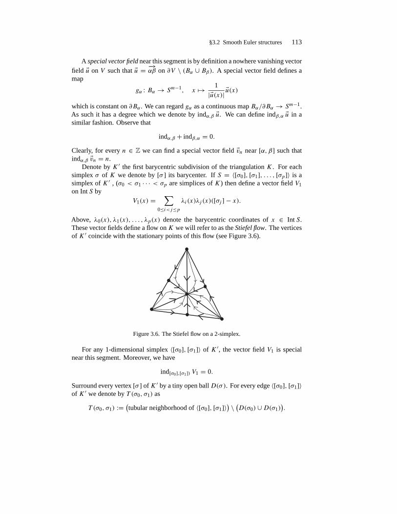
§3.2 Smooth Euler structures 113
A special vector field near this segment is by definition a nowhere vanishing vectorfield )u on V such that )u = −→αβ on ∂V \ (Bα ∪ Bβ). A special vector field defines amap
gα : Bα → Sm−1, x → 1
|)u(x)| )u(x)
which is constant on ∂Bα . We can regard gα as a continuous map Bα/∂Bα → Sm−1.As such it has a degree which we denote by indα,β )u. We can define indβ,α )u in asimilar fashion. Observe that
indα,β + indβ,α = 0.
Clearly, for every n ∈ Z we can find a special vector field )vn near [α, β] such thatindα,β )vn = n.
Denote by K ′ the first barycentric subdivision of the triangulation K . For eachsimplex σ of K we denote by [σ ] its barycenter. If S = 〈[σ0], [σ1], . . . , [σp]〉 is asimplex of K ′ , (σ0 < σ1 · · · < σp are simplices of K) then define a vector field V1on Int S by
V1(x) =∑
0≤i<j≤pλi(x)λj (x)([σj ] − x).
Above, λ0(x), λ1(x), . . . , λp(x) denote the barycentric coordinates of x ∈ Int S.These vector fields define a flow onK we will refer to as the Stiefel flow. The verticesof K ′ coincide with the stationary points of this flow (see Figure 3.6).
Figure 3.6. The Stiefel flow on a 2-simplex.
For any 1-dimensional simplex 〈[σ0], [σ1]〉 of K ′, the vector field V1 is specialnear this segment. Moreover, we have
ind[σ0],[σ1]) V1 = 0.
Surround every vertex [σ ] ofK ′ by a tiny open ballD(σ). For every edge 〈[σ0], [σ1]〉of K ′ we denote by T (σ0, σ1) as
T (σ0, σ1) :=(tubular neighborhood of 〈[σ0], [σ1]〉
) \ (D(σ0) ∪D(σ1)).

114 3 Turaev’s refined torsion
Suppose now thatξ =
∑σ0<σ1
ξ(σ0, σ1)〈[σ0], [σ1]〉
is an Euler chain. We can find a nowhere vanishing vector field Vξ onK \⋃σ<K D(σ)such that the following hold.
• Vξ is special near each segment 〈[σ0], [σ1]〉 , σ0 < σ1, and
ind[σ0],[σ1] Vξ = ξ(σ0, σ1).
• Outside the union of tubes⋃σ0<σ1
T (σ0, σ1) we have
Vξ ≡ V1.
We will show that Vξ extends to a nowhere vanishing vector field on K . This isequivalent to the fact that the induced map
Vξ : ∂D(σ)→ Sm−1
is homotopically trivial, i.e.
d(σ ) := deg(Vξ : ∂D(σ)→ Sm−1) = 0.
Setd0(σ ) := deg
(V1 : ∂D(σ)→ Sm−1).
In [43] it was shown that d0(σ ) = (−1)dim σ . (This identity is intuitively clear inFigure 3.6.) Observe that
d(σ ) = d0(σ )+∑σ<η
(indσ,η Vξ − indσ,η V1)+∑η<σ
(indσ,η Vξ − indσ,η V1)
= (−1)dim σ +(∑σ<η
ξ(σ, η)−∑η<σ
ξ(η, σ )).
On the other hand∑σ
(−1)dim σ [σ ] = ∂ξ =∑σ
(∑η<σ
ξ(η, σ )−∑σ<η
ξ(σ, η))[σ ]
from which it follows that d(σ ) = 0, ∀σ < K . Thus Vξ extends to a nowherevanishing vector field on X. The correspondence
ξ → Vξ
establishes the isomorphism postulated in Theorem 3.5. �
In the sequel we will frequently switch between combinatorial and/or smooth Eulerstructures so that we will drop the subscripts c and s in Eulc/s .

§3.3 U(2) and Spinc(3) 115
Remark 3.6. (a) One can define a notion of Euler structure which combines boththe combinatorial and the differential combinatorial aspects. If X is a closed, com-pact, oriented smooth manifold such that χ(X) = 0, then following [49], we candefine an Euler structure as a pair (V , c) where V is a smooth vector field on X withnondegenerate zero set v−1(0) and c is a smooth 1-chain such that
∂c = v−1(0)
where the zeros of v are weighted by the Poincaré–Hopf signs. The notion of isomor-phism is defined in an obvious way.
(b) One can give a combinatorial description of the conjugation of Euler structure.Suppose X is a smooth, closed oriented manifold such that χ(X) = 0. Fix a smoothtriangulation ofX so we can identifyXwith a polyhedron. Suppose the Euler structuree is represented by the Euler chain c ∈ C1(X). Then the Euler structure e is representedby the Euler chain
c =∑σ0<σ1
(−1)dim σ0+dim σ1〈σ0, σ1〉 + (−1)dimXc.
If we think of combinatorial Euler structures in terms of fundamental families ofsimplices in the universal Abelian cover, then we can give an even simpler descriptionof this involution.
Suppose F is a fundamental family representing the Euler structure e. Then theEuler structure e is represented by the fundamental family F, were F consists of thecells dual to the cells in F. For proofs of these facts we refer to [113, Appendix B]. �
§3.3 U(2) and Spinc(3)
V. Turaev observed in [114] that the space of smooth Euler structures on 3-manifoldscan be identified with the space of isomorphisms of spinc structures. This identi-fication has its origin in some low dimensional representation theoretic “accidents”which we will be discussed in the present section. In the following section we willexplain in detail the connection between spinc structures and smooth Euler structureson 3-manifolds.
Recall that
Spinc(n) ∼= Spin(n)× U(1)/Z2, Z2 ∼= {(1, 1), (−1,−1)} ⊂ Spin(n)× U(1).
In dimension 3 we have an isomorphism Spin(3) ∼= SU(2), and the natural map
SU(2)× S1 � (T , z) → zT ∈ U(2)
descends to an isomorphism Spinc(3) ∼= U(2).
116 3 Turaev’s refined torsion
We want to discuss several facets of this isomorphism. We denote by u(n) the Liealgebra of U(n), su(n) the Lie algebra of SU(n) etc. We begin by presenting a moreexplicit description of the morphism U(2)→ SO(3).
Consider the adjoint representation
Ad : U(2)→ Aut(u(2)).
The diagonal U(1) ↪→ U(2) is the center of U(2) and thus u(2) splits into irreducibleparts
u(2) = u(1)⊕ (u(2)/u(1)).We denote by Ad0 : U(2)→ SO(3) the morphism induced by the above representationof U(2) on the real 3-dimensional space u(2)/u(1).
More explicitly, the space u(2)/u(1) can be identified with the orthogonal comple-ment of δ∗u(1) inside u(2). This complement is precisely su(2). A matrix A ∈ su(2)has the form
A =[
ix z
−z −ix
], x ∈ R, z ∈ C.
From this description we get a natural decomposition su(2) ∼= R ⊕ C. The rep-resentation Ad0 associates to each unitary frame )f := (f 1,f 2) of C2 a matrixAd0( )f ) ∈ Aut(su(2)) as follows. If
f i =[uivi
], ui, vi ∈ C, |ui |2 + |vi |2 = 1, i = 1, 2,
u1u2 + v1v2 = 0.
so that)f :=
[u1 u2v1 v2
]∈ U(2),
then Ad0( )f ) acts on su(2) by
Ad0( )f ) ·[
ix z
−z −ix
]= )f ·
[ix z
−z −ix
]· )f ∗
=[u1 u2v1 v2
]·[
ix z
−z −ix
]·[u1 v1u2 v2
]
= i((|u1|2 − |u2|2)x + 2Im(u1u2z)
)i(u1v1 − u2v2)x + u1v2z− u2v1z
∗ ∗
.Observe that if
)f =[u −vv u
]∈ SU(2)
§3.3 U(2) and Spinc(3) 117
then
)f ·[
ix z
−z −ix
]· )f ∗ =
i(|u|2 − |v|2)x − 2iIm(uvz) 2iuvx + u2z− v2z
∗ ∗
.In particular,
Ad0( )f )[
i 00 −i
]= 2i
12 (|u|2 − |v|2) uv
uv − 12 (|u|2 − |v|2)
.Let us point out that the matrix which appears on the right hand side of the above equal-ity is precisely the quadratic term which enters into the formulation of the Seiberg–Witten equations.
The above description of the morphism U(2) → SO(3) is obviously coordinatedependent. We will now present a coordinate free description of this isomorphism.Suppose now that V is a real, 3-dimensional, oriented, Euclidean vector space. Ob-serve first that, as an SO(V )-module, V is isomorphic to the adjoint representationof SO(V ) on its Lie algebra. (This is a purely 3-dimensional phenomenon.) This isgiven by the correspondence
V � v → Xv := (v × •) ∈ so(V ). (3.1)
Above, “×” denotes the cross product. It can be alternatively defined by
u× v := ∗(u ∧ v),where ∗ is the Hodge operator. By fixing a nonzero vector τ ∈ V we determine severalthings.
•A subgroup Gτ ⊂ SO(V ), the stabilizer of τ with respect to the tautological actionof SO(V ) on V . Gτ is a maximal torus in SO(V ) so that Gτ ∼= S1. The Lie algebraof Gτ is generated by the infinitesimal rotation Xτ in (3.1).
• An action of Gτ ∼= S1 on the orthogonal complement Vτ of τ in V . Thus, Vτ isequipped with a complex structure J , and a Hermitian metric
〈u, v〉 := (u, v)− i(Ju, v),
where (•, •) denotes the Euclidean (real) inner product.
Now form the space
Vτ := R⊕ V ∼=(R⊕ R · τ)⊕ Vτ ∼= C⊕ Vτ .
Vτ is equipped with a complex structure and Hermitian metric which depend on τ .We will construct a representation
ϕτ : U(Vτ )→ SO (Rτ ⊕ Vτ ) = SO (V )

118 3 Turaev’s refined torsion
as follows. Define a vector space isometry
Iτ : V → su(Vτ ), Rτ ⊕ Vτ � (t, φ) → it · ( 〈•, φ〉
− ( ·φ −it · •
.If T ∈ U(Vτ ) then ϕτ (T ) ∈ SO(V ) is defined by the commutative diagram
su(Vτ ) su(Vτ )
V V .
�Ad0(T )
�
Iτ
�ϕτ (T )
�
Iτ
More explicitly, if
T :=[z1 〈•, φ2〉φ1 z2
], zi ∈ C, φi ∈ Vτ ,
then
ϕτ (T )
[t
φ
]= (|z1|2 − |φ2|2)t + 2Im〈z1φ, φ2〉
−it (z1φ1 − z2φ2)+ z1z2φ − 〈φ1, φ〉φ2
.Let us point out a confusing fact. We have produced two U(2)-representations onR⊕ V . The first one is the tautological representation
θ : U(C⊕ Vτ )→ Aut(C⊕ Vτ ),and it is a complex representation. The second one is
1⊕ ϕτ : U(2)→ Aut(R⊕ V ),and it is real. The first representation is the complex spinor representation of Spinc(3)and has (infinitesimal) weights {θ1, θ2}. The second representation is precisely theadjoint representation and its complexification has weights {0, 0,±(θ2 − θ1)}.
We have thus shown that a choice of an unit vector τ ∈ V canonically defines acomplex structure Jτ on R⊕ V and a morphism
U(R⊕ V, Jτ )→ SO(V ).
Let us point out another low dimensional accident.Denote by Herm(V ) the space of hermitian structures on V := R⊕V compatible
with the natural orientation. More precisely,
Herm(V ) = {J ∈ SO(R⊕ V ); J 2 = −1}.

§3.3 U(2) and Spinc(3) 119
Denote by e0 the vector 1⊕ 0 ∈ R⊕ V . One can check that the map
Herm(V ) � J → Je0 ∈ S1(V ) = unit sphere in V,
is a bijection. We denote its inverse by
S1(V ) � τ → Jτ ∈ Herm(V ).
The complex space Vτ is precisely (V , Jτ ). Moreover, ϕτ is a morphism
ϕτ : U(V , Jτ )→ SO(V ).
Finally, we want to explain why the map between classifying spaces
π : BU(2)→ BSO(3)
induced by the morphism Ad0 : U(2)→ SO(3) is a homotopic fibration with homo-topic fiber BS1. We will prove a more general result.
Lemma 3.7. Suppose
1 ↪→ H ↪→ Gφ→ G� 1
is an extension of compact Lie groups. Then the induced map between the correspond-ing classifying spaces
Bφ : BG→ BG
is (homotopically) a fibration with homotopic fiber BH .
Proof.2 Denote by EG → BG (resp. EG → BG) the universal (classifying) G-bundle (resp. G-bundle). The natural projection
EG× EG→ EG
is naturally G-equivariant, where G acts on EG via φ and diagonally on EG× EG.We thus have a map
BG ∼= (EG× EG)/G→ EG/φ(G) ∼= BG.
One can check easily this is a fibration with fiber EG/H ∼= BH . � 2I am indebted to Stephan Stolz for this simple argument.

120 3 Turaev’s refined torsion
§3.4 Euler structures on 3-manifolds
Suppose X is a smooth, compact, oriented 3-manifold. Assume for the purpose ofthis preliminary discussion that ∂X = ∅. Then Eul (X) is an H1(X)-torsor. On theother hand, the space Spinc(X) of isomorphism classes of spinc structures on X is anH 2(X)-torsor. By Poincaré duality we have
H1(X) ∼= H 2(X)
which shows there exist bijections Eul (X) → Spinc(X). In this subsection we willconstruct one such canonical bijection. This will require a fresh look at spinc structures.
As we have explained in the previous section, Spinc(3) ∼= U(2) and
SO(3) ∼= U(2)/U(1),
where U(1) lies inside U(2) as the diagonal subgroup. We denote by Ad0 : U(2)→SO(3) the ensuing morphism.
Definition 3.8. Suppose X is a finite cell complex and P → X is a principal SO(3)-bundle. We define a spinc structure on (X, P ) as a pair (F, α) where F → X is aprincipal U(2)-bundle over X, and α is a surjective, U(2)-equivariant map
α : F → P.
where U(2) acts on P via the morphism Ad0 : U(2)→ SO(3). �
The notion of isomorphism of spinc-structures is obvious. We will denote bySpinc(X, P ) set of isomorphism classes of spinc structures on X.
To obtain a homotopic theoretic description of Spinc(X, P ) we need to use theclassifying spaces B SO(3) and B U(2). The morphism U(2) → SO(3) induces amap
π : BU(2)→ BSO(3)
which is a homotopic fibration with fiber BS1 ∼= CP∞ ∼= K(Z, 2). Since the fiber is2-connected there is only one obstruction to the lifting problem below.
BU(2)
X BSO(3).�
π
������
?
�f
It is given by a three dimensional integral class, the third Stiefel–Whitney classW3(f ) ∈ H 3(X,Z). Two such lifts will be homotopic once they are homotopicover the two skeleton. The obstruction to homotopy is given by a single primaryobstruction in H 2(X,Z). We obtain the following result, very similar in spirit toJ. Milnor’s characterization of spin structure in [71].

§3.4 Euler structures on 3-manifolds 121
Proposition 3.9(Gompf, [40]). Suppose X is a compact CW-complex, and P → X
is a principal SO(3)-bundle. Denote by X(k) the k-skeleton of X. A spinc-structureon P is a U(2) structure on P |X(2) which extends to P |X(3) .
Two spinc-structures (Fi, αi), i = 1, 2 on P are isomorphic if and only if therestrictions of Fi to the 2-skeleton of X are isomorphic as U(2)-bundles. Moreover,the group H 2(X,Z) acts freely and transitively on Spinc(X, P ), i.e. Spinc(X, P ) isnaturally an H 2(X,Z)-torsor.
SupposeY ↪→ X is a subcomplex,P → X is a principal SO(3)-bundle onX, and sis a homotopy class of sections ofP |Y . ThenP defines an SO(3)-bundle [P ] → X/Y .We define a spinc structure on P relative to (Y, s) to be a spinc structure on P inducedby a spinc structure on [P ] via the natural projection X → X/Y . The notion ofisomorphism is the obvious one.
We can provide a more geometric description of the notion of spinc structure.Denote by V the rank 3 real vector bundle P ×ρ R3 where ρ : SO(3) → Aut(R3)
is the tautological representation. Any nowhere vanishing section τ of V defines aspinc-structure on στ on P as follows.
• Form the rank 2-real vector sub-bundle Vτ ↪→ V spanned by the vectors orthogonalto τ . We orient Vτ using the convention
or(V ) = 〈τ 〉 ∧ or(Vτ ).
We have thus equipped Vτ with a U(1)-structure.
• Form the oriented, rank 4 real vector bundle
Vτ = R⊕ V ∼= R⊕ 〈τ 〉 ⊕ Vτ .The above decomposition equips Vτ with a complex structure defining a principalU(2)-bundle FV = Fr (Vτ ) → X. As explained in §3.3, the vector field τ defines alift
ϕτ : Fr (Vτ )→ Fr (V ) = Pwhich is the spinc structure associated to the vector field τ . We denote it by στ . Theassociated bundle of complex spinors is the complex bundle Vτ and it has determinantline bundle Vτ . We denote it by det(σ ) = det(στ ). Observe that if h ∈ H 2(X) andσ ∈ Spinc(X, P ) then
det(h · σ) = det(σ )+ 2h, (3.2)
whereH 2(X)× Spinc(X, P ) � (h, σ ) → h · σ ∈ Spinc(X, P )
denotes the action of H 1(X) on Spinc(X, P ), and we have used the identificationbetween complex line bundles on X and H 2(X) given by the (integral) first Chernclass.
The discussion at the end of §3.3 shows that a choice of spinc structure is equivalentto a choice of a nowhere vanishing section of TX. Two choices of such sections lead
122 3 Turaev’s refined torsion
to isomorphic spinc-structures if and only if they are homotopic over the two skeletonof X.
Exercise 3.2.Formulate and prove the counterparts of the above statements for rela-tive spinc structures. �
In the special case whenX is a closed, oriented three manifold such thatχ(X) = 0,and V ∼= TX we deduce that the correspondence
nowhere vanishing vector field τ on X→ στ ∈ Spinc(X)
induces a bijectionEul (X)→ Spinc(X), e → σe.
Proposition 3.4 implies thatPD c(e) = det(σe).
The above discussion also shows that the above map is H 2(X,Z)-equivariant.Finally, we can equivalently describe a spinc-structure as an elementu ∈ H 2(FrX),
FrX := the principal bundle of oriented orthonormal frames of TX, whose restrictionto each fiber is a generator of H 2(SO(3)) ∼= Z2. The correspondence between thesetwo descriptions is clear.
A nowhere vanishing section τ of TX defines a trivial complex line sub-bundle ofthe rank two complex vector bundle Vτ := 〈τ 〉 ⊕ TX. We thus obtain a trivial U(1)sub-bundle of F = Fr
Vτ. We then construct the line bundle
Lτ := F → F/U(1)τ∼= FrX .
Then the class u := c1(Lτ ) ∈ H 2(FrX) restricts to the generator on each fiber.In terms of the second interpretation, the action ofH 2(X,Z) on Spinc(X) has the
descriptionx · u = π∗Xx + u, u ∈ H 2(FrX), x ∈ H 2(X),
where πX : FrX → X is the natural projection. (The above action of H 2(X) onH 2(FrX) obviously preserves Spinc(X) ⊂ H 2(FrX).)
The group of orientation preserving diffeomorphisms ofX induces a natural actionon Eul (X), and thus an action on Spinc(X).
The case of 3-manifolds with boundary deserves special consideration. SupposeX is a compact, oriented 3-manifold with boundary ∂X a union of 2-tori. Let usnow point out the remarkable fact that the tangent bundle of a torus S has a canonicalframing induced by an arbitrary diffeomorphism
φ : S → S1 × S1.
Exercise 3.3.Prove that the homotopy class of the framing of T S described above isindependent of the diffeomorphism φ : S → S1 × S1. �

§3.4 Euler structures on 3-manifolds 123
The restriction of the SO(3) bundle TX to the boundary ∂X has a canonicaltrivialization induced by the outer normal section
)ν : ∂X→ TX|∂X,and the canonical framing of T ∂X. We can thus define spinc structures onX relative to∂X and the above canonical framing of TX|∂X. The notion of relative spinc structurecan be given a more geometric description.
Fix for convenience a Riemann metric g on X and denote by )n the unit outernormal. Recall that R denotes the trivial real line bundle over a (generic) space.Observe that the rank 4- vector bundle
V0 :=(R⊕ TX)|∂X ∼= (R⊕ 〈)n〉)⊕ T ∂X,
is canonically a trivialized U(2)-bundle. We denote by J0 the complex structure onV0. A relative spinc structure is then a U(2)-structure J on V := R ⊕ TX togetherwith an isomorphism φ : V |∂X → V0. Two relative spinc structures σi := (Ji, φi),i = 0, 1 are called isomorphic if there exists an isomorphism � : (V , J0)→ (V , J1)
which makes the following diagram commutative.
(V , J0)|∂X (V, J1)|∂X
(V0, J0).
��
���φ0
φ1
The space Spinc(X, ∂X) of isomorphism classes of relative spinc structures is naturallyan H 2(X, ∂X)-torsor. We have an obvious H 2(X, ∂X) map
Eul(X, ∂X)→ Spinc(X, ∂X), e → σ(e),
which must be an isomorphism. The group of orientation preserving diffeomorphismsof (X, ∂X) acts naturally Eul(X, ∂X), and thus on the space of relative spinc-structuresas well.
For any σ = (V , J ) ∈ Spinc(X, ∂X), the determinant line bundle det(σ )|∂X isequipped with a canonical nowhere vanishing section so that we have a well definedclass
c1(det(σ )) ∈ H 2(X, ∂X).
The identity (3.2) shows that the map
c : Spinc(X, ∂X)→ H 2(X, ∂X), σ → c(σ ) := c1(det σ)
is one-to-one if H 2(X, ∂X) has no 2-torsion.
Example 3.10. Suppose X is the solid torus S1 × D2. The relative spinc-structuresσ on X are uniquely determined by
c(σ ) := c1(det σ) ∈ H 2(X, ∂X) ∼= H1(X) ∼= Z.

124 3 Turaev’s refined torsion
Denote by (r, θ) the polar coordinates on D2 and by ϕ the angular coordinate on S1.Consider the nowhere vanishing vector field V on X defined by
V (r, θ, ϕ) := cos(πr/2)∂ϕ + sin(πr/2)∂r .
The vector field sin(πr/2)∂r−cos(πr/2)∂ϕ is a section ofV ⊥which vanishes transver-sally exactly along the core of the solid torus. Thus, if σV denotes the relative spinc
structure determined by V then
cσV = ±[C] ∈ H1(X)
where [C] denotes the oriented core, i.e. the cycle S1 × {0} ∈ X. We deduce that forany spinc structure σ ∈ Spinc(X, ∂X) we have
c(σ ) = (2n+ 1)[c], n ∈ Z.The canonical spinc structure on the solid torus is the spinc structure σcan uniquelydetermined by the condition
c(σcan) = −[C]. �
Example 3.11. Suppose
X = I × S1 × S1, I = [−1, 1].We can regard it as a trivial cobordism between ∂−X := {−1} × T 2 and ∂+X :={1} × T 2. The longitudinal vector field ∂t induces a canonical spinc structure σ0 ∈Spinc(X, ∂+X).
On the other hand, we can regardX as a 3-manifold with (disconnected) boundary∂X. The space Spinc(X, ∂X) is an H1(X) = Z2-torsor. Since H1(X) ∼= H 2(X, ∂X)
has no 2-torsion we deduce that the map
Spinc(X, ∂X) � σ → c1(det(σ )) ∈ H 2(X, ∂X) ∼= Zis one-to-one. Hence, in this case a relative spinc-structure is uniquely specified bythe associated determinant line bundle.
Observe first that the image of Spinc(X, ∂X) in Z2 via the above map is
ε + 2Z, )ε ∈ Z2.
We claim that )ε = 0. To see this, frame TX using the moving frame
(e1, e2, e3) := (∂t , ∂θ1 , ∂θ2).
Now define �0 ∈ Vect (X) by
�0(t, θ1, θ2) = sin(πt/2)e0 + cos(πt/2)e1.
§3.4 Euler structures on 3-manifolds 125
Clearly �0 points outwards on ∂X. Moreover, the vector e2 defines a nowhere vanish-ing section of 〈�0〉⊥. This shows that the relative spinc structure induced by �0 hastrivial determinant and thus )ε = 0.
We will denote by σ0 the spinc structure induced by �0 and we will refer to it asthe trivial spinc structure on the trivial cobordism. �
The vector field �0 constructed in the above example has the following obviousuniversality property.
Lemma 3.12. Suppose X is an oriented 3-manifold with boundary an union of tori.Fix a tubular neighborhood U of ∂X ↪→ X of the form [−1, 1] × ∂X oriented suchthat ∂t is the outward pointing longitudinal vector field. Then any nowhere vanishingvector field V pointing outward on ∂X is homologous to a vector which coincides with�0 along U .
Fix a tubular neighborhood U of ∂X as in the above lemma. Suppose V is anowhere vanishing vector field on X which is equal to ∂t along U . Define the vectorfield V by
V ={−V in X \ U�0 in U.
This operation induces an involution
Eul(X, ∂X)→ Eul(X, ∂X), e → e.
Proposition 3.13. Let e ∈ Eul(X, ∂X). Then
e = c(σ (e)) · ei.e. c(σ (e)) = c(e/e).
Exercise 3.4.Prove the above result. �
The conjugation operation on Euler structure translates to an involution
Spinc(X, ∂X)→ Spinc(X, ∂X), σ → σ .
Suppose now that a closed, oriented 3-manifoldX is decomposed into two, manifoldswith boundary by an embedded torus (or union of tori) �,
X = X0 ∪X1, ∂Xi ∼= (−1)i�, i = 0, 1.
126 3 Turaev’s refined torsion
Fix a tubular neighborhoodU of� ↪→ X which is orientedly diffeomorphic to I ×�.Enlarge
Xi → Xi := Xi ∪ I ×�, i = 0, 1.
Any nowhere vanishing vector field Vi on Xi which points outwards on ∂Xi can beassumed to coincide with �0 on U = I ×� ⊂ Xi , i = 0, 1. Thus
V0 = V1 on I ×� = X0 ∩ X1,
so that we can form the glued vector field on X
V := V0#V1.
It is easy to see that this induces a map
# : Eul (X0, ∂X0)× Eul (X1, ∂X1)→ Eul (X).
This pairing is not necessarily injective and/or injective. We will refer to this pairingas the gluing operation.
§3.5 The Reidemeister–Turaev torsion of Euler structures
SupposeX is a connected, finite simplicial complex such that χ(X) = 0. Fix p0 ∈ X.Set H := H1(X) and denote by
π : X→ X ∼= X/Hthe universal Abelian cover. Fix p0 ∈ X covering p0.
Pick now an Euler structure e ∈ Eul (X) which we can represent by a spider scentered at p0. s admits a unique lift to a spider s on X centered at p0. The 0-chain ∂ sdepends only on the homology class of the spider s, i.e. only on the Euler structure e!Every point q ∈ ∂ s is the barycenter of a simplex cq of the triangulation of X inducedby the triangulation of X. It is clear that if q1 �= q2 then cq1 and cq2 do not cover thesame simplex of X. This means that the collection
ce ={cq; q ∈ ∂q
}is a geometric basis of the Z[H ]-module C(X), and we can now define
TX,e,p0 := T(C(X), ce, p0) ∈ Q(H)/± 1.
The ±1 is due to the multiple choices of orderings/orientations of c. Moreover, sinceχ(X) = 0 we can see that TX,e,p0 is independent of p0. Thus, we can use the notation

§3.6 Arithmetic properties of the Reidemeister–Turaev torsion of 3-manifolds 127
TX,e. We will call it the Reidemeister–Turaev torsion of the Euler structure e. Observethat
TX,h·e ≈ h · TX,e, ∀h ∈ H, e ∈ Eulc(X).
Above, “≈” denotes the equality in Q(H)/± 1.This refined torsion was defined in terms of a simplicial structure on X. One can
prove, much like in the un-refined situation, that this torsion is invariant in an obvioussense under subdivisions and simple homotopy equivalences. For details we refer to[113, §3,4].
One can get rid of the±1 ambiguity by ordering and orienting the simplices ofX.A choice of ordering and orientations on c clearly induces an ordering and orientationon any lift ce. An equivalence class of orderings and orientations of the simplices ofX is completely determined by an orientation of the homology space H∗(X,R). Thiscan be seen using the Euler isomorphism
Eul : Det(C∗(S(X))⊗ R→ Det(H∗(X,R)).
We define a homology orientation on a simplicial complex X to be a trivialization ofthe determinant line Dets H∗(X,R). Fix a homology orientation o. For any geometricbasis c of C∗(X) we define as in Remark 2.40.
ε(c, o) = sign Eul(det(c)) ∈ Det(H∗(X,R)) ∼= R.If c is a geometric basis of C∗(X) and s is a spider representing a fixed combinatorialEuler structure e, then we get a geometric basis cs of the Z[H1(X)]-module C∗(X)which covers c. We use this basis to compute the torsion, and we define the sign-refinedtorsion of (X, e) to be
TX,e,o := ε(c, o)T(C∗(X), cs).
This quantity is independent of the geometric basis c. The relative Reidemeister–Turaev torsion is defined in a similar way (see [113, 117]).
§3.6 Arithmetic properties of the Reidemeister–Turaev torsionof 3-manifolds
This section is a refinement of §2.4 where we proved several arithmetic propertiesof the torsion of 3-manifolds. We take-up this subject again, emphasizing the newaspects due to the sign, and spinc-refinements introduced in the previous section. Formore information, and details we refer to [114, 116] which served as our main sourcesof information.
Denote byX+ the collection consisting of triplets (M, σ, o) satisfying the followingconditions.

128 3 Turaev’s refined torsion
•M is a compact, smooth, oriented 3-manifold, possibly with boundary consisting ofan union of tori.• σ ∈ Spinc(M, ∂M).• o is an enhanced homology orientation. This means that if b1(M) �= 1, then ois an usual homology orientation, and if b1(M) = 1, then o is an orientation of theone-dimensional real vector space H1(M,R).
We denote by X+1 the subfamily of X+ consisting of manifolds with positive b1.
Remark 3.14. A closed oriented 3-manifold admits a natural homology orientationdefined by the Poincaré duality. Similarly, the complement of an oriented link in arational homology sphere admits a natural homology orientation (see [116, §3]) fordetails. In the sequel if an admissible manifold is either closed or it is the complementof a link in a rational homology sphere we will tacitly assume it is equipped with thenatural orientation, unless indicated otherwise. �
For (M, σ, o) ∈ X+ we denote by TM,σ,o ∈ Q(H1(M)) the sign refined Reide-meister–Turaev torsion of the pair (M, ∂M) and the Euler structure σ . It satisfies thefollowing properties.
TM,h·σ,o ≈ hTM,σ,o, h ∈ H1(M), σ ∈ Spinc(M, ∂M), (3.3)
where we recall that ≈ denotes equality up to a sign. In particular
TM,σ,o ≈ TM,σ ,o = c(σ /σ )TM,σ,o = c(σ )−1TM,σ,o. (3.4)
We can be much more precise about the signs in the above formula. More precisely,we have (see [113, Appendix B], [116, Appendix 3])
TM,σ,o = (−1)b0(∂M)TM,σ ,o = (−1)b0(∂M)c(σ )−1TM,σ . (3.5)
Example 3.15. We have defined the canonical spinc structure σcan on the homologi-cally oriented solid torus Z = D2 × S1 with axis K = {0} × S1 by the equality (seeExample 3.10)
c(σcan) = K−1 ∈ H1(Z).
The torsion of the canonical spinc structure σcan is then
TZ ≈ (1−K)−1. �
Remark 3.16. SupposeM is closed (and equipped with the canonical homology ori-entation). We denote by Spin(M) the space of isomorphism classes of spin structuresonM . It is naturally an H 1(M,Z2)-torsor. There exists a natural map
Spin(M)→ Spinc(M), Spin(M) � ε → σ(ε) ∈ Spinc(M).

§3.6 Arithmetic properties of the Reidemeister–Turaev torsion of 3-manifolds 129
Its image consists exactly of the fixed points of the involution σ → σ on Spinc(M).For every spin structure ε onM we set
TM,ε := TM,σ(ε) ∈ Q(H).The symmetry properties (3.4) and (3.5) imply
TM,ε = TM,ε, ∀ε ∈ Spin(M).
WhenM is a rational homology sphere the map ε → σ(ε) is an injection. �
To list the other properties of the sign-refined Reidemeister–Turaev torsion we needto discuss separately several cases. LetM,σ, o) ∈ X+, and set H := H1(M).
A. b1(M) ≥ 2. We already know that TM,σ,o ∈ N2[H ] (see §2.4).
B. b1(M) = 1. Here we distinguish two subcases.
B.1. ∂M = ∅. We already know that TM,σ ∈ N2(H) (see §2.4). We can be muchmore precise. The orientation o on H1(M,R) defines a bijection H/TorsH → Z,and thus a surjection
dego : H → Z.
Fix an element T ∈ H such that dego T = 1. As in §1.5 we set
SH :=∑
h∈Tors(H)
h ∈ Z[H ].
Then (see [114, §4.2])
TM,σ + dego(c(σ ))+ 2
2(1− T )−1SH − (1− T )−2SH ∈ Z[H ]
Suppose that σ = σ(ε), ε ∈ Spin(M). Then dego(c(ε)) = 0, and the above equalitytakes the form
TM,ε,o − T
(T − 1)2SH ∈ Z[H ].
Set deg+o := max(deg, 0), and define
WM :=∑h∈H
deg+o (h−1)h = T
(T − 1)2SH ∈ Q(H), T 0
M,ε = TM,ε −WM.
Observe thatWM = WM
which implies that T 0M,ε is an element of Z[H ] symmetric with respect to the conju-
gation in Z[H ]. We will refer to T 0M,ε as the modified Reidemeister–Turaev torsion
130 3 Turaev’s refined torsion
of M . It is independent of the orientation of H1(M,R) For reasons which will be-come apparent in §4.1, we will refer to WM as the wall crossing term defined by theorientation of H1(M,R). Thus
TM,ε,o = T 0M,ε,o +WM. (3.6)
We set�M,ε,o := (1− T )2 TM,ε,o ∈ Z[H ].
As our choice of notation suggests, one should think of �M,ε,o as a refined versionof the Alexander polynomial of M . This intuition agrees with the identities in Theo-rem 2.37. We deduce from the equality (3.6) that
�M,ε,o = (1− T )2 T 0M,ε + TS.
If we take the Fourier transform of the above equality we deduce
�M,ε(1) = |TorsH |which is precisely the Alexander formula.
B.2. ∂M = S1 × S1. In this case M can be viewed as the complement of a knot ina rational homology sphere. An orientation of the knot induces a natural homologyorientation. In this case Hk(M) = 0 for k > 1 and the homology orientation definesas above a surjection degoH → Z. Choose an element T such that dego T = 1. Then(see [114, §4.2])
TM,σ,o − (1− T )−1SH ∈ Z[H ]. (3.7)
In particular, this implies TM,σ ∈ N1(H) as established in Theorem 2.35.
C. b1(M) = 0. Thus ∂M = ∅ and we know that TM,σ ∈ N(H). In terms of Fouriertransform this means that
TM,σ (1) = 0.
This time TM,σ �∈ Z[H ] but the torsion still has some extra arithmetical properties.More precisely, if o0 is the canonical homology orientation, then (see [114])
TM,σ,o0(g − 1)(h− 1) = − lkM(g, h) mod Z, ∀g, h ∈ H1(M), (3.8)
where lkM : H1(M) × H1(M)→ Q/Z is the linking form of the rational homology3-sphereM .
Observe that if (M, σ, o) ∈ X+, then any orientation preserving diffeomorphismf ofM induces a new enhanced homology orientation f ∗o and a new spinc structure.Define ε(f ) ∈ ±1 by the equality f ∗o = ε(f )o. Then
TM,f ∗σ,f ∗o = ε(f )c(f ∗σ/σ)f∗(TM,σ,o
). (3.9)

§3.7 Axiomatic description of the Reidemeister–Turaev torsion of 3-manifolds 131
§3.7 Axiomatic description of the Reidemeister–Turaev torsionof 3-manifolds
Denote by X the collection consisting of pairs (M, σ) satisfying the following condi-tions.
•M is a compact, smooth, oriented 3-manifold, possibly with boundary consisting ofan union of tori. We will refer to such a manifold as admissible.• σ ∈ Spinc(M, ∂M).
We denote by X1 the subfamily of X consisting of manifolds with positive b1.We summarize the results established so far. The Reidemeister–Turaev torsion is aninvariant
X � (M, σ) → TM,σ ∈ Q(H1(M)
)/± 1
satisfying the following properties.
Axiom 0. Integrality.
TM,σ ∈{
N2[H ] if ∂M = ∅N1[H ] if ∂M �= ∅, ∀σ ∈ Spinc (M, ∂M).
Axiom 1. Topological invariance. The map
TM,• : Spinc (M, ∂M)→ N[H ]/± 1, σ → TM,σ ,
is H1(M)-equivariant, and moreover, if f : M → M ′ is an orientation preservingdiffeomorphism then
TM,f ∗σ ′ ≈ c(f ∗σ/σ)f∗(TM ′,σ ′
).
Axiom 2. Excision. SupposeM is an admissible 3-manifold, and L = L1 ∪ · · · ∪Lnis an oriented link in M such that [L1], . . . , [Ln] have infinite orders in H1(M). (Inother words,M is the result of a nondegenerate Dehn surgery.) Denote by Zi a small,open tubular neighborhood of Li ↪→ M and set
E := M \( n⋃i=1
Zi
).
Denote by σi the canonical spinc structure on the solid torus. Then, the elements(1 − [Li]) are invertible in N1
(H1(M)
)(cf. Lemma 2.42 in §2.5), and for every
σ ∈ Spinc(E, ∂E) we have
TM,σ#σ1#...#σn ≈i#(TE,σ)∏n
i=1
(1− [Li]
) ,

132 3 Turaev’s refined torsion
where i : H1(E)→ H1(M) denotes the inclusion induced morphism.
Axiom 3. Normalization. Suppose L ↪→ S3 is a link with at least two components.Denote by E the exterior of E. Then for every σ ∈ Spinc(E, ∂E) the torsion TE,σ isa representative of the Alexander polynomial of the link E, i.e.
TE,σ ∼ �L,where we recall (see page 45) that ∼ denotes the equality in N2(H)/ ± H , while ≈denotes the equality in N2(H)/± 1.
Suppose H is a finitely generated Abelian group of rank ≥ 1. In §1.5 we haveidentified N2(H) with a ring of functions
f : H → Z
with semi-infinite support, with multiplication given by the convolution product. Forevery f ∈ Z[[H ]] we can define
supp(f ) := {h ∈ H ; f (h) �= 0}.Observe that if (M, σ0) ∈ X we define
supp(M) := {σ ∈ Spinc(M, ∂M); σ := h · σ0, h ∈ supp TM,σ0
}= {σ ∈ Spinc(M, ∂M); 0 ∈ supp(TM,σ )
}.
Clearly, supp(M) is independent of the initial choice σ0 ∈ Spinc(M, ∂M). Thegroup�M of isotopy classes of orientation preserving diffeomorphisms ofM preservesSpinc(M, ∂M) and Axiom 1 implies that supp(M) is �M invariant. This is a verypowerful restriction when b1(M) ≥ 2 because in this case
TM,σ ∈ Z[H ]so that supp(M) is a finite �M -invariant subset of Spinc(M, ∂M).
Theorem 3.17(Uniqueness Theorem; Turaev [115]). If#1, #2 are two invariants onX1 satisfying the above axioms then
#1 ≈ #2.
Proof. Let us first observe that if H is a finitely generated Abelian group of rank ≥ 1then an element U ∈ N(H) is trivial if and only if there exists a non-torsion class hsuch that
(1− h)U = 0.
Define as above supp#i (M) ⊂ Spinc(M, ∂M) for any admissibleM and set
Y := {(M, σ) ∈ X1; #1(M, σ) ≈ #2(M, σ)},

§3.7 Axiomatic description of the Reidemeister–Turaev torsion of 3-manifolds 133
Y′ := {(M, σ) ∈ X1; #1(M, σ) ∼ #2(M, σ)}.
Clearly Y ⊂ Y′.The normalization axiom implies that Y′ contains the complements of links in S3
with at least two components. Moreover, the H1(M)-equivariance implies
(M, σ) ∈ Y (respectively Y′) ⇐⇒ (M, σ ′) ∈ Y (respectively Y′),
∀σ ′ ∈ Spinc(M, ∂M). For this reason, we will say thatM ∈ Y (or Y′) if (M, σ) ∈ Y(or Y′ ) for some σ .
Since any admissible 3-manifold can be obtained by a nondegenerate Dehn surgerywe deduce from the excision axiom that Y′ contains all the admissible manifolds. Atthis point however, it is not even clear that Y �= ∅. The uniqueness theorem isequivalent to the equality Y′ = Y whose proof will be carried out in several steps.
Step 1.I × S1 × S1 ∈ Y.
Step 2.D2 × S1 ∈ Y.
Step 3. If K1, . . . , Km, m ≥ 2 are disjoint unknots in S3 such that
Lk (K1,Km) �= 0, ∀i = 2, . . . , m
then the exterior of the link L = ∪iKi belongs to Y.
Step 4. The exterior of any weakly trivial link in S3 in Y. (A link is called weaklytrivial if its components are unknots.)
Step 5.The exterior of any link in S3 is in Y.
Step 6.Y′ = Y.
The proof of Step 1 is based on the observation that I × S1 × S1 is the exterior Eof the Hopf link in S3. Moreover, using Axiom 3 we deduce supp#i (E) consists of asingle σi ∈ Spinc(E, ∂E) which must be �E-invariant. There is only one such Eulerstructure, namely the trivial one constructed in Example 3.11. Using Step 1 and theexcision axiom we deduce that if K denotes the core of a solid torus X = D2 × S1
then (1− [K])#1(X) ≈ #1(X \K) ≈ #2(X \K) ≈
(1− [K])#2(X),
so that (1− [K])(#1(X)±#2(X)
) = 0, #i(X) ∈ N2(H1(X)).
Thus #1(X) ≈ #2(X), and this completes Step 2.Step 3 follows by induction on the number m of components. The case m = 1
is covered by Step 2. We assume the claim is true for k < m and we prove it forlinks with m components. Denote by E the exterior of a link L = ⋃mi=1 Li with mcomponents such that Lk (L1, Lj ) �= 0, ∀j �= 1. Let us first show that #1(L) �= 0.Denote byM the complement of L1 in S3. Then we can regard E as the complement

134 3 Turaev’s refined torsion
of L2 ∪ · · · ∪ Lm in M . Since Lk(L1, Li) �= 0 we deduce that Li determines anontrivial homology class in H1(M). If #1(E) = 0 then the excision axiom wouldimply #1(M) �= 0 which we know is not the case.
Fix σ0 ∈ Spinc(E, ∂E). Since E ∈ Y′, there exists g ∈ H1(E) such that
#1(E, σ0) = εg#2(E, σ0), ε = ±1.
From the H1(E)-equivariance we deduce
#1(E, σ ) = εg#2(E, σ ), ∀σ ∈ Spinc(E, ∂E).
g is uniquely determined by the above equality since #1(E) �= 0. Denote by µi anoriented meridian of Li . The cycles µi form a basis of H1(E) and thus we can write
g =m∏i=1
µkii , ki ∈ Z.
We can now conclude by gluing back to E the tubular neighborhood of Li , i > 1, wehave removed and then using the excision axiom. We get a link with fewer componentsto which we apply the induction hypothesis to conclude
kj = 0, ∀j �= i.Step 4 follows from the excision axiom and Step 3. Step 5 follows from Step 4 usingthe excision axiom, and the fact that given any link L ↪→ S3 there exists a disjointlink K ↪→ S3 such that the exterior of K ∪ L is diffeomorphic to the exterior of aweakly trivial link; see Lemma 3.18 below. Finally, Step 6 follows from Step 5 usingthe excision axiom and the fact that any admissible 3-manifold can be obtained by anondegenerate Dehn surgery. �
Figure 3.7. Two spanning disks with different piercing properties.
Lemma 3.18. For any link L ↪→ S3 there exists a disjoint link K ↪→ S3 such thatthe exterior of K ∪ L is diffeomorphic to the exterior of a weak link.
Proof. Present L by a link diagram. We can transform L into a weak link L′ byswitching certain over/under- crossings into under/over-crossings. In fact, we only

§3.8 The torsion of rational homology 3-spheres. Part 1. 135
need to do this at self-crossings of the components of L. At each such crossing qconsider a small unknotted circle Cq bounding a small disk Dq pierced twice by L.We choose Cq so that Dq is pierced in the same direction; see Figure 3.7.
The circle Cq represents a nontrivial element in S3 \ L. We denote by K the linkformed by all these unknotted circles. ClearlyK ∪L′ is trivial. Also it is clear that theexterior of K ∪ L is diffeomorphic to the complement of K ∪ L′ because the changeof an over/under-crossing to an under/over-crossing can be performed by a Dehn twistof the complement of Cq localized on the fattened spanning disk. �
Remark 3.19. In concrete problems, the most difficult to deal with is the normal-ization axiom because the Alexander polynomial of a link is computationally veryinvolved. Fortunately V. Turaev has indicated in [112, §4] an elegant way to bypassthis difficulty.
Denote by L the family of links in S3 and for eachL denote byA(L) its Alexanderpolynomial. To prove that
#(S3 \ L) = A(L), ∀L ∈ L
it suffices to know that #(S3 \ unknot) = A(unknot) and that #(S3 \ L) changesexactly as the Alexander polynomial when the link L is subjected to some elementaryuniversal transformations which can be described by certain universal Dehn surgerieson S3 \ L. Thus the difficulty in proving that an invariant coincides with the refinedReidemeister–Turaev torsion boils down to computing that invariant in the for thecomplement of the unknot in S3 and to proving a few surgery formulæ. �
By design, the above approach cannot deal with rational homology spheres duemainly to the excision axiom. In §4.1 we will outline an uniqueness statement ofa totally different nature, which involves additive gluing formulae, but only closedmanifolds satisfying b1 ≤ 1. For now we are content to do the next best thing, thatis to explain how to compute the torsion of a rational homology 3-spheres relying onsurgery presentations.
§3.8 The torsion of rational homology 3-spheres. Part 1.
Suppose N is a rational homology 3-sphere described by the Dehn surgery on theoriented link K = K1 ∪ · · · ∪Kn ⊂ S3 with rational surgery coefficients
)r = (p1/q1, . . . , pn/qn) ∈ Qn, qi > 0, (pi, qi) = 1, ∀i = 1, . . . , n.
We denote by E the complement of this link, and we set G = H1(E), H = H1(N).We denote by µi ∈ G the meridian of Ki , oriented by the condition
LkS3(Ki , µi) = 1.

136 3 Turaev’s refined torsion
The manifold N is obtained from E by attaching n solid tori which we denote byZ1, . . . , Zn. The meridians µi determine homology classes µi ∈ G, and [µi] in H .The collection
{[µi]}1≤i≤n generatesH , while the collection {µi}1≤i≤n is an integralbasis of G. We thus have a natural isomorphism G ∼= Zn. In particular G⊗ R ∼= Rnis equipped with a natural Euclidean inner product which we denote by (•, •).
The linking matrix of the link is the n× n symmetric matrix L with entries
�ij ={
LkS3(Ki ,Kj ) if i �= j0 if i = j.
For any vector )x ∈ Qn we denote by D)x the diagonal matrix
D)x = diag(x1, . . . , xn).
We form the symmetric n× n matrix
P := LD)q +D )p. (3.10)
More explicitly, its entries are
pij ={qj �ij if i �= jpi if i = j.
DefineP0 := PD−1
)q = L+D)r .Note thatP0 is a symmetric matrix with rational coefficients. As explained inAppendix§B.2, det P �= 0, and in fact |H | = | det P |. Moreover the linking form of N iscompletely determined by the inverse of P0, in the sense that
lkN([µi], [µj ]) = −(P−10 µi, µj ) mod Z.
Choose vectors )α, )β ∈ Zn such that
piβi − qiαi = 1.
Moreover, if qi = 1 we choose (αi, βi) = (−1, 0). Form the matrix
K := L ·Dβ +Dα. (3.11)
The matrix K has the following interpretation. Denote by π : G → H the naturalprojection. The cores of the attached solid toriZi determine homology classes ki ∈ H ,i = 1, . . . , n. The columns of K define elements K1, . . . , Kn ∈ G. Then (seeAppendix §B.2)
ki = πKj , i = 1, . . . , n.

§3.8 The torsion of rational homology 3-spheres. Part 1. 137
For every S ⊂ 1, n := {1, . . . n}we denote byES the manifold obtained by performingthe surgery only along the knotsKi , i ∈ S := 1, n\S. Equivalently,ES is the exteriorof the link in N determined by the cores of the attaching solid tori {Zi; i ∈ S}.
We set GS = H1(ES). Thus N = E∅ and H = G∅. Observe that to everyinclusion S1 ↪→ S2 there corresponds a projection GS2 � GS1 , and an inclusionGS1 ↪→ GS2 . In particular we get a projection πS : G � GS , and an injectioniS : H ↪→ GS , ∀S. From the identity
D )pD )β −D)qD)α = 1
we deduce thatPD)α −KD)q = 1.
In particular, this implies that
qiπSKi = −πSµi ∈ GS, ∀i ∈ S. (3.12)
When S = {j} we set ES := Ej , GS := Gj , we denote the projection G → Gj byπj , and the injection H ↪→ Gj by ij .
Definition 3.20. A surgery presentation of a rational homology sphere is called non-degenerate if for any i �= j the homology class πjKi , has infinite order in Gj . �
Here is an algebraic criterion for recognizing nondegenerate surgeries.
Lemma 3.21. The following statements are equivalent.
(i) The surgery is nondegenerate.
(ii) The matrix P is nondegenerate, i.e. every off-diagonal element of P−1 isnontrivial.
Proof. (ii) *⇒ (i). We argue by contradiction. Suppose there exist i0 �= j0 such thatthe class πj0Ki0 has finite order in Gj0 . The equality (3.12) implies that πj0µi0 hasfinite order in Gj . Then there exists n ∈ Z∗ and )v ∈ Zn such that
vj0 = 0, nµi0 = P · )v ⇐⇒ )v = nP−1µi0 . (3.13)
Thus, the coordinates of )u := 1n)v are given by the i0-th column of P−1. Since P is
nondegenerate we deduce that vk �= 0, ∀k �= i0. This contradicts the condition vj0 = 0proving that (ii) *⇒ (i). The implication (i) *⇒ (ii) is proved in a similar fashion. �
Exercise 3.5.Prove that any rational homology 3-sphere can be described by a non-degenerate Dehn surgery. �
138 3 Turaev’s refined torsion
Definition 3.22. Suppose G is finitely generated Abelian group. Two meromorphicfunction f1, f2 on G := Hom(G,C∗) are called t-equivalent, and we write this f1 ∼f2 if there exists g0 ∈ G and ε = ±1 such that
f1(χ) = εχ(g0)f2(χ), ∀χ ∈ G \ (f−11 (∞) ∪ f−1
2 (∞)). � Suppose now that the surgery presentation (3.10) is nondegenerate. Then G is
a complex n-dimensional torus, and the complex Fourier transform of the torsionof E is a holomorphic function TE(χ) on G. Observe that for every g ∈ G thecomplex Fourier transform of g viewed as element inZ[G] is the holomorphic functionG � χ → δg(χ) = χ(g)−1 ∈ C∗. The complex Fourier transforms of 1−Ki ∈ Z[G],1 ≤ i ≤ n, are the holomorphic functions on G,
χ → 1− δKi (χ) = 1− χ(Ki)−1.
Since rankGS = |S|, we deduce that the space of representations GS := Hom(GS,C∗)is an union of complex tori of dimension |S| and, according to Corollary 2.38, the com-plex Fourier transform of TES is a holomorphic function TES (χ) on GS \{1}. Since theelements πSKi , i ∈ S have infinite orders inGS we deduce from the surgery formulaTheorem 2.41 and Lemma 2.42 that TES is t-equivalent to the unique holomorphicextension of the meromorphic function
GS \ {1} � χ → TE(χ)∏i∈S (1− χ−1(Ki))
.
Let χ ∈ H \ {1}. Since the collection{[K1], . . . , [Kn]
}generates H there exists j
such that χ([Kj ]) �= 1. We deduce from the surgery formula Theorem 2.41 that
TN(χ) ∼ 1
1− χ([Kj ])−1 TEj (ijχ), ∀χ ∈ H \ {1}.
The above observations show that for nondegenerate surgeries, the computation ofthe torsion of Ej simplifies considerably. We have thus proved the following surgeryformula.
Theorem 3.23. Suppose that the rational homology 3-sphere N is described by anondegenerate Dehn surgery on an oriented link K = K1∪· · ·∪Kn. SetE := S3\K ,G := H1(E), H := H1(N), G := Hom(G,C∗), and define Ki by (3.11). Denoteby π the natural surjection G → H . Its dual π is an embedding H ↪→ G. Thenthe complex Fourier transform of TE is a holomorphic function on G \ {1}, and themeromorphic function
FP (χ) := TE(χ)∏ni=1(1− χ−1(Ki))
is regular at the points χ ∈ H \ {1} ↪→ G. Moreover if we set FP (1) = 0, then therestriction of FP to H is t-equivalent to the Fourier transform of the torsion of N .

§3.8 The torsion of rational homology 3-spheres. Part 1. 139
Let us now explain how to use the above theoretical result in concrete computations.For each χ ∈ H \ {1} we set
Sχ := {i; χ(πKi) �= 1}.Pick i ∈ Sχ . Then χ belongs to Gi \ {1}. The group Gi is an union of complex tori,and we denote by Tχ,i the connected component containing χ . More precisely thereexists )wi ∈ Hom(G,Z) such that
Tχ,i = {t ∗wi χ; t ∈ C∗},where3
(t ∗ )wi χ)()v) := t−〈 )wi,)v〉χ()v), ∀t ∈ C∗, )v ∈ G.We think of )wi as a row vector, and of µi as column vectors. Observe the following.If we set zj := χ(µj ), and nj := 〈 )wi, µj 〉, and g =∑j γjµj ∈ G then
δg(χ) =∏j
z−γjj , δg(t ∗ )wi χ) =
∏j
tnj γj zγjj = t 〈 )wi,g〉δg(χ). (3.14)
The weight )wi is determined as follows. Gi is an Abelian group of rank 1. Then itsdual Gi := Hom(Gi,Z) is a free Abelian group of rank 1 which injects in Hom(G,Z).Then )wi is nontrivial integral multiple of one of the two generators of Hom(Gi,Z) ↪→Hom(G,Z). More explicitly this means that
〈 )wi, Pi〉 �= 0, 〈 )wi, Pj 〉 = 0, ∀j �= i,where Pj denotes the j -th column of the presentation matrix P . If we consider thebasis ej ∈ Hom(G,Z),
〈ej , µi〉 = δji ,we deduce that there exists k ∈ Z∗ such that
)wi = k · niei · P−1, ∀i,where ni is the least common multiple of the denominators of the entries on the i-throw of P−1. In other words )wi ∈ Zn \ {0}must be an integral multiple of the i-th rowof P−1. We see that t → t ∗ )wi χ is a complex curve inside Gi which passes throughχ at t = 1. Hence
FP (χ) = 1(1− χ(Ki)−1
) · limt→1
TE(t ∗wi χ)∏j �=i(1− t 〈 )wi,Kj 〉χ(Kj )−1
) .We can write the above equality in a more symmetric form. Namely
i ∈ Sχ *⇒ FP (χ) = limt→1
TE(t ∗ )wi χ)∏j
(1− t 〈 )wi,Kj 〉χ(Kj )−1
) , ∀m ∈ Z∗. (3.15)
3Pay attention to the negative sign in the definition of t∗ )wi .

140 3 Turaev’s refined torsion
We can improve this formula, to take into account all i ∈ Sχ . More precisely, theabove argument shows that for every weight )w ∈ Hom(G,Z) \ {0} such that
〈 )w,Pj 〉 = 0, 〈 )w,Kj 〉 �= 0, ∀j ∈ Sχ , (3.16)
we have
FP (χ) = 1∏i∈Sχ(1− χ(Ki)−1
) · limt→1
TE(t ∗w χ)∏j∈Sχ(1− t 〈 )w,Kj 〉) . (3.17)
Definition 3.24. (a) A weight )w ∈ Hom(G,Z)\ {0} satisfying (3.16) is called admis-sible for χ .
(b) We will refer to the process of computing FP (χ) described in (3.17) as regu-larization along an admissible weight. �
Remark 3.25. (a) The function FP determines the Reidemeister–Turaev torsion ofNonly up to a sign and spinc structure ambiguity. Later on in §3.9 and §3.10 we willexplain how to remove these ambiguities.
(b) The nondegeneracy condition is a technical assumption which we use onlybecause it simplifies considerably the final appearance of the surgery formula. In therecent preprint [116], V. Turaev has established very general surgery formulæ which donot require the nondegeneracy condition. As one can expect, for degenerate surgeriesthey involve many more terms then our (3.17) and are computationally more complex.
�
Before we present several concrete computations based on the above formula, wewant to describe an important class of nondegenerate surgery presentations whicharises in singularity theory.
Proposition 3.26. Suppose P is an n × n matrix with rational entries satisfying thefollowing conditions.
(i) P is symmetric and negative definite.
(ii) Every off-diagonal element is non negative.
(iii) For any collection S � 1, n, there exist i ∈ S and j ∈ S such that pij > 0.
Then the matrix P is nondegenerate.
Proof. Denote by e1, . . . , en the canonical basis of Qn. We define an order relationon Qn
)u =∑i
uiei ≥ )v =∑i
viei ⇐⇒ ui ≥ vi, ∀i = 1, . . . , n.
§3.8 The torsion of rational homology 3-spheres. Part 1. 141
We will first prove that if )u is a vector such that P )u ≥ 0 then )u ≤ 0. We write
)u = )a − )b, )a, )b ∈ Qn+, ai · bi = 0, ∀i.Then
0 ≤ (P )u, )a) = (P ()a − )b), )a) = (P )a, )a)− (P )a, )a) ≤ (P )a, )a).On the other hand
(P )a, )b) =∑i �=jpij aibj ≥ 0.
Hence we conclude that 〈P )a, )a〉 = 0, and since P is negative definite we deduce)a = 0.
We can now prove that form every i �= j we have (P−1ei , ej ) �= 0. Set f :=P−1ei . Then
Pf = ei ≥ 0
so that f ≤ 0. We will prove that
fj := (f , ej ) = (P−1ei , ej ) < 0, ∀j.We argue by contradiction. Define
S := {j ∈ 1, n; fj < 0} �= ∅.If S �= 1, n then we can find i0 ∈ S such that pi0j0 > 0 for some j0 ∈ S. Thenfi0 :=
(f , ei0
) = 0.
0 ≤ (Pf , ei0) =∑j �=i0
pji0fj ≤ pi0j0fj0 < 0.
This completes the proof of the proposition. �
We will now focus exclusively on a very special class of surgery presentations,namely rational plumbings along trees. Consider a connected tree (G,V, E) whosevertices weighted by rational numbers rv = pv/qv , v ∈ V. As in §2.6, we associate tosuch a weighed graph the 3-manifoldM(G, )r) described by a surgery on an orientedlink K = KG ⊂ S3 defined as follows.
• There is a bijection between the vertices of G and the components of K, v → Kv .
•All the components are unknots.
• If u, v ∈ V are connected by an edge then the sublink {Ku,Kv} is the Hopf link.Otherwise these two components are unlinked.
• The surgery coefficient corresponding to Kv is rv .

142 3 Turaev’s refined torsion
When all the surgery coefficients are integral we re-obtain the surgery descriptionof the usual plumbings. The plumbing matrix P0(G) = P0(G, )r) is defined by
puv ={
Lk(Ku,Kv) if u �= vpu/qu if u = v.
Set P(G, )r) = D)q · P0(G, )r). Observe that the matrix P0(G) coincides with whatwe called P0 = L + D)r , and P(G, )r) coincides with the presentation matrix asso-ciated to the surgery. We say that the weighted graph (G, )r) is nondegenerate if theassociate surgery it describes is nondegenerate. Note the following consequence ofProposition 3.26.
Corollary 3.27. Suppose that the plumbing matrixP0(G, )r) is negative definite. Thenthe presentation matrix P(G, )r) = D)qL+D )p is nondegenerate.
Plumbings defined by negative definite matrices arise naturally in the resolutionof isolated singularities of complex surfaces.
We can use the slam-dunk operation in [37, §5.3] to transform one weighted graphto an equivalent one. This operation is described in Figure 3.8, where n is an integralsurgery coefficient. We have the following elementary fact whose proof is left to thereader.
r nn− 1/r
Figure 3.8. Slam-dunk.
Proposition 3.28. If the weighted tree (G′, )r ′) is obtained from (G, )r) by a slam-dunk,and P0(G, )r) is nondegenerate or negative definite, then so is P0(G
′, )r ′).
Exercise 3.6.Prove Proposition 3.28.
We illustrate the above theoretical facts on a concrete example.
Example 3.29(A plumbed rational homology 3-sphere). Considered the 3-manifoldM described by the plumbing in Figure 3.9.

§3.8 The torsion of rational homology 3-spheres. Part 1. 143
K5K5K1
K1
K2K2
K3K3
K6
K6 K4K4
2
22
2
2
2
2
2
3
333
Figure 3.9. A plumbed rational homology 3-sphere.
In this case the matrix P is
P :=
3 1 0 0 1 11 3 1 1 0 00 1 2 0 0 00 1 0 2 0 01 0 0 0 2 01 0 0 0 0 2
with determinant 48 so thatM is a rational homology 3-sphere. Its inverse is
P−1 :=
2/3 −1/3 1/6 1/6 −1/3 −1/3−1/3 2/3 −1/3 −1/3 1/6 1/6
1/6 −1/3 2/3 1/6 −1/12 −1/121/6 −1/3 1/6 2/3 −1/12 −1/12
−1/3 1/6 −1/12 −1/12 2/3 1/6−1/3 1/6 −1/12 −1/12 1/6 2/3
, (3.18)
so we see that the surgery is nondegenerate. Invoking the MAPLE procedure ismith wededuce that H := H1(M) := Z4 ⊕ Z12,
P := UDV,where
D :=
1 0 0 0 0 00 1 0 0 0 00 0 1 0 0 00 0 0 1 0 00 0 0 0 4 00 0 0 0 0 12
, U :=
0 0 0 0 0 11 0 0 0 0 −30 −1 1 2 1 0−1 0 0 1 0 3−2 0 0 2 1 514 2 −1 −19 −1 −43
.
The above decomposition of P defines a new integral basis e1, . . . , e6, and the coor-dinates of µj in this new basis are given by the entries in the j -th column Uj of U .

144 3 Turaev’s refined torsion
e5 defines a generator of the Z4 summand, while e6 defines a generator of the Z12-summand.
The manifold M can also be described as a Dehn surgery on the link depicted inFigure 3.9. Using the formula (2.22) on page 90 we deduce that the torsion of thecomplement E of this link is
TE ∼ (µ1 − 1)2(µ2 − 1)2,
where µi denotes the meridian of the component Ki of this link. Denote by E thecomplement of this link, and by G its first homology group. In this case, the matrixK is −1. For every χ ∈ G = Hom(G,C∗) we set
ζi := χ(ei ), zi := χ(µi) ∈ C∗, i = 1, . . . , 6.
The Fourier transform of the Alexander polynomial defines the holomorphic function
TE(z) = (z−11 − 1)2(z−1
2 − 1)2.
Note that if χ ∈ H then ζi = 1 for 1 ≤ i ≤ 4. We set (u, v) := (ζ5, ζ6) ∈ C∗ × C∗.Observe now that u4 = v12 = 1. Then zi = ζUi and
ζU1 = u−2v14 = u2v2, ζU2 = v2, ζU3 = v−1,
ζU4 = u2v−19 = u2v5, ζU5 = uv−1, ζU6 = uv5.
We conclude that for χ ∈ G.
TM(χ) ∼ FP (χ) = (z−11 − 1)2(z−1
2 − 1)2∏6j=1(1− zj )
= z−21 z
−22(z1 − 1)(z2 − 1)∏6
j=3(zj − 1).
Recall that this means that for every spinc structure σ onM , there exist )kσ ∈ Z6 andε = ±1 (independent of σ ) such that
TM,σ (χ) = εχ−1(µ)kσ )FP (χ), ∀χ ∈ H \ {1}.The value of FP at χ is obtained by regularization along a χ -admissible weight. Weconsider a special case.
Suppose for example that the character χ is such that v−1 = 1 = v, but u2 �= 1.Then u2 = −1 and z1 �= 1, i.e. 1 ∈ Sχ . Then
ζU1 = −1,
ζU4 = −1,
ζU2 = v2 = 1,
ζU5 = u,ζU3 = 1,
ζU6 = u, u = ±i.(3.19)
We use the surgery formula (3.15) with the admissible weight )w described by anintegral multiple of the first row of P−1. We take
)w := (4,−3, 1, 1,−2,−2) =: (w1, . . . , w6), wi := 〈 )w,µi〉.
§3.8 The torsion of rational homology 3-spheres. Part 1. 145
FP (t ∗ )w χ) = t2w1+2w2z−21 z
−22(t−w1z1 − 1)(t−w2z2 − 1)∏6
j=3
(t−wj zj − 1
)= t2 (−t−4 − 1)(t3 − 1)
(t−1 − 1)(−t−1 − 1)(ut2 − 1)(ut2 − 1)
= −t3 t−3(t4 + 1)(t3 − 1)
(t − 1)(t + 1)(ut−2 − 1)(ut−2 − 1).
We conclude
limt→1
FP (t ∗ )w χ) = − 3
(u− 1)2.
In Example 3.49 on page 162 we explain how to determine the vector )kσ for a particularspinc structure. �
There is one important lesson to be learned from the above example. It is possiblethat different characters of H may not have a common admissible weight, and thusthe computation of FP for these characters may require regularizations along differentweights. If however the plumbing graph has a rich symmetry the computations simplifyconsiderably. We will describe below one such class of surgery presentations whicharises in the study of isolated quasihomogeneous singularities. In this case a miraclehappens. We can find a weight which is admissible for all characters!
Example 3.30(Seifert fibered rational homology 3-spheres). Consider the surgerypresentation in Figure 3.10. It describes a Seifert fibered rational homology 3-sphere.We assume
� := −ν∑i=1
βi
αi< 0
since this condition arises naturally in the study of the singularities and guarantees thenondegeneracy of the surgery presentation.
Using the surgery trick (2.19) on page 90 we deduce that the Reidemeister–Turaevtorsion of the exterior of this link is
�K ∼ (µ0 − 1)ν−1.
We denote by N the 3-manifold obtained by the surgery in Figure 3.10, by E thecomplement of the link, and we set G := H1(E), H := H1(N). Then H admits thepresentation
〈µj , j = 0, 1, . . . , ν; µ1 . . . µν = 1, µαii µβi0 = 1, i = 1, . . . , ν〉. (3.20)
We now pick integers (pi, qi), i = 1, . . . , ν such that
αiqi − βipi = 1,

146 3 Turaev’s refined torsion
0
K0
Kν
K1
K2
α1/β1
α1/β1
α2/β2
α2/β2
αν/βν
αν/βν
Figure 3.10. Surgery presentation of a Seifert fibered rational homology sphere.
and set as usualKi := µpii µqi0 . The central surgery coefficient is integral and we haveK0 = µ−1
0 . Later on we will be more specific about the choices pi, qi . For eachχ ∈ Hom(G,C∗) we set
zi = χ−1(µi), ζi = χ−1(Ki) = zqi0 zpii , i ∈ Iν := {1 . . . , ν}.
If χ ∈ H then (3.20) implies
z0 = ζ αii , zi = ζ βii ∀i ∈ Iν. (3.21)
For every χ ∈ H we define its support to be
Sχ := {i ∈ Iν; ζi �= 1}.
Lemma 3.31(Support lemma). Letχ ∈ H \{1} such thatχ(µ0) = 1. Then |Sχ | ≥ 2.
Proof. Since the classes Ki generate H we deduce Sχ �= ∅. Suppose |Sχ | = 1, saySχ = {1}. Thus ζi = 1, ∀i �= 1. The relations (3.21) imply that
1 = ζ αii , ∀i ∈ IνThe equalities zi = ζ βii together with the relation z1 . . . zn = 1 imply ζ β1
1 = 1. Hence
ζα11 = ζ β1
1 = 1.

§3.8 The torsion of rational homology 3-spheres. Part 1. 147
Since gcd(α1, β1) = 1 we must conclude that ζ1 = 1 as well. This contradicts thecondition Sχ �= ∅ and concludes the proof of the lemma. �
Suppose now that χ ∈ H \ 1. We distinguish two cases.
1. z0 �= 1. Using (3.21) we conclude that ζi �= 1, ∀i = 0, 1, . . . , ν. We deduce
FP (χ) = (z0 − 1)ν−2∏νi=1(1− ζi)
.
2. z0 = 1. Using the Support Lemma we deduce |Sχ | ≥ 2. Assume {1, 2} ⊂ Sχ , i.e.ζ1 �= 1, ζ2 �= 1. We want to choose a weight )w ∈ Hom(G,Z) \ {0} satisfying theconditions (3.16). In this case these conditions take the form
w0βi + wiαi = 0, ∀i > 2.
where wi := )w(µi). In other words wi = −βiαi w0. Observe that for every i > 2 wehave
ni := 〈 )w,Ki〉 = w0qi + piwi = w0(qi − piβiαi) = w0
αi.
Let α = lcm (α1, . . . , αν). We set w0 = −α so that ni = − ααi
. Using (3.17) with〈 )w,K1〉 = α
α1, 〈 )w,K2〉 = α
α2, we deduce
FP (χ) = limt→1
z0tα − 1∏ν
i=1(1− ζi tα/αi ). (3.22)
�
Remark 3.32. (a) Observe that the surgery formula (3.22) holds in both cases z0 = 1or z0 �= 1. In other words, the weight we have constructed is admissible for all thecharacters! This formula, first appeared in [75], where it plays a central role in theproof of some conjectures arising in singularity theory. For a complete and explicitdescription of the limit in the right hand side of (3.22) we refer to [76].
(b) The rational function in the right-hand-side of (3.22) also appears in [77] underan algebraic-geometric guise. More precisely, in that paper it is proved that this rationalfunction (of t) coincides with the Poincaré series of associated to the graded ring ofregular functions on the singular, quasihomogeneous, affine surface associated to theplumbing in Figure 3.10. This similarity played an important role in [76]. It wouldbe interesting to know if there is a deeper connection between these two apparentlyunrelated incarnations of this rational function. �

148 3 Turaev’s refined torsion
§3.9 Quadratic functions, spinc structures and charges
The surgery formulæ we have developed so far have one drawback. They produce thetorsion up to a sign and a spinc structure ambiguity. In this section we will describeseveral methods of keeping track of the spinc structures when working with surgerypresentations.
The first method of keeping track of spinc structures is algebraic in nature. Topresent it we need an algebraic digression.
Definition 3.33. Suppose H is a finite Abelian group. A quadratic function on H isa function q : H → Q/Z such that the map b = bq : H ×H → Q/Z defined by
H ×H � (x, y) → b(x, y) := q(xy)− q(x)− q(y) ∈ Q/Zis a bilinear form b : H ×H → Q/Z. We say that q is a refinement of b.
A quadratic form is a quadratic function q satisfying q(nx) = n2q(x) for allx ∈ H , n ∈ Z. In this case we say that q is a quadratic refinement of bq .
Given a bilinear form b on H we denote by Qc(b) the set of refinements of b andby Q(b) the set of quadratic refinements. Clearly Q(b) ⊂ Qc(b). �
Note that if χ ∈ H and q ∈ Qc(b) then χ + q ∈ Qc(b). Conversely, if q1, q2 ∈Qc(b) then q1 − q2 ∈ H . This shows that we have a free and transitive action
H ×Qc(b)→ Qc(b), H ×Qc(b) � (χ, q) → χ + q.In other words, Qc(b) is a H -torsor.
Suppose now that M is a rational homology sphere, H := H1(M). We setQc(M) := Qc(lkM). The identity (3.8) on page 130 implies that the sign refinedReidemeister–Turaev torsion defines a map
qtors : Spinc(M)→ Qc(M), σ → qtors(σ )
by settingqtors(σ )(h) = TM,σ,o0(1)− TM,σ,o0(h) mod Z,
where o0 is the canonical homology orientation.The linking form lkM produces an isomorphism H → H , and thus we can regard
Spinc(M) as an H -torsor via this isomorphism. The map qtors is then a H -equivariantbijection. This fact suggests an algebraic encoding for spinc structures. A spinc
structure is completely determined by the refinement qtors(σ ) of lkM .In [7], Brumfiel and Morgan have constructed another H -equivariant bijection
qtop : Spinc(M)→ Qc(M) which we now proceed to describe. Fix a spinc structureon M . Then (see e.g. [37, §5.7]) there exists at least one simply connected spinc
4-manifold (M, σ ) such that M ∼= ∂M (as oriented manifolds) and σ ∼= σ |∂M . Setc(σ ) := c1(det σ) ∈ H 2(M,Z) so that c1(det σ) = c(σ )|
∂M.

§3.9 Quadratic functions, spinc structures and charges 149
Let L := H 2(M, ∂M)PD∼= H2(M), and denote byQ the intersection pairing
Q : L× L→ Z, Q(x, y) = ⟨x ∪ y, [M, ∂M]⟩.Since M is a rational homology sphere the intersection pairing Q is nonsingular, i.e.the natural map IQ : L → L := Hom(L,Z) induced by Q is an injection. Observe
that L ∼= H 2(M)PD∼= H2(M, ∂M . We have a short exact sequence
LIQ↪→ L� H 2(M) ∼= H → 0.
For every x ∈ L we denote by [x] its image in H . Set ν := |H |. Observe that forevery x ∈ L we have νx ∈ IQ(L) so that I−1
Q (νx) ∈ L. The intersection form Q
defines a nonsingular pairing
Q : L× L→ Q, Q(x, y) = 1
ν2Q(I−1Q (νx), I
−1Q (νy)
)We say that Q is the dual ofQ. Then
lkM([x], [y]) = −Q(x, y) mod Z, ∀x, y ∈ L.A vector κ ∈ L is called characteristic if
〈κ, x〉 = Q(x, x) mod 2, ∀x ∈ L.A characteristic vector κ defines a quadratic function
qκ : H → Q/Z, qκ([x]) = −1
2
(Q(κ, x)+ Q(x, x)) mod Z
Exercise 3.7.Prove that qκ is well defined, i.e.
[x1] = [x2] *⇒ 1
2
(Q(κ, x1)+Q(x1, x1)
) = 1
2
(Q(κ, x2)+Q(x2, x2)
)mod Z. �
The quadratic function qκ is a refinement of lkM . The element c(σ ) is character-istic, and we set
qtop(σ ) = qc(σ ).
Lemma 3.34. The refinement qtop(σ ) is independent of the choice (M, σ ).
Proof. Suppose (Mi, σi), i = 0, 1 are two simply connected, oriented, spinc-manifoldssuch that ∂(M, σi) = (M, σ), i = 0, 1. Form as above Li , Qi , and κi := c(σi),i = 0, 1. Denote by−M1 the manifoldM1 equipped with the opposite orientation, and
150 3 Turaev’s refined torsion
by Q−1 the intersection form on L1 = H 2(−M1,−∂M1;Z) induced by the oppositeorientation. ThenQ−1 = −Q1. Form the closed spinc-manifold M := M0 ∪M −M1.The spinc structures σi on (−1)iMi glue up to a spinc structure σ on M . Set L :=H 2(M,Z) and denote by Q the intersection form on M . We have the identifications
L ∼= {(x0, x1) ∈ L0 ⊕ L1; [x0] = [x1]},
andQ = (Q0 ⊕−Q1)|L.
The cohomology class κ = c1(det σ ) ∈ L is a characteristic element of Q, andκ = (κ0, κ1) ∈ L0 ⊕ L1.
Fix an element h ∈ H and elements xi ∈ Li such that h = [xi], i = 0, 1. Theseelements define x = (x0, x1) ∈ L. Then
qκ0(h)− qκ1(h) =1
2
(Q(κ, x)+ Q(x, x)) = 0 mod Z,
since κ is a characteristic element of Q. �
Proposition 3.35. The map qtop : Spinc(M)→ Qc(M) is H -equivariant.
Proof. Let σ ∈ Spinc(M) and (M, σ ) as in the definition of qtop. Set κ := c1(det σ ).Recall that Spinc(M) is a H -torsor via the isomorphism H ∼= H , h → χh :=lkM(h, •). Let χ ∈ H and h ∈ H such that χ = χh. We can find x ∈ L such thath = [x]. Then
(M, h · σ) = ∂(M, x · σ ), c1(x · σ ) = 2x + κ.Clearly qtop(h · σ) = χh + qtop(σ ). �
In §4.1 we will prove that qtop = qtors. Now we want to provide a different,intrinsic description of qtop(ε), ε ∈ Spin(M).
Let us first recall that according to Milnor [71], any spin structure on an orientedvector bundle E of rank r ≥ 3 over a compact CW-complex X is described by anextension to the 2-skeleton of X of the framing (trivialization) over the 1-skeletondefined by the orientation. Two such extensions define isomorphic spin structures ifand only if they are homotopic. In particular, if X is a compact oriented 3-manifold,and E = TX, we deduce that a spin structure on X is defined by a framing4 of TX.Two framings define isomorphic spin structures if and only if they are homologous, i.e.they are homotopic outside a three-dimensional ball. We will thus label spin structuresby homology classes of framings of the tangent bundle.
4Here we have implicitly used the condition π2(SO(n)) = 0, ∀n ≥ 2 which implies that any framing ofTX outside a 3-ball extends to a framing of X everywhere.
§3.9 Quadratic functions, spinc structures and charges 151
To proceed further we need to recall another simple fact. SupposeE is an oriented,real vector bundle of rank r ≥ 3 over S1. There are two homotopy classes of framingsofE. Of these two there is a trivial one described as follows. ExtendE to an orientedvector bundle E over the 2-dimensional disk D. A framing of E is trivial if it can beextended to a framing of E. We associate two each framing )F of E → S1 its parity,denoted by [ )F ] ∈ Z2, by declaring the parity of the trivial framing to be 0. Note thattwo framings )F i , i = 1, 2, on Ei → S1 induce a framing )F 1 ⊕ )F 2 on E1 ⊕ E2 and
[ )F 1 ⊕ )F 2] = [ )F 1] + [ )F 2].We can extend the notion of parity of framings of to bundles over S1 of rank≤ 2 usingthe stabilization trick. More precisely if )F is a framing of a real, oriented 2-planebundle E → S1, then we define its parity as the parity of the induced framing onRs⊕E whereR=the trivial real line bundle, s ≥ 2. In this case the condition [ )F ] = 0implies that there exists a gauge transformation g : S1 → SO(2) ∼= S1 of even degreesuch that the induced framing )F ′ = )F · g of E extends over the disk bounding S1.Because of this fact, when speaking of even framings of a 2-plane bundle over S1, wewill always understand framings which extend over the disk.
A spin structure on S1 is equivalent to a homotopy class of framings of its stabletangent bundle, TsS1 ∼= Rs ⊕ T S1, s is an arbitrary integer ≥ 2. The canonical spinstructure corresponds to the canonical framing of the stable tangent bundle.
Suppose now that M is a rational homology 3-sphere, H := H1(M), and ε ∈Spin(M). Fix a framing )F εM of TM which induces this spin structure. Fix h ∈ H \{1}.We represent h by an oriented knot K ↪→ M . The chosen framing of TM defines adistinguished class of framings of the normal bundle νK of K ↪→ M . We will referto these framings of νK as even with respect to the spin structure ε. They are definedas follows. Equip the stable tangent bundle TsK = Rs ⊕ TK of K with the trivialframing )FK . Any framing )F ν of νK defines two framings )FK ⊕ )F ν and )F νM ofRs ⊕ TM|K via the isomorphisms(
Rs ⊕ TK)⊕ νK ∼= Rs−1 ⊕ (R⊕ TM|K).Then the framing )F ν of νK if called even with respect to the spin structure ε if thestable framings )F νM and )F εM are homotopic, that is
[ )F ν] = [ )FM ].Suppose now that ZK is a tubular neighborhood of K ↪→ M . We can identify ZKwith the unit disk bundle of νK . If we represent a framing )F ν of νK as an orthonormalpair of sections (f 1,f 2), then the first section traces an oriented simply closed curveon ∂ZK . We will denote it by )F ν(K).
Lemma 3.36. The Q-valued linking number LkM(K, )F ν(K)
)of K and )F ν(K) is
independent mod 2Z of the even framing )F ν , and the homology class of H .
152 3 Turaev’s refined torsion
Exercise 3.8.Prove the above result. �
We have thus obtained a map
Spin(M)×H � (ε,H) → q′top(ε)(h) =1
2LkM(K, )F ν(K)
)mod Z,
)F ν = some framing of νK which is even with respect to ε.
Proposition 3.37. For every ε ∈ Spin(M) the map
H � h → q′top(ε)(h) ∈ Q/Zis a quadratic refinement of lkM . Moreover
qtop(ε) = q′top(ε).
Proof. First of all, let us recall that (see [37, Thm. 5.7.14]) that there exists a spin4-manifold (M, ε) with the following properties.
• ∂(M, ε) = (M, ε).•M is obtained by attaching 2-handlebodies {H1, . . . , Hn}to the four-ball D4.
Denote by �i the co-cores of the handlebodies. These disks define a generatingfamily [�i] of H2(M, ∂M), and their boundaries trace oriented knots Ki ↪→ M ,which define a generating family of H1(M). Denote by Q the intersection form onH 2(M) and by Q its dual on Hom
(H2(M),Z
) ∼= H2(M, ∂M).
Since M has the homotopy type of a 2-dimensional CW-complex we deduce thatspin structure ε on M defines a framing )F
Mof T M . We denote by )n the unit outer
normal along ∂M , and by )FM a framing of TM defining the spin structure ε. Thecondition ∂ε = ε signifies that, for each surface � in M with boundary on ∂M , theframing )n⊕ )FM of T M|
∂Mextends over � to a framing homotopic to the ε-framing
of T M|� .Denote by νi the normal bundle of �i ↪→ M , and by νi the normal bundle of
Ki ↪→ M . Observe that TsKi ∼= Ts�i |Ki . Denote by )FKi the trivial framing ofTs�i |Ki . The framing of νi which is even with respect to the spin structure ε, is theframing )F i such that the framing )F
M|Ki , and the framing
(T�i |Ki , )FKi
)⊕ (νi, )F i )on TsM|Ki are homotopic. Since the framing )F
M|Ki extends over�i we deduce that
[ )F i] = 0, i.e. )F i extends (modulo an even degree gauge transformation) to a framingof νi .
Fix a pair of orthonormal sections (f i ,gi ) defining the framing )F i . Extend f ito a nowhere vanishing section f i of νi . Denote by f i (Ki) the pushforward insideM of Ki along the normal vector f i . Define f (�i) in a similar fashion. Clearly
�i ∩ f i (�i) = ∅. This last condition implies (see e.g. the proof of [20, PropositionA31]) that
LkM(Ki,f i (Ki)
) = −Q(�i,�i).

§3.9 Quadratic functions, spinc structures and charges 153
This shows
q′top(ε)(Ki) =1
2LkM(Ki,f i (Ki)) modZ = −1
2Q(�i, f i (�i)
)modZ
= −1
2Q(�i, f i (�i)
)modZ = qtop(ε)(Ki), ∀i. �
The above result suggests a simple way of cataloging the spin structures on arational homology 3-sphere M . It goes as follows. Fix a generating set S ⊂ H , andrepresent each s ∈ S by a knot Ks ⊂ H . Then we can describe a spin structure εon H by indicating the framings of the normal bundle of each Ks which ar even withrespect to the spin structure ε. In the remainder of this section we will explain howto use this simple strategy to produce surgery descriptions of the spin structures on arational homology spheres. We begin with a topological digression.
Suppose now thatM is an oriented 3-manifold with boundary � = ∂M . Given aspin structure ε on � we can define a relative Stiefel–Whitney class
w2(M, ε) ∈ H 2(M, ∂M;Z2).
This class is the obstruction to the existence of a spin structure ε on M such that∂ε = ε. We will identifyw2(M, ε) via the Poincaré–Lefschetz duality with an elementin H1(M,Z2). Observe that the spin structures on a surface � can be equivalentlydescribed by homotopy classes of framings of the stable tangent bundle Ts�.
Example 3.38. Suppose M = I × �, I = [0, 1], and εi are spin structures ofTM|{i}×� defined by framings )F i of TM|{i}×� ∼= Ts�. We denote the relativeclass
w2(M; ε0, ε1) ∈ H1(M,Z2) ∼= H1(�,Z2)
by δ(ε1, ε0), or δ( )F 1, )F 0). It can be alternatively described as follows. These twoframings define a map g : M → SO(3) with the property
)F 1 = )F 0 · g.We obtain an element
g∗ : Hom(H1(M),H1(SO(3))
) = Hom(H1(M),Z2
) ∼= H 1(�,Z2).
Then g∗ is the Poincaré dual of δ( )F 1, )F 0), that is
〈g∗, c〉 = δ( )F 1, )F 0) · c mod 2Z, ∀c ∈ H1(�). � We have the following immediate result
Proposition 3.39. SupposeM is a 3-manifold with boundary �. Denote by
j2 : H1(�,Z2)→ H1(M,Z2)

154 3 Turaev’s refined torsion
the inclusion induced morphism. If εi , i = 0, 1, are two spin structures on � then
w2(M, ε1)− w2(M, ε0) = j2(δ(ε1, ε0)
).
On a torus S there are four spin structures{εc; c ∈ H1(S,Z2)
},
where ε0 is the unique spin structure on with the property
(S, ε0) �= 0 ∈ $spin2 .
Equivalently, ε0 is the spin structure induced by the canonical framing of T S defined atpage 122. In particular, the tangent bundle of an union � of 2-tori admits a canonicalframing which we will denote by ε0. For every c ∈ H 1(�,Z2) the spin structure εcis the unique spin structure on � such that
δ(εc, ε0) = c. (3.23)
Example 3.40(Spin structures on the solid torus). Consider the solid torusZ = S1×D2. Set λ = [S1 × {1}] ∈ H1(∂Z), and µ = [{1} × ∂D2] ∈ H1(∂Z). It has a naturalspin structure εe induced by the obvious embedding of Z into the Euclidean spaceR. Equivalently, εe is the spin structure on the solid torus induced by the uniquespin structure on the handlebody D2 × D2. This defines a spin structure εe on thetorus ∂Z. We will refer to it as the Euclidean spin structure. We want to computeδ(εe, ε0) = δ(ε0, εe) ∈ H1(∂Z,Z2).
We denote by )F 0 the framing of R⊕ T ∂Z which induces the spin structure ε0 on∂Z. We define )F e in a similar fashion. Choose g : ∂Z→ SO(3) such that
)F 0 = )F e · g.Define g∗ ∈ H 1(∂Z,Z2) as in Example 3.38. Then a little soul searching shows that
〈g∗, µ〉 = [ )F 0|µ] + [ )F e|µ] = 1,
and〈g∗, λ〉 = [ )F e|λ] + [ )F 0|λ] = 1.
This shows that δ( )F e, )F 0) = µ+ λ mod 2Z so that εe = ελ+µ.Using Proposition 3.39 we deduce that for every κ ∈ H1(∂Z,Z2) we have
w2(Z, εk) = j2(κ − λ− µ) = j2κ + λ.Thus εk extends to a spin structure on Z if and only if k = λ+ nµ mod 2, n ∈ Z. �
§3.9 Quadratic functions, spinc structures and charges 155
Example 3.41. Consider the solid torusZ = S1×D2. Set λ = [S1×{1}] ∈ H1(∂Z),and µ = [{1}× ∂D2] ∈ H1(∂Z). If f is a framing of the normal bundle of the axis ofsolid torus, then the curve on ∂Z traced by the first vector in f carries the homologyclass nµ+λ, n ∈ Z. The integer n is called the degree of the framing, and completelycharacterizes its homotopy class.
A spin structure ε on Z induces a spin structure ε on ∂Z. In particular, it has theform εκ , κ ∈ H1(∂Z,Z2). Since ε extends over Z we deduce that κ has the form
κ = nκµ+ λ mod 2.
We claim that the framings of the normal bundle of axis K of the solid torus whichare even with respect to the spin structure ε are exactly the framings of degree n =nκ mod 2. To prove this fact we need to verify this statement for a single spin structure.We will do this for the Euclidean spin structure εe defined in Example 3.40. Denoteby )F e a framing of T Z which induces the Euclidean spin structure εe. In this case
δ(εe, ε0) = λ+ µ mod 2.
We have to show that the framings νK which are εe-even must have odd degrees.Observe that framing )F ν of the normal bundle νK of K ↪→ Z which is even with
respect to εe is determined by the condition [ )F ] = [ )F e] = 0. The canonical framing[ )F can] of νK given by the direct product description S1×D2 has degree 0, and parity[ )F can] = 1. Thus )F ν must have odd degree. �
Suppose now that M is a 3-manifold whose boundary � = ∂M is an union oftori. Fix a relative spinc structure σ ∈ Spinc(M, ∂M). As explained on page 122,the canonical framing of T� defines a section sσ of det σ |� , and we have a relativeChern class
c(σ ) = c1(det σ, sσ ) ∈ H 2(M, ∂M) ∼= H1(M).
The following result follows immediately from the description of a relative spinc
structure in terms of the canonical framing of the tangent bundle of a torus.
Proposition 3.42.c(σ ) = w2(M, ε0) mod 2.
Exercise 3.9.Prove the above result. �
Suppose K = K1 ∪ · · · ∪ Kn is an oriented link in S3. Denote by Zi an opentubular neighborhood of Ki . The exterior of the link is
E := S3 \n⋃i=1
Zi,

156 3 Turaev’s refined torsion
and set G := H1(E). ∂E has n boundary components which we denote by ∂iE,i = 1, . . . , n. Denote by µi and λi the meridian and longitude of Ki oriented suchthat
λi · µi = 1,
where the intersection product is defined in terms of the orientation of ∂Zi as boundarycomponent ofE. As in §3.8 we define the linking matrix of K to be then×n symmetricmatrix L with entries
�ij ={
Lk(Ki ,Kj ) if i �= j0 if i = j.
We denote the inclusion induced morphism H1(∂E,Z) → H1(E,Z) by j . j2 willdenote the similar morphism for Z2-coefficients. The images jµi of the meridiansdefine a basis of G, and thus an isomorphism G ∼= Zn. Since there is no dangerof confusion we will write µi instead of jµi . Denote by )e ∈ G ∼= Zn the vector(1, . . . , 1) =∑i µi . Then
jλi =∑k �=i�kiµk = L)e.
We have the following result.
Proposition 3.43.
w2(E, ε0) =n∑i=1
j2(µi + λi) =n∑i=1
xiµi ∈ H1(E,Z2), xi = 1+∑k �=i�ki mod 2.
Proof. E is equipped with a natural spin structure εe induced by the embeddingE ↪→ S3. It induces on each boundary component exactly the Euclidean spin structuredescribed in Example 3.40. Using the computations in that example we deduce
∂ε = εκ0 ,
where
κ0 =n∑i=1
(µi + λi) mod 2 ∈ H 1(∂E,Z2).
Using Proposition 3.39 we deduce
w2(E, ε0) = w2(E, ε0)− w2(E, ∂εe) = j2κ0 = )e + L)e mod 2. (3.24)
�
Remark 3.44. For a different proof of this result we refer to [116, Lemma 1.3]. �

§3.9 Quadratic functions, spinc structures and charges 157
Consider the spin structure ε = εκ on ∂E labelled by an element κ ∈ H1(∂E,Z2).The above identity coupled with Proposition 3.39 implies
w2(E, εκ) = 0 ⇐⇒ κ − κ0 ∈ ker j2 ⇐⇒ j2κ = )e + L)e mod 2. (3.25)
Suppose we perform a Dehn surgery on this link with rational surgery coefficients)r ∈ Qn, ri = pi/qi where qi > 0, (pi, qi) = 1, ∀i = 1, . . . n. We denote by Zi theattaching solid tori, by M = M)r the 3-manifold obtained by this surgery, and by Hits first homology group, H := H1(M). Set )p = (p1, . . . , pn), )q = (q1, . . . , qn).
For every )r ∈ Qn we denote by D)r the diagonal matrix
D)r = diag(r1, . . . , rn).
Then H admits the presentation
GP−→ G
π� H → 0,
where P is the n× n matrix
P := L ·D)q +D )p. (3.26)
The axes of the attaching solid tori Zi define homology classes inM which we denoteby ki . Here is how one can determine them.
For each i we choose a pair of integers (αi, βi) such that
piβi − αiqi = 1, αi ≡ qi + βi ≡ 1 mod 2 (3.27)
If qi = 1, i.e. the surgery coefficient ri is integral, then we set αi = −1, βi = 0. The2× 2 matrices
�i :=[pi αiqi βi
], i = 1, . . . , n,
define the attaching maps of the Dehn surgery. Note that the entries in the i-th columnof P are the coordinates of j�iµi with respect to the natural basis in G. We set
Ki := j(�iλi) = αiµi + βi∑j �=i�jiµj ∈ G.
Then ki = π(Ki), ∀i. We denote by K the matrix
K := L ·D )β +D)α. (3.28)
Note that the entries in the i-th column of K are the coordinates of Ki . Then
K)e =∑i
Ki.
158 3 Turaev’s refined torsion
A spin structure ε on M induces spin structures on εext on E and εi on Zi with theproperty that
�iεi |∂Zi = εext|∂iEK .We write εi |∂Zi = εci , εext|∂iE = εκi , where ci, κi ∈ H1(∂Zi,Z2). Set
κ =⊕i
κi ∈ H1(∂E,Z2),
so that εext|∂E = εκ . The homology classes ci , κi satisfy the compatibility conditions
κi = �ici .Since εci extends over Zi we deduce
ci = λi + uiµi ∈ H 1(∂Zi,Z2), ui ∈ Z2.
Since εκi extends over E we deduce that
j2κi = j2(µi + λi), ∀i.We conclude that
j2�i(λi+uiµi) = j2(µi+λi) ⇐⇒ Ki+uij(piµi+qiλi) = j2(µi+λi) ∈ G⊗Z2,
for all i. If we set )u =∑i uiµi ∈ G we can rewrite this in the more compact form
K)e + P )u = )e + L)e mod 2(3.25)= j2κ0 = j2κ mod 2. (3.29)
The next proposition summarizes the above observations.
Proposition 3.45. Let M , P , K as above. Every spin structure ε on M can bedescribed by a vector )u ∈ Z satisfying
P )u+K)e = )e + L)e mod 2. (3.30)
Conversely, every vector u ∈ Zn satisfying the above condition determines spin struc-ture on ε()u) on M . Moreover, for every 1 ≤ i ≤ n, the curve (λi + uiµi) ⊂ ∂Zidefines a framing of the normal bundle of the core of Zi ↪→ M which is even withrespect to ε()u).
The correspondence described in Proposition 3.45 can be further refined. Everyrelative spinc structure σ on E is completely determined by its characteristic classc(σ ) ∈ G. We can write
c(σ ) = µ)ν, ν ∈ Zn.Proposition 3.42 and 3.43 imply that is )ν is , in the terminology of [116], a charge, i.e.
)ν = )e + L)e mod 2 ⇐⇒ )ν = j2κ0 mod 2. (3.31)

§3.9 Quadratic functions, spinc structures and charges 159
From now on, we will freely identify the spinc structures onE with charges. For every)m ∈ Zn we denote by µ )m ∈ Z[G] the monomial µm1
1 . . . µmnn .
E is equipped with a natural homology orientation (see [116]), and if TK,σ is thesign-refined torsion of E corresponding to the spinc structure σ then (see (3.5))
TK,σ (µ−11 , . . . , µ
−1n ) = (−1)nµ−)ν TK,σ (µ1, . . . , µn). (3.32)
The attaching solid tori are equipped with canonical spinc structures and we get asurjection
π : Spinc(E, ∂E)→ Spinc(M), Spinc(E, ∂E) � )ν → )νM ∈ Spinc(M).
The above correspondence is equivariant in the sense that if σ1, σ2 are two relativespinc structures on E, σ2 = g · σ1, g = µ)λ ∈ G, then
1
2
()ν2 − )ν1) = )λ, νM2 = π(g) · νM1 .
Moreoverc()νM) = π(c(σ )) ·
∏i
k−1i = π(µ)ν−K )e). (3.33)
Observe that two charges )ν1, )ν2 induce identical spinc structures onM if and only if
1
2()ν1 − )ν2) ∈ Im(P ).
An integral characteristic vector of the surgery presentation (see [37, Def. 5.7.19]) isa vector )c ∈ Zn such that, for all i,
pi ≡ pici +∑j �=i�ij cj qj mod 2 ⇐⇒ P )c ≡ D )p)e mod 2. (3.34)
Proposition 3.46. Suppose σ is a spinc structure on E with charge )ν. Then thefollowing conditions are equivalent.
(i) The spinc structure )νM onM is induced by a spin structure.
(ii) There exists a )u ∈ Zn such that )ν = K)e + P )u.
(iii) There exists an integral characteristic vector )c ∈ Zn such that )u = )c + )esatisfies )ν = P()u)+K)e.
Proof. (i)⇐⇒ (ii) The spinc structure σM is induced by a spin structure iff c(σM) = 1,iff π(µ)ν−K )e) = 1 ∈ H , iff )ν −K)e ∈ Im(P ).
(ii) *⇒ (iii) Suppose there exists )u ∈ Zn such that
)ν = K)e + P )u.

160 3 Turaev’s refined torsion
We want to prove that )u− )e is an integral characteristic vector. Since )ν is a charge
)ν − )e ≡ L)e mod 2.
We then have the following mod 2 equalities.
P()u− )e) = )ν −K)e − P )e = )e + L)e −K)e − P )e(use the identities (3.26), (3.28))
= )e + L)e + L(D )β +D)q))e +D)α)e +D )p)e.At this point we recall the conditions (3.27) which imply
D)α)e = )e mod 2, (D )β +D)q))e ≡ )e mod 2.
We deduce thatP()u− )e) ≡ D )p)e mod 2,
i.e. ()u − )e) mod 2 is a characteristic vector, proving the desired implication. Theimplication (iii) *⇒ (ii) is trivial. �
We denote by CharP the space of integral characteristic vectors, and set Char2P :=
CharP mod 2. We denote by NP the space of charges )ν such that the spinc structure)νM on M is induced by a spin structure. We have a natural equivalence relation onNP
)ν1 ∼ )ν2 ⇐⇒ )νM1 = )νM2 ⇐⇒ 1
2
()ν1 − )ν2) ∈ Im(P ).
Assume now that M is a Q-homology sphere. Then for every )ν ∈ NP the element )upostulated in Proposition 3.46(iii) is unique
)ν −K)e = P )u ⇐⇒ )u = P−1()ν −K)e),and thus we have a well defined bijection
%P = %P,)α, )β : CharP → NP , )c → K)e + P()x + )e) = (K + P))e + P )c.Lemma 3.47.% = %P descends to a bijection
%P : Char2P → NP / ∼ .
Proof. SinceM is a rational homology sphere, the above spaces of equivalence classesare finite, so it suffices to prove only that % descends to a well defined injection.
Clearly if )c1 = )c2 mod 2 there exists )x ∈ Zn such that )c2 − )c1 = 2)x. Then
1
2
(%P ()c2)−%()c1)
) = P )u *⇒ %P ()c1) ∼ %P ()c2).
The opposite implication%P ()c1) ∼ %P ()c2) *⇒ )c1 = )c2 mod 2 is proved similarly.�
A priori, this identification could depend on the choice of )α, )β satisfying (3.27).We now prove that this is not the case.

§3.9 Quadratic functions, spinc structures and charges 161
Lemma 3.48. The correspondence
% = %P,)α, )β : Char2P → NP / ∼ .
is independent of )α, )β satisfying (3.27).
Proof. Suppose we have two pairs ()α′, )β ′) and ()α′′, )β ′′) satisfying (3.27). Then thereexists a vector )k ∈ Zn such that
D)α′′ = D)k ·D )p +D)α′′ , D )β ′′ = D)k ·D)q +D )β ′ .
Moreover,D)α′′ −D)α′′ ≡ (D )β ′′ −D )β ′) ≡ 0 mod 2.
Since (pi, qi) = 1 we deduce that all the components of )k must be even so that
)k0 := 1
2)k ∈ Zn.
Suppose )x ∈ CharP . Then
%)α′′, )β ′′()x)−%)α′, )β ′()x) = L(D )β ′′ −D )β ′))e + (D)α′′ −D)α′′))e= LD)k ·D)q)e +D)k ·D )p)e = LD)q ·D)k)e +D )pD)k · )e.
Set )u0 = D)k0)e. We can rewrite the above equality as
%)α′′, )β ′′()x)−%)α′, )β ′()x) = 2(LD)q +D )p))u0 = 2P )u0.
This proves that%)α′′, )β ′′()x) ∼ %)α′, )β ′()x) in NP ,
and completes the proof of the lemma. �
In view of Proposition 3.45 we can identify NP / ∼with the space of spin structuresonM ,
� : (NP / ∼)→ Spin(M).
We have thus proved that the surgery presentation P of the rational homology sphereM produces an explicit, canonical identification
#P : Char2P
%→ (NP / ∼) �→ Spin(M).
The Euclidean spin structure on S1×D2 is the restriction of the unique spin structureon the handlebody D2 ×D2. We deduce form the computation in Example 3.41 thatthe above identification is precisely the identification described in [37, §5.7] betweenthe space Char2
P and the space Spin(M) of spin structures onM .

162 3 Turaev’s refined torsion
There is a simple way to represent the integral characteristic vectors on a surgerydiagram using colors,5 or on the plumbing graph, using ’s and ◦’s. If )c ∈ CharPthen the components of K corresponding to ci = 1 mod 2 will be colored in black,and the corresponding vertex of the plumbing graph will be indicated by ◦, while thecomponents corresponding to ci = 0 mod 2 will be colored in grey and the corre-sponding vertex of the plumbing graph will be indicated by a (grey) . As explainedin [37, §5.7], the colors of the vertices left after a slam-dunk stay the same. We definea surgery spin diagram to be a surgery diagram with a characteristic vector indicatedby coloring of the vertices by the rule explained above.
(a)
(b)
−2−2−2
−2−2−2
n
n
=
=
−(n+ 1)/n
−(n+ 1)/n
Figure 3.11. The two spin structures on the boundary of the An plumbing, n ≡ 1 mod 2.
Consider for example the boundary of the An-plumbing. Its associated plumbinggraph is a“bamboo” of length nwhich can be iteratively slam-dunked to a single pointwith surgery coefficient −(n+ 1)/n as in Figure 3.11.
Suppose n + 1 is even. The boundary of this plumbing has two spin structurescorresponding to the two characteristic vectors )c0 = (0, . . . , 0), )c1 = (1, . . . , 1). Thefirst spin structure is depicted Figure 3.11 (a), and the second is depicted in Figure3.11 (b). On the right hand side we depicted the equivalent diagrams obtained afteriterated slam-dunks.
The importance of the above abstract results to torsion computations is best graspedon a concrete example.
Example 3.49. Consider again the plumbed rational homology sphere discussed inExample 3.29, page 142. We continue to use the same notations as in that example.We have
P :=
3 1 0 0 1 11 3 1 1 0 00 1 2 0 0 00 1 0 2 0 01 0 0 0 2 01 0 0 0 0 2
.5 = the spin structure extends over the corresponding handle, whence the full grey disk, ◦ = the spin
structure does not extend over the corresponding handle, whence the holed black disk.

§3.9 Quadratic functions, spinc structures and charges 163
In this case we can chooseK = −1. A vector )c ∈ Z6 is characteristic iff the followingmod 2 equalities hold:
1 = c1 + c2 + c5 + c61 = c1 + c2 + c3 + c40 = c20 = c1.
Hence )c = (0, 0, c3, c4, c5, c6) where c3 + c4 = c5 = c6 = 1 mod 2. In particularthe vector )c0 = (0, 0, 1, 0, 1, 0) is characteristic. Denote by ε0 the associated spinstructure. It is depicted using ’s and ◦’s in Figure 3.9. A charge on the complementof the plumbing link K which induces this spin structure is
)ν0 = (K + P))e + P )c0 =
5+ 15+ 12+ 2
22+ 2
2
.
Denote by σ0 the relative spinc structure on E corresponding to )ν0. We deduce thatthere exists ε = ±1 and )k ∈ Z4 such that
TE,σ0 = εµ)k(µ1 − 1)2(µ2 − 1)2,
where the vector )k is uniquely determined by the condition (3.32)
µ−)k(µ−11 − 1)2(µ−1
2 − 1)2 = µ)k−)ν0(µ1 − 1)2(µ2 − 1)2.
This meansµ−2
1 µ−22 = µ2)k−)ν0 *⇒ )k = (3, 3, 2, 1, 2, 1).
ThusTE,σ0 = εµ3
1µ32µ
23µ4µ
25µ6(µ1 − 1)2(µ2 − 1)2.
As in Example 3.29 suppose now that χ ∈ H is such that v = 1 but u2 �= 1. Then
TM,ε0(χ) = εχ−1(µ31µ
32µ
23µ4µ
25µ6)
limt→1
FP (t ∗ )w χ).
= −εz−31 z
−32 z
−23 2z−1
4 z−25 z
−16
3
(u− 1)2.
We now use the identities (3.19) to conclude that
TM,ε0(χ) = ε3u
(u− 1)2.
Observe that the last equality confirms the symmetry relation
TM,ε0(χ) = TM,ε0(χ),
164 3 Turaev’s refined torsion
expected for the torsion associated to a spin-structure. We are left with one lastambiguity, the sign ε. In the next section we will explain how to remove it. �
§3.10 The torsion of rational homology 3-spheres. Part 2.
The identity (3.8) of §3.6 can be used to remove the sign ambiguity in the surgeryformula of Theorem 3.23. We will explain how to achieve this for a special classof rational homology spheres, namely those described by a nondegenerate, rationalplumbing along trees. We will follow closely the strategy in [75, Appendix A].
Consider a tree �, and denote by V its set of vertices. For each vertex v ∈ V wedenote by dv its degree. As in §3.8, page 141 we associate to � a link
K� = (Kv)v∈V
whose components are unknots. Denote E = E� the exterior of this link, and byL the linking matrix of this link (or equivalently, the incidence matrix of �). SetG := H1(E).
Define S = S� ⊂ QV as the set consisting of all possible choices of surgerycoefficients )r = (rv = pv/qv)v∈V so that the corresponding presentation matrix
P = P)r = LD)q +D )p
is nondegenerate. We need to fix a convention. In the sequel we will assume that
qv > 0 and gcd(pv, qv) = 1, ∀v ∈ V.
Suppose S �= ∅. In this case S is an open subset of QV. For every )r ∈ S we denotebyM)r the rational homology sphere obtained by Dehn surgery along � with surgerycoefficients )r . We denote by Zv the solid torus attached to the boundary of the v-component of K� . We set H = H)r = H1(M)r ), and we denote by π : G → H thenatural projection. Set ν := | det P | so that |H | = ν.
For each )r fix )α, )β ∈ ZV as in (3.27) of §3.9, page 157, and then define a V× V-matrix K = K)r as in (3.28)
K = LD )β +D)α.The equality D )pD )β −D)qD)α = 1 implies
PD )β −KD)q = 1 and KD )p − PD)α = L.The v-th column ofK , which we will denote byKv , defines homology class j(αvµv+βvλv) inG, which we will continue to denote byKv . Its image inH is the homologyclass of the axis of the attaching solid torus Zv .
§3.10 The torsion of rational homology 3-spheres. Part 2. 165
Fix a relative spinc structure σ on Eγ . Using the surgery trick (2.19) on page 90we deduce that there exists ε� ∈ {±1} and )kσ ∈ ZV such that
TE,σ = ε�µ)kσ∏v∈V
(µv − 1)dv−1.
Define the meromorphic function
FP = F�,)r : G ��� C,∏v∈V
(χ−1(µv)− 1
)dv−1∏v∈V
(1− χ−1(Kv)
) , G = Hom(G,C∗).
Theorem 3.23 states that FP is holomorphic near each χ ∈ H)r , and there existsε(�, )r) = ±1 such that
TM)r ,[σ ](χ) = ε(�, )r)χ−1(µ)kσ )FP (χ). (3.35)
Above we have denoted by [σ ] the spinc structure onM induced by σ . The ambiguous)kσ can be determined using the strategy outlined in the previous section.
To determine the sign ε(�, )r) note first that it depends continuously on )r . Thus byslightly changing the surgery coefficients we can arrange that H)r contains elementsof order > 2. Since the curves Kv define a generating subset of H we deduce thatthere exists at least one v0 ∈ V such that πKv0 has order > 2 in H)r . Write TM,[σ ] asa function
TM : H → Q.
Using the identity (3.8) on page 130 we deduce
TM(1)− TM(Kv0)− TM(h)+ TM(hKv0) = − lkM(Kv0 , h) mod Z.
Using the Fourier inversion formula, and (3.35) we deduce that for every h ∈ H wehave
ε()r)|H |∑χ
′FP (χ)
(1− χ−1(Kv0)
)(1− χ(h)) = lkM(Kv0 , h) mod Z, (3.36)
for all h ∈ H , where∑′χ denotes summation over all the nontrivial characters of H .
The nontrivial terms in the above sum correspond to characters χ ∈ H such thatχ(πKv0) �= 1, i.e. v0 ∈ Sχ , where as in §3.8 Sχ denotes the support of the characterχ . Denote by X0 the set of such characters.
The integral basis (µv)v∈V ofG defines a natural Euclidean inner product (•, •) onG⊗Q. Define )�0 ∈ G := Hom(G,Q) by
〈)�0, µv〉 = (µv0 , P−1µv), ∀v ∈ V.

166 3 Turaev’s refined torsion
More intuitively, )�0 is described by the v0-th row of P−1. There exists a positiveinteger ν0 such that Im()�0) = 1
ν0ZV. Set )w0 = ν0 )�0, so that )w0 ∈ G. For simplicity
we setmv := 〈 )w0, µv〉, kv := 〈 )w0,Kv〉.
From the identity PD )β −KD)q = 1 we deduce
−qvkv = mv − ν0βvδvv0 , (3.37)
where δuv denotes the Kronecker symbol. The weight )w0 is admissible for all thecharacters in X0, and thus we can perform the regularization along this weight for allthe characters in X0. Using (3.15) we deduce that for every χ ∈ X0 we have
FP (χ) = limt→1
∏v∈V
(tmvχ−1(µv)− 1
)dv−1∏v∈V
(1− tkvχ−1(Kv)
) , ∀χ ∈ X0. (3.38)
Denote byE0 the manifold obtained fromE� attaching only the solid toriEv , v �= v0.Set
Gv0 := H1(Ev0 ,Z), S0 :=∑
g∈Tors(Gv0 )
g ∈ Z[G0].
As explained in §B.2 we have
Tors(Gv0)∼= 〈Kv0〉⊥ := {h ∈ H ; lkM(h,Kv0) = 0}
so that
|Tors(Gv0)| =|H |
ordH (Kv0)= ν
ν0.
Set Gv0 = Hom(Gv0 ,C∗), Gv0 = Hom(Gv0 ,Z), and denote by G0
v0the identity
component of Gv0 . The complex Fourier transform of S0 is
S0(χ) = |Tors(Gv0)| · 1G0v0(χ) = ν
ν0·{
1 if χ ∈ G0v0
0 if χ �∈ G0v0.
We have a natural projection πv0 : G� Gv0 , and thus inclusions Gv0 ↪→ G, Gv0 ↪→G. The weight )w0 generates the image of Gv0 ↪→ G. There exist exactly twoisomorphisms G0
v0→ C∗, and the weight )w0 fixes one such isomorphism. Via this
isomorphism, the tautological action of G0v0
on Gv0 can be written as
C∗ × Gv0 � (t, χ) → χt := t ∗ )w0 χ ∈ Gv0 .
Define Rv0 : Gv0 \ {1} → C by
Rv0(χ) =(1− χ−1(Kv0)
)FP (χ)
= (χ−1(µv0)− 1)dv0−1
∏v �=v0
(χ−1(µv)− 1
)dv−1∏v �=v0
(1− χ−1(Kv)
) .
§3.10 The torsion of rational homology 3-spheres. Part 2. 167
Up to a sign, this is the complex Fourier transform of the torsion of E0, and thus it isa holomorphic function.
Fix g ∈ Gv0 such that 〈 )w0, g〉 = 1. According to (3.7) in §3.6 there existsA ∈ Z[Gv0 ] and ε = ±1 such thatRv0 is the complex Fourier transform ofA+ε S0
1−g ∈N1(Gv0). Hence
Rv0(χ)(1− χ−1(g)
)− A(χ)(1− χ−1(g)) = εS0(χ)
We deduce
εν
ν0= limt→1
Rv0(1t )(1− t) = limt→1(1− t)(tmv0 − 1)dv0−1
∏v �=v0
(tmv − 1)dv−1
(1− tkv ) .
Thus the sign ε coincides with the sign of the limit on the right hand side. To determinethis sign it is convenient to introduce the following notation. If f (t) is a meromorphicfunction of the complex variable t then the notation f (t) ∼ ε(t−1)n, ε = ±1, n ∈ Z,signifies that the function g(t) = (t − 1)−nf (t) is holomorphic in a neighborhood of1, g(1) ∈ R, εg(1) > 0. Observe that
(tm − 1)k ∼ sign(m)k(t − 1)k.
Since the plumbing graph is a tree we deduce∑v
(δv − 2) = −2× Euler characteristic of � = −2.
This identity shows that if mv0 = 0, then Rv0(1t )(1 − t) would have a pole of orderdv0 − 1 at t − 1. Since this function has a limit at t = 1 we deduce that whenmv0 = 0we must have dv0 = 1, in which case the term (χ−1(µv0)−1)dv0−1 has no contributionto the torsion. Hence, if we set sign(0) := 1 we deduce that for every v ∈ V we have
(tmv − 1)dv−1 ∼ sign(mv)δv−1(t − 1)dv−1.
Moreover, for v �= v0 we have
(1− tkv ) ∼ − sign(kv)(t − 1)(3.37)∼ sign(mv) · (t − 1).
We conclude that
Rv0(1t ) ∼ (−1)dv0−1 − sign(mv0)∏v∈V
sign(kv)dv−2 := ε(v0). (3.39)
Thus
Rv0(χ) = A(χ)+ ε(v0)S0
1− χ−1(g).

168 3 Turaev’s refined torsion
Set � := A(1− g)+ ε0S0 ∈ Z[Gv0 ] and �(t) := �(1t ). Note that
Rv0(χ) =�(χ)
1− χ−1(g), �(1) = ε(v0)
ν
ν0.
The equality (B.4) in Appendix §B.2, page 224, implies
lkM(Kv0 , g) = 〈)�0, g〉 modZ = 1
ν0〈 )w0, g〉 modZ = 1
ν0.
In particular, since the order ν0 of Kv0 is > 2 we deduce
lkM(Kv0 , g) �= − lkM(Kv0 , g) mod Z. (3.40)
Using (3.36) we deduce
ε()r)1ν
limt→1
∑χ
′Rv0(χt )
(1− χt (g)
)= 1
ν0mod Z. (3.41)
To compute the expression in the left hand side we need an algebraic digression.
Lemma 3.50.1
|H |∑′
χ∈H P (χt ) = −1
|H | P (1t ) mod Z, (3.42)
for all P ∈ Z[Gv0 ], t ∈ C∗.
Proof. Denote by p0 : Gv0 � H the natural projection. We can then write
P =∑n∈Z
h∈Tors(Gv0 )
pn,hhgn, pn ∈ Q.
For every χ ∈ H we have
P (χt ) =∑n∈Z
h∈Tors(Gv0 )
pn,hχ(p0(hgn))tn.
Now observe that
1
|H |∑′
χ∈Hχ(p0(hg
n)) = − 1
|H | mod Z
The equality (3.42) follows by summing over h and n. �
Observe now that
Rv0(χ) =�(χ)
1− χ−1(g)= χ(g) �(χ)
χ(g)− 1
§3.10 The torsion of rational homology 3-spheres. Part 2. 169
so thatRv0(χ)(1− χ(g)) = −χ(g)�(χ).
Since � ∈ Z[Gv], Lemma 3.50 implies
1
ν
∑′
χ
Rv0(χt )(1− χt (g)
)= 1
ν1t (g)�(t)
Hence
ε()r)1ν
limt→1
∑′
χ
Rv0(χt )(1− χt (g)
)= ε()r)�(1)ν
= ε()r)ε(v0)
ν0.
Using (3.40) and (3.41) we deduce
ε()r) = ε()v0) = (−1)dv0−1 sign(mv0)dv0−1
∏v �=v0
sign(kv)dv−2. (3.43)
Remark 3.51. (a) If P0 := L+D)r is negative definite then Proposition 3.26 impliesmv < 0, ∀v and kv = −mv/qv > 0 for all v �= v0. In this case we conclude thatε()r) = ε(v0) = 1. This agrees with the conclusions in [75, Appendix A].
(b) A priori ε(v0) depends on v0 but formula (3.43) shows that this is not the case.If P is not negative definite it is not clear why such a fact should be true. Take forexample the plumbing matrix
P :=
2 1 0
1 −3 1
0 1 5
, P−1 =
1637
537 − 1
37
537 − 10
37237
− 137
237
737
.This corresponds to the plumbing
2• −− −3• −− 5• .For example
ε(v1) = − sign(16/37) sign(5/37) sign(−1/37) = 1,
ε(v2) = − sign(−10/37) sign(5/37) sign(2/37) = 1.
ε(v3) = − sign(7/37)2 sign(−1/37) = 1. � Exercise 3.10.Suppose P is given by an integral, negative definite plumbing. Provethat the quantity
W(v0) := mdv0−1v0
∏v �=v0
mdv−2v
is independent of the vertex v0. �

170 3 Turaev’s refined torsion
The following result summarizes the facts proved so far.
Corollary 3.52.
TM)r ,[σ ] = − sign((P−1µv0 , µv0
) ·∏v
(µv0 , P
−1µv)dv−2)
× χ−1(µ)kσ ) ·∏v
(χ−1(µv)− 1
)dv−1(1− χ−1(Kv)
) ,
v0 an arbitrary vertex of �. In the above formula the inner product (µv0 , P−1µv) is
equal to the v0v-entry in the matrix P−1.
For example, the correct sign for the torsion computed in Example 3.49 in §3.8 isdetermined by inspecting an arbitrary row of the matrix P−1 in (3.18).
Suppose v0 corresponds to the first row ofP−1. Note that the only terms that mattercorrespond to odd degree vertices v of the plumbing graph such the correspondingentry
(µv0 , P
−1µv) is negative. We deduce
ε(v0) = − sign(2/3) · sign(−1/3) sign(−1/3) sign(−1/3) = 1.
If v0 corresponds to the second row then
ε(v0) = − sign(2/3) sign(−1/3) · sign(−1/3) sign(−1/3) = 1.
In our next example we illustrate how to compute the sign refined Reidemeister–Turaevtorsion a rational homology sphere relevant in singularity theory.
(a)
(b)
νn
ν1
ν1
ν2
ν2−2
−2
−2
−2
−2
−2
−2
−2
ν3
−p/(p − 1)
n− 2
Figure 3.12. The Dn-plumbing.
Example 3.53(The Dn plumbing.). TheDn plumbing is described in Figure 3.12(a).It consists of n ≥ 4-vertices. The vector (0, . . . , 0) is characteristic, and we have

§3.10 The torsion of rational homology 3-spheres. Part 2. 171
indicated this in the figure. After several slam-dunks it can transformed to the equiv-alent spin surgery diagram in Figure 3.12(b), where p = n − 2, and we have alsoindicated the result of the slam-dunks on the characteristic vector. More preciselythe new characteristic vector is also the trivial vector. Assume for simplicity that n iseven. We denote byM the boundary of this plumbing and define H and G as before.We denote by ε the spin structure described by the above characteristic vector.
The plumbing matrix is
P :=
−2 1 1 p − 11 −2 0 01 0 −2 01 0 0 −p
, P−1 = 1
4
−4p −2p −2p 4− 4p−2p −p − 2 −p −2p + 2−2p −p −p − 2 −2p + 2−4 −2 −2 −4
.Since det P = 4 we deduce H ∼= Z4,Z2 ⊕ Z2. When p is even we have
H ∼= Z2 ⊕ Z2,
H is generated by µ1, µ2, µ3, µ4 subject to the relations
µ1 = µ22 = µ2
3, µp−11 = µp4 , µ2
1 = µ2µ3µ4.
from which we deduce that µ1 = 1, and H is generated by the elements of order twoµ2, µ3. As for the matrixK we can choose αi = −1, βi = 0, 1 ≤ i ≤ 3, α4 = p+ 1,β4 = −p (recall that α4 and β4 must satisfy the congruences (3.27) on page 157) sothat
K =
−1 0 0 −p
0 −1 0 00 0 −1 00 0 0 p + 1
.Then
TM,ε(χ) = εχ−1(µ)k)(χ−1(µ1)− 1
)2∏j
(1− χ−1(Ki)
) .Corollary 3.52 shows that the sign ε = 1. The monomial µ)k is determined using thearguments developed in §3.9. We can choose the trivial vector as integral lift of ourcharacteristic vector. The corresponding charge is
)ν = (K + P)e = (−2,−2,−2,−2)t .
The exponent )k is determined from the equality
µ−)k(µ−11 − 1)2 = µ)k−)ν(µ2 − 1)2 ⇐⇒ µ2)k−)ν−2µ2
1 = 1.
so that 2)k = (0,−2,−2,−2), i.e. )k = (0,−1,−1,−1). Hence, for everyχ ∈ H \{1}we have
TM,ε(χ) = χ(µ2µ3µ4)
(χ−1(µ1)− 1
)2(1− χ(µ1)
)(1− χ(µ2)
)(1− χ(µ3)
)(1− χ(µp1µ−p−1
4 )) ,

172 3 Turaev’s refined torsion
where the expression in the right hand side should be interpreted in the regularizedsense, using admissible weights. In this case, the first row of 4P−1 produces suchan admissible weight )w. The character χ is completely determined by the complexnumbers zi := χ(µi) = ±1, i = 2, 3, 4. Instead of χ we will write (z2, z3, z4). Setwi := 〈 )w,µi〉. Since µ1 = µ2µ3µ4 = 1 ∈ H have
TM,ε(χ) = limt→1
(tw1 − 1)(1− t−w2z2
)(1− t−w3z3
)(1− t−pw1+(p+1)w4z
−(p+1)4
)= limt→1
(t−4p − 1
)(1− z2t2p
)(1− z3t2p
)(1− z4t4
) .There are exactly three possibilities.
• z4 = 1:
TM,ε(−1,−1, 1) = limt→1
(t−4p − 1
)(1+ t2p)(1+ t2p)(1− t4) = p4 .
• z3 = 1:
TM,ε(−1, 1,−1) = limt→1
(t−4p − 1
)(1+ t2p)(1− t2p)(1+ t4) = 1
2.
• z2 = 1:
TM,ε(1,−1,−1) = limt→1
(t−4p − 1
)(1− t2p)(1+ t2p)(1+ t4) = 1
2.
Hence
TM,ε(1) = 1
4
(p
4+ 1
)= p + 4
16.
Similarly,
TM,ε(µ2) = 1
4
∑χ
TM,ε(χ)χ(µ2) = 1
4
(− p
4− 1
2+ 1
2
)= − p
16,
TM,ε(µ3) = 1
4
∑χ
TM,ε(χ)χ(µ3) = 1
4
(− p
4+ 1
2− 1
2
)− p
16
TM,ε(µ4) = 1
4
∑χ
TM,ε(χ)χ(µ4) = 1
4
(p
4− 1
2− 1
2
)= p − 4
16.
The above computations have an interesting topological consequence. On the manifoldM there are four spin structures {εi; i = 1, . . . , 4},
ε1 = ε, εi = µi · ε1, i = 2, 3, 4.

§3.10 The torsion of rational homology 3-spheres. Part 2. 173
If f is an orientation preserving diffeomorphism ofM such that f ∗(ε1) = εi , then wewould have
TM,ε(1) = TM,εi (1) = TM,ε(µi).
The above computations show that this is possible if and only if εi = ε1, so that thespin structure ε1 is a topological invariant of the oriented manifold M! The same isthe case for ε4.
We denote by �M the group of components of the group of orientation preservingdiffeomorphisms ofM . �M acts on Spin(M), and the above computations show thatε1, ε4 are fixed points of this action. Moreover these computations suggest that ε2, ε3might belong to the same orbit of �M . The exercise below shows that this is indeedthe case. �
Exercise 3.11.(a) For each spin structure εi , i = 1, 2, 3, 4 indicate a characteristicvector representing it.
(b) Describe an orientation preserving diffeomorphism f ofM such that
f ∗ε2 = ε3. �

Chapter 4
Alternative interpretations of the Reidemeister torsion
The Reidemeister torsion of an admissible 3-manifold can be given various equivalentinterpretations. It is the goal of this final chapter to sketch three analytic methods ofdescribing this invariant: gauge theoretic, Morse theoretic, and Hodge theoretic.
§4.1 A gauge theoretic interpretation: Seiberg–Witten invariants
Consider (M, σ, o) ∈ X. Recall that this means that M is an admissible 3-manifold,σ is a (relative) spinc structure, and o is an enhanced homology orientation. Theattribute enhanced signifies that when b1 = 1, the spaceH1(M,R) is oriented as well.We setH := H1(M), and we denote by Sσ the associated bundle of complex spinors.
If ∂M �= ∅ we attach a semi-infinite cylinder [0,∞) × ∂M , and we equip theensuing noncompact manifold M with a metric g which coincides with the cylindricalmetric
dt2 + gon the cylindrical end, where g denotes a flat metric on a torus. Observe that if ∂M �= 0then the vector field V coincides with ∂t along the cylindrical end.
The Seiberg–Witten equations depend on an additional deformation parameter.This is a co-closed 1-form η on M with the following properties.
P1. The restriction of η to the cylindrical end is nontrivial, t-covariant constant andharmonic. As such it defines a cohomology class η|∂M ∈ H 1(∂M,R).
P2. If ∂M �= ∅ and b1(M) = 1 then
η|∂M ∈ Im(H 1(M,R)→ H 1(∂M,R)
) \ {0}.The configuration space of the Seiberg–Witten theory is
Cσ := �(Sσ )×Aσ ,
where Aσ denotes the space of hermitian connections on the complex line bundledet σ := det Sσ → M . When ∂M �= ∅, so that M is noncompact, we require∫
M
|FA|2dv(g) <∞, (E)

§4.1 A gauge theoretic interpretation: Seiberg–Witten invariants 175
where FA denotes the curvature of A. Observe that PD(c1(det σ)) = c(σ ).Every A ∈ Aσ defines a symmetric Dirac operator DA : �(Sσ ) → �(Sσ ). A
finite energy monopole is a configuration C = (ψ,A) ∈ Cσ satisfying (E) and theSeiberg–Witten equations {
DAψ = 0
c(∗FA + iη) = 12q(ψ),
(SW)
where q(ψ) ∈ End(Sσ ) is defined by
�(Sσ ) � φ → 〈φ,ψ〉ψ − 1
2|ψ |2φ ∈ �(Sσ ),
and c : �∗T ∗M → End(Sσ ) denotes the Clifford multiplication “oriented” by thecondition
c(dvM) = −1.
The group of gauge transformations
Gσ := C∞ (M, S1)
acts on the configuration space by
Gσ × Cσ � (γ,C = (ψ,A)) → (γ · ψ,A− 2dγ /γ
) ∈ Cσ .
It transforms monopoles to monopoles. The quotient Cσ /Gσ is equipped with a natural(Sobolev type) metric. We denote by Mσ ⊂ Cσ /Gσ the set of orbits of monopoles.
Mσ is a compact subset of Cσ /Gσ , and its infinitesimal deformations are describedby an elliptic complex of index 0. For any g and a generic η these deformationcomplexes are acyclic showing that Mσ is a finite set. By fixing a homology orientationof H∗(M,R) we can associate a sign ε(C) = ±1 to any orbit [C] ∈ Mσ (see [68])and define
swM(σ, o, g, η) :=∑
[C]∈Mσ
ε(C).
At this point we need to discuss separately three cases.
A. b1 > 1. A cobordism argument shows that swM(σ, o, g, η) is independent of thechoices (g, η). We denote this common value by swM(σ, o), and we refer to it as theSeiberg–Witten invariant1 of (M, σ, o). It has the following properties.
• swM(σ, o) = 0 for all but finitely many σ ’s.
• If ∂M = ∅ then swM(σ) = swM(σ ), ∀σ .
1When working on closed manifolds, the homology orientation is the tautological one and we will notinclude it in the notation of the Seiberg–Witten invariant.
176 4 Alternative interpretations of the Reidemeister torsion
For every σ we can form the element
SWM,σ,o ∈ Z[H ], SWM,σ,o =∑h∈H
swM(h−1σ, 0)h.
Note that for every h0 ∈ H we have
SWM,h0σ,o = h0SWM,σ,o.
Moreover, when ∂M = ∅SWM,σ = c(σ )SWM,σ = c(σ )SWM,σ .
In this case for any spin structure ε we have det(σ (ε)) = 1 so that
SWM,σ(ε) = SWM,σ(ε).
For simplicity we set SWM,ε := SWM,σ(ε).
B. b1 = 1. This situation is a bit more delicate. We discuss separately the two cases∂M = ∅ and ∂M �= ∅.
B.1. ∂M = ∅. Fix a metric g. The enhanced homology orientation defines anorientation on H ⊗ R. Choose a harmonic 1-form ωg which induces the chosenorientation on H ⊗ R, and ‖ωg‖L2(g) = 1. Note that this orientation also produces asurjection
deg = deg0 : H → H/Tors(H) = Z.We identifyH 2(M)withH via the Poincaré duality, and for every complex line bundleL→ M , we set
degL := deg(PD c1(L)).
For σ ∈ Spinc(M) denote by Pσ (g) the space of co-closed 1-forms η such that
wo(σ, η) :=∫M
(η − 2π ∗ c1(det σ)
) ∧ ∗ωg �= 0.
The wallWσ := {η ∈ Pσ (g); w(σ, η) = 0}
decomposes Pσ (g) into two chambers
P±σ,o(g) = {η ∈ Pσ (g); ±wo(σ, η) > 0}.For generic η ∈ Pσ (g) we denote by swM(σ, o, η) the signed count of (σ, g, η)-monopoles. It is known that
swM(σ, o, η) = swM(σ , o, η),

§4.1 A gauge theoretic interpretation: Seiberg–Witten invariants 177
swM(σ, o, η) = 0 for all but finitely many σ ’s, and
swM(σ, o, η1) = swM(σ, o, η2),
if wo(σ, η1) · wo(σ, η2) > 0. We set
sw±M(σ, o) := swM(σ, o, η),
where ±wo(σ, η) > 0. The wall crossing formula (see [61]) states that
sw+M(σ, o)− sw−M(σ, o) =1
2deg(det σ).
We defineSWM,σ,o,η =
∑h∈H
swM(h−1σ, η)h ∈ Z[H ],
SW+M,σ,o =
∑h∈H
sw+M(h−1σ)h ∈ Z[[H ]].
Suppose we pick σ0 = σ(ε), where ε is a spin structure, and η = η0 such that∫Mη0 ∧ ∗ωg is a very small positive number. Fix T ∈ H such that deg(T ) = 1. We
deduce that
wo(h−1 · σ0, η0) > 0 ⇐⇒
∫M
η0 ∧ ∗ωg > −2π dego h ⇐⇒ dego h ≥ 0
Hence(g, η0) ∈ P−
h−1·σ0,o(g) ⇐⇒ dego(h) < 0.
We can rephrase the wall crossing formula in the more compact form using the wallcrossing termWM introduced in §3.6. More precisely
SW+M,σ(ε) = SWM,σ(ε),η0 +
∑h∈H
deg+(h−1)h = SWM,σ(ε),η0 +SMT
(1− T )2 ,
wheredeg+ = max(deg, 0), SM =
∑h∈Tors(H)
h ∈ Z[H ].
Observe that
SW0M,σ(ε) := SW+
M,σ(ε) −WM = SWM,σ(ε),η0 ∈ Z[H ] (4.1)
is a topological invariant, independent on the orientation o onH ⊗R, which satisfiesthe symmetry condition
SW0M,σ(ε) = SW
0M,σ(ε),
and the equivariance property
SW0M,σ(h0ε)
= h0SW0M,σ(ε), ∀h0 ∈ Tors2(H).
We will refer to SW0M,σ(ε) as the modified Seiberg–Witten invariant of M associated
to the spin structure ε.
178 4 Alternative interpretations of the Reidemeister torsion
Example 4.1(The Seiberg–Witten invariants of S1 × S2). Suppose M = S1 × S2,and g0 is the Cartesian product of the round metrics on S1 and S2. The scalar curvatureof g0 is a positive constant s0. H1(M) is generated by the fiber S1, and thusM carriesa natural enhanced homology orientation o. We denote by ω0 = dϕ the angular formalong S1. It defines a generator of H 1(M,R) which is positive with respect to theabove enhanced homology orientation. ω0 is a harmonic 1-form. After a possiblerescaling of the metric g0 we can assume it has L2-norm 1. Choose η0 = cω0 wherec is a very small positive number.
Note that for every spinc structure σ we have deg(det σ) ∈ 2Z. For every n ∈ Z,we denote by σn the unique spinc structure onM such that deg(det σn) = 2n. Observenow that
η0 ∈P+σn(g) if n ≤ 0
P−σn(g) if n > 0.(4.2)
We want to prove that for any n ∈ Z there are no (σn, g0, η0)-monopoles so that
swM(σn, η0) = 0, ∀n ∈ Z.Indeed, suppose C = (ψ,A) is a σn-monopole. Using the first equation in (SW) wededuce D2
Aψ = 0. The Weitzenböck formula now yields
(∇A)∗∇Aψ + s04ψ + 1
2c(FA)ψ = 0.
The second equation in (SW) implies
c(FA) = c(∗FA) = 1
2q(ψ)− c(iη).
Hence ((∇A)∗∇A + s0
4− 1
2c(iη0)+ 1
4q(ψ)
)ψ = 0.
Taking the L2-inner product of the last equality with ψ , and then integrating by partswe get ∫
M
(|∇Aψ |2 + s0
4|ψ |2 − 1
2(c(iη0)ψ,ψ)+ 1
16|ψ |4)dvM = 0.
Since η0 = cω0 and 0 < c 1 1 we deduce that all the terms in the above equalitymust be zero so that ψ ≡ 0. Using this information in the second equation of (SW)we deduce
FA = −i ∗ η0 *⇒ i2π
∫M
FA ∧ ∗ω0 = c
2π
∫M
ω0 ∧ ∗ω0 = c
2π.
Hence
2π∫M
c1(det σn) ∧ ∗ω0 = c.
§4.1 A gauge theoretic interpretation: Seiberg–Witten invariants 179
This equality is impossible when
0 < c < min{2π〈c1(det σn), ω0〉L2; n ∈ Z \ {0}},
which confirms our claim. We deduce that
swM(σn, η0) = 0, ∀n.Using (4.2) we conclude that
sw+M(σn) = swM(σ,η0) = 0, ∀n ≤ 0.
The wall crossing formula implies that for all n > 0 we have
sw+M(σn) = n+ sw−M(σn) = n+ sw−M(σn, η0) = n.Now interpret H1(M) as a multiplicative group, and denote by T the generator of Hsatisfying deg T = 1. We deduce
SW+M,σ0
=∑n∈Z
sw+M(σ−n)Tn −∑n<0
nT n =∑n>0
nT −n = T −1(1− T −1
)2 = T
(1− T )2 .�
B.2. ∂M ∼= T 2. Using the orientation2 of H1(M,R) we can choose a cycle �+ ∈H1(M,Z) inducing the positive orientation on 1-dimensional real space H1(M,R).For each Riemann metric g pick a harmonic 1-form ωg on M such that along theend [0,∞) × ∂M the restriction ωg|t×∂M converges exponentially as t → ∞ to anontrivial harmonic 1-form on ∂M and∫
�+ωg = 1.
The space of parameters (g, η) decomposes into
P±o ={(g, sωg + ϕ); ±s > 0, ϕ ∈ $2(M), d∗ϕ = 0, ϕ has compact support
}.
Then one can show that swM(σ, g, η) is independent of (g, η) ∈ P+. We denote thiscommon value by sw+M(σ). sw−M(σ) is defined similarly. Now define
SW+M : Spinc(M, ∂M)→ Z[[H1(M)]], σ →
∑h∈H1(M)
sw+M(h−1σ)h. (sw)
This is an H1(M)-equivariant map and (see [68])
SW+M(σ) ∈ N1(H1(M)), ∀σ ∈ Spinc(M, ∂M).
2If ∂M �= ∅ then the homology orientation on H∗(M,R) induces an orientation of H1(M,R) whichwill be the one we choose.

180 4 Alternative interpretations of the Reidemeister torsion
Example 4.2. (a) ([3, 80]) If M is the total space of a degree d circle bundle over aRiemann surface � of genus g then for any spinc structure σ onM we have
swM(σ) ∼ (1− t)2g−2 ∈ Z[H1(M)]where t denotes the homology class of the fiber.
(b) If N1 and N2 are closed, oriented 3-manifolds such that b1(Ni) > 1 then
swN1#N2 = 0. � The above examples and the computations in §2.1 suggest that the Reidemeister
torsion and the Seiberg–Witten invariant swM could be related. We have the followingmore accurate statement.
Theorem 4.3(Meng–Taubes [68], Turaev [115]). The Seiberg–Witten invariant swM ,b1(M) > 0, satisfies the Axioms 1–3 in §3.5 and thus coincides with the Reidemeister–Turaev torsion (up to a sign).
Remark 4.4. For a general outline of the proof (based in essence on gauge theoreticgluing results) we refer to [68, 115]. As explained in Remark 3.19, the proof reduces toproving surgery formulæ for the Seiberg–Witten invariant of admissible 3-manifolds,and verifying that in the simplest case of a solid torus this invariant equals the torsion,(1− t)−1. This is very easily deduced from the surgery formulæ, and the computationin Example 4.1.
Most of the analytical work needed to prove the gauge theoretic surgery results canbe found in the recent paper [108]. The topological counterparts of these analyticalgluing formulæ which are required in the proof can be found in [112].
D. Salamon outlines in [95] a different, more geometric approach in the specialcase of 3-manifolds which fiber over S1. In [21] S. Donaldson describes yet anotherapproach to the case b1 = 1 of Meng–Taubes theorem based on Topological QuantumField Theory. This approach was recently extended to any b1 > 0 by T. Mark in [66].
�
Exercise 4.1.Assuming that the Seiberg–Witten invariant satisfies the excision for-mula in §3.7, prove that in the case of the canonical spinc structure on the solid torusZ = S1 ×D2 it is equal, up to a sign, with the Reidemeister–Turaev torsion. �
We can eliminate the sign ambiguity in Theorem 4.3 at least when b1(M) = 1and ∂M = ∅. In §3.6 we defined the modified Reidemeister–Turaev torsion of closed3-manifolds such that b1(M) = 1 by the equality
T0M,ε := TM,ε −WM ∈ Z[H ], ∀ε ∈ Spin(M). (4.3)
We observed thatT0M,ε = T
0M,ε.

§4.1 A gauge theoretic interpretation: Seiberg–Witten invariants 181
Proposition 4.5. If b1(M) = 1 and ∂M = ∅ then
SW+M,ε = TM,ε, ε ∈ Spin(M).
Proof. We have an equality
SW+M,ε = ±TM,ε ⇐⇒ (SW0
M,ε +WM) = ±(T0M,ε +WM)
To prove that the correct choice of signs is “+” we argue by contradiction. Suppose
SW+M,ε = −TM,ε.
Then this implies that
TM,ε −WM = −SW0Mε− 2WM �∈ Z[H ]
which contradicts (4.3). �
Remark 4.6. We see that we can remove the sign ambiguity in the case b1(M) = 1,∂M = ∅ by relying on the wall cross formula for the Seiberg–Witten invariant and thestructural equality (3.6) for the torsion. It is natural to expect that we could similarlyremove the sign ambiguity in the case b1(M) = 1, ∂M ∼= T 2, by using the structuralidentity (3.7) and an as yet non existent wall crossing formula for the Seiberg–Witteninvariants ofM . Things are more delicate in this case. Lim’s proof in [61] of the wallcrossing formula in the closed case does not extends to the cylindrical end situation fora simple reason. In the noncompact case the Fredholm property of a partial differentialoperator is not decided by the symbol of the operator alone, as is the case in the closedcase. For manifolds with cylindrical ends this is decided by global objects which areno longer invariant under lower order deformations of the operator. �
Proposition 4.7. If M is a closed, homologically oriented 3-manifold such thatb1(M) = 1 then
T0M(1) = SW
0M(1) =
1
2�′′M(1),
where �M ∈ Z[[T 1/2, T −1/2]] denotes the symmetrized Alexander polynomial of Mnormalized such that �M(1) = |Tors(H1(M))|.
Proof. Set H := H1(M) and
SM :=∑
h∈TorsH
h ∈ Z[H ].
The projection dego : H � Z defined by the homology orientation o induces theaugmentation morphism
aug : Z[[H ]] → Z[[t, t−1]].

182 4 Alternative interpretations of the Reidemeister torsion
Fix T ∈ H such that dego T = 1. The symmetrized Alexander polynomial �M isuniquely determined by the condition
aug TM,ε = T k/2 �M(T )(1− T )2 ,
for some k ∈ Z. Using Theorem 4.9(a) we deduce
T k/2�M(T )
(1− T )2 = aug SWM = aug SW0M + aug (SM)
T
(1− T )2
= aug SW0M + |Tors(H)| T
(1− T )2 .
We conclude that
T k/2−1�M(T ) = (T − 2+ T −1)aug SW0M(T )+ |Tors(H)|.
The symmetry of SW0 implies SW0M(T ) = SW0
M(T−1), and since �M satisfies a
similar symmetry we conclude k/2− 1 = 0. Hence
�M(T ) = (T − 2+ T −1)aug SW0M(T )+ |Tors(H)|.
Differentiating the above equality twice at T = 1 we deduce
�′′M(1) = 2aug SWM(1) = 2SW0(1). �
Remark 4.8. Observe a nice “accident”. SupposeM is as in Proposition 4.7. Then
WM = SM∑n≥1
nT −n.
Formally
WM(1) = SM(1)∑n≥1
n = |Tors(H)|∑n≥1
n
= |Tors(H)|ζ(−1) = − 1
12|Tors(H)|,
where ζ(s) denotes Riemann’s zeta function. In particular
SWM(1) = SW0M(1)+ WM(1) =
1
2�′′M(1)−
1
12|Tors(H)|.
The expression in the right-hand-side is precisely the Casson–Walker–Lescop invariantofM , [58]. �

§4.1 A gauge theoretic interpretation: Seiberg–Witten invariants 183
C. Suppose now that b1(M) = 0, i.e. M is a rational homology sphere. Fix σ ∈Spinc(M). In this case the signed count of (σ, g, η)-monopoles depends on (g, η) in amore complicated way. To produce a topological invariant we need to add a correctionto this count. For simplicity, we describe this correction only when η = 0.
The line bundle det σ = det Sσ admits a unique equivalence class of flat connec-tions. Pick one such flat connection Aσ and denote by DAσ the Dirac operator on Sσdetermined by the twisting connection Aσ . We denote its eta invariant by η dir(g, σ ).Also, denote by η sign(g) the eta invariant of the odd signature operator determined byg. Finally define the Kreck–Stolz invariant of (g, σ ) by
KS(g, σ ) = 4η dir(g, σ )+ η sign(g).
Define the modified Seiberg–Witten invariant of (M, σ) by
sw0M(σ) =
1
8KS(g, σ )+ swM(σ) ∈ Q.
As shown in [61], the above quantity is independent of the metric, and it is a topologicalinvariant. Set
SW0M,σ :=
∑h∈H
sw0M(h
−1σ)h ∈ Q[H ].
If σ = σ(ε) we have
SW0M,σ(ε) = SW
0M,σ(ε).
To establish a relationship between the Reidemeister torsion and the Seiberg–Witten invariants for rational homology spheres we need to define a more sophisticatedmodification of the torsion.
Suppose b1(M) = 0. We denote by CWM ∈ Q the Casson–Walker invariant ofM (see [58, 118] for more information about this invariant) and define
T0M,ε = TM,ε − 1
2CWM M.
Observe that T0M,ε(1) = augT0
M,ε = 12 |H |CWM= Lescop invariant of M (see [58,
p. 80]).We we will refer to the quantitiesT0
M,ε forb1(M) = 0, 1 the modified Reidemeister–Turaev torsion of M . The Seiberg–Witten invariant and the modified Reidemeistertorsion are related. More precisely we have the following result.
Theorem 4.9. (a) [60, 65, 85]. SW0M(1) = T0
M(1) if b1(M) = 0.
(b) [81]. SW0M = T0
M ifM is a lens space.3
3We have to warn the reader of a sign convention in [118, Prop. 6.2], where the lens space L(p, q)is defined as the p/q-surgery on the unknot. However, the lens space L(p, q) as defined in §2.7 is the−p/q-surgery on the unknot, [37, p.158], [46, p. 65-66].

184 4 Alternative interpretations of the Reidemeister torsion
Part (b) of the above theorem can be slightly strengthened to
SW0M = T0
M, ifM is a connected sum of lens spaces. (4.4)
This equality follows from the vanishing of the torsion under connected sums, theadditivity4 of the Casson–Walker invariant, and the additivity of the Kreck–Stolzinvariant.
Theorem 4.10([83]).SW0
M = T0M
for any rational homology 3-sphereM .
Outline of the proof. The first temptation would be to prove an extension of theUniqueness Theorem 3.17 which is limited to manifolds satisfying b1(M) > 0. Thereis however a major obstacle.
The Uniqueness Theorem 3.17 involves invariants of admissible manifolds withboundary, and for such manifolds the functional set-up for the Seiberg–Witten equa-tions requires perturbation parameters satisfying the nondegeneracy condition P2de-scribed at the beginning of this section. If we glue along their boundaries two manifoldsMi , i = 0, 1, such that b1(Mi) = 1, ∂Mi = T 2, aiming to produce a rational homologysphere N = M0#T 2M1, then we would have to use perturbation parameters νi match-ing along the boundaries. These would produce a non-exact closed 2-form ∗ν0# ∗ ν1on N which would contradict the condition b1(N) = 0. Thus, whatever uniquenessstatement we would attempt to prove, it cannot involve the torsion of manifolds withboundary.
On the analytical side, the way out of this quandary is to work with a differentclass of allowable perturbations, the compactly supported ones. This creates a seriousproblem. It substantially changes the structure of the deformation complex for theSeiberg–Witten equations on manifolds with boundary. Its index will no longer of bezero, as desired. However this choice of perturbation is forced upon us, and cannotbe avoided. We must renounce all the analytical achievements in [68, 108] and provenew gluing formulæ.
All is not lost. The analytical results in [62, 65, 85] can produce gluing resultsfor the modified Seiberg–Witten invariant, albeit much weaker than the ones in [108].These new formulæ for the Seiberg–Witten invariant do not involve manifolds withboundary.
On the topological side, one has to renounce the multiplicative gluing formulædiscussed so far and use additive ones [116, §6]. We outline below some the difficultiesof this approach and the method we propose to get out of trouble.
We denote by DM the difference SW0M − T0
M . Proving the equality of these twoinvariants is equivalent to showing thatDM ≡ 0. At this point the harmonic analysis in§1.6 comes in extremely handy. For example, the Marcolli–Wang result [65] translates
4This follows from the very general surgery results for eta invariants in [52].

§4.1 A gauge theoretic interpretation: Seiberg–Witten invariants 185
into DM(1) = 0, for all rational homology spheres. The true nature of the surgeryformulæ is best displayed in the Fourier picture. To explain the gist of these formulæconsider a 3-manifold N with b1 = 1 and boundary T 2. N can be thought of as thecomplement of a knot in a QHS. Pick two simple closed curves c1, c2 on ∂N withnontrivial intersection numbers with the longitude λ ∈ H1(∂N,Z).
By Dehn surgery with ci as attaching curves we obtain two rational homologyspheres M1, M2 and two knots Ki ↪→ Mi , i = 0, 1. Let Hi := H1(Mi,Z), G :=H1(N, ∂N;Z). Denote by j the inclusion induced morphism H1(∂N) → H1(N).The knot Ki determines a subgroup K⊥i ⊂ Hi , consisting of the characters vanishingon Ki . These subgroups are naturally isomorphic to the group of characters χ ofH1(N) with the property that the composition
H1(∂N)j−→ H1(N)
χ−→ C∗
is trivial (see §B.2). We thus have a natural isomorphism
f : K⊥1 → K⊥2 .
Putting together the gluing formulæ in [62, 65, 85] and the additive gluing formulaæin [116, §6] we get a gluing formula for DM of the form5
〈λ, c2〉DM1(χ) = 〈λ, c1〉DM2
(f (χ)
)+ |G|K, ∀χ ∈ K⊥1where 〈•, •〉 denotes the intersection pairing on H1(∂N,Z), and K is a universalcorrection term which depends only on the divisibility m0 of the longitude and theSL2(Z)-orbit of the pair (c1, c2)with respect to the obvious action of this group on thespace of pairs of primitive vectors in a 2-dimensional lattice (see §B.2). We will thuswrite Km0;[c1,c2], and call the triplet (m0; [c1, c2]) the arithmetic type of the surgery.The results of [85] prove that
K1;[c1,c2] ≡ 0, ∀[c1, c2].We call surgeries with m0 = 1 primitive, and the surgeries with trivial correctionterm, admissible. We denote by R the class of rational homology spheres M suchthat DM ≡ 0. Both the family of admissible surgeries and the family R are “timedependent” families, and during our proof we gradually produce larger and largerclasses of surgeries/manifolds inside these families.
The class R is closed under connected sums and certain primitive surgeries. Usingthis preliminary information and basic Kirby calculus one can show6 that all homologylens spaces belong to R. As a bonus, we can include many more arithmetic types ofDehn surgeries in the class of admissible surgeries.
5The reader should compare this description of the surgery formula with the ones in [65, 85] to trulyappreciate the amazing simplifying power of the Fourier transform.
6I learned this fact from Nikolai Saveliev.

186 4 Alternative interpretations of the Reidemeister torsion
Loosely speaking, the homology lens spaces have the simplest linking forms. Wetake this idea seriously and define an appropriate notion of complexity of a linkingform. The proof then proceeds by induction, including in X manifolds of larger andlarger complexity. This process also increases the class of admissible surgeries, whichcan be used at the various inductive steps. Such a proof is feasible if we can producea large supply of complexity reducing Dehn surgeries. Fortunately, this can be doneusing elementary arithmetic. We refer for more details to [83]. �
Using Theorem 4.10 we can now establish a relationship between the maps qtorsand qtop introduced in §3.9.
Proposition 4.11.qtors = qtop.
Proof. Since both maps are H -equivariant it suffices to prove that qtop(ε) = qtors(ε)
for some spin structure ε onM . Using Theorem 4.10 we deduce that
qtors(ε)(h) = 1
8
(KS(ε)−KS(h · ε)) mod Z, ∀h ∈ H.
To compute qtop(ε) consider a simply connected spin four-manifold (M, ε) such that(see [37])
∂(M, ε) = (M, ε).Next, choose h ∈ H 2(M,Z) such that [h] := h|∂M ∈ H is the Poincaré dual of h, i.e.
[h](•) = lkM(h, •).
Set σh := h · ε.Fix a metric g on M and extend it to a metric g on M which is a product near
the boundary. Denote by Sh the Z2-graded of spinors associated to σh. Extend theflat connection Aσ on det σ to a connection Ah on det S+h . We get in this fashion an
operator �Dh on Sh. Using the Atiyah–Patodi–Singer index theorem [2] for �Dh and thesignature operator on M we deduce
− 1
24
∫M
p1(M, g)+ 1
2QM(h, h) = 1
2η dir(hε, g) mod Z,
and1
24
∫M
p1(M, g)− 1
8sign(M = 1
8η sign mod Z.
Thus1
8KS(hε) = 1
2QM(h, h)− 1
8sign(M) mod Z.
Hence
qtors(h) = 1
8
(KS(ε)−KS(h · ε)) modZ = −1
2QM(h, h) modZ = qtop(ε)(h). �

§4.2 A Morse theoretic interpretation 187
Remark 4.12. While the book was in print, F. Deloup and G. Massuyeau have givena purely topological proof of Proposition 4.11. For details we refer to their preprintmath.GT/0207/188. This result plays a key role in the investigations in [75]. �
§4.2 A Morse theoretic interpretation
The Reidemeister torsion resembles in many respects the Euler characteristic. Accord-ing to the classical Poincaré–Hopf theorem, we can interpret the Euler characteristicas counting stationary points of smooth vector fields.
In the early 80’s, D. Fried [33, 34] has shown that the Reidemeister torsion ofa smooth manifold X can too be interpreted as counting closed orbits of nowherevanishing Morse–Smale vector fields, i.e. gradient vector fields associated to smoothmaps X→ S1 without critical points (see also [28] for earlier results of this nature).M. Hutchings and Y. Lee have recently extended Fried’s result to any generic mapα : X→ S1. The goal of this subsection is to formulate this result and loosely explainit. For details and proof we refer to [49] which served as our main source of inspiration.For different approaches we refer to [47, 48, 87].
Suppose X is a closed, compact, oriented, smooth manifold such that χ(X) = 0.Fix a Riemann metric g on X and a smooth function
α : X→ S1
such that the pair (α, g) is admissible, i.e.
• The critical points of α and the closed orbits of ∇α are nondegenerate.
•The ascending and descending manifolds of the critical points of α intersect transver-sally.
A closed orbit of ∇α is a nonconstant map
u : S1 → X
such thatdu
dt= −λ∇α(u)
for some positive constant λ. Two orbits are considered equivalent if they differby a reparametrization. We denote by O the set of equivalence classes of closedorbits. Each equivalence class of closed orbits u determines an unique homologyclass [u] ∈ H1(X).
The period of a closed orbit u is the largest positive integer p such that u factorsthrough a p-fold covering
S1 → S1, z → zp.

188 4 Alternative interpretations of the Reidemeister torsion
Equivalently, the period is the largest positive integer p such that
1
p[u] ∈ H1(X).
A closed orbit u defines a return map
φu :⟨u(0)⟩⊥ → ⟨ u(0) ⟩⊥,
where⟨u(0)⟩⊥ denotes a neighborhood of the origin in the orthogonal complement of
u(0) in Tu(0)X. The orbit is called nondegenerate if
det(1−Dφu) �= 0.
In this case we define the Lefschetz sign
ε(u) := sign det(1−Dφu).The function α defines a cohomology class
ω = ωα := 1
2πf ∗(dθ) ∈ H 1(X,Z).
Define the Novikov ring
�α :={s =∑h shh ∈ Z[[H1(X)]]; ∀C ∈ R, #{h, sh �= 0, ω(h) < C} <∞},
and the zeta function of α
ζα := exp(∑u∈O
ε(u)
p(u)[u])∈ �α.
It is not a priori clear that ζα is a Laurent series with integral coefficients. This followsfrom the equivalent description (see [34, 48, 95])
ζα =∏u∈O∗
(1− (−1)i−([u])[u])(−1)i0([u])
,
where O∗ denotes the set of primitive orbits (period 1), i−/0([u]) denotes the number ofreal eigenvalues of the return map in the intervals (−∞,−1) and respectively (−1, 1).
The Morse–Novikov complex associated to α and g is a chain complex (C, ∂) =(C(α; g), ∂) of free�α-modules defined as follows (see [47, 84, 86] for more details).
• Ck is the free �α module generated by the critical points of f of index k. Denoteby X the universal abelian cover and by α the induced smooth function
α : X→ R.

§4.2 A Morse theoretic interpretation 189
Choose a lift x ∈ X of any critical point x of f . Each such lift is a critical pointof α. Then the collection {x; ind(x) = k} is a �α-basis of Ck . A choice of Eulerstructure uniquely specifies such a lift. Here, we prefer to think of an Euler structureas a 1-chain γ on X such that
∂γ =∑
∇α(x)=0
(−1)ind(x)x.
• The boundary map ∂ : Ck → Ck−1 is defined by
∂x =∑
ind (y)=k−1
〈x, y〉y,
where〈x, y〉 =
∑h∈H1(X)
〈x, y〉h · h.
We denote by τg(α) the torsion of the Novikov complex (C(α, g), ∂), τg(α) ∈Q(�α)/±. Denote by iα the natural morphism
Q(H1(X))→ Q(�α).
We have the following result.
Theorem 4.13(Hutchings–Lee, Pajitnov [49, 87]). For any admissible pair (α, g)and for any Euler structure σ we have
iα(τ (X, σ )) = Iα,g(σ ) := ζατg(α, σ ).For a proof of this result we refer to [47, 48, 49, 66, 87]. The strategy is easy
to describe. One constructs a homotopy equivalence between (C(α, g), ∂) and thecellular chain complex of X with coefficients in �α . This is not a simple homotopyequivalence, and its torsion is precisely the zeta function of the flow determined by α.The theorem is then a consequence of the multiplicativity properties of the torsion.
We will however sketch an argument of M. Hutchings [47] showing that the aboveidentity follows immediately if we assume Iα,g is a topological invariant. More pre-cisely, we have an apparently weaker result.
Theorem 4.14([47, 87]). The invariant Iα,g depends only on the classωα ∈H 1(X,Z).
We will show, following [47], that
Theorem 4.14 *⇒ Theorem 4.13.
The proof will be carried out in two steps.
Step 1. Theorem 4.13 is true when ωα = 0, i.e. α lifts to a map f : X → R. In thiscase ζα = 1 and the result is classical; see [72, Sec.9] or [86].
Step 2. Reduce the general case to Step 1. This can be achieved immediately usingthe following technical result, [47, 87].

190 4 Alternative interpretations of the Reidemeister torsion
Lemma 4.15([56]). Fix an Euler structure σ on X and a smooth map α : X → S1.Then there exist a metric g on X and a smooth map f : X→ R such that
• The pairs (α, g) and (β = α + exp(if ), g) is admissible.
• The vector field ∇gβ has no nontrivial periodic orbits.
• There is a canonical isomorphisms of chain complexes
(C(f, g), ∂)⊗�α → (C(β, g), ∂).
Proof. The result is obviously true when α is homotopically trivial. Thus we onlyneed to consider the case when ωα �= 0 ∈ H 1(X,Z). By eventually perturbing αwithin its homotopy class we can find a metric g so that (α, g) is admissible. Pick asmooth function ξ : X → R. We look for f of the form nξ , where n is a very largepositive integer. This assumption will guarantee the existence of a bijection betweenthe zeroes of ∇f and
∇βn = n∇f + ∇α,and the corresponding stable and unstable manifolds of these vector fields. Let us nowshow that for large n the vector field ∇βn will have no nontrivial periodic orbits.
We argue by contradiction. Suppose that for every n 2 0 there is such an orbitγn. We denote by 2πsn ∈ 2πZ its principal period. Then [γn] has infinite order inH1(X,Z) since∫
γn
dβn =∫ 2πsn
0|dβn|2dt > 0, (dβn := β∗n(dθ) = 2πωβn).
In fact, since ωβn = ωα ∈ H 1(X,Z) there exists c > 0 such that
〈dβn, [γn]〉 ≥ c, ∀n.Isolate the critical set Crit(f ) of f in a tiny neighborhood Ur consisting of geodesicballs of radii r > 0 centered at the critical points of f . We denote by L = Lr theminimum distance between two distinct components of Ur . Denote by λn,r the partof the path γn outside Ur and by µn,r the part inside Ur . For each 0 < r 1 1 we canfind N = N(r) > 0 such that
Crit(βn) ⊂ Ur, ∀n ≥ N(r).λn,r and µn,r consist of the same number of components
λn,r,k, µn,r,k, k = 1, . . . , ν(n).
We label the components so that µn,r,k follows λn,r,k . Using the Morse Lemma for1nβn|Ur we deduce that the length of each component of µn,r is O(r). We need to
distinguish several cases.

§4.2 A Morse theoretic interpretation 191
Ur
Figure 4.1. A periodic orbit.
Case 1. The path γn intersects several of the components of Ur ; (Figure 4.1). Wereparametrize
γn(t) := γn(t/n)so that
γn = Vn := ∇ξ + 1
n∇αn.
Assume first that λn,r has no “loops”, i.e. components which start and end at the samecomponent of Ur . We deduce that there exists C > 0 such that
inf |dλn,r (t)| ≥ infX\Ur
|∇ξ + 1
n∇α| ≥ Cr − 1
Cn.
Hence
0 =∫γn
dξ =∫λn,r
|dλn,r |2 − 1
ng(dλn,r , dα)ds +
∫µn,r
g(dξ, dµn,r )ds
=ν(n)∑k=1
{∫λn,r,k
(|dλn,r,k|2 − 1
ng(dλn,r,k, dα)
)+∫µn,r,k
g(dξ, dµn,r )ds
}≥ ν(n)C
(Lr
(r − 1
Cn
)− r2)= Cν(n)
(− r2 + rLr − Lr
nC
)(*)
If we now choose
n > max
(N(r),
C
rLr(Lr − r)), 0 < r < Lr

192 4 Alternative interpretations of the Reidemeister torsion
we obtain a contradiction in (*).If λn,r contains “loops”, we can shortcut them away, by connecting the initial
point and the final point of such a loop by a geodesic segment inside Ur . We obtaina new closed path γn which is tangent to Vn outside Ur . This leads as above to acontradiction.
Case 2. γn intersects a single component of Ur so that λn,r consists only of loops.Suppose the component of Ur in question is a ball of radius r centered at the criticalpoint x0 of f . We assume r is considerably smaller than the injectivity radius R0 ofX at x0,
0 < r 1 R0.
Let us observe that γn cannot be included in any contractible open set of X because itcarries a nontrivial homology class. Thus, one of the components, say λn,r,1, must goout of the geodesic ball of radius R0/2 centered at x0, and in particular
length(λn,r,1) >R0
2.
Now form a closed path γn by joining the endpoints of λn,r,1 by a path of lengthO(r)inside Ur . The equality ∫
γn
dξ = 0
leads as in the previous case to a contradiction. This concludes the proof of the lemma.�
Remark 4.16. The Meng–Taubes–Turaev theorem in the previous section shows thatthe Morse invariant Iα of a closed 3-manifolds coincides with the Seiberg–Witten in-variant. At this moment there is no proof which directly identifies these two invariants.However, the work of C.H. Taubes, [104, 105, 106, 107], on the invariants of (degen-erate) symplectic manifolds suggests one explanation. We consider for simplicity thecase when X is a 3-manifold which fibers over a circle
F X
S1
� �j
��π
where F is a compact, oriented Riemann surface of genus g. We can find a metric g0on X such that ω0 := π∗(dθ) is harmonic. Then the 4-manifold
M := S1 ×Xis symplectic. Indeed, if dϕ denotes the angular form on the component S1 ofM andg := dϕ2 + g0 then
ω := dϕ ∧ ω0 + ∗g0ω0

§4.3 A spectral interpretation: the Ray–Singer analytic torsion 193
is a symplectic form.The Seiberg–Witten invariant of M coincides with the Seiberg–Witten invariant
of X. On the other hand, the closed trajectories γ : S1 → X of the gradient flow ofπ , which contribute to the Morse invariant Iπ lead to symplectically embedded tori
1× γ : S1 × S1 → S1 ×X.According the work of Taubes, the Seiberg–Witten invariants of M count preciselysuch tori. The equality between the Seiberg–Witten invariant and the Morse invariantof X implies that the correspondence
closed orbits of the gradient flow −→ symplect tori −→ monopoles
is in some sense a bijection. The work of Taubes explains why the second arrow aboveis a bijection. The work of D. Salamon [95] offers strong evidence that the first arrowis a bijection as well.
§4.3 A spectral interpretation: the Ray–Singer analytic torsion
Like the Euler characteristic, the Reidemeister torsion too has a Hodge theoretic in-terpretation. Suppose X is a closed, connected, compact, oriented, smooth manifoldof odd dimension n = 2m+ 1.
A morphism ρ : π1(X) → S1 defines a pair (Lρ,Aρ) consisting of a hermitianline bundle Lρ → X and a flat hermitian connection Aρ on it.
We denote by $k(L) the space of smooth L-valued degree k-differential formson X, i.e. sections of the bundle L ⊗ �kT ∗X. Since A is flat we obtain a co-chaincomplex
0 → $0(L)dA−→ $1(L)
dA−→ · · · dA−→ $n(L)→ 0.
For consistency reasons, we will think of it as a chain complex
(C(ρ), ∂), Ck := $n−k(L).This is an infinite dimensional complex.
Suppose (C(ρ), ∂) is acyclic. We would like to define a notion of torsion forthis complex. Clearly the definitions we have used so far are useless. However, theformula (A.1) in §A.1 will provide a way out of this trouble.
A Riemann metric g on X induces a Hermitian metric on $∗(L) and Laplacians
�j(ρ) = d∗AdA + dAd∗A : $j(L)→ $j(L).
The equality (A.1) shows that, provided we can make some rigorous sense of det�i(ρ),then we can define the torsion of this complex by the equality
τ(ρ)2 =∏j odd det(�j (ρ))j∏k even det(�k(ρ))k
.

194 4 Alternative interpretations of the Reidemeister torsion
Since the operator �j is elliptic, selfadjoint and positive, its possibly nonexistentdeterminant ought to be positive. We can pass to logarithms and obtain
log |τ(ρ)| = 1
2
n∑k=0
(−1)k+1k log det�k(ρ).
If � were a positive symmetric matrix, then we would have
log det� =∑λ∈σ(�)
log λ (σ(�) = the spectrum of �, multiplicities included)
= − dds|s=0
( ∑λ∈σ(�)
λ−s)= − d
ds|s=0 Tr(�−s).
Using the classical formula
�(s)λ−s =∫ ∞
0t s−1e−λtdt
we can further write
log det� = − dds|s=0
(1
�(s)
∫ ∞0t s−1 Tr e−t�dt
).
Fortunately, the last expression makes sense in infinite dimensions as well. We havethe following result, going back to H. Weyl.
Theorem 4.17([39], Chap. 1). Suppose � is a second order, selfadjoint, positive,elliptic operator on a closed, compact Riemannian manifold (X, g) of dimension n.Then, the operator e−t� is of trace class, the integral∫ ∞
0t s−1 Tr e−t�dt
converges for all s ∈ C |s| 2 0, and the function
s → ζ�(s) = 1
�(s)
∫ ∞0t s−1 Tr e−t�dt
admits an extension to C as a meromorphic function with only simple poles located ats = n+2−j
2 , j = 0, 1, 2, . . . . In particular, if n is odd, then ζ�(s) is analytic at s = 0.
Thus we can define the Ray–Singer analytic torsion of the acyclic representationρ : π1(X)→ S1
RS(ρ) = RSX(ρ, g) := 1
2
n∑k=0
(−1)kkζ ′�k(ρ)(0). (4.5)
The above heuristic argument suggests that exp(RS(ρ)) is a natural candidate for thetorsion of C(ρ).
§4.3 A spectral interpretation: the Ray–Singer analytic torsion 195
Example 4.18(The analytic torsion of the circle). Suppose X = S1. All the linesbundles on S1 are trivial. The flat connections on the trivial bundle C → X areparameterized by a ∈ R mod Z. Given a ∈ [0, 1) we can form the connection
∇a = d − i adθ : $0(C)→ $1(C)
with holonomyρa(t) = exp(2π i a),
where t denotes the canonical generator of π1(S1).
We have two Laplacians
�0(a) = �1(a) = �a : C∞(C)→ C∞(C),
�a = − d2
dθ2 + 2id
dθ+ a2 =
(−id
dθ− a)2
with identical spectra
{λn = (n− a)2; n = 0, 1, . . . }.We see that the representation ρa is acyclic if and only if a = 0. The eigenvalue λnhas an one-dimensional eigenspace generated by en := exp(nθ i). The zeta functionof �a is
ζ�a (s) =∑n∈Z
1
(n− a)2s =∑n≥0
1
(n+ 1− a)2s +∑n≥0
1
(n+ a)2s= ζ(2s; 1− a)+ ζ(2s; a),
where ζ(s; a) denotes the Riemann–Hurwitz function, [122, Chap. XIII]. Thus
RS(ρa) = −1
2
d
ds|s=0(ζ(2s; a)+ ζ(2s; 1− a))
= −(ζ ′(0; a)+ ζ ′(0; 1− a).To proceed further we need the Lerch identity [122, §13.21],
ζ ′(0; a) = log�(a)− 1
2log(2π).
Thus
RS(ρa) = − log�(a)�(1− a)+ log(2π) = − log( π
sin(πa)
)+ log(2π)
= − log(2 sin(πa)) = log
(1
|1− ρa(t)|2).
We now interpret the holonomy function t → ρa(t) as a character of H1(S1) so that
the last identity can be rephrased as
exp(RS(ρa)) =∣∣τS1(ρa)
∣∣2. �

196 4 Alternative interpretations of the Reidemeister torsion
The identity proved in the above example is no accident. In fact, we have thefollowing remarkable results.
Theorem 4.19(Ray–Singer, [89]). Suppose (X, g) is a compact, oriented Riemannmanifold and ρ is a nontrivial character of H1(X). The quantity RSX(ρ, g) is inde-pendent of the metric so that it is a topological invariant of the pair (X, ρ).
Theorem 4.20(Cheeger–Müller, [4, 9, 14, 74]).
exp(RSX(ρ)) =∣∣TX(ρ)∣∣2.
(Observe that the ±tn multiplicative ambiguity of TX does not affect the value of|TX(ρ)|.)
We refer to [22, 23] for a more conceptual interpretation of these results in terms ofmetrics on determinant lines. Also, we want to mention that the proof in [4] directlyidentifies the Ray–Singer analytic torsion to the Morse theoretic description of thetorsion.

Appendix A
Algebra
§A.1 Formal Hodge theory
Suppose K is a field of characteristic �= 2.
Definition A.1. A formal metric on aK-vector space V is a bilinear, symmetric, map
g : V × V → K.
such that the induced map
Dg : V → V ∗, v → g(v, •).
is an isomorphism. Dg is called the metric duality. A metric K-vector space is aK-space equipped with a formal metric. �
If T is a linear operator between two metric K-spaces
T : (V0, g0)→ (V1, g1)
then its formal metric adjoint is the operator
T � : (V1, g1)→ (V0, g0)
defined by the commutative diagram
V1 V0
V ∗1 V ∗0�
Dg1
�T �
�Dg0
�T ∗
,
where T ∗ denotes the adjoint.If (V , g) is a metric K-space and U ⊂ V is a subspace, then the orthogonal
complement U⊥ of U in V is defined in the usual fashion.
Lemma A.2. Suppose (V , g) = 〈•, •〉 is a metric K-space, and U ↪→ V is a metricsubspace, i.e. the restriction of g to U is a metric. Then
U ∩ U⊥ = 0, V = U + U⊥

198 A Algebra
Proof. Denote by i the inclusion U ↪→ V . The equality
U ∩ U⊥ = 0
follows from the fact that U is a metric subspace. Thus
U + U⊥ ∼= U ⊕ U⊥.If v ∈ V then
i�(v) ∈ U, v − i�(v) ∈ U⊥.Indeed, the statement i�(v) ∈ U is tautological. The second follows from
〈v − i�(v), u〉 = 〈v, u〉 − 〈v, i(u)〉 = 0,∀u ∈ U.Thus
v = i�(v)+ (v − i�(v)) ∈ U + U⊥. �
Corollary A.3. If U is a metric subspace of a metric space V and i denotes theinclusion U → V then i� is the orthogonal projection onto U . Moreover, there existsa natural isomorphism
U⊥ ∼= V/U.
Proposition A.4 (Formal Hodge theorem). Consider a length n chain complex of fi-nite dimensional K-vector spaces
(C, ∂) : 0 → Cn∂→ Cn−1
∂→ · · · ∂→ C1∂→ C0 → 0.
equipped with formal metrics 〈•, •〉 such that both Range(∂) and ker(∂) are metricsubspaces. Then there exist natural isomorphisms
Hodd(C, ∂)→ ker(∂ + ∂� : Codd → Ceven
),
andHeven(C, ∂)→ ker
(∂ + ∂� : Ceven → Codd
).
Proof. Using the above corollary we deduce
H∗(C, ∂) ∼= Range(∂)⊥ ∩ ker ∂.
Suppose u ∈ ker(∂ + ∂�). Thus
0 = ∂�∂u+ (∂�u)2 = ∂�∂u

§A.1 Formal Hodge theory 199
so that〈∂u, ∂v〉 = 0, ∀v.
Thus∂u ∈ Range(∂)⊥.
Since Range(∂)⊥ ∩ Range(∂) = 0 we deduce ∂u = 0. Thus
u ∈ ker(∂ + ∂�) ⇐⇒ ∂u = ∂�u = 0.
The condition ∂u = 0 implies u ∈ ker ∂ while the condition ∂�u = 0 implies that
∀v 0 = 〈∂�u, v〉 = 〈u, ∂v〉 ⇐⇒ u ∈ Range(∂)⊥
so thatker(∂ + ∂�) ⊂ Range(∂)⊥ ∩ ker ∂.
The opposite inclusion is immediate. �
Corollary A.5. Suppose (C, ∂) is an acyclic complex of K-spaces. Then there existsan algebraic contraction.
Proof. Fix a formal metric on C such that both Range(∂) and ker ∂ are metric sub-spaces. Since the complex is acyclic, we deduce from the formal Hodge theoremthat
∂ + ∂� : C → C
is an odd isomorphism. In particular, the even map
� := (∂ + ∂�)2 = ∂∂� + ∂�∂is a selfadjoint isomorphism which commutes with ∂ . The map
η := �−1∂�
is a contraction satisfying η2 = 0. �
The last results admits the following generalization.
Corollary A.6. Assume (C, ∂) is a finite length chain complex of finite dimensionalK-spaces. Then there exists a subcomplex X ⊂ C which is perfect i.e.
X ⊂ ker ∂,
and also an algebraic deformation retract. The last condition means that there existmaps
p : Ck → Xk, η : Cj → Cj+1

200 A Algebra
such thatp ◦ i = 1X, 1− i ◦ p = ∂η + η∂, η2 = 0
where i denotes the inclusion X ↪→ C. In particular, i induces an isomorphism
i∗ : X→ H∗(C, ∂).
Proof. Pick a formal metric onC such that both ker ∂ and Range ∂ are metric subspaces.Define
X := ker(∂ + ∂�) = (Range ∂)⊥ ∩ ker ∂.
X is a metric subspace and we can define
p := i�.Corollary A.3 now implies p ◦ i = 1X.
Set� := (∂∂� + ∂�∂) and J := ii� +�.
The finite dimensionality of the complex implies that J is selfadjoint, invertible, com-mutes with ∂ and for every x ∈ X we have
Jx = x.The last equality implies
J ii� = J−1ii� = ii�.Now define
η := J−1∂�.
Then∂η + η∂ = J−1� = J−1(J − ii�) = 1− J−1ii� = 1− ii�. �
Definition A.7. A generalized contraction of a chain complex of K-vector spaces(C, ∂) is a degree one map
η : Ck → Ck+1
such that η2 = 0, the chain morphism
P := (∂η + η∂)is a projector (P 2 = P ) and Range(P ) is a perfect subcomplex. �
According to Corollary A.6, every finite dimensional complex of vector spacesadmits a generalized contraction. Observe that any contraction of a necessarily acycliccomplex is a generalized contraction.
Suppose now that (C, ∂) is an acyclic complex of finite dimensional K-vectorspaces and c is a basis of C. It determines a canonical metric g = g(c) on C by

§A.1 Formal Hodge theory 201
requiring that c is an orthonormal basis. Suppose moreover that ker ∂ is a metricsubspace of (C, g(c) ). Then
T(C, c) = det(∂ + η : Ceven → Codd
), η := �−1∂�.
We deduceT(C)2 = det
((∂� + η�)(∂ + η) : Ceven → Ceven
)= det
(∂�∂ +�−2∂∂� : Ceven → Ceven
)To compute this determinant we decompose
Cj := Kj ⊕ Bj ,where
Kj = ker(∂ : Cj → Cj−1), Bj = K⊥j = Range(∂�;Cj−1 → Cj ).
Observe that the Laplacian is compatible with these splittings, i.e.
�(Kj ) ⊂ Kj , �(Bj ) ⊂ Bj ,and
�|Kj = ∂∂�, �|Bj = ∂�∂.Set
kj := det(�|Kj ), bj := det(�|Bj ), δj := det(�|Cj ) = kjbj .Using the decompositions
Ceven = B0 ⊕K2 ⊕ B2 ⊕ · · ·we deduce that ∂∗∂ +�−2∂∂∗ has the diagonal block decomposition
∂∗∂ +�−2∂∂∗ =
� 0 0 . . .
0 �−1 0 . . .
0 0 � . . ....
....... . .
.Thus
T(C)2 = b0b2 . . . b2j . . .
k2k4 . . . k2j . . ..
Now observe that since ∂ induces bijections Bj → Kj+1 and ∂∗ induces bijectionsKj+1 → Bj we have
bj = det(∂�∂ : Bj → Bj ) = det(∂� : Kj+1 → Bj ) det(∂ : Bj → Kk+1kj+1)
= det(∂∂� : Kj+1 → Kj+1) = kj+1,

202 A Algebra
so that
T(C)2 =∏i even bi∏j odd bj
,
and
bjbj+1 = δj+1 ⇐⇒ bj+1 = δj+1
bj⇐⇒ bj+1 =
∏i≥0 δj+1−2i∏i≥0 δj−2i
,
where δk = 1 if k < 0. If n > 0 denotes the length of the chain complex (Ck = 0,∀k ≥ n and Cn−1 �= 0) then we deduce
T(C, c)2 =∏k even δ
n−kk∏
j odd δn−jj
. (A.1)
The terms on the right hand side depend on the metric g(c). Let us point out that thisformula holds for any metric, not just g(c).
§A.2 Determinants and zeta functions
Suppose K is a field of characteristic �= 2, U is a finite dimensional K-vector space,and A : U → U is an endomorphism. The characteristic polynomial of A is definedby
pA(t) := det(t − A).Using the identity
det(1− A) =∑j≥0
(−1)j Tr(�jA), (A.2)
where �jA denotes the linear map �jU → �jU induced by A, we deduce
pA(t) = tdimU det(1− t−1A) = tdimU∑j≥0
(−1
t
)jtr(�jA).
The characteristic polynomial is intimately related to the zeta function ofA, definedby
ζA(s) := exp(∑ν≥1
Tr(Aν)sν
ν
).
We define ζ(A) := ζA(1) so that, formally
ζA(s) = ζ(sA).To explain the relationship between ζA and pA we use the elementary identity
− log(1− (as)) =∑ν≥1
(as)ν
ν⇐⇒ 1
1− as = exp(∑ν≥1
(as)ν
ν
),

§A.2 Determinants and zeta functions 203
which implies that
ζA(s) = 1
det(1− sA) ⇐⇒ ζA(t−1) = t r
pA(t).
If we denote by SkV the k-th symmetric power of a vector space V , then for everyendomorphism B : V → V we have
1
det(1− B) =∑k≥0
tr(SkB). (A.3)
HenceζA(t) =
∑k≥0
tk tr(SkA)
).
If U is a superspace, U = Ueven ⊕ Uodd, and A is an even endomorphism
A = Aeven ⊕ Aodd
then we can define the s-characteristic polynomial
pA(t) = dets(t − A) := det(t − Aeven)
det(t − Aodd).
We deduce that for any even endomorphism A of U we have
pA(t) = tχ(U)(∑j≥0
(−1
t
)jtr(�jAeven)
)(∑k≥0
(1
t
)ktr(SkAodd)
), (A.4)
where the Euler characteristic of U is the s-trace of the identity map 1U
χ(U) := trs 1U := dimK Ueven − dimK Uodd.
There is a super-version of the zeta function
ζA(t) := exp
(∑ν≥1
trs(Aν)tν
ν
),
where trs denotes the s-trace. We then have the identities
ζA(t−1) · pA(t) = tχ(U) ⇐⇒ ζA(t) = 1
dets(1− tA) =det(1− tAodd)
det(1− tAeven). (*)
Using (A.2) and (A.3) we deduce
ζA(t) =(∑k≥0
Tr(SkAeven))·(∑j≥0
(−1)j tj Tr(�jAodd))
=∑d≥0
td( d∑j=0
(−1)j Tr(�jAodd) · Tr(Sd−jAeven)).
(**)
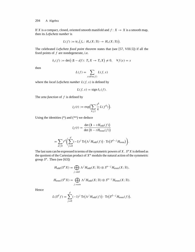
204 A Algebra
IfX is a compact, closed, oriented smooth manifold and f : X→ X is a smooth map,then its Lefschetz number is
L(f ) := trs(f∗ : H∗(X;R)→ H∗(X;R)
).
The celebrated Lefschetz fixed point theorem states that (see [57, VIII.5]) if all thefixed points of f are nondegenerate, i.e.
δx(f ) := det((1− df ) : TxX→ TxX
) �= 0, ∀f (x) = xthen
L(f ) =∑
x∈Fix(f )
L(f, x)
where the local Lefschetz number L(f, x) is defined by
L(f, x) = sign δx(f ).
The zeta function of f is defined by
ζf (t) := exp(∑k≥1
tk
kL(f k)
).
Using the identities (*) and (**) we deduce
ζf (t) = det(1− tHodd(f )
)det(1− tHeven(f )
)=∑d≥0
td( d∑j=0
(−1)j Tr(�jHodd(f )
) · Tr(Sd−jHeven
)).
The last sum can be expressed in terms of the symmetric powers ofX. SnX is defined asthe quotient of the Cartesian product ofXn modulo the natural action of the symmetricgroup Sn. Then (see [63])
Hodd(SnX) =
⊕j odd
�jHodd(X;R)⊗ Sn−jHeven(X;R),
Heven(SnX) =
⊕j even
�jHodd(X;R)⊗ Sn−jHeven(X;R).
Hence
L(Sdf ) =d∑j=0
(−1)j Tr(�jHodd(f )
) · Tr(Sd−jHeven(f )
),

§A.3 Extensions of Abelian groups 205
so thatζf (t) =
∑tdL(Sdf ).
If for example X is a Riemann surface of genus g, then H0(f ) = H2(f ) = 1. Ifwe denote by A ∈ Sp2g(Z) a symplectic matrix representing H1(f ) then we deduce
ζf (t) = det(1− tA)(1− t)2 .
§A.3 Extensions of Abelian groups
In this section we survey some basic facts concerning extensions of Abelian groupsneeded in surgery theory. We will denote by T the rational circle Q/Z and, for anyAbelian group A we will denote by A its dual
A := Hom(A,T).
SupposeA andC areAbelian groups. An extension ofA byC is a short exact sequenceof Abelian groups
0 → A→ B → C → 0.
Two extensions 0 → A→ Bi → C → 0, i = 0, 1 are isomorphic if there exists anisomorphism f : B0 → B1 such that the diagram below is commutative.
0 A B0 C 0
0 A B1 C 0.
�
�1A
�
�f
�
�1C
�
� � � �We denote by Ext(C,A) the set of isomorphism classes of extensions.
Proposition A.8 ([64]). (a)The correspondence Ext(C,−) is a covariant functor fromthe category of Abelian groups to the category of sets.
(b) The correspondence Ext(−, A) is a contravariant functor from Abelian groupsto sets.
Consider the group morphisms
∇A : A⊕ A→ A, a1 ⊕ a2 → a1 + a2
and�C : C → C ⊕ C, c → c ⊕ c.

206 A Algebra
Given two extensions Ei ∈ Ext(C,A)
Ei : 0 → A→ Bi → C → 0, i = 0, 1
we can construct in the obvious fashion E0 ⊕ E1 ∈ Ext(C ⊕ C,A ⊕ A). The Baersum of the two extensions is
E0 + E1 := ∇A∗ �∗C ∈ Ext(C,A)
where ∇A∗ �∗C is the composition
Ext(C ⊕ C,A⊕ A) �∗C−→ Ext(C,A⊕ A) ∇A∗−→ Ext(C,A).
Proposition A.9 ([64, 93]). The Baer sum introduces a structure of Abelian group onExt(C,A). The trivial (zero) extension is the split extension
0 → A→ A⊕ C → C → 0.
Moreover, for any short exact sequence of Abelian groups
0 → X→ Y → Z→ 0
and any Abelian group A we have the exact sequences
0 −→ Hom(Z,A) −→ Hom(Y,A) −→ Hom(X,A)δ−→ Ext(Z,A) −→ Ext(Y,A) −→ Ext(X,A) −→ 0
and
0 −→ Hom(A,X) −→ Hom(A, Y ) −→ Hom(A,Z)δ−→ Ext(A,X) −→ Ext(A, Y ) −→ Ext(A,Z) −→ 0.
Example A.10. Since Z is a projective Z-module we deduce that every extension
0 → C → B → Z→ 0
is split so that Ext(Z, C) = 0 for any Abelian group C. �
The next result is particularly relevant in topology.
Proposition A.11. Suppose C is a finite Abelian group. Given
λ : C → T := Q/Zwe define
Cλ = {q ∈ Q⊕ C; λ(c) = q modZ}.

§A.3 Extensions of Abelian groups 207
(a) The sequence Eλ defined by
0 → Zı→ Cλ
π→ C → 0
is exact, where ı is induced by the inclusions Z ↪→ Q⊕ 0 ↪→ Cλ while π is inducedby the natural projection Q⊕ C → C.
(b) The correspondence ψ : C := Hom(C,T)→ Ext(C,Z) defined by
C � λ → Eλ ∈ Ext(C,Z)
is a group isomorphism.
Proof. Part (a) is obvious. We will show that the correspondence in part (b) is abijection. For simplicity we will confine ourselves to the special case when C is acyclic group of order N .
Fix a generator t of C. Given an extension E ∈ Ext(C,Z)
0 → Z→ B → C → 0
we can find b0 ∈ B which maps to t . Then Nb0 maps to 0 ∈ C so that there existsm ∈ Z ↪→ B such that
Nb0 = m.(Abusing notations we can write b0 = m/N .) Now define
λE : C → T, kt → km/N mod Z.
The morphism λE does not depend on the choice of the generator t and the elementb0 ∈ B mapping to t . We have thus constructed a map
φ : Ext(C,Z)→ Hom(C,T), E → λE.
We let the reader check that
EλE = E ⇐⇒ ψ ◦ φ = 1,
andλEλ = λ ⇐⇒ φ ◦ ψ = 1. �
The result in the above proposition allows us to determine Ext(C, F ) where F isa free Abelian group of rank m. More precisely, we have a natural isomorphism
Ext(C, F )→ Hom(C, FQ/F )
where FQ := F ⊗Q. A morphism )λ : C → FQ/F ∼= F ⊗ T defines the extension
C)λ := {()q, c) ∈ (FQ)⊕ C; )λ(c) = )q modF }. (A.5)

208 A Algebra
Example A.12. Consider the inclusions ik : Z2 → Z2, k = 1, 2, given by the matrices
A1 :=[
4 00 1
], A2 :=
[2 00 2
].
These lead to the Abelian extensions
0 → Z2 A1−→ Z2 → Z4 → 0,
and0 → Z2 A2−→ Z2 → Z2 ⊕ Z2 → 0.
The first extension is given by the morphism
λ1 : Z4 → (T)2, 1 → (1/4, 0)
while the second is given by the morphism
λ2 : Z2 × Z2 → (T)2, (1, 0) → (1/2, 0), (0, 1) → (0, 1/2).
More generally, if G is a finite abelian group which admits a presentation
0 → FA−→ F → G→ 0
then this extension is classified by a morphism
G→ FQ/F.
This can be easily describes as follows. Consider the inverse
A−1 : FQ → FQ.
Observe that A−1(A(F )) = F ⊂ FQ so that we have an induced map
G ∼= F/(AF)→ FQ/F.
It is precisely the classifying map of the presentation. The mapG→ FQ/F is clearlyan inclusion. Conversely, every inclusion
G ↪→ FQ/F
produces a (class of) presentation(s) of G.It is perhaps instructive to see how this works in a concrete situation and to point
out a confusing fact. Suppose F ∼= Zn and A is described by an n× n matrix
Aej =∑i
aij ei, i, j = 1, . . . , n,

§A.3 Extensions of Abelian groups 209
where ei denotes the canonical integral basis of Zn. Suppose
A−1ej =∑i
a′ij ei , a′ij ∈ Q, i, j = 1, . . . , n.
Set G := Zn/AZn, and denote by [ei] the image of ei in G. Then the morphismG→ Tn corresponding to the extension
0 → ZnA−→ Zn→ G→ 0
is described by
[ej ] → a
′1j...
a′nj
mod Z.
The right-hand-side of the above equality is the j -th column of A−1.In topological applications the map G → Tn is described by n characters of G.
Since the dual G embeds in the dual ofZn it is customary to describe the map G→ Tn
as a vector consisting of n characters of Zn. In this case they are
)λ = (λ1, . . . , λn), λi([ej ]) = a′ij modZ, i, j = 1, . . . , n.
In other words, λi is the character of Zn described by the i-th row of A−1. �
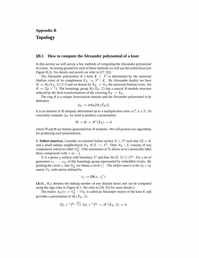
Appendix B
Topology
§B.1 How to compute the Alexander polynomial of a knot
In this section we will survey a few methods of computing the Alexander polynomialof a knot. As testing ground for each of these methods we will use the trefoil knot (seeFigure B.2). For details and proofs we refer to [27, 92].
The Alexander polynomial of a knot K ⊂ S3 is determined by the universalAbelian cover of its complement XK := S3 \ K . By Alexander duality we haveH := H1(XK,Z) ∼= Z and we denote by XK → XK the universal Abelian cover. SetR := Z[t, t−1]. The homology group H1(XK,Z) has a natural R-module structureinduced by the deck transformations of the covering XK → XK .
The ring R is a unique factorization domain and the Alexander polynomial is bydefinition
�K := ordR(H1(XK)
).
It is an element of R uniquely determined up to a multiplicative term ±tk , k ∈ Z. Toconcretely compute �K we need to produce a presentation
R→ G→ H 1(XK)→ 0
where R and G are finitely generated freeR-modules. We will present two algorithmsfor producing such presentations.
1. Seifert matrices.Consider an oriented Seifert surface � ⊂ S3 such that ∂� = Kand a small tubular neighborhood NK of � ↪→ S3. Then NK \ � consists of twocomponents which we label N±K . (The orientation of� allows us to canonically labelthese components with + or −.)� is a genus g surface with boundary S1 and thus H1(�,Z) ∼= Z2g . Fix a set of
generators x1, . . . , x2g of this homology group represented by embedded circles. Bypushing the circle xi intoN+K we obtain a circle x+i . The Seifert matrix is the 2g× 2gmatrix VK with entries defined by
vij := Lk(xi, x+j ).
Lk(K1,K2) denotes the linking number of two disjoint knots and can be computedusing the sign rules in Figure B.1. We refer to [59, 92] for more details.)
The matrix AK(t) := V TK − tVK is called an Alexander matrix of the knot K andprovides a presentation of H1(XK,Z)
Z[t, t−1]2g A(t)−→ Z[t, t−1]2g → H 1(XK,Z)→ 0.
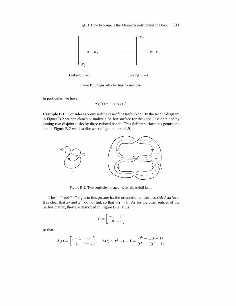
§B.1 How to compute the Alexander polynomial of a knot 211
K1K1
K2
K2
Linking = +1 Linking = −1
Figure B.1. Sign rules for linking numbers.
In particular, we have�K(t) ∼ detAK(t).
Example B.1. Consider as promised the case of the trefoil knot. In the second diagramin Figure B.2 we can clearly visualize a Seifert surface for the knot. It is obtained byjoining two disjoint disks by three twisted bands. This Seifert surface has genus oneand in Figure B.2 we describe a set of generators of H1.
x3
x2
x2 x1
x1
+ −
Figure B.2. Two equivalent diagrams for the trefoil knot.
The “+” and “−” signs in this picture fix the orientation of this two sided surface.It is clear that x2 and x+1 do not link so that v21 = 0. As for the other entries of theSeifert matrix, they are described in Figure B.3. Thus
V =[−1 1
0 −1
]so that
A(t) =[t − 1 −t
1 t − 1
], �(t) ∼ t2 − t + 1 = (t6 − 1)(t − 1)
(t2 − 1)(t3 − 1).
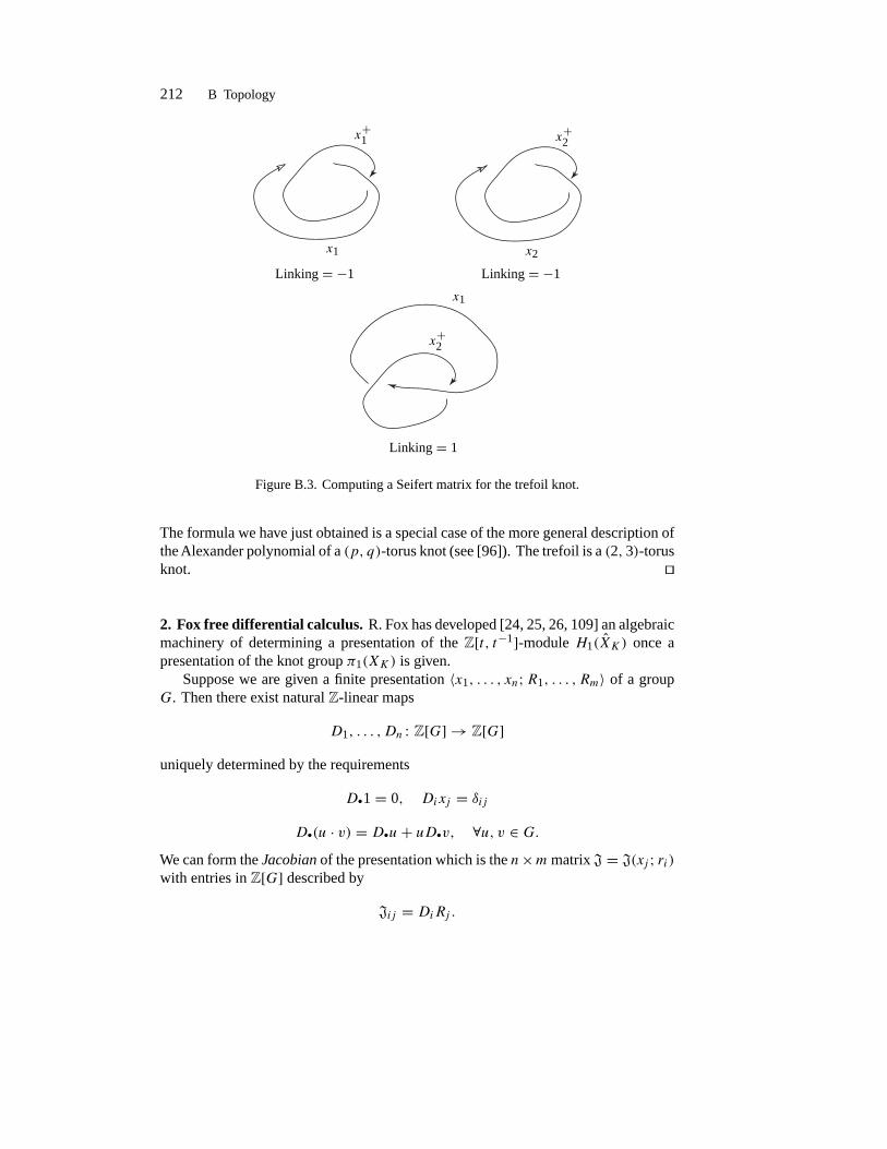
212 B Topology
x+1
x+2
x+2
x1
x1 x2
Linking = −1 Linking = −1
Linking = 1
Figure B.3. Computing a Seifert matrix for the trefoil knot.
The formula we have just obtained is a special case of the more general description ofthe Alexander polynomial of a (p, q)-torus knot (see [96]). The trefoil is a (2, 3)-torusknot. �
2. Fox free differential calculus.R. Fox has developed [24, 25, 26, 109] an algebraicmachinery of determining a presentation of the Z[t, t−1]-module H1(XK) once apresentation of the knot group π1(XK) is given.
Suppose we are given a finite presentation 〈x1, . . . , xn;R1, . . . , Rm〉 of a groupG. Then there exist natural Z-linear maps
D1, . . . , Dn : Z[G] → Z[G]uniquely determined by the requirements
D•1 = 0, Dixj = δijD•(u · v) = D•u+ uD•v, ∀u, v ∈ G.
We can form the Jacobian of the presentation which is the n×mmatrix J = J(xj ; ri)with entries in Z[G] described by
Jij = DiRj .

§B.1 How to compute the Alexander polynomial of a knot 213
If H denotes the abelianization of G, H := G/D(G), D(G) := [G,G] then weget a natural morphism ψ : Z[G] → Z[H ] and correspondingly, an n × m matrixJ := ψ(J) with entries in Z[H ]. The transpose of J defines a presentation theZ[H ]-module D(G)/D2(G)⊕ Z[H ],
Z[H ]m→ Z[H ]n→ D(G)/D2(G)⊕ Z[H ] → 0.
Suppose now that G is the fundamental group of the complement of a knot K ↪→ S3
G = GK := π1(XK), XK = S3 \K.If we are given a presentation of GK with n generators and m relations then
H = H1(XK) ∼= Z, D(G)/D2(G) ∼= H1(XK),
where as before, XK → XK denotes the universal Abelian cover. In this case we de-note by JK the abelianization of the Jacobian matrix J. Then theAlexander polynomialis the greatest common divisor of the set of (n− 1)× (n− 1)minors of J ; see [27] or[59, Chap.11] for more details. Equivalently, and more invariantly, we can define theAlexander polynomial as a generator of the first Fitting ideal F1(H1(XK)⊕Z[t, t−1])which admits a presentation given by the transpose of JK . Using Proposition 2.25 wededuce that F1(M) = F0(H1(XK)).
One can obtain a presentation of GK (called the Wirtinger presentation) from thediagram of K as follows.
•Orient the knot and mark the undercrossings in the order given by the orientation. Wehave thus divided K into n oriented arcs x1, . . . , xn each connecting two consecutiveundercrossings.• GK admits a presentation with x1, . . . , xn as generators and one relation for eachundercrossing, as described in Figure B.4. We can drop any one relation and still obtaina correct presentation. It is clear that all the generators of the Wirtinger presentationsare mapped by the abelianization map into the generator t of H1(XK) ∼= Z.
xixi
xjxj
xkxk
xj = xkxixk−1 xj = xk−1xixk
Figure B.4. Wirtinger relations.

214 B Topology
Example B.2. We consider again the trefoil knot. From the top of Figure B.2 we readthe following presentation
〈x1, x2, x3; x2 = x−13 x1x3, x3 = x−1
1 x2x1, x1 = x−12 x3x2〉.
Observe that only two generators are important since x3 = x−11 x2x1. We set a = x1
and b = x2 so that x3 = bab−1. We obtain the equivalent presentation
〈a, b; a = baba−1b−1, b = abab−1a−1〉 ⇐⇒ 〈a, b; bab = aba〉If we set
R = baba−1b−1a−1
then
DaR = Da(baba−1b−1)−(baba−1b−1)a−1 = Da(bab)−baba−1−baba−1b−1a−1
= Da(ba)− baba−1 − baba−1b−1a−1 = b − baba−1 − baba−1b−1a−1
DbR = Db(baba−1b−1) = Db(baba−1)− baba−1b−1 = Db(bab)− baba−1b−1
= Db(ba)+ ba − baba−1b−1 = 1+ ba − baba−1b−1.
By passing to abelianization we get
DaR = t − t2 − 1, DbR = 1+ t2 − tso that
JK = [−(t2 − t + 1) t2 − t + 1].This shows �K(t) ∼ t2 − t + 1. �
Remark B.3. The Fox free calculus works in the more general case of links withseveral components as well, with very few but obvious changes. The Wirtinger pre-sentation is obtained in the similar fashion, and we obtain a presentation of π1(XK)
with the same number ν of generators and relations. A generator g of this presentationwill represent in H1(XK) the same homology class as the meridian of the componentof the link to which g belongs. As in the case of knots, any relation can be droppedfrom the presentation. We obtain an exact sequence of Z[H ]-modules
Z[H ]ν J−→ Z[H ]ν → H1(XK)⊕ Z[H ]from which we deduce that
ordH1(XK) = F1(H1(XK)⊕ Z[H ]). �
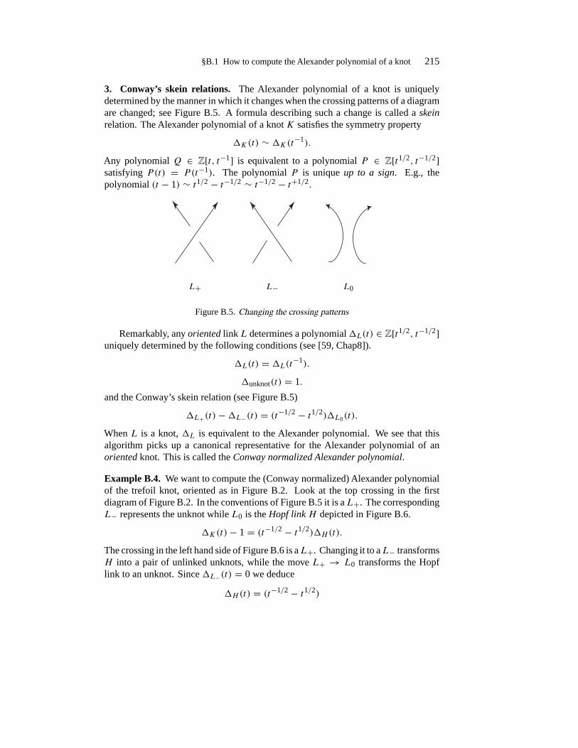
§B.1 How to compute the Alexander polynomial of a knot 215
3. Conway’s skein relations. The Alexander polynomial of a knot is uniquelydetermined by the manner in which it changes when the crossing patterns of a diagramare changed; see Figure B.5. A formula describing such a change is called a skeinrelation. The Alexander polynomial of a knot K satisfies the symmetry property
�K(t) ∼ �K(t−1).
Any polynomial Q ∈ Z[t, t−1] is equivalent to a polynomial P ∈ Z[t1/2, t−1/2]satisfying P(t) = P(t−1). The polynomial P is unique up to a sign. E.g., thepolynomial (t − 1) ∼ t1/2 − t−1/2 ∼ t−1/2 − t+1/2.
L+ L− L0
Figure B.5. Changing the crossing patterns
Remarkably, any oriented link L determines a polynomial�L(t) ∈ Z[t1/2, t−1/2]uniquely determined by the following conditions (see [59, Chap8]).
�L(t) = �L(t−1).
�unknot(t) = 1.
and the Conway’s skein relation (see Figure B.5)
�L+(t)−�L−(t) = (t−1/2 − t1/2)�L0(t).
When L is a knot, �L is equivalent to the Alexander polynomial. We see that thisalgorithm picks up a canonical representative for the Alexander polynomial of anoriented knot. This is called the Conway normalized Alexander polynomial.
Example B.4. We want to compute the (Conway normalized) Alexander polynomialof the trefoil knot, oriented as in Figure B.2. Look at the top crossing in the firstdiagram of Figure B.2. In the conventions of Figure B.5 it is aL+. The correspondingL− represents the unknot while L0 is the Hopf link H depicted in Figure B.6.
�K(t)− 1 = (t−1/2 − t1/2)�H (t).The crossing in the left hand side of Figure B.6 is aL+. Changing it to aL− transformsH into a pair of unlinked unknots, while the move L+ → L0 transforms the Hopflink to an unknot. Since �L−(t) = 0 we deduce
�H(t) = (t−1/2 − t1/2)

216 B Topology
Figure B.6. The Hopf link.
so that�K(t) = 1+ (t−1/2 − t−1/2)2 = t − 1+ t−1 ∼ t2 − t + 1. �
We want to explain a basic fact used in the proof of the Uniqueness Theorem 3.17.
§B.2 Dehn surgery and linking forms
The existing literature on Dehn surgery can be quite confusing, especially as far asthe various sign conventions are concerned. For the reader’s convenience, we havedecided to include several useful facts concerning this important concept, payingspecial attention to the many orientation conventions.
SupposeM3 is a rational homology 3-sphere, K ↪→ M3 is an oriented link inM3
with components K1, . . . ,Km, U = ⋃mj=1 Uj is a small open tubular neighborhoodof K and
MK := M \ U.Set T := ∂U and H∗(X) := H∗(X,Z) for any topological space X.
1. The homology ofMK as an extension ofH1(M). Since
H2(M) ∼= H 1(M) ∼= 0
we deduce from the long exact sequence of the pair (M,MK) that
0 → H2(M,MK)→ H1(MK)→ H1(M)→ H1(M,MK)→ 0.
Using excision we can rewrite
0 → H2(U , T )→ H1(MK)→ H1(M)→ H1(U , T )→ 0.
The long exact sequence of the pair (U , T ) now implies
H2(U , T ) ∼= ker(H1(T )→ H1(U)
) ∼= Zmand H1(U , T ) ∼= 0. Moreover ker
(H1(T ) → H1(U)
)admits a natural basis )µ =
(µ1, . . . , µm) consisting of meridians. More precisely, µj is the generator of
ker(H1(Tj )→ H1(Uj )
)

§B.2 Dehn surgery and linking forms 217
such thatLkM(µj ,Kj ) = 1
where LkM is theQ-valued linking number of two disjoint embedded circles. Denoteby Z〈 )µ〉 the free Abelian group generated by the meridians. We thus have a shortexact sequence
0 → Z〈 )µ〉 ∼= Zm j→ H1(MK)→ H1(M)→ 0,
wherej : H1(T )→ H1(MK)
is the inclusion induced morphism. As explained in Appendix §A.3, it defines anelement
)λK ∈ Ext(H1(M),Zm) ∼= Hom(H1(M),Tm).
We claim that
)λK(c) =m∑i=1
lkM(Ki , c)µi ∈ Q〈 )µ〉/Z〈 )µ〉, ∀c ∈ H1(M),
wherelkM : H1(M)×H1(M)→ T
is the linking form.To see this, denote by ν the order of H1(M). If c ∈ H1(M) is represented by an
embedded circle C ⊂ MK then
νC =∑j
kjµj ∈ H1(MK)
and thus
)λK(C) =∑ kj
νµj .
On the other hand
lkM(C,Ki ) = 1
ν
∑j
kj LkM(µj ,Ki ) = ki/ν mod Z.
Using the description (A.5) in §A.3 we deduce that
H1(MK) ∼={()α, c) ∈ Qm ×H1(M); αj = lkM(Kj , c) modZ, ∀j ∈ 1,m
}. (*)

218 B Topology
2. The morphismj : H1(T ) = H1(∂MK) → H1(MK). We use the exact sequenceof the pair (MK, T ) and we deduce
0 → H3(MK, T )→ H2(T )→ H2(MK)→ H2(MK, T )
→ H1(T )j→ H1(MK)→ H1(MK, T ) (**)
→ H0(T )→ H0(MK)→ 0.
To deal with the relative homology we use excision
H∗(MK, T ) ∼= H∗(M, U)and then the long exact sequence of the pair (M, U),
0 → H2(M, U)→ H1(U)→ H1(M)
→ H1(M,U)→ H0(U)→ H0(M)→ 0.
We deduce that
H2(MK, T ) ∼= ker(H1(U)→ H1(M)
) ∼= Zmand that the boundary map
H2(MK, T )→ H1(U)
is 1− 1. The above morphism factors through the inclusion induced map
ı : H1(T )→ H1(U)
so that the morphisms
H2(MK, T )→ H1(T ) and ker j ⊂ H1(T )ı→ H1(U)
must be 1− 1. Using the sequence (**) we deduce that H2(MK, T ) ∼= ker j so that
ı(ker j) ∼= ker(H1(U)→ H1(M)
). (B.1)
If we denote by 〈K〉 ⊂ H1(M) the subgroup generated by the components of the linkK we deduce that we have the short exact sequences
0 → ı(ker j)→ H1(U)→ 〈K〉 → 0
and
0 → H1(M)/〈K〉 → H1(M, U)→ Zm−1 ∼= ker(H0(U)→ H0(M))→ 0.
Hence,H1(MK, T ) ∼= H1(M)/〈K〉 ⊕ Zm−1,

§B.2 Dehn surgery and linking forms 219
andcoker j ∼= H1(M)/〈K〉. (B.2)
3. Longitudes. Suppose K is a link with a single component, i.e. a knot. IfM is notan integral homology sphere there is no canonical way of choosing an integral basisof H1(T )(∼= Z2). On the other hand, there is a natural way of choosing a Q-basis ofH1(T )⊗Q. A longitude is a generator λ of
ker j = ker(H1(T )→ H1(MK)
)such that µ ·λ > 0 where µ denotes a meridian and the intersection product is definedwith respect to the orientation of T as boundary of U . Denote by r the order of K inH1(M). From the identity (B.1) we deduce that λ = rK in H1(U). In particular, thisimplies µ · λ = r . Moreover, since λ bounds in the complement of K we deduce thatLkM(λ,K) = 0.
We can now conclude that any homology class c inH1(T ) is uniquely determinedby a pair (α, n) ∈ Q× Z satisfying the conditions
n := µ · c ⇐⇒ ı(c) = nK ∈ H1(U),
and
α := 1
r(c · λ)LkM(c,K) = n lkM(K,K) modZ.
As an element of H1(T ;Q) the cycle c has the decomposition
c = αµ+ nrλ.
Using the above basis ofH1(T ;Q)we can identify the inclusionH1(T ) ↪→ H1(T ;Q)with the inclusion G ↪→ Q2 where G is the additive subgroup of Q2 defined by theconditions
G ={ (α,n
r
)∈ Q⊕ 1
rZ; α = n lkM(K,K) modZ
}.
Observe that the longitude λ need not be a primitive element in H1(T ). Indeed,
1
mλ ∈ G ⇐⇒ n = r
m, n lkM(K,K) ∈ Z.
If we writelkM(K,K) = ν
r, 0 ≤ ν < r,
then the above conditions becomer
m,ν
m∈ Z,
so that we can choose m = (r, ν) (:=(g.c.d.(r, ν)). Hence
λ = (ν, r)λ0, λ0 ∈ H1(T ).

220 B Topology
Remark B.5. We would like to discuss a rather subtle point. The pair (r, ν mod rZ)was determined by the order and the self-linking number of K. We would like to showthat the same information is algebraically encoded by the pair of cyclesµ, λ ∈ H1(T ).
The Abelian group F := H1(T ) is free of rank two, and in order to performconcrete computations we need to choose Z-bases. This is involves non-canonicalchoices, and thus we need to be able to separate the invariant quantities from thosewhich are not. Clearly, the coordinates of µ and λ with respect to some Z-basis arenot invariant quantities. The determination of numerical invariants of the pair (µ, λ)boils down to a group theoretic problem.
Describe the space O of orbits of the group G := Aut(F ) acting diagonally onthe space P ⊂ F × F of pairs of linearly independent vectors.
Observe that π := (µ, λ) ∈ F × F , and the orbit{(T µ, T λ); T ∈ G
}corresponds to the different choices of bases of F . A pair π = (e1, e2) ∈ P definesan injection
jπ : Z2 → F, (n1, n2) → n1e1 + n2e2.
The extension
0 → Z2 jπ−→ F → Gπ := F/jπ(Z2)→ 0
is a complete invariant of the orbit (G ·π). It is completely characterized by the groupGπ , and the characteristic element
χ ∈ Hom(Gπ,T2) = Ext(Gπ,Z2).
In our special case, π = (µ, λ), Gπ is a cyclic group of order r , namely the cyclicgroup generated by the knot K ↪→ M . The last statement implicitly assumed theexistence of a canonical generator. This is indeed the case. Pick as generator theunique vector κ ∈ F ∩ {xµ+ yλ; x, y ∈ [0, 1]} such that µ · κ = 1. Geometrically,κ is the vertex of the Newton polygon of the cone sµ+ tλ, s, t > 0, closest to µ.
The characteristic element χ is given by the pair of characters χ1, χ2 ∈ Gπ .
χ1(K) = 1/r ∈ T, χ2(K) = lkM(K,K) = ν/r ∈ T.This can be seen easily using theZ-basis (µ, κ) ofH1(T ). In particular, λ = −νµ+rκ .
�
4. The morphism j : H1(T ) → H1(MK) revisited. Denote the components of K
by Kj , a small, open tubular neighborhood of Kj byUj , the meridian of Kj by µj andthe longitude of Kj by λj . Finally, denote by rj the order of Kj in H1(M).
Observe that if i �= j we have
�ji := ri LkM(Ki ,Kj ) = LkM(λi,Kj ) ∈ Z.

§B.2 Dehn surgery and linking forms 221
Since λi bounds inMKi we deduce we deduce that we have the following equality inH1(MK)
λi =∑j �=i�ji µj .
Using (*) in 1. on page 217 we deduce
H1(MK) ={(∑
j αjµj , c) ∈ Q〈 )µ〉 ×H1(M); αj = lkM(c,Kj ) mod Z, ∀j}.
Using the description of H1(T ) in 3., we deduce that the morphism j acts accordingto the rule
j : αjµj + niriλi →
(αjµj + ni
ri
∑s �=i�si µs, niKi
)=(αjµj + ni
∑s �=i
LkM(Ks ,Ki )µs, niKi), i, j = 1, . . . , m.
The natural map H1(MK)→ H1(M) is given by(∑j
αjµj , c)→ c.
5. Mayer–Vietoris interpretation. The Mayer–Vietoris sequence associated to thedecompositionM = U ∪MK leads to the Abelian group extension
0 → Z2m ∼= H1(T )ı⊕j−→ H1(U)⊕H1(MK)→ H1(M)→ 0. (B.3)
This extension is classified by a linear map
H1(M)→ H1(T )⊗ T.Arguing as in 1. we deduce that this classifying map is given by
c →∑j
lkM(Kj , c)µj ∈ H1(T )⊗ T.
6. Dehn surgery.The manifoldM can be described as a quotient space
U ∪f0 MK
where f0 : ∂U → ∂MK is an orientation reversing diffeomorphism. Given any orien-tation preserving diffeomorphism
)γ = (γ1, . . . , γm), γj : ∂Uj → ∂Uj
222 B Topology
we can form a new manifold
M )γ := U⋃f0◦ )γ
MK
called the Dehn surgery determined by )γ . Clearly the diffeomorphism type of M )γdepends only on the isotopy type of )γ . We denote by � the group of these isotopyclasses. Observe that
� ∼=m∏j=1
SL(H1(Tj )).
We denote by �0 the subgroup of � consisting of diffeomorphism which extend to U .It is not difficult to see thatM )γ depends only on the orbit )γ ◦ �0 ∈ �/�0.
The set of orbits �/�0 can be identified with the set of m-uples
)c := (c1, c2, . . . , cm) ∈m∏j=1
H1(Tj )
such that cj is a nontrivial primitive element of H1(Tj ). A diffeomorphism )γ belongsto the orbit labelled by )c if and only if
)γ ( )µ) = )c ⇐⇒ γj (µj ) = cj .For this reason, the Dehn surgery determined by )γ is often denoted byM)c.
Using the bases (µj , λj ) of H1(Tj ;Q) we can write
cj := αjµj + njrjλj , αj = nj lkM(Kj ,Kj ) mod Z. (***)
It is often convenient to identify cj with the pair of numbers (αj , nj ). These are knownas the surgery coefficients. WhenM is an integral homology sphere then the surgerycoefficients (α, n) are both integers. In this case the (α, n) surgery is traditionallyreferred to as the α/n-surgery. Furthermore, if n = 1 then the surgery is calledintegral. Two natural question arise.
A. Describe the homology ofM)c in terms of the homology ofM , invariants of the linkK ↪→ M and )c.B. Describe the linking form of H1(M)c) in similar terms.
7. The homology ofM�c. Arguing exactly as in 1., we obtain the extension
0 → Z〈 )µ〉 j◦γ−→ H1(MK)→ H1(M)c)→ 0
or, equivalently,
0 → Z〈)c〉 j−→ H1(MK)→ H1(M)c)→ 0.

§B.2 Dehn surgery and linking forms 223
Using the description of j in 4. we deduce that H1(M)c) is the quotient of H1(MK)
modulo the subgroup generated by(αiµi + ni
∑j �=i
LkM(Kj ,Ki )µj , niKi).
If we form the m×m matrix P(K, )c) with rational entries
pji ={ni LkM(Kj ,Ki ) j �= iαi j = i,
we deduce thatM)c is a rational homology sphere if and only if
det P(K, )c) �= 0.
We consider two extreme situations.
a. M is an integral homology sphere.Then P = P(K, )c) defines a presentation ofH1(M)c),
0 → ZmP−→ Zm→ H1(M)c)→ 0.
Alternatively,M)c can be given the Mayer–Vietoris description
0 → H1(T )i⊕j◦γ−−−−→ H1(U)⊕H1(MK)→ H1(M)c)→ 0.
b. K is consists of a single component,m = 1. Set α := α1, n := n1 etc. α and nare constrained by
α ≡ n lkM(K,K) mod Z.
Then
H1(Mc) = H1(MK)/Z〈c〉∼= {(tµ, γ ) ∈ Q〈µ〉 ×H1(M); t = lkM(γ,K) modZ}/Z〈αµ+ nK〉.
8. Linking theory on H1(M�c). We will again consider two cases.
a. The manifold M is an integral homology sphere.In this case H1(M)c) admits apresentation of the form
0 → Z〈 )µ〉 P(K,)c)−−−−→ Z〈 )µ〉 → H1(M)c)→ 0.
According to the computations in Example A.12, this extension is classified by themap
$ := P(K, )c)−1 : Z〈 )µ〉/PZ〈 )µ〉 → Q〈 )µ〉/Z〈 )µ〉.On the other hand, according to the computation in 1., page 216, this classifying mapcan be described in terms of the linking theory on H1(M)c). We denote by [Kj ])c the
224 B Topology
homology class of the core of Uj in H1(M)c). These classes define via the linkingform ofM)c a vector of n characters of H1(M)c) which classifies the above extension.Moreover, we have
lkM)c ([Ki])c, [µj ]) = $ij mod Z, ∀i, j, (B.4)
where $ := ($ij ) = P−1, that is
P−1µj =∑i
$ijµi.
If we denote by (•, •) the natural inner product on Q〈µ〉 defined by (µi, µj ) = δij ,then we can write
$ij = (µi, P−1µj ).
If we are “lucky enough”, so that [Kj ])c generateH1(M)c), then the above trick allowsus to determine the linking form ofM)c. In fact, this is not a matter of luck.
Proposition B.6. Suppose that the surgery coefficient of Ki is piqi
so that
P(K, )c) = (pij )1≤i,j≤nwhere
pij ={qj LkM(Ki ,Kj ) if i �= jpi if i = j.
Then the classes µi generate H1(M)c), and we have the equalities
qi[Ki])c = −µi in H1(M)c), ∀i.Moreover,
lkM)c (µi, µj ) = −qi(µi, P−1µj ) mod Z.
Proof. The Dehn surgery is described by a family
)γ = (γ1, . . . , γm) ∈m∏j=1
SL(2,Z), γj :=[pj αjqj βj
], pjβj − αjqj = 1.
These matrices describe the attaching rules
mi → j(ci) = j(piµi + qiλi) = bi := piµi + qi∑j �=i�jiµj ,
li → j(αiµi + βiλi) = ki := αiµi + βi∑j �=i�ijµj ,

§B.2 Dehn surgery and linking forms 225
where mi (resp. li) denotes the meridian (resp. the longitude) of the i-th attachingsolid torus and
�ij = LkM(Ki ,Kj ) ∈ Z.The group H1(M)c) is the quotient of Z〈 )µ〉 modulo the lattice spanned by the vectorsbi . Using the identities
pjβj − αjqj = 1
we deduceβibi − qiki = µi
which shows that −qi[Ki])c = [µi] in H1(M)c). The second statement in the proposi-tion follows from the identity
−qi$ij = −qi lkM)c ([Ki], [µj ]) = lkM)c ([µi], [µj ]) mod Z. �
Remark B.7. Denote by P0 the symmetric matrix defined by
pij ={�ij if i �= jpiqi
if i = j.
Then P(K, )c) = P0 ·diag(q1, . . . , qn), and the (i, j)-th entry of the symmetric matrixP−1 is qi$ij , that is
(µi, P−10 µj ) = −qi(µi, P−1µj ).
The linking form ofM)c is completely characterized by P−10 via the equalities,
lkM(µi, µj ) = −(µi, P−10 µj ). �
Example B.8. The arguments in the proof of the above proposition can be easilygrasped in the following simple situation. Suppose K is a knot in M := S3. TheDehn surgeries on K are determined by a pair of relatively prime positive integers(p, q). If K is the unknot in S3 then the (p, q) surgery on K produces the lens spaceL(p,−q). Denote by λ and µ the longitude and respectively the meridian of K suchthat µ · λ = 1. The complementMK is a solid torus and µ is its core. µ is a generatorof H1(MK). The characteristic curve of the (p, q) surgery is pµ+ qλ.
The first homology group of the manifoldMp/q := Mc admits the presentation
0 → Zµp·−→ Z )µ ∼= H1(MK)→ H1(Mp/q)→ 0.
We deduce that H1(Mp,q) and the generator µ of H1(MK) induces a generator ofH1(Mp/q). Moreover, according to Example A.12 the above extension is classifiedby the map
Zp → T, 1 mod pZ → 1/p modZ.
226 B Topology
If we now denote by [•]p/q the class in H1(Mp/q) determined by a closed curve • wededuce
lkMp/q ([K]p/q, [µ]p/q) = 1/p.
Since [µ]p/q is a generator of H1(Mp/q) we can write
[K]p/q = x[µ]p/q, x ∈ Z mod pZ.
Now observe that the gluing map γ of this Dehn surgery is described by a matrix
γ :=[p α
q β
]∈ SL(2,Z)
with inverse
γ−1 =[β −α−q p
].
The meaning of the entries of this matrix are given by the attaching rules
µ → c = pµ+ qλ ∈ H1(∂MK), K = λ → αµ+ βλ ∈ H1(∂MK).
Since λ = 0 ∈ H1(MK) deduce from these rules that
[K]p/q = α[µ]p/q .Since det γ = pβ − αq = 1 we deduce α = −q−1 mod pZ. Hence
lkMp/q (−q−1[µ]p,q, [µ]p,q) = 1/p,
so thatlkMp/q ([µ]p/q, [µ]p/q) = −q/p mod Z. �
b. K has only one component butM may have nontrivial homology. In this case itis wiser to treatM andMc “democratically”, as equal partners. These two manifoldshave something in common, the 3-manifold with boundary MK. This notation doesnot respect our “democracy rule” and we will setN := MK. The Dehn surgery processcan now be described as attaching the solid torus
U := S1 ×D2
to the boundary ∂N so that the curve pt × ∂D2 is attached along a primitive curveµ ∈ H1(∂N). We denote the resulting closed manifold by Nµ. (In the old notationsM = Nµ.)
As an aside, note that the homologies of N and ∂N contain no information aboutthe homology sphereM . This is determined by an additional internal data, namely thehomology class inH1(T ) carried by the meridian of the knot. We can loosely rephrase
§B.2 Dehn surgery and linking forms 227
this by saying that the homology groups of N have no idea about the manifold M .There is however one element in H1(T ) which carries this information.
As the complement of a knot in a rational homology sphere, the manifold N hasseveral special topological features we would like to single out and rephrase in alanguage which makes no mention ofM .
Observe first that b1(N) = 1. Moreover, the boundary map
H2(N, ∂N)→ H1(∂N)
is injective (see 2., page 218). Its image is a rank one subgroup of H1(∂N) generatedby the longitude λ. This subgroup is isomorphic to the kernel of the morphism
j : H1(∂N)→ H1(N).
λ need not be a primitive element of H1(∂N) and we can write
λ = m0λ0, m0 > 0, λ0 ∈ H1(∂N) is primitive.
At 2. we have shown that H1(N, ∂N) is a torsion group. Using the Universal Coeffi-cients Theorem we obtain the split exact sequence
0 → Ext(H1(N, ∂N),Z)→ H 2(N, ∂N)→ Hom(H2(N, ∂N),Z)→ 0.
The Poincaré duality now leads to the isomorphisms
H1(N) ∼= H 2(N, ∂N) ∼= Hom(H2(N, ∂N),Z)⊕ Ext(H1(N, ∂N),Z)∼= Hom(H2(N, ∂N),Z)⊕ Hom(H1(N, ∂N),T).
This isomorphism is most conveniently expressed in intersection theoretic terms. De-note by Hτ1 (N) the torsion part of H1(N). The above isomorphisms implies that wehave a nondegenerate linking pairing
lkN : Hτ1 (N)×H1(N, ∂N)→ T.
We obtain a bilinear map
lkN : Hτ1 (N)×Hτ1 (N)→ T, lkN(c1, c2) = lkN(c1, i(c2))
where i denotes the morphism H1(N) → H1(N, ∂N). This is a symmetric, yetpossibly degenerate form. If we identify H2(N, ∂N) with ker j = Z〈λ〉 ⊂ H1(∂N)
we see that we have a map
L : H1(N)→ Hom(Z〈λ〉,Z) ∼= Z ⇐⇒ Lk : H1(N)× Z〈λ〉 → Z
which can be described geometrically as the linking with λ. λ bounds a chain� in Nand we define
L(c) = LkN(c, λ) := #(c ∩�), ∀c ∈ H1(N).

228 B Topology
Observe thatL(jz) = λ · z, ∀z ∈ H1(∂N),
where the dot denotes the (skew-symmetric) intersection pairing on H1(∂N) definedusing the orientation on ∂N as boundary of N . The subgroup jH1(∂N) ⊂ H1(N) ismapped by L onto the subgroup m0Z ⊂ Z. We obtain a short exact sequence
0 → Hτ1 (N) = kerL→ H1(N)L−→ Z→ 0.
Any σ0 ∈ H1(N) such that Lk(σ0, λ) = 1 produces a splitting of the above sequence
H1(N) ∼= Hτ1 (N)⊕ Z〈σ0〉.Moreover, any element c ∈ H1(N) determines a morphism
c� = lkN(c,−) ∈ H1(N, ∂N).
The element c is completely determined by the quantities
c� ∈ H1(N, ∂N), n(c) := LkN(c, λ) ∈ Z.More precisely, we can write c = [c] + cτ
[c] = n(c)σ0, cτ := c − [c].Define c∗ ∈ Hom
(H2(N, ∂N),Z
)⊕ Hom(H1(N, ∂N),T)
c∗ = [c]∗ + c�, [c]∗ := LkN(c,−), c� = lkN(cτ ,−).The correspondence c←→ c∗ is precisely the Poincaré duality.
Before we continue this line of thought we want to present a guiding examplewhich will provide some intuition behind the above abstract constructions.
Example B.9. Suppose N is the complement of a knot K in a rational homologysphere M . Denote by r the order of K in H1(M). (If H1(M) = 0 we set r = 1.)Since the linking form onM is nondegenerate there exists a knot K� ⊂ M such that
LkM(K,K�) = 1
r.
ThenH1(N) ∼= {(α, c) ∈ Q×H1(M); α = lkM(c,K) mod Z}.
The pair (1/r,K�), which corresponds to the homology class inN carried by the knotK�, can be taken as a generator of the free part of H1(N). We will denote this classsimply by K�. Observe that it corresponds to the choice σ0 ∈ H1(N) explained in thepreceding discussion. The torsion part of H1(N) is isomorphic to{(0, c) ∈ Q×H1(M); lkM(K, c) = 0
} ∼= K⊥ := ker lkM(K,−) : H1(M)→ Zr .

§B.2 Dehn surgery and linking forms 229
We have seen in 2., page 218, that
H1(N, ∂N) ∼= H1(M)/〈K〉.The linking form onM induces a nondegenerate pairing
ker lkM(K,−)×H1(M)/〈K〉 → T.
This is precisely the nondegenerate linking
lkN : H1(N)τ ×H1(N, ∂N)→ T.
The curve λ ∈ H1(∂N) which generates ker j can be uniquely written asm0λ0 whereλ0 is primitive. If we set
ν
r= lkM(K,K)
then m0 = (ν, r). Thus m0 can be determined from λ and r using the equality
λ · µ = r,where ∂N is oriented as boundary of N . We can describe
H1(∂N) � z = αµ⊕ nrλ, α = n lkM(K,K).
The morphism j has the form
αµ+ nr→ (α, nK) ∈ H1(N).
Suppose we have chosen ω0 ∈ H1(N) such that λ0 · ω0 = 1. There is no uniquechoice but each such choice can be represented as
ω0 = a0µ+ n0
rλ, a0 − n0ν
r∈ Z.
The equation λ0 · ω0 = 1 implies
ra0 = m0
so thatm0
r= n0ν
rmod Z.
If we writeν = m0ν0, r = m0r0, (ν0, r0) = 1
we deduce1
r0= n0ν0
r0mod Z

230 B Topology
so that
n0ν0 = 1 mod r0Z, a0 = 1
r0
and
jω0 =(
1
m0µ, n0K
), jλ0 = (0, r0K). �
We can finally explain what do we need to know to compute how the linking formof a rational homology sphere changes by performing a Dehn surgery along a knot.
Suppose N is the complement of a knot K in a rational homology spheres N1.µ ∈ H1(∂N) is a primitive curve such that
r := λ · µ > 0.
Fix κ ∈ ∂N such that κ · µ = 1. We can assume that Dehn surgery is given by theidentification
S1 × ∂D2 → ∂N,
S1 × pt → κ, pt × ∂D2 → µ.
If O denotes the center of D2, we denote by K the image of S1 ×O in Nµ. At 1. wehave shown that we have an extension
0 → Z〈µ〉 → H1(N)→ H1(Nµ)→ 0
classified by the morphism
lkNµ(K,−) : H1(Nµ)→ T.
We have the following result.
Proposition B.10. The linking form of Nµ is completely determined by the followingdata.
I 1. µ, κ ∈ H1(∂N) such that κ · µ = 1.
I 2.The Abelian groupsH1(N),H1(N, ∂N) and the morphism j : H1(∂N)→ H1(N).Fix a generator λ of ker j and set r = λ ·µ, k = λ · κ . Fix� ∈ H2(N, ∂N) such that∂� = λ and denote bym0 the positive integer such thatλ = m0λ0 whereλ0 ∈ H1(∂N)
is a primitive class.
I 3. The Poincaré duality linking pairing
lkN : Hτ1 (N)×H1(N, ∂N)→ T.
I 4. A cycle σ0 ∈ H1(N) such that σ0 · � = 1. Algebraically, this is equivalent tochoosing a splitting
H1(N) = free part⊕ torsion part.

§B.2 Dehn surgery and linking forms 231
I 5. A positive integer r0 and a cycle
ν = αµ+ nrλ ∈ H1(∂N)
such thatr0σ0 − jν = 0 ∈ H1(N).
Remark B.11. The preceding discussion and Example B.9 show that these data arecompletely determined by the homological properties of the pair (N1,K). In otherwords, the computation of the linking form of a rational homology sphere can bedetermined by performing only homological computations. This is certainly not thecase for the Reidemeister torsion which is not a homotopy invariant. �
Proof. Using I 1 and I 2 we can now determine
H1(Nµ) := H1(N)/〈jµ〉and thus the canonical extension
0 → Z〈µ〉 → H1(N)proj−−−→ H1(N)/〈jµ〉 ∼= H1(Nµ)→ 0.
The element K ∈ H1(Nµ) is the image of jκ in H1(N)/〈jµ〉. The above extensioncompletely determines the morphism
lkNµ(K,−) : H1(Nµ)→ T.
Observe that Hτ1 (N) embeds in H1(Nµ) = H1(N)/〈jµ〉 as the kernel Kµ of thismorphism. We can now produce an isomorphism
H1(Nµ)/〈K〉 → H1(N, ∂N) = H1(N)/Range j
by going up-and-down along the diagram below (with exact diagonals)
Range j Z〈µ〉
H1(N)
H1(Nµ) H1(N, ∂N)
H1(Nµ)/〈K〉
��� �
proj ����
.
Using I 3 we now obtain the nondegenerate pairing
lkNµ : Kµ ×H1(Nµ)/〈K〉 → T.
232 B Topology
In particular, this implies we can now compute all the pairings of the form lkNµ(u, v)where u, v ∈ H1(Nµ) and at least one of them is in Kµ.
To complete the determination of lkNµ we will need to use the following elementaryresults.
Lemma B.12. Suppose K� ∈ H1(Nµ) is such that
lkNµ(K,K�) = 1/r ∈ T.
Then for all u, v ∈ H1(Nµ) we have
lkNµ(K, u) =n(u)
r, lkNµ(K, v) =
n(v)
r, 0 ≤ n(u), n(v) < r
u0 := u− n(u)K�, v0 := v − n(v)K� ∈Kµ
and
lkNµ(u, v) = lkNµ(u0 + n(u)K�, v0 + n(v)K�
)= lkNµ(u0, v0)+ lkNµ
(n(v)u0 + n(u)v0,K
�)+n(u)n(v) lkNµ(K
�,K�).
The above result shows that in order to determine lkNµ we need to find the self-linking number lkNµ(K
�,K�) for some solution K� of the equation
lkNµ(K,K�) = 1/r ∈ T.
The cycle σ0 ∈ H1(N) described in I 4 descends to a solution [σ0] ∈ H1(N)/Z〈µ〉 ∼=H1(Nµ) of above equation. We can now represent the cycle ν of I 5 as a linear com-bination
ν = αµ+ nr�
so thatrr0σ0 = rjν = rαµ+ nλ = nλ = n∂�.
ThuslkNµ(σ0, σ0) = n
rr0(σ0 ∩�) = n
rr0. �
The proof of the above proposition explicitly describes an algorithm for computingthe change in the linking form under a Dehn surgery. As our next example will show,the concrete implementations of this algorithm can be computationally demanding.
Example B.13(Surgery onM := L(24, 23)). Fix a generator g0 of H1(L(24, 1)) ∼=Z24 such that the linking form q has the description
q(xg0, yg0) = −xy
24∈ T.
§B.2 Dehn surgery and linking forms 233
Fix a knot K0 in this lens space representing 4g0 in homology. Denote U0 a small(open) tubular neighborhood of K0inM , and by µ0 its meridian oriented such that
λ0 · µ0 = 6,
where the above intersection pairing uses the orientation on ∂U0 as boundary ofN := M \ U0. Thus ord (K) = 6 and
q(K0,K0) = −16
24= −4
6= −2
3∈ T.
The kernel of j : H1(∂N)→ H1(N) is generated by a curve λ ∈ H1(∂N). Accordingto Remark B.5 we can choose a basis of H1(T ) so that µ0 has the coordinates (0, 1)while λ has the coordinates (6, 4). Then
H1(N) ∼={(αµ0, cg0) ∈ Q〈µ0〉 × Z24〈g0〉; α = −
c
6modZ
}.
ThusHτ1 (N) = ker lkM(K0,−) ∼= 6Z24 ∼= Z4〈u0 := 6g0〉.
SimilarlyH1(N, ∂N) ∼= H1(M)/〈K0〉 ∼= Z4〈v0〉,
where v0 denotes the generator defined as the image of g0 in H1(M)/〈K0〉. Then
lkN(u0, v0) = lkM(6g0,g0) = −1
4.
This equality produces I 3. Observe that
lkM(−g0,K0
) = 1
6.
Thus σ0 := (1/6µ0,−g0) ∈ H1(N) solves I 4.A nontrivial Dehn surgery on K0 is described by a primitive curve µ ∈ H1(∂N)
such that µ �= µ0. Suppose µ = (1, 0) := − 23µ+ 1
6λ, i.e. we perform a (−2/3, 1)-surgery. Then we can choose κ := (0, 1) = µ0. Observe that
jµ =(− 2
3µ0,K0 = 4g0
)∈ H1(N), j(κ) = (1, 0) ∈ H1(N).
Hence H1(Nµ) is defined by the extension
0 →{(− 2n
3, 4ng0
); n ∈ Z
}↪→ {(α, cg0); α +
c
6∈ Z}→ H1(Nµ)→ 0.
More explicitly, observe that we have the direct sum decomposition
H1(N) = Z〈σ0〉 ⊕ Z4〈u0 := 6g0〉,
234 B Topology
and we can write jµ = −4σ0. We conclude that
H1(Nµ) ∼= Z4〈σ0〉 ⊕ Z4〈u0〉.The extension
0 → Z(·4σ0,0)−−−−−→ Z⊕ Z4 → Z4σ0 ⊕ Z4u0 → 0
is classified by the character
χ : Z4σ0 × Z4u0 → T, χ(σ0) = 1
4, χ(u0) = 0.
The cycle jκ = 6σ0 ⊕ u0 ∈ H1(N) projects to the cycle
K = 2σ0 ⊕ u0 ∈ H1(Nµ),
and we have
lkNµ(K, σ0) = χ(σ0) = 1/4, lkNµ(K,u0) = χ(u0) = 0.
We deduce thatker lkNµ(K,−) ∼= Z4〈u0〉.
Now observe that σ0 ∈ H1(N) descends to a generator ofH1(Nµ)/〈K〉 ∼= Z4. It musttherefore descend to a generator of
H1(N, ∂N) ∼= H1(N)/Range j .
We have identified H1(N, ∂N) ∼= H1(M)/〈K0〉 with the cyclic group of order 4 withgenerator v0 induced by g0 ∈ H1(M). Observe that g0 lifts to −σ0 ∈ H1(N). Thusthe isomorphism
Z4〈σ0〉 ∼= H1(Nµ)/〈K〉 ∼= H1(N, ∂N) ∼= Z4〈v0〉can be concretely described by the correspondence σ0 → −v0. We conclude that thepairing
lkNµ : ker lkNµ(K,−)×H1(Nµ)/〈K〉 → T
has the formlkNµ(xu0, yσ0) = − lkN(xu0, yv0) = xy
4.
Hence the pairing
lkNµ : ker lkNµ(K,−)×H1(Nµ)→ T
is given by
lkNµ(u0, σ0) = 1
4, lkNµ(u0,u0) = lkNµ(u0,K− 2σ0) = −1
2.
Since 4σ0 = −jµ we deduce that lkNµ(σ0, σ0) = 0. Summarizing all of the abovewe deduce
lkNµ(au0 + bσ0, xu0 + yσ0) = ay + bx4
+ ax2. �
§B.2 Dehn surgery and linking forms 235
So far we have discussed only Dehn surgeries which produce rational homologyspheres. We want to spend the rest of this section discussing the remaining case.
Suppose N is homeomorphic to the complement of a tubular neighborhood ofa knot in a rational homology sphere M . Set T := ∂N . Orient T as boundary ofN . Denote by λ ∈ H1(T ) a longitude, i.e a generator1 of the kernel of the inclusioninduced map H1(T ) → H1(N). Denote by m0 the divisibility of λ, i.e. m0 is thepositive integer such that λ = m0λ0 where λ0 is a primitive element of H1(T ).
For any primitive class c ∈ H1(T ) denote byNc the closed three-manifold obtainedfrom N by Dehn surgery with data c. If λ · c �= 0 the three-manifold Nc is a rationalhomology sphere. When c = λ0 the three-manifold Nλ0 is a rational homologyS1 × S2. We denote it by N0. We want to describe the homological invariants of N0in terms of the homological invariants of N . Denote by U the solid torus we attach toN to produce N0. Note that
H3(N0) ∼= H3(N0, N) = Z, 0 = H1(U , T ) ∼= H1(N0, N)
andH2(N) = 0, H2(N0, N) ∼= H2(U , T ) ∼= Z.
As generator of H2(U , T ) we can take the disk Dµ spanning the meridian. The longexact sequence of the pair (N0, N) now implies
0 → H2(N0)→ H2(U , T )(∼= Z)→ H1(N)→ H1(N0)→ 0.
Since the generator Dµ of H2(U , T ) goes to the torsion class j(λ0) ∈ H1(N) wededuce that the image of H2(N0) in H2(N0, N) is generated by m0[Dµ]. Moreover,we have a short exact sequence
0 → 〈jλ0〉 → H1(N)→ H1(N0)→ 0. (B.5)
where 〈jλ0〉 denotes the cyclic group of order m0 generated by jλ0.Consider now the long exact sequence of the pair (N0, U ). Denote by � ∈
H2(N, ∂N) a relative 2-cycle bounding λ. Observe that H2(N, ∂N) ∼= H2(N0, U ) isgenerated by �. Since H2(U) = 0 we deduce
0 → H2(N0)→ H2(N, ∂N) ∼= Z〈�〉 ∂→ H1(U)→ H1(N0)→ H1(N, ∂N)→ 0.
The connecting morphism ∂ is trivial because ∂� = λ = m0µ→ 0 ∈ H1(U) so thatwe obtain an isomorphism
H2(N0) ∼= H2(N, ∂N) ∼= Z〈�〉,and a short exact sequence
0 → H1(U)→ H1(N0)→ H1(N, ∂N) ∼= coker j → 0. (B.6)
1There are two generators, and a choice can be determined by fixing an orientation.

236 B Topology
We denote by K0 the homology class in H1(N0) carried by the core of U and by iKthe inclusion induced morphism iK : H1(U)→ H1(N0). Hence
H1(N, ∂N) ∼= H1(N0)/〈K0〉.The extension (B.6) defines a character of H1(N, ∂N) which, in view of the Poincaréduality on (N, ∂N), can be identified with the linking by a torsion element inH1(N).Using (B.5) we deduce that this is given by the linking with λ0. Note also that K isnot a primitive class. It has divisibility m0.
Dualizing the sequence (B.6) we deduce
1 → H1(N, ∂N)→ H1(N0)ˆiK−→ H1(U)→ 1
Restricting the second map to the identity component of H1(N0)we obtain a surjection
S1 ∼= H1(N0)id
ˆiK� H1(U)id∼= S1.
Since the linking number of j(K0) and � (in N ) is m0 we deduce that the map i�K is
an m0-cover. Denote by z the coordinate on H1(U), and by T the coordinate on theidentity component of H1(N0). The above map is described by z = T m0 .
Dualizing the sequence (B.5) we obtain the short exact sequence
1 → H1(N0)→ H1(N)→ Um0 → 1, (B.7)
whereUm0 is the group ofm0-th roots of 1. Restricting to the identity components wededuce
H1(N0)id = H1(N)id .
Denote by TX the Fourier transform of the Reidemeister torsion of X. The surgeryformulæ have the form
TN0 · ˆiKTU = TN |H1(N0). (B.8)
Observe now that sinceH is an Abelian group of positive rank the augmentation map
aug : Map(H,C)→ Map(H/Tors(H),C)
is precisely the integration along the fibers of H → H/Tors(H). If f is the Fouriertransform of f ∈ Map (H,C) then the Fourier transform of aug(f ) is the restrictionof f to the identity component of H .
If we now further restrict the surgery formula (B.8) to the identity component ofH1(N0) and then take the inverse Fourier transform we deduce
TaugN0(T )(1− T m0)−1 ≈ T
augN (T ).

§B.2 Dehn surgery and linking forms 237
Recalling thatT
augN (T ) ∼ �N(T )(1− T )−1,
where �N(T ) denotes the Alexander polynomial of N , we conclude
TaugN0(T ) ∼ �N(T )
(1− T )(1− T m0).

Bibliography
[1] M.F. Atiyah, R. Bott: A Lefschetz fixed point formula for elliptic complexes II. Applica-tions, Ann. of Math. 88 (1968), 451–491.
[2] M.F. Atiyah, V.K. Patodi, I.M. Singer: Spectral asymmetry and Riemannian geometry I,Math. Proc. Cambridge Philos. Soc. 77 (1975), 43–69.
[3] S. Baldridge: Seiberg-Witten invariants of 4-manifolds with free circle actions,math.GT/9911051.
[4] J.M. Bismut, W. Zhang: An extension of a theorem by Cheeger and Müller, Astérisque205, 1992.
[5] G.E. Bredon: Topology and Geometry, Grad. Texts in Math. 139, Springer-Verlag, 1993.
[6] G.E. Bredon: Sheaf Theory, Grad. Texts in Math. 170, Springer-Verlag, 1997.
[7] G.W. Brumfiel, J. W. Morgan: Quadratic functions, the index modulo 8, and a Z/4-Hirzebruch formula, Topology 12 (1973), 105–122.
[8] G. Burde, H. Zieschang: Knots, de Gruyter Stud. Math. 5, Walter de Gruyter, 2003.
[9] D. Burghelea, L.Friedlander, T. Kappeler: Witten deformation of the analytic torsionand the Reidemeister torsion, Voronezh Winter Mathematical Schools, Amer. Math. Soc.Transl. Ser. (2) 184, Amer. Math. Soc., Providence, RI, 1998, 23–39; also available athttp://www.math.ohio-state.edu/ burghele/.
[10] D. Burghelea, L.Friedlander, T. Kappeler, P. MacDonald: Analytic and Reidemeistertorsion for representations in finite type Hilbert modules, Geom. Funct. Anal. 6 (1996),751–859.
[11] A. Carey, M. Marcolli, B.L. Wang: Exact triangles in Seiberg-Witten-Floer homology.Part I: the geometric triangle, math.DG/9907065, Comm. Contemp. Math., to appear.
[12] A. Cayley: On the theory of elimination, Cambridge and Dublin Math. J. 3 (1848),116–120; Collected Papers Vol.1, Cambridge University Press, 1889, 370–374.
[13] T.A. Chapman: Topological invariance of Whitehead torsion, Amer. J. Math. 96 (1974),488–497.
[14] J. Cheeger: Analytic torsion and the heat equation, Ann. of Math. 109(1979), 259–322.
[15] W.Chen: Casson invariant and Seiberg-Witten gauge theory, Turkish J. Math. 21 (1997),61–81.
[16] M.M. Cohen: A course in simple homotopy theory, Grad. Texts in Math. 10, Springer-Verlag, 1973.
[17] J.F. Davis, P. Kirk: Lecture Notes in Algebraic Topology, Grad. Stud. in Math., Amer.Math. Soc., 2001
[18] P. Deligne: Le déterminant de la cohomologie, in Current Trends in Aritmetical AlgebraicGeometry, Contemp. Math. 67, Amer. Math. Soc, 1987, 93–177.
[19] G. DeRham, S. Maumary, M.A. Kervaire: Torsion et Type Simple d’Homotopie, LectureNotes in Math. 48, Springer-Verlag, 1967.
240 Bibliography
[20] A. Dimca: Singularities and the Topology of Hypersurfaces, Universitext, Springer-Verlag, 1992.
[21] S.K. Donaldson: Topological field theories and formulæ of Casson Meng-Taubes, Pro-ceedings of the Kirbyfest, Geom. Topol. Monogr. 2, 1999, 87–102; this volume is freelyavailable at http://www.maths.warwick.ac.uk/gt/gtmono.html
[22] M. Farber: Combinatorial invariants computing the Ray-Singer analytic torsion, Differ-ential Geom. Appl. 6 (1996), 351–366; dg-ga/9606014.
[23] M. Farber, V. Turaev: Poincaré-Reidemeister metric, Euler structures, and torsion, J.Reine Angew. Math. 520(2000), 195–225; math.DG/9803137.
[24] R.H. Fox: Free differential calculus. I, Ann. of Math. 57 (1953), 547–560.
[25] R.H. Fox: Free differential calculus. II, Ann. of Math. 59 (1954), 196–210.
[26] R.H. Fox, G. Torres: Dual presentations of the group of a knot, Ann. of Math. 59 (1954),211–218.
[27] R.H. Fox: A quick trip through knot theory, in Topology of 3-Manifolds and RelatedTopics, Proc. of the Univ. of Georgia Institute 1961, Prentice-Hall, 1962, 120–167.
[28] J.M. Franks: Knots, links and symbolic dynamic, Ann. of Math. 113(1981), 529–552.
[29] W. Franz: Ueber die Torsion einer Ueberdeckung, J. Reine Angew. Math. 173(1935).
[30] W. Franz: Abbildungsklassen und Fixpunktklassen dreidimensionaler Linseräume, J.Reine Angew. Math. 185(1943), 65–77.
[31] D. Freed: Reidemeister torsion, spectral sequences, and Brieskorn spheres, J. ReineAngew. Math. 429(1992), 75–89.
[32] D. Fried: Periodic points and twisted coefficients, in Geometric Dinamics, Lecture Notesin Math. 1007, Springer-Verlag, 1983.
[33] D. Fried: Homological identities for closed orbits, Invent. Math. 71 (1983), 419–442.
[34] D. Fried: Lefschetz formulas for flows, in The Lefschetz centennial conference, part II,Contemp. Math. 58, III, Amer. Math. Soc. Providence, R.I. 1987, 19–69.
[35] D. Fried: Counting circles, in Lect. Notes in Math., 1342, Springer-Verlag, 1988, 196–216.
[36] M. Furuta, B. Steer: Seifert fibred homology 3-spheres and the Yang-Mills equations onRiemann surfaces with marked points, Adv. in Math. 96 (1992), 38–102.
[37] I.M. Gelfand, G.E. Shilov: Generalized Functions: Volume 1. Properties and OperationsAcademic Press, 1964.
[38] I.M. Gelfand, M.M. Kapranov, A.V. Zelevinski: Discriminants, Resultans and Multidi-mensional Determinants, Mathematics: Theory and Applications, Birkhäuser, 1994.
[39] P.B. Gilkey: Invariance Theory, the Heat Equation and the Atiyah-Singer Index Theorem,2nd Edition, CRC Press, Boca Raton, 1995.
[40] R.E. Gompf: Spinc-structures and homotopy equivalences, Geom. Topol. 1 (1997), 41–50; http://www.maths.warwick.ac.uk/gt/
[41] R.E. Gompf, A.I. Stipsicz: An Introduction to 4-Manifolds and Kirby Calculus, Grad.Stud. Math. 20, Amer. Math. Soc., 1999.

Bibliography 241
[42] V. Guillemin, S. Sternberg: Geometric Asymptotics, Math. Surveys Monogr. 14, Amer.Math. Soc., 1990.
[43] S. Halperin, D. Toledo: Stiefel-Whitney homology classes, Ann. of Math. 96 (1972),511–525.
[44] A. Hatcher: Algebraic Topology, Cambridge University Press, 2001.
[45] F.E. Hirzebruch: Hilbert modular surfaces, Enseign. Math. 19 (1973), 183–281.
[46] F. Hirzebruch, W.D. Neumann, S.S. Koh: Differentiable Manifolds and Quadratic Forms,Lect. Notes in Pure Appl. Math. 4, Marcel Dekker, 1971.
[47] M. Hutchings: Reidemeister torsion in generalized Morse theory, math.DG/9907066,Forum Math. 14 (2002), 209–245.
[48] M. Hutchings, Y-J. Lee: Circle valued Morse theory, Reidemeister torsion and Seiberg-Witten invariants of 3-manifolds, Topology 38 (1999),861–888; math.DG/9612004.
[49] M. Hutchings, Y-J. Lee: Circle valued Morse theory and Reidemeister torsion, Geom.Topol. 3 (1999), 369–396; http://www.maths.warwick.ac.uk/gt/
[50] M. Jankins, W.D. Neumann: Lectures on Seifert Manifolds, Brandeis Lecture Notes,1983.
[51] R. Kirby, L. Taylor: Pin structures on low dimensional manifolds, in Geometry of LowDimensional Manifolds. 2, London Math. Soc. Lecture Noters Ser. 151, CambridgeUniversity Press„ Cambridge 1990, 177–242.
[52] P. Kirk, M. Lesch: The η-invariant, and spectral flow for Dirac-type operators on mani-folds with boundary, math.DG/0012123.
[53] F. Knudsen, D. Mumford: Projectivity of moduli spaces of stable curves I. Preliminarieson Det and Div, Math. Scand. 39 (1976), 19–55.
[54] M. Kreck, S. Stolz: Non connected moduli spaces of positive sectional curvature metrics,J. Amer. Math. Soc. 6 (1993), 825–850.
[55] S. Lang: Algebra, Addison-Wesley, 3rd Edition, 1993.
[56] F. Latour: Existence de 1-formes fermées non-singulières dans une classe de cohomologiede deRham, Inst. Hautes Études Sci. Publ. Math. 80 (1994).
[57] S. Lefschetz: Algebraic Topology, Amer. Math. Soc. Colloq. Publ. 27, Amer. Math. Soc.,1942.
[58] C. Lescop: Global Surgery Formula for the Casson-Walker Invariant, Ann. of Math.Stud. 140, Princeton University Press, 1996.
[59] W.B.R. Lickorish: An Introduction to Knot Theory, Grad. Texts Math. 175, Springer-Verlag, 1997.
[60] Y. Lim:The equivalence of Seiberg-Witten and Casson invariants for homology 3-spheres,Math. Res. Letters 6 (1999), 631–644.
[61] Y. Lim: Seiberg-Witten invariants for 3-manifolds in the case b1 = 0 or 1, Pacific J.Math. 195(2000), 179–204.
[62] Y. Lim: Seiberg-Witten moduli spaces for 3-manifolds with cylindrical-end T 2 × R+,Comm. Contemp. Math. 2 (2000), 461–509

242 Bibliography
[63] I.G. Macdonald: The Poincaré polynomial of a symmetric product, Math. Proc. Cam-bridge. Phil. Soc. 58 (1962), 563–568.
[64] S. MacLane: Homology, Band 114, Springer-Verlag 1963.
[65] M. Marcolli, B.L. Wang: Seiberg-Witten invariant and the Casson-Walker invariant forrational homology 3-spheres, math.DG/0101127, Geom. Dedicata, to appear.
[66] T. Mark: Torsion, TQFT, and Seiberg-Witten invariants of 3-manifolds, Geom. Topol. 6(2002), 27–58; math.DG/9912147. http://www.maths.warwick.ac.uk/gt/
[67] C.R.F. Maunder: Algebraic Topology, Dover Publications, 1996.
[68] G. Meng, C.H. Taubes: SW = Milnor torsion, Math. Res. Lett. 3 (1996), 661–674.
[69] J.W. Milnor: Two complexes which are homeomorphic but combinatorially distinct, Ann.of Math. 74 (1961), 61–75.
[70] J.W. Milnor: A duality theorem for Reidemeister torsion, Ann. of Math. 76 (1962), 137–147.
[71] J. Milnor: Spin structures on manifolds, Enseign. Math. 9 (1963), 198–203.
[72] J.W. Milnor: Whitehead torsion, Bull. Amer. Math. Soc. 72 (1966), 358–428.
[73] J.W. Milnor: Infinite cyclic covers, in Conference on the Topology of Manifolds, J.G.Hocking, ed., Prindle, Weber&Schmidt Inc., 1968.
[74] W. Müller: Analytic torsion and R-torsion for Riemannian manifolds, Adv. in Math. 28(1978), 233–305.
[75] A. Nemethi, L.I. Nicolaescu: Seiberg-Witten invariants and complex singularities, Geom.Topol. 6 (2002), 269–328; math.AG/0111298.
[76] A. Nemethi, L.I. Nicolaescu: Seiberg-Witten invariants and complex singularities II.Singularities with good C∗-action, math.AG/0201120.
[77] W. Neumann: Abelian covers of quasihomogeneous surface singularities, Proc. Sympos.Pure Math. 40, Part 2, 233–244.
[78] W.D. Neumann: A calculus for plumbing applied to the topology of complex surfacesingularities and degenerating complex curves, Trans. Amer. Math. Soc. 268 (1981),299–344.
[79] L.I. Nicolaescu: Lectures on the Geometry of Manifolds, World Scientific Publ. Co.,1996.
[80] L.I. Nicolaescu: Adiabatic limits of the Seiberg-Witten equations on Seifert manifolds,Comm. Anal. Geom. 6 (1998), 331–392; math.DG/9601107
[81] L.I. Nicolaescu: Seiberg-Witten invariants of lens spaces, Candd. J. Math. 53 (2001),780–808; math.DG/9901071.
[82] L.I. Nicolaescu: Notes on Seiberg-Witten Theory, Grad. Stud. in Math. 28, Amer. Math.Soc., 2000.
[83] L.I. Nicolaescu: Seiberg-Witten invariants of rational homology spheres,math.DG/0103020.
[84] S.P. Novikov: Multivalued functions and functionals. An analogue of Morse theory, Sov.Math. Dokl. 24 (1981), 222–226.
Bibliography 243
[85] P. Ozsváth, Z. Szabó: The theta divisor and the Casson-Walker invariant,math.GT/0006194.
[86] A.V. Pajitnov: On the Novikov complex for rational Morse forms, Ann. Fac. Sci. ToulouseMath. 4 (1995), 297–338.
[87] A.V. Pajitnov: Simple homotopy type of the Novikov complex and Lefschetz ζ -functionof the gradient flow, Uspehi Mat. Nauk 54 (1999), 117–170 (Russian); dg-ga/9706014(English),
[88] H. Rademacher, E. Grosswald: Dedekind Sums, Carus Math. Monogr., Math. Assoc.Amer., 1972.
[89] D.B. Ray, I.M. Singer: R-torsion and the Laplacian on Riemannian manifolds, Adv. inMath. 7 (1971), 145–210.
[90] K. Reidemeister: Homotopieringe und Linseräume, Hamburger Abhandlungen 11(1935).
[91] K. Reidemeister: Überdeckungen von Komplexen, J. Reine. Angew. Math. 173 (1935),164–173.
[92] D. Rolfsen: Knots and Links, Math. Lect. Series, Publish and Perish, 2nd Edition, 1990.
[93] J.J. Rotman: Notes on Homological Algebra, Van Nostrand Reinhold Co., 1970.
[94] M. Rueff: Beiträge zur Untersuchung deAbbildungen von Mannifaltigkeiten, CompositioMath. 6 (1938), 161–202.
[95] D.A. Salamon: Seiberg-Witten invaraints of mapping tori, symplectic fixed points andLefschetz numbers, in Proceedings of the Sixth Gökova Geometry-Topology Conference,Turkish J. Math. 23 (1999), 117–143; http://www.math.ethz.ch/ salamon/
[96] N. Saveliev: Lectures on the Topology of 3-Manifolds. An Introduction to the CassonInvariant, de Gruyter Textbook, Walter de Gruyter, 1999.
[97] P. Scott: The geometries of 3-manifolds, Bull. London Math. Soc. 15 (1983), 401–487.
[98] H. Seifert: On the homology invariants of knots, Quart. J. Math. Oxford 1 (1950), 23–32.
[99] H. Seifert, W. Threlfall: A Textbook of Topology, Academic Press, 1980.
[100] J.P. Serre: A Course in Arithmetic, Grad. Texts in Math. 7, Springer-Verlag, 1973.
[101] L. Siebenmann: Topological manifolds, in Proceedings Internat. Congr. Math. 1970,Gauthier-Villars, Paris, 1971.
[102] N.E. Steenrod: Homology with local coefficients, Ann. of Math. 44 (1943), 610–627.
[103] N.E. Steenrod: The Topology of Fibre Bundles, Princeton University Press, 1951.
[104] C.H. Taubes: SW ⇒ Gr: from the Seiberg-Witten equations to pseudo-holomorphiccurves, J. Amer. Math. Soc. 9 (1996), 845–918.
[105] C.H. Taubes: Counting pseudo-holomorphic submanifolds in dimension 4, J. DifferentialGeom. 44 (1996), 819–893.
[106] C.H. Taubes: Gr ⇒ SW: from pseudo-holomorphic curves to Seiberg-Witten solutions,J. Differential Geometry 51 (1999), 203–334.
[107] C.H. Taubes: Seiberg-Witten invariants and pseudoholomorphic subvari-eties for self-dual harmonic 2-forms, Geom. Topol. 3 (1999), 167–210;http://www.maths.warwick.ac.uk/gt/

244 Bibliography
[108] C.H.Taubes: The Seiberg-Witen-invariants and 4-manifolds with essential tori, Geom.Topol. 5 (2001), 441–519; http://www.maths.warwick.ac.uk/gt/+
[109] G. Torres: On the Alexander polynomial, Ann. of Math. 57 (1953), 57–89.
[110] V.G. Turaev: The Alexander polynomial of a three-dimensional manifold, Math. Sb. 97(1975), 341–359. (in Russian)
[111] V.G. Turaev: Reidemeister torsion and the Alexander polynomial, Math. Sb. 101(1976),252–270.
[112] V.G. Turaev: Reidemeister torsion in knot theory, Uspehi Mat. Nauk 41 (1986), 97–147(Russian); English transl. Russian Math. Surveys 41 (1986), 119–182.)
[113] V.G. Turaev: Euler structures, nonsingular vector fields and torsions of Reidemeistertype, Izv. Akad. Nauk 53 (1989), 607–643; Math. USSR Izv. 34 (1990), 627–662.
[114] V.G. Turaev: Torsion invariants of Spinc-structures on 3-manifolds, Math. Res. Lett. 4(1997), 679–695.
[115] V.G. Turaev: A combinatorial formulation for the Seiberg-Witten invariants of 3-manifolds, Math. Res. Lett. 5 (1998), 583–598.
[116] V.G. Turaev: Surgery formula for torsions and Seiberg-Witten invariants of 3-manifolds,math.GT/0101108.
[117] V.G. Turaev: Introduction to Combinatorial Torsions, Lectures in Mathematics, ETHZürich, Birkäuser, 2001.
[118] K. Walker: An Extension of Casson’s Invariant, Ann. of Math. Stud. 126, PrincetonUniversity Press, 1992.
[119] C.T.C. Wall: Quadratic forms on finite groups, and related topics, Topology 2 (1964),281–298.
[120] J.H.C. Whitehead: On incidence matrices, nuclei and homotopy types, Ann. of Math. ,42(1941), 1197–1237.
[121] G.H. Whitehead: Elements of Homotopy Theory, Grad. Texts in Math. 61, Springer-Verlag, 1978.
[122] E.T. Whittaker, G.N. Watson: A course of Modern Analysis, Cambridge University Press,1996.

Index
((x)), see Dedekind symbol=p, 9An, 162KS(σ), 183L(f ), 204L(f, x), 204Q(R), 21R×, 20, 60Sχ , 139, 165CW complex, 44CW decomposition, 44CWM , 183�(X), 65, 69Eul, 13, 70, 127Ext(C,A), 205Lk, 153, 217≈, 127, 128aug, 23M(G), 38lk, 130, 148, 165, 224TϕX,Y , 46
TX, 45Tf , 54TM,σ,o, 148TX,Y , 46TX,e,o, 127〈δ1|f |δ0〉, 10Eul, 114Eulc, 107Euls , 1081, 29ord, 60, 64m, n, xiσcan, 124, 128∼, 45, 132SW0
M,ε , 177τ -chain, 5, 65c(σ ), 123f�, 28
r-surgery, 222Q(H), 21, 24Q[H ], 22Sσ , 174T, 205Z[H ], 21No(G), 34I, 23, 29, 40N(H), 23, 27N(G), 39, 41Nk(H), 23, 66, 69No(G), 39, 41Qc(M), 148Qc(b), 148q′top, 152qtop, 149, 152, 186qtors, 148, 186spin structure, 151, 154, 162, 177spinc structure, 115, 120, 148, 174
canonical, 124, 128, 159relative, 121, 123, 158
ismith, 82, 92, 143MAPLE, 82, 92
Abelian covermaximal, 44, 63, 66
Abelian groups, 21, 29extension of, 205
Alexanderfunction, 63matrix, 210polynomial, 65, 70
of a knot, 210of a link, 68, 81, 89
polynomialof a knot, 68
algebraic mapping torus, 6, 56augmentation, 23
Bauer sum, 206

246 Index
Borromean rings, 79
Casson–Walker invariant, 183chain complex, 3, 45, 64
acyclic, 3, 46, 199algebraic contraction of, 3, 199duality, 19morphism, 6pairing, 19
perfect, 19chamber, 176characteristic polynomial, 202characteristic vector, 149
integral, 159characters, 23, 30
holomorphic, 31charge, 158Clifford multiplication, 175concatenation, 85convolution, 30cyclotomic fields, 22
Dedekind symbol, 29, 40Dehn twists, 110determinant, 2, 202determinant line, 7Dirac operator, 175, 183
eta invariant, 183Euler
chains, 106homologous, 106
characteristic, 10, 64class, 106structure
combinatorial, 106conjugation of, 111, 125homologous, 108relative, 107smooth, 108
isomorphism, 13, 70, 127
Fitting ideal, 60, 213formal
metric, 197metric adjoint, 197
formulaAlexander, 69, 130gluing, 55, 73Künneth, 93Seifert–Torres, 89surgery, 70, 138, 147
Fourier transform, 23, 30complex, 31, 41, 69, 72, 138
Fox free differential calculus, 212framing, 150
canonical, 123, 154, 155degree of, 155even, 151parity of, 151trivial, 151
fundamental family, 107
gauge transformation, 175geometric basis, 45, 126graph, 83
conjugate, 84decorated, 83
graph manifolds, 83
Hauptvermutung, 105homology orientation, 127
enhanced, 128, 178homotopy equivalence
simple, 54Hurewicz morphism, 44
Koszulcontraction, 8, 12, 13conventions, 8map, 48transposition, 8
Kreck–Stolz invariant, 183
Lefschetz number, 204lens spaces, 102
homeomorphic, 104homotopically equivalent, 102
Index 247
linking form, 103link, 70, 76, 131, 138, 145
Hopf, 133, 141, 215weakly trivial, 133
linkingform, 103, 130, 148, 224, 227number, 210
manifold, 67, 108, 204admissible, 131
monopole, 175Morse theory, 187
Novikov complex, 188
obstruction, 109secondary, 109
order ideal, 60
plumbing, 83, 84An, 162Dn, 170generalized, 83rational, 141, 164
plumbing graph, 83, 87Poincaré duality, 67, 75, 176Pontryagin dual, 30, 97, 205
quadratic function, 148quasi-field, 20quasi-integral domains, 21
Reeb surgery, 110refinement, 148
quadratic, 148regularization, see weightReidemeister torsion, see torsionring
factorial, 64localization of, 63Noetherian, 59, 63Novikov, 34, 188
Seiberg–Wittenequations, 117, 175
invariant, 175, 180modified, 177
Seifert manifolds, 90, 145Seifert matrix, 210simplicial complexes, 106
barycentric subdivisions of, 106skein relations, 215slam-dunk, 142, 162spider, 106, 126spinors, 174Stiefel flow, 113surgery, 76, 135, 185, 221, 230
spin diagram, 162admissible, 185coefficients, 135integral, 77, 222nondegenerate, 131, 137presentation, 76primitive, 185nondegenerate, 80
surgery coefficients, 157, 222
theoremAtiyah–Patodi–Singer, 186Cheeger–Müller, 196Euler–Poincaré, 64formal Hodge, 198Franz–Reidemeister, 104Franz–Rueff–Whitehead, 102Lefschetz fixed point, 100, 204Mayer–Vietoris, 58, 73, 89, 221Poincaré–Hopf, 108, 187Ray–Singer, 196Freudenthal suspension, 112Hurewicz, 103uniqueness, 132Whitehead, 103
torsion, 1, 4, 10, 45, 48analytic, 194, 202multiplicativity of, 17Reidemeister, 64
3-manifolds, 69S1 ×X, 49

248 Index
circle, 46lens spaces, 104of a homotopy equivalence, 54of a product, 50torus, 47, 48
of an Euler structure, 127Reidemeister, 45
bundles over a circle, 55circle bundles, 73connected sums, 57
Reidemeister–Turaev, 127sign-refined, 127
torsor, 148trefoil knot, 210
wall, 176wall crossing
formula, 177term, 130, 177
weightadmissible, 140, 166
regularization along, 140, 144weighted line, 7
based, 10dual of, 8
Weitzenböck formula, 178Wirtinger presentation, 213
zeta function, 7, 56, 188, 202twisted, 100


![The Analytic Torsion of Manifolds with Boundary and ...hss.ulb.uni-bonn.de/2008/1494/1494.pdf · duced by K. Reidemeister in [Re1, Re2] and generalized to higher dimensions by W.](https://static.fdocuments.in/doc/165x107/5edc7c12ad6a402d6667290a/the-analytic-torsion-of-manifolds-with-boundary-and-hssulbuni-bonnde200814941494pdf.jpg)