Notes on Scilab

Gary Bunting

September 1, 2005

I have tried to cover the fundamentals of Scilab without a lot of detail onindividual commands.

Contents

1 Basics 3

1.1 Scilab . . . . . . . . . . . . . . . . . . . . . . . . . . . . . . . . . 31.2 Numbers . . . . . . . . . . . . . . . . . . . . . . . . . . . . . . . . 31.3 Constants . . . . . . . . . . . . . . . . . . . . . . . . . . . . . . . 51.4 Syntax . . . . . . . . . . . . . . . . . . . . . . . . . . . . . . . . . 5

2 Matrices 6

2.1 Entering Matrices . . . . . . . . . . . . . . . . . . . . . . . . . . . 62.2 Subscripts . . . . . . . . . . . . . . . . . . . . . . . . . . . . . . . 72.3 The Colon Operator . . . . . . . . . . . . . . . . . . . . . . . . . 72.4 Concatenation . . . . . . . . . . . . . . . . . . . . . . . . . . . . 92.5 Special Matrices . . . . . . . . . . . . . . . . . . . . . . . . . . . 102.6 Size of a Matrix . . . . . . . . . . . . . . . . . . . . . . . . . . . . 11

3 Matrix Algebra 13

3.1 Transpose . . . . . . . . . . . . . . . . . . . . . . . . . . . . . . . 133.2 Adding and Subtracting Matrices . . . . . . . . . . . . . . . . . . 143.3 Multiplication and Powers of Matrices . . . . . . . . . . . . . . . 153.4 The Dot Operator . . . . . . . . . . . . . . . . . . . . . . . . . . 163.5 Mathematical Functions . . . . . . . . . . . . . . . . . . . . . . . 18

4 Programming in Scilab 20

4.1 FOR loops . . . . . . . . . . . . . . . . . . . . . . . . . . . . . . . 204.2 Functions . . . . . . . . . . . . . . . . . . . . . . . . . . . . . . . 214.3 Returning Multiple Values . . . . . . . . . . . . . . . . . . . . . . 234.4 Local and Global Variables . . . . . . . . . . . . . . . . . . . . . 234.5 Comparison and Logical Operators . . . . . . . . . . . . . . . . . 254.6 WHILE Loops . . . . . . . . . . . . . . . . . . . . . . . . . . . . . 254.7 IF Statements . . . . . . . . . . . . . . . . . . . . . . . . . . . . . 26

1

5 Graphs 26

5.1 Simple Graphs . . . . . . . . . . . . . . . . . . . . . . . . . . . . 265.2 Styles . . . . . . . . . . . . . . . . . . . . . . . . . . . . . . . . . 285.3 Multiple Curves . . . . . . . . . . . . . . . . . . . . . . . . . . . . 285.4 Multiple Plots . . . . . . . . . . . . . . . . . . . . . . . . . . . . . 295.5 Other Features . . . . . . . . . . . . . . . . . . . . . . . . . . . . 305.6 3D Curves . . . . . . . . . . . . . . . . . . . . . . . . . . . . . . . 305.7 Histograms . . . . . . . . . . . . . . . . . . . . . . . . . . . . . . 30

6 Working with Files in Scilab 31

6.1 Function Files . . . . . . . . . . . . . . . . . . . . . . . . . . . . . 316.2 Script Files . . . . . . . . . . . . . . . . . . . . . . . . . . . . . . 326.3 Exporting Data . . . . . . . . . . . . . . . . . . . . . . . . . . . . 326.4 Importing Data . . . . . . . . . . . . . . . . . . . . . . . . . . . . 33

7 Scilab Internals 34

7.1 The Environment . . . . . . . . . . . . . . . . . . . . . . . . . . . 347.2 Saving and Restoring the Environment . . . . . . . . . . . . . . . 357.3 The Stack . . . . . . . . . . . . . . . . . . . . . . . . . . . . . . . 35

2

1 Basics

Our examples are transcripts of Scilab sessions. The --> is the Scilab promptat which expressions are entered, and Scilab’s response appears immediatelybelow.

1.1 Scilab

Most data in Scilab is represented as a matrix or, equivalently, a 2 dimensionalarray of data. Even numbers are considered as 1× 1 matrices or a one elementarray. This equivalence between arrays of data and matrices is one of greatstrengths of Scilab, but it can also lead to some confusion.

More often the matrices occurring in Scilab are being used simply as arraysof data rather than mathematical matrices. This is important, since althoughsome operations, e.g. addition and subtraction, are the same for matrices anddata, other operations, e.g. multiplication, are different for matrices and arraysof data. This is the aspect of Scilab that many beginners find most difficult.

For two matrices, equivalently arrays of data, A and B, the two multiplicationoperators are matrix multiplication A*B, and element-by-element multiplicationA.*B. Because we are more often using a matrix as an array of data, we almostalways want to use the dot operator, A.*B. Matrix multiplication A*B, shouldonly be used when we are working with A and B as mathematical matrices.Matters are further confused by the fact that we are used to using x*y formultiplying numbers. This only works in Scilab because the rule for multiplyingtwo 1 × 1 matrices is the same as multiplying two numbers.

For more on dot operators see §3.4, §3.5 §4.2 and §5.1.

1.2 Numbers

Scilab works with floating point numbers, even integers are represented byfloating point values. The scale factor e is used in scientific notation, so1

1.234× 10−45 is written 1.234e-45

Within Scilab floating point numbers are represented using double precisionIEEE arithmetic. Not all digits are printed by Scilab2. You need to keep thisin mind when interpreting results from Scilab.

-->.0000000000000087654321

ans =

8.765E-15

-->12345678

ans =

12345678.

1There is a bug in many versions of Scilab which fails to print the exponent symbol e for

3 digit exponents.2The way numbers are printed can be controlled by the format command.

3

-->123456789

ans =

1.235E+08

-->3 + 1e-6

ans =

3.000001

-->3 + 1e-8

ans =

3.

This last result may be a bit of surprise. The only digits following the decimalpoint that would normally be printed are all zeros and they are dropped fromthe printed answer, but not the from the answer itself.

-->3 + 1e-8

ans =

3.

-->ans - 3

ans =

1.000E-08

-->3 + 1e-17

ans =

3.

-->ans - 3

ans =

0.

To understand this last result, note that double precision arithmetic cannotdistinguish between 3 + 10−17 and 3.

Complex numbers are written (but not printed) using %i for√−1 so

2 − 3i is written 2 - 3*%i

-->(3+%i)/(1+2*%i)

ans =

1. - i

4

1.3 Constants

Scilab has a few predefined constants. These are:

%pi π

%e base of natural logarithms%i

√−1

%eps machine epsilon%inf IEEE Inf

%nan IEEE NaN

%t true%f false

-->%pi

%pi =

3.1415927

-->%e^(%i*%pi)

ans =

- 1. + 1.225E-16i

The last result is not exactly −1 because of rounding error.

1.4 Syntax

Just a few small but important points:

1. Comments start with a // and are ignored by Scilab.

2. Statements are normally terminated by the Enter key. Terminating astatement with a semicolon ; stops the result being printed. This is oftenuseful when working with large matrices.

3. If you need to type something that is too long to fit on one line, you cancontinue by ending a line by a space followed by three full stops ...

-->// This is a comment

-->r = rand(100, 100);

-->r(10,50)

ans =

0.0618603

-->a = 1 + 2 + 3 + 4 + 5 + 6 + 7 ...

-->+ 8 + 9 + 10

a =

55.

5

2 Matrices

2.1 Entering Matrices

One of the great strengths of Scilab is its capabilities in manipulating vectorsand matrices. Matrices are the most basic type of data in Scilab. Vectors areobviously a special type of matrix, but in Scilab even numbers are consideredas 1 × 1 matrices.

There are a number of ways matrices can be entered into Scilab:

1. As an explicit list of elements.

2. Generated by built-in commands.

3. Created by user defined functions.

4. Loaded as data from external files.

The easiest way to enter small matrices is as explicit lists. The followingrules apply:

• Elements of the matrix are separated by spaces or commas.

• Rows of the matrix are separated by semicolons are new lines.

• Start and end the matrix with square brackets, [ and ].

-->a = [1 2 3; 4 5 6; 7 8 9]

a =

! 1. 2. 3. !

! 4. 5. 6. !

! 7. 8. 9. !

The same result could be obtained with:

-->a = [1 2 3

-->4 5 6

-->7 8 9]

a =

! 1. 2. 3. !

! 4. 5. 6. !

! 7. 8. 9. !

Arithmetic expressions can be entered in matrices:

-->a = [1 3/4

-->(1+2+3) 5^100]

a =

! 1. 0.75 !

! 6. 7.889E+69 !

6

2.2 Subscripts

The element in row i and column j of the matrix a is is denoted by a(i,j).

-->a = [1 2 3; 4 5 6; 7 8 9]

a =

! 1. 2. 3. !

! 4. 5. 6. !

! 7. 8. 9. !

-->a(1,3)

ans =

3.

-->a(3,1)

ans =

7.

Subscripts can also be used to change elements of a matrix:

-->a(2,3) = -100

a =

! 1. 2. 3. !

! 4. 5. - 100. !

! 7. 8. 9. !

For vectors, of either row or column type, only a single index is needed.

-->v = [1 2 3 4]

v =

! 1. 2. 3. 4. !

-->v(3)

ans =

3.

-->v(3) = 30

v =

! 1. 2. 30. 4. !

2.3 The Colon Operator

The colon operator : has many uses in constructing and deconstructing vectorsand matrices.

The simplest use of the colon operator is to obtain a vector containing allthe numbers in some range:

7

-->n = 1:10

n =

! 1. 2. 3. 4. 5. 6. 7. 8. 9. 10. !

-->n = 10:-2:0

n =

! 10. 8. 6. 4. 2. 0. !

The colon operator is also be used to pick out selected pieces of a matrix.This is important when matrices are used to store data and we want to extractcertain parts of the data.

• a(i,:) is the ith row of a.

• a(:,j) is the jth column of a.

• a(:,j:k) is the matrix formed from the jth to kth columns of a, etc.

-->a = [16 3 2 13; 5 10 11 8; 9 6 7 12; 4 15 14 1]

a =

! 16. 3. 2. 13. !

! 5. 10. 11. 8. !

! 9. 6. 7. 12. !

! 4. 15. 14. 1. !

-->a(2,:) // the second row

ans =

! 5. 10. 11. 8. !

-->a(:,3) // the third column

ans =

! 2. !

! 11. !

! 7. !

! 14. !

-->a(:,2:3) // the second to third columns

ans =

! 3. 2. !

! 10. 11. !

! 6. 7. !

! 15. 14. !

8

-->a(1:2,3:4) // the first to second rows and

ans = // third to fourth columns

! 2. 13. !

! 11. 8. !

2.4 Concatenation

In expressions such as

a = [1 2; 3 4]

the numbers can be replaced by matrices allowing a matrix to be built up fromsub-matrices.

The following is an example of a common and useful construction:

-->x = (0:0.5:3)’

x =

! 0. !

! 0.5 !

! 1. !

! 1.5 !

! 2. !

! 2.5 !

! 3. !

-->y = [sin(x) cos(x) tan(x)]

y =

! 0. 1. 0. !

! 0.4794255 0.8775826 0.5463025 !

! 0.8414710 0.5403023 1.5574077 !

! 0.9974950 0.0707372 14.10142 !

! 0.9092974 - 0.4161468 - 2.1850399 !

! 0.5984721 - 0.8011436 - 0.7470223 !

! 0.1411200 - 0.9899925 - 0.1425465 !

In this example x is a column vector of length 7. Then sin(x), cos(x)and tan(x) are column vectors of the same size. The matrix resulting fromconcatenating the three column vectors is then a 7 × 3 matrix whose columnsare vectors sin(x), cos(x) and tan(x).

Our next example builds a matrix in a more complicated way:

-->a = [1 2 3 4]

a =

! 1. 2. 3. 4. !

9

-->b = [10 20 30; 40 50 60]

b =

! 10. 20. 30. !

! 40. 50. 60. !

-->c = [100; 200]

c =

! 100. !

! 200. !

-->d = [a; b c]

d =

! 1. 2. 3. 4. !

! 10. 20. 30. 100. !

! 40. 50. 60. 200. !

Here is how the parts fit together:

! 1. 2. 3. 4. !

------------------------------

! 10. 20. 30. | 100. !

! 40. 50. 60. | 200. !

2.5 Special Matrices

The following functions are used to construct simple matrices.

zeros matrix of zerosones matrix of oneseye identity matrixrand random matrix

These can be used in two ways; for example

1. If m and n are numbers, zeros(m,n) is a m × n matrix of zeros.

2. If a is a matrix, zeros(a) is a matrix of zeros the same size as a.

-->a = rand(3,4)

a =

! 0.4826472 0.5015342 0.6325745 0.0437334 !

! 0.3321719 0.4368588 0.4051954 0.4818509 !

! 0.5935095 0.2693125 0.9184708 0.2639556 !

10

-->b = ones(a)

b =

! 1. 1. 1. 1. !

! 1. 1. 1. 1. !

! 1. 1. 1. 1. !

-->c = eye(a)

c =

! 1. 0. 0. 0. !

! 0. 1. 0. 0. !

! 0. 0. 1. 0. !

By default rand produces random numbers uniformly distributed between 0and 1. Normally distributed random numbers with mean 0 and variance 1 canbe produced as follows:

-->rand(3,4,’normal’)

ans =

! - 0.6285942 0.3247476 0.4620729 0.8440495 !

! - 1.6185335 - 0.2207715 - 0.8631775 - 1.6686589 !

! - 0.4340591 - 0.2972244 0.4870404 - 1.6103064 !

2.6 Size of a Matrix

There are two functions here:

1. length gives the total number of elements in a vector or matrix. For avector this is what we mean by length.

2. size can be use in two forms:

• n = size(a) returns the size of a as a two component vector.

• [nr,nc] = size(a) returns the the number of rows and columns ofa as individual numbers.

-->a=rand(3,4)

a =

! 0.2320748 0.8833888 0.9329616 0.3616361 !

! 0.2312237 0.6525135 0.2146008 0.2922267 !

! 0.2164633 0.3076091 0.312642 0.5664249 !

-->length(a)

ans =

12.

11

-->n = size(a)

n =

! 3. 4. !

-->[nr,nc] = size(a)

nc =

4.

nr =

3.

As mentioned earlier, in Scilab numbers are considered as 1 × 1 matrices.Scilab also allows empty or 0 × 0 matrices:

-->x = 1

x =

1.

-->y = [1]

y =

1.

-->x == y

ans =

T

-->size(x)

ans =

! 1. 1. !

-->z = []

z =

[]

-->size(z)

ans =

! 0. 0. !

12

3 Matrix Algebra

3.1 Transpose

The quote ’ is used to take the transpose of a matrix.

-->a = [1 2 3; 4 5 6; 7 8 9]

a =

! 1. 2. 3. !

! 4. 5. 6. !

! 7. 8. 9. !

-->a’

ans =

! 1. 4. 7. !

! 2. 5. 8. !

! 3. 6. 9. !

The distinction between row and column vectors is often important in Scilaband the transpose can be used to convert between one and the other:

-->v = [1 2 3 4]

v =

! 1. 2. 3. 4. !

-->w = v’

w =

! 1. !

! 2. !

! 3. !

! 4. !

-->x = w’

x =

! 1. 2. 3. 4. !

For complex numbers z’ is the complex conjugate of z and for complex matricesa’ is the conjugate transpose of a.

-->z = 3 - 4*%i

z =

3. - 4.i

13

-->z’

ans =

3. + 4.i

-->a = [ 1+2*%i 3-4*%i

-->%i 1-2*%i]

a =

! 1. + 2.i 3. - 4.i !

! i 1. - 2.i !

-->a’

ans =

! 1. - 2.i - i !

! 3. + 4.i 1. + 2.i !

3.2 Adding and Subtracting Matrices

These work as expected:

-->a = [1 2 3; 4 5 6; 7 8 9]

a =

! 1. 2. 3. !

! 4. 5. 6. !

! 7. 8. 9. !

-->a+a

ans =

! 2. 4. 6. !

! 8. 10. 12. !

! 14. 16. 18. !

-->a-a

ans =

! 0. 0. 0. !

! 0. 0. 0. !

! 0. 0. 0. !

When one of the matrices is a number, this number is added to subtractedfrom all the elements of the other matrix:

14

-->a-10

ans =

! - 9. - 8. - 7. !

! - 6. - 5. - 4. !

! - 3. - 2. - 1. !

3.3 Multiplication and Powers of Matrices

Again these work as expected as long as one is careful that the operations makesense:

-->a = [1 2 3; 4 5 6; 7 8 9]

a =

! 1. 2. 3. !

! 4. 5. 6. !

! 7. 8. 9. !

-->b = [1; 1; 1]

b =

! 1. !

! 1. !

! 1. !

-->a*b

ans =

! 6. !

! 15. !

! 24. !

-->b*a

!--error 10

inconsistent multiplication

-->a^3

ans =

! 468. 576. 684. !

! 1062. 1305. 1548. !

! 1656. 2034. 2412. !

Be careful to note the difference between the inner product and outer productof vectors:

-->x = [1 2 3]

x =

! 1. 2. 3. !

15

-->y = [-1; 0; 1]

y =

! - 1. !

! 0. !

! 1. !

->x*y

ans =

2.

-->y*x

ans =

! - 1. - 2. - 3. !

! 0. 0. 0. !

! 1. 2. 3. !

3.4 The Dot Operator

The dot operator . is used in conjunction with the operators *, / and ^ toperform element by element operations on vectors and matrices.

-->v = [1 2 3 4]

v =

! 1. 2. 3. 4. !

-->v.*v

ans =

! 1. 4. 9. 16. !

-->v.^3

ans =

! 1. 8. 27. 64. !

-->a = [1 2 3; 4 5 6; 7 8 9]

a =

! 1. 2. 3. !

! 4. 5. 6. !

! 7. 8. 9. !

16

-->a.*a

ans =

! 1. 4. 9. !

! 16. 25. 36. !

! 49. 64. 81. !

-->a.^3

ans =

! 1. 8. 27. !

! 64. 125. 216. !

! 343. 512. 729. !

-->a./a

ans =

! 1. 1. 1. !

! 1. 1. 1. !

! 1. 1. 1. !

Note in particular:

1. a*b is the matrix product of a with b; a.*b is the matrix whose compo-nents are are formed by multiplying corresponding components of a andb.

2. a^3 is the cube of matrix a, a.^3 is the matrix whose components are thecubes of the components of a.

3. a./b divides each element of a by the corresponding element of b.

A Tricky Point

As compared with many other systems, Scilab’s notation is usually quite clearand consistent. However Scilab can can confuse a decimal point and a dotoperator. This occurs because something like 10. is a valid way to write anumber. You might have noticed Scilab sometimes writes numbers like this.This has to do with the distinction in some programming languages between thefloating point number 10. and the integer 10, a distinction which is irrelevantin Scilab since it treats all numbers as floating point numbers.

Here is an example; suppose we want to divide 10 by each of the numbers1, . . . , 10. A natural way to do this in Scilab is to define

-->d = [1 2 3 4 5 6 7 8 9 10]

d =

! 1. 2. 3. 4. 5. 6. 7. 8. 9. 10. !

and then use the ./ operator

-->10./d

17

ans =

! 0.0259740 !

! 0.0519481 !

! 0.0779221 !

! 0.1038961 !

! 0.1298701 !

! 0.1558442 !

! 0.1818182 !

! 0.2077922 !

! 0.2337662 !

! 0.2597403 !

Of course this is not what we wanted. What has happened is that the dot in10./d has been taken as a decimal point rather than as a dot operator. Oncewe have realised this we can get the desired result using spaces:

-->10 ./ d

ans =

column 1 to 6

! 10. 5. 3.3333333 2.5 2. 1.6666667 !

column 7 to 10

! 1.4285714 1.25 1.1111111 1. !

Using parentheses, as in (10)./d also works.

3.5 Mathematical Functions

Scilab has all of the common mathematical functions.

Elementary Functions

sqrt square rootexp exponentiallog logarithm to base e

log10 logarithm to base 10log2 logarithm to base 2sin sinecos cosinetan tangentasin inverse sineacos inverse cosineatan inverse tangent

Like the dot operators, these functions act element by element on vectorsand matrices.

18

-->a = [1 2 3; 4 5 6; 7 8 9]

a =

! 1. 2. 3. !

! 4. 5. 6. !

! 7. 8. 9. !

-->s = sqrt(a)

s =

! 1. 1.4142136 1.7320508 !

! 2. 2.236068 2.4494897 !

! 2.6457513 2.8284271 3. !

Note, again, the connection with dot operators:

-->s.*s

ans =

! 1. 2. 3. !

! 4. 5. 6. !

! 7. 8. 9. !

-->s*s

ans =

! 8.4110028 9.4754707 10.392305 !

! 12.952877 14.75663 16.289796 !

! 16.239859 18.551494 20.510779 !

Numerical Functions

abs absolute valuesign signround round to nearestceil round upfloor round downfix round towards zeroint integer partreal real partimag imaginary part

These also act element by element on vectors and matrices:

-->a = [-1.6 3.4]

a =

! - 1.6 3.4 !

-->round(a)

ans =

! - 2. 3. !

19

-->ceil(a)

ans =

! - 1. 4. !

4 Programming in Scilab

4.1 FOR loops

In Scilab for loops are used to iterate over a set of values. Here is a simpleexample of a for loop which should be easy to understand:

-->v = zeros(1, 10);

-->for i = 1:10

--> v(i) = i;

-->end

-->v

v =

! 1. 2. 3. 4. 5. 6. 7. 8. 9. 10. !

Two points:

1. The vector v was initialized to vector of zeros before performing the loop.This is not strictly necessary, but is good programming practice. If v

wasn’t initialized, then on each pass through the loop the size of v wouldhave to increase. for loops can be pretty slow and continually having toreallocate memory could slow things down even more.

2. for loops are one place you almost always want to terminate statementswith semicolons; otherwise the a result would be printed on every passthrough the loop.

Here is an another example producing the 5 by 5 identity matrix:

-->ident = zeros(5, 5);

-->for i = 1:5

--> ident(i,i) = 1;

-->end

-->ident

ident =

! 1. 0. 0. 0. 0. !

! 0. 1. 0. 0. 0. !

! 0. 0. 1. 0. 0. !

! 0. 0. 0. 1. 0. !

! 0. 0. 0. 0. 1. !

20

It is possible to have for loops within for loops. These are called nested

loops and are useful in constructing matrices conforming to some pattern.The Hilbert matrix is the n × n matrix

H =

1 1

2. . . 1

n

1

2

1

3. . . 1

n+1

......

. . ....

1

n

1

n+1. . . 1

2n−1

Here is how to produce the 4 × 4 Hilbert matrix:

-->for i = 1:4

--> for j = 1:4

--> h(i,j) = 1/(i+j-1);

--> end

-->end

-->h

h =

! 1. 0.5 0.3333333 0.25 !

! 0.5 0.3333333 0.25 0.2 !

! 0.3333333 0.25 0.2 0.1666667 !

! 0.25 0.2 0.1666667 0.1428571 !

Note in particular that each for statement is matched with an end state-ment. Indenting for loops as above makes it clear which end statement matcheswhich for statement.

4.2 Functions

To produce the Hilbert matrix Hn for any value of n it is best to define afunction to perform the task:

-->function h = hilbert(n)

--> h = zeros(n,n)

--> for i = 1:n

--> for j = 1:n

--> h(i,j) = 1/(i + j - 1)

--> end

--> end

-->endfunction

-->hilbert(3)

ans =

! 1. 0.5 0.3333333 !

! 0.5 0.3333333 0.25 !

! 0.3333333 0.25 0.2 !

In this example

21

1. hilbert is the name of the function.

2. n is the argument to the function. Functions can any number of arguments.

3. h is the value returned by the function. The actual value returned is thevalue of h immediately before the endfunction statement is reached.

Here is another example, the factorial function:

n! = 1 × 2 × . . . × n

-->function fact = factorial(n)

--> fact = 1

--> for k = 1:n

--> fact = k*fact

--> end

-->endfunction

-->factorial(5)

ans =

120.

-->factorial(100)

ans =

9.333+157

Functions and Dot Operators

We have seen that built-in functions like sin can take vectors or matrices asarguments and then act element-by-element on that argument. We usually wantthe same thing to happen when we define mathematical functions in Scilab, forexample, when we want to graph the function. This requires careful attentionto the use of dot operators.

Consider, for example, the function

f(x) = sinx cos x

Since Scilab functions like sin and cos act element by element, we would expectthe same of their product. Thus we write their product as

sin(x).*cos(x)

rather than

sin(x)*cos(x)

Here is how we would write it as a Scilab function:

-->function y = f(x)

--> y = sin(x).*cos(x)

-->endfunction

22

4.3 Returning Multiple Values

We have already seen functions like size which return more than one value.The mechanism for writing functions returning multiple values in Scilab is quitesimple. The following example should make it clear:

-->function [y1,y2] = ff(x1, x2)

--> y1 = x1 + x2

--> y2 = x1 - x2

-->endfunction

-->[y1,y2] = ff(10,1)

y2 =

9.

y1 =

11.

Functions returning multiple values can be used as if they return only thefirst value.

-->z = ff(10,1)

z =

11.

4.4 Local and Global Variables

If a variable inside a function is not defined then it takes its value from outsidethe function, assuming that variable is already defined. Here is an example:

-->function y = g(x)

--> y = aa*x.^2

-->endfunction

-->g(10)

!--error 4

undefined variable : aa

at line 2 of function g called by :

g(10)

-->aa = 0.5

aa =

0.5

-->g(10)

ans =

50.

23

When a function modifies the value of a variable defined outside the functionthat change remains local to the function:

-->function y = gg(x)

--> aa = 0.25

--> y = aa*x.^2

-->endfunction

-->gg(10)

ans =

25.

-->aa

aa =

0.5

If you want to change a variable defined outside a function from inside afunction, you must declare it as global both outside and inside the function:

-->global aa

-->aa

aa =

0.5

-->function y = ggg(x)

--> global aa

--> aa = 0.25

--> y = aa*x.^2

-->endfunction

-->ggg(10)

ans =

25.

-->aa

aa =

0.25

24

4.5 Comparison and Logical Operators

The comparison operators are used to compare values:

== equal~= not equal< less than> greater than<= less than or equal to>= greater than or equal to

These result in boolean values, printed as T for or F for false:

--> 13 >= 28

ans =

F

They are typically used in while and if statements (see below).By combining these with the logical operators:

& and| or~ not

more complicated conditions can be expressed

-->(1 >= 3) | (6 < 7)

ans =

T

Note that “or” is used in inclusive sense — “a or b” means a is true or b is trueor both are true.

4.6 WHILE Loops

The main use of for loops is to repeat a series of statements a fixed numberof times. In contrast while loops repeat a series of statements until a givencondition is satisfied.

The following example illustrates how to find εmach without knowing theprecision of arithmetic we are using. Recall that εmach is the smallest floatingpoint number such that

1 + εmach 6= 1

Start with eps = 1 and repeatedly halve it until 1+eps = 1. Then the valueof eps we finish up with is twice εmach, since the previous value eps must havebeen the last value which satisfied 1 + eps 6= 1 (assuming a binary computer).

-->eps = 1;

-->while (1 + eps ~= 1)

--> eps = eps/2;

-->end

25

-->2*eps

ans =

2.220E-16

4.7 IF Statements

if statements allow us to perform alternative actions depending on the resultof a test. The general form of the if statement is

if (test1) then

statements

elseif (test2) then

statements

.

.

else

statements

end

You can have any number of elseif clauses. On the other other hand, youdon’t have to have an elseif clause nor, indeed, an else clause.

Here is a function which returns the sign of a number:

-->function s = signum(x)

--> if (x > 0) then

--> s = 1

--> elseif (x < 0) then

--> s = -1

--> else

--> s = 0

--> end

-->endfunction

-->signum(-12345)

ans =

- 1.

5 Graphs

5.1 Simple Graphs

The simplest graph takes two vectors and plots one against the other:

-->x = (-10:0.1:10)’;

-->y = sin(x);

-->plot2d(x,y)

26

−10 −8 −6 −4 −2 0 2 4 6 8 10−1.0

−0.8

−0.6

−0.4

−0.2

0

0.2

0.4

0.6

0.8

1.0

Scilab graphs joins points by straight lines which sometimes gives the grapha slight polygonal look. If you want a smooth looking graph you need to take afairly dense of points, 1000 will usually do, for the x-coordinates.

We can also plot a single vector, whose components are plotted against1, 2, . . . , n where n is the length of the vector:

-->plot2d(y)

0 400 800 1200 1600 2000 2400−1.0

−0.8

−0.6

−0.4

−0.2

0

0.2

0.4

0.6

0.8

1.0

Notice the different scaling on the x-axis.Usually you will want to clear the existing graph before plotting a new one.

This is done by the xbasc() command or by clicking clear under file on theScilab graphics menu.

Graphs and Dot Operators

Plotting graphs is another place where you usually want to use a dot operatorsince we want our functions to behave like sin etc. For example to graphy = sin x cos 3x:

-->y = sin(x).*cos(3*x);

-->plot2d(x, y)

27

-10 -8 -6 -4 -2 0 2 4 6 8 10-1.0

-0.8

-0.6

-0.4

-0.2

0.0

0.2

0.4

0.6

0.8

1.0

5.2 Styles

The graphs we have looked at so far were of continuous curves. Data can also beplotted as points by using the style option to the plot2d command. Negativevalues for style correspond to different types of points, positive values for stylecorrespond to different colours. You can use the xset() command to bring upa menu with different styles and colours, as well as things like line thickness.

-->plot2d(x, sin(x), style = -1)

−10 −8 −6 −4 −2 0 2 4 6 8 10−1.0

−0.8

−0.6

−0.4

−0.2

0

0.2

0.4

0.6

0.8

1.0

++++

++++++++++++

+

+

+

+

+

+

+

+

+

+

+

+++++++++++++

++++++++

+

+

+

+

+

+

+

+

+

+

+

++++++++

++++++++++++

+

+

+

+

+

+

+

+

+

+

+

+

−10 −8 −6 −4 −2 0 2 4 6 8 10−1.0

−0.8

−0.6

−0.4

−0.2

0

0.2

0.4

0.6

0.8

1.0

+

+

+

+

+

+

+

+

+

+

+

+

+++++++++++++

+++++++

+

+

+

+

+

+

+

+

+

+

+

++++++++

+++++++++++++

+

+

+

+

+

+

+

+

+

+

+

++++++++++++

++++++++

+

+

+

+

+

+

+

+

+

+

+

++++++++

++++++++++++

+

+

+

+

+

+

+

+

+

+

+

+++++++++++++

++++++++

+

+

+

+

+

+

+

+

+

+

+

++++++++

++++++++++++

+

+

+

+

+

+

+

+

+

+

+

+

5.3 Multiple Curves

We can plot multiple curves, one on top of the other, by plotting them suc-cessively without clearing the screen. If in the command plot2d(x, y) y is amatrix, then each of the columns of the matrix is plotted as a separate curve.In this case x has to be a column vector. We can also plot the curves in differentstyles, by setting style to a vector of style numbers.

plot2d(x, [sin(x) cos(x)], style = [1 -1])

28

−10 −8 −6 −4 −2 0 2 4 6 8 10−1.0

−0.8

−0.6

−0.4

−0.2

0

0.2

0.4

0.6

0.8

1.0

+++++++++

+++++++

+

+

+

+

+

+

+

+

+

+

+

+++++++++

++++++++++++

+

+

+

+

+

+

+

+

+

+

+

+++++++++++++

+++++++

+

+

+

+

+

+

+

+

+

+

+

+++++++++

++++++++++++

+

+

+

+

+

+

+

+

+

+

+

+++++++++++++

+++++++

+

+

+

+

+

+

+

+

+

+

+

+++++++++

++++++++++++

+

+

+

+

+

+

+

+

+

+

+

++++++++++++

++++

−10 −8 −6 −4 −2 0 2 4 6 8 10−1.0

−0.8

−0.6

−0.4

−0.2

0

0.2

0.4

0.6

0.8

1.0

+++++++++

+++++++

+

+

+

+

+

+

+

+

+

+

+

+++++++++

++++++++++++

+

+

+

+

+

+

+

+

+

+

+

+++++++++++++

+++++++

+

+

+

+

+

+

+

+

+

+

+

+++++++++

++++++++++++

+

+

+

+

+

+

+

+

+

+

+

+++++++++++++

+++++++

+

+

+

+

+

+

+

+

+

+

+

+++++++++

++++++++++++

+

+

+

+

+

+

+

+

+

+

+

++++++++++++

++++

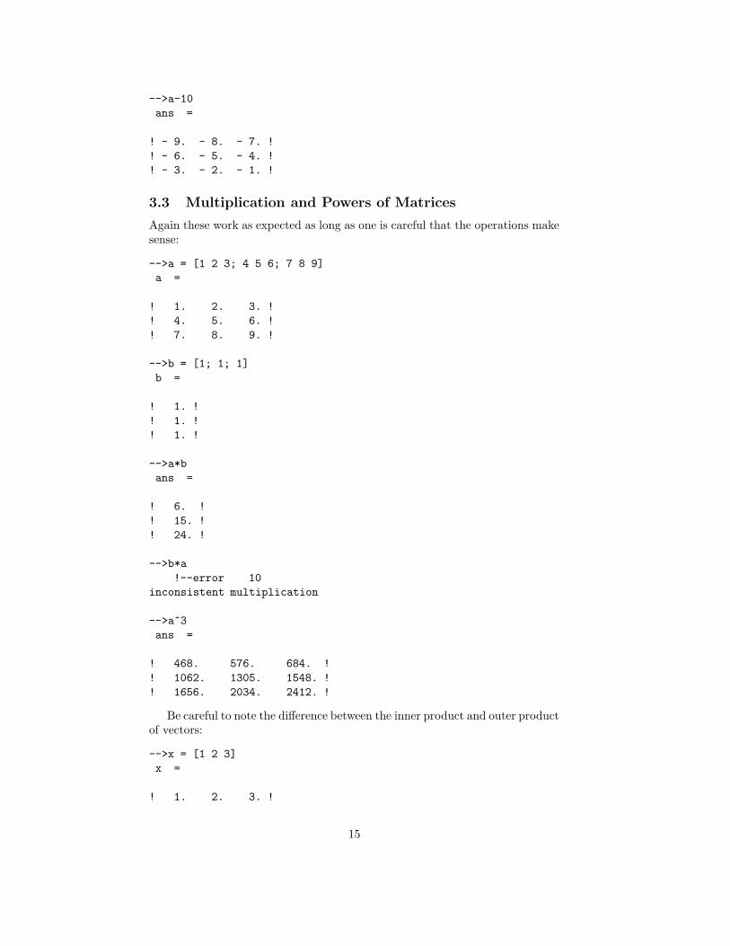
Note that in this example [sin(x) cos(x)] is a two column matrix.

5.4 Multiple Plots

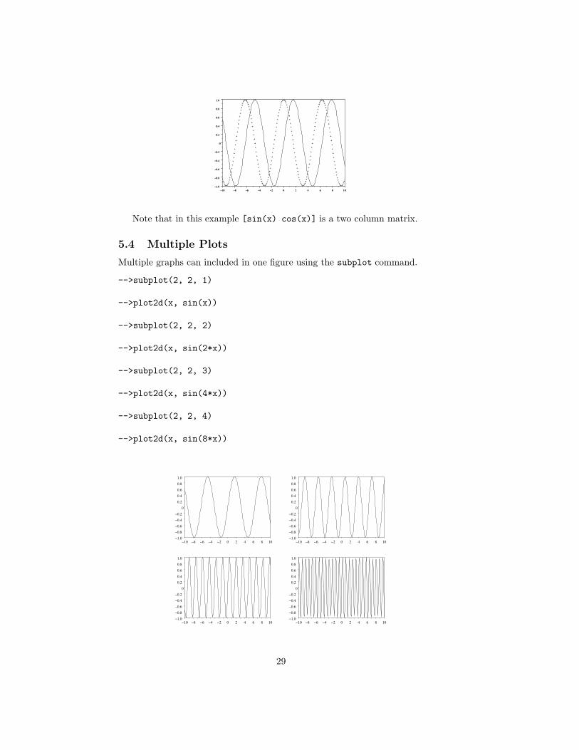
Multiple graphs can included in one figure using the subplot command.

-->subplot(2, 2, 1)

-->plot2d(x, sin(x))

-->subplot(2, 2, 2)

-->plot2d(x, sin(2*x))

-->subplot(2, 2, 3)

-->plot2d(x, sin(4*x))

-->subplot(2, 2, 4)

-->plot2d(x, sin(8*x))

−10 −8 −6 −4 −2 0 2 4 6 8 10−1.0−0.8−0.6−0.4−0.2

00.20.40.60.81.0

−10 −8 −6 −4 −2 0 2 4 6 8 10−1.0−0.8−0.6−0.4−0.2

00.20.40.60.81.0

−10 −8 −6 −4 −2 0 2 4 6 8 10−1.0−0.8−0.6−0.4−0.2

00.20.40.60.81.0

−10 −8 −6 −4 −2 0 2 4 6 8 10−1.0−0.8−0.6−0.4−0.2

00.20.40.60.81.0

29

5.5 Other Features

There a lot of things Scilab can do with graphs. Here is an example. See thehelp pages for more information.

-->plot2d(x, sin(x)./x, rect = [-20 -0.5 20 1.5], ...

--> axesflag = 5, nax = [10 4 5 4])

−20 −10 0 10 20

−0.5

0.0

0.5

1.0

1.5

5.6 3D Curves

Curves in 3 dimensional space can be plotted using param3d. It takes threevectors containing the values the x, y and z coordinates of the points on thecurve. By clicking on the 3D Rot button on the graphics window and playingaround with the mouse you can alter the orientation of the graph.

-->z = (0:.01:10)’;

-->param3d(z.*sin(5*z), z.*cos(5*z), z)

10

5

0

Z

9.1

−0.3

−9.7X

−9.4

0.1

9.6

Y

5.7 Histograms

Histograms can be plotted with the histplot(n, data) command. Here n isthe number of bins in the histogram and data is the vector of data for which

30

we want to draw the histogram. The following example draws a histogram of avector of normally distributed random numbers.

-->rr = rand(1, 10000, ’normal’);

-->histplot(40, rr)

−4 −3 −2 −1 0 1 2 3 40

0.1

0.2

0.3

0.4

0.5

6 Working with Files in Scilab

To work with external files in Scilab, both you and Scilab need to know wherethese files are. This is particularly important when creating and editing scriptand function files (see below).

Linux

There will be no problems if you start your text editor and Scilab in the samedirectory. Recent versions of Scilab have a built-in text editor.

Windows

The Windows version of Scilab has a built-in text editor. By default, this editorsaves files in the folder Documents and Settings. you need remember this ifyou want to access these files from another program.

6.1 Function Files

Functions can be typed directly into Scilab as in the examples in §4.2. Functionfiles contain one or more function definitions like the functions hilbert andfactorial in §4.2. It is common to put functions in files rather than enterthem directly into Scilab since (a) they are then saved away for further use, and(b) it is easy to correct or modify a function by editing the file.

Create a file, say hilbert.sci (it is usual but not mandatory to end functionfiles with the suffix .sci), containing the function above:

31

function h = hilbert(n)

h = zeros(n,n)

for i = 1:n

for j = 1:n

h(i,j) = 1/(i + j - 1)

end

end

endfunction

Once a function file is loaded with the exec command, the functions in thefile are avilable:

-->exec("hilbert.sci");

-->hilbert(4)

ans =

! 1. 0.5 0.3333333 0.25 !

! 0.5 0.3333333 0.25 0.2 !

! 0.3333333 0.25 0.2 0.1666667 !

! 0.25 0.2 0.1666667 0.1428571 !

6.2 Script Files

Script files are like function files except that they contain any sort of Scilabcommands. When the file is loaded by the exec command the commands in fileexecuted as if they are typed directly into Scilab. There are two main uses forscript files:

1. To repeat a series of commands, often to perform a numerical experiment.

2. To enter largish problems into Scilab. Here the use of script files allows usto correct errors by editing a file rather than retyping the whole probleminto Scilab.

6.3 Exporting Data

The write command writes Scilab data to external files, which can then be usedby other programs. Here is an example:

-->z = rand(8,4)

z =

! 0.2113249 0.8782165 0.2312237 0.3616361 !

! 0.7560439 0.0683740 0.2164633 0.2922267 !

! 0.0002211 0.5608486 0.8833888 0.5664249 !

! 0.3303271 0.6623569 0.6525135 0.4826472 !

! 0.6653811 0.7263507 0.3076091 0.3321719 !

! 0.6283918 0.1985144 0.9329616 0.5935095 !

! 0.8497452 0.5442573 0.2146008 0.5015342 !

! 0.6857310 0.2320748 0.312642 0.4368588 !

-->write("out1.dat", z)

32

If you examine the file out1.dat it will look something like:

0.211324865 0.878216481 0.23122372 0.361636101

0.756043854 0.0683740368 0.216463263 0.292226664

0.000221134629 0.560848606 0.883388781 0.566424882

0.330327092 0.662356937 0.652513495 0.482647197

0.665381104 0.726350677 0.307609074 0.332171891

0.628391788 0.198514384 0.932961621 0.59350947

0.849745236 0.544257316 0.214600786 0.50153416

0.68573102 0.23207479 0.312641997 0.436858758

Note that only one matrix can be written to a file at any one time.

6.4 Importing Data

The read command is used to read data from external files into a Scilab matrix.We can read the data we wrote to a file in the previous example:

-->z1 = read("out1.dat", 8, 4)

z1 =

! 0.2113249 0.8782165 0.2312237 0.3616361 !

! 0.7560439 0.0683740 0.2164633 0.2922267 !

! 0.0002211 0.5608486 0.8833888 0.5664249 !

! 0.3303271 0.6623569 0.6525135 0.4826472 !

! 0.6653811 0.7263507 0.3076091 0.3321719 !

! 0.6283918 0.1985144 0.9329616 0.5935095 !

! 0.8497452 0.5442573 0.2146008 0.5015342 !

! 0.6857310 0.2320748 0.312642 0.4368588 !

The matrix z1 is not the same as the matrix z since we saw that the datafrom z was written with only about 9 digits:

-->z1-z

ans =

1.0E-10 *

! - 4.641211 - 3.0193348 3.3980727 1.9742941 !

! - 1.695476 - 0.1129218 - 1.4657928 2.0935681 !

! - 0.0010056 - 2.8470781 - 4.5441417 4.2623349 !

! 2.6141833 - 3.0413916 2.8490543 - 3.2105735 !

! - 2.1970492 2.6599956 - 2.8339125 - 3.5029912 !

! - 3.4110503 - 2.175603 - 3.2173775 - 1.126218 !

! 1.2847634 - 2.7270575 - 1.0107304 2.3907776 !

! 1.752567 2.971077 1.0969353 - 3.3034514 !

The read statement has the general form

x = read(filename, nrows, ncols)

33

and read assumes that the data in the file it is reading is organized in columns.However the number of rows, nrows, and number of columns, ncols in the readstatement doesn’t have to match the layout of the data in the file.

Here are some examples:

-->z2 = read("out1.dat", 3, 3)

z2 =

! 0.2113249 0.8782165 0.2312237 !

! 0.7560439 0.0683740 0.2164633 !

! 0.0002211 0.5608486 0.8833888 !

-->z3 = read("out1.dat", 2, 5)

z3 =

! 0.2113249 0.8782165 0.2312237 0.3616361 0.7560439 !

! 0.0002211 0.5608486 0.8833888 0.5664249 0.3303271 !

-->z4 = read("out1.dat", -1, 4)

z4 =

! 0.2113249 0.8782165 0.2312237 0.3616361 !

! 0.7560439 0.0683740 0.2164633 0.2922267 !

! 0.0002211 0.5608486 0.8833888 0.5664249 !

! 0.3303271 0.6623569 0.6525135 0.4826472 !

! 0.6653811 0.7263507 0.3076091 0.3321719 !

! 0.6283918 0.1985144 0.9329616 0.5935095 !

! 0.8497452 0.5442573 0.2146008 0.5015342 !

! 0.6857310 0.2320748 0.312642 0.4368588 !

In the first example above, we just read the first three rows and columns ofthe data. In the second example the first ten data values were read into a 2× 5matrix. If you know the number of columns in a data file, you can simply use-1 for the number of rows and all rows of the data will be read.

7 Scilab Internals

7.1 The Environment

Whenever you define new variables, e.g. by something like x = 10, or newfunctions, they are saved in the environment together with a largish number ofbuilt-in variables, functions and libraries. The command

-->whos()

prints a list of what is in the environment, with the user defined variables andfunctions first. This is useful if you want to know what names you have usedand what type and size of data is associated with those names.

34

7.2 Saving and Restoring the Environment

Saving and restoring the environment between Scilab sessions can be done withthe commands save and load. For example the current environment can besaved in file work.dat with the command

-->save("work.dat")

and then later restored with

-->load("work.dat")

The file produced by the save is a binary file which cannot be used in anysensible way by other programs.

If you only want to save a few variables or functions, say a, b and c, thenthe variation

-->save("work.dat", a, b, c)

saves only the named objects.

7.3 The Stack

Scilab uses an internal stack for its calculations and to store the variables in theenvironment. You can find the size of the stack as follows:

-->stacksize()

ans =

! 1000000. 117893. !

These two numbers are the size of the stack and the amount of the stack in use,both measured in 64 bit (double precision) words.

It can happen that very large matrices are too big for the stack in whichcase an error is signalled:

-->rr = rand(1000,1000);

!--error 17

rand: stack size exceeded (Use stacksize function to increase it)

The matrix rr has a million elements, which to big for the current stack.Given that the current stacksize is also one million, to work with rr we

should at least double the size of the stack:

-->stacksize(2000000)

-->stacksize()

ans =

! 2000000. 119087. !

-->rr = rand(1000,1000);

-->stacksize()

ans =

! 2000000. 1019091. !

35