Notes on Queueing Theory and Simulation

Dr. Deep Medhi, University of Missouri-Kansas City

Notes on Queueing Theory

Chapter 2:Stochastic Processes, B-D Model and Queues

In this section, we provide brief overview of stochastic processes, and then go into birth-and-death

model and queueing analysis. You may want to consult the book by Allen [1] (used often in CS 394) for

more material on stochastic processes etc.

1. Stochastic ProcessesLet t be a parameter, assuming values in a set T . Let A�t� be a random or stochastic variable for every

t � T . The family fA�t�jt � Tg is called a stochastic process.

We think about stochastic events that occur over time, i.e, t is in time-space. In terms of measurement,

we can quantify time as either a continuous variable or a discrete variable. (for example the ALOHA protocol

uses continuous time model while slotted ALOHA uses discrete time model.) Similarly, the state space

(values for the stochastic process) can also be continuous (C) or discrete (D). The possible combinations

are:

Time state-space

C D to discuss

C C e.g. brownian motion - not covered

D C Waiting time of n-th arrival in a queue

D D to discuss

In discrete state space, the stochastic process is called a chain with values denoted, e.g., S �

f�� �� ����mg.

2. Discrete-time Markov chainA stochastic process fAn� n � �g is called a Markov chain if for every xi � S, we have

PrfAn � xnjAn�� � xn�� � ���A� � x�g � PrfAn � xnjAn�� � xn��g�

(In this definition, we use time to be discrete.) What this means is that for a Markov chain, the

probability at time n depends only on the previous state and nothing before that. This is known as the

memoryless property of a Markov chain.

Now, what is the probability of the process being in state j given that it was in state i in the preceding

time? This is the transition probability from state i to j. It is written as:

CS 522, v 0.94, d.medhi, W’99 5

pij � PrfAn � jjAn�� � ig

Given, you are at state i at time n � �, the probabilities of moving to all states (in the next time slot)

must add up to 1, i.e.

�X

j��

pij � �� for each i�

A Markov chain is called temporally homogeneous if :

PrfAn � jjAn�� � ig � PrfAn�m � jjAn�m�� � ig�

The transition probability is then denoted by pij . For all possible values of i� j, one can denote he the

transition probability as a matrix with elements �pij�.

The transition in n-step is given by

pij�n� � PrfAn � jjA� � ig�

Since a Markov chain has stationary transition probabilities, we have

pij�n� � PrfAm�n � jjAm � ig for all m � � and n � ��

3. Continuous-time, Markov ChainLet fX�t�� � � t � �g be a Markov process with countable state space S � f�� �� �� ���g over

continuous time-space t. For, example, X�t� can be the number of customers in the system at time t. For

continuous time, discrete space (Markov chains) the transition probability is denoted by,

pij�t� � Prfx�t � u� � jjx�u� � ig� t � �� i� j � S

Note, X

j

pij�t� � �� for each i�

Now, we can consider all the possible cases for i� j at time t giving us a matrix of information. Thus,

in matrix notation,

P �t� �� �pij�t� �� transition probability matrix�

CS 522, v 0.94, d.medhi, W’99 6

4. Chapman-Kolmogorov equationSo far we have mentioned one-step transition probabilities, i.e., probability of An given An�� . C-K

equation provides a relation for multiple steps as follows:

pij�n� m� �X

k

pik�n�pkj�m�� ���

where n�m � �� �� �� ���.

For continuous time, this can be written as:

pij�s� t� �X

k

pik�s�pkj�t�� ���

where s� t � ��

In matrix notation,

P �s � t� � P �s�P �t��

Set the initial transition probability matrix as

P ��� � I (identity matrix)

i.e.,

pij��� � � if i � j� else � if i �� j�

Define,

qij �� limt��

pij�t�� pij���

t� lim

t��

pij�t�

t� for j �� i�

qii �� limt��

pii�t�� pii���

t� lim

t��

pii�t�� �

t�

Note that q’s are instantaneous rate. In matrix notation,

Q � limt��

P �t�� I

t�

where, Q � qij � Now, recall the relation

X

j

pij�t� � ��

If we move 1 from RHS to LHS of this equation and then divide by t and let t� �, we get

limt��

fpi��t��t� ������ �pii�t�� ���t� ����� pik�t��t� ���g � �

which implies

qi� � ������ qii � ������ qik � ��� � ��

CS 522, v 0.94, d.medhi, W’99 7

In short, we have X

j ��i

qij � qii � �� ���

Typically, we denote qii � �qi , thus, we have

X

j ��i

qij � qi�

The matrix, Q, is known as the transition density matrix, or, infinitesimal generator, or a rate matrix.

If the state space S is finite, then

Q �

�B��q� q�� ��� q�mq�� �q� ��� q�m

���

qm� qm� ��� �qm

�CA �

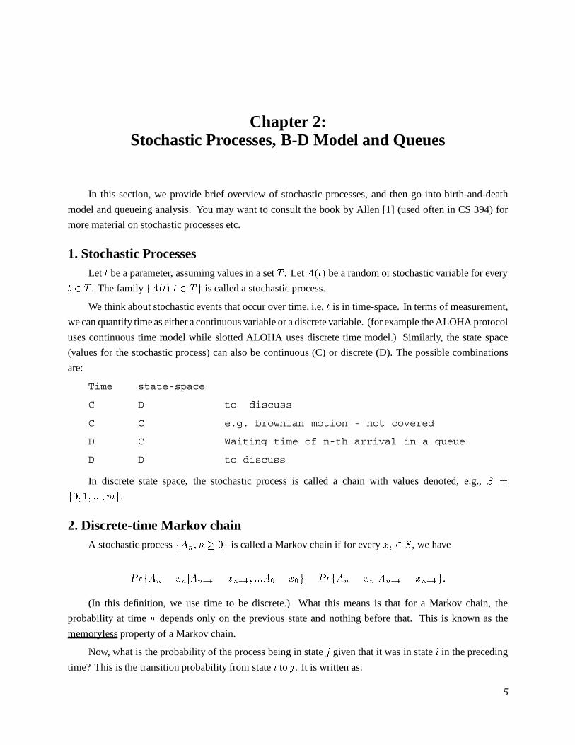
This is another way to write the C-K equation in terms of rate:

P ��t� �d�P �t��

dt� QP �t��

or,d�P �t��

dt� P �t�Q�

���

Now, consider the vector ��t� �� f���t�� ���t�� ���g� This is the probability vector of the state of the

system at time t, i.e., probability of being at state 0 in time t is ���t� etc.

Now, we move to the steady-state situation, i.e, what is the system going to be like in steady-state as

t� �.

It is easy to see that

��t� � ����P �t��

Also,d���t��

dt� ����P ��t� � ����P �t�Q � ��t�Q� ���

If we denote the steady-state probability vector by �, i.e.

� � limt��

��t�

then, from the relation (5) and letting t��, we get (since, derivative of a constant is zero),

� � �Q

with the requirement that probabilities sum up to 1

�� � �� � ��� � �

CS 522, v 0.94, d.medhi, W’99 8

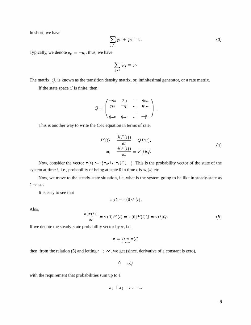
if e is a column vector of the same dimension as � with each component being 1, we can write this in

compact form as �e � �.

Note that

� � �Q� �e � � ���

is a linear system of equation which has a unique solution (under certain conditions).

To illustrate, suppose that we have a system that takes three values (0, 1, 2). The probabilities are:

� � ���� ��� ���

and �Q � � is

���� ��� ���

���q� q�� q��q�� �q� q��q�� q�� �q�

�� � �� � � �

and �e � � is

�� � �� � �� � ��

If we know q’s, then we can solve for �.

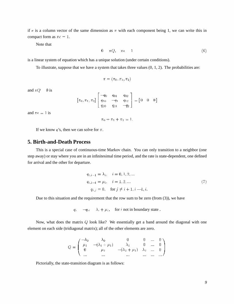
5. Birth-and-Death ProcessThis is a special case of continuous-time Markov chain. You can only transition to a neighbor (one

step away) or stay where you are in an infinitesimal time period, and the rate is state-dependent, one defined

for arrival and the other for departure.

qi�i�� � �i� i � �� �� � ���

qi�i�� � �i� i � �� � ���

qi�j � �� for j �� i� �� i� �� i�

��

Due to this situation and the requirement that the row sum to be zero (from (3)), we have

qi � �qii � �i � �i� for i not in boundary state �

Now, what does the matrix Q look like? We essentially get a band around the diagonal with one

element on each side (tridiagonal matrix); all of the other elements are zero.

Q �

�B���� �� � � ��� ��� ���� � ��� �� � ��� �� �� ���� � ��� �� ��� ���� ��� ��� ��� ��� ���

�CA

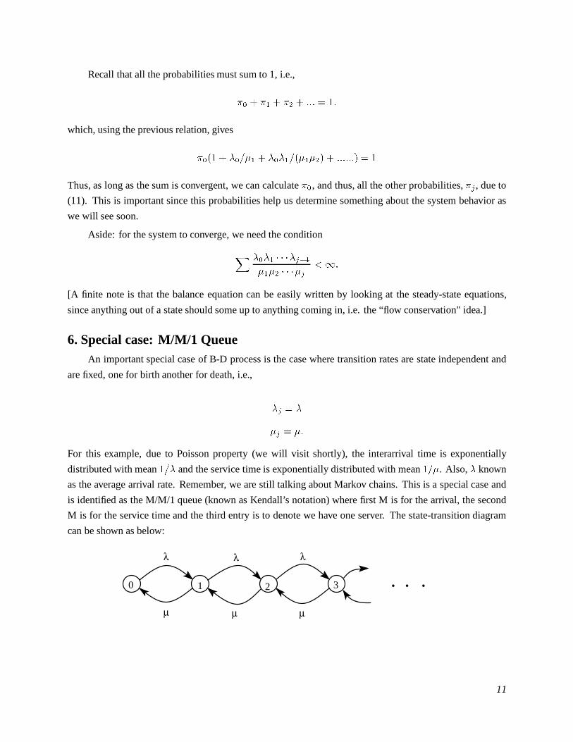
Pictorially, the state-transition diagram is as follows:

CS 522, v 0.94, d.medhi, W’99 9

• • •0 1 2 3

λ 0 λ1 λ 2

µ1 µ2 µ3

Now, let’s go back to C-K equation. For the birth-and-death process, we can rewrite the C-K equation

(from (4)) as

p�ij�t� � ���j � �j� pij�t� � �j��pi�j���t� � �j��pi�j���t�� for j � �

p�i��t� � ���pi��t� � ��pi���t�����

Suppose that �j’s and �i’s are non-zero. Then, the Markov chain is irreducible (means every state can

be reached from every other state by chaining), it can be shown that in steady-state

limt��

pij�t� � �j

exists and are independent of the initial state i.

Revisiting C-K equation above and using the fact that the derivative of a constant is zero, we have

� � ���j � �j� �j � �j���j�� � �j���j��� for j � � ���

� � ����� � ����� ����

These are also known as balance equations. In fact, the above is nothing but �Q � �, specialized for the

B-D model. The nice thing is that this linear system of equations is easily solvable analytically.

From (10), we have

�� ���

�����

For j � � from (9), we have

� � ���� � ��� �� � ���� � ����

which implies [using (10)],

���� � ���� � ���� � ���� � �����

Thus,

�� ���

���� �

����

�������

Generalizing, we get

�j ���������j��

��������j

��� j � �� ����

CS 522, v 0.94, d.medhi, W’99 10

Recall that all the probabilities must sum to 1, i.e.,

�� � �� � �� � ��� � ��

which, using the previous relation, gives

���� � ����� � ����������� � ������� � �

Thus, as long as the sum is convergent, we can calculate ��, and thus, all the other probabilities, �j , due to

(11). This is important since this probabilities help us determine something about the system behavior as

we will see soon.

Aside: for the system to converge, we need the condition

X ���� � � ��j��

���� � � ��j

���

[A finite note is that the balance equation can be easily written by looking at the steady-state equations,

since anything out of a state should some up to anything coming in, i.e. the “flow conservation" idea.]

6. Special case: M/M/1 QueueAn important special case of B-D process is the case where transition rates are state independent and

are fixed, one for birth another for death, i.e.,

�j � �

�j � ��

For this example, due to Poisson property (we will visit shortly), the interarrival time is exponentially

distributed with mean ��� and the service time is exponentially distributed with mean ���. Also, � known

as the average arrival rate. Remember, we are still talking about Markov chains. This is a special case and

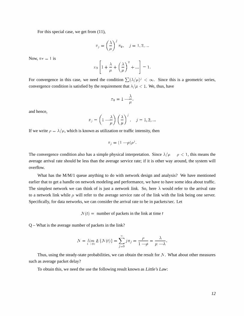
is identified as the M/M/1 queue (known as Kendall’s notation) where first M is for the arrival, the second

M is for the service time and the third entry is to denote we have one server. The state-transition diagram

can be shown as below:

• • •0 1 2 3

λ λ λ

µ µ µ

CS 522, v 0.94, d.medhi, W’99 11

For this special case, we get from (11),

�j �

��

�

�j

��� j � �� �� ���

Now, �e � � is

��

�� �

�

��

��

�

��� ���

�� ��

For convergence in this case, we need the conditionP�����j � �. Since this is a geometric series,

convergence condition is satisfied by the requirement that ��� � �. We, thus, have

�� � ���

��

and hence,

�j �

���

�

�

���

�

�j

� j � �� �� ���

If we write � � ���, which is known as utilization or traffic intensity, then

�j � ��� ���j�

The convergence condition also has a simple physical interpretation. Since ��� � � � �, this means the

average arrival rate should be less than the average service rate; if it is other way around, the system will

overflow.

What has the M/M/1 queue anything to do with network design and analysis? We have mentioned

earlier that to get a handle on network modeling and performance, we have to have some idea about traffic.

The simplest network we can think of is just a network link. So, here � would refer to the arrival rate

to a network link while � will refer to the average service rate of the link with the link being one server.

Specifically, for data networks, we can consider the arrival rate to be in packets/sec. Let

N�t� � number of packets in the link at time t

Q – What is the average number of packets in the link?

N � limt��

EfN�t�g ��Xj��

j�j ��

�� ��

�

� � ��

Thus, using the steady-state probabilities, we can obtain the result for N . What about other measures

such as average packet delay?

To obtain this, we need the use the following result known as Little’s Law:

CS 522, v 0.94, d.medhi, W’99 12

avg. number of packets in system in steady state (N)

= avg. arrival rate * avg. packet delay in system

in steady state (T)

That is,

N � �T�

Rearranging, we get

T � N�� ��

�� ��

�

���� ���

Average waiting time in the queue, W , is

W � Avg. waiting time in System – Avg. waiting time in Service ��

� � ��

�

��

�

� � ��

Again, by Little’s Law which is also applicable in queues, the average number of customers in queue is,

Nq � �W ���

�� ��

Thus, we have shown above four performance measures that may be of interest for a network link

which can be obtained once you know the average arrival rate and the average service rate.

Remark: An important assumption about the M/M/1 is that the input population is considered to be

infinite. In generic terms, the term ‘customer’ is used rather than packets since such models are applicable

in other areas besides communication networks.

We have discussed so far delay results for the average value only. How about 90-th percentile value?

For M/M/1, we have the following:

90-th percentile system delay = T ln�����

90-th percentile queueing delay = max fT ln������ �g�

Example # 1:

Suppose average arrival rate (�) is 100 pps, and the service rate (�) is 200 pps, then the average number

of packets in the system is N � ����� �� � ��������� ���� � ��

The following is a table for average number in the system and the average delay (in the system) for

different values of � and � (Note the impact on delay when � and � are scaled):

� � N T

100 200 1 10 ms

150 200 3 20 ms

175 200 7 40 ms

1000 2000 1 1 ms

1500 2000 3 2 ms

1750 2000 7 4 ms

CS 522, v 0.94, d.medhi, W’99 13

7. On exponential distributionThis is a good time to quickly go over a couple of things about exponential distribution. The pdf of the

exponential distribution with parameter � is given by

f�x� � �e��x� x � ��

The mean and the variance are given by

E�X� ��

�� V �X� �

�

���

8. Poisson ProcessA pure-birth homogeneous process, i.e., �j � �� �j � �, is a Poisson process. Another way:

A stochastic process fA�t�jt � �g taking non-negative integer values is said to be a Poisson process

with rate � if

1. fA�t�g is a counting process.

2. The number of arrival that occur in disjoint time interval are independent.

3. The number of arrivals in interval of length � is Poisson distributed with parameter ��

PrfA�t � ��� A�t� � ng � exp���������n�n�� n � �� �� ���

Note that exp is the exponential function, exp�x� � ex, where e is the Euler number (=2.718281828...).

Important properties of a Poisson process:

1) Interarrival times are independent and exponentially distributed with parameter �.

�n � tn�� � tn

Prf�n � sg � �� exp���s� � �� e��s�

2) Sum of two independent Poisson processes is a Poisson process with rate being the sum of the

two. This holds for more than two also.

It is important to note that the Poisson arrival can also be described by a pure-birth homogeneous

process.

CS 522, v 0.94, d.medhi, W’99 14

9. Revisiting a network linkIn the section on M/M/1, we mentioned why the results are applicable for a data network link. We

need to reiterate that M/M/1 results are applicable for Poisson arrival (discussed above) and exponentially

distributed service time.

Packet arrivals characterized by Poisson arrival is a reasonable assumption, although this is NOT always

a good one. However, this helps us get started on getting a handle on doing some analysis.

Typically, when we think of a network link we often have some idea about the rate such as 56 Kbps etc.

This is a deterministic rate. Now, how do we get exponentially distributed service time? In a link model,

the other factor that comes into the picture is the size of the packet that has arrived. Here is where we make

another assumption: the packet length is exponentially distributed with mean length ���� bits. Now if we

denote the speed of a link by C bps; then, the average service rate of packets is

� � ��C

which is exponentially distributed. Thus, we can use the M/M/1 model for exponentially distributed packet

size for studying a network link.

Example # 2:

If link speed is 1.5 Mbps (i.e., a T1-link), and the average packet size is 1 Kbits, then the average

service rate � is 1.5 Mbps/1Kbits = 1500 packets per sec (pps).

10. A view on Statistical MultiplexingThe next thing to realize is that all the packets that arrive to a data network link is statistically

multiplexed. This is a key behavior of packet-switched networks. This also results in queueing of packets

if all the capacity of a link is used up at a certain time – this points to the average packet delay we discussed

earlier.

Consider m statistically identical and independent Poisson packet streams each with an arrival rate of

��m packets per sec, transmitted over a communication link with exponentially distributed service time

with mean service rate �. In case of single “pipe", we have total Poisson arrival as m��m � � due to one

of properties of Poisson process mentioned earlier. Using M/M/1 model, we get the avg. delay to be

Ta ��

�� ��

If, in, the link is divided into m separate pipes (partitioned), then the service rate of each pipe is ��m, i.e.,

��m-th of the rate of the original pipe. In this case, the avg. delay (again using M/M/1 on one partition):

Tb ��

��m� ��m�

m

� � ��

Thus, splitting the line into m pipes increases the avg delay by m times! This is an interesting phenomenon

about statistical multiplexing; as a rule of thumb, it is better to have a fatter link than partition the link into

lower speeds since it results in more delay on average.

What about the effect on average number of packets due to the scenarios discussed here?

CS 522, v 0.94, d.medhi, W’99 15

11. Inverse problem: Find service rate for a given average delayWe now pay attention to the simplest design problem when just a single network link is considered.

We know that the average delay for M/M/1 model is given by:

T ��

�� ��

Suppose, you are given �, the offered traffic in arrival rate (based on forecasted data) and the requirement

that the average link delay should not be more than Tmax. To meet this delay, Tmax

, we need

�

�� �� Tmax

which implies:

� ��

Tmax� ��

Thus, we get a bound on the minimum service rate required to meet the requirement. Since service rate

corresponds to the link speed, this mean we can determine minimum link speed required if the average

packet size is known. Although this is a simple result, it ties offered traffic and QoS requirement to the

service rate to be provided.

Example # 3:

Suppose that the average arrival rate is 500 pps, and we are given that the average packet size is 4Kbits.

If the system goal is to provide an average delay of 30 ms or less, what should be the link speed?

Here ��ms � ����� �� � ����� ����. This implies that the service rate � is 533.33 pps or higher.

Since, the average packet size is 4 Kbits, the link speed needed is at least 2.13 Mbps or higher.

12. Finite Buffer System: M/M/1/BSo far, we have talked about M/M/1. Often, in reality, we do not have an infinite queue to hold all the

packets for transfer due to finite buffer size. Thus, another model of interest is the finite buffer system. How

is the system behavior under finite buffer scenario? Assume that the size of the finite buffer is B, including

server (but customer population is still infinite). That means, you can queue only up to B � �. If there is

an arrival when the buffer is full, then that arrival is dropped (lost); this is packet dropping due to buffer

overflow. Again, B-D model can be used here by catering specifically to this case. Here, the state-transition

diagram is as follows:

• • •0 1 2 3

λ λ λ

µ µ µ

B–1 B

λ

µ

and we have

CS 522, v 0.94, d.medhi, W’99 16

�j �

��� if � � j � B � �

�� otherwise.

�j �

��� if � � j � B

�� otherwise.

It can be derived (from B-D model or from the special case M/M/1) that

�j � �o

j��Yi��

�

�� ��

��

�

�j

� j � B ���� �� ���

and,

�� �

��� � BX

j��

��

�

�j

����

��� ���

�� �����B���

�� �

�� �B��� �� � ��� �� ��

For � � �, the following is true:

�j ��

B � �� j � B�

Note that the packet loss probability is given by �B .

The mean number of packets in the system:

N �BXj��

j�j ��

�� ��

�B � ���B��

�� �B���� �� ��

and

N � B�� if � � ��

The mean number of packets at the server, EfNsg, is:

EfNsg � PrfN � �gEfNsjN � �g� PrfN � �gEfNsjNs � �g

� �� � � � ��� ���� ��

Thus, the mean number of packets in the queue (for � �� �):

Nq � N �EfNsg � N � ��� ��� ��

�� �� �

� � B�B

�� �B���

while for � � �, we have

Nq � B�� �B��B � ���

Effective arrival rate is given by

�� � �

B��Xj��

�j � ���� �B��

The mean response time (average delay) is

T � N��� � N� ����� �B�� �

The mean waiting time is

W � Nq��� � Nq� ����� �B�� �

CS 522, v 0.94, d.medhi, W’99 17

13. M/M/m model: m parallel serversAnother model of interest in communication networks is m parallel servers. This model comes up in

the case of a communication link which is divided into m circuits or channels. An arriving customer can

take any of the circuits on arrival, OR, has to wait if all the servers (circuits) are busy. Infinite population

assumption is made here. [this model is close to a telephone network link, but not quite; we’ll see later

where the difference is].

This is again a B-D model, where

�j � ��

and

�j �

�j�� if � � j � m

m�� for j � m.

The state-transition diagram is

• • •0 1 2 3

λ λ λ

µ 2µ 3µ

m m+1

λ

mµmµ mµ

• • •

Note that for M/M/m model, the utilization, �, is

� ��

m�� ��

Here, we can show (from B-D model) that

�j �

����������

�j�

j���� for � � j � m

���

�j�

m�mj�m ��� for j � m.

Further,

�� �

�� �����m

m���� ���m����m��Xj��

�����j

j�

��

�

Given �’s, different performance measures can be derived.

CS 522, v 0.94, d.medhi, W’99 18

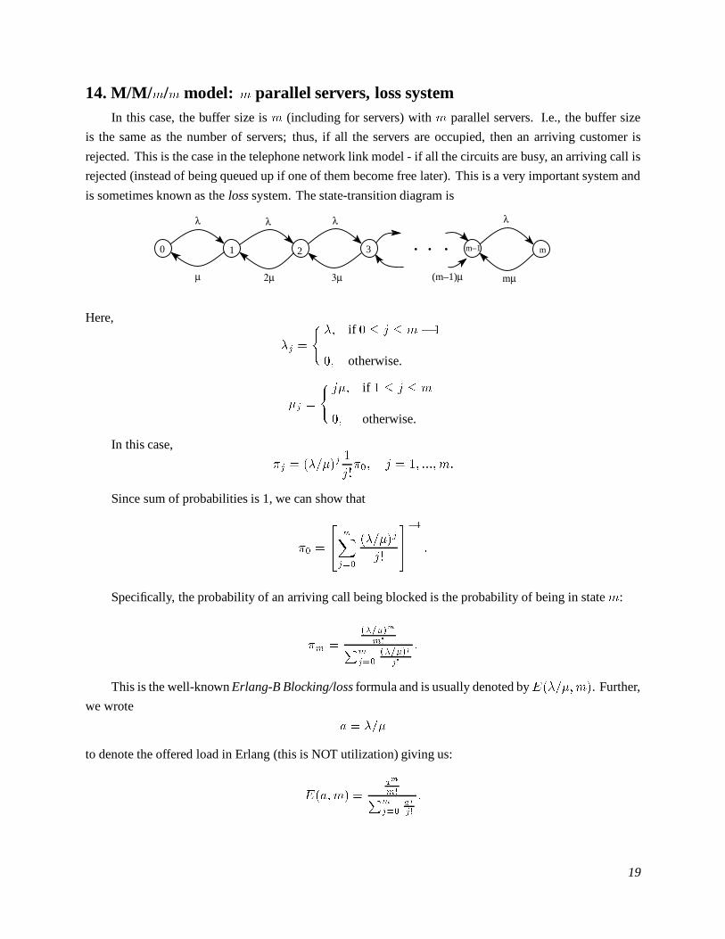
14. M/M/m/m model: m parallel servers, loss systemIn this case, the buffer size is m (including for servers) with m parallel servers. I.e., the buffer size

is the same as the number of servers; thus, if all the servers are occupied, then an arriving customer is

rejected. This is the case in the telephone network link model - if all the circuits are busy, an arriving call is

rejected (instead of being queued up if one of them become free later). This is a very important system and

is sometimes known as the loss system. The state-transition diagram is

• • •0 1 2 3

λ λ λ

µ 2µ 3µ

m–1 m

λ

mµ(m–1)µ

Here,

�j �

��� if � � j � m� �

�� otherwise.

�j �

� j�� if � � j � m

�� otherwise.

In this case,

�j � �����j�

j���� j � �� ���� m�

Since sum of probabilities is 1, we can show that

�� �

�� mXj��

�����j

j�

����

�

Specifically, the probability of an arriving call being blocked is the probability of being in state m:

�m ������m

m�Pmj��

�����j

j�

�

This is the well-known Erlang-B Blocking/loss formula and is usually denoted byE�����m�. Further,

we wrote

a � ���

to denote the offered load in Erlang (this is NOT utilization) giving us:

E�a�m� �am

m�Pmj��

aj

j�

�

CS 522, v 0.94, d.medhi, W’99 19

The average number in the system, N , is given by

N � a��� E�a�m���

It is interesting to note that the Erlang-B loss formual has the following recurrence relation:

E�a�m� �aE�a�m� ��

m� aE�a�m� ��

with the starting point B�a� �� � ��

This can also be computed iteratively: Write

E�a�m� � ��d�a�m��

Then,

d�a�m� � md�a�m� ���a� ��

Thus, the iteration to compute blocking given offered load of a erlangs and the number of channel, m,

is:

procedure erlangb (a, m)

d � �

for j � �� ���� m

d � j � d�a� �

endfor

b � ��d

return (b)

Note that here the offered load (traffic) is given in a erlangs. Recall our discussion at the end of chapter

1. We stated there that typically for telephone networks, we provide offered traffic as

Offered Load = Number of call attempts/ hour * average call holding time

On close scrutiny, this is ���, where ��� � average call holding time. Again note that the assumption of

arrival is Poisson. Further, we assume call holding time to be exponentially distributed.

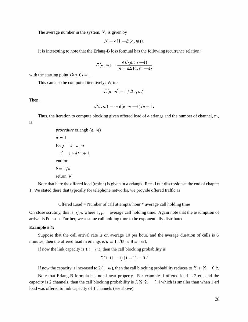
Example # 4:

Suppose that the call arrival rate is on average 10 per hour, and the average duration of calls is 6

minutes, then the offered load in erlangs is a � ������ � � �erl.

If now the link capacity is 1 (� m), then the call blocking probability is

E��� �� � ���� � �� � ���

If now the capacity is increased to 2 (� m), then the call blocking probability reduces toE��� �� � ���.

Note that Erlang-B formula has non-linear property. For example if offered load is 2 erl, and the

capacity is 2 channels, then the call blocking probability is E��� �� � �� which is smaller than when 1 erl

load was offered to link capacity of 1 channels (see above).

CS 522, v 0.94, d.medhi, W’99 20

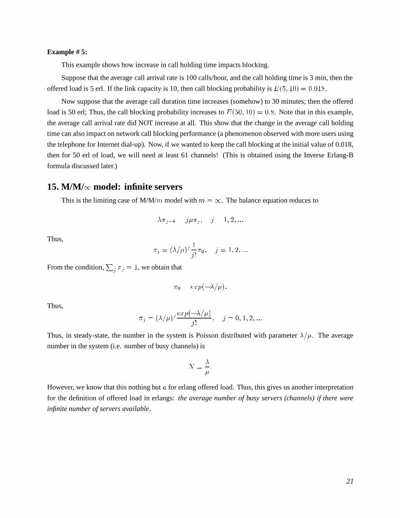
Example # 5:

This example shows how increase in call holding time impacts blocking.

Suppose that the average call arrival rate is 100 calls/hour, and the call holding time is 3 min, then the

offered load is 5 erl. If the link capacity is 10, then call blocking probability is E��� ��� � ������

Now suppose that the average call duration time increases (somehow) to 30 minutes; then the offered

load is 50 erl; Thus, the call blocking probability increases to E���� ��� � ���. Note that in this example,

the average call arrival rate did NOT increase at all. This show that the change in the average call holding

time can also impact on network call blocking performance (a phenomenon observed with more users using

the telephone for Internet dial-up). Now, if we wanted to keep the call blocking at the initial value of 0.018,

then for 50 erl of load, we will need at least 61 channels! (This is obtained using the Inverse Erlang-B

formula discussed later.)

15. M/M/� model: infinite serversThis is the limiting case of M/M/m model with m ��. The balance equation reduces to

��j�� � j��j � j � �� �� ���

Thus,

�j � �����j�

j���� j � �� �� ���

From the condition,P

j �j � �, we obtain that

�� � exp�������

Thus,

�j � �����jexp������

j�� j � �� �� �� ���

Thus, in steady-state, the number in the system is Poisson distributed with parameter ���. The average

number in the system (i.e. number of busy channels) is

N ��

��

However, we know that this nothing but a for erlang offered load. Thus, this gives us another interpretation

for the definition of offered load in erlangs: the average number of busy servers (channels) if there were

infinite number of servers available.

CS 522, v 0.94, d.medhi, W’99 21

16. M/M/1/ /K model: single server, finite populationIn this case, we have a finite population, K. The state-transition diagram is:

• • •0 1 2 3

Κ λ (Κ−1)λ (Κ−2)λ

µ µ µ

Κ−1 Κ

λ

µµ

2λ

In this case,

�j �

�����K � j�� if � � j � K

�� otherwise.

�j �

��� if � � j � K

�� otherwise.

Steady-state probabilities are given by

�j �K�

�K � j��

��

�

�j

��� � � j � K�

where

�� �

�� KXj��

��

�

�jK�

�K � j��

���

�

This model is often applicable for performance evaluation of a computer system where finite population

is a good assumption.

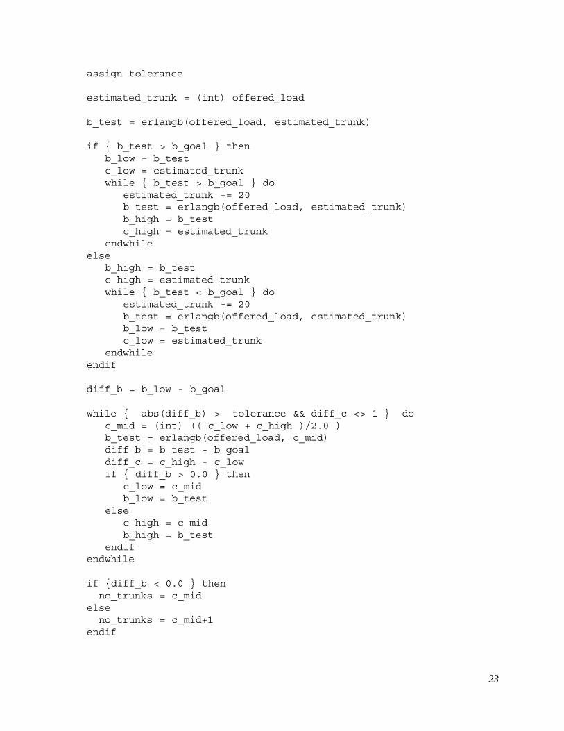
17. Inverse Erlang-B: given a and blocking, find the number of channelsThis is another inverse design problem for a network link where the offered load is given in erlangs

and the acceptable blocking level is also given, and we are to find the number of channels required in the

link to meet the acceptable level of blocking (known as grade-of-service).

The problem is to find an integral minimum m for given a and acceptable blocking b:

min fm E�a�m� � bg�

In this case, the inverse is not easy to calculate as in the M/M/1 case with delay. Thus, an algorithmic

approach is needed. We provide below a rough sketch:

Given offered_load and b_goal, estimate number of trunks========================================================

CS 522, v 0.94, d.medhi, W’99 22

assign tolerance

estimated_trunk = (int) offered_load

b_test = erlangb(offered_load, estimated_trunk)

if { b_test > b_goal } thenb_low = b_testc_low = estimated_trunkwhile { b_test > b_goal } do

estimated_trunk += 20b_test = erlangb(offered_load, estimated_trunk)b_high = b_testc_high = estimated_trunk

endwhileelse

b_high = b_testc_high = estimated_trunkwhile { b_test < b_goal } do

estimated_trunk -= 20b_test = erlangb(offered_load, estimated_trunk)b_low = b_testc_low = estimated_trunk

endwhileendif

diff_b = b_low - b_goal

while { abs(diff_b) > tolerance && diff_c <> 1 } doc_mid = (int) (( c_low + c_high )/2.0 )b_test = erlangb(offered_load, c_mid)diff_b = b_test - b_goaldiff_c = c_high - c_lowif { diff_b > 0.0 } then

c_low = c_midb_low = b_test

elsec_high = c_midb_high = b_test

endifendwhile

if {diff_b < 0.0 } thenno_trunks = c_mid

elseno_trunks = c_mid+1

endif

CS 522, v 0.94, d.medhi, W’99 23

Jagerman [5] presents a much elegant method where the number of channels is assumed to take

non-integral values.

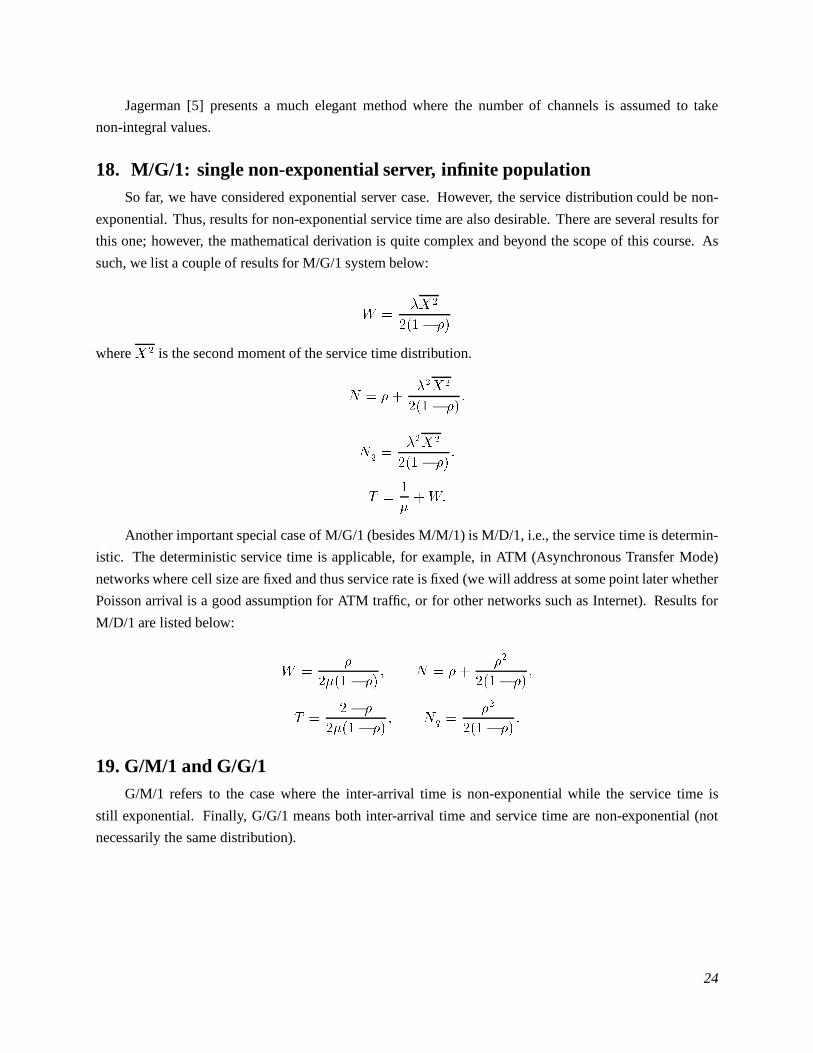
18. M/G/1: single non-exponential server, infinite populationSo far, we have considered exponential server case. However, the service distribution could be non-

exponential. Thus, results for non-exponential service time are also desirable. There are several results for

this one; however, the mathematical derivation is quite complex and beyond the scope of this course. As

such, we list a couple of results for M/G/1 system below:

W ��X�

���� ��

where X� is the second moment of the service time distribution.

N � ����X�

���� ���

Nq ���X�

���� ���

T ��

��W�

Another important special case of M/G/1 (besides M/M/1) is M/D/1, i.e., the service time is determin-

istic. The deterministic service time is applicable, for example, in ATM (Asynchronous Transfer Mode)

networks where cell size are fixed and thus service rate is fixed (we will address at some point later whether

Poisson arrival is a good assumption for ATM traffic, or for other networks such as Internet). Results for

M/D/1 are listed below:

W ��

����� ��� N � ��

��

���� ���

T ��� �

����� ��� Nq �

��

���� ���

19. G/M/1 and G/G/1G/M/1 refers to the case where the inter-arrival time is non-exponential while the service time is

still exponential. Finally, G/G/1 means both inter-arrival time and service time are non-exponential (not

necessarily the same distribution). More about this types of queues are left to courses such as CS 594 and

CS 694.

CS 522, v 0.94, d.medhi, W’99 24

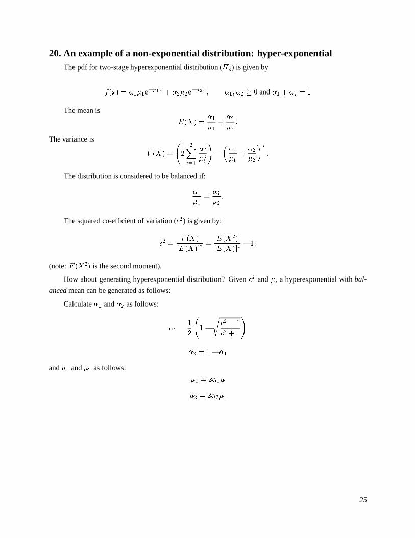
20. An example of a non-exponential distribution: hyper-exponentialThe pdf for two-stage hyperexponential distribution (H�) is given by

f�x� � ����e���x � ����e���x� ��� �� � � and �� � �� � �

The mean is

E�X� ���

�����

���

The variance is

V �X� �

��

�Xi��

�i

��i

��

���

�����

��

���

The distribution is considered to be balanced if:

��

���

��

���

The squared co-efficient of variation (c�) is given by:

c� �V �X�

�E�X����

E�X��

�E�X���� ��

(note: E�X�� is the second moment).

How about generating hyperexponential distribution? Given c� and �, a hyperexponential with bal-

anced mean can be generated as follows:

Calculate �� and �� as follows:

�� ��

�

���

rc� � �

c� � �

�

�� � �� ��

and �� and �� as follows:

�� � ����

�� � �����

CS 522, v 0.94, d.medhi, W’99 25

21. Considering M/M/1 and M/D/1 togetherIn the figures below, we plot N and T for different values of � for the systems M/M/1 and M/D/1.

Notice the difference as �� �.

utilization,0.1 0.2 0.3 0.4 0.5 0.6 0.7 0.8 0.9

0

20

40

60

80

100

120

T_mm1 T_md1

M/M/1 and M/D/1Average Delay

mu = 0.1

utilization,0.1 0.2 0.3 0.4 0.5 0.6 0.7 0.8 0.9

0

2

4

6

8

10

N_mm1 N_md1

M/M/1 and M/D/1Average number of customers in steady state

µ = 0.1

ρ

ρ

CS 522, v 0.94, d.medhi, W’99 26