Notes on pseudopotential generation - Quantum...

Notes on pseudopotential generation

Paolo GiannozziUniversita di Udine

URL: http://www.fisica.uniud.it/∼giannozz

October 23, 2017

Contents

1 Introduction 11.1 Who needs to generate a pseudopotential? . . . . . . . . . . . . . . . . 11.2 About similar work . . . . . . . . . . . . . . . . . . . . . . . . . . . . . 21.3 Pseudopotential generation, in general . . . . . . . . . . . . . . . . . . 2

2 Step-by-step Pseudopotential generation 32.1 Choosing the generation parameters . . . . . . . . . . . . . . . . . . . . 3

2.1.1 Exchange-correlation functional . . . . . . . . . . . . . . . . . . 32.1.2 Valence-core partition . . . . . . . . . . . . . . . . . . . . . . . 42.1.3 Electronic reference configuration . . . . . . . . . . . . . . . . . 52.1.4 Nonlinear core correction . . . . . . . . . . . . . . . . . . . . . . 6

2.2 Type of pseudization . . . . . . . . . . . . . . . . . . . . . . . . . . . . 72.2.1 Pseudization energies . . . . . . . . . . . . . . . . . . . . . . . . 72.2.2 Pseudization radii . . . . . . . . . . . . . . . . . . . . . . . . . . 82.2.3 Choosing the local potential . . . . . . . . . . . . . . . . . . . . 8

2.3 Generating the pseudopotential . . . . . . . . . . . . . . . . . . . . . . 92.4 Checking for transferability . . . . . . . . . . . . . . . . . . . . . . . . 10

3 A worked example: Ti 103.1 Single-projector, norm-conserving, no semicore . . . . . . . . . . . . . . 11

3.1.1 Generation . . . . . . . . . . . . . . . . . . . . . . . . . . . . . 113.1.2 Testing . . . . . . . . . . . . . . . . . . . . . . . . . . . . . . . . 15

3.2 Single-projector, norm-conserving, with semicore states . . . . . . . . . 193.3 Testing in molecules and solids . . . . . . . . . . . . . . . . . . . . . . 22

A Atomic Calculations 22A.1 Nonrelativistic case . . . . . . . . . . . . . . . . . . . . . . . . . . . . . 22

A.1.1 Useful formulae . . . . . . . . . . . . . . . . . . . . . . . . . . . 23A.2 Fully relativistic case . . . . . . . . . . . . . . . . . . . . . . . . . . . . 23A.3 Scalar-relativistic case . . . . . . . . . . . . . . . . . . . . . . . . . . . 23A.4 Numerical solution . . . . . . . . . . . . . . . . . . . . . . . . . . . . . 24

1

B Equations for the Troullier-Martins method 25

1 Introduction

When I started to do my first first-principle calculation (that is, my first2-principlecalculation) with Stefano Baroni on CsI under pressure (1985), it became quickly evi-dent that available pseudopotentials (PP’s) couldn’t do the job. So we generated ourown PP’s. Since that first experience I have generated a large number of PP’s andpeople keep asking me new PP’s from time to time. I am happy that ”my” PP’s areappreciated and used by other people. I don’t think however that the generation ofPP’s is such a hard task that it requires an official (or unofficial) PP wizard to do this.For this reason I want to share here my (little) experience.

These notes are written in general but having in mind the capabilities of the atomicpackage, included in the Quantum ESPRESSO distribution (http://www.quantum-espresso.org).atomic, mostly written and maintained by Andrea Dal Corso and others, is the evolu-tion of an older code I maintained for several years. atomic can generate both Norm-Conserving (NC) [1] and Ultrasoft (US) [2] PP’s, plus Projector Augmented Waves(PAW) [3] sets. It allows multiple projectors, full relativistic calculations, spin-splitPP’s for spin-orbit calculations. For the complete description of the input of atomic,please refer to files INPUT LD1.txt and INPUT LD1.html.

1.1 Who needs to generate a pseudopotential?

There are at least three well-known published sets of NC-PP’s: those of Bachelet,Hamann, and Schluter [4], those of Gonze, Stumpf, and Scheffler [5], and those ofGoedecker, Teter, and Hutter [6]. Moreover, all major packages for electronic-structurecalculations include a downloadable table of PP’s. One could then wonder what a PPgeneration code is useful for. The problem is that sometimes available PP’s will notsuit your needs. For instance, you may want:

– a better accuracy;

– PP’s generated with some exotic or new exchange-correlation functional;

– a different partition of electrons into valence and core;

– “softer” PP’s (i.e. PP that require a smaller cutoff in plane-wave calculations);

– PP’s with a core-hole for calculations of X-ray Adsorption Spectra;

– all-electron wavefunctions reconstruction (requires the knowledge of atomic all-electron and pseudo-orbitals used in the generation of PP’s);

or you may simply want to know what is a PP, how to produce PP’s, how reliable theyare.

1.2 About similar work

There are other PP generation packages available on-line. Those I am aware of include:

• the code by Jose-Luıs Martins et al.[7]:http://bohr.inesc-mn.pt/~jlm/pseudo.html

• the fhi98PP package[8]:http://www.fhi-berlin.mpg.de/th/fhi98md/fhi98PP

• the OPIUM code by Andrew Rappe et al.[9]:http://opium.sourceforge.net/

• David Vanderbilt’s US-PP package [2]:http://www.physics.rutgers.edu/~dhv/uspp/index.html.

Other codes may be available upon request from the authors.Years ago, it occurred to me that a web-based PP generation tool would have been

nice. Being too lazy and too ignorant in web-based applications, I did nothing. Irecently discovered that Miguel Marques et al. have implemented something like this:see http://www.tddft.org/programs/octopus/pseudo.php.

1.3 Pseudopotential generation, in general

In the following I am assuming that the basic PP theory is known to the reader.Otherwise, see Refs.[1, 4, 7, 8, 9] and references quoted therein for NC-PP’s; Refs.[2, 3]for US-PP’s and PAWsets. I am also assuming that the generated PP’s are to be usedin separable form [10] with a plane-wave (PW) basis set.

The PP generation is a three-step process. First, one generates atomic levels andorbitals with Density-functional theory (DFT). Second, from atomic results one gener-ates the PP. Third, one checks whether the reesulting PP is actually working. If not,one tries again in a different way.

The first step is invariably done assuming a spherically symmetric self-consistentHamiltonian, so that all elementary quantum mechanics results for the atom apply. Theatomic state is defined by the ”electronic configuration”, one-electron states are definedby a principal quantum number and by the angular momentum and are obtained bysolving a self-consistent radial Schrodinger-like (Kohn-Sham) equation.

The second step exists in many variants. One can generate “traditional” single-projector NC-PP’s; multiple-projector US-PP’s, or PAW sets. The crucial step is inall cases the generation of smooth “pseudo-orbitals” from atomic all-electron (AE)orbitals. Two popular pseudization methods are presently implemented: Troullier-Martins [7] and Rappe-Rabe-Kaxiras-Joannopoulos [9] (RRKJ).

The second and third steps are closer to cooking than to science. There is a largearbitrariness in the preceding step that one would like to exploit in order to get the”best” PP, but there is no well-defined way to do this. Moreover one is often forced tostrike a compromise between transferability (thus accuracy) and hardness (i.e. com-puter time). These two steps are the main focus of these notes.

2 Step-by-step Pseudopotential generation

If you want to generate a PP for a given atom, the checklist is the following:

• choose the generation parameters:

1. exchange-correlation functional

2. valence-core partition

3. electronic reference configuration

4. nonlinear core correction

5. type of pseudization

6. pseudization energies

7. pseudization radii

8. local potential

• generate the pseudopotential

• check for transferability

In case of trouble or of unsatisfactory results, one has to go back to the first step andchange the generation parameters, usually in the last four items.

2.1 Choosing the generation parameters

2.1.1 Exchange-correlation functional

PP’s must be generated with the same exchange-correlation (XC) functional that willbe later used in calculations. The use of, for instance, a GGA (Generalized GradientApproximation) functional tegether with PP’s generated with Local-Density Approx-imation (LDA) is inconsistent. This is why the PP file contains information on theDFT level used in their generation: if you or your code ignore it, you do it at your ownrisk.

The atomic package allows PP generation for a large number of functionals, bothLDA and GGA. Most of them have been extensively tested, but beware: some exoticor seldom-used functionals might contain bugs. Currently, atomic does not allow PPgeneration with meta-GGA (TPSS) or hybrid functionals. For the former, an oldversion of atomic, modified by Xiaofei Wang, is available. Work is in progress for thelatter.

Some functionals may present numerical problems when the charge density goesto zero. For instance, the Becke gradient correction to the exchange may diverge forρ→ 0. This does not happen in a free atom if the charge density behaves as it should,that is, as ρ(r)→ exp(−αr) for r →∞. In a pseudoatom, however, a weird behaviormay arise around the core region, r → 0, because the pseudocharge in that region is verysmall or sometimes vanishing (if there are no filled s states). As a consequence, nasty-looking “spikes” appear in the unscreened pseudopotential very close to the nucleus.This is not nice at all but it is usually harmless, because the interested region is really

very small. However in some unfortunate cases there can be convergence problems. Ifyou do not want to see those horrible spikes, or if you experience problems, you havethe following choices:

– Use a better-behaved GGA, such as PBE

– Use the nonlinear core correction, which ensures the presence of some chargeclose to the nucleus.

A further possibility would be to cut the gradient correction for small r (it used to beimplemented, but it isn’t any longer).

2.1.2 Valence-core partition

This seems to be a trivial step, and often it is: valence states are those that contributeto bonding, core states are those that do not contribute. Things may sometimes bemore complicated than this. For instance:

– in transition metals, whose typical outer electronic configuration is somethinglike (n = main quantum number) ndi(n+ 1)sj(n+ 1)pk, it is not always evidentthat the ns and np states (“semicore states”) can be safely put into the core.The problem is that nd states are localized in the same spatial region as ns andnp states, deeper than (n + 1)s and (n + 1)p states. This may lead to poortransferability. Typically, PP’s with semicore states in the core work well insolids with weak or metallic bonding, but perform poorly in compounds with astronger (chemical) type of bonding.

– Heavy alkali metals (Rb, Cs, maybe also K) have a large polarizable core. PP’swith just one electron may not always give satisfactory results.

– In some II-VI and III-V semiconductors, such as ZnSe and GaN, the contributionof the d states of the cation to the bonding is not negligible and may requireexplicit inclusion of those d states into the valence.

In all these cases, promoting the highest core states ns and np, or nd, into valence maybe a computationally expensive but obliged way to improve poor transferability. .

You should include semicore states into valence only if really needed: their inclusionin fact makes your PP harder (unless you resort to US pseudization) and increases thenumber of electrons. In principle you should also use more than one projector perangular momentum, because the energy range to be covered by the PP with semicoreelectrons is much wider than without. For instance, it may happen that the erroron the lattice parameter of a simple metal is larger with a semicore PP than with avalence-only PP.

2.1.3 Electronic reference configuration

This may be any reasonable configuration not too far away from the expected configu-ration in solids or molecules. As a first choice, use the atomic ground state, unless youhave a reason to do otherwise, such as for instance:

– You do not want to deal with unbound states. Very often states with highestangular momentum l are not bound in the atom (an example: the 3d state in Siis not bound on the ground state 3s23p2, at least with LDA or GGA). In such acase one has the choice between

– using one configuration for s and p, another, more ionic one, for d, as inRefs.[4, 5];

– choosing a single, more ionic configuration for which all desired states arebound;

– generate PP’s on unbound states: requires to choose a suitable referenceenergy.

– The results of your PP are very sensitive to the chosen configuration. This issomething that in principle should not happen, but I am aware of at least onecase in which it does. In III-V zincblende semiconductors, the equilibrium latticeparameter is rather sensitive to the form of the d potential of the cation (due tothe presence of p − d coupling between anion p states and cation d states [12]).By varying the reference configuration, one can change the equilibrium latticeparameter by as much as 1 − 2%. The problem arises if you want to calculateaccurate dynamical properties of GaAs/AlAs alloys and superlattices: you needto get a good theoretical lattice matching between GaAs and AlAs, or otherwiseunpleasant spurious effects may arise. When I was confronted with this problem,I didn’t find any better solution than to tweak the 4d reference configuration forGa until I got the observed lattice-matching.

– You know that for the system you are interested in, the atom will be in a givenconfiguration and you try to stay close to it. This is not very elegant but some-times it is needed. For instance, in transition metals described by a PP withsemicore states in the core, it is probably wise to chose an electronic configura-tion for d states that is close to what you expect in your system (as a hand-waivingargument, consider that the (n+ 1)s and (n+ 1)p PP have a hard time in repro-ducing the true potential if the nd state, which is much more localized, changes alot with respect to the starting configuration). In Rare-Earth compounds, leav-ing the 4f electrons in the core with the correct occupancy (if known) may be aquick and dirty way to avoid the well-known problems of DFT yielding the wrongoccupancy in highly correlated materials.

– You don’t manage to build a decent PP with the ground state configuration, forwhatever reason.

NOTE 1: you can calculate PP for a l as high as you want, but you are not obligedto use all of them in PW calculations. The general rule is that if your atom has statesup to l = lc in the core, you need a PP with angular momenta up to l = lc+1. Angularmomenta l > lc+1 will feel the same potential as l = lc+1, because for all of them thereis no orthogonalization to core states. As a consequence a PP should have projectorson angular momenta up to lc; l = lc + 1 should be the local reference state for PWcalculations. This rule is not very strict and may be relaxed: high angular momenta

are seldom important (but be careful if they are). Moreover separable PP pose seriousconstraints on local reference l (see below) and the choice is sometimes obliged. Notealso that the highest the l in the PP, the more expensive the PW calculation will be.

NOTE 2: a completely empty configuration (s0p0d0) or a configuration with frac-tional occupation numbers are both acceptable. Even if fractional occupation numbersdo not correspond to a physical atomic state, they correspond to a well-defined math-ematical object.

NOTE 3: PP could in principle be generated on a spin-polarized configuration, buta spin-unpolarized one is typically used. Since PP are constructed to be transferrable,they can describe spin-polarized configurations as well. The nonlinear core correctionis needed if you plan to use PP in spin-polarized (magnetic) systems.

2.1.4 Nonlinear core correction

The nonlinear core correction[11] accounts at least partially for the nonlinearity in theXC potential. During PP generation one first produces a potential yielding the desiredpseudo-orbitals and pseudoenergies. In order to extract a “bare” PP that can be usedin a self-consistent DFT calculation, one subtracts out the screening (Hartree and XC)potential generated by the valence charge only. This introduces a trasferability errorbecause the XC potential is not linear in the charge density. With the nonlinear corecorrection one keeps a pseudized core charge to be added to the valence charge bothat the unscreening step and when using the PP.

The nonlinear core correction must be present in one-electron PP’s for alkali atoms(especially in ionic compounds) and for PP’s to be used in spin-polarized (magnetic)systems. It is recommended whenever there is a large overlap between valence andcore charge: for instance, in transition metals if the semicore states are kept into thecore. Since it is never harmful, one can take the point of view that it should always beincluded, even in cases where it will not be very useful.

The pseudized core charge used in practice is equal to the true core charge forr ≥ rcc, differs from it for r < rcc in such a way as to be much smoother. Theparameter rcc is typically chosen as the point at which the core charge ρc(rcc) is twiceas big as the valence charge ρv(rcc). In fact the effect of nonlinearity is important onlyin regions where ρc(r) ∼ ρv(r). Alternatively, rcc can be provided in input, Note thatthe smaller rcc, the more accurate the core correction, but also the harder the pseudizedcore charge, and vice versa.

2.2 Type of pseudization

The atomic package implements two different NC pseudization algorithms, both claim-ing to yield optimally smooth PP’s:

• Troullier-Martins [7] (TM)

• Rappe-Rabe-Kaxiras-Joannopoulos [9] (RRKJ).

Both algorithms replace atomic orbitals in the core region with smooth nodeless pseudo-orbitals. The TM method uses an exponential of a polynomial (see Appendix B); the

RRKJ method uses three or four Bessel functions for the pseudo-orbitals in the coreregion. The former is very robust. The latter may occasionally fail to produce therequired nodeless pseudo-orbital. If this happens, first try to force the usage of fourBessel functions (this is achieved by setting a small nonzero value of the charge densityat the origin, variable rho0: unfortunately it works only for s states).

Second-row elements N, O, F, 3d transition metals, rare earths, are typically “hard”atoms, i.e. described by NC PP’s requiring a high PW cutoff. These atoms arecharacterized by 2p (N, O, F), 3d (transition metals), 4f (rare earths) valence stateswith no orthogonalization to core states of the same l and no nodes. In addition, asmentioned in Secs.2.1.2 and 2.1.3, there are case in which you may be forced to includesemicore states in valence, thus making the PP hard (or even harder). In all suchcases, one should consider ultrasoft pseudization, unless there is a good reason to stickto NC-PP’s. For the specific case of rare earths, however, remember that the problemof DFT reliability preempts the (tough) problem of generating a PP. With US-PP’s onecan give up the NC requirement and get much softer PP’s, at the price of introducingan augmentation charge that compensates for the missing charge.

Currently, the atomic package generates US-PP’s on top of a “hard” NC-PP. Inorder to ensure sufficient transferability, at least two states per angular momentum lare required.

2.2.1 Pseudization energies

If you stick to single-projector PP’s (one potential per angular momentum l, i.e. oneprojector per l in the separable form), the choice of the electronic configuration au-tomatically determines the reference states to pseudize: for each l, the bound valenceeigenstate is pseudized at the corresponding eigenvalue. If no bound valence eigenstateexists, one has to select a reference energy. The choice is rather arbitrary: you maytry something between than other valence bound state energies and zero.

If you have semicore states in valence, remember that for each l only the state withlowest n can be used to generate a single-projector PP. The atomic package requiresthat you explicitly specify the configuration for unscreening in the “test” configuration:see the detailed input documentation.

It is possible to generate PP’s by pseudizing atomic waves, i.e. regular solutions ofthe radial Kohn-Sham equation, at any energy. More than one such atomic waves ofdifferent energy can be pseudized for the same l, resulting in a PP with more than oneprojector per l (directly produced in the separable form). Note however that the imple-mentation of multiple-projector PP’s is correct for US pseudization: NC pseudizationis not properly done (a generalized norm-conservation requirement is not accountedfor). US pseudization is achieved by setting different NC and US pseudization radii(see Sec.2.2.2),

2.2.2 Pseudization radii

For NC pseudization, one has to choose, for each state to be pseudized, a NC pseudiza-tion radius rc, at which the AE orbital and the corresponding NC-PP orbital match,with continuous first derivative at r = rc. For bound states, rc is typically at the

outermost peak or somewhat larger. The larger the rc, the softer the potential (lessPW needed in the calculations), but also the less transferable. The rc may differ fordifferent l; as a rule, one should avoid large differences between the rc’s, but this is notalways possible. Also, the rc cannot be smaller than the outermost node.

A big problem in NC-PP’s is how strike a compromise between softness and trans-ferability, especially for difficult elements. The basic question: “how much should Ipush rc outwards in order to have reasonable results with a reasonable PW cutoff”.has no clear-cut answer. The choice of rc at the outermost maximum for “difficult”elements (those described in Sec.2.2.1): typically 0.7-0.8 a.u, even less for 4f electrons,yields very hard PP’s (more than 100 Ry needed in practical calculations). With alittle bit of experience one can say that for second-row (2p) elements, rc = 1.1−1.2 willyield reasonably good results for 50-70 Ry PW kinetic energy cutoff; for 3d transitionmetals, the same rc will require > 80 Ry cutoff (highest l have slower convergence forthe same rc). The above estimates are for TM pseudization. RRKJ pseudization willyield an estimate of the required cutoff.

For multiple-projectors PP’s, the rc of unbound states may be chosen in the samerange as for bound states. Use small rc and don’t try to push them outwards: theUS pseudization will take care of softness. US pseudization radii can be chosen muchlarger than NC ones (e.g. 1.3÷ 1.5 a.u. for second-row 2p elements, 1.7÷ 2.2 a.u. for3d transition metals), but do not forget that the sum of the rc of two atoms should notexceed the typical bond length of those atoms.

Note that it is the hardest atom that determines the PW cutoff in a solid ormolecule. Do not waste time trying to find optimally soft PP’s for element X if elementY is harder then element X.

2.2.3 Choosing the local potential

As explained in Sec. 2.1.3, note 1, one needs in principle angular momentum channelsin PP’s up to lc + 1. In the semilocal form, the choice of a ”local”, l-independentpotential is natural and affects only seldom-important PW components with l > lc.In PW calculations, however, a separable, fully nonlocal form – one in which thePP’s is written as a local potential plus pr ojectors – is used. An arbitrary functioncan be added to the local potential and subtracted to all l components. Generallyone exploits this arbitrariness to remove one l component using it as local potential.The separable form can be either obtained by the Kleinman-Bylander projection [10]applied to single-projector PP’s, or directly produced using Vanderbilt’s procedure [2](for single-projector PP’s the two approaches are equivalent).

Unfortunately the separable form is not guaranteed to have the correct ground state(unlike the semilocal form, which, by construction, has the correct ground states):“ghost” states, having the wrong number of nodes, can appear among the occupiedstates or close to them, making the PP completely useless. This problem may show upin US-PP’s as well.

The freedom in choosing the local part can (and usually must) be used in order toavoid the appearance of ghosts. For PW calculations it is convenient to choose as localpart the highest l, because this removes more projectors (2l + 1 per atom) than forlow l. According to Murphy’s law, this is also the choice that more often gives raise

to problems, and one is forced to use a different l. Another possibility is to generate alocal potential by pseudizing the AE potential.

Note that ghosts may not be visible to atomic codes based on radial integration,since the algorithm discards states with the wrong number of nodes. Difficult conver-gence or mysterious errors are almost invariably a sign tha there is something wrongwith our PP. A simple and safe way to check for the presence of a ghost is to diagonalizethe Kohn-Sham hamiltonian in a basis set of spherical Bessel functions. This can bedone together with transferability tests (see Sec.2.4)

2.3 Generating the pseudopotential

As a first step, one can generate AE Kohn-Sham orbitals and one-electron levels forthe reference configuration. This is done by using executable ld1.x. You must specifyin the input data:

atomic symbol,electronic reference configuration,exchange-correlation functional (default is LDA).

A complete description of the input is contained in the documentation. For accurateAE results in heavy atoms, you may want to specify a denser radial grid in r-space thanthe default one. The default grid should however be good enough for PP generation.

Before you proceed, it is a good idea to verify that the atomic data you just producedactually make sense. Some kind souls have posted on the web a complete set of referenceatomic data :

http://physics.nist.gov/PhysRefData/DFTdata/

These data have been obtained with the Vosko-Wilk-Nusair functional, that for theunpolarized case is very similar to the Perdew-Zunger LDA functional (this is hte LDAdefault).

The generation step is also done by program ld1.x. One has to supply, in additionto AE data:

a list of orbitals to be pseudized, with pseudization energies and radii,the filename where the newly generated PP is written,

plus a number of other optional parameters, fully described in the documentation.

2.4 Checking for transferability

A simple way to check for correctness and to get a feeling for the transferability of aPP, with little effort, is to test the results of PP and AE atomic calculations on atomicconfigurations differing from the starting one. The error on total energy differencesbetween PP and AE results gives a feeling on how good the PP is. Just to give anidea: an error ∼ 0.001 Ry is very good, ∼ 0.01 Ry may still be acceptable. The codeld1.x has a “testing” mode in which it does exactly the above operation. You providethe input PP file and a number of test configurations.

You are advised to perform also the test with a basis set of spherical Bessel functionsjl(qr). In addition to revealing the presence of “ghosts”, this test also gives an ideaof the smoothness of the potential: the dependence of energy levels upon the cutoff inthe kinetic energy is basically the same for the pseudo-atom in the basis of jl(qr)’s andfor the same pseudo-atom in a solid-state calculation using PW’s.

Another way to check for transferability is to compare AE and pseudo (PS) loga-rithmic derivatives, also calculated by ld1.x. Typically this comparison is done on thereference configuration, but not necessarily so. You should supply on input:

– the radius rd at which logarithmic derivatives are calculated (rd should be of theorder of the ionic or covalent radius, and larger than any of the rc’s)

– the energy range Emin, Emax and the number of points for the plot. The energyrange should cover the typical valence one-electron energy range expected in thetargeted application of the PP.

The files containing logarithmic derivatives can be easily read and plotted using forinstance the plotting program gnuplot or xmgrace. Sizable discrepancies between AEand PS logarithmic derivatives are a sign of trouble (unless your energy range is toolarge or not centered around the range of pseudization energies, of course).

Note that the above checks, based on atomic calculations only, do not replace theusual checks (convergence tests, bond lengths, etc) one has to perform in at least somesimple solid-state or molecular systems before starting a serious calculation.

3 A worked example: Ti

Let us consider the Ti atom: Z = 22, electronic configuration: 1s22s22p63s23p63d24s2,with PBE XC functional. The input data for the AE calculation is simple:

&input

atom=’Ti’, dft=’PBE’, config=’[Ar] 3d2 4s2 4p0’

/

and yields the total energy and Kohn-Sham levels. Let us concentrate on the outermoststates:

3 0 3S 1( 2.00) -4.6035 -2.3017 -62.6334

3 1 3P 1( 6.00) -2.8562 -1.4281 -38.8608

3 2 3D 1( 2.00) -0.3130 -0.1565 -4.2588

4 0 4S 1( 2.00) -0.3283 -0.1641 -4.4667

4 1 4P 1( 0.00) -0.1078 -0.0539 -1.4663

and on their spatial extension:

s(3S/3S) = 1.000000 <r> = 1.0069 <r2> = 1.1699 r(max) = 0.8702

s(3P/3P) = 1.000000 <r> = 1.0860 <r2> = 1.3907 r(max) = 0.8985

s(3D/3D) = 1.000000 <r> = 1.6171 <r2> = 3.5729 r(max) = 0.9811

s(4S/4S) = 1.000000 <r> = 3.5138 <r2> = 14.2491 r(max) = 2.9123

s(4P/4P) = 1.000000 <r> = 4.8653 <r2> = 27.9369 r(max) = 3.8227

Note that the 3d state has a small spatial extension, comparable to that of 3s and 3pstates and much smaller than for 4s and 4p states; the 3d energy is instead comparableto that of 4s and 4p states and much higher than the 3s and 3p energies.. Much ofthe chemistry of Ti is determined by its 3d states. What should we do? We have thechoice among several possibilities:

1. single-projector NC-PP with 4 electrons in valence (3d24s2), with nonlinear corecorrection;

2. single-projector NC-PP with 12 electrons in valence (3s23p63d24s2);

3. multiple-projector US-PP with 12 electrons in valence;

4. multiple-projector US-PP with 4 electrons in valence and nonlinear core correc-tion;

5. ...

The PP of case 1) will be hard due to the presence of 3d states, and its transferabilitymay turn out not be sufficient for all purposes; PP’s for 2) will be even harder dueto the presence of 3d and semicore 3s and 3p states; PP 3) can be made soft, butgenerating one is not trivial; PP 4) may suffer from insufficient transferability.

3.1 Single-projector, norm-conserving, no semicore

3.1.1 Generation

Let us start from the simplest case with the following input:

&input

atom=’Ti’, dft=’PBE’, config=’[Ar] 3d2 4s2 4p0’,

rlderiv=2.90, eminld=-2.0, emaxld=2.0, deld=0.01, nld=3,

iswitch=3

/

&inputp

pseudotype=1, nlcc=.true., lloc=1,

file_pseudopw=’Ti.pbe-n-rrkj.UPF’

/

3

4S 1 0 2.00 0.00 2.9 2.9

3D 3 2 2.00 0.00 1.3 1.3

4P 2 1 0.00 0.00 2.9 2.9

In the &input namelist, we specify the we want to generate a PP (iswitch=3) andto calculate nld=3 logarithmic derivatives at rlderiv=2.90 a.u. from the origin, inthe energy range eminld=-2.0 Ry to emaxld=2.0 Ry, in energy steps deld=0.01 Ry(note that these values will not affect PP generation). In the &inputp namelist, wespecify the we want a single-projector, NC-PP (pseudotype=1), with nonlinear corecorrection (nlcc=.true.), using the l = 1 channel as local (lloc=1). The output PP

will be written in UPF format to file Ti.pbe-n-rrkj.UPF (following the quantumESPRESSO convention for PP names). Following the two namelists, there is a list ofstates used for pseudization: the 4S state, with pseudization radius rc = 2.9 a.u.; the3D state, rc = 1.3 a.u.; the 4P, rc = 2.9 a.u., listed as last because it is the channel tobe chosen as local potential.

There is nothing magic or especially deep in the choice of the radius and energyrange for logarithmic derivatives, of the local potential and of pseudization radii: it isjust a reasonable guess. Running the input, one gets an error:

Wfc 4S rcut= 2.883 Estimated cut-off energy= 14.82 Ry

l= 0 Node at 0.71997236

This function has 1 nodes for 0 < r < 2.883

%%%%%%%%%%%%%%%%%%%%%%%%%%%%%%%%%%%%%%%%%%%%%%%%%%%%%%%%%%%%%%%

from compute_phi : error # 1

phi has nodes before r_c

%%%%%%%%%%%%%%%%%%%%%%%%%%%%%%%%%%%%%%%%%%%%%%%%%%%%%%%%%%%%%%%

This means that the 4S pseudized orbitals has one node. With RRKJ pseudization(the default), this may occasionally happen. One can either choose TM pseudization(tm=.true.) or set a small value of ρ(r = 0) (e.g. rho0=0.001). Let us do thelatter. You should carefully look at the output, which will consists in an all-electroncalculation, followed by the pseudopotential generation step, followed by a final test.In particular, notice this message about the nonlinear core correction:

Computing core charge for nlcc:

r > 1.73 : true rho core

r < 1.73 : rho core = a sin(br)/r a= 2.40 b= 1.56

Integrated core pseudo-charge : 3.43

(this is actually not an ideal situation: the pseudization radius for the charge density

should be smaller than all pseudization radii; in our case, smaller than r(min)c = r

(l=2)c =

1.3 a.u.). Also notice messages on pseudization:

Wfc 4S rcut= 2.883 Estimated cut-off energy= 5.32 Ry

Using 4 Bessel functions for this wfc, rho(0) = 0.001


Wfc 3D rcut= 1.296 Estimated cut-off energy= 137.82 Ry


(note the large difference between the estimated cutoff for the s and the d channel! Ofcourse, it is only the latter the “problem” one here); and look at the final consistencycheck:

n l nl e AE (Ry) e PS (Ry) De AE-PS (Ry)

1 0 4S 1( 2.00) -0.32830 -0.32830 0.00000

3 2 3D 1( 2.00) -0.31302 -0.31302 0.00000

2 1 4P 1( 0.00) -0.10777 -0.10777 0.00000

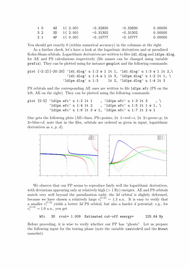
You should get exactly 0 (within numerical accuracy) in the columnn at the right.As a further check, let’s have a look at the logaritmic derivatives and at pseudized

Kohn-Sham orbitals. Logarithmic derivatives are written to files ld1.dlog and ld1ps.dlog,for AE and PS calculations respectively (file names can be changed using variableprefix). They can be plotted using for instance gnuplot and the following commands:

plot [-2:2][-20:20] ’ld1.dlog’ u 1:2 w l lt 1, ’ld1.dlog’ u 1:3 w l lt 2,\

’ld1.dlog’ u 1:4 w l lt 3, ’ld1ps.dlog’ u 1:2 lt 1, \

’ld1ps.dlog’ u 1:3 lt 2, ’ld1ps.dlog’ u 1:4 lt 3

PS orbitals and the corresponding AE ones are written to file ld1ps.wfc (PS on theleft, AE on the right). They can be plotted using the following commands:

plot [0:5] ’ld1ps.wfc’ u 1:2 lt 1 , ’ld1ps.wfc’ u 1:3 lt 3 , \

’ld1ps.wfc’ u 1:4 lt 2 , ’ld1ps.wfc’ u 1:5 lt 1 w l, \

’ld1ps.wfc’ u 1:6 lt 3 w l, ’ld1ps.wfc’ u 1:7 lt 2 w l

One gets the following plots (AE=lines, PS=points; lt 1=red=s; lt 2=green=p; lt3=blue=d; note that in the files, orbitals are ordered as given in input, logarithmicderivatives as s, p, d).

-20

-15

-10

-5

0

5

10

15

20

-2 -1.5 -1 -0.5 0 0.5 1 1.5 2

’ld1.dlog’ u 1:2’ld1.dlog’ u 1:3’ld1.dlog’ u 1:4

’ld1ps.dlog’ u 1:2’ld1ps.dlog’ u 1:3’ld1ps.dlog’ u 1:4

-0.4

-0.2

0

0.2

0.4

0.6

0.8

1

0 1 2 3 4 5

’ld1ps.wfc’ u 1:2’ld1ps.wfc’ u 1:3’ld1ps.wfc’ u 1:4’ld1ps.wfc’ u 1:5’ld1ps.wfc’ u 1:6’ld1ps.wfc’ u 1:7

We observe that our PP seems to reproduce fairly well the logarithmic derivatives,with deviations appearing only at relatively high (> 1 Ry) energies. AE and PS orbitalsmatch very well beyond the pseudization radii; the 3d orbital is slightly deformed,because we have chosen a relatively large r

(l=2)c = 1.3 a.u.. It is easy to verify that

a smaller r(l=2)c yields a better 3d PS orbital, but also a harder d potential: e.g., for

r(l=2)c = 1.0 a.u., you get

Wfc 3D rcut= 1.009 Estimated cut-off energy= 225.64 Ry

Before proceding, it is wise to verify whether our PP has “ghosts”. Let us preparethe following input for the testing phase (note the variable iswitch=2 and the &test

namelist):

&input


iswitch=2

/

&test

file_pseudo=’Ti.pbe-n-rrkj.UPF’,

nconf=1, configts(1)=’3d2 4s2 4p0’,

ecutmin=50, ecutmax=200, decut=50

/

This will solve the Kohn-Sham equation for the PP read from file pseudo, for a singlevalence configuration (nconf=1) listed in configts(1) (the ground state in this case),using a base of spherical waves whose cutoff (in Ry) ranges from ecutmin to ecutmax

in steps of decut. The initial part of the output looks good, but let us look at the testwith spherical waves, towards the end:

Cutoff (Ry) : 200.0

N = 1 N = 2 N = 3

E(L=0) = -0.7483 Ry -0.3282 Ry -0.0042 Ry

E(L=1) = -0.1077 Ry 0.0192 Ry 0.0630 Ry

E(L=2) = -0.2961 Ry 0.0304 Ry 0.0654 Ry

The lowest levels found in this way should be the same1 as those calculated from radialintegration (see above). This is true for the 4p state (-0.1077 Ry), for the 3d state(-0.2961 Ry vs -0.31302 Ry, see footnote), for the 4s state (-0.3282 Ry)....but note thespurious 4s level at -0.7483 Ry! Our PP has a ghost and is unusable.

What should be do now? we may try to change the definition of the local potential.We had chosen l = 1, let us try l = 2 and l = 0. The former has the same pathology,the latter has no ghosts. So our data for PP generation are as follows:

&input



iswitch=3

/

&inputp

pseudotype=1, nlcc=.true., lloc=0,

file_pseudopw=’Ti.pbe-n-rrkj.UPF’,

/

3

4P 2 1 0.00 0.00 2.9 2.9

3D 3 2 2.00 0.00 1.3 1.3

4S 1 0 2.00 0.00 2.9 2.9

(note lloc=0 and the 4s state at the end of the list). Let us plot again logarithmicderivatives and orbitals (they look quite the same as before) and run again the testwith spherical waves. We get (see the last section in the output):

1actually there are numerical differences, especially large for localized states like 3d, whose originis under investigation

Cutoff (Ry) : 50.0

N = 1 N = 2 N = 3

E(L=0) = -0.3282 Ry -0.0049 Ry 0.0361 Ry

E(L=1) = -0.1077 Ry 0.0192 Ry 0.0630 Ry

E(L=2) = -0.1469 Ry 0.0311 Ry 0.0682 Ry

Cutoff (Ry) : 100.0

N = 1 N = 2 N = 3

E(L=0) = -0.3282 Ry -0.0049 Ry 0.0361 Ry

E(L=1) = -0.1077 Ry 0.0192 Ry 0.0630 Ry

E(L=2) = -0.2959 Ry 0.0303 Ry 0.0652 Ry

Cutoff (Ry) : 150.0

N = 1 N = 2 N = 3

E(L=0) = -0.3282 Ry -0.0049 Ry 0.0361 Ry

E(L=1) = -0.1077 Ry 0.0192 Ry 0.0630 Ry

E(L=2) = -0.2961 Ry 0.0303 Ry 0.0652 Ry

This time the first column yields (with a small discrepancy for 3d) the expected levels,and only those levels. It is wise to inspect the second column as well for absenceof suspiciously low levels: ghosts may appear also as spurious excited states close tooccupied states. Note how bad the energy for the 3d level is at 50 Ry. At 100 Ryhowever we are close to convergence and at 150 Ry well converged, in agreement withthe estimate given during the PP generation (138 Ry).

We have now our first candidate (i.e. not surely wrong) PP. In order to 1) verifyif it really does the job, 2) quantify its transferability, 3) quantify its hardness, and 4)improve it, if possible, we need to perform some more testing.

3.1.2 Testing

As a first idea of how good our PP is, let us verify how it behaves on differente electronicconfiguration. The code allows to test several configurations in the following way:

&input


iswitch=2

/

&test

file_pseudo=’Ti.pbe-n-rrkj.UPF’,

nconf=9

configts(1)=’3d2 4s2 4p0’









/

here we have chosen 9 different valence configurations (the corresponding AE config-urations are obtained by superimposing configts to core states in config). Someof them are neutral, some are ionic, the first five leave the 3d states unchanged, thelast one is a completely ionized Ti4+. For each configuration, the code writes results(e.g. orbitals) into files ld1N.∗ and ld1psN.∗, where N is the index of the configura-tion. A summary is written to file ld1.test. For the first configuration, AE and PSeigenvalues and total energies are written:

3 2 3D 1( 2.00) -0.31302 -0.31302 0.00000

1 0 4S 1( 2.00) -0.32830 -0.32830 0.00000

2 1 4P 1( 0.00) -0.10777 -0.10777 0.00000

Etot = -1707.131006 Ry, -853.565503 Ha, -23226.698556 eV

Etotps = -9.748745 Ry, -4.874372 Ha, -132.638416 eV

(AE and PS eigenvalues are in this case the same, since this is the reference configura-tion used to build the PP). For the following configurations, AE and PS eigenvalues,plus total energy differences2 wrt configuration 1 are printed:

3 2 3D 1( 2.00) -0.40319 -0.40457 0.00138

1 0 4S 1( 1.00) -0.38394 -0.38420 0.00026

2 1 4P 1( 1.00) -0.15248 -0.15237 -0.00011

dEtot_ae = 0.226061 Ry

dEtot_ps = 0.226250 Ry, Delta E= -0.000189 Ry

The discrepancy between AE and PS energy differences (in this case, wrt the groundstate) as well as the discrepancies in AE and PS eigenvalues, are a measure of howtransferrable a PP is. In this case, the AE-PS discrepancy on δE = E(4s14p13d2) −E(4s24p03d2) (look at Delta E) is quite small, < 0.2 mRy, while the maximum dis-crepancy of the eigenvalues (rightmost column) ∼ 1 mRy. These are very good results.Unfortunately this is also a configuration that doesn’t differ much from the referenceone. Let us see the other cases:

3 2 3D 1( 2.00) -0.83550 -0.83256 -0.00295

1 0 4S 1( 1.00) -0.76075 -0.76163 0.00088

2 1 4P 1( 0.00) -0.48549 -0.48617 0.00068



3 2 3D 1( 2.00) -1.44648 -1.44538 -0.00110

1 0 4S 1( 0.00) -1.24186 -1.24652 0.00465

2 1 4P 1( 0.00) -0.91224 -0.91599 0.00375



2Reminder: absolute PS total energies depend upon the specific PP! Only energy differences aresignificant.

3 2 3D 1( 1.00) -0.68514 -0.74236 0.05722

1 0 4S 1( 2.00) -0.45729 -0.45802 0.00073

2 1 4P 1( 1.00) -0.18855 -0.18471 -0.00383



3 2 3D 1( 1.00) -1.16621 -1.21438 0.04817

1 0 4S 1( 2.00) -0.87720 -0.87620 -0.00100

2 1 4P 1( 0.00) -0.56807 -0.56137 -0.00670



3 2 3D 1( 1.00) -1.82248 -1.87471 0.05223

1 0 4S 1( 1.00) -1.39447 -1.39936 0.00489

2 1 4P 1( 0.00) -1.03942 -1.03465 -0.00476



3 2 3D 1( 1.00) -2.54976 -2.61959 0.06983

1 0 4S 1( 0.00) -1.94361 -1.96745 0.02383

2 1 4P 1( 0.00) -1.53584 -1.54419 0.00835



3 2 3D 1( 0.00) -3.84145 -3.95251 0.11106

1 0 4S 1( 0.00) -2.73793 -2.81405 0.07612

2 1 4P 1( 0.00) -2.25938 -2.28768 0.02831



It is evident that configurations with 3d2 occupancy are well reproduced, with errorson total energy differences < 3 mRy and on eigenvalues< 5 mRy. Configurations withdifferent 3d occupancy, however, have errors one order of magnitude higher. For theextreme case of Ti4+, the error is ∼ 0.1 Ry.

In order to better understand what is going on, let us have a look at the AE vs PSorbitals and logarithmic derivatives for configuration 9 (i.e. for the bare PP). Let usadd a line like this:


and plot files ld19ps.wfc, ld19.dlog, ld19ps.dlog using gnuplot as above :

-20

-15

-10

-5

0

5

10

15

20

-4 -3.5 -3 -2.5 -2 -1.5 -1 -0.5 0

’ld10.dlog’ u 1:2’ld10.dlog’ u 1:3’ld10.dlog’ u 1:4

’ld10ps.dlog’ u 1:2’ld10ps.dlog’ u 1:3’ld10ps.dlog’ u 1:4

-0.6

-0.4

-0.2

0

0.2

0.4

0.6

0.8

1

0 1 2 3 4 5

’ld10ps.wfc’ u 1:2’ld10ps.wfc’ u 1:3’ld10ps.wfc’ u 1:4’ld10ps.wfc’ u 1:5’ld10ps.wfc’ u 1:6’ld10ps.wfc’ u 1:7

Both the orbitals and the logarithmic derivatives (note the different energy range)start to exhibit some visible discrepancy now.

One can try to fiddle with all generation parameters, better if one at the time, tosee whether things improve. Curiously enough, the pseudization radius for the corecorrection, which in principle should be as small as possible, seems to improve thingsif pushed slightly outwards (try rcore=2.0). Also surprisingly, a smaller pseudizationradius for the 3d state, 0.9 or 1.0 a.u., doesn’t bring any visible improvement to trans-ferability (but it increases a lot the required cutoff!). Changing the pseudization radiifor 4s and 4p states doesn’t affect much the results.

A different local potential – a pseudized version of the total self-consistent potential– can be chosen by setting lloc=-1 and setting rcloc to the desired pseudization radius(a.u.). For small rcloc ghosts re-appear; rcloc=2.9 yields slighty better total energydifferences but slightly worse eigenvalues. Note that the PP so generated will also havea s projector, while the previous ones had only p and d projectors.

One could also generate the PP from a different electronic configuration. Since Titends to lose rather than to attract electrons, it will be more easily found in a ionizedstate than in the neutral one. One might for instance use the electronic configurationof the Bachelet-Hamann-Schluter paper[4]: 3d24s0.754p0.25. This however doesn’t seemto improve much.

Finally we end up with these generation data:

&input


iswitch=3

/

&inputp

pseudotype=1, nlcc=.true., rcore=2.0, lloc=0,

file_pseudopw=’Ti.pbe-n-rrkj.UPF’

/

3

4P 2 1 0.00 0.00 2.9 2.9

3D 3 2 2.00 0.00 1.3 1.3

4S 1 0 2.00 0.00 2.9 2.9

3.2 Single-projector, norm-conserving, with semicore states

The results of transferability tests suggest that a Ti PP with only 3d, 4s, 4p states havelimited transferability to cases with different 3d configurations. In order to improve it,a possible way is to put semicore 3s and 3p states in valence. The maximum for thosestates (0.87 a.u. and 0.90 a.u. respectively) is in the same range as for 3d (0.98 a.u.).Let us try thus the following:

&input



iswitch=3

/

&inputp

pseudotype=1, rho0=0.001, ...

file_pseudopw=’Ti.pbe-sp-rrkj.UPF’

/

3

3S 1 0 2.00 0.00 1.1 1.1

3P 2 1 6.00 0.00 1.2 1.2

3D 3 2 2.00 0.00 1.3 1.3

&test

configts(1)=’3s2 3p6 3d2 4s2 4p0’,

/

Note the presence of the &test namelist: it is used in this context to supply theelectronic valence configuration, to be used for unscreening. As a first step, we do notinclude the core correction. In place of the dots we should specify the local referencepotential. If we use lloc=-1 with large values of rcloc, (comparable to pseudizationradii for the previous case) we get all kinds of mysterious errors:

from compute_chi : error # 1

n is too large

for rcloc=2.5, while rcloc=2.7 produces an equally mysterious

from run_pseudo : error # 1

Errors in PS-KS equation

while smaller values (e.g. 1.5) lead to other errors:

WARNING! Expected number of nodes: 0 = 2-1-1, number of nodes found: 1.

Even if the code doesn’t stop, the presence of such messages is a signal of somethinggoing wrong in the generation algorithm. With some more experiments, though, onefinds that rcloc=1.3 yields a good potential. We still have other choices. In this case,d as reference potential: lloc=2, seems to work as well (and produces a PP with lessprojectors: only s and p). The generation algorithm in the latter case yields theseresults for Kohn-Sham energies:

n l nl e AE (Ry) e PS (Ry) De AE-PS (Ry)

1 0 3S 1( 2.00) -4.60347 -4.60348 0.00001

2 1 3P 1( 6.00) -2.85621 -2.85623 0.00002

3 2 3D 1( 2.00) -0.31302 -0.31301 -0.00001

2 0 4S 1( 2.00) -0.32830 -0.32892 0.00062

3 1 4P 1( 0.00) -0.10777 -0.10732 -0.00045

Note that the 3s, 3p, 3d levels should be the same by construction (the difference isnumerical noise); the 4s and 4p levels are not guaranteed to be the same. The factthat they are, to a very good degree, is very reassuring. A look at the orbitals willreveal that 3s, 3p, 3d are nodeless, 4s and 4p have one node. The spherical wave basisset confirms the absence of ghosts:

Cutoff (Ry) : 50.0

N = 1 N = 2 N = 3

E(L=0) = -4.5385 Ry -0.3263 Ry -0.0047 Ry

E(L=1) = -2.8427 Ry -0.1071 Ry 0.0193 Ry

E(L=2) = -0.1511 Ry 0.0311 Ry 0.0685 Ry

Cutoff (Ry) : 100.0

N = 1 N = 2 N = 3

E(L=0) = -4.5883 Ry -0.3279 Ry -0.0048 Ry

E(L=1) = -2.8547 Ry -0.1073 Ry 0.0193 Ry

E(L=2) = -0.2918 Ry 0.0303 Ry 0.0649 Ry

Cutoff (Ry) : 150.0

N = 1 N = 2 N = 3

E(L=0) = -4.5899 Ry -0.3280 Ry -0.0048 Ry

E(L=1) = -2.8549 Ry -0.1073 Ry 0.0193 Ry

E(L=2) = -0.2936 Ry 0.0303 Ry 0.0649 Ry

Note that for l = 0 the first (N = 1) level is the 3s level, the second (N = 2) levelis the 4s level, and the like for l = 1. Let us now repeat the testing on the nineselected configurations as for the 4-electron PP. You will have to add 3s2 3p6 to alltest configurations configts. Let us see check the errors on total energy differences:

$ grep Delta ld1.test




dEtot_ps = 0.343314 Ry, Delta E= 0.000077 Ry

dEtot_ps = 0.715061 Ry, Delta E= 0.001142 Ry




Energy differences are reproduced with an error that does not exceed a few mRy (seecolumn at the rhs). Eigenvalues are also well reproduced, e.g.:

1 0 3S 1( 2.00) -8.37382 -8.37230 -0.00152

2 1 3P 1( 6.00) -6.57173 -6.57195 0.00021

3 2 3D 1( 0.00) -3.84145 -3.83518 -0.00627

2 0 4S 1( 0.00) -2.73793 -2.74985 0.01192

3 1 4P 1( 0.00) -2.25938 -2.25525 -0.00412

although errors may reach 0.01 Ry (still one order of magnitude better than what weget with the previous 4-electron PP). The price to pay is the presence of more electronsin the valence.

3.3 Testing in molecules and solids

Even if our PP looks good (or not too bad) on paper based on the results of atomiccalculations, it is always a good idea to test it in simple molecular or solid-state systems,for which all-electron data (i.e. calculations performed with the same XC functionalbut without PP’s, such as e.g. FLAPW, LMTO, Quantum Chemistry calculations) isavailable. The comparison with experiments is of course interesting, but the goal ofPP’s is (at least in principle) to reproduce AE data, not to improve DFT.

A Atomic Calculations

A.1 Nonrelativistic case

Let us assume that the charge density n(r) and the potential V (r) are sphericallysymmetric. The Kohn-Sham (KS) equation:(

− ~2

2m∇2 + V (r)− ε

)ψ(r) = 0 (1)

can be written in spherical coordinates. We write the wavefunctions as

ψ(r) =

(Rnl(r)

r

)Ylm(r), (2)

where n is the main quantum number l = n − 1, n − 2, . . . , 0 is angular momentum,m = l, l − 1, . . . ,−l + 1,−l is the projection of the angular momentum on some axis.The radial KS equation becomes:(

− ~2

2m

1

r

d2Rnl(r)

dr2+ (V (r)− ε)1

rRnl(r)

)Ylm(r)

− ~2

2m

(1

sinθ

∂

∂θ

(sinθ

∂Ylm(r)

∂θ

)+

1

sin2θ

∂2Ylm(r)

∂φ2

)1

r3Rnl(r) = 0. (3)

This yields an angular equation for the spherical harmonics Ylm(r):

−(

1

sinθ

∂

∂θ

(sinθ

∂Ylm(r)

∂θ

)+

1

sin2θ

∂2Ylm(r)

∂φ2

)= l(l + 1)Ylm(r) (4)

and a radial equation for the radial part Rnl(r):

− ~2

2m

d2Rnl(r)

dr2+

(~2

2m

l(l + 1)

r2+ V (r)− ε

)Rnl(r) = 0. (5)

The charge density is given by

n(r) =∑nlm

Θnl

∣∣∣∣Rnl(r)

rYlm(r)

∣∣∣∣2 =∑nl

ΘnlR2nl(r)

4πr2(6)

where Θnl are the occupancies (Θnl ≤ 2l + 1) and it is assumed that the occupanciesof m are such as to yield a spherically symmetric charge density (which is true only forclosed shell atoms).

A.1.1 Useful formulae

Gradient in spherical coordinates (r, θ, φ):

∇ψ =

(∂ψ

∂r,1

r

∂ψ

∂θ,

1

rsinθ

∂ψ

∂φ

)(7)

Laplacian in spherical coordinates:

∇2ψ =1

r

∂2

∂r2(rψ) +

1

r2sinθ

∂

∂θ

(sinθ

∂ψ

∂θ

)+

1

r2sin2θ

∂2ψ

∂φ2(8)

A.2 Fully relativistic case

The relativistic KS equations are Dirac-like equations for a spinor with a “large” Rnlj(r)and a “small” Snlj(r) component:

c

(d

dr+κ

r

)Rnlj(r) =

(2mc2 − V (r) + ε

)Snlj(r) (9)

c

(d

dr− κ

r

)Snlj(r) = (V (r) + ε)Rnlj(r) (10)

where j is the total angular momentum (j = 1/2 if l = 0, j = l+1/2, l−1/2 otherwise);κ = −2(j − l)(j + 1/2) is the Dirac quantum number (κ = −1 is l = 0, κ = −l − 1, lotherwise); and the charge density is given by

n(r) =∑nlj

Θnlj

R2nlj(r) + S2

nlj(r)

4πr2. (11)

A.3 Scalar-relativistic case

The full relativistic KS equations is be transformed into an equation for the largecomponent only and averaged over spin-orbit components. In atomic units (Rydberg:~ = 1,m = 1/2, e2 = 2):

−d2Rnl(r)

dr2+

(l(l + 1)

r2+M(r) (V (r)− ε)

)Rnl(r)

− α2

4M(r)

dV (r)

dr

(dRnl(r)

dr+ 〈κ〉Rnl(r)

r

)= 0, (12)

where α = 1/137.036 is the fine-structure constant, 〈κ〉 = −1 is the degeneracy-weighted average value of the Dirac’s κ for the two spin-orbit-split levels, M(r) isdefined as

M(r) = 1− α2

4(V (r)− ε) . (13)

The charge density is defined as in the nonrelativistic case:

n(r) =∑nl

ΘnlR2nl(r)

4πr2. (14)

A.4 Numerical solution

The radial (scalar-relativistic) KS equation is integrated on a radial grid. It is conve-nient to have a denser grid close to the nucleus and a coarser one far away. Traditionallya logarithmic grid is used: ri = r0exp(i∆x). With this grid, one has∫ ∞

0

f(r)dr =

∫ ∞0

f(x)r(x)dx (15)

anddf(r)

dr=

1

r

df(x)

dx,

d2f(r)

dr2= − 1

r2df(x)

dx+

1

r2d2f(x)

dx2. (16)

We start with a given self-consistent potential V and a trial eigenvalue ε. The equationis integrated from r = 0 outwards to rt, the outermost classical (nonrelativistic forsimplicity) turning point, defined by l(l + 1)/r2t + (V (rt)− ε) = 0. In a logarithmicgrid (see above) the equation to solve becomes:

1

r2d2Rnl(x)

dx2=

1

r2dRnl(x)

dx+

(l(l + 1)

r2+M(r) (V (r)− ε)

)Rnl(r)

− α2

4M(r)

dV (r)

dr

(1

r

dRnl(x)

dx+ 〈κ〉Rnl(r)

r

). (17)

This determines d2Rnl(x)/dx2 which is used to determine dRnl(x)/dx which in turnis used to determine Rnl(r), using predictor-corrector or whatever classical integrationmethod. dV (r)/dr is evaluated numerically from any finite difference method. Theseries is started using the known (?) asymptotic behavior of Rnl(r) close to the nucleus(with ionic charge Z)

Rnl(r) ' rγ, γ =l√l2 − α2Z2 + (l + 1)

√(l + 1)2 − α2Z2

2l + 1. (18)

The number of nodes is counted. If there are too few (many) nodes, the trial eigenvalueis increased (decreased) and the procedure is restarted until the correct number n−l−1of nodes is reached. Then a second integration is started inward, starting from asuitably large r ∼ 10rt down to rt, using as a starting point the asymptotic behaviorof Rnl(r) at large r:

Rnl(r) ' e−k(r)r, k(r) =

√l(l + 1)

r2+ (V (r)− ε). (19)

The two pieces are continuously joined at rt and a correction to the trial eigenvalueis estimated using perturbation theory (see below). The procedure is iterated to self-consistency.

The perturbative estimate of correction to trial eigenvalues is described in the fol-lowing for the nonrelativistic case (it is not worth to make relativistic corrections ontop of a correction). The trial eigenvector Rnl(r) will have a cusp at rt if the trialeigenvalue is not a true eigenvalue:

A =dRnl(r

+t )

dr− dRnl(r

−t )

dr6= 0. (20)

Such discontinuity in the first derivative translates into a δ(rt) in the second derivative:

d2Rnl(r)

dr2=d2Rnl(r)

dr2+ Aδ(r − rt) (21)

where the tilde denotes the function obtained by matching the second derivatives inthe r < rt and r > rt regions. This means that we are actually solving a differentproblem in which V (r) is replaced by V (r) + ∆V (r), given by

∆V (r) = − ~2

2m

A

Rnl(rt)δ(r − rt). (22)

The energy difference between the solution to such fictitious potential and the solutionto the real potential can be estimated from perturbation theory:

∆εnl = −〈ψ|∆V |ψ〉 =~2

2mRnl(rt)A. (23)

B Equations for the Troullier-Martins method

We assume a pseudowavefunction Rps having the following form:

Rps(r) = rl+1ep(r) r ≤ rc (24)

Rps(r) = R(r) r ≥ rc (25)

wherep(r) = c0 + c2r

2 + c4r4 + c6r

6 + c8r8 + c10r

10 + c12r12. (26)

On this pseudowavefunction we impose the norm conservation condition:∫r<rc

(Rps(r))2dr =

∫r<rc

(R(r))2dr (27)

and continuity conditions on the wavefunction and its derivatives up to order four atthe matching point:

dnRps(rc)

drn=dnR(rc)

drn, n = 0, ..., 4 (28)

• Continuity of the wavefunction:

Rps(rc) = rl+1c ep(rc) = R(rc) (29)

p(rc) = logR(rc)

rl+1c

(30)

• Continuity of the first derivative of the wavefunction:

dRps(r)

dr= (l + 1)rlep(r) + rl+1ep(r)p′(r) =

l + 1

rRps(r) + p′(r)Rps(r) (31)

that is

p′(rc) =dR(rc)

dr

1

Rps(rc)− l + 1

rc. (32)

• Continuity of the second derivative of the wavefunction:

d2Rps(r)

d2r=

d

dr

((l + 1)rlep(r) + rl+1ep(r)p′(r)

)= l(l + 1)rl−1ep(r) + 2(l + 1)rlep(r)p′(r) + rl+1ep(r) [p′(r)]

2+ rl+1ep(r)p′′(r)

=

(l(l + 1)

r2+

2(l + 1)

rp′(r) + [p′(r)]

2+ p′′(r)

)rl+1ep(r). (33)

From the radial Schrodinger equation:

d2Rps(r)

dr2=

(l(l + 1)

r2+

2m

~2(V (r)− ε)

)Rps(r) (34)

that is

p′′(rc) =2m

~2(V (rc)− ε)− 2

l + 1

rcp′(rc)− [p′(rc)]

2(35)

• Continuity of the third and fourth derivatives of the wavefunction. This is assuredif the third and fourth derivatives of p(r) are continuous. By direct derivation of theexpression of p′′(r):

p′′′(rc) =2m

~2V ′(rc) + 2

l + 1

r2cp′(rc)− 2

l + 1

rcp′′(rc)− 2p′(rc)p

′′(rc) (36)

p′′′′(rc) =2m

~2V ′′(rc)− 4

l + 1

r3cp′(rc) + 4

l + 1

r2cp′′(r)

− 2l + 1

rcp′′′(rc)− 2 [p′′(rc)p

′′(rc)]2 − 2p′(rc)p

′′′(rc) (37)

The additional condition: V ′′(0) = 0 is imposed. The screened potential is

V (r) =~2

2m

(1

Rps(r)

d2Rps(r)

dr2− l(l + 1)

r2

)+ ε (38)

=~2

2m

(2l + 1

rp′(r) + [p(r)]2 + p′′(r)

)+ ε (39)

Keeping only lower-order terms in r:

V (r) ' ~2

2m

(2l + 1

r(2c2r + 4c4r

3) + 4c22r2 + 2c2 + 12c4r

2

)+ ε (40)

=~2

2m

(2c2(2l + 3) +

((2l + 5)c4 + c22

)r2)

+ ε. (41)

The additional constraint is:(2l + 5)c4 + c22 = 0. (42)

References

[1] D.R. Hamann, M. Schluter, and C. Chiang, Phys. Rev. Lett. 43, 1494 (1979).

[2] D. Vanderbilt, Phys. Rev. B 47, 10142 (1993).

[3] P. E. Blochl, Phys. Rev. B 50, 17953 (1994).

[4] G.B. Bachelet, D.R. Hamann and M. Schluter, Phys. Rev. B 26, 4199 (1982).

[5] X. Gonze, R. Stumpf, and M. Scheffler, Phys. Rev. B 44, 8503 (1991).

[6] S. Goedecker, M. Teter, and J. Hutter, Phys. Rev. B 54, 1703 (1996).

[7] N. Troullier and J.L. Martins, Phys. Rev. B 43, 1993 (1991).

[8] M.Fuchs and M. Scheffler, Comput. Phys. Commun. 119, 67 (1999).

[9] A. M. Rappe, K. M. Rabe, E. Kaxiras, and J. D. Joannopoulos, Phys. Rev. B 41,1227 (1990) (erratum: Phys. Rev. B 44, 13175 (1991)).

[10] L. Kleinman and D.M. Bylander, Phys. Rev. Lett. 48, 1425 (1982).

[11] S.G. Louie, S. Froyen, and M.L. Cohen, Phys. Rev. B 26, 1738 (1982).

[12] S.H. Wei and A. Zunger, Phys. Rev. B 37, 8958 (1987).

[13] First-principles norm-conserving pseudopotential with explicit incorporation ofsemicore states, Carlos L. Reis, J. M. Pacheco, and Jose Luıs Martins, Phys.Rev. B 68, 155111 (2003).

Notes on pseudopotential generation - Quantum...

Documents

Transcript of Notes on pseudopotential generation - Quantum...