NOTES ON MUMFORD-TATE GROUPS

(preliminary and incomplete version)

Centre Emile Borel

Paris, March 1999

by

Ben Moonen

§1. Hodge structures and their Mumford-Tate groups.

(1.1) Representations of algebraic tori. Let T be a torus over a field k. Choose a separable closure ks. Thecharacter group X∗(T ) and the cocharacter group X∗(T ) are defined by

X∗(T ) := Hom(Tks ,Gm,ks) , X∗(T ) := Hom(Gm,ks , Tks) .

If r is the rank of T then X∗(T ) and X∗(T ) are free abelian groups of rank r which come equipped with acontinuous action of Gal(ks/k). There is a natural perfect pairing X∗(T )×X∗(T ) −→ End(Gm,ks) = Z.

The functor

X∗( ):(algebraic tori

over k

)eq−→

(free abelian group of finite rank

+ continuous action of Gal(ks/k)

)

is an equivalence of categories. Similarly, the functor X∗( ) gives an anti-equivalence of categories.Let now ρ: T → GL(V ) be a representation of T on a finite dimensional k-vector space. If k = ks, so

that T ∼= Grm then the situation is clear: the space V decomposes as a direct sum of character spaces and this

completely determines the representation. Thus, a representation of Grm on a vector space V corresponds to

a Zr-grading

V =⊕

(n1,...,nr)∈Zr

V n1,...,nr .

Sign convention: we write V n1,...,nr for the subspace of V where (z1, . . . , zr) ∈ Grm acts as multiplication by

z−n11 · · · z−nr

r . (Note the minus signs.) This is nowadays the standard sign convention in Hodge theory, seefor instance [23], Remark 3.3.

Over an arbitrary field k, all we have to do is to require that the actions of Gal(ks/k) on X∗(T ) andon V ⊗k k

s “match”. Thus, let T be a k-torus and write Repk(T ) for the category of finite dimensionalk-representations of T . Then we have an equivalence of categories

Repk(T ) −→

finite dimensional k-vector spaces V +X∗(T )-grading V ⊗k k

s =⊕

χ∈X∗(T ) Vks(χ)

s.t. σ(Vks (χ)) = Vks(σχ) for all σ ∈ Gal(ks/k)

.

(1.2) The Deligne torus. Define the torus S by

S := ResC/R

Gm,C ,

where “Res” denotes restriction of scalars a la Weil. Thus, S is an algebraic torus over R; its character groupis generated by two characters z and z such that the induced maps on points

C∗ = S(R) ⊂ S(C) −→ Gm(C) = C∗

are the identity, resp. complex conjugation. In other words: X∗(S) = Z · z + Z · z with complex conjugationι ∈ Gal(C/R) acting by ιz = z, ιz = z. By what was explained in (1.1), this uniquely determines S as anR-torus.

Define the weight cocharacter w: Gm,R → S to be the cocharacter given on points by the naturalinclusion R∗ = Gm,R(R) → S(R) = C∗. The norm character Nm: S → Gm,R is defined by Nm = zz. Thekernel of Nm is the circle group U1 = z ∈ C∗ | |z| = 1, viewed as an R-torus. Finally we define thecocharacter µ: Gm,C → SC to be the unique cocharacter such that z µ is trivial and z µ = id ∈ End(Gm,C).

(1.3) Hodge structures. A Q-Hodge structure of weight n (n ∈ Z) consists of a finite dimensional Q-vectorspace V together with a homomorphism of algebraic groups over R

h: S→ GL(V )R

1

such that hw: Gm,R → GL(V )R is given by z 7→ z−n · idV . We leave it to the reader to connect this to themore traditional definition, using (1.1) above. By our sign convention, a point (z1, z2) ∈ C∗ × C∗ = S(C)acts on V p,q as multiplication by z−p

1 z−q2 .

We shall use HS as an abbreviation for “Hodge Structure”. By a Q-HS we shall mean a direct sum of pureQ-HS. Equivalently: a Q-HS is a finite dimensional Q-vector space V plus a homomorphism h: S→ GL(V )R

such that hw: Gm,R → GL(V )R is defined over Q. The category QHS of all such Q-HS is Tannakian.The automorphism C := h(i) of VR is called the Weil operator. Concretely: C acts on V p,q as multipli-

cation by iq−p. (Note that this indeed gives an endomorphism defined over R.)The Hodge filtration of V , notation F •VC, is the one given by FmVC = ⊕p≥mV

p,q. If V is pure of weightn then F •VC and F •VC are n-opposed in the sense of [16], meaning that F pVC ⊕ F qVC

∼−→ VC for all p, q

with p+ q = n+ 1. Conversely, if F •VC is a filtration of VC such that F •VC and F •VC are n-opposed thenwe obtain a HS by setting V p,q := F pVC ∩ F qVC.

The Tate structure Q(1) is defined to be the vector space Q(1) := 2πi · Q ⊂ C, with Hodge structurepurely of type (−1,−1). The corresponding homomorphism h is the Norm character Nm.

By a homomorphism of Hodge structures f : V1 → V2 we mean a Q-linear map f such that fR isequivariant w.r.t. the given actions of S. (This corresponds to a morphism of type (0, 0) in the traditionalsense, i.e., a map preserving the Hodge bigrading.)

A Q-HS V of weight n is said to be polarizable if there exists a homomorphism of Hodge structuresϕ: V ⊗ V → Q(−n) such that the bilinear form VR × VR → R given by (v, w) 7→ (2πi)n · ϕ(v ⊗ Cw) issymmetric and positive definite. This implies that ϕ is alternating if n is odd, symmetric if n is even. Anarbitrary Q-HS is said to be polarizable if all its pure summands are. We write QHSpol ⊂ QHS for the fullsubcategory of polarizable Q-HS.

(1.4) Definition. Let V be a Q-HS; write h: S→ GL(V )R for the corresponding homomorphism. We definethe Mumford-Tate group of V , notation MT(V ), to be the smallest algebraic subgroup M ⊆ GL(V ) (overQ) such that h factors through MR.

It is immediate from the definition that MT(V ) is connected. If V is pure of weight n 6= 0 then bylooking at hw we find that MT(V ) contains the torus Gm,Q · idV of homotheties. (By contrast, if V is pureof weight 0 then MT(V ) is contained in SL(V ); see also (1.11) below.)

It is easy to see that MT(V ) can also be described as the smallest algebraic subgroup M ⊂ GL(V ) suchthat hµ: Gm,C → GL(V )C factors through MC. This description will become important later.

(1.5) Key Property. Let V be a Q-HS. For m,n ∈ Z≥0, write Tm,n := V ⊗m ⊗ (V ∗)⊗n. Let T be a finitedirect sum of spaces of the form Tm,n, viewed as a Q-HS. Consider the action of MT(V ) on T induced byits action on V . Let W ⊆ T be a Q-subspace. Then

W ⊆ T is a Q-Hodge substructure ⇐⇒ W ⊆ T is a MT(V )-submodule .

Proof. The implication “⇐” is obvious. For “⇒”, suppose W is a Q-subHS. Consider the algebraicsubgroup M ⊆ GL(V ) consisting of those g ∈ GL(V ) which, under the induced action on T , leave thesubspace W ⊆ T stable. The assumption that W is a Q-subHS means that WR ⊂ TR is stable underthe (induced) action of S. It follows that h factors through M . The definition of MT(V ) then gives theimplication “⇒”.

If M ⊆ GL(V ) is an algebraic subgroup then there exists a “tensor construction” T as above and a linel ⊆ T such that M is the stabilizer of this line l. (Chevalley’s theorem, see e.g. [23], Prop. 3.1. Exercise:describe such a line for the case M = SL(V ) ⊂ GL(V ).) It follows that the Key Property characterizesMT(V ) uniquely.

(1.6) Definition. Let V be a Q-HS. A Hodge class in V is an element v ∈ V which is purely of type (0, 0)in the Hodge decomposition.

In other literature a Hodge class is sometimes defined to be a rational class which is purely of some type(p, p) in the Hodge decomposition. The connection between these two definitions is given by using a Tatetwist: if v ∈ V is a (p, p)-class then (2πi)p · v ∈ V (p) := V ⊗Q(1)⊗p is a Hodge class in our sense.

2

Exercise. Show that v ∈ V is a Hodge class if and only if v is invariant under MT(V ).

(1.7) Example. Suppose V is pure of weight n and ϕ: V ⊗ V → Q(n) is a polarization. Write ϕ ∈ (V ∗)⊗2

for the element given by (2πi)−n · ϕ. Then the line spanned by ϕ is stable under the action of MT(V ), whichmeans that MT(V ) acts on it through some character ν: MT(V )→ Gm,Q. The conclusion is that

MT(V ) ⊆

GSp(V, ϕ) if n is odd;GO(V, ϕ) if n is even.

Explanation: if V is a vector space over a field k equipped with a symplectic, resp. an orthogonal formϕ: V × V → k then we define the group of symplectic similitudes GSp(V, ϕ), resp. the group of orthogonalsimilitudes GO(V, ϕ), by

GSp(V, ϕ) := g ∈ GL(V ) | ∃ν(g) ∈ k∗ : ϕ(gv, gw) = ν(g) · ϕ(v, w) for all v, w ∈ V

and, similarly,

GO(V, ϕ) := g ∈ GL(V ) | ∃ν(g) ∈ k∗ : ϕ(gv, gw) = ν(g) · ϕ(v, w) for all v, w ∈ V .

Associating ν(g) to g gives a character ν: GSp(V, ϕ)→ Gm,k, resp. ν: GO(V, ϕ)→ Gm,k, called the multipliercharacter. The kernel of this multiplier character is the symplectic group Sp(V, ϕ), resp. the orthogonal groupO(V, ϕ).

If we want to treat the symplectic and the orthogonal case uniformly we shall write GU(V, ϕ) for thegroup of automorphisms of V preserving the form ϕ up to a scalar.

Exercise. Show that the multiplier character ν: MT(V )→ Gm,Q is independent of the chosen polarization.

(1.8) Remark. Let T be a tensor construction as in (1.5). Write r: GL(V ) → GL(T ) for the canonicalhomomorphism. Then MT(T ) equals the image of MT(V ) under r. To see this, let us first remark thatMT(T ) is contained in the image of MT(V ); this is immediate from the definitions. Now suppose thatMT(T ) is strictly contained in r(MT(V )). Then we can make a tensor construction T ′, built from T , anda Q-subspace W ⊂ T ′ such that W is a MT(T )-submodule but W is not stable under MT(V ). This wouldcontradict the Key Property. (Compare this with [25], Prop. 2.21.)

As examples of this principle, we find that MT(V ∗) is isomorphic to MT(V ) (under the natural isomor-phism g 7→ (g∗)−1). Also, MT(V ⊕n) (n ≥ 1) is isomorphic to MT(V ) acting diagonally on V ⊕n.

(1.9) Example. If dim(V ) = 0 then MT(V ) = 1. If dim(V ) = 1 then V is isomorphic to a Tate structureQ(n); if n = 0 then MT(V ) = 1, if n 6= 0 then MT(V ) = Gm,Q.

(1.10) Tannakian formulation. In the formalism of Tannakian categories, the Mumford-Tate group can bedescribed as follows. Let V be a Q-HS. Write 〈V 〉⊗ ⊂ QHS for the Tannakian subcategory generated byV . The forgetful functor defines a fibre functor ω: 〈V 〉⊗ → VecQ. Then MT(V ) = Aut⊗(ω) and we obtainan equivalence of categories 〈V 〉⊗

eq−→ RepQ(MT(V )). This is essentially just a fancy reformulation of the

above Key Property.

There are some possible variations on our definition of the Mumford-Tate group.

(1.11) Definition. Let V be a Q-HS of pure weight. We define the Hodge group Hg(V ) ⊆ MT(V ),also called the special Mumford-Tate group to be the smallest algebraic subgroup H ⊆ GL(V ) such thath|U1

: U1 → GL(V )R factors through HR.

If V has weight n and z ∈ S then the automorphism h(z) of V has determinant Nm(z)−n dim(V )/2.(Recall that h(z) is multiplication by z−pz−q on V p,q.) It follows that Hg(V ) is contained in SL(V ).

The relation between MT(V ) and Hg(V ) is not so difficult to describe. Namely, if V is pure of weight0 then we easily find that MT(V ) = Hg(V ). If V is pure of weight 6= 0 then MT(V ) contains Gm,Q (thehomotheties) and MT(V ) is the almost direct product (inside GL(V )) of Gm,Q and Hg(V ).

3

Now let us look at the key property (1.5). So, let T be a tensor space constructed from V and let W ⊆ Tbe a Q-subspace. Clearly, if W is a Q-subHS then it is a MT(V )-submodule, hence it is a Hg(V )-submodule.The converse holds provided T is of pure weight. This is clear if we think of MT(V ) as being the almostdirect product of Gm,Q and Hg(V ): the assumption that T is of pure weight means that Gm,Q acts on T byhomotheties, so that the MT(V )-submodules of V are the same as the Hg(V )-submodules. To summarize:

(1.12) Key Property. (Hodge group version.) Let V be a Q-HS. For m,n ∈ Z≥0, write Tm,n := V ⊗m ⊗(V ∗)⊗n. Let T be a finite direct sum of spaces of the form Tm,n, viewed as a Q-HS. Assume that T is ofpure weight. Consider the action of Hg(V ) on T induced by its action on V . Let W ⊆ T be a Q-subspace.Then

W ⊆ T is a Q-Hodge substructure ⇐⇒ W ⊆ T is a Hg(V )-submodule .

Loosely speaking we might say that Hg(V ) contains the same information as MT(V ), except that it isnot able to “see” the weight of a Hodge structure. For instance, if T is of pure weight and w ∈ T then wis a Hg(V )-invariant if and only if it is a Hodge (p, p)-class for some p. This also explains why we have torequire that T is of pure weight. Namely, suppose we can make two tensor spaces T1 and T2 and non-zeroclasses w1 ∈ T1 of type (p1, p1), and w2 ∈ T2 of type (p2, p2). Now set T := T1⊕T2, and let l ⊂ T be the linespanned by (w1, w2). Clearly, if p1 6= p2 then l is not a Q-subHS of T . But l is invariant under the actionof Hg(V ). That l is not stable under the action of MT(V ) is due to the action of the central torus Gm,Q.

(1.13) The Hodge group of a product. Let V1 and V2 be Q-HS. Write V := V1 ⊕ V2. It readily follows fromthe definitions that Hg(V ) ⊆ Hg(V1)×Hg(V2) and that the two projections Hg(V )→ Hg(Vi) are surjective.In general the Hodge group Hg(V ) need not be equal to the product group Hg(V1)×Hg(V2). For instance,if V1 = V2 then Hg(V ) is the diagonal subgroup of Hg(V1)×Hg(V2); see (1.8). We shall see more interestingexamples of this later.

For the Mumford-Tate group similar statements hold, but note that MT(V ) is almost never equal toMT(V1) ×MT(V2). This is because the central factor Gm (“keeping track of the weight”) is counted twicein MT(V1)×MT(V2), unless one of the Vi has weight 0.

(1.14) The extended Mumford-Tate group. Another possible variant is to consider the Tannakian subcate-gory 〈V,Q(1)〉⊗ ⊂ QHS generated by V and Q(1). Let ω: 〈V,Q(1)〉⊗ → VecQ be the forgetful functor, and

write MT(V ) := Aut⊗(ω). Concretely, this MT(V ) can be described as the smallest algebraic Q-subgroupM ⊂ GL(V ) × Gm,Q such that h × Nm: S → GL(V )R × Gm,R factors through MR. The projection onto

GL(V ) gives a surjective homomorphism MT(V )→→ MT(V ), which is an isogeny if V has weight n 6= 0 andan isomorphism if V is polarizable of weight ±1. See also [23] and [48].

One possible reason for working with this “extended” Mumford-Tate group MT(V ) is that it allows toinclude arbitrary Tate twists in all considerations. We leave it to the reader to formulate a version of theKey Property for MT(V ). (Consider tensor spaces of the form Tm,n,p := V ⊗m⊗ (V ∗)⊗n⊗Q(p).) Note thatMT(V ), for V polarizable of weight n, only has a natural action on Tate twists Q(r · n) for r ∈ Z. (Theaction on Q(−n) is given by the multiplier character ν as in (1.7).)

(1.15) Polarizable HS. Let V be a pure Q-HS of weight n, and let ϕ: V ⊗ V → Q(−n) be a polarization.Write Q: VR × VR → R for the symmetric positive definite form given by (v, w) 7→ (2πi)n · ϕ(v ⊗ Cw).

If T is a tensor space constructed from V as in (1.5) then T inherits a polarization from V . Similarly,if W ⊆ V is a Q-subHS then the restriction of ϕ to W ⊗ W is a polarization of W . Now consider theQ-subspace

W⊥ := x ∈ V | ϕ(x,w) = 0 for all w ∈ W .

Note that W⊥ is a Q-subHS of V ; writing V → V ∗(−n) for the morphism given by v 7→ ϕ(v,−) we can infact also define W⊥ as the kernel of the composite morphism V → V ∗(−n)→→ (V ∗/W ∗)(−n). As WR ⊂ VR

is stable under the Weil operator C, we have

(W⊥ ⊗ R) = x ∈ VR | ϕ(x,w) = 0 for all w ∈WR

= x ∈ VR | Q(x,w) = 0 for all w ∈WR .

4

It follows that V = W ⊕W⊥ as Q-HS.

(1.16) Theorem. The category QHSpol is a semi-simple Tannakian category. If V is a polarizable Q-HSthen Hg(V ) and MT(V ) are reductive Q-groups.

Proof. The first assertion follows from what was said in (1.15). The second claim is a general statementin the theory of Tannakian categories: if G is a connected group scheme over a field k of characteristic 0then Repk(G) is semi-simple if and only if G is pro-reductive. (See [25], Prop. 2.23.) In fact, in the casethat we are interested in it suffices to see that M := MT(V ) is reductive, as Hg(V ) is a normal subgroup ofMT(V ). We have RepQ(M)

eq−→ 〈V 〉⊗, which is semi-simple. In particular, the tautological representation

M → GL(V ) is faithful and semi-simple. It is then a standard result in the theory of algebraic groups (overa field of characteristic 0) that M is reductive. (Loc. cit., Lemmas 2.24, 2.25 and 2.27.)

Exercise. (i) Let V be a Q-vector space of finite dimension. Show that giving V a Q-HS of type (−1, 0) +(0,−1) is equivalent to giving an endomorphism C ∈ End(VR) (the Weil operator) with C2 = −id.

(ii) Let V be a polarizable Q-HS of weight n. Choose a polarization ϕ: V ⊗ V → Q(−n) and writed 7→ d† for the associated involution on D := EndQHS(V ). (So, d 7→ d† is the involution determined by therule that ϕ(dv ⊗ w) = ϕ(v ⊗ d†w) for all v, w ∈ V and d ∈ D.) Show that the set of polarizations is innatural bijection with an open cone in the vector space d ∈ D | d† = d.

(iii) Let V1 and V2 be polarizable Q-HS of type (−1, 0) + (0,−1). Write C1 ∈ End(V1,R) and C2 ∈End(V2,R) for the Weil operators. Suppose that EndQHS(V1) = Q = EndQHS(V2). Show that

ExtQHS(V2, V1) ∼= A ∈ Hom(V2,R, V1,R) | C1A+AC2 = 0/Q∗ .

(iv) Assume that V1 6∼= V2. Let W be an extension of V2 by V1 which corresponds to a non-zero class inExtQHS(V2, V1). (I.e., W 6∼= V1 ⊕ V2.) Show that W is not polarizable.

(v) Show that the category QHS is not semi-simple, e.g. by proving that there exist examples as in (iv).

(1.17) Compact real forms. Let V be a polarizable Q-HS of weight n. There is another way of provingthat H := Hg(V ) is reductive. (Although essentially it of course boils down to the same.) Namely, considerthe Weil operator C = h(i) ∈ H(R). As C2 = (−idV )n, the inner automorphism σ := Ad(C) of HR is aninvolution. Now consider the inner form H(σ) of H defined by this involution σ. Concretely: having a realgroup HR means that we have a complex group HC with a comlex conjugation x 7→ x. Then the inner formH(σ) is given by the same C-group HC but with x 7→ σ(x) as complex conjugation.

Let ϕ: V ⊗ V → Q(−n) be a polarization. Write Ψ: VC × VC → C for the symmetric, positive definitehermitian form (v, w) 7→ (2πi)nϕ(v ⊗ Cw). We claim that the real group H(σ) is a subgroup of the unitarygroup U(VC,Ψ) and is therefore compact. This is now a simple computation: let x ∈ H(σ)(R), so thatx = σ(x) = C−1xC. Then

Ψ(xv, xw) = (2πi)n · ϕ(xv ⊗ Cxw)

= (2πi)n · ϕ(xv ⊗ xCw) = (2πi)n · ϕ(v ⊗ Cw) = Ψ(v, w) .

This shows that HR is an inner form of a compact group. Now

H(σ) is compact =⇒ H(σ) is reductive⇐⇒ H(σ)C = HC is reductive⇐⇒ H is reductive .

(1.18) Remark. Let V be a polarizable Q-HS of weight n. From the fact that C ∈ Hg(V )(R) defines aCartan involution we can deduce some further conclusions. For this, decompose HR := Hg(V )R as HR =H0 · H1 · · ·Hq, the almost direct product of the connected center H0 and a number of R-simple factorsH1, . . . , Hq. Write pj : HR →→ H ′

j for the quotient of HR modulo H0 · · ·Hj−1 ·Hj+1 · · ·Hq and let Cj be theimage of C in H ′

j(R), which is again a Cartan involution.The first remark is that each of the factors Hj is absolutely simple. In fact, we have seen that the

Cartan involution σ = Ad(C) defines a compact inner form H(σ)j . Then the compactness of H

(σ)j implies

that Hj,C = H(σ)j,C is simple.

5

Further we conclude that:(i) the center of Hg(V ) is compact over R,(ii) if Hi(R) is not compact then h|U1

: U1 → Hg(V )R has a nontrivial component in the factor Hi,(iii) if Hi(R) is compact then C lies in the (finite) center of Hi.

In general it is not true that h|U1has a trivial component in the compact factors. For later use, let us

record here, however, that this is the case if V has level ≤ 1. By this we mean that either n is even andV is purely of type (n/2, n/2) or n = 2p + 1 is odd and V is of type (p, p + 1) + (p + 1, p); see also (2.22)below. So, we claim that if V has level ≤ 1 then h|U1

has a trivial component in the factor Hj if and only ifHj is compact. To see this, take a compact factor Hj and consider the action of U1 on Lie(H) ⊆ End(V ).The assumption that the level is ≤ 1 implies that in End(V ) only the Hodge types (−1, 1), (0, 0) and (1,−1)occur. Together with (iii) above it follows that Lie(Hj) ⊂ End(V )R is purely of type (0, 0). This means thatpj h|U1

factors through the finite center of H ′j , so the Hj-component of h|U1

is indeed trivial.

Exercise. Construct a polarizable Q-HS V such that Hg(V )(R) is compact. Also try to construct such anexample such that Hg(V ) is not a torus.

(1.19) Albert’s classification. Let D be a simple Q-algebra with a positive (anti-)involution ι: d 7→ d†. Suchalgebras have been classified by Albert; the result is explained in [53], §21. (What is a positive involution isalso explained for instance in [43], §2.) The result is that D is of one of the following types; here we writeF = Cent(D), F0 = a ∈ F | a† = a and e0 = [F0 : Q], e = [F : Q], d2 = [D : F ].

Type I(e0): e = e0, d = 1; D = F = F0 is a totally real field. The involution ι is the identity.

Type II(e0): e = e0, d = 2; D is a quaternion algebra over a totally real field F = F0; D splits at allinfinite places. The involution ι is different from the canonical involution on D (i.e., the onegiven by d 7→ d∗ = trD/F (d) − d); there exists an element a ∈ D with a∗ = −a such that

d† = ad∗a−1.

Type III(e0): e = e0, d = 2; D is a quaternion algebra over a totally real field F = F0; D is inert at allinfinite places. The involution ι is the canonical involution on D.

Type IV(e0, d): e = 2e0; F is a CM-field with totally real subfield F0; D is a division algebra of rank d2 overF . The involution ι is such that under a suitable isomorphism D ⊗Q R

∼−→ Md(C) × · · · ×

Md(C) (e0 factors) it coresponds to the involution (A1, . . . , Ae0) 7→ (A∗1, . . . , A

∗e0

), where

A∗i := tAi. In particular, ι is complex conjugation on F .

(1.20) Remark. As we have seen above, the category QHSpol of polarizable Q-HS is semi-simple. If V is asimple polarizable Q-HS then its endomorphism algebra D := EndQHS(V ) is a division algebra over Q. Letn be the weight of Q and let ϕ: V ⊗V → Q(−n) be a polarization. There is an involution d 7→ d† determinedby the rule ϕ(dv ⊗ w) = ϕ(v ⊗ d†w) for all v, w. By definition of a polarization, the form Q: VR × VR → R

given by Q(v, w) = (2πi)n ·ϕ(v⊗Cw) is symmetric and positive definite. Notice that d ∈ D commutes withthe Weil operator C, so that Q(dv, w) = Q(v, d†w). We conclude that d 7→ d† is a positive involution andthat D is an algebra of the type considered above.

(1.21) An upper bound for the Mumford-Tate group. Let V be a polarizable Q-HS. We can decompose Vas V = V m1

1 ⊕· · ·⊕Vmr

r , where V1, . . . , Vr are simple, mutually non-isomorphic Q-HS and m1, . . . ,mr ∈ Z≥1.Write D := EndQHS(V ), Di := EndQHS(Vi). The Di are division algebras of the type discussed above andD = Mm1(D1)× · · · ×Mmr

(Dr). If V is simple then we shall say it is of type I (type II, etc.) if D is of thecorresponding type in the Albert classification.

We haveD = EndQHS(V ) = Hodge classes in EndQ(V )

= MT(X)-invariants in EndQ(V )

= Hg(X)-invariants in EndQ(V ).

This means that MT(V ) is contained in the algebraic group GLD(V ) of D-linear automorphisms of V .Choosing a polarization ϕ of V and combining the previous with what we found in (1.7) we get

MT(V ) ⊆ GUD(V, ϕ) , Hg(X) ⊆ UD(V, ϕ) ,

6

where GUD(V, ϕ) and UD(V, ϕ) denote the centralizers of D inside GU(V, ϕ) resp. U(V, ϕ). Here we recallthat GU(V, ϕ) is our uniform notation for the group GSp(V, ϕ) (if V has odd weight, so that ϕ is symplectic),resp. GO(V, ϕ) (if V has even weight, so that ϕ is orthogonal).

Exercise. Show that this centralizer GUD(V, ϕ) does not depend on the chosen polarization.

(1.22) Classical groups. Let us make the group UD(V, ϕ) a little more explicit in the situation that D is afield. (In particular, V must be simple.) There are two cases to consider.

First suppose that D = F is a totally real field. Then there is a unique F -bilinear form ψ: V × V → Fwith the property that ϕ = trF/Q(ψ). We have an algebraic group UF (V, ψ) over F and the centralizerUF (V, ϕ) of F inside U(V, ϕ) is the group ResF/Q UF (V, ψ). We shall usually simply write UF (V, ψ) for thisgroup, assuming it is understood that we view it as an algebraic group over Q. If V has even weight then ψis symmetric and we have UF (V, ψ) = OF (V, ψ); if V has odd weight then UF (V, ψ) = SpF (V, ψ).

The other possibility is that D = F is a CM-field. Write F0 ⊂ F for its totally real subfield and x 7→ xfor the complex conjugation on F .

First assume that the weight of V is even, so that ϕ is symmetric. Then there exists a unique F -hermitian form ψ: V × V → F with ϕ = trF/Q(ψ). (So, ψ is F -linear in the first variable, F -anti-linear in

the second variable, and ψ(w, v) = ψ(v, w) for all v, w.) Now the unitary group UF (V, ψ) is an algebraicgroup over F0 and the centralizer SpF (V, ϕ) of F inside Sp(V, ϕ) is the group ResF0/Q UF (V, ψ). Again weshall usually simply write UF (V, ψ) for this group.

If the weight of V is odd then essentially the same works. Imitating the previous would lead us to workwith an anti-symmetric F -hermitian form ψ but we can modify this to a symmetric F -hermitian form usingan imaginary element in F . More precisely: choose an element a ∈ F with a = −a. Then there exists aunique F -hermitian form ψ: V × V → F with ϕ = trF/Q(a · ψ). Now again UF (V, ψ) is an algebraic groupover F0 and the centralizer SpF (V, ϕ) of F inside Sp(V, ϕ) is the group ResF0/Q UF (V, ψ).

If D is not a field the previous still works but has to be phrased in terms of D-hermitian forms. In eachcase we find that UD(V, ψ) is obtained by restriction of scalars from a classical group over the field F0. (Foralgebras with involutions, hermitian forms and algebraic groups, see for instance the appendix of [69], [9],section 23, or [41]).

(1.23) The center of the Mumford-Tate group. Let V be a polarizable Q-HS. Decompose V = V m11 ⊕ · · · ⊕

V mr

r as in (1.21). We have

D = [EndQ(V )]MT(V ) = [EndQ(V )]Hg(V ) . (1.23.1)

Write ZM = Z(MT(V )) for the connected center of the Mumford-Tate group. Then we see from (1.23.1)that ZM is contained in the algebraic group D∗ (viewed as an algebraic group over Q). Now again applying(1.23.1) we find that even ZM ⊆ TF := ResF/Q Gm, where F is the center of D.

By taking a polarization into account we can further sharpen this. First assume that V is simple, sayof weight n, and let d 7→ d† be the Rosati involution on D associated to a polarization ϕ: V ⊗ V → Q(−n).This involution induces complex conjugation on the center F . (The identity if F is totally real.) Write ZH

for the connected center of the Hodge group. If V has weight 0 then ZM = ZH ; otherwise ZM is isogenousto Gm,Q×ZH . The form ϕ is preserved by the Hodge group: we have ϕ(hv⊗hw) = ϕ(v⊗w) for all v, w ∈ Vand h ∈ Hg(V ). On the other hand, ϕ(dv ⊗ w) = ϕ(v ⊗ d†w) for d ∈ D. We conclude that ZH is containedin U0

F , where UF is the Q-group of multiplicative type given by

UF := x ∈ TF | xx = 1 .

On character groups TF and UF are described as follows: if ΣF is the set of embeddings F → Q thenX∗(TF ) is the free abelian group on ΣF , with its natural action of Gal(Q/Q). The character group X∗(UF )is the quotient of X∗(TF ) by the submodule generated by all elements σ+ σ, where the bar denotes complexconjugation.

Now drop the assumption that V is simple. In this case the center F is a product of totally real fieldsand CM-fields, say F = F1 × · · · × Fr. Set TF := TF1 × · · · × TFr

and UF := UF1 × · · · ×UFr. Using what

was said in (1.13) we again find that ZH is contained in U0F .

7

(1.24) Proposition. (See [88], Lemma 1.4.) Let V be a polarizable Q-HS. Assume V has no simple factorsof type IV. Then Hg(V ) is semi-simple.

Proof. This is clear from the previous, as the assumption implies that F is a product of totally realfields, so that UF is finite.

Next we look at the opposite extreme.

(1.25) Definition. A Q-HS is said to be of CM-type if V is polarizable and MT(V ) is a torus.

If V is of CM-type then Hg(V )(R) is compact, by (1.17). Conversely, if V is a Q-HS such that Hg(V )is a torus and Hg(V )(R) is compact then one can show that V is polarizable; see [70], Chap. 1, §6.1.

(1.26) Description of HS of CM-type. Let V be a polarizable Q-HS. Decompose V = V m11 ⊕ · · · ⊕ V mr

r asin (1.21). By what we have seen in (1.13), V is of CM-type if and only if each Vi is of CM-type.

Now assume that V is simple and of CM-type. Let F be the center of D := EndQHS(V ). Let d :=dimF (V ). In (1.23) we have seen that Hg(V ) ⊆ TF . This gives that Md(F ) ⊆ D. But D is a divisionalgebra, so d = 1 and for dimension reasons we then can only have D = F . By the Albert classification,either F is totally real or F is a CM-field.

If F is totally real then (1.23) gives Hg(V ) = 1. Then F = EndQ(V ) and we must have dim(V ) = 1and F = Q. We conclude that V ∼= Q(n) for some n. These are indeed of CM-type.

Next suppose F is a CM-field. If ϕ is a polarization of V then the associated Rosati involution onF is complex conjugation. We know that Hg(V ) ⊆ UF . For the Mumford-Tate group this means thatMT(V ) ⊆ GUF , where GUF ⊆ TF is the subtorus generated by UF and Gm,Q · id. On character groups:X∗(GUF ) is the quotient of X∗(TF ) (= the free abelian group on ΣF ) by the relations σ+ σ = τ + τ for allσ, τ ∈ ΣF . The homomorphism h: S→ GUF can now easily be described on character groups: it is given bya function

Φ: ΣF → Z2 , say σ 7→ (mσ, nσ)

such that (mσ, nσ) = (nσ,mσ) and such that the function σ 7→ mσ + nσ is constant (=the negative weight).Such a function Φ may be seen as a generalization of the classical notion of a CM-type (the case wheremσ, nσ ∈ 0, 1 for all σ, with weight equal to 1.) For the Hodge structure V this means the following. AsdimF (V ) = 1 we may identify V = F as an F -vector space. Then

V ⊗Q C∼−→

⊕

σ∈ΣF

C .

Then the summand C(σ) is of Hodge type (−mσ,−nσ). As C(σ) is the complex conjugate of C(σ), theconditions on the function Φ ensure that this indeed gives a Hodge structure on V , of weight mσ + nσ. Byconstruction this Hodge structure is simple and of CM-type.

(1.27) Question. (“Converse problem.”) Which algebraic groups can occur as the Hodge group of apolarizable Q-HS? In (1.16) and (1.18) we have found some conditions that such a group must satisfy;are these sufficient conditions? Although I have no complete answer, it seems to me that this question ismanageable. More interesting, and much more difficult is the question whether every “reasonable” groupoccurs as Hg(V ) for V a Q-HS “coming from geometry”. Here I have really no idea of what comes out. Forfurther discussion see for instance [35], [34] and [80]. Notice that there are many polarizable Q-HS which donot come from geometry; see [36], second footnote on page 300. (It would be very interesting to work outthis footnote in greater detail.)

(1.28) Remark. Let X be a smooth proper variety over C, say of dimension d. For 0 ≤ n ≤ 2d, letHgn(X) be the Hodge group of Hn(X,Q). Write Hg(X) for the Hodge group of H•(X,Q) := ⊕nH

n(X,Q).Then Hg(X) is a subgroup of

∏n Hgn(X), projecting surjectively to each factor (cf. (1.13)). In some cases,

for instance if X is an abelian variety, it is easy to describe the relation between Hg(X) and the Hgn(X).In general this is not so easy, but it helps to consider the decomposition of the cohomology into primitivepieces. There is a very natural generalization of this, which was proposed only recently in the paper [47]

8

by Looijenga and Lunts. The basic remark is this: the primitive decomposition depends on the choice ofan ample class in H2. It can be viewed as giving H•(X,Q) the structure of a module under sl2, wherethe primitive decomposition corresponds precisely to the decomposition of H•(X,Q) into irreducible sl2-representations. Now in general there is more than one ample class (up to multiples), and a different choicemay lead to a different primitive decomposition. Taking all, or several, ample classes in H2 simultaneously,one constructs a Lie algebra g (generally bigger than sl2) acting on H•(X,Q) and decomposing it into a sumof sub-Hodge structures. This decomposition can be finer than the usual primitive decomposition associatedto one ample class.

Further reading. There are many further ideas and constructions that we have not yet touched upon.Among them mixed Hodge structures, variation of Hodge structure, period domains, ... For those who wantto read more, Deligne’s papers [16], [17], [18], [19], [20], [21], [22] and [23] are a must. Other references ofgreat interest are (a fairly random selection): [25] and [68] (Tannakian categories), [14], [32], [33], [60], [86](variation of Hodge structure), [31] and [13] (overviews of various developments; the first more geometricallyoriented, the second more abstract), [2], [12], [61] (Mumford-Tate groups of mixed HS; in [2] we find a veryinteresting result on the relation with algebraic monodromy groups; the other two references deal with mixedShimura varieties). For papers containing interesting examples see also the suggestions at the end of thenext section.

§2. Mumford-Tate groups of abelian varieties.

(2.1) Abelian varieties. In this section we shall mainly look at Mumford-Tate groups of abelian varieties.There are several reasons why Mumford-Tate groups are particularly effective in this case. For one thing,if X is a complex abelian variety then H•(X,Q) ∼= ∧

•H1(X,Q) as Hodge structures, so that the wholecohomology of X , and even of all powers of X , is determined by H1(X,Q). Now H1(X,Q) is a polarizableHodge structure of level 1, by which we mean that hp,q = 0 if |p − q| > 1. As we shall see later, thisputs interesting restrictions on MT(V ). In the sequel, if X is a complex abelian variety we shall writeMT(X) := MT(H1(X,Q)) and Hg(X) := Hg(H1(X,Q)).

Another thing that is special about abelian varieties is that we have a very strong “Torelli” result:

(2.2) Theorem. The functor X 7→ H1(X,Z) gives an equivalence of categories

(abelian varieties

over C

)eq.−→

(polarizable torsion-free Z-HS

of type (−1, 0) + (0,−1)

).

As variants of this equivalence: polarized abelian varieties correspond to polarized HS, abelian varietiesup to isogeny correspond to polarizable Q-HS of type (−1, 0) + (0,−1), and families of abelian varietiescorrespond to polarizable variations of Hodge structures.

Notice that the duality X 7→ Xt := Pic0X/C of abelian varieties corresponds to the duality V 7→ V ∗(1)

of Hodge structures. Furthermore, the notions of a polarization correspond: if λ: X → Xt is a polarizationof the abelian variety X then the induced morphism ϕ = H1(λ): H1(X,Z)→ H1(X,Z)∗(1) is a polarizationof the Hodge structure H1(X,Z) and vice versa. The form (2πi)−1 · ϕ is usually referred to as the Riemannform of the polarization.

(2.3) The results of §1 for V = VX . Let X be a complex abelian variety. A first consequence of (2.2)—andthis is really special about abelian varieties—is that the endomorphism algebra ofX equals the endomorphismalgebra of VX :

End0(X)∼−→ EndQHS(VX) ,

9

where we set End0(X) := End(X) ⊗Z Q. (That D := End0(X) is a semi-simple Q-algebra with a positiveinvolution is in fact true over an arbitrary field. Given g := dim(X), there are some numerical restrictionson what D can be. See [53], §21, [59], [81].)

Up to isogeny (notation ∼) we can decompose X as

X ∼ Y m11 × · · · × Y mr

r ,

where Y1, . . . , Yr are simple, mutually non-isogenous, abelian varieties and m1, . . . ,mr ∈ Z≥1. Write Vi :=H1(Yi,Q) and Di := End0(Yi). Then VX = V m1

1 ⊕ · · · ⊕ V mr

r is a decomposition of VX as a direct sum ofsimple Q-HS and D = Mm1(D1)× · · · ×Mmr

(Dr). If r = 1 then we say that X is elementary. If X is simple(i.e., r = 1 and m1 = 1) then we say that X is of type I (type II, etc.) if D is of the corresponding type inthe Albert classsification.

Let λ: X → Xt be a polarization of X . As explained above, it corresponds to a polarization ϕ: VX ⊗VX → Q(−1) of VX . In (1.21) we have seen that

MT(X) ⊆ GSpD(VX , ϕ) , and D = [End(VX)]MT(X) .

From the description given in (1.26) we easily see that X is of CM-type (in the sense of abelian varieties) ifand only if VX is of CM-type, i.e., iff MT(X) is a torus. This was first proven by Mumford, [52]. If X hasno simple factors of type IV then Hg(X) is semi-simple.

(2.4) Let X be a simple abelian variety over C. Set g := dim(X). As remarked above, there are somenumerical restrictions on what D := End0(X) can be. Most of these can be derived by remarking thatV := H1(X,Q) is a 2g-dimensional Q-vector space on which D acts and such that there exists a symplecticform ϕ with ϕ(dv, w) = ϕ(v, d†w) for all v, w,∈ V and d ∈ D. Writing e := [F : Q] and d2 := [D : F ] wefind that e|g if X has type I, that 2e|g if X has type II or III and that ed2|2g if X has type IV.

There are some further invariants associated to the action of D on V . The ones we shall need can bedescribed as follows. Write ΣF for the set of embeddings of F into C. Then V ⊗Q C = V −1,0 ⊕V 0,−1 is freeof rank 2g/e over

F ⊗Q C =∏

σ∈ΣF

C .

Moreover, the action of F ⊗Q C respects the Hodge decomposition of VC. Therefore we can write

V ⊗Q C =⊕

σ∈ΣF

V −1,0(σ)⊕ V 0,−1(σ) ,

where V i,j(σ) = v ∈ V i,j | f(v) = σ(f) · v for all f ∈ F. We shall write

nσ := dimC V−1,0(σ) .

Note that dim V −1,0(σ)+dim V 0,−1(σ) = 2g/e for all σ. Also, writing σ for the complex conjugate of σ, thesummand V −1,0(σ) is complex conjugate to V 0,−1(σ). This gives the relation

nσ + nσ = 2g/e for all σ ∈ ΣF .

The integers nσ are often referred to as the multiplicities of the action of F on the tangent space of X ; noticethat V −1,0 is indeed naturally isomorphic to the tangent space of X at the origin.

(2.5) Comment. How succesful we are in describing, or computing, the Mumford-Tate group of an abelianvariety strongly depends on how we play the game. By this we mean the following. If we take an “abstract”abelian variety, we can decompose it (up to isogeny) as a product of powers of simple ones. Then, using theAlbert classification, we find a finite list of possibilities for the endomorphism algebra. In each of the possiblecases we can try to determine the Mumford-Tate group, possibly after taking into account further “discrete”invariants, such as the type of the action on the tangent space. In many cases this leads to interesting results,

10

and we shall see that sometimes it even allows to prove the Hodge conjecture for our abelian variety. Usually,however, the abelian variety itself remains “invisible” in this game; it is not a concrete geometric object.What we are really studying are abstract Q-Hodge structures satisfying certain properties. By contrast, ifwe start with an abelian variety as coming from some geometric situation, e.g., as the Jacobian of someother variety, then it is often very hard to determine its Mumford-Tate group.

(2.6) Example. Let E be an elliptic curve over C. We know that the Hodge group Hg(E) is a reductivesubgroup of Sp(V, ϕ) = SL2,Q. A priori there are therefore only three possibilities: either (a) Hg(E) = 1,or (b) Hg(E) = SL2,Q, or (c) Hg(E) is a maximal torus of SL2,Q. On the other hand, we know that eitherEnd0(E) = Q or End0(E) = k is an imaginary quadratic field. This rules out case (a). The remainingoptions are now easily matched:(i) if End0(E) = Q then Hg(E) is semi-simple so we must have Hg(E) = SL2,Q.(ii) if End0(E) = k is an imaginary quadratic field then Hg(E) is a torus contained in Uk = z ∈ k∗ | zz = 1;

see (1.23). Since Uk has rank 1 we have Hg(E) = Uk.

(2.7) Example. Let X be a simple abelian surface. For D := End0(X) we have the following four possi-bilities:(i) D = Q,(ii) D = F is a real quadratic field,(iii) D is an indefinite quaternion algebra over Q,(iv) D = F is a CM-field of degree 4 over Q which does not contain an imaginary quadratic field.(Note that for dim(X) = 2 we cannot have that End0(X) is an imaginary quadratic field; see [81].)

We claim that in each of these cases we have Hg(X) = SpD(V, ϕ). We first do case (ii). We know thatHg(X) is semi-simple and contained in SpF (V, ψ) = SLF (V ) ∼= ResF/Q SL2,F . Write H for this group. Then

HC∼= SL2 × SL2. Writing St(1) resp. St(2) for the standard respresentation of the first (resp. second) factor

SL2 we have VX ⊗Q C ∼= St(1) ⊕ St(2) as a HC-module. Now assume that Hg(X) 6= SpF (V, ϕ). As Hg(X) issemi-simple we must have Hg(X)C

∼= SL2 −→ HC = SL2 × SL2. Since

End(VX,C)Hg(X)C = [End(VX)Hg(X)]⊗ C = F ⊗ C ∼= C× C (2.7.1)

the projections of Hg(X)C to the two factors SL2 are both surjective. Now remark that SL2 has only oneirreducible 2-dimensional representation, up to isomorphism. It follows that VX,C

∼= St⊕2 as a representationof Hg(V )C. As this contradicts (2.7.1) we conclude that Hg(X) = SpF (V, ψ) = SLF (V ).

Case (iii) is quite easy. We know that Hg(X) is semi-simple and contained in SpD(V, ϕ). The lattergroup can be described as follows. Let Dopp be the opposite of the algebra D and write d 7→ d∗ for itscanonical involution. Then SpD(V, ϕ) ∼= UDopp , the algebraic Q-group given on points by

UDopp = d ∈ (Dopp)∗ | dd∗ = 1 ,

which is a Q-form of SL2. By rank considerations we must have Hg(X) = UDopp .Case (iv) is also not difficult. In this case Hg(X) is contained in the torus UF , which has rank 2. Using

that F does not contain an imaginary quadratic field, one checks that UF does not contain any nontrivialQ-subtorus. (This is done using the explicit description of X∗(UF ) given in (1.23).)

Finally, suppose we are in case (i). Then Hg(X) is semi-simple, contained in SpQ(V, ϕ) ∼= Sp4,Q, andVX,C is an irreducible representation of Hg(X)C. Suppose that Hg(X) 6= Sp(V, ϕ). By rank considerationswe must have Hg(X)C

∼= SL2 and VX,C∼= Sym3(St). (Notice that SL2 × SL2 does not have an irreducible

faithful symplectic representation of dimension 4. Also notice that −id ∈ Z(Hg), so Hg(X)C could also notbe PSL2.) If T ⊂ Hg(X)C is a maximal torus and t is a generator of the character group X∗(T ) then theweights of T that occur are

t−3 t−1 t t3

• • • •

Let T ⊂ MT(X)C be the maximal torus generated by Gm · id and T . (We are still assuming that Hg(X)C∼=

SL2.) Then X∗(T ) ∼= Z2 and the 4 weights of T on VX,C lie on a line (not through the origin). At this

11

point we use a little extra information about the Hodge structure VX,C. Namely, consider the cocharacterhµ: Gm,C → MT(X)C. Letting Gm act on VX,C through this cocharacter we know that the weights that

occur are z 7→ z−1 and z 7→ 1. We can choose our T such that hµ factors through it. On character groupsthis gives a Z-linear map X∗(T ) → X∗(Gm) = Z such that the 4 weights of T map onto the 2 weights ofGm. This is clearly impossible. We conclude that Hg(X) = Sp(V, ϕ).

(2.8) Remark. Let X be a complex abelian variety. Let T ⊂ MT(X)C be a maximal torus. Assume thatEnd0(X) = Q, which means precisely that VX,C is an irreducible representation of MT(X)C. The weights of

T in VX,C form a finite subset (with multiplicities) Supp(VX,C) ⊂ X∗(T ) ∼= Zr. The arguments used in case

(i) above can be visualized by saying that there exists a Z-linear map X∗(T ) → Z such that the image ofSupp(VX,C) consists of two elements. In other words: the weights that occur lie in two parallel hyperplanes

inside X∗(T ). This restriction comes from the fact that only two types occur in the Hodge decompositionof VX and puts strong restrictions on the representations that can occur. Similar arguments can be appliedto arbitrary Hodge structures; we shall study this in §3.

(2.9) The Hodge conjecture. We shall use Mumford-Tate groups to prove the Hodge conjecture in certaincases. Let us first set up some notations and recall the statement of the conjecture.

Let X be a nonsingular proper variety over C. We write Bn(X) ⊆ H2n(X,Q)(n) for the subspace ofHodge classes. Then B

• := ⊕nBn(X) is a commutative graded Q-algebra, called the Hodge ring of X . If Zis an algebraic cycle on X of codimension n then there is an associated cohomology class cl(Z) ∈ Bn(X). Wein fact have a homomorphism of graded Q-algebras cl : CH

•

Q(X)→ B•(X). The (special) Hodge conjecture

is the following:HC(X,n) : the map cl : CHn

Q(X)→ Bn(X) is surjective.

In other words, the conjecture says that every Hodge class in H2n(X,Q)(n) is a Q-linear combination ofalgberaic classes cl(Z). Let us also write HC(X) for the statement “HC(X,n) holds for all n”.

Although the Hodge theorem (which gives rise to the Hodge structure on H2n(X,Q)) works for compactKahler manifolds, not necessarily projective, it is known that the Hodge conjecture is definitely false forgeneral compact Kahler manifolds. For an example, see [46], ??.

The Hodge conjecture was originally formulated by Hodge with Z-coefficients. In the paper [5] byAtiyah and Hirzebruch it was shown however, that H2n(X,Z)(n) may contain torsion classes which are notalgebraic. But not only torsion phenomena force us to work with Q-coefficients: it may also happen thatH2n(X,Z)(n) contains elements ξ which are not torsion, such that some multiple m · ξ is the class of analgebraic cycle but ξ itself is not; see for instance [6].

(2.10) Divisor classes. It is a theorem of Lefschetz that HC(X, 1) holds for every (proper, nonsingular)X . So, B1(X) ⊂ H2(X,Q)(1) is generated by the divisor classes. Now set D1(X) := B1(X), and writeD

•(X) ⊆ B•(X) for the Q-subalgebra generated by D1(X). In other words: D

•(X) consists of all Q-linearcombinations of cup-products of divisor classes. Clearly all classes in D

•(X) are algebraic; in particular, ifD

•(X) = B•(X) then the Hodge conjecture is true for X .

In general it is quite easy to cook up examples where D•(X) 6= B

•(X), taking X to be a (suitable)hypersurface in some Pn for instance. For abelian varieties the situation is different. We shall find manycases where D

•(X) = B•(X), and it is not so easy to produce examples where this actually does not hold.

We shall further go into this below.

(2.11) The basic strategy. Let us now explain a strategy that was already hinted at in (2.5). Take anabelian variety X . We want to prove HC(X), or at least we want to find out if D

•(X) = B•(X).

Assume we know D := End0(X). In any case, knowing X , and possibly the way X decomposes intosimple factors, the Albert classification gives us a finite number of possible “types” for D, which we can tryto deal with one by one. Now we have

MT(X) ⊆ GSpD(V, ϕ) , and D = [End(VX)]MT(X) .

The first gives an “upper bound” for MT(X), the second says that MT(X) cannot be too much smaller

12

than GSpD(V, ϕ). Using this, combined with various facts from the theory of reductive groups, we can tryto determine (a finite list of possibilities for) MT(X) and its representation VX .

Once we know (a candidate for) MT(X) we can turn things around: the Hodge ring B•(X) is the space

of Hg(X)-invariants in ∧•VX , and is therefore (at least in principle) easy to compute. (Note that for thecomputation of invariants we can extend scalars to C, which is sometimes helpful.) In any case, the questionwhether D

•(X) = B•(X) now becomes a problem in invariant theory.

(2.12) Some results from invariant theory. Almost all we shall need from invariant theory can be reducedto one of the following cases.

(C) Symplectic groups. Let W be a C-vector space equipped with a non-degenerate symplectic form ϕ.Let m ∈ Z≥1. Then the graded C-algebra

[

•∧(W⊕m)]Sp(W,ϕ)

is generated by its elements in degree 2.(A) Unitary groups. Let W be a C-vector space equipped with a non-degenerate hermitian form ϕ. Let

m ∈ Z≥1. Then the graded C-algebra

[

•∧(W⊕m)]U(W,ϕ)

is generated by its elements in degree 2.

(2.13) Example. Suppose X is simple and End0(X) = F is a totally real field. Suppose furthermore thatMT(X) = GSpF (V, ϕ), so Hg(X) = SpF (V, ϕ). Let ΣF = σ1, . . . , σe be the set of embeddings of F intoC and set d = dimF (VX). Then VX,C is free of rank d over F ⊗Q C = C(1) × · · · × C(e), so it decomposesas VX,C = W(1) ⊕ · · · ⊕W(e). The symplectic form ϕ on VX,C decomposes as a sum of symplectic formsϕ(j): W(j) ×W(j) → C(j). (Exercise: show this, using that the Rosati involution on F is trivial.) We thenhave SpF (VX , ϕ)⊗ C = Sp(W(1), ϕ(1))× · · · × Sp(W(e), ϕ(e)) and

B•(Xm) = [

•∧(V ⊕m

X,C )]SpF

(VX ,ϕ)⊗C = [

•∧(W⊕m

(1) )]Sp(W(1),ϕ(1)) ⊗ · · · ⊗ [

•∧(W⊕m

(e) )]Sp(W(e),ϕ(e)) .

Applying (2.12), case (C), we find that this algebra is generated by its elements in degree 2, which justmeans that D

•(Xm) = B•(Xm) for all m.

Similar arguments, now working with unitary groups, work in case F is a CM-field and Hg(X) =UF (VX , ϕ).

Let us now give a number of results on Mumford-Tate groups of abelian varieties and applications tothe Hodge conjecture. For the proofs of these results we refer to the literature. First we have a result ofHazama [37] and Murty [54]. The proof heavily uses invariant theory of the kind indicated above.

(2.14) Theorem. Let X be a complex abelian variety. Set D := End0(X), let V := H1(X,Q) and let ϕ bethe Riemann form of a polarization. Then

B•(Xn) = D

•(Xn) for all n ≥ 1 ⇐⇒

(X has no factors of type IIIand Hg(X) = SpD(V, ϕ)

).

The next result, and especially its corollary, is perhaps surprising if you see it for the first time. Afterall, a priori most people would probably not expect simple abelian varieties of dimension 31, say, to be muchsimpler than ones of dimension 32, say. But if we think of abelian varieties (up to isogeny) just as beingspecial kinds of Hodge structures then it is already much more plausible that numerical conditions on thedimension could make a big difference for what possibilities may occur.

The corollary is due to Tankeev [89], although it seems that several cases were done independently byRibet and Serre. The theorem as we state it includes generalizations due to Ribet [67]. We refer to this very

13

readable paper for the proof. Some of the technical results needed in the paper are discussed in the nextsection. (See for instance (3.14) where we prove a special case of statement (i).) In the statement we usethe notations as explained in (1.22) and (2.4).

(2.15) Theorem. Let X be a complex abelian variety. Set g := dim(X).(i) Suppose End0(X) = F is a totally real field such that the integer g/[F : Q] is odd. Then Hg(X) =

SpF (V, ψ).(ii) Suppose End0(X) = k is an imaginary quadratic field such that nσ and nσ are relatively prime.

Then Hg(X) = Uk(V, ψ).(iii) Suppose g is prime and End0(X) = F is a CM-field of degree 2g over Q. Then Hg(X) = UF (V, ψ) =

UF .

(2.16) Corollary. Let X be a simple abelian variety of prime dimension. Then Hg(X) = SpD(V, ϕ)(notations as in (2.14)) and B

•(Xn) = D•(Xn) for all n. In particular, the Hodge conjecture is true for all

Xn.

To get the corollary from the theorem note that if X is simple of prime dimension g, the endomorphismalgebra End0(X) can only be Q, or a totally real field of degree g over Q, or an imaginary quadratic field,or a CM-field of degree 2g over Q. All these cases are covered by (2.15). Note also that X is not of type III,so that (2.14) applies. (In fact, in all cases that occur the implication “⇐” in (2.14) can be proven by hand;(2.14) in its full strength was proven later than (2.15) and (2.16).)

There are many more cases where it is proven that Hg(X) = SpD(V, ϕ); see for instance [38], [50], [49],[55], [62] or the many references given in [30].

(2.17) Weil classes. Let us now explain a construction that leads to examples where B•(X) 6= D

•(X). Thefirst such example (with X an abelian variety) was given by Mumford; see [64]. The construction given hereis due to Weil [94], who remarked that there is one ingredient in the example constructed by Mumford whichis essential. For more details we refer to [51].

Start with a Q-HS V , a (commutative) field k and a homomorphism k → EndQHS(V ) sending 1 to idV .Set d := dimk(V ). Then ∧d

kV is a 1-dimensional k-vector space and there is a canonical Q-linear surjection

p = pV :d∧

Q

V →→d∧

k

V .

It is not difficult to show that Ker(p) is a Q-subHS of ∧dQV . By the semi-simplicity of QHS is follows that

there is a unique Q-subHS

Wk ⊂

d∧

Q

V

which maps isomorphically to ∧dkV under p. Alternatively, as we are working over a ground field of charac-

teristic 0 the natural Q-linear map (∧dQV )∗ → [∧d

Q(V ∗)] is an isomorphism and we may define Wk ⊂ ∧dQV

by dualizing pV ∗ . We refer to Wk as the space of Weil classes w.r.t. the given action of k.Let us now specialize this to the case of abelian varieties, taking V = H1(X,Q). In this case Wk is a

subspace of Hd(X,Q) and one can show ([51], sections 2–6) that the following conditions are equivalent:(i) the space Wk contains a non-zero Hodge class,(ii) the space Wk consists entirely of Hodge classes,(iii) for all embeddings σ: k → C we have, using the notations introduced in (2.4), nσ = nσ,(iv) the Hodge group Hg(X) ⊂ GLk(V ) is contained in SLk(V ).

For instance, if X has no factors of type IV then Hg(X) is semi-simple and (iv) is automatically satisfied.Notice that the four equivalent conditions can only be satisfied if V has even dimension as a k-vector space.

Now suppose that Wk consists of Hodge classes. Then the next question is whether these classes lie inD

•(X). In loc. cit. we find a complete answer to this questions, purely in terms of the given action of k onX . Here we shall only give some examples.

14

Exercise. The multiplicative group k∗ acts on V . It also acts on Wk. Describe how the two actions arerelated. Show that (i) and (ii) above are equivalent. Also show that if there is one non-zero class in Wk

which lies in D•(X) then Wk is fully contained in D

•(X).

(2.18) Example. Suppose that X is simple and that End0(X) = k is an imaginary quadratic field. Thisimplies that X has even dimension, say dim(X) = 2d. Suppose furthermore that the multiplicities of theaction of k on the tangent space of X at the origin satisfy nσ = nσ = 2d. Then Wk ⊂ H2d(X,Q) is a2-dimensional subspace consisting of Hodge classes. But the Picard number of X (:= the dimension ofB1(X)) is 1. So Wk could impossibly be contained in Dd(X). ˚e conclude that Wk consists of exceptionalHodge classes, i.e., Hodge classes which do not lie in D

•(X).

(2.19) Example. Suppose that X is simple of type III. Recall that this means that D := End0(X) is aquaternion algebra over a totally real field F such that D is inert at all infinite places. Notice that for everyelement α ∈ D \ F the subfield F (α) ⊂ D is a CM-field. Take k = F (α) for such an α. As remarked above,the semi-simplicity of Hg(X) implies that Wk consists of Hodge classes. In fact, with a construction as in(1.22) we find that the Hodge group is contained in a special unitary group SUk(V, ψ). Next one showsthat all divisor classes are invariant under the full unitary group Uk(V, ψ) and that this group acts on Wk

as multiplication by the k-linear determinant detk: Uk(V, ψ) → k∗. Again it follows that Wk consists ofexceptional Hodge classes. (For more details see e.g., [50], especially section 3.)

(2.20) Example. As a final example, suppose that X is a product of two abelian varieties, say X = Y1×Y2.Set di := 2 dim(Yi)/[k : Q], so that d = d1 + d2. Then Wk = Wk(X) ⊂ Hd(X,Q) may be identified with thesubspace Wk(Y1)⊗Wk(Y2) of the Kunneth component Hd1(Y1,Q)⊗Hd2(Y2,Q) ⊂ Hd(X,Q). Suppose thenthat Wk(X) consists of Hodge classes. It follows that these Hodge classes can lie in D

•(X) only if Wk(Y1)and Wk(Y2) are contained in D

•(Y1) resp. D•(Y2). But this is clearly only possible if d1 and d2 are even.

To make this more concrete, suppose Y1 is an elliptic curve such that End0(Y1) = k is imaginaryquadratic, and suppose Y2 is a simple abelian threefold such that there exists an embedding k → End0(Y2).Put X = Y1 × Y2. We can choose an embedding k → End0(X) such that Wk ⊂ H4(X,Q) consists ofHodge classes. (Exercise: check this, using condition (iii) in (2.17) above. You need to know that themultiplicities of the k-action on Y2 are either (nσ, nσ) = (2, 1) or (nσ, nσ) = (1, 2), see [81], Prop. 14.) AsWk(Y1) = H1(Y1,Q) and Wk(Y2) ⊂ H

3(Y2,Q) can obviously not consist of divisor classes we find once againan example where B

•(X) 6= D•(X).

(2.21) Remark. In all the examples discussed here one is now faced with the task of finding algebraic cyclesgiving rise to the exceptional Hodge classes found. This is usually very hard; the desired cycles are knownto exist only in some very special cases. See Shioda [82] (an example of the type discussed in (2.20), withdim(X) = 4), Schoen [71], [73] and van Geemen [93], [92] (examples of the type discussed in (2.18), withdim(X) = 4 and an action of either Q(i) or Q(ζ3)). As already commented on in (2.5), the first difficulty isthat the abelian varieties in question are not constructed in a (projective) geometrical way. Indeed, in allexamples referred to, the story begins with a more geometrical description of the abelian variety, either as aprojective variety defined by some special equation, or as a Prym variety associated to a covering of curves,or through a study of theta functions.

As the last topic in this section, let us indicate how in some cases Mumford-Tate groups can even beused to tackle the general Hodge conjecture. First some preparations.

(2.22) Definition. Let V be a Q-HS. Then the level of V is defined to be the minimum of |p − q| for all(p, q) ∈ Z2 with V p,q 6= 0.

For instance, Hn(X,Q) has level at most n.

(2.23) Sub-HS defined by algebraic subvarieties. Let X again be a proper, nonsingular variety over C.If i: Z → X is an algebraic subvariety of codimension p, Deligne’s mixed Hodge theory (see [20]) givesthe following. Consider a resolution of singularities π: Z → Z and write i = iπ. Let d = dim(X). If

15

i!: Hm−2p(Z,Q)(−p) → Hm(X,Q) denotes the transpose under Poincare dualtiy of i∗: H2d−m(X,Q) →

H2d−m(Z,Q) then we have an exact “Gysin” sequence

Hm−2p(Z,Q)(−p)i!−→ Hm(X,Q) −→ Hm(X − Z,Q) .

Now define a filtration, the so-called arithmetic filtration F ′• on Hm(X,Q) by

F ′pH2n(X,Q) :=

ξ ∈ H

2n(X,Q)

∣∣∣∣∣

there exists a Zariski-closed Z ⊂ Xwith codX(Z) ≥ p such thatξ maps to zero in H2n(X − Z,Q)

.

Since i! is a morphism of Hodge structures, F ′pHm(X,Q) is a sub-Q-HS of Hm(X,Q) which is contained inF pHm(X,C) ∩Hm(X,Q). In particular, F ′pHm(X,Q)(n) has level ≤ m− 2p.

(2.24) The general Hodge conjecture. After these preparations we can recall the statement of the generalHodge conjecture. Again we start with a proper nonsingular variety X over C. Then the general Hodgeconjecture says:

GHC(X,m, p) : if V ⊂ Hm(X,Q) is a sub-HS of level ≤ m− 2p then V ⊂ F ′pHm(X,Q).

The strategy that we shall try to explain is based on the following lemma, which we copy from Schoen’spaper [72].

(2.25) Lemma. Let X be a smooth proper variety over C. Let V ⊆ Hn(X,Q) be a Q-subHS contained inF kHn(X,C). Suppose there exists a smooth proper variety Y such that (i) V (k) is isomorphic to a Q-subHSof Hn−2k(Y,Q) and (ii) the Hodge (p, p)-conjecture is true for Y ×X . Then V ⊆ F ′kHn(X,Q).

Proof. Set d = dim(Y ), e = dim(X). We assume that V 6= (0). Choose a morphism of Q-HSϕ: V (k) → Hn−2k(Y,Q). Since Hn−2k(Y,Q) is a polarisable Q-HS we can choose a decomposition (asQ-HS) Hn−2k(Y,Q) = Im(ϕ)⊕ V ′. Consider the composition

ξ: Hn−2k(Y,Q)pr−→ Im(ϕ)

ϕ−1

−→ V (k) → Hn(X,Q)(k) .

By the Kunneth formula and Poincare duality we have,

H2d+2k(Y ×X,Q)(d+ k) ∼=

2d+2k⊕

i=2k

Hom(Hi−2k(Y,Q), Hi(X,Q)(k)

).

Thus we see that ξ gives a Hodge class in H2d+2k(Y × X,Q)(d + k). By assumption (ii) there exists analgebraic cycle Z ⊂ Y ×X of codimension d+ k such that cl(Z) is an integer multiple of ξ.

Write p1 := prY : Y × X → Y and p2 = prX : Y × X → X . In terms of the cycle Z the mapξ: Hn−2k(Y,Q)→ Hn(X,Q)(k) is given by

ξ: η 7→ p2,∗(p∗1(η) ∪ cl(Z)) ,

which can be rewritten asξ: η 7→ D

(p2,∗(p

∗1(η) ∩ [Z])

),

where [Z] ∈ H2(e−k)(Y ×X,Q) is the fundamental class of Z and where D: H2e−n(X,Q)→ Hn(X,Q) is thePoincare duality isomorphism. (Here we are being sloppy about Tate twists.)

Write Z = p2(Z). Then we have a diagram

Zi−→ Y ×X

p′2

yyp2

Z −→j

X

16

and p2,∗(p∗1(η) ∩ [Z]) is equal to (j p′2)∗

(D′(i∗p∗1(η))

), where D′: Hn−2k(Z,Q) → H2e−n(Z,Q) is Poincare

duality. Hence ξ factors through H2e−n(Z,Q). If Z → Z is not a birational morphism then the map ξis zero, contradicting our assumption that V 6= (0). Therefore, we have dim(Z) = dim(Z) = e − k andcodimX(Z) = k. This shows that V ⊆ F ′kHn(X,Q), as claimed.

Exercise. Do not read any further! Take an abelian variety X , write V = H1(X,Q) and assume thatMT(X) = CSp(V, ϕ). (In particular, End0(X) = Q.) Try to prove the GHC for all powers of X .

From this lemma a clear strategy emerges for trying to prove GHC(X), at least in some cases. Namely,suppose we know HC(Xn) for all n ≥ 1, for instance because we know that Hg(X) = SpD(V, ϕ) and Xhas no factors of type III. Let V ⊂ Hn(X,Q) be a Q-subHS contained in F kHn(X,Q). Without loss ofgenerality we may assume V to be simple. In order to show that V ⊂ F ′kHn(X,Q) it would suffice, by thelemma, to find a non-zero Hg(X)-equivariant homomorphism V → Hn−2k(Xm,Q) for some m. But just asin (2.11) this becomes a problem in representation theory.

The following theorem summarizes how far this method has been pushed, at present. It collects themain results of the papers [91] by Tankeev, [39] by Hazama and [1] by Abdulali. (In some special cases theresult was already known.) There are further examples that can be dealt with, see for instance [72] or theoverview paper [30].

(2.26) Theorem. Let X be a complex abelian variety.(i) Suppose that either (a) X has only simple factors of type I and II and Hg(X) = SpD(V, ϕ), or (b) X

is a product of elliptic curves. Then GHC(Xn,m, p) holds for all n, m and p.(ii) Suppose that X has no simple factors of type IV and that Hg(X) = SpD(V, ϕ). Suppose furthermore

that for every simple factor Y of type III the integer 2 dim(Y )/[End0(Y ) : Q] is odd. If the Hodge conjectureis true for all powers of X then also the general Hodge conjecture is true for all powers of X .

Further reading. The most relevant papers concerning Mumford-Tate groups of abelian varieties werealready mentioned in the text. Good overview papers are [30] and [92]. (Some more recent results can befound in [49].) For more general surveys of the Hodge conjecture and the general Hodge conjecture, see [46],[83] and [87]. These also contain many references to papers that deal with the Hodge conjecture for specialclasses of varieties.

§3. Levels of Hodge structures and lengths of representations.

(3.1) The material in this section is entirely based on Zarhin’s paper [99]. We shall make free use of thetheory of semi-simple Lie algebras and their representations. In this we shall follow the notations of Bourbaki[10], [11]. More precisely, we use the following notation.

K an algebraically closed field of characteristic 0g a semi-simple K-Lie algebrah a Cartan subalgebra of g;

set h∗ := Hom(h,K) and write 〈 , 〉: h× h∗ → K for the canonical pairingR ⊂ h∗ the root system of g with respect to h

R∨ ⊂ h the dual root systemB = α1, . . . , αℓ a basis of R

set B∨ := α∨ | α ∈ B, which is a basis of R∨

P = P (R) ⊂ h∗ the weight lattice1, . . . , ℓ the fundamental dominant weightsP++ ⊂ P the dominant weights (Z≥0-linear combinations of the j)

≥ the partial ordering on P ⊗Q defined by B, i.e., λ1 ≥ λ2 iff λ1 − λ2 ∈∑

Q≥0 · αi,(Note: P++ is in general strictly contained in P+ := λ ∈ P | λ ≥ 0)

α, β∨ the maximal roots in R, resp. R∨

17

W the Weyl group of Rw0 ∈W the longest element (w.r.t. the chosen basis B)

λ 7→ λ′ := −w0(λ) the opposition involution on h∗

V (λ) the irreducible g-module with highest weight λ (for λ a dominant weight)

(3.2) Let λ be a dominant weight. We can write

λ =∑

α∈B

cα · α =

ℓ∑

i=1

ci · αi =

ℓ∑

i=1

mi ·i ,

where ci = cαi∈ Q≥0 and mi ∈ Z≥0 for all i. If ni,j := n(αi, αj) := 〈αi, α

∨j 〉 are the coefficients of the

Cartan matrix then αi =∑ℓ

j=1 ni,jj, so that mj =∑ℓ

i=1 cini,j .

(3.3) Lemma. We have cα + cα′ ∈ Z≥0 for all α ∈ B.

Proof. If w ∈ W then w(λ) can be written as

w(λ) = λ−∑

α∈B

aα · α , with aα ∈ Z≥0 .

Taking w = w0 gives

−∑

α∈B

cα′ · α = −λ′ = w0(λ) =

(∑

α∈B

cα · α

)−

(∑

α∈B

aα · α

),

hence cα + cα′ = aα ∈ Z≥0 for all α ∈ B.

(3.4) Definition. Notation as above. Assume R to be irreducible (corresponding to simple g). We define

s(λ) =∑

α∈B

〈λ, α∨〉 =

ℓ∑

i,j=1

ni,jci =

ℓ∑

i=1

mi ,

depth(λ) = 〈λ, β∨〉 = maxα∈R〈λ, α∨〉 ,

length(λ) = minα∈B

cα + cα′ .

(3.5) Proposition. The functions s, depth and length take integral values and have the following properties.(i) length(λ) ≥ depth(λ) ≥ s(λ) ≥ 0,(ii) s(λ) ≥ 1 if λ 6= 0,(iii) s(λ′) = s(λ), depth(λ) = depth(λ′), length(λ′) = length(λ),(iv) s(λ1 + λ2) = s(λ1) + s(λ2), depth(λ1 + λ2) = depth(λ1) + depth(λ2),(v) length(λ1 + λ2) ≥ length(λ1) + length(λ2), length(mλ+ nλ′) = (m+ n) · length(λ) for m,n ∈ Z≥0.

Proof. Properties (ii), (iii), (iv) and (v) are clear. That depth(λ) ≥ s(λ) follows from the fact thatβ∨ ≥ α∨

i for all αi ∈ B, so that 〈i, β∨〉 ≥ 1 for all i. Next consider a positive root γ =

∑α∈B eα · α (with

eα ∈ Z≥0 for all α) and write wγ ∈ W for the associated reflection. As in (3.3) we have

−λ′ = w0(λ) = λ−∑

α∈B

aα · α , with aα = cα + cα′ ∈ Z≥0

andwγ(λ) = λ− 〈λ, γ∨〉 · γ = λ−

∑

α∈B

〈λ, γ∨〉 · eα · α .

18

As wγ(λ) ≥ w0(λ) we find the estimate

cα + cα′ ≥ 〈λ, γ∨〉 · eα for all α ∈ B .

Taking γ = β we have eα ≥ 1 for all α ∈ B and this gives that length(λ) ≥ depth(λ).

Given an irreducible root system R, and given an expression for λ as a linear combination of basis vectors(or a linear combination of fundamental dominant weights), the numbers s(λ), depth(λ) and length(λ) areeasily computed. For the length function the result is listed in Table 1 (p. 26), taken from [99].

(3.6) Example. Suppose R is an irreducible root system. In [11], Chap. VIII, §7.3, the notion of a minisculeweight is defined. One possible definition is that a dominant weight λ is miniscule if and only if 〈λ, α∨〉 ∈−1, 0, 1 for all α ∈ R. The miniscule weights are easily listed (see Table 3, p. 27); they only occur amongthe fundamental dominant weights, and for R of type E8, F4 or G2 there are no miniscule weights at all.With this terminology we have

s(λ) = 1⇐⇒ λ is a fundamental dominant weight ,

depth(λ) = 1⇐⇒ λ is a miniscule weight ,

length(λ) = 1⇐⇒ λ is a miniscule weight and R is of classical type.

(By “R is of classical type” we mean that R is of one of the types Aℓ, Bℓ, Cℓ or Dℓ.)For later use, we list in Table 3 (p. 27) all pairs (R, λ) where R is an irreducible root system and λ is a

miniscule weight. (We assume that a basis of R is chosen.)

The following proposition gives the properties of depth(λ) and length(λ) that are crucial for the appli-cation to Mumford-Tate groups. Recall that an arithmetic progression of rational numbers q0, q1, . . . , qr issaid to have length r (not r + 1).

(3.7) Proposition. Notation as in (3.1). Assume g to be simple, so that R is an irreducible root system.Let λ be a dominant weight and consider the smallest R-saturated subset X ⊂ P (R) containing λ. (I.e., X

is the support of the irreducible g-module V (λ) with highest weight λ.)(i) If ϕ: P (R)→ Q is a nonzero homomorphism then ϕ(X ) contains an arithmetic progression of length

equal to depth(λ).(ii) We have

length(λ) = min

n∣∣∣there exists a nonzero homomorphism ϕ: P (R)→ Q such that

ϕ(X ) is contained in an arithmetic progression of length n

= min

n∣∣∣there exists a nonzero homomorphism ϕ: P (R)→ Q

such that ϕ(X ) has cardinality n+ 1

Proof. If λ = 0 the proposition is clear, so we may assume that V (λ) is a faithful representation.Let ϕ: P (R) → Q be a nonzero homomorphism. Replacing ϕ by a nonzero multiple does not change thecardinality of ϕ(X ) or the lengths of the arithmetic progressions involved. Possibly after such a replacementthere exists a weight γ ∈ P (R) such that ϕ is given by 7→ 〈, γ∨〉. As X ⊂ P (R) is stable under theaction of the Weyl group W and as every W -orbit in P (R) meets P++(R) we may further assume thatγ ∈ P++(R), γ 6= 0.

For the proof of the proposition we use two facts. First, that X is saturated implies (by definition)that for every α ∈ R it contains the arithmetic progression

λ, λ− α, · · · , λ− 〈λ, α∨〉 · α

of length 〈λ, α∨〉. Assertion (i) now follows taking α = α, noting that 〈α, γ∨〉 6= 0.

19

The second fact we use is that for every µ ∈X there exists a sequence λ = µ0, µ1, . . . , µn = µ of elementsof X such that each µj+1 is of the form µj+1 = µj − α for some α ∈ R. (See [11], Chap. 8, §6, Ex. 2.) We

apply this with µ = w0(λ). As in (3.2) above, write λ =∑ℓ

i=1 ci ·αi =∑

α∈B cα ·α. In the proof of (3.3) wehave seen that w0(λ) = λ−

∑α∈B aα ·α, where aα = cα + cα′ . In the chain µ0 = λ, µ1, . . . , µn = w0(λ) there

are therefore precisely aα indices j such that µj+1 = µj − α. Given ϕ = 〈−, γ∨〉, we can choose α ∈ B with〈α, γ∨〉 6= 0 (as γ 6= 0), in which case we find that ϕ(X ) has at least cardinality 1 + aα. This shows that

for all nonzero homomorphisms ϕ: P (R)→ Q we have 1 + length(λ) ≤ card(ϕ(X )). (1)

Now we choose α = αj ∈ B such that aα = aj = length(λ). Consider the dual root α∨ = α∨j and the

associated dual fundamental dominant weight ∨j . Consider the homomorphism ϕ = ∨

j (−):∑bi ·αi 7→ bj .

Applying the previous with this ϕ we find that ϕ(X ) is the set cα, cα − 1, . . . , cα − aα. Thus,

there exists a nonzero homomorphisms ϕ: P (R)→ Q such thatϕ(X ) is an arithmetic progression of length equal to length(λ).

(2)

Combining (1) and (2) the proposition follows.

We may visualize this as saying that 1 + length(λ) is the mimimum number of “layers” in which X =Supp(V (λ)) is contained. We illustrate two examples in Figure 1 (p. 20).

(3.8) We shall apply the above to the study of Mumford-Tate groups. As we shall later use the samearguments in a different context, we use the following notation.

k a field of characteristic zeroK an algebraically closed field containing kG a connected reductive algebraic group over k

ρ: G→ GL(V ) a faithful, finite dimensional representation over k

There is a canonical decomposition (up to permutation of the factors) GK = Z(G)K ·G1 · · ·Gq of GK as analmost direct product of its center Z(G)K and its simple factors Gj (1 ≤ j ≤ q). Write pj : GK →→ G′

j forthe quotient of GK modulo the subgroup Z(G)K ·G1 · · ·Gj−1 ·Gj+1 · · ·Gq.

We write c = Lie(Z(G))K and g = Lie(Gder)K , so that Lie(G)K = c × g. We keep the notationsintroduced in (3.1). Also we write g = g1 × · · · × gq, with gj = Lie(Gj). The Cartan subalgebra h ⊂ g is aproduct h = h1 × · · · × hq, where hj is a Cartan subalgebra of gj. The root system R is the direct sum ofroot systems Rj .

The Lie algebra c is canonically isomorphic to X∗(Z(G)K)⊗Z K. We write P0 := X∗(Z(G)K) ⊂ c∗; itis the “toral” analogue of the weight lattice P (R) ⊂ h∗.

Suppose we have a cocharacter γ: Gm,K → GK . We say that γ has a non-trivial component in thesimple factor Gj if the composition pj γ is non-trivial. The K-linear map γ: K → Lie(G)K induced by γ ontangent spaces can be written as γ = (γ0, γ1, . . . , γq), where γ0 is its component in c and γj (1 ≤ j ≤ q) isits component in gj . We may, and shall, assume that γ factors through c× h. (This is the case if we replaceh by a conjugate, which we may do.) Dualizing, we obtain a K-linear map ϕ = ϕγ := γ∗: h∗ → K with theproperty that ϕ(P0 × P (R)) ⊂ Z.

We shall work in a situation where we know something about the weights of ργ: Gm,K → GL(V )K .(That is, we know something about the image under ϕ of the set of weights of h in VK .) Our goal is todeduce from this information about the simple factors Gj and their action on VK .

Let W ⊂ VK be an irreducible GK-submodule. As a representation of Lie(G)K we can decompose Was

W = χ⊠ ρ0 ⊠ · · · ⊠ ρq ,

where χ is a character of c and where ρj is an irreducible representation of gj . Let λj be the highest weightof the representation ρj w.r.t. the Cartan subalgebra hj ⊂ gj and the chosen basis of the root system. LetXj ⊂ P (Rj) be the support of ρj . The support of W is the set

X := Supp(W ) = χ+ X1 + · · ·+ Xq = χ+ µ1 + · · ·+ µq | µj ∈ Xj ⊂ c∗ × h∗1 × · · · × h∗q .

20

Root system B2;

α = 22, β = 1.Take λ = 31 +2;dim(V (λ)) = 64.The numbers in bracketsare multiplicities of thecorresponding weights. (Eachweight is conjugate toone of the labeled onesunder W ∼= D4.)

The β-string through λconsists of 6 weights.The minimal number of “layers”in which Supp(V (λ))is contained is 6.

s(λ) = 4,depth(λ) = 5,length(λ) = 5.

Root system G2;

α = 2, β = 1.Take λ = 2

(adjoint representation);dim(V (λ)) = dim(G2) = 14.The weights of V (λ) are the12 roots (multiplicity 1)and 0 (multiplicity 2).

The β-string through λconsists of 4 weights.The minimal number of “layers”in which Supp(V (λ))is contained is 5.

s(λ) = 1,depth(λ) = 3,length(λ) = 4.

Figure 1. Examples of depths and lengths of dominant weights.

21

If A and B are finite subsets of Q then the set A+B := a+ b | a ∈ A , b ∈ B has cardinality at leastcard(A) + card(B) − 1. Phrased differently: [card(A + B) − 1] ≥ [card(A) − 1] + [card(B) − 1]. Now weconsider the image of X under ϕ: P0×P (R)→ Q. Combining the previous with (3.7) we find the followingresult.

(3.9) Theorem. Let N + 1 be the number of weights in W w.r.t. the cocharacter ργ: Gm,K → GL(V )K .Suppose that γ has a non-trivial component in the simple factors G1, . . . , Gr (r ≤ q). Then

length(λ1) + · · ·+ length(λr) ≤ N .

In particular, if for 1 ≤ i ≤ r we set Mi := cardj ≤ r | j 6= i, λj 6= 0 then

length(λi) ≤ N −Mi ≤ N .

(3.10) Let us now specialize the previous to the case where G is a Mumford-Tate group. We consider apolarizable Hodge structure V of pure weight n, given by h: S→ GL(V )R.

We apply the previous with

k = Q , K = C , G = MT(V ) ,

with

ρ: MT(V )→ GL(V ) the tautological representation,

and we take

γ := hµ: Gm,C → MT(V )C .

The weights of ργ in VC are precisely the cocharacters z 7→ z−p where p is an integer with V p,n−p 6= 0.In particular, the number of such weights is at most the level of V plus 1.

We have GC = MT(V )C. Let W ⊂ VC be an irreducible GC-submodule. We keep the notationsintroduced above. In particular we decompose W as W = χ⊠ ρ1 ⊠ · · · ⊠ ρq, where χ is a character of c andwhere ρj is an irreducible representation of gj . The highest weight of ρj we call λj .

(3.11) Theorem. Assumptions and notations as above. Let N + 1 be the number of integers p such thatV p,n−p 6= 0. Then length(λj) ≤ N ≤ level(V ) for all j.

Proof. Suppose Gj is one of the simple factors of GC in which γ := hµ has a non-trivial component.(Notice that it is equivalent to say that h|U1

has a non-trivial component in Gj .) That length(λj) ≤ N isthen an immediate application of (3.9).

Next we want to extend this to arbitrary simple factors of GC. We use that there is a G(C)-conjugate ofγ which is defined over Q. So, there exists a δ: Gm,Q → G

Qsuch that δC is G(C)-conjugate to γ. Consider

cocharacters of the form τ δ: Gm,C → GQ, where τ ∈ Gal(Q/Q). Let Gj1 , · · · , Gjt

be the simple factors of GQ

in which some conjugate τ δ has a non-trivial component. Then G′Q

:= ZQ·Gj1 · · ·Gjt

is a normal algebraic

subgroup of GQ

which is defined over Q and such that γ := hµ factors through G′C. By definition of the

Mumford-Tate group this implies that G′Q

= GQ. In other words, if Gj is any of the simple factors of G

Qthen

we can find τ ∈ Gal(Q/Q) such that τ δ has a non-trivial component in Gj . The estimate length(λj) ≤ Nnow follows by applying (3.9) with this cocharacter τ δ.

(3.12) Sharpening of the result. We have seen in (1.18) that in the present situation we can say moreabout the number of simple factors Gj in which γ is non-trivial. Namely, consider the decompositionMT(V )R = ZR · G1,R · · ·Gq,R of MT(V )R as the almost direct product of its center ZR and a number ofR-simple factors Gj,R. As we have seen, the factors Gj,R are absolutely simple (which justifies our notationGj,R) and γ has a non-trivial component in each of the non-compact factors.

22

As in (3.9) let G1, . . . , Gr be the simple factors of GC = MT(V )C in which γ has a non-trivial component.Then

length(λ1) + · · ·+ length(λr) ≤ N

and writing M := min(1, cardj ≤ r | λj 6= 0) we find the (generally sharper) estimate

length(λj) ≤ N + 1−M ≤ N for all j.

Note that this last estimate holds for all λj , not only those with 1 ≤ j ≤ r. (We argue as in the proof of(3.11).)

(3.13) Corollary. Let X be a complex abelian variety. Decompose MT(X)R = ZR · G1,R · · ·Gq,R as thealmost direct product of its center ZR and its R-simple factors Gj,R. Then all Gj,R are of classical type. LetW ⊂ VX,C = H1(X,C) be an irreducible MT(X)C-submodule, and write W = χ⊠ ρ1 ⊠ · · · ⊠ ρq as above. Ifρj is non-trivial then its highest weight λj is miniscule. Furthermore, there is precisely 1 non-compact factorGj such that ρj is non-trivial.

Proof. As explained in (1.18), the fact that VX has level 1 implies that γ is non-trivial precisely on thenon-compact factors Gj,R. In particular, it cannot be the case that only compact factors of MT(X)R actnon-trivially on W , as this would mean that W is purely of type (0, 0), which does not occur in VX . Nowthe corollary is clear from the theorem, using (3.5) and (3.6).

(3.14) Example. To illustrate the use of the above results, we prove a special case of (2.15). Namely, let Xbe a complex abelian variety of odd dimension g with End0(X) = Q. The claim is that MT(X) = GSp(VX , ϕ).

Consider simple classical Lie algebras g with a miniscule weight λ. From Table 3 on p. 27 we read offthe following two facts:(i) if V (λ) is self-dual then its dimension is even,(ii) if V (λ) is symplectic with dim(V (λ)) ≡ 2 mod 4 then g is of type Cℓ with ℓ ≥ 1 odd and λ = 1 (the

standard representation of sp2ℓ).With these facts at hand, let us prove the claim. We know that MT(X) is contained in GSp(VX , ϕ).

The assumption that End0(X) = Q implies that VC is still an irreducible MT(X)C-module. As V is a faithfulrepresentation, every factor Gj (notations as above) acts non-trivially. All highest weights occuring thereforehave length 1. Furthermore, each of the representations ρj is self-dual (i.e., orthogonal or symplectic) andthe number of symplectic factor is odd (as the total representation is symplectic). As dim(V )/2 = dim(X)is odd, fact (i) implies that there is only 1 simple factor, i.e., q = 1. Fact (ii) then proves the claim.

The general case of (i) of (2.15) is not very much harder. The only essential new ingredient is theso-called Goursat lemma, see [66], pp. 790–91.

(3.15) There is one further remark to be made, which so far we have ignored. Namely, consider the situationof (3.10), write X = Supp(W ) ⊂ P0 ⊕ P (R), and write ϕ: P0 ⊕P (R)→ Q for the homomorphism obtainedby dualizing γ (as in (3.8)). Suppose V has weight n and let p be the smallest integer with V p,n−p 6= 0.(So V has level n − 2p.) Then we find that there is an arithmetic progression ap, ap+1, . . . , an−p in Q suchthat ϕ(X ) ⊂ ap, . . . , an−2p and such that the cardinality of ϕ−1(aj) is at most dim(V j,n−j). The followingexample shows that this can give further useful restrictions on MT(V ), especially if one of the Hodge numbersis small.

(3.16) Example (Following [98].) To conclude this section we shall look at an example that uses all ideasencountered above, including (3.15).

Let X be a smooth projective variety over C with the property that h2,0 := dimH0(X,Ω2X/C

) = 1.

Decompose the Q-HS H2(X,Q) as H2(X,Q) = B1(X) ⊕ V . (Remember that B1(X) is the Q-subspace ofH2(X,Q) spanned by the divisor classes. Further note that the decomposition B1(X)⊕ V is unique, graceto the semi-simplicity of QHSpol.) The Hodge structure V may be referred to as the “transcendental part”of H2(X,Q).

Choose a polarization ϕ: V ⊗V → Q(−2). The claim is now that the Hodge group (or the Mumford-Tategroup) is “as big as possible”. The result is due to Zarhin, [98]; see also the last section of [99].

23

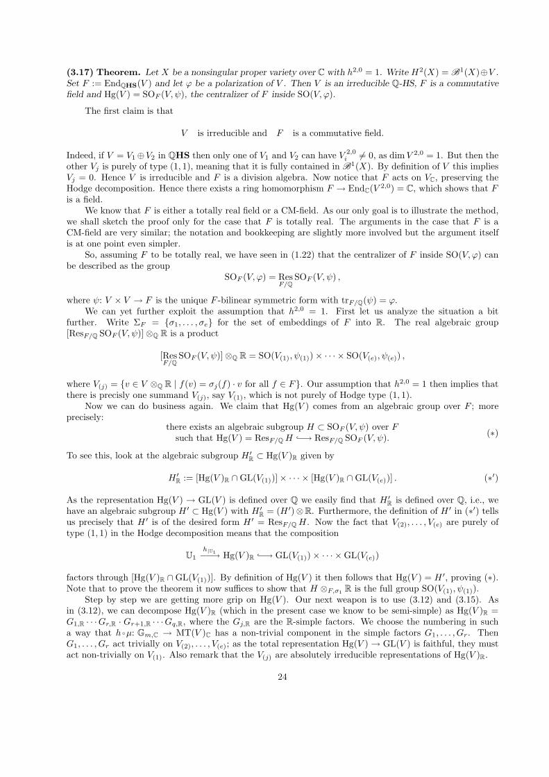
(3.17) Theorem. Let X be a nonsingular proper variety over C with h2,0 = 1. Write H2(X) = B1(X)⊕V .Set F := EndQHS(V ) and let ϕ be a polarization of V . Then V is an irreducible Q-HS, F is a commutativefield and Hg(V ) = SOF (V, ψ), the centralizer of F inside SO(V, ϕ).

The first claim is that

V is irreducible and F is a commutative field.

Indeed, if V = V1⊕V2 in QHS then only one of V1 and V2 can have V 2,0i 6= 0, as dim V 2,0 = 1. But then the

other Vj is purely of type (1, 1), meaning that it is fully contained in B1(X). By definition of V this impliesVj = 0. Hence V is irreducible and F is a division algebra. Now notice that F acts on VC, preserving theHodge decomposition. Hence there exists a ring homomorphism F → EndC(V 2,0) = C, which shows that Fis a field.

We know that F is either a totally real field or a CM-field. As our only goal is to illustrate the method,we shall sketch the proof only for the case that F is totally real. The arguments in the case that F is aCM-field are very similar; the notation and bookkeeping are slightly more involved but the argument itselfis at one point even simpler.

So, assuming F to be totally real, we have seen in (1.22) that the centralizer of F inside SO(V, ϕ) canbe described as the group

SOF (V, ϕ) = ResF/Q

SOF (V, ψ) ,

where ψ: V × V → F is the unique F -bilinear symmetric form with trF/Q(ψ) = ϕ.We can yet further exploit the assumption that h2,0 = 1. First let us analyze the situation a bit

further. Write ΣF = σ1, . . . , σe for the set of embeddings of F into R. The real algebraic group[ResF/Q SOF (V, ψ)]⊗Q R is a product

[ResF/Q

SOF (V, ψ)]⊗Q R = SO(V(1), ψ(1))× · · · × SO(V(e), ψ(e)) ,

where V(j) = v ∈ V ⊗Q R | f(v) = σj(f) · v for all f ∈ F. Our assumption that h2,0 = 1 then implies thatthere is precisly one summand V(j), say V(1), which is not purely of Hodge type (1, 1).

Now we can do business again. We claim that Hg(V ) comes from an algebraic group over F ; moreprecisely:

there exists an algebraic subgroup H ⊂ SOF (V, ψ) over Fsuch that Hg(V ) = ResF/QH −→ ResF/Q SOF (V, ψ).

(∗)

To see this, look at the algebraic subgroup H ′R ⊂ Hg(V )R given by

H ′R := [Hg(V )R ∩GL(V(1))]× · · · × [Hg(V )R ∩GL(V(e))] . (∗′)

As the representation Hg(V ) → GL(V ) is defined over Q we easily find that H ′R is defined over Q, i.e., we

have an algebraic subgroup H ′ ⊂ Hg(V ) with H ′R = (H ′)⊗R. Furthermore, the definition of H ′ in (∗′) tells

us precisely that H ′ is of the desired form H ′ = ResF/Q H . Now the fact that V(2), . . . , V(e) are purely oftype (1, 1) in the Hodge decomposition means that the composition

U1

h|U1−−→ Hg(V )R −→ GL(V(1))× · · · ×GL(V(e))

factors through [Hg(V )R ∩GL(V(1))]. By definition of Hg(V ) it then follows that Hg(V ) = H ′, proving (∗).Note that to prove the theorem it now suffices to show that H ⊗F,σ1 R is the full group SO(V(1), ψ(1)).

Step by step we are getting more grip on Hg(V ). Our next weapon is to use (3.12) and (3.15). Asin (3.12), we can decompose Hg(V )R (which in the present case we know to be semi-simple) as Hg(V )R =G1,R · · ·Gr,R · Gr+1,R · · ·Gq,R, where the Gj,R are the R-simple factors. We choose the numbering in sucha way that hµ: Gm,C → MT(V )C has a non-trivial component in the simple factors G1, . . . , Gr. ThenG1, . . . , Gr act trivially on V(2), . . . , V(e); as the total representation Hg(V )→ GL(V ) is faithful, they mustact non-trivially on V(1). Also remark that the V(j) are absolutely irreducible representations of Hg(V )R.

24

We use Lie-algebra notations as set up in (3.8) and (3.10), applied to the module W = V(1),C. Inparticular we set g = Lie(MT(V )C) and gi = Lie(Gi,C), and we write X ⊂ P0⊕P (R) for the support of W .Applying (3.12) we find that there are two possibilities:(a) r = 2 and the g1 × g2-module V(1),C is of the form ρ1 ⊠ ρ2 where ρi (i = 1, 2) is an irreducible represen-

tation of gi with highest weight λi of length 1;(b) r = 1 and V(1),C is an irreducible g1-module with highest weight λ of level ≤ 2.

Next we exploit (3.15). What we have found there means, in the present situation, that there exists anonzero Q-linear map ϕ: P0 ⊕ P (R) → Q (once again using the notations set up in (3.8) and (3.10)) withϕ(X ) contained in an arithmetic progression a0, a1, a2 of length 2, such that ϕ−1(a0) and ϕ−1(a2) consistof a single element:

•

• •

• • • ←−X := Supp(V(1))• • • •

• • •

• •

•

P0 ⊕ P (R)

yϕ

• • • Q

1 m 1

This brings us in a situation where the representation theory of semi-simple Lie algebras (much in thestyle of the first half of this section) leaves us with rather few possibilities. In fact, what possibilities are leftwas analyzed by Zarhin in [99], from which we copy the following result.

(3.18) Lemma. Let g be a semi-simple Lie algebra over an algebraically closed field of characteristic 0. LetW be a faithful irreducible g-module. Suppose there exists a nonzero homomorphism ϕ: P (R) → Q suchthat ϕ(Supp(W )) is contained in an arithmetic progression a0, a1, a2 of length 2 and such that ϕ−1(a0) andϕ−1(a2) consist of at most 1 element. Then all simple factors of g are of the same classical type Aℓ, Bℓ, Cℓ

or Dℓ, and there are only the following possibilities.(i) g ∼= slℓ+1 (type Aℓ) and W is the standard representation or its dual;(ii) W is the adjoint representation of g ∼= sl2 (note: sl2 ∼= so3);(iii) g ∼= so2ℓ+1 (type Bℓ) and W is the standard representation;(iv) g ∼= sp2ℓ (type Cℓ) and W is the standard representation;(v) g ∼= so2ℓ (type Dℓ) and W is the standard representation.

With this lemma at hand we can finish the proof of (3.17) (still assuming F to be totally real). Namely,we find that (a) is only possible if g1 × g2

∼= sl2 × sl2 with representation St⊠ St (where “St” denotesthe standard 2-dimensional representation). This can be rewritten as the standard representation of so4

∼=sl2 × sl2, case (v) of the lemma. If we are in case (b) then it follows from the lemma that g1 is isomorphicto so(V(1), ψ(1)). (Note that we are dealing with an orthogonal representation.) This shows that H ⊗F,σ1 R

is the full group SO(V(1), ψ(1)) which proves (deep breath) the claim of (3.17).

Exercise. Let V be as in (3.17). Suppose that V is of CM-type. Give a complete description of the CM-typeΦ (see (1.26)) and the Hodge group. Prove (3.17) in this case.

Note. In the second part of my course I intend to discuss how similar techniques as above can beapplied to the study of Galois representations associated to algebraic varieties over a number field. We shallfollow [62]. Basic results on Galois representations can be found in (a selection) [7], [8], [15], [23], [27], [29],

25

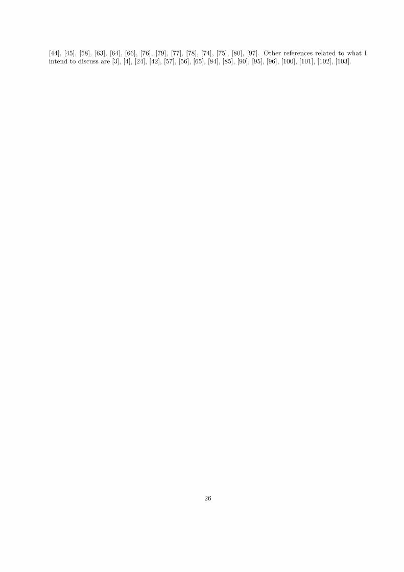
[44], [45], [58], [63], [64], [66], [76], [79], [77], [78], [74], [75], [80], [97]. Other references related to what Iintend to discuss are [3], [4], [24], [42], [57], [56], [65], [84], [85], [90], [95], [96], [100], [101], [102], [103].

26

λ =ℓ∑

i=1

mi ·i

Type of g length(λ) depth(λ)

Aℓ

ℓ∑i=1

mi

ℓ∑i=1

mi

Bℓ mℓ + 2ℓ−1∑i=1

mi mℓ + 2ℓ−1∑i=1

mi

Cℓ min(S1, S2), where m1 + 2ℓ∑

i=2

mi

S1 := 2ℓ∑

i=1

mi , S2 :=ℓ∑

i=1

imi

Dℓ min(S1, S2), if ℓ is odd, m1 +mℓ−1 +mℓ + 2ℓ−2∑i=2

mi

min(S1, S3, S4), if ℓ is even, where

S1 := mℓ−1 +mℓ + 2ℓ−2∑i=1

mi

S2 := (ℓ−1)(mℓ−1+mℓ)2 +

ℓ−2∑i=1

imi

S3 := ℓmℓ−1+(ℓ−2)mℓ

2 +ℓ−2∑i=1

imi

S4 := (ℓ−2)mℓ−1+ℓmℓ

2 +ℓ−2∑i=1

imi

E6 2m1 + 2m2 + 3m3 + 4m4 m1 + 2m2 + 2m3 + 3m4

+3m5 + 2m6 +2m5 +m6

E7 min(S1, S2), where 2m1 + 2m2 + 3m3 + 4m4

S1 := 2m1 + 3m2 + 4m3 +3m5 + 2m6 +m7

+6m4 + 5m5 + 4m6 + 3m7,

S2 := 4m1 + 4m2 + 6m3

+8m4 + 6m5 + 4m6 + 2m7

E8 4m1 + 6m2 + 8m3 + 12m4 2m1 + 3m2 + 4m3 + 6m4

+10m5 + 8m6 + 6m7 + 4m8 +5m5 + 4m6 + 3m7 + 2m8

F4 4m1 + 6m2 + 4m3 + 2m4 2m1 + 4m2 + 3m3 + 2m4

G2 2m1 + 4m2 2m1 + 3m2

Table 1. Length and depth of the dominant weights in the simple root sytems.

27

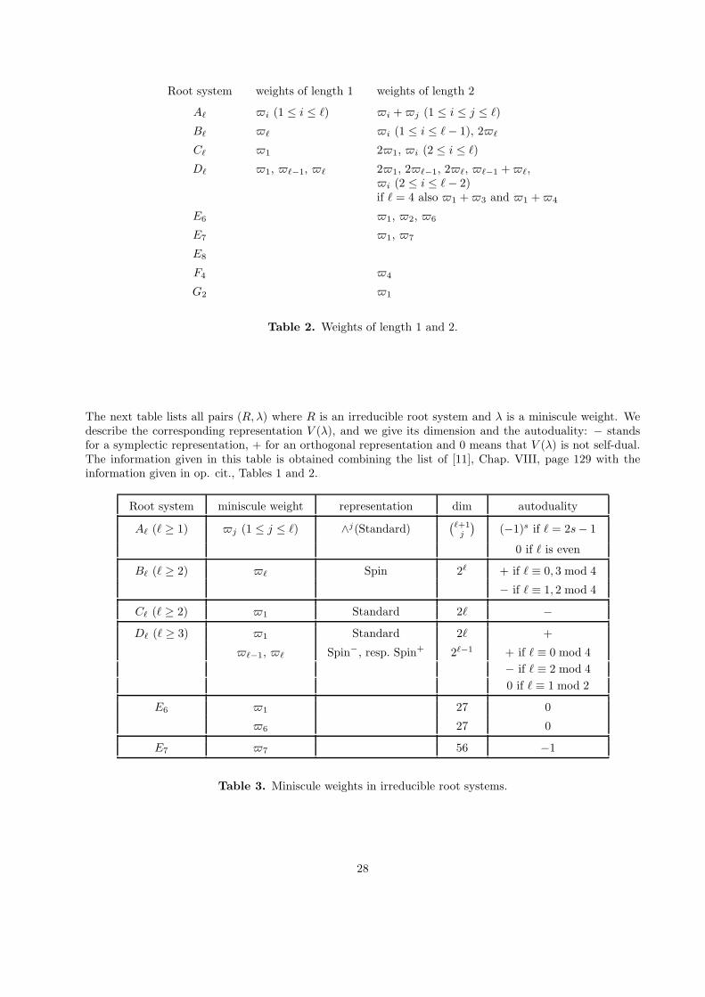
Root system weights of length 1 weights of length 2

Aℓ i (1 ≤ i ≤ ℓ) i +j (1 ≤ i ≤ j ≤ ℓ)

Bℓ ℓ i (1 ≤ i ≤ ℓ− 1), 2ℓ

Cℓ 1 21, i (2 ≤ i ≤ ℓ)

Dℓ 1, ℓ−1, ℓ 21, 2ℓ−1, 2ℓ, ℓ−1 +ℓ,i (2 ≤ i ≤ ℓ− 2)if ℓ = 4 also 1 +3 and 1 +4

E6 1, 2, 6

E7 1, 7

E8

F4 4

G2 1

Table 2. Weights of length 1 and 2.

The next table lists all pairs (R, λ) where R is an irreducible root system and λ is a miniscule weight. Wedescribe the corresponding representation V (λ), and we give its dimension and the autoduality: − standsfor a symplectic representation, + for an orthogonal representation and 0 means that V (λ) is not self-dual.The information given in this table is obtained combining the list of [11], Chap. VIII, page 129 with theinformation given in op. cit., Tables 1 and 2.

Root system miniscule weight representation dim autoduality

Aℓ (ℓ ≥ 1) j (1 ≤ j ≤ ℓ) ∧j(Standard)(ℓ+1

j

)(−1)s if ℓ = 2s− 1

0 if ℓ is even

Bℓ (ℓ ≥ 2) ℓ Spin 2ℓ + if ℓ ≡ 0, 3 mod 4

− if ℓ ≡ 1, 2 mod 4

Cℓ (ℓ ≥ 2) 1 Standard 2ℓ −

Dℓ (ℓ ≥ 3) 1 Standard 2ℓ +

ℓ−1, ℓ Spin−, resp. Spin+ 2ℓ−1 + if ℓ ≡ 0 mod 4

− if ℓ ≡ 2 mod 4

0 if ℓ ≡ 1 mod 2

E6 1 27 0

6 27 0

E7 7 56 −1

Table 3. Miniscule weights in irreducible root systems.

28

References

[1] Abdulali, S. Abelian varieties and the general Hodge conjecture. Compositio Math. 109 (1997), 341–355.

[2] Andre, Y. Mumford-Tate groups of mixed Hodge structures and the theorem of the fixed part. CompositioMath. 82 (1992), 1–24.

[3] Andre, Y. On the Shafarevich and Tate conjectures for hyper-Kahler varieties. Math. Ann. 305 (1996),205–248.

[4] Andre, Y. Pour une theorie inconditionnelle des motifs. Publ. Math. IHES 83 (1996), 5–49.

[5] Atiyah, M., and Hirzebruch, F. Analytic cycles on complex manifolds. Topology 1 (1962), 25–45.

[6] Barton, C., and Clemens, C. A result on the integral chow ring of a generic principally polarized complexabelian variety of dimension four. Compos. Math. 34 (1977), 49–67.

[7] Blasius, D. A p-adic property of Hodge classes on abelian varieties. In Jannsen et al. [40], pp. 293–308(Part 2).

[8] Bogomolov, F. A. Sur l’algebricite des representations l-adiques. C. R. Acad. Sci. Paris Ser. A-B 290(1980), A701–A703.

[9] Borel, A. Linear algebraic groups, second ed. Graduate Texts in Math. 126. Springer-Verlag, New York,1991.

[10] Bourbaki, N. Elements de mathematique. Groupes et algebres de Lie. Chapitres IV–VI. Masson, Paris,1981.

[11] Bourbaki, N. Elements de mathematique. Groupes et algebres de Lie. Chapitres VII et VIII (Nouveautirage). Masson, Paris, 1990.

[12] Brylinski, J.-L. “1-motifs” et formes automorphes (theorie arithmetique des domaines de Siegel). InJournees automorphes (Dijon, 1981), Publ. Math. de l’Universite Paris VII, Vol. 15. Univ. Paris VII,Paris, 1983, pp. 43–106.

[13] Brylinski, J.-L., and Zucker, S. An overview of recent advances in Hodge theory. In Several complex variables,VI. Springer-Verlag, Berlin, 1990, pp. 39–142.

[14] Carlson, J., Green, M., Griffiths, P., and Harris, J. Infinitesimal variations of Hodge structure. I. CompositioMath. 50 (1983), 109–205.

[15] Chi, W. C. l-adic and λ-adic representations associated to abelian varieties defined over number fields.Amer. J. Math. 114 (1992), 315–353.

[16] Deligne, P. Theorie de Hodge. II. Publ. Math. IHES 40 (1971), 5–57.

[17] Deligne, P. Travaux de Griffiths. In Seminaire Bourbaki (1969/70), Exp. No. 376, Lecture Notes in Math.180. Springer-Verlag, Berlin, 1971, pp. 213–237.

[18] Deligne, P. Travaux de Shimura. In Seminaire Bourbaki (1970/71), Exp. No. 389, Lecture Notes in Math.244. Springer-Verlag, Berlin, 1971, pp. 123–165.

[19] Deligne, P. La conjecture de Weil pour les surfaces K3. Invent. Math. 15 (1972), 206–226.

[20] Deligne, P. Theorie de Hodge. III. Publ. Math. IHES 44 (1974), 5–77.

[21] Deligne, P. Varietes de Shimura: interpretation modulaire, et techniques de construction de modelescanoniques. In Automorphic forms, representations, and L-functions, A. Borel and W. Casselman,Eds., Proc. Sympos. Pure Math. 33. Amer. Math. Soc., Providence, R.I., 1979, pp. 247–289.

[22] Deligne, P. Cycles de Hodge absolus et periodes des integrales des varietes abeliennes. Mem. Soc. Math.France (N.S.) 2 (1980/81), 23–33.

29

[23] Deligne, P. Hodge cycles on abelian varieties (notes by J. S. Milne). In Hodge cycles, motives andShimura varieties [26], pp. 9–100.

[24] Deligne, P. A quoi servent les motifs? In Jannsen et al. [40], pp. 143–161 (Part 1).

[25] Deligne, P., and Milne, J. S. Tannakian categories. In Hodge cycles, motives, and Shimura varieties [26],pp. 101–228.

[26] Deligne, P., Milne, J. S., Ogus, A., and Shih, K.-y. Hodge cycles, motives, and Shimura varieties. Lecture Notesin Math. 900. Springer-Verlag, Berlin, 1982.

[27] Fontaine, J.-M. Le corps des periodes p-adiques (avec un appendice par Pierre Colmez). In Periodesp-adiques [28], pp. 59–111. Seminaire de Bures, 1988, Asterisque 223 (1994).

[28] Fontaine, J.-M., Ed. Periodes p-adiques (Montrouge, 1994), Societe Mathematique de France. Seminairede Bures, 1988, Asterisque 223 (1994).

[29] Fontaine, J.-M. Representations p-adiques semi-stables. In Periodes p-adiques [28], pp. 113–184. Seminairede Bures, 1988, Asterisque 223 (1994).

[30] Gordon, B. B. A survey of the Hodge conjecture for abelian varieties. Available as alg-geom/9709030;to be published as an appendix in the second edition of [46], 1997.

[31] Griffiths, P., Ed. Topics in transcendental algebraic geometry (Princeton, NJ, 1984), Princeton UniversityPress.

[32] Griffiths, P., and Harris, J. Infinitesimal variations of Hodge structure. II. An infinitesimal invariant ofHodge classes. Compositio Math. 50 (1983), 207–265.

[33] Griffiths, P. A. Infinitesimal variations of Hodge structure. III. Determinantal varieties and the infinites-imal invariant of normal functions. Compositio Math. 50 (1983), 267–324.

[34] Gross, B., and Savin, G. Motives with Galois group of type G2: an exceptional theta correspondence.Compositio Math. 114 (1998), 153–217.

[35] Gross, B. H. A remark on tube domains. Math. Res. Lett. 1 (1994), 1–9.

[36] Grothendieck, A. Hodge’s general conjecture is false for trivial reasons. Topology 8 (1969), 299–303.

[37] Hazama, F. Algebraic cycles on certain abelian varieties and powers of special surfaces. J. Fac. Sci. Univ.Tokyo Sect. IA Math. 31 (1985), 487–520.

[38] Hazama, F. Algebraic cycles on nonsimple abelian varieties. Duke Math. J. 58 (1989), 31–37.

[39] Hazama, F. The generalized Hodge conjecture for stably nondegenerate abelian varieties. CompositioMath. 93 (1994), 129–137.

[40] Jannsen, U., Kleiman, S., and Serre, J.-P., Eds. Motives (Providence, RI, 1994), Proc. Symposia Pure Math.55, American Mathematical Society.

[41] Knus, M.-A., Merkurjev, A., Rost, M., and Tignol, J.-P. The book of involutions. American Mathematical Society,Providence, RI, 1998.

[42] Kottwitz, R. E. Isocrystals with additional structure. Compositio Math. 56 (1985), 201–220.

[43] Kottwitz, R. E. Points on some Shimura varieties over finite fields. J. Amer. Math. Soc. 5 (1992), 373–444.

[44] Larsen, M., and Pink, R. On l-independence of algebraic monodromy groups in compatible systems ofrepresentations. Invent. Math. 107 (1992), 603–636.

[45] Larsen, M., and Pink, R. Abelian varieties, l-adic representations, and l-independence. Math. Ann. 302(1995), 561–579.

[46] Lewis, J. D. A survey of the Hodge conjecture. Universite de Montreal Centre de RecherchesMathematiques, Montreal, PQ, 1991.

30

[47] Looijenga, E., and Lunts, V. A. A Lie algebra attached to a projective variety. Invent. Math. 129 (1997),361–412.

[48] Milne, J. S. Shimura varieties and motives. In Jannsen et al. [40], pp. 447–523 (Part 2).

[49] Moonen, B. J. J., and Zarhin, Y. G. Hodge classes on abelian varieties of low dimension. Utrecht Univ.preprint 1087, Jan. 1999. Also available as math.AG/9901113.

[50] Moonen, B. J. J., and Zarhin, Y. G. Hodge classes and Tate classes on simple abelian fourfolds. Duke Math.J. 77 (1995), 553–581.

[51] Moonen, B. J. J., and Zarhin, Y. G. Weil classes on abelian varieties. J. Reine Angew. Math. 496 (1998),83–92.

[52] Mumford, D. A note of Shimura’s paper “Discontinuous groups and abelian varieties”. Math. Ann. 181(1969), 345–351.

[53] Mumford, D. Abelian varieties. Oxford Univ. Press, Oxford, 1970. Tata Institute of FundamentalResearch Studies in Mathematics, No. 5.

[54] Murty, V. K. Exceptional Hodge classes on certain abelian varieties. Math. Ann. 268 (1984), 197–206.

[55] Murty, V. K. The Hodge group of an abelian variety. Proc. Amer. Math. Soc. 104 (1988), 61–68.

[56] Noot, R. Abelian varieties arising from Mumford’s Shimura curves. Institut de recherche mathematiquede Rennes, Univ. de Rennes 1, prepublication 97-26, 1997.

[57] Noot, R. Abelian varieties—Galois representations and properties of ordinary reduction. CompositioMath. 97 (1995), 161–171.

[58] Ogus, A. A p-adic analogue of the Chowla-Selberg formula. In p-adic analysis (Trento, 1989), F. Bal-dassari et al., Eds., Lecture Notes in Math. 1454. Springer-Verlag, Berlin, 1990, pp. 319–341.

[59] Oort, F. Endomorphism algebras of abelian varieties. In Algebraic geometry and commutative algebrain honor of Masayoshi Nagata, Vol. II (Tokyo, 1988), H. Hijikata et al., Eds., Kinokuniya Company,Ltd., pp. 469–502.

[60] Peters, C., and Steenbrink, J. Infinitesimal variations of Hodge structure and the generic Torelli problem forprojective hypersurfaces (after Carlson, Donagi, Green, Griffiths, Harris). In Classification of algebraicand analytic manifolds (Katata, 1982). Birkhauser Boston, Boston, Mass., 1983, pp. 399–463.

[61] Pink, R. Arithmetical compactification of mixed Shimura varieties. Universitat Bonn MathematischesInstitut, Bonn, 1990. Dissertation, Rheinische Friedrich-Wilhelms-Universitat Bonn, Bonn, 1989.

[62] Pink, R. l-adic algebraic monodromy groups, cocharacters, and the Mumford-Tate conjecture. J. ReineAngew. Math. 495 (1998), 187–237.

[63] Pjateckiı-Sapiro, I. I. Interrelations between the Tate and Hodge hypotheses for abelian varieties. Mat.Sb. (N.S.) 85 (1971), 610–620.

[64] Pohlmann, H. Algebraic cycles on abelian varieties of complex multiplication type. Ann. of Math. 88(1968), 161–180.

[65] Rapoport, M., and Richartz, M. On the classification and specialization of F -isocrystals with additionalstructure. Compositio Math. 103 (1996), 153–181.

[66] Ribet, K. A. Galois action on division points of Abelian varieties with real multiplications. Amer. J.Math. 98 (1976), 751–804.

[67] Ribet, K. A. Hodge classes on certain types of abelian varieties. Amer. J. Math. 105 (1983), 523–538.

[68] Saavedra Rivano, N. Categories Tannakiennes. Lecture Notes in Math. 265. Springer-Verlag, Berlin, 1972.Lecture Notes in Mathematics, Vol. 265.

31

[69] Satake, I. Algebraic structures of symmetric domains. Iwanami Shoten, Tokyo, 1980.

[70] Schappacher, N. Periods of Hecke characters. Lecture Notes in Math. 1301. Springer-Verlag, Berlin, 1988.

[71] Schoen, C. Hodge classes on self-products of a variety with an automorphism. Compositio Math. 65(1988), 3–32.

[72] Schoen, C. Cyclic covers of Pv branched along v + 2 hyperplanes and the generalized Hodge conjecturefor certain abelian varieties. In Arithmetic of complex manifolds (Erlangen, 1988), Lecture Notes inMath. 1399. Springer-Verlag, Berlin, 1989, pp. 137–154.

[73] Schoen, C. Addendum to: “Hodge classes on self-products of a variety with an automorphism”. Compo-sitio Math. 114 (1998), 329–336.

[74] Serre, J.-P. Letters to Ken Ribet, 1 January and 29 January, 1981.

[75] Serre, J.-P. Letter to John Tate, 2 January, 1985.

[76] Serre, J.-P. Sur les groupes de Galois attaches aux groupes p-divisibles. In Proc. Conf. Local Fields(Driebergen, 1966). Springer-Verlag, Berlin, 1967, pp. 118–131.

[77] Serre, J.-P. Representations l-adiques. Japan Soc. Promotion Sci., Tokyo, 1977, pp. 177–193.

[78] Serre, J.-P. Groupes algebriques associes aux modules de Hodge-Tate. In Journees de GeometrieAlgebrique de Rennes. (Rennes, 1978), Vol. III. Soc. Math. France, Paris, 1979, pp. 155–188.

[79] Serre, J.-P. Abelian l-adic representations and elliptic curves (Reissue). Advanced book classics. Addison-Wesley, Redwood City, 1989.

[80] Serre, J.-P. Proprietes conjecturales des groupes de Galois motiviques et des representations l-adiques.In Jannsen et al. [40], pp. 377–400 (Part 1).

[81] Shimura, G. On analytic families of polarized abelian varieties and automorphic functions. Ann. of Math.78 (1963), 149–192.

[82] Shioda, T. Algebraic cycles on abelian varieties of Fermat type. Math. Ann. 258 (1981/82), 65–80.

[83] Shioda, T. What is known about the Hodge conjecture? In Algebraic varieties and analytic varieties(Tokyo, 1981). North-Holland, Amsterdam, 1983, pp. 55–68.

[84] Silverberg, A., and Zarhin, Y. G. Connectedness results for l-adic representations associated to abelianvarieties. Compositio Math. 97 (1995), 273–284.

[85] Silverberg, A., and Zarhin, Y. G. Connectedness extensions for abelian varieties. Math. Z. 228, 2 (1998),387–403.

[86] Steenbrink, J., and Zucker, S. Variation of mixed Hodge structure. I. Invent. Math. 80 (1985), 489–542.

[87] Steenbrink, J. H. M. Some remarks about the Hodge conjecture. In Hodge theory (Sant Cugat, 1985),Lecture Notes in Math. 1246. Springer-Verlag, Berlin, 1987, pp. 165–175.

[88] Tankeev, S. G. On algebraic cycles on abelian varieties. II. Math. USSR-Izv. 14 (1980), 383–394.

[89] Tankeev, S. G. Cycles on simple abelian varieties of prime dimension. Math. USSR-Izv. 20 (1983),157–171.

[90] Tankeev, S. G. Surfaces ofK3 type over number fields and the Mumford-Tate conjecture. Math USSR-Izv.37 (1991), 191–208.

[91] Tankeev, S. G. Abelian varieties and the general Hodge conjecture. Russian Acad. Sci. Izv. Math. 43(1994), 179–191.

[92] van Geemen, B. An introduction to the Hodge conjecture for abelian varieties. In Algebraic cycles andHodge theory (Torino, 1993), Lecture Notes in Math. 1594. Springer-Verlag, Berlin, 1994, pp. 233–252.

32

[93] van Geemen, B. Theta functions and cycles on some abelian fourfolds. Math. Z. 221 (1996), 617–631.

[94] Weil, A. Abelian varieties and the Hodge ring. In Collected papers. Vol. III, [1977c]. Springer-Verlag,New York, 1979, pp. 421–429.

[95] Wintenberger, J.-P. Un scindage de la filtration de Hodge pour certaines varietes algebriques sur les corpslocaux. Ann. of Math. 119 (1984), 511–548.

[96] Wintenberger, J.-P. Relevement selon une isogenie de systemes l-adiques de representations galoisiennesassocies aux motifs. Invent. Math. 120 (1995), 215–240.

[97] Zarhin, Y. G. Abelian varieties, l-adic representations and Lie algebras. Rank independence on l. Invent.Math. 55 (1979), 165–176.

[98] Zarhin, Y. G. Hodge groups of K3 surfaces. J. Reine Angew. Math. 341 (1983), 193–220.

[99] Zarhin, Y. G. Weights of simple Lie algebras in the cohomology of algebraic varieties. Math. USSR-Izv.24 (1985), 245–281.

[100] Zarhin, Y. G. Abelian varieties of K3 type and l-adic representations. In Algebraic geometry and analyticgeometry (Tokyo, 1990), A. Fujiki et al., Eds. Springer-Verlag, Tokyo, 1991, pp. 231–255.

[101] Zarhin, Y. G. Abelian varieties having a reduction of K3 type. Duke Math. J. 65 (1992), 511–527.

[102] Zarhin, Y. G. Abelian varieties of K3 type. In Seminaire de Theorie des Nombres, Paris, 1990–91.Birkhauser Boston, Boston, MA, 1993, pp. 263–279.

[103] Zarhin, Y. G. CM abelian varieties with almost ordinary reduction. In Number theory (Paris, 1992–1993).Cambridge Univ. Press, Cambridge, 1995, pp. 277–291.

Ben Moonen, University of Utrecht, Department of Mathematics, P.O. Box 80.010, NL-3508 TA Utrecht,The Netherlands. E-mail: moonen@math.uu.nl

33