Notes on Modern Cosmology - sackett.netsackett.net/BillDLiddleNotes.pdf · Notes on An Introduction...

Notes on An Introduction to Modern Cosmologyby Andrew Liddle(with additional material from other sources)Prepared by Bill Daniel

1 Preliminary Concepts

ü 1.1 Large-Scale Characteristics of the Universe

The cosmological principle is the unproven but well-supported assumption that, ignoring local variations (which can be huge),any place in the universe is no more special than any other place. This is equivalent to saying that the universe is spatially bothhomogeneous (looks the same at each point) and isotropic (looks the same in every direction). Homogeneity does not implyisotropy, but universal isotropy does imply homogeneity. The cosmological principle is obviously not true at the scale of thesolar system, the galaxy, or even galaxy clusters, but, making this assumption for the universe as a whole has profound andpowerful cosmological consequences.

It would seem that the expansion of the universe violates the cosmological principle, since we appear to be in a privilegedlocation at the center of the expansion, with expansion rates proportional to distance away from us. This does not violate thecosmological principle, though, since an observer at any point in the universe would see the expansion as centered on them withthe same proportionality between recession rate and distance that we see.

The perfect cosmological principle, the idea that the universe is both spatially homogeneous and isotropic as well as homoge-neous in time, was the basis of the steady-state theory and appears to be almost certainly wrong.

ü 1.2 Redshift, z, and Hubbleʼs Law

The redshift of spectral lines is defined observationally as z = lobs-lemlem

. Redshift is related to the magnitude of the recessionary

(radial) velocity of a galaxy, u, as u = z c. A galaxy’s recessionary velocity is composed of two parts; a radial velocity due toexpansion of the universe and a randomly oriented peculiar velocity due to gravitational perturbations induced by other nearbymatter. The peculiar velocity makes Hubble’s Law, v = H0 r, approximate, with the approximation being worse for nearbygalaxies.

The proportionality constant, H0, is called the Hubble parameter (or Hubble constant, though it’s not actually constantHH = HHtL) over cosmological time). The zero subscript in this symbol, and other symbols in his document, refers to the value ofthat quantity at the present time. Note that the assumption of isotropy requires that H ¹≠ HHq, fL, and so expansion is purelyradial. Measurements of H0 are notoriously difficult and their uncertainty is parameterized by h (not to be confused with Plank’sconstant), as:

H0 = 100 h kg ÿsec-1 ÿMpc-1 = h9.8µ109 yr

= 2.13 h µ 10-33 eV ÿ h-1 with h = 0.72 ± 0.02.

The above expression for H0, while useful when thinking of it as a measure of the recessionary velocity of the expandinguniverse, obscures another, equally important way of thinking about the Hubble parameter. Changing the units gives,H0

-1 = 9.77 h-1µ109yrs, called the Hubble time, a crude estimate of the age of the universe - crude because it ignores changes inthe expansionary velocity over the history of the universe.

The redshift of spectral lines is defined observationally as z = lobs-lemlem

. Redshift is related to the magnitude of the recessionary

(radial) velocity of a galaxy, u, as u = z c. A galaxy’s recessionary velocity is composed of two parts; a radial velocity due toexpansion of the universe and a randomly oriented peculiar velocity due to gravitational perturbations induced by other nearbymatter. The peculiar velocity makes Hubble’s Law, v = H0 r, approximate, with the approximation being worse for nearbygalaxies.

The proportionality constant, H0, is called the Hubble parameter (or Hubble constant, though it’s not actually constantHH = HHtL) over cosmological time). The zero subscript in this symbol, and other symbols in his document, refers to the value ofthat quantity at the present time. Note that the assumption of isotropy requires that H ¹≠ HHq, fL, and so expansion is purelyradial. Measurements of H0 are notoriously difficult and their uncertainty is parameterized by h (not to be confused with Plank’sconstant), as:

H0 = 100 h kg ÿsec-1 ÿMpc-1 = h9.8µ109 yr

= 2.13 h µ 10-33 eV ÿ h-1 with h = 0.72 ± 0.02.

The above expression for H0, while useful when thinking of it as a measure of the recessionary velocity of the expandinguniverse, obscures another, equally important way of thinking about the Hubble parameter. Changing the units gives,H0

-1 = 9.77 h-1µ109yrs, called the Hubble time, a crude estimate of the age of the universe - crude because it ignores changes inthe expansionary velocity over the history of the universe.

ü 1.3 The Scale Factor, a(t)

The time-dependent Hubble “constant” is defined in terms of the scale factor, aHtL, as HHtL ª aÿ HtLaHtL

. The scale factor measures how

physical dimensions change with time. The redshift is a natural consequence of the Doppler effect which stretches wavelengthsas, lobs = lem aHtobsL êaHtemL. Combining this with the above and relabeling aHtobsL = a0 = 1 gives,

z = 1-aHtemLaHtemL

or aHzL = 11+z

.

ü 1.4 Comoving Coordinates

Because general relativity (GR) requires that the laws of physics are the same in any coordinate system, including non-inertialones, we can choose to work in any convenient coordinate system. We will often choose to use comoving coordinates, x, thatare carried along with the universal expansion, rather than physical coordinates, r, which define a fixed coordinate system inwhich the expansion takes place. These physical coordinates are those we live in on earth (and anywhere within the galaxy) andthose of any bound system, that are not affected by the expansion of the universe.

The transformation between these coordinate systems is given by, r = aHtL x. Note that, for objects that are stationary relative to

the observer, x×= 0, but r

×= a

ÿHtL x. Note also that our assumption of isotropy is only true for comoving coordinate systems.

The comoving horizon is defined as the surface of a sphere centered on the observer whose radius is the distance light could havetraveled in the absence of interactions since the origin of the universe. It defines the observable universe. Due to the expansionof the universe, its radius is not simply the age of the universe times the speed of light.

To locate the comoving horizon, we need another concept called the conformal time, h. In time interval d t, light in an expand-

ing universe with scale factor aHtL will have traveled a distance d h = d xa= c d t

a. Setting c = 1, we write, h ª Ÿ0

t d t£

aHt£L. The confor-

mal time is not any physically meaningful time, but h0 is the time it would take a photon to travel from our current location to theedge of the observable universe, if the universe were to suddenly stop expanding. The comoving horizon is at a distance equal toc times the conformal time.

ü 1.5 Curvature, k

The cosmological principle demands that space must exhibit the same overall curvature at every point. Local variations incurvature, just like local variations in mass-energy density, r, are of course, tolerated. There are only three spatial geometriesthat allow constant curvature: flat space, uniformly positively curved (closed) space, or uniformly negatively curved (open)space. We will address curvature in more detail in the section on GR, but for our purposes now, we can capture what we need ofcurvature in a single number, the curvature parameter, k. Curvature is determined by the mass-energy density of the universe.There is a particular value of mass-energy density, called the critical density, rc, that must exist for the curvature of spacetime tobe flat. Universes with r < rc are open, while those with r > rc are closed.

We can force k to take on one of three discrete values: zero for flat space, +1 for closed space and -1 for open space. Althoughwe can’t draw 3-dimensional curved spaces, we can get a feel for their behavior by considering curved 2-dimensional surfaces.

For the “flat” (or Euclidean) space we are used to, geometric figures behave the way we were taught in school. The shortestdistance between two points is a straight line. Flat universes are infinite, since, if they had an edge, the cosmological principlewould fail there. No points in flat space are any more “special” than any other point.

A non-rotating 2-dimensional spherical surface also has no “special” locations. If its radius is finite, it has no edge, but has afinite area, 4 p r2. Geometric figures on a sphere behave strangely, with the angles of a triangle adding up to more than 180È andthe circumference of a circle being less than 2 p r. “Straight lines” don’t exist on a spherical surface and the shortest distancebetween points is the arc of a great circle - a circle that defines a plane that passes through the center of the sphere. Great circlesin a spherical geometry are examples of the more general concept of a geodesic - the curve that defines the “shortest distance”between two points in any space, regardless of its curvature.

Negative curvature is usually modeled in 2-dimensional space by a saddle-shaped surface. This not a perfect analog for the 3-dimensional version, since it’s not possible to construct a 2-dimensional surface of uniformly constant negative curvature in 3-dimensional space. The saddle-shaped surface will only have constant curvature at the center point of the saddle. Thus, thecenter point is unique, meaning that it also violates the cosmological principle. Nevertheless, the approximation shows that theangles of a triangle in negatively curved space add up to less than 180È and the circumference of a circle is more than 2 p r.

2 Notes on Modern Cosmology.nb

The cosmological principle demands that space must exhibit the same overall curvature at every point. Local variations incurvature, just like local variations in mass-energy density, r, are of course, tolerated. There are only three spatial geometriesthat allow constant curvature: flat space, uniformly positively curved (closed) space, or uniformly negatively curved (open)space. We will address curvature in more detail in the section on GR, but for our purposes now, we can capture what we need ofcurvature in a single number, the curvature parameter, k. Curvature is determined by the mass-energy density of the universe.There is a particular value of mass-energy density, called the critical density, rc, that must exist for the curvature of spacetime tobe flat. Universes with r < rc are open, while those with r > rc are closed.

We can force k to take on one of three discrete values: zero for flat space, +1 for closed space and -1 for open space. Althoughwe can’t draw 3-dimensional curved spaces, we can get a feel for their behavior by considering curved 2-dimensional surfaces.

For the “flat” (or Euclidean) space we are used to, geometric figures behave the way we were taught in school. The shortestdistance between two points is a straight line. Flat universes are infinite, since, if they had an edge, the cosmological principlewould fail there. No points in flat space are any more “special” than any other point.

A non-rotating 2-dimensional spherical surface also has no “special” locations. If its radius is finite, it has no edge, but has afinite area, 4 p r2. Geometric figures on a sphere behave strangely, with the angles of a triangle adding up to more than 180È andthe circumference of a circle being less than 2 p r. “Straight lines” don’t exist on a spherical surface and the shortest distancebetween points is the arc of a great circle - a circle that defines a plane that passes through the center of the sphere. Great circlesin a spherical geometry are examples of the more general concept of a geodesic - the curve that defines the “shortest distance”between two points in any space, regardless of its curvature.

Negative curvature is usually modeled in 2-dimensional space by a saddle-shaped surface. This not a perfect analog for the 3-dimensional version, since it’s not possible to construct a 2-dimensional surface of uniformly constant negative curvature in 3-dimensional space. The saddle-shaped surface will only have constant curvature at the center point of the saddle. Thus, thecenter point is unique, meaning that it also violates the cosmological principle. Nevertheless, the approximation shows that theangles of a triangle in negatively curved space add up to less than 180È and the circumference of a circle is more than 2 p r.

ü 1.6 The Energy-momentum Relation

The energy of any particle is given by Einstein’s famous E = m c2 when we understand E to be the particle’s total energy and mto be its relativistic mass, composed of its rest mass, m0, and the additional mass that results from its velocity. A more usefulversion of this equation, known as the energy-momentum relation, expresses how these two components combine to form theparticle’s total energy by expressing E as a function of the rest mass and the magnitude of the particle’s momentum, p,

E2 = m02 c4 + p2 c2.

Important special cases of this relation are:1) Massless particles (m0 = 0) such as photons: These relativistic particles have an energy associated only with their

motion, E = c p. This expression for radiation energy was extended in the quantum theory as (taking c = 1), E = h f = hl= —w.

Combining these equations gives the de Broglie relation, l = hp

.

2) Massive relativistic particles: These are particles, such as cosmic rays, that are moving relative to us at speeds, u,approaching c. They can never move at exactly the speed of light, since then their momentum, p = g m0 u, and hence theirenergy, would become infinite (g = 1

1-HuêcL2). Both terms in their energy-momentum relation are significant contributors to

their total energy. 3) Non-relativistic particles Hu ` c): The first two terms of the Taylor expansion of the energy-momentum relation for

small u gives E @ m0 c2 + p2

2m0; simply the sum of the particle’s rest mass energy and its classical kinetic energy (recall that

classically p = m0 u, so K.E. = p2

2m0= 12

m0 u2).

ü 1.7 The Fundamental Constituents of the Universe

There are several broad categories of constituents of our universe.

ü 1.7.1 Baryons

Baryons are usually thought of as particles composed of 3 quarks, but cosmologists also lump mesons (composed of 2 quarks)and electrons (a type of lepton - not quark-based at all) under this heading. The justification for this seems to be that, of theseparticles, only protons and neutrons (both baryons in the traditional sense) contribute in any significant way to the mass of theuniverse. Since charge neutrality arguments mean that there must be the same number of electrons as protons, and protons arealmost 2000 times more massive, the mass of the electrons in the universe is swamped by that of the protons. All other baryonsare unstable and decay into protons and neutrons, so they also can be ignored. Thus, when cosmologists say “baryons,” what ismeant is nucleons - protons and neutrons.

In the present universe, baryons are typically moving much less than light speed, so they fall into the non-relativistic category (3)above.

Notes on Modern Cosmology.nb 3

Baryons are usually thought of as particles composed of 3 quarks, but cosmologists also lump mesons (composed of 2 quarks)and electrons (a type of lepton - not quark-based at all) under this heading. The justification for this seems to be that, of theseparticles, only protons and neutrons (both baryons in the traditional sense) contribute in any significant way to the mass of theuniverse. Since charge neutrality arguments mean that there must be the same number of electrons as protons, and protons arealmost 2000 times more massive, the mass of the electrons in the universe is swamped by that of the protons. All other baryonsare unstable and decay into protons and neutrons, so they also can be ignored. Thus, when cosmologists say “baryons,” what ismeant is nucleons - protons and neutrons.

In the present universe, baryons are typically moving much less than light speed, so they fall into the non-relativistic category (3)above.

ü 1.7.2 Radiation

By “radiation”cosmologists mean electromagnetic radiation - photons - and do not include a, b, or neutron radiation. Theionizing properties of energetic photons are especially important cosmologically, so it may be useful to review the physics ofelectromagnetic radiation.

In systems that are at equilibrium, some quantity is exchanged between the elements of the system in such a way that allmicrostates (configurations of its constituents) available to the system are equally probable. The science of thermodynamicsstudies several types of equilibria - each with its own exchanged quantity. These are shown below.

Equilibrium type Exchanged quantitythermal energy

mechanical volumediffusive matter

All of these equilibria are important in cosmology, but we will focus here on thermal equilibrium among photons. Because theyare quantum mechanical particles, photons obey quantum statistics - the study of dense systems in which two or more identicalparticles have a reasonable chance of trying to occupy the same single particle state. Since photons are bosons (integer spin;spin-1 for photons), an unlimited number of them can occupy the same state.

In most gases with which we are familiar, the inter-particle distance is large compared with the particle’s de Broglie wavelength(so that the wave functions of the particles in the gas do not overlap), but in the very dense conditions of the early universe, thissimplifying assumption breaks down. It can be shown that, under these conditions in which quantum effects become important,the occupancy number of the ith state (average number of bosons in the state) is,

niBE = giíJexpJ ei-mkB T

N - 1N, where gi is the degeneracy of the state, ei is its energy, m is the chemical potential,

kB = 8.6µ10-5 eV ÿK-1 is Boltzmann’s constant and T is the temperature in Kelvins.

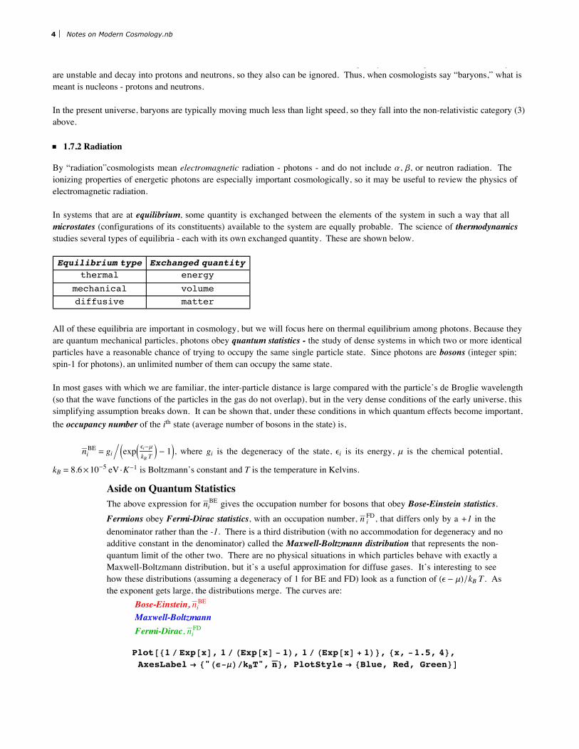
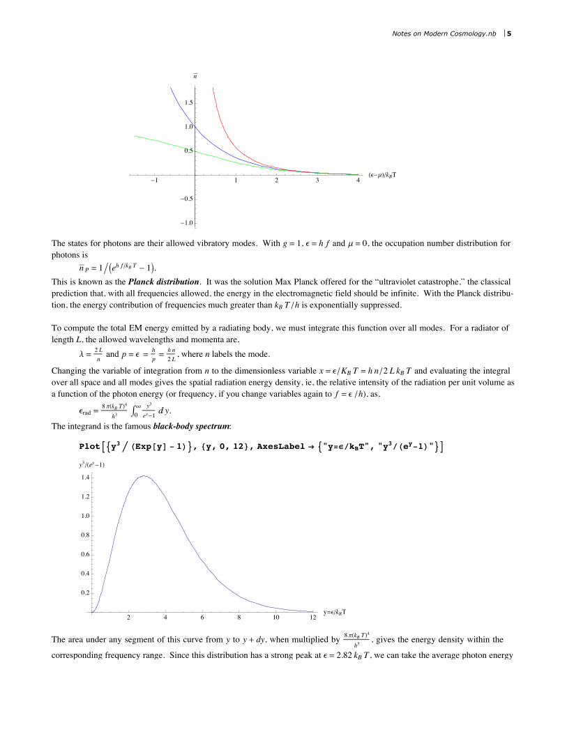
Aside on Quantum StatisticsThe above expression for niBE gives the occupation number for bosons that obey Bose-Einstein statistics.Fermions obey Fermi-Dirac statistics, with an occupation number, n i

FD, that differs only by a +1 in thedenominator rather than the -1. There is a third distribution (with no accommodation for degeneracy and noadditive constant in the denominator) called the Maxwell-Boltzmann distribution that represents the non-quantum limit of the other two. There are no physical situations in which particles behave with exactly aMaxwell-Boltzmann distribution, but it’s a useful approximation for diffuse gases. It’s interesting to seehow these distributions (assuming a degeneracy of 1 for BE and FD) look as a function of He - mL êkB T . Asthe exponent gets large, the distributions merge. The curves are:

Bose-Einstein, niBE

Maxwell-BoltzmannFermi-Dirac, niFD

Plot@81 ê Exp@xD, 1 ê HExp@xD - 1L, 1 ê HExp@xD + 1L<, 8x, -1.5, 4<,AxesLabel Ø 8"He-mLêkBT", n<, PlotStyle Ø 8Blue, Red, Green<D


-1 1 2 3 4He-mLêkBT

-1.0

-0.5

0.5

1.0

1.5

n

The states for photons are their allowed vibratory modes. With g = 1, e = h f and m = 0, the occupation number distribution forphotons is

n P = 1ëIeh f êkB T - 1M.This is known as the Planck distribution. It was the solution Max Planck offered for the “ultraviolet catastrophe,” the classicalprediction that, with all frequencies allowed, the energy in the electromagnetic field should be infinite. With the Planck distribu-tion, the energy contribution of frequencies much greater than kB T êh is exponentially suppressed.

To compute the total EM energy emitted by a radiating body, we must integrate this function over all modes. For a radiator oflength L, the allowed wavelengths and momenta are,

l = 2 Ln

and p = e = hp= h n2 L

, where n labels the mode.

Changing the variable of integration from n to the dimensionless variable x = e êKB T = h n ê2 L kB T and evaluating the integralover all space and all modes gives the spatial radiation energy density, ie, the relative intensity of the radiation per unit volume asa function of the photon energy (or frequency, if you change variables again to f = e êh), as,

erad =8 pHkB TL4

h3 Ÿ0¶ y3

ey-1„ y.

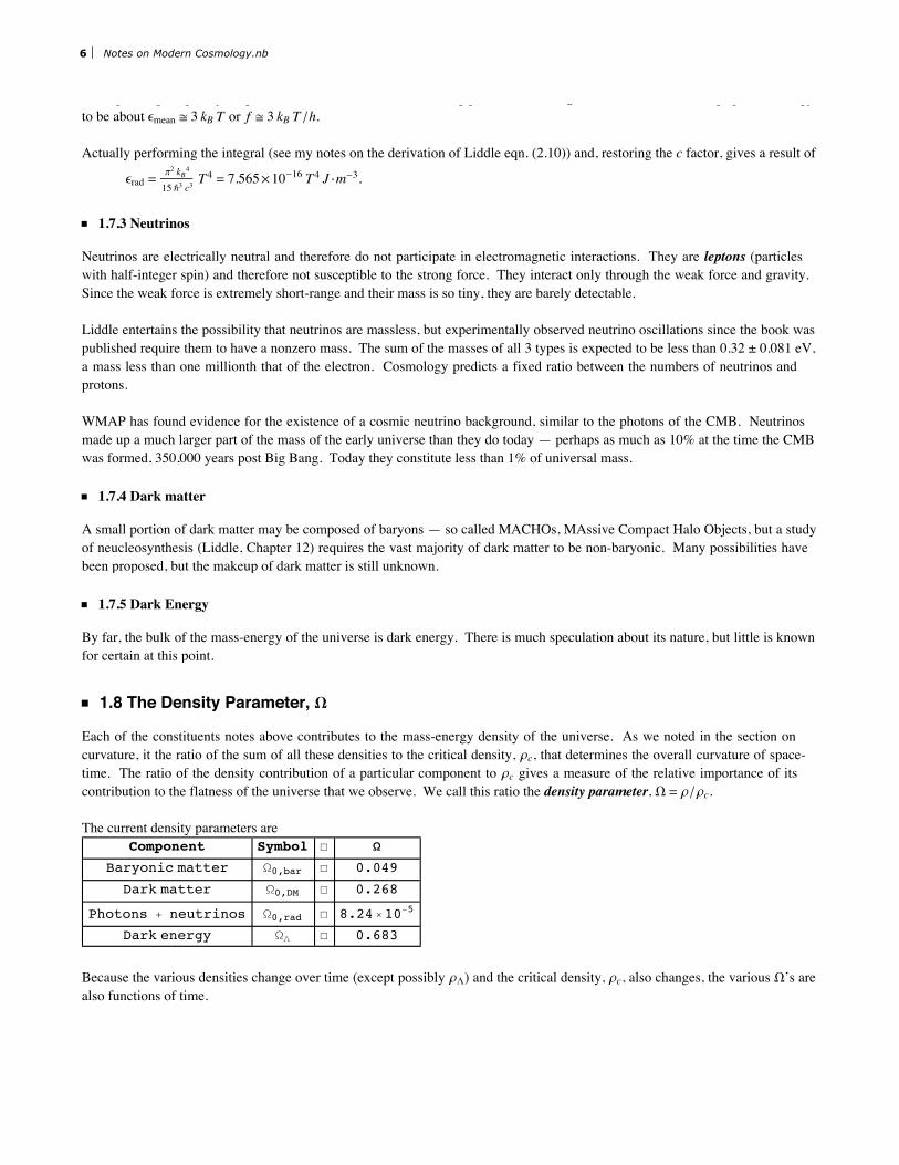
The integrand is the famous black-body spectrum:

PlotA9y3 ë HExp@yD - 1L=, 8y, 0, 12<, AxesLabel Ø 9"y=eêkBT", "y3êHey-1L"=E

2 4 6 8 10 12y=eêkBT

0.2

0.4

0.6

0.8

1.0

1.2

1.4

y3êHey-1L

The area under any segment of this curve from y to y + dy, when multiplied by 8 pHkB TL4

h3, gives the energy density within the

corresponding frequency range. Since this distribution has a strong peak at e = 2.82 kB T , we can take the average photon energyto be about emean @ 3 kB T or f @ 3 kB T êh.

Actually performing the integral (see my notes on the derivation of Liddle eqn. (2.10)) and, restoring the c factor, gives a result of

erad =p2 kB4

15 —3 c3T4 = 7.565µ10-16 T4 J ÿm-3.


The area under any segment of this curve from y to y + dy, when multiplied by 8 pHkB TL4

h3, gives the energy density within the

corresponding frequency range. Since this distribution has a strong peak at e = 2.82 kB T , we can take the average photon energyto be about emean @ 3 kB T or f @ 3 kB T êh.

Actually performing the integral (see my notes on the derivation of Liddle eqn. (2.10)) and, restoring the c factor, gives a result of

erad =p2 kB4

15 —3 c3T4 = 7.565µ10-16 T4 J ÿm-3.

ü 1.7.3 Neutrinos

Neutrinos are electrically neutral and therefore do not participate in electromagnetic interactions. They are leptons (particleswith half-integer spin) and therefore not susceptible to the strong force. They interact only through the weak force and gravity.Since the weak force is extremely short-range and their mass is so tiny, they are barely detectable.

Liddle entertains the possibility that neutrinos are massless, but experimentally observed neutrino oscillations since the book waspublished require them to have a nonzero mass. The sum of the masses of all 3 types is expected to be less than 0.32 ± 0.081 eV,a mass less than one millionth that of the electron. Cosmology predicts a fixed ratio between the numbers of neutrinos andprotons.

WMAP has found evidence for the existence of a cosmic neutrino background, similar to the photons of the CMB. Neutrinosmade up a much larger part of the mass of the early universe than they do today — perhaps as much as 10% at the time the CMBwas formed, 350,000 years post Big Bang. Today they constitute less than 1% of universal mass.

ü 1.7.4 Dark matter

A small portion of dark matter may be composed of baryons — so called MACHOs, MAssive Compact Halo Objects, but a studyof neucleosynthesis (Liddle, Chapter 12) requires the vast majority of dark matter to be non-baryonic. Many possibilities havebeen proposed, but the makeup of dark matter is still unknown.

ü 1.7.5 Dark Energy

By far, the bulk of the mass-energy of the universe is dark energy. There is much speculation about its nature, but little is knownfor certain at this point.

ü 1.8 The Density Parameter, W

Each of the constituents notes above contributes to the mass-energy density of the universe. As we noted in the section oncurvature, it the ratio of the sum of all these densities to the critical density, rc, that determines the overall curvature of space-time. The ratio of the density contribution of a particular component to rc gives a measure of the relative importance of itscontribution to the flatness of the universe that we observe. We call this ratio the density parameter, W= r ê rc.

The current density parameters areComponent Symbol Ñ W

Baryonic matter W0,bar Ñ 0.049

Dark matter W0,DM Ñ 0.268

Photons + neutrinos W0,rad Ñ 8.24ä10-5

Dark energy WL Ñ 0.683

Because the various densities change over time (except possibly rL) and the critical density, rc, also changes, the various W’s arealso functions of time.


ü 1.8 The Cosmological Constant, L

Because all matter-energy is gravitationally attractive, there are no solutions in GR that represent a static, homogeneous universe.What is needed is something that exerts an outward pressure to keep the whole thing from collapsing. We will see that introduc-ing a “cosmological constant,” L, that may or may not actually be constant, can offset this collapse and lead to the acceleratingexpansion that we see today. As in the table above, we can define a density parameter associated with L, called WL =

rLrc

L

3H2.

Note that, though L may be a constant, WL is not. A universe in which WL = 1 is known as a deSitter universe and is theultimate fate of our universe.

The mass density, r, is what we usually think of as a density - the amount of a substance contained in a unit volume. But, sinceL is a quality of spacetime and not a substance, rL is somewhat more difficult to visualize. It is helpful to think of L is as a fluidthat fills spacetime and has an energy density rL and exerts a pressure, pL = -rL c2. Since rL is a positive constant, the cosmo-logical constant exerts a constant outward pressure. It is this pressure that is the source of the current accelerating expansion ofthe universe.

2 General RelativityLiddle, for the most part, avoids GR, relegating it to an “advanced topic” chapter and only covering it there with a broad brush. Ithink that, since cosmology has its roots firmly in the soil of GR, it’s a good idea to dig a bit deeper. The following is still at apretty descriptive level, but may help to establish a few important concepts.

ü 2.1 The Metric Tensor

We are so accustomed to flat space that we automatically think in those terms, where the separation between objects, ds, is givenby the Euclidean metric, ds2 = dx2 + dy2 + dz2 in Cartesian coordinates. In the notation of relativity, this is written asds2 = dij dxi dx j. This simple-looking expression includes four important GR conventions/constructs:

1) Roman letter indices indicate 1, 2, and 3. (Greek letter indices are used to stand for 0, 1, 2, and 3.)2) The common spatial axis designations, x, y, and z, are replaced by x1, x2, and x3, summarized as xi or x j. Note that i

and j are indices, not powers. (When Greek indices are used this correspondence remains, and additionally, x0 stands for time, t,or more correctly, ct.)

3) Einstein summation applies, in which a sum over repeated indices is assumed. Since i and j appear twice each on theright hand side, a sum over them as they run from 1 to 3 is implied. So, writing the metric in its full expression,ds2 =⁄i=1

3 ⁄ j=13 dij dxi dx j. (The same summation convention applies to Greek indices, except that they run from 0 to 3.)

4) d is the Kronecker delta; dij = 1 if i = j and dij = 0 otherwise. In this application, dij can be thought of as a rank-2 (2indices) metric tensor, a 3×3 matrix indexed by i and j that specifies coefficients for each of the nine products in the above sums.Generally the metric tensor is much more complicated, but from the previous definition of dij we can see that in this case it’s justthe identity matrix:

AdijE =

1 0 00 1 00 0 1

.

In special relativity, (SR), we deal with frames of reference that are stationary or moving at a constant velocity with respect toeach other. These are called inertial frames or Lorentz frames. Analysis of these reference frames shows that our intuitiveconcept of separate time and space coordinates leads to wrong conclusions at high relative velocities and we must “weld” themtogether into the a “spacetime continuum.” Hence the need for Greek indices that run over the 4 dimensions of space and time.Now we write the above metric as ds2 = hab dxa dxb, using Greek indices a and b to indicate 4 values for the 4 dimensions. Herehab is the Minkowski metric tensor for flat spacetime. It too is simple:

AhabE =

1 0 0 00 -1 0 00 0 -1 00 0 0 -1

.

Note though, that the time component now has a different sign from the spatial ones, so the Einstein summation could result in anegative value for ds2. (The Euclidean metric is always non-negative.)

[Note also that this definition and some of the following equations differ from those in Liddle’s book by a minus sign. Thisdifference reflects my preference for the so called “mostly minus metric” in contrast to Liddle’s use of the “mostly plus metric.”Thus, Liddle would write,

AhabE =

-1 0 0 00 1 0 00 0 1 00 0 0 1

.

Unfortunately, there is not a single convention for this and it’s one of those annoying complications in physics that just makealready difficult concepts a little bit more confusing. Sorry about that, but I’m writing this for me, so I get to do it the way I’mmost comfortable!]

In SR, spacetime is always flat — the Minkowski metric always applies. In GR, though, we no longer have the guarantee of thecomforting normalcy of flat spacetime. Not surprisingly, this means that the metric tensor can be much more complicated. Nowwe write the metric as, ds2 = gmn dxm dxn. (We could still use a and b, but m and n are conventional.) This new metric tensor, gmn,now stands for any general metric tensor, even ones that apply to curved spacetime. The cosmological principle, though, allowsus to limit the ones that concern us by requiring that, neglecting local variations, spacetime must have the same curvatureeverywhere.

The simplest of these cases is the Friedmann-Lemaître-Robertson-Walker (FLRW) metric tensor for an expanding, flat space-time. As you can probably guess, this is just,

gmnFLRW =

1 0 0 00 -a2 HtL 0 00 0 -a2 HtL 00 0 0 -a2 HtL

.

So far, we have worked in Cartesian coordinates, but, since we are looking radially outward from earth, spherical spatial coordi-nates (r, q, f) are more natural. If we incorporate these and construct a general metric for a curved, expanding spacetime, we getthe Robertson-Walker (RW) metric,

dsRW2 = c2 dt2 - a2HtLB dr2

1-kr2+ r2Id q2 + sin2 q d f2MF.

The spacetime described by this metric is the most general one that is both homogeneous and isotropic. The time coordinate,called cosmic time, is the time of a fundamental observer whose only motion is due to the expansion or contraction of space-time. The spatial coordinates (r, q and f) assigned by a fundamental observer are comoving coordinates and, at any specificcosmic time, all fundamental observers will be measuring the same 3-dimensional space-like hypersurface embedded in 4-dimensional spacetime. Each such hypersurface represents all of space at that moment of cosmic time. It can be thought of in a3-dimensional analogy as the 2-dimensional surface that is formed by the events corresponding to the same instant in cosmictime on the diverging world lines of all fundamental observers in expanding spacetime.

We would like to know how such a spacetime evolves, since that will contain important clues to the evolution of our ownuniverse. This evolution is specified by the field equations of GR. So, let’s take a brief detour to understand those fieldequations.








AdijE =

1 0 00 1 00 0 1

.


AhabE =

1 0 0 00 -1 0 00 0 -1 00 0 0 -1

.



AhabE =

-1 0 0 00 1 0 00 0 1 00 0 0 1

.




gmnFLRW =

1 0 0 00 -a2 HtL 0 00 0 -a2 HtL 00 0 0 -a2 HtL

.













AdijE =

1 0 00 1 00 0 1

.


AhabE =

1 0 0 00 -1 0 00 0 -1 00 0 0 -1

.



AhabE =

-1 0 0 00 1 0 00 0 1 00 0 0 1

.




gmnFLRW =

1 0 0 00 -a2 HtL 0 00 0 -a2 HtL 00 0 0 -a2 HtL

.






ü 2.2 Curvature

We start with some definitions. We call a smoothly curved space that is everywhere locally flat, a manifold. The surface of asphere, for example is a manifold — small parts of it look flat. The surface of a cone is not a manifold, since, no matter howclosely you look, its apex is not flat. The curved spacetime of GR is a manifold, but it’s a manifold with two additional proper-ties:

1) It’s differentiable. Almost all spaces that concern physicists are differentiable, since that provides some vitallyimportant characteristics and seems, thankfully, to be the way nature operates.

2) Its metric tensor must be symmetric (ie, gmn = gnm).

Such manifolds are called Riemann manifolds. They were first studied in depth by Bernhard Riemann in the mid 19th-century.(Actually, the manifolds of GR are pseudo-Riemann manifolds, since they can have, as noted above, a positive, zero or negativeds2.) Riemann was able to show that he could capture all curvature information about these manifolds in a rank-4 tensor calledthe Riemann curvature tensor, Rbgd

a . Rbgda = 0 implies a flat manifold.

GR doesn’t actually use the full Rbgda , but instead uses two other measures of curvature derived from it. A tensor can have its

rank lowered by a process called contraction that amounts to multiplying it by another tensor with the same index in the oppositeposition (up or down). [Think of turning a vector (a rank-1 tensor) into a scalar (a rank-0 tensor) by forming a dot product withanother vector.] When the first and last indices of the Riemann curvature tensor are contracted, the result is the rank-2 Riccitensor, Rmn. Another contraction over the remaining two indices results in the Ricci scalar, R = gij Rij. Einstein then collected

these two entities into one — the Einstein tensor, Gmn = Rmn -12

R gmn.

The Einstein field equations relate the curvature of spacetime to the configuration of mass-energy that causes the curvature. Wehave seen that curvature is captured in the Einstein tensor, but we need a way to describe the energy and momentum of thecollection of particles whose gravity is the source of the curvature. The answer is T mn, the symmetric, rank-2 energy-momentumtensor (sometimes called the “stress-energy tensor”). Consider a collection of particles moving along their individual worldlines. Each carries its four-momentum (a combination of energy and momentum) with it, and the collection forms a “river offour-momentum” flowing through spacetime. The density and flow of this river is the source of the general relativistic gravita-tional field and is captured in T mn.

The Einstein field equations then relate Gmn to Tmn in the famous expression, Gmn = - 8 pGc4

Tmn. This is often written in

“geometrized” units, where 8 p G = c = 1, as the frustratingly obscure Gmn = - Tmn. This equation relates two symmetric 4×4matrices, thus representing, at most, 10 independent equations (symmetry requirements eliminate 6 of the 4×4=16 equations).There are, however, two important special cases that, because of their symmetries, significantly reduce this number. These are:

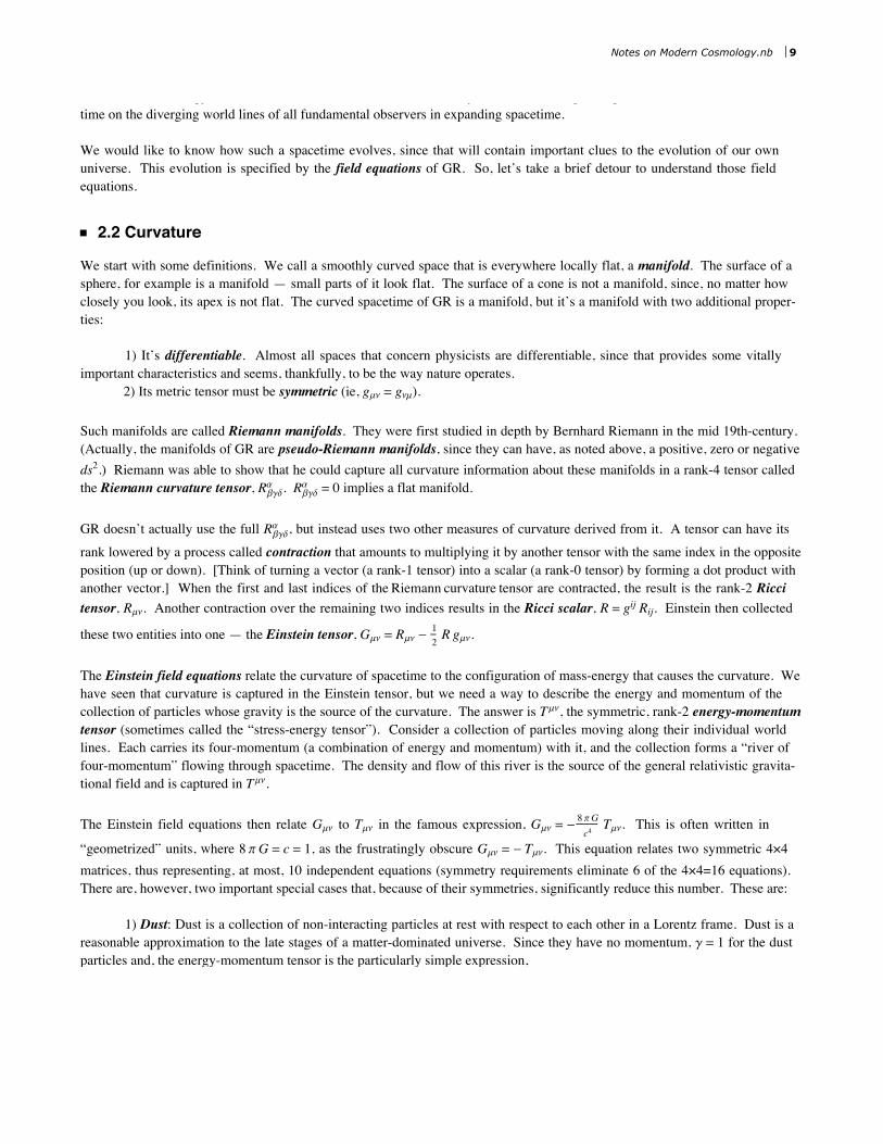
1) Dust: Dust is a collection of non-interacting particles at rest with respect to each other in a Lorentz frame. Dust is areasonable approximation to the late stages of a matter-dominated universe. Since they have no momentum, g = 1 for the dustparticles and, the energy-momentum tensor is the particularly simple expression,

ATDustmn

E =

rc2 0 0 00 0 0 00 0 0 00 0 0 0

, where mass density r = n m, with n being the number density of the particles.

The field equations for dust become a single equation.

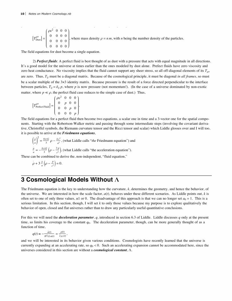
2) Perfect fluids: A perfect fluid is best thought of as dust with a pressure that acts with equal magnitude in all directions.It’s a good model for the universe at times earlier than the ones modeled by dust alone. Prefect fluids have zero viscosity andzero heat conductance. No viscosity implies that the fluid cannot support any sheer stress, so all off-diagonal elements of its Tmn

are zero. Thus, Tij must be a diagonal matrix. Because of the cosmological principle, it must be diagonal in all frames, so mustbe a scalar multiple of the 3×3 identity matrix. Because pressure is the result of a force directed perpendicular to the interfacebetween particles, Tij = dij p, where p is now pressure (not momentum!). (In the case of a universe dominated by non-exoticmatter, where p ` r, the perfect fluid case reduces to the simple case of dust.) Thus,

ATPerfect Fluidmn

E =

rc2 0 0 00 p 0 00 0 p 00 0 0 p

.

The field equations for a perfect fluid then become two equations, a scalar one in time and a 3-vector one for the spatial compo-nents. Starting with the Robertson-Walker metric and passing through some intermediate steps (involving the covariant deriva-tive, Christoffel symbols, the Riemann curvature tensor and the Ricci tensor and scalar) which Liddle glosses over and I will too,it is possible to arrive at the Friedmann equations,

Kaÿ

aO2= 8 pG

3r - k c2

a2, (what Liddle calls “the Friedmann equation”) and

aÿÿ

a= - 4 pG

3Jr -

3 pc2N, (what Liddle calls “the acceleration equation”).

These can be combined to derive the, non-independent, “fluid equation,”

rÿ+ 3 aÿ

aJr -

p

c2N = 0.


We start with some definitions. We call a smoothly curved space that is everywhere locally flat, a manifold. The surface of asphere, for example is a manifold — small parts of it look flat. The surface of a cone is not a manifold, since, no matter howclosely you look, its apex is not flat. The curved spacetime of GR is a manifold, but it’s a manifold with two additional proper-ties:

1) It’s differentiable. Almost all spaces that concern physicists are differentiable, since that provides some vitallyimportant characteristics and seems, thankfully, to be the way nature operates.

2) Its metric tensor must be symmetric (ie, gmn = gnm).

Such manifolds are called Riemann manifolds. They were first studied in depth by Bernhard Riemann in the mid 19th-century.(Actually, the manifolds of GR are pseudo-Riemann manifolds, since they can have, as noted above, a positive, zero or negativeds2.) Riemann was able to show that he could capture all curvature information about these manifolds in a rank-4 tensor calledthe Riemann curvature tensor, Rbgd

a . Rbgda = 0 implies a flat manifold.

GR doesn’t actually use the full Rbgda , but instead uses two other measures of curvature derived from it. A tensor can have its

rank lowered by a process called contraction that amounts to multiplying it by another tensor with the same index in the oppositeposition (up or down). [Think of turning a vector (a rank-1 tensor) into a scalar (a rank-0 tensor) by forming a dot product withanother vector.] When the first and last indices of the Riemann curvature tensor are contracted, the result is the rank-2 Riccitensor, Rmn. Another contraction over the remaining two indices results in the Ricci scalar, R = gij Rij. Einstein then collected

these two entities into one — the Einstein tensor, Gmn = Rmn -12

R gmn.

The Einstein field equations relate the curvature of spacetime to the configuration of mass-energy that causes the curvature. Wehave seen that curvature is captured in the Einstein tensor, but we need a way to describe the energy and momentum of thecollection of particles whose gravity is the source of the curvature. The answer is T mn, the symmetric, rank-2 energy-momentumtensor (sometimes called the “stress-energy tensor”). Consider a collection of particles moving along their individual worldlines. Each carries its four-momentum (a combination of energy and momentum) with it, and the collection forms a “river offour-momentum” flowing through spacetime. The density and flow of this river is the source of the general relativistic gravita-tional field and is captured in T mn.

The Einstein field equations then relate Gmn to Tmn in the famous expression, Gmn = - 8 pGc4

Tmn. This is often written in

“geometrized” units, where 8 p G = c = 1, as the frustratingly obscure Gmn = - Tmn. This equation relates two symmetric 4×4matrices, thus representing, at most, 10 independent equations (symmetry requirements eliminate 6 of the 4×4=16 equations).There are, however, two important special cases that, because of their symmetries, significantly reduce this number. These are:

1) Dust: Dust is a collection of non-interacting particles at rest with respect to each other in a Lorentz frame. Dust is areasonable approximation to the late stages of a matter-dominated universe. Since they have no momentum, g = 1 for the dustparticles and, the energy-momentum tensor is the particularly simple expression,

ATDustmn

E =

rc2 0 0 00 0 0 00 0 0 00 0 0 0

, where mass density r = n m, with n being the number density of the particles.

The field equations for dust become a single equation.

2) Perfect fluids: A perfect fluid is best thought of as dust with a pressure that acts with equal magnitude in all directions.It’s a good model for the universe at times earlier than the ones modeled by dust alone. Prefect fluids have zero viscosity andzero heat conductance. No viscosity implies that the fluid cannot support any sheer stress, so all off-diagonal elements of its Tmn

are zero. Thus, Tij must be a diagonal matrix. Because of the cosmological principle, it must be diagonal in all frames, so mustbe a scalar multiple of the 3×3 identity matrix. Because pressure is the result of a force directed perpendicular to the interfacebetween particles, Tij = dij p, where p is now pressure (not momentum!). (In the case of a universe dominated by non-exoticmatter, where p ` r, the perfect fluid case reduces to the simple case of dust.) Thus,

ATPerfect Fluidmn

E =

rc2 0 0 00 p 0 00 0 p 00 0 0 p

.

The field equations for a perfect fluid then become two equations, a scalar one in time and a 3-vector one for the spatial compo-nents. Starting with the Robertson-Walker metric and passing through some intermediate steps (involving the covariant deriva-tive, Christoffel symbols, the Riemann curvature tensor and the Ricci tensor and scalar) which Liddle glosses over and I will too,it is possible to arrive at the Friedmann equations,

Kaÿ

aO2= 8 pG

3r - k c2

a2, (what Liddle calls “the Friedmann equation”) and

aÿÿ

a= - 4 pG

3Jr -

3 pc2N, (what Liddle calls “the acceleration equation”).

These can be combined to derive the, non-independent, “fluid equation,”

rÿ+ 3 aÿ

aJr -

p

c2N = 0.

3 Cosmological Models Without LThe Friedmann equation is the key to understanding how the curvature, k, determines the geometry, and hence the behavior, ofthe universe. We are interested in how the scale factor, aHtL, behaves under these different scenarios. As Liddle points out, k isoften set to one of only three values, ±1 or 0. The disadvantage of this approach is that we can no longer set a0 = 1. This is aserious limitation. In this section, though, I will set k to only those values because my purpose is to explore qualitatively thebehavior of open, closed and flat universes rather than to draw any particularly useful quantitative conclusions.

For this we will need the deceleration parameter, q, introduced in section 6.3 of Liddle. Liddle discusses q only at the presenttime, so limits his coverage to the constant q0. The deceleration parameter, though, can be more generally thought of as afunction of time,

qHtL ª - aÿÿHtLH2HtL aHtL

=rHtL2 rcHtL

,

and we will be interested in its behavior given various conditions. Cosmologists have recently learned that the universe iscurrently expanding at an accelerating rate, so q0 < 0. Such an accelerating expansion cannot be accommodated here, since theuniverses considered in this section are without a cosmological constant, L.


ü 3.1 Characteristics of Flat Universes

We first examine the properties of flat matter-dominated and radiation-dominated universes without a cosmological constant(dark energy), and then tabulate their behavior for other curvatures.

ü 3.1.1 The Flat Non-relativistic Matter-dominated Universe

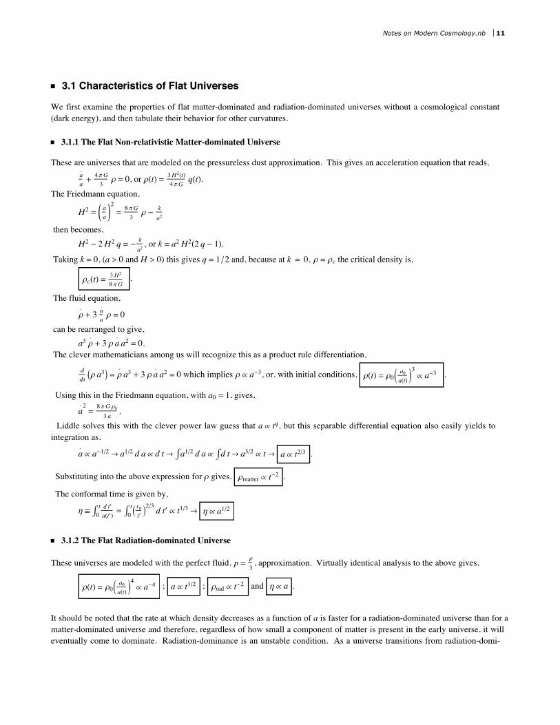
These are universes that are modeled on the pressureless dust approximation. This gives an acceleration equation that reads,aÿÿ

a+ 4 pG

3r = 0, or rHtL = 3H2HtL

4 pGqHtL.

The Friedmann equation,

H2 = Kaÿ

aO2= 8 pG

3r - k

a2

then becomes, H2 - 2 H2 q = - k

a2, or k = a2 H2H2 q - 1L.

Taking k = 0, Ha > 0 and H > 0) this gives q = 1 ê2 and, because at k = 0, r = rc the critical density is,

rcHtL =3H2

8 pG.

The fluid equation,

rÿ+ 3 aÿ

ar = 0

can be rearranged to give, a3 r

ÿ+ 3 r a

ÿa2 = 0.

The clever mathematicians among us will recognize this as a product rule differentiation,

„

„tIr a3M = r

ÿa3 + 3 r a

ÿa2 = 0 which implies r µ∝ a-3, or, with initial conditions, rHtL = r0J

a0aHtL

N3µ∝ a-3 .

Using this in the Friedmann equation, with a0 = 1, gives,

aÿ 2=8 pG r03 a

. Liddle solves this with the clever power law guess that a µ∝ tq, but this separable differential equation also easily yields tointegration as,

aÿµ∝ a-1ê2 Ø a1ê2 d a µ∝ d t Ø Ÿ a1ê2 d a µ∝ Ÿ d t Ø a3ê2 µ∝ t Ø a µ∝ t2ê3 .

Substituting into the above expression for r gives, rmatter µ∝ t-2 .

The conformal time is given by,

h ª Ÿ0t d t£

aHt£L= Ÿ0

tIt 0t£M2ê3 d t£ µ∝ t1ê3 Ø h µ∝ a1ê2

ü 3.1.2 The Flat Radiation-dominated Universe

These universes are modeled with the perfect fluid, p =r

3, approximation. Virtually identical analysis to the above gives,

rHtL = r0Ja0aHtL

N4µ∝ a-4 ; a µ∝ t1ê2 ; rrad µ∝ t-2 and h µ∝ a .

It should be noted that the rate at which density decreases as a function of a is faster for a radiation-dominated universe than for amatter-dominated universe and therefore, regardless of how small a component of matter is present in the early universe, it willeventually come to dominate. Radiation-dominance is an unstable condition. As a universe transitions from radiation-domi-nance to matter-dominance, the expansion rate will speed up from a

ÿµ∝ t-1ê2 to a

ÿµ∝ t-1ê3.


These universes are modeled with the perfect fluid, p =r

3, approximation. Virtually identical analysis to the above gives,

rHtL = r0Ja0aHtL

N4µ∝ a-4 ; a µ∝ t1ê2 ; rrad µ∝ t-2 and h µ∝ a .

It should be noted that the rate at which density decreases as a function of a is faster for a radiation-dominated universe than for amatter-dominated universe and therefore, regardless of how small a component of matter is present in the early universe, it willeventually come to dominate. Radiation-dominance is an unstable condition. As a universe transitions from radiation-domi-nance to matter-dominance, the expansion rate will speed up from a

ÿµ∝ t-1ê2 to a

ÿµ∝ t-1ê3.

ü 3.2 Specific Solutions Based on Curvature

The following tables give the evolution of the scale factor for matter- and radiation-dominated universes for each of the threecanonical curvatures, k = 0, ±1. Because our universe appears to be flat to a high degree of certainty and dominated by acosmological constant, none of these solutions is of more than theoretical interest, so I will just tabulate the results rather thanderive them.

Matter-dominated UniversesCharacteristics for all h for small hk q0 a t a HhL t a HtL

0 = 1 ê 2 H6 p G r0L1ê3 t2ê3 - - - µ∝ t2ê3

+1 > 1 ê 2 Jq0

2 q0-1N H1 - cos hL J

q02 q0-1

N Hh - sin hL µ∝ h2 µ∝ h3 µ∝ t2ê3

-1 < 1 ê 2 Jq0

1-2 q0N Hcosh h - 1L J

q01-2 q0

N Hsinh h - hL µ∝ h2 µ∝ h3 µ∝ t2ê3

Radiation-dominated UniversesCharacteristics for all h for small hk q0 a t a HhL t a HtL

0 = 1 ê 2 I32 p G r0

3M1ê4

t1ê2 - - - µ∝ t1ê2

+1 > 1 ê 2 2 q02 q0-1

Hsin hL2 q02 q0-1

H1 - cos hL µ∝ h µ∝ h2 µ∝ t1ê2

-1 < 1 ê 2 2 q01-2 q0

Hsinh hL2 q0

1-2 q0Hcosh h - hL µ∝ h µ∝ h2 µ∝ t1ê2

ü 3.3 Particle Number Density

We have been concerned so far with mass-energy density, r, but another useful density, number density, n, simply counts thenumber of particles of a particular type in a unit volume. It’s useful because a system at thermal equilibrium will statisticallypreserve the number of each type of particle, since, by definition, equilibrium reactions that produce or destroy particles run atthe same rate in both directions. Number density will change in an expanding universe, though, because expansion changes thevolume, so, n µ∝ a-3.

This relation is exactly what we would expect for non-relativistic matter (rmatter µ∝ a-3), but we have seen that radiation energydensity falls off more quickly (rrad µ∝ a-4). The extra factor of a-1 is due to the loss of energy by the photons as their wave-lengths are stretched in the expansion. So, even though energy densities of matter and radiation evolve differently in an expand-ing universe, their number densities evolve in exactly the same way, n µ∝ a-3.

4 Cosmological Models With L

ü 4.1 The Cosmological Constant

Einstein quickly realized that, if the energy sources in the energy-momentum tensor are only matter Hpmat = 0) and radiationIprad = rrad c2 ë3), there are no solutions to the field equations of GR that describe a static, homogeneous universe. To remedythis situation and bring GR into alignment with the astronomical thinking of the day, he proposed including a “cosmologicalconstant,” L, HpL = -rL) so that his field equations now read Rmn -

12

R gmn + L gmn = - 8 pGc4

Tmn. The Friedmann equation that

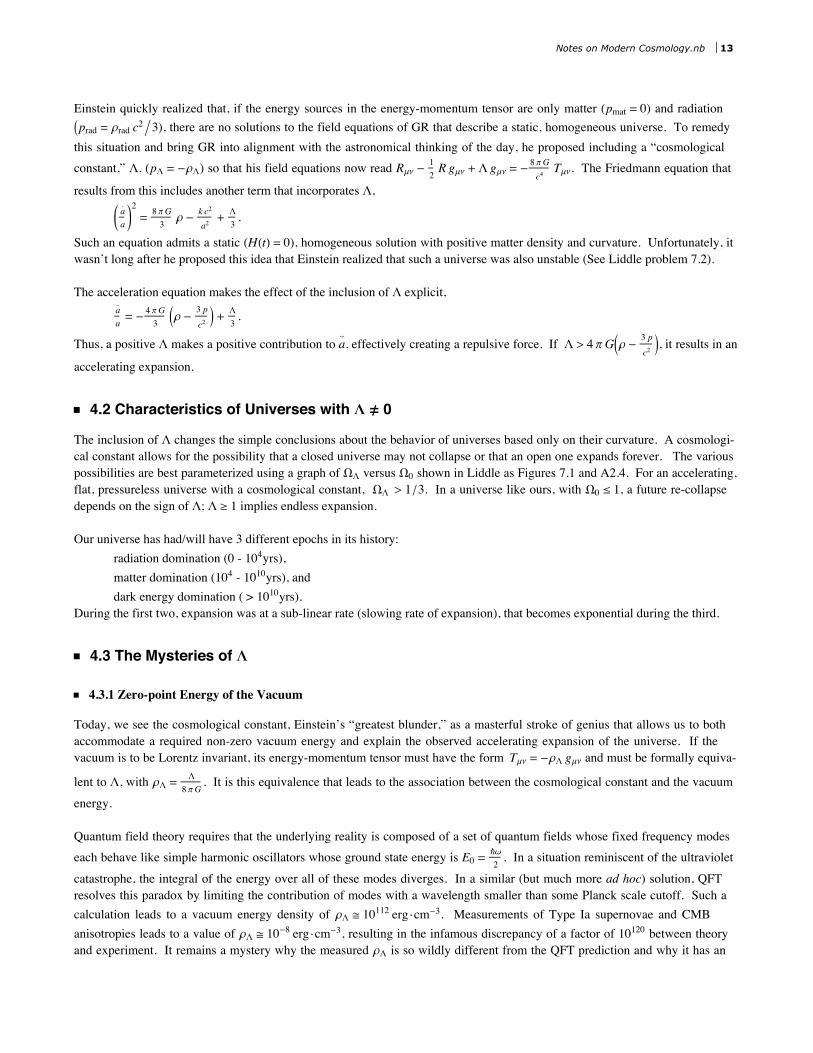
results from this includes another term that incorporates L,

Kaÿ

aO2= 8 pG

3r - k c2

a2+ L

3.

Such an equation admits a static HHHtL = 0), homogeneous solution with positive matter density and curvature. Unfortunately, itwasn’t long after he proposed this idea that Einstein realized that such a universe was also unstable (See Liddle problem 7.2).

The acceleration equation makes the effect of the inclusion of L explicit,aÿÿ

a= - 4 pG

3Jr -

3 pc2N + L

3.

Thus, a positive L makes a positive contribution to aÿÿ, effectively creating a repulsive force. If L > 4 p GJr -

3 pc2N, it results in an

accelerating expansion.


Einstein quickly realized that, if the energy sources in the energy-momentum tensor are only matter Hpmat = 0) and radiationIprad = rrad c2 ë3), there are no solutions to the field equations of GR that describe a static, homogeneous universe. To remedythis situation and bring GR into alignment with the astronomical thinking of the day, he proposed including a “cosmologicalconstant,” L, HpL = -rL) so that his field equations now read Rmn -

12

R gmn + L gmn = - 8 pGc4

Tmn. The Friedmann equation that

results from this includes another term that incorporates L,

Kaÿ

aO2= 8 pG

3r - k c2

a2+ L

3.

Such an equation admits a static HHHtL = 0), homogeneous solution with positive matter density and curvature. Unfortunately, itwasn’t long after he proposed this idea that Einstein realized that such a universe was also unstable (See Liddle problem 7.2).

The acceleration equation makes the effect of the inclusion of L explicit,aÿÿ

a= - 4 pG

3Jr -

3 pc2N + L

3.

Thus, a positive L makes a positive contribution to aÿÿ, effectively creating a repulsive force. If L > 4 p GJr -

3 pc2N, it results in an

accelerating expansion.

ü 4.2 Characteristics of Universes with L ¹≠ 0

The inclusion of L changes the simple conclusions about the behavior of universes based only on their curvature. A cosmologi-cal constant allows for the possibility that a closed universe may not collapse or that an open one expands forever. The variouspossibilities are best parameterized using a graph of WL versus W0 shown in Liddle as Figures 7.1 and A2.4. For an accelerating,flat, pressureless universe with a cosmological constant, WL > 1 ê3. In a universe like ours, with W0 § 1, a future re-collapsedepends on the sign of L; L ¥ 1 implies endless expansion.

Our universe has had/will have 3 different epochs in its history:radiation domination (0 - 104yrs),matter domination (104 - 1010yrs), anddark energy domination ( > 1010yrs).

During the first two, expansion was at a sub-linear rate (slowing rate of expansion), that becomes exponential during the third.

ü 4.3 The Mysteries of L

ü 4.3.1 Zero-point Energy of the Vacuum

Today, we see the cosmological constant, Einstein’s “greatest blunder,” as a masterful stroke of genius that allows us to bothaccommodate a required non-zero vacuum energy and explain the observed accelerating expansion of the universe. If thevacuum is to be Lorentz invariant, its energy-momentum tensor must have the form Tmn = -rL gmn and must be formally equiva-

lent to L, with rL = L

8 pG. It is this equivalence that leads to the association between the cosmological constant and the vacuum

energy.

Quantum field theory requires that the underlying reality is composed of a set of quantum fields whose fixed frequency modeseach behave like simple harmonic oscillators whose ground state energy is E0 =

—w

2. In a situation reminiscent of the ultraviolet

catastrophe, the integral of the energy over all of these modes diverges. In a similar (but much more ad hoc) solution, QFTresolves this paradox by limiting the contribution of modes with a wavelength smaller than some Planck scale cutoff. Such acalculation leads to a vacuum energy density of rL @ 10112 erg ÿcm-3. Measurements of Type Ia supernovae and CMBanisotropies leads to a value of rL @ 10-8 erg ÿcm-3, resulting in the infamous discrepancy of a factor of 10120 between theoryand experiment. It remains a mystery why the measured rL is so wildly different from the QFT prediction and why it has anexceedingly small, but non-zero, value.


Today, we see the cosmological constant, Einstein’s “greatest blunder,” as a masterful stroke of genius that allows us to bothaccommodate a required non-zero vacuum energy and explain the observed accelerating expansion of the universe. If thevacuum is to be Lorentz invariant, its energy-momentum tensor must have the form Tmn = -rL gmn and must be formally equiva-

lent to L, with rL = L

8 pG. It is this equivalence that leads to the association between the cosmological constant and the vacuum

energy.

Quantum field theory requires that the underlying reality is composed of a set of quantum fields whose fixed frequency modeseach behave like simple harmonic oscillators whose ground state energy is E0 =

—w

2. In a situation reminiscent of the ultraviolet

catastrophe, the integral of the energy over all of these modes diverges. In a similar (but much more ad hoc) solution, QFTresolves this paradox by limiting the contribution of modes with a wavelength smaller than some Planck scale cutoff. Such acalculation leads to a vacuum energy density of rL @ 10112 erg ÿcm-3. Measurements of Type Ia supernovae and CMBanisotropies leads to a value of rL @ 10-8 erg ÿcm-3, resulting in the infamous discrepancy of a factor of 10120 between theoryand experiment. It remains a mystery why the measured rL is so wildly different from the QFT prediction and why it has anexceedingly small, but non-zero, value.

ü 4.3.2 Why are WL and Wmat of Roughly the Same Size?

If we lump dark matter with ordinary baryonic matter, the matter and dark energy density parameters are, Wmat @ 0.3 andWL @ 0.7. Since rmat µ∝ a-3HtL and rL µ∝ a0HtL, this near equality of density parameters exists for a very small portion of thehistory of the universe. It appears that the transition from a matter-dominated to a cosmological constant-dominated universe,with its inherent accelerated expansion, is a relatively recent phenomenon. Why we happen to live during this particular periodin the history of the universe also seems to demand an explanation. There is no consensus on an answer.

ü 4.4 Some Possible Solutions

Over the last decade and a half, almost everyone in the field of cosmology has come to accept the model of a universe expandingat an accelerating rate with Wmat @ 0.3 and WL @ 0.7. There are a few holdouts who continue to support a model of unacceleratedexpansion with Wmat @ 1, but these theories, all involving various forms of invalidation of high-redshift observational data, seemincreasingly contrived and untenable. Assuming that the accelerated expansion is real, there are several possible ways out of theconundrum.

ü 4.4.1 Failure of GR

If we accept that we live in an accelerating, isotropic and homogeneous universe, GR in its current form is unambiguously clearthat some source of negative pressure (“dark energy” for lack of a better term) is required. A dark energy-free acceleration canarise and the observed universe can be postdicted by requiring a modification of GR at cosmic scales.

Some string theorists have proposed ideas of this sort that require modifications of the Friedmann equation. I don’t understandthese ideas very well, but they seem to require gravity to be four-dimensional below a certain (very large) length scale and higher-dimensional above it.

Others have proposed four-dimensional modifications to GR at all scales. In an elegant approach similar to Feynman’s pathintegral formulation of QM, the Einstein field equations can be derived by minimizing an action given by the spacetime integralof the Ricci curvature scalar, R,

S = Ÿ d4 x gmn R.

Theorists proposing a modification to GR that does not require the additional dimensions of string theory, simply add a 1 êR-dependent term to the integrand,

S = ‡ d4 x gmn JR -m4

RN, where m is a tunable parameter.

These theories admit accelerating solutions, but make other predictions that appear to conflict with observations.

Unfortunately, all of these approaches to modifying GR lead to some fine-tuning mysteries of their own and, to my untrainedeye, seem to add complexity (and probably inconsistencies with observation) without really solving the underlying problemsinherent in the accelerating expansion.

ü 4.4.2 Varying L

The Friedmann equation with L requires that aÿ 2µ∝ a2 r + constant. So, for acceleration to occur, the dark energy density must

fall off more slowly than a-2. Neither matter (rmat µ∝ a-3) nor radiation (rrad µ∝ a-4) does the job. A constant L (rL = constant)will work, but so will a slowly decreasing L. It offers a potential solution to the problem of a small but non-zero cosmologicalconstant: L has been decreasing for a long time, falling asymptotically toward zero, and we happen to live at the time when it hasits current tiny value. It is possible that the problem of the close values of Wmat and WL might also be resolved in this way.

The simplest of these possibilities is a scalar inflaton field dropping slowly in a weak potential field. (If the potential werestronger, L would presumably have already reached its minimum.) This can be thought of as a “quintessence fluid” with anequation of state given by, pQ = w rQ c2, where w is a constant. The w = -1 case is the familiar cosmological constant, withexpansion occurring for w < -1 ê3. This approach is known as quintessence. In QFT, when weak (low mass) scalar fields aresubject to renormalization, it drives their masses up, so fields as weak as those required for quintessence are unnatural in QFTand so quintessence introduces other fine-tuning problems.

There are other theories that posit an oscillating rL superimposed on an exponential decay. This could help with the unlikely-hood of finding ourselves so near the transition to dark energy-dominance. Such transitions happens fairly frequently - once percycle.

All these theories have issues, either with fine-tuning of parameters or constraints due to neucleosynthesis. Additionally, none ofthem offer a good motivation for a varying L.


The Friedmann equation with L requires that aÿ 2µ∝ a2 r + constant. So, for acceleration to occur, the dark energy density must

fall off more slowly than a-2. Neither matter (rmat µ∝ a-3) nor radiation (rrad µ∝ a-4) does the job. A constant L (rL = constant)will work, but so will a slowly decreasing L. It offers a potential solution to the problem of a small but non-zero cosmologicalconstant: L has been decreasing for a long time, falling asymptotically toward zero, and we happen to live at the time when it hasits current tiny value. It is possible that the problem of the close values of Wmat and WL might also be resolved in this way.

The simplest of these possibilities is a scalar inflaton field dropping slowly in a weak potential field. (If the potential werestronger, L would presumably have already reached its minimum.) This can be thought of as a “quintessence fluid” with anequation of state given by, pQ = w rQ c2, where w is a constant. The w = -1 case is the familiar cosmological constant, withexpansion occurring for w < -1 ê3. This approach is known as quintessence. In QFT, when weak (low mass) scalar fields aresubject to renormalization, it drives their masses up, so fields as weak as those required for quintessence are unnatural in QFTand so quintessence introduces other fine-tuning problems.

There are other theories that posit an oscillating rL superimposed on an exponential decay. This could help with the unlikely-hood of finding ourselves so near the transition to dark energy-dominance. Such transitions happens fairly frequently - once percycle.

All these theories have issues, either with fine-tuning of parameters or constraints due to neucleosynthesis. Additionally, none ofthem offer a good motivation for a varying L.

ü 4.4.3 Supersymmetry

Supersymmetry offers some intriguing hints about the size of the vacuum energy. For every bosonic degree of freedom(contributing a positive vacuum energy) there must be a partner fermionic degree of freedom (contributing a negative vacuumenergy). If the degrees of freedom match, vacuum energy would be zero. However it is clear that the world in which we live isnot in a supersymmetric state - there is no bosonic selectron with the same mass as the electron, for example. So, supersymme-try, if it exists, must be a broken symmetry. The good news is that supersymmetry renders the vacuum energy finite and calcula-ble (at least with some assumptions about the symmetry-breaking energy). The bad news is that such calculations give a resultthat is far outside observational limits. Subtleties in string theory and supergravity allow for tuning the result, but, once again areentirely ad hoc.

ü 4.4.4 Anthropocentricity

The simplest answer to the mysteries of L is, of course, that we find ourselves in the only sort of environment, and at the onlytime in its evolution, that can accommodate human life. The vacuum energy, then, has a value that is an arbitrary feature of theregion in which we find ourselves. Such regions must be at least as large as the observable universe and there must be somemechanism by which L can vary between them. String theorists propose a string theory “landscape” in which fundamental“constants” such as L can take on different values in different universes or parts of this universe. Inflation offers a possiblemechanism for this, by which different parts of the multiverse undergo rapid inflation with different resulting properties.

5 The Evolution of the Universe

ü 5.1 The Age of the Universe

In a flat universe with a positive cosmological constant and W0 < 1, its calculated age is greater than our initial, naive estimate ofthe Hubble time, H0

-1 = 9.77 h-1µ109yrs. The expression for this, more accurate age is,

t0 = H0-1B

23

1

1-W0ln 1+ 1-W0

W0

F = H0-1B

23

1

1-W0sinh-1 1-W0

W0F.

With measured values for W0 and h, this calculation gives an age of 13.7 ± 0.1 × 109 years.

There are several sources of observational data that support such an estimate:Uranium isotopic ratios in the galactic disk,the cooling rate of white dwarf stars, andthe chemical evolution of stars in globular clusters.

All give ages in rough agreement with the calculation.


In a flat universe with a positive cosmological constant and W0 < 1, its calculated age is greater than our initial, naive estimate ofthe Hubble time, H0

-1 = 9.77 h-1µ109yrs. The expression for this, more accurate age is,

t0 = H0-1B

23

1

1-W0ln 1+ 1-W0

W0

F = H0-1B

23

1

1-W0sinh-1 1-W0

W0F.

With measured values for W0 and h, this calculation gives an age of 13.7 ± 0.1 × 109 years.

There are several sources of observational data that support such an estimate:Uranium isotopic ratios in the galactic disk,the cooling rate of white dwarf stars, andthe chemical evolution of stars in globular clusters.

All give ages in rough agreement with the calculation.

ü 5.2 The Composition of the Universe, W = W0 +WL

The total matter-energy of the universe includes ordinary (baryonic) matter, most of which is dark; non-baryonic matter, all ofwhich is dark; and dark energy. Thus, almost all of the mass-energy density of the universe is hidden from us. We know itexists, though, from several lines of investigation that do not involve measuring its emission or absorption of EM radiation.

ü 5.2.1 The Mass Density Component of the Universe, W0 (31.7%)

The mass density of the universe, W0, is composed of baryonic matter - the stuff with which we are familiar, stars, gas clouds andother atomic and sub-atomic matter - and non-baryonic matter - matter that carries no electric charge and does not interactelectromagnetically. Three lines of evidence suggest that the majority of universal mass is non-baryonic:

1) Big bang neucleosynthesis, which accounts for the relative abundances of elements in the early universe, predicts thatbaryonic matter cannot account for more than about 5% of the mass-energy density of the universe. This is because non-baryonic matter does not contribute to the formation of elements in the early universe.

2) Studies of gravitational microlensing have shown that only a small fraction of the dark matter in our galaxy (andpresumably in other galaxies as well) can be in large dark objects like burned out stars.

3) The geometry of the universe has been measured with great accuracy by examining the structure size in the microwavebackground radiation and has been found to be flat to an accuracy of less than 1%. This, in turn places stringent requirementson the total mass density of the universe resulting in W0 @ 31.7 %.

Galaxy rotation curves that compare a star’s rotational velocity to its radial distance show typical velocities of stars at large radiito be as much as three times what they should be if all galactic matter were luminous. This implies that the galaxy consists ofconsiderably more dark mass than that which is luminous. In fact, the amount of this dark matter necessary to account forrotation curves considerably exceeds that allowed by nucleosynthesis, so most of it must be non-baryonic.

„ 5.2.1.1 Baryonic Matter, WB @ 4.9 %

The theory of nucleosynthesis places limits on the amount of baryonic matter that the universe can contain. In fact, to match theobserved element abundances, the amount of baryonic matter must exhibit a mass density parameter in the range3.1 %§WB § 5.0 %. This baryonic matter is further divided between that which glows in the electromagnetic spectrum(luminous matter), WBL, and that which does not (baryonic dark matter) WBD.

5.2.1.1.1 Luminous Matter, WBL < 1 %

All luminous matter is baryonic. Estimates of the amount of luminous matter in the universe begin with that contained in stars.Estimates of the stellar density parameter are in the range 0.5% <Wstars < 1%. Since this is less than the range required forbaryonic matter by the theory of nucleosynthesis, there must be considerable baryonic matter not in stars. Additionally, thereexists interstellar gas, some of which glows in the X-ray spectrum, but this luminous gas does not represent enough matter tocause WBL to exceed about 1%.

5.2.1.1.2 Baryonic Dark Matter, WBD @ 4 %

We saw above that some intergalactic gas shines in X-rays due to the gravitational effect of galaxy clusters. Since only a smallfraction of galaxies are in clusters, it seems a reasonable assumption that there exists a large body of cool gas between galaxiesthat is dark and which contributes to the baryonic dark matter total. We also expect that some baryonic matter resides in verylow mass stars(white or brown dwarfs) or large planets that do not emit light or radiate so faintly that we cannot detect them.One category of these are the MAssive Compact Halo Objects (MACHOs).

„ 5.2.1.2 Non-baryonic Dark Matter, WNB @ 26.8 %

Baryonic matter cannot provide sufficient mass to create the necessary gravitational attraction to explain galaxy rotation curves,so dark matter must be more than simply dark baryonic matter. The only currently known particle whose properties are suffi-ciently uncertain that it could contribute to dark matter is the neutrino. However, studies of large-scale structure and highredshift galaxies lead to the conclusion that neutrinos can contribute only a small fraction (probably < 2%) of the necessary non-baryonic mass.

Theories of non-baryonic matter are classified by the free-streaming length of the particle(s) involved. Free-streaming lengthrefers to the distance the particles could have moved in the early universe before being slowed by inflation and it sets a minimumscale for structure formation. There are three current hypotheses for non-baryonic dark matter: cold dark matter (CDM), warmdark matter (WDM) and hot dark matter (HDM). Some combination of these is also possible.


Baryonic matter cannot provide sufficient mass to create the necessary gravitational attraction to explain galaxy rotation curves,so dark matter must be more than simply dark baryonic matter. The only currently known particle whose properties are suffi-ciently uncertain that it could contribute to dark matter is the neutrino. However, studies of large-scale structure and highredshift galaxies lead to the conclusion that neutrinos can contribute only a small fraction (probably < 2%) of the necessary non-baryonic mass.

Theories of non-baryonic matter are classified by the free-streaming length of the particle(s) involved. Free-streaming lengthrefers to the distance the particles could have moved in the early universe before being slowed by inflation and it sets a minimumscale for structure formation. There are three current hypotheses for non-baryonic dark matter: cold dark matter (CDM), warmdark matter (WDM) and hot dark matter (HDM). Some combination of these is also possible.

5.2.1.2.1 HDM

Hot dark matter particles are light particles that remain relativistic until shortly before recombination. The best candidate for anHDM particle is the neutrino, but as we have seen, it falls far short of accounting for the bulk of the mass necessary for non-baryonic dark matter.

5.2.1.2.2 WDM

Warm dark matter particles have a free-streaming length similar to the size of a proto-galaxy and a mass on the order or 1keV.They became non-relativistic when the universe was about 1 year old - during the epoch of radiation-domination. Supersymmet-ric gravitinos and photinos have been suggested as candidate particles, but these have not been seen in experiments to date. Alsopostulated is the sterile neutrino, an unobserved massive particle that does not even interact by the weak force, as ordinaryneutrinos do.

5.2.1.2.3 CDM

Cold dark matter particles are those that are massive enough to have become non-relativistic very early, and so diffused a veryshort distance. Candidates for CDM particles include Weakly Interacting Massive Particles (WIMPs) such as massive supersym-metric particles, or small black holes (also included in the MACHO category). It appears that MACHOs of any sort cannotaccount for the necessary non-baryonic mass density.

The leading candidates for the bulk of non-baryonic dark matter are the, as yet undiscovered, supersymmetric WIMPs.

ü 5.2.2 The Dark Energy Component of the Universe, WL (68.3%)

By far, the bulk of the mass-energy in the current universe is dark energy. There is much speculation about the nature of darkenergy, but little is known for certain at this point. The two most commonly proposed forms are fixed quantities such as thecosmological constant, or scalar fields such as quintessence or modulii that vary over time and space. These can be distinguishedby measurements of the evolution of the expansion rate of the universe but sufficiently precise measurements are not yetavailable.

ü 5.3 The Standard Model of Cosmology

Combining the FLRW metric of GR with cold dark matter and the cosmological constant, L, results in what is known as theLambda-CDM model of the universe. This is also often referred to as the Standard Model of Cosmology. LCDM is oftenextended by including inflation.


6 Observational CosmologyThe goals of observational cosmology are to assess which of the theoretical models best fit the universe. In the following, wewill assume that the Robertson-Walker metric applies.

ü 6.1 Light Propagation and the Observable Universe

Redshift is the most fundamental result of observational cosmology. For light, the spatial part of the RW metric is equal and ofopposite sign of the time part, so ds = 0 - light is motionless in spacetime. For a radial light ray (d q = d j = 0), then the RWmetric allows us to show that, for any spatial geometry,

aHt0LaHteL

= 1 + z.

Astronomers frequently use redshift as a measure of time or distance, so the phrase “the universe at redshift z” means the uni-verse at the time when it was 1 ê H1 + zL of its present size, and “an object at redshift z” means one at a distance such that in thetime it has taken its light to reach us, it has redshifted by a factor H1 + zL.

If we assume a flat, matter-dominated universe with no cosmological constant, we can use the metric to calculate the finite sizeof the observable universe, r0 = 3 c t0. The assumption of no L is, of course, unrealistic, but, even worse, this result assumes alinear evolution of aHtL. A better definition is to equate the observable universe with that region from which we receive EMradiation, thus excluding spacetime events prior to the formation of the CMB, when the universe became transparent. It shouldalso be noted that, because the universe is expanding as light travels, the distance light has traveled is greater than c times the ageof the universe.

ü 6.2 Luminosity Distance

Distant objects in a static universe are dimmer than nearby ones by the inverse square law for EM radiation. It is this dimmingthat we use when we calculate their luminosity distance.

If an object has a luminosity of L units of energy emitted per steradian per second, its total power output is 4 p L. The radiationflux density, S, is defined as the amount of energy received by us per unit area per second, and the luminosity distance, is givenby

dlum = LS

.

This is not the actual distance to the object, though. It’s too big because in an expanding universe,1) the energy of the individual photons decreases proportional to 1 ê H1 + zL, and2) there are less of them by a factor of 1 ê H1 + zL.

These two effects give a luminosity distance of dlum = a0 r0H1 + zL, while in a flat static universe their distance would bedphys = a0 r0. Of course, for nearby objects z ` 1, so dlum @ dphys, but for distant objects dlum > dphys. Non-flat geometries eitherenhance Hk < 0) this trend or oppose Hk > 0) it. Presence of L complicates the situation still further.

Luminosity distance, while very useful, has are several limitations.

The luminosity, L, we have used above is the integral of the power output of the radiator over all frequencies, called its bolomet-ric luminosity. The luminosity of any radiator, though, is a (usually complicated) function of frequency. Due to redshift, thedetector (sensitive to only a narrow band of wavelengths) is seeing light that was emitted in a different part of the spectrum of adistant object from that emitted by a closer object. That part of the spectrum may have a greater or smaller energy density than isradiated in the spectral band where it appears. This can be corrected for if we know the emission spectrum of the object, but as apractical matter this introduces uncertainty to distance measurements based on luminosity. Different cosmological modelspredict different relationships between luminosity distance and redshift.

In astronomical observations, the measured quantity is flux density and its translation into luminosity distance requires knowl-edge of the absolute luminosity of the object. We have only limited knowledge of this for distant (younger) objects. We cancircumvent this problem by observing a class of objects at different distances thought to have the same absolute luminosity, evenif we don’t know what that luminosity is. This has been done using Type Ia supernovae, whose light curve is related in a knownway to their relative luminosity. It was these measurements that lead to the recognition of an accelerating expansion and theneed for a cosmological constant.


Distant objects in a static universe are dimmer than nearby ones by the inverse square law for EM radiation. It is this dimmingthat we use when we calculate their luminosity distance.

If an object has a luminosity of L units of energy emitted per steradian per second, its total power output is 4 p L. The radiationflux density, S, is defined as the amount of energy received by us per unit area per second, and the luminosity distance, is givenby

dlum = LS

.

This is not the actual distance to the object, though. It’s too big because in an expanding universe,1) the energy of the individual photons decreases proportional to 1 ê H1 + zL, and2) there are less of them by a factor of 1 ê H1 + zL.

These two effects give a luminosity distance of dlum = a0 r0H1 + zL, while in a flat static universe their distance would bedphys = a0 r0. Of course, for nearby objects z ` 1, so dlum @ dphys, but for distant objects dlum > dphys. Non-flat geometries eitherenhance Hk < 0) this trend or oppose Hk > 0) it. Presence of L complicates the situation still further.

Luminosity distance, while very useful, has are several limitations.

The luminosity, L, we have used above is the integral of the power output of the radiator over all frequencies, called its bolomet-ric luminosity. The luminosity of any radiator, though, is a (usually complicated) function of frequency. Due to redshift, thedetector (sensitive to only a narrow band of wavelengths) is seeing light that was emitted in a different part of the spectrum of adistant object from that emitted by a closer object. That part of the spectrum may have a greater or smaller energy density than isradiated in the spectral band where it appears. This can be corrected for if we know the emission spectrum of the object, but as apractical matter this introduces uncertainty to distance measurements based on luminosity. Different cosmological modelspredict different relationships between luminosity distance and redshift.

In astronomical observations, the measured quantity is flux density and its translation into luminosity distance requires knowl-edge of the absolute luminosity of the object. We have only limited knowledge of this for distant (younger) objects. We cancircumvent this problem by observing a class of objects at different distances thought to have the same absolute luminosity, evenif we don’t know what that luminosity is. This has been done using Type Ia supernovae, whose light curve is related in a knownway to their relative luminosity. It was these measurements that lead to the recognition of an accelerating expansion and theneed for a cosmological constant.

ü 6.3 Angular Diameter Distance

As with luminosity distance, calculation of angular diameter distance assumes a flat, static universe. The angular measure ofthe extent of a distant object perpendicular to the line of sight is,

ddiam ª lsin q

@ lq.

We again use the RW metric, this time with r = r0, d r = d j = d t = 0, and t = te, l = d, and s = r0 aHteL d q, with the scale factoraccounting for any universal expansion during the travel time of the light. Thus,

d q = l H1+zLa0 r0

and, ddiam = a0 r 0H1+zL

= dlumH1+ zL2

.

As with luminosity distance, the angular diameter distance of nearby objects closely matches their physical distance. However,the angular diameter distance behaves quite differently from the luminosity distance for distant objects. More distant objects, asexpected, are fainter Hdlum increases) but, past z = 5 ê4 for a flat, matter-dominated universe, their angular size increasesHddiamdecreases). Because the inverse square effect dims the light of distant galaxies and their angular diameter increases, theirdimming light is spread over a larger area, so brightness decreases strongly with redshift.

Both angular diameter distance and luminosity distance are larger in universes with L > 0 and smaller in those with L < 0.

ü 6.4 Source Counts

If we use the cosmological principle to assume that sources (usually galaxies of a chosen type) are uniformly distributed, with anumber density nHtL µ∝ a-3, and we use the volume element from the RW metric, we find that the total number of sources persteradian out to a distance r0, known as the source count, is,

NHr0L = nHt0L a03 Ÿ0r0 r2

1-k r2„ r.

In practical applications, there will be a minimum detectable flux, and we use the luminosity distance to determine the distance toobjects producing grater than that flux, giving r0. Calculation shows that almost all sources in such a count will be at distancesclose to r0. In principle, source counts should give information that can be used to distinguish between cosmological models, butin practice it is difficult to separate the effects of the underlying cosmology from that of the evolution of the sources.


Notes on Modern Cosmology - sackett.netsackett.net/BillDLiddleNotes.pdf · Notes on An Introduction...

Documents

Transcript of Notes on Modern Cosmology - sackett.netsackett.net/BillDLiddleNotes.pdf · Notes on An Introduction...