Notes on Mathematical Methods

1060-710: Mathematical and Statistical Methods for Astrophysics∗

Fall 2010

Contents

1 Differential Equations 31.1 General Properties; Superposition . . . . . . . . . . . . . . . . . . . . . . . . 31.2 The Laplacian; Separation of Variables . . . . . . . . . . . . . . . . . . . . . 4

1.2.1 Useful Digression: Form of the Laplacian . . . . . . . . . . . . . . . . 41.2.2 Cartesian Coordinates . . . . . . . . . . . . . . . . . . . . . . . . . . 61.2.3 Cylindrical Coordinates . . . . . . . . . . . . . . . . . . . . . . . . . 71.2.4 Spherical Coordinates . . . . . . . . . . . . . . . . . . . . . . . . . . 10

1.3 Satisfying Boundary Conditions . . . . . . . . . . . . . . . . . . . . . . . . . 101.4 Sturm-Liouville Theory . . . . . . . . . . . . . . . . . . . . . . . . . . . . . . 13

2 Fourier Analysis 152.1 Fourier Series . . . . . . . . . . . . . . . . . . . . . . . . . . . . . . . . . . . 152.2 Continuous Fourier Transform . . . . . . . . . . . . . . . . . . . . . . . . . . 17

2.2.1 Convolution . . . . . . . . . . . . . . . . . . . . . . . . . . . . . . . . 182.2.2 Properties of the Fourier Transform . . . . . . . . . . . . . . . . . . . 19

2.3 Discrete Fourier Transform . . . . . . . . . . . . . . . . . . . . . . . . . . . . 202.3.1 Nyquist Frequency and Aliasing . . . . . . . . . . . . . . . . . . . . . 22

3 Numerical Methods (guest lectures by Joshua Faber) 243.1 Orthogonal functions . . . . . . . . . . . . . . . . . . . . . . . . . . . . . . . 24

3.1.1 Runge’s phenomenon and Minimax polynomials . . . . . . . . . . . . 263.2 Differentiation and Chebyshev encounters of the second kind . . . . . . . . . 273.3 Gauss’s phenomenon . . . . . . . . . . . . . . . . . . . . . . . . . . . . . . . 293.4 Elliptic and Hyperbolic equations: an overview . . . . . . . . . . . . . . . . . 293.5 The Poisson equation . . . . . . . . . . . . . . . . . . . . . . . . . . . . . . . 30

3.5.1 Convolution . . . . . . . . . . . . . . . . . . . . . . . . . . . . . . . . 303.5.2 Mode expansion of the Poisson equation . . . . . . . . . . . . . . . . 313.5.3 The Iron sphere theorem . . . . . . . . . . . . . . . . . . . . . . . . . 313.5.4 Cartesian Spherical Harmonics . . . . . . . . . . . . . . . . . . . . . . 323.5.5 Multipole moments . . . . . . . . . . . . . . . . . . . . . . . . . . . . 33

∗Copyright 2010, John T. Whelan and Joshua A. Faber, and all that

1

4 Spectral Analysis of Random Data 334.1 Amplitude Spectrum . . . . . . . . . . . . . . . . . . . . . . . . . . . . . . . 334.2 Random Variables . . . . . . . . . . . . . . . . . . . . . . . . . . . . . . . . . 34

4.2.1 Random Sequences . . . . . . . . . . . . . . . . . . . . . . . . . . . . 354.3 Continuous Random Data . . . . . . . . . . . . . . . . . . . . . . . . . . . . 35

4.3.1 White Noise . . . . . . . . . . . . . . . . . . . . . . . . . . . . . . . . 364.3.2 Colored Noise . . . . . . . . . . . . . . . . . . . . . . . . . . . . . . . 36

4.4 Wide-Sense Stationary Data . . . . . . . . . . . . . . . . . . . . . . . . . . . 374.4.1 Symmetry Properties of the Auto-Correlation and the PSD . . . . . . 37

4.5 Power Spectrum Estimation . . . . . . . . . . . . . . . . . . . . . . . . . . . 384.5.1 The Discretization Kernel ∆N(x) . . . . . . . . . . . . . . . . . . . . 394.5.2 Derivation of the Periodogram . . . . . . . . . . . . . . . . . . . . . . 404.5.3 Shortcomings of the Periodogram . . . . . . . . . . . . . . . . . . . . 43

2

Tuesday, September 7, 2010

1 Differential Equations

See Arfken & Weber, Chapter 9

1.1 General Properties; Superposition

Many situations in astrophysics (and physics in general) are described by linear partialdifferential equations, which we can write schematically as

Lψ(~r) = 0 (homogeneous PDE) (1.1)

orLψ(~r) = ρ(~r) (inhomogeneous PDE) (1.2)

the differential operator can depend in potentially complicated ways on the coordinates, butnot on the scalar field ψ. If L is a linear differential operator, it implies the principle ofsuperposition: if ψ1 and ψ2 are solutions to the homogeneous PDE (1.1), so is c1ψ1 + c2ψ2:

L(c1ψ1 + c2ψ2) = c1*0

Lψ1 + c2*0

Lψ2 = 0 . (1.3)

The typical approach is to find a sufficient set of independent solutions ψn so that anarbitrary solution can be written

ψ =∑n

cnψn (1.4)

and then fix the constants cn according to the boundary conditions of the problem.Arfken has a list of differential equations that arise in physics, for example

1. the Laplace equation∇2ψ = 0 (1.5)

2. the Poisson equation (e.g., Newtonian gravity)

∇2ψ = 4πρ (1.6)

3. the Helmholtz equation(∇2 + k2)ψ = 0 (1.7)

4. the diffusion equation (∇2 − 1

a2

∂

∂t

)ψ = 0 (1.8)

5. the wave equation (∇2 − 1

c2

∂2

∂t2

)ψ = 0 (1.9)

etc etc. Notice that these all involve the Laplacian ∇2. (Some also involve time deriva-tives, but if we write ψ(~r, t) =

∫∞−∞ e

−iωtψω(~r) dt, the wave equation for ψ(~r, t) becomes theHelmholtz equation for ψω(~r) with k = ω/c.) Let’s look a bit into typical partial differentialequations involving the Laplacian in some common coordinate systems.

3

1.2 The Laplacian; Separation of Variables

Recall from vector calculus that the Laplacian has the following forms in Cartesian coordinatesx, y, z, cylindrical coordinates1 s, φ, z, and spherical coordinates r, θ, φ:

∇2 = ~∇ · ~∇ =∂2

∂x2+

∂2

∂y2+

∂2

∂z2

=1

s

∂

∂ss∂

∂s+

1

s2

∂2

∂φ2+

∂2

∂z2

=1

r2

∂

∂rr2 ∂

∂r+

1

r2 sin θ

∂

∂θsin θ

∂

∂θ+

1

r2 sin2 θ

∂2

∂φ2

(1.10)

Note that

• Every term in (1.10) has units of one over length squared.

• It’s important to think of both the multiplication and the differentiation as operators,so for example(

1

s

∂

∂ss∂

∂s

)ψ =

1

s

∂

∂s

(s∂ψ

∂s

)=

1

s

(∂ψ

∂s+ s

∂2ψ

∂s2

)=∂2ψ

∂s2+

1

s

∂ψ

∂s=

(∂2

∂s2+

1

s

∂

∂s

)ψ

(1.11)This can mean there are equivalent ways of writing the Laplacian in a particularcoordinate system, which look different. Exercise: work out a similar explicit formfor the r and θ derivatives appearing in the spherical coordinate form of the Laplacian.

1.2.1 Useful Digression: Form of the Laplacian

The cylindrical and spherical coordinate expressions in (1.10) can be worked out in a numberof ways, but there’s a relatively simple way to remember them. It turns out (we won’t proveit here) that the Laplacian can be written in any coordinate system as

∇2 =1√|g|∂i

(√|g| gij∂j

)(1.12)

To decode this, we need to define a few bits of notation.First of all, (1.12) is written using the Einstein summation convention, i.e., the indices i

and j are each summed from 1 to 3.Next, we need to explain what gij and g are. They’re both defined in terms of the metric

tensor, which has components gij. (Note that gij, with indices downstairs, is not the sameas gij, with indices upstairs.) This tells the distance d` between points with slightly differentvalues of the coordinates. In Cartesian coordinates, the displacement vector is

−→d` = x dx+ y dy + z dz (1.13)

1What to call the cylindrical radial coordinate√x2 + y2 is a perpetually troubling issue. It’s clearly

inappropriate to call it r in a three-dimensional context, since that means something different in sphericalcoordinates. Arfken calls it ρ, but that can get confusing if ρ is also used as a density. I’ll follow theconvention of Griffiths’s Introduction to Electrodynamics and call it s.

4

and so the infinitesimal distance follows the Pythagorean formula

(d`)2 = (dx)2 + (dy)2 + (dz)2 (1.14)

In general, the metric for a coordinate system2 x1, x2, x3 is3

(d`)2 = gijdxidxj = g11(dx1)2 + 2g12dx

1dx2 + 2g13dx1dx3 +g22(dx2)2 + 2g23dx

2dx3 +g33(dx3)2

(1.15)from which we can read off

gxx = gyy = gzz = 1; gxy = gxz = gyz = 0 (1.16)

The metric in spherical and cylindrical coordinates can be deduced from the distance for-mulas:

(d`)2 = (dr)2 + r2(dθ)2 + r2 sin2 θ(dφ)2 = (ds)2 + s2(dφ)2 + (dz)2 (1.17)

so that the non-zero metric components in those coordinate systems are

grr = 1; gθθ = r2; gφφ = r2 sin2 θ (1.18)

andgss = 1; gφφ = s2; gzz = 1 (1.19)

Now we can define g appearing in (1.12): it is just the determinant of the matrix gij:

g = detgij (1.20)

In each of these coordinate systems, the metric is diagonal, so the determinant is just theproduct of those diagonal components:

g = gxxgyygzz = 1 (Cartesian coordinates) (1.21a)

g = grrgθθgφφ = r4 sin2 θ (Spherical coordinates) (1.21b)

g = gssgφφgzz = s2 (Cylindrical coordinates) (1.21c)

One thing to watch out for is that g, despite being written without any indices, is not ascalar, i.e., it does not take on the same value in every coordinate system. Instead, you haveto transform from one coordinate system to another using the Jacobian determinant, whichmakes sense when you consider that

√|g| is the factor appearing in the volume element

d3V =√|g| dx1dx2dx3 = dx dy dz = r2 sin2 θ dr dθ dφ = s ds dφ dz (1.22)

Incidentally, an object which picks up factors of the Jacobian determinant when you transferbetween coordinate systems is called a density, although this geometrical usage is slightlydifferent from what we usually mean by density in a physical context. For example, the totalmass in a mass distribution is

M =y

ρ(x1, x2, x3)d3V =y

ρ(x1, x2, x3)√|g| dx1dx2dx3 (1.23)

2It’s conventional in differential geometry to label coordinates with superscripts rather than subscripts3The metric tensor is defined to be symmetric, i.e., gij = gji. Given the way it appears in (1.15), an

antisymmetric component would be unmeasurable.

5

and it’s the combination ρ√|g| which transforms like a density.

Finally, the gij are the elements of the matrix inverse of the metric gij. Since themetric is diagonal in each of the coordinate systems we considered, the inverse is relativelysimple:

gxx =1

gxx= 1; gyy =

1

gyy= 1; gzz =

1

gzz= 1 (1.24a)

grr =1

grr= 1; gθθ =

1

gθθ=

1

r2; gφφ =

1

gφφ=

1

r2 sin2 θ(1.24b)

gss =1

gss= 1; gφφ =

1

gφφ=

1

s2; gzz =

1

gzz= 1 (1.24c)

where all of the off-diagonal elements of gij are zero.So that gives us all of the pieces, and we can write down, for example, in spherical

coordinates,

∇2 =1√|g|∂i

(√|g| gij∂j

)=

1

r2 sin θ

[∂r · 1 ·

(r2 sin θ ∂r

)+ ∂θ

(r

2 sin θ1

r2∂θ

)+ ∂φ

(

r2 sin θ

1

r2 sin θ

∂φ

)]=

1

r2∂r r

2 ∂r +1

r2 sin θ∂θ sin θ ∂θ +

1

r2 sin2 θ∂φ

2

(1.25)

1.2.2 Cartesian Coordinates

For concreteness, we’ll consider the Helmholtz equation(∂2

∂x2+

∂2

∂y2+

∂2

∂z2+ k2

)ψ(x, y, z) = 0 . (1.26)

A standard method for converting a partial differential equation into a set of ordinary dif-ferential equations is separation of variables, to look for a solution of the form

ψ(x, y, z) = X(x)Y (y)Z(z) . (1.27)

(Remember that we plan to use superposition to combine different solutions, so we’re notmaking such a restrictive assumption on the form of the general solution.) Substituting(1.27) into (1.26) and dividing by ψ gives us

X ′′(x)

X(x)+Y ′′(y)

Y (y)+Z ′′(z)

Z(z)+ k2 = 0 (1.28)

Since the first term depends only on x, the second only on y and the third only on z, theonly way the equation can be satisfied in general is if each of them is a constant:

X ′′(x)

X(x)︸ ︷︷ ︸=−k2x

+Y ′′(y)

Y (y)︸ ︷︷ ︸=−k2y

+Z ′′(z)

Z(z)︸ ︷︷ ︸=−k2z

+k2 = 0 (1.29)

6

so we can solve the original PDE if X, Y , and Z satisfy4

X ′′(x) + k2xX(x) = 0 (1.30a)

Y ′′(y) + k2yY (y) = 0 (1.30b)

Z ′′(z) + k2zZ(z) = 0 . (1.30c)

where k2x + k2

y + k2z = k2.

Each of these, (1.30a) for example, is a pretty simple and familiar ODE. Since it’s secondorder, we know there are two independent solutions for a given kx, and they are

X(x) ≡eikxx

e−ikxx

or equivalently

sin kxxcos kxx

(1.31)

What values are allowed for kx, ky, kz depend on things like the boundary conditions forthe problem. Note that kx, ky and kz all have units of inverse length.

1.2.3 Cylindrical Coordinates

Now the PDE is (1

s

∂

∂ss∂

∂s+

1

s2

∂2

∂φ2+

∂2

∂z2+ k2

)ψ(s, φ, z) = 0 (1.32)

and guessing a separable solution

ψ(s, φ, z) = S(s)Φ(φ)Z(z) (1.33)

gives the equations1

s

[s S ′(s)]′

S(s)+

1

s2

Φ′′(φ)

Φ(φ)+Z ′′(z)

Z(z)+ k2 = 0 (1.34)

The separation is slightly trickier this time. We can handle the z dependence the same asbefore, and write

Z ′′(z)

Z(z)= −k2

z . (1.35)

Everything else has some s dependence in it, but if we multiply through by s2 we get

s2S′′(s)

S(s)+ s

S ′(s)

S(s)+ (k2 − k2

z)s2 +

Φ′′(φ)

Φ(φ)= 0 . (1.36)

Now the last term depends only on φ and we can set it to a constant, call it −m2. Again,the simple ODE

Φ′′(φ) +m2Φ(φ) = 0 (1.37)

has the solutionΦ(φ) = eimφ . (1.38)

4We’ve implicitly assumed each constant is negative by writing them as −k2x etc. Depending on theproblem, we may find that some of them should actually be positive, but this can always be handled byallowing e.g., kx to be imaginary in the end.

7

But in a physical problem, φ is an angular coordinate with a period of 2π, so if the solutionto the PDE is to be single-valued, we have to enforce

Φ(φ+ 2π) = Φ(φ) . (1.39)

This means we know the conditions on m:

m must be an integer

So we’re back to the non-trivial ODE for s:

s2S ′′(s) + sS ′(s) +[(k2 − k2

z)s2 −m2

]S(s) = 0 . (1.40)

It looks like the z and φ equations have stuck us with a two parameter family of possibleODEs for the s dependence, but that’s not really true. m is a dimensionless parameter (infact we know it has to be an integer in most physical problems) but k2−k2

z has dimensions ofinverse length squared. That means it really just sets the scale of the s dependence, and wecan get a simpler differential equation by changing variables to x = s

√k2 − k2

z and definingy(x) = S(s); since this is just a rescaling,

sd

ds= x

d

dx(1.41)

and the differential equation becomes

x2y′′(x) + xy′(x) +[x2 −m2

]y(x) = 0 . (1.42)

This is Bessel’s equation, and the two independent solutions to it are called Bessel functionsJm(x) and Nm(x). We can get a quick look at them with matplotlib:

> ipython -pylab

from scipy.special import *

x=linspace(0.0001,10,1000)

figure()

plot(x,jn(0,x),'k-',label='$J_0(x)$')

plot(x,jn(1,x),'r--',label='$J_1(x)$')

plot(x,jn(2,x),'b-.',label='$J_2(x)$')

legend()

xlabel('$x$')

ylabel('$J_m(x)$')

axis([0,10,-1.1,1.1])

grid(True)

savefig('besselJ.eps',bbox_inches='tight')

figure()

plot(x,yn(0,x),'k-',label='$N_0(x)$')

plot(x,yn(1,x),'r--',label='$N_1(x)$')

plot(x,yn(2,x),'b-.',label='$N_2(x)$')

legend()

8

xlabel('$x$')

ylabel('$N_m(x)$')

axis([0,10,-1.1,1.1])

grid(True)

savefig('neumann.eps',bbox_inches='tight')

0 2 4 6 8 10x

1.0

0.5

0.0

0.5

1.0

Jm(x

)

J0 (x)

J1 (x)

J2 (x)

0 2 4 6 8 10x

1.0

0.5

0.0

0.5

1.0

Nm(x

)

N0 (x)

N1 (x)

N2 (x)

9

1.2.4 Spherical Coordinates

In spherical coordinates, the PDE is(1

r2

∂

∂rr2 ∂

∂r+

1

r2 sin θ

∂

∂θsin θ

∂

∂θ+

1

r2 sin2 θ

∂2

∂φ2+ k2

)ψ(r, θ, φ) = 0 (1.43)

and the search for a separated solution

ψ(r, θ, φ) = R(r)Θ(θ)Φ(φ) (1.44)

gives us1

r2

[r2R′(r)]′

R(r)+

1

r2 sin θ

[sin θΘ′(θ)]′

Θ(θ)+

1

r2 sin2 θ

Φ′′(φ)

Φ(φ)+ k2 = 0 (1.45)

As before, the φ dependence is

Φ(φ) = eimφ m ∈ Z (1.46)

so multiplying by r2 gives us

[r2R′(r)]′

R(r)+ k2r2︸ ︷︷ ︸

`(`+1)

+1

sin θ

[sin θΘ′(θ)]′

Θ(θ)− m2

sin2 θ︸ ︷︷ ︸−`(`+1)

= 0 (1.47)

where by separating the left-hand side into a piece depending only on r and a piece dependingonly on θ we know that each has to be a constant. We’ve written that constant ratherprovocatively, but it’s because the angular equation

Θ′′(θ) +cos θ

sin θΘ′(θ) +

(`(`+ 1)− m2

sin2 θ

)Θ(θ) = 0 (1.48)

turns out to have geometrically sensible solutions only when

|m| ≤ ` ∈ Z (1.49)

These are the associated Legendre functions Pm` (cos θ) (and Qm

` (cos θ)) and they are part ofthe spherical harmonics Y m

` (θ, φ) = Pm` (cos θ)eimφ which you’ll investigate on the homework.

We could continue as before with the radial equation, and end up with the differentialequation satisfied by spherical Bessel functions.

Thursday, September 9, 2010

1.3 Satisfying Boundary Conditions

Given one or more solutions to a homogeneous differential equation of the form

Lψ = 0 (1.50)

we can generate more solutions by using superposition. We find out which coefficients to useto solve the problem of interest by applying boundary conditions and/or initial conditions.

10

For example, consider the wave equation in 2+1 dimensions, written in terms of the polarcoordinates (r, φ) and of time. (We could do this in cylindrical coordinates [in which case rwould be called s] but we’d just be carrying around the extra z dependence.) We know thatthe wave equation

∇2ψ − 1

c2

∂2ψ

∂t2=

(∂2

∂r2+

1

r

∂

∂r+

1

r2

∂2

∂φ2− 1

c2

∂2

∂t2

)ψ = 0 (1.51)

has solutions (choose one from each column)Jm(kr)Nm(kr)

cosmφsinmφ

cos kctsin kct

(1.52)

where m is a non-negative integer and k is non-negative real number.To figure out what coefficients go in the superposition, we need to satisfy the boundary

conditions of the problem. E.g., consider the case where ψ vanishes on a circular outerboundary r = a

ψ(a, φ, t) = 0 (1.53)

and look for the solution for 0 ≤ r ≤ a. This would describe, e.g., the oscillations of a drumof radius a. Since r = 0 is included, we know the coefficients of any terms involving theNeumann functions Nm(kr) have to vanish (or else ψ would blow up at the origin) so we’releft with solutions of the form

Jm(kr)

cosmφsinmφ

cos kctsin kct

(1.54)

To satisfy the boundary conditions at all φ and t, we’re not allowed to choose arbitrary k; fora given term in the superposition we need one that has Jm(ka) = 0. We know from plottingthe Bessel functions that they oscillate, so we define the positive values of their argumentsfor which they cross zero as γmn i.e.,

Jm(γmn) = 0 ; (1.55)

γmn is the nth zero of the mth Bessel function. There’s no closed-form expression for these,but they’re tabulated.

The solutions we want are thus superpositions of

Jm

(γmnar)cosmφ

sinmφ

cos γmn

act

sin γmnact

n = 1, 2, . . . ; m = 0, 1, 2, . . . (1.56)

To nail down all the coefficients, we need to know initial conditions on the waves, e.g.,ψ(r, φ, 0) and ψ(r, φ, 0); for concreteness, we can assume we deform the drumhead into someshape and then release it, so that

ψ(r, φ, 0) = f(r, φ) (1.57)

ψ(r, φ, 0) = 0 (1.58)

11

where f(r, φ) is some specified function. The ψ condition means the solutions are of theform

Jm

(γmnar)cosmφ

sinmφ

cos

γmnact n = 1, 2, . . . ; m = 0, 1, 2, . . . (1.59)

and we can write the solution explicitly as

ψ(r, φ, t) =∞∑m=0

∞∑n=1

Jm

(γmnar)

(Amn cosmφ+Bmn sinmφ) cosγmnact (1.60)

and we impose the boundary conditions by choosing Amn and Bmn so that

f(r, φ) =∞∑m=0

∞∑n=1

Jm

(γmnar)

(Amn cosmφ+Bmn sinmφ) (1.61)

This is called a Fourier-Bessel series. The Fourier part is hopefully somewhat familiar andcan be inverted by use of identities like∫ 2π

0

sinm1φ sinm2φ dφ =

π m1 = m2 6= 0

0 m1 6= m2

. (1.62)

The Bessel part turns out to be handled with the identity∫ a

0

Jm

(γmn1

ar)Jm

(γmn2

ar)r dr = 0 if n1 6= n2 (1.63)

which we can deduce from the Bessel equation. Recall that for a given k and m, Jm(kr)satisfies

0 =

[r2 d

2

dr2+ r

d

dr+ (k2r2 −m2)

]Jm(kr) = r

[d

dr

(rdJm(kr)

dr

)+(k2r − m

r

)Jm(kr)

](1.64)

Taking the equation for k = k1 and multiplying through by Jm(k2r) we get

0 = Jm(k2r)d

dr

(rdJm(k1r)

dr

)+(k2

1r −m

r

)Jm(k2r)Jm(k1r) (1.65)

If we integrate this with respect to r from r = 0 to r = a, we get

0 =

[[Jm(k2r)] r

(dJm(k1r)

dr

)]a0

−∫ a

0

(dJm(k2r)

dr

)r

(dJm(k1r)

dr

)dr

+

∫ a

0

(k2

1r −m

r

)Jm(k2r)Jm(k1r) dr

, (1.66)

where we’ve integrated the first term by parts. Switching k1 and k2 and subtracting gives us

0 =

[rJm(k2r)

(dJm(k1r)

dr

)]a0

−[rJm(k1r)

(dJm(k2r)

dr

)]a0

+(k21−k2

2)

∫ a

0

Jm(k1r)Jm(k2r) r dr

(1.67)

12

Now we can specialize to the case where k1 = γmn1/a and k2 = γmn2/a; that makes thecontribution to the first two terms from r = a vanish (the contribution from r = 0 alreadyvanishes because of the factor of r) and we get

0 =γ2mn1− γ2

mn2

a2

∫ a

0

Jm

(γmn1

ar)Jm

(γmn2

ar)r dr (1.68)

and so we see that indeed∫ a

0

Jm

(γmn1

ar)Jm

(γmn2

ar)r dr = 0 if k1 6= k2 (1.69)

1.4 Sturm-Liouville Theory

See Arfken & Weber, Chapter 10Just now we showed that∫ a

0

Jm(k1r) Jm(k2r) r dr = 0 if k1 6= k2 & Jm(k1a) = 0 = Jm(k2a) (1.70)

by manipulating the differential equation[1

r

d

dr

(rd

dr

)− m2

r2+ k2

]Jm(kr) = 0 . (1.71)

This was not just a bit of isolated magic. You can do things like this in general, as anapplication of Sturm-Liouville theory. It can be understood by analogy to the eigenvalueproblem in linear algebra:

Linear Algebra Vector u Square Matrix AFunctional Analysis Function u(x) Linear operator L

Let’s recall a few results about the eigenvalue problem in linear algebra

Au = λu . (1.72)

First, recall the inner product〈u,v〉 = u†v (1.73)

where u† is the adjoint of u, i.e., the complex conjugate of its transpose, so in four dimensionsu1

u2

u3

u4

†

=(u∗1 u∗2 u∗3 u∗4

). (1.74)

The adjoint A† of a square matrix A has a handy property:

〈u,A†v〉 = u†A†v = (Au)†v = 〈Au,v〉 (1.75)

13

In the context of linear algebra, this is a simple identity, but in more abstract vector spaces(e.g., infinite-dimensional ones) this can act as the definition of the adjoint of an operator.

In a function space, where the “vectors” are sufficiently well-behaved functions on theinterval x ∈ [a, b], one inner product that can be defined is

〈u, v〉 =

∫ b

a

u∗(x) v(x)w(x) dx (1.76)

where we have allowed a real weighting function w(x) to be included in the measure w(x) dx.Now, if L is a linear operator (e.g., a differential operator)

〈u,Lv〉 =

∫ b

a

u∗(x) [Lv(x)]w(x) dx (1.77)

and

〈u,L†v〉 =

∫ b

a

[Lu(x)]∗ v(x)w(x) dx . (1.78)

If we recall that in linear algebra, a self-adjoint (also known as Hermitian) matrix, for whichA† = A has the nice property that eigenvectors corresponding to different eigenfunctionsare orthogonal, i.e., if

Au1 = λ1u1 (1.79a)

Au2 = λ2u2 (1.79b)

then〈u1,u2〉 = 0 if λ1 6= λ2 ; (1.80)

The same thing is true of the eigenfunctions of a self-adjoint linear operator.The demonstration is identical to the demonstration from linear algebra, but let’s go

through it to jog our memory, starting with Lu1 = λ1u1 and Lu2 = λ2u2, with λ1 6= λ2, fora self-adjoint operator L = L†. Consider

〈u1,Lu2〉 = 〈L†u1, u2〉 = 〈Lu1, u2〉 (1.81)

where the first equality holds by the definition of the adjoint and the second holds becauseL is a Hermitian (self-adjoint) operator. But if we apply the eigenvalue equation, we get

0 = 〈u1,Lu2〉 − 〈Lu1, u2〉 = 〈u1, λ2u2〉 − 〈λ1u1, u2〉 = (λ2 − λ∗1)〈u1, u2〉 (1.82)

We’ve been careful and written λ∗1, but actually it’s another property of Hermitian operatorsthat they have real eigenvalues5 and so we can write

0 = (λ2 − λ1)〈u1, u2〉 (1.83)

which means that if λ1 = λ2, the inner product 〈u1, u2〉 has to vanish.

5You can show this by applying (1.82) with u1 in place of u2 to get (λ1−λ∗1)〈u1, u1〉, and since the norm〈u1, u1〉 is non-zero for anything but the zero vector, λ1 = λ∗1.

14

So in the case of Bessel functions,

L =1

r

d

dr

(rd

dr

)− m2

r2, (1.84)

w(r) = r,6 and the eigenvalue equation is

LJm(ks) = −k2Jm(ks) . (1.85)

The demonstration that L is Hermitian is that∫ b

a

u(s)Lv(s) s ds =

∫ b

a

[Lu(s)] v(s) s ds (1.86)

where u(s) and v(s) are real functions that satisfy the boundary conditions

u(0) is regular (1.87a)

u(a) = 0 (1.87b)

The demonstration is similar to what we did above, and involves integrating by parts twice.

Tuesday, September 14, 2010

2 Fourier Analysis

See Arfken & Weber, Chapters 14-15, Numerical Recipes, Chapters 12-13, or Gregory, Ap-pendix B

2.1 Fourier Series

Consider functions defined on an interval

− T

2≤ t ≤ T

2(2.1)

The differential equationd2

dt2h(t) = −ω2h(t) (2.2)

has solutions, when ω 6= 0, of7 cosωt and sinωt. Or, equivalently, since

eiωt = cosωt+ i sinωt (2.3)

one can also write the two solutions as eiωt and e−iωt. From Sturm-Liouville theory, werecognize

d2

dt2(2.4)

6The weighting function will typically be what’s physically appropriate for the problem. In this case,w(r) = r makes sense because of the area element d2A = r dr dφ.

7If ω = 0, the independent solutions are 1 and t.

15

as a self-adjoint operator under the inner product

〈h1, h2〉 =

∫ T/2

−T/2h∗1(t)h2(t) dt (2.5)

so its eigenfunctions should form an orthogonal basis. Note that cosωt and sinωt both havethe eigenvalue −ω2, but symmetry properties ensure that∫ T/2

−T/2cosω1t sinω2t dt = 0 . (2.6)

It’s actually easier to work with the complex versions, though, and we note that

id

dt(2.7)

is also a self-adjoint operator, and eiωt and e−iωt are eigenfunctions of that operator withdifferent eigenvalues.

We can check orthogonality by writing

〈eiω1t, eiω2t〉 =

∫ T/2

−T/2ei(ω2−ω1)tdt ; (2.8)

For ω1 = ω2 this is T, while for ω1 6= ω2 it is

ei(ω2−ω1)t

i(ω2 − ω1)

∣∣∣∣T/2−T/2

=ei(ω2−ω1)T/2 − e−i(ω2−ω1)T/2

i(ω2 − ω1)=

2

(ω2 − ω1)sin

(ω2 − ω1)T

2(2.9)

so in general

〈eiω1t, eiω2t〉 =

T if ω1 = ω2

2(ω2−ω1)

sin (ω2−ω1)T2

if ω1 6= ω2

(2.10)

We didn’t get zero in the ω1 6= ω2 case, but we haven’t yet imposed the boundary conditionson the eigenfunctions, which restrict the possible choices of ω. One choice of boundaryconditions which makes the differential operators self-adjoint is to require periodicity, i.e.,

eiωT/2 = eiω(−T/2) (2.11)

which means that

sinωT

2= 0 (2.12)

and limit us toωT

2= nπ (2.13)

so that

ωn =2πn

T(2.14)

16

and we do get orthogonality because

〈ei2πn1t/T , ei2πn1t/T 〉 =

T if n1 = n2

Tπ(n2−n1)

sin[(n2 − n1)π] = 0 if n1 6= n2

(2.15)

or, written more compactly,∫ T/2

−T/2

(ei2πn1t

)∗ (ei2πn2t

)dt = Tδn1n2 (2.16)

where δmn is the usual Kronecker delta.Since we can expand any function in the eigenfunctions of d2

dt2(or in this case of i d

dt), we

can write

h(t) =∞∑

n=−∞

cn exp

(i2πnt

T

)(2.17)

We can use the orthogonality to find the coefficients:∫ T/2

−T/2e−

i2πntT h(t) dt =

∞∑m=∞

cmTδmn = Tcn (2.18)

i.e.,

cn =1

T

∫ T/2

−T/2h(t) exp

(−i2πnt

T

)dt (2.19)

2.2 Continuous Fourier Transform

Note that if we writefn =

n

T= n δf (2.20)

so that

h(t) =∞∑

n=−∞

cn ei2πfnt (2.21)

the frequencies are spaced closer together for larger T . If we write

h(t) =∞∑

n=−∞

Tcn︸︷︷︸h(fn)

ei2πfnt δf (2.22)

and take the limit as T →∞ so that the sum becomes an integral, we get

h(t) =

∫ ∞−∞

h(f) ei2πft df (2.23)

and the inverse

h(fn) = Tcn =

∫ T/2

−T/2h(t) e−i2πfnt dt (2.24)

17

becomes

h(f) =

∫ ∞−∞

h(t) e−i2πft dt (2.25)

Note that the orthogonality relation∫ T/2

−T/2ei2π(f2−f1)t dt = T δn1n2 (2.26)

becomes, in the limit of infinite T ,∫ ∞−∞

ei2π(f2−f1)t dt = δ(f2 − f1) (2.27)

where δ(f2 − f1) is the Dirac delta function defined by∫ ∞−∞

δ(f2 − f1)H(f1) df1 = H(f2) ; (2.28)

we can check that we got the normalization right by noting

∞∑n1=−∞

T δn1n2 δf =∞∑

n1=−∞

δn1n2 = 1 (2.29)

2.2.1 Convolution

A common physical situation is for one quantity, as a function of time, to be linearly relatedto another quantity, which we can write as:

g(t) =

∫ ∞−∞

A(t, t′)h(t′) dt′ . (2.30)

If the mapping of h(t) onto g(t) is stationary, e.g., doesn’t depend on any time-dependentexternal factors, it can be written even more simply:

g(t) =

∫ ∞−∞

A(t− t′)h(t′) dt′ . (2.31)

This relationship is known as a convolution and is sometimes written g = A ∗ h. It can bewritten even more simply if we substitute in the form of A(t− t′) and h(t′) in terms of theirFourier transforms:

h(t′) =

∫ ∞−∞

h(f) ei2πft′df (2.32)

A(t− t′) =

∫ ∞−∞

A(f ′) ei2πf′(t−t′) df ′ (2.33)

18

(where we have used different names for the two frequency integration variables so we don’tmix them up) to get

g(t) =

∫ ∞−∞

∫ ∞−∞

∫ ∞−∞

A(f ′) h(f) ei2π[f ′(t−t′)+ft′] df df ′ dt′

=

∫ ∞−∞

∫ ∞−∞

A(f ′) h(f) ei2πf′t

∫ ∞−∞

ei2π(f−f ′)t′ dt′ df ′ df

=

∫ ∞−∞

∫ ∞−∞

A(f ′) h(f) ei2πf′t δ(f − f ′) df ′ df

=

∫ ∞−∞

A(f) h(f) ei2πft df

(2.34)

which means thatg(f) = A(f) h(f) , (2.35)

i.e., convolution in the time domain is equivalent to multiplication in the frequency domain.

2.2.2 Properties of the Fourier Transform

There are a number of important and useful properties obeyed by Fourier transforms, andhandy Fourier transforms of specific function.

• If h(t) is real, then h(−f) = h∗(f).

• If h(t) = h0, a constant, then

h(f) =

∫ ∞−∞

h0e−i2πftdt = h0δ(f) (2.36)

• If h(t) = h0δ(t− t0), then h(f) = h0e−i2πft0

• If h(t) is a square wave

h(t) =

h0

−τ2< t < τ

2

0 |t| > T2

(2.37)

then

h(f) = h02πfτ

πf= 2h0τ sinc 2fτ (2.38)

where

sincx =sinπx

πx(2.39)

is the normalized sinc function.

• If h(t) is a Gaussian

h(t) =1

σ√

2πe−t

2/2σ2

(2.40)

19

then its Fourier transform is also a Gaussian:

h(f) = e−(2πf)2/2σ−2

(2.41)

Note that the narrower the Gaussian is in the time domain, the wider the correspondingGaussian is in the frequency domain. This is related to the Heisenberg uncertaintyprinciple.

• Dimensionally, the units of h(f) are the units of h(t) times time (or divided by fre-

quency). We’ll usually say, e.g., if h(t) has units of “gertrudes”, h(f) has units of“gertrudes per hertz”.

• ∫ ∞−∞

h∗(t) g(t) dt =

∫ ∞−∞

h∗(f) g(f) df (2.42)

It’s a useful exercise, and not too hard, to demonstrate each of these.

Thursday, September 16, 2010

2.3 Discrete Fourier Transform

Recall that an ordinary Fourier series could be written in the form (2.22) relating a finite-

duration h(t) to its Fourier components h(fn), with inverse relationship (2.24). The timevariable t is continuously-defined with finite duration, while the frequency fn takes on onlya discrete set of values, but ranges from −∞ to ∞. This situation is summarized as follows:

Resolution Extentt continuous duration Tf discrete, δf = 1

Tinfinite

When we took the limit as T → ∞ to define the inverse Fourier transform (2.23) and theFourier transform (2.25) we ended up with both frequency and time being continuouslydefined from −∞ to ∞:

Resolution Extentt continuous infinitef continuous infinite

In an experimental situation, on the other hand, not only is the duration finite, but the timeis also discretely sampled. Consider the simplest case of N samples separated by a fixedsampling time of δt so that the total duration is T = N δt:

hj = h(tj) = h(t0 + j δt) j = 0, 1, . . . , N − 1 (2.43)

we’d like to define the Fourier transform

h(fk) =

∫ to+T

t0

h(t) e−i2πfk(t−t0) dt (2.44)

20

but we don’t have access to the full function h(t), only the discrete samples hj. The bestwe can do, then, is approximate the integral by a sum and see what we get:

N−1∑j=0

hj e−i2πfk(tj−t0) δt =

N−1∑j=0

hj e−i2π(k δf)(j δt) δt =

N−1∑j=0

hj e−i2πjk/N δt (2.45)

where in the last step we’ve used the fact that

δf δt =δt

T=

1

N(2.46)

Now, (2.45) is the discrete approximation to the Fourier transform, so we could call it

something like hk. But if you’re a computer manipulating a set of numbers hj, you don’treally need to know the physical sampling rate, except for the factor of δt in (2.45). So thestandard definition of the discrete Fourier transform leaves this out:

hk =N−1∑j=0

hj e−i2πjk/N (2.47)

In principle (2.47) can be used to define the discrete Fourier transform for any integer k.

However, we can see that not all of the hk are independent; in particular,

hk+N =N−1∑j=0

hj e−i2πjk/N e−i2πj =

N−1∑j=0

hj e−i2πjk/N = hk (2.48)

where we have used the fact that

e−i2πj = cos 2πj − i sin 2πj = 1 (2.49)

since j is an integer. This means there are only N independent hk values, which is notsurprising, since we started with N samples hj. One choice is to let k go from 0 to N − 1,and we can use that to calculate the inverse transform by starting with

N−1∑k=0

hk ei2πjk/N =

N−1∑k=0

N−1∑`=0

h` ei2π(j−`)k/N (2.50)

If we recall that1− aN = (1− a) (1 + a+ a2 + . . .+ aN−1) (2.51)

we can see that

N−1∑k=0

ei2π(j−`)k/N =N−1∑k=0

(ei2π(j−`)/N)k =

N if j = ` mod N

1−ei2π(j−`)1−ei2π(j−`)/N = 0 if j 6= ` mod N

(2.52)

i.e.,N−1∑k=0

ei2π(j−`)k/N = N δj,` mod N (2.53)

21

soN−1∑k=0

hk ei2πjk/N =

N−1∑`=0

h`N δj,` mod N = Nhj (2.54)

and the inverse transform is

hj =1

N

N−1∑k=0

hk ei2πjk/N (2.55)

Note that the asymmetry between the forward and reverse transform arose because we leftout the factor of δt from (2.47); if we write

(hk δt) =N−1∑j=0

hj e−i2πjk/N δt (2.56)

then the inverse transform is

hj =N−1∑k=0

(hk δt) ei2πjk/N 1

N δt=

N−1∑k=0

(hk δt) ei2πjk/N δf (2.57)

which restores the notational symmetry of the continuous Fourier transform.

2.3.1 Nyquist Frequency and Aliasing

In this discussion we’ll assume the number of samples N is even; the generalization to oddN is straightforward.

We saw above that if you take the discrete Fourier transform of N data points hj, the

periodicity hk+N = hk means that only N of the Fourier components are independent. Weimplicitly considered those to be hk|k = 0, 1, . . . , N − 1, which is certainly convenient ifyou’re a computer, but it doesn’t really make the most physical sense.

For example, consider the behavior of the discrete Fourier transform if the original timeseries is real, so that h∗j = hj.

if h∗j = hj, h∗k =

(N−1∑j=0

hj e−i2πjk/N

)∗=

N−1∑j=0

hj ei2πjk/N = h−k = hN−k (2.58)

If we confine our attention to 0 ≤ k ≤ N−1, the appropriate symmetry relation is hN−k = h∗k,which means the second half of the list of Fourier components is determined by the first. Butthis seems a little bit removed from the corresponding symmetry property h(−f) = h∗(f)from the continuous Fourier transform.

To better keep positive and negative frequencies together, we’d like to consider the phys-ically interesting set of N Fourier components to be

hk

∣∣∣∣k = −N2, . . . ,

N

2− 1

. (2.59)

22

It’s a matter of convention that we include −N/2 rather than N/2 in the list. It makes thingsmore convenient for fftshift() functions in SciPy, matlab, etc., which move the Fouriercomponents hN/2, . . . , hN−1 to the front of a vector so they can represent h−N/2, . . . , h−1.

Note now that the reality condition becomes

if h∗j = hj, h∗k = h−k (2.60)

which means that all of the negative components h−N/2+1, . . . , h−1 of the DFT of a realseries are just the complex conjugates of the corresponding positive components. The realitycondition also enforces

h0 = h∗0 ∈ R (2.61a)

h−N/2 = h∗N/2 = h∗−N/2 ∈ R (2.61b)

So from N real samples hj|j = 0, . . . , N−1 we get a discrete Fourier transform completely

described by 2 real components h0 and h−N/2 = hN/2 and N2− 1 complex components

hk|k = 1, . . . , N2− 1.

The frequency corresponding to the last Fourier component,∣∣f−N/2∣∣ =∣∣fN/2∣∣ =

N

2δf =

1

2 δt(2.62)

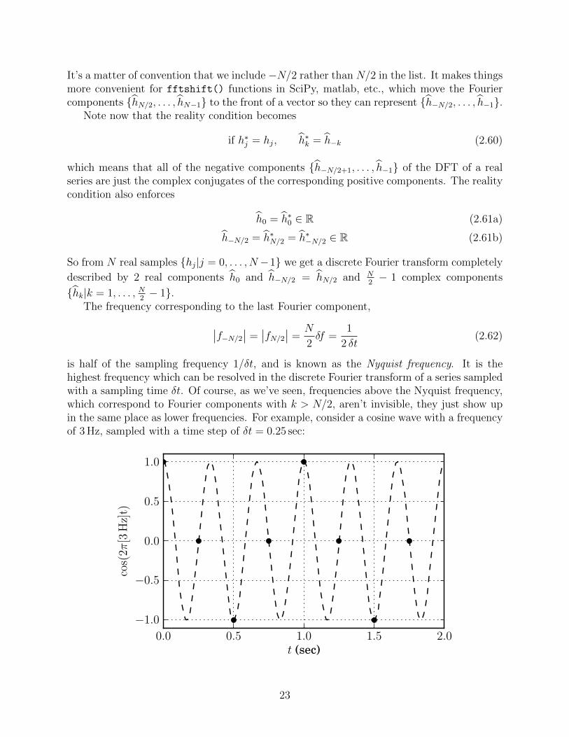
is half of the sampling frequency 1/δt, and is known as the Nyquist frequency. It is thehighest frequency which can be resolved in the discrete Fourier transform of a series sampledwith a sampling time δt. Of course, as we’ve seen, frequencies above the Nyquist frequency,which correspond to Fourier components with k > N/2, aren’t invisible, they just show upin the same place as lower frequencies. For example, consider a cosine wave with a frequencyof 3 Hz, sampled with a time step of δt = 0.25 sec:

23

If we just look at the dots, they don’t look like a 3 Hz cosine wave, but rather like one witha frequency of 1 Hz. And indeed, we’d get the exact same samples if we sampled a 1 Hz atthe same rate:

This is because f = 3 Hz is above the Nyquist frequency at this sampling rate, which isfNy = 2 Hz. The higher-frequency cosine wave has been aliased down to a frequency offNy − f = −1 Hz.

Note, in closing, that the range of independent frequencies, from −fNy to +fNy, is2 |fNy| = 1

δtso we can fill in the table for time-frequency resolution and extent:

Resolution Extentt discrete, δt duration Tf discrete, δf = 1

Tfinite, 2 |fNy| = 1

δt

Tuesday, September 21, 2010

3 Numerical Methods (guest lectures by Joshua Faber)

3.1 Orthogonal functions

As shown in previous classes, sets of orthogonal functions play an important role in thesolution of differential equations. A particularly useful choice is Chebyshev polynomials, asthey combine several of the benefits of Fourier methods with the simplicity of closed-formpolynomial expansions. Chebyshev polynomials have the distinction of being defined usingtrigonometric functions, which might seem at first glance like a contradiction in terms, withthe nth Chebyshev polynomial (beginning from n = 0) defined as

Tn(x) = cos(n arccosx) (3.1)

24

on the domain [−1, 1]. From the definition, it is clear that the range of the polynomialsis also [−1, 1], except for T0(x) = 1. Less clear is that these are polynomials at all. Todemonstrate this, we begin from the first two expressions T0(x) = 1 and T1(x) = x, and thennote that

2xTn(x)− Tn−1(x) = 2 cos(arccosx) cos(n arccosx)− cos([n− 1] arccosx)

= 2 cos(arccosx) cos(n arccosx)

− [cos(arccosx) cos(n arccosx) + sin(arccosx) sin(n arccosx)]

= cos(arccosx) cos(n arccosx)− sin(arccosx) sin(n arccosx)

= cos([n+ 1] arccosx) ≡ Tn+1(x)

(3.2)

and thus we can build up each new polynomial from the previous two using the recurrencerelation.

Chebyshev polynomials satisfy a weighted continuous orthogonality relation with weight(1− x2)−1/2 given by

∫ 1

−1

Tn(x)Tm(x)dx√

1− x2=

0 : n 6= m

π : n = m = 0

π/2 : n = m 6= 0

(3.3)

To prove this, we may use the trigonometric substitution x = cos θ → dx = − sin θdθ =−√

1− x2dθ, and note that

Tn(x) = Tn(cos θ) = cos(n arccos[cos θ]) = cos(nθ) (3.4)

finding that∫ 1

−1

Tn(x)Tm(x)dx√

1− x2=

∫ 0

π

cos(nθ) cos(mθ)(−dθ) =

∫ π

0

cos(nθ) cos(mθ)dθ (3.5)

The proof of orthogonality is actually a nice exercise∫ π

0

cos(nθ) cos(mθ)dθ =1

2

∫ π

0

[cos([m+ n]θ) + cos([m− n]θ)] dθ

=1

2(m+ n)sin([m+ n]θ)

∣∣π0

+1

2(m− n)sin([m− n]θ)

∣∣π0

(3.6)

If m 6= n, we get zero for both terms, if m = n 6= 0, the difference term yields π/2, and ifm = n = 0, each term yields π/2 for a total of π.

The Chebyshev polynomials are even and odd depending on the index, and their endpointvalues follow directly from the definition above. We find:

Tn(1) = 1 Tn(−1) = (−1)n (3.7a)

T ′n(1) = n T ′n(−1) = (−1)n+1n (3.7b)

25

From a practical standpoint, we often want to use a Chebyshev polynomial expansion toapproximate a function. Instead of performing a series of integrals over a set of complicatedfunctions, we can instead make use of the discrete orthogonality principle. Let

xk = cos

(π(k + 1/2)

n

); 0 ≤ k ≤ n− 1 (3.8)

be the n zeroes of Tn(x), known as the Gauss-Lobatto points in the language of orthogonalfunctions. The Chebyshev polynomials satisfy the discrete orthogonality relation

n−1∑k=0

Ti(xk)Tj(xk) =

0 : i 6= j

n : i = j = 0

n/2 : i = j 6= 0

(3.9)

which again may be derived from the properties of Fourier (cosine) modes.To approximate a function using Chebyshev polynomials, we can use the discrete orthog-

onality relation to our advantage. Assume that we have an expansion

f(x) ≈n−1∑j=0

cjTj(x) (3.10)

we find that

n−1∑k=0

f(xk)Tj(xk) =n−1∑k=0

ciTi(xk)Tj(xk) =

0 : i 6= j

nc0 : i = j = 0

nci/2 : i = j 6= 0

(3.11)

or inverting this result

c0 =1

n

n−1∑k=0

f(xk) (3.12a)

ci =2

n

n−1∑k=0

f(xk)Ti(xk) (3.12b)

3.1.1 Runge’s phenomenon and Minimax polynomials

Consider the curve f(x) = 11+25x2

, which looks like a slightly less-curved Gaussian, and issmooth (infinitely differentiable) everywhere. It is not, however a polynomial. If we were toapproximate it using a series of polynomials, our first attempt might be to try the Taylorseries at x = 0. Unfortunately, the radius of convergence is 1/5, so that doesn’t get us veryfar. . . Next, we might choose N + 1 evenly spaced points and try to fit a polynomial throughthem. You will find that this works very well for the center, but terribly at the edges. Infact, the errors near the edges grow in magnitude, without bound, as we increase the numberof points and the order of the polynomials with which we fit the function.

26

This is known as Runge’s Phenomenon, after the mathematician perhaps better known forco-developing a fourth-order differential equation evolution system. It turns out that bettersets of points for reducing the errors to zero is to choose them so that they are concentratednear the edges of the distribution. The optimal set of points would be to choose the points tobe zeros of a cosine function. Unfortunately, working out each of the polynomial coefficientsbased on these N points would typically very slow. If we fit using Chebyshev polynomials, onthe other hand, it is rather simple. As a result, Chebyshev interpolants fcheb(x) are knownto be the best simple approximant to the minimax polynomial of smooth functions f(x),where the minimax polynomial minimizes the quantity

max |f(x)− fcheb(x)| (3.13)

over the set of all nth order polynomials.

3.2 Differentiation and Chebyshev encounters of the second kind

One of the convenient things about expanding functions in terms of Chebyshev polynomials isthe fact we can solve differential equations, at least approximately, by converting continuoussystems to discrete linear algebra systems. To do so, we need to be able to take derivativesof Chebyshev polynomials. Using the trig definition, we find that

T ′n(x) =n sin(n arccosx)√

1− x2= n

sin(n arccosx)

sin(arccosx)≡ nUn−1(x) (3.14)

where we may define the functions Un(x), the so-called Chebyshev polynomials of the secondkind, through the relation

Un(x) ≡ sin([n+ 1] arccosx)

sin(arccosx)(3.15)

As with the Chebyshev polynomials of the first kind, it is not immediately obvious that theseare polynomials at all under the definition, though the differentiation identity above wouldseem to imply it. We note the following recurrence relation works as well. By inspection,U0(x) = 1 and U1 = 2 cos(arccosx) = 2x, and then we note that

Un(x) =sin([n+ 1] arccosx)

sin(arccosx)

=1

sin(arccosx)[sin(n arccosx) cos(arccosx) + cos(n arccosx) sin(arccosx)]

= xUn−1(x) + Tn(x)

(3.16)

It is important to note that unlike Chebyshev polynomials of the first kind, the second kindare not bounded between −1 and 1. Indeed, one can check that Un(1) = n and by symmetry,Un(−1) = (−1)nn. There are countless additional recurrence relations linking the two typesof Chebyshev polynomials, but we are most concerned here with this one:

Tn(x) = cos(n arccosx)sin(arccosx)

sin(arccosx)=

sin([n+ 1] arccosx)− sin([n− 1] arccos x)

2 sin(arccos x)=Un − Un−2

2(3.17)

27

This allows us to establish the following identity about derivatives, after rewriting the pre-vious equation as Un(x) = 2Tn(x) + Un−2(x):

d

dxTn(x) = nUn−1(x) = 2nTn−1(x) + nUn−3(x)

= 2nTn−1(x) + 2nTn−3(x) + nUn−5(x)

= 2nTn−1(x) + 2nTn−3(x) + 2nTn−5(x) + nUn−7(x)

(3.18)

and so on down the line until we reach either T1 or T0, terminating the sequence. It isworth noting that we can prove this relation using the complex exponential definition of trigfunctions as well. Define Θ = arccosx, and we find

Un(x) =sin([n+ 1]Θ)

sin Θ=

(ei(n+1)Θ − e−i(n+1)Θ)/2i

(eiΘ − e−iΘ)/2i

= einΘ + ei(n−2)Θ + e−(n−4)Θ + . . .+ e−i(n−2)Θ + e−inΘ

= 2[cos(nΘ) + cos([n− 2]Θ) + cos([n− 4]θ) + . . .]

= 2[Tn(x) + Tn−2(x) + Tn−4(x) + . . .]

(3.19)

Going back to the idea of a polynomial expansion, we see that if we have a function beingapproximated as a sum of polynomials,

f(x) ≈n∑i=0

ciTi(x) (3.20)

its derivative will involve a set of descending series:

df

dx= 2ncn(Tn−1 + Tn−3 + Tn−5 + . . .)

+2(n− 1)cn−1(Tn−2 + Tn−4 + . . .)

+2(n− 2)cn−2(Tn−3 + Tn−5 + . . .)

+ . . . =n−1∑i=0

diTi(x)

(3.21)

Looking carefully, we see that the only difference between the coefficient of the term Tn−1

and Tn−3 is generated by the coefficient cn−2, so that in general, if

di = di+2 + 2(i+ 1)ci+1 (3.22)

This result can also be derived using Clenshaw’s algorithm, which describes how to evaluatecombinations of polynomials defined by a recurrence relation. Similarly, for integration, wecan essentially read the identity above backwards, finding that if

∫f(x)dx ≈

∑biTi(x), then

bi =ci−1 − ci+1

2i(3.23)

28

3.3 Gauss’s phenomenon

Chebyshev interpolation is spectrally accurate for smooth (infinitely differentiable) functions:if we approximate a given function on [−1, 1] using n polynomial coefficients, any errorestimate you like including the Li, L2 and L∞ error will scale like kn, or in other words,exponentially. If the function we wish to interpolate is not smooth, this is no longer true.The error instead will decrease like nd+2, where the function can be differentiated d times.Luckily, there is a simple solution to deal with these case. Consider a function we wish tointerpolate that is smooth on the interval [a, b]. If we define a rescaled variable X through therelation x = (a+ b)/2 + (a− b)X/2, so that the smooth interval satisfies −1 < X < x, thenTn(X) will satisfy the exponential convergence property. If the function to be interpolated ispiecewise smooth, we may interpolate each segment using a different set of scaled Chebyshevpolynomials, to yield the required accuracy.

Thursday, September 23, 2010

3.4 Elliptic and Hyperbolic equations: an overview

Consider a second order differential equation in a k-dimensional space:

k∑m=0

k∑n=0

Amn∂

∂xm

(∂f

∂xn

)+

k∑p=0

Bp∂f

∂xp= F (f) (3.24)

If the matrix A is positive definite everywhere, we call the equation “elliptic”.Positive definite implies all eigenvalues of the matrix are positive. Rather than focus

on the matrix aspects, we can concentrate on the physical examples. The most famouselliptic equation is the Poisson equation, which describes, among other things, Newtoniangravitational and electric fields:

∇2Φ =

(∂2

∂x2+

∂2

∂y2+

∂2

∂z2

)Φ = 4πGρ (3.25)

You’ve already seen that the left hand side takes different forms in different coordinatesystems, but all are elliptic.

Hyperbolic equations look much the same if the sign of one of the terms is negative, aswe find in the wave equation:

∂2f

∂t2− v2∂

2f

∂x2= 0 (3.26)

From the standpoint of working with the equations, they could hardly be more different.Hyperbolic equations evolve forward in time (or whatever you name the variable with theopposite signature in the second derivative), and require the specification of initial data(values of the function f and its first derivative), and possibly boundary conditions dependingon the particular equation, solution, domain, and numerical scheme. These are generallyreferred to as “Initial Value Problems”. On the boundary of our domain, we need to imposesome form of boundary condition, which typically comes in one of three types:

1. Dirichlet: f(x) is a specified function on the boundary

29

2. Von Neumann: ∇Nf(x) is specified on the boundary, where the gradient is takennormal to the boundary

3. Robin: H[f(x),∇Nf(x)], some function of the value of the function and its normalgradient, is specified on the boundary

The boundary can be any surface, including one located at spatial infinity.

3.5 The Poisson equation

It is not difficult to find ways to solve the Poisson equation, which arises for both gravitationalfields and electric fields in Newtonian physics. In some ways, the problem is choosing amethod.

We can use:

1. Convolution

2. multipole moments (for the exterior)

3. Spectral methods

We will discuss the first two in turn.

3.5.1 Convolution

Mathematically speaking, convolution is the most elegant approach to the solution of thePoisson equation. We begin with a known integral form of the solution to the Poissonequation:

[∇2Φ](~r) = 4πGρ(~r)⇒ Φ(~r) =y Gρ(~r ′)

|~r − ~r ′|d3V ′ (3.27)

The key thing to notice is that we have one term involving a function of the variable weare integrating over (~r ′), and one that depends on a difference between a fixed point in theintegral (~r) and the integration variable (~r ′). In general, there is a simple way to solve theseproblems using Fourier transforms, where we will make use of the fact that Fourier forwardand reverse transforms are inverse operations.

Denoting the forward Fourier transform Fg(x) =∫∞−∞ e

2πikxg(x)dx, and consideringthe case of one-dimensional integrals, we find that

FΦ(x) = G

∫ ∞−∞

dx e2πikx

∫ ∞−∞

dx′ ρ(x′) |x− x′|−1(3.28)

Letting y = x− x′, we find x = x′ + y, and dx dx′ = dx′ dy and the integral becomes

FΦ(x) = G

∫ ∞−∞

∫ ∞−∞

dy dx′e2πik(x′+y)ρ(x′) |y|−1

= G

(∫ ∞−∞

dx′ e2πikx′ρ(x′)

)(∫ ∞−∞

dy e2πiky |y|−1

)= Fρ(x) · F|x|−1

(3.29a)

Φ(x) = F−1Fρ(x) · F|x|−1

(3.29b)

30

There is nothing special about the functions we convolve to find the potential, and thismethod, to Fourier transform both functions, multiply the transforms together pointwise,and then inverse transform, is the general technique for performing any convolution integral.

3.5.2 Mode expansion of the Poisson equation

By using spherical harmonics, we can break down the Poisson equation, which is linear, intoindependent multipole components. By defining

ρ`m(r) ≡x

ρ(r, θ, φ)Y ∗`m(θ, φ)d2Ω (3.30)

and noting thatsY`′m′Y

∗`md

2Ω = δ``′δmm′ we may split the source term into a set of orthog-onal moments, such that

ρ(r, θ, φ) =∑`,m

ρ`m(r)Y`m(θ, φ) (3.31)

Each term ρ`m generates a term in the solution Φ`m.There is one issue with solving the general Poisson equation. For each mode, we need to

solve the second order equation

1

r2

∂

∂r

(r2∂R`m(r)

∂r

)− `(`+ 1)

r2R`m(r) = 4πGρ`m(r) (3.32)

Which, being linear, will have a particular solution Rp;`m(r) and two homogeneous solutions.For spherical harmonics, these are easily found to be

R`m(r) = Rp;`m(r) + Cr` +Dr−(`+1) (3.33)

but we have difficulty if we want the solution to remain finite at either r = 0 or r → ∞.In practice, if we have a compact matter distribution, we use the trick to split the domaininto two, radially. In the innermost domain, we set D = 0 so that the solution doesn’t blowup at the origin, whereas in the outer one, we set C = 0 to avoid divergence at spatialinfinity. We have two undetermined coefficients, but these may be fixed by requiring thatR(r) is continuous and differentiable at the interface, as would be expected for a second-order differential equation. Note that this implies that if a matter distribution has a sphericalharmonic term ρ`m, the resulting field falls off like r−`−1.

3.5.3 The Iron sphere theorem

The easiest mode to calculate of the mass distribution is the Y00 mode, which is given bythe integral

ρ00 =y

ρ(~r) d3V = M (3.34)

yielding a potential Φ00 = −GM/r. In practical terms, this implies the Iron Sphere Theorem:From the outside, one can tell the mass of a spherically symmetric mass distribution, butnot its internal structure. From the inside of a spherical shell, there is no force at all. Theproof, which reflects a 2-d integral over angles, says that since the area of a patch on opposite

31

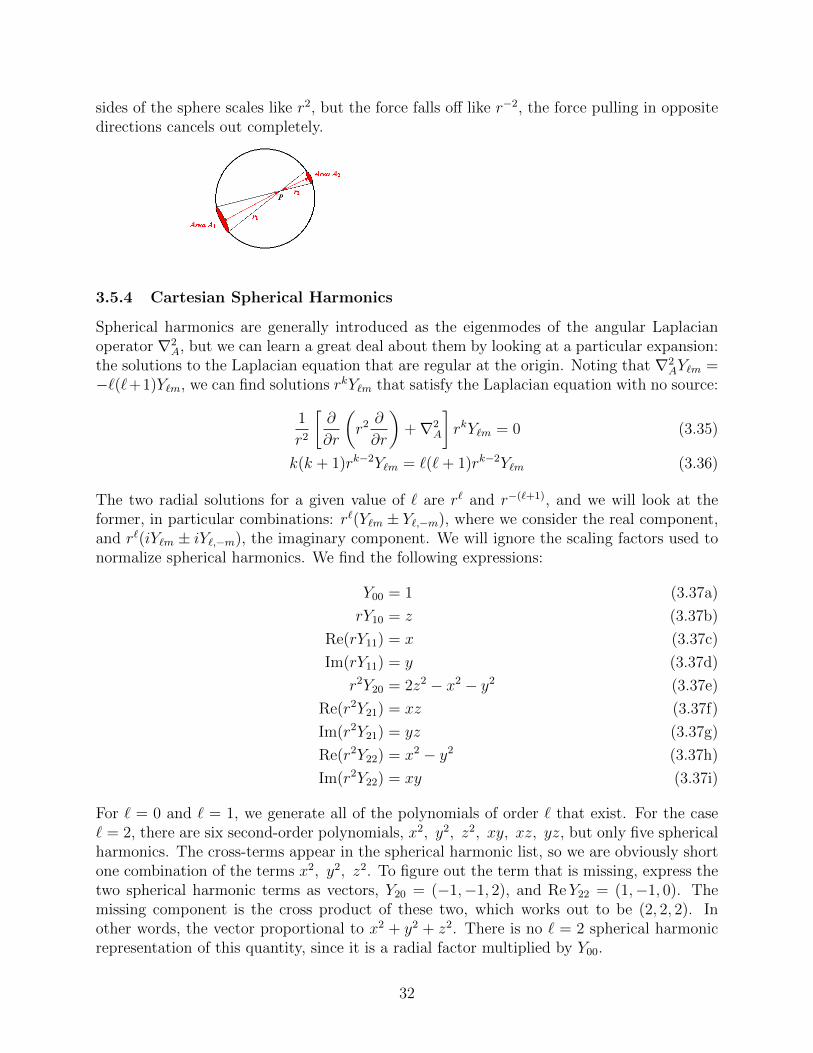
sides of the sphere scales like r2, but the force falls off like r−2, the force pulling in oppositedirections cancels out completely.

3.5.4 Cartesian Spherical Harmonics

Spherical harmonics are generally introduced as the eigenmodes of the angular Laplacianoperator ∇2

A, but we can learn a great deal about them by looking at a particular expansion:the solutions to the Laplacian equation that are regular at the origin. Noting that ∇2

AY`m =−`(`+1)Y`m, we can find solutions rkY`m that satisfy the Laplacian equation with no source:

1

r2

[∂

∂r

(r2 ∂

∂r

)+∇2

A

]rkY`m = 0 (3.35)

k(k + 1)rk−2Y`m = `(`+ 1)rk−2Y`m (3.36)

The two radial solutions for a given value of ` are r` and r−(`+1), and we will look at theformer, in particular combinations: r`(Y`m ± Y`,−m), where we consider the real component,and r`(iY`m ± iY`,−m), the imaginary component. We will ignore the scaling factors used tonormalize spherical harmonics. We find the following expressions:

Y00 = 1 (3.37a)

rY10 = z (3.37b)

Re(rY11) = x (3.37c)

Im(rY11) = y (3.37d)

r2Y20 = 2z2 − x2 − y2 (3.37e)

Re(r2Y21) = xz (3.37f)

Im(r2Y21) = yz (3.37g)

Re(r2Y22) = x2 − y2 (3.37h)

Im(r2Y22) = xy (3.37i)

For ` = 0 and ` = 1, we generate all of the polynomials of order ` that exist. For the case` = 2, there are six second-order polynomials, x2, y2, z2, xy, xz, yz, but only five sphericalharmonics. The cross-terms appear in the spherical harmonic list, so we are obviously shortone combination of the terms x2, y2, z2. To figure out the term that is missing, express thetwo spherical harmonic terms as vectors, Y20 = (−1,−1, 2), and ReY22 = (1,−1, 0). Themissing component is the cross product of these two, which works out to be (2, 2, 2). Inother words, the vector proportional to x2 + y2 + z2. There is no ` = 2 spherical harmonicrepresentation of this quantity, since it is a radial factor multiplied by Y00.

32

3.5.5 Multipole moments

If we have a compact density, i.e., one which is non-zero over a finite domain, we can performa multipole expansion of the solution. This involves breaking the source term into sphericalharmonic modes, and solving each in turn. We have to remember that since the potentialgoes to a constant as r →∞, our vacuum solution involves the terms in the form r−(`+1)Y`m.The general solution may be written

Φ = G

[M

r+∑i

pixi

r2+

1

2

∑i,j

Qijxixj

r3+ . . .

](3.38)

where xi is the unit normal vector at a given point located at radius r. The monopolemoment of the density distribution is given by the mass, M =

tρd3V , the dipole term

collects the ` = 1 Y`m terms:

pi ≡y

ρxid3V (3.39)

and the Qij terms are the traceless quadrupole moments:

Qij ≡y (

xixj − 1

3δijr2

)ρ(~r) d3V (3.40)

Why traceless? Based on previous discussion, the ` = 2 spherical harmonics don’t contain aterm that represents a pure radial component r2, and thus such modes don’t affect the grav-itational potential outside of the matter distribution. This is commonly known as Newton’siron sphere theorem: a hollow sphere from the outside has the same gravitational potentialas a solid one of the same mass. There are, of course, higher order moments as well, but theforms of each term get significantly more complicated as we progress.

Tuesday, September 28, 2010

4 Spectral Analysis of Random Data

4.1 Amplitude Spectrum

Given a real time series h(t) we know how to construct its Fourier transform

h(f) =

∫ ∞−∞

h(t) e−i2πft dt (4.1)

or the equivalent discrete Fourier transform from a set of samples hj|j = 0, . . . , N − 1:

hk =N−1∑j=0

hj e−i2πjk/N (4.2)

where hk δt ∼ h(fk).

33

Think about the physical meaning of h(f), by breaking this complex number up into anamplitude and phase

h(f) = A(f) eiφ(f) . (4.3)

If h(t) is real, the condition h(−f) = h∗(f) = A(f)e−iφ(f) means A(−f) = A(f) andφ(−f) = −φ(f). Thus we can write the inverse Fourier transform as

h(t) =

∫ 0

−∞A(f) ei[2πft+φ(f)] df +

∫ ∞0

A(f) ei[2πft+φ(f)] df

=

∫ ∞0

A(f)(ei[2πft+φ(f)] + e−i[2πft+φ(f)]

)df

=

∫ ∞0

2A(f) cos (2πft+ φ(f))

(4.4)

So A(f) is a measure of the amplitude at frequency f and φ(f) is the phase.Note also that ∫ ∞

−∞[h(t)]2 dt =

∫ ∞−∞

∣∣∣h(f)∣∣∣2 df (4.5)

This works pretty well if the properties of h(t) are deterministic. But suppose h(t) ismodelled as random, i.e., it depends on a lot of factors we don’t know about, and all wecan really do is make statistical statements. What is a sensible description of the spectralcontent of h?

4.2 Random Variables

Consider a random variable x. Its value is not known, but we can talk about statisticalexpectations as to its value. We will have a lot more to say about this soon, but for nowimagine we have a lot of chances to measure x in an ensemble of identically-prepared systems.The hypothetical average of all of those imagined measurements is called the expectation valueand we write it as 〈x〉. (Another notation is E[x].) We can also take some known function fand talk about the expectation value 〈f(x)〉 corresponding to a large number of hypotheticalmeasurements of f(x).

The expectation value of x itself is the mean, sometimes abbreviated as µ. (This nameis taken by analogy to the mean of an actual finite ensemble.) Since x is random, though,x won’t always have the value 〈x〉. We can talk about how far off x typically is from itsaverage value 〈x〉. Note however that

〈x− µ〉 = 〈x〉 − 〈µ〉 = 〈x〉 − µ = 0 (4.6)

since the expectation value is a linear operation (being the analogue of an average), and theexpectation value of a non-random quantity is just the quantity itself. So instead of themean deviation from the mean, we need to consider the mean square deviation from themean ⟨

(x− 〈x〉)2⟩

(4.7)

This is called the variance, and is sometimes written σ2. Its square root, the root meansquare (RMS) deviation from the mean, is the standard deviation.

34

4.2.1 Random Sequences

Now imagine we have a bunch of random variables xj; in principle each can have its ownmean µj = 〈xj〉 and variance σ2

j = 〈(xj − µj)2〉. But we can also think about possiblecorrelations σ2

j` = 〈(xj − µj)(x` − µ`)〉; if the variables are uncorrelated σ2j` = δj` σ

2j , but

that need not be the case.Think specifically about a series of N samples which are all uncorrelated random variables

with zero mean and the same variance:

〈xj〉 = 0; 〈xjx`〉 = δj` σ2 ; (4.8)

what are the characteristics of the discrete Fourier transform of this sequence?

xk =N−1∑j=0

xj e−i2πjk/N (4.9)

Well,

〈xk〉 =N−1∑j=0>

0〈xj〉 e−i2πjk/N = 0 (4.10)

and

〈xkx∗`〉 =N−1∑j=0

N−1∑n=0

〈xjxn〉 e−i2π(jk−n`)/N =N−1∑j=0

σ2e−i2πj(k−`)/N = Nσ2δk,` mod N (4.11)

so the Fourier components are also uncorrelated random variables with variance⟨|xk|2

⟩= Nσ2 (4.12)

Note this is independent of k, which is maybe a bit surprising. After all, it’s natural to thinkall times are alike, but all frequencies need not be. Random data like this, which is the sameat all frequencies, is called “white noise”. To gain some more insight into white and colorednoise, it helps to think about the same thing in the idealization of the continuous Fouriertransform.

4.3 Continuous Random Data

Think about the continuous-time analog to the random sequence considered in section 4.2.1.This is a time series x(t) which is characterized by statistical expectations. In particular wecould talk about its expectation value

〈x(t)〉 = µ(t) (4.13)

and the expectation value of the product of samples taken at possibly different times

〈x(t)x(t′)〉 = Kx(t, t′) (4.14)

(it’s conventional not to subtract out µ(t) here). Note that 〈x(t)〉 is not the time-averageof a particular instantiation of x(t), although the latter may sometimes be used to estimatethe former.

35

4.3.1 White Noise

Now, for white noise we need the continuous-time equivalent of (4.8), in which the data isuncorrelated with itself except at the very same time. In the case of continuous time, thesensible thing is the Dirac delta function, so white noise is characterized by

〈x(t)x(t′)〉 = K0 δ(t− t′) (4.15)

where K0 is a measure of how “loud” the noise is. In the frequency domain, this means

〈x(f)x∗(f ′)〉 =

∫ ∞−∞

∫ ∞−∞〈x(t)x(t′)〉 e−i2π(ft−f ′t′) dt dt′ = K0

∫ ∞−∞

e−i2π(f−f ′)t dt

= K0 δ(f − f ′) .(4.16)

4.3.2 Colored Noise

A lot of times, the quantity measured in an experiment is related to some starting quantityby a linear convolution, so even if we start out with white noise, we could end up dealingwith something that has different properties. If we consider some random variable h(t) whichis produced by convolving white noise with a deterministic response function R(t − t′), sothat

h(t) =

∫ ∞−∞

R(t− t′)x(t′) dt′ (4.17)

and in the frequency domainh(f) = R(f)x(f) (4.18)

we have ⟨h(f)h∗(f ′)

⟩= K0

∣∣∣R(f)∣∣∣2 δ(f − f ′) . (4.19)

Note that even in this case,⟨|h(f)|2

⟩blows up, so simply looking at the magnitudes of

Fourier components is not the most useful thing to do. However, the quantity K0

∣∣∣R(f)∣∣∣2

which multiplies the delta function can be well-behaved, and gives a useful spectrum. We’llsee that this is the power spectral density Sh(f), which we’ll define more carefully in a bit.

We can also go back into the time domain in this example, and calculate the autocorre-lation

Kh(t, t′) = 〈h(t)h(t′)〉 =

∫ ∞−∞

∫ ∞−∞

R(t− t1)R(t′ − t′1) 〈x(t1)x(t′1)〉 dt1 dt′1

=

∫ ∞−∞

K0R(t− t1)R(t′ − t1) dt1

(4.20)

which is basically the convolution of the response function with itself, time reversed; unlikein the case of white noise, where Kx(t, t

′) was a delta function, this will in general be finite.Note that in this example, the autocorrelation Kh(t, t

′) is unchanged by shifting both ofits arguments:

Kh(t+ τ, t′ + τ) = K0

∫ ∞−∞

R(t− [t1 − τ ])R(t′ − [t1 − τ ]) dt1

= K0

∫ ∞−∞

R(t− t2)R(t′ − t2) dt2 = Kh(t, t′)

(4.21)

36

where we make the change of integration variables from t1 to t2 = t1 − τ . This means thatin this colored noise case the autocorrelation is a function only of t− t′.

Thursday, September 30, 2010

4.4 Wide-Sense Stationary Data

We now turn to a general formalism which incorporates our observations about colored noise.A random time series h(t) is called wide-sense stationary if it obeys

〈h(t)〉 = µ = constant (4.22)

and〈h(t)h(t′)〉 = Kh(t− t′) . (4.23)

Clearly, both our white noise and colored noise examples were wide-sense stationary. Theappearance of a convolution in the time-domain (4.20) a product in the frequency domain(4.19) suggests to us that the Fourier transform of the auto-correlation function Kh(t − t′)is a useful quantity. We this define the power spectral density as

Sh(f) =

∫ ∞−∞

Kh(τ) e−i2πfτ dτ . (4.24)

Note that by the construction (4.23) the autocorrelation is even in its argument [Kh(τ) =Kh(−τ)] so the PSD of real data will be real and even in f .

We can then show that for a general wide-sense stationary process,⟨h(f)h∗(f ′)

⟩=

∫ ∞−∞

∫ ∞−∞〈h(t)h(t′)〉 e−i2π(ft−f ′t′) dt dt′

=

∫ ∞−∞

∫ ∞−∞

Kh(τ) e−i2πfτe−i2π(f−f ′)t′ dτ dt′ = δ(f − f ′)Sh(f) ,

(4.25)

where we make the change of variables from t to τ = t− t′.

4.4.1 Symmetry Properties of the Auto-Correlation and the PSD

We can see from the definition (4.23) and the result (4.25) that, for real data, both Kh(τ)and Sh(f) are real and even, and in particular that Sh(f) = Sh(−f). (Of course the factthat Kh(τ) and Sh(f) are Fourier transforms of each other means that once we know thesymmetry properties of one, we can deduce the symmetry properties of the other.) Becauseit’s defined at both positive and negative frequencies, the power spectral density Sh(f) thatwe’ve been using is called the two-sided PSD. Since the distinction between positive andnegative frequencies depends on things like the sign convention for the Fourier transform,it is sometimes considered more natural to define a one-sided PSD which is defined only atnon-negative frequencies, and contains all of the power at the corresponding positive andnegative frequencies:

S1-sidedh (f) =

Sh(0) f = 0

Sh(−f) + Sh(f) f > 0(4.26)

37

Apparently, for real data, S1-sidedh (f) = 2Sh(f) when f > 0.

If the original time series is not actually real, there is a straightforward generalization ofthe definition of the auto-correlation function:

〈h(t)h∗(t′)〉 = Kh(t− t′) (4.27)

The PSD is then defined as the Fourier transform of this, and (4.25) holds as before. Exam-ination of (4.27) and (4.25) shows that, for complex data, the symmetry properties whichremain are

• Kh(−τ) = K∗h(τ)

• Sh(f) is real.

4.5 Power Spectrum Estimation

Suppose we have a stretch of data, duration T , sampled at intervals of δt, from a wide-sensestationary data stream,

hj = h(t0 + j δt) (4.28)

where the autocorrelationKh(t− t′) = 〈h(t)h(t′)〉 (4.29)

and its Fourier transform the PSD

Sh(f) =

∫ ∞−∞

Kh(τ) e−i2πfτ dτ (4.30)

are unknown. How do we estimate Sh(f)? One idea, keeping in mind that⟨h(f)h∗(f ′)

⟩= δ(f − f ′)Sh(f) , (4.31)

is to use the discrete Fourier components to construct∣∣∣hk∣∣∣2 (4.32)

this is, up to normalization, the periodogram. Now, we’re going to have to be a little carefulabout just using the identification

hk δt ∼ h(fk) (4.33)

where

fk = k δf =k

T; (4.34)

after all, taking that literally would mean setting f and f ′ both to fk and evaluating the deltafunction at zero argument. So we need to be a little more careful about the approximationthat relates the discrete and continuous Fourier transforms.

38

4.5.1 The Discretization Kernel ∆N(x)

If we substitute the continuous inverse Fourier transform into the discrete forward Fouriertransform, we find

hk =N−1∑j=0

h(t0 + j δt) e−i2πjk/N =N−1∑j=0

∫ ∞−∞

h(f) e−i2πjk/N ei2πf j δt df

=

∫ ∞−∞

(N−1∑j=0

e−i2πj(fk−f)δt

)h(f) df =

∫ ∞−∞

∆N([fk − f ]δt) h(f) df

(4.35)

where we have defined8

∆N(x) =N−1∑j=0

e−i2πjx . (4.36)

Let’s look at some of the properties of this ∆N(x). First, if x is an integer,

∆N(x) =N−1∑j=0

e−i2πjx =N−1∑j=0

1 = N (x ∈ Z) (4.37)

Next, note that ∆N(x) is periodic in x with period 1, since

∆N(x+ 1) =N−1∑j=0

e−i2πj(x+1) =N−1∑j=0

e−i2πjxe−i2πj =N−1∑j=0

e−i2πjx = ∆N(x) . (4.38)

Note that this is not surprising for something that relates a discrete to a continuous Fouriertransform; incrementing [fk − f ]δt by 1 is the same as decrementing f by 1/δt, which istwice the Nyquist frequency. This is just the usual phenomenon of aliasing, where manycontinuous frequency components, separated at intervals of 1/δt, are mapped onto the samediscrete component.

Note also that

∆N(`/N) =N−1∑j=0

e−i2πj`/N = 0 ` ∈ Z and ` 6= 0 mod N (4.39)

of course, it’s sort of cheating to quote that result from before, since we got it by actuallyevaluating the sum, so let’s do that again. Since

(1− aN) = (1− a)N−1∑j=0

aj , (4.40)

if we set a = e−i2πx, we get, for x /∈ Z (which means a 6= 1),

∆N(x) =1− e−i2πNx

1− e−i2πx=e−iπNx

e−iπxeiπNx − e−iπNx

ei2πx − e−i2πx= e−iπ(N−1)x sinπNx

sin πx(4.41)

8This is closely related to the Dirichlet kerneln∑

k=−n

e−ikx = sin([2n+ 1]x2

)/ sin

(x2

).

39

so, to summarize,

∆N(x) =

N , x ∈ Ze−iπ(N−1)x

(sinπNxsinπx

), x /∈ Z

(4.42)

4.5.2 Derivation of the Periodogram

Now that we have a more precise relationship between hk and h(f), we can think about∣∣∣hk∣∣∣2, and in particular its expectation value:⟨∣∣∣hk∣∣∣2⟩ =

∫ ∞−∞

∫ ∞−∞

∆N([fk − f ]δt)∆∗N([fk − f ′]δt)⟨h(f)h∗(f ′)

⟩df df ′

=

∫ ∞−∞|∆N([fk − f ]δt)|2 Sh(f) df

(4.43)

Let’s get a handle on

|∆N(x)|2 =

(sin πNx

sin πx

)2

(4.44)

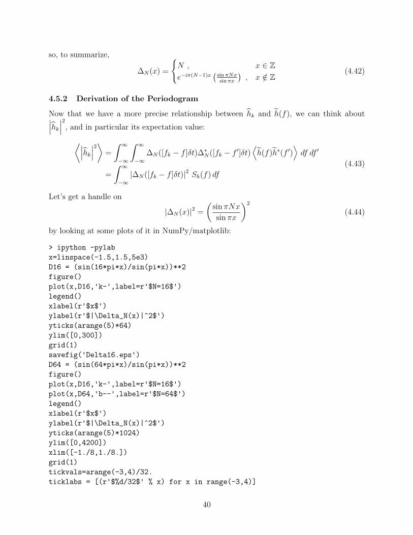
by looking at some plots of it in NumPy/matplotlib:

> ipython -pylab

x=linspace(-1.5,1.5,5e3)

D16 = (sin(16*pi*x)/sin(pi*x))**2

figure()

plot(x,D16,'k-',label=r'$N=16$')

legend()

xlabel(r'$x$')

ylabel(r'$|\Delta_N(x)|^2$')

yticks(arange(5)*64)

ylim([0,300])

grid(1)

savefig('Delta16.eps')

D64 = (sin(64*pi*x)/sin(pi*x))**2

figure()

plot(x,D16,'k-',label=r'$N=16$')

plot(x,D64,'b--',label=r'$N=64$')

legend()

xlabel(r'$x$')

ylabel(r'$|\Delta_N(x)|^2$')

yticks(arange(5)*1024)

ylim([0,4200])

xlim([-1./8,1./8.])

grid(1)

tickvals=arange(-3,4)/32.

ticklabs = [(r'$%d/32$' % x) for x in range(-3,4)]

40

xticks(tickvals,ticklabs)

savefig('Delta64.eps')

If we look for N = 16, we see that |∆N(x)|2 is indeed periodic, with period 1, and has thevalue N2 = 162 = 256 for integer x:

1.5 1.0 0.5 0.0 0.5 1.0 1.5x

0

64

128

192

256

|

N(x)|2

N=16

It’s also pretty sharply peaked at integer values; we can zoom in and compare it to |∆N(x)|2for N = 64:

41

3/32 2/32 1/32 0/32 1/32 2/32 3/32x

0

1024

2048

3072

4096

|

N(x)|2

N=16

N=64

We see now that the peak at x = 0 is at N2 = 642 = 4096. Note we can also see the zerosat non-zero integer multiples of 1/N for both functions. And the function is getting moresharply peaked as N gets larger.

We can see, then, that |∆N(x)|2 is acting as an approximation to a sum of Dirac deltafunctions (one peaked at each integer value of x), and this approximation is better for higherN . We can write this situation as

|∆N(x)|2 ≈ NN∞∑

s=−∞

δ(x+ s) (4.45)

To get the overall normalization constant NN , we have to integrate both sides of (4.45),using the fact that ∫ ∞

−∞δ(x) dx = 1 (4.46)

Of course, we don’t actually want to integrate |∆N(x)|2 from −∞ to∞, because it’s periodic,and we’re bound to get something infinite when we add up the contributions from the infinitenumber of peaks. And likewise, the right-hand side contains an infinite number of deltafunctions. So we should just integrate over one cycle, using∫ 1/2

−1/2

δ(x) dx = 1 (4.47)

and choose NN so that∫ 1/2

−1/2

|∆N(x)|2 dx = NN∞∑

s=−∞

∫ 1/2

−1/2

δ(x+ s) dx = NN (4.48)

42

We could explicitly evaluate (or look up) the integral of |∆N(x)|2 =(

sinπNxsinπx

)2, but it turns

out to be easier to evaluate it as

NN =

∫ 1/2

−1/2

∆N(x)[∆N(x)]∗ dx =

∫ 1/2

−1/2

N−1∑j=0

e−i2πjxN−1∑`=0

ei2π`x dx =N−1∑j=0

N−1∑`=0

∫ 1/2

−1/2

e−i2π(j−`)x dx .

(4.49)But the integral is straighforward:∫ 1/2

−1/2

e−i2π(j−`)x dx =

1 j = `sin(π[j−`])π(j−`) j 6= `

= δj` (4.50)

so ∫ 1/2

−1/2

e−i2π(j−`)x dx = δj` j, ` ∈ Z (4.51)

and the normalization constant is

NN =N−1∑j=0

N−1∑`=0

δj` = N (4.52)

and

|∆N(x)|2 ≈ N∞∑

s=−∞

δ(x− s) (4.53)

We can now substitute this back into (4.43) and find⟨∣∣∣hk∣∣∣2⟩ =

∫ ∞−∞|∆N([fk − f ]δt)|2 Sh(f) df ≈ N

∞∑s=−∞

∫ ∞−∞

δ([fk − f ]δt− s)Sh(f) df

=N

δt

∞∑s=−∞

∫ ∞−∞

δ(f − [fk − s/δt])Sh(f) df =N

δt

∞∑s=−∞

Sh(fk − s/δt) .(4.54)

That means that the correct definition of the periodogram is

Pk :=δt

N

∣∣∣hk∣∣∣2 . (4.55)

Its expectation value is

〈Pk〉 =

∫ ∞−∞

δt

N|∆N([fk − f ]δt)|2 Sh(f) df ≈

∞∑s=−∞

Sh(fk − s/δt) (4.56)

4.5.3 Shortcomings of the Periodogram

There are a few ways in which the periodogram is not quite an ideal estimate of the underlyingPSD Sh(f):

43

1. As noted above, it’s not actually an approximation to the PSD at fk, but to that,plus the PSD at fk + 1/δt plus the PSD at fk + 2/δt etc. This is the usual aliasingphenomenon; since 1/δt is twice the Nyquist frequency, we can avoid it by doing somesort of analog processing of our original time series so that Sh(f) = 0 if |f | is abovethe Nyquist frequency, and then confining attention to k between −N/2 and N/2− 1so that fk is between minus Nyquist and Nyquist. We’ll assume we’ve done that.

2. The function |∆N([fk − f ]δt)|2 is not actually the greatest approximation to the Diracdelta function, because of the “ringing” in the side lobes outside of the main peak. Thismeans the periodogram estimate at a given frequency will be “contaminated” with datafrom nearby frequencies to a greater degree than necessary. This phenomenon is calledspectral leakage. The source of this problem is that by sampling h(t) only from t0 tot0 + T , we’ve effectively multiplied it by a rectangular window in the time domain

Wr(t) =

0 t < t0

1 t0 ≤ t < T

0 t ≥ T

(4.57)

which means the Fourier transform is the convolution of W (f) with h(f). We knowthat the Fourier transform of a rectangle is not the nicest thing in the world, so we’rebetter off multiplying the data by a window which more smoothly rises from 0 to 1and then goes back down again, since its Fourier transform will stretch out less infrequencies. We won’t elaborate on that further right now, but see, e.g., Section 13.4of Numerical Recipes for more.

3. While Pk has the right expected mean (4.56), its expected variance⟨(Pk − 〈Pk〉)2

⟩=⟨P 2k

⟩− 〈Pk〉2 , (4.58)

which is a measure of the square of the typical error associated with the estimate, islarger than we’d like. We can look at

⟨P 2k

⟩=

(δt

N

)2 ⟨hkh

∗khkh

∗k

⟩; (4.59)

now, we can’t actually evaluate this without saying more about the properties of h(t)than we’ve specified. We’ve talked about the expectation value and the autocorrelation,but not the full distribution of probabilities of possible values. We’ll soon develop themachinery to consider such things, but for now, we’ll just state that for some choicesof that underlying distribution⟨

hkh∗khkh

∗k

⟩∼ 2

⟨hkh

∗k

⟩⟨hkh

∗k

⟩(4.60)

and if that’s the case ⟨P 2k

⟩∼ 2

(δt

N

∣∣∣hk∣∣∣)2

= 2 〈Pk〉2 (4.61)

44

but that means the expected mean square error is the square of the expectation valueitself: ⟨

(Pk − 〈Pk〉)2⟩∼ 〈Pk〉2 ≈ [Sh(fk)]

2 (4.62)

so we have an estimate of the power whose typical error is the same size as the estimateitself!

Note that this is independent of T , which means you don’t get any better of an es-timate of the PSD of a wide-sense stationary process by including more data in theperiodogram. This is perhaps not so surprising if we recall that the discrete Fouriertransform was developed in the context of deterministic data. Having a longer stretchof data produces higher resolution in the frequency domain, because δf = 1

T. So

that means if you construct a periodogram from 50 seconds of data, you get not-very-accurate PSD estimates at frequencies separated by 0.02 Hz. If you use 200 seconds,you get PSD estimates at more frequencies, just 0.005 Hz apart, but they’re not anymore accurate; they still have RMS expected errors equal to their expectation values.However, if the underlying PSD Sh(f) doesn’t vary much as a function of frequency,then Sh(43.000 Hz), Sh(43.005 Hz), Sh(43.010 Hz) etc may be more or less the same,and so the corresponding periodograms will be estimates of roughly the same quantity.So you’d want to average those together to get a more accurate estimate. I.e., youwant to lower the frequency resolution.

You can get a lower frequency resolution by doing your Fourier transforms over ashorter time, i.e., by breaking up the time T into Nc chunks, each of duration T/Nc,then doing discrete Fourier transforms over the N = T

Ncδt samples in each chunk. Theperiodogram from the αth chunk is then

Pαk =δt

N

∣∣∣hk∣∣∣2 ; (4.63)

its frequency resolution is

δf =1

N δt=NcT

. (4.64)

Each periodogram has expected mean

〈Pαk〉 ≈ P (fk) = P (kδf) (4.65)

and variance ⟨P 2αk

⟩− 〈Pαk〉 ≈ [P (fk)]

2 (4.66)

as before. But we can take the average of all Nc periodograms

P k =1

Nc

Nc−1∑α=0

Pαk (4.67)

and since averaging independent random variables lowers the resulting variance,⟨P k

⟩= P (fn) (4.68)

45

and variance ⟨P

2

k

⟩−⟨P k

⟩≈ [P (fk)]

2

Nc. (4.69)

So the error in the PSD estimation shrinks like 1/√Nc. We can get a more accurate

estimate of the PSD by breaking the time up into chunks and averaging, but at theexpense of a coarser frequency resolution. The appropriate tradeoff depends on thesharpness of the features that we want to resolve in the spectrum.

46