Notes on Complex Fluids: Kinetic Theory - UC Santa...

Notes on Complex Fluids: Kinetic Theory

Hector D. Cenicerosc© Draft date January 4, 2011

Chapter 1

Introduction

1.1 What are Complex Fluids?

Complex fluids include polymeric liquids, colloidal suspensions (gels, sols, and emul-sions), liquid crystalline materials, foams, powders, and granular materials. Thesenon-Newtonian fluids are ubiquitous: milk, ketchup, mustard, molten chocolate,ice cream, shampoo, toothpaste, blood, saliva, etc. For an illustrative introductionsee the book by Larson [5] From the technological point of view, complex fluidshave significant relevance as they are precursors of advanced materials. Many ofthese materials are processed in liquid form and as such they are complex fluids, forexample all plastics and resins and liquid crystalline polymers (LCPs).

Complex fluids have peculiar rheology due to the presence of a microstructureformed by long-chain molecules (macro-molecules) or other types of microscopic ornanoscopic particles which interact with a flow. These microstructures have longrelaxation time scales to equilibrium and consequently a flow can induce in themlarge changes which in turn affect the overall macroscopic properties of the system.For example, a notorious property of polymeric liquids is their viscoelasticity whichgives them a ”rubber-like” behavior. We will look later at some of the many otherbehaviors of complex fluids that are not exhibited by Newtonian fluids like water.

We will focus on a molecular description of polymeric liquids, known as KineticTheory. Polymers are formed by chemically coupling a large quantity of small reac-tive molecules called monomers. The chains are typically very long with thousandsor millions of monomer units. These macromolecules come in different architec-tures; they could be flexible or rigid, branched, closed-ring, or star-shaped. Thelarge size of these molecules justifies a modeling simplification in which the detailsof the individual monomer molecules are neglected. With that spirit, the Kinetic

3

4 CHAPTER 1. INTRODUCTION

Theory of polymers focuses on the construction of coarse mechanical models whichattempt to capture the macroscopic behavior of the macromolecules (polymers). Inaddition, because the macromolecules tend to pack in large numbers, they typicallyinteract with many other molecules. Each of these interactions has a small effect tothe extent that we can concentrate our efforts on the study of individual molecules.Much of the material of these notes is contained in the treatise on the subject byBird, Curtiss, Armstrong, and Hassager [2], in the book of Doi and Edwards [3].

1.2 A Two-Scale Problem

Complex fluids are characterized by two disparate length scales and two distinctivetime scales. A typical length scale ` of the microstructure is on the order of 1 µmwhereas a macro length scale L could be anything from a few millimeters to severalcentimeters. We will assume from the outset that there is a separation of lengthscales and ε = `/L can be considered a small parameter.

There are two different time scales as well: a macromolecular relaxation timescale tmicro describing the slowest molecular motions and a characteristic (macro)time for the flow tmacro. The Deborah number De is defined as the ratio of these twotime scales

De =tmicro

tmacro

(1.1)

If De 1 thermal fluctuations will relax the flow-distorted macromolecules and thefluid will behave largely like a Newtonian one. If, on the other hand De 1 theflow-affected macromolecules will not have time to fully relax and as a result thefluid will show some solid-behavior characteristics.

1.3 The Equations of Motion of the Flow

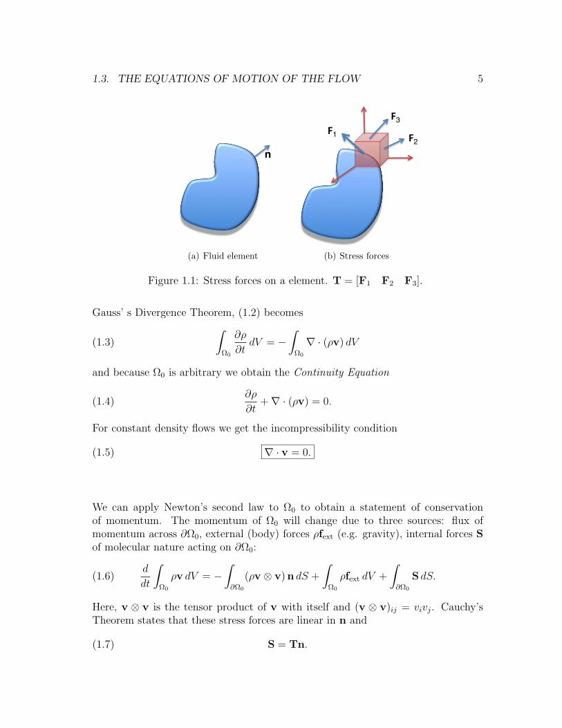
Consider an arbitrary fixed element of fluid Ω0 as in Fig. 1.1(a), with surface ∂Ω0.Then the rate of change of the total mass contained in that fluid element is equal tothe flux of mass across the surface ∂Ω0, in the absence of sinks or sources inside Ω0:

d

dt

∫Ω0

ρ dV = −∫∂Ω0

ρv · n dS.(1.2)

Here ρ is the mass density, v is the flow’s velocity field, and n is the unit normalpointing outward of ∂Ω0. This is the principle of conservation of mass. Using the

1.3. THE EQUATIONS OF MOTION OF THE FLOW 5

n!

!1!

!3!

!2!

(a) Fluid element

n!

!1!

!3!

!2!

(b) Stress forces

Figure 1.1: Stress forces on a element. T = [F1 F2 F3].

Gauss’ s Divergence Theorem, (1.2) becomes∫Ω0

∂ρ

∂tdV = −

∫Ω0

∇ · (ρv) dV(1.3)

and because Ω0 is arbitrary we obtain the Continuity Equation

∂ρ

∂t+∇ · (ρv) = 0.(1.4)

For constant density flows we get the incompressibility condition

∇ · v = 0.(1.5)

We can apply Newton’s second law to Ω0 to obtain a statement of conservationof momentum. The momentum of Ω0 will change due to three sources: flux ofmomentum across ∂Ω0, external (body) forces ρfext (e.g. gravity), internal forces Sof molecular nature acting on ∂Ω0:

d

dt

∫Ω0

ρv dV = −∫∂Ω0

(ρv ⊗ v) n dS +

∫Ω0

ρfext dV +

∫∂Ω0

S dS.(1.6)

Here, v ⊗ v is the tensor product of v with itself and (v ⊗ v)ij = vivj. Cauchy’sTheorem states that these stress forces are linear in n and

(1.7) S = Tn.


where T is a second order tensor called the stress tensor and we will represent it as amatrix. Thus, Tij is the i-th component of the force per unit area in a plane normalto the j-th direction (see Fig. 1.1(b)). Substituting (1.7 into (1.6) and applying theGauss’s Theorem we have∫

Ω0

∂(ρv)

∂tdV = −

∫Ω0

∇ · (ρv ⊗ v) dS +

∫Ω0

ρfext dV +

∫Ω0

∇ ·T dV.(1.8)

The divergence of the tensors ρv ⊗ v and T are the vectors with components

[∇ · (ρv ⊗ v)]i =3∑j=1

∂(ρvivj)

∂xj, (∇ ·T)i =

3∑j=1

∂Tij∂xj

,(1.9)

respectively. Thus, in differential form the conservation of momentum reads

∂(ρv)

∂t+∇ · (ρv ⊗ v) = ∇ ·T + ρfext.(1.10)

Upon using the Continuity Equation (1.4), we obtain the following equation in non-conservative form:

ρ

[∂v

∂t+ (v · ∇)v

]= ∇ ·T + ρfext,(1.11)

where

(v · ∇)vi =3∑j=1

vj∂vi∂xj

.(1.12)

The bracketed term in (1.11) is the material or substantial derivative of v :

Dv

Dt=∂v

∂t+ (v · ∇)v(1.13)

and thus the conservation of momentum can be written more succinctly as

(1.14) ρDv

Dt= ∇ ·T + ρfext.

Equations (1.5) and (1.14), supplemented with appropriate boundary and initialconditions, are the relevant equations to describe the motion of an incompressiblefluid. However, the system is not closed until we provide a mechanism to computethe stress tensor T. It is convenient to write T as

T = −pI + σ,(1.15)

1.3. THE EQUATIONS OF MOTION OF THE FLOW 7

where −pI represents the isotropic part due to hydrostatic pressure p and σ is thedeviatoric or excess stress. Often in continuum models of fluids, σ is taken to be afunction of the velocity gradient, σ = σ(∇v). Here, ∇v is the matrix given by

(∇v)ij =∂vi∂xj

.(1.16)

For a large class of fluids, so called Newtonian, σ obeys a simple constitutive equa-tion:

σ = µ(∇v +∇vT

)+

(κ− 2

3µ

)tr(∇v) I,(1.17)

where µ is the fluid viscosity, ∇vT denotes the transpose of the velocity gradient(1.16), κ is the dilatational viscosity, and tr(∇v) = ∇ · v is the trace of ∇v. Thus,for a Newtonian, incompressible fluid

T = −pI + µ(∇v +∇vT

).(1.18)

Often, in rheology literature ∇v denotes the transpose of (1.16). Here, we willretain the mathematical meaning given in (1.16) as the derivative matrix of v. Notethat with the constitutive equation for the stress, Eq. (1.18), we have a close systemgiven by (1.5), (1.14), (1.18). The system constitutes the Navier-Stokes equationsfor the dynamics of an incompressible Newtonian fluid.

It is convenient to decompose ∇v into its symmetric and anti-symmetric parts,∇v = D + Ω where

D =1

2

[∇v +∇vT

],(1.19)

Ω =1

2

[∇v −∇vT

].(1.20)

D is called the deformation or rate of strain tensor and Ω the vorticity tensor. Notethat tr(D) = ∇ · v and thus for an incompressible fluid D is traceless.

We are particularly interested in polymer solutions with an incompressible,Newtonian solvent. In such cases it is convenient to write the stress tensor as

(1.21) T = −pI + 2µD + σp,

where σp is the stress caused by the macromolecules.

The main task of the theory and of the computations of complexfluids is to obtain σp.

Like the Newtonian σ, the microstructural stress σp is symmetric for mostmodels. This follows from the assumption of isotropy (when the fluid is at rest) andthe conservation of angular momentum.


1.4 Creeping Flow: Stokes Approximation

In the absence of external forces, the Navier-Stokes equations (1.5), (1.14), and(1.18) for an incompressible, Newtonian fluid can be written as

ρ

(∂v

∂t+ v · ∇v

)= −∇p+ µ∇2v,(1.22)

∇ · v = 0.(1.23)

These equations may be non-dimensionalized by introducing a characteristic lengthscale Lc, a characteristic velocity Uc, and a characteristic time scale Tc. Let us selectTc = Lc/Uc. Introducing the following dimensionless variables

x′ =x

Lc,(1.24)

v′ =v

Uc,(1.25)

t′ =t(Lc

Uc

) ,(1.26)

p′ =p(µUc

Lc

) ,(1.27)

we get the non-dimensionalized Navier-Stokes equations:

Re

(∂v′

∂t′+ v′ · ∇′v′

)= −∇′p′ +∇′2v′,(1.28)

∇′ · v′ = 0,(1.29)

where

Re =ρUcLcµ

,(1.30)

is a dimensionless parameter known as the Reynolds number. Equations (1.28) and(1.29) as well as corresponding, non-dimensionalized boundary and initial conditionsdefine a one-parameter family of solutions (depending only on Re). All flows whichsatisfy the same non-dimensionalized boundary and initial conditions and whosecombination of µ, ρ, Lc, and Uc yield the same Re will be described by the samesolution of (1.28) and (1.29). This is the principle of Dynamic Similarity.

This Reynolds number can be interpreted as the ratio of inertial forces toviscous forces. Indeed

Re =

(ρU2

c

Lc

)(µUc

L2c

) .(1.31)

1.5. TWO IMPORTANT SIMPLE FLOWS 9

When inertial effects are small compared to viscous forces, i.e. Re 1, a usefulapproximation is to take formally the limit Re → 0 in the momentum equation(1.28). For these creeping flowsm we get the (steady) Stokes approximation:

−∇p+∇2v = 0,(1.32)

∇ · v = 0,(1.33)

where the primes have been dropped in all dimensionless variables to simplify thenotation.

For many complex fluid solutions Re 1 and thus it is appropriate to describetheir dynamics with the Stokes approximation. Going back to (1.14) and (1.21) andreintroducing the dimensioned variables we have the Stokes approximation for anincompressible, non-Newtonian solution:

−∇p+ µ∇2v +∇ · σp = 0,(1.34)

∇ · v = 0.(1.35)

Given the two-scale nature of complex fluids we call also speak of a microscopicReynolds number, Remicro. However, to maintain a separation of macro and microscales, we must assume that also Remicro 1 for otherwise the complex flow systemcould develop macroscopic boundary layers of characteristic length smaller than `.

1.5 Two Important Simple Flows

A simple shear flow is given by the velocity gradient

∇v =

0 γ 00 0 00 0 0

(1.36)

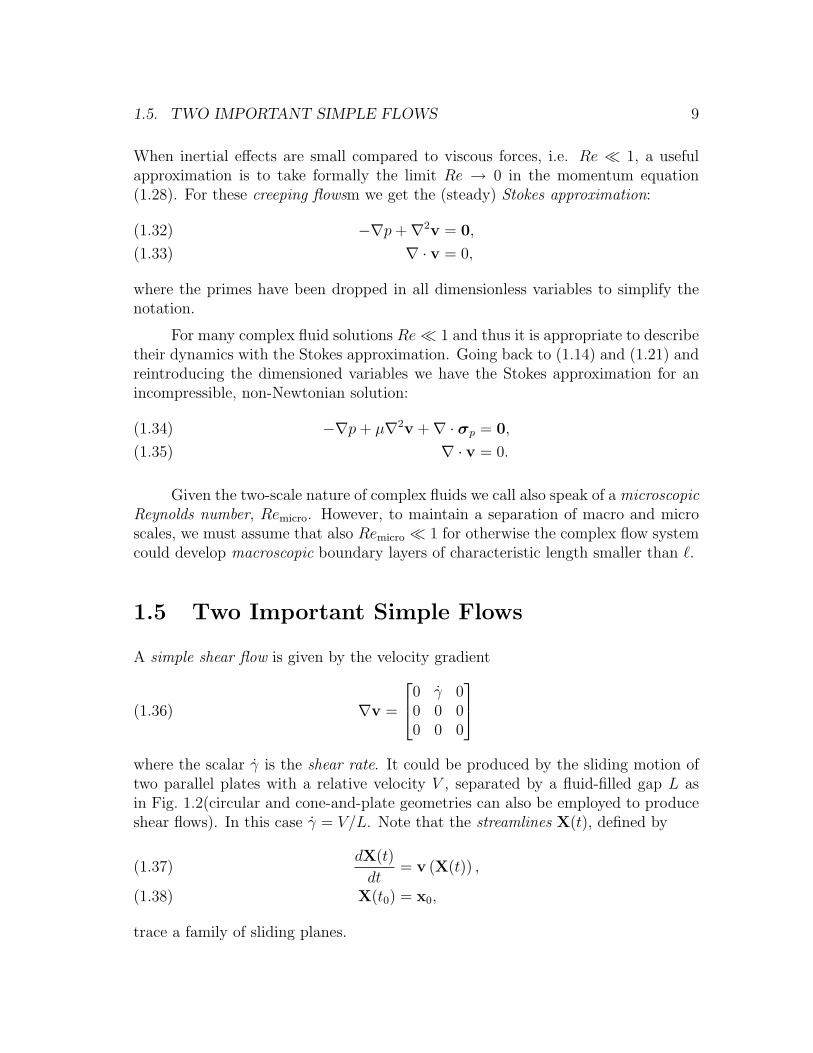
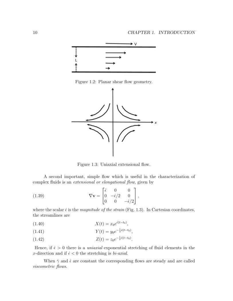
where the scalar γ is the shear rate. It could be produced by the sliding motion oftwo parallel plates with a relative velocity V , separated by a fluid-filled gap L asin Fig. 1.2(circular and cone-and-plate geometries can also be employed to produceshear flows). In this case γ = V/L. Note that the streamlines X(t), defined by

dX(t)

dt= v (X(t)) ,(1.37)

X(t0) = x0,(1.38)

trace a family of sliding planes.


!"

#"

Figure 1.2: Planar shear flow geometry.

!"

Figure 1.3: Uniaxial extensional flow.

A second important, simple flow which is useful in the characterization ofcomplex fluids is an extensional or elongational flow, given by

∇v =

ε 0 00 −ε/2 00 0 −ε/2

,(1.39)

where the scalar ε is the magnitude of the strain (Fig. 1.3). In Cartesian coordinates,the streamlines are

X(t) = x0eε(t−t0),(1.40)

Y (t) = y0e− 1

2ε(t−t0),(1.41)

Z(t) = z0e− 1

2ε(t−t0).(1.42)

Hence, if ε > 0 there is a uniaxial exponential stretching of fluid elements in thex-direction and if ε < 0 the stretching is bi-axial.

When γ and ε are constant the corresponding flows are steady and are calledviscometric flows.

1.6. MATERIAL FUNCTIONS 11

1.6 Material Functions

1.6.1 Shear Flows

In a shear flow of a Newtonian fluid only the shear stress σ12 = σ21 = µγ is non-zero.In general, for an isotropic, incompressible non-Newtonian fluid, the stress tensorhas the form

T =

−p+ σ11 σ12 0σ12 −p+ σ22 00 0 −p+ σ33

.(1.43)

The off-diagonal entries σ13 = σ31, and σ23 = σ32 are zero due to symmetry; arotation of π around the x3-axis leaves the velocity field invariant and assuming thefluid is isotropic the stress inherits this symmetry.

Because the pressure is defined up to an additive constant, only differences ofthe diagonal terms of T can be measured. Two such normal stress differences aredefined as:

N1 = σ11 − σ22,(1.44)

N2 = σ33 − σ22.(1.45)

Usually, N1 > 0 while N2 < 0 and |N2| < N1. For steady shear flow, i.e. γtime-independent, the shear viscosity η is defined, like in the Newtonian case, by

η(γ) =σ12(γ)

γ.(1.46)

Note that, in contrast to Newtonian fluids, the shear viscosity depends on the shearrate.

The normal stress differences N1 and N2 are also dependent on the shearrate, typically at a higher than linear rate. To characterize that dependence twoviscometric functions are defined as:

Ψ1(γ) =N1(γ)

γ2,(1.47)

Ψ2(γ) =N2(γ)

γ2.(1.48)

Ψ1 and Ψ2 are called the first and second normal stress coefficients. Note that for aNewtonian fluid both normal coefficients are zero.


In addition to steady flows, small amplitude shear flows are used experimen-tally to study the response of the microstructure to unsteady flows. In these non-steady flows the shear rate is sinusoidal:

γ(t) = γ0 cosωt,(1.49)

where γ0 1. Then, the stress varies also sinusoidal but not necessarily in phasewith the shear rate. This motion is expressed as

σ12 = γ0 [η′(ω) cosωt+ η′′(ω) sinωt] .(1.50)

This expression defines two viscosity functions η′ and η′′ or alternatively a “complex”viscosity function η∗ = η′−iη′′. Note that for a Newtonian fluid η′′ = 0. The functionη′ is called the dynamic viscosity. A complex modulus G∗ is defined through therelation G∗ = iωη∗ = G′ + iG′′. G′ and G′′ are called the loss modulus and storagemodulus, respectively.

1.6.2 Extensional Flows

Due to symmetry with respect to all the axes, the stress for simple extensional flowshas a very simple form:

T =

−p+ σ11 0 00 −p+ σ22 00 0 −p+ σ33

.(1.51)

Because the x2 and x3 directions are indistinguishable for this geometry, only thefirst normal stress difference N1 is relevant (N2 = 0). A viscosity function η(ε) isdefined to characterize the dependence of N1 on the magnitude of the strain ε forsteady flows:

η(ε) =N1(ε)

ε.(1.52)

1.7 Distinctive Phenomena in Complex Fluids

A characteristic feature of complex fluids under shear flows is that, in contrast toNewtonian fluids, the viscosity depends on the shear rate. For the majority ofcomplex fluids, the viscosity decreases with increasing shear rate. Fluids with thisbehavior are called shear thinning. Blood, paint, syrup, and molasses are familiarexamples of this type of non-Newtonian fluids. It is more unusual to have complex

1.7. DISTINCTIVE PHENOMENA IN COMPLEX FLUIDS 13

fluids whose viscosity increases with increasing shear rate. One example of this shearthickening fluid is quicksand (i.e. sand in water).

There are some complex fluids that would only start to flow for shear rateshigher than a certain threshold, like ketchup and toothpaste. These are called yieldfluids.

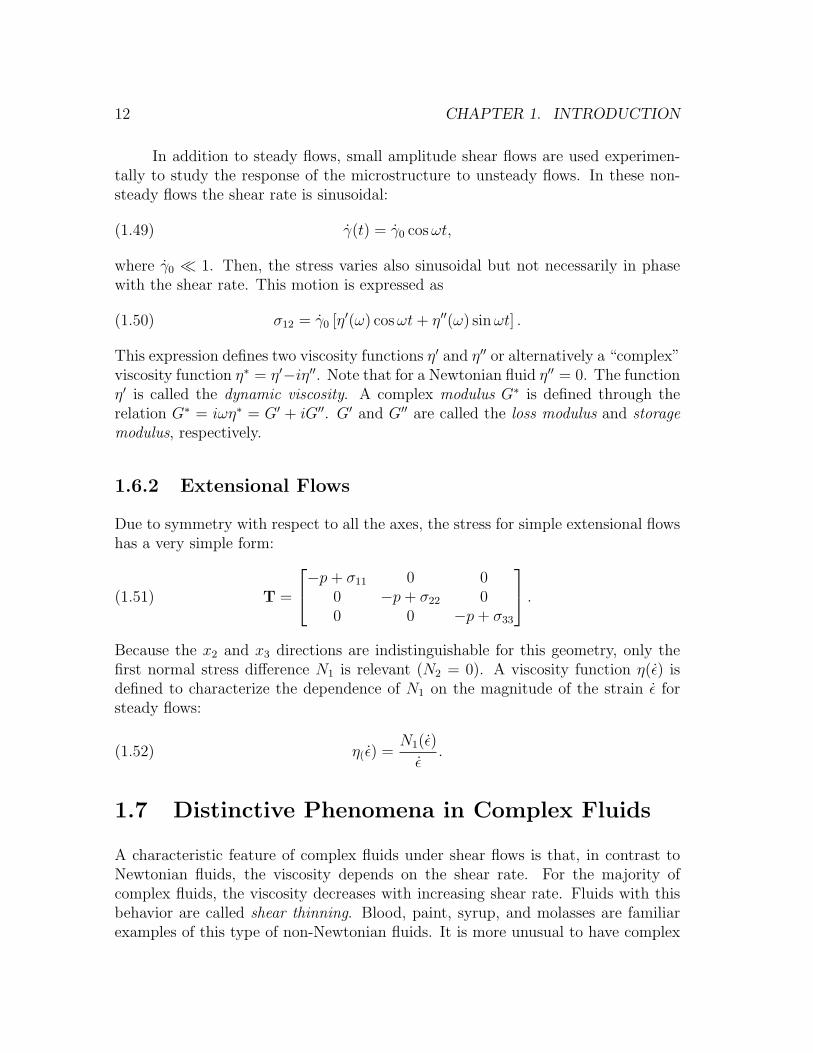
The imbedded microstructure interacting with the flow gives rise to a varietyof fascinating non-linear phenomena. Generally, there is a strong resistance of non-Newtonian fluid elements to stretching, i.e. a high extensional viscosity. As a result,even a few parts per million of polymers in a solution can lead to a strong inhibitionof drop break-up and jet formation which are important in several industrial appli-cations. This high resistance to stretching is also responsible for the cusp formationobserved at the trailing edge of an ascending bubble in a polymeric fluid to avoidthe large extensional flow flowing out of the rear stagnation point (see Fig. 1.4)

(a) (b) (c)

Figure 1.4: Ascending air bubble in (a) a Newtonian fluid and (b)-(c) a non-Newtonian fluid (front and side view) .

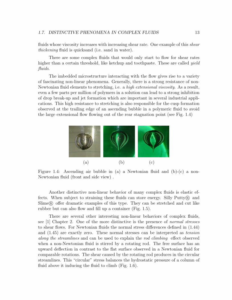
Another distinctive non-linear behavior of many complex fluids is elastic ef-fects. When subject to straining these fluids can store energy. Silly Putty R© andSlime R© offer dramatic examples of this type. They can be stretched and cut likerubber but can also flow and fill up a container (Fig. 1.5).

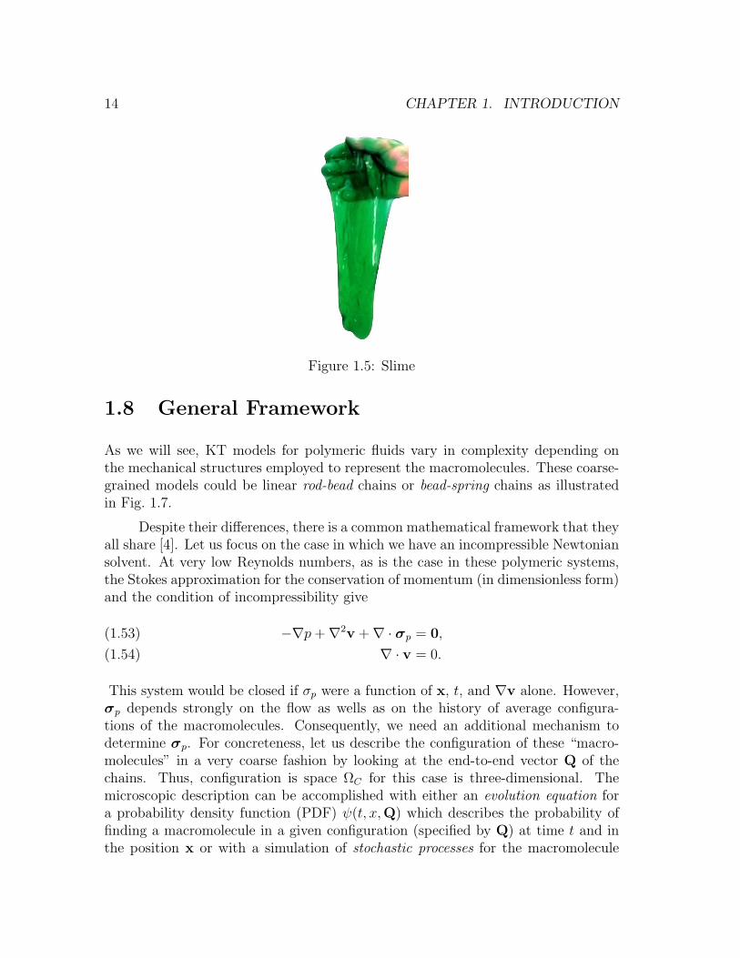
There are several other interesting non-linear behaviors of complex fluids,see [1] Chapter 2. One of the more distinctive is the presence of normal stressesto shear flows. For Newtonian fluids the normal stress differences defined in (1.44)and (1.45) are exactly zero. These normal stresses can be interpreted as tensionalong the streamlines and can be used to explain the rod climbing effect observedwhen a non-Newtonian fluid is stirred by a rotating rod. The free surface has anupward deflection in contrast to the flat surface observed in a Newtonian fluid forcomparable rotations. The shear caused by the rotating rod produces in the circularstreamlines. This “circular” stress balances the hydrostatic pressure of a column offluid above it inducing the fluid to climb (Fig. 1.6).


Figure 1.5: Slime

1.8 General Framework

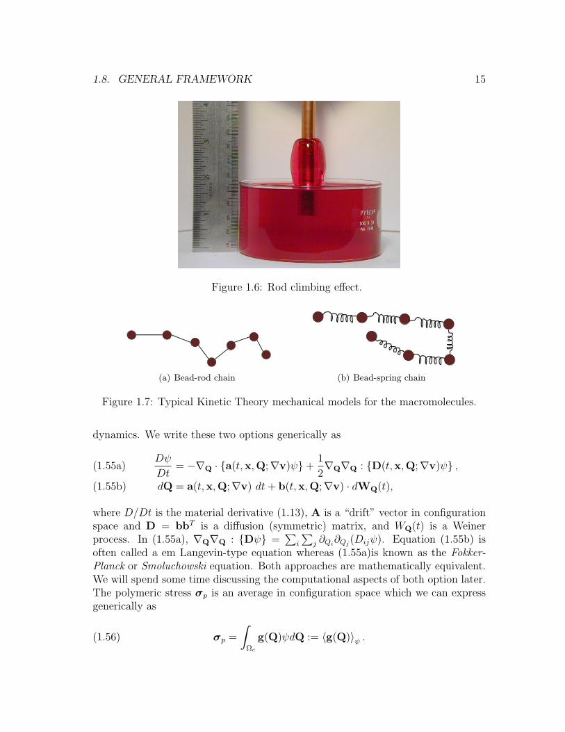
As we will see, KT models for polymeric fluids vary in complexity depending onthe mechanical structures employed to represent the macromolecules. These coarse-grained models could be linear rod-bead chains or bead-spring chains as illustratedin Fig. 1.7.

Despite their differences, there is a common mathematical framework that theyall share [4]. Let us focus on the case in which we have an incompressible Newtoniansolvent. At very low Reynolds numbers, as is the case in these polymeric systems,the Stokes approximation for the conservation of momentum (in dimensionless form)and the condition of incompressibility give

−∇p+∇2v +∇ · σp = 0,(1.53)

∇ · v = 0.(1.54)

This system would be closed if σp were a function of x, t, and ∇v alone. However,σp depends strongly on the flow as wells as on the history of average configura-tions of the macromolecules. Consequently, we need an additional mechanism todetermine σp. For concreteness, let us describe the configuration of these “macro-molecules” in a very coarse fashion by looking at the end-to-end vector Q of thechains. Thus, configuration is space ΩC for this case is three-dimensional. Themicroscopic description can be accomplished with either an evolution equation fora probability density function (PDF) ψ(t, x,Q) which describes the probability offinding a macromolecule in a given configuration (specified by Q) at time t and inthe position x or with a simulation of stochastic processes for the macromolecule

1.8. GENERAL FRAMEWORK 15

Figure 1.6: Rod climbing effect.

(a) Bead-rod chain (b) Bead-spring chain

Figure 1.7: Typical Kinetic Theory mechanical models for the macromolecules.

dynamics. We write these two options generically as

Dψ

Dt= −∇Q · a(t,x,Q;∇v)ψ+

1

2∇Q∇Q : D(t,x,Q;∇v)ψ ,(1.55a)

dQ = a(t,x,Q;∇v) dt+ b(t,x,Q;∇v) · dWQ(t),(1.55b)

where D/Dt is the material derivative (1.13), A is a “drift” vector in configurationspace and D = bbT is a diffusion (symmetric) matrix, and WQ(t) is a Weinerprocess. In (1.55a), ∇Q∇Q : Dψ =

∑i

∑j ∂Qi

∂Qj(Dijψ). Equation (1.55b) is

often called a em Langevin-type equation whereas (1.55a)is known as the Fokker-Planck or Smoluchowski equation. Both approaches are mathematically equivalent.We will spend some time discussing the computational aspects of both option later.The polymeric stress σp is an average in configuration space which we can expressgenerically as

σp =

∫Ωc

g(Q)ψdQ := 〈g(Q)〉ψ .(1.56)


The generic model (1.53)-(1.56) is deceivably simple. The devil is in the detailsand these will come from the particular KT mechanical models one employs todescribe the macromolecules. Even though these models are already coarse-grained,the large number of degrees of freedom makes this flow-structure interaction problema formidable computational challenge.

1.8.1 The Closure Problem

Alternatively, one could try to compute σp as follows. Assume σp = F(t,x; 〈QQ〉ψ).Multiply the Fokker-Plank equation (1.55a) by QQ and integrate with respect to Qin configuration space∫

ΩC

QQDψ

DtdQ = −

∫ΩC

QQ∇Q · a(t,x,Q;∇v)ψ dQ

+1

2

∫ΩC

QQ∇Q∇Q : D(t,x,Q;∇v)ψ(1.57)

The left hand side of (1.57) is just the material derivative of the second moment〈QQ〉ψ. However, the right hand side, with counted exceptions, will depend onhigher moments as well. Suppose it also depends on the fourth moment, so that(1.57) is an equation of the form

(1.58)D

Dt〈QQ〉ψ = G(t,x; 〈QQ〉ψ , 〈QQQQ〉ψ).

If we now derive an equation for the fourth moment its right hand side will depend onit and on the sixth moment as well. We have a closure problem. We are “mathemat-ically tempted” to approximate the high order moments using the low order ones.For example, we can postulate that 〈QQQQ〉ψ ≈ f(〈QQ〉ψ), for some “physicallyinspired” function f . Closure approximations are appealing because they reducethe dimensionality of the problem by eliminating the configuration space. However,the price paid can be substantial; a closure approximation can produce solutionsthat depart significantly from the expected physical behavior. Also troubling is thefact that closure approximations can change the type and structure of the coupledsystem of partial differential equations describing the flow-structure interaction.

1.9 Computational Challenges

In classical Computational Fluid Dynamics (CFD) of Newtonian flows we only needsto compute the velocity field v and the pressure p. In the computation of KT

1.9. COMPUTATIONAL CHALLENGES 17

models of complex fluids we must also compute the evolution of a microstructure.More precisely, at every in time and space (t,x) we need to evaluate the fluid stressinduced by the microstructure (macromolecules).

Computationally, it would be ideal if we had a time-evolution equation forthe stress σp, a so called constitutive equation, and solve this coupled to the Stokessystem (1.53)-(1.54) in our (t,x) computational domain. We could attempt to derivesuch an equation by getting evolution equations for the moments from (1.55a) asexplain in the preceding section. Unfortunately, only in very few simple cases ofKT models (Oldroyd B model being a notable example) can we obtain a closed,constitutive equation for σp. Hence, we are left to work with either (1.55b) or(1.55a). If we are inclined to work within a deterministic framework and use (1.55a)then we need to solve this equation in configuration space (i.e. in Q) for each point(t,x) of our computational time-space grid. Even in the simplest model of a rigid-likemolecule where need only need two degrees of freedom to describe its configuration(the angles of rotation, i.e configuration space is the unit sphere), the total numberof dimensions would be 1 + 3 + 2 = 6! Clearly, this approach quickly becomescomputationally intractable as the number of degrees of freedom to describe themacromolecules increases. The stochastic approach (1.55b) represents an attractivealternative to deal with such high dimensionality [6] but the overall flow-structureproblem is still a daunting challenge where significant advances in computationalmethodologies are much needed.

Bibliography

[1] R. B. Bird, C. F. Curtiss, R. C. Armstrong, and O. Hassager. Dynamics ofPolymeric Liquids. Volume 1: Fluid Mechanics. John Wiley and Sons, NewYork, 1987.

[2] R. B. Bird, C. F. Curtiss, R. C. Armstrong, and O. Hassager. Dynamics ofPolymeric Liquids. Volume 2: Kinetic Theory. John Wiley and Sons, New York,1987.

[3] M. Doi and S. F. Edwards. The Theory of Polymer Dynamics. Oxford UniversityPress, 1986.

[4] R. Keunings. Micro-macro methods for the multiscale simulation of viscoelasticflow using molecular models of kinetic theory. Rheology Reviews, pages 67–98,2004.

[5] R. G. Larson. The Structure and Rheology of Complex Fluids. Oxford UniversityPress, Oxford, 1999.

[6] H. C. Ottinger. Stochastic processes in polymeric fluids: tools and examples fordeveloping simulation algorithms. Springer, Berlin, 1996.

53

Notes on Complex Fluids: Kinetic Theory - UC Santa...

Documents

Transcript of Notes on Complex Fluids: Kinetic Theory - UC Santa...