Notes on Category Theory
416
Notes on Category Theory Robert L. Knighten November 9, 2007
Transcript of Notes on Category Theory

Notes on Category Theory
Robert L. Knighten
November 9, 2007

c© 2004–2007 by Robert L. KnightenAll rights reserved
Preface
There are many fine articles, notes, and books on category theory, so what isthe excuse for publishing yet another tome on the subject. My initial excusewas altruistic, a student asked for help in learning the subject and none ofthe available sources was quite appropriate. But ultimately I recognized thepersonal and selfish desire to produce my own exposition of the subject. Despitethat I have some hope that other students of the subject will find these notesuseful.
Target Audience & PrerequisitesCategory theory can sensibly be studied at many levels. Lawvere and
Schanuel in their book Conceptual Mathematics [47] have provided an intro-duction to categories assuming very little background in mathematics, whileMac Lane’s Categories for the Working Mathematician is an introduction tocategories for those who already have a substantial knowledge of other partsof mathematics. These notes are targeted to a student with significant “math-ematical sophistication” and a modest amount of specific knowledge. Thesophistication is primarily an ease with the definition-theorem-proof style ofmathematical exposition, being comfortable with an axiomatic approach, andfinding particular pleasure in exploring unexpected connections even with un-familiar parts of mathematics
Assumed Background: The critical specific knowledge assumed is a basicunderstanding of set theory. This includes such notions as subsets, unions andintersections of sets, ordered pairs, Cartesian products, relations, and functionsas relations. An understanding of particular types of functions, particularly bi-jections, injections, surjections and the associated notions of direct and inverseimages of subsets is also important. Other kinds of relations are importantas well, particularly equivalence relations and order relations. The basic ideasregarding finite and infinite sets, cardinal and ordinal numbers and inductionwill also be used.
All of this material is outlined in Appendix A on informal axiomatic settheory, but this is not likely to be useful as a first exposure to set theory.
Although not strictly required some minimal understanding of elementarygroup theory or basic linear algebra will certainly make parts of the text mucheasier to understand.
There are many examples scattered through the text which require someknowledge of other and occasionally quite advanced parts of mathematics. In
iii

iv PREFACE
particular Appendix B (Catalog of Categories) contains a discussion of a largevariety of specific categories. These typically assume some detailed knowledgeof some parts of mathematics. None of these examples are required for under-standing the body of the notes, but are included primarily for those readerswho do have such knowledge and secondarily to encourage readers to exploreother areas of mathematics.
Notation: The rigorous development of axiomatic set theory requires a veryprecise specification of the language and logic that is used. As part of that thereis some concise notation that has become common in much of mathematics andwhich will be used throughout these notes. Occasionally, often in descriptionsof sets, we will use various symbols from sentential logic particularly logicalconjunction ∧ for “and”, logical disjunction ∨ for “or”, implication ⇒ for“implies” and logical equivalence ⇐⇒ for “if and only if”. We also use ∀ and∃ from existential logic with ∀ meaning “for all” and ∃ meaning “there exists”.
Here is an example of the usage: For any sets A and B
∀A ∀B, A+B = x : (x ∈ A ∧ x /∈ B) ∨ (x /∈ A ∧ x ∈ B)
from which we conclude
∀A ∀B, A+B = A⇒ A ∩B = ∅
We have adopted two of Halmos’ fine notational conventions here as well:the use of “iff” when precision demands “if and only if” while felicity asks forless; and the end (or absence) of a proof is marked with .
Note on the ExercisesThere are 170 exercises in these notes, freely interspersed in the text. A list
of the exercises is included in the front matter, just after the list of definitions.Although the main purpose of the exercises is to develop your skill working withthe concepts and techniques of category theory, the results in the exercises arealso an integral part of our development. Solutions to all of the exercises areprovided in Appendix C, and you should understand them. If you have anydoubt about your own solution, you should read the solution in the Appendixbefore continuing on with the text. If you find an error in the text, in thesolutions, or just have a better solution, please send your comments to theauthor at [email protected]. They will be much appreciated.
Alternative SourcesThere are many useful accounts of the material in these notes, and the study
of category theory benefits from this variety of perspectives. In Appendix D areincluded brief reviews of the various books and notes, along with an indicationof their contents.
Throughout these Notes specific references are included for alternative dis-cussions of the material being treated, but no attempt has been made to provideattribution to original sources.

Contents
Preface iii
Contents v
List of Definitions xii
List of Exercises xix
Introduction 1
I Mathematics in Categories 3I.1 What is a Category? . . . . . . . . . . . . . . . . . . . . . . . 3
I.1.1 Hom and Related Notation . . . . . . . . . . . . . . . . 6I.1.2 Subcategories . . . . . . . . . . . . . . . . . . . . . . . 8I.1.3 Recognizing Categories . . . . . . . . . . . . . . . . . . 9
I.2 Special Morphisms . . . . . . . . . . . . . . . . . . . . . . . . 10I.2.1 Isomorphisms . . . . . . . . . . . . . . . . . . . . . . . 11I.2.2 Sections and Retracts . . . . . . . . . . . . . . . . . . . 12I.2.3 Epimorphisms and Monomorphisms . . . . . . . . . . . 13I.2.4 Subobjects and Quotient Objects . . . . . . . . . . . . 20
I.3 Special Objects . . . . . . . . . . . . . . . . . . . . . . . . . . 23I.3.1 Products and Sums . . . . . . . . . . . . . . . . . . . . 23I.3.2 Final, Initial and Zero Objects . . . . . . . . . . . . . 36I.3.3 Direct Sums and Matrices . . . . . . . . . . . . . . . . 39
I.4 Algebraic Objects . . . . . . . . . . . . . . . . . . . . . . . . . 46I.4.1 Magmas in a Category . . . . . . . . . . . . . . . . . . 47I.4.2 Comagmas in a Category . . . . . . . . . . . . . . . . . 50
I.4.2.1 Comagmas and Magmas Together . . . . . . . 53I.4.3 Monoids in a Category . . . . . . . . . . . . . . . . . . 56I.4.4 Comonoids in a Category . . . . . . . . . . . . . . . . . 61I.4.5 Groups in a Category . . . . . . . . . . . . . . . . . . . 64
II Constructing Categories 69II.1 Duality and Dual Category . . . . . . . . . . . . . . . . . . . . 69II.2 Quotient Categories . . . . . . . . . . . . . . . . . . . . . . . . 72
v

vi Contents
II.3 Product of Categories . . . . . . . . . . . . . . . . . . . . . . . 73II.4 Sum of Categories . . . . . . . . . . . . . . . . . . . . . . . . . 74II.5 Concrete and Based Categories . . . . . . . . . . . . . . . . . 74II.6 Morphism Categories . . . . . . . . . . . . . . . . . . . . . . . 76
III Functors and Natural Transformations 79III.1 What is a Functor? . . . . . . . . . . . . . . . . . . . . . . . . 79III.2 Examples of Functors . . . . . . . . . . . . . . . . . . . . . . . 82
III.2.1 Subcategories and Inclusion Functors . . . . . . . . . . 82III.2.2 Quotient Categories and Quotient Functors . . . . . . 82III.2.3 Product of Categories and Projection Functors . . . . 82III.2.4 Sum of Categories and Injection Functors . . . . . . . 83III.2.5 Constant Functors . . . . . . . . . . . . . . . . . . . . 84III.2.6 Forgetful Functors . . . . . . . . . . . . . . . . . . . . 85III.2.7 The Product Functor . . . . . . . . . . . . . . . . . . . 85III.2.8 The Sum Bifunctor . . . . . . . . . . . . . . . . . . . . 86III.2.9 Power Set Functor . . . . . . . . . . . . . . . . . . . . 86III.2.10 Monoid Homomorphisms are Functors . . . . . . . . . 86III.2.11 Forgetful Functor for Monoid . . . . . . . . . . . . . . 87III.2.12 Free Monoid Functor . . . . . . . . . . . . . . . . . . . 87III.2.13 Polynomial Ring as Functor . . . . . . . . . . . . . . . 88III.2.14 Commutator Functor . . . . . . . . . . . . . . . . . . . 88III.2.15 Abelianizer: Groups Made Abelian . . . . . . . . . . . 88III.2.16 Discrete Topological Space Functor . . . . . . . . . . . 89III.2.17 The Lie Algebra of a Lie Group . . . . . . . . . . . . . 90III.2.18 Homology Theory . . . . . . . . . . . . . . . . . . . . . 90
III.3 Categories of Categories . . . . . . . . . . . . . . . . . . . . . 90III.4 Digraphs and Free Categories . . . . . . . . . . . . . . . . . . 92III.5 Natural Transformations . . . . . . . . . . . . . . . . . . . . . 96III.6 Examples of Natural Transformations . . . . . . . . . . . . . . 98
III.6.1 Dual Vector Spaces . . . . . . . . . . . . . . . . . . . . 98III.6.2 Free Monoid Functor . . . . . . . . . . . . . . . . . . . 98III.6.3 Commutator and Abelianizer . . . . . . . . . . . . . . 99III.6.4 The Discrete Topology and the Forgetful Functor . . . 100III.6.5 The Godement Calculus . . . . . . . . . . . . . . . . . 101III.6.6 Functor Categories . . . . . . . . . . . . . . . . . . . . 102III.6.7 Examples of Functor Categories . . . . . . . . . . . . . 102III.6.8 Discrete Dynamical Systems . . . . . . . . . . . . . . . 104
IV Constructing Categories - Part II 107IV.1 Comma Categories . . . . . . . . . . . . . . . . . . . . . . . . 107
V Universal Mapping Properties 111V.1 Universal Elements . . . . . . . . . . . . . . . . . . . . . . . . 112V.2 Universal Arrows . . . . . . . . . . . . . . . . . . . . . . . . . 114V.3 Representable Functors . . . . . . . . . . . . . . . . . . . . . . 114

Contents vii
V.4 Initial and Final Objects . . . . . . . . . . . . . . . . . . . . . 115V.4.1 Free Objects . . . . . . . . . . . . . . . . . . . . . . . . 116
V.5 Limits and Colimits . . . . . . . . . . . . . . . . . . . . . . . . 117V.5.1 Cones and Limits . . . . . . . . . . . . . . . . . . . . . 121V.5.2 Cocones and Colimits . . . . . . . . . . . . . . . . . . . 130V.5.3 Complete Categories . . . . . . . . . . . . . . . . . . . 136
V.6 Adjoint Functors . . . . . . . . . . . . . . . . . . . . . . . . . 136V.7 Kan Extensions . . . . . . . . . . . . . . . . . . . . . . . . . . 145
V.7.1 Ends and Coends . . . . . . . . . . . . . . . . . . . . . 145
VI More Mathematics in a Category 147VI.1 Relations In Categories . . . . . . . . . . . . . . . . . . . . . . 147
VII Algebraic Categories 151VII.1 Universal Algebra . . . . . . . . . . . . . . . . . . . . . . . . . 152VII.2 Algebraic Theories . . . . . . . . . . . . . . . . . . . . . . . . 152VII.3 Internal Categories . . . . . . . . . . . . . . . . . . . . . . . . 152
VIII Cartesian Closed Categories 155VIII.1Partial Equivalence Relations and Modest Sets . . . . . . . . . 155
IX Topoi 161
X The Category of Sets Reconsidered 163
XI Monoidal Categories 165
XII Enriched Category Theory 167
XIII Additive and Abelian Categories 169
XIV Homological Algebra 171XIV.1 Introduction . . . . . . . . . . . . . . . . . . . . . . . . . . . . 171XIV.2 Additive Categories . . . . . . . . . . . . . . . . . . . . . . . . 171XIV.3 Abelian Categories . . . . . . . . . . . . . . . . . . . . . . . . 171XIV.4 Ext and Tor . . . . . . . . . . . . . . . . . . . . . . . . . . . . 171XIV.5 Category of Complexes . . . . . . . . . . . . . . . . . . . . . . 171XIV.6 Triangulated Categories . . . . . . . . . . . . . . . . . . . . . 171XIV.7 Derived Categories . . . . . . . . . . . . . . . . . . . . . . . . 171XIV.8 Derived Functors . . . . . . . . . . . . . . . . . . . . . . . . . 171
XV 2-Categories 173
XVI Fibered Categories 175
Appendices 177
A Set Theory 179

viii Contents
A.1 Extension Axiom . . . . . . . . . . . . . . . . . . . . . . . . . 180A.2 Axiom of Specification . . . . . . . . . . . . . . . . . . . . . . 181
A.2.1 Boolean Algebra of Classes . . . . . . . . . . . . . . . . 182A.3 Power-set Axiom . . . . . . . . . . . . . . . . . . . . . . . . . 185A.4 Axiom of Pairs . . . . . . . . . . . . . . . . . . . . . . . . . . . 186A.5 Union Axiom . . . . . . . . . . . . . . . . . . . . . . . . . . . 187A.6 Ordered Pairs and Cartesian Products . . . . . . . . . . . . . 188A.7 Relations . . . . . . . . . . . . . . . . . . . . . . . . . . . . . . 190A.8 Functions . . . . . . . . . . . . . . . . . . . . . . . . . . . . . . 194
A.8.1 Families and Cartesian Products . . . . . . . . . . . . 197A.8.2 Images . . . . . . . . . . . . . . . . . . . . . . . . . . . 199
A.9 Natural Numbers . . . . . . . . . . . . . . . . . . . . . . . . . 199A.10 Peano Axioms . . . . . . . . . . . . . . . . . . . . . . . . . . . 202A.11 Arithmetic . . . . . . . . . . . . . . . . . . . . . . . . . . . . . 206A.12 Order . . . . . . . . . . . . . . . . . . . . . . . . . . . . . . . . 209A.13 Number Systems . . . . . . . . . . . . . . . . . . . . . . . . . 213A.14 Axiom of Choice . . . . . . . . . . . . . . . . . . . . . . . . . . 216A.15 Zorn’s Lemma . . . . . . . . . . . . . . . . . . . . . . . . . . . 216A.16 Well Ordered Sets . . . . . . . . . . . . . . . . . . . . . . . . . 216A.17 Transfinite Induction . . . . . . . . . . . . . . . . . . . . . . . 216A.18 Axiom of Substitution . . . . . . . . . . . . . . . . . . . . . . 216A.19 Ordinal Numbers and Their Arithmetic . . . . . . . . . . . . . 217A.20 The Schroder-Bernstein Theorem . . . . . . . . . . . . . . . . 217A.21 Cardinal Numbers and Their Arithmetic . . . . . . . . . . . . 217A.22 Axiom of Regularity . . . . . . . . . . . . . . . . . . . . . . . 217
B Catalog of Categories 219B.1 Sets . . . . . . . . . . . . . . . . . . . . . . . . . . . . . . . . . 220
B.1.1 Set – sets . . . . . . . . . . . . . . . . . . . . . . . . . 220B.1.2 FiniteSet – finite sets . . . . . . . . . . . . . . . . . . 221B.1.3 Rel – the category of sets and relations . . . . . . . . 221B.1.4 RefRel – the category of sets and reflexive relations . 222B.1.5 SymRel – the category of sets and symmetric relations 222B.1.6 PSet – the category of sets and partial functions . . . 222B.1.7 Set∗ – the category of pointed sets . . . . . . . . . . . 222B.1.8 Ord – the category of ordinal numbers . . . . . . . . . 222
B.2 Semigroups, Monoids, Groups and Their Friends . . . . . . . . 222B.2.1 Magma – the category of magmas . . . . . . . . . . . 222B.2.2 Semigroup – the category of semigroups . . . . . . . 223B.2.3 Monoid – monoids . . . . . . . . . . . . . . . . . . . . 223B.2.4 CMonoid – commutative monoids . . . . . . . . . . . 226B.2.5 Group – groups . . . . . . . . . . . . . . . . . . . . . 227B.2.6 FiniteGroup – finite groups . . . . . . . . . . . . . . 228B.2.7 Ab – Abelian groups . . . . . . . . . . . . . . . . . . . 228
B.2.7.1 TorAb – Torsion Abelian groups . . . . . . . 228B.2.7.2 DivAb – Divisible Abelian groups . . . . . . . 228

Contents ix
B.2.7.3 TorsionFreeAb – Torsion Free Abelian groups 228B.3 Rings . . . . . . . . . . . . . . . . . . . . . . . . . . . . . . . . 228
B.3.1 Rig – rings without negatives . . . . . . . . . . . . . . 230B.3.2 Rng – rings without identity . . . . . . . . . . . . . . 231B.3.3 Ring – associative rings with identity . . . . . . . . . 231B.3.4 CommutativeRing – commutative rings . . . . . . . 232B.3.5 Field – fields . . . . . . . . . . . . . . . . . . . . . . . 232
B.4 Modules . . . . . . . . . . . . . . . . . . . . . . . . . . . . . . 232B.4.1 Module – modules over a commutative ring . . . . . . 232B.4.2 Matrices – matrices over a commutative ring . . . . . 232B.4.3 Vect – vector spaces . . . . . . . . . . . . . . . . . . . 233B.4.4 FDVect – finite dimensional vector spaces . . . . . . . 233
B.5 Algebras . . . . . . . . . . . . . . . . . . . . . . . . . . . . . . 233B.5.1 Algebra – associative algebras . . . . . . . . . . . . . 233B.5.2 LieAlgebra – Lie algebras . . . . . . . . . . . . . . . . 233
B.6 Order . . . . . . . . . . . . . . . . . . . . . . . . . . . . . . . . 234B.6.1 Preorder – preorders . . . . . . . . . . . . . . . . . . 234B.6.2 Poset – partially ordered sets . . . . . . . . . . . . . . 234B.6.3 Lattice – lattices . . . . . . . . . . . . . . . . . . . . . 234B.6.4 Full subcategories of equationally defined lattices . . . 237B.6.5 Boolean – the categories of Boolean algebras and Boolean
rings . . . . . . . . . . . . . . . . . . . . . . . . . . . . 238B.6.5.1 Boolean – the category of complete Boolean
algebras . . . . . . . . . . . . . . . . . . . . . . 242B.7 Ordered Algebraic Structures . . . . . . . . . . . . . . . . . . 242
B.7.1 OrderedMagma – Ordered Magmas . . . . . . . . . . 242B.7.2 OrderedMonoid – Ordered Monoids . . . . . . . . . 242B.7.3 OrderedGroup – Ordered Groups . . . . . . . . . . . 242B.7.4 OrderedRig – Ordered Rigs . . . . . . . . . . . . . . 243B.7.5 OrderedRing – Ordered Rings . . . . . . . . . . . . . 244
B.8 Graphs . . . . . . . . . . . . . . . . . . . . . . . . . . . . . . . 244B.8.1 Graph – graphs . . . . . . . . . . . . . . . . . . . . . 244B.8.2 Digraph – directed graphs . . . . . . . . . . . . . . . 245
B.9 Topology . . . . . . . . . . . . . . . . . . . . . . . . . . . . . . 245B.9.1 Metric – metric spaces . . . . . . . . . . . . . . . . . . 245B.9.2 Uniform – uniform spaces . . . . . . . . . . . . . . . . 245B.9.3 Top – topological spaces . . . . . . . . . . . . . . . . . 245B.9.4 Comp – compact Hausdorff spaces . . . . . . . . . . . 245B.9.5 Kspace – K-spaces . . . . . . . . . . . . . . . . . . . . 245B.9.6 Homotopy – the homotopy category of topological spaces245B.9.7 HSpace – H-Spaces . . . . . . . . . . . . . . . . . . . 246
B.10 Simplicial Categories . . . . . . . . . . . . . . . . . . . . . . . 246B.10.1 Simplicial – simplicial sets . . . . . . . . . . . . . . . 246B.10.2 Kan – the homotopy category of Kan complexes . . . 247
B.11 Differential, Graded and Filtered Algebraic Gadgets . . . . . . 247B.11.1 Graded Category . . . . . . . . . . . . . . . . . . . . . 247

x Contents
B.11.2 GradedModule . . . . . . . . . . . . . . . . . . . . . 247B.11.3 GradedRing . . . . . . . . . . . . . . . . . . . . . . . 247B.11.4 ChainComplex– Chain complexes . . . . . . . . . . . 248
B.12 Topological Algebras . . . . . . . . . . . . . . . . . . . . . . . 249B.12.1 TopGroup – topological groups . . . . . . . . . . . . 249B.12.2 TopAb – Abelian topological groups . . . . . . . . . . 249B.12.3 TopVect – topological vector spaces . . . . . . . . . . 249B.12.4 HausdorffTopVect – Hausdorff topological vector spaces249
B.13 Analysis . . . . . . . . . . . . . . . . . . . . . . . . . . . . . . 249B.13.1 Banach – Banach spaces . . . . . . . . . . . . . . . . . 249B.13.2 FDBanach – finite dimensional Banach spaces . . . . 249B.13.3 BanachAlgebra . . . . . . . . . . . . . . . . . . . . . 249
B.13.3.1 C*-algebra . . . . . . . . . . . . . . . . . . . . 249B.13.4 Hilbert – Hilbert spaces . . . . . . . . . . . . . . . . . 249B.13.5 FDHilb – finite dimensional Hilbert spaces . . . . . . 250
B.14 Differential Geometry . . . . . . . . . . . . . . . . . . . . . . . 250B.14.1 Manifold– smooth manifolds . . . . . . . . . . . . . . 250B.14.2 LieGroup– Lie groups . . . . . . . . . . . . . . . . . . 251
B.15 Algebraic and Analytic Geometry . . . . . . . . . . . . . . . . 251B.15.1 Sheaf . . . . . . . . . . . . . . . . . . . . . . . . . . . 251B.15.2 RingedSpace . . . . . . . . . . . . . . . . . . . . . . . 251B.15.3 Scheme – algebraic schemes . . . . . . . . . . . . . . . 251
B.16 Unusual Categories . . . . . . . . . . . . . . . . . . . . . . . . 252B.17 Cat – small categories . . . . . . . . . . . . . . . . . . . . . . 252B.18 Groupoid – groupoids . . . . . . . . . . . . . . . . . . . . . . 252B.19 Structures as Categories . . . . . . . . . . . . . . . . . . . . . 252
B.19.1 Every set is a category . . . . . . . . . . . . . . . . . . 252B.19.2 Every monoid is a category . . . . . . . . . . . . . . . 252B.19.3 Monoid of Strings . . . . . . . . . . . . . . . . . . . . . 252B.19.4 Every preorder is a category . . . . . . . . . . . . . . . 252B.19.5 Every topology is a category . . . . . . . . . . . . . . . 253
B.20 Little Categories . . . . . . . . . . . . . . . . . . . . . . . . . . 253B.20.1 0 – the empty category . . . . . . . . . . . . . . . . . . 253B.20.2 1 – the one morphism category . . . . . . . . . . . . . 253B.20.3 2 – the arrow category . . . . . . . . . . . . . . . . . . 254B.20.4 3 – the commutative triangle category . . . . . . . . . 254B.20.5 The parallel arrows category . . . . . . . . . . . . . . . 254
C Solutions of Exercises 255C.1 Solutions for Chapter I . . . . . . . . . . . . . . . . . . . . . . 256C.2 Solutions for Chapter II . . . . . . . . . . . . . . . . . . . . . 301C.3 Solutions for Chapter III . . . . . . . . . . . . . . . . . . . . . 303C.4 Solutions for Chapter IV . . . . . . . . . . . . . . . . . . . . . 315C.5 Solutions for Chapter V . . . . . . . . . . . . . . . . . . . . . 315C.6 Solutions for Chapter VII . . . . . . . . . . . . . . . . . . . . 316C.7 Solutions for Chapter VIII . . . . . . . . . . . . . . . . . . . . 316

Contents xi
C.8 Solutions for Chapter XIII . . . . . . . . . . . . . . . . . . . . 316C.9 Solutions for Chapter XIV . . . . . . . . . . . . . . . . . . . . 316C.10 Solutions for Chapter IX . . . . . . . . . . . . . . . . . . . . . 316C.11 Solutions for Chapter VI . . . . . . . . . . . . . . . . . . . . . 316C.12 Solutions for Appendix B . . . . . . . . . . . . . . . . . . . . . 316
D Other Sources 317D.1 Introductions . . . . . . . . . . . . . . . . . . . . . . . . . . . 318
D.1.1 Abstract and Concrete Categories: The Joy of Cats(Adamek, Herrlich, and Strecker [?]) . . . . . . . . . . 318
D.1.2 Category Theory (Awodey [?]) . . . . . . . . . . . . . . 318D.1.3 Category Theory: An Introduction (Herrlich and Strecker
[?]) . . . . . . . . . . . . . . . . . . . . . . . . . . . . . 320D.1.4 Arrows, Structures, and Functors: The Categorical Im-
perative (Arbib and Manes [1]) . . . . . . . . . . . . . 321D.1.5 Category Theory: Lecture Notes for ESSLLI (Barr and
Wells [?]) . . . . . . . . . . . . . . . . . . . . . . . . . . 321D.1.6 Category Theory for Computing Science (Barr and Wells
[3]) . . . . . . . . . . . . . . . . . . . . . . . . . . . . . 322D.1.7 Categories (Blyth [8]) . . . . . . . . . . . . . . . . . . . 324D.1.8 Handbook of Categorical Algebra I: Basic Category The-
ory (Borceux [?]) . . . . . . . . . . . . . . . . . . . . . 324D.1.9 Handbook of Categorical Algebra II: (Borceux [?]) . . 325D.1.10 Handbook of Categorical Algebra III: (Borceux [?]) . . 327D.1.11 Introduction to the Theory of Categories and Functors
(Bucur and Deleanu [?]) . . . . . . . . . . . . . . . . . 328D.1.12 Lecture Notes in Category Theory (Caccamo [?]) . . . 329D.1.13 Abelian Categories: An Introduction to the Theory of
Functors (Freyd [?]) . . . . . . . . . . . . . . . . . . . . 330D.1.14 A Categorical Primer (Hillman [?]) . . . . . . . . . . . 330D.1.15 An Introduction to Category Theory (Krishnan [?]) . . 331D.1.16 Conceptual Mathematics: A First Introduction to Cat-
egories (Lawvere and Schanuel [47]) . . . . . . . . . . . 331D.1.17 Theory of Categories (Mitchell [?]) . . . . . . . . . . . 334D.1.18 Categories and Functors (Pareigis [?]) . . . . . . . . . 336D.1.19 Theory of Categories (Popescu and Popescu [63]) . . . 336D.1.20 Categories (Schubert [?]) . . . . . . . . . . . . . . . . . 337D.1.21 Introduction to Category Theory and Categorical Logic
(Streichert [?]) . . . . . . . . . . . . . . . . . . . . . . . 340D.2 For Computer Science . . . . . . . . . . . . . . . . . . . . . . . 340
D.2.1 Categories, Types, and Structures: An Introduction toCategory Theory for the Working Computer Scientist(Asperti and Longo [?])) . . . . . . . . . . . . . . . . . 340
D.2.2 Categories for Types (Crole [?]) . . . . . . . . . . . . . 341D.2.3 A Gentle Introduction to Category Theory — The Cal-
culational Approach — (Fokkinga [?]) . . . . . . . . . 342

xii Contents
D.2.4 Basic Category Theory for Computer Scientists (Pierce[?]) . . . . . . . . . . . . . . . . . . . . . . . . . . . . . 342
D.2.5 Category Theory and Computer Programming (Pitt et.al. [?]) . . . . . . . . . . . . . . . . . . . . . . . . . . . 343
D.2.6 Categories and Computer Science (Walters [?]) . . . . 344D.3 Advanced - Specialized . . . . . . . . . . . . . . . . . . . . . . 344
D.3.1 Theory of Mathematical Structures (Adamek [?]) . . . 344D.3.2 Toposes, Triples, and Theories (Barr and Wells [?]) . . 345D.3.3 An Invitation to General Algebra and Universal Con-
structions (Bergman [?]) . . . . . . . . . . . . . . . . . 346D.3.4 Toposes and Local Set Theories (Bell [?]) . . . . . . . . 346D.3.5 Categories, Allegories (Freyd and Scedrov [25]) . . . . 347D.3.6 Topoi. The Categorical Analysis of Logic (Goldblatt [?]) 353D.3.7 Notes on Categories and Groupoids (Higgins[32]) . . . 354D.3.8 Topos Theory (Johnstone [?]) . . . . . . . . . . . . . . 355D.3.9 Sketches of an Elephant: a Topos Theory Compendium
(Johnstone [33, ?]) . . . . . . . . . . . . . . . . . . . . 356D.3.10 Categories and Sheaves (Kashiwara and Schapira [35]) 358D.3.11 Basic Concepts of Enriched Category Theory (Kelly [37])360D.3.12 Introduction to Higher Order Categorical Logic (Lam-
bek and Scott [?]) . . . . . . . . . . . . . . . . . . . . . 360D.3.13 Sets for Mathematics (Lawvere and Rosebrugh [46]) . . 361D.3.14 Categories for the Working Mathematician (Mac Lane
[53]) . . . . . . . . . . . . . . . . . . . . . . . . . . . . 362D.3.15 Sheaves in Geometry and Logic (Mac Lane and Mo-
erdijk [56]) . . . . . . . . . . . . . . . . . . . . . . . . . 363D.3.16 First Order Categorical Logic (Makkai and Reyes [?]) . 365D.3.17 Algebraic Theories (Manes [?]) . . . . . . . . . . . . . 366D.3.18 Elementary Categories, Elementary Toposes (McLarty
[?]) . . . . . . . . . . . . . . . . . . . . . . . . . . . . . 366D.3.19 Categorical Foundations (Pedicchio and Tholen [62] . . 368D.3.20 Introduction to Categories, Homological Algebra, and
Sheaf Cohomology (Strooker [?]) . . . . . . . . . . . . 369D.3.21 Practical Foundations of Mathematics (Taylor [?]) . . 370D.3.22 An Introduction to Homological Algebra (Weibel [65]) 371
Bibliography 375
Index 381

List of Definitions
I.1 category . . . . . . . . . . . . . . . . . . . . . . . . . . . . . . . . 3I.2 small category . . . . . . . . . . . . . . . . . . . . . . . . . . . . . 6I.3 large category . . . . . . . . . . . . . . . . . . . . . . . . . . . . . 6I.4 finite category . . . . . . . . . . . . . . . . . . . . . . . . . . . . . 6I.5 Hom . . . . . . . . . . . . . . . . . . . . . . . . . . . . . . . . . . 6I.6 locally small category . . . . . . . . . . . . . . . . . . . . . . . . 6I.7 f∗ . . . . . . . . . . . . . . . . . . . . . . . . . . . . . . . . . . . 8I.8 f∗ . . . . . . . . . . . . . . . . . . . . . . . . . . . . . . . . . . . 8I.9 endomorphism . . . . . . . . . . . . . . . . . . . . . . . . . . . . 8I.10 monoid of endomorphisms . . . . . . . . . . . . . . . . . . . . . . 8I.11 subcategory . . . . . . . . . . . . . . . . . . . . . . . . . . . . . . 8I.12 full subcategory . . . . . . . . . . . . . . . . . . . . . . . . . . . . 9I.13 isomorphism . . . . . . . . . . . . . . . . . . . . . . . . . . . . . . 11I.14 automorphism . . . . . . . . . . . . . . . . . . . . . . . . . . . . . 11I.15 automorphism group . . . . . . . . . . . . . . . . . . . . . . . . . 11I.16 groupoid . . . . . . . . . . . . . . . . . . . . . . . . . . . . . . . . 11I.17 section . . . . . . . . . . . . . . . . . . . . . . . . . . . . . . . . . 12I.18 retract . . . . . . . . . . . . . . . . . . . . . . . . . . . . . . . . . 12I.19 epimorphism . . . . . . . . . . . . . . . . . . . . . . . . . . . . . 14I.20 monomorphism . . . . . . . . . . . . . . . . . . . . . . . . . . . . 17I.21 bimorphism . . . . . . . . . . . . . . . . . . . . . . . . . . . . . . 19I.22 balanced category . . . . . . . . . . . . . . . . . . . . . . . . . . . 20I.23 subobject . . . . . . . . . . . . . . . . . . . . . . . . . . . . . . . 20I.24 equivalent subobjects . . . . . . . . . . . . . . . . . . . . . . . . . 20I.25 quotient object . . . . . . . . . . . . . . . . . . . . . . . . . . . . 21I.26 equivalent quotient objects . . . . . . . . . . . . . . . . . . . . . . 21I.27 product . . . . . . . . . . . . . . . . . . . . . . . . . . . . . . . . 23I.28 transposition (product) . . . . . . . . . . . . . . . . . . . . . . . . 27I.29 product of morphisms . . . . . . . . . . . . . . . . . . . . . . . . 27I.30 diagonal . . . . . . . . . . . . . . . . . . . . . . . . . . . . . . . . 29I.31 sum . . . . . . . . . . . . . . . . . . . . . . . . . . . . . . . . . . 29I.32 transposition (sum) . . . . . . . . . . . . . . . . . . . . . . . . . . 32I.33 sum of morphisms . . . . . . . . . . . . . . . . . . . . . . . . . . 32I.34 codiagonal . . . . . . . . . . . . . . . . . . . . . . . . . . . . . . . 34I.35 disjoint union . . . . . . . . . . . . . . . . . . . . . . . . . . . . . 34
xiii

xiv List of Definitions
I.36 final object . . . . . . . . . . . . . . . . . . . . . . . . . . . . . . 36I.37 point . . . . . . . . . . . . . . . . . . . . . . . . . . . . . . . . . . 36I.38 Cartesian category . . . . . . . . . . . . . . . . . . . . . . . . . . 37I.39 initial object . . . . . . . . . . . . . . . . . . . . . . . . . . . . . . 37I.40 co-Cartesian category . . . . . . . . . . . . . . . . . . . . . . . . 37I.41 zero object . . . . . . . . . . . . . . . . . . . . . . . . . . . . . . . 38I.42 zero morphism . . . . . . . . . . . . . . . . . . . . . . . . . . . . 38I.43 pointed set . . . . . . . . . . . . . . . . . . . . . . . . . . . . . . 38I.44 morphism of pointed sets . . . . . . . . . . . . . . . . . . . . . . 38I.45 join of pointed sets . . . . . . . . . . . . . . . . . . . . . . . . . . 38I.46 identity matrix . . . . . . . . . . . . . . . . . . . . . . . . . . . . 41I.47 direct sum . . . . . . . . . . . . . . . . . . . . . . . . . . . . . . . 42I.48 category with direct sums . . . . . . . . . . . . . . . . . . . . . . 42I.49 M . . . . . . . . . . . . . . . . . . . . . . . . . . . . . . . . . . . . 44I.50 O . . . . . . . . . . . . . . . . . . . . . . . . . . . . . . . . . . . . 44I.51 + . . . . . . . . . . . . . . . . . . . . . . . . . . . . . . . . . . . . 44I.52 sum of morphisms . . . . . . . . . . . . . . . . . . . . . . . . . . 46I.53 magma . . . . . . . . . . . . . . . . . . . . . . . . . . . . . . . . . 47I.54 magma homomorphism . . . . . . . . . . . . . . . . . . . . . . . . 47I.55 magma in a category . . . . . . . . . . . . . . . . . . . . . . . . . 47I.56 magma morphism . . . . . . . . . . . . . . . . . . . . . . . . . . . 48I.57 comagma . . . . . . . . . . . . . . . . . . . . . . . . . . . . . . . 50I.58 comagma morphism . . . . . . . . . . . . . . . . . . . . . . . . . 50I.59 monoid object . . . . . . . . . . . . . . . . . . . . . . . . . . . . . 56I.60 commutative monoid object . . . . . . . . . . . . . . . . . . . . . 57I.61 monoid morphism . . . . . . . . . . . . . . . . . . . . . . . . . . . 58I.62 comonoid . . . . . . . . . . . . . . . . . . . . . . . . . . . . . . . 61I.63 co-commutative comonoid . . . . . . . . . . . . . . . . . . . . . . 62I.64 comonoid morphism . . . . . . . . . . . . . . . . . . . . . . . . . 62I.65 group object . . . . . . . . . . . . . . . . . . . . . . . . . . . . . . 64I.66 group morphism . . . . . . . . . . . . . . . . . . . . . . . . . . . 65I.67 Abelian group object . . . . . . . . . . . . . . . . . . . . . . . . . 65II.1 dual category . . . . . . . . . . . . . . . . . . . . . . . . . . . . . 69II.2 congruence . . . . . . . . . . . . . . . . . . . . . . . . . . . . . . 72II.3 quotient category . . . . . . . . . . . . . . . . . . . . . . . . . . . 73II.4 product of two categories . . . . . . . . . . . . . . . . . . . . . . 73II.5 product of categories . . . . . . . . . . . . . . . . . . . . . . . . . 73II.6 sum of categories . . . . . . . . . . . . . . . . . . . . . . . . . . . 74II.7 concrete category - tentative . . . . . . . . . . . . . . . . . . . . . 74II.8 based category - tentative . . . . . . . . . . . . . . . . . . . . . . 75III.1 functor . . . . . . . . . . . . . . . . . . . . . . . . . . . . . . . . . 79III.2 contravariant functor . . . . . . . . . . . . . . . . . . . . . . . . . 79III.3 identity functor . . . . . . . . . . . . . . . . . . . . . . . . . . . . 80III.4 composition of functors . . . . . . . . . . . . . . . . . . . . . . . 80III.5 bifunctor . . . . . . . . . . . . . . . . . . . . . . . . . . . . . . . . 80III.6 isomorphism of categories . . . . . . . . . . . . . . . . . . . . . . 81

List of Definitions xv
III.7 full functor . . . . . . . . . . . . . . . . . . . . . . . . . . . . . . 81III.8 faithful functor . . . . . . . . . . . . . . . . . . . . . . . . . . . . 81III.9 inclusion functor . . . . . . . . . . . . . . . . . . . . . . . . . . . 82III.10 quotient functor . . . . . . . . . . . . . . . . . . . . . . . . . . . . 82III.11 projection functor . . . . . . . . . . . . . . . . . . . . . . . . . . . 82III.12 injection functor . . . . . . . . . . . . . . . . . . . . . . . . . . . 83III.13 constant functor . . . . . . . . . . . . . . . . . . . . . . . . . . . 84III.14 based category . . . . . . . . . . . . . . . . . . . . . . . . . . . . 85III.15 concrete category . . . . . . . . . . . . . . . . . . . . . . . . . . . 85III.16 Cat . . . . . . . . . . . . . . . . . . . . . . . . . . . . . . . . . . 90III.17 digraph . . . . . . . . . . . . . . . . . . . . . . . . . . . . . . . . 92III.18 digraph homomorphism . . . . . . . . . . . . . . . . . . . . . . . 92III.19 graph of a category . . . . . . . . . . . . . . . . . . . . . . . . . . 93III.20 path in a digraph . . . . . . . . . . . . . . . . . . . . . . . . . . . 93III.21 free category . . . . . . . . . . . . . . . . . . . . . . . . . . . . . 94III.22 natural transformation . . . . . . . . . . . . . . . . . . . . . . . . 96III.23 natural equivalence . . . . . . . . . . . . . . . . . . . . . . . . . . 97III.24 equivalence of categories . . . . . . . . . . . . . . . . . . . . . . . 97III.25 βF . . . . . . . . . . . . . . . . . . . . . . . . . . . . . . . . . . . 102III.26 Gα . . . . . . . . . . . . . . . . . . . . . . . . . . . . . . . . . . . 102III.27 C S . . . . . . . . . . . . . . . . . . . . . . . . . . . . . . . . . . . 102IV.1 comma category . . . . . . . . . . . . . . . . . . . . . . . . . . . . 107V.1 universal element . . . . . . . . . . . . . . . . . . . . . . . . . . . 112V.2 universal arrow . . . . . . . . . . . . . . . . . . . . . . . . . . . . 114V.3 representable functor . . . . . . . . . . . . . . . . . . . . . . . . . 114V.4 free object . . . . . . . . . . . . . . . . . . . . . . . . . . . . . . . 116V.5 pullback . . . . . . . . . . . . . . . . . . . . . . . . . . . . . . . . 118V.6 pushout . . . . . . . . . . . . . . . . . . . . . . . . . . . . . . . . 119V.7 cone . . . . . . . . . . . . . . . . . . . . . . . . . . . . . . . . . . 121V.8 limit . . . . . . . . . . . . . . . . . . . . . . . . . . . . . . . . . . 122V.9 kernel . . . . . . . . . . . . . . . . . . . . . . . . . . . . . . . . . 126V.10 normal monomorphism . . . . . . . . . . . . . . . . . . . . . . . . 127V.11 normal category . . . . . . . . . . . . . . . . . . . . . . . . . . . . 127V.12 parallel morphisms . . . . . . . . . . . . . . . . . . . . . . . . . . 128V.13 equalizer . . . . . . . . . . . . . . . . . . . . . . . . . . . . . . . . 128V.14 cocone . . . . . . . . . . . . . . . . . . . . . . . . . . . . . . . . . 130V.15 colimit . . . . . . . . . . . . . . . . . . . . . . . . . . . . . . . . . 131V.16 cokernel . . . . . . . . . . . . . . . . . . . . . . . . . . . . . . . . 133V.17 normal epimorphism . . . . . . . . . . . . . . . . . . . . . . . . . 134V.18 conormal category . . . . . . . . . . . . . . . . . . . . . . . . . . 134V.19 coequalizer . . . . . . . . . . . . . . . . . . . . . . . . . . . . . . 134V.20 complete category . . . . . . . . . . . . . . . . . . . . . . . . . . . 136V.21 cocomplete category . . . . . . . . . . . . . . . . . . . . . . . . . 136V.22 adjunction . . . . . . . . . . . . . . . . . . . . . . . . . . . . . . . 138VI.1 monic pair . . . . . . . . . . . . . . . . . . . . . . . . . . . . . . . 147VI.2 relation on object . . . . . . . . . . . . . . . . . . . . . . . . . . . 147

xvi List of Definitions
VI.3 reflexive relation . . . . . . . . . . . . . . . . . . . . . . . . . . . 148VI.4 symmetric relation . . . . . . . . . . . . . . . . . . . . . . . . . . 148VI.5 transitive relation . . . . . . . . . . . . . . . . . . . . . . . . . . . 148VI.6 equivalence relation (cats) . . . . . . . . . . . . . . . . . . . . . . 149VI.7 quotient modulo equivalence relation . . . . . . . . . . . . . . . . 149VI.8 regular monomorphism . . . . . . . . . . . . . . . . . . . . . . . . 149VI.9 extremal monomorphism . . . . . . . . . . . . . . . . . . . . . . . 149VII.1 internal category . . . . . . . . . . . . . . . . . . . . . . . . . . . 152VII.2 internal functor . . . . . . . . . . . . . . . . . . . . . . . . . . . . 152VII.3 internal natural transformation . . . . . . . . . . . . . . . . . . . 153VIII.1 partial equivalence relation . . . . . . . . . . . . . . . . . . . . . 155VIII.2 PER category . . . . . . . . . . . . . . . . . . . . . . . . . . . . . 157VIII.3 PER in a CCC . . . . . . . . . . . . . . . . . . . . . . . . . . . . 157VIII.4 PER category of a CCC . . . . . . . . . . . . . . . . . . . . . . . 158VIII.5 modest set . . . . . . . . . . . . . . . . . . . . . . . . . . . . . . . 158VIII.6 morphism of modest sets . . . . . . . . . . . . . . . . . . . . . . . 159IX.1 subobject classifier . . . . . . . . . . . . . . . . . . . . . . . . . . 161X.1 1 separates morphisms . . . . . . . . . . . . . . . . . . . . . . . . 163X.2 surjection (cat) . . . . . . . . . . . . . . . . . . . . . . . . . . . . 163A.1 set . . . . . . . . . . . . . . . . . . . . . . . . . . . . . . . . . . . 180A.2 proper class . . . . . . . . . . . . . . . . . . . . . . . . . . . . . . 180A.3 union . . . . . . . . . . . . . . . . . . . . . . . . . . . . . . . . . . 182A.4 intersection . . . . . . . . . . . . . . . . . . . . . . . . . . . . . . 182A.5 complement . . . . . . . . . . . . . . . . . . . . . . . . . . . . . . 183A.6 difference . . . . . . . . . . . . . . . . . . . . . . . . . . . . . . . 183A.7 union . . . . . . . . . . . . . . . . . . . . . . . . . . . . . . . . . . 183A.8 intersection . . . . . . . . . . . . . . . . . . . . . . . . . . . . . . 184A.9 subclass . . . . . . . . . . . . . . . . . . . . . . . . . . . . . . . . 184A.10 power set . . . . . . . . . . . . . . . . . . . . . . . . . . . . . . . 185A.11 singleton-class . . . . . . . . . . . . . . . . . . . . . . . . . . . . . 186A.12 pair . . . . . . . . . . . . . . . . . . . . . . . . . . . . . . . . . . 186A.13 symmetric difference . . . . . . . . . . . . . . . . . . . . . . . . . 187A.14 ordered pair . . . . . . . . . . . . . . . . . . . . . . . . . . . . . . 188A.15 Cartesian product . . . . . . . . . . . . . . . . . . . . . . . . . . 189A.16 relation-sets . . . . . . . . . . . . . . . . . . . . . . . . . . . . . . 190A.17 domain of definition . . . . . . . . . . . . . . . . . . . . . . . . . 190A.18 range . . . . . . . . . . . . . . . . . . . . . . . . . . . . . . . . . . 190A.19 reflexive . . . . . . . . . . . . . . . . . . . . . . . . . . . . . . . . 191A.20 symmetric . . . . . . . . . . . . . . . . . . . . . . . . . . . . . . . 191A.21 antisymmetric . . . . . . . . . . . . . . . . . . . . . . . . . . . . . 191A.22 connected . . . . . . . . . . . . . . . . . . . . . . . . . . . . . . . 191A.23 transitive . . . . . . . . . . . . . . . . . . . . . . . . . . . . . . . 191A.24 equivalence relation (sets) . . . . . . . . . . . . . . . . . . . . . . 191A.25 composition of relations . . . . . . . . . . . . . . . . . . . . . . . 192A.26 equivalence class . . . . . . . . . . . . . . . . . . . . . . . . . . . 192A.27 quotient set . . . . . . . . . . . . . . . . . . . . . . . . . . . . . . 193

List of Definitions xvii
A.28 disjoint . . . . . . . . . . . . . . . . . . . . . . . . . . . . . . . . . 193A.29 partition . . . . . . . . . . . . . . . . . . . . . . . . . . . . . . . . 193A.30 function . . . . . . . . . . . . . . . . . . . . . . . . . . . . . . . . 194A.31 general Cartesian product . . . . . . . . . . . . . . . . . . . . . . 198A.32 image . . . . . . . . . . . . . . . . . . . . . . . . . . . . . . . . . 199A.33 inverse image . . . . . . . . . . . . . . . . . . . . . . . . . . . . . 199A.34 zero . . . . . . . . . . . . . . . . . . . . . . . . . . . . . . . . . . 200A.35 successor of a set . . . . . . . . . . . . . . . . . . . . . . . . . . . 200A.36 natural numbers . . . . . . . . . . . . . . . . . . . . . . . . . . . 200A.37 sequence . . . . . . . . . . . . . . . . . . . . . . . . . . . . . . . . 201A.38 Peano system . . . . . . . . . . . . . . . . . . . . . . . . . . . . . 202A.39 transitive set . . . . . . . . . . . . . . . . . . . . . . . . . . . . . 205A.40 addition . . . . . . . . . . . . . . . . . . . . . . . . . . . . . . . . 206A.41 multiplication . . . . . . . . . . . . . . . . . . . . . . . . . . . . . 208A.42 exponent . . . . . . . . . . . . . . . . . . . . . . . . . . . . . . . . 208A.43 order in ω . . . . . . . . . . . . . . . . . . . . . . . . . . . . . . . 209A.44 preorder . . . . . . . . . . . . . . . . . . . . . . . . . . . . . . . . 209A.45 partial order . . . . . . . . . . . . . . . . . . . . . . . . . . . . . . 210A.46 strict order . . . . . . . . . . . . . . . . . . . . . . . . . . . . . . 210A.47 poset . . . . . . . . . . . . . . . . . . . . . . . . . . . . . . . . . . 210A.48 monotone . . . . . . . . . . . . . . . . . . . . . . . . . . . . . . . 211A.49 poset isomorphism . . . . . . . . . . . . . . . . . . . . . . . . . . 211A.50 total order . . . . . . . . . . . . . . . . . . . . . . . . . . . . . . . 211A.51 totally ordered set . . . . . . . . . . . . . . . . . . . . . . . . . . 211A.52 least element . . . . . . . . . . . . . . . . . . . . . . . . . . . . . 211A.53 greatest element . . . . . . . . . . . . . . . . . . . . . . . . . . . 212A.54 minimal element . . . . . . . . . . . . . . . . . . . . . . . . . . . 212A.55 maximal element . . . . . . . . . . . . . . . . . . . . . . . . . . . 212A.56 upper bound . . . . . . . . . . . . . . . . . . . . . . . . . . . . . 212A.57 lower bound . . . . . . . . . . . . . . . . . . . . . . . . . . . . . . 212A.58 least upper bound . . . . . . . . . . . . . . . . . . . . . . . . . . 212A.59 greatest lower bound . . . . . . . . . . . . . . . . . . . . . . . . . 213A.60 integers . . . . . . . . . . . . . . . . . . . . . . . . . . . . . . . . 215A.61 well ordered . . . . . . . . . . . . . . . . . . . . . . . . . . . . . . 216A.62 segment . . . . . . . . . . . . . . . . . . . . . . . . . . . . . . . . 216B.1 Set . . . . . . . . . . . . . . . . . . . . . . . . . . . . . . . . . . . 220B.2 partial function . . . . . . . . . . . . . . . . . . . . . . . . . . . . 222B.3 semigroup . . . . . . . . . . . . . . . . . . . . . . . . . . . . . . . 223B.4 commutative semigroup . . . . . . . . . . . . . . . . . . . . . . . 223B.5 monoid . . . . . . . . . . . . . . . . . . . . . . . . . . . . . . . . . 223B.6 monoid homomorphism . . . . . . . . . . . . . . . . . . . . . . . 224B.7 Monoid . . . . . . . . . . . . . . . . . . . . . . . . . . . . . . . . 224B.8 cancelable . . . . . . . . . . . . . . . . . . . . . . . . . . . . . . . 225B.9 invertible . . . . . . . . . . . . . . . . . . . . . . . . . . . . . . . 225B.10 commutative monoid . . . . . . . . . . . . . . . . . . . . . . . . . 226B.11 CMonoid . . . . . . . . . . . . . . . . . . . . . . . . . . . . . . . 226

xviii List of Definitions
B.12 group . . . . . . . . . . . . . . . . . . . . . . . . . . . . . . . . . 227B.13 group homomorphism . . . . . . . . . . . . . . . . . . . . . . . . 227B.14 category of groups . . . . . . . . . . . . . . . . . . . . . . . . . . 227B.15 Abelian group . . . . . . . . . . . . . . . . . . . . . . . . . . . . . 228B.16 ring . . . . . . . . . . . . . . . . . . . . . . . . . . . . . . . . . . 228B.17 rng . . . . . . . . . . . . . . . . . . . . . . . . . . . . . . . . . . . 229B.18 rig . . . . . . . . . . . . . . . . . . . . . . . . . . . . . . . . . . . 229B.19 rig homomorphism . . . . . . . . . . . . . . . . . . . . . . . . . . 230B.20 category of rigs . . . . . . . . . . . . . . . . . . . . . . . . . . . . 230B.21 rng homomorphism . . . . . . . . . . . . . . . . . . . . . . . . . . 231B.22 ring homomorphism . . . . . . . . . . . . . . . . . . . . . . . . . 231B.23 field . . . . . . . . . . . . . . . . . . . . . . . . . . . . . . . . . . 232B.24 module . . . . . . . . . . . . . . . . . . . . . . . . . . . . . . . . . 232B.25 algebra . . . . . . . . . . . . . . . . . . . . . . . . . . . . . . . . . 233B.26 lattice . . . . . . . . . . . . . . . . . . . . . . . . . . . . . . . . . 235B.27 lattice morphism . . . . . . . . . . . . . . . . . . . . . . . . . . . 235B.28 complete lattice . . . . . . . . . . . . . . . . . . . . . . . . . . . . 237B.29 distributive lattice . . . . . . . . . . . . . . . . . . . . . . . . . . 237B.30 modular lattice . . . . . . . . . . . . . . . . . . . . . . . . . . . . 238B.31 Boolean ring . . . . . . . . . . . . . . . . . . . . . . . . . . . . . . 238B.32 ordered magma . . . . . . . . . . . . . . . . . . . . . . . . . . . . 242B.33 ordered monoid . . . . . . . . . . . . . . . . . . . . . . . . . . . . 242B.34 ordered group . . . . . . . . . . . . . . . . . . . . . . . . . . . . . 242B.35 ordered rig . . . . . . . . . . . . . . . . . . . . . . . . . . . . . . . 243B.36 homomorphism of ordered rigs . . . . . . . . . . . . . . . . . . . 243B.37 category of ordered rig . . . . . . . . . . . . . . . . . . . . . . . . 243B.38 ordered ring . . . . . . . . . . . . . . . . . . . . . . . . . . . . . . 244B.39 graph . . . . . . . . . . . . . . . . . . . . . . . . . . . . . . . . . 244B.40 graph homomorphism . . . . . . . . . . . . . . . . . . . . . . . . 244B.41 digraph . . . . . . . . . . . . . . . . . . . . . . . . . . . . . . . . 245B.42 digraph homomorphism . . . . . . . . . . . . . . . . . . . . . . . 245B.43 graded category . . . . . . . . . . . . . . . . . . . . . . . . . . . . 247B.44 graded module . . . . . . . . . . . . . . . . . . . . . . . . . . . . 247B.45 graded ring . . . . . . . . . . . . . . . . . . . . . . . . . . . . . . 247B.46 associated ring . . . . . . . . . . . . . . . . . . . . . . . . . . . . 247B.47 chain complex . . . . . . . . . . . . . . . . . . . . . . . . . . . . . 248B.48 chain map . . . . . . . . . . . . . . . . . . . . . . . . . . . . . . . 248B.49 bounded chain complex . . . . . . . . . . . . . . . . . . . . . . . 248B.50 cycles . . . . . . . . . . . . . . . . . . . . . . . . . . . . . . . . . 248B.51 boundaries . . . . . . . . . . . . . . . . . . . . . . . . . . . . . . . 248B.52 acyclic . . . . . . . . . . . . . . . . . . . . . . . . . . . . . . . . . 248B.53 homology . . . . . . . . . . . . . . . . . . . . . . . . . . . . . . . 248B.54 chain homotopy . . . . . . . . . . . . . . . . . . . . . . . . . . . . 248B.55 Banach algebra . . . . . . . . . . . . . . . . . . . . . . . . . . . . 249B.56 inner product . . . . . . . . . . . . . . . . . . . . . . . . . . . . . 249B.57 presheaf . . . . . . . . . . . . . . . . . . . . . . . . . . . . . . . . 251

List of Definitions xix
B.58 ringed space . . . . . . . . . . . . . . . . . . . . . . . . . . . . . . 251

List of Exercises
I.1 (3 is a category) . . . . . . . . . . . . . . . . . . . . . . . . . . . 10I.2 (Is this a category?) . . . . . . . . . . . . . . . . . . . . . . . . 10I.3 (subcategory of surjections) . . . . . . . . . . . . . . . . . . . . 10I.4 (f isomorphism ⇒ f∗, f∗ isomorphisms) . . . . . . . . . . . . . 12I.5 (f∗ and f∗ isomorphisms ⇒ f an isomorphism) . . . . . . . . . 12I.6 (Isomorphism induces isomorphism of monoid of endomorphism) 12I.7 (Induced functions for sections and retracts) . . . . . . . . . . . 13I.8 (Section + retract ⇒ isomorphism) . . . . . . . . . . . . . . . . 13I.9 (Sections and retracts in Set) . . . . . . . . . . . . . . . . . . . 13I.10 (Has section ⇒ epimorphism) . . . . . . . . . . . . . . . . . . . 14I.11 (Epimorphisms induce injections) . . . . . . . . . . . . . . . . . 14I.12 (Epimorphisms may not induce surjections) . . . . . . . . . . . 14I.13 (Epimorphisms in N) . . . . . . . . . . . . . . . . . . . . . . . . 15I.14 (Epimorphisms in free monoid) . . . . . . . . . . . . . . . . . . 15I.15 (Epimorphisms in quotient monoid) . . . . . . . . . . . . . . . . 16I.16 (Has retract ⇒ monomorphism) . . . . . . . . . . . . . . . . . . 17I.17 (Monomorphisms induce injections) . . . . . . . . . . . . . . . . 17I.18 (Monomorphisms may not induce surjections) . . . . . . . . . . 17I.19 (Composition of retracts is retract) . . . . . . . . . . . . . . . . 18I.20 (Factor of retract is retract) . . . . . . . . . . . . . . . . . . . . 18I.21 (Composition of epimorphisms is epimorphism) . . . . . . . . . 18I.22 (Factor of epimorphism is epimorphism) . . . . . . . . . . . . . 18I.23 (Epimorphic section is isomorphism) . . . . . . . . . . . . . . . 18I.24 (Composition of sections is section) . . . . . . . . . . . . . . . . 19I.25 (Factor of section is section) . . . . . . . . . . . . . . . . . . . . 19I.26 (Composition of monomorphisms is monomorphism) . . . . . . 19I.27 (Factor of monomorphism is monomorphism) . . . . . . . . . . 19I.28 (Monomorphic retract is iso) . . . . . . . . . . . . . . . . . . . . 19I.29 (example of epimorphism that is not surjective) . . . . . . . . . 19I.30 (Give an example of a bimorphism) . . . . . . . . . . . . . . . . 19I.31 (mod f is an equivalence relation) . . . . . . . . . . . . . . . . . 22I.32 (f factors through B/f) . . . . . . . . . . . . . . . . . . . . . . . 22I.33 (Product in category of surjections) . . . . . . . . . . . . . . . . 25I.34 (Product of products is a product) . . . . . . . . . . . . . . . . 26I.35 (An object isomorphic to a product is a product) . . . . . . . . 27
xx

List of Exercises xxi
I.36 (A x B is isomorphic to B x A) . . . . . . . . . . . . . . . . . . 27I.37 (Permutation of product is isomorphic to product) . . . . . . . 27I.38 (Is a projection from a product necessarily an epimorphism?) . 27I.39 (f × g in Set) . . . . . . . . . . . . . . . . . . . . . . . . . . . . 28I.40 (Product of identities is identity) . . . . . . . . . . . . . . . . . 28I.41 (Composition of products is product of compositions) . . . . . . 28I.42 (Product of retracts is retract) . . . . . . . . . . . . . . . . . . . 28I.43 (Product of monomorphisms is monomorphism) . . . . . . . . . 28I.44 (Product of sections is a section) . . . . . . . . . . . . . . . . . 28I.45 (〈f, g〉h = 〈fh, gh〉) . . . . . . . . . . . . . . . . . . . . . . . . . 28I.46 (〈f, g〉 = (f × g)∆) . . . . . . . . . . . . . . . . . . . . . . . . . 29I.47 (∆ in Set) . . . . . . . . . . . . . . . . . . . . . . . . . . . . . . 29I.48 (∆ in Ab) . . . . . . . . . . . . . . . . . . . . . . . . . . . . . . 29I.49 (Sum of sums is a sum) . . . . . . . . . . . . . . . . . . . . . . . 32I.50 (An object isomorphic to a sum is a sum) . . . . . . . . . . . . 32I.51 (A+B is isomorphic to B+A) . . . . . . . . . . . . . . . . . . . 32I.52 (Permutation of sum is isomorphic to sum) . . . . . . . . . . . . 32I.53 (Does an injection into a sum have to be a monomorphism?) . . 32I.54 (Sum of identities is identity) . . . . . . . . . . . . . . . . . . . 33I.55 (Composition of sums is sum of compositions) . . . . . . . . . . 33I.56 (Sum of sections is a section) . . . . . . . . . . . . . . . . . . . 33I.57 (Sum of epimorphisms is epimorphism) . . . . . . . . . . . . . . 33I.58 (Sum of retracts is a retract) . . . . . . . . . . . . . . . . . . . . 33I.59 (Sum of monomorphisms need not be a monomorphism) . . . . 33I.60 (h[f, g] = [hf, hg]) . . . . . . . . . . . . . . . . . . . . . . . . . . 33I.61 ([f, g] = ∇(f + g)) . . . . . . . . . . . . . . . . . . . . . . . . . 34I.62 (f + g in Set) . . . . . . . . . . . . . . . . . . . . . . . . . . . . 35I.63 (Sum in Ab) . . . . . . . . . . . . . . . . . . . . . . . . . . . . 35I.64 (∇ in Ab) . . . . . . . . . . . . . . . . . . . . . . . . . . . . . . 35I.65 (f1 + f2 in Ab) . . . . . . . . . . . . . . . . . . . . . . . . . . . 35I.66 (Sum in Vect) . . . . . . . . . . . . . . . . . . . . . . . . . . . 35I.67 (∇ in Vect) . . . . . . . . . . . . . . . . . . . . . . . . . . . . . 35I.68 (f1 + f2 in Vect) . . . . . . . . . . . . . . . . . . . . . . . . . . 35I.69 (Final object is unique) . . . . . . . . . . . . . . . . . . . . . . . 36I.70 (Point of product is pair of points) . . . . . . . . . . . . . . . . 36I.71 (Final object x object = object) . . . . . . . . . . . . . . . . . . 36I.72 (points are subobjects) . . . . . . . . . . . . . . . . . . . . . . . 36I.73 (Initial object is unique) . . . . . . . . . . . . . . . . . . . . . . 37I.74 (Initial object + object = object) . . . . . . . . . . . . . . . . . 37I.75 (Matrix of morphisms) . . . . . . . . . . . . . . . . . . . . . . . 40I.76 (I in pointed sets) . . . . . . . . . . . . . . . . . . . . . . . . . . 41I.77 (Matrix of f+g) . . . . . . . . . . . . . . . . . . . . . . . . . . . 43I.78 (General matrix of product) . . . . . . . . . . . . . . . . . . . . 43I.79 (M and O in Ab) . . . . . . . . . . . . . . . . . . . . . . . . . . 44I.80 (f+0=f=0+f) . . . . . . . . . . . . . . . . . . . . . . . . . . . . 44I.81 (h(f + g) = hf + hg; (f + g)e = fe + ge) . . . . . . . . . . . . . 45

xxii List of Exercises
I.82 (ι1π1 + ι2π2 = 1A⊕A) . . . . . . . . . . . . . . . . . . . . . . . . 45I.83 (Category of magmas in a category) . . . . . . . . . . . . . . . 48I.84 (Magma category has finite products) . . . . . . . . . . . . . . . 49I.85 (Hom preserves magma morphisms) . . . . . . . . . . . . . . . . 49I.86 (h∗ is a magma homomorphism) . . . . . . . . . . . . . . . . . . 49I.87 (Category of comagmas in a category) . . . . . . . . . . . . . . 51I.88 (Homtakes comagma morphism to magma homomorphism) . . 51I.89 (h∗ is a magma homomorphism) . . . . . . . . . . . . . . . . . . 51I.90 (Comagma category has finite sums) . . . . . . . . . . . . . . . 52I.91 (Complete proof) . . . . . . . . . . . . . . . . . . . . . . . . . . 56I.92 (Category of monoids in a category) . . . . . . . . . . . . . . . 58I.93 (Category of commutative monoids in a category) . . . . . . . . 58I.94 (Monoid category has finite products) . . . . . . . . . . . . . . 59I.95 (Hom preserves monoid morphisms) . . . . . . . . . . . . . . . . 59I.96 (h∗ is a monoid homomorphism) . . . . . . . . . . . . . . . . . 59I.97 (Hom(•,M) commutative monoid ⇒ M commutative monoid) . 61I.98 (Category of comonoids in a category) . . . . . . . . . . . . . . 62I.99 (Category of co-commutative comonoids in a category) . . . . . 62I.100 (Comonoid category has finite sums) . . . . . . . . . . . . . . . 62I.101 (Hom takes comonoid morphisms to monoid homomorphisms) . 63I.102 (h∗ is a monoid homomorphism) . . . . . . . . . . . . . . . . . 63I.103 (Monoid Hom implies comonoid) . . . . . . . . . . . . . . . . . 64I.104 (Hom(A, •) commutative monoid ⇒ C co-commutative comonoid) 64I.105 (Category of groups in a category) . . . . . . . . . . . . . . . . 65I.106 (Category of Abelian groups in a category) . . . . . . . . . . . . 66I.107 (Group category has finite products) . . . . . . . . . . . . . . . 67I.108 (Verify ι∗ is inverse) . . . . . . . . . . . . . . . . . . . . . . . . 67I.109 (Hom preserves group morphisms) . . . . . . . . . . . . . . . . 67I.110 (h∗ is a group homomorphism) . . . . . . . . . . . . . . . . . . 67I.111 (Hom(•, G) a group implies G a group) . . . . . . . . . . . . . . 68II.1 (Quotient category is a category) . . . . . . . . . . . . . . . . . 73II.2 (product of two categories) . . . . . . . . . . . . . . . . . . . . . 73II.3 (sum of categories) . . . . . . . . . . . . . . . . . . . . . . . . . 74II.4 (concrete categories) . . . . . . . . . . . . . . . . . . . . . . . . 75II.5 (based categories) . . . . . . . . . . . . . . . . . . . . . . . . . . 75III.1 (Hom as bifunctor) . . . . . . . . . . . . . . . . . . . . . . . . . 81III.2 (Projection for product cat need not be full nor faithful) . . . . 83III.3 (Product with fixed object is functor) . . . . . . . . . . . . . . . 85III.4 (Sum with fixed object is functor) . . . . . . . . . . . . . . . . . 85III.5 (Sum is a bifunctor) . . . . . . . . . . . . . . . . . . . . . . . . 86III.6 (Product is a bifunctor) . . . . . . . . . . . . . . . . . . . . . . 86III.7 (Power set functor) . . . . . . . . . . . . . . . . . . . . . . . . . 86III.8 (Contravariant power set functor) . . . . . . . . . . . . . . . . . 86III.9 (Forgetful functor for monoid category) . . . . . . . . . . . . . . 87III.10 (f∗ is a monoid homomorphism) . . . . . . . . . . . . . . . . . 87III.11 (Free monoid as adjoint) . . . . . . . . . . . . . . . . . . . . . . 88

List of Exercises xxiii
III.12 (Polynomial ring functor) . . . . . . . . . . . . . . . . . . . . . 88III.13 (Commutator functor) . . . . . . . . . . . . . . . . . . . . . . . 88III.14 (G/[G,G] as functor) . . . . . . . . . . . . . . . . . . . . . . . . 89III.15 (Abelianizer as adjoint) . . . . . . . . . . . . . . . . . . . . . . . 89III.16 (Discrete topology adjoint to forgetful) . . . . . . . . . . . . . . 89III.17 (f is a functor) . . . . . . . . . . . . . . . . . . . . . . . . . . . 94III.18 (Free category as adjoint) . . . . . . . . . . . . . . . . . . . . . 94III.19 (Describe F (U(2)) // 2) . . . . . . . . . . . . . . . . . . . . . 96III.20 (Describe free category of non-category digraph) . . . . . . . . 96III.21 (natural transformation of constant functors) . . . . . . . . . . 97III.22 (V // V ∗∗ is natural) . . . . . . . . . . . . . . . . . . . . . . . 98III.23 (1 // UF is a natural transformation) . . . . . . . . . . . . . 98III.24 (FU // 1 is a natural transformation) . . . . . . . . . . . . . 99III.25 (ε gives adjunction) . . . . . . . . . . . . . . . . . . . . . . . . . 99III.26 (η gives adjunction) . . . . . . . . . . . . . . . . . . . . . . . . . 99III.27 (Monoid(F (•), •) is naturally equivalent to Set(•, U(•))) . . . 99III.28 (Commutator // 1Group is a natural transformation) . . . . . 99III.29 (1Group
// IA is a natural transformation) . . . . . . . . . . 100III.30 (Ab(A(G), A) // Group(G, I(A))) . . . . . . . . . . . . . . . 100III.31 (Ab(A(•), •) is naturally equivalent to Group(•, I(•))) . . . . 100III.32 (FU // 1Top is a natural transformation) . . . . . . . . . . . 101III.33 (Top(F (S), X) ∼= Set(S,U(X))) . . . . . . . . . . . . . . . . . 101III.34 (Top(F (•), •) is naturally isomorphic to Set(•, U(•))) . . . . . 101III.35 (βF is a natural transformation) . . . . . . . . . . . . . . . . . 102III.36 (Gα is a natural transformation) . . . . . . . . . . . . . . . . . 102III.37 (C 1 ∼= C ) . . . . . . . . . . . . . . . . . . . . . . . . . . . . . . 102III.38 (C n) . . . . . . . . . . . . . . . . . . . . . . . . . . . . . . . . . 103IV.1 (universal mapping property of comma categories) . . . . . . . 110V.1 (pullbacks in Set) . . . . . . . . . . . . . . . . . . . . . . . . . . 119V.2 (Example of monomorphism not a kernel) . . . . . . . . . . . . 127V.3 (pullback as equalizer) . . . . . . . . . . . . . . . . . . . . . . . 130V.4 (Example of epimorphism not a cokernel) . . . . . . . . . . . . 133V.5 (Complete proof of θξ = 1) . . . . . . . . . . . . . . . . . . . . . 144VI.1 (jointly monic) . . . . . . . . . . . . . . . . . . . . . . . . . . . 147VI.2 (Hom preserves and reflects reflexive relations) . . . . . . . . . 148VI.3 (Hom preserves and reflects symmetric relations) . . . . . . . . 148VI.4 (Hom preserves and reflects transitive relations) . . . . . . . . . 148VIII.1 (PER=PER(Set)) . . . . . . . . . . . . . . . . . . . . . . . . . . 158IX.1 (characteristic function) . . . . . . . . . . . . . . . . . . . . . . 161IX.2 (equivalent subobjects) . . . . . . . . . . . . . . . . . . . . . . . 162IX.3 (unique subobject classifier) . . . . . . . . . . . . . . . . . . . . 162B.1 (Describe categories arising from preorders) . . . . . . . . . . . 252B.2 (Product and sum in 2) . . . . . . . . . . . . . . . . . . . . . . 254


Introduction
Over the past century much of the progress in mathematics has been due togeneralization and abstraction. Groups arose largely from the study of sym-metries in various contexts, and group theory came when it was realized thatthere was a general abstraction that captured ideas that were being developedseparately. Similarly linear algebra arose initially by recognizing the commonground under the development of linear equations, matrices, determinants andother notions. Then as linear algebra was codified it was recognized that itapplied to very different situations and so, for example, its relevance to func-tional analysis was recognized and powerfully shaped the development of thatfield.
Topology, as the study of topological spaces, began around the middle ofthe 19th century. What we now call Algebraic Topology largely began with thework in Poincare’s series of papers called Complents a l’Analysis Situs whichhe began publishing in 1895. Over the next 30 years Algebraic Topology de-veloped rather slowly, but this was the same time that abstract algebra aswas coming into being (as exemplified by van der Waerden’s still well-namedModerne Algebra published in 1931.) About 1925 homology groups began toappear in all of their glory, and over the next twenty years much of the basicsof modern algebraic topology appeared. But a basic insight was still missing– the recognition that in algebraic topology the important operations not onlyassign groups to topological spaces but also assign group homomorphisms tothe continuous maps between the spaces. Indeed in order to axiomatize homol-ogy and cohomology theory the notion of equivalence between such operationswas also needed. That was provided by Eilenberg and Mac Lane in theirground breaking paper “General theory of natural equivalences” [20], wherethe definitions of categories, functors and natural equivalences were first given.(A very good and extensive book on all of this and a very great deal more isDieudonne’s A History of Algebraic and Differential Topology 1900-1960 [15].)
X
1


Chapter I
Mathematics in Categories
I.1 What is a Category?
Definition I.1: A category C has objects A,B,C, · · · , P,Q, . . . , and mor-phisms f, g, h, i, · · · , x, y, · · · . To each morphism is associated two objects, itsdomain and codomain. If f is a morphism with domain A and codomain B,this is indicated by f : A // B. Each object, A, has an associated identitymorphism written 1A : A // A. Finally if f : A // B and g : B // C,there is a composition gf : A // C, and these all satisfy the following rela-tions:
1. (Associativity) If f : A // B, g : B // C and h : C // D, thenh(gf) = (hg)f : A // D.
2. (Identity Morphisms) If f : A // B, then f1A = f = 1Bf .
Sometimes gf is unclear and g f will be used instead. These are both readas “f composed with g” or as “g following f”.
Relations such as these are indicated by saying diagrams of the followingsort commute, meaning that any sequence of compositions of morphisms in thediagram that start and end at the same nodes in the diagram are equal.
1.
A
Bf
??A
C
gf
????????
B
C
g
B
D
hg
????????
C
D
h
??
3

4 CHAPTER I. MATHEMATICS IN CATEGORIES
2.
A A1A //A
B
f
??????????????A
B
f
''OOOOOOOOOOOOOOOOOOOOOOOO A
B
f
??????????????
B B1B //
For example in diagram (1.) commutativity of the left triangle says that gfis the g following f and the left triangle says that hg is h following g, whichis certainly true but just the meaning of gf and hg. More interesting the topcomposite, (hg)f , is equal to the bottom composite, h(gf), which is exactlyAssociativity. There is also h following g following f , and what Associativityallows us to say is that this is equal to both (hg)f and h(gf), i.e., the ordermatters, but parenthesis are unneeded.
In diagram (2.), commutativity of the top triangle says f1A is equal to f,while commutativity of the lower triangle say f if equal to 1Bf . And these areexactly the requirements on the identify morphisms.
Note: Because category theory is applicable to so many diverse areas whichhave their own terminology, often well established before categories intruded, itis common even when discussing category theory to use a variety of terminology.For example while morphism is the most commonly used term, these elementsof a category are also called “maps”,and sometimes “arrows”.Indeed we willoccasionally use the word “map” as a synonym for morphism. Similarly whatwe called the domain of a morphism is sometimes called the “source”,while“target”is an alternative for codomain.
Note: Throughout these notes script capital letters such as A , B, C , . . . ,X , Y , Z will be used without further comment to denote categories.
Examples of categories, familiar and unfamiliar, are readily at hand, butrather than listing them here Appendix B provides a Catalog of Categorieswhere many examples are listed, together with detailed information about eachof them. Each time a new concept or theorem appears it will be worthwhile tobrowse that Appendix for relevant examples.
There are two extreme examples of categories that are worthy of mentionhere. The first is the category Set of sets. Set has as objects all sets, andas morphisms all functions between sets. (For details see Section B.1.1 in theCatalog of Categories.) It is common in the development of the theory of setsto identify a function with its graph as a subset of the Cartesian product of itsdomain and its codomain. (See definition A.30 in Section A.8.) One result ofthis is that from the function (considered just as a set) it is possible to recoverthe domain of the function, but not in general its codomain. So when we saythe morphisms are “all functions between sets” we actually consider a functionas including a specification of its codomain. This same remark applies to manyof the other “familiar” categories that we consider such as the categories ofgroups, Abelian groups, vector spaces, topological spaces, manifolds, etc.

I.1. WHAT IS A CATEGORY? 5
By contrast suppose that (M,µ) is a monoid, that is a set M together anassociative binary operation on M that has identity element (which we call 1.)Using M we define a category M which has only one object, which has M asits set of morphisms, all with the one object as both domain and codomain,with the identity of the monoid as the identity morphism on the unique object,and composition defined by the multiplication µ. We will usually refer to thecategory M by writing “consider the monoid M as a category with one object”without using any special name.
Conversely if C is any category with only one object, the morphisms withcomposition as multiplication form a monoid – save for one significant caveat,the definition of a monoid stipulates that M is a set.
For more information on monoids, look at the material in Section B.2.3 ofthe Catalog of Categories.
Our basic reference for topics in algebra is Mac Lane and Birkhoff’s Alge-bra [55]. In particular for the definition and basic properties of a monoid see[55, I.11].
As an algebraic gadget the expected definition of a category is probablysomething like: A category, C , consists of two sets Objects and Morphismsand functions:
domain : Morphisms // Objects,codomain : Morphisms // Objects,
id : Objects // Morphisms
and a partial function
composition : Morphisms×Morphisms // Morphisms
such that . . . .The reason the definition we’ve given makes no mention of sets at all is
because the most familiar categories, such as Set, do not have either a set ofobjects or a set of morphisms.
The connection between set theory and category theory is an odd one.Exactly how category theory should be explained in terms of set theory is stilla topic of controversy, while at the same time most writers on either set theoryor category theory give the subject scant attention. And that is what we willdo as well. For those who are interested in more information about these issues,consult [50], [51] and [24] as a start.
There is also an active effort to use category theory as alternative founda-tion for set theory or even all of mathematics. Some references for these topicsinclude Lawvere’s “An Elementary Theory of the Category of Sets” [41, 44]and “The category of categories as a foundation for mathematics” [42], a cou-ple of efforts to correct some errors, “Lawvere’s basic theory of the category ofcategories” [7, 6]. A later discussion of axiomatizing the category of categoriesis McLarty’s “Axiomatizing a Category of Categories” [57] , and a later dis-cussion of axiomatizing the category of sets is Osius’ “Categorical Set Theory:a Characterisation of the Category of Sets” [60].
6 CHAPTER I. MATHEMATICS IN CATEGORIES
With the arrival of the theory of topoi, that became the most importanttool for discussing category theory and foundations. See Joyal and Moerdijk,[34], Mac Lane and Moerdijk, [56] and Lawvere and Rosebrugh [46] .
After that digression, we make the following definitions.
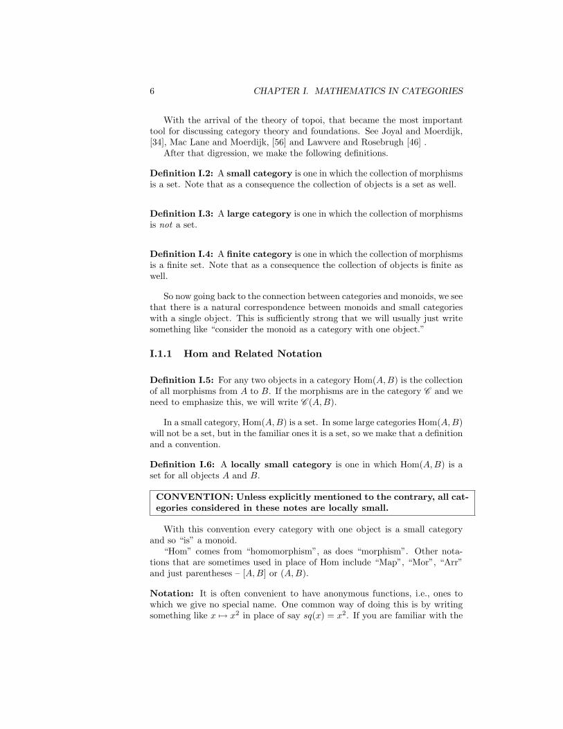
Definition I.2: A small category is one in which the collection of morphismsis a set. Note that as a consequence the collection of objects is a set as well.
Definition I.3: A large category is one in which the collection of morphismsis not a set.
Definition I.4: A finite category is one in which the collection of morphismsis a finite set. Note that as a consequence the collection of objects is finite aswell.
So now going back to the connection between categories and monoids, we seethat there is a natural correspondence between monoids and small categorieswith a single object. This is sufficiently strong that we will usually just writesomething like “consider the monoid as a category with one object.”
I.1.1 Hom and Related Notation
Definition I.5: For any two objects in a category Hom(A,B) is the collectionof all morphisms from A to B. If the morphisms are in the category C and weneed to emphasize this, we will write C (A,B).
In a small category, Hom(A,B) is a set. In some large categories Hom(A,B)will not be a set, but in the familiar ones it is a set, so we make that a definitionand a convention.
Definition I.6: A locally small category is one in which Hom(A,B) is aset for all objects A and B.
CONVENTION: Unless explicitly mentioned to the contrary, all cat-egories considered in these notes are locally small.
With this convention every category with one object is a small categoryand so “is” a monoid.
“Hom” comes from “homomorphism”, as does “morphism”. Other nota-tions that are sometimes used in place of Hom include “Map”, “Mor”, “Arr”and just parentheses – [A,B] or (A,B).
Notation: It is often convenient to have anonymous functions, i.e., ones towhich we give no special name. One common way of doing this is by writingsomething like x 7→ x2 in place of say sq(x) = x2. If you are familiar with the
I.1. WHAT IS A CATEGORY? 7
elementary notation of the λ-calculus, this is equivalent to writing λx.x2. Moregenerally if φ(x) is some formula involving x, writing x 7→ φ(x), λx . φ(x),and f(x) = φ(x) all have essentially the same effect except the expressionf(x) = φ(x) requires providing the name f .
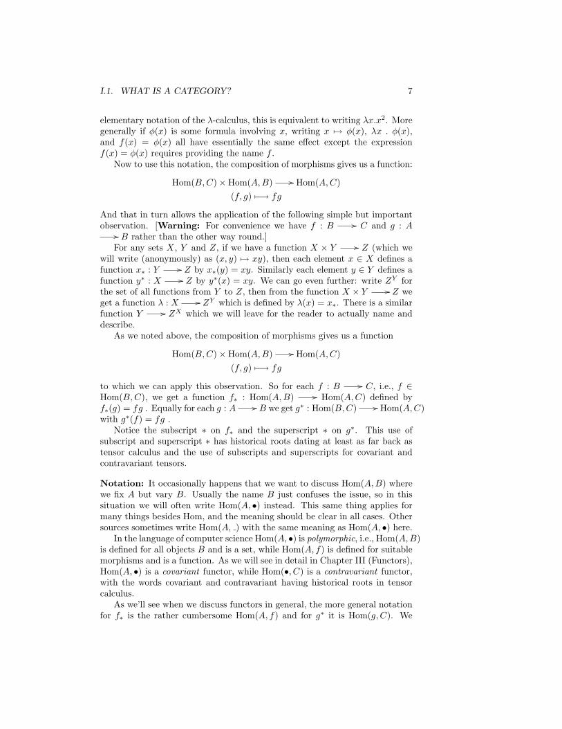
Now to use this notation, the composition of morphisms gives us a function:
Hom(B,C)×Hom(A,B) // Hom(A,C)(f, g) 7−→ fg
And that in turn allows the application of the following simple but importantobservation. [Warning: For convenience we have f : B // C and g : A
// B rather than the other way round.]For any sets X, Y and Z, if we have a function X × Y // Z (which we
will write (anonymously) as (x, y) 7→ xy), then each element x ∈ X defines afunction x∗ : Y // Z by x∗(y) = xy. Similarly each element y ∈ Y defines afunction y∗ : X // Z by y∗(x) = xy. We can go even further: write ZY forthe set of all functions from Y to Z, then from the function X × Y // Z weget a function λ : X // ZY which is defined by λ(x) = x∗. There is a similarfunction Y // ZX which we will leave for the reader to actually name anddescribe.
As we noted above, the composition of morphisms gives us a function
Hom(B,C)×Hom(A,B) // Hom(A,C)(f, g) 7−→ fg
to which we can apply this observation. So for each f : B // C, i.e., f ∈Hom(B,C), we get a function f∗ : Hom(A,B) // Hom(A,C) defined byf∗(g) = fg . Equally for each g : A // B we get g∗ : Hom(B,C) // Hom(A,C)with g∗(f) = fg .
Notice the subscript ∗ on f∗ and the superscript ∗ on g∗. This use ofsubscript and superscript ∗ has historical roots dating at least as far back astensor calculus and the use of subscripts and superscripts for covariant andcontravariant tensors.
Notation: It occasionally happens that we want to discuss Hom(A,B) wherewe fix A but vary B. Usually the name B just confuses the issue, so in thissituation we will often write Hom(A, •) instead. This same thing applies formany things besides Hom, and the meaning should be clear in all cases. Othersources sometimes write Hom(A, ) with the same meaning as Hom(A, •) here.
In the language of computer science Hom(A, •) is polymorphic, i.e., Hom(A,B)is defined for all objects B and is a set, while Hom(A, f) is defined for suitablemorphisms and is a function. As we will see in detail in Chapter III (Functors),Hom(A, •) is a covariant functor, while Hom(•, C) is a contravariant functor,with the words covariant and contravariant having historical roots in tensorcalculus.
As we’ll see when we discuss functors in general, the more general notationfor f∗ is the rather cumbersome Hom(A, f) and for g∗ it is Hom(g, C). We

8 CHAPTER I. MATHEMATICS IN CATEGORIES
will commonly use f∗ and g∗, but sometimes fA∗ if we need to keep trackof the object A and sometimes the full Hom(A, f) or even C (A, f) if all theinformation is needed. Similarly we will usually write g∗, but sometimes g∗C ,Hom(g, C) or C (g, C).
We sometimes want to describe the functions f∗, and g∗ without using thenotation or even necessarily mentioning f or g specifically, so then we will writeof “the induced functions” on the Hom sets.
For the record, here are the formal definitions.
Definition I.7: For each morphism f : B // C, the formula f∗(g) = fgdefines the induced function f∗ : Hom(A,B) // Hom(A,C).
Definition I.8: For each morphism g : A // B, the formula g∗(f) = fgdefines the induced function g∗ : Hom(B,C) // Hom(A,C).
When we come to discuss functors in Chapter III (Functors), these willbe primary examples. In that context we want to note a few simple facts thatwe will use often: (fg)∗ = f∗g∗ and (fg)∗ = g∗f∗; (1B)∗ = Hom(A, 1B) =1Hom(A,B) and (1A)∗ = Hom(1A, B) = 1Hom(A,B).
We also want to note another connection between categories and monoids.If C is any category and C is any object in C , then C (C,C) is a monoid withcomposition as the binary operation and 1C as the identity.
This is sufficiently important that we have a couple of definitions.
Definition I.9: In any category, a morphism in which the domain and codomainare equal is called an endomorphism.
Definition I.10: When C is an object of C as above, C (C,C) is the monoidof endomorphisms, or the endomorphism monoid, of C.
I.1.2 Subcategories
The most convenient source of additional categories is through the notion of asubcategory.
Definition I.11: A category S is a subcategory of category C provided:
1. Every object of S is an object of C .
2. If f ∈ S (A,B), then f ∈ C (A,B).
3. If f : A // B and g : B // C in S , then gf is also the compositionof g following f in C .
4. If 1A is the identity morphism for A in S , then 1A is also the identitymorphism for A in C .

I.1. WHAT IS A CATEGORY? 9
Examples of subcategories abound. A few of the examples that are discussedin the Catalog of Categories (Appendix B) are: The category of finite sets,FiniteSet, cf. Section B.1.2, as a subcategory of the category of sets; thecategory of Abelian groups, Ab cf. Section B.2.7, as a subcategory of thecategory of groups, Group (cf. Section B.2.5;) the category of lattices, Latticecf. Section B.6.3, as a subcategory of the category of partially ordered sets,Poset cf. Section B.6.2; the category of compact Hausdorff spaces, Comp cf.Section B.9.4, as a subcategory of the category of topological spaces, Top cf.Section B.9.3; and the category of Hilbert spaces, Hilbert cf. Section B.13.4,as a subcategory of the category of Banach spaces, cf. Section B.13.1.
In addition the notion of subcategory generalizes the notion of submonoid,subgroup, etc. For if S is a submonoid of the monoid M , then, considered ascategories, S is a subcategory of the category M , etc.
For the moment our interest in subcategories will be entirely as a wayof specifying additional categories. To date all we have mentioned are justgotten specifying some collection of objects in the containing category. Thatis sufficiently common and important that we record it as:
Definition I.12: A subcategory S of C is full when for all objects A and Bof S we have S (A,B) = C (A,B).
Of course subcategories need not be full subcategories. As an example,starting with the category of sets we define a new category Iso(Set) with thesame objects, i.e., sets, but as morphisms only the bijections. As every identityfunction is a bijections and the composition of bijections is a bijection, Iso(Set)is clearly a subcategory of Set. Not every function is a bijection, so Iso(Set)is not a full subcategory. The notation Iso(Set) may appear odd, but this ispart of a general situation as we will see in Section I.2.1 (see page 11.)
I.1.3 Recognizing Categories
To practice recognizing categories, we start with some very small and somewhatartificial examples.
The empty category 0 is the category with no objects and no morphisms.All the requirements in the definition of a category are vacuously satisfied. Itis interesting and useful in much the same way the empty set is useful.
The one element category 1 is an essentially unique category with one objectand one morphism which must be the identity morphism on the one object.
The category we call 2 or the arrow category is illustrated by the followingdiagram.
0$$ ! // 1 dd
where all of the arrows represent distinct morphisms, and there are noother morphisms. For this to be a category, the two circular arrows must bethe identity morphisms, and that completely determines composition, which iseasily seen to be associative.

10 CHAPTER I. MATHEMATICS IN CATEGORIES
Next consider the following diagram:
∗
???????
0$$
??// 1 dd
with each node representing an object and each arrow representing a distinctmorphism.
Exercise I.1. Verify that there is a unique fashion in which this is a categorywith three objects and six morphisms. This category is named 3.
Although these examples may seem strange they will actually recur in var-ious application later in these notes.
As the last little example look at the following diagram:
0$$
1 dd0 1
0 1oo0 1??
Exercise I.2. If each arrow in the above diagram represents a distinct mor-phism, can this be a category with two objects and five morphisms?
In the previous section we saw the example of Iso(Set) as a somewhatunusual category. Let’s look at a few more.
Define a subcategory M of Set to have as objects all sets, but the only mor-phisms are the injective functions, i.e., f : X // Y where f(x1) = f(x2) ⇒x1 = x2. Clearly the identity function on any set is in M , and the composi-tion of any two injective functions is again injective, so we see M is indeed asubcategory, but not a full subcategory, of Set.
Exercise I.3. Define a subcategory E of Set to have as objects all sets, but theonly morphisms are the surjective functions, i.e., f : X // Y where for everyy ∈ Y there exists some x ∈ X with f(x) = y. Verify that E is a subcategory,but not a full subcategory, of Set.
I.2 Special Morphisms
CONVENTION: In this section all the objects and morphisms are inthe one fixed category C Unless explicitly mentioned to the contrary.
I.2. SPECIAL MORPHISMS 11
I.2.1 Isomorphisms
Besides the identity morphisms that exist in every category, there are othermorphisms that are important and interesting parts of mathematics in a cate-gory. The first are isomorphisms.
Definition I.13: An isomorphism, f : A // B, is a morphism with aninverse, f−1 : B // A, satisfying f−1f = 1A and ff−1 = 1B .
Note that if f has an inverse, then it is unique, justifying the notation f−1.To see the uniqueness note that if g and h are both inverses, then g = 1Ag =hfg = h1B = h.
Notation: As is often done in algebra, we will use the symbol ∼= to indicate
an isomorphism. So we will write f : A∼= // B to indicate that f is an
isomorphism, and we will write A ∼= B and say “A is isomorphic to B” whenthere is an isomorphism from A to B.
Just a bit earlier we introduced the endomorphism monoid of an object.Now in any monoid M with identity element 1, there is the submonoid ofinvertible elements: G = m ∈ M | ∃m−1 such that mm−1 = 1 = m−1m.As every element of G has an inverse, G is actually a group called, unoriginally,the group of invertible elements of M .
Applying this to the monoid of endomorphisms of any object in a cate-gory, we get the group of automorphisms or automorphism group of theobject.
Here are the formal definitions.
Definition I.14: An automorphism is an endomorphism that is also anisomorphism.
Definition I.15: The automorphism group of an object C is the group ofall automorphisms of C. This is usually denoted by Aut(C).
So Aut(C) is the group of invertible elements of the monoid of endomor-phisms of C. In particular the identity morphism for any object C is an auto-morphism of C and is the identity in the group Aut(C).
Back in Section I.1.2 we met Iso(Set), a subcategory of the categories ofsets that is not a full subcategory. As mentioned there this is an example ofa general construction. For any category C there is the subcategory Iso(C )of C which has the same objects, but with the morphisms of Iso(C ) beingthe isomorphisms of C (and that is the origin of the notation.) This is a fullsubcategory of C only when every morphism of C is an isomorphism (and then,of course, the two categories are the same.)
Categories such as this are actually of sufficient interest to deserve specialstudy in their own right – for example see Higgins [32]. As a start we note thefollowing definition.

12 CHAPTER I. MATHEMATICS IN CATEGORIES
Definition I.16: A groupoid is a category in which every morphism is anisomorphism.
Now just as a monoid is a category with just one object, a group is agroupoid with just one object. More information, including examples andapplications, are in Appendix B.18 (Catalog of Categories).
A frequently useful technique in category theory is to connect properties ofmorphisms with properties of the functions they induce on Hom sets. Isomor-phisms provide our first example in the next two exercises.
Exercise I.4. For any category C , prove that if f : A // B is an isomor-phism, then for every object C the functions
fC∗ : Hom(C,A) // Hom(C,B) and f∗C : Hom(B,C) // Hom(A,C)
are isomorphisms (i.e., bijections) as well.
Exercise I.5. Suppose f : A // B is a morphism where for every object Cthe functions
fC∗ : Hom(C,A) // Hom(C,B) and f∗C : Hom(B,C) // Hom(A,C)
are bijections. Prove that f is an isomorphism.
Exercise I.6. Suppose that f : A // B is an isomorphism in C . Define afunction C (A,A) // C (B,B) by e ∈ C (A,A) 7→ fef−1 ∈ C (B,B). Showthat this function is a monoid homomorphism, and indeed an isomorphism.
In general an isomorphism of monoids is easily seen to also give rise to anisomorphism of the group of invertible elements in the monoids, so in particularwhenever f : A // B is an isomorphism the function defined above also givesan isomorphism between Aut(A) and Aut(B).
I.2.2 Sections and Retracts
The definition of an isomorphism has two parts which are really separable, andthat leads to the notions of sections and retracts which we define here.
Definition I.17: For any morphism f : A // B, a section of f is a mor-phism s : B // A such that fs = 1B .
Definition I.18: For any morphism f : A // B, a retract (or retract) off is a morphism r : B // A such that rf = 1A.

I.2. SPECIAL MORPHISMS 13
A section is also called a right inverse,while a retract is alternatively calleda left inverse.
Exercise I.7. Consider any morphism f . Verify the following:
1. f has a section iff f∗ always has a section.
2. f has a retract iff f∗ always has a section.
3. f has a retract implies f∗ always has a retract.
4. f has a section implies f∗ always has a retract.
It is a trivial observation that s is a section for r iff r is a retract for s.Note the usage of “iff”as an abbreviation for “if and only if”. As noted in
the preface (p. iv) we will use that from time to time throughout these notes.It is not an accident that we have iff in the first two parts of this exercise,
but only implication in the last two. Can you find examples where f∗ has aretract, but f does not? What about where f∗ has a retract but f does nothave a section? [Warning : You won’t find such examples in the category ofsets.] We will return to this in exercises I.12 and I.18.
Exercise I.8. Clearly if f is an isomorphism, then f−1 is both a section anda retract for f . Show that if s is a section for f and r is a retract for f , thenr = s and so f is an isomorphism.
Exercise I.9. In the category of sets, give examples of functions that have asection but not a retract, and that have a retract but not a section. Also giveexamples of functions that have neither a section nor a retract.
I.2.3 Epimorphisms and Monomorphisms
In the category of Sets, the categorical notions of having a section or havinga retract capture the essence of surjections and injections without any explicitmention of the elements of the sets. But these notions do not work nearly sowell in other categories.
As one simple example consider the homomorphism q : Z // Z2 (in thecategory of Abelian groups)defined by q(n) = n mod 2 (Z being the group ofintegers, and Z2 the group of integers modulo 2.) Now q is a surjection, but itcertainly does not have a section - indeed the only homomorphism of Z2 to Ztakes both elements of Z2 to 0. [For more information see the section on thecategory of groups see Section B.2.7 of the Catalog of Categories. The generalreference for information about Abelian groups, and other general topics inabstract algebra, is Mac Lane and Birkhoff’s Algebra [55].]

14 CHAPTER I. MATHEMATICS IN CATEGORIES
Fortunately there is a weaker property than having a right inverse, thatcaptures the notion of a surjection in a categorical fashion for a great manycategories. Moreover it turns out to be important and useful quite generally.Note that in many “algebraic” categories such as the categories of groups,Abelian groups, rings, etc, a surjective homomorphism is usually called anepimorphism, and that is the name used throughout these notes.
Definition I.19: In any category, a morphism e : A // B is an epimor-phism iff fe = ge implies f = g.
The equation fe = ge means that f and g are two morphisms with domainB and the same codomain. The codomain wasn’t explicitly mentioned becauseit’s name is irrelevant.
Note: As is common in mathematical writing, there is an implicit universalquantifier in the definition of an epimorphism. We have an epimorphism e onlyif for all morphisms f and g, ef = eg implies e=f. Even one exception and eis not an epimorphism.
This is called a cancellation law, and we say that e is an epimorphism iff itcan be canceled on the right or has right cancellation. That “right cancellation”is a weakened form of “having a right inverse” is the content of this nextexercise.
Exercise I.10. Prove that if a morphism f has a section, then f is an epi-morphism.
This result can be restated as “every retract is an epimorphism” whichpartly explains why retracts are also called split epimorphisms .
Notation: We often use the special arrow // // to indicate an epimorphism.When writing about epimorphisms, other words are sometimes used – we
sometimes use the abbreviated form epi , and epic, particularly as an adjective(“the map f is epic”.)
As with sections and retracts, let’s also connect this with the Hom sets.
Exercise I.11. Show that f : A // B is an epimorphism iff for every objectC, the functions f∗C are all injective.
Exercise I.12. Find an example where f : A // B is an epimorphism, butfor some object C the function fC∗ is not surjective. [Warning: You need touse something other than the category of sets.]
The next three exercises ask you to work out the meaning of epimorphismsin a few special cases where the categories are monoids.
There are two familiar binary operation on the set of natural numbers,

I.2. SPECIAL MORPHISMS 15
addition and multiplication. Each of them gives us a monoid. The first iscalled the additive monoid of natural numbers, while the second is called themultiplicative monoid of natural numbers.
Exercise I.13. Consider N, the monoid of natural numbers with the binaryoperation of addition as a category with one object. Show that every morphismin Nis an epimorphism.
The next exercise asks you to consider epimorphisms in a more complicatedmonoid.
Let A = a, b be a set with two elements. Define A∗ to be the set of allfinite sequences from A, i.e.,
A∗ = (), (a), (b), (a, a), (a, b), (b, a), (b, b), (a, a, a), · · · .
Define a binary operation onA∗ to be concatenation, i.e., if s = (s1, s2, · · · , sm)and t = (t1, t2, · · · , tn) are in A∗, then st = (s1, s2, · · · , sm, t1, t2, · · · , tn). Thismakes A∗ into a monoid with (), the empty sequence as the identity. [This isthe free monoid on A and is one example of many “free” structures that willbe discussed in these notes. More information on free monoids can be found inSections B.19.3 and III.2.12, and in Bourbaki’s Algebra (Part I) [10, I, §7].]
We will usually write just a or b rather than (a) and (b). And with that no-tation (s1s2 · · · sm) = s1s2 · · · sm and we can think of that as either the productof the elements s1, s2, . . ., or as composition of the morphisms s1, s2, . . ..
[In mathematical logic and theoretical computer science the monoid A∗ iscalled the Kleene closure of A after the logician Stephen Kleene who used itin his study of regular expressions. The construction actually make sense forsets with any number of elements, and this is the more general context of theKleene closure.]
Exercise I.14. Show that every morphism in A∗ is an epimorphism.
And finally we look at a monoid where not every morphism is an epimor-phism.
Let R be the compatible equivalence relation on A∗ generated by a2, ab,and consider the quotient monoid B = A∗/R. This means that in B we havea2 = ab, a2b = ab2 = a3, and all other relations that follow from a2 = ab. Bycontrast ba is not equal to anything else.
[More information about generated equivalence relations and the associatedquotients can be found in the Appendix on Set Theory (see Section A.7), andin the material on the categories Monoid and Semigroup in the Catalog ofCategories (see Sections B.2.3 and B.2.2.) There is also a detailed treatmentin Bourbaki [10, I, §1.6].]
In B every element has a unique canonical form that is one of am, bn, orbnam. There is nothing more complicated because any element of the form

16 CHAPTER I. MATHEMATICS IN CATEGORIES
ambn = am+n and that in turn will simplify any expression that has an ab init somewhere.
Exercise I.15. Using the above show that b is an epimorphism in B consideredas a monoid with one object, but a is not an epimorphism.
Now the term epimorphism already has a meaning in a number of familiarcategories, so we would certainly like to know that the new definition we havejust given is actually the same as the usual one. In just a moment we’ll see thisis indeed true in some important examples, but there are other cases where it isnot at all easy to verify this and many more where it is false. More informationon this topic for the specific categories discussed can be found in the Catalogof Categories in Appendix B.
In the category Ab of Abelian groups and group homomorphisms (see Sec-tion B.2.7,) it is easy to see that every epimorphism in the usual sense, i.e., asurjective group homomorphism, is an epimorphism in the the sense of defi-nition I.19. Just note that if e is a surjective homomorphism and fe = ge,then for each b ∈ B there is some a ∈ A so that b = e(a). But thenf(b) = f(e(a)) = g(e(a)) = g(b), and so f = g.
The converse uses some more information about Abelian groups. Recallthat for any homomorphism f : A // B of Abelian groups the image of f ,Im(f) = f(a)|a ∈ A is a (normal) subgroup and there is a quotient groupB/Im(f) and a quotient map q : B // B/Im(f).
Now suppose that e : A // B has the cancellation property that is thedefinition of an epimorphism in a category, and consider
Ae // B
0 //q
// B/Im(e)
where q is the quotient map, and 0 maps every element to the zero element.Surely 0e = 0, but also qe = 0. So q = 0! But that says B/Im(e) is the zerogroup, i.e., that B = Im(e) and e is surjective.
Very much the same thing is true in the category Vect of vector spaces andlinear transformations (see Section B.4.3.) Every surjective linear transforma-tion is an epimorphism as defined above with exactly the same argument asabove.
The proof of the converse is much the same as well. Every linear trans-formation f : A // B has an image Im(f) = f(a)|a ∈ A which is asubspace of B, and there is a quotient space B/Im(f) and a quotient mapq : B // B/Im(f). Just as with Abelian groups, if e : A // B has rightcancellation, then consider
Ae // B
0 //q
// B/Im(e)
where q is the quotient map, and 0 maps every element to the zero element.Surely 0e = 0, but also qe = 0. So q = 0! But that says B/Im(e) is the zerovector space which only happens when B = Im(e), so e is surjective.

I.2. SPECIAL MORPHISMS 17
In Chapter XIII we’ll see that there are a large variety of additional cate-gories where very similar arguments apply.
By contrast, proving that a homomorphism in the category of groups (i.e., notnecessarily Abelian) which has the epimorphism cancellation property is actu-ally surjective is not nearly so easy. See section B.2.5 on page 227 for moredetail.
Just as “having a right inverse” can be weakened to “right cancellation”,“having a left inverse” can be weakened to “left cancellation”.
Definition I.20: In any category, a morphism m : A // B is a monomor-phism iff mf = mg implies f = g.
This is another “cancellation law”,so we say that m is a monomorphism iffit can be canceled on the left or has left cancellation.
That “left cancellation” is a weakened form of “having a left inverse” is thecontent of this next exercise.
Exercise I.16. Prove that if a morphism f has a retract, then f is a monomor-phism.
This result can be restated as “every section is a monomorphism” whichpartly explains why sections are also called split monomorphisms .
Just as with epimorphisms, other words are sometimes used – we sometimessay a morphism is monic or mono or is a monic.
Notation: We use the special arrow // // to indicate a monomorphism.Again let’s connect this with the Hom sets.
Exercise I.17. Show that f : A // B is a monomorphism iff for all objectsC the functions fC∗ are always injective.
Exercise I.18. Find an example where f : A // B is an monomorphism,but for some object C the function f∗C is not surjective. [Warning: You needto use something other than the category of sets.]
Just as with epimorphism, monomorphism already has a meaning in a num-ber of familiar categories and we would certainly like to know that the newdefinition we have just given is actually the same as the usual one. In just amoment we’ll see this is indeed true in some important examples, but thereare other cases where it is not at all easy to verify this. More information onthis topic for the specific categories discussed can be found in the Catalog ofCategories in Appendix B.
In the category Ab of Abelian groups and group homomorphism, it is easyto see that every monomorphism in the usual sense, i.e., a group homomorphism

18 CHAPTER I. MATHEMATICS IN CATEGORIES
that is injective or one-to-one, is a monomorphism in the the sense of definitionI.20. Just note that if e is an injective homomorphism and mf = mg, then foreach a ∈ A, mf(a) = mg(a) and so f(a) = g(a), i.e., f = g.
The converse uses some more information about Abelian groups. Recallthat for each homomorphism f : A // B of Abelian groups we have thekernel of f , Ker(f) = a ∈ A|f(a) = 0, a subgroup of A with inclusion mapi : Ker(f) // A.
Now suppose that m : A // // B has the left cancellation property that isthe definition of an monomorphism in a category, and consider
Ker(m)0 //i
// Af // B
where i is the inclusion map, and 0 maps every element to the zero element.Now m0 = 0 = mi, so 0 = i! But that says Ker(m) = 0 and so m is injective.
This argument works equally well in the category of groups as in the cate-gory of Abelian groups.
Essentially the same argument works in the category Vect of vector spacesand linear transformation as well. The first part of the argument is exactlythe same, while there is just a small change of terminology in the secondpart. Associated to a linear transformation f : A // B is its null space,N(f) = a ∈ A|f(a) = 0, with inclusion map i : N(f) // A. The rest of theargument is the same: if m : A // // B has left cancellation then consider
Ker(m)0 //i
// Af // B
where i is the inclusion map, and 0 maps every element to the zero element.Now m0 = 0 = mi, so 0 = i! But that says N(m) = 0 and so m is injective.
Before continuing we record as exercises some simple observations that willbe useful as we go along.
Exercise I.19. Show that in any category the composition of retracts is aretract.
Exercise I.20. Show that in any category if gf is a retract, then g is a retract.
Exercise I.21. Show that in any category the composition of epimorphismsis an epimorphism.
Exercise I.22. Show that in any category if gf is an epimorphism, then g isan epimorphism.
I.2. SPECIAL MORPHISMS 19
Exercise I.23. Show that in any category if s is an epimorphism and a section,then s is an isomorphism.
Exercise I.24. Show that in any category the composition of sections is asection.
Exercise I.25. Show that in any category if gf is a section, then f is a section.
Exercise I.26. Show that in any category the composition of monomorphismsis a monomorphism.
Exercise I.27. Show that in any category if gf is an monomorphism, then fis a monomorphism.
Exercise I.28. Show that in any category if r is a monomorphism and aretract, then r is an isomorphism.
In many, though far from all, of the familiar categories discussed in the Cat-alog of Categories (Appendix B) the epimorphisms are the surjective functions,and the monomorphisms are the injective functions. As a result it is often thecase that morphisms that are both monic and epic are isomorphisms. Often,but not always!
Exercise I.29. Give an example of a morphism in a category of “sets withstructure” that is an epimorphism, but not surjective. (Hint: Look in thecategory of monoids or in the category of topological spaces.)
For reasons explained in it is considerably harder to give examples of monomor-phisms which are not injective. The most common example is in the categoryof divisible Abelian groups where the quotient homomorphism Q // Q/Z isa monomorphism but clearly not an injection.
Exercise I.30. Give an example of a category and a morphism in the categorywhich is both a monomorphism and an epimorphism, but not an isomorphism.
This is sufficiently common that it deserves a name.
Definition I.21: A morphism that is both a monomorphism and an epimor-phism is called a bimorphism.

20 CHAPTER I. MATHEMATICS IN CATEGORIES
Of course every isomorphism is a bimorphism, while the last exercises ex-hibits a bimorphism that is not an isomorphism. The interesting question is“When is a bimorphism an isomorphism?”. There are categories where this isalways true, and others where the bimorphisms that are not isomorphisms areof particular interest. This is a minor theme that will recur from time to time.
Again the situation where every bimorphism is an isomorphism has a name.
Definition I.22: A category is which every bimorphism is an isomorphismis called a balanced category.
I.2.4 Subobjects and Quotient Objects
Although “surjective” and “injective” are defined in terms of elements andso don’t quite fit our “arrows only” motto, we will investigate the relationbetween these pairs of concepts (and sections and retracts as well) repeatedly.In particular the relation between these concepts not just in a single category,but between related categories.
As a start notice that in most familiar categories we have notions of sub-objects and quotient objects. These are usually defined in terms of elements,but we’ll do it with morphisms.
Definition I.23: A subobject of an object B is a monomorphism A // // B.
Before continuing on, let’s look at how meaningful this is in the category ofsets. We know that a monomorphism A // // B in Set is an injective function,so certainly if A is a subset of B, then the inclusion function is a monomorphismand so we have a subobject of B. But just because A // // B is an injection,this does not mean that A is a subset of B. But any injection does factor as
A∼= // S → B
with S the image of the monomorphism being an actual subset of B and S → Bthe inclusion function. Moreover two injections m : A // // B and m′ : A′// // B have the same image in B exactly when there is a bijection between A
and A′ so thatA
B
m
???????????A
A′
OO
∼=
A′
B
m′
??
commutes. The same is true in many categories of “structured sets”. Basedon this we make the following definition.

I.2. SPECIAL MORPHISMS 21
Definition I.24: Two subobjects m : A // // B and m′ : A′ // // B of B areequivalent when there is an isomorphism between A and A′ with
A
B
m
???????????A
A′
OO
∼=
A′
B
m′
??
commuting.
So in the category of sets a subset determines a subobject and a subobjectdetermines a subset with two different subobjects determining the same subsetiff they are equivalent. In many other familiar categories such as the cate-gories of groups, rings, vector spaces, etc., there is the same correspondencebetween equivalent subobjects and the familiar subgroups, subrings, etc. But,as just one example, subobjects in the category Top does not well correspondto subspaces of topological spaces. For the details see the various entries in theCatalog of Categories (Appendix B).
It is tempting to define a subobject of an object to be an equivalence class ofequivalent monomorphisms into the object, and it is common to do so. But thedifficulty with this is that such an equivalence class need not exist! In Zermelo-Fraenkel set theory as discussed in Appendix A, the “equivalence class” of allinjections into a one element set, say 0, cannot exist as a set – it is toolarge. Remember that for every set X there is the one element set X andand a unique injection X // // 0. Any two of these are equivalent, so ifthis equivalence class were to exist as a set it would be equinumerous with the(non-existent) set of all sets!
This issue will be dealt in a much more satisfying fashion when we discusssubobject classifiers (see definition IX.1 and the following surrounding mate-rial).
There is the dual notion of a quotient object.
Definition I.25: A quotient object of an object B is an epimorphism
B // // A.
Just as with subobjects we define equivalent quotient objects.
Definition I.26: Two quotient objects e : B // // A and e′ : B // // A′ are
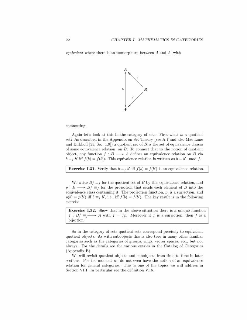
22 CHAPTER I. MATHEMATICS IN CATEGORIES
equivalent where there is an isomorphism between A and A′ with
A
B
____
e
???????????A
A′
OO
∼=
A′
B
e′
commuting.
Again let’s look at this in the category of sets. First what is a quotientset? As described in the Appendix on Set Theory (see A.7 and also Mac Laneand Birkhoff [55, Sec. 1.9]) a quotient set of B is the set of equivalence classesof some equivalence relation on B. To connect that to the notion of quotientobject, any function f : B // A defines an equivalence relation on B viab ≡f b′ iff f(b) = f(b′). This equivalence relation is written as b ≡ b′ mod f .
Exercise I.31. Verify that b ≡f b′ iff f(b) = f(b′) is an equivalence relation.
We write B/ ≡f for the quotient set of B by this equivalence relation, andp : B // B/ ≡f for the projection that sends each element of B into theequivalence class containing it. The projection function, p, is a surjection, andp(b) = p(b′) iff b ≡f b′, i.e., iff f(b) = f(b′). The key result is in the followingexercise.
Exercise I.32. Show that in the above situation there is a unique functionf : B/ ≡f // A with f = fp. Moreover if f is a surjection, then f is abijection.
So in the category of sets quotient sets correspond precisely to equivalentquotient objects. As with subobjects this is also true in many other familiarcategories such as the categories of groups, rings, vector spaces, etc., but notalways. For the details see the various entries in the Catalog of Categories(Appendix B).
We will revisit quotient objects and subobjects from time to time in latersections. For the moment we do not even have the notion of an equivalencerelation for general categories. This is one of the topics we will address inSection VI.1. In particular see the definition VI.6.

I.3. SPECIAL OBJECTS 23
I.3 Special Objects
I.3.1 Products and Sums
Definition I.27: The product of a finite family C1, · · · , Cn of objects inC is an object, P , together with a family of morphisms πi : P // Ci so thatfor every family of morphisms fi : C // Ci there exists a unique morphism〈f1, · · · , fn〉 : C // P with that πi〈f1, · · · , fn〉 = fi.
C P〈f1,··· ,fn〉 //_________C
Ai
fi
''OOOOOOOOOOOOOOOOOOO P
Ai
πi
[We read this diagram as saying that 〈f1, · · · , fn〉 is the unique morphismmaking the diagram commute. Note that implicitly there are n triangles inthis diagram featuring (π1, f1), . . . , (πn, fn) and all with the common edge〈f1, · · · , fn〉.]
Similar situations occur constantly in the study of categories, under thename Universal Mapping Property. The Universal Mapping Property for aproduct ofA1, · · · , An is that every family of morphisms fi : C // Ai uniquelyfactors through the family πi : P // Ai of projections. We will mention ex-amples of other Universal Mapping Properties as they occur, and then discussthe many ramifications in Chapter V (Universal Mapping Properties).
Note: The definition of a product is a template for universal mapping prop-erty definitions throughout category theory, so it is important to understandjust what is required to prove that something is a product.
The important first part is that a product is not just an object. In settheory there is the product of two sets, and it is a certain unique set. Inthe category of sets by contrast, a product of two sets is a set together withtwo projection functions. And while products in the category of sets are in aimportant certain sense unique (see the next proposition), it is definitely notthe object that is unique.
The next crucial part of the definition is the requirement that for everyobject C in the category, and for every family of morphisms fi : C // Ai amorphism f : C // P exists such that for all i we have πif = fi.
And the final critical requirement is that the morphism f which is assertedto exist in the previous paragraph is the unique morphism which satisfies thoseequations, i.e., if we have both f and g with πif = fi = πig, then it must followthat f = g.
And equally, these are exactly the properties that can be used when wehave the hypothesis that (P, πi : P // Ai) is a product of the family (Ai) ofobjects.
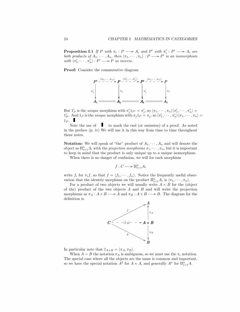
24 CHAPTER I. MATHEMATICS IN CATEGORIES
Proposition I.1 If P with πi : P // Ai and P ′ with π′i : P ′ // Ai areboth products of A1, · · · , An, then 〈π1, · · · , πn〉 : P // P ′ is an isomorphismwith 〈π′1, · · · , π′n〉 : P ′ // P as inverse.
Proof: Consider the commutative diagram
Ai Ai
P ′
Ai
π′j
P ′ P〈π1,··· ,πn〉 //_____ P
Ai
πj
Ai Ai
P
Ai
P P ′〈π′1,··· ,π
′n〉 //_____ P ′
Ai
π′j
Ai Ai
P ′
Ai
P ′ P〈π1,··· ,πn〉 //_____ P
Ai
πj
But 1′P is the unique morphism with π′j1P ′ = π′j , so 〈π1, · · · , πn〉〈π′1, · · · , π′n〉 =1′P . And 1P is the unique morphism with πj1P = πj , so 〈π′1, · · · , π′n〉〈π1, · · · , πn〉 =1P .
Note the use of to mark the end (or omission) of a proof. As notedin the preface (p. iv) We will use it in this way from time to time throughoutthese notes.
Notation: We will speak of “the” product of A1, · · · , An and will denote theobject as Πn
i=1Ai with the projection morphisms π1, · · · , πn, but it is importantto keep in mind that the product is only unique up to a unique isomorphism.
When there is no danger of confusion, we will for each morphism
f : C // Πni=1Ai
write fi for πif , so that f = 〈f1, · · · , fn〉. Notice the frequently useful obser-vation that the identity morphism on the product Πn
i=1Ai is 〈π1, · · · , πn〉.For a product of two objects we will usually write A × B for the (object
of the) product of the two objects A and B and will write the projectionmorphisms as πA : A×B // A and πB : A×B // B. The diagram for thedefinition is
A×B
B
πB
C A×B〈f,g〉___ //___C
B
g
''OOOOOOOOOOOOOOOOOOOO
A
C
77
f
oooooooooooooooooooo A
A×B
OO
πA
In particular note that 1A×B = 〈πA, πB〉.When A = B the notation πA is ambiguous, so we must use the πi notation.
The special case where all the objects are the same is common and important,so we have the special notation A2 for A×A, and generally An for Πn
i=1A.

I.3. SPECIAL OBJECTS 25
The Catalog of Categories (Appendix B) discusses products for all of thecategories there, but it seems worthwhile to at least note the situation in a fewfamiliar categories. In Set, A × B = (a, b)|a ∈ A, b ∈ B with πA(a, b) = aand πB(a, b) = b. And given functions f : C // A and g : C // B,〈f, g〉(c) = (f(c), g(c))
For most of the familiar categories of “structured sets”, e.g., categories ofgroups, rings, vector spaces, topological spaces, etc., the same constructionworks equally well.
Recalling that Hom(C,A)stands for the collection of morphisms from C toA, we can also state the definition as: (Πn
i=1Ai, π1, · · · , πn) is a product iff
Hom(C,Πni=1Ai) // Πn
i=1Hom(C,Ai)f 7−→ (π1f, · · · , πnf)
is a bijection with inverse
Πni=1Hom(C,Ai) // Hom(C,Πn
i=1Ai)(f1, · · · , fn) 7−→ 〈f1, · · · , fn〉
Yet another way of saying this is that for every object C, the morphism〈π1∗, · · · , πn∗〉 : Hom(C,Πn
i=1Ai) // Πni=1Hom(C,Ai) is an isomorphism in
the category of sets.Note that (f1, · · · , fn) is an n-tuple of morphisms, while 〈f1, · · · , fn〉 is
just one morphism, the single unique morphism with πi〈f1, · · · , fn〉 = fi fori = 1, · · · , n.
Now we want to look at an unfamiliar category to illustrate just what isinvolved in showing we do or do not have a product.
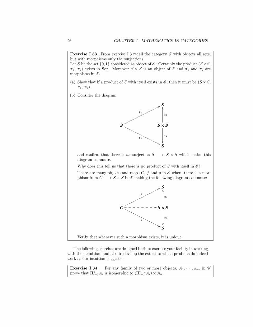
26 CHAPTER I. MATHEMATICS IN CATEGORIES
Exercise I.33. From exercise I.3 recall the category E with objects all sets,but with morphisms only the surjections.Let S be the set 0, 1 considered as object of E . Certainly the product (S×S,π1, π2) exists in Set. Moreover S × S is an object of E and π1 and π2 aremorphisms in E .
(a) Show that if a product of S with itself exists in E , then it must be (S×S,π1, π2).
(b) Consider the diagram
S × S
S
π2
S S × SS S × SS
S
1S
''OOOOOOOOOOOOOOOOOOOO
S
S
77
1S
oooooooooooooooooooo S
S × S
OO
π1
and confirm that there is no surjection S // S × S which makes thisdiagram commute.
Why does this tell us that there is no product of S with itself in E ?
There are many objects and maps C, f and g in E where there is a mor-phism from C // S × S in E making the following diagram commute:
S × S
S
π2
C S × S//________C
S
g
''OOOOOOOOOOOOOOOOOOOO
S
C
77
f
oooooooooooooooooooo S
S × S
OO
π1
Verify that whenever such a morphism exists, it is unique.
The following exercises are designed both to exercise your facility in workingwith the definition, and also to develop the extent to which products do indeedwork as our intuition suggests.
Exercise I.34. For any family of two or more objects, A1, · · · , An, in Cprove that Πn
i=1Ai is isomorphic to (Πn−1i=1 Ai)×An.

I.3. SPECIAL OBJECTS 27
Exercise I.35. Suppose f : P // A × Bis an isomorphism. Prove that(P, π1f, π2f) is also a product of A and B.
Exercise I.36. Define t : A×B // B×Aby t1 = π2, t2 = π1, i.e., t = 〈π2, π1〉.Prove that t is an isomorphism.
The morphism t of the above exercise will be used from time to time, usuallyin connection with commutative operations of some sort. Because of that wewant the following definition.
Definition I.28: The morphism t as defined in exercise I.36 is the transpo-sition isomorphism.
This exercise and definition is a special case of a more general one which isharder only because of the bookkeeping involved in dealing with the indices.
Exercise I.37. With n a positive integer, let p : 1, · · · , n∼= // 1, · · · , n
be a permutation. Define s : Πni=1Ai
// Πni=1Ap(i) by sp(i) = πi. Show that
s is an isomorphism with s−1 : Πni=1Ap(i)
// Πni=1Ai defined by s−1
i = πi
These two exercises are interesting, but can also be misleading. Notice thatthe first exercise does not say that B × A is a productof A and B. Indeed itcannot be overemphasized that a product of two objects is not just an object,but rather an object together with two projection morphisms satisfying theUniversal Mapping Property for a product. The object that is part of theproduct (B × A, πB , πA) is isomorphic to the object A × B and so, followingexercise I.35, there are suitable projections morphisms from B × A to A andB that will give a product. But those projections are not the projections thatare part of (B ×A, πB , πA), even in the special case when A = B!
In many of the familiar categories the projection morphisms from a productto each of its factors is surjective. That suggests that perhaps in categories theyare always surjective, so we ask the following question.
Exercise I.38. Does the projection π1 : A × B // A have to be an epi-morphism? Prove or give a counter-example. (Hint: Carefully consider thecategory of sets.)
There are many familiar constructions for sets that carry over quite readilyto products in arbitrary categories. We start with the following definition.
Definition I.29: Whenever we have fi : Ai // Bi, we define the product of
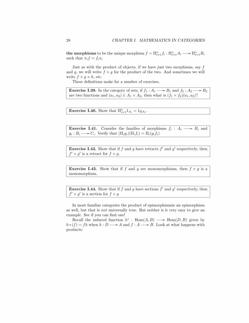
28 CHAPTER I. MATHEMATICS IN CATEGORIES
the morphisms to be the unique morphism f = Πni=1fi : Πn
i=1Ai// Πni=1Bi
such that πif = fiπi
Just as with the product of objects, if we have just two morphisms, say fand g, we will write f × g for the product of the two. And sometimes we willwrite f × g × h, etc.
These definitions make for a number of exercises.
Exercise I.39. In the category of sets, if f1 : A1// B1 and f2 : A2
// B2
are two functions and (a1, a2) ∈ A1 ×A2, then what is (f1 × f2)(a1, a2)?
Exercise I.40. Show that Πni=11Ai = 1ΠAi .
Exercise I.41. Consider the families of morphisms fi : Ai // Bi andgi : Bi // Ci. Verify that (Πigi)(Πifi) = Πi(gifi)
Exercise I.42. Show that if f and g have retracts f ′ and g′ respectively, thenf ′ × g′ is a retract for f × g.
Exercise I.43. Show that if f and g are monomorphisms, then f × g is amonomorphism.
Exercise I.44. Show that if f and g have sections f ′ and g′ respectively, thenf ′ × g′ is a section for f × g
In most familiar categories the product of epimorphismsis an epimorphismas well, but that is not universally true. But neither is it very easy to give anexample. See if you can find one!
Recall the induced function h∗ : Hom(A,B) // Hom(D,B) given byh∗ (f) = fh when h : D // A and f : A // B. Look at what happens withproducts:

I.3. SPECIAL OBJECTS 29
Exercise I.45. Suppose that f : A // B, g : A // C and h : D // A.Verify that 〈f, g〉h = 〈fh, gh〉.Hint: Here is the relevant diagram.
D
B
fh
77ooooooooooooooooooooA
B
f
??B × C
B
πB
OO
D Ah // A B × C
〈f,g〉 //A
C
g
??????????? B × C
C
πC
D
C
gh
''OOOOOOOOOOOOOOOOOOOO
Here is a simple but important example which is worthy of a formal defini-tion.
Definition I.30: For every object A this is the diagonal morphism ∆ =〈1A, 1A〉 : A // A×A.
This will be written as ∆A if we need to emphasize the particular object.
Exercise I.46. Verify that for any morphisms f, g : A // B, we have〈f, g〉 = (f × g)∆.
Exercise I.47. Let X be any object of Set. What is ∆(x) for x ∈ X?
Exercise I.48. Let A be any Abelian group in Ab. What is ∆(a) for anya ∈ A?
The answers for the two previous exercises are the same, and for generalreasons we will explain when we discuss Algebraic Categories in Chapter VII.
For every concept defined in a general category, there is a dual concept thatis gotten by “reversing all the arrows”. This notion of duality is itself a verygeneral and important concept that will be discussed at length in Section II.1.Leading up to that we will give many example of dual definitions, theoremsand proofs, starting with the dual of products.
Definition I.31: For any finite family A1, · · · , An of objects in C , a coprod-uct or sum of these objects is an object, S together with a family of morphismιj : Aj // S where for every family of morphisms fj : Aj // C there exists

30 CHAPTER I. MATHEMATICS IN CATEGORIES
a unique morphism f1
...fn
: S // C
such that f1
...fn
ιj = fj
C Soo
0BBBB@f1
...fn
1CCCCA_________C
Ai
gg
fi
OOOOOOOOOOOOOOOOOOO S
Ai
OO
ιi
[We read this diagram as saying that
f1
...fn
is the unique morphism that makes the diagram commute. Note that implicitlythere are n triangles in this diagram featuring (ι1, f1), . . . , (ιn, fn) and all with
the common edge
f1
...fn
.]
Note: In Section I.3.3 we’ll see the good reasons why we would like to writethe morphism from a sum into another object as a column vector, but spaceconsiderations demands a more compact notation, so we will use [f1, · · · , fn]as a synonym for f1
...fn
For reasons that we will explore more fully when we discuss dual cate-
gories and duality in Section II.1, for each result about products, there is acorresponding result about sums. All of the following results in this section,including the exercises, are examples.
Proposition I.2 If S with ιj : Ai // S and S′ with ι′j : Ai // S′ areboth sums of A1, · · · , An, then [ι1, · · · , ιn] : S′ // S is an isomorphism with[ι′1, · · · , ι′n] : S // S′ as inverse.

I.3. SPECIAL OBJECTS 31
Proof: Consider the commutative diagram
S′ S0BBBB@ι1...ιn
1CCCCA
//_____
Ai
S′
ι′j
Ai AiAi
S
ιj
S S′0BBBB@
ι′1...ι′n
1CCCCA
//_____
Ai
S
Ai AiAi
S′
ι′j
S′ S0BBBB@
ι1...ιn
1CCCCA
//_____
Ai
S′
Ai AiAi
S
ιj
But 1S′ is the unique morphism with 1S′ι′j = ι′j , so [ι′1, · · · , ι′n][ι1, · · · , ιn] = 1′S .And 1S is the unique morphism with 1Sιj = ιj , so [ι1, · · · , ιn][ι′1, · · · , ι′n] = 1S .
Compare this solution with the proof of Proposition I.1. The two werewritten carefully to make it clear that each can be transformed into the otherby “reversing the arrows” and exchanging sums and products. This is anexample of duality which is discussed formally in Section II.1.
Notation: We will speak of “the” sum or coproduct of A1, · · · , An and willdenote the object as Σni=1Ai with the injection morphisms
ιj : Aj // Σni=1Ai, j = 1, · · · , n,
but it is important to keep in mind that the sum is only unique up to a uniqueisomorphism.
In the special case of two objects A and B we will usually write A+B forthe sum and write ιA : A // A + B, ιB : B // A + B for the injectionmorphisms.
When A = B the notation ιA is ambiguous, so we must use the ιi notation.The special case where all the objects are the same is common and important,so we have the special notation 2 •A for A+A, and generally n •A for Σni=1A.
When there is no danger of confusion, we will for each morphism
f : Σni=1Ai // C
write fi for fιj , so that f = [f1, · · · , fn]. Remember the frequently usefulobservation that the identity morphism on the sum Σni=1Ai is [ι1, · · · , ιn].
The Catalog of Categories (Appendix B) discusses sums for all of the cat-egories there, and for some of them (such as the categories of Abelian groupsand of vector spaces) the sum is a familiar construction. But more commonly,even in the category of sets, sums are not nearly so well known as products.An initial discussion follows on page 34.
Recalling that Hom(A,C)stands for the set of morphisms from A to C, wecan also state the definition as: (Σni=1Ai, ι1, · · · , ιn) is a sum iff
Hom(Σni=1Ai, C) // Πni=1Hom(Ai, C)
f 7−→ (fι1, · · · , fιn)

32 CHAPTER I. MATHEMATICS IN CATEGORIES
is a bijection with inverse
Πni=1Hom(Ai, C) // Hom(Σni=1Ai, C)
(fι1, · · · , fιn) 7−→ [f1, · · · , fn]
Exercise I.49. For any family of two or more objects A1, · · · , An in C provethat Σni=1Ai is isomorphic to (Σn−1
i=1 Ai) +An. (Compare to exercise I.34.)
Exercise I.50. Suppose f : A + B // S is an isomorphism. Prove that〈S, fι1, fι2〉 is also a sum of A and B. (Compare to exercise I.35.)
Exercise I.51. Define t : A+B // B+A by t1 = ι2, t2 = ι1, i.e., t = [ι2, ι1].Prove that t is an isomorphism. (Compare to exercise I.36.)
Definition I.32: Write t for [ι2, ι1] : A+B // B +A. By the immediatelypreceding exercise this is an isomorphism. Just as with the morphism definedin exercise I.36, we call this the transposition isomorphism.
Just as with products, this last exercise (and the next) is interesting, butcan also be misleading. In particular the previous exercises does not say thatB + A is a sumof A and B. Indeed it cannot be overemphasized that a sumof two objects is not just an object, but rather an object together with twoinclusion morphisms satisfying the Universal Mapping Property for a sum. Theobject that is part of the product (B + A, ιB , ιA) is isomorphic to the objectA + B and so, following exercise I.50, there are suitable injection morphismsfrom A and B to B + A that will give a sum. But those injections are notthe injections that are part of (B + A, ιB , ιA), even in the special case whenA = B!
Exercise I.52. With n a positive integer, let p : 1, · · · , n∼= // 1, · · · , n
be a permutation. Define s : Σni=1Ap(i)// Σni=1Ai by sp(i) = ιi. Show that
s is an isomorphism with s−1 : Σni=1Ai// Σni=1Ap(i) defined by si
−1 = ιi.(Compare to exercise I.37.)
Exercise I.53. Does the injection ι1 : A // A + B have to be a monomor-phism? Prove or give a counter-example. (Compare to exercise I.38.)
Definition I.33: Whenever we have fi : Ai // Bi, we define the sum ofthe morphisms f = Σnj=1fj : Σnj=1Aj
// Σnj=1Bj by the fιj = ιjfj

I.3. SPECIAL OBJECTS 33
Just as with the sum of objects, if we have just two morphisms, say f andg, we will write f + g for the sum of the two. And sometimes we will writef + g + h, etc.
And just as for products this makes for a number of exercises.
Exercise I.54. Show that Σni=11Ai = 1ΣAi . (Compare to exercise I.40.)
Exercise I.55. Consider the families of morphisms fi : Ai // Bi and gi : Bi// Ci. Verify that (Σigi)(Σifi) = Σi(gifi). (Compare to exercise I.41.)
Exercise I.56. Show that if f and g have sections f ′ and g′ respectively, thenf ′ + g′ is a section for f + g. (Compare to exercise I.42.)
Exercise I.57. Show that if f and g are epimorphisms, then f + g is anepimorphism. (Compare to exercise I.43.)
Exercise I.58. Show that if f and g have retracts f ′ and g′ respectively, thenf ′ + g′ is a retract for f + g. (Compare to exercise I.44.)
Just as with products of epimorphisms, in most familiar categories the sumof monomorphism is a monomorphism as well, but that is not universally true.(Indeed that follows from the discussion on duality in Section II.1.) But neitheris it very easy to give an example. See if you can find one!
Exercise I.59. Give an example where f and g are monomorphisms, but f+gis not a monomorphism. (Compare with the remark on page 28.)
Recall the induced function h∗ : Hom(B,A) // Hom(B,D) given byh∗(f) = hf when h : A // D and f : B // A. Look at what happens withsums.

34 CHAPTER I. MATHEMATICS IN CATEGORIES
Exercise I.60. Suppose that f : B // A, g : C // A and h : A // D.Verify that h[f, g] = [hf, hg].Hint: Here is the relevant diagram.
B
B + C
ιB
B
A
f
??????????????B
D
hf
''OOOOOOOOOOOOOOOOOOOOOOOO
B + C A[f,g] // A D
h //
C
D
hg
77ooooooooooooooooooooooooC
A
g
??C
B + C
ιC
OO
(Compare to exercise I.45.)
Here is another simple but important example which is worthy of a formaldefinition. This is the dual of the diagonal morphism from page 29.
Definition I.34: For every object A the codiagonal morphism or foldingmorphism is ∇ = [1A, 1A] : A+A // A.
This will be written as ∇A if we need to emphasize the particular object.
Exercise I.61. Verify that for any morphisms f, g : B // A, we have[f, g] = ∇(f + g). (Compare to exercise I.46.)
So we have a number of simple results about sums that are all dual to thecorresponding properties for products, but what categories actually have sums,and what are sums in the categories where they exist? Most of the familiarcategories do have sums, and in many cases these are very well known, but inthe most basic category of sets the sum is unfamiliar.
If X and Y are disjoint sets, i.e., X ∩ Y = ∅ and f : X // Z andg : Y // Z are any two functions, then we can define [f, g] : X ∪ Y // Zby
[f, g](t) =
f(t) if t ∈ Xg(t) if t ∈ Y
Defining ιX : X // X ∪ Y and ιY : Y // X ∪ Y to be the inclusionmaps, it is clear that (X ∪ Y , ιX , ιY ) is a sum of X and Y . If X and Yare not disjoint, there are nonetheless isomorphic sets X ′ and Y ′ which aredisjoint. (One common construction is X ′ = X×0 and Y ′ = Y ×1,) Thenwith ιX and ιY as the compositions of the isomorphisms to X and Y with theinclusions into X ′ ∪ Y ′, we have (X ′ ∪ Y ′, ιX , ιY ) as a sum of X and Y .

I.3. SPECIAL OBJECTS 35
Definition I.35: This above construction defines the disjoint union of twosets.
It should be clear how to extend this to a arbitrary (finite) sums, and wewill leave the details for the reader.
Exercise I.62. If f0 : A0// B0 and f1 : A1
// B1 are two functions, thendescribe (f0 + f1) on the elements of A0 +A1.
The situation in both the category of Abelian groups and in the categoryof vector spaces is very simple. Define (A + B = A × B, ιA(a) = (a, 0),ιB(b) = (0, b)). Now for any two homomorphisms f : A // C and g : B
// C, define [f, g] by [f, g](a, b) = f(a) + g(b).
Exercise I.63. Verify that (A+B, ιA, ιB) is indeed a sum of A and B in Ab.
Exercise I.64. Let A be any Abelian group in Ab. What is ∇(a)for anya ∈ A?
Exercise I.65. If f1 : A1// B1 and f2 : A2
// B2 are two homomor-phisms of Abelian groups, describe (f1 + f2) on the elements of A1 +A2.
Exercise I.66. Verify that (A + B, ιA, ιB) is indeed a sum of A and B inVect.
Exercise I.67. Let A be any vector space in Vect. What is ∇(a)for anya ∈ A?
Exercise I.68. If f1 : A1// B1 and f2 : A2
// B2 are two lineartransformations of vector spaces, describe (f1 +f2) on the elements of A1 +A2.
The same results hold true more generally in the categories of modules overa ring. These are all examples of Abelian categories which are the topic ofChapter XIII. In other well-known categories, such at the category of groups,there are commonly sums, but the construction is less familiar. These arediscussed in the Catalog of Categories (Appendix B).

36 CHAPTER I. MATHEMATICS IN CATEGORIES
I.3.2 Final, Initial and Zero Objects
In the category of sets there are several types of sets that play an importantrole. The first of these are the one element sets!
Definition I.36: An object 1 is a final object or terminal object iff eachobject A has exactly one morphism from A to 1. We will write this as ! : A
// 1 when we need to name the morphism.
Exercise I.69. Prove that any two final objects in C are isomorphic, and theisomorphism is unique.
Notation: We will speak of “the” final object in a category and and will writeit as 1 and will write the unique morphism from any object to 1 as !, but it isimportant to keep in mind that the final object is only unique up to a uniqueisomorphism.
In Set the final objects are all the singletons, i.e., the sets with exactly oneelement. These are useful objects in the category because it means there is abijection between functions f : 1 // A and the elements of A. Inspired bythis (and other examples we will see later) we make the following definition.
Definition I.37: For any category with a final object, a point in an objectA is a morphism 1 // A.
To see some of the value of these definitions, do the following exercise.
Exercise I.70. Show there is a bijection between the points of A × B andpairs (a, b) where a is a point of A and b is a point of B.
Final objects capture some other properties of singletons as well.
Exercise I.71. If 1 is the final object in a category and A is any object in the
category, prove that A oo 1AA
! // 1 exhibits A as the product of 1 and A.So in any category with a final object, 1×A ∼= A.
Exercise I.72. Verify that every point is a monomorphism.
Unfortunately this is not as general as we would like. In the category Ab ofAbelian groups, the final object is the zero group, and for every Abelian groupA there is only one homomorphism from the zero group to any Abelian group.So the set of “points” in an Abelian group has no correspondence with theset of elements of the group. Although the final object in a category is in one

I.3. SPECIAL OBJECTS 37
sense very trivial, it is also another example of a Universal Mapping Property.Even more, as we will see in section V.1, it is the fundamental example of
a Universal Mapping Property. We will also see that how it relates to eachparticular category is important for distinguishing various types of categories.(See Chapter IX.)
Definition I.38: A Cartesian category or category with finite prod-ucts is one with a final object where every finite number of objects C1, . . . ,Cn has a product.
A final object is sensibly considered to be the product of no objects: it hasno projection morphisms (there are no factors on which to project) but thereis the unique morphism from any object to the final object which has suitablecomposition with all of those non-existent projections!
There is a dual notion (in a sense that will be explained in Section II.1)which is also important.
Definition I.39: An object 0 is an initial object iff there is exactly onemorphism from 0 to each object A.
Exercise I.73. Prove that any two initial objects in C are isomorphic, andthe isomorphism is unique. (Compare to exercise I.69.)
In the category of sets there is exactly one initial object, the empty set,and the unique function from the empty set to any set is the empty function.And while functions from a singleton final object to other sets are quite useful,functions from other sets to the empty set are very dull – there aren’t any! Butexercise I.71 does have a suitable dual.
Exercise I.74. If 0 is the initial object in a category and A is any object in
the category, prove that A1A // A oo 1 0 exhibits A as the sum of 0 and A.
So in any category with a initial object, 0+A ∼= A. (Compare to exercise I.71.)
Definition I.40: A co-Cartesian category or category with finite sumsis one with an initial object where every finite collection of objects C1, . . . , Cnhas a sum.
Just as a final object is a product of no factors, an initial object is sensiblyconsidered to be the sum of no objects: it has no injection morphisms (thereis nothing to inject) but there is the unique morphism from the initial objectto any object which composes properly with all of the non-existent injections!
Initial objects are just as trivial and interesting as final objects. They,too, provide another example of a Universal Mapping Property. Indeed inSection V.1.) we will see they are a fundamental example.

38 CHAPTER I. MATHEMATICS IN CATEGORIES
Sometimes initial objects and final objects are the same, and this deservesa special name.
Definition I.41: In a category that has both an initial object, 0, and a finalobject, 1, there is a unique morphism ! : 0 // 1. If this is an isomorphism,then we speak of a zero object and write it as 0.
Of course in a category with a zero object all initial objects, final objectsand zero objects are then uniquely isomorphic.
Definition I.42: If a category has a zero object, then for any objects A and
B we have A ! // 0 ! // B, i.e., there is a unique morphism which “factorsthrough” the zero object. All such morphisms are called zero morphismsand are denoted by 0.
Although the category of sets does not have a zero object, there are verymany familiar categories that do. In the categories of monoids, of groups, ofAbelian groups, of vector spaces, and many others, there is a trivial object thatis the zero object in the category.
There are also interesting and natural categories that have a zero objectbut which are not “algebraic”. One good example is the category of pointedsets.
Definition I.43: A pointed set is a pair, (X,x0), consisting of a non-emptyset, X, together with an element (called the base point,) x0, of X.
Definition I.44: A morphism between pointed sets f : (X,x0) // (Y, y0) isa function f : X // Y with f(x0) = y0.
Just as we have the category Set of sets and functions, we have the categorySet∗ of pointed sets together with their morphisms. For more details see B.1.7.
The category Set∗ has initial objects, final objects and zero objects: any oneelement set with the single element being (necessarily) the base point element.
Set∗ has products and sums. The product of two pointed sets, (X,x0) and(Y, y0) “is” (X × Y, (x0, y0)) with the usual projection maps.
The sum of two pointed sets is similar to but a bit simpler than the disjointunion of arbitrary sets. Define (X,x0) + (Y, y0) = ((X × y0) ∪ (x0 ×Y ), (x0, y0)), ιX : (X,x0) // (X,x0) + (Y, y0) by ιX(x) = (x, y0) and ιY :(Y, y0) // (X,x0) + (Y, y0) by ιY (y) = (x0, y)
Definition I.45: The above construction of the sum of two pointed sets isusually called the join of the two pointed sets.
Now for any two morphisms f : (X,x0) // (Z, z0) and g : (Y, y0) // (Z, z0)

I.3. SPECIAL OBJECTS 39
we can define [f, g] : (X,x0) + (Y, y0) // (Z, z0) by
[f, g](t) =
f(t) if t ∈ Xg(t) if t ∈ Y
It is very easy to check the details to verify that this does indeed exhibit asum of (X,x0) and (Y, y0), so it will be left for the reader.
It should be clear how to extend this to a arbitrary (finite) sums, and wewill also leave those details for the diligent reader.
I.3.3 Direct Sums and Matrices
As an example of how this abstraction begins to connect back to more familiarmathematics, and at the same time provides a bridge to new ideas we want tolook at morphisms from sums to products.
The recognition of the connections among direct sums, matrices of mor-phisms and addition of morphisms first appeared in Mac Lane [49](thoughmuch of the terminology has changed since then.) Most of the material in thissection in much this form appeared in Eckmann and Hilton [17].Treatmentscan also be found in Chapter 5 of Blyth [8],section 1.591 of Freyd and Scedrov[25]and Session 26 of Lawvere and Schanuel [47]
Throughout this section we suppose that C is a category that hasfinite sums, finite products and a zero object.
Let A, B, C, and D be arbitrary objects in C and consider the question:“What are the morphisms from A+B to C ×D?”
A
A+B
ιA
C ×D
C
πC
OO
A+B C ×D? // C ×D
D
πD
B
A+B
ιB
OO
To specify a morphism from any object into C×D requires giving two mor-phisms from the object into C and D respectively. Specifying a morphism fromA+B to any object requires giving two morphisms from A and B, respectively,into the object. So to give a morphism A + B // C × D is equivalent to

40 CHAPTER I. MATHEMATICS IN CATEGORIES
giving four morphisms
f : A // C
g : A // D
h : B // C
k : B // D
and the morphism is
〈(fh
),
(gk
)〉
or, equivalently, (〈f, g〉〈h, k〉
)As you probably suspect from the title of this sections, we are going to
write this morphism as (f gh k
)We have done this for A + B // C × D just to avoid the additional
complication of indices, but that is really just a matter of bookkeeping. Thereal result is the following proposition.
Proposition I.3 The morphisms Σni=1Ai// Πm
j=1Bj are exactly the “ma-trices”
M =
f11 f12 · · · f1m
f21 f22 · · · f2m
. . .fn1 fn2 · · · fnm
where πjMιi = fij.
Exercise I.75. Prove Proposition I.3.
Just as in our initial discussion of morphisms A + B // C × D, it isvery well worth noting that this also says Mιi = 〈fi1, · · · , fim〉 and πjM =[f1j , · · · , fnj ].
Another way of looking at this same information to to recall (see pages 25and 32)that
Hom(C,Πmj=1Bj) ∼= Πm
j=1Hom(C,Bj)
andHom(Σni=1Ai, C) ∼= Πn
i=1Hom(Ai, C)
Put those together and look at
Hom(Σni=1Ai,Πmj=1Bj) ∼= Πm
j=1Hom(Σni=1Ai, Bj) ∼= Πni=1Πm
j=1Hom(Ai, Bj)

I.3. SPECIAL OBJECTS 41
We started this section with the assumption that the category under consid-eration has finite sums, finite products and a zero object. But the zero objecthas as yet made no appearance. That changes when we consider morphisms
Σni=1Ai // Πnj=1Aj
i.e., when we have the same objects in both the sum and product. Now ingeneral there is no distinguished morphism from Ai to Aj when i and j aredifferent, but when the category has a zero object this changes and we have thezero morphism 0 : Ai // 0 // Aj . And as a result we have the morphism
I =
1A1 0 · · · 00 1A2 · · · 0
. . .0 0 · · · 1An
: Σni=1Ai // Πnj=1Aj
Definition I.46: This matrix of morphisms is called the identity matrixand is denoted by I.
This notation is deliberately very suggestive, and in some important casesit is exactly right. For example consider the category FDVectK of finite di-mensional vector spaces over a field K. In this category every vector spaceof dimension n is isomorphic to Kn = Πn
i=1K. Moreover the morphisms, i.e.linear transformations, L : K // K have the form L(x) = lx for some l ∈ K.For good measure the morphism I : Σni=1K
// Kn that we constructedabove is an isomorphism. Even more every morphism Km // Kn can nowbe identified with an ordinary matrix
a11 a12 · · · a1m
a21 a22 · · · a2m
. . .an1 an2 · · · anm
of elements of K.
For more details, see Section B.4.4.Of course in some cases the suggestion is misleading. For example consider
I =(
1X 00 1Y
): X + Y // X × Y
in the category of pointed sets.If X and Y are not singletons, then this is not an isomorphism, instead:
Exercise I.76. Show that I : X + Y // X × Y corresponds exactly to theinclusion (X × y0 ∪ x0 × Y ) ⊆ X × Y .Use this to show that if X and Y are not singletons, then I is not surjective.
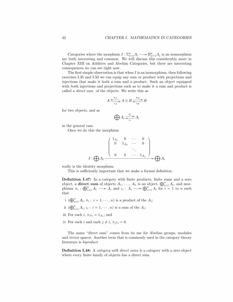
42 CHAPTER I. MATHEMATICS IN CATEGORIES
Categories where the morphism I : Σni=1Ai// Πnj=1Aj is an isomorphism
are both interesting and common. We will discuss this considerably more inChapter XIII on Additive and Abelian Categories, but there are interestingconsequences we can see right now.
The first simple observation is that when I is an isomorphism, then followingexercises I.35 and I.50 we can equip any sum or product with projections andinjections that make it both a sum and a product. Such an object equippedwith both injections and projections such as to make it a sum and product iscalled a direct sum of the objects. We write this as
A oo πA
ιA// A⊕B
πB //ooιB
B
for two objects, and as ⊕Ai
πi //ooιi
Ai
in the general case.Once we do this the morphism
I :⊕
Ai
0BBBBBB@1A1 0 · · · 00 1A2 · · · 0
. . .0 0 · · · 1An
1CCCCCCA//⊕
Ai
really is the identity morphism.This is sufficiently important that we make a formal definition.
Definition I.47: In a category with finite products, finite sums and a zeroobject, a direct sum of objects A1, . . . , An is an object,
⊕ni=1Ai, and mor-
phisms πi :⊕n
i=1Ai// Ai and ιi : Ai // ⊕n
i=1Ai for i = 1 to n suchthat
i (⊕n
i=1Ai, πi : i = 1, · · · , n) is a product of the Ai;
ii (⊕n
i=1Ai, ιi : i = 1, · · · , n) is a sum of the Ai;
iii For each i, πiιi = 1Ai ; and
iv For each i and each j 6= i, πjιi = 0.
The name “direct sum” comes from its use for Abelian groups, modulesand vector spaces. Another term that is commonly used in the category theoryliterature is biproduct.
Definition I.48: A category with direct sums is a category with a zero objectwhere every finite family of objects has a direct sum.

I.3. SPECIAL OBJECTS 43
There is no common name for this type of category, though Lawvere [43] hasargued for “linear category” largely because of results such as those expoundedin this section. That name is not adopted here because it is not commonly used,and because linear category is also used in the literature for at least two othertypes of categories.
Just as with products (I.38) and sums (I.40), the zero object in such acategory is sensibly considered to be the direct sum of zero objects. Contrastthis with exercises I.38 and I.53.
In direct analogy with products and sums we will write the direct sum oftwo objects as (A⊕B, πA, πB , ιA, ιB).
Each projection πi :⊕n
i=1Ai// Ai has the corresponding injection
ιi : Ai // ⊕ni=1Ai as a section (and the injection has the projection as
a retract), so the projections are always epimorphisms, and the injections arealways monomorphisms.
Now for any two morphisms f : A // B and g : C // D, we havealready defined f × g : A×B // C ×C and f + g : A+B // C +D. Butwhen we have direct sums, that means they both are morphisms from A⊕B toC⊕D and so both are given by 2×2-matrices. So what is the matrix for f×g?Well we know that f × g is the unique morphism with πB(f × g) = fπA andπD(f × g) = gπB . To compute the matrix we need πC(f × g)ιA, πC(f × g)ιB ,πD(f × g)ιA, and πD(f × g)ιB . But πC(f × g)ιA = fπAιA = f1A = f andπC(f × g)ιB = fπAιB = f0 = 0. A similar computation for the other twoshows that the matrix is (
f 00 g
)
Exercise I.77. By means of a similar computation show that the matrix off + g is the same as the matrix of f × g, so f + g = f × g.
And so from now on we will write f⊕g : A⊕B // C⊕D in this situation.Also we want to write
⊕ni=1 fi :
⊕ni=1Ai
// ⊕ni=1Bi so we need the more
general result of the next exercise.
Exercise I.78. In a category with direct sums, verify that the matrix of bothΠni=1fi :
⊕ni=1Ai
// ⊕ni=1Bi and Σni=1fi :
⊕ni=1Ai
// ⊕ni=1Bi is
f1 0 · · · 00 f2 · · · 0
. . .0 0 · · · fn
What makes ordinary matrices interesting is primarily that they can be
multiplied, and that multiplication of matrices corresponds to composition ofthe corresponding maps, as is the case for the category of vector spaces. In

44 CHAPTER I. MATHEMATICS IN CATEGORIES
order to define multiplication of these new matrices, we may be able to usecomposition of morphisms in place of multiplication, but what is to take theplace of sum? We actually have a pair of candidates which we will see are actu-ally the same. As we will see in a bit this has several important consequences,and is not at all just a happy accident.
The two “sums” we define on Hom(A,B) are:For f, g ∈ Hom(A,B), define
Definition I.49:
f M g = A∆ // A⊕A
[f,g] // B
and
Definition I.50: fOg = A〈f,g〉 // B ⊕B ∇ // B
Exercise I.79. In the category Ab of Abelian groups, what are (f M g)(a)and (fOg)(a)?
Proposition I.4 In any category with direct sums M and O are the same bi-nary operations on Hom(A,B)
Proof: For f , g in Hom(A,B),
f M g = [f, g]∆ by definition I.49= ∇(f + g)∆ by exercise I.61= ∇(f × g)∆ by exercise I.77= ∇〈f, g〉 by exercise I.46= fOg by definition I.50
Definition I.51: For any category with direct sums and any two morphismsf, g : A // B in the category we define f + g = ∇(f ⊕g)∆. By the precedingproposition f + g = f M g = fOg.

I.3. SPECIAL OBJECTS 45
Exercise I.80. In any category with direct sums, show that for any morphismf , f + 0 = f = 0 + f .Hint: Explain and use the following commutative diagram.
A 0! // 0
B
!
???????????
A
A
1
??A⊕A
A
πA
OO 0
0⊕A
ι0
A A⊕A∆ // A⊕A 0⊕A
!⊕1 // 0⊕A B[!,f //]A
A
1
??????????? A⊕A
A
πA
A
0⊕A
ιA
OO
A A1 // A
B
f
??
Exercise I.81. In any category with direct sums, consider morphisms wherehf , hg, f + g, fe and ge are all defined. Show that h(f + g) = hf + hg and(f + g)e = fe+ ge.
Using this exercise you can readily verify a result that is quite familiar forAbelian groups, vector spaces, etc.
Exercise I.82. In any category with direct sums, show that for any directsum A⊕B we have ιAπA + ιBπB = 1A⊕B
This exercise also allows us to get back to the motivation for the develop-ment of the sum of morphisms: composition of matrices of morphisms.
Proposition I.5 In any category with direct sums, the composition
n⊕i=i
Ai
0BBBBBB@f11 f12 · · · f1m
f21 f22 · · · f2m
. . .fn1 fn2 · · · fnm
1CCCCCCA//m⊕j=1
Bj
0BBBBBB@g11 g12 · · · g1p
g21 g22 · · · g2p
. . .gm1 gm2 · · · gmp
1CCCCCCA//p⊕k=1
Ck
is the n× p-matrix (hik) with hik =g1k
g2k
...gmk
〈fi1, fi2, · · · , fim〉

46 CHAPTER I. MATHEMATICS IN CATEGORIES
Proof: To simplify the notation, we will write F for the matrix (fij), G forthe matrix (gjk) and H for the matrix (hik). Remember that hik = πkHιi =πkGFιi. But πkG is [g1k, · · · , gnk] and Fιi is 〈fi1, fi2, · · · , fim〉.
Now one more proposition will take us to our target.
Proposition I.6 In any category with direct sums, the composition
A〈f1,··· ,fm〉 //
m⊕j=1
Bj[g1,··· ,gm] // C
is g1f1 + · · ·+ gmfm
Unfortunately there is a problem. We have not defined the sum of morethan two morphisms – well so what, we certainly know how to iterate sumsas (((f + g) + h) + k), etc. Unfortunately we don’t yet know that our “sum”is associative! So we need a bit of a detour to fix these details, and the firststep is some convenient notation – for any object, A, we write An for
⊕n1 A.
(Compare the notation An on page 24 and n •A on page 31.)
Definition I.52: In any category with direct sums and any finite number ofmorphisms f1, · · · , fn, all from A to B we define f1 + · · ·+ fn to be
A∆ // An
f1⊕···⊕fn // Bn∇ // B
Now we have a definition, but we really want to know that this sum isassociative. The proof of that is tricky, and we will actually defer it to thediscussion preceding corollary 1 on page 54.
Proof of Proposition I.6 Now of course we have things arranged so thatthe proof is trivial.
[g1, · · · , gm]〈f1, · · · , fm〉 = ∇(g1 ⊕ · · · ⊕ gm)(f1 ⊕ · · · ⊕ fm)∆= ∇(g1f1 ⊕ · · · ⊕ gmfm)∆= g1f1 + · · ·+ gmfm
With the first aspects of “matrix multiplication” in hand, there are manyadditional developments possible, but this is a good point to change our pointof view a bit and consider doing various types of algebra in other categories.Once we have some of that in hand we’ll revisit matrices of morphisms as anapplication and see how it connects to what we have just done.
I.4 Algebraic Objects
A recurring theme in these notes is moving back and forth between investigatingwhat we can do using familiar concepts in general categories as a way to study

I.4. ALGEBRAIC OBJECTS 47
categories (as in the previous section where we found that arbitrary categorieswith finite direct sums have many familiar properties), and using categoriesto investigate familiar concepts (as we are about to do in this section.) Manyfamiliar algebraic structures, such as groups and rings, can be defined in verygeneral categories. Specialized to familiar categories they then give us newinsights and connections.
We will actually return to this theme several times, particularly in Chap-ter VII (Algebraic Categories). This first discussion is largely based on thetreatment given by Eckmann and Hilton [17, 18, 19].
I.4.1 Magmas in a Category
We start with the simplest of algebraic gadgets because it will serve as a usefulbase for most of what follows, and because it usefully simplifies what we needto do. Unfortunately the simplest algebraic gadget is also an unfamiliar one.It is so simple that it really has little interesting theory of its own.
Following Bourbaki [10, I.1] we have the most basic definition.
Definition I.53: A magma is a set, M , together with a binary operation orlaw of composition, µ : M ×M // M .
Most commonly the binary operation in a magma is written as µ(m,n) =mn though in particular examples the operation may be written as m + n,m ∗ n, mn or in some quite different fashion.
Here we make NO assumptions about the operation – it need not be as-sociative, commutative, nor have any sort of identities. Stipulating that theoperation is associative, commutative or satisfies some other identities resultsin other, often more familiar, objects.
Now as we are discussing categories we immediately want to define a suitablemorphism.
Definition I.54: A magma homomorphism is a function f : M // Nsuch that f(xy) = f(x)f(y).
Formally, if (M , µM ) and (N , µN ) are magmas, then a magma homo-morphism f : (M,µM ) // (N,µN ) is a function f : M // N such thatf(µM (x, y)) = µN (f(x), f(y)) for x, y ∈M .
Now we have the category Magmaof magmas which has as objects allmagmas and as morphisms the magma homomorphisms. (You should convinceyourself that this is indeed a category.) And look at Section B.2.1 in theCatalog of Categories (Appendix B) for more information about this category.
We could now go forward and define commutative magmas, and topologicalmagmas, smooth magmas and many other variations on this theme, therebygetting a plethora of additional categories. But there is a better way.
Let C be any category with finite products.
Definition I.55: A magma in C is an object, M , together with a binary

48 CHAPTER I. MATHEMATICS IN CATEGORIES
operation µ : M ×M // M .
And to go along we define the corresponding morphisms.
Definition I.56: A magma morphism, or morphism of magmas in C isa morphism h : M // N such that
M Nh
//
M ×M
M
µM
M ×M N ×Nh×h // N ×N
N
µN
Exercise I.83. Show that there is a category, MagmaC , with objects themagmas in C and as morphisms the magma morphisms.
Of course MagmaSet = Magma, as defined in Section B.2.1.Now we have such categories as MagmaTop, the category of continuous
magmas, and MagmaManifold, the category of smooth magmas.The category MagmaC directly inherits some properties from the mother
category C . First note that if 1 is a final object in C then the unique morphism! : 1 × 1 // 1 exhibits 1 as an object in MagmaC . Moreover for any othermagma, (M,µ) in C clearly
M 1!
//
M ×M
M
µM
M ×M 1× 1!×! // 1× 1
1
!
commutes, so ! is the unique magma morphism from M to 1. Thus 1 (with itsunique binary operation) is also a final object in MagmaC .
Also if M1, . . . , Mn are magmas in C (with binary operations µ1, . . . , µn),then we can use the µi to define a binary operation, µ, on Πn
1Mi. This is doneusing the isomorphism between Πn
1Mi×Πn1Mi and Πn
1 (Mi×Mi) which is givenby exercise I.37. Because we will use this particular isomorphism repeatedly itis worthwhile to make it explicit. It is
〈〈π1, π1〉, · · · , 〈πn, πn〉〉 : Πni=1Mi ×Πn
i=1Mi// Πni=1(Mi ×Mi)
While the inverse is〈〈π1, · · · , πn〉, 〈π1, · · · , πn〉〉
.

I.4. ALGEBRAIC OBJECTS 49
Now we define µ to be the composition of Πn1Mi×Πn
1Mi
∼= // Πn1 (Mi×Mi)
and Πn1µi : Πn
1 (Mi × Mi) // Πn1Mi. Some diagram chasing leads to the
conclusion that (Πn1Mi, µ) is the product of the (Mi, µi) in MagmaC . The
details are in the following exercise.
Exercise I.84. Prove that if C is any category with finite products, thenMagmaC is a category with finite products.
Now we want to preview a bit of what we will start doing once we introducefunctors, the morphisms between categories (cf. Chapter III (Functors).)
Recall that we write Hom(A,B) for the set of morphisms from A to B(orC (A,B) if we want to emphasize which category is being discussed.) More-over we have Hom(C,A × B) ∼= Hom(C,A) × Hom(C,B) (look back at page25.) Lets apply that to a magma (M , µ) and notice that for any objectC we get a binary operation, O, on Hom(C,M) defined by fOg = µ〈f, g〉Even more, if h : M // N is a magma morphism, then the induced functionh∗ : Hom(C,M) // Hom(C,N)is a magma homomorphism.
Exercise I.85. Verify the above assertion that if h : M // N is a magmamorphism, then h∗ is a magma homomorphism.
Now if h : D // C is any morphism in the category, we also have theinduced function h∗ : Hom(C,M) // Hom(D,M).Recalling exercise I.45 wehave the following closely related exercise.
Exercise I.86. Verify that if M is a magma in C , and h : D // C is anymorphism, then h∗ : Hom(C,M) // Hom(D,M) is a magma homomorphism.
One of the motivating examples for this discussion of magmas is the codi-agonal ∇ : A ⊕ A // A in any category with direct sums. In particular thedefinition of O in Hom(A,B) given in Definition I.50 and several of the resultsfollowing that definition are special cases of the material in this section. Andpretty much all of them will be included once we combine the material herewith that in the next section.
Before we move on to that, we want to record the following theorem.
Theorem I.1 Let M be an object in C and suppose that for every object C inC a binary operation, O, is defined on Hom(C,M) in such a way that for ev-ery morphism h : C // D the function h∗ : Hom(D,M) // Hom(C,M) is amagma homomorphism. Then there is a unique binary operation µ : M ×M // Mso fOg = µ〈f, g〉 for all f and g in Hom(C,M)
Proof: Consider µ = π1Oπ2 : M×M // M . Then for f and g in Hom(C,M)

50 CHAPTER I. MATHEMATICS IN CATEGORIES
we have 〈f, g〉 : C × C // M and
µ〈f, g〉 = (π1Oπ2)〈f, g〉= 〈f, g〉∗(π1Oπ2)= 〈f, g〉∗(π1)O〈f, g〉∗(π2)= π1〈f, g〉Oπ2〈f, g〉= fOg
And if ν is some binary operation on M that induces O, then
µ = π1Oπ2
= ν〈π1, π2〉= ν1M×M= ν
Many interesting categories have the property that the Hom sets can benaturally considered as objects in some category other than Set. The study ofsuch categories and the consequences of the additional structure is the subjectof Enriched Category Theory which is the topic of Chapter XII.
I.4.2 Comagmas in a Category
As with just about everything in category theory (and as we will explore morefully in Section II.1)there is a dual to the concept of magma. We are goingstraight to the “categorical” definition for reasons that should be clear veryquickly.
Let C be any category with finite sums. The dual of the magmas arecomagmas. Here is the definition.
Definition I.57: A comagma in C is an object, C, together with a co-operationν : C + C // C.
And to go with it, here is the definition of the appropriate morphisms.
Definition I.58: A comagma morphism, or morphism of comagmas inC is a morphism h : D // C such that
C Dooh
C + C
C
OO
νC
C + C D +Doo h+hD +D
D
OO
νD

I.4. ALGEBRAIC OBJECTS 51
Exercise I.87. Show that there is a category, ComagmaC , with objects thecomagmas in C and as morphisms the comagma morphisms. (Compare toexercise I.83.)
We now have, in particular, the category Comagma = ComagmaSet aswell as many others. Of course the reason that comagmas are actually inter-esting is probably obscure at this point. For instance there are no interestingcomagmas from the category of sets in these notes! Indeed the first interestingspecialization of comagmas is to comonoids, the dual of monoids, But the onlycomonoid in the category of sets is the empty set. (See page 62.) But in timewe will see interesting examples on other categories.
The primary reason that we are discussing comagmas here is because ofwhat happens with Hom.Recall that Hom(A+B,C) ∼= Hom(A,C)×Hom(B,C)(look back at page 32.) Lets apply that to a comagma (C, ν) and notice that forany object B we get a binary operation on Hom(C,B) defined by fOg = [f, g]νEven more, if h : C // D is a comagma morphism, then the induced functionh∗ : Hom(D,B) // Hom(C,B)is a magma homomorphism.
Exercise I.88. Verify the above assertion that if h : C // D is a comagmamorphism, then h∗ is a magma homomorphism. (Compare to exercise I.89.)
Now if h : A // B is any morphism in the category, we also have h∗ :Hom(C,A) // Hom(C,B).Recalling exercise I.60 we have:
Exercise I.89. Verify that if C is a comagma in C , and h : A // B is anymorphism, then h∗ : Hom(C,A) // Hom(D,B)is a magma homomorphism.
The category of comagmas in a category directly inherits some propertiesfrom the mother category. First note that if 0 is a initial object in C the unique
morphism 0 ! // 0 + 0 exhibits 0 as an object in ComagmaC . Moreover forany other comagma, (C, ν) in C clearly
C 0oo!
C + C
C
OO
νC
C + C 0 + 0oo !+!0 + 0
0
OO
!
commutes, so ! is the unique comagma morphism from 0 to C. Thus 0 (withits unique co-operation) is also a initial object in ComagmaC .
Also if C1, . . . , Cn are comagmas in C (with co-operations ν1, . . . , νn),then we can use the νi to define a co-operation, ν, on Σn1Ci by taking ν to bethe composition of
Σni=1νi : Σn1Ci // Σn1 (Ci + Ci)

52 CHAPTER I. MATHEMATICS IN CATEGORIES
andΣn1 (Ci + Ci)
∼= // Σn1Ci + Σn1CiSome diagram chasing leads to the conclusion that (Σn1Ci, ν) is the sum of the(Ci, νi) in ComagmaC . The details are in the next exercise.
Exercise I.90. If C is any category with finite sums, then ComagmaC is acategory with finite sums. (Compare to exercise I.84.)
The motivating example for this discussion of comagmas is the diagonalmorphism ∆ : C // C⊕C in any category with direct sums. In particular thedefinition of M in Hom(A,C) given in I.50 and several of the results followingthat definition are special cases of the material in this section. And prettymuch all of them will be included once we combine the material here with thatin the previous section on magmas.
Before we move on to that, we want to note that if Hom(•,M) is always amagma and gives magma homomorphisms, then M “is” a magma. This easytheorem has a multitude of ramifications.
Theorem I.2 Let C be an object in C and suppose that for every object Ain C a binary operation, M, is defined on Hom(C,A) in such a way that forevery morphism h : A // B the function h∗ : Hom(C,A) // Hom(C,B)is amagma homomorphism. Then there is a unique co-operation ν : C // C +Cso f M g = [f, g]ν for all f and g in Hom(C,A). (Compare to Theorem I.1.)
Proof: Consider ν = ι1 M ι2 : C // C + C. Then for f and g in Hom(C,A)we have [f, g] : C + C // A and
[f, g]ν = [f, g](ι1 M ι2)= [f, g]∗(ι1 M ι2)= [f, g]∗(ι1) M [f, g]∗(ι2)= [f, g]ι1 M [f, g]ι2= f M g
And if µ is some co-operation on M that induces M, then
ν = ι1 M ι2
= [ι1, ι2]µ= 1M+Mµ
= µ
Again note the great similarity (or more precisely the duality) of everythingwe’ve done to this point in this section with what was done in the precedingsection on magmas. This is yet another example of what we will formalize inSection II.1.

I.4. ALGEBRAIC OBJECTS 53
I.4.2.1 Comagmas and Magmas Together
In a category with direct sums, every object naturally has both a magma and acomagma structure, and in Section I.3.3 we saw that the two magma structuresthat were induced on the Hom sets are equal. Here we want to revisit thatmaterial in the context of magmas and comagmas. So suppose that A is acomagma in C with co-operation M (deliberately intended to remind us of thediagonal ∆) and B is a magma in C with binary operation O (deliberatelyintended to remind us of the codiagonal ∇). Then, as above, Hom(A,B) hastwo binary operations M and O defined by
f M g = [f, g] M
hOk = O〈h, k〉
for f , g, h, and k all in Hom(A,B). And these are connected by this masteridentity:
Proposition I.7 (f M h)O(g M k) = (fOg) M (hOk)
Proof:
(f M g)O(h M k) = O〈f M g, h M k〉 by definition of O= O〈[f, g] M, [h, k] M〉 by definition of M= O〈[f, g], [h, k]〉 M by exercise I.89= O[〈f, h〉, 〈g, k〉] M by Proposition I.3= [O〈f, h〉,O〈g, k〉] M by exercise I.86= [fOh, gOk] M by definition of O= (fOh) M (gOk) by definition of M
Now assume that C has a zero object and that the zero morphism inHom(A,B) is the identity for both M and O, i.e., f M 0 = f = 0 M f andgO0 = g = 0Og for all f and g in Hom(A,B). This assumption combined withthe master identity has amazing consequences.
First, taking g = 0 and h = 0, we get
fOk = (f M 0)O(0 M k)= (fO0) M (0Ok)= f M k
i.e., the two binary operations M and O on Hom(A,B). And this means themaster identity can be rewritten as (f + h) + (g + k) = (f + g) + (h+ k)
where + stands for either/both of M and O.

54 CHAPTER I. MATHEMATICS IN CATEGORIES
Part of the reason for using + as the name of the binary operation is becausetaking f = 0 and k = 0 gives
h+ g = (0 + h) + (g + 0)= (0 + g) + (h+ 0)= g + h
i.e., the binary operation is commutative.And finally, taking just h = 0 we get
f + (g + k) = (f + 0) + (g + k)= (f + g) + (0 + k)= (f + g) + k
Which is to say that the two (equal) binary operations on Hom(A,B) are alsoassociative.
Recall that a set together with a binary operation that is associative, com-mutative and has an identity is a commutative monoid, so the above is sum-marized in the following theorem.
Theorem I.3 Let C be a category with a zero object, (A,M) a comagma inC and (B,O) a magma in C such that the zero morphism in Hom(A,B) isthe identity for the binary operations induced by M and O, then the two binaryoperations are the same and make Hom(A,B) a commutative monoid.
As a first consequence we have the following corollary.
Corollary 1 If C is a category with finite direct sums, then for any two objectsA and B in the category, the binary operation on Hom(A,B) defined by thediagonal morphism ∆ and the folding morphism ∇ makes it a commutativemonoid with the zero morphism as the identity.
As another interesting consequence notice that if every object in C admitsa comagma structure and a magma structure such that the 0 morphism is theidentity in the magma structure induced on the Hom sets, then these structuresare necessarily unique. This follows by combining the above proposition withTheorems I.1 and I.2 which say that the magma structure on the Hom setsdetermine the magma and comagmas in C .
In particular this applies to every category with finite direct sums – thecomagma and magma structures defined by ∆ and ∇ are unique!
As a direct lead-in to the next section we have the following summary result.
Proposition I.8 Let C be a category with a zero object, (A,M) a comagma inC and (B,O) a magma in C such that the zero morphism in Hom(A,B) is theidentity for the common binary operation on Hom(A,B), then the followingdiagrams commute:

I.4. ALGEBRAIC OBJECTS 55
1. (B, O) has an identity:
B × 0 B ×B〈π1,0〉 //B × 0
B
π1
$$JJJJJJJJJJJJJJ B ×B
B
O
B ×B 0×Boo 〈0,π2〉B ×B
B
0×B
B
π2
zztttttttttttttt
2. (B, O) is associative:
B ×B BO//
B ×B ×B
B ×B
〈O,1〉
B ×B ×B B ×B〈1,O〉 // B ×B
B
O
3. (B, O) is commutative:
B ×B
B
O
???????????B ×B B ×Bt // B ×B
B
O
4. (A, M) has a co-identity:
A+ 0 A+Aoo [ι1,0]A+ 0
A
dd
ι1
JJJJJJJJJJJJJJ A+A
A
OO
M
A+A 0 +A[0,ι2] //A+A
A
OO 0 +A
A
::
ι2
tttttttttttttt
5. (A, M) is co-associative:
A+A AooM
A+A+A
A+A
OO
[M,1]
A+A+A A+Aoo [1,M]A+A
A
OO
M

56 CHAPTER I. MATHEMATICS IN CATEGORIES
6. (A, M) is co-commutative:
A+A
A
__
M???????????A+A A+Aoo t
A+A
A
??
M
Notation: It occasionally happens that we want to discuss Hom(A,B) wherewe fix B but vary A. Usually the name A just confuses the issue, so in this situa-tion – the following proof is an example – we will often write Hom(•, B)instead.(The notation Hom(−, B) is also sometimes used for the same purpose.) Thissame thing applies for many things besides Hom, and the meaning should beclear in all cases.Proof: For (1.) note that O〈π1, 0〉 = π1 + 0 = π1 and O〈0, π2〉 = 0 + π2 = π2
as 0 is the identity for +, the induced binary operation on Hom(•, B)For (2.) we see that O〈O, 1〉 = O + 1, while O〈1,O〉 = 1 + O. But we know
that + is commutative, so O + 1 = 1 + O.For (3.) we observe that Ot is also a binary operation on B for which 0 is
the identity in the monoid Hom(•, B). But such a binary operation on B isunique, so Ot = O.
We will leave parts (4.) – (6.) as the next exercise.
Exercise I.91. Complete the proof of Proposition I.8
In case they are not clear, the titles for each of the six parts of this propo-sition will be explained in more detail in the next two sections.
I.4.3 Monoids in a Category
Throughout this section all categories are assumed to have finiteproducts.
Definition I.59: A monoid object, or usually just a monoid, in C is amagma in C (M , µ : M ×M // M) plus an identity or unit ζ : 1 // Mfor which the following diagrams commute:
identity
M × 1 M ×M1M×ζ //M × 1
M
π1
$$JJJJJJJJJJJJJJ M ×M
M
µ
M ×M 1×Moo ζ×1MM ×M
M
1×M
M
π2
zztttttttttttttt

I.4. ALGEBRAIC OBJECTS 57
associativity
M ×M Mµ//
M ×M ×M
M ×M
〈µ,1〉
M ×M ×M M ×M〈1,µ〉 // M ×M
M
µ
This definition will likely make more sense when we see that a monoid in Setis just a monoid in the usual sense. Write µ(m,n) = mOn and ζ(∗) = 1 ∈ Mwhere ∗ is the unique element in the singleton set 1. (The use of O for theproduct is intended to remind of the codiagonal, see page 34.) Now the abovediagrams become:
1. identity(m, ∗) (m, 1) //(m, ∗)
m = mO1
??????????(m, 1)
m = mO1
_
(1,m) (∗,m)oo (1,m)
1Om = m
_
(∗,m)
1Om = m
?
2. associativity
(mOn, p) mO(nOp) = (mOn)Op //
(m,n, p)
(mOn, p)
_
(m,n, p) (m,nOp) // (m,nOp)
mO(nOp) = (mOn)Op
_
So the first says that 1 is an identity for the multiplication while the secondis just the associative law for multiplication, i.e., we have a monoid in the usualsense.
In light of the last section we also want to define commutative monoids ina category.
Definition I.60: Let t : M ×M // M ×M be the transposition isomor-phism defined in exercise I.36. A monoid (M , µ, ζ) is commutative iff
M ×M
M
µ
???????????M ×M M ×Mt // M ×M
M
µ
is commutative.

58 CHAPTER I. MATHEMATICS IN CATEGORIES
Note that in Set this just says mOn = nOm, i.e., the multiplication iscommutative in the ordinary sense.
Now we can restate the first three parts of Proposition I.8 as saying thatthe object B is a commutative monoid in the category. The last three parts saythat A is a co-commutative comonoid, and that will be explained and justifiedin the next section.
As we are studying categories, we are, of course, looking for a category ofmonoids, so we want the following definition.
Definition I.61: If (M , µM , ζM ) and (N , µN , ζN ) are two monoids in C ,then a monoid morphism from M to N is a morphism h : M // N in Cfor which the following diagrams commute:
M Nh
//
M ×M
M
µM
M ×M N ×Nh×h // N ×N
N
µN
M N
h//
1
M
ζM
1
N
ζN
???????????
The subscripts on µ and ζ will usually be omitted as the intended subscriptis usually clear from the context.
Again if we look at what this means in the category of sets, then the firstsquare is the familiar h(m M m′) = h(m) M h(m′), while the second is h(1) = 1,exactly what it means for h to be a monoid homomorphism.
Exercise I.92. Show that there is a category, MonoidC , with objects themonoids in C and with morphisms the monoid morphisms.
Of course MonoidSet = Monoid, as defined in Section B.2.3. Well, thereis a tiny issue: the definition of a monoid in Set isn’t exactly the usual definitionof a monoid which just asserts that some identity element exists. Fortunatelyit is an easy theorem that a monoid has a unique identity and so the twoconcepts really do coincide. For more details, see the material on monoidsin Section B.2.3 of the Catalog of Categories. Also look at Mac Lane andBirkhoff [55, I.11].
Exercise I.93. Show that there is a category with objects the commutativemonoids in C and with morphisms the monoid morphisms between commuta-tive monoids.
Of course you’ve already done much of the work for these last two exercisesin exercise I.83.

I.4. ALGEBRAIC OBJECTS 59
This exercise is really about showing that the category of commutativemonoids in C is a subcategory of the category of monoids in C .
Just as with the category of magmas in a category, the category MonoidC
directly inherits various properties from C . Again you’ve already done most ofthe next exercise in exercise I.84.
Exercise I.94. Prove that if C is any category with finite products, thenMonoidC is a category with finite products.
Similarly for the next two exercises, you did most of the work back inexercises I.85 and I.86.
To start, for any monoid (M , µ, ζ) and any object C, the Hom set Hom(C,M)is naturally a monoid with binary operation O defined by fOg = µ〈f, g〉. Theidentity is e = ζ∗(!) ∈ Hom(C,M). [Remember that Hom(C, 1) has just theone element ! as 1 is a final object in C .]
Of course we need to verify the identity and associativity relations forHom(C,M) and that is easily done by noting that the Hom(C, •) operationapplied to the diagrams for M become (writing H for Hom(C,M)):
1. identity
H × 1 H ×H1H×ζ //H × 1
H
π1
$$JJJJJJJJJJJJJJ H ×H
H
µ∗
H ×H 1×Hoo ζ∗×1HH ×H
H
1×H
H
π2
zztttttttttttttt
2. associativity
H ×H Hµ∗//
H ×H ×H
H ×H
〈µ∗,1〉
H ×H ×H H ×H〈1,µ∗〉 // H ×H
H
µ∗
and, as we saw on page 57 these really are the same as the ordinary definitionof a monoid.
Even more, if h : M // N is a monoid morphism, then the inducedfunction h∗ : Hom(C,M) // Hom(C,N)is a monoid homomorphism.
Exercise I.95. Verify the above assertion that if h : M // N is a monoidmorphism, then Hom(C, h) is a monoid homomorphism.
Exercise I.96. Verify that if M is a monoid in C , and h : D // C isany morphism, then h∗ : Hom(C,M) // Hom(D,M) is a monoid homomor-phism.
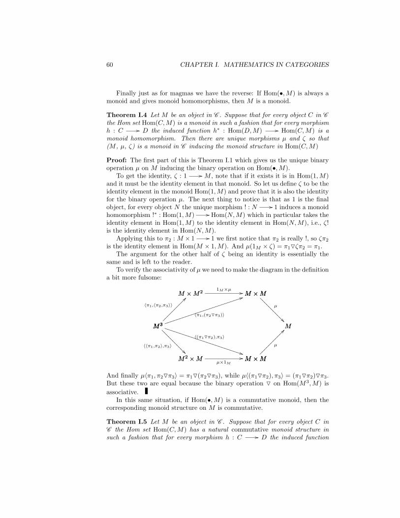
60 CHAPTER I. MATHEMATICS IN CATEGORIES
Finally just as for magmas we have the reverse: If Hom(•,M) is always amonoid and gives monoid homomorphisms, then M is a monoid.
Theorem I.4 Let M be an object in C . Suppose that for every object C in Cthe Hom set Hom(C,M) is a monoid in such a fashion that for every morphismh : C // D the induced function h∗ : Hom(D,M) // Hom(C,M) is amonoid homomorphism. Then there are unique morphisms µ and ζ so that(M , µ, ζ) is a monoid in C inducing the monoid structure in Hom(C,M)
Proof: The first part of this is Theorem I.1 which gives us the unique binaryoperation µ on M inducing the binary operation on Hom(•,M).
To get the identity, ζ : 1 // M , note that if it exists it is in Hom(1,M)and it must be the identity element in that monoid. So let us define ζ to be theidentity element in the monoid Hom(1,M) and prove that it is also the identityfor the binary operation µ. The next thing to notice is that as 1 is the finalobject, for every object N the unique morphism ! : N // 1 induces a monoidhomomorphism !∗ : Hom(1,M) // Hom(N,M) which in particular takes theidentity element in Hom(1,M) to the identity element in Hom(N,M), i.e., ζ!is the identity element in Hom(N,M).
Applying this to π2 : M × 1 // 1 we first notice that π2 is really !, so ζπ2
is the identity element in Hom(M × 1,M). And µ(1M × ζ) = π1Oζπ2 = π1.The argument for the other half of ζ being an identity is essentially the
same and is left to the reader.To verify the associativity of µ we need to make the diagram in the definition
a bit more fulsome:
M ×M
M
µ
???????????M ×M2 M ×M1M×µ //
M3
M ×M
〈π1,(π2Oπ3)〉
44jjjjjjjjjjjjjjjjjjjjjjjjjjM3
M ×M2
〈π1,〈π2,π3〉〉
??M3
M2 ×M
〈〈π1,π2〉,π3〉???????????M3
M ×M
〈(π1Oπ2),π3〉
**TTTTTTTTTTTTTTTTTTTTTTTTTT
M2 ×M M ×Mµ×1M
// M ×M
M
µ
??
And finally µ〈π1, π2Oπ3〉 = π1O(π2Oπ3), while µ〈(π1Oπ2), π3〉 = (π1Oπ2)Oπ3.But these two are equal because the binary operation O on Hom(M3,M) isassociative.
In this same situation, if Hom(•,M) is a commutative monoid, then thecorresponding monoid structure on M is commutative.
Theorem I.5 Let M be an object in C . Suppose that for every object C inC the Hom set Hom(C,M) has a natural commutative monoid structure insuch a fashion that for every morphism h : C // D the induced function

I.4. ALGEBRAIC OBJECTS 61
h∗ : Hom(D,M) // Hom(C,M) is a monoid homomorphism. Then thereare unique morphisms µ and ζ so that (M , µ, ζ) is a commutative monoid inC inducing the monoid structure in Hom(C,M)
Exercise I.97. Prove Theorem I.5
As promised we now have an alternative proof of the first three parts ofProposition I.8 on page 54. Indeed this can be recast as saying that when C isa category with a zero object, (A, M) is a comagma in C , (B, O) a magma inC , and the zero morphism in Hom(A,B) is the identity for the common binaryoperation on Hom(A,B), then (B, O, 0) is a commutative monoid.
The last three parts say that (A, M, 0) is a co-commutative comonoid, andthe next section explains and justifies this claim.
I.4.4 Comonoids in a Category
Even though the definition of duality in categories is still to come in Section II.1,the many examples to date should make it clear that every thing in the previoussection can be “dualized”. We will take advantage of that to leave all the resultsin this section as exercises.
To start we make assume the dual of the presumption of section I.4.3.Throughout this section all categories are assumed to have finitesums.
If you find any of this confusing, you should be able to read ahead in Section II.1as well as reading the solutions.
Definition I.62: Suppose C is a category with finite sums. A comonoidobject or usually just a comonoid in C consists of an object C and morphismsν : C // C+C and η : C // 0 so that (C, ν) is a comagma and the followingdiagram commutes:
C + 0 C + Coo [ι1,η]C + 0
C
dd
ι1
JJJJJJJJJJJJJJ C + C
C
OO
O
C + C 0 + C[η,ι2] //C + C
C
OO 0 + C
C
::
ι2
tttttttttttttt
Terminology: We will often just speak of a comonoid or a comonoid objectif the category is clear. The morphism ν is, of course, called the comultipli-cation,while η is called the co-unitof the comonoid.
While for monoids we were able to explain the definition of a monoid objectby pointing out that it was familiar in the category of sets, we don’t have thatadvantage with comonoids. Comonoids are not familiar, and in the category

62 CHAPTER I. MATHEMATICS IN CATEGORIES
of sets there is only one comonoid, namely the empty set! So for the momentthis is largely an exercise in formal manipulation, with a promise that this willbe more interesting later on
Definition I.63: Let t : C + C // C + C be the transposition isomorphis-mdefined in definition I.32 on 32. A co-monoid (C, ν, η) is co-commutativeiff
C + C
C
__
ν???????????C + C C + Coo t
C + C
C
??
ν
is commutative.
Now see that the second three parts of Proposition I.8 does just say that Ais a co-commutative comonoid.
As we are studying categories, we are, of course, looking for a category ofcomonoids, so we want the following definition.
Definition I.64: If (C, ν, η) and (D, ν, η) are two comonoids in C , thena comonoid morphism from C to D is a morphism h : C // D in C forwhich the following diagrams commute:
C Dooh
C + C
C
OO
ν
C + C D +Doo h+hD +D
D
OO
ν
C Dooh
1
C
??
η
1
D
__
η
???????????
Exercise I.98. Show that there is a category, ComonoidC , with objects thecomonoids in C and as morphisms the comonoid morphisms.
Exercise I.99. Show that there is a category with objects the co-commutativecomonoids in C and as morphisms the comonoid morphisms between co-commutative comonoids.
Of course you’ve already done most of the work for these two exercises inexercise I.87.
Just as with the category of comagmas in a category, the category ComonoidC
directly inherits various properties from C . Again you’ve already done most ofthe next exercise in exercise I.90.
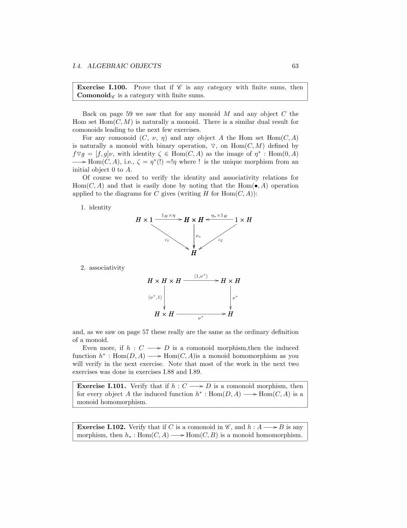
I.4. ALGEBRAIC OBJECTS 63
Exercise I.100. Prove that if C is any category with finite sums, thenComonoidC is a category with finite sums.
Back on page 59 we saw that for any monoid M and any object C theHom set Hom(C,M) is naturally a monoid. There is a similar dual result forcomonoids leading to the next few exercises.
For any comonoid (C, ν, η) and any object A the Hom set Hom(C,A)is naturally a monoid with binary operation, O, on Hom(C,M) defined byfOg = [f, g]ν, with identity ζ ∈ Hom(C,A) as the image of η∗ : Hom(0, A)
// Hom(C,A), i.e., ζ = η∗(!) =!η where ! is the unique morphism from aninitial object 0 to A.
Of course we need to verify the identity and associativity relations forHom(C,A) and that is easily done by noting that the Hom(•, A) operationapplied to the diagrams for C gives (writing H for Hom(C,A)):
1. identity
H × 1 H ×H1H×η //H × 1
H
ι1
$$JJJJJJJJJJJJJJ H ×H
H
ν∗
H ×H 1×Hoo η∗×1HH ×H
H
1×H
H
ι2
zztttttttttttttt
2. associativity
H ×H Hν∗
//
H ×H ×H
H ×H
〈ν∗,1〉
H ×H ×H H ×H〈1,ν∗〉 // H ×H
H
ν∗
and, as we saw on page 57 these really are the same as the ordinary definitionof a monoid.
Even more, if h : C // D is a comonoid morphism,then the inducedfunction h∗ : Hom(D,A) // Hom(C,A)is a monoid homomorphism as youwill verify in the next exercise. Note that most of the work in the next twoexercises was done in exercises I.88 and I.89.
Exercise I.101. Verify that if h : C // D is a comonoid morphism, thenfor every object A the induced function h∗ : Hom(D,A) // Hom(C,A) is amonoid homomorphism.
Exercise I.102. Verify that if C is a comonoid in C , and h : A // B is anymorphism, then h∗ : Hom(C,A) // Hom(C,B) is a monoid homomorphism.

64 CHAPTER I. MATHEMATICS IN CATEGORIES
And finally we have the is dual of Theorem I.4 on page 60, the resultfor Hom and monoids: If Hom(C, •) is always a monoid and gives monoidhomomorphisms, then C is a comonoid.
Theorem I.6 Let C be an object in C . Suppose that for every object A in Cthe Hom set Hom(C,A) is a monoid in such a way that for every morphismh : A // B the induced function h∗ : Hom(C,A) // Hom(C,B) is a monoidhomomorphism. Then there are unique morphisms ν and η so that (C, ν, η)is a comonoid in C inducing the monoid structure in Hom(C,A)
Exercise I.103. Prove Theorem I.6
In this same situation, if Hom(C, •) is a commutative monoid, then thecorresponding comonoid structure on C is co-commutative.
Theorem I.7 Let C be an object in C . Suppose that for every object A in Cthe Hom set Hom(C,A) is a commutative monoid in such a way that for everymorphism h : A // B the induced function h∗ : Hom(C,A) // Hom(C,B)is a monoid homomorphism. Then there are unique morphisms ν and η so that(C, ν, η) is a co-commutative comonoid in C inducing the monoid structurein Hom(C,A)
Exercise I.104. Prove Theorem I.7
As promised we now have an alternative proof of the second part of Propo-sition I.8. Indeed this can now be recast as saying that when C is a categorywith a zero object, (A, M) is a comagma in C and (B, ν) a magma in C suchthat the zero morphism in Hom(A,B) is the identity for the common binaryoperation on Hom(A,B), then (A, M, 0) is a co-commutative comonoid.
Now as you may have guessed we could continue on to define monoidsacting on other objects, or rings or other algebraic gadgets in quite generalcategories in much the same way we done with magmas and monoids. Butwe’ll postpone that until we have more machinery that will simplify the processconsiderably (see Chapter VII, Algebraic Categories.) But we do want to lookat the categorical generalization of one of the most familiar concepts: groups.
I.4.5 Groups in a Category
A group is a monoid in which every element has an inverse. The correspondingdefinition in a category is the following.
Definition I.65: Suppose C is a category with finite products. A groupobject or usually just a group in C consists of an object G and morphisms

I.4. ALGEBRAIC OBJECTS 65
µ : G×G // G, ζ : 1 // G, and ι : G // G so that (G, µ, ζ) is a monoidin C and ι is the inverse. This mean that the following diagrams commute:
1 Gζ
//
G
1
!
G G×G〈1G,ι〉 // G×G
GG 1oo
ζ
G×G
G
µ
G×G Goo 〈ι,1G〉G
1
!
Of course this is really just saying that a group object is a monoid objecttogether with an inverse, in particular in the category of sets ι : G // G isjust ι(g) = g−1.
Now we can go one step further and define the corresponding morphisms.
Definition I.66: If (G, µ, ζ, ι) and (H, µ, ζ, ι) are two groups in C , then agroup morphism from G to H is a morphism h : G // H in C for whichthe following diagrams commute:
G Hh
//
G×G
G
µ
G×G H ×Hh×h // H ×H
H
µ
G H
h//
1
G
ζ
1
H
ζ
???????????
G Hh
//
G
G
ι
G Hh // H
H
ι
As you should expect this is a monoid homomorphism that also “carriesinverses to inverses”, the natural generalization from Set.
We call also easily define Abelian, i.e., commutative, groups.
Definition I.67: A group (G, µ, ζ, ι) is commutative or Abelian iff themonoid (G, µ, ζ) is commutative.
In the next exercise you will show that there is a category of groups in C .Of course most of the work was already done in exercise I.92
Exercise I.105. Show that there is a category, GroupC , with objects thegroups in C and as morphisms the group morphisms.

66 CHAPTER I. MATHEMATICS IN CATEGORIES
Of course GroupSet = Group, as defined in Section B.2.5, right? Well,there is actually a bit to be said here. The issue is that the definition of a groupin Set does not immediately translate into the usual definition of a group. Forexample in their book Algebra [55], Mac Lane and Birkhoff give the definition:“A group G is a set G together with a binary operation G×G // G, written(a, b) 7→ ab such that
i This operation is associative.ii There is an element u ∈ G with ua = a = au for all a ∈ G.iii For this element u, there is to each element a ∈ G an element a′ ∈ G with
aa′ = u = a′a.Now even though this was written by Saunders Mac Lane, one of the fathers
of category theory, there is no mention of the functions ζ and ι that are partof our definition of a group in the category Set! Of course the existence of theelement u guaranteed by the above definition allows us to define the functionζ : 1 // G by ζ(∗) = u. But a priori it appears that a group in the abovesense might allow several different such elements u and therefor several differentgroup objects in Set. Of course this is not the case as it is an easy theoremthat there is only one such element u.
Similarly the existence for each a ∈ G of a′ with aa′ = u = a′a allows us(perhaps with the aid of the axiom of choice!) to define an ι : G // G so thataι(a) = u = ι(a)a. Again there is an a priori possibility that there might bemany such functions leading to many different group objects in Set associatedto a particular group. But again this is not in fact the case as another easytheorem shows that such an element a′ is unique for each a and so there is onlyone such function ι (and the axiom of choice is not needed.)
For more details, see the material on groups in Section B.2.5 of the Catalogof Categories. Also look at Mac Lane and Birkhoff [55, II].
This kind of issue comes up rather regularly when moving between thestandard set based definitions and those reformulated to fit category theory.In these early stages we will usually write a bit about the issues, but thenwe will leave it to the reader without comment unless there are particularlyinteresting issues.
There is also the category of Abelian groups in C which is a subcategoryof the category of groups in C . That’s the content of the next exercise whereyou’ve already done the work for in the last exercise and in exercise I.93.
Exercise I.106. Show that there is a category with objects the commutativegroups in C and as morphisms the group morphisms between commutativegroups.
This is an opportunity to point out a subtlety that occasionally confusesnewcomers to category theory. With the usual definition of groups and monoids(that is as sets with a binary operation), it is quite true that the category ofgroups is a subcategory of the category of monoids. But if we look at the

I.4. ALGEBRAIC OBJECTS 67
definition we have given of monoid and group in the category Set, it is nottrue that every group is a monoid! The reason for this is that each group hasthe inverse function (ι) in addition to binary operation (µ) and the identity(ζ). In principal it might be the case that we could have two group objects(G, µ, ζ, ι) and (G, µ, ζ, γ) where the only difference is the inverse morphism.In the category of sets this cannot happen – we know that if an element in amonoid has an inverse, the inverse is unique – and that is why the category ofgroups is a subcategory of the category of monoids. In a general category withfinite products there are no elements to have inverses, unique or no. Indeedthe role of objects in categories is a very secondary one, so the notion of asubcategory is interesting primarily for the examples arising as subcategoriesof familiar categories. Even more interesting is the situation illustrated by therelations between magmas, monoids and groups in a category. Every groupobject does have an underlying monoid object, and each monoid object has anunderlying magma object – in both cases the underlying object is gotten bysimply “forgetting” the extra structure, i.e., the underlying monoid of a groupis gotten by forgetting the inverse, while the underlying magma of a monoidis gotten by forgetting the identity. Moreover the group morphisms betweentwo group objects is a subset of the monoid homomorphisms between the twounderlying monoids, and equally well a subset of the magma homomorphismbetween the two underlying magmas. This is a very common situation and iscodified in the discussion of based categories and forgetful functors coming upin Sections II.5 and III.2.6.
Just as with the categories of magmas and monoids in a category, thecategory GroupC directly inherits various properties from C . Again you’vealready done most of the next exercise in exercise I.94.
Exercise I.107. Prove that if C is any category with finite products, thenGroupC is a category with finite products.
For any object C and any monoid objectM , the set of morphisms Hom(C,M)is naturally a monoid (see page 59.) Similarly for any group object G, the setof morphisms Hom(C,G) is naturally a group – the multiplication and identitycome from the monoid structure that G gives as a monoid. The inverse onHom(C,G) is just ι∗ where ι is the inverse on G.
Exercise I.108. Verify that ι∗ is indeed the inverse on Hom(C,G) as claimed.
For the next two exercises, most of the work was back in exercises I.95 andI.96.
Exercise I.109. Verify the above assertion that if h : G // H is a groupmorphism, then for any C Hom(•, h) is a group homomorphism.

68 CHAPTER I. MATHEMATICS IN CATEGORIES
Exercise I.110. Verify that if G is a group in C , and h : D // C is anymorphism, then h∗ : Hom(C,G) // Hom(D,G) is a group homomorphism.
Finally we see that, just as for magmas and monoids, if Hom(•, G) is alwaysa group and gives group homomorphisms, then G is a group.
Theorem I.8 Let G be an object in C . Suppose that for every object C inC the Hom set Hom(C,G) is a group in such a way that for every morphismh : C // D the function h∗ : Hom(D,G) // Hom(C,G) is a group homo-morphism. Then there are unique morphisms µ, ζ, and ι so that (G, µ, ζ, ι)is a group in C inducing the group structure in Hom(C,G)
Exercise I.111. Prove Theorem I.8.
Combining this proposition with Theorem I.5 gives us
Theorem I.9 Let G be an object in C . Suppose that for every object C inC the Hom set Hom(C,G) is an Abelian group in such a way that for everymorphism h : C // D the function h∗ : Hom(D,G) // Hom(C,G) isa group homomorphism. Then there are unique morphisms µ, ζ, and ι sothat (G, µ, ζ, ι) is an Abelian group in C inducing the group structure inHom(C,G)
To date we have some of the elementary definitions regarding monoids andgroups, but no actual development of any interesting information about thesecategories themselves, not even such simple results as the isomorphism the-orems for groups. We could in fact develop that material in a fairly directmanner, but it is much more worth while to first develop some of the machin-ery of category theory which we can then apply.

Chapter II
Constructing Categories
Examples of categories abound, and we saw that familiar notions in the cate-gory of sets generalize to other bases categories to give even more categories.But category theory also suggests other ways of getting more categories – prod-ucts and sums of categories, subcategories, quotient categories, functor cate-gories, etc. These are particularly important as a way of organizing complexity,especially when we study functors and functor categories will come in the nextchapter.
II.1 Duality and Dual Category
Two points determine a line and, in the projective plane, two lines alwaysintersect in a point. This is an ancient example of the duality between linesand points with Pappus’ Theorem (see [68]) on nine points and nine lines beingperhaps the first duality theorem. Today there are dozens if not hundreds ofduality theorems in mathematics, many of them key results.
Duality pairs up objects and relations in a complementary fashion so thatthere are dual theorems with dual proofs. The simplest examples of dualityinclude negation of propositions in logic (where for example the “and” oper-ation is dual to “or”), dual polyhedra (see [67]) where faces and vertices areswapped (the dual of the cube is the octahedron; the dual of the dodecahedronis the icosahedron; while the tetrahedron is its own dual), and pairing regionsand vertices in planar graphs.
More sophisticated examples include Poincare Duality (see [4]) in algebraictopology and Pontryagin Duality (see [69]) for topological groups.
Category theory is another area where duality plays an important role.What makes it particularly interesting is that a great many of the other notionsof duality can be expressed by duality for categories. The starting point is thedefinition of the dual of a category.
Definition II.1: Associated to any category C is a dual or opposite categorydenoted C op. The objects and morphisms of C op are exactly the objects and
69

70 CHAPTER II. CONSTRUCTING CATEGORIES
morphisms of C , but f is a morphism from A to B in C iff f is a morphismfrom B to A in C op. Finally composition is reversed in C op from what it isin C . If h = gf in C , then h = fg in C op.
Clearly (C op)op is just C .Although the definition of the dual category is a very simple formality, it has
a great deal of force. The first import is that it reduces the number of proofsin category theory by a factor of 2! The reason for this is that when we provea theorem for all categories, it of course applies not only to each particularcategory, but also to its dual category. But the theorem applied in the dualcategory is (usually) another different theorem in the original category. Hereare some simple examples that where we have already done twice the work thatwas needed.
First we note that section and retract are dual concepts. If f : A // B isa section of g : B // A in C , then f : B // A is a retract of g : A // Bin C op.
CC C opC op
B
A
g
???????????B B1B // B
A
??
f
B
A
__
g
???????????B Boo 1BB
A
f
Similarly epimorphism and monomorphism are dual concepts. If the mor-phism f : A // // B is an epimorphism in C , then f : B // // A is a monomor-phism in C op. If gf = hf ⇒ g = h in C , then fg = fh⇒ g = h in C op (andconversely.)
Next note that final object and initial object are dual concepts, i.e., if Xis a final object in the category C , then X is an initial object in the categoryC op:
CC C opC op
C X! //____ C Xoo ! ____
For each object C there is the unique morphism C // X in C and theunique morphism X // C in C op.
As our final examples for the moment we see that product and sum aredual concepts. Suppose 〈X, a : X // A, b : X // B〉 is a product of A and

II.1. DUALITY AND DUAL CATEGORY 71
B in C , then 〈X, a : A // X, b : B // X〉 is a sum of A and B in C op:
CC C opC op
X
B
b
C X//____C
B
g
???????????
A
C
??
f
A
X
OO
a
X
B
OO
b
C Xoo ____C
B
__
g
???????????
A
C
f
A
X
a
For each pair of morphisms f : C // A and g : C // B in C thereis a unique morphism C // X in C making the left diagram commute, andin C op for each pair of morphisms f : A // C and g : B // C there is aunique morphism X // C making the right diagram commute. We’ve onlyindicated this for pairs of objects, but you should easily see that it is true forarbitrary products and sums as well.
Now consider the following pairs of propositions:
1. a) If a morphism f has a section, then f is an epimorphism. (Seeexercise I.10.)
b) If a morphism f has a retract, then f is a monomorphism. (Seeexercise I.16.)
2. a) (Proposition I.1) If P with πi : P // Ai and P ′ with π′i : P ′// Ai are both products of A1, · · · , An, then 〈π1, · · · , πn〉 : P// P ′ is an isomorphism with 〈π′1, · · · , π′n〉 : P ′ // P as inverse.
b) (Proposition I.2) If S with ιj : Ai // S and S′ with ι′j : Ai // S′
are both sums of A1, · · · , An, then [ι1, · · · , ιn] : S′ // S is anisomorphism with [ι′1, · · · , ι′n] : S // S′ as inverse.
3. a) For any family of two or more objects, A1, · · · , An, in C prove thatΠni=1Ai is isomorphic to Πn−1
i=1 Ai ×An. (See exercise I.34.)
b) For any family of two or more objects, A1, · · · , An, in C prove thatΣni=1Ai is isomorphic to Σn−1
i=1 Ai +An. (See exercise I.49.)
4. a) Suppose f : P // A×B is an isomorphism. Prove that 〈P, π1f, π2f〉is also a product of A and B. (See exercise I.35.)
b) Suppose f : A+B // S is an isomorphism. Prove that 〈S, fι1, fι2〉is also a sum of A and B. (See exercise I.50.)
5. a) Define t : A×B // B ×A by t1 = π2, t2 = π1. Prove that t is anisomorphism. (See exercise I.36.)

72 CHAPTER II. CONSTRUCTING CATEGORIES
b) Define f : A+B // B +A by f1 = ι2, f2 = ι1. Prove that f is anisomorphism. (See exercise I.51.)
6. a) Any two final objects in C are isomorphic, and the isomorphism isunique. (See exercise I.69.)
b) Any two initial objects in C are isomorphic, and the isomorphismis unique. (See exercise I.73.)
7. a) In any category with a final object, 1×A = A. (See exercise I.71.)b) In any category with an initial object, 0 + A = A. (See exercise
I.74.)
These are pairs of dual propositions. In all cases each proposition is a logicalconsequence of the other because each applies equally well to dual categories.In our proofs of these results (most being in the Solutions (Appendix C)), wehave tried to write the proofs to emphasize the duality.Going forward we willprove only one of the dual theorems of interest, and indeed may use the dualtheorem without even explicitly stating it.
There are a number of well known results in mathematics that are trulyabout dual categories. One of the simplest, and one of the motivating examplesin the development of the original definitions of category theory, is that thecategory of finite dimensional vector spaces over a fixed field is self-dual, i.e., itis “equivalent” to its own dual category. To justify that will be one of the earlygoals of Chapter III (Functors).
II.2 Quotient Categories
Besides subgroups, subrings, subspaces, etc., there are also quotient groups,quotient rings, quotient spaces, etc. Similarly there is the notion of a quotientcategory.
The initial motivating examples of quotient categories are the various homo-topy categories in algebraic topology. For more details look at in the Catalog ofCategories at the homotopy category of topological space (B.9.6), the categoryof H-Spaces (B.9.7), the homotopy category of Kan complexes (B.10.2), andthe homotopy category of chain complexes (B.11.4).
As a preliminary to the definition of a quotient category, we need to specifythe kind of equivalence relation that is relevant.
Definition II.2: A congruence ∼on a category is an equivalence relation onthe morphisms in the category such that
i If f ∼ g, then f and g have the same domain and codomain.
ii If f ∼ g and h ∼ k and hf is defined, then hf ∼ kg.
If ∼ is a congruence on the category C , define C / ∼ as the category withthe same objects as C , and with the morphisms from A to B in C / ∼ the

II.3. PRODUCT OF CATEGORIES 73
equivalence classes of C (A,B) with respect to the equivalence relation ∼. Theidentity morphism on A is the equivalence class of 1A, and the compositionof equivalence classes is the equivalence class of the composition of any twomorphisms in the equivalence classes.
Exercise II.1. Verify that C / ∼ as described above is in fact a category.
Definition II.3: C / ∼ is called the quotient category of C by the congruence∼.
II.3 Product of Categories
Along with subcategories and quotient categories, there are also products ofcategories. Here is the definition.
Definition II.4: B are two categories, the product category A ×B hasas objects the pairs (A,B) with A an object of A and B an object of Band asmorphisms the pairs (f, g) with f a morphism in A and g a morphism in B.The domains, codomains, composition, and identities are exactly as expected:if f : A0
// A1 and f ′ : A1// A2 in A while g : B0
// B1 and g′ : B1// B2 in B, then (f, g) : (A0, B0) // (A1, B1) and (f ′, g′) : (A1, B1) //
(A2, B2) in A ×B. Moreover (f ′, g′)(f, g) = (f ′f, g′g) and 1(A,B) = (1A, 1B).The domain of (f, g) is the pair (domain(f), domain(g)) and the cod while
the of objects from A and B respectively, while the morphisms are similarpairs of morphisms.
Exercise II.2. Verify that A ×B is indeed a category.
We’ve only defined the product of two categories, but the definition actuallyextends to the product of any indexed family of categories as follows:
Definition II.5: If (Ci : i ∈ I) is an indexed family of categories with Iany set, then we define the product category Πi∈ICi with the objects beingindexed families of objects (Ci : i ∈ I) and the morphisms being indexedfamilies of of morphisms (fi : i ∈ I).
The only (apparent) issue in this construction is that we are treading closeto foundational issues when the objects in these categories do not form a set.This can be addressed, but we will just refer to the discussions mentionedearlier, cf. page 5.
74 CHAPTER II. CONSTRUCTING CATEGORIES
II.4 Sum of Categories
Besides products of categories there are also sums of categories. Here is thedefinition.
Definition II.6: If (Ci : i ∈ I) is an indexed family of categories with I anyset, then we define a category Σi∈ICi with the objects being pairs (C, i) withi ∈ I and C an object of Ci. There are no morphisms from (C, i) to (D, j)unless i = j in which case every morphism f : C // D in Ci gives a morphism(f, i) : (C, i) // (D, i).
Exercise II.3. Verify that Σi∈ICi, as defined above, is indeed a category.
II.5 Concrete and Based Categories
The overwhelming majority of the familiar categories (see the Catalog of Cat-egories (Appendix B)) come from the category of sets by defining the objectsof the new category as sets with some additional structure (e.g., a binary op-eration [as with Monoid] or a family of subsets [as with Top]), while the newmorphisms are defined to be functions between the sets which in some fashionpreserve the structure.
Rather than trying to specify just what is meant by a structure we willabstract this situation to get the following (tentative) definition.
Definition II.7: A concrete category is a category C and a specification ofthe underlying sets and functions in Set. This last means that for each objectC of C there is specified a set U(C) and each morphism f : C // D of Cthere is a function U(f) : U(C) // U(D). Moreover U has to satisfy someconsistency conditions:
1. U(1C) = 1U(C)
2. U(gf) = U(g)U(f)
3. if f, f ′ : C // D and U(f) = U(f ′), then f = f ′.
The image here is that U(C) is the underlying set of the object, i.e., the setgotten by forgetting about the structure. Similarly U(f) is the function thatpreserves the structure. The three consistency conditions say that the identityfunction preserves the structure, that composition of the morphisms in the newcategory is just composition of functions, and that the only morphisms in thenew category are indeed just suitable functions.
This is labeled a tentative definition because as soon as we have the defini-tion of a functor we will restate this definition and see that U is just a faithful

II.5. CONCRETE AND BASED CATEGORIES 75
functor from C to Set, called the underlying or forgetful functor (details indefinition III.8 and Section III.2.6.)
Exercise II.4. There are many categories listed in the Catalog of Categories(Appendix B) that are quite naturally concrete categories. The first and sim-plest is the category of sets itself. There U is just the identity on objects andmorphisms.Decide which of the categories in the Appendix are naturally concrete categoriesand for those describe a forgetful functor. [This is a trivial exercise, particularlyas the answer in each case is in the article for the given category. It is just anexcuse to get you to review these categories and reflect on concrete categories.Not all of the categories listed are concrete categories, but proving that thereis no forgetful functor can be non-trivial.]
This is also a special case of a more general phenomenon that we saw repeat-edly in Section I.4. Much as with concrete categories, the various categories ofalgebraic objects were constructed from some base category by defining the ob-jects of the new category as objects in the base category with some additionalstructure (e.g., a binary operation as with magmas in a category, MagmaC ),while the new morphisms were defined to be morphisms in the base categorywhich respected the structure.
Again rather than trying to specify just what is meant by a structure wewill abstract this situation to get the following (tentative) definition.
Definition II.8: A based category on a base category B is a category Cand a specification of the objects and morphisms in B. This last means that foreach object C of C there is specified an object U(C) in B and each morphismf : C // D of C there is a morphism U(f) : U(C) // U(D). Moreover Uhas to satisfy the consistency conditions:
1. U(1C) = 1U(C)
2. U(gf) = U(g)U(f)
3. if f, f ′ : C // D and U(f) = U(f ′), then f = f ′.
This too is labeled a tentative definition because it also will be supersededas soon as we have the definition of a functor and can restate this definition assaying that U is just a faithful functor from C to B (details in definition III.8and Section III.2.6.)
The next exercise is just looking at a very few of the multitude of examplesof based categories that will naturally occur in these notes.

76 CHAPTER II. CONSTRUCTING CATEGORIES
Exercise II.5. For each of the following situations, confirm that we do havea based category as asserted. [Again this exercise is trivial and just intendedto get you to reflect on based categories.]
1. Group based on Set
2. Group based on Monoid
3. Monoid based on Magma
4. GroupC based on C
5. GroupC based on MonoidC
6. MonoidC based on MagmaC .
7. MagmaC based on C (see Section I.4.1, in particular exercise I.83.)
8. LieGroup based on Manifold
9. ModuleR based on Ab
II.6 Morphism Categories
For any category there are a variety of associated categories where the ob-jects of the new category are certain morphisms from the original category.Throughout this section let C be a fixed category.
• The first and simplest example is the case where we consider all themorphisms as the objects of our new category. The category C 2, calledthe morphism category of C , has as objects the morphisms of C , whilea morphism in C 2 from f : A // B to f ′ : A′ // B′ is a pair (h, k) ofC -morphisms so that
B B′k
//
A
B
f
A A′h // A′
B′
f ′
commutes.
The identity morphism on f is the pair (1A, 1B), while the composition

II.6. MORPHISM CATEGORIES 77
of (h, k) : f // f ′ with (h′, k′) : f ′ // f” is (h′h, k′k) as in
B B′k
//
A
B
f
A A′h // A′
B′
f ′
B′ B”
k′//
A′
B′
A′
B′
A′ A”h′ // A”
B”
f”
That C 2 is a category follows immediately from the fact that C is acategory.
The explanation for the notation C 2 and the connection with the arrowcategory 2 is in Section III.6.7 below.
• The next interesting case arises when we restrict our morphisms to havea fixed domain. For C a fixed object of C , the Category of objectsunder C, written (C ↓ C ) has as objects morphisms in C with domainC, while a morphism in (C ↓ C ) is a C -morphism between the codomainsthat makes the following triangle commute:
D D′k
//
C
D
f
C
D′
f ′
???????????
So here k is a morphism from f to f ′ in (C ↓ C ).
(C ↓ C ) is immediately seen to be the subcategory of C 2 consisting ofjust those “objects” with domain C and just the “morphisms” of the form(1C , k).
Both objects under C and the following definition of objects over C areexamples of the more general and useful construction of comma cate-gories which will be discussed in Section IV.1 where the notation will beexpanded and discussed.
As an example, considering Set, the category of sets, and C to be a finalobject 1, i.e., any fixed one element set, we see that (Set ↓ 1) is essen-tially the same as the category Set∗ of pointed sets. (Cf. Section I.3.2,especially page 38, and Section B.1.7.) For a function from 1 to any setS is completely determined the point s0 ∈ S (the base point) that is theimage of the function, and a morphism in (Set ↓ 1) is exactly a functionthat takes base point to base point. Formally what we see is that thecategory (Set ↓ 1) is isomorphic to the category Set∗, and this will essen-tially be a proof of that fact as soon as we actually define “isomorphismof category” which we will do in definition III.6 on page 81.

78 CHAPTER II. CONSTRUCTING CATEGORIES
• The dual to the notion of the category of objects under C is of thecategory of objects over C, written (C ↓ C). Here the objects aremorphisms in C with codomain C, and a morphism is a C -morphismbetween the codomains that making the triangle commute:
B
C
g
???????????B B′h // B′
C
g′
Here h is a morphism (in (C ↓ C)) from g to g′.
Again (C ↓ C) is a subcategory of C 2 consisting of just those “objects”with codomain C and just the “morphisms” of the form (h, 1C).
By contrast with (Set ↓ 1), the category (1 ↓ Set) is really the same asSet itself. For any set S there is a unique function from S to 1, and forany function f : S // S′, the triangle
S
1
!
???????????S S′f // S′
1
!
commutes.
This argument really is just using the fact that 1 is a final object in Set.The same argument shows that for any category with final object thecategory (C ↓ 1) is isomorphic to C .
Dually for any category with initial object 0, the category (0 ↓ C ) isisomorphic to C .
Chapter III
Functors and NaturalTransformations
III.1 What is a Functor?
A functor is a morphism from one category to another. Here is the actualdefinition.
Definition III.1: A functor F from C to D assigns to each object A in Can object F (A) in D and to each morphism f : A // B in C a morphismF (f) : F (A) // F (B). Moreover F (1A) = 1F (A) for every object in A in C ,
and whenever Af // B
g // C in C , F (gf) = F (g)F (f) in D .
The canonical examples of functors are C (C, •) : C // Set, the Hom func-tors.For each object A of C we have the set C (C,A) and for each morphism f :A // B we have the function f∗ = Hom(C, f) : Hom(C,A) // Hom(C,B)from Definition I.7. Clearly (1A)∗ is the identity function on C (A,A), and(gf)∗ = g∗f∗ is exactly the associative law in C .
But we have another canonical example: C (•, C) : C // Set. For eachobject A of C we have the set C (A,C) and for each morphism f : A //
B we have the function f∗ = Hom(f, C) : Hom(B,C) // Hom(A,C) fromDefinition I.8. And this is not a functor because (gf)∗ = f∗g∗ rather than(gf)∗ = g∗f∗.
This is sufficiently important that it too gets a definition.
Definition III.2: A contravariant functor F from C to D assigns to eachobject A in C an object F (A) in D and to each morphism f : A // B in C amorphism F (f) : F (B) // F (A). Moreover F (1A) = 1F (A) for every object
in A in C , and whenever Af // B
g // C in C , F (gf) = F (f)F (g) in D .
Sometimes for emphasis a functor is called a covariant functor. To confusethings a bit, a few authors have used the term cofunctor. for contravariant
79

80 CHAPTER III. FUNCTORS AND NATURAL TRANSFORMATIONS
functor.So we also have the contravariant Hom functors C (•, C) : C // Set.As we would expect for “morphisms of categories”, there are identity func-
tors and composition of functors.
Definition III.3: The identity functor 1C : C // C has 1C (C) = C and1C (f) = f for every object C and morphism f in C . This is clearly a functor.
Definition III.4: For two functors F : A // B and G : B // C , thecomposition GF : A // C has GF (A) = G(F (A)) and GF (f) = G(F (f))for every object A and morphism f in A . And again it is clear that thecomposition is a functor.
The same definition applies equally well if either F , G or both are con-travariant functors. Note that if just one is a contravariant functor, then thecomposition is a contravariant functor, while if both are covariant or both arecontravariant, then the composition is covariant.
For every category we have the special, but unnamed, contravariant func-tor C // C op which takes every object and every morphism to itself, but inthe dual category. More, every contravariant functor F : C // D uniquelyfactors into C // C op // D with the first functor here being the specialcontravariant functor and the second being a covariant functor. So every con-travariant functor F : C // D can be considered as a functor from C op
// D which we will also call F .Of course it is also the case that every contravariant functor F : C // D
when composed with the special canonical contravariant functor from D //
Dop gives a covariant functor from C to Dop. Again as no confusion shouldresult, this composite will also be called F .
Just as we have functions of several variables, we naturally have functorsof several variables as well. Our very first example is Hom : C × C // Set.We’ll leave it as an exercise in choosing clear notation to verify that Hom isindeed a functor of two variables, or, as it is often called, a bifunctor. Hereis the actual definition.
Definition III.5: A bifunctor from categories C and B to D is a functor fromC ×D to D . A bifunctor from categories C and B to D which is contravariantin the first argument and covariant in the second is a functor from C op×D toD .
There are similar definitions of a bifunctor which is covariant in the first andcontravariant in the second arguments, and of a bifunctor which is contravariantin both arguments.
More generally a multifunctorfrom categories C 1, . . . , C n to D which iscovariant in some arguments and contravariant in the others is a functor froma suitable product of the categories corresponding to covariant arguments and

III.1. WHAT IS A FUNCTOR? 81
the duals of the categories corresponding to the contravariant arguments to D .The full formal definition of a multifunctor would be long and tedious defi-
nition without providing additional insight, so we settle for this informal state-ment.
The most basic example of a bifunctor is Hom.
Exercise III.1. Verify that Hom is a bifunctor from C and C to Set whichis contravariant in the first argument.
It is also possible to compose multifunctors in much the same way we cancompose functions of multiple variables, but the actual complicated definitionwill not be spelled out but just used as needed.
Now that we have functors, composition of functors and identity functors,we immediately get the notion of an isomorphism of categories.
Definition III.6: A functor F : A // B is an isomorphismof categoriesiff there is an inverse functor F−1 : B // A so that F−1F = 1A andFF−1 = 1B.
Applications of category theory within particular categories systematicallyignore the difference between isomorphic objects. Correspondingly two isomor-phic categories are “the same” from the standpoint of category theory. Butisomorphism of categories is more stringent than is truly interesting. Thereare many categories that are not isomorphic, perhaps because one has moreisomorphic copies of some object than the other, but are truly equivalent. Theinteresting notion for functors is not that they be inverses, but only that theybe “naturally equivalent”, one of the original concepts introduced when Eilen-berg and Mac Lane defined categories and functors. The definition and furtherdiscussion is in section III.5.
Before we get there we need to record a couple of other definitions, and seea small sampling of the diversity of functors in our universe.
Part of a functor, F , is a function
F : Hom(A,B) // Hom(F (A), F (B))
Definition III.7: A functor F is full iff the function between the Hom setsis surjective for all objects.
This is, of course, closely connected to the notion of a full subcategory (seedefinition I.12 and also the next section.)
Definition III.8: A functor F is faithful iff the function between the Homsets is injective for all objects.

82 CHAPTER III. FUNCTORS AND NATURAL TRANSFORMATIONS
III.2 Examples of Functors
III.2.1 Subcategories and Inclusion Functors
Way back in Section I.1.2 we defined subcategories. Just as with other sub-objects, there are inclusion morphisms associated with subcategories, but weweren’t prepared to explain them because functors were not yet defined. Nowwe can state the obvious definition.
Definition III.9: For any subcategory S of C the inclusion functorS // Ctakes each object and morphism in S into the same object and morphism inC .
The definition of a subcategory is exactly what is needed to ensure that theinclusion functor is in fact a functor.
Every inclusion functor is faithful,and S is a full subcategory exactly if theinclusion functor is full.
III.2.2 Quotient Categories and Quotient Functors
Definition III.10: If C / ∼ is the quotient category of C by the congruence∼, there is the quotient functorwhich takes each object in C into the sameobject in C / ∼ and each morphism into its equivalence class of morphisms.
The quotient functor is always full. It is only faithful when the quotientfunctor is an isomorphism, that is when ∼ is the equality equivalence relation.
III.2.3 Product of Categories and Projection Functors
As this is category theory this definition is quite unsound – where is the Univer-sal Mapping Property? That lacunae is rectified with the following definition.
Definition III.11: The projection functors πj : Πi∈ICi // Cj are πj(Ci :i ∈ I) = Cj and πj(fi : i ∈ I) = fj .
Now for any family of functors Fi : C // Ci we have the functor F :C // πj : Πi∈ICi defined on objects by F (C) = (Fi(C) : i ∈ I) and onmorphism by F (f) = (Fi(f) : i ∈ I). And the Universal Mapping Property ,F is the unique functor such that πiF = Fi for all i ∈ I, is easily checked:
1. Each πi is a functor. The initial part of that, πi taking objects to objectsand morphisms to morphisms is clear. The other parts are:
a) That πi takes identity morphisms to identity morphisms is the ob-servation that the identity morphism on (Ci : i ∈ I) is (1Ci : i ∈ I)and πi applied to this gives 1Ci ;

III.2. EXAMPLES OF FUNCTORS 83
b) That πi preserves composition of morphisms is noting that (gi : i ∈I)(fi : i ∈ I) = (gifi : i ∈ I) and πi((gi : i ∈ I)(fi : i ∈ I)) = gifi.
2. F is a functor. Again the initial part is clear. The rest is:
a) F takes identity morphisms to identify morphisms: The identitymorphism on (Ci : i ∈ I) is (1Ci : i ∈ I) and F applied to this is(Fi(1Ci) : i ∈ I) = (1Fi(Ci) : i ∈ I) (because each Fi is a functor.)And this is the identity on (Fi(Ci) : i ∈ I) which is F (Ci : i ∈ I).
b) F preserves composition of morphism:
F ((gi : i ∈ I)(fi : i ∈ I)) = F (gifi : i ∈ I)= (Fi(gifi) : i ∈ I)= (Fi(gi)Fi(fi) : i ∈ I)= (Fi(gi) : i ∈ I)(Fi(fi) : i ∈ I)= F (gi : i ∈ I)F (fi : i ∈ I)
c) That F is the unique functor whose composition with the πi is Fiis immediate from the definition of Πi∈ICi and the πi.
Exercise III.2. Give examples to show that projection functors need not beeither faithful or full.Remember this just means there is some situation where C (C1, C2)×D(D1, D2)
// C (C1, C2), (f, g) 7→ f , is not injective, and some possibly different situa-tion where this function is not surjective.
III.2.4 Sum of Categories and Injection Functors
And here is the appropriate Universal Mapping Property.
Definition III.12: The injection functors ιj : Cj // Σi∈ICi are ιj(C) =(C, j) and ιj(f) = (f, j).
Now for any family of functors Fi : C // Ci we have the functor F :C // πj : Πi∈ICi defined on objects by F (C) = (Fi(C) : i ∈ I) and onmorphism by F (f) = (Fi(f) : i ∈ I). And the Universal Mapping Property,that F is the unique functor such that πiF = Fi for all i ∈ I, is easily checked:
For any family of functors Fi : Ci // C we have the functor F : Σi∈ICi// C defined on objects by F (C, i) = Fi(C) and on morphisms (f, i) : (C, i)// (D, i) is Fi(f). The Universal Mapping Property, that F is the unique
functor such that Fιi = Fi for all i ∈ I is easily checked:
1. Each ιi is a functor. The initial part of that, ιi taking objects to objectsand morphisms to morphisms is clear. The other parts are:

84 CHAPTER III. FUNCTORS AND NATURAL TRANSFORMATIONS
a) That ιi takes identity morphisms to identity morphisms for ιi(1C) =(1C , i) which is the identity morphism on ιi(C) = (C, i).
b) ιi preserves composition of morphisms for the only compositions tobe preserved are gf where g and f and in Ci, and then ιi(gf) =(gf, i) = (g, i)(f, i) = ιi(g)ιi(f).
2. F is a functor. Again the initial part is clear. Here is the rest.
a) F takes identity morphisms to identify morphisms: The identitymorphism on (C, i) is 1C and F applied to this is (Fi(1C), i) =(1Fi(C), i) (because each Fi is a functor.) And this is the identity onF (C, i).
b) F preserves composition of morphism:
F ((g, i)(f, i)) = F (gf, i)= Fi(gf)= Fi(g)Fi(f)= F (g, i)F (f, i)
c) That F is the unique functor with Fιi = Fi for all i in I is immediatefrom the definition of Σi∈ICi and the ιi.
III.2.5 Constant Functors
The very simplest functors are the constant functors.
Definition III.13: Let D be any object in the category D . Then for anycategory C the constant functor from C to Ddetermined by D is the functorof the same name D : C // D where D(C) = D and D(f) = 1D for allobjects and morphisms in C .
When S : C // D is a constant functor there is a unique object D in Dwith S = D and we say that D is the object selected by S.
There are constant contravariant functors as well, indeed every constantfunctor is both covariant and contravariant!
Constant functors are so trivial that they may not seem worthy of consid-eration, but in Sections IV.1 and V.1 we will see they are quite useful.
Recall from Section I.1.3 the category 1 with just one object and one mor-phism. Constant functors are characterized by the fact that they factor through1, i.e., F : C // D is constant iff there is a commutative triangle
C DF
//
1
C
??
!
1
D
D
???????????

III.2. EXAMPLES OF FUNCTORS 85
with D some object in D (the one selected by F .)
III.2.6 Forgetful Functors
Back in Section II.5 when discussing Concrete and Based Categories are ten-tative definitions of concrete and based categories. We can now give the finaldefinitions.
Definition III.14: A based category on a base category B is a category Ctogether with a faithful functor U : C // B.
Definition III.15: A concrete category is a category based on Set.
In all cases the functor U to the base category is called the underlyingor forgetful functor. The commonly used phrase is “forgetful functor” ratherthan “underlying functor” which would suggest using the letter F rather thanthe nearly universal use of the letter U . The reason for using U even whencalling it the forgetful functor is the close association of forgetful functors withfree functors (cf. Sections III.2.12, III.4, V.4.1) for which the letter F will bereserved.
If A is a subcategory of B, then the inclusion functor A → B (see Sec-tion III.2.1) is faithful and so A together with the inclusion functor exhibits itas a category based on B. While most inclusion functors do not fit our intuitivenotion of a forgetful functor, there are examples that do – Ab → Group, justforget that an Abelian group is commutative; Group →Monoid, just forgetthat a group has inverses; Monoid → Semigroup, just forget that a monoidhas an identity element; Semigroup →Magma, just forget that a semigroupis associative – are all examples, as are all the of possible compositions.
III.2.7 The Product Functor
If C is a category with finite products, fix an object C of C and consider×C : C // C where for each object A we have ×C(A) = A×C and for eachmorphism f : A // B we have ×C(f) = f × 1C .
Exercise III.3. Show that ×C as defined in the previous paragraph is afunctor.
Duality applies here to give a sum functor with everything left as an exercise.
Exercise III.4. For C a category with finite sums and C an object of C , showthere is a functor +C : C // C which takes each object to its sum with C.

86 CHAPTER III. FUNCTORS AND NATURAL TRANSFORMATIONS
III.2.8 The Sum Bifunctor
If C is a category with finite sums, define + : C × C // C by +(C1, C2) =C1 + C2 and +([f1, f2]) = f1 + f2.
Exercise III.5. Confirm that + is a functor.
Duality applies here to give a product bifunctor with everything left as anexercise.
Exercise III.6. For C a category with finite products, show there is a bifunc-tor from C to itself which takes each pair of objects and each pair of morphismsto their respective products.
III.2.9 Power Set Functor
In the category of sets, let P(X) denote the set of all subsets of X (cf. 185.)And for any function f : X // Y and any S ⊆ X define P(f) to be the directimage of f.
P(f)(S) = f(S) = y|∃x ∈ S , y = f(x)
P(X) is called the power set of X.
Notation: As mentioned in the Introduction, we will occasionally, as above,use the two symbols ∃ and ∀ from mathematical logic. The symbol ∃ is short-hand for “there exists”, while ∀ is used in place of “for all”.
Exercise III.7. Verify that P : Set // Set is a functor.
The power set actually gives rise to a contravariant functor as well. LetP (X) denote the set of all subsets of X, but for any function f : X // Yand any T ⊆ Y define P (f)(T ) = f−1(T ) = x|f(x) ∈ T,
Exercise III.8. Verify that P : Set // Set is a contravariant functor.
III.2.10 Monoid Homomorphisms are Functors
Recall (see p. 5) that a monoid can be considered as a small category withone object. If M and N are two monoids, then a monoid homomorphismh : M // N takes the identity in M to the identity in N and satisfiesh(mm′) = h(m)h(m′). But that exactly says that h “is” a functor betweenthese two one object categories.

III.2. EXAMPLES OF FUNCTORS 87
III.2.11 Forgetful Functor for Monoid
Consider the category MonoidC of monoids in category C andrecall that amonoid (M,µ, ζ) in C consists of an object, M , a binary operation, µ and anidentity, ζ. Define U : MonoidC
// C by U(M,µ, ζ) = M and U(f) = ffor f any monoid morphism.
Exercise III.9. Verify that U is a functor.
U is called the underlying or forgetful functor.There are obvious variations on this for categories of magmas, categories of
Abelian monoids, categories of groups and categories of Abelian groups. Youshould also see immediately how to define U : GroupC
// MonoidcatCand U : MonoidC
// MagmaC . Indeed when we consider the categoryof sets, there are also obvious forgetful functors from the categories of rings,topological spaces, posets, etc.
III.2.12 Free Monoid Functor
Closely related to the forgetful functor U : Monoid // Set is the functorF : Set // Monoid defined as follows: F (A) = A∗,the monoid of strings onthe alphabet A. A∗ consists of all finite sequences of elements of A, includingthe empty sequence. (See exercise I.14 on page 15.) The binary operation inA∗ is concatenation – if (a1, a2, · · · , an) and (b1, · · · , bm) are two such strings,their product is (a1, a2, · · · , an, b1, · · · , bm). This product is clearly associative,and the empty string is the identity.
For a function f : A // B, define F (f) : A∗ // B∗ by F (f)(a1, a2, · · · , an) =f(a1)f(a2) · · · f(an) [NOTE: Writing g(x1, x2, · · · , xn) rather than g((x1, x2, · · · , xn))is an extremely common abuse of notation that we will happily adopt withoutfurther comment.]
F as so defined is clearly a functor.Now suppose that f : A // U(M) is any function from a set A to (the
underlying set of) a monoid M . Then we can define a monoid homomorphismf∗ : A∗ // M by f∗() = 1 and f∗(a1, a2, · · · , an) = f(a1)f(a2) · · · f(an).[Note that () denotes the empty sequence and (a1, a2, · · · , an) is a sequenceof n elements, while f(a1)f(a2) · · · f(an) is the product of n elements in themonoid M .]
Exercise III.10. Verify that f∗ is indeed a monoid homomorphism.
Clearly f∗ is the unique monoid homomorphism extending f , i.e., if h : A∗ // Mis a monoid homomorphism such that h(a) = f(a) for every a ∈ A, then h = f∗.
This is called the Universal Mapping Property for the free monoidA∗
generated by A. This is just one of a multitude of “free” gadgets that we willencounter and systematize in Section V.4.1.

88 CHAPTER III. FUNCTORS AND NATURAL TRANSFORMATIONS
Another way of stating this result is that we have a function
Set(A,U(M)) // Monoid(A∗,M)
which is a bijection.
Exercise III.11. Show that this function is in fact an isomorphism (i.e., abijection.)
We will see that this is an example, and a very important one, where U andF are a pair of adjoint functors. (See section V.6, page 136)
III.2.13 Polynomial Ring as Functor
Consider the category, CommutativeRing, of commutative rings with iden-tity. If R is a commutative ring, then we get a new commutative ring R[X],the polynomial ring in one variable with coefficients in R. Moreover if h :R // S is a homomorphism in CommutativeRing, then h can be ex-tended to a homomorphism, H, from R[X] to S[X] by defining H(Σni=1aiX
i) =Σni=1h(ai)Xi. This allows us to define a functor F : CommutativeRing
// CommutativeRing by F (R) = R[X] and F (h) = H.
Exercise III.12. Verify that F is indeed a functor.
III.2.14 Commutator Functor
For any group G, the commutatorof two elements g1, g2 ∈ G is [g1, g2] =g1g2g
−11 g−1
2 . The commutator, [G,G], of G is [g1, g2]|g1, g2 ∈ G. Moreoverif f : G // H is any group homomorphism, then f([G,G]) ⊆ [H,H], sof |[G,G] : [G,G] // [H,H] is a group homomorphism. (For more information,see Mac Lane and Birkhoff [55, III.10,XII.4].)
Define C : Group // Group by C(G) = [G,G] and C(f) = f |[G,G] forany group G and any group homomorphism f : G // H.
Exercise III.13. Prove that C as above is in fact a functor.
III.2.15 Abelianizer: Groups Made Abelian
Continuing where with the material in the previous section, [G,G] is a normalsubgroup of G, and G/[G,G] is an Abelian group. As noted, if f : G // His any group homomorphism, then f([G,G]) ⊆ [H,H], so there is a uniquehomomorphism f : G/[G,G] // H/[H,H] with pHf = fpG where pG and

III.2. EXAMPLES OF FUNCTORS 89
pH are the projection homomorphisms to G/[G,G] and H/[H,H] respectively.(For more information, see Mac Lane and Birkhoff [55, III.10, XII.4].)
Define A : Group // Ab as follows: for each group G, A(G) is G/[G,G],while if f : G // H is a group homomorphism, then A(f) = f .
Exercise III.14. Prove that A as above is in fact a functor.
The functor A is called the Abelianizer, and A(G) = G/[G,G] is oftencalled “G made Abelian.”
Next let I : Ab // Group denote the inclusion functor of the subcategoryof Abelian groups into the category of groups. If f : G // I(H) is a grouphomomorphism into an Abelian group H, then h([G,G]) ⊆ [H,H] = 0 as H iscommutative. So f : G/[G,G] // H/0 ∼= H. Thus we have a function fromGroup(G, I(H)) // Ab(A(G), H).
Exercise III.15. Show that this function is in fact an isomorphism.
This is another example where A and I are a pair of adjoint functors. (SeeSection V.6.) We’ll see that adjoint functorsare very common indeed.
III.2.16 Discrete Topological Space Functor
Recall that a topological space consists of a set X, and a topology T ⊆ P(X),whose elements are called the open sets of the topology, satisfying certainaxioms. (For details see sections B.9.3 and B.19.5.) In particular SP (X) is atopology on X, called the discrete topology.
The category Top has as objects topological spaces and as morphism con-tinuous functions, i.e., functions for which the inverse of every open set is anopen set. If (X,P(X)) is a discrete topological space, then all functions fromX to any other topological space are continuous. So if we define F : Set
// Top by F (X) = (X,P(X)) and F (f) = f , then F is clearly a func-tor. Moreover Top(F (X), Y ) ∼= Set(X,U(Y )) where U : Top // Set isthe forgetful functor. And this is yet another example of an adjoint pair offunctors.
Exercise III.16. Verify all of the details in the above two paragraphs.
The last few examples are going to be lacking crucial details, and are in-cluded just to indicate a very few of the great many advanced topics wherefunctors arise.

90 CHAPTER III. FUNCTORS AND NATURAL TRANSFORMATIONS
III.2.17 The Lie Algebra of a Lie Group
To every Lie group,i.e., a group object in the category of smooth manifolds,we associate a Lie algebraas follows. (Details will be found in most modernbooks on differential geometry, for example Lang’s Differential and RiemannianManifolds [40],though the way we introduce the Lie product is different butequivalent.)
As with any manifold,there is at each point g ∈ G a tangent space whichis a vector space ofthe same dimension as the group which we will denote byTg. For each element g ∈ G the function Lg : G // G given by Lg(x) = gxis a smooth function with inverse Lg−1 , and so the differential of Lg is anisomorphism between Te, the tangent space at the identity, and Tg.
Considering Te, the commutatorfunction G × G // G given by (g, h) 7→ghg−1h−1sends (e, e) to e and so induces a bilinear function Te × Te // Tewhich we denote by [u, v]. This makes Te into a Lie algebra, which is usuallydenoted by g. Beyond that if f : G // H is any Lie group homomorphism,then of course f(e) = e and df : Te(G) // Te(H) is not only a linear trans-formation, it is also a Lie algebra homomorphism as well. The result is thatwe have the basic functor LieGroup // LieAlgebra which is fundamentalin the study of Lie groups.
III.2.18 Homology Theory
As we mentioned back in the introduction a key impetus for the introductionof categories and functors was the realization that a good description of thehomology and cohomology groups requires them. In particular Eilenberg andSteenrod [22] define a homology theory by giving axioms for a sequence offunctors from an “admissible” topological category to the category of Abeliangroups. The admissible categories consists of certain pairs (X,A) with A ⊆ Xof topological spaces, while the morphisms f : (X,A) // (Y,B) (homotopyclasses) are continuous functions f : X // Y with f(A) ⊆ B. There ismore, involving natural transformations (topic of the next section) and exactsequences which we will finally discuss in Chapter XIV.
III.3 Categories of Categories
We now have the makings of a category: objects, namely categories, and mor-phisms, namely functors, but as we noted near the beginning (cf. page 5) thereis no category of all categories, for much the same reason there is no set of allsets. We can make the following definition.
Definition III.16: Cat, the category of small categories, has as objectsall small categories, and as morphisms all functors between small categories.
Recall that monoids can be regarded as small categories with one object (cf.page 5), and as we note below monoid homomorphisms are exactly functors

III.3. CATEGORIES OF CATEGORIES 91
between such categories. This tells us that Monoid, the category of monoids,is a subcategory of Cat. A better way of saying this is that we have a functorMonoid // Cat which takes each monoid to the corresponding categorywith a single element, and each monoid homomorphism to the correspondingfunctor. This functor is faithful, and produces an isomorphism of categoriesbetween Monoid and the full subcategory of all small categories with a singleobject.
The use of monoids was essentially arbitrary. For any of the other struc-tures which can be regarded as categories and the morphisms between themas functors we have the same situation – a faithful functor from the categoryof structures into Cat which gives an isomorphism with a full subcategory ofCat. In particular Set “is” a subcategory of Cat, the full subcategory of allsmall discrete categories.
For more details look at the examples in Section B.19 in the Catalog ofCategories (Appendix B).
The discussion of product of categories back in Section II.3 shows that Cathas products and we include that proposition here for the record.
Proposition III.9 The category Cat of small categories has products.
The result just proved is actually stronger. It says that products (and notjust finite products) of arbitrary families of small categories have the UniversalMapping Property for products.
In the same way, the discussion of sum of categories back in Section II.4shows that Cat has sums. Which we formally note here.
Proposition III.10 The category Cat of small categories has sums.
The result just proved is actually stronger. It says that sums (and notjust finite sums) of arbitrary families of small categories have the UniversalMapping Property for sums.
The best known difficulty in naive set theory is Russell’s Paradox: Ifthere were a set of all sets, Ω, then there would be a set of all ordinary setsO = S|S ∈ Ω&S /∈ S. But this is not possible as O /∈ O implies O ∈ O andO ∈ O implies O /∈ O. So from this we conclude that Ω cannot exist.
There is an analogous argument that can be made about a category of allcategories: If there were a category of all categories, C , then consider the fullsubcategory O of all ordinary categories where an ordinary category is onewhich is not an object in itself. Just as in Russell’s Paradox, the category Ois ordinary iff it is not ordinary. So we conclude that O cannot exist and so Ccannot exist.
Reflection on this analogy reveals a significant issue. The most fundamentalprinciple of set theory is the Axiom of Specification: If A is any set and P (x)is a boolean predicate on the elements of A (i.e., P (x) is either true or false forevery element of A), then there exists a set B whose elements are exactly thoseelements x of A for which P (x) is true. (For more detail see section A.2 in the

92 CHAPTER III. FUNCTORS AND NATURAL TRANSFORMATIONS
Appendix on Set Theory. Also read the discussion in Halmos’ Naive Set Theory[29, Section 2].) By contrast it is not clear we can select a full subcategoryfrom the objects of an arbitrary category using an arbitrary boolean predicate.Tacitly we have been freely assuming that we can do this, and we will continueto do so. It appears that we can always find a way to deal with this issue usinga suitable choice for our foundations, but in these notes we have been and willcontinue to blithely ignore all these foundational details.
III.4 Digraphs and Free Categories
Back in Section I.1.3 we considered two small categories by looking at thefollowing diagrams.
0$$ // 1 dd
∗
???????
0$$
??// 1 dd
But these are also two just two small digraphs (see Section B.8.2.) There isa close connection between digraphs and categories that will be explored here.Indeed one approach to defining categories is to start with directed graphs asprecursors and define categories as graphs with additional structure – see Barrand Wells [3, Secs. 1.3, 1.4, 2.1] and Mac Lane [53, Sec. II.7]
From Section B.8.2 in the Catalog of Categories we recall the two basicdefinitions.
Definition III.17: A directed graph or digraphG consists of a pair (V ,E) of sets together with a two functions init:E // V and ter:E // V .
The elements of V are the vertices or nodes of G, while the elements ofE are the edges or arcs. The vertex init(e) is the initial vertex of the edge,and ter(e) is the terminal vertex. The edge e is said to be directed from init(e)to ter(e).
Definition III.18: Let G and H be digraphs. A homomorphism from Gto H, f : G // H is a pair of functions fV : V (G) // V (H) and fE : E(G)
// E(H) init(fE(e)) = fV (init(e)) and ter(fE(e)) = fV (ter(e)).
And with them we also have the category Digraph of digraphsThis is sufficiently reminiscent of the domain/codomain aspect of cate-
gories that it it is no surprise to have the forgetful functor from U : Cat// Digraph that just forgets the identities and composition of a category.
In more detail, U sends each small category C to the digraph with vertices theobjects of C , edges the morphisms of C , init(e) the domain of e, and ter(e)

III.4. DIGRAPHS AND FREE CATEGORIES 93
the codomain of e. Each functor F takes objects to objects and morphisms tomorphisms, thereby producing a digraph homomorphism.
Definition III.19: The graph U(C ) is called the (underlying) graph ofthe category C .
Of course for consistency this should be called the digraph of the cate-gory, but the phrase “graph of the category” is the one commonly used in thecategory theory literature. The reason for the discrepancy is that there aremany varieties of graphs and usually the most common type under discussionis blessed with the name “graph”, while other get various adjectives attached.So many books on graph theory would use the phrase “directed multigraphwith loops” for what is here called a digraph, while books on category theorysuch as Barr and Wells [3] and MacLane [53] use just “graph”, but don’t dis-cuss other types of graphs. Here both digraphs and ordinary graphs will beconsidered, whence both names.
The view of categories by diagrams of arrows as at the beginning of thissection or in Section I.1.3 is actually just looking at the graph of the category.In particular we saw that there are some digraphs which are uniquely the graphof a category, while there are other digraphs which are not the graph of anycategory.
There is no composition of edges in a digraph, but there is a closely relatednotion in graph theory.
Definition III.20: A path in a digraph G is a finite sequence (e1, · · · , en) ofedges with ter(ej) = init(ej+1) for j = 1, . . . , n − 1. This is called a path oflength n from init(e1) to ter(en). In addition, for each vertex v there is a pathof length 0 from v to itself. For convenience we will write this as 1v.
And paths lead from the forgetful functor U : Cat // Digraph to the freecategory functor F : Digraph // Cat defined as follows: For each digraphG, F (G) is the category with objects the vertices of G, while the morphisms areare all the paths in G. The identity morphism on the vertex v is the zero lengthpath 1v introduced above. If p = (e1, · · · , en) is a path from v0(= init(e1)) tovn(= ter(en)), then we define the domain of p to be v0 and the codomain to bevn. In particular the domain and codomain of 1v is v. Composition is concate-nation of sequences, i.e., if p is a path from v0 to vn and q = (en+1, · · · , em)is a path from vn to vn+m, then qp = (e1, · · · , en, en+1, · · · , em). Clearly com-position is associative and the zero length paths are identities for composition,so F (G) is a category as desired.
Now if f : G // H is a digraph homomorphism, then F (f) must be a func-tor from F (G) to F (H). It is defined to be fV on the objects, i.e., the vertices,while on the morphisms, i.e., the paths, F (f)(1v) is defined to be 1fV (v) whilefor p = (e1, · · · , en) a path from v0 to vn we define F (f)(p)tobethepath(fE(e1), · · · , fE(en)).The definition of a digraph homomorphism ensures that F (f)(p) is indeed apath that goes from F (f)(v0) to F (f)(vn). Clearly F (f)(qp) = F (f)(q)F (f)(p),
94 CHAPTER III. FUNCTORS AND NATURAL TRANSFORMATIONS
so F (f) is a functor as claimed.For any digraph homomorphism f : G // U(C ) there is an associated
functor f : F (G) // C . On objects, i.e., vertices of G, it is f(v) = fV (v),while on morphisms, i.e., paths in G, it is f(e1, · · · , en) = fE(en) · · · fE(e1)where this last is composition of morphisms in C .
Exercise III.17. Verify that f is indeed a functor.
Clearly f∗ is the unique functor extending f , i.e., if h : F (G) // C is anyfunctor with h(v) = fV (v) for every vertex and h(e) = fE(e) for every edge,then h = f .
This is very similar to the Universal Mapping Property for the free monoidgenerated by a set (see Section III.2.12), and leads to the following definition.
Definition III.21: A free category generated by a digraph G is a categoryF together with a digraph homomorphism i : G // U(F ) with the followingUniversal Mapping Property: For any digraph homomorphism f : G // U(C )there is a unique functor f : F // C such that U(f)i = f .
The definition of F (G) given above is the explicit construction of a freecategory. To see that we need to define i : G // UF (G) which is justiV (v) = v and iE(e) = (e), i.e., each edge goes into a path of length one. Andthe above discussion gives us the following proposition.
Proposition III.11 For each digraph G, the category F (G) together with thedigraph homomorphism i : G // UF (G) defined above is a free categorygenerated by G.
This is yet another of the multitude of “free” gadgets that we will encounterand systematize in Section V.4.1.
Just as with free monoids, another way of stating this result is that we havea function Digraph(G,U(C )) // Cat(F (G),C ) which is a bijection.
Exercise III.18. Show that this function is in fact an isomorphism.)
We will see shortly that this is another example where U and F are a pairof adjoint functors. (See section V.6.)
Here are some simple examples of digraphs and the associated free category.First note that there is an empty digraph with no vertices and no edges. Theassociated free category in this case is the empty category 0. In this case thegraph of the category 0 is just the empty graph as well.
Next consider the digraph with one vertex and no edges. The associatedfree category is the category 1 with the one object and just the single identitymorphism on that object.

III.4. DIGRAPHS AND FREE CATEGORIES 95
Slightly more generally, there is the discrete digraph with an arbitrary setV of vertices, but no edges. Then the associated free category is the categorywith V as the set of objects and with no morphisms other than the identitymorphism for each object, i.e., the discrete categoryassociated to the set V (cf.Section B.19.1 in the Catalog of Categories.)
Now look at the digraph
∗
e
with one vertex and one edge from ∗ to itself (called a loop in the digraph.)This is the graph of the category 1 which we just saw is the free category onthe digraph with one vertex and no edges. In this case the free category onthis digraph, which we will call F , has, of course, just the one object ∗, butan infinity of morphisms, namely 1, (e), (e, e), (e, e, e), · · · . For convenience wewill rewrite these as 1, e, e2, e3, · · · . Of course the exponent is the number ofterms in the composition. On reflection this is seen to be the free monoid onone generator (considered as a category with one object.)
Note the large difference between the free category generated by that di-graph and the category 1 that produced the digraph. This free category is ac-tually F (U(1)), i.e., the free category generated by the underlying graph of 1.Exercise III.18 shows there is a bijection Digraph(G,U(C )) ∼= Cat(F (G),C )for any digraph G and category C . Taking C = 1 and G = U(1) we see thereis a distinguished functor ε : F (U(1)) // 1 corresponding to the identityhomomorphism on U(1). In this particular case ε is clear: it takes the uniqueobject in F into the unique object in 1 and takes all the morphisms in F intothe unique morphism in 1.
There is an easy generalization which is worth doing in stages. Look at thedigraph
∗
e
f
DD
with one vertex and two distinct loops on that edge. In this case the free cate-gory has a much greater variety of morphisms: 1, (e), (f), (e, e), (e, f), (f, e), (f, f), (e, e, e), (e, e, f), · · · ,but this is just the free monoid generated by the set e, f (cf. Section III.2.12.)More generally we have the following proposition.
Proposition III.12 The free category generated by the digraph having justone vertex, v, and as edges a set E of loops is the free monoid generated by E(considered as a category with one object.)
There is another way of viewing this which is helpful. Recall that in anycategory C we always have the monoid of endomorphisms C (C,C) for eachobject C. For the free category F generated by the digraph having just one

96 CHAPTER III. FUNCTORS AND NATURAL TRANSFORMATIONS
vertex, v, and a set E of loops on that vertex we see that F (v, v) is the freemonoid generated by E.
Next look at the following digraph.
0e0$$ f // 1 e1dd
which is the graph of the category 2 (cf. Sections I.1.3 and B.20.3.)Writing F for the associated free category, we immediately see from the
description of the construction of a free category that F (0, 0) is the free monoidgenerated by e0 (i.e., the elements of F (0, 0) are the morphisms em0 for somenatural number m), while F (1, 1) is the free monoid generated by e1, F (1, 0)is empty, and the morphisms in F (0, 1) all have the form em0 fe
n1 for natural
numbers m and n.Here F is F (U(2)), the free category generated by the underlying graph
of 2. Again exercise III.18 shows there is a bijection Digraph(U(2), U(2)) ∼=Cat(F (U(2)),2), so there is a distinguished functor ε : F (U(2)) // 2 corre-sponding to the identity homomorphism on U(2). The next exercise asks youto describe this functor.
Exercise III.19. Describe the canonical functor ε : F (U(2)) // 2 in detail.
As a last example, in exercise I.2 the following diagram
0$$
1 dd0 1
0 1oo0 1??
was seen, in the terminology of this section, not to be the graph of any category.
Exercise III.20. Describe in detail the free category generated by the abovedigraph.
III.5 Natural Transformations
As Eilenberg-Mac Lane first observed, “category” has been definedin order to define “functor” and “functor” has been defined in orderto define “natural transformation”.Saunders Mac Lane [53, p. 18]
Definition III.22: For two functors F,G : A // B. A natural transfor-mation τ : F // G, assigns to each objectA of A a morphism τA : F (A) // G(A)

III.5. NATURAL TRANSFORMATIONS 97
in B such that the diagrams
F (B) G(B)τB//
F (A)
F (B)
F (f)
F (A) G(A)τA // G(A)
G(B)
G(f)
A natural transformation is more naturally called a morphism of functorsor a functor morphism. We will use all of these on various occasions. As thesubscript on the name of a natural transformation, e.g., the A on τA, is usuallyredundant, we will often omit it.
Natural transformations compose: If F,G,H : A // B are functorswith τ : F // G and σ : G // H natural transformations, then στ : F
// H has (στ)A = σAτA. And for any functor there is, of course, an identitymorphism 1F : F // F with 1FA = 1F (A) and τ1G = τ , 1Gσ = σ.
Definition III.23: A natural transformation τ : F // G is a naturalequivalence or natural isomorphism iff there is a natural transformationτ−1 : G // F with ττ−1 = 1G and τ−1τ = 1F .
It is equivalent simply to require that for each object A of A the morphismτA be an isomorphism, for then the morphisms τ−1
A are the components of therequired τ−1.
As mentioned earlier isomorphism of categories (see definition III.6) is toostrict a notion. The useful alternative is the weaker notion of equivalence ofcategories.
Definition III.24: The functor F : A // B is an equivalence of cate-gories iff there is a functor G : B // A with GF naturally isomorphic to1A and FG naturally isomorphic to 1B.
Examples of natural transformations abound. The simplest are those be-tween constant functors.
Exercise III.21. Let D and D′ objects of D . Show that natural transfor-mations between the constant functors D and D′ correspond to morphismsbetween the objects.
The most common home for natural transformations is functor categorieswhich we will define and produce shortly, but first let’s see some stand aloneexamples of natural transformations.

98 CHAPTER III. FUNCTORS AND NATURAL TRANSFORMATIONS
III.6 Examples of Natural Transformations
III.6.1 Dual Vector Spaces
The first example of a natural equivalence to appear in print was that of finitedimensional vector spaces and their double duals. It is hard to do better, sowe will continue the tradition.
Consider the category V of vector spaces over a field K. We have thecontravariant functor D(•) = V (•,K). For any vector space V , D(V ) is calledthe dual space of V and is usually written as V ∗. If f : V // W is a lineartransformation, then we have the dual linear transformation D(f) : D(W )
// D(V ) which we will write as f∗ : W ∗ // V ∗. (Notice this is consistentwith definition I.8 and is part of the reason for that definition.) The elementsof V ∗ are called linear functionals on V .
The second dual or double dual is just gotten by iterating the dualspace construction DD(V ) = D(D(V )), and DD is a functor from V to itself.τ : 1V
// DD is the familiar construction: each v ∈ V defines τ(v) ∈ V ∗∗ byτ(v)(v∗) = v∗(v) for every v∗ ∈ V ∗.
All of the difficulty here is getting notation straight. To verify that τis a natural transformation we must show that if f : V // W is a lineartransformation and f∗∗ : V ∗∗ // W ∗∗ is its double dual, then f∗∗τ = τf .And that is easy once you understand that if v∗∗ ∈ V ∗∗, then L∗∗(v∗∗)(w∗) =v∗∗(w ∗ f) for w∗ : W // K, an element of W ∗.
Warning: Here we have v, v∗, v∗∗, w, w∗, and w∗∗. The only relations hereare that v ∈ V , v∗ ∈ V ∗, etc. In particular v∗ is not the result of applyingsome ∗ operator to v.
Exercise III.22. Verify that τ : 1V// DD as defined above is a natural
transformation. Also verify that τV is injective.
From this we see that when restricting to V 0, the full subcategory of finitedimensional vector spaces, we find τ is a natural isomorphism. And this inturn shows that D : V op
0// V0 is an equivalence of categories. The category
of finite dimensional vector spaces is self-dual!
III.6.2 Free Monoid Functor
In Section III.2.12 we introduced the forgetful functor U : Monoid // Setand the related free monoid functor F : Set // Monoid. Here we will meeta related natural transformation. This is leading up to the material on adjointfunctors in section V.6
First, there is a natural transformation η : 1Set// UF with ηA(a) = (a).
[Here (a) is the sequence with just one term, a.]
Exercise III.23. Verify that η : 1Set// UF is indeed a natural transfor-
mation.

III.6. EXAMPLES OF NATURAL TRANSFORMATIONS 99
Second, there is a natural transformation ε : FU // 1Monoid with ε(m1,m2, · · · ,mn) =m1m2 · · ·mn. [Here (m1,m2, · · · ,mn) is a sequence of n elements from themonoid M (considered as a set), while m1m2 · · ·mn is the product of thoseelements in the monoid.]
Exercise III.24. Verify that ε : FU // 1Monoid is indeed a natural trans-formation.
In that earlier discussion we presented a function Set(A,U(M)) // Monoid(F (A),M).Let’s get that in another way. If f : A // U(M) is any function from the setA into the underlying set of the monoid M , then we have the homomorphismF (f) : F (A) // FU(M). We compose that with εM to get εMF (f) : F (A)
// M .
Exercise III.25. Show that the function Set(A,U(M)) //
Monoid(F (A),M) given by f 7→ εF (f) is the same function specified in Sec-tion III.2.12.
Finally, we can get the inverse function explicitly. If h : F (A) // M is amonoid homomorphism, then we can forget that and consider it just as a func-tion between sets, i.e., U(h) : UF (A) // U(M). But then U(h) composedwith ηA gives the function U(h)ηA : A // U(M), and this is the desiredinverse.
Exercise III.26. Show that the function Monoid(F (A),M) //
Set(A,U(M)) given by h 7→ U(h)η is the inverse of the function of the preced-ing exercise.
Exercise III.27. Show that Monoid(F (•), •) is naturally equivalent toSet(•, U(•)) with both considered as functors from Setop × Monoid toMonoid.
This is the basic mojo for adjoint functors, but we will go through it acouple more times before we finally make state the theorem.
III.6.3 Commutator and Abelianizer
Refer back to sections III.2.14 and III.2.15 for the basic information used here.Recall that we have the commutator functor C : Group // Group, theinclusion functor I : Ab // Group and the Abelianizer A : Group // Ab.There are also a number of interesting natural transformations among them.
First define ι : C // 1Group by taking ιG : [G,G] // G to be theinclusion of the subgroup.

100 CHAPTER III. FUNCTORS AND NATURAL TRANSFORMATIONS
Exercise III.28. Verify that ι as defined above is a natural transformation.
Next define π : 1Group// IA by πG : G // G/[G,G] is the canonical
homomorphism from G to the quotient group G/[G,G].
Exercise III.29. Verify that π as defined above is a natural transformation.
Using this we define a function Ab(A(G), A) // Group(G, I(A)) as fol-lows. If f : A(G) // A is a homomorphism of Abelian groups, then weconsider it as a group homomorphism and get I(f) : IA(G) // I(A), so weget πA(f) : G // I(A).
Now observe that the functor AI : Ab // Ab is “take an Abelian groupand produce its quotient group modulo the commutator subgroup (which is0)”, i.e., it is the identity functor. So of course we have the identity naturaltransformation 1 : AI // 1Ab.
And that allows us to define a function from Group(G, I(A)) // Ab(A(G), A)via: For g : G // I(A) we get
A(G)A(g) // AI(A)
∼= // A
which is in Ab(A(G), A).
Exercise III.30. Show that the two functions just defined are inverse to oneanother and give bijections between Ab(A(G), A) and Group(G, I(A)).
That and a tiny bit more work gives the following result.
Exercise III.31. Show that Ab(A(•), •) is naturally equivalent toGroup(•, I(•)) with both considered as functors from Groupop×Ab to Set.
RThis is another, simpler, example of the basic mojo for adjoint functors.
Also this factorization of G // A (G a group, A an Abelian group) throughG/[G,G] was understood and named “natural” before natural transformationswere defined. Indeed it was one of the examples that inspired Eilenberg andMac Lane to give the name to natural transformations.
III.6.4 The Discrete Topology and the Forgetful Functor
In Section III.2.16 on the Discrete Topology Functor we introduced the forgetfulfunctor U : Top // Set and the discrete topological space functor F : Set
// Top.In direct analogy to what we did the the last two sections we first define a
natural transformation η : 1Set// UF . Note that F equips a set with the

III.6. EXAMPLES OF NATURAL TRANSFORMATIONS 101
discrete topology, while U just throws it away. So we take ηS = 1S . Clearlythat is a natural transformation.
From this trivial natural transformation we get a function Top(F (S), X)// Set(S,U(X)): If f : F (S) // X is a continuous function, then we get
the plain old function U(f) : UF (S) // U(X). Composing that with ηS : S// UF (S) we get U(f)ηS : S // U(X).
[Yes, this really is a lot of formalism for a trivial observation, but its bestto start with the easy cases!]
Second, there is a natural transformation ε : FU // 1Top with εT = 1T .[ε is more interesting than η as FU takes a topological space, (X,T), andproduces the topological space (X,P(X)). So it is key to observe that 1X :(X,P(X)) // (X,T) is always continuous.]
Exercise III.32. Verify that ε : FU // 1Top is indeed a natural transfor-mation.
Again we can use this natural transformation to define a function Set(S,U(X))// Top(F (S), X): If f : S // U(X) is any function, then we get F (f) :
F (S) // FU(X), and εXF (f) : F (S) // X is in Top(F (S), X).
Exercise III.33. Show that the two functions just defined are inverse to oneanother and give bijections between Top(F (S), X) and Set(S,U(X)).
That and a tiny bit more work gives
Exercise III.34. Show that Top(F (•), •) is naturally isomorphic toSet(•, I(•)) with both considered as functors from Setop ×Top to Set.
Yes, this is the basic mojo for adjoint functors once again. So the proofof the theorem of which this is an example (which is coming in Section V.6)should be old hat.
III.6.5 The Godement Calculus
We’ve noted that composition of functors, and also the composition of naturaltransformations. But we can also form other composites of functors and naturaltransformations. The Godementcalculus extends and codifies this. AlthoughThe primary use of this material is in Chapter XV (2-Categories), definitionsIII.25 (of βF ) and III.26 (of Gα) are used extensively not only throughoutthese notes, but in the literature of category theory as a whole.
Godement’s 1958 book Topologie Algebrique et Theorie des Faisceaux [26]wasvery influential in introducing the mathematical world to the importance ofsheaves which had been introduced by Leray and developed by Cartan, Lazardand others a few years earlier. Part of this was also demonstrating that cate-gory theory was more than just a convenient language. As an incidental aspect

102 CHAPTER III. FUNCTORS AND NATURAL TRANSFORMATIONS
of this Godement presented “cinq regles de calcul fonctoriel” and these are nowcommonly known as the Godement calculus of natural transformations.
Other discussions can be found in Barr and Wells [3]and Arbib and Manes[1].Much of this can also be found in other sources, without mention of theGodement calculus, under the names “vertical composition” and “horizontalcomposition”, for example see Mac Lane [53, Sec. II.5].
Definition III.25: Suppose F : B // C and G,G′ : C // D are func-tors and β : G // G′ is a natural transformation. Then βF is the naturaltransformation from GF to G′F defined by βFB = βF (B)
Exercise III.35. Verify that βF as just defined is indeed a natural transfor-mation from GF to G′F .
Definition III.26: Suppose F, F ′ : B // C and G : C // D are functorsand α : F // F ′ is a natural transformation. Then Gα is the naturaltransformation from GF to GF ′ defined by GαB = G(αB).
Exercise III.36. Verify that Gα as just defined is indeed a natural transfor-mation from GF to GF ′.
III.6.6 Functor Categories
Once again We have the makings of new categories: objects, now functors,and morphisms, this time natural transformations. And again there are settheoretic foundations place some limitations – we are not able to prove theexistence of the category of all functors between two arbitrary categories. Butif S is a small category, while C is any category, then we can make the
Definition III.27: The functor category C S has as objects all functorsfrom S to C , and as morphisms the natural transformations between them.
If C is a small category, then C S is also a small category. For details aboutthese set theoretic issues, see Mac Lane [53, Sec. II.4]
III.6.7 Examples of Functor Categories
The first example of a functor category is both universal and trivial. Everycategory is a functor category! More precisely, let 1 be the category that hasexactly one object and one morphism (cf. Section B.20.2 in the Catalog ofCategories (Appendix B).)

III.6. EXAMPLES OF NATURAL TRANSFORMATIONS 103
Exercise III.37. Define the diagonal functor ∆ : C // C 1 so on objects∆(C) = C, the constant functor selecting C and on morphisms ∆ just selectsthe corresponding natural transformation between the relevant constant func-tors. (See Section III.2.5 and exercise III.21.) Verify that ∆ is an isomorphism.
The category 1 is almost the simplest case of a discrete category, i.e., acategory that has only identity morphisms. (Cf. Section B.19.1 in the Catalogof Categories (Appendix B) for more discussion.) And the above exercise isjust a special case of
Exercise III.38. If D is a discrete finite category with n objects, show thatC D ∼= C n where C n is the n-fold product of C with itself.
The very simplest case of a discrete category is the empty category 0. Thefunctor category C 0 is isomorphic to 1 as the only functor is the empty functorand the only natural transformation of the empty functor is the identity naturaltransformation.
Another simple example of a functor category is C 2 where 2 is the morphismcategory discussed in Sections I.1.3 and B.20.3. The category 2 is illustratedby
0$$ ! // 1 dd
where the two circular arrows are the identity maps.We introduced C 2 back in Section II.6 with a quite different definition:
the morphism category of C has as objects the morphisms of C , while amorphism in C 2 from f : A // B to f ′ : A′ // B′ is a pair (h, k) ofC -morphisms so that
B B′k
//
A
B
f
A A′h // A′
B′
f ′
commutes.But these are really the “same” or, more formally, the two categories are
isomorphic. To see this let us for the moment write M for the morphismcategory of C as above and C 2 for the functor category.
Define a functor from M to C 2 as follows: An object f in M (i.e., amorphism f : A // B in C ) goes to the object F in C 2 which is the functorF : 2 // C with F (0) = A, F (1) = B and F (!) = f . And a morphism(h, k) : f // f ′ in M to the morphism τ : F // F ′ in C 2 which is thenatural transformation τ0 : F (0) // F ′(0) = h : A // A′ and τ1 : F (1)
// F ′(1) = k : B // B′. The commuting square we must have to complete

104 CHAPTER III. FUNCTORS AND NATURAL TRANSFORMATIONS
the verification that this is a natural transformation is
F (1) F ′(1)τ1//
F (0)
F (1)
F (!)
F (0) F ′(0)τ0 // F ′(0)
F ′(1)
F ′(!)
which is exactly the square
B B′k
//
A
B
f
A A′h // A′
B′
f ′
which is guaranteed to commute by the definition of a morphism in M . Thisis clearly a functor.
And the inverse functor from C 2 to M takes each object F of C 2 to theobject F (!) of M , and each morphism τ : F // F ′ goes to the morphism(τ0, τ1) in M . This is also clearly a functor and equally clearly the inverse ofthe previous functor.
From now on we will always write C 2 for these categories and use whicheverdescription is convenient for the purpose at hand.
III.6.8 Discrete Dynamical Systems
The simplest type of discrete dynamical system consists of a set, S – the statespace, and a transition function t : S // S. The image is that this modelsa system which starts in some initial state and then moves from state to stateby application of the function t. The items of interest are the “flows” in thedynamical system which are the sequences (s0, s1, s2, · · · ) from S where s0 ∈ Sis some initial state and then s1 = t(s0), s2 = t(s1), etc.
If (R, tR) and (S, tS) are two discrete dynamical systems, then a morphismf : (R, tR) // (S, tS) is a function f : R // S with tSf = ftR. Clearly sucha morphism produces a function taking the flows on (R, tR) to those on (S, tS)by f(r0, r1, r2, · · · ) = (f(r0), f(r1), f(r2), · · · ). We will use D for the categoryof discrete dynamical systems.
Next consider the category SetN where Nis the additive monoid of naturalnumbers considered as a small category with one object. 0 is the identitymorphism of N, so we will also use it for the unique object as well.
We are going to define a functor from SetN to D , the category of discretedynamical systems. Observe that an element of SetN, i.e., a functor from NtoSet, assigns to the object 0 some set S and to each n in Nsome function S
// S. Writing t : S // S for the function assigned to 1 ∈ N by the functor

III.6. EXAMPLES OF NATURAL TRANSFORMATIONS 105
we note that the function assigned to an integer n ≥ 1 is fn, the compositionof f with itself n times. So an object in SetN is completely determined bythe pair (S, t) which is exactly an object in D ! And every such pair defines afunctor from Nto Set.
For good measure, if (R, tR) and (S, tS) are two such pairs defining functorsin SetN, a natural transformation between them is a function τ : R // S suchthat τtnS = tnRτ which certainly includes the requirement that τtS = tRτ andso is a morphism in D . Actually τtS = tRτ implies τtnS = tnRτ so in fact wehave an isomorphism of categories SetN ∼= D .


Chapter IV
Constructing Categories - Part II
IV.1 Comma Categories
An extremely versatile and useful construction of categories has the unenlight-ening name “comma category”. In his thesis [45], Lawvere began a programto develop category theory as a foundation for mathematics separate and in-dependent of set theory. As part of that he associated with any two functors Sand T with common codomain another category (F, T ). Unfortunately he gavethis construction no name, but it’s value was soon recognized and, for lack ofanything better, the name comma category was soon attached. To this day nogood name has appeared even though the notation has changed. (The origin ofthe original notation is explained in example 5 below. The use of the notation(S, T ) is just so common that some alternative notation is essential.)
Definition IV.1: For any two functors S : A // C and T : B // Cwith common codomain, define the category (S ↓ T ) whose objects are triples(A, f,B) whereA is an object of A , B is an object of B, and f : S(A) // T (B)is a morphism in C . A morphism from (A, f,B) to (A′, f ′, B′) is a pair of mor-phisms (a, b) with a : A // A′, b : B // B′ and T (b)f = f ′S(a). This issummarized in the following diagram:
object (A, f,B) :
S(A)
T (B)
f
morphism (a, b) :
T (B) T (B′)T (b)
//
S(A)
T (B)
f
S(A) S(A′)S(a) // S(A′)
T (B′)
f ′
Examples and Special Cases
1. (C ↓ C ) – Category of objects under C
107

108 CHAPTER IV. CONSTRUCTING CATEGORIES - PART II
The first special case occurs with S being a constant functor C for someobject C in C , and T the identity functor on C . We then have thecategory of objects under C and written (C ↓ C ). This is also knownas the coslice category with respect to C. The objects (C, f,B) canbe simplified to (B, f) as C is constant; and f : C // T (B) simplifies tof : C // B. As well a morphism (c, b) : (B, f) // (B′, f ′) simplifies tob : B // B′, (as c must be identity morphism on C) with the followingdiagram commuting.
B B′h
//
C
B
f
C
B′
f ′
???????????
This example, as well as the next two, were presaged in Section II.6
2. (C ↓ C) – Category of objects over C
Similarly, S might be the identity functor and T a constant functor: thisis the category of objects over C (where C is the object of C selectedby T ), written (C ↓ C). This is also known as the slice category overC. It is the dual concept to objects-under-C. The objects are pairs(B, f) with f : B // C, while the morphisms are just morphisms b : B
// B′ in C with the following diagram commuting.
B
C
f
???????????B B′b // B′
C
f ′
3. (C ↓ C ) – Morphism Category of C
When both S and T are the identity functor 1C , the comma category(C ↓ C ) is immediately seen to be the same as the category C 2 asdiscussed in Sections II.6 and III.6.7.
4. (A ↓ T ) and (S ↓ B)
In either of the above two cases, the identity functor may be replacedwith some other functor; this yields a family of categories particularlyuseful in the study of Universal Mapping Properties, the topic of the nextchapter. For example, if T is the forgetful functor carrying a monoidto its underlying set, and S is a constant functor selecting the set A,then (A ↓ T ) is the comma category whose objects are pairs (A, f : A
// T (M)) with f a function from the set A to the underlying set ofsome monoid M .

IV.1. COMMA CATEGORIES 109
5. (A ↓ B)
Another special case occurs when both S and T are constant functorswith domain the category 1. If S selects A and T selects B, then thecomma category produced is equivalent to the set of morphisms betweenA and B. (Strictly, it is a discrete category – all the morphisms areidentity morphisms – which may be identified with the set of its objects.)
6. (• ↓ Set)
The category of pointed sets is a comma category (• ↓ Set), with • being(a functor selecting) any singleton set, and Set (the identity functor of)the category of sets. Each object of this category is a set, together with afunction selecting some element of the set: the ”base point”. Morphismsare functions on sets which map base points to base points. Similarlythere is the category of pointed spaces (• ↓ Top).
7. (Set ↓ D) – the category of graphs
The category of graphs is (Set ↓ D), with the functor D taking a set sto s × s. The objects (a, b, f) then consist of two sets and a function; ais an indexing set, b is a set of nodes, and f : a // b × b chooses pairsof elements of b for each input from a. That is, f picks out certain edgesfrom the set of possible edges. A morphism in this category is madeup of two functions, one on the indexing set and one on the node set.They must ”agree” according to the general definition above, meaningthat (g, h) : (a, b, f) // (a′, b′, f ′) must satisfy f ′g = S(h)f . In otherwords, the edge corresponding to a certain element of the indexing set,when translated, must be the same as the edge for the translated index.
In addition to providing a very general method of constructing additionalcategories, comma categories are closely related to universal mapping proper-ties which are the topic of the next chapter. In addition comma categoriesthemselves arise from a universal mapping property. The starting point forthis discussion is to note that there are “projection” functors πS and πT from(S ↓ T ) to A and to B. On objects the functors are πS(A, f,B) = A andπT (A, f,B) = B, while on morphisms they are πS(a, b) = a and πT (a, b) = b.Of course this is equivalent to specifying the functor < πS , πT >: (S ↓ T )
// A ×B and we will use this in Proposition V.14 below.There is also a canonical natural transformation α : SπA
// TπB definedby α(A,f,B) = f . Verification that πA and piB are functors and that α is anatural transformation consists of a simple use of the definition of (S ↓ T ) andis left for the reader.
The more interesting result is that (S ↓ T ) is universal in this regard ascaptured in the next proposition.
Proposition IV.13 Starting with functors S : A // C and T : B // C ,suppose there is a category D together with functors PA : D // A andPB : D // B and a natural transformation β : SPA
// TPB. Then there

110 CHAPTER IV. CONSTRUCTING CATEGORIES - PART II
is a unique functor P : D // (S ↓ T ) such that PA = ΠA P , PB = ΠBPand β = αP
Exercise IV.1. Unwind the conditions in the above proposition to see whatP must be, and thereby prove the proposition.

Chapter V
Universal Mapping Properties
Beyond the foundational concepts of category, functor and natural transfor-mation, the most important idea in category theory is that of a “universalmapping property”. We’ve mentioned various universal mapping propertiesalong the way to this point, without ever making the term precise. In thischapter we will finally give precision to that term, but in many different waysand still without giving a precise meaning to that phrase! Rather we will defineuniversal elements, universal arrows, representable functors, adjoint functors,Kan extensions and a number of other concepts, and show that in some sensethat they are all equivalent. But they are also all useful in different ways andimportant ways. This chapter is fundamental for everything that follows inthese notes.
The notion of universal mappings probably started with Poincare’s study ofuniversal covering surfaces (see Dieudonne [15, Part 3, Sec. I.2]), and topologyis the source of a very large collection of important examples both many thatpredate category theory and some that drove the development of categorytheory itself.
Another important motivating source of universal mappings was the notionof free structures in algebra. Indeed Pierre Samuel in “On universal map-pings and free topological groups” [64] was probably the first to use the phrase“universal mapping” in print. The approach that he used – in terms of setswith structures – was then substantially developed by Bourbaki[9, IV.3] in hisElements of Mathematics: Theory of Sets
Neither Samuel nor Bourbaki discussed categories, rather they wrote ofstructures and species of structures, and in this context the problem of “uni-versal mappings” becomes: Given a set E with a structure S and appropriatemappings f : E // F into sets with a compatible structure T , find a “uni-versal set” F0 and suitable mapping u : E // F0 so that every f : E // F
111
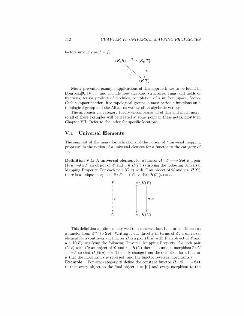
112 CHAPTER V. UNIVERSAL MAPPING PROPERTIES
factors uniquely as f = f0u.
(E,S) (F0, T )u //(E,S)
(F, T )
f
""DDDDDDDDDDD(F0, T )
(F, T )
f0
Nicely presented example applications of this approach are to be found inBourbaki[9, IV.3.] and include free algebraic structures, rings and fields offractions, tensor product of modules, completion of a uniform space, Stone-Cech compactification, free topological groups, almost periodic functions on atopological group and the Albanese variety of an algebraic variety.
The approach via category theory encompasses all of this and much more,so all of these examples will be treated at some point in these notes, mostly inChapter VII. Refer to the index for specific locations
V.1 Universal Elements
The simplest of the many formalizations of the notion of “universal mappingproperty” is the notion of a universal element for a functor to the category ofsets.
Definition V.1: A universal element for a functor H : C // Set is a pair(F, u) with F an object of C and u ∈ H(F ) satisfying the following UniversalMapping Property: For each pair (C, c) with C an object of C and c ∈ H(C)there is a unique morphism c : F // C so that H(c)(u) = c.
F
C
c
u
c
_
∈
∈
∈
∈
H(F )
H(C)
H(c)
This definition applies equally well to a contravariant functor considered asa functor from C op to Set. Writing it out directly in terms of C , a universalelement for a contravariant functor H is a pair (F, u) with F an object of C andu ∈ H(F ) satisfying the following Universal Mapping Property: for each pair(C, c) with Cq an object of C and c ∈ H(C) there is a unique morphism c : C
// F so that H(c)(u) = c. The only change from the definition for a functoris that the morphism c is reversed (and the functor reverses morphisms.)Example: For any category C define the constant functor H : C // Setto take every object to the final object 1 = 0 and every morphism to the

V.1. UNIVERSAL ELEMENTS 113
unique function from 1 to itself. Then H has a universal element iff C has aninitial object,and the universal element consists of the initial object and theunique element in one point set.
Equally well we have the constant contravariant functor H : C op // Set,and it has a universal element iff C has a final object with the object in theuniversal element being the final object.
Compare this discussion with the original discussion of the universal map-ping properties of initial (37) and final (37) objects.Example: The first example of a universal mapping property was for prod-ucts, and that fits here very well. Fixing C1 and C2, two objects of the categoryC , define the functor H : C // Set on an object C by H(C) = (f1, f2) :f1 : C1
// C,∧f2 : C2// C and on a morphism f : C // D by
H(f)(f1, f2) = (ff1, ff2). (The easy verification that H is a functor is left tothe reader.) Then a universal element for H consists of an object C1×C2 of Cand an element (π1, π2) ∈ H(C1 × C2) such that for every object C of C andevery (f1, f2) ∈ H(C) there is a unique morphism 〈f1, f2〉 : C1 × C2
// C(using the notation for products) with H(〈f1, f2〉)(π1, π2) = (f1, f2). Of coursethis is just another way of writing that 〈f1, f2〉 is the unique morphism suchthat π1〈f1, f2〉 = f1 and π2〈f1, f2〉 = f2. We summarize thus by saying thata product of C1 and C2 is a universal element for the functor H. This againemphasizes very well that a product of two objects is not just an object.
Sums fit here equally well. For fixed objects C1 and C2 there is the con-travariant functor K : C // Set defined by K(C) = (f1, f2) : f1 : C
// C1,∧f2 : C // C2 and on a morphism f : D // C by H(f)(f1, f2) =(f1f, f2f). Then a universal element for K consists of an object C1 + C2 andan element (ι1, ι2) ∈ K(C1 + C2) such that for every object C of C and every(f1, f2) ∈ K(C) there is a unique morphism [f1, f2] : C // C1 + C2 (us-ing the notation for sums) with H([f1, f2])(ι1, ι2) = (f1, f2). Of course thisis just another way of writing that [f1, f2] is the unique morphism such that[f1, f2]ι1 = f1 and [f1, f2]ι2 = f2. We summarize that by saying that a sumof C1 and C2 is a universal element for the functor K. This again emphasizesvery well that a sum of two objects is not just an object.Example: The other early example of a universal mapping property wasthe free monoid (see 87.) It fits here by taking a fixed set A and definingthe functor H : Monoid // Set on a monoid M to be H(M) = f : A
// U(M) and on a homomorphism h : M // N to be H(h)(f) = fU(h).(Here U is the forgetful functor from Monoid to Set. Again verification thatH is indeed a functor is left to the reader.) Now a universal element for His a monoid A∗ and an element of H(A∗), i.e., a function ε : A // U(A∗)such that every monoid M and each function f : A // U(M) there is aunique monoid homomorphism f∗ : A∗ // M extending f , i.e., the universalmapping property of the free monoid generated by A.
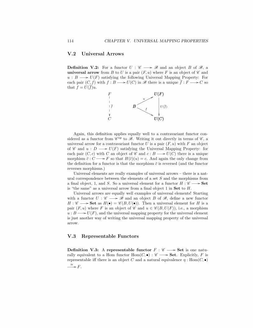
114 CHAPTER V. UNIVERSAL MAPPING PROPERTIES
V.2 Universal Arrows
Definition V.2: For a functor U : C // B and an object B of B, auniversal arrow from B to U is a pair (F, u) where F is an object of C andu : B // U(F ) satisfying the following Universal Mapping Property: Foreach pair (C, f) with f : B // U(C) in B there is a unique f : F // C sothat f = U(f)u.
F
C
f
B
U(F )u
77ooooooooo
U(F )
U(C)
U(f)
B
U(C)
f
''OOOOOOOOO
Again, this definition applies equally well to a contravariant functor con-sidered as a functor from C op to B. Writing it out directly in terms of C , auniversal arrow for a contravariant functor U is a pair (F, u) with F an objectof C and u : D // U(F ) satisfying the Universal Mapping Property: foreach pair (C, c) with C an object of C and c : B // U(C) there is a uniquemorphism c : C // F so that H(c)(u) = c. And again the only change fromthe definition for a functor is that the morphism c is reversed (and the functorreverses morphisms.)
Universal elements are really examples of universal arrows – there is a nat-ural correspondence between the elements of a set S and the morphisms froma final object, 1, and S. So a universal element for a functor H : C // Setis “the same” as a universal arrow from a final object 1 in Set to H.
Universal arrows are equally well examples of universal elements! Startingwith a functor U : C // B and an object B of B, define a new functorH : C // Set as H(•) = C (B,U(•)). Then a universal element for H is apair (F, u) where F is an object of C and u ∈ C (B,U(F )), i.e., a morphismu : B // U(F ), and the universal mapping property for the universal elementis just another way of writing the universal mapping property of the universalarrow.
V.3 Representable Functors
Definition V.3: A representable functor F : C // Set is one natu-rally equivalent to a Hom functor Hom(C, •) : C // Set. Explicitly, F isrepresentable iff there is an object C and a natural equivalence η : Hom(C, •)∼= // F .

V.4. INITIAL AND FINAL OBJECTS 115
Proposition V.14 The functor F : C // Set is representable iff it has auniversal element. If (U, u) is a universal element for F , then
η : Hom(U, •)∼= // F
is defined by ηC(f) = f∗(u). And if
η : Hom(U, •)∼= // F
is a natural isomorphism, then (U, ηU (1U )) is a universal element for F .
Proof: With (U, u) a universal element for F we verify that ηC(f) = f∗(u)does indeed define a natural transformation, i.e., that for any g : C // Dthis square commutes:
Hom(U,D) F (D)ηD//
Hom(U,C)
Hom(U,D)
g∗
Hom(U,C) F (C)ηC // F (C)
F (D)
F (g)
Which, for each f ∈ Hom(U,C), requires
F (g)ηC(f) = F (g)F (f)(u)= F (gf)(u)= ηD(gf)= ηD(g∗(f))= ηDg∗(f)
Going the other way, to show that for each object C and each c ∈ F (C),there is f : U // C with f(u) = c it suffices to show that for each morphismc ∈ Hom(U,C) ∼= F (C) there is an f with f∗(1U ) = c, and for that we can takef = c.
V.4 Initial and Final Objects
We’ve exhibited initial and final objects as universal elements, but we canequally well see that universal arrows are special cases of initial and final ob-jects! Given the datum for a universal arrow, i.e., a functor U : C // B andan object B of B, we have the comma category (see Section IV.1) (B ↓ U)which has as objects the pairs (C, f : B // U(C)) while a morphism from(C, f : B // U(C)) to (C ′, f ′ : B // U(C ′)) is a morphism g : C // C ′

116 CHAPTER V. UNIVERSAL MAPPING PROPERTIES
in C so that
B
U(C)f
77ooooooooo
U(C)
U(C ′)
U(g)
B
U(C ′)
f ′
''OOOOOOOOO
commutes.In this category an initial object is an object (F, u : B // U(F )) where
for any other object (C, f : B // U(C)) there is a unique morphism f : F// C in C so that
B
U(F )u
77ooooooooo
U(F )
U(C)
U(f)
B
U(C)
f
''OOOOOOOOO
commutes. And that is exactly the definition of a universal arrow from B toU . It is worthwhile to summarize this in a proposition.
Proposition V.15 Let U be a functor from C to Band B an object of B, thena universal arrow from B to U is an initial object of (B ↓ U), and conversely.
V.4.1 Free Objects
As mentioned above the motivating source of the name “universal mappings”was the notion of free structures in algebra. The context of based categoriesseems to give the best home for this notion. So let U : C // B be a categorybased on B and B and object of B.
Definition V.4: A free object in C generated by an object B of B is anobject F of C together with a morphism ι : B // U(F ) in B satisfyingthe following Universal Mapping Property: For every object C in C and everymorphism f : B // U(C) there is a unique morphism f : F // C
F
C
f
B
U(F )ι
77ooooooooo
U(F )
U(C)
U(f)
B
U(C)
f
''OOOOOOOOO

V.5. LIMITS AND COLIMITS 117
V.5 Limits and Colimits
The most familiar and widely used universal mapping properties are limits andcolimits. Our very first examples of limits and colimits were products andcoproducts, with initial and final objects close behind. As with these, otherlimits and colimits are most immediately associated with the internal structureof a category. But the preservation and creation of limits is also an importantstructural property of functors.
In various guises, and with various names, limits (and colimits) well predatethe introduction of categories and functors. In most cases the universal map-ping property was not made explicit, often because it was essentially trivial.For example the null space of a linear transformation has the following univer-sal mapping property: For any linear transformation L : V // W betweentwo vector spaces over a field K there is the inclusion N(L) → V of the nullspace of L, i.e., the subspace of V consisting of all vectors v with L(v) = 0. IfK : U // V is any other linear transformation with LK = 0, then there is aunique linear transformation K : U // N(L) such that the following diagramcommutes:
V WL
//
N(L)
V
N(L) 00 // 0
W
0
U
0
0
''OOOOOOOOOOOOOOOOOOOOU
N(L)
K
??
??
U
V
K
////////////////////
This is representative of a number of similar situations. For example Lmight be a group homomorphism whereupon we similarly have the kernel of L,a normal subgroup, in place of N(L). In the category of sets the situation ismore complicated as there is no direct analog of the kernel for functions, butrather the equivalence relation
E = (x1, x2) : x1, x2 ∈ X with f(x1) = f(x2)
defined by the function (see exercise I.31 on page 22.) Here for any pair offunctions g1, g2 : Z // X with fg1 = fg2 there is a unique function g : Z
// E such that g1 = π1g and g2 = π2g. This is summarized in the following

118 CHAPTER V. UNIVERSAL MAPPING PROPERTIES
commutative diagram.
X Yf
//
E
X
π2
E Xπ1 // X
Y
f
Z
X
g1
''OOOOOOOOOOOOOOOOOOOOZ
E
g?
??
??
?
Z
X
g2
////////////////////
Another similar construction occurs when discussing fiber spaces in topol-ogy. A fiber space is a continuous surjection p : E // B. (Of course E andB must be topological spaces, and there are usually additional conditions thatare imposed such as requiring that E is “locally a product”.) If f : A // B isany continuous function, then there is a pullback of p along f which is a fiberspace p : f∗E // A with the universal mapping property captured in thefollowing commutative diagram:
A Bf
//
f∗E
A
p
f∗E Ef // E
B
p
X
E
gE
**TTTTTTTTTTTTTTTTTTTTTTTTTTTTTX
f∗E
g?
??
??
?
X
A
gA
////////////////////
This last universal mapping property is suitable and sufficiently importantto state in an arbitrary category.
Definition V.5: Given morphisms f : A // C and g : B // C, a pullbackof f and g is a pair of morphisms πA : A×C B // A and πB : A×C B // Bsatisfying the universal mapping property:
A Cf
//
A×C B
A
πA
A×C B BπB // B
C
g
D
B
k
''OOOOOOOOOOOOOOOOOOOOD
A×C B
<h,k>
??
??
D
A
h
////////////////////

V.5. LIMITS AND COLIMITS 119
This is indeed a generalization of the previous examples – they are all specialcases for suitably chosen categories and morphisms.
Just as with products and final objects and universal mapping objects ingeneral, pullbacks need not exist, but when they do they are unique up toa unique isomorphism. The statement and proof of this result for arbitrarylimits, not just pullbacks, is in Proposition V.16.
Exercise V.1. Verify that pullbacks always exist in Set. For functionsf : A // C and g : B // C, define
A×C B = (a, b) : a ∈ A, b ∈ B ∧ f(a) = g(b) ⊆ A×B
and define the two projection functions to be the restrictions of the projectionson A×B, then show that this has the requisite universal mapping property.
Products, final objects and all the versions of pullbacks are examples oflimits. Just as for products and final objects there are the dual notions ofcoproducts and initial objects, there is a dual to the notion of pullbacks. Theseare called pushouts and are a fundamental examples of colimits. We could justsay that a pushout is a pullback in the dual category, but it is worthwhile tospell out the definition explicitly in the category itself.
Definition V.6: Given morphisms f : C // A and g : C // B, a pushoutof f and g is a pair of morphisms ιA : A // A+C B and ιB : B // A+C Bsatisfying the universal mapping property:
A Coof
A+C B
A
OO
ιA
A+C B Boo ιB B
C
OO
g
D
B
gg
k
OOOOOOOOOOOOOOOOOOOOD
A+C B
__
[h,k]
??
??
D
A
WW
h
////////////////////
So again pushouts need not exist, but when they do they are unique up toa unique isomorphism.
Various familiar constructions in various parts of mathematics are examplesof pushouts. For any linear transformation L : V // W between two vectorspaces over a field K there is the cokernel of L which is W/Im(L). This is the

120 CHAPTER V. UNIVERSAL MAPPING PROPERTIES
pushout of L and 0 as shown here.
0 Voo0
Coker(L)
0
OO
0
Coker(L) Woo QW
V
OO
L
U
W
jj
K
TTTTTTTTTTTTTTTTTTTTTTTTTTTTTU
Coker(L)
__
K
??
??
U
0
WW
0
////////////////////
The universal mapping property here is “KL = 0 implies there exists a uniquelinear transformation K with K = KQ”.
Just as with pullbacks, this is representative of a number of similar situa-tions. For example L might be a group homomorphism whereupon we similarlyhave the cokernel of L, which is the quotient of W by the normal subgroupgenerated by the image of L in place of N(L).
In the category of sets the situation is considerably less familiar, just ascoproducts of sets are less familiar than products. Also there is no directanalog of the cokernel for functions, rather for f : X // Y there is the“amalgamated sum” Y +X Y which is the quotient of the disjoint union of Ywith itself (Y + Y ) by the equivalence relation that identifies elements comingfrom a common element of X. In detail,
Y + Y = (yi, i) : i ∈ 0, 1 ∧ yi ∈ Y
(see definition I.35) and Y +X Y is (Y + Y )/ ∼ where ∼ is the equivalencerelation generated by the requirement that (f(x), 0) ∼ (f(x), 1) for all x ∈ X(see the discussion on page 192.)
Here for any pair of functions g0, g1 : Y // Z with g0f = g1f there is aunique function g : Y +X Y // Z such that g0 = gι0 and g1 = gι1. This issummarized in the following commutative diagram.
Y Xoof
Y +X Y
Y
OO
ι1
Y +X Y Yoo ι0Y
X
OO
f
Z
Y
jj
g0
TTTTTTTTTTTTTTTTTTTTTTTTTTTTTZ
Y +X Y
__
g?
??
??
?
Z
Y
WW
g1
////////////////////
This construction is most commonly used in topology under the name “ad-junction space”. When X and Y are topological spaces, A is a subspace of Y

V.5. LIMITS AND COLIMITS 121
(with the inclusion function ι : A → Y ) and f : A // X is a continuous func-tion (which is called the attaching map.) Then the pushout X +A Y is calledan adjunction space and is constructed by taking the disjoint union of X andY modulo the equivalence relation generated by requiring that a is equivalentto f(a) for all a ∈ A. Intuitively we think of the spaces X and Y being gluedtogether along the subspace A, with the function f providing the glue.
A simple and important example arises when X and Y are each a closeddisk, A is the bounding circle and f is the inclusion. Then the adjunctionspace is (homeomorphic to) the 2-sphere. This works equally well when Xand Y are both closed n-balls (or n-cells) and A is the bounding n-1-sphere togive the (n+1)-sphere. Iteratively attaching cells of various dimensions leadsto the definition of CW-complexes, an important class of spaces much used inalgebraic topology. For information on CW-complexes look at Lundell [48] orHatcher [30].
V.5.1 Cones and Limits
All of the examples take the form of some common “diagram” of objects andmorphisms from the category C and then considering an object with a univer-sal family of mappings into the diagram. A number of different ways have beendeveloped for specifying what is meant by a suitable diagram, using graphs, di-agram schemes, free categories and, the method used here, arbitrary categories.(For discussions of the various approaches see Barr and Wells [3], Popescu andPopescu [63], and Mac Lane [54].)
For any small category D and arbitrary category C we have the diagonalfunctor ∆ : C // C D which on objects has ∆(C) = C, the constant functorselecting C, and on morphisms just selects the corresponding natural transfor-mation between the relevant constant functors. For any functor F : D // Cwe also have the constant functor 1 // C D which selects F , and from thesewe can form the comma category (∆ ↓ F ). It is helpful to describe the objectsand morphisms somewhat more concretely. From the general definition, anobject (C, φ : C // F, 1) in (∆ ↓ F ) consists of an object C from C and theunique object 1 in 1 together with a natural transformation φ from the con-stant functor selecting C to the functor F . The object 1 being unvarying, thisis the same as saying an object C together with a natural transformation φ : C
// F . And this is, for each object D in D, a morphism φD : C // F (D)(in C ) such that for every morphism f : D // D′ of D the diagram
F (D) F (D′)F (f)
//
C
F (D)
φD
C
F (D′)
φD′
???????????
is commutative.

122 CHAPTER V. UNIVERSAL MAPPING PROPERTIES
Definition V.7: Let F : D // C be a functor. A cone over F is an objectC of C and a natural transformation φ : C // F from the constant functorC to F . This is the same as saying that for every morphism f : D // D′ ofD the triangle
F (D) F (D′)F (f)
//
C
F (D)
φD
C
F (D′)
φD′
???????????
commutes.A morphism from the cone (C, φ) to the cone (C ′, φ′) is a morphism f : C// C ′ with φ′f = φ. (NB the morphism f : C // C ′ can be considered
equally well as a morphism in C and as a natural transformation between thetwo constant functors.)
Clearly there is a category of cones over F with objects and morphism asin the preceding definition. We write this category as C /F .
When the category D is very small a functor can be conveniently specifiedby giving the objects and morphisms that are the values of the functor. Forexample we will speak of “a pair of morphisms” instead of talking about “thefunctor that maps the two non-trivial morphisms in D to the pair of morphismsof interest”. We will be equally casual when we actually need to talk aboutthat category D and just describe it as
• •//• •//
This category has four distinct objects with the corresponding four identitymorphisms, the two morphisms indicated and no other morphisms.
This is all preliminary to giving the actual definition of a limit.
Definition V.8: Let F : D // C be a functor. A limit for F is a finalobject (L, φ) in C /F . This is also called a universal cone over F and is a coneφ : L // F with the universal mapping property that for any cone ψ : N
// F there is a unique morphism u : N // L such that for every object Dof D φDou = ψD. Explicitly, this says for for every morphism f : D1
// D2

V.5. LIMITS AND COLIMITS 123
in D this diagram is commutative:
F (D1) F (D2)F (f)
//
N
F (D1)
ψD1
N
F (D2)
ψD2
////////////////////N
L
u
F (D1) F (D2)F (f)
//
L
F (D1)
φD1
L
F (D2)
φD2
???????????
As with all universal mapping objects limits are essentially unique.
Proposition V.16 Let F : D // C be a functor. If φ : L // F and φ′ : L′// F are both limits of F , then there is a unique isomorphism u : L // L′
such that φ′u = φ.
Proof: The proof is much the same as every other uniqueness proof foruniversal mapping properties. As L′ is a limit of F and φ is a cone over Fthere is a unique morphism u : L′ // L such that φ′u = φ. And as L is alimit of F and φ′ is a cone over F there is a unique morphism v : L′ // Lsuch that φv = φ′. Next we note that φ′uv = φv = φ′ whence uv must be1L as that is the unique morphism which composed with φ gives φ. Finally asφvu = φ′u = φ we equally well conclude that vu = 1L′ .
As with other universal mapping objects we will use this to justify referringto the limit of the functor F , and we will write lim←−F for the object of thecone over F that is its limit. For each object D of D we will write πD : lim←−F
// F (D) for the component of the natural transformation π : lim←−F// F
that is the remaining part of the limit.Examples
1. Final Object
The 0 empty category is the initial category, i.e., there is a unique(empty!) functor from 0 to any other category C . A cone over theempty functor is nothing but an object of C as a natural transformationfrom C to that empty functor is vacuous. So a universal cone in this caseis just an object 1 where there is a unique morphism from every objectto 1, i.e., a final object in C .
2. Initial Object
Curiously initial objects are also limits in an even more extreme manner,as the limit of the identity functor 1C .

124 CHAPTER V. UNIVERSAL MAPPING PROPERTIES
Proposition V.17 If lim←−1C exists in C , then lim←−1C is an initial objectin C , and if C has an initial object then it is a limit for 1C .
Proof: Recall that a cone over the identity functor 1C is a naturaltransformation ψ : D // 1C from some constant functor D selectingthe corresponding object in C . This is a family of morphisms ψC : D
// C having the property that for every morphism f : C // C ′ thetriangle
C C ′f
//
D
C
φC
D
C ′
φC′
???????????
commutes. A limit for 1C is a universal cone (L, φ) which is final inC /1C . Consider in particular the triangle
L CφC
//
L
L
φL
L
C
φC
???????????
For every object C this commutes just because φ is a cone over 1C . Butthis says that φφL is not only a cone over 1C but is the same cone as φfrom which we conclude that φL must be 1L. Now considering
L Cf
//
L
L
φL
L
C
φC
???????????
with f an arbitrary morphism from L to C we see that φC = fφL = f asφL = 1L. So for each object C there is exactly one morphism (φC) fromL to C which is just what it means for L to be an initial object of C .
For the other direction, if 0 is an initial object of C , then we certainlyhave a cone over 1C given by ! : 0 // 1C with !C being the uniquemorphism from 0 to C. We also see that !0 must be 10 as there is exactlyone morphism from 0 to 0.
Now suppose ψ : D // 1C is a cone over 1C , then in particular we haveψ0 : D // 0 which is a cone morphism from ψ to !, i.e., the following

V.5. LIMITS AND COLIMITS 125
diagram commutes:
C C ′C C ′
D
C
ψC
D
C ′
ψC′
////////////////////D
0
ψ0
C C ′C C ′
0
C
!C
0
C ′
!C′
???????????
In order to show that 0 is the limit of 1C we have to verify that ψ0 is theunique such morphism. But if g : D // 0 is such a morphism then inparticular we have ψ0 =!0g = g.
3. Product
When D is a finite discrete category with objects 1, · · · , n, a functor fromD to C simply selects n objects C1, · · · , Cn. A cone over the functorselecting (C1, · · · , Cn) is just a family of morphisms fi : C // Ci anda limit (universal cone) is an object Πn
i=1Ci and a family of morphismsπ1, · · · , πn satisfying the universal mapping property that for any familyof morphisms fi : C // Ci there exists a unique morphism 〈f1, · · · , fn〉 :C // Πn
i=1Ci with πi〈f1, · · · , fn〉 = fi.
C Πni=1Ci
〈f1,··· ,fn〉 //________C
Ci
fi
''OOOOOOOOOOOOOOOOOOO Πni=1Ci
Ci
πi
Of course as advertised this is exactly the universal mapping property forthe product of C1, · · · , Cn in C .
The empty category is actually the discrete category with zero objects,so this is yet again reinforcing the remark that the final object is just theempty product!
While the above discussion assumed that D was a finite discrete category,that was relevant only to connecting the limit of a functor from D to Cwith the prior discussion of products. This allows us to define the productof an arbitrary family of objects in C to be the limit of a functor fromsome discrete category which selects those objects. From this point on

126 CHAPTER V. UNIVERSAL MAPPING PROPERTIES
we will freely use diagrams such as the following:
C Πi∈DCi〈fi:i∈D〉 //________C
Cj
fj
''OOOOOOOOOOOOOOOOOOO Πi∈DCi
Cj
πj
Of course just because we can define products of arbitrary families ofobjects, that says noting about existence of such product. In particularwhile assuming all products of two objects exists guarantees that all finiteproducts exists, it says nothing about existence of products of infinitefamilies. This will be discussed further in section V.5.3
Proposition V.18 Suppose that in the category C all products exist,i.e., for every functor F : D // C with D any discrete category, theproduct lim←−F exists, then C is preordered.
Proof: Suppose that f, g : B // C in C , and consider product P =ΠDC where D is a proper class. For each D in D take fD : B // P tobe the unique morphism such that πDfD = f and πD′fD = g for D′ 6= D.If g is not equal to f , then each of the fD is distinct and so Hom(B,P )is a proper class contrary to the definition of a category. Whence weconclude that any parallel morphisms are equal, which is the definitionof a preordered category!
4. Kernel
Whenever C is a category with a zero object, we can define the kernel ofa morphism.
Definition V.9: A kernel of f : C // D is a morphism k : K // Cwith
a) fk = 0, and
b) If g is any morphism with fg = 0, then there is a unique morphismg so that g = kg.
As always with universal mapping properties the item of interest is themorphism k (which determines K), but it is K which is named as Ker(f).Following the usual practice we will often write of “the kernel Ker(f)of f”, but it must be understood that this tacitly includes the specificmorphism k : Ker(f) // C. Of course the reason for this is that inthe most familiar categories the kernel of a morphism is a subset of thedomain and the morphism k is just the inclusion

V.5. LIMITS AND COLIMITS 127
In general a morphism may not have a kernel, but if it does it is uniquein the strong sense that when k : K // C and k′ : K ′ // C are twokernels of f : C // D, there is a unique isomorphism k : K // K ′
with k′k = k. The inverse being k′ : K ′ // K.
An easy but important observation is that every kernel is a monomor-phism.
Proposition V.19 In any category with zero object, if k : Ker(f) // Cis a kernel, then it is a monomorphism.
Proof: Suppose g1 and g2 are morphisms to Ker(f) and kg1 = kg2. Thenfkg1 and fkg2 are both zero morphisms, so there is a unique morphismg so that kg = kg1. But both g1 and g2 have that property so they mustbe equal.
While every kernel is a monomorphism, the converse is not true.
Exercise V.2. Give an example of a monomorphism that is not a kernel.(Hint: Consider the inclusion of N into Z in the category of monoids.)
We’ve previously noted that the category theory notion of monomor-phism does not capture all the meaning associated with injective homo-morphisms. This is part of that and leads to the following definitions.
Definition V.10: In a category with zero, a normal monomorphismis a morphism that is the kernel of some morphism.
Definition V.11: A normal category is a category with zero in whichevery monomorphism is normal.
The most familiar examples of normal categories are the categories ofmodules, including the category of Abelian groups and the category ofvector spaces over a particular field. These are all example of Abeliancategories and will be discussed at length in Chapter XIII.
Examples of kernels abound. In the category of groups there is the usualnotion of the kernel of a group homomorphism h : G // G′, namelyKer(h) = g ∈ G : h(g) = 1 where 1 is the identity element in G′. Thenthe inclusion morphism i : Ker(h) // G is a kernel of h according tothe above definition.
Similarly in the category of modules over a particular ring there is againthe usual notion of the kernel of a module homomorphism h : M // M ′
as Ker(h) = m ∈ M : h(m) = 0 where 0 is the zero element in M ′.Again the inclusion morphism i : Ker(h) // M is a kernel of h as above.

128 CHAPTER V. UNIVERSAL MAPPING PROPERTIES
This last includes kernels for homomorphisms of Abelian groups (Z-modules) and null spaces for linear transformations (K-modules for thebase field K.) At the same time it is really a special case of the kernelof a group homomorphism as all that is being used here is the kernel ofthe module homomorphism considered as a homomorphism of (Abelian)groups. In Chapter XIII on Abelian Categories, we will see that in acertain sense these are all the interesting cases, but we will also see thevalue of the abstraction.
A more general case is the category of monoids. Again conventionally thekernel of a monoid homomorphism h : M // M ′ is Ker(h) = m ∈M :h(m) = 1 where 1 is the identity element in M ′. Again the inclusionmorphism i : Ker(h) // M is a kernel of h as above. This includes thekernel of group homomorphisms as a special case, but we will see laterthat this illustrates that the notion of a kernel is only useful in specialcases.
There are numerous other cases in algebra where it is common to speakof kernels that are not captured by this definition. For example inthe category of commutative rings it is usual to define the kernel of aring homomorphism f : R // S as Ker(f) = r ∈ R : f(r) = 0.But this is an ideal of R rather than a subring. Indeed the categoryCommutativeRing has no zero object (as the rings in CommutativeRingall have 1 different from 0), so the definition of a kernel given in this sec-tion simply does not apply.
5. Equalizer
Kernels are specializations of the more general notion of equalizers whichconcerns two morphisms between the same objects.
Definition V.12: Two morphisms are parallel if they have the samedomain and the same codomain. This is usually written symbolically as
•f //g
// • or justf //g
//.
Definition V.13: An equalizer of parallel morphisms f and g is amorphism k with
a) fk = gk, and
b) If h is any morphism with fh = gh, then there is a unique morphismh so that h = kh.
Kernels are special cases of equalizers where one of the two parallel mor-phisms is a zero morphism. Just as with kernels, equalizers need notexist, but if they do exists any two equalizers of the same parallel pair

V.5. LIMITS AND COLIMITS 129
are isomorphic via the unique morphisms between guaranteed by the def-inition.
Besides the examples of kernels, equalizers also arise in the category ofsets and related categories. In Set if f, g : X // Y are two parallelfunctions, then taking K // x ∈ X : f(x) = g(x) and k : K //
X the inclusion function exhibits k as an equalizer of f and g. Thissame construction serves in the category Top of topological spaces andcontinuous maps where K is simply considered as a subspace of X.
Equalizers are also called difference kernels because in certain situationsthey arise as the kernel of the difference of two morphisms. For examplein all categories of modules the Hom-set natural structure of an Abeliangroup, so for any pair of morphisms f, g : M // N there is the mor-phism f − g : M // N with f − g(m) = f(m)− g(m). And in this casethe kernel of f − g is an equalizer of f and g. This situation prevails inall preadditive categories as will be discussed in Chapter XIII.
Just as every kernel is a monomorphism, so is every equalizer and withessentially the same proof. Suppose that k : K // C is an equalizerof f, g : C // D and h1, h2 are morphisms to Ker(f) with kh1 = kh2.Then fkh1 = gkh1, so there is a unique morphism h so that kh = kh1.But both h1 and h2 have that property so they must be equal.
6. Pullback
Pullbacks were defined back on page 118 as examples of limits, and hereis that remark made precise. When D is the category
• •// •
•
a functor F from D to C selects three objects A, B and C in C togetherwith two morphisms f : A // C and g : B // C, i.e., the diagram
A Cf // C
B
g
and the limit of F is exactly the pullback of f and g as previously defined.
Equalizers are just pullbacks where the morphisms are parallel, i.e., theyhave the same domain as well as the same codomain.
In the category of sets the canonical pullback of f and g is the subset
A×C B = (a, b) ∈ A×Bsuchthatf(a) = g(b),

130 CHAPTER V. UNIVERSAL MAPPING PROPERTIES
of A×B together with the restrictions of the projection maps π1 and π2
to A×C B .
This example motivates another way of characterizing the pullback: asthe equalizer of the morphisms fπ1, gπ2 : A× CB
// // C.
Exercise V.3. Verify that in any category with finite products, pullbacks andequalizers, the pullback of f : A // C and g : B // C is the equalizer offπ1 and gπ2.
This shows that pullbacks exist in any category with binary products andequalizers.
Clearly in any category with a terminal object 1, the pullback A× 1B isjust the product A×B.
Every square
Y Zg//
P
Y
q
P Xp // X
Z
f
where (P, p, q) is a pullback of (f, g) is called a Cartesian square.
Proposition V.20 Any morphism f : X // Y is a monomorphism iff thecommutative square
X Yf
//
X
X
1X
X X1X // X
Y
f
is Cartesian.
V.5.2 Cocones and Colimits
Everything in the previous section has a dual, but these dual notions are suffi-ciently common and important that this section provides all of the definitionsand results explicitly, though the proofs follow from the dual results so nothingfurther need be said.
The dual of a cone is a cocone, again a family of commuting triangles butnow pointing down.
Definition V.14: Let F : D // C be a functor. A cocone over F isan object C of C and a natural transformation φ : F // C from F to the

V.5. LIMITS AND COLIMITS 131
constant functor C. This is the same as saying that for every morphism f : D// D′ of D this triangle commutes:
F (D)
C
φD??????????
F (D) F (D′)F (f) // F (D′)
C
φD′
A morphism from the cocone (C, φ) to the cocone (C ′, φ′) is a morphismf : C // C ′ with φf = φ′.
Clearly there is a category of cocones over F with objects and morphismas in the preceding definition. We will denote this category by F/C .
Dual to the notion of a limit is a colimit which is a universal cocone just asa limit is a universal cocone..
Definition V.15: Let F : D // C be a functor. A colimit for F is aninitial object (C, φ) in F/C . This is also called a universal cocone over F andis a cocone φ : F // C with the universal mapping property that for anycocone ψ : F // B there is a unique morphism u : C // B so uφ = ψ.Explicitly, this says for for every morphism f : D // D′ in D this diagram iscommutative:
F (D)
C
φD
''OOOOOOOOOOOOOOOOOOF (D) F (D′)F (f) // F (D′)
C
φD′
wwoooooooooooooooooo
C
B
u
F (D)
B
ψD
????????????????????????F (D′)
B
ψD′
Proposition V.21 Let F : D // C be a functor. If φ : F // C and ψ : F// B are both colimits of F , then there is a unique isomorphism u : B // C
such that uφ = ψ.
As with other universal mapping objects we will use this to justify referringto the colimit of the functor F , and we will write lim−→F for the object of thecocone over F that is its limit. We will write ι : F // lim−→F for the naturaltransformation that is the remaining part of the colimit.
Examples

132 CHAPTER V. UNIVERSAL MAPPING PROPERTIES
1. Initial Object
The 0 empty category is the initial category, i.e., there is a unique(empty!) functor from 0 to any other category C . A cocone over theempty functor is nothing but an object of C as a natural transformationfrom C to that empty functor is vacuous. So a universal cocone in thiscase is just an object 0 where there is a unique morphism from everyobject to 0, i.e., an initial object in C .
2. Final Object
A final objects is the colimit of the identity functor 1C , and conversely.
Proposition V.22 If lim−→1C exists in C , then lim−→1C is a final object inC , and if C has a final object 1 then it is the colimit of 1C .
3. Sum
Sums are the duals of products, and they occur as colimits of functors ondiscrete categories.
When D is a finite discrete category with objects 1, 2, · · · , n, a functorfrom D to C simply selects n objects C1, . . . , Cn. A cocone over thefunctor selecting (C1, · · · , Cn) is just a family of morphisms fi : Ci // Cand a colimit (universal cocone) is an object Σni=1Ci and a family ofmorphisms ι1, · · · , ιn satisfying the universal mapping property that forany family of morphisms fi : Ci // C there exists a unique morphism[f1, · · · , fn] : Σni=1Ci
// C with [f1, · · · , fn]ιi = fi.
C Σni=1Cioo [f1,··· ,fn] ________C
Ci
gg
fi
OOOOOOOOOOOOOOOOOOO Σni=1Ci
Ci
OO
ιi
Of course as advertised this is exactly the universal mapping property forthe sum of C1, · · · , Cn in C .
The empty category is actually the discrete category with zero objects,so this is yet again reinforcing the remark that the initial object is justthe empty sum!
While the above discussion assumed that D was a finite discrete category,that was relevant only to connecting the colimit of a functor from D toC with the prior discussion of sums. This allows us to define the sum ofan arbitrary family of objects in C to be the colimit of a functor fromsome discrete category which selects those objects. From this point on

V.5. LIMITS AND COLIMITS 133
we will freely use diagrams such as the following:
C Σi∈DCioo [fi:i∈D] ________C
Cj
gg
fj
OOOOOOOOOOOOOOOOOOO Σi∈DCi
Cj
OO
ιj
Of course just because we can define sums of arbitrary families of objects,that says noting about existence of such product. In particular whileassuming all sums of two objects exists guarantees that all finite sumsexists, it says nothing about existence of sums of infinite families. Thiswill be discussed further in section V.5.3.
4. Cokernel
Dual to kernels are cokernels, and just as with kernels they can be definedin any category that has a zero object (a self-dual notion.)
Definition V.16: In a category with a zero object, a cokernel of f : E// D is a morphism c : D // C with
a) cf = 0, and
b) If g is any morphism with gf = 0, then there is a unique morphismg so that g = gc.
As always with universal mapping properties the item of interest is themorphism c (which determines C), but it is C which is named as Coker(f).Following the usual practice we will often speak of “the cokernel Coker(f)of f”, but it must be understood that this tacitly includes the specificmorphism c : D // Coker(f).
In general a morphism may not have a cokernel, but if it does it is uniquein the strong sense that when c : D // C and c′ : D // C ′ are twocokernels of f : E // D, there is a unique isomorphism c : C // C ′
with cc′ = c. The inverse being c′ : C ′ // C.
Of course just as every every kernel is a monomorphism, every cokernelis an epimorphism, a fact we record as a proposition.
Proposition V.23 In any category with zero object, if c : B // Coker(f)is a cokernel, then it is an epimorphism.
While every cokernel is an epimorphism, the converse is not true.
Exercise V.4. Give an example of an epimorphism that is not a cokernel.(Hint: Consider the inclusion of N into Z in the category of monoids.)

134 CHAPTER V. UNIVERSAL MAPPING PROPERTIES
We’ve previously noted that the category theory notion of epimorphismdoes not capture all the meaning associated with surjective homomor-phisms. This is part of that and leads to the following definitions.
Definition V.17: A morphism in a category with zero is a normalepimorphism provided it is the cokernel of some morphism.
Definition V.18: A conormal category is a category in which everyepimorphism is conormal.
The most familiar examples of conormal categories are all categories ofmodules, including the category of Abelian groups and the category ofvector spaces over a particular field. These are all example of Abeliancategories and will be discussed at length in Chapter XIII.
In the category of modules over a ring there is again the notion of thecokernel of a module homomorphism being the quotient of the codomainby the image. This includes cokernels for homomorphisms of Abeliangroups (Z-modules) and cokernel for linear transformations (K-modulesfor the base field K.) At the same time it is really a special case of thecokernel of a group homomorphism as all that is being used here is thecokernel of the module homomorphism considered as a homomorphismof (Abelian) groups. In Chapter XIII on Abelian Categories, we will seethat in a certain sense these are all the interesting cases.
5. Coequalizer
Cokernels are specializations of the more general notion of coequalizerswhich concerns two parallel morphisms.
Definition V.19: An coequalizer of parallel morphisms f and g is amorphism c with
a) cf = cg, and
b) If h is any morphism with hf = hg, then there is a unique morphismh so that h = hc.
Cokernels are special cases of equalizers where one of the two parallelmorphisms is a zero morphism. Just as with cokernels, equalizers neednot exist, but if they do exists any two coequalizers of the same parallelpair are isomorphic via the unique morphisms between guaranteed by thedefinition.
Coequalizers are also called difference cokernels because in certain situ-ations they arise as the kernel of the difference of two morphisms. For

V.5. LIMITS AND COLIMITS 135
example in all categories of modules the Hom-set is naturally an Abeliangroup, so for any pair of morphisms f, g : M // N there is the mor-phism f − g : M // N with f − g(m) = f(m)− g(m). And in this casethe cokernel of f − g is an coequalizer of f and g. This situation prevailsin all preadditive categories as will be discussed in Chapter XIII.
Just as every cokernel is an epimorphism, so is every coequalizer.
6. Pushout
Pushout are the duals of pullbacks and provide a good example of thevalue of alternative views of duality. The diagram category for a pullbackis
• •// •
•
so a pushout in the category C can be described as the limit of a functorfrom this diagram category to C op. But that diagram can equally wellbe considered as a functor from the dual of the diagram category to C ,and usually we consider the diagram category D
• •//•
•
and specific diagrams like
C Af //C
B
g
So the pushout A × CB of f and g is the colimit of the functor from Dto C that selects f and g.
By duality, exercise V.3 shows that in any category with finite sums andcoequalizers, the pushout A +C B of f : C // A and g : C // B isthe coequalizer of ι1f and ι2g.
This is the abstract justification of the construction of pushouts in Setgiven on page 119.
Dual to the results for pullbacks, this shows that pushouts exist in anycategory with binary sums and coequalizers, and that in a category withan initial object 0, the pushout X +0 Y is just the sum X + Y .

136 CHAPTER V. UNIVERSAL MAPPING PROPERTIES
Every square
X Zg//
Y
X
OO
f
Y Pi // P
Z
OO
j
where (P, p, q) is a pushout of (f, g) is called a coCartesian square.
Proposition V.24 Any morphism f : X // Y is an epimorphism iff thecommutative square
X Yf
//
Y
X
OO
f
Y Y1Y // Y
Y
OO
1Y
is coCartesian.
Of course this is the dual of proposition V.20, so no additional proof isneeded.
V.5.3 Complete Categories
Definition V.20: A category is complete if it has all small limits.
Theorem V.10 small products and kernels implies complete
Definition V.21: A category is cocomplete if it has all small colimits.
Theorem V.11 small sums and cokernels implies cocomplete
V.6 Adjoint Functors
“Adjoints are everywhere”
That slogan, useful for anyone studying categories, has already been re-inforced by the examples of adjoint functors provided in a number of earlierexercises. See exercises III.11, III.15, III.16, III.18, III.25, III.27, III.31, andIII.34.
No definition has been provided to this point, so this section will providethe definition, including a number of alternative formulations, and some basictheory about adjoint functors.

V.6. ADJOINT FUNCTORS 137
The basic context for adjoints consists of two functors U : M // S andF : S // M . [Throughout this section we will generally use these namesas they are intended to suggest the underlying and free functors between thecategory of modules (or monoids) and the category of sets.]
The basic definition is in terms of natural transformations ε : 1S// UF
and η : FU // 1M , while the memorable formulation is in terms of thebifunctors M (F (•), •) and S (•, U(•)) both from S op ×M to Set.
As bifunctors these are both functors from S op ×M to Set. So for eachpair of morphisms (f : T // S, h : M // N) we have the induced functionsM (F (f), h) and S (f, U(h)). This notation is so cumbersome that we willusually use the notation (F (f), h)∗ and (f, U(h))∗ in its place. Notice thatfor example (f, U(h))∗(g) = U(h)gf so that this is a direct extension of thenotation first introduced in definitions I.7 and I.8. In particular in the casethat f is an identity morphism, we will write h∗ instead of M (F (S), h) andU(h)∗ instead of S (S,U(h)). Similarly when h is an identity morphism, wewill write F (f)∗ instead of M (F (f),M) and f∗ instead of S (f, U(M)).
The first observation is that the natural transformations ε and η inducenatural transformations φ : M (F (•), •) // S (•, U(•)) and ψ : S (•, U(•))
// M (F (•), •) defined as follows.If s ∈ S (S,U(M)), then φS,M (s) = ηMF (s)
F (S) FU(M)F (s)//F (S)
M
φS,M (s)
??????????FU(M)
M
ηM
while for m ∈M (F (S),M), the definition is ψS,M (m) = U(m)ε
UF (S) U(M)U(m)//UF (S)
S
OO
εS
U(M)
S
??
ψS,M (m)
To verify that φ and ψ are natural transformations requires checking thatfor all morphisms t : T // S in S and n : M // N in M the following arecommutative squares.
M (F (T ), N) S (T,U(N))φT,N
//
M (F (S),M)
M (F (T ), N)
(F (t),n)∗
M (F (S),M) S (S,U(M))φS,M // S (S,U(M))
S (T,U(N))
(t,U(n))∗
S (T,U(N)) M (F (T ), N)
ψT,N
//
S (S,U(M))
S (T,U(N))
(t,U(n))∗
S (S,U(M)) M (F (S),M)ψS,M // M (F (S),M)
M (F (T ), N)
(F (t),n)∗
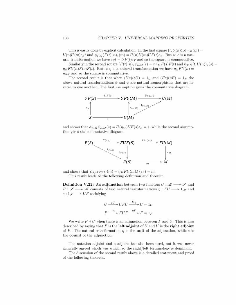
138 CHAPTER V. UNIVERSAL MAPPING PROPERTIES
This is easily done by explicit calculation. In the first square (t, U(n))∗φS,M (m) =U(n)U(m)εSt and φT,N (F (t), n)∗(m) = U(n)U(m)UF (t)εT . But as ε is a nat-ural transformation we have εSt = UF (t)εT and so the square is commutative.
Similarly in the second square (F (t), n)∗ψS,M (s) = nηMF (s)F (t) and ψT,N (t, U(n))∗(s) =ηNFU(n)F (s)F (t). But as η is a natural transformation we have ηNFU(n) =nηN and so the square is commutative.
The second result is that when (Uη)(εU) = 1U and (Fε)(ηF ) = 1F theabove natural transformations φ and ψ are natural isomorphisms that are in-verse to one another. The first assumption gives the commutative diagram
S U(M)s//
UF (S)
S
OO
εS
UF (S) UFU(M)UF (s) // UFU(M)
U(M)
OO
εU(M)
UFU(M) U(M)U(ηM ) //
U(M)
U(M)
1U(M)
77oooooooooooooooo
and shows that φS,MψS,M (s) = U(ηM )UF (s)εS = s, while the second assump-tion gives the commutative diagram
F (S) Mm//
FUF (S)
F (S)
ηF (S)
FUF (S) FU(M)FU(m) // FU(M)
M
ηM
F (S) FUF (S)F (εS) //F (S)
F (S)
1F (S)
''OOOOOOOOOOOOOOOOO
and shows that ψS,MφS,M (m) = ηMFU(m)F (εS) = m.This result leads to the following definition and theorem.
Definition V.22: An adjunction between two functors U : M // S andF : S // M consists of two natural transformations η : FU // 1M andε : 1S
// UF satisfying
UεU // UFU
Uη // U = 1U
FFε // FUF
ηF // F = 1F
We write F a U when there is an adjunction between F and U . This is alsodescribed by saying that F is the left adjoint of U and U is the right adjointof F . The natural transformation η is the unit of the adjunction, while ε isthe counit of the adjunction.
The notation adjoint and coadjoint has also been used, but it was nevergenerally agreed which was which, so the right/left terminology is dominant.
The discussion of the second result above is a detailed statement and proofof the following theorem.

V.6. ADJOINT FUNCTORS 139
Theorem V.12 An adjunction F a U induces a natural equivalence betweenthe bifunctors M (F (•), •) and S (•, U(•)).
The converse of this theorem is true as well.
Theorem V.13 If the bifunctors M (F (•), •) and S (•, U(•)). are naturallyequivalent, then F a U .
Proof: This is our third result and just as with the first two most of theinterest is in the details. Suppose that φ : M (F (•), •) // S (•, U(•)) is anatural equivalence with ψ : S (•, U(•)) // M (F (•), •) its inverse. Then foreach object S of S we can define εS = φS,F (S)(1F (S)) ∈ S (S,UF (S)), and foreach object M of M we can define ηM = ψU(M),M (1U (M)) ∈M (FU(M),M).
Starting with h : F (S) // M , the commutative diagram
M (F (S),M) S (S,U(M))φS,M
//
M (F (S), F (S))
M (F (S),M)
h∗
M (F (S), F (S)) S (S,UF (S))φS,F (S) // S (S,UF (S))
S (S,U(M))
U(h)∗
gives us that φS,M (h) = U(h)εS by considering the image of 1F (S) ∈M (F (S), F (S))along the two different paths from M (F (S), F (S)) to S (S,U(M)).
In the same way, starting with f : S // U(M), the commutative diagram
S (S,U(M)) M (F (S),M)ψS,M
//
S (U(M), U(M))
S (S,U(M))
f∗
S (U(M), U(M)) M (FU(M),M)ψU(M),M // M (FU(M),M)
M (F (S),M)
F (f)∗
gives us that ψS,M (f) = ηMF (f) by considering the image of 1U(M) ∈ S (U(M), U(M))along the two different paths from S (U(M), U(M)) to M (F (S),M).
That ε is a natural transformation from 1S to UF and η is a naturaltransformation from FU to 1M follows from the commutative square:
M (F (S), F (T )) S (S,UF (T ))φS,F (T )
//
M (F (T ), F (T ))
M (F (S), F (T ))
F (f)∗
M (F (T ), F (T )) S (T,UF (T ))φT,F (T ) // S (T,UF (T ))
S (S,UF (T ))
f∗
Just note that the path along the top and right takes 1F (T ) to εT and thento fεT , while the path down and left take 1F (T ) to F(f) and then, using the

140 CHAPTER V. UNIVERSAL MAPPING PROPERTIES
above characterization of φ, to UF (f)εS . The equality of these two is exactlywhat is needed to verify the naturality of ε.
The naturality of η : FU // 1M follows from the commutativity of thefollowing square in essentially the same fashion.
S (U(M), U(N)) M (FU(M), N)ψU(M),N
//
S (U(M), U(M))
S (U(M), U(N))
U(h)∗
S (U(M), U(M)) M (FU(M),M)ψU(M),M // M (FU(M),M)
M (FU(M), N)
h∗
While the natural equivalence “M (F (S),M) = S (S,M)” is much easier toremember than the definition in terms of ε and η, the definition of an adjunctionhas the advantage of applying to arbitrary categories, not just locally smallcategories.
Lawvere introduced comma categories (see section IV.1) as a way of cap-turing the “M (F (S),M) = S (S,M)” specification of adjoints without therestriction to locally small categories. His treatment was done entirely insidea suitable category of categories. A tainted version (because elements appearhere) follows.
For any functor F : S // M we also have the functor 1M : M // Mand so the comma category (F ↓M ) (i.e., (F ↓ 1M ). Recall that the objectsof the comma category are triples (S, f,M) where S is an object of S , M isan object of M , and f : F (S) // M is a morphism in M . A morphism from(S, f,M) to (S′, f ′,M ′) is a pair of morphisms (s,m) with s : S // S′, m : M
// M ′ and mf = f ′F (s). This is summarized in the following diagram:
object (S, f,M) :
F (S)
M
f
morphism (s,m) :
M M ′m//
F (S)
M
f
F (S) F (S′)F (s) // F (S′)
M ′
f ′
The comma category (F ↓ M ) is in many ways the bifunctor M (F (•), •)made into a category.
Similarly for any functor U : M // S we also have the comma category(S ↓ U) where the objects of the comma category are triples (S, g,M) whereS is an object of S , M is an object of M , and g : S // U(M) is a morphismin S . A morphism from (S, g,M) to (S′, g′,M ′) is a pair of morphisms (s,m)with s : S // S′, m : M // M ′ and U(m)g = g′s. This is summarized inthe following diagram:

V.6. ADJOINT FUNCTORS 141
object (S, g,M) :
S
U(M)
g
morphism (s,m) :
U(M) U(M ′)U(m)
//
S
U(M)
g
S S′s // S′
U(M ′)
g′
Lawvere’s insight was that F a U is almost equivalent to (F ↓M ) ∼= (S ↓U). There is one additional detail – requiring that the following diagram iscommutative
(F ↓M )
S ×M??????????
(F ↓M ) (S ↓ U)θ // (S ↓ U)
S ×M
where the two functors to S ×M are the canonical functors discussed in con-nection with the Universal Mapping Property of comma categories (page 109).
In more detail, we have projection functors from (F ↓M ) to S and to M .Taken together they define a canonical functor from (F ↓M ) to S ×M whichis given by taking each morphism (s,m) in (F ↓M ) to (s,m) as a morphismin S ×M . Equally well there is again a canonical functor from (S ↓ U) toS ×M and again it takes each morphism (s,m) in (S ↓ U) to the same pairconsidered as a morphism in S ×M .
Here is the theorem.
Theorem V.14 An isomorphism θ : (F ↓M ) // (S ↓ U) for which
(F ↓M )
S ×M??????????
(F ↓M ) (S ↓ U)θ // (S ↓ U)
S ×M
commutes is equivalent to an adjunction between F and U . (The two functorsto S ×M are the canonical functors just defined.)
Proof: The proof of this theorem is gotten by adapting the proofs of Theo-rems V.12 and V.13.

142 CHAPTER V. UNIVERSAL MAPPING PROPERTIES
A natural transformation η : FU // 1M gives rise to the functor θ : (F ↓M ) // (S ↓ U) defined as taking the morphism
M M ′m//
F (S)
M
f
F (S) F (S′)F (s) // F (S′)
M ′
f ′
in (F ↓M ) to the morphism
UF (S) UF (S′)UF (s)
//
S
UF (S)
ηS
S S′s // S′
UF (S′)
η′S
U(M) U(M ′)U(m)
//
UF (S)
U(M)
U(f)
UF (S) UF (S′)// UF (S′)
U(M ′)
U(f ′)
in (S ↓ U).To check that θ is a functor, note that applying θ to (1S , 1M ), the identity
morphism on the object (S, f,M) of (F ↓M ), produces (1S , 1M ), the identitymorphism on the object θ(S, f,M) = (S,U(f)εS ,M) of (S ↓ U), while verifi-cation that θ((s′,m′)(s,m)) = θ(s′,m′)θ(s,m) is easily seen by inspecting thefollowing commutative diagram which comes directly from the definitions:
UF (S) UF (S′)//
S
UF (S)
εS
S S′s // S′
UF (S′)
εS′
UF (S′) UF (S′′)//
S′
UF (S′)
S′ S′′s′ // S′′
UF (S′′)
εS′′
U(M) U(M ′)U(m)
//
UF (S)
U(M)
U(f)
UF (S) UF (S′)UF (s) // UF (S′)
U(M ′)
U(f ′)
U(M ′) U(M ′′)
U(m′)
//
UF (S′)
U(M ′)
UF (S′) UF (S′′)UF (s′) // UF (S′′)
U(M ′′)
U(f ′′)
Clearly θ commutes with the projections to S ×M .

V.6. ADJOINT FUNCTORS 143
Similarly a natural transformation ε : 1S// UF gives rise to the functor
ξ : (S ↓ U) // (F ↓M ) which takes the morphism
U(M) U(M ′)U(m)
//
S
U(M)
g
S S′s // S′
U(M ′)
g′
in (S ↓ U) to the morphism
FU(M) FU(M ′)FU(m)
//
F (S)
FU(M)
F (g)
F (S) F (S′)F (s) // F (S′)
FU(M ′)
F (g′)
M M ′m//
FU(M)
M
εM
FU(M) FU(M ′)// FU(M ′)
M ′
εM′
in (F ↓ M ). Checking that ξ is a functor is much the same as for θ, as isverifying that ξ commutes with the projections to S ×M .
To see that θ and ξ are inverse to one another, we first show that theequation (ηF )(Fε) = 1F implies ξθ is the identity on (F ↓M ), and then thatthe equation (Uη)(εU) = 1U implies θξ is the identity on (S ↓ U).
Applying ξθ to the morphism (s,m) : (S, f,M) // (S′, f ′,M ′) gives(s,m) : (S, ξθ(f),M) // (S′, ξθ(f ′),M ′) where ξθ(f) = ηMFU(f)F (εS)As η is a natural transformation ηMFU(f)F (εS) = fηF (S)F (εS) and that to-gether with the hypothesis (ηF )(Fε) = 1F gives ξθ(f) = f , which is the desiredresult.
The similar verification that the equation (Uη)(εU) = 1U implies θξ =1(S ↓U) is left as the next exercise.
The proof of the converse is in steps much as above. Starting with a functorθ : (F ↓ M ) // (S ↓ U) commuting with the projections to S × Mconsider for each object S of S the object θ(F (S), 1F (S), F (S)) of (S ↓ U). Thehypothesis that θ commutes with the two projections to S ×M guarantees thishas the form (S, εS , F (S)), and this defines the morphism εS : S // UF (S).
This actually defines a natural transformation ε : 1S// UF with the
naturality coming by noting that
S′ UF (S′)εS′//
S
S′
s
S UF (S)εS // UF (S)
UF (S′)
UF (s)

144 CHAPTER V. UNIVERSAL MAPPING PROPERTIES
is commutative because it is the image under θ of the commutative square
F (S′) F (S′)1F (S′)
//
F (S)
F (S′)
F (s)
F (S) F (S)1F (S) // F (S)
F (S′)
F (s)
Next we notice that θ takes the morphism (1S , f) : (S, 1F (S), F (S)) //
(S, f,M) in (F ↓M ) to the morphism (1S , f) : (S, εS , F (S)) // (S, θ(f),M)in (S ↓ U), and from that we see that θ(f) = U(f)εS .
Similarly starting with a functor ξ : (U ↓M ) // (F ↓M commuting withthe projections to S ×M , define, for each object M of M , the morphism ηM :FU(M) // M by the formula ξ(U(M), 1U(M), U(M)) = (U(M), ηM ,M)
Again this defines the natural transformation η : FU // 1M with thesquare
FU(M ′) M ′ηM′//
FU(M)
FU(M ′)
FU(m)
FU(M) MηM // M
M ′
m
being commutative because it is the image under ξ of the commutative square
U(M ′) U(M ′)1U(M′)
//
U(M)
U(M ′)
U(m)
U(M) U(M)1U(M) // U(M)
U(M ′)
U(m)
And we see that ξ takes the morphism (g, 1M ) : (S, g,M) // (U(M), 1M ,M)in (S ↓ U) to the morphism (g, 1M ) : (S, ξ(g),M) // (S, ηM ,M) in (F ↓M ,and from that we see that ξ(g) = ηMF (g).
Now ξθ(f) = ηMFU(f)F (εS) = fηF (S)εF (S), so ξθ = 1(F↓M ) implies(ηF )(Fε) = 1F .
Equally θξ(g) = U(ηM )UF (g)εS = U(ηM )εU(M)g, so θξ = 1(S ↓)U implies(Uη)(εU) = 1U .
Exercise V.5. Complete the proof of the above theorem by showing that(Uη)(εU) = 1U implies θξ = 1(S ↓U).

V.7. KAN EXTENSIONS 145
V.7 Kan Extensions
X MFooµ
RF
X
η
RF
MF
__
δF
??
??
??
X MFα//
LF
X
??
ε
LF
MF
σF
??
??
??
V.7.1 Ends and Coends
From wikipediaa dinatural transformation α between two functors S, T : C op×C // X ,
written α : S ¨ //T , is a function which to every object c of C associatesan arrow αc : S(c, c) // T (c, c) of X and satisfies the following coherenceproperty: for every morphism f : c // c′ of C the diagram
S(c, c) T (c, c)αc // T (c, c)
T (c, c′)
T (1,f)
??????????
S(c′, c)
S(c, c)
S(f,1)
??S(c′, c)
S(c′, c′)
S(1,f)
??????????
S(c′, c′) T (c′, c′)αc′ // T (c′, c′)
T (c, c′′)
T (f,1)
??
commutes.From wikipediaan end of a functor S : C op × C // X is a universal dinatural transfor-
mation from an object e of X to S.More explicitly, this is a pair (e, ω), where e is an object of X ω : e ¨ //S
is a dinatural transformation, such that for every dinatural transformationβ : x ¨ //S there exists a unique morphism h : x // e of X with βa = ωa hfor every object a of C .
By abuse of language the object e is often called the end of the functor S(forgetting ω) and is written e =
∫cS(c, c) or just
∫C S.
CoendThe definition of the coend of a functor S : C op × C // X is the dual
of the definition of an end. Thus, a coend of S consists of a pair (d, ζ), where

146 CHAPTER V. UNIVERSAL MAPPING PROPERTIES
d is an object of X and ζ : S ¨ //d is a dinatural transformation, such thatfor every dinatural transformation γ : S ¨ //x there exists a unique morphismg : d // x of X with γa = g ζa for every object a of C .
The coend d of the functor S is written d =∫ cS(c, c) or
∫ CS.

Chapter VI
More Mathematics in a Category
VI.1 Relations In Categories
When we discussed subobjects and quotient objects back in Section I.2.4 wesaw that in Set, the category of sets, equivalent quotient objects correspondsexactly to the quotient sets with respect to an equivalence relation. We alsonoted we did not even have the notion of an equivalence relation on an objectfor general categories. As promised we will here give the needed definition andrelate it to quotient objects.
In Set a relation on a set S is defined as a subset of S×S. We could followthat definition and define a relation on an object C as a subobject of C × C,but that restricts the definition to those categories where C×C exists. Insteadwe note that specifying a subobject R of C × C, i.e., a monomorphism d : R// // C × C, is equivalent to giving a pair of morphisms (d0, d1) from R to C
where fd0 = fd1 and gd0 = gd1, implies f = g. That gives rise to the followingdefinitions.
[For convenience we will write (d0, d1) : R // C as shorthand for d0 : R// C and d1 : R // C.]
Definition VI.1: A pair of morphisms (d0, d1) : R // C is jointly monic,oris a monic pair provided d0f = d1f and d0g = d1g, implies f = g
Definition VI.2: A relation on an object C is a pair of morphisms (d0, d1) :R // C which are jointly monic.
Exercise VI.1. Verify that if the product C×C exists, then d0, d1 are jointlymonic iff 〈d0, d1〉 : R // C × C is monic.
Recall that an equivalence relation on a set satisfies the three conditionsof being reflexive, symmetric, and transitive. (See Mac Lane and Birkhoff [55,Sec. 1.11] for details.) So we want to translate these notions to the setting of
147

148 CHAPTER VI. MORE MATHEMATICS IN A CATEGORY
category theory.For sets, a relation, R is reflexive iff (c, c) is always in R. That’s the same
as saying that the diagonal ∆ is a subset of R, and that in turn is the sameas requiring the diagonal morphism to factor through 〈d0, d1〉, i.e., there is afunction r : C // R with 〈d0, d1〉r = ∆ which is the same as saying thatd0r = 1C and d1r = 1C . And that gives us a definition of reflexive relationwhich is valid in any category.
Definition VI.3: A relation d0, d1 : R // C is reflexive iff there is amorphism r : C // R such that d0d = 1C = d1d.
Note this says d0 and d1 have r as a common retract.As often, the Hom functors gives us a way of reflecting our knowledge of
Set to a general category. If d0, d1 : R // C is a relation, then for anyobject X, the pair Hom(X, d0),Hom(X, d1) : Hom(X,R) // Hom(X,C) is arelation on Hom(X,C) in Set. The next exercise shows that reflexive relationsare preserved (d0, d1 a reflexive relation implies Hom(•, d0), Hom(•, d1) is areflexive relation) and reflected (Hom(•, d0), Hom(•, d1) a reflexive relationimplies d0, d1 a reflexive relation.)
Exercise VI.2. Suppose that in C the pair d0, d1 (both morphisms from Rto C) is a relation on C. Show that it is a reflexive relation iff for every objectX, the pair Hom(X, d0) and Hom(X, d1) is a reflexive relation on Hom(X,C)in Set.
Similarly, for sets a symmetric relation is one where (c, c′) ∈ R ⇐⇒(c′, c) ∈ R. That’s the same as saying that the pair (d1, d0) defines the samerelation as the pair (d0, d1) which in turn is the same as saying there is anisomorphism τ : R // R with d1 = d0τ , which gives us the general definitionwe want.
Definition VI.4: A relation d0, d1 : R // C is symmetric iff there is anisomorphism τ : R // R with d1 = d0τ .
Exercise VI.3. Suppose that in C the pair (d0, d1) : R // C is a relationon C. Show that it is a symmetric relation iff for every object X, the pair(Hom(X, d0),Hom(X, d1)) is a symmetric relation on Hom(X,C) in Set.
Definition VI.5: A relation d0, d1 : R // C is transitive iff
Exercise VI.4. Suppose that in C the pair (d0, d1) : R // C is a relationon C. Show that it is a transitive relation iff for every object X, the pair(Hom(X, d0),Hom(X, d1)) is a transitive relation on Hom(X,C) in Set.

VI.1. RELATIONS IN CATEGORIES 149
Definition VI.6: An equivalence relation on an object C is a relation onC that is reflexive, symmetric, and transitive.
Of course we are usually interested in equivalence relations because theyallow us to define quotient objects, so our next definition makes that connec-tion.
Definition VI.7: If (d0, d1) : R // C is an equivalence relation on C, thena quotient of C by R is an object C/R and a morphism q : C // C/Rsatisfying the following Universal Mapping Property:
1. qd0 = qd1, and
2. if f is any morphism with fd0 = fd1, then f factors uniquely through q,i.e., there is a unique morphism f with fq = f .
R Cd0 //
R Cd1
// C
C/R
q
::tttttttttt
C/R
D
f
C
D
f
$$JJJJJJJJJJJ
The morphism q is called “the” quotient morphism and the object C/Ris called “the” quotient object of C modulo R. This common terminology ismisleading in that the equivalence relation is actually the pair of morphisms(d0, d1), not their common domain R, while as with all universal mappingproperties, the object C/R and the morphism q are only determined up to aunique isomorphism.
Of course we already have a definition of a quotient object, and in the cate-gory of sets we know quotient objects (i.e., equivalence classes of epimorphisms,see definition I.25) correspond to quotients modulo an equivalence relation. Sothe next step is to see the extent that extends to general categories. The firststage is observing that the quotient morphism q is always an epimorphism.
Treated in Popescu and Popescu [63, pp. 54–56].
Definition VI.8: A regular monomorphism is an equalizer of a pair.
Definition VI.9: A extremal monomorphism is a monomorphism thatcannot be factored by an epimorphism that is not an isomorphism.


Chapter VII
Algebraic Categories
Rhetorical algebra, as instructions written entirely with words and numbers forsolving various concrete arithmetic problems, appeared around four milleniaago in Babylonia and Egypt.
How many apples are needed if four persons of six receive one-third, one-eighth, one-fourth, and one-fifth, respectively, of the total number, while thefifth receives ten apples, and one apple remains left for the sixth person?
(Eves, Great Moments in Mathematics (Before 1650), 1980, pp. 127-128.)Algebra slowly changed to the geometric algebra of the classical Greek
mathematicians and the Vedic Indian mathematicians, and still later evolvedinto syncopated algebra using abbreviations and some symbols. Finally in the16th century symbolic algebra emerged with the use of symbols for addition,subtraction, multiplication, exponents, coefficients, unknowns, radicals, etc.By this time the primary preoccupation of algebra had become understandingroots of polynomial equations, and this led to the acceptance of negative andthen complex numbers. After the invention of analytic geometry by Descartesand Pascal, it also led increasingly to the intertwinning of algebra and geome-try.
During the 17th and 18th centuries the Fundamental Theorem of Algebra(FTA) slowly emerged along with an understanding of the complex numbers.This culminated with the proof of the FTA at the end of the 18th century.By this time abstract algebra was emerging as attention shifted from solvingpolynomial equations to studying the number systems and other mathemati-cal structures that arose while understanding the theory of equations. Euler,Gauss, Cauchy, Abel and others all used groups in their work throughout the18th and 19th centuries but without the name. Early in the 19th centuryGalois explicitly recognized groups in his invention of Galois theory, and theyhave been an important unifying concept every since. In addition Hamilton(with the invention of Quaternions), Grassmann (in his study of vectors andGrassmann algebras), Cayley (studying the Octonions) and Boole (with hisalgebraic treatment of basic logic) developed the immediate precursors of ab-stract algebra as we know it today.
151

152 CHAPTER VII. ALGEBRAIC CATEGORIES
Although the axiomatic approach to mathematics was one of the impor-tant contributions of classical Greek mathematics, its applicability to algebradid not come to the fore until the latter part of the 19th century. At theturn of the century the impact of non-Euclidean geometry, the antimonies ofaxiomatic set theory, and the general recognition of the general value of theaxiomatic approach to algebra lead to the recognition of the subject calledUniversal Algebra. Indeed the first book on this subject was published by A.N. Whitehead [70] in 1898.
Whitehead clearly recognized and stated the basic goal of a comparativestudy of various systems of finitary operations on a set, with the intention ofunderstanding the common properties of such varied algebraic structures asmonoids, groups, rings, Boolean algebra and lattices. When Whitehead pub-lished his book, the knowledge of these structures was insufficiently developedto provide the experience needed to develop a general theory. It was not untilthe 1930s that Birkhoff began publishing results in the area that is the subjectof this chapter.
The first section here develops the basics of the theory in much the fashionexpounded by Birkhoff [5], while later sections discuss the approach throughcategory theory that was developed by Lawvere [45].
VII.1 Universal Algebra
As a first step into universal algebra consider a fixed set Ω (the set of operatorsymbols) and a function arity : Ω // N giving the arity of the operator.An Ω-algebra A is a set |A| (the carrier of A) and for each ω ∈ Ω of arityn = arity(ω) an operator oω : |A|n // |A|
For general information on universal algebra consult the books of that titleby P. M. Cohn [13] and G. Gratzer [27].
VII.2 Algebraic Theories
The original source for this material is Lawvere’s thesis [45] which is availablein the Theory and Application of Categories Reprint Series.
See the article “Algebraic Categories” by Pedicchio and Rovatti [61].
VII.3 Internal Categories
One of the most fascinating aspects of the theory of categories is its reflectivenature. One aspect of that is that it is quite natural to define categories andfunctors within a category, at least one that has finite limits. Throughout thissection we will take S to be a Cartesian category.
Definition VII.1: An internal category in S consists of

VII.3. INTERNAL CATEGORIES 153
Definition VII.2:
Definition VII.3:


Chapter VIII
Cartesian Closed Categories
Suppose that V is a Cartesian category, i.e., one with all finite products. Thenfor each object C of V there is the functor •×C : V // V . When this functorhas a right adjoint it is written as •C A category where all such functors haveright adjoints is called a Cartesian closed category.
VIII.1 Partial Equivalence Relations and Modest Sets
Definition VIII.1: A partial equivalence relation ≈ on a set A is a binaryrelation on A that is symmetric (a ≈ a′ ⇒ a′ ≈ a) and transitive (a ≈ a′ anda′ ≈ a′′ ⇒ a ≈ a′′).
Note that the difference between a partial equivalence relation and an equiv-alence relation (see definition A.24) is that a partial equivalence relation neednot be reflexive, i.e., a ≈ a is not guaranteed. So every equivalence relationis a partial equivalence relation but the converse is not true with an examplebeing the relation (0, 0) on 0, 1. In other words we have 0 ≈ 0 and nothingmore. Clearly this is symmetric and transitive, but it is not reflexive as 1 ≈ 1is false.
The phrase “partial equivalence relation” will be used sufficiently often thatwe will frequently use the abbreviation PER.
The reason for the word “partial” is because all PERs are similar to theexample. When ≈ is a PER on the set A, consider the subset D = a ∈ A : a ≈a. Notice that if a and a′ are elements of A and a ≈ a′, then by symmetrya′ ≈ a and by transitivity both a ≈ a and a′ ≈ a′ so both a and a′ are inD. That means ≈ can be considered as a relation on D, and there it is anequivalence relation. D is called the domain of definition of the PER ≈ andwe may write D(≈) to emphasize the relation, particularly when consideringmore than one PER.
The converse is equally well true — if D is a subset of A and ≈ is anequivalence relation on D, the ≈ may equally well be considered as a relationon A and it is a partial equivalence relation on A. So an alternative description
155

156 CHAPTER VIII. CARTESIAN CLOSED CATEGORIES
of a PER on A is an equivalence relation on some subset of A.Equivalence relations on sets are closely related to quotient sets (see the
discussions in sections I.26 and A.27), so in a certain sense a PER on A ismuch the same thing as a quotient of a subset of A, a perspective we willexplore further.
For ≈A a PER on A and ≈B is a PER on B, a function f : A // B iscompatible when a ≈A a′ ⇒ f(a) ≈B f(a′). This tells us that
f(D(≈A)) ⊆ D(≈B)
and so we can consider
f |D(≈A) : D(≈A) // D(≈B)
Going one step further we also have the quotient maps qA : D(≈A) //
D(≈A)/ ≈A and qB : D(≈B) // D(≈B)/ ≈B) (see page 196) and they all fitinto the commutative square:
D(≈A)/ ≈A D(≈B)/ ≈Bf
//____
D(≈A)
D(≈A)/ ≈A
qA
D(≈A) D(≈B)f // D(≈B)
D(≈B)/ ≈B
qB
where f is the unique function with qBf = fqA (see exercise I.32.)Writing f : (A,≈A) // (B,≈B) for a compatible function from A to B,
we can summarize this by saying that every compatible function f induces afunction f : D(≈A)/ ≈A // D(≈B)/ ≈B .
As an intermediate step to defining the PER category we define the cate-gory of compatible functions to have as objects pairs (A,≈A) with A a set and≈A a PER on A, and as morphisms the compatible functions between suchpairs. The identity morphisms are just the identity functions, and compositionis just composition of functions which works because the composition of twocompatible functions is again a compatible function.
The penultimate step here is to observe that we can define a congruence onthe category of compatible functions (recall definition II.2) by saying that twocompatible functions f and f ′ from (A,≈A) to (B,≈B) are congruent (f ∼ f ′)when for all a ∈ A
a ≈A a⇒ f(a) ≈B f ′(a)
This is an equivalence relation on compatible functions from (A,≈A) to(B,≈B) exactly because these are compatible functions and ≈B is a PER. Theother part of the congruence condition is:
f ∼ g ∧ h ∼ k ∧ hf defined ⇒ hf ∼ kg.

VIII.1. PARTIAL EQUIVALENCE RELATIONS AND MODEST SETS 157
Translated to this situation we must show
(∀a ∈ A, a ≈A a⇒ f(a) ≈B g(a) ∧ ∀b ∈ B, b ≈B b⇒ h(b) ≈C k(b))⇒ ∀a ∈ A, a ≈A a⇒ hf(a) ≈C kg(a)
which comes from hf(a) ≈C hg(a) (because h is compatible) and h(g(a)) ≈Ck(g(a) (which follows from the second assumption because g(a) ≈B g(a).)
The point of this equivalence relation is exactly that two compatible mor-phisms f and f ′ are equivalent iff they induce the same function from D(≈A)/ ≈A to D(≈B)/ ≈B .
With all of this out of the way we are ready to define the PER category.
Definition VIII.2: The category PER is the quotient category (see defini-tion II.3) of the category of compatible functions by the congruence describedabove. So PER has as objects pairs (A,≈A) with A a set and ≈A a PERon A, while a morphism f : (A,≈A) // (B,≈B) is an equivalence class ofcompatible functions from (A,≈A) to (B,≈B).
As for all quotient categories, the identity morphisms are the equivalenceclasses of identity functions and composition is defined by the equivalence classof the composition of representative functions. As common in such situationswe will often abuse the notation and deliberately confuse compatible functionswith the equivalence class they represent.
The category PER was introduced as the inspiration and example of awhole family of others. For C any Cartesian closed category we are going tointroduce the category PER(C ) which is based on following the constructionof PER except that the objects will be PERs on the points of an object in C .We start with the following definition.
Definition VIII.3: When C is a CCC and A is an object of C , a partialequivalence relation (PER) on A is a PER on the set of points of A, i.e., theset C (1, A).
If ≈A is a PER on A (i.e., on C (1, A)) and ≈B is a PER on B, then amorphism f : A // B in C is compatible when the induced function f∗ :C (1, A) // C (1, B) is a compatible function. In full this means that ∀a, a′ ∈C (1, A), a ≈A a′ ⇒ fa ≈B fa′.
As above we define the (anonymous) category of compatible morphisms onC to have as objects pairs (A,≈A) with A an object of C and ≈A a PER on A,and as morphisms the compatible morphisms between such pairs. The identitymorphisms are just the identity functions, and composition is just composi-tion of morphisms which works because the composition of two compatiblemorphisms is again a compatible morphism.
Of course the next step is to define a congruence on the category of com-patible morphisms on C by saying that two compatible morphisms f and f ′

158 CHAPTER VIII. CARTESIAN CLOSED CATEGORIES
from (A,≈A) to (B,≈B) are congruent (f ∼ f ′) when for all a ∈ C (1, A)
a ≈A a⇒ fa ≈B f ′a
This is an equivalence relation on compatible morphisms from (A,≈A) to(B,≈B) exactly because these are compatible morphisms and ≈B is a PER.The other part of the congruence condition is:
f ∼ g ∧ h ∼ k ∧ hf defined ⇒ hf ∼ kg.
Translated to this situation we must show
(∀a ∈ C (1, A), a ≈A a⇒ fa ≈B ga ∧ ∀b ∈ C (1, B), b ≈B b⇒ hb ≈C kb)⇒ ∀a ∈ C (1, A), a ≈A a⇒ hfa ≈C kga
which comes from hfa ≈C hga (because h is compatible) and hga ≈C kga(which follows from the second assumption because ga ≈B ga.)
And now we are ready to define the PER category.
Definition VIII.4: The category PER(C ) is the quotient category of the cat-egory of compatible functions by the congruence described above. So PER(C )has as objects pairs (A,≈A) with A an object of C and ≈A a PER on the setC (1, A), while a morphism f : (A,≈A) // (B,≈B) is an equivalence classof compatible morphisms from (A,≈A) to (B,≈B), this last meaning that theinduced function
f∗ : (C (1, A),≈C (1, A)) // (C (1, B),≈C (1, B))
is a compatible function.
Just as with the original PER, the identity morphisms are the equivalenceclasses of identity functions and composition is defined by the equivalence classof the composition of representative functions. As common in such situationswe will often abuse the notation and deliberately confuse compatible functionswith the equivalence class they represent.
Now we have both PER and PER(Set), but these are really the samething as the next exercise will have you verify.
Exercise VIII.1. Starting with the observation that the natural transfor-mation
ε : Set(1, •) // 1Set(•)
given by ε(x) = x(0) is a natural equivalence, unwind all the details to verifythat PER and PER(Set) are isomorphic categories.
Definition VIII.5: A modest set is a triple (I, A, e) where I and A are setsand e : I // P(A) defines an indexed family of subsets of A subject to:

VIII.1. PARTIAL EQUIVALENCE RELATIONS AND MODEST SETS 159
1. For all i in I, e(i) 6= ∅;
2. If i and j are distinct elements of I, then e(i) ∩ e(j) = ∅.
When (I, A, e) is a modest set, there is the subset⋃i∈I e(i) of A and the
partition e(i) : i ∈ I of this subset. So a modest set is equally well defined asan indexed partition of some subset of X. Now partition and equivalence rela-tions are intimately intertwined (see Section A.7), so specifying a partition of asubset of A is equivalent to specifying an equivalence relation on the subset andso is equivalent to specifying a PER on A. The reason for the apparently morecomplicated definition is two-fold. First it provides flexibility when construct-ing new modest sets, and second it is a form that will conveniently generalizeto other categories.
Definition VIII.6: A morphism of modest sets
f = (fi, fe) : (I, A, eA) // (J,B, eB)
is a pair of functions fi : I // J and fe : A // B with
∀i ∈ I, a ∈ A, a ∈ eA(i)⇒ fe(a) ∈ eB(fi(i))


Chapter IX
Topoi
Definition IX.1: If C is a category with a terminal object 1, the subobjectclassifier in C is a morphism t : 1 // Ω with the following universal map-ping property: for each monomorphism f : A // B in C there is a uniquemorphism χf : A // Ω making
1 Ωt
//
A
1
!
A B// f // B
Ω
χf
a pullback square.
The monomorphism χf is called the characteristic morphism of the monomor-phism f (which is here considered as a subobject of B.) This is in analogy tothe characteristic function χA : B // 2 of a subset A of a set B where χA isthe constant function with value 1.
Exercise IX.1. As in Appendix A (Set Theory) we write 1 = 0 and 2 =0, 1. As noted previously 1 is a terminal object in Set. Defining t : 1 // 2by t(0) = 1, show that t is a subobject classifier in Set by verifying that ifA ⊆ B and i : A // B is the inclusion function, then the characteristicfunction χA is the characteristic morphism for i.
Recall from definition I.24 that two subobjects m : A // // B and m′ : A′// // B of B are equivalent when there is an isomorphism between A and A′
161

162 CHAPTER IX. TOPOI
withA
B
m
???????????A
A′
OO
∼=
A′
B
m′
??
commuting.This is captured by subobject classifiers as noted in the next exercise.
Exercise IX.2. If the category C has a subobject classifier t : 1 // Ω, thenm : A // // B and m′ : A′ // // B are equivalent subobjects of the object B inC iff χm = χm′ .
As always with universal mapping properties if a subobject classifier existsit is unique up to a unique isomorphism, and this is the result of the nextexercise.
Exercise IX.3. Verify that if t : 1 // Ω and t′ : 1toΩ′ are both subobjectclassifiers in C , then there is a unique isomorphism χt′ : Ω′ // Ω so that
1 Ω′t′
1
1
1 Ω// t // Ω
Ω′
χt′
commutes.

Chapter X
The Category of SetsReconsidered
This is largely a retelling of the story in Sets for Mathematics by Lawvere andRosebrugh [46].
Definition X.1: 1 is a separator in C if f, g : C // D, then f and g equalon elements of C implies f = g.
In the following definition we consider only categories with a terminal ob-ject.
Definition X.2: A morphism f : C // D is a surjection when for eachelement d : 1 // D of D there is at least one element c : 1 // C withd = fc.
The category of sets Set has the following properties:
1. Set has a final object, 1.
2. Set has an initial object, 0.
3. 1 separates morphisms in Set.
4. 0 is not isomorphic to 1.
5. Set has sums.
6. Set has products.
7. Set has finite (inverse) limits.
8. Set has finite colimits.
9. [Exponentiation] For all objects X and Y in Set there is a mapping objectY X .
163

164 CHAPTER X. THE CATEGORY OF SETS RECONSIDERED
10. There is a truth value object t : 1 // Ω in Set, i.e., there a naturalcorrespondence between parts of an object X and morphisms X // Ω.
11. [Set is Boolean] 〈t, f〉 : 1 // Ω is an isomorphism.
12. [Axiom of Choice] Every surjection in Set is a retract (and so an epimor-phism.)
13. [Axiom of Choice] Every epimorphism is a retract (splits).

Chapter XI
Monoidal Categories
References: Kelly [37],
165


Chapter XII
Enriched Category Theory
See Kelly [37] and Dubuc [16].
167


Chapter XIII
Additive and Abelian Categories
169

Chapter XIV
Homological Algebra
References: Cartan and Eilenberg [11] ; Weibel [65]; Kashiwara and Schapira [35].
History in Weibel article [66].
XIV.1 Introduction
XIV.2 Additive Categories
XIV.3 Abelian Categories
First appearance in Mac Lane [49]. Connection with homological algebra asBuchsbaum’s exact categories which were describe in the appendix to Cartanand Eilenberg Homological Algebra [11]. Definitive appearance in Grothendieck’s“Sur Quelques Points d’Algbre Homologique” [28].
XIV.4 Ext and Tor
XIV.5 Category of Complexes
XIV.6 Triangulated Categories
XIV.7 Derived Categories
XIV.8 Derived Functors
171


Chapter XV
2-Categories
173


Chapter XVI
Fibered Categories
175


Appendices
177


Appendix A
Set Theory
The category of sets is used as the basic example of a category throughouttheses notes. Understanding that category requires knowledge of the rudimentsof set theory. For convenient reference the necessary information is outlinedhere.
This appendix is not intended to be an introduction to set theory, so al-though all the concepts that are discussed will be formally defined, they willon occasion be discussed informally before the actual definition is given.
Because the connection between category theory and the theory of setsoccasionally skirts the edge of the foundation of set theory, the treatment is aninformal axiomatic treatment which was inspired by Halmos’ Naive Set Theory,[29]. though for reasons explained below the actual theory is different.
When set theory was first emerging as a part of mathematics there wasthe belief that for any boolean predicate P (x) (i.e., where for every x thepredicate P (x) is either true or false) there is the set x : P (x) of all elementsx for which the predicate was true. That idea was demolished by BertrandRussell when he propounded his famous paradox: which expressed If S = x :x is a set and x /∈ x, then S /∈ S ⇒ S ∈ S, while S ∈ S ⇒ S /∈ S.
Around 1900 a number of such paradoxes were found, all in some fashioninvolving very “big” sets. Beginning with Zermelo in 1908 and continuingdown to the present day, a number of inequivalent approaches to set theoryhave been advanced which avoid these problems and are strong enough to serveas a foundation for almost all of mathematics.
The best known of these is Zermelo-Fraenkel set theory which is presentedvery attractively in Halmos’ Naive Set Theory [29] . Bourbaki’s famous series ofbooks published under the general title Elements de Mathematique developed alarge part of modern mathematics based on Zermelo-Fraenkel set theory whichis exposed in great detail in Book I – Theory of Sets [9] . This book alsocontains a useful history.
Zermelo-Fraenkel set theory is commonly abbreviated ZFC (actually stand-ing for Zermelo-Fraenkel set theory with the Axiom of Choice.) That notationwill occasionally occur in these notes.
179

180 APPENDIX A. SET THEORY
In Zermelo-Fraenkel set theory the problem of “big” sets is avoided bychanging the specification of sets to allow only x : P (x) ∧ x ∈ S with S apre-existing set and providing other “safe” constructions of sets with the resultthat “big” sets are simply excluded from discussion. (For clarification, seeHalmos [29], particularly p. 11.) Unfortunately for the purpose of these notesthat means that most categories of interest cannot be considered within therealm of set theory. Other approaches allow these “big” sets (formally calledclasses ). The version outlined here is due to A. P. Morse and John Kelley . Itis sketched in the Appendix to Kelley’s General Topology [36] and presented indetail in Morse [59]. While an introductory book length treatment is in Monk’sIntroduction to Set Theory [58] . The organization of this appendix is inspiredby Halmos’ book, while the theory presented is largely an amalgam of thepresentation by Monk and Kelley. Details, i.e., proofs, are almost completelyomitted.
Necessarily a key part of axiomatic set theory is a detailed specification ofthe formal language and logic used in the theory, but we will leave out thosedetails. A discussion of what is needed is in the Introduction and Appendix ofMonk’s book.
A.1 Extension Axiom
Intuitively sets include a pack of wolves, a bunch of grapes or a flock of pigeons,but in developing mathematics it is a wondrous fact that sets of sets are allthat is needed. So in set theory (as developed here) we have just two primitivenotions – class and membership. (Sets will be defined to be certain classes.)Membership is a relationship between some, definitely not all, classes. Themembership relation is written as A ∈ B when the class A is a member of theclass B. Other phrases used include “A is an element of B” and “A belongsto B”.
The negation, i.e., A is not an element of B, is written as A /∈ B.Synonyms for class include collection, family and aggregate, but not set
which has the following special meaning.
Definition A.1: The class A is a set iff there is a class B with A ∈ B.
Definition A.2: A proper class is a class which is not a set, i.e., it does notbelong to any other class.
Lower case letters will usually be used to indicate sets, so the trivial theo-rem:
∀a ∃B, a ∈ Bsays that for every set a there exists a class B with a an element of B.
The theory of sets begins with the simple notion of sets as collections ofelements with two sets being equal exactly when they have the same elements.This is the first of our axioms, but for classes rather than sets.

A.2. AXIOM OF SPECIFICATION 181
Axiom of Extension: Two classes are equal iff they have the same elements.Symbolically this is:
∀A ∀B [∀C (C ∈ A ⇐⇒ C ∈ B) ⇐⇒ A = B]
A.2 Axiom of Specification
At the moment this theory may be vacuous as the axiom of extension doesn’tguarantee that there are any classes at all! While the simplistic use of predicatesto specify arbitrary sets leads to paradox, we can safely use them to specifyclasses as in the following axiom schema.
Axiom of Specification: For every set theoretic boolean predicate ϕ(x)(i.e., ϕ(x) is either true or false for every set x) in which A is not mentioned,the following is an axiom:There exists a class A so that for every x, x ∈ A ⇐⇒ x is a set and ϕ(x) or,symbolically,
∃A ∀X, X ∈ A ⇐⇒ X is a set ∧ ϕ(X)
This is an axiom schema as there is an additional axiom for every predicateϕ(x) and every symbol A. Here we use capital letters to refer to classes, butthere is no limit on the actual symbols that can be used as long as they are allunderstood to refer only to classes.
Using the axiom of extension it is easy to see that the class A where
∀X, X ∈ A ⇐⇒ X is a set and ϕ(X)
is unique; it will be written as x : ϕ(x)A lack remains – what is a “set theoretic boolean predicate in which A is
not mentioned”? We will continue without giving a precise formulation, butmore detail and precision is required and for that we will refer to Monk [58,page 15] for a informal discussion of the appropriate language.
Here are some interesting examples illustrating some simple choices for ϕ(x):
R = x : x /∈ x, V = x : x = x, ∅ = x : x 6= x
The first example is the starting point for Russell’s Paradox (see p. 179), butnow if and we ask if R ∈ R then we conclude that R /∈ R. While from R /∈ Rwe simply conclude that R is a proper class and there is no contradiction.
The second example is simply the assertion that there is the class V of allsets. (We will consistently use V for the universe of all sets in honor of Godelwho used it in his ground breaking work The Consistency of The Axiom ofChoice and of The Continuum Hypothesis With The Axioms of Set Theory. Inthe next section we will see that V is a proper class, not a set.
The third example has no elements and is called the empty class and isdenoted by ∅. Although it is part of the axiom of infinity (see p. 200), it isconvenient to postulate at this point that this is a set.

182 APPENDIX A. SET THEORY
Axiom of Existence: The empty class is a set. Symbolically this is
∃C(∅ ∈ C)
The empty set is a subset of every set, but at this stage ∅ is the only setguaranteed to exist. Curiously, and usefully, for the purposes of mathematics itseems to be enough to have just sets that can be built from the empty set, butwe do need axioms that guarantee the existence of more than just the emptyset. The axiom in next section is a start.
A.2.1 Boolean Algebra of Classes
The first two axioms are enough to prove some of the basic algebraic manipu-lation of classes.
Definition A.3: A ∪B = x : x ∈ A ∨ x ∈ BA ∪B is called the union of A and B.
Definition A.4: A ∩B = x : x ∈ A ∧ x ∈ BA ∩B is called the intersection of A and B.
Notice that even if A and B are sets, the two axioms do not guarantee thateither A ∪B or A ∩B is a set.
Here are some basic facts about the union of classes which are easily proved:
• A ∪ ∅ = A
• A ∪ V = V , with V the class of all sets
• A ∪B = B ∪A
• A ∪ (B ∪ C) = (A ∪B) ∪ C
• A ∪A = A
And here are corresponding basic facts about the intersection of classes:
• A ∩ ∅ = ∅
• A ∩ V = A, with V the class of all sets
• A ∩B = B ∩A
• A ∩ (B ∩ C) = (A ∩B) ∩ C
• A ∩A = A
As algebraic operations we see that ∪ and ∩ are commutative, associativeand have identities. There are distributive laws as well:
• A ∩ (B ∪ C) = (A ∩B) ∪ (A ∩ C)

A.2. AXIOM OF SPECIFICATION 183
• A ∪ (B ∩ C) = (A ∪B) ∩ (A ∪ C)
Besides union and intersection, there is a third basic operation, complementor difference.
Definition A.5: A′ = x : x /∈ AA′ is called the complement of A. The notation ∼ A is also often used for
the complement.
Definition A.6:A−B = x ∈ A : x /∈ B
A − B is called the difference between A and B or the complement ofB in A. Writings that use ∼ A for the complement of A usually write A ∼ Bfor the complement of B in A.
The connection between complement and difference is direct: A′ = V − Aand A−B = A ∩B′
The basic facts about complements include the following easy results:
• (A′)′ = A
• ∅′ = V ; V ′ = ∅
• V ′ = ∅; ∅′ = V
• A ∪A′ = V ; A ∩A′ = ∅
• De Morgan laws: (A ∪B)′ = A′ ∩B′; (A ∩B)′ = A′ ∪B′
• A−B = A ∩B′
• A− (A−B) = A ∩B
• A ∩ (B − C) = (A ∩B)− (A ∩ C)
An important thrust in the development of set theory was to show thatit was adequate for the development of all of mathematics. In axiomatic settheory such as outlined here a key point is that there is nothing in the theoryother than sets (well, here, nothing but classes.) So in particular every setis itself a collection of sets, i.e., a set whose elements are sets. But mostof the time in other parts of mathematics we write of sets whose elementsare numbers, or points in a space, or other irreducible items. The fact thatthese can themselves be constructed as sets of some sort is irrelevant to themathematics being developed. As a result it is common to specifically singleout sets of sets (more commonly called collections of sets,) and to connectwith this convention we will follow suit. In particular we will often use specialnotation such as C when we want to note that we are paying special attentionto the fact that the elements of the class C are themselves sets. Two verycommon example are unions and intersections of collections of sets.

184 APPENDIX A. SET THEORY
Definition A.7:⋃C = x : ∃c(x ∈ c ∧ c ∈ C⋃
C is the union of the collection of sets C.
The notation⋃C is actually less common than more convoluted notation
such as ⋃x : x ∈ C or
⋃x∈C
x. (A.1)
Definition A.8:⋂C = x : ∀c, c ∈ C ⇒ x ∈ c⋂
C is the intersection of the members of C.
As with the union of collections, the notation⋂C is actually less common
than more convoluted notation such as⋂x : x ∈ C or
⋂x∈C
x.
Note that the elements of⋂C belong to the members of C and need not
(but may) belong to C itself. Similarly⋃C is the union of the members of
C. In particular x belongs to⋂C iff x belongs to every member of C, while x
belongs to⋃C iff x belongs to at least one member of C.
Two extreme cases are⋃∅ which is ∅, and
⋂∅ which is the universe V of
all sets.Besides equality of classes, there is also the fundamental notion of one class
being a subclass of another.
Definition A.9: A ⊆ B iff x ∈ A⇒ x ∈ BA ⊆ B is read as A is a subclass of B, or A is contained in, or B includes
A.
In line with the notation in this definition, A ⊂ B means A is a subclass ofB but A is not equal to B. Be warned that in much of the set theory literature⊂ is used where we use ⊆.
Basic facts about inclusion of classes include:
• ∅ ⊆ A and A ⊆ V .
• A = B iff A ⊆ B and B ⊆ A.
• If A ⊆ B and B ⊆ C, then A ⊆ C.
• A ⊆ B iff A ∪B = B.
• A ⊆ B iff A ∩B = A.
• If A ⊆ B, then⋃A ⊆
⋃B and
⋂B ⊆
⋂A.
• If a ∈ A, then a ⊆⋃A and
⋂A ⊆ a.

A.3. POWER-SET AXIOM 185
• A ⊆ B iff B′ ⊆ A′.
• A ⊆ B iff A−B = ∅
• A ∩B ⊆ (A ∩ C) ∪ (B ∩ C ′)
• (A ∪ C) ∩ (B ∪ C) ⊆ A ∪B
The results in this subsection are used freely throughout these notes, usuallywithout overt mention.
A.3 Power-set Axiom
A very basic axiom is that every subclass of a set is actually a set, indeed thisaxiom goes further and postulates that they are all elements of a common set.
Power-set Axiom: If a is a set, then there is a set b with every subclass ofa an element of b. Symbolically this is expressed as:
∀a ∃b ∀C (C ⊆ a⇒ C ∈ b)
This axiom doesn’t specify the set consisting of exactly the subsets of agiven set, but the axiom of specification rectifies this and so we can define thepower set of any set.
Definition A.10: P(a) = s : s ⊆ aThis is called power set of the set a.
Actually P(A) = s : s ⊆ A is perfectly well-defined for an arbitrary classA but is of only passing interest when A is a proper class. In particular noticethat P(V ) = V (SP (V ) ⊆ V because P(V ) is a class; every element of V is aset, therefore a subset of V and so an element of P(V ). )
There are at least a couple of reasons for the name “power set”. The firstis the observation that if a is a finite set with n elements, then the number ofelements in P(a) is 2n. The second will be explained in the next section wherewe see the connection between P(a) and the set 2a of all functions from theset a to a two element set.
As every subclass of a set is itself a set, and we will emphasize this by callingthem subsets.
In the previous section we noted that the intersection of two sets was notguaranteed to be a set, but now we see that
a ∩ b = x ∈ a : x ∈ b
which is also equal tox ∈ b : x ∈ a
and so equal tox : x ∈ a ∧ x ∈ b

186 APPENDIX A. SET THEORY
is a subclass of the set a (and a subclass of the set b) and so is a set.Essentially this same argument applies to any non-empty collection of sets.
If c ∈ C, then⋂C ⊆ c and so C is a set.
By contrast, as noted in the preceding section,⋂∅ = V .
We also have⋂V = ∅ and
⋃V = V . The first comes from noting that as
∅ is a set it is an element of V and so⋂V ⊆ ∅ and so is equal to ∅. While
the second comes from noting that if x ∈ V , then x ∈ P(x) and P(x) ∈ V sox ∈
⋃V . But as with every class
⋃V ⊆ V and so
⋃V = V .
At this point in our development we still have a paucity of sets. Besidesthe empty set we now have P(∅) which is the one element set ∅, and we caniterate to get P(P(∅)), etc. But, for example, we still have no guarantee thatthe union of two sets is a set.
We can however exhibit various proper classes. In the previous section (seep. 181) we saw that the Russell class R = x : x /∈ x is a proper class. Butnow from that we can conclude that V is a proper class as well, for R ⊆ V andif V were a set then R would be a subset, not a proper class.
A.4 Axiom of Pairs
For any set x we have the singleton class x that has just x as a member.Following Kelley [36, p. 258], it is convenient to extend the definition of asingleton to allow x to be a proper classes as follows.
Definition A.11: X = y : X ∈ V ⇒ y = X
So when X is a set, X is still the singleton class with just the one member,but when X is a proper class X is the universe V .
Notice that when x is a set we have the set P(x) with x ⊆ P(x) and sox is also a set. The next axiom extends this to pairs of sets.
Axiom of Pairs: If x and y are sets, then x ∪ y is a set.
Definition A.12: X,Y = X ∪ Y And X,Y is called a pair (or, for emphasis, an unordered pair).
Note that if either X or Y is a proper class, then X,Y = V , while forsets x and y we have x, y = z : z = x ∨ z = y.
This is another place where there is an inversion between the development ofset theory without mention of classes (e.g. ZFC) and the class based versions.In ZFC pairs are introduced via an axiom of pairs and then singletons aredefined as pairs in which the two elements are the same, viz a = a, a, ascontrasted to the definition here of a pair as a union of singletons.
With three sets a, b, and c we can define: a, b, c = a, b ∪ c. The seta, b, c is also equal to a ∪ b, c, and precisely because these are equal wewill freely write a ∪ b ∪ c for any and all of them. The definition andnotation for more terms is obvious and we will freely write a1, a2, · · · , an

A.5. UNION AXIOM 187
for the set which has as members exactly a1, a2, . . . , an. Also we will followcommon convention and write a1 ∪ a2 ∪ · · · ∪ an and⋃
ni=1ai
for all of these.
A.5 Union Axiom
Even though we have not yet formally defined “finite”, we know from theprevious section that finite unions of sets, i.e.,
⋃ni=1ai, are also sets. The
Union Axiom extends this to unions of sets of sets.
Union Axiom: If x is a set, then so is⋃x.
In studying the algebraic properties of operations on sets, intersection be-haves like a product, but we don’t yet have the appropriate “sum” of two sets.It is usually called the “symmetric difference”.
Definition A.13: The symmetric difference (or Boolean sum) of twoclasses A and B is
A+B = (A−B) ∪ (B −A)
When A and B are sets, A+B is a set as well.
Other common notation for A+B includes A4B and A⊕B.This operation is commutative (A+B = B+A), associative (A+(B+C) =
(A + B) + C), has an identity (A + ∅ = A), and every class is its own inverse(A+A = ∅). Also intersection distributes (A∩ (B +C) = (A∩B) + (A∩C)).Finally A+ (B −A) = B. When a and b are subsets of a common set x, thena+ b is also a subset of x.
Suitably translated this says that (P(x), +, ∩) is a Boolean ring with ∅ asthe zero and x as the multiplicative identity. For the details see Section B.6.5.
When dealing with subsets of a fixed set x it is convenient and common touse the notation a′ to mean the complement of a in x. Then the basic factsbecome the following:
• (a′)′ = a
• ∅′ = x; x′ = ∅
• x′ = ∅; ∅′ = x
• a ∪ a′ = x; a ∩ a′ = ∅
• De Morgan laws: (a ∪ b)′ = a′ ∩ b′; (a ∩ b)′ = a′ ∪ b′
• a− b = a ∩ b′
• a− (a− b) = a ∩ b
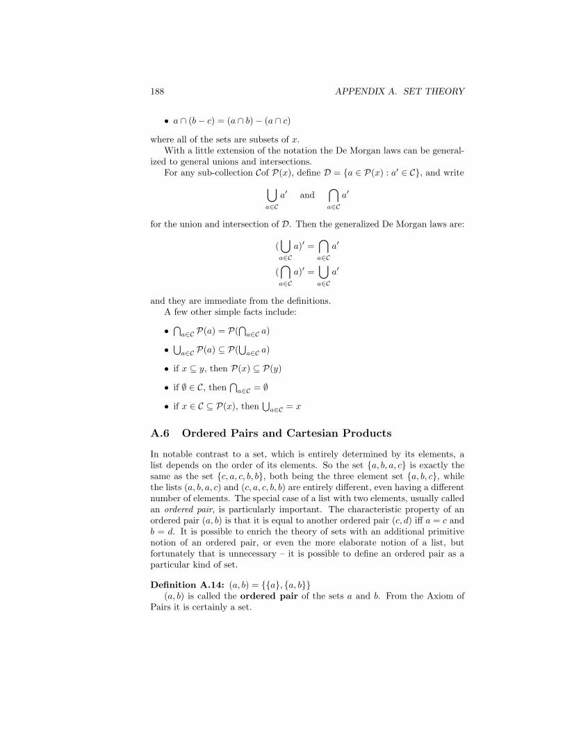
188 APPENDIX A. SET THEORY
• a ∩ (b− c) = (a ∩ b)− (a ∩ c)
where all of the sets are subsets of x.With a little extension of the notation the De Morgan laws can be general-
ized to general unions and intersections.For any sub-collection Cof P(x), define D = a ∈ P(x) : a′ ∈ C, and write⋃
a∈Ca′ and
⋂a∈C
a′
for the union and intersection of D. Then the generalized De Morgan laws are:
(⋃a∈C
a)′ =⋂a∈C
a′
(⋂a∈C
a)′ =⋃a∈C
a′
and they are immediate from the definitions.A few other simple facts include:
•⋂a∈C P(a) = P(
⋂a∈C a)
•⋃a∈C P(a) ⊆ P(
⋃a∈C a)
• if x ⊆ y, then P(x) ⊆ P(y)
• if ∅ ∈ C, then⋂a∈C = ∅
• if x ∈ C ⊆ P(x), then⋃a∈C = x
A.6 Ordered Pairs and Cartesian Products
In notable contrast to a set, which is entirely determined by its elements, alist depends on the order of its elements. So the set a, b, a, c is exactly thesame as the set c, a, c, b, b, both being the three element set a, b, c, whilethe lists (a, b, a, c) and (c, a, c, b, b) are entirely different, even having a differentnumber of elements. The special case of a list with two elements, usually calledan ordered pair, is particularly important. The characteristic property of anordered pair (a, b) is that it is equal to another ordered pair (c, d) iff a = c andb = d. It is possible to enrich the theory of sets with an additional primitivenotion of an ordered pair, or even the more elaborate notion of a list, butfortunately that is unnecessary – it is possible to define an ordered pair as aparticular kind of set.
Definition A.14: (a, b) = a, a, b(a, b) is called the ordered pair of the sets a and b. From the Axiom of
Pairs it is certainly a set.

A.6. ORDERED PAIRS AND CARTESIAN PRODUCTS 189
Proposition A.25 (a, b) = (c, d) iff a = c and b = d
Halmos [29, Section 6] has a nice explanation as to how this definition arises,and also proves the proposition. This proposition is also proved as Theorem1.33 in Monk [58] and on page 259 of Kelley [36]. The proofs are all somewhatdifferent in interesting ways.
The primary reason for introducing ordered pairs is to allow the followingdefinition.
Definition A.15: A×B = (a, b) : a ∈ A, b ∈ BA×B is called the Cartesian product of the classes A and B.
For any sets A and B, if a ∈ A and b ∈ B, then both a and a, b aresubsets of A ∪ B and so elements of P(A ∪ B). Thus (a, b) = a, a, b isa subset of P(A ∪ B) and so an element of P(P(A ∪ B)). This makes it clearthat A× B = (a, b) : a ∈ A, b ∈ B is a subset of P(P(A ∪ B)).
The sole purpose of introducing the rather odd definition of an orderedpair was to allow the construction of Cartesian products without introducingan independent concept and additional axioms. The definition itself will notbe used going forward, but only the basic property that (a, b) = (c, d) iff a = cand b = d. Thus, for example, the strange fact that a, b is an element of(a, b) will not be used, and is a somewhat embarrassing artifact. It is one ofthe reasons that fans of category theory are often annoyed by axiomatic settheory as the modern foundation for mathematics. A good explanation of thisperspective is given in Barr [2].
As you should suspect this is not the only possible construction that willserve as an ordered pair. For example defining [a, b] = ∅, a, ∅, b youcan readily prove that [a, b] is a set and that [a, b] = [c, d] iff a = c and b = d.The choice of what to use as the actual definition of an ordered pair is largelyarbitrary.
As with previous constructions, we record some basic facts about Cartesianproducts which will be used freely when needed: For A, B, X and Y any setswe have
• A × B 6= ∅ iff A 6= ∅ and B 6= ∅.
• If A ⊆ X and B ⊆ Y, then A× B ⊆ X × Y.
• If A× B 6= ∅ and A× B ⊆ X × Y, then A ⊆ X and B ⊆ Y.
• (A ∪ B)×X = (A×X ) ∪ (B × X ).
• (A ∩ B)×X = (A×X ) ∩ (B × X ).
• (A− B)×X = (A×X )− (B × X ).
Products are a fundamental notion in category theory with the Cartesianproduct of sets as the basic example, but we can not yet discuss the category

190 APPENDIX A. SET THEORY
of sets using axiomatic set theory as we do not yet have functions! Functionswill actually be defined via Cartesian products, and first we discuss the moregeneral notion of relations.
Even more, here in set theory the fundamental notion is really the orderedpair and Cartesian products ARE particular sets of ordered pairs, while inthe category Set the particular object is not important, only the UniversalMapping Property of the object together with its projection morphisms (whichwe have not yet even defined!)
A.7 Relations
Throughout this section script letters such as A, B, X , Y and R, as well assmall letters, will denote sets so that we can conveniently write a ∈ A, etc.with the implication that A is a set of sets.
Definition A.16: A relation from X to Y is a subclass of X × Y .
This is often called a binary relation, and ternary and even general n-aryrelations are defined as subsets of X×Y ×Z and of X1×· · ·×Xn respectively.In this appendix we will restrict attention to binary relation and just refer tothem as relations.
There are other closely related definitions as well.
Definition A.17: If R is a relation from X to Y , the domain of definitionof R is the class
domain(R) = x ∈ X : ∃y ∈ Y [(x, y) ∈ R]
Definition A.18: The range of R is the class
range(R) = y ∈ Y : ∃x ∈ X [(x, y) ∈ R]
For every relation R from X to Y we have domain(R) ⊆ X and range(R) ⊆Y , and both of these inclusions may be strict.
When X and Y are sets, any relation from X to Y is a set, as are thedomain of definition and range of the relation.
By contrast to the definition here it is usual to define a relation to beany class of ordered pairs. It is then easy to see that a relation R will be asubclass of domain(R)× range(R). The reason for the different definition hereis for convenience in discussing the category of relations (see Section B.1.3.)A notational confusion arises as a result – usually the domain of definition ofa relation is simply called the domain, but in the category Rel a morphism

A.7. RELATIONS 191
from the set X to the set Y is a relation from X to Y so X is the domain(and Y is the codomain of the relation.) Hence our use of the term domain ofdefinition even though we still write domain(R). In practice this seldom causesconfusion.
Examples of relations include:
• The empty set is a relation from any class to any other class.
• X × Y is a relation from X to Y .
• The equality relation or diagonal on any class X is the class (x, x) :x ∈ X. We usually denote this by EX or ∆X . The subscript X willbe omitted if it is clear. In particular there is EV with V the universalclass. This is usually denoted by just E or ∆. Observe that for any classX we have ∆X = ∆ ∩X.
• For any set X there is the relation E from X to P(X ) with E = (x,A) :x ∈ A.
There is a variety of notation, terminology and definitions that we need torecord. If R is a relation, we usually write xRy instead of (x, y) ∈ R. If R is arelation from X to itself we say that R is a relation on X.
In all of the following definitions, R is a relation on X.
Definition A.19: R is reflexive iff xRx for every x ∈ X.
Definition A.20: R symmetric iff xRy implies yRx.
Definition A.21: R is antisymmetric iff xRy and yRx implies x = y.
Definition A.22: R is connected iff always xRy or yRx.
Definition A.23: R is transitive iff xRy and yRz implies xRz.
Definition A.24: R is an equivalence relation iff it is reflexive, symmetricand transitive.
The fundamental equivalence relation on any class is the equality relation.As classes, relations from X to Y can be compared to see if they are sub-
classes of one another. A relation R is smaller or finer than a relation S whenR ⊆ S. Equally well we say that S is larger or coarser than R. With thisterminology, a relation R on X is reflexive iff it is coarser than the equalityrelation.
Other important special types of relations, partial orders, are discussed atlength in Section A.12.

192 APPENDIX A. SET THEORY
Associated to each relation from X to Y is the opposite or inverse rela-tion gotten by reversing the coordinates in each ordered pair in the relation.Symbolically
Rop = R−1 = (y, x) ∈ Y × X : (x, y) ∈ RObserve that a relation R on X is symmetric iff R = R−1.
Relations can also be composed as in the next definition.
Definition A.25: If R is a relation from X to Y and Sis a relation from Yto Z then the composition of R followed by S is
S R = (x, z) ∈ X × Z : ∃y ∈ Y with (x, y) ∈ R ∧ (y, z) ∈ S
As a trivial example, if R is any relation from X to Y and EX is the equalityrelation on X, then R EX = R. Of course if EY is the equality relation on Y,then equally well EY R = R.
A relation R on X is transitive iff R R = R.The intersection of any family of transitive relations on a set X is again
a transitive relation on X . For a particular relation R on X , the intersectionof the family of all transitive relations on X that include Rgives a smallesttransitive relation that is coarser thanR. This is called the transitive closureof R. The same thing is true about reflexive relations and symmetric relations,so we also have the reflexive closure and symmetric closure of any relationR on X .
These closures can be described in other ways as well. The reflexive closureof a relation R is E ∪ R, with E the identity relation, while the symmetricclosure of R is R ∪ R−1. The transitive closure of R can be described interms of R R, R (R R) and so on, but the details will have to wait untilSection A.10. This alternative description actually allows us to define thetransitive closure on an arbitrary relation, not just a relation on a set.
In the same vein, the intersection of any family of equivalence relationson X is an equivalence relation on X , so the intersection of the family of allequivalence relations on X that are larger than R is the smallest equivalencerelation on X includingR. This is called the equivalence relation generatedby R. The alternative description of the transitive closure also allows us todefine the equivalence relation generated by an arbitrary relation, not just arelation on a set.
Equivalence relations are tightly intertwined with two other basic notions– partitions and quotient sets.
Definition A.26: When R is an equivalence relation on X and x ∈ X, theequivalence class of x with respect to R is the class y ∈ X : xRy.
The basic property of equivalence classes is the following proposition.
Proposition A.26 With R an equivalence relation on X, x/R = y/R ⇐⇒xRy.

A.7. RELATIONS 193
There is no really common notation for equivalence classes, but we willusually write x/R. When X is a set the equivalence classes for any relation onX are subsets of X. When X is a proper class, the status of the equivalenceclasses is varied. For example on any classX and any element x, the equivalenceclass for the equality relation is the set x/E = x. At the other extreme takingR to be the equivalence relation X ×X on X, all elements are equivalent andso the one equivalence class is X itself. So if X is a proper class, then so is thisequivalence class. All kinds of mixtures of sets and proper classes are possible.
Our primary interest in equivalence relations is because of their connectionwith quotient sets (see I.26.)
Definition A.27: X/R = y ∈ P(X ) : ∃x ∈ X (y = x/R)With R an equivalence relation on the set X , the set X/R is called the
“quotient of X by R.” It is also called “X modulo R” or “X mod R”. Suchsets in general are called quotient sets.
As a collection of sets X/R has three characteristic properties. First it isdisjoint.
Definition A.28: Two classes A and B are disjoint when A∩B = ∅. A classX is disjoint provided any two distinct members of X are disjoint.
X/R is disjoint, for if y ∈ x/R∩ z/R, then xRy and zRy so also yRz andthen xRy. Whereupon x/R = y/R.
Second every element of X/R is non-empty for (x, x) is always in x/R.Third the union of X/R is X for every x ∈ X belongs to exactly one
equivalence class, namely x/R.The process can be reversed, and for that we start with the relevant defini-
tion.
Definition A.29: A partition of a set X is disjoint collection of non-emptysubsets of X whose union is X .
Given a partition P of X , define a relation R by saying
xRy iff ∃s ∈ R such that x ∈ s ∧ y ∈ s
Then R is an equivalence relation: X is the union of P, so each x ∈ X belongsto some set in P. As x is certainly in the same set as itself, this says that R isreflexive. R is symmetric for if x and y are in the same s ∈ P, then certainlyy and x are both in s. And finally R is transitive because this is just sayingthat if x and y are in the same set and y and z are in the same set, then x andz are in the same set.
So an equivalence relation R gives a partition P, while P in turn gives anequivalence relation which is clearly seen to be R. In the other direction, anypartition P gives rise to an equivalence relation where the set of equivalenceclasses is P.

194 APPENDIX A. SET THEORY
Just as with products, the quotient of a set X by an equivalence relationRreally IS a specific subset of P(X ), while in the category Set the particularobject is not important, only the universal mapping property of the quotientfunction (which we’ll finally define in the next section!)
A.8 Functions
The mathematical term “function”, as a magnitude associated to a curve, wasintroduced by Leibniz late in the 17th century. By the mid 18th century Eulerwas using function to describe an analytic expression, e.g. sin(x3). During the19th century many and varied “monster” functions were discovered: Dirichlet’sexample of a function that is continuous nowhere, or worse a function that iscontinuous at the irrational numbers and discontinuous at the rational numbers;Weierstrass’ function that is continuous everywhere but nowhere differentiable;and various examples of space-filling curves. Cantor’s introduction of set theorywas motivated by his efforts to understand the variety of functions, particularlythose represented by Fourier series. His own first shocking result was in showingthat the unit interval was in one-to-one correspondence with the unit square.Throughout this period the concept of function was gradually being clarifiedand finally reached is current form in the early 20th century.
Because of this long history there are many other words such as map, map-ping, transformation, correspondence, and operator that have been used assynonyms for function. And even today we frequently find such definitions as“A variable so related to another that for each value assumed by one there is avalue determined for the other”, “A correspondence in which values of one vari-able determine the values of another”, or “A rule for associating a member ofone set with a member of another set.” Although the spirit of these definitionsis different, the actually utility is well captured by the following definition.
Definition A.30: A function from the class X to the class Y is a relationF from X to Y with the property that for every x ∈ X there is a uniquey ∈ Y with (x, y) ∈ F . That unique y with (x, y) ∈ F is denoted by F (x). Forfunctions the notation y = F (x) is universally used in place of (x, y) ∈ F andxFy
The notation F : X // Y means “F is a function from X to Y ”. Aswith any relation, a function F : X // Y has a domain of definition and arange. The domain of definition of F is X which is also the domain of F as amorphism in the category of sets. The range may be a proper subclass of Y .More, a function from X to Y does not determine Y . In the category of sets,Y is the codomain of F . The fact that a function does not specify its codomainis the reason that the morphisms in the category of sets are not just functions.
At times many of the words mentioned above will be used as synonyms forfunction. In particular we will freely use the phrase binary operation on X fora function from X ×X to X.

A.8. FUNCTIONS 195
Just as with relations in general, if X and Y are sets then every functionfrom X to Y is a set, being a subset of X × Y .
When the range of F is equal to Y , we say that F maps X onto Y or,more commonly today, that F is surjective or is a surjection. We may also saythat F is an epimorphism though this is usually reserved for those cases wherethe functions of interest are called homomorphisms.
When we write y = F (x) we will speak of the argument x and of y as thevalue of F at x.
What we here define to be a function is what is often called the graph of thefunction. For example in elementary mathematics it is common to distinguishbetween the function sin(x) and it’s graph (x, sin(x)) ∈ R2 : x ∈ R. Buthere no distinction is made between the two, as all the relevant properties ofthe function are captured by its graph.
The range of F is also commonly called the image of F . When A is anysubset of X, the subset
F (A) = y ∈ Y : ∃x ∈ A [y = F (x)]
of Y is called the image of A under F . Of course F (X) is the image of F .If Y is not empty, the simplest examples of functions are the constant
functions: if y ∈ Y , then X × y ⊆ X × Y is a constant function which hasthe value y at every argument x.
For X a subset of Y , the set X × X is a function i :X // Y called theinclusion or injection of X into Y . A far more common way of describing i isto say it is the function defined by i(x) = x for all x ∈ X. The phrase “thefunction F defined by . . . ” is the most common way of defining functions, andis intended to imply there is a unique function defined by specifying the valuey of the function at each argument x. For example, we usually use y to namea constant function what has always the value y.
In the special case ofX considered as a subset of itself, the inclusion functionis called the identity function: 1X : X // X is defined by 1X(x) = x. Ofcourse this is just another name for the equality relation on X.
If F : X // Y and G : Y // Z, then we have the composition G F as arelation from X to Z. This is again a function and is just called the compositionof the functions. It is often written as just GF . As noted earlier with regardto relations F1X = F and 1Y F = F . Also if z is a constant function from Y
// Z, then zF = z, the second z being the constant function from X to Z.And if y is a constant function from X to Y , then Gy = G(y), where G(y) isthe constant function from X to Z with value G(y).
When X is a subset of Y and F : Y // Z, we have the inclusion i : X// Y and the composition Fi. This composition is called the restriction of
F to X and is written F |X . If G : X // Z and F |X = G, then F is calledan extension of G to Y .
For any two classes X and Y we have the Cartesian product X × Y . Twovery important functions in this situation are the coordinate projectionsπ1 : X × Y // X and π2 : X × Y // Y defined by π1(x, y) = x andπ2(x, y) = y.

196 APPENDIX A. SET THEORY
Here we are deliberately violating our notational convention and using thelower case letter π for a function that may be a proper class. As in the notesproper the capital letter Π will be reserved for products.
Looking at the actual definition of π1 as a subset of (X×Y )×X, especiallytaking it all the way back to the definition of ordered pairs, illustrates theimportance of abstracting away the crucial properties. Getting away fromany such definitional complexity to the critical universal mapping property ofproducts in the category Set is another such step.
Another general example of a function comes from an equivalence relation.For any equivalence relation R on the set X , define the quotient map q : X
// X/R by q(x) = x/R. Clearly q is surjective. [For the significance of thisin the categorical context, see 22.]
As shown in exercise I.31 every function f : X // Y defines an equivalencerelation on X via x ≡F x′ iff F (x) = F (x′). Now the projection map q : X
// X/ ≡f is always surjective, and as shown in exercise I.32 there is a uniquefunction f : X/ ≡f // Y with f = fq.
The function f has the important property that if f(x/ ≡f ) = f(x′/ ≡f ),then x/ ≡f= x′/ ≡f .
A function F : X // Y is called one-to-one or, more commonly today,injective or an injection when F (x) = F (x′) ⇒ x = x′. We may also say thefunction is a monomorphism though this is usually reserved for those caseswhere the functions of interest are called homomorphisms.
A function that is both an injection and a surjection (i.e., is one-to-one andonto) is called a bijection.
Every function F : X // Y , considered as a relation, has an inverserelation F−1. If the inverse relation is also a function, then F is a bijection.Conversely if F is a bijection, then F−1 is a function. When F is a bijection,then F−1 F = 1X and F F−1 = 1Y . If X and Y are two sets where thereexists a bijection between them, then we will write X ∼ Y and say the two setsare bijective, equivalent, equinumerous, equipotent or have the same number ofelements. Of course we haven’t yet defined “number of elements”, so the lastphrase is a bit premature, but we will rectify that in Section A.9.
For sets X and Y, the class of all functions from X to Y is a subset ofP(X ×Y) and is denoted by YX . The reason this is written as an exponentialshould become clear in Section A.11 when we actually define an exponentialfunction.
Some basic properties of YX include the following:
• For every set Y, including the empty set, Y∅ = ∅.
• If X is not the empty set, then ∅X = ∅.
• P(X ) ∼ 2X : Let 2 denote a set with exactly two distinct elements (whichwe will call 0 and 1). For any set X consider the set 2X . Whenever A isa subset of X , define the characteristic function of A to be
χA : X // 2 with χA(x) = 1 if x ∈ A, χA = 0 otherwise

A.8. FUNCTIONS 197
From this we get the function from P(X ) to 2X defined by A 7→ χA, andthis function is a bijection. The inverse function is given by associatingto any map χ : X // 2 the subset x ∈ X : χ(x) = 1.
• (ZY)X ∼ Z(X×Y): The bijection from (ZY)X to Z(X×Y) is given byφ 7→ Φ where Φ(x, y) = φ(x)(y). The inverse is just gotten by readingthis formula the other way – a function Φ of two variables defines afunction of the first variable (x) whose value is a function of the secondvariable (y). In theoretical computer science this process of going from afunction of two variables to a function of one variable with values beingother functions is called currying in honor of the logician Haskell Curry,though this observation long predates Curry.
• There are other variations on the idea that sending a function to itsvalue at a particular argument defines a function whose arguments arefunctions. The simplest version of this is the function
eval : X // Y(YX )
defined by eval(x)(f) = f(x).
A.8.1 Families and Cartesian Products
There are many situations where functions are used in a fashion that leadsto very different notation and terminology. The most familiar examples aresequences such as 1, 1/2, 1/3, 1/4, . . . where nearly all the details of thefunction are at best implicit. (Sequences will be explicitly defined in the nextsection.)
The functions of interest here are called indexed families or just families.A family is a function x from an index set I to the indexed setX. An elementi of I is called an index, while the value of x at i is called the i − th termand is denoted by xi. In this section we will be discussing families of sets, andthe common terminology is something like “a family Ai of subsets of X” bywhich we understand a function from some index set I to P(X). It is evenmore common to use just “a family Ai of sets” leaving both the index setand the indexed set unspecified!
If Ai is a family of sets of X, then the union of the family, written⋃i∈I
Ai or even⋃i
Ai,
is the union of the range of the family. From the definition of union we seethat x ∈
⋃iAi iff x belongs to Ai for at least one i in I.
Similarly the intersection of a family Ai of sets, written⋂i∈I
Ai or even⋂i
Ai,

198 APPENDIX A. SET THEORY
is the intersect of the range of the family. Unlike unions this only makes sense ifthis is a non-empty family, i.e., the index set is non-empty. From the definitionof intersection we see that x ∈
⋂iAi iff x belongs to Ai for every index i.
The basic identities about unions and intersections that were listed for threesets in Section A.5 generalize immediately to families:
• B ∩⋃iAi =
⋃i(B ∩Ai)
• B ∪⋂iAi =
⋂i(B ∪Ai)
• (⋃iAi) ∩ (
⋃j Bj) =
⋃i,j(Ai ∩Bj)
• (⋂iAi) ∪ (
⋂j Bj) =
⋂i,j(Ai ∪Bj)
where Ai and Bj are families of sets and B is a set, and the notation⋃i,j
is shorthand for⋃
(i,j)∈I×J .In discussing unions and intersections of families, this is nothing but a
convenient if sloppy notation as the collections could be used equally well.And the reverse is true as well as any collection can be considered as a familyindexed by itself. But when generalizing Cartesian products families, in oneguise or another, are essential.
Definition A.31: If Xi is a family of sets with index set I, the Cartesianproduct is the set of all families xi with xi ∈ Xi for every i in I. It isdenoted by
Πi∈IXi or ΠiXi
As ΠiXi ⊆ (⋃iXi)I , so it is a set.
For each j ∈ I, the projection on the j-th coordinate is the functionπj : Πi∈IXi
// Xj defined by πj(xi) = xj
If Xi is a family of sets with index set 1, 2 with 1 and 2 being twounspecified but unequal elements, then we have both
X1 ×X2 and Πi∈1,2Xi
As these have been defined, they are very different sets, nonetheless itis customary to identify the set Πi∈1,2Xi of functions with the Cartesianproduct X1 ×X2 a set of ordered pairs as defined earlier. The justification isa “natural” bijection between the two sets. In the category Set, both of thesesets together with their projections are products of X1 and X2, and the naturalbijection is just the unique function between the two that commutes with theprojections.
There are a pair of equations that relate unions, intersections and Cartesianproducts:
• (⋃iAi)× (
⋃j Bj) =
⋃i,j(Ai ×Bj)
• (⋂iAi)× (
⋂j Bj) =
⋂i,j(Ai ×Bj)

A.9. NATURAL NUMBERS 199
where, of course, the intersections must be of non-empty families.All of the classes in this section were assumed to be sets, but much of
the discussion can be carried through for classes more generally. It is a goodexercise to verify just how much can be done.
A.8.2 Images
Every relation R from X to Y defines two functions between the power sets ofX and Y. The first is R : P(X ) // P(Y) defined by
R(A) = y ∈ Y : ∃a ∈ A (aRy)
for every subset A of X , while the second is R−1 : P(Y) // P(X ) defined by
R−1(B) = x ∈ X : ∃b ∈ B (xRb)
for B any subset of Y.
Definition A.32: R(A) is the image or direct image of A under R.
In Bourbaki’s useful phrase [9, p. VI] the use of R as the name of thefunction as well as the relation which produces it is an abuse of notation, butit improves readability while seldom creating confusion.
Definition A.33: R−1(B) is the inverse image of B under R.
R−1(B) has another possible meaning, the image of B under the relationR−1. Happily the two meanings are the same.
A.9 Natural Numbers
In Section A.8 we said that two sets have the same number of elements whenthey are bijective, i.e., there is a bijection between them. This equinumerousrelation between sets is an equivalence relation on the universe V :
1. Every set is equinumerous with itself – the identity function is a bijectionfrom the set to itself.
2. If X is equinumerous with Y , then Y is equinumerous with X – for ifthere is a bijection from X to Y , then its inverse is a bijection from Y toX.
3. If X is equinumerous with Y and Y is equinumerous with Z, then X isequinumerous with Z – for if f is a bijection from X to Y and g is abijection from Y to Z, then gf is a bijection from X to Z with inversef−1g−1.

200 APPENDIX A. SET THEORY
This suggests defining the “number of elements” in a set to be the equinu-merous equivalence class of that set. But with the exception of the equiva-lence class of ∅ (which is ∅) all of the equivalence classes are proper classes,i.e., there is not even a class of “numbers”. An alternative approach is to definenumbers to be certain canonical sets, one from each such “equivalence class”and that is what will be done here. Eventually we will associate to every set a“cardinal number” as the number of elements in the set. But the first step isto define the natural numbers 0, 1, 2, . . . within set theory.
The starting point is the number zero, and for that there is only one pos-sibility.
Definition A.34: The number zero is the empty set. When we are speakingof it as a number it will, of course, be written as 0.
The next step is to introduce a standard method for getting the next largernumber. The very natural idea is to define n + 1 = 0, 1, · · · , n. Notice thatas n should be 0, 1, · · · , n − 1 we can equally write this as n + 1 = n ∪ nwhich is very fortunate as we can make that a quite general definition.
Definition A.35: For any set x, the successor of x, written x+, is x ∪ x.
So 0+ = 0 and has a single element. Of course we are going to name it1. Similarly 1+ = 0, 1 is a set with two elements, and it will be called 2.We can keep going in this fashion as long as we want, but nothing we have yetguarantees the existence of a set of all the successors of 0. For that we needanother axiom.
Axiom of Infinity: There exists a set containing 0 and containing thesuccessor of each of its elements.
Solely for the purposes of the following discussion, we say that a set Ω isa successor set provided 0 ∈ Ω and x ∈ Ω ⇒ x+ ∈ Ω. The Axiom of Infinityguarantees that at least one such set exists, and because Ω+ is also a successorset there are many others. More importantly there is a smallest successorset. The intersection of any family of successor sets is a successor set, so theintersection of all successor sets in Ω is itself a successor set which is denoted byω. The set ω is actually a subset of every successor set (for if S is an successorset, then S ∩ω is a both a subset and a superset of ω and so must be ω.) Withthese preliminaries we make the following definition.
Definition A.36: The minimal successor set ω which is a subset of everysuccessor set is the set of natural numbers, and the elements of ω are callednatural numbers.
The justification for calling ω the set of natural numbers is in the nexttwo sections where the connection with the Peano Axioms and arithmetic areexplored.

A.9. NATURAL NUMBERS 201
The use of ω to denote the set of natural numbers is common, but notuniversal, in the literature of set theory, so it will be used throughout thisappendix. Elsewhere in these notes the notation N is used consistently for theset of natural numbers.
Definition A.37: A family with index set ω is called an infinite sequence,while a family with index set a natural number is called a finite sequence.
If ai is a finite sequence of sets indexed by the natural number n+, thenthe union of the sequence is denoted by
n⋃i=0
ai or a0 ∪ · · · ∪ an.
Similarly if ai is an infinite sequence of sets, then the union of the sequenceis denoted by
∞⋃i=0
ai or a0 ∪ a1 ∪ · · · .
Similar notation is used for intersections and Cartesian products of se-quences:
n⋂i=0
ai or a0 ∩ · · · ∩ an.
Πni=0ai or a0 × · · · × an.
∞⋂i=0
ai or a0 ∩ a1 ∩ · · · .
Π∞i=0ai or a0 × a1 × · · · .
There are a number of other uses of the word “sequence” which are allvariations on this. We will freely use such notation as
∞⋃i=3
ai
with the expectation that the meaning is clear.

202 APPENDIX A. SET THEORY
A.10 Peano Axioms
This section is a digression from the development of axiomatic set theory tojustify calling ω the set of natural numbers, and also to indicate the initial partof the development of (nearly) all of mathematics from set theory.
The starting point are the axioms for the foundation of arithmetic whichwere introduced by Giuseppe Peano in his book Arithmetices principia, novamethodo exposita published in 1889.
Recast in more modern language Peano showed the set N of natural numberscould be specified by the following Peano axioms.
1. 0 ∈ N.
2. Every natural number n has a successor, denoted n′.
3. 0 is not the successor of any natural number.
4. If n′ = m′, then n = m.
5. (Induction Principle) If Q ⊆ N with
• 0 ∈ Q, and
• q ∈ Q⇒ q′ ∈ Q
then Q = N.
The successor on n is what we commonly call n+ 1 (but the Peano Axiomsallow us to define addition and prove that n′ = n+ 1.)
The Induction Principle captures what is often call the Principle of Math-ematical Induction and stated as:
Let p(n) be a proposition depending on integer variable n. If p(0) is trueand ∀k ≥ 0[p(k)⇒ p(k + 1)], then p(n) is true for all n ≥ 0.
The Principle of Mathematical Induction follows from Peano’s InductionPrinciple by taking Q = n ∈ N : p(n). Q contains 0 because p(0) is trueby assumption, and k ∈ Q ⇒ k′ ∈ Q exactly because p(k) ⇒ p(k + 1). Ofcourse we are cheating a bit because we have identified k′ with k + 1 and thejustification for that will actually happen in the next section.
Prior to showing that the Peano Axioms are, suitably construed, theoremsof set theory, we will explore some of the basic consequences of these axioms.To do that we first formalize the following variant concept.
Definition A.38: A Peano system consists of a set P together with adistinguished element p0 ∈ P and a function S : P // P satisfying:
1. ∀p ∈ P [p0 6= S(p)].
2. S is injective, i.e., S(p) = S(q)⇒ p = q.
3. (Induction Principle) If Q ⊆ P with

A.10. PEANO AXIOMS 203
• p0 ∈ Q, and
• p ∈ Q⇒ S(p) ∈ Q,
then Q = P .
As so often in mathematics, we will usually name a Peano system (P, p0, S)by just the set P . Of course this is an abuse of notation but is not likely tocause confusion.
The most basic property of Peano systems is the ability to give recursivedefinitions of functions as in the following theorem.
Theorem A.15 (Recursion Theorem) Let (P, p0, S) is any Peano system.If x0 is an element of a set X, and f is a function from X to X, then there is aunique function φ : P // X with φ(p0) = x0 and ∀p ∈ P [φ(S(p)) = f(φ(p))].
Proof: Uniqueness: Suppose we have φ : P // X with φ(p0) = x0 and∀p ∈ P [φ(S(p)) = f(φ(p))] and ψ : P // X with ψ(p0) = x0 and ∀p ∈P [ψ(S(p)) = f(ψ(p))] and consider the subset Q = p ∈ P : φ(p) = ψ(p).Certainly p0 ∈ Q as φ(p0) = x0 = ψ(p0). And if p ∈ Q, then φ(S(p)) =f(φ(p)) = f(ψ(p)) = ψ(S(p)), i.e., S(p) ∈ Q. So Q = P and φ = ψ.
This type of proof based on appeal to the Induction Principle is called proofby induction.
Existence: The proof of existence has two parts – construction φ as a rela-tion and then verifying that it is actually a function.
Consider relations F from P to X which have the two properties that(p0, x0) ∈ F and (p, x) ∈ F ⇒ (S(p), f(x)) ∈ F . The relation P × X is onesuch, so the set F of all such relations is non-empty. Define φ =
⋂F . Clearly
φ itself belongs to F , so if φ is a function the proof is complete.So it remains to verify that if both (p, x) ∈ φ and (p, y) ∈ φ, then x = y.
Define Q = p ∈ P : ∀x∀y[(p, x) ∈ φ ∧ (p, y) ∈ φ ⇒ x = y. A proofby induction will show that Q = P and complete the proof of the RecursionTheorem.
First note that p0 ∈ Q, for if not there is some y ∈ X different from x0 with(p0, y) ∈ φ. But then (p0, x0) is in the relation φ − (p0, y) because x0 6= y.Also if (p, x) is in φ − (p0, y), then so is (S(p), f(x)) for S(p) is guaranteednot to be p0 and so (S(p), f(x)) is certainly not the removed element (p0, y).This says that φ− (p0, y) is in F contradicting the definition of φ as
⋂F .
A very similar argument shows that p ∈ Q ⇒ S(p) ∈ Q. For suppose thatp ∈ Q, but S(p) /∈ Q. Then there is a unique element x with (p, x) ∈ φ, Thepair (S(p), f(x)) is in φ but assuming that S(p) is not in Q there must be anelement y, different from f(x), so that (S(p), y) ∈ φ as well. So consider therelation φ−(S(p), y). As above (p0, x0) ∈ φ−(S(p), y) because S(p) 6= p0.Similarly (q, z) ∈ φ − (S(p), y) ⇒ (S(q), f(z)) ∈ φ − (S(p), y). To seethis consider two possibilities – q = p and q 6= p. When q = p, it must bethat z = x and so f(z) = f(x) 6= y. But if q 6= p, then S(q) 6= S(p) and so

204 APPENDIX A. SET THEORY
(S(q), f(z)) 6= (S(p), y). Thus φ− (S(p), y) ∈ F contradicting the definitionof φ =
⋂F .
This completes the proof by induction that φ is a function, and so the proofof the Recursion Theorem.
It is worth noting that the proof of the recursion theorem uses all threeparts of the definition of a Peano system. Indeed the theorem would not betrue were any of the conditions removed from the definition.
A first consequence of the Recursion Theorem is that Peano Sets are essen-tial unique.
Theorem A.16 (Uniqueness of Peano Sets) If (P, p0, S) and (Q, q0, T ) aretwo Peano systems, then there is a unique bijection f : P // Q such thatf(p0) = q0 and ∀p ∈ P (f(S(p)) = T (f(p))).
Proof: (Uniqueness Theorem) When (P, p0, S) and (Q, q0, T ) are two Peanosets, the Recursion Theorem applies to guarantee there are functions f : P
// Q and g : Q // P satisfying f(p0) = q0, g(q0) = p0, f(S(p)) = T (f(p)),and g(T (q)) = S(g(q)). So then gf : P // P and fg : Q // Q have theproperties gf(p0) = p0, gf(S(p)) = S(gf(p)), fg(q0) = q0, and fg(T (q)) =T (fg(q)). But 1P satisfies same two properties as gf , while 1Q satisfies thesame two properties as fg. As the Recursion Theorem guarantees there is onlyone function function from P to P and one function from Q to Q having theseproperties we conclude that fg = 1P and gf = 1Q.
It is good to know that Peano systems are essentially unique, but this isnot very interesting unless at least one exists. That is the basic point of thedefinition of the set ω in the last section.
Theorem A.17 The set ω with 0 (i.e., the empty set) as distinguished elementand S(n) = n+, is a Peano system.
Proof: To show that (ω, 0, S) is a Peano system we need to verify:
1. ∀n ∈ ω, 0 6= n+.
2. ∀n,m ∈ ω, n+ = m+ ⇒ n = m.
3. (Induction Principle) If Q ⊆ ω with
• 0 ∈ Q, and
• n ∈ Q⇒ n+ ∈ Q,
then Q = ω.
The first condition is clearly true as n ∈ n+, and so n+ 6= ∅. The InductionPrinciple is essentially the definition of ω: Q ⊆ ω and Q is a successor set,while by definition ω is contained in every successor set. Ergo Q = ω.
Curiously only the second condition (n,m ∈ ω(n+ = m+ ⇒ n = m)requires significant work, and it requires a small detour into some of the arcane

A.10. PEANO AXIOMS 205
points of set theory. Most applications of set theory discuss only sets and theirelements. Occasionally discussion of families of sets is required, but discussioninvolving long ∈-chains, i.e., a ∈ b ∈ c ∈ · · · just do not arise. By contrast theydo occur in the internals of set theory and this is the first illustration. Thisdiscussion will recur in the discussion of well-ordering and ordinal numbers.Recall that 0 ∈ 1 ∈ 2 ∈ · · · . That relationship is captured in the next definition.
Definition A.39: A set n is transitive provided ∀a∀b(a ∈ b∧b ∈ n⇒ a ∈ n).Equivalently n is transitive when ∀b(b ∈ n⇒ b ⊆ n).
To prove the second condition we will use the following two technical lem-mas.
Lemma 1 Every member of ω is transitive.
Lemma 2 ∀n ∈ ω(m ⊆ n⇒ m /∈ n)
Assuming the lemmas, suppose that n and m are natural numbers withn+ = m+. As n ∈ n+ = m+, so n ∈ m+ and thus n ∈ m or n = m. Bysymmetry we also have m ∈ n or n = m. If n 6= m, then n ∈ m and m ∈ n.The first lemma tells us that n is transitive and so n ∈ n. But as n ⊆ n thesecond lemma guarantees that n /∈ n. So we must have n = m.
Proof of Lemma 1: The proof is by induction. Consider the set S of alltransitive elements of ω. Trivially 0 ∈ S. If n ∈ S and k ∈ n+, then eitherk ∈ n or k = n. By assumption n is transitive, so if k ∈ n, then k ⊆ n andso k ⊆ n+. And if k = n, then certainly k ⊆ n+. So n+ ∈ S. The InductionPrincipal now applies to say S = ω which is the lemma.
Proof of Lemma 2: Again the proof is by induction. Let S = n ∈ ω :n ⊆ m ⇒ m /∈ n. Certainly 0 ∈ S as ∀m(m /∈ 0). Next assume n ∈ S. Notefirst that n ⊆ n, so our assumption means n /∈ n. Now consider some set mcontaining n+. This means n ⊆ m and n ∈ m. But then m /∈ n as n is in S,and m 6= n because n /∈ n, so m /∈ n+. The Induction Principal now applies tosay S = ω thereby completing the proof.
The technicalities occurring in these two lemmas and their proofs have verylittle to do with applications of set theory in other parts of mathematics, butthey will recur and be expanded in the development of the theory of ordinaland cardinal numbers later in this appendix.
We now have both existence and uniqueness of a Peano system, but notethat even though ω provides a very elegant and natural example of a Peanosystem it is not the only one. Indeed if (P, p0, S) is a Peano system, then sotoo is (P − p0, S(p0), S|P−p0). This corresponds to the observation thatproof by induction can start with 1 (or any other integer) rather 0.
Here are some fundamental facts about natural numbers that are easilyestablished directly from the Peano axioms:
• If n is any natural number, then n 6= n+.
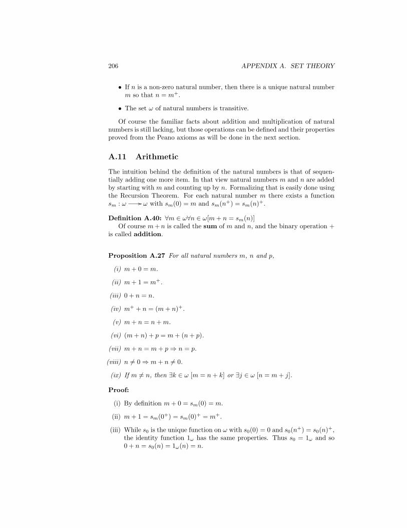
206 APPENDIX A. SET THEORY
• If n is a non-zero natural number, then there is a unique natural numberm so that n = m+.
• The set ω of natural numbers is transitive.
Of course the familiar facts about addition and multiplication of naturalnumbers is still lacking, but those operations can be defined and their propertiesproved from the Peano axioms as will be done in the next section.
A.11 Arithmetic
The intuition behind the definition of the natural numbers is that of sequen-tially adding one more item. In that view natural numbers m and n are addedby starting with m and counting up by n. Formalizing that is easily done usingthe Recursion Theorem. For each natural number m there exists a functionsm : ω // ω with sm(0) = m and sm(n+) = sm(n)+.
Definition A.40: ∀m ∈ ω∀n ∈ ω[m+ n = sm(n)]Of course m+n is called the sum of m and n, and the binary operation +
is called addition.
Proposition A.27 For all natural numbers m, n and p,
(i) m+ 0 = m.
(ii) m+ 1 = m+.
(iii) 0 + n = n.
(iv) m+ + n = (m+ n)+.
(v) m+ n = n+m.
(vi) (m+ n) + p = m+ (n+ p).
(vii) m+ n = m+ p⇒ n = p.
(viii) n 6= 0⇒ m+ n 6= 0.
(ix) If m 6= n, then ∃k ∈ ω [m = n+ k] or ∃j ∈ ω [n = m+ j].
Proof:
(i) By definition m+ 0 = sm(0) = m.
(ii) m+ 1 = sm(0+) = sm(0)+ = m+.
(iii) While s0 is the unique function on ω with s0(0) = 0 and s0(n+) = s0(n)+,the identity function 1ω has the same properties. Thus s0 = 1ω and so0 + n = s0(n) = 1ω(n) = n.

A.11. ARITHMETIC 207
(iv) The function sm+ is characterized by the two conditions: sm+(0) = m+
and sm+(n+) = sm+(n)+. But the function tm defined by tm(n) =sm(n+) satisfies those same two conditions. Therefore sm+ = tm and inparticular m+ + n = sm+(n) = tm(n) = sm(n+) = sm(n)+ = (m+ n)+.
(v) Consider S = m ∈ ω : ∀n ∈ ω[m + n = n + m]. Above saw that0 + n = n = n+ 0, so 0 is an element of S. And if m ∈ S, then
m+ + n = (m+ n)+ part 2 of this proposition= (n+m)+ because m in S= n+m+ by definition of addition
and so m+ ∈ S as well. The Induction Principal now applies to tell usthat S = ω and thereby completes the proof of this part.
(vi) The proof that (m+n) + p = m+ (n+ p) works by induction on p. Firstboth (m+ n) + 0 and m+ (n+ 0) are equal to m+ n by the definition ofaddition. For the induction step suppose that (m+ n) + p = m+ (n+ p)for all m and n. Then
(m+ n) + p+ = ((m+ n) + p)+ by definition of addition= (m+ (n+ p))+ by induction hypothesis= m+ (n+ p)+ by definition of addition= m+ (n+ p+) by definition of addition
and so the proof by induction is complete.
(vii) The proof thatm+n = m+p⇒ n = p is by induction onm. The assertionis certainly true for m = 0 as 0+n = n. So suppose that m++n = m++p.Then as m++n = m+n+, it follows that m+n+ = m+p+. The inductionhypothesis gives n+ = p+ and n = p follows from the fourth Peano Axiomand the proof by induction is complete.
(viii) This is also proved by induction on m. Certainly n 6= 0 ⇒ 0 + n 6= 0.Note that m+ +n = m+n+ and n+ is always non-zero, so the inductionhypothesis give m+ n+ 6= 0, so the proof by induction is complete.
(ix) Fix an arbitrary natural number n and consider the set
S = m ∈ ω : ∃k ∈ ω m = n+ k ∨ ∃j ∈ ω n = m+ j ∨
Certainly 0 ∈ S, so now for the induction step suppose that m ∈ S. Tosee that m+ is also in S the two cases:
(a) m = n + k – then m+ = n + k+. Note this includes the case thatk = 0 which is also the case n = m+ 0.
(b) n = m+ j with j 6= 0 – then there exists p ∈ ω with j = p+, and son = m+ j = m+ p+ = m+ + p.
So m+ ∈ S and so S = ω.

208 APPENDIX A. SET THEORY
At the same primitive level, multiplication of natural numbers can be con-sidered as repeated addition which can again be formalized using the RecursionTheorem: for each natural number there exists a m unique function pm : ω
// ω with pm(0) = 0 and pm(n+) = pm(n) +m.
Definition A.41: ∀m ∈ ω∀n ∈ ω[m · n = pm(n)]The natural number m ·n is called the product of m and n, and the binary
operation · is call multiplication.The · is often omitted with multiplication being indicated by juxtaposition
if no confusion will result. Other notation sometimes used in place of the · toindicate multiplication includes × and ∗.
Proposition A.28 For all natural numbers m, n and p,
(i) m · 0 = 0.
(ii) 0 · n = 0.
(iii) m · 1 = m.
(iv) (m · n) · p = m · (n · p).
(v) m · n = n ·m.
(vi) m · (n+ p) = (m · n) + (m · p).
(vii) if m 6= 1, then m · n = m · p⇒ n = p.
(viii) if n 6= 1, then m · n 6= 1.
The proof of this proposition is very similar to that of the preceding propo-sition and is omitted.
Finally the same process can be applied to exponents which arise from re-peated multiplication. Using the Recursion Theorem, for each natural numberm there exists a function em : ω // ω with em(0) = 1 and em(n+) = em(n)·m.
Definition A.42: ∀m ∈ ω∀n ∈ ω[mn = em(n)]The natural number mn is called the n-th power of m, and the operation
is called exponentiation.
Proposition A.29 For all natural numbers m, n and p,
(i) m0 = 1.
(ii) 0n = 0 except that 00 = 1.
(iii) m1 = m.

A.12. ORDER 209
(iv) (mn)p = m(np).
(v) m(n+p) = (mn) · (mp).
(vi) mn = mp ⇒ n = p except when mn is equal to 0 or 1.
(vii) mn = 1⇒ m = 1 ∨ n = 0.
The proof of this proposition is very similar to that of the preceding twopropositions and is omitted.
A.12 Order
The natural arithmetic operations (addition and multiplication) on the setω of natural numbers were developed in the previous section, but there isanother familiar and important aspect of the natural numbers that hasn’t yetbeen mentioned: order. The order relation in ω is the familiar succession0 < 1 < 2 < · · · . The first step is to make the order relation precise, andthat is based on the understanding that m is larger than n when m is gottenby from n by successive increments, which is the same as adding some naturalnumber to n.
Definition A.43: For all n,m ∈ ω, n ≤ m iff there is some natural number kso that m = n+ k.
In particular every natural number is equal to or greater than 0.
Proposition A.30 For all m, n and p in ω:
(i) (Reflexive) m ≤ m.
(ii) (Antisymmetric) m ≤ n ∧ n ≤ m⇒ m = n.
(iii) (Transitive) m ≤ n ∧ n ≤ p⇒ m ≤ p.
(iv) (Connected) Either m ≤ n or n ≤ m.
Proof: The proof is based on Proposition A.27. (i) is because m + 0 = m.For (ii) note that if m = n+ k and n = m+ l, then m+ 0 = m = (m+ l) + k =m + (l + k) and so l + k = 0 and so l = k = 0, i.e., m = n. (iii) comes fromnoting that if n = m + k and p = n + l, then p = (m + k) + l = m + (k + l).(iv) is just a restatement of the last part of Proposition A.27.
Order relations are both generally important and specifically important inthe study of infinite sets in set theory. The starting point here are some generaldefinitions and simple observations.
Definition A.44: A preorder on X is a relation R on X which is reflexive(∀x ∈ X, xRx), and transitive (∀x, y, z ∈ X, xRy ∧ yRz ⇒ xRz).

210 APPENDIX A. SET THEORY
Clearly the order relation on the natural numbers defined above is a pre-order.
Every preorder defines an equivalence relation: x ≡R y ⇐⇒ (xRy ∧ yRx).[Proof: x ≡R x because the preorder R is reflexive; x ≡R y ⇒ y ≡R x by thesymmetry in the definition of ≡R; and ≡R is transitive because R is transitive.]
The preorder also defines a preorder on the quotient set X/ ≡R in theexpected way: x/ ≡R Ry/ ≡R iff xRy. [Proof: If x ≡R x′ and y ≡R y′, andxRy, then xRy ∧ yRy′ ⇒ xRy′, while x′Rx ∧ xRy′ ⇒ x′Ry′. ]
This preorder on the quotient set now is antisymmetric, i.e., xRy and yRximplies x = y. An antisymmetric preorder is actually the usual basic object ofstudy in order theory and is formalized in the following definition.
Definition A.45: A partial order on X is a relation on X which is reflexive,transitive and antisymmetric.
Commonly a partial order is denoted by ≤ or something reminiscent suchas , ⊆, or v.
Proposition A.30 shows that the order relation on the natural numbers isnot just a pre-order, but a partial order.
Associated to a partial order ≤ on X are several other closely related rela-tions on X just as is familiar for order relation(s) on various types of numbers.For x and y in X, y ≥ x is the same as x ≤ y (i.e., ≥ is the inverse relation of≤,) The relation ≥ is also a (usually different) partial order on X.
For x and y in X, x < y means x ≤ y and x 6= y, and y > x is the sameas x < y. When x < y we say x is less than y, or smaller than y or precedesy. Similarly when y > x we say that y is greater than y, or larger than y orsucceeds or follows y.
The relation < is not a partial order, but gets its own definition.
Definition A.46: A strict order on X is a relation on X which is transitive,and anti-reflexive.
Commonly a strict order is denoted by < or something reminiscent such as≺, ⊂, or @.
Defining x < y to mean x ≤ y and x 6= y associates to a partial order ≤ astrict order <. Conversely starting with a strict order < and defining x ≤ y tomean x < y or x = y produces a partial order.
Definition A.47: A partially ordered set or, more commonly, a poset isa set together with a partial order on it.
Note that this is really just another name for a partial order (with domaina set) because a partial order determines the set on which it is a partial order!Despite this it is nearly universal to use the name of the domain of the partialorder to refer to the poset. The restriction to a partially ordered set rather than

A.12. ORDER 211
a partially ordered class is inessential but customary. The trivial extension ofwhat follows is left to the interested reader.
As discussed above, every poset has associated with it two partial ordersand two strict orders. This relationship is so intimate and so familiar that wewill freely move among the four relations with no comment at all.
The generic example of a partially ordered set is a power set P(x) with thesubset relation ⊆ as the partial ordering. Indeed any subset y of P(x) is aposet under the subset relation, and all posets are like that. Here is what thatmeans.
Definition A.48: If (a,≤) and (b,) are posets, then a monotone functionfrom a to b is a function f : a // b such that a1 ≤ a2 implies f(a1) f(a2).
Monotone functions are also called order preserving or isotone.
Definition A.49: An isomorphism between (a,≤) and (b,) is a monotonefunction from a to b with a monotone inverse f−1 : b // a.
Proposition A.31 If (a,≤) is a poset, then there is a subset b of P(a) with(a,≤) isomorphic to (b,⊆).
Proof: Associate to each element x of a the subset f(x) = y ∈ a : y ≤ xof a, and take b = f(x) : x ∈ a. This actually defines f as the desiredisomorphism. .
There are various special properties of partial orders that are of particularinterest.
Definition A.50: A connected partial order, i.e., for every x and y in X eitherx ≤ y or y ≤ x, is called a total order. (This is also called a linear order ora simple order.)
Definition A.51: A totally ordered set is a partially ordered set where thepartial order is a total order. A totally ordered set is often called a chain.
The full content of Proposition A.30 is that the order relation on the set ofnatural numbers is a total order.
Examples: Every equivalence relation is a partial order. Every pair of distinct ele-ments is incomparable. The only relation that is both a partial order andan equivalence relation is equality. The Hasse diagram of an equivalencerelation is a discrete graph, i.e., there are no edges.
Special Elements.
Definition A.52: A least element, minimum element, or first elementin a partially ordered set (X,≤) is an element x0 ∈ X such that ∀x ∈ X (x0 ≤x).

212 APPENDIX A. SET THEORY
Definition A.53: A greatest element, maximum element or last el-ement in a partially ordered set (X,≤) is an element x1 ∈ X such that∀x ∈ X (x ≤ x1).
A greatest element (X,≤) is a least element in (X,≥), and a least elementin (X,≤) is a greatest element in (X,≥). This is our first example of dualityfor order.
Least and greatest elements may fail to exist. For instance with our usualunderstanding of the ordering of the natural numbers, 0 is a least elementwhile there is no greatest element. But when they do exist least and greatestelements are clearly unique.
There are also the closely related but distinct notions of minimal and max-imal elements.
Definition A.54: A minimal element in a partially ordered set (X,≤) isan element x0 ∈ X such that x ≤ x0 ⇒ x = x0.
If x0 is a least element in X, then it is certainly a minimal element in X,but the converse is not true. Just as with least elements, minimal elements maynot exist in a particular poset. But, by contrast with least elements, minimalelements may not be unique even when they do exist.
The dual notion is that of maximal elements which are the minimal elementsfor the poset (X,≥). Here is the direct definition.
Definition A.55: A maximal element in a partially ordered set (X,≤) isan element x0 ∈ X such that x ≥ x0 ⇒ x = x0.
When (X,≤) is a poset and Y is a subset of X we define the relation ≤ |Yon Y to be ≤ ∩Y × Y . Usually we will just speak of the inherited order on Yand use the same symbol for the partial order on Y as for the partial order onX.
There are several special elements associated to subsets of a poset.
Definition A.56: An upper bound for a subset Y of a poset X is an elementx ∈ X with ∀y ∈ Y y ≤ x
Dually we have lower bounds.
Definition A.57: A lower bound for a subset Y of a poset X is an elementx ∈ X with ∀y ∈ Y y ≥ x
Of special interest are least elements among upper bounds and greatestelements among lower bounds, so we have the following definitions.
Definition A.58: Associated to each subset Y of the poset X we have thesubset U consisting of all upper bounds of Y . A least element of U is calleda least upper bound of Y . As with least elements in general, this may not

A.13. NUMBER SYSTEMS 213
exist, but is unique when it does exist. A least upper bound is also commonlycalled a supremum or a lub, and denoted lub(Y ) or
∨(Y ).
Definition A.59: Associated to each subset Y of the poset X we have thesubset L consisting of all lower bounds of Y . A greatest element of L is calleda greatest lower bound of Y . As with greatest elements in general, thismay not exist, but is unique when it does exist. A greatest lower bound is alsocommonly called an infimum or a glb, and denoted glb(Y ) or
∧(Y ).
The order relations defined on the natural numbers were all defined usingthe properties of the set of natural numbers as a Peano system. This processcan also be reversed and the Peano system structure defined in terms of theorder relation. The first part is simply that 0 is the least element of the orderedset ω. The harder part is the definition of the successor function and proof ofthe induction principal. That will be done in Section A.16. Beyond that thereis an alternative perspective on the order relation that is more directly tied tothe details on how ω and its elements are defined that will be considered thereas well.
Duality in OrderSeveral times above we have remarked on pairs of dual concepts in a posets.
Examples of dual pairs include “least” and “greatest”, “minimal” and “maxi-mal”, “lower bound” and “upper bound”, and “lub” and “glb”.
Every order theoretic definition has its dual, obtained by applying the givendefinition to the inverse relation. Equally every theorem in order theory alsohas a dual theorem which does not require a separate proof.
The connection between posets and categories (see Section B.19.4) exposesduality in order as yet another example of duality of categories.
A.13 Number Systems
There are several number systems besides the natural numbers that are com-monly considered: integers, rational numbers, real numbers and complex num-bers. All of these can be defined, there existence demonstrated and their prop-erties proved within axiomatic set theory. One valuable classic on the topic isLandau’s Foundations of analysis; the arithmetic of whole, rational, irrational,and complex numbers [39], while two more recent treatments are The Struc-ture of the Real Number System [12] by Cohen and Ehrlich and The NumberSystems: Foundations of Algebra and Analysis [23] by Feferman.
The discussion of number systems is not very close to the theory of sets,but this is a convenient point to provide a precis of the material for referencein the remainder of the notes.
From Section B.2.3 of the Catalog we recall that a monoid consists of aset M and an associative binary operation on M that has an identity. If thebinary operation is commutative, then M is a commutative monoid

214 APPENDIX A. SET THEORY
Proposition A.32 The set of natural numbers with the binary operation ofaddition is a commutative monoid with 0 as the identity.
This is just another way of stating parts of Proposition A.27.
Proposition A.33 The set of natural numbers with the binary operation ofmultiplication is a commutative monoid with 1 as the identity.
This is just another way of starting parts of Proposition A.28.As there are two natural and common ways in which the set of natural
numbers are a monoid it is sometimes necessary to distinguish them. The setof natural numbers together with the binary operation of addition is called theadditive monoid of natural numbers, while when considering multiplication we
speak of the multiplicative monoid of natural numbers.
Proposition A.34 The additive monoid of natural numbers is a free monoidgenerated by 1.
Proof: This means that if (M, ·, 1) is any monoid and m0 is an arbitraryelement of M , there there is a unique monoid homomorphism h : ω // Mwith h(1) = m0.
As preparation to using the Recursion Theorem, define a function f : M// M by f(m) = m0 ·m. Then there is a unique function h : ω // M so
that h(0) = 1 and h(S(n)) = m0 · h(n). Then h(1) = h(S(0)) = m0 · 1 = m0.Next we use induction to prove that h is a homomorphism. Consider the
set Q = n ∈ ω : ∀n′ ∈ ω [h(n + n′) = h(n) · h(n′)]. Certainly 0 ∈ Q ash(0+n′) = h(n′) = h(0) ·h(n′) for h(0) = 1. And if n ∈ Q, then h(S(n)+n′) =h(S(n+n′)) = m0 ·h(n+n′) = m0 ·h(n) ·h(n′) = h(S(n)) ·h(n′), so S(n) ∈ Q.By the Induction Principle Q = ω and so h is a homomorphism.
Proposition A.35 The multiplicative monoid of positive natural numbers isa free monoid generated by the prime numbers.
The Abelian group of integers is constructed from the monoid of naturalnumbers in a fashion that applies in the following generality.
Proposition A.36 For every commutative monoid N there is an Abelian groupZ and a monoid homomorphism i : N // Z so that for every monoid homo-morphism h : M // A of M to an Abelian group A there is a unique grouphomomorphism H : Z // M so that h = Hi.
N Zi //N
A
h
Z
A
H
The pair (Z, i) is called Abelian group completion of the commutative monoidN .

A.13. NUMBER SYSTEMS 215
For the proof see Proposition B.39.Of course this is an example of a universal mapping property and as in all
such cases the Abelian group is unique up to isomorphism.
Definition A.60: The Abelian group of integers, Z, is the Abelian groupcompletion of the commutative monoid of natural numbers.
This “definition” has a problem. What exactly is the set Z? In particularis the set ω of natural numbers a subset of Z? Common mathematical usagecertainly assumes that every natural number is an integer! But it is also com-mon in the development of number systems from the axioms of set theory oreven from the Peano axioms to identify the set Z as a set of equivalence classesof pair of natural numbers as in the proof of Proposition B.39 so that ω is nota subset of Z. This is a minor but niggling annoyance which can be addressedin several different ways.
One solution is to change the definition of the natural numbers or theintegers so that the set of natural numbers is a subset of the set of integers.Again there are several possible ways of doing that with perhaps the simplestbeing to define the integers by just adjoining suitable negative integers to ω asis the common notation. Verifying that this works is a bit of a nuisance, butit certainly works.
Another solution is to provide an axiomatic characterization of the integers(for example as a certain type of ordered integral domain,) and show thatthe system of integers must have a compatible Peano system as a subsystem(which is, of course, isomorphic to the Peano system of natural numbers.) Thenarbitrarily fix one such as “the” integers and “the” natural numbers.
Still another approach is to incorporate additional axioms that define all ofthe usual number systems (natural numbers, integers, and rational, real andcomplex numbers) and ensure the expected inclusion relations. This involveschanging the approach used here so that there are elements (commonly calledurelements) besides those that are sets. Then the constructions here and inSection A.11 serve to show that the more complex axiom systems that definethe number systems are equiconsistent with the limited set theory axioms inthis Appendix.
Introducing urelements seems to refute the remark that “for the purposesof mathematics it seems to be enough to have just sets that can be built fromthe empty set” (page 182) but the use or lack of other elements is entirely amatter of convenience. (It is left as an exercise for the reader to decide wherethe convenience lies!)
As remarked in Section A.6 the same thing is equally well true for or-dered pairs. Rather than using the abstruse definition given in these notesit is entirely feasible to introduce them as independent entities having theircharacteristic property, and then allow ordered pairs of element as elements aswell. In the same vein it is also possible to introduce functions as new objectssubject to suitable axioms and then allow them to be elements of sets as well.The reason this is seldom done is because of the complexity associated with

216 APPENDIX A. SET THEORY
having many different logical entities and the large complicated collection ofaxioms needed to specify this complexity.
In this Appendix we will follow the same general approach we have usedthroughout the notes of being somewhat cavalier in accepting these numbersystems without completely specifying exactly the set at issue.
At this stage the set of integers as a mathematical object is defined as beinga certain Abelian group, while the set of integers so familiar to us all also hasmultiplication and an order relation extending the same features of the naturalnumbers.
A.14 Axiom of Choice
Axiom of Choice: The Cartesian product of a non-empty family of non-empty sets is non-empty.
A.15 Zorn’s Lemma
A.16 Well Ordered Sets
Definition A.61: A well ordered set is a poset in which every non-emptysubset has a least element.
Definition A.62: For a well ordered set X and x an element of X, thesegment of X determined by x is the set y ∈ X : y < x
Theorem A.18 Let (X,≤) be a well ordered set. Suppose that S is a subsetof X such that:
1. the smallest element of X is an element of S, and
2. ∀x ∈ X [∀y ∈ X (y < x⇒ y ∈ S)⇒ x ∈ S]
Then S = X.
A.17 Transfinite Induction
A.18 Axiom of Substitution
Axiom of Substitution: If f is a function and the domain of f is a set,then the image of f is a set.

A.19. ORDINAL NUMBERS AND THEIR ARITHMETIC 217
A.19 Ordinal Numbers and Their Arithmetic
A.20 The Schroder-Bernstein Theorem
A.21 Cardinal Numbers and Their Arithmetic
A.22 Axiom of Regularity
Axiom of Regularity:


Appendix B
Catalog of Categories
The purpose of this appendix is to catalog a variety of categories, togetherwith interesting properties and interrelations. It comes here at the end exactlybecause we feel free to discuss all of the notions that occur earlier in these notes.But the intention is that each section can be read only part way for informationrelevant to early parts of the notes. So in particular the properties of thesecategories are discussed in approximately the same order as those propertiesare discussed in the notes.
There are a substantial variety of categories discussed here, and it is unlikelythat all of them will be familiar to any reader of these notes. For just thatreason each section is intended to be largely independent of the other sections.Moreover we provide references for readers who want more information aboutthe particular categories. The references are not usually about the categoriesper se, but usually to sources where the objects and morphisms that constitutethe category and discussed.
Each of the “big three” topics in Mathematics: Algebra, Topology andAnalysis contribute a large number of categories that are familiar, by which wemean widely and commonly studied. Adding to those the categories associatedto the foundational topics of set theory, order and logic provides the sourceof most of the categories listed in this chapter. That also is the organizingprinciple, at least up to section B.16.
While the study of categories is fundamentally about morphisms, the fa-miliar categories are named after their objects. This is a reflection that thefirst level of abstraction was such objects as groups, rings, topological spaces,etc. The study of the morphisms between suitable objects came later. Evenwhen morphisms began to be studied, the starting point was objects as “setswith structure” and morphisms were just certain functions that “respected”the structure.
In most of the categories described below the identity function on (the un-derlying set of) an object is a clearly a morphism, and the function compositionof two morphisms is again a morphism and with these observations it is a trivialformality to verify that the proposed category is indeed a category. So in most
219
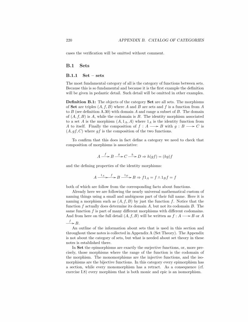
220 APPENDIX B. CATALOG OF CATEGORIES
cases the verification will be omitted without comment.
B.1 Sets
B.1.1 Set – sets
The most fundamental category of all is the category of functions between sets.Because this is so fundamental and because it is the first example the definitionwill be given in pedantic detail. Such detail will be omitted in other examples.
Definition B.1: The objects of the category Set are all sets. The morphismsof Set are triples (A, f,B) where A and B are sets and f is a function from Ato B (see definition A.30) with domain A and range a subset of B. The domainof (A, f,B) is A, while the codomain is B. The identity morphism associatedto a set A is the morphism (A, 1A, A) where 1A is the identity function fromA to itself. Finally the composition of f : A // B with g : B // C is(A, gf, C) where gf is the composition of the two functions.
To confirm that this does in fact define a category we need to check thatcomposition of morphisms is associative:
Af // B
g // Ch // D ⇒ h(gf) = (hg)f
and the defining properties of the identity morphisms:
A1A // f // B
1B // B ⇒ f1A = f ∧ 1Bf = f
both of which are follow from the corresponding facts about functions.Already here we are following the nearly universal mathematical custom of
naming things using a small and ambiguous part of their full name. Here it isnaming a morphism such as (A, f,B) by just the function f . Notice that thefunction f actually does determine its domain A, but not its codomain B. Thesame function f is part of many different morphisms with different codomains.And from here on the full detail (A, f,B) will be written as f : A // B or Af // B.
An outline of the information about sets that is used in this section andthroughout these notes is collected in Appendix A (Set Theory). The Appendixis not about the category of sets, but what is needed about set theory in thesenotes is established there.
In Set the epimorphisms are exactly the surjective functions, or, more pre-cisely, those morphisms where the range of the function is the codomain ofthe morphism. The monomorphisms are the injective functions, and the iso-morphisms are the bijective functions. In this category every epimorphism hasa section, while every monomorphism has a retract. As a consequence (cf.exercise I.8) every morphism that is both monic and epic is an isomorphism.

B.1. SETS 221
Set has an initial object, the empty set with the unique function ! fromthe initial object to any other object being the empty function. Set has manyfinal objects, namely all of the singleton sets with !, the unique function fromany object to the final object, being the function that sends every element tothe single element.
Set has products and sums. The product of two sets X and Y “is” theusual Cartesian product X×Y (see definition A.15) consisting of ordered pairsof elements from the two sets, with π1(x, y) = x and π2(x, y) = y. Of courseas is true is any category, if there is an isomorphism (i.e., a bijection in thiscontext) from Z to X × Y then composing the bijection with π1 and π2 givestwo projections morphisms from Z to X and Y which makes Z a product ofthe two sets as well.
The sum of sets is the less familiar disjoint union as discussed on page 35.By contrast, Lawvere and Rosebrugh (Sets for Mathematics) [46] give an
informal axiomatic treatment of the category of sets which does not depend onaxiomatic set theory as treated in the appendix.
Barr [2] provides a fine polemic explaining why categorical set theory ispreferable to traditional axiomatic set theory.
B.1.2 FiniteSet – finite sets
The category FiniteSet of finite sets is the full subcategory of Set whoseobjects are the finite sets.
Just as in Set the epimorphisms in FiniteSet are exactly the surjectivefunctions, or, more precisely, those morphisms where the range of the func-tion is the codomain of the morphism. The monomorphisms are the injectivefunctions, and the isomorphisms are the bijective functions. In this categoryevery epimorphism has a section, while every monomorphism has a retract. Asa consequence (cf. exercise I.8) every bimorphism, i.e., one that is both monicand epic, is an isomorphism.
The unique initial object in Set, namely the empty set, is also the uniqueinitial object in FiniteSet. And all of the many final objects in Set, namelyall of the singleton sets, are equally well the final objects in FiniteSet.
Also the products and sums in Set are equally well the products and sumsin FiniteSet, for the product and sum of two finite sets are also finite sets.
B.1.3 Rel – the category of sets and relations
The objects of Rel are sets, while the morphisms are relations between sets.(See Section A.7 for the relevant definitions.)
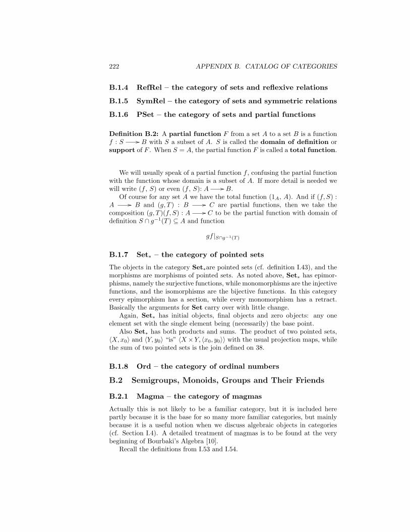
222 APPENDIX B. CATALOG OF CATEGORIES
B.1.4 RefRel – the category of sets and reflexive relations
B.1.5 SymRel – the category of sets and symmetric relations
B.1.6 PSet – the category of sets and partial functions
Definition B.2: A partial function F from a set A to a set B is a functionf : S // B with S a subset of A. S is called the domain of definition orsupport of F . When S = A, the partial function F is called a total function.
We will usually speak of a partial function f , confusing the partial functionwith the function whose domain is a subset of A. If more detail is needed wewill write (f , S) or even (f , S): A // B.
Of course for any set A we have the total function (1A, A). And if (f, S) :A // B and (g, T ) : B // C are partial functions, then we take thecomposition (g, T )(f, S) : A // C to be the partial function with domain ofdefinition S ∩ g−1(T ) ⊆ A and function
gf |S∩g−1(T )
B.1.7 Set∗ – the category of pointed sets
The objects in the category Set∗are pointed sets (cf. definition I.43), and themorphisms are morphisms of pointed sets. As noted above, Set∗ has epimor-phisms, namely the surjective functions, while monomorphisms are the injectivefunctions, and the isomorphisms are the bijective functions. In this categoryevery epimorphism has a section, while every monomorphism has a retract.Basically the arguments for Set carry over with little change.
Again, Set∗ has initial objects, final objects and zero objects: any oneelement set with the single element being (necessarily) the base point.
Also Set∗ has both products and sums. The product of two pointed sets,〈X,x0〉 and 〈Y, y0〉 “is” 〈X ×Y, 〈x0, y0〉〉 with the usual projection maps, whilethe sum of two pointed sets is the join defined on 38.
B.1.8 Ord – the category of ordinal numbers
B.2 Semigroups, Monoids, Groups and Their Friends
B.2.1 Magma – the category of magmas
Actually this is not likely to be a familiar category, but it is included herepartly because it is the base for so many more familiar categories, but mainlybecause it is a useful notion when we discuss algebraic objects in categories(cf. Section I.4). A detailed treatment of magmas is to be found at the verybeginning of Bourbaki’s Algebra [10].
Recall the definitions from I.53 and I.54.

B.2. SEMIGROUPS, MONOIDS, GROUPS AND THEIR FRIENDS 223
Definition: A magmais a set, M , together with a binary operation orlaw of composition, µ : M ×M // M .
Most commonly the binary operation in a magma is written as µ(m,n) =mn though in particular examples the operation may be written in some quitedifferent fashion.
We make NO assumptions about the operation – it may not be associative,commutative, nor have any sort of identities. All of those result in other, oftenmore familiar objects.
Definition: A magma homomorphism, or morphism of magmas isa function f : M // N such that f(xy) = f(x)f(y). Notice that this isequivalent to saying that µ(f × f) = fµ.
All of the categories discussed in this section are subcategories of Magma.The selected objects that define a particular subcategory typically are thosewhich satisfy additional laws such as the associative, commutative or identitylaws.
B.2.2 Semigroup – the category of semigroups
Definition B.3: A semigroup is an associative magma, i.e., one in whichthe binary operation satisfies the associative law: (ab)c = a(bc).
The category Semigroup is the full subcategory of Magma with objectsthe semigroups. In particular a semigroup homomorphism is just a homomor-phism of the magmas.
Definition B.4: A commutative semigroup or Abelian semigroup is asemigroup in which the binary operation is commutative: ab = ba.
Of course there is the corresponding full subcategory of Semigroup withobjects the commutative semigroups. This subcategory will be denoted byASemigroup.
Let S be an Abelian semigroup. The Grothendieck group of S is K(S) =S×S/∼, where ∼ is the equivalence relation: (s, t) ∼ (u, v) if there exists r ∈ Ssuch that s + v + r = t + u + r. This is indeed an Abelian group with zeroelement (s, s) (any s ∈ S) and inverse −(s, t) = (t, s). It is common to use thesuggestive notation t− s for (t, s).
B.2.3 Monoid – monoids
Definition B.5: A monoid is a binary operation that is associative and hasan identity element.
In more detail a monoid (M, ·, 1) consists of a set M , a binary operation· on that set, and a distinguished element 1 ∈ M satisfying the AssociativeLaw: ∀m,m′,m′′ ∈ M [(m ·m′) ·m′′ = m · (m′ ·m′′)]; and the Identity Law:∀m ∈M, m · 1 = m = 1 ·m.
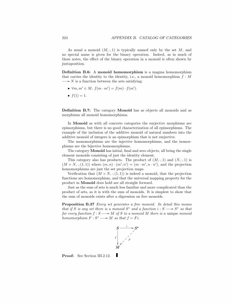
224 APPENDIX B. CATALOG OF CATEGORIES
As usual a monoid (M, ·, 1) is typically named only by the set M , andno special name is given for the binary operation. Indeed, as in much ofthese notes, the effect of the binary operation in a monoid is often shown byjuxtaposition.
Definition B.6: A monoid homomorphism is a magma homomorphismthat carries the identity to the identity, i.e., a monoid homomorphism f : M
// N is a function between the sets satisfying:
• ∀m,m′ ∈M, f(m ·m′) = f(m) · f(m′).
• f(1) = 1.
Definition B.7: The category Monoid has as objects all monoids and asmorphisms all monoid homomorphisms.
In Monoid as with all concrete categories the surjective morphisms areepimorphisms, but there is no good characterization of all epimorphisms. Theexample of the inclusion of the additive monoid of natural numbers into theadditive monoid of integers is an epimorphism that is not surjective.
The monomorphisms are the injective homomorphisms, and the isomor-phisms are the bijective homomorphisms.
The category Monoid has initial, final and zero objects, all being the singleelement monoids consisting of just the identity element.
This category also has products. The product of (M, ·, 1) and (N, ·, 1) is(M × N, ·, (1, 1)) where (m,n) · (m′, n′) = (m ·m′, n · n′), and the projectionhomomorphisms are just the set projection maps.
Verification that (M ×N, ·, (1, 1)) is indeed a monoid, that the projectionfunctions are homomorphism, and that the universal mapping property for theproduct in Monoid does hold are all straight forward.
Just as the sum of sets is much less familiar and more complicated than theproduct of sets, so it is with the sum of monoids. It is simplest to show thatthe sum of monoids exists after a digression on free monoids.
Proposition B.37 Every set generates a free monoid. In detail this meansthat if S is any set there is a monoid S∗ and a function i : S // S∗ so thatfor every function f : S // M of S to a monoid M there is a unique monoidhomomorphism F : S∗ // M so that f = Fi.
S S∗i //S
M
f
S∗
M
F
Proof: See Section III.2.12.
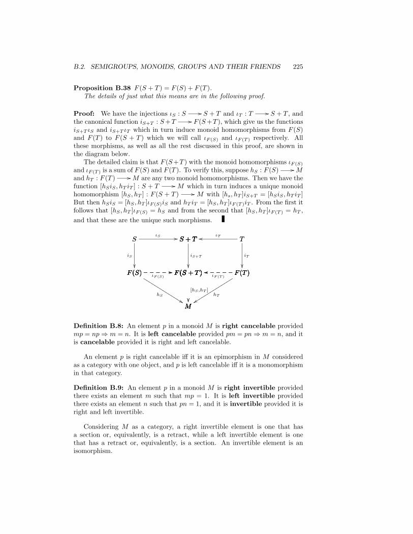
B.2. SEMIGROUPS, MONOIDS, GROUPS AND THEIR FRIENDS 225
Proposition B.38 F (S + T ) = F (S) + F (T ).The details of just what this means are in the following proof.
Proof: We have the injections ιS : S // S + T and ιT : T // S + T , andthe canonical function iS+T : S+T // F (S+T ), which give us the functionsiS+T ιS and iS+T ιT which in turn induce monoid homomorphisms from F (S)and F (T ) to F (S + T ) which we will call ιF (S) and ιF (T ) respectively. Allthese morphisms, as well as all the rest discussed in this proof, are shown inthe diagram below.
The detailed claim is that F (S+T ) with the monoid homomorphisms ιF (S)
and ιF (T ) is a sum of F (S) and F (T ). To verify this, suppose hS : F (S) // Mand hT : F (T ) // M are any two monoid homomorphisms. Then we have thefunction [hSiS , hT iT ] : S + T // M which in turn induces a unique monoidhomomorphism [hS , hT ] : F (S + T ) // M with [hs, hT ]iS+T = [hSiS , hT iT ]But then hSiS = [hS , hT ]ιF (S)iS and hT iT = [hS , hT ]ιF (T )iT . From the first itfollows that [hS , hT ]ιF (S) = hS and from the second that [hS , hT ]ιF (T ) = hT ,and that these are the unique such morphisms.
F (S) F (S + T )ιF (S)//_____
S
F (S)
iS
S S + TιS // S + T
F (S + T )
iS+T
F (S + T ) F (T )oo
ιF (T )_____
S + T
F (S + T )
S + T
F (S + T )
S + T Too ιTT
F (T )
iT
F (S) F (S + T )//_____F (S)
M
hS
%%KKKKKKKKKKKKKKF (S + T )
M
[hS ,hT ]
F (S + T ) F (T )oo _____F (S + T )
M
F (T )
M
hT
yyssssssssssssss
Definition B.8: An element p in a monoid M is right cancelable providedmp = np⇒ m = n. It is left cancelable provided pm = pn⇒ m = n, and itis cancelable provided it is right and left cancelable.
An element p is right cancelable iff it is an epimorphism in M consideredas a category with one object, and p is left cancelable iff it is a monomorphismin that category.
Definition B.9: An element p in a monoid M is right invertible providedthere exists an element m such that mp = 1. It is left invertible providedthere exists an element n such that pn = 1, and it is invertible provided it isright and left invertible.
Considering M as a category, a right invertible element is one that hasa section or, equivalently, is a retract, while a left invertible element is onethat has a retract or, equivalently, is a section. An invertible element is anisomorphism.

226 APPENDIX B. CATALOG OF CATEGORIES
Suppose have monoid M and monoid homomorphism h : M // U . LetS = s ∈M : h(s) is invertible . Then S is a submonoid.
Theorem B.19 For any subset S of a monoid M there is a monoid S−1Mand a monoid homomorphism h : M // S−1M with the following UniversalMapping Property:
1. ∀s ∈ S, h(s) is invertible in S−1M .
2. If f : M // N is a monoid homomorphism with f(s) invertible forall s ∈ S, then there exists a unique monoid homomorphism f : S−1M
// N with f = fh.
Corollary 2 For every monoid N there is a group Z and a monoid homo-morphism i : N // Z with the universal mapping property that for everymonoid homomorphism h : N // G of N to a group G there is a uniquegroup homomorphism H : Z // G so that h = Hi.
N Zi //N
G
h
Z
G
H
B.2.4 CMonoid – commutative monoids
Definition B.10: A commutative monoid is a monoid in which the oper-ation is commutative.
Definition B.11: CMonoid is the full subcategory of Monoid whose objectsare the commutative monoids.
In CMonoid the epimorphisms are the surjective homomorphisms, themonomorphisms are the injective homomorphisms, and the isomorphisms arethe bijective homomorphisms.
The category CMonoid has initial, final and zero objects, all being thesingle element monoids consisting of just the identity element.
This category also has products. The product of (M, ·, 1) and (N, ·, 1) is(M × N, ·, (1, 1) where (m,n) · (m′, n′) = (m · m′, n · n′), and the projectionhomomorphisms are just the set projection maps.
Verification that (M ×N, ·, (1, 1)) is indeed a monoid, that the projectionfunctions are homomorphism, and that the universal mapping property for theproduct in CMonoid does hold are all straight forward.
Just as the sum of sets is much less familiar and more complicated than theproduct of sets, so it is with the sum of commutative monoids.

B.2. SEMIGROUPS, MONOIDS, GROUPS AND THEIR FRIENDS 227
Proposition B.39 For every commutative monoid N there is an Abeliangroup Z and a monoid homomorphism i : N // Z so that for every monoidhomomorphism h : M // A of M to an Abelian group A there is a uniquegroup homomorphism H : Z // M so that h = Hi.
N Zi //N
A
h
Z
A
H
Proof: The construction of Z is based on the intuition that the elementsof Z arise as differences of elements of N . Moreover n′ − n = m′ −m whenn′ + m = n + m′, so define Z = N × N/ ∼ where (n′, n) ∼ (m′,m) whenn′+m = n+m′ and i(n) is the equivalence class of (n, 0) which we will denotefor the duration of this proof as ((n′, n)). The binary operation on Z is definedin the usual way: ((n′, n)) + ((m′,m)) = ((n′ + m′, n + m)) and this is well-defined, i.e., not dependent of the particular representatives. Straight forwardcomputations show that Z is an Abelian group with ((0, 0)) as identity and theinverse of ((n′, n)) is ((n, n′)).
Finally given the homomorphism h : N // A, if there is a group homo-morphism H : Z // A with Hi = h, then because ((n′, n)) = i(n′) − i(n)it follows that H((n′, n)) = h(n′) − h(n). Taking that as a definition, simplecomputations show that H is a well-defined group homomorphism with Hi = hand this guarantees uniqueness as well as existence.
Of course this is an example of a universal arrow (see Section V.2) fromthe commutative monoid N to the forgetful functor from the category Ab ofAbelian groups to the category of commutative monoids.
B.2.5 Group – groups
Definition B.12: A group is a monoid in which every element has an inverse.
Definition B.13: A group homomorphism is just a monoid homomor-phism.
It is natural to expect a requirement that a group homomorphism carriesinverses to inverses, but that is a formal consequence.
Definition B.14: The category Group has as objects all groups and asmorphisms the group homomorphisms between them.

228 APPENDIX B. CATALOG OF CATEGORIES
B.2.6 FiniteGroup – finite groups
The category FiniteGroup has as objects all groups and as morphisms thegroup homomorphisms between them.
B.2.7 Ab – Abelian groups
Definition B.15: An Abelian group (also called a commutative group) is agroup in which the binary operation is commutative.
The category Ab has as objects all Abelian groups and as morphisms thegroup homomorphisms between them.
B.2.7.1 TorAb – Torsion Abelian groups
B.2.7.2 DivAb – Divisible Abelian groups
B.2.7.3 TorsionFreeAb – Torsion Free Abelian groups
B.3 Rings
Rings are algebraic gadgets which have two binary operations, addition andmultiplication, that are connected in some approximation of the familiar sit-uation with numbers. The most common type of ring is sometimes called anassociative ring with identity, but here the name ring is reserved for this type.
Definition B.16: A ring is a set R equipped with two binary operations +and ·, called addition and multiplication, and distinguished elements 0 and 1such that:
• (R,+, 0) is an Abelian group:
∀a, b, c ∈ R
– 0 + a = a = a+ 0
– (a+ b) + c = a+ (b+ c)
– a+ b = b+ a
– For each a ∈ R there is an element −a such that a+−a = 0 = −a+a
• (R, ·, 1) is a monoid:
– (a · 1) = a = 1 · a– (a · b) · c = a · (b · c)
• Multiplication distributes over addition:
– a · (b+ c) = (a · b) + (a · c)– (a+ b) · c = (a · c) + (b · c)

B.3. RINGS 229
As with groups the symbol · is usually omitted and multiplication is justdenoted by juxtaposition. Also the standard order of operation rules are used,so that, for example, a+ bc is an abbreviation for a+ (b · c).
Although addition in a ring is commutative (i.e. a+ b = b+ a), multiplica-tion is not assumed to be commutative. Rings in which multiplication is alsocommutative (such as the ring of integers) are called commutative rings.
The category Ring of rings is discussed in Section B.3.3 below while itssubcategory of commutative rings is discussed in Section B.3.4.
There are a wide variety of interesting generalizations, most of them gottenby eliminating one or more of the items in the above definition. For examplerngs are rings without identity. Here is the actual definition.
Definition B.17: A rng is a set R equipped with two binary operations +and ·, called addition and multiplication, and a distinguished element 0 suchthat:
• (R,+, 0) is an Abelian group.
• (R, ·) is a semigroup.
• Multiplication distributes over addition.
The category Rng of rings without identity is discussed in Section B.3.2.Contrary to what the name suggests a rng may have a multiplicative identity,in particular every ring is a rng.
The simplest examples of rngs are gotten by defining multiplication on anyAbelian group (A,+, 0) by a · b = 0 for all a, and b in A. The only case whenthis has an identity is the zero ring which has only one element, 0.
The system (N,+, 0, ·, 1) satisfies almost all of the condition to be a com-mutative ring – the only thing missing are negative numbers. Such gadgets arecalled rigs (“rings without negatives”) or semirings and defined as follows.
Definition B.18: A rig is a set R equipped with two binary operations +and ·, called addition and multiplication, and distinguished element 0 and 1such that:
• (R,+, 0) is a commutative monoid.
• (R, ·, 1) is a monoid.
• Multiplication distributes over addition.
A particularly interesting class is the non-associative rings (remove the as-sumption that multiplication is associative) and various specific variations suchas Lie rings and Jordan rings (which replace the associative law with a partic-ular alternative).
Another direction is the class of rings called algebras. These are rings ofone or another of the various types already mentioned but where the additive

230 APPENDIX B. CATALOG OF CATEGORIES
Abelian group is assumed to be a vector space over some field or, more generally,a module over some base ring. A variety of categories of algebras are discussedin Section B.5.
B.3.1 Rig – rings without negatives
Recall that rigs were defined back in Section B.3.3 as follows.A rig is a set R equipped with two binary operations + and ·, called addition
and multiplication, and distinguished elements 0 and 1 such that:
• (R,+, 0) is an commutative monoid group.
• (R, ·, 1) is a monoid.
• Multiplication distributes over addition.
Examples
• The most familiar example of a rig that is not a ring is N with the usualaddition and multiplication.
• If R is any rig and X is any non-empty set, then the set RX of allfunctions from X to R is a rig – the operations in RX come from pointwiseoperations: (f + g)(x) = f(x) + g(x), (fg)(x) = f(x)g(x), 0(x) = 0, and1(x) - 1.
Definition B.19: A rig homomorphism is a function from one rig to an-other which is a group homomorphism between the additive monoids and asemigroup homomorphism between the multiplicative semigroups.
In detail a rig homomorphism f : R // S satisfies:
(i) f(0) = 0.
(ii) f(r + r′) = f(r) + f(r′).
(iii) f(1) = 1.
(iv) f(r · r′) = f(r) · f(r′).
Definition B.20: The category Rig has as object all rigs (as defined above)and as morphisms all rig homomorphisms.
The identity function on a rig is a rig homomorphism, and the functioncomposition of two rig homomorphism is again a rig homomorphism. Withthose two observations it is a now familiar formality to verify that Rig isindeed a category.
Theorem B.20 Given a rig (R,+, 0, ·, 1), there is a universal morphism fromR to a ring.

B.3. RINGS 231
Proof: On R × R define (a, b) (c, d) <=> ∃z ∈ R, a + d + z = c + b + z.The quotient R(R) = (RR)/ is a ring and the map R // R(R) given byx 7→ [(x, 0)]/ “(= ”x - 0”)” is a rig morphism. In general, the morphism R
// R(R) need not be injective.
B.3.2 Rng – rings without identity
Definition B.21: A rng homomorphism is a function from one rng toanother which is a group homomorphism between the additive groups and alsoa semigroup homomorphism between the multiplicative semigroups.
In detail a rng homomorphism f : R // S satisfies:
(i) f(0) = 0.
(ii) f(r + r′) = f(r) + f(r′).
(iii) f(r · r′) = f(r) · f(r′).
The identity function on a rng is a rng homomorphism, and the functioncomposition of two rng homomorphism is again a rng homomorphism. Withthose two observations it is a now familiar formality to verify that Rng isindeed a category.
B.3.3 Ring – associative rings with identity
As with groups the symbol × is usually omitted and multiplication is justdenoted by juxtaposition. Also the standard order of operation rules are used,so that, for example, a+ bc is an abbreviation for a+ (b× c).
Although ring addition is commutative (i.e. a + b = b + a), note thatthe commutativity for multiplication (a × b = b × a) is not among the ringaxioms listed above. Rings that also satisfy commutativity for multiplication(such as the ring of integers) are called commutative rings. Not all rings arecommutative.
Definition B.22: A ring homomorphism is just an rng homomorphism.In detail a ring homomorphism f : R // S satisfies:
(i) f(0) = 0.
(ii) f(r + r′) = f(r) + f(r′).
(iii) f(1) = 1.
(iv) f(r · r′) = f(r) · f(r′).
The identity function on a ring is a ring homomorphism, and the functioncomposition of two ring homomorphism is again a ring homomorphism. With

232 APPENDIX B. CATALOG OF CATEGORIES
those two observations it is a now familiar formality to verify that Ring isindeed a category.
B.3.4 CommutativeRing – commutative rings
CommutativeRing is the category of commutative rings with identity withmorphisms being the rings homomorphisms (which take 1 to 1.)
B.3.5 Field – fields
Definition B.23: A field is a commutative ring in which every non-zeroelement has a multiplicative inverse.
B.4 Modules
B.4.1 Module – modules over a commutative ring
Throughout this section R is a commutative ring.
Definition B.24: An R-module M is an Abelian group (M,+, 0) togetherwith a function R×M // M (written as (r,m) 7→ rm) satisfying: For all m,n in M and for all r, s in R
(i) r(m + n) = rm + rn.
(ii) 1m = m.
(iii) (r + s)m = rm + sm.
(iv) (rs)m = r(sm).
This is actually a family of categories. For each commutative ring R thereis the category ModuleR with objects all R-modules and morphisms all R-module homomorphisms. In the case that R = Z, the category ModuleZ is thesame as Ab. As you should expect there is in general a great deal of similaritybetween Ab and other categories of modules.
Much of the time the particular ring is not interesting, in which caseModule will be written to stand for ModuleR with R unspecified.
B.4.2 Matrices – matrices over a commutative ring
This is another parametrised family of categories. For each commutative ringR, the category MatricesR has as objects all positive integers and as mor-phisms matrices with entries in R. In particular an m×n matrix is a morphismfrom n to m with the identity morphism on m being the m×m identity matrix,and composition being the usual matrix multiplication.

B.5. ALGEBRAS 233
This category is actually equivalent to the full subcategory of all finitelygenerated free R-modules in ModuleR.
B.4.3 Vect – vector spaces
For each field K we have the category VectK which has as objects all vectorspaces over K and as morphisms all linear transformations between them. Thisis really just the category ModuleK , but it is sufficiently interesting and wellstudied in its own right that we will treat it separately.
Much of the time the particular field is not interesting, in which case Vectwill be written to stand for VectK with K unspecified.
B.4.4 FDVect – finite dimensional vector spaces
The full subcategory FDVectK of FDVectK has as objects just the finitedimensional vector spaces in VectK . This is is sufficiently interesting that itdeserves separate mention.
Much of the time the particular field is not interesting, in which caseFDVect will be written to stand for FDVectK with K unspecified.
B.5 Algebras
Algebras are rings in which the additive structure is not just an Abelian group,but a module over a commutative ring. The most commonly discussed algebrasare associative algebras over fields, but here we will reserve the name algebrafor associative algebras over a commutative ring.
Throughout this section R will be a commutative ring.
Definition B.25: An R-algebra is both an R-module and a ring in such a waythat multiplication in the ring is an R-bilinear map. In detail an R-algebra
B.5.1 Algebra – associative algebras
This is actually a family of categories. For a fixed commutative ring (with iden-tity), R, AlgebraR is the category with objects all R-algebras and morphismsall the algebra homomorphisms. By an algebra we certainly mean a set withboth an operation of addition and an operation of multiplication. Moreovereach ring is an Abelian group with respect to addition.
And we require the algebra homomorphisms to take 1 to 1.Much of the time the particular commutative ring is not interesting, in
which case Algebra will be written to stand for AlgebraR with R unspecified.
B.5.2 LieAlgebra – Lie algebras
This is actually a family of categories. For a fixed commutative ring (withidentity), R, LieAlgebra is the category with objects all R Lie algebras and

234 APPENDIX B. CATALOG OF CATEGORIES
morphisms all the Lie algebra homomorphisms.
B.6 Order
B.6.1 Preorder – preorders
The category Preorder has as objects all preorders and as morphisms all theorder preserving functions between them.
As the identity function on any preorder is certainly order preserving andthe composition of two order preserving functions is also order preserving, wesee that Preorder is indeed a category.
Proposition B.40 The category Preorder has products.
Proof: For partially ordered sets X and Y define a partial order on productset X × Y by (x, y) ≤ (x′, y′) iff x ≤ x′ and y ≤ y′. The usual projectionfunctions πX and πY are certainly order preserving. Moreover if f : Z // Xand g : Z // Y are preorder morphisms, i.e., monotone functions, then thefunction (f, g) : Z // X × Y is monotone and clearly has the universalmapping property required for a product.
Proposition B.41 The category Preorder has sums.
B.6.2 Poset – partially ordered sets
Partially ordered sets, or posets, are those preorders where the order rela-tion is antisymmetric:
∀x, y ∈ X,x ≤ y ∧ y ≤ x⇒ x = y.
The category Poset of partially ordered sets is the full subcategory ofPreorder with objects the posets.
For more information about posets, consult Mac Lane and Birkhoff [55,II.8, IV.6, XIV].)
B.6.3 Lattice – lattices
The category Lattice has as objects all lattices and lattice morphisms betweenthem.
There are two quite different ways to describe lattices – as certain types ofpartially ordered sets, and as certain types of algebraic structures. We startwith the poset approach.
Lattices as posets In any poset L we have the notions of upper and lowerbounds and from them the notions least upper bounds and greatest lowerbounds, the essential notions for defining a lattice.

B.6. ORDER 235
Recall from definition A.56 that if S is any subset of a poset L, then u ∈ Lis an upper bound for S provided s ∈ S ⇒ s ≤ u.
Equally well there is the dual notion of a lower bound: l is a lower boundfor S provided s ∈ S ⇒ s ≥ l.
A least upper bound is a minimum among upper bounds, while a greatestlower bound is a maximum among lower bounds. The notion of glb is dual tothe notion of lub.
Now a lattice is a poset in which non-empty finite sets have lubs and glbs.
Definition B.26: A lattice is a poset in which every pair of elements hasboth a lub and a glb. The lub of x, y is called the join of x and y and iswritten as x ∨ y, while the glb of x, y is called the meet of x and y and iswritten as x ∧ y.
So every lattice, L, has binary operations ∧ : L × L // L and ∨ : L × L// L. The order relation can be retrieved from the meet and join: x ≤
y ⇐⇒ x ∧ y = y ∧ x ∨ y = x. This will be the connection between the orderand algebraic definitions.
The morphisms between lattices are not just order preserving, they arerequired to preserve meets and joins as well.
Definition B.27: A lattice morphism f : L // L′ is a function withf(x ∧ y) = f(x) ∧ f(y) and f(x ∨ y) = f(x) ∨ f(y).
While no requirement that a lattice morphism be order preserving wasexplicitly mentioned, the connection between the order relation and the meetsand joins guarantees that a lattice morphism is a poset morphism as well.
Although the definition of a lattice only requires the existence of lubs andglbs for two element sets, induction on the number of elements in a set easilyshows that lubs and glbs for all non-empty finite sets exists in every lattice.
For more information consult Mac Lane and Birkhoff [55, XIV].)It will be stated explicitly whenever a lattice is required to have a least or
greatest element. If both of these special elements do exist, then the poset iscalled a bounded lattice. An easy induction argument also shows the existenceof all suprema and infima of non-empty finite subsets of any lattice.
the above definition in terms of the existence of suitable Galois connectionsbetween related posets – an approach that is of special interest for categorytheoretic investigations of the concept.
Lattices as algebraic structuresConsider an algebraic structure in the sense of universal algebra, given by
(L,∨,∧), where ∨and ∧are two binary operations. L is a lattice if the followingidentities hold for all elements a, b, and c in L:
• Idempotent laws: a ∨ a = a, a ∧ a = a
• Commutative laws: a ∨ b = b ∨ a, a ∧ b = b ∧ a
• Associative laws: a ∨ (b ∨ c) = (a ∨ b) ∨ c, a ∧ (b ∧ c) = (a ∧ b) ∧ c

236 APPENDIX B. CATALOG OF CATEGORIES
• Absorption laws: a ∨ (a ∧ b) = a, a ∧ (a ∨ b) = a
It turns out that the idempotency laws can be deduced from absorptionand thus need not be stated separately.
Bounded lattices include neutral elements 0 and 1 for the meet and joinoperations in the above definition.
Connection between both definitionsObviously, an order theoretic lattice gives rise to two binary operations
∨and ∧. It now can be seen very easily that this operation really makes (L,∨,∧)a lattice in the algebraic sense. More surprisingly the converse of this resultis also true: consider any algebraically defined lattice (M,∨,∧). Now define apartial order ≤ on M by setting
x ≤ y iff x = x ∧ yor, equivalently,x ≤ y iff y = x ∨ yfor all elements x and y in M. The above laws for absorption ensure that
both definitions are indeed equivalent. An easy check shows that the relation≤ introduced in this way defines a partial ordering within which binary meetsand joins are given through the original operations ∨and ∧. Conversely, theorder induced by the algebraically defined lattice (L,∨,∧) that was derivedfrom the order theoretic formulation above coincides with the original orderingof L.
Hence, the two definitions can be used in an entirely interchangeable way,depending on which of them appears to be more convenient for a particularpurpose.
Examples
• For any set A, the collection of all finite subsets of A (including the emptyset) can be ordered via subset inclusion to obtain a lattice. The latticeoperations are intersection (meet) and union (join) of sets, respectively.This lattice has the empty set as least element, but it will only containa greatest element if A itself is finite. So it is not a bounded lattice ingeneral.
• The natural numbers in their common order are a lattice, the latticeoperations given by the min and max operations. The least element ofthis lattice is 0, but no greatest element exists.
• Any complete lattice (also see below) is a (rather specific) bounded lat-tice. A broad range of practically relevant examples belongs to this class.
• The set of compact elements of an arithmetic complete lattice is a latticewith a least element, where the lattice operations are given by restrictingthe respective operations of the arithmetic lattice. This is the specificproperty which distinguishes arithmetic lattices from algebraic lattices,for which the compacts do only form a join-semilattice. Both of theseclasses of complete lattices are studied in domain theory.

B.6. ORDER 237
Further examples are given for each of the additional properties that arediscussed below.
Morphisms of latticesThe appropriate notion of a morphism between two lattices can easily be
derived from the algebraic definition above: given two lattices (L,∨,∧) and(M,∪,∩), a homomorphism of lattices is a function f : L // M with theproperties that
• f(x ∨ y) = f(x) ∪ f(y), and
• f(x ∧ y) = f(x) ∩ f(y).
In the order-theoretical formulation, these conditions just state that a ho-momorphism of lattices is a function that preserves binary meets and joins. Forbounded lattices, preservation of least and greatest elements is just preservationof join and meet of the empty set.
Note that any homomorphism of lattices is necessarily monotone with re-spect to the associated ordering relation. For an explanation see the article onpreservation of limits. The converse is of course not true: monotonicity doesby no means imply the required preservation properties.
Using the standard definition of isomorphisms as invertible morphisms, onefinds that an isomorphism of lattices is exactly a bijective lattice homomor-phism. Lattices and their homomorphisms obviously form a category.
Properties of latticesThe definitions above already introduced the simple condition of being a
bounded lattice. A number of other important properties, many of which leadto interesting special classes of lattices, will be introduced below.
B.6.4 Full subcategories of equationally defined lattices
Complete Lattices Definition B.28: A lattice is complete provided allof its subsets has both a least upper bound and a greatest lower bound.
Distributive Lattices Since any lattice comes with two binary operations,it is natural to consider distributivity laws among them.
Definition B.29: A lattice (L,∨,∧) is distributive, provided x, y and z inL implies
x ∨ (y ∧ z) = (x ∨ y) ∧ (x ∨ z)
Surprisingly, this condition turns to be equivalent to its dual statement:
x ∧ (y ∨ z) = (x ∧ y) ∨ (x ∧ z)

238 APPENDIX B. CATALOG OF CATEGORIES
Modular Lattices Distributivity is too strong a condition for certain appli-cations. A strictly weaker but still useful property is modularity.
Definition B.30: A lattice (L,∨,∧) is modular provided x, y, and z in Limplies
x ∨ (y ∧ (x ∨ z)) = (x ∨ y) ∧ (x ∨ z)Another equivalent statement of this condition is as follows: if x ≤ z then
for all yx ∨ (y ∧ z) = (x ∨ y) ∧ z
For example, the lattice of submodules of a module and the lattice of normalsubgroups of a group have this special property. Furthermore, every distribu-tive lattice is indeed modular.
B.6.5 Boolean – the categories of Boolean algebras andBoolean rings
There are two apparently quite different notions – Boolean rings and Booleanalgebras – that have been recognized as “equivalent” for a long time. For bothof these notions we have categories and the categories are naturally equivalent.
Definition B.31: A Boolean ring is a ring (cf. Section B.3.3 on Ring) inwhich every element is idempotent, i.e., for every element b of a Boolean ringB we have b2 = b.
The canonical example of a Boolean ring is Z2, the integers modulo 2.The other basic example is the ring of subsets of a given set: For any set
X we have the set P(X) of all subsets of X (cf page 86.) Define the “sum” oftwo elements of P(X) to be their symmetric difference (cf 187)), i.e., S + T =(S − T ) ∪ (T − S) = (S ∪ T ) − (S ∩ T ) = x : x ∈ S ∨ x ∈ T but not bothand the product of two elements to be their intersection, i.e., S • T = S ∩ T .In fact if X is a one element set, then
A Boolean algebra is a lattice (A,∧,∨) (considered as an algebraic struc-ture) with the following four additional properties:
1. bounded below: ∃0 ∈ A ∀a ∈ A a ∨ 0 = a.
2. bounded above: ∃1 ∈ A ∀a ∈ A a ∧ 1 = a.
3. distributive law: ∀a, b, c ∈ A(a ∨ b) ∧ c = (a ∧ c) ∨ (b ∧ c).
4. existence of complements: ∀a ∈ A ∃¬a ∈ A (a ∨ ¬a = 1 ∧ a ∧ ¬a = 0).
From these axioms, we find that the smallest element 0, the largest element 1,and the complement ¬a of any element a are uniquely determined.
Like any lattice, a Boolean algebra (A,∧,∨) gives rise to a partially orderedset (A,≤ ) by defining a ≤ b iff a = a∧ b (which is also equivalent to b = a∨ b).

B.6. ORDER 239
Equally well a Boolean algebra can be defined as distributive lattice (A,≤)(considered as a partially ordered set) with least element 0 and greatest element1, within which every element x has a complement ¬x such that x ∧ ¬x = 0and x ∨ ¬x = 1.
Here ∧ and ∨ are used to denote the infimum (meet) and supremum (join)of two elements. Again, if complements in the above sense exist, then they areuniquely determined.
The algebraic and the order theoretic perspective as usual can be used in-terchangeably and both are of great use to import results and concepts fromboth universal algebra and order theory. In many practical examples an order-ing relation, conjunction, disjunction, and negation are all naturally available,so that it is straightforward to exploit this relationships.
Here are several other theorems valid in all Boolean algebras. For example,for all elements a and b of a Boolean algebra, a ∧ 0 = 0 and a ∨ 1 = 1,¬1 = 0 and ¬0 = 1, ¬¬a = a and that both de Morgan’s laws are valid, i.e.¬(a ∧ b) = (¬a) ∨ (¬b) and ¬(a ∨ b) = (¬a) ∧ (¬b).
General insights from duality in order theory apply to Boolean algebras.Especially, the order dual of every Boolean algebra, or, equivalently, the algebraobtained by exchanging ∧ and ∨, is also a Boolean algebra. Thus the dualversion of the distributive law, (a ∧ b) ∨ c = (a ∨ c) ∧ (b ∨ c) also holds true.In general, any law valid for Boolean algebras can be transformed into anothervalid dual law by exchanging 0 with 1, ∧ with ∨, and ≤ with ≥.
A homomorphism between the Boolean algebras A and B is a functionf : A // B such that ∀a ∈ A ∀b ∈ A , f(a ∧ b) = f(a) ∧ f(b) and f(a ∨ b) =f(a) ∨ f(b) and f(0) = 0, f(1) = 1.
It then follows that f(¬a) = ¬f(a) for all a ∈ A as well. The class of allBoolean algebras, together with this notion of morphism, forms a category. Anisomorphism from A to B is a homomorphism from A to B which is bijective.The inverse of an isomorphism is also an isomorphism, and we call the twoBoolean algebras A and B isomorphic. From the standpoint of Boolean algebratheory, they cannot be distinguished; they only differ in the notation of theirelements.
Boolean rings, ideals and filtersEvery Boolean algebra (A,∧,∨) gives rise to a ring (A,+, ∗) by defining
a+b = (a∧¬b)∨(b∧¬a) (this operation is called ”symmetric difference” in thecase of sets and XOR in the case of logic) and a∗b = a∧b. The zero element ofthis ring coincides with the 0 of the Boolean algebra; the multiplicative identityelement of the ring is the 1 of the Boolean algebra. This ring has the propertythat a ∗ a = a for all a ∈ A; rings with this property are called Boolean rings.
Conversely, if a Boolean ring A is given, we can turn it into a Booleanalgebra by defining x ∨ y = x + y − xy and x ∧ y = xy. Since these twooperations are inverses of each other, we can say that every Boolean ring arisesfrom a Boolean algebra, and vice versa. Furthermore, a map f : A // Bis a homomorphism of Boolean algebras if and only if it is a homomorphismof Boolean rings. The categories of Boolean rings and Boolean algebras areequivalent.

240 APPENDIX B. CATALOG OF CATEGORIES
An ideal of the Boolean algebra A is a subset I such that for all x, y ∈ Iwe have x ∧ y ∈ I and for all a ∈ A we have a ∧ x ∈ I. This notion of idealcoincides with the notion of ring ideal in the Boolean ring A. An ideal I of Ais called prime if I 6= A and if a∧b ∈ I always implies a ∈ I or b ∈ I. An idealI of A is called maximal if I 6= A and if the only ideal properly containing Iis A itself. These notions coincide with ring theoretic ones of prime ideal andmaximal ideal in the Boolean ring A.
The dual of an ideal is a filter. A filter of the Boolean algebra A is a subsetp such that for all x, y ∈ p we have x∧ y ∈ p and for all a ∈ A if a∨x = a thena ∈ p.
A Boolean algebra (Boolean algebra) is a set A together with binary op-erations + and × and a unary operation -, and elements 0, 1 of A such thatthe following laws hold: commutative and associative laws for addition andmultiplication, distributive laws both for multiplication over addition and foraddition over multiplication, and the following special laws:
• x+ (x× y) = x
• x× (x+ y) = x
• x+ (−x) = 1
• x× (−x) = 0
These laws are better understood in terms of the basic example of a Booleanalgebra, consisting of a collection A of subsets of a set X closed under theoperations of union, intersection, complementation with respect to X, withmembers ∅ and X. Many elementary laws follow from these axioms, keepingin mind this example for motivation. Any Boolean algebra has a natural par-tial order ≤ defined upon it by saying that x ≤ y if and only if x + y = y.This corresponds in our main example to ⊆. Of special importance is the two-element Boolean algebra, formed by taking the set X to have just one element.An important elementary result is that an equation holds in all Boolean al-gebras if and only if it holds in the two-element Boolean algebra. Next, wedefine x ⊕ y = (x − y) + (y − x). Then A together with ⊕ and ×, alongwith 0 and 1, forms a ring with identity in which every element is idempotent.Conversely, given such a ring, with addition ⊕ and multiplication ×, definex + y = x⊕ y ⊕ (x× y) and −x = 1⊕ x. This makes the ring into a Booleanalgebra. These two processes are inverses of one another, and show that thetheory of Boolean algebras and of rings with identity in which every elementis idempotent are definitionally equivalent. This puts the theory of Booleanalgebras into a standard object of research in algebra.
An atom in a Boolean algebra is a nonzero element a such that there isno element b with 0 < b < a. A Boolean algebra is atomic if every nonzeroelement of the Boolean algebra is above an atom. Finite Boolean algebras areatomic, but so are many infinite Boolean algebras. Under the partial order ≤above, x+y is the least upper bound of x and y, and x×y is the greatest lowerbound of x and y. We can generalize this: ΣX is the least upper bound of a

B.6. ORDER 241
set X of elements, and ΠX is the greatest lower bound of a set X of elements.These do not exist for all sets in all Boolean algebras; if they do always exist,the Boolean algebra is said to be complete.
2. The elementary algebraic theorySeveral algebraic constructions have obvious definitions and simple prop-
erties for Boolean algebras: subalgebras, homomorphisms, isomorphisms, anddirect products (even of infinitely many algebras). Some other standard al-gebraic constructions are more peculiar to Boolean algebras. An ideal ina Boolean algebra is a subset I closed under +, with 0 as a member, andsuch that if a ≤ b ∈ I, then also a ∈ I. Although not immediately obvi-ous, this is the same as the ring-theoretic concept. There is a dual notionof a filter (with no counterpart in rings in general). A filter is a subset Fclosed under × , having 1 as a member, and such that if a ≥ b ∈ F , thenalso a ∈ F . An ultrafilter on A is a filter F with the following properties:0 /∈ F , and for any a ∈ A, either a ∈ F or −a ∈ F . For any a ∈ A, letS(a) = F : F is an ultrafilter on A∧ a ∈ F. Then S is an isomorphism ontoa Boolean algebra of subsets of the setX of all ultrafilters on A. This establishesthe basic Stone representation theorem, and clarifies the origin of Boolean alge-bras as concrete algebras of sets. Moreover, the sets S(a) can be declared to bea base for a topology on X, and this turns X into a totally disconnected com-pact Hausdorff space. This establishes a one-to-one correspondence betweenthe class of Boolean algebras and the class of such spaces. As a consequence,used very much in the theory of Boolean algebras, many topological theoremsand concepts have consequences for Boolean algebras. If x is an element ofa Boolean algebra, we let 0x = −x and 1x = x. If (x(0), . . . , x(m − 1)) is afinite sequence of elements of a Boolean algebra A, then every element of thesubalgebra of A generated by x(0), . . . , x(m− 1) can be written as a sum ofmonomials e(0)x(0) × · · · × e(m − 1)x(m − 1) for e in some set of functionsmapping m = 0, . . . ,m − 1 into 2 = 0, 1. This is an algebraic expressionof the disjunctive normal form theorem of sentential logic. A function f froma set X of generators of a Boolean algebra A into a Boolean algebra B can beextended to a homomorphism if and only if e(0)x(0) . . . e(m− 1)x(m− 1) = 0always implies that e(0)f(x(0)) . . . e(m− 1)f(x(m− 1)) = 0. This is Sikorski’sextension criterion. Every Boolean algebra A can be embedded in a completeBoolean algebra B in such a way that every element of B is the least upperbound of a set of elements of A. B is unique up to A-isomorphism, and iscalled the completion of A. If f is a homomorphism from a Boolean algebraA into a complete Boolean algebra B, and if A is a subalgebra of C, then fcan be extended to a homomorphism of C into B. This is Sikorski’s extensiontheorem. Another general algebraic notion which applies to Boolean algebrasis the notion of a free algebra. This can be concretely constructed for Booleanalgebras. Namely, the free Boolean algebra on K is the Boolean algebra ofclosed-open subsets of the two element discrete space raised to the K power.

242 APPENDIX B. CATALOG OF CATEGORIES
B.6.5.1 Boolean – the category of complete Boolean algebras
B.7 Ordered Algebraic Structures
B.7.1 OrderedMagma – Ordered Magmas
An ordered magma is both a magma and a poset where the order is respectedby the binary operation of the magma.
Definition B.32: An ordered magma is a magma (M, ·) which also has apartial order ≤ with the property:
∀m,n, p ∈M [m ≤ n⇒ mp ≤ np ∧ pm ≤ pn]
The basic example of an ordered magma is the additive magma of naturalnumbers with the usual ordering. In this case the defining property connectingthe order with addition reads:
∀m,n, p ∈ N [m ≤ n⇒ m+ p ≤ n+ p ∧ p+m ≤ p+ n]
The multiplicative magma of natural numbers with the usual ordering isanother quite different ordered magma where we have the familiar property:
∀m,n, p ∈ N [m ≤ n⇒ mp ≤ np ∧ pm ≤ pn]
B.7.2 OrderedMonoid – Ordered Monoids
Definition B.33: An ordered monoid is a monoid (M, 1, ·) which also hasa partial order ≤ with the property:
∀m,n, p ∈M [m ≤ n⇒ mp ≤ np ∧ pm ≤ pn]
The basic example of an ordered monoid is the additive monoid of naturalnumbers with the usual ordering. In this case the defining property connectingthe order with addition reads:
∀m,n, p ∈ N [m ≤ n⇒ m+ p ≤ n+ p ∧ p+m ≤ p+ n]
The multiplicative monoid of natural numbers with the usual ordering isanother quite different ordered monoid.
B.7.3 OrderedGroup – Ordered Groups
Definition B.34: An ordered group is an ordered monoid in which everyelement has an inverse.

B.7. ORDERED ALGEBRAIC STRUCTURES 243
By contrast with an ordered monoid the order relation can be reduced tocomparison with the identity: g ≤ h iff 1 ≤ g−1h which is also equivalent to1 ≤ hg−1. This can be carried a step further and the order specified in terms ofan invariant subset. When G is an ordered group, define G+ = g ∈ G : 1 ≤ g.Then G+ has three characteristic properties:
(i) 1 ∈ G+.
(ii) g, h ∈ G+ ⇒ gh ∈ G+.
(iii) ∀g ∈ G [h ∈ G+ ⇒ g−1hg ∈ G+.
In the reverse direction, if G+ is a subset of a group G and has the above threeproperties, then defining g ≤ h iff g−1h ∈ G+ makes ≤ a partial order on G insuch a way that it is an ordered group.
The basic example of an ordered group is the additive group of integerswith the usual ordering.
B.7.4 OrderedRig – Ordered Rigs
Definition B.35: An ordered rig is a rig R together with a partial order,≤, which is an ordered monoid under addition and ∀r, s, t ∈ R, r ≤ s ∧ 0 ≤t⇒ rt ≤ st ∧ tr ≤ ts.
Examples
• The most familiar example of an ordered rig is N with all the usualstructure.
• Every rig is an ordered rig for the trivial partial order where a ≤ b iffa = b.
• If R is any rig and X is any non-empty set, then the set RX of allfunctions from X to R is a rig (see Section B.3.1) and is an ordered rigfor the partial order f ≤ g ⇐⇒ ∀x ∈ X, f(x) ≤ g(x).
Definition B.36: A homomorphism of ordered rigs is a rig homomor-phism that is also a monotone function between the two partially ordered sets.
Definition B.37: The category OrderedRig of ordered rigs has as objectsall ordered rigs and as morphisms the homomorphisms between them.
The identity function on an ordered rig is a homomorphism of ordered rigs,and the function composition of two homomorphisms of ordered rigs is again ahomomorphism of ordered rigs, so it is a now familiar formality to verify thatOrderedRig is indeed a category.

244 APPENDIX B. CATALOG OF CATEGORIES
Proposition B.42 For every ordered commutative rig R there is an orderedcommutative ring S and a universal ordered rig homomorphism i : R // S,i.e., if h : R // T is an ordered rig homomorphism to an ordered ring T ,then there is a unique ordered ring homomorphism h : S // T with hi = h
Proof: There is an easy construction based on the perception that the ele-ments of S are differences of elements of R.
Let S′ = R × R and define the relation on S′ by (r1, r2) (r′1, r′2) iff there
is some r′′ ∈ R such that
B.7.5 OrderedRing – Ordered Rings
Throughout this section only non-zero rings will be considered. This is thesame as saying that 0 6= 1 in all of these rings.
Definition B.38: A compatible order on a ring R is a subset R+ of Rsatisfying: ∀r, s ∈ R ,
(i) r, s ∈ R+ ⇒ r + s ∈ R+ ∧ rs ∈ R+.
(ii) (Trichotomy Law) If r 6= 0, then either r ∈ R+ or −r ∈ R+, but notboth.
An ordered ring is a non-zero ring together with a compatible order.
B.8 Graphs
B.8.1 Graph – graphs
The category Graph has as objects all graphs and graph homomorphismsbetween them.
Definition B.39: A graph is a pair of sets G = (V , E) with each elementof E a 2-element subset of V . The elements of V are called the verticesof G,and the elements of E are called the edgesof G.
A good introductory treatment of graph theory is Diestel [14]. Of course thecategory of graphs must have morphisms, but like most texts on graph theoryDiesel makes no mention of graph homomorphism (though isomorphisms andcolorings appear), and graph are assumed finite. Graph homomorphisms haveactually been studied for 50 years or so, but there are only a couple of booksthat discuss them in any depth, for example see Hell and Nesetril [31] whichis however almost exclusively about finite graphs.
Definition B.40:

B.9. TOPOLOGY 245
B.8.2 Digraph – directed graphs
The category Digraph has as objects all directed graphs (commonly calleddigraphs) and digraph homomorphisms between them.
Definition B.41:
Definition B.42:
B.9 Topology
B.9.1 Metric – metric spaces
The category Metric has as objects all metric spaces and as morphisms allcontractions between them. [RIGHT CHOICE?]
B.9.2 Uniform – uniform spaces
The category Uniform has as objects all uniform spaces and as morphisms alluniformly continuous functions between them.
B.9.3 Top – topological spaces
The category Top has as objects all topological spaces and as morphisms allcontinuous functions between them.
B.9.4 Comp – compact Hausdorff spaces
The category Comp has as objects all compact Hausdoff topological spacesand as morphisms all continuous functions between them.
B.9.5 Kspace – K-spaces
The category Kspace has as objects all compactly generated Hausdorff topo-logical spaces (K-spaces) and as morphisms all continuous functions betweenthem.
B.9.6 Homotopy – the homotopy category of topologicalspaces
Homotopy is the quotient category of Top where the equivalence relationon continuous functions is homotopy, i.e., for f0, f1 : X // Y , f0 ' f1 iffthere exists a continuous functions (a “homotopy”) F : X × [0, 1] // Y withF (x, 0) = f0(x) and F (x, 1) = f1(x) for all x ∈ X.

246 APPENDIX B. CATALOG OF CATEGORIES
B.9.7 HSpace – H-Spaces
HSpace are
B.10 Simplicial Categories
B.10.1 Simplicial – simplicial sets
The category of simplicial sets has as objects all simplicial sets and as mor-phisms ...
Let C be a small category. It is easy to define the sets N(C )k for smallk, which leads to the general definition. In particular, there is a 0-simplex ofN(C ) for each object of C . There is a 1-simplex for each morphism f : x
// y in C . Now suppose that f : x // y and g : y // z are morphisms inC . Then we also have their composition gf : x // z.
A 2-simplex.
A
Bf
??A
C
gf
????????
The diagram suggests our course of action: add a 2-simplex for this com-mutative triangle. Every 2-simplex of N(C ) comes from a pair of composablemorphisms in this way. Note that the addition of these 2-simplices does noterase or otherwise disregard morphisms obtained by composition, it merelyremembers that that is how they arise.
In general, N(C )k consists of the k-tuples of composable morphismsA0
// A1// A2
// · · · // Ak−1// Ak
of C . To complete the definition of N(C ) as a simplicial set, we must alsospecify the face and degeneracy maps. These are also provided to us by thestructure of C as a category. The face maps
di : N(C )k // N(C )k−1
are given by composition of morphisms at the i-th object. This means thatdi sends the k-tuple
A0// A1
// A2// · · · // Ak−1
// Akto the (k-1)-tupleA0
// · · ·Ai−1// Ai+1
// · · · // Ak .That is, the map di composes the morphisms Ai−1
// Ai and Ai //
Ai+1 into the morphism Ai−1// Ai+1, yielding a (k-1)-tuple for every k-
tuple.Similarly, the degeneracy mapssi : N(C )k // N(C )k+1

B.11. DIFFERENTIAL, GRADED AND FILTERED ALGEBRAICGADGETS 247
are given by inserting an identity morphism at the object Ai.Recall that simplicial sets may also be regarded as functors ∆op // Set,
where ∆ is the category of totally ordered finite sets and order-preservingmorphisms. Every partially ordered set P yields a (small) category i(P) withobjects the elements of P and with a unique morphism from p to q wheneverp < q in P. We thus obtain a functor i from the category ∆ to the categoryof small categories. We can now describe the nerve of the category C as thefunctor ∆op // Set
N(C )(?) = Fun(i(?),C ).This description of the nerve makes functoriality quite transparent; for ex-
ample, a functor between small categories C and D induces a map of simplicialsets N(C ) // N(D). Moreover a natural transformation between two suchfunctors induces a homotopy between the induced maps. This observation canbe regarded as the beginning of one of the principles of higher category theory.
The nerve of an internal category is discussed by Johnstone [33, B2.3.2]
B.10.2 Kan – the homotopy category of Kan complexes
B.11 Differential, Graded and Filtered AlgebraicGadgets
B.11.1 Graded Category
Definition B.43: Let I be a category. An I-graded category is a categoryC together with a functor G : C // I.
For each object I in I, G(I) is called the I-component of G.
B.11.2 GradedModule
Definition B.44: This is another family of categories.
B.11.3 GradedRing
Definition B.45: This is another family of categories. If N is any monoid,an N -graded ring R• consists of a family Rn : n ∈ N of Abelian groupstogether with a multiplication Rn ×Rm // Rm+n denoted in the usual wayas (r, s) 7→ rs satisfying:
(i) r(s + s’) = rs + rs’; (r + r’)s = rs + r’s.
(ii) r(st) = (rs)t

248 APPENDIX B. CATALOG OF CATEGORIES
Definition B.46: The ring associated to an M -graded ring R•
B.11.4 ChainComplex– Chain complexes
Definition B.47: A chain complex C• is a Z-graded module together withan endomorphism of degree -1 such that d d = 0.
The endomorphism d is called the boundary map of the chain complex.
Definition B.48: A chain map or morphism of chain complexes is a0-degree morphism of the graded modules that commutes with the boundarymap.
In detail a chain map f• : A• // B• is a family of homomorphisms fn : An// Bn such that fndn = dnfn
Definition B.49: A chain complex A• is bounded below if there is aninteger N such that An = 0 for all n < N . It is bounded above if there isan integer M such that An = 0 for all n > M . It is bounded iff it is boundedabove and below.
Definition B.50: The cycles of a chain complex A• is the graded submoduleKer(d) which has Ker(dn) ⊆ An in degree n.
Definition B.51: The boundaries of a chain complex A• is the gradedsubmodule Im(d) which has Im(dn+1) ⊆ An in degree n.
Because d d = 0, the boundaries are all cycles.
Definition B.52: A chain complex is acyclic or exact iff every cycle is aboundary, i.e., for every integer n we have Ker(dn) = Im(dn+1).
Definition B.53: The homology of a chain complex A• is the graded moduleH•(A•) where Hn(A•) = Ker(dn)/Im(dn+1).
A• is acyclic iff H•(A•) = 0, i.e., Hn(A•) = 0 in every degree n.If f• : A• // B• is a chain map, then f(Ker(dn)) ⊆ Ker(dn), and
f(Im(dn+1)) ⊆ Im(dn+1), so there is an induced homomorphism H(f•) :H(A•) // H(B•).
Definition B.54: When f• and g• are two chain maps between the same chaincomplexes A• and B•, a chain homotopy between f• and g• is homomorphismH• : A• // B• of degree 1 such that f − g = Dd+ dD

B.12. TOPOLOGICAL ALGEBRAS 249
Proposition B.43 If f• and g• are chain homotopic chain maps, then H(f•) =H(g•).
B.12 Topological Algebras
Most of the structures studied in Algebra have another interesting variety wherethe operations live on topological spaces and are continuous, while the homo-morphisms are also required to be continuous. A variety of those categoriesare cataloged in this section.
B.12.1 TopGroup – topological groups
B.12.2 TopAb – Abelian topological groups
B.12.3 TopVect – topological vector spaces
B.12.4 HausdorffTopVect – Hausdorff topological vectorspaces
B.13 Analysis
B.13.1 Banach – Banach spaces
The category Banach has as objects all complex Banach spaces, and as mor-phisms all bounded linear transformations between them.
B.13.2 FDBanach – finite dimensional Banach spaces
The category FDBanach has as objects all finite dimensional complex Banachspaces, and as morphisms all bounded linear transformations between them.The finite dimensional Banach spaces are sufficiently special and well studied,and the category sufficiently interesting that this category deserves its ownstudy.
B.13.3 BanachAlgebra
Definition B.55: A Banach algebra A is an algebra over the real or complexnumbers which is also a Banach space such that for all a and b in A we have||ab|| ≤ ||a||||b||.
B.13.3.1 C*-algebra
B.13.4 Hilbert – Hilbert spaces
The category Hilbert has as objects all complex Hilbert spaces, and as mor-phisms all bounded linear transformations between them.

250 APPENDIX B. CATALOG OF CATEGORIES
Definition B.56: An inner product on a real or complex vector space is apositive-definite nondegenerate symmetric sequilinear form.
A sesquilinear form on a complex vector space V is a map < •, • >: V V toCsuch that for all u, v, x, y ∈ V and all a ∈ C
• < u+ v, x+ y >=< u, x > + < u, y > + < v, x > + < v, y >.
• < au, x >= a < u, x >.
• < u, ax >= a < u, x >
This means that for a fixed v ∈ V the map x 7→ < v, x > is a linearfunctional on V (i.e. an element of the dual space V ∗). Likewise, the mapx 7→ < x, v > is a conjugate-linear functional on V .
The form is symmetric when ∀x, y ∈ V < x, y >= < y, x >. This conditionimplies that < x, x >∈ R for all x ∈ V , because < x, x >= < x, x >.
The form is nondegenerate provided the induced map from V to the dualspace V ′ is an isomorphism. This means that ∀y ∈ V ,< x, y >= 0 iff x = 0,and if φ : V // C is a continuous linear functional, then there exists v ∈ Vso that φ =< •, v >.
Finally the form is positive-definite provided ∀x ∈ V ,< x, x >≥ 0. (Thismakes sense because < x, x >∈ R for all x ∈ V .)
ExamplesThe simplest example of a real inner product space is the space of real
numbers with the usual multiplication of numbers as the inner product.The straight forward generalization of this is to any Euclidean space Rn
with the dot product
< (x1, · · · , xn), (y1, · · · , yn) >= Σni=1xiyi = x1y1 + · · · + xnyn
as the inner product.The general form of an inner product on Cn is given by:
< x,y >= x ∗My
with M any positive-definite matrix, and x∗ the conjugate transpose of x.¡x,y¿
B.13.5 FDHilb – finite dimensional Hilbert spaces
B.14 Differential Geometry
B.14.1 Manifold– smooth manifolds
The category Manifold has as objects all real finite dimensional smooth,i.e., C∞, manifolds, and as morphisms all smooth functions between them.

B.15. ALGEBRAIC AND ANALYTIC GEOMETRY 251
B.14.2 LieGroup– Lie groups
The category LieGroup is the category of group objects in the categoryManifold. Concretely it has as objects all real finite dimensional Lie groups,and as morphisms all smooth homomorphisms between them.
B.15 Algebraic and Analytic Geometry
B.15.1 Sheaf
Definition B.57: Let (X, T ) be a topological space, and C a category. Apresheaf on X with values in C is a contravariant functor from T to C .
Explicitly a presheaf F on the topological space (X, T ) has for each openset U ⊆ X an object F (U) of C , and for each inclusion of open sets V ⊆ Ua morphism ρU,V : F (U) // F (V ) satisfying the two conditions: (i) ρU,U =1F (U) and (ii) for W ⊆ V ⊆ U , ρU,W = ρV,W ρU,V .
When U is an open subset of X and F is a presheaf on X, then F (U) iscalled the (object of) sections of F over U , and the morphism ρU,V is called“restriction from U to V ”. This terminology comes from the following canonicalexample of a presheaf.
Let π : E // X be any function. For each open set U of X, take F (U)to be the sections of π over U , i.e., F (U) = s : U // E : πs = 1U and foropen sets V ⊆ U ⊆ X take ρU,V (s) = s|V . That F is a presheaf is immediate.In this situation particularly F (U) is sometimes written as Γ(U,F ), and theelements of F (X) are called global sections of F .
ok, sheaves are in fact defined as coming
B.15.2 RingedSpace
Definition B.58: A ringed space is a topological space together with a sheafof commutative rings on the space. The sheaf is called the structure sheafof the ringed space.
If X is the topological space in a ringed space, the structure sheaf is com-monly named OX and the ringed space is written as (X,OX).
B.15.3 Scheme – algebraic schemes
Schemes are the fundamental objects of modern algebraic geometry. The basicschemes are the affine schemes.

252 APPENDIX B. CATALOG OF CATEGORIES
B.16 Unusual Categories
B.17 Cat – small categories
B.18 Groupoid – groupoids
B.19 Structures as Categories
B.19.1 Every set is a category
If S is any set, there is the category that has as objects the elements of S andas morphisms the elements of S with every morphism the identity morphismon itself! Inspired by this observation we say that discrete categoriesarethose which have only identity morphisms. So a small discrete category is onethat comes from a set as above. Of course if the category is not small, then itdoesn’t come from a set, but it comes from a class in the same way.
Even more a functor between small discrete categories is really just a func-tion between the objects of the two categories. So the slogan is “sets are smalldiscrete categories”.
B.19.2 Every monoid is a category
Recall that a monoid consists of a set M , an associative binary operation onM (conventionally written 〈m,n〉 // mn), and an identity element, 1, forthe binary operation. But this is really the same as the definition of a smallcategory with one object.
B.19.3 Monoid of Strings
An interesting example of a monoid is the monoid of strings over a givenalphabet. If A is any set, the alphabet, the monoid of string, A∗ consists of allfinite sequences of elements of A, including the empty string. The “product”in A∗ is concatenation – if a1a2 · · · an and b1 · · · bm are two such strings, theirproduct is a1a2 · · · anb1 · · · bm. This product is clearly associative, and theempty string is the identity.
As with any monoid, this may be considered a category with exactly oneobject. As a category we can ask, does it have products?
B.19.4 Every preorder is a category
If 〈P ,〉 is a preorder, it can equally well be considered as a small categorywith objects the elements of Pwhile there is a unique morphism from ptoq ∈ Piff p q. Note for any two objects p and q there is either exactly one morphismfrom p to q (if p q), or there are no morphisms from p to q (if p q is false.)
Composition is what it must be: if p // q // r, then p q r and sop r and that gives the composition. The identity morphisms arise becausep p.

B.20. LITTLE CATEGORIES 253
Exercise B.1. Suppose P is a small category with the property that for anytwo objects A and B of P there is at most one morphism from A to B. Definea relation on the set P of objects of P by A B iff there is a morphism fromA to B. Demonstrate that P together with this relation is a preorder.
B.19.5 Every topology is a category
Recall that a topology on a set X is a collection, T, of subsets of X subject to
1. ∅, X ∈ T
2. If X1, · · · , Xn is any finite collection of elements of T, then X1∩· · · ∩Xn ∈T
3. If S ⊆ T, then⋃S∈S S ∈ T
The objects of the category T are the elements of T, and a morphism X1// X2 means X2 ⊇ X1.
This is lumped with posets exactly because we are really just considering atopology as a poset with X1 X2 iff X2 ⊇ X1.
We record this special case exactly because of the connection with sheaves,Grothendieck topologies and topoi as discussed at length in Chapter IX
B.20 Little Categories
B.20.1 0 – the empty category
0 is the category with no objects and no morphisms. It is interesting anduseful much as the empty set. It is the “initial category”, i.e., there is a unique(empty) functor from 0 to any category.
The discussion of special morphisms and special objects in 0 is left as anexercise for those with metaphysical leanings.
B.20.2 1 – the one morphism category
1 is the category with one object and one morphism, the identity morphismon the one object, represented by the following diagram.
∗
1
∗
1 is the “final category”, i.e., there is a unique functor from any categoryto 1 – it takes each object to the unique object, and each morphism to theunique morphism.
Of course the one morphism in 1 is an isomorphism, and so is monic andepic, has a retract and a section. Products and sums exists in 1 with all objectsbeing, of course, the one object and all morphisms being the one morphism.

254 APPENDIX B. CATALOG OF CATEGORIES
B.20.3 2 – the arrow category
The category 2 is illustrated by
0$$ ! // 1 dd
where the two circular arrows are the identity maps. Note that this categoryhas an initial object, 0, a distinct final object, 1, the required morphisms andnothing else. This category has both sums and products: as noted before (I.71)0 + 0 = 0, 0 + 1 = 1, 0× 1 = 0, and 1× 1 = 1.
Exercise B.2. Prove that 1 + 1 = 1 and 0× 0 = 0 in the category 2.
B.20.4 3 – the commutative triangle category
The category 3 is illustrated by
∗
???????
0$$
??// 1 dd
Note that this category has an initial object, 0, a distinct final object, 1,and one other object which is not isomorphic to either of those. It has themorphisms required based on those objects, and nothing more.
B.20.5 The parallel arrows category
The category has objects 0 and 1 with their respective identity morphisms,
two distinct morphisms from 0 to 1, and nothing else. The interest of thiscategory is nothing more nor less than being the domain for functors whoselimits are equalizers.

Appendix C
Solutions of Exercises
255

256 APPENDIX C. SOLUTIONS OF EXERCISES
C.1 Solutions for Chapter I
Solution for I.1 on p. 10: For the diagram
∗
???????
0$$
??// 1 dd
the problem is to show there is a unique fashion in which this is a categorywith three objects and five morphisms.
The first thing to note is that if this is a category, then there is at most onemorphism between any two objects. So in particular the arrow from each objectto itself must be the identity morphism. This in turn specifies the compositionof those three morphisms with arrows that start or end at the correspondingnode. There are a total of 9 such compositions, three for each node, and theyare all consistent with this being a category. Moreover there are no otherdefinitions possible.
There is only one other composition to be defined, that of 0 // ∗ // 1.Again there is only one morphism from 0 to 1, so that is what the compositionmust be. Thus all the definition of composition is forced by the uniqueness ofthe morphisms between objects.
At this stage we see that there is a composition defined respecting thedomains and codomains, and there is only one possible way it can be defined.Moreover there are identity morphisms for each object, they are identities forthe composition operation and associativity does trivially check whenever atleast two of the three morphisms is an identity morphism.
The last detail that must be checked is associativity of compositions in-volving the composition 0 // ∗ // 1. But the third morphism is anysuch composition must be an identity, so all such triple compositions are just0 // 1 and so are equal.
Solution for I.2 on p. 10: The arrows in the following diagram cannot beall the distinct morphism of a category with two objects and five morphisms.
0$$
1 dd0 1
a
0 1oo c0 1
b
??
If this did represent a category, the unique arrows that loop around to 0 and1 would have to be the identities on the objects 0 and 1. That determines thecompositions of those two with the remaining three, a, b and c. So far thereare clearly no conflicts. Now ca and cb must be morphisms from 0 to itself andso must be the unique morphism, namely the identity morphism on the object

C.1. SOLUTIONS FOR CHAPTER I 257
0. Similarly ac and ab must both be equal to the identity morphism on theobject 1. But associativity now presents a contradiction:
a = a1= a(ca)= a(cb)= (ac)b= 1b= b
while our basic assumption is that a and b are not equal.
Solution for I.3 on p. 10: To verify that there is a subcategory E of Setconsisting of all and only the surjective functions as morphisms, first note thatevery identity functions is a surjection and so in E . Also if f : A // B andg : B // C are surjections, then so if gf : for each c ∈ C there exists b ∈ Bwith g(b) = c because g is surjective, and there exists a ∈ A with f(a) = bbecause f is surjective. Combining these, for each c ∈ C there exists a ∈ Awith gf(a) = g(b) = c proving that gf is surjective.
There is a multitude of examples showing that E is not full, but one par-ticularly interesting sample are the empty functions ∅ : ∅ // X where Xis any non-empty set. The function ∅ is not surjective in this case, i.e., notin E , demonstrating that E is not full. But more, peering ahead a bit (seeSection I.3.2,) this shows that E does not have an initial object.
Solution for I.4 on p. 12: If f : A // B is an isomorphism, then forevery object C the induced function f∗ : Hom(C,A) // Hom(C,B) is abijection with inverse f−1
∗ . For given any g ∈ Hom(C,A), f∗(g) = fg, sof−1∗ f∗(g) = f−1
∗ f∗g = g and for any h ∈ Hom(C,B), f∗f−1∗ (h) = f∗f
−1∗ h = h
Similarly for every object C f∗ : Hom(B,C) // Hom(A,C) is a bijec-tion with inverse (f−1)∗. For given any h ∈ Hom(B,C), f∗(h) = hf , so(f−1)∗f∗(h) = hf∗(f−1)∗ = h and for any g ∈ Hom(A,C), f∗(f−1)∗(h) =h(f−1)∗f∗ = h.
Solution for I.5 on p. 12: Here we want to show that if f : A // B is amorphism where for every object C the induced functions
f∗ : Hom(C,A) // Hom(C,B)
andf∗ : Hom(B,C) // Hom(A,C)
are bijections, then f is an isomorphism.This converse to the last exercise is most neatly done in three pieces. First
note that if f : A // B has f∗ : Hom(B,A) // Hom(B,B) surjective, thenthere is a g in Hom(B,A) with f∗(g) = 1B , i.e., fg = 1B . (See definition I.17for more context.)

258 APPENDIX C. SOLUTIONS OF EXERCISES
Second note that if f∗ : Hom(B,A) // Hom(A,A) is surjective, thenthere is an h ∈ Hom(B,A) with f∗(h) = 1A, i.e., hf = 1A. (See definition I.18for more context.)
Finally note that g = 1Ag = (hf)g = h(fg) = h1B = h, so we have aninverse for f .
Solution for I.6 on p. 12: When f : A // B is an isomorphism in C wedefine a function C (A,A) // C (B,B) by e ∈ C (A,A) 7→ fef−1 ∈ C (B,B).We will show that this function is a monoid isomorphism.
Clearly f1Af−1 = 1B and fee′f−1 = (fef−1)(fe′f−1), so the function is amonoid homomorphism. And it is an isomorphism because it has the inversehomomorphism given by g ∈ C (B,B) maps to f−1gf ∈ C (A,A).
Solution for I.7 on p. 13: For any morphism f : A // B we will verifythe following:(a.) f has a section iff f∗ always has a section.(b.) f has a retract iff f∗ always has a section.(c.) f has a retract implies f∗ always has a retract.(d.) f has a section implies f∗ always has a retract.
This exercise is really just an elaboration of exercise I.5 as you can easilysee by looking at the solution for that exercise.
(a.) f has a section means there is a morphism s : B // A so that fs = 1B .But then s∗ : Hom(C,B) // Hom(C,A) is a section for f∗, for if h ∈Hom(C,B), then f∗s∗(h) = fsh = 1Bh = h.
Conversely if f∗ has a section, then in particular f∗ : Hom(B,A) //
Hom(B,B) is surjective and so there is an element s of Hom(B,A) withf∗(s) = 1B . But that is just another way of saying that fs = 1B , i.e., thats is a section for f .
(b.) Similarly f has a retract when there is a morphism r : B // A so thatrf = 1A. But then r∗ : Hom(A,C) // Hom(B,C) is a section for f∗,for if g ∈ Hom(A,C), then f∗r∗(g) = rfg = 1Ag = g.
Conversely if f∗ has a section, then in particular f∗ : Hom(B,A) //
Hom(A,A) is surjective and so there is an element r of Hom(B,A) withf∗(r) = 1A. But that is just another way of saying that rf = 1A, i.e., thatr is a retract for f
I hope you noticed the great similarity between these two results. Thetwo proofs look almost the same, although the order of composition isreversed. This is our first example of duality which is discussed formallyin Section II.1, but with many examples like this before then.
(c.) Now if f has a retract r, then r∗ : Hom(C,B) // Hom(C,A) is a retractfor f∗, for if k ∈ Hom(C,A), then r∗f∗(k) = rfk = 1Ak = k.

C.1. SOLUTIONS FOR CHAPTER I 259
(d.) Similarly if f has a section s, then s∗ : Hom(A,C) // Hom(B,C) is aretract for f∗, for if j ∈ Hom(B,C), then s∗f∗(j) = jfs = j1B = j.
Note again the great similarity between these last two results. The twoproofs look almost the same, although the order of composition is reversed.This is another example of duality.
Solution for I.8 on p. 13: This is just like the observation that in a monoidevery element that has a right inverse and a left inverse has an inverse becausethey are equal: r = r1B = r(fs) = (rf)s = 1As = s.
Solution for I.9 on p. 13: It’s even more interesting to observe that forfunctions between sets a function has a section exactly if it is surjective, whilea function has a retract exactly if it is injective. To see this note that iff : X // Y has a section s : Y // X, then for each y ∈ Y , s(y) is an elementin X so that f(s(y)) = y, i.e., f is surjective. Conversely if f is surjective, thenfor each y ∈ Y , f−1(y) = x|f(x) = y is non-empty. So the axiom of choiceallows us to define a function s : Y // X with s(y) ∈ f−1(x), and that isthe desired section. For this reason a section is also sometimes called a choicemap.
Now if f has a retract and f(x) = f(x′), then x = r(f(x)) = r(f(x′)) = x′
and so f is an injection. Conversely if f is an injection, select some arbitraryelement x0 ∈ X and define r : Y // X by
r(y) =
x if there exists a (necessarily unique) x ∈ X with f(x) = y
x0 otherwise
Then r is the required retract.Now for an actual solution to the exercise consider the functions
s : 1 // 1, 2
andr : 1, 2 // 1
with
s(1) = 1,r(1) = 1,r(2) = 1.
Then r is a retract for s and s is a section for r, but r does not have a retractand s does not have a section. Finally note that sr : 1, 2 // 1, 2 is neitherinjective nor surjective and so has neither a retract nor a section.
Solution for I.11 on p. 14: To show that f : A // B is an epimorphism ifff∗ is always injective, observe that the definition of f being epic (gf = hf ⇒
260 APPENDIX C. SOLUTIONS OF EXERCISES
g = h) is, by the definition of f∗, the same as saying (f∗(g) = f∗(h)⇒ g = h),which is exactly what it means to says that f∗ is injective.
Solution for I.12 on p. 14: We want an example of a category and amorphism f : A // B which is an epimorphism, but where f∗ is not alwayssurjective. We will actually see several examples from different categories, butpreparatory to that let us see just what this means.
In the solution of exercise I.9 we noted that in the category of sets a functionis surjective iff it has a section. But part (a.) of exercise I.7. tells us that f∗always has a sections iff f has a section. Combining those in this context wesee that we are simply looking for an epimorphism that does not have a section.This also tells us we will not find our example in the category of sets, wheremorphisms are epic iff they have sections.
In the category of monoids consider the inclusion homomorphism i : N // Zwith N the additive monoid of non-negative integers and Z the additive monoidof all integers. Certainly i is a monomorphism, but more interesting in this con-text is that it is also an epimorphism! To see this we make a minor digressionon monoids.
Let M be a multiplicative monoid with the operation denoted by ∗ (so theidentity of M is 1.) If h : Z // M is a monoid homomorphism, then h(0) = 1,and if n is a positive integer, then 1 = h(0) = h(n + (−n)) = h(n) ∗ h(−n).And in a monoid, if an element m ∈ M has an inverse, it is unique: Supposel ∗m = 1 = m ∗ r, then
l = l ∗ 1= l ∗ (m ∗ r)= (l ∗m) ∗ r= 1 ∗ r= r
[Compare this with exercise I.8.]Now if h and g are two monoid homomorphisms from Z to M with hi = gi,
then certainly h(n) = g(n) whenever n is a non-negative integer. But thedigression shows that h(−n) = h(n)−1 = g(n)−1 = g(−n) as well, i.e., h and gare equal. So i is an epimorphism.
But i does not have a section for if s : Z // N were a section we would haveis(−1) = −1, i.e., −1 ∈ N. And this finally tells us that i is an epimorphismin Monoid where i∗ is not always surjective.
Looking at this concretely can be interesting as well. There is a canonicalbijection between the set Monoid(Z,Z) and the set Z because there is for eachn ∈ Z a unique monoid homomorphism h with h(1) = n. But the only monoidhomomorphism in Monoid(N,Z) take every element of Z to 0 as 0 is the onlyinvertible element in N. So the function
i∗ : Monoid(N,Z) // Monoid(Z,Z)
is very far indeed from being surjective.

C.1. SOLUTIONS FOR CHAPTER I 261
In the category CommutativeRing (cf. section B.3.4) of commutativerings consider the inclusion homomorphism i : Z // Q with Z the ring of allintegers and Q the field of all rational numbers. Certainly i is a monomorphism,but it is an epimorphism as well! The reason is that every homomorphism ofcommutative rings with domain Q is determined by its value on 1. For notethat if h : Q // R is such a ring homomorphism, then h(n/m) = h(n)h(m)−1
and so h(n/m) = h(n)h(m)−1 = g(n)g(m)−1, i.e., h = g.But certainly i has no section s : Q // Z for then s(1/2) ∈ Z would be a
multiplicative inverse for 2 which certainly does not exist!For another example, in the category of topological spaces consider the in-
clusion i : Q // R where R is the space of real numbers with the usual topol-ogy and Q is the subspace of all rational numbers. Certainly i is a monomor-phism, but it is equally well an epimorphism because Q is dense in R and it isa general truth that two continuous functions which agree on a dense subspaceare equal. But i does not have a section for the most blatant of reasons: thecardinality of Q is countable, while the cardinality of R is uncountable.
Solution for I.13 on p. 15: We want to verify that in N, the additive monoidof natural numbers considered as a category with one object, every morphismis an epimorphism. So consider any natural number n and its “composition”with two others, j and k. Then we need to verify that n+ j = n+ k ⇒ j = k,which certainly qualifies as a well known property of the natural numbers!
Solution for I.14 on p. 15: In this exercise we want to verify that forA = a, b and A∗ the monoid of all all finite sequences from A, every morphismin A∗ is an epimorphism. So consider any three finite sequences (c1, · · · , cp),(d1, · · · , dq), and (e1, · · · , er), and suppose (c1, · · · , cp, d1, · · · , dq) = (c1, · · · , cp, e1, · · · , er).To say that two sequences are equal means there are the same number of terms,and term by term they are equal. So q = r and d1 = e1, . . . , dq = eq.,i.e., (d1, · · · , dq) = (e1, · · · , er) which is exactly what is needed to show that(c1, · · · , cp) is an epimorphism. [Those of you with a sharp eye may have no-ticed that this proof is a bit slippery, as we are carefully avoiding the necessaryuse of induction by casually using · · · and . . . . And you are correct, but wewill continue to leave the details of such inductive proofs to be filled in by theambitious reader.]
Notice that the only information we used about A∗ is that it is a monoid ofsequences. That A has two elements, or what those particular elements happento be, is completely irrelevant. So in fact we’ve really seen that every morphismin a free monoid is an epimorphism.
Solution for I.15 on p. 16: With B the quotient monoid of A∗ (as above)by the equivalence relation generated by a2, ab, we want to verify that b isan epimorphism in B, while a is not.
That a is not an epimorphism is directly from the definition of B, foraa = ab, but a 6= b.

262 APPENDIX C. SOLUTIONS OF EXERCISES
To see that b is an epimorphism is tedious but elementary; just considerthe cases.
Recall that in B every element has a unique canonical form which is one ofam, bn, or bnam. For m > 0, bam is certainly not equal to ban with n 6= m, norto bn for any n, and is only equal bnam for n = 1. Equally well bbn = b(n+1)
and not to any other canonical form, while b(bnam) = b(n+1)am and again isnot equal to any other canonical form.
Solution for I.10 on p. 14: Suppose that f : A // B has a sections : B // A so that fs = 1B . Now if gf = hf , then g = g1B = g(fs) =(gf)s = (hf)s = h(fs) = h1B = h and so f is an epimorphism.
Solution for I.17 on p. 17: In order to show that f : A // B is amonomorphism iff f∗ is always injective, observe that the definition of f beingmonic (fg = fh ⇒ g = h) is, by the definition of f∗, the same as saying(f∗(g) = f∗(h) ⇒ g = h), which is exactly what it means to says that f∗ isinjective.
Notice this is almost the same as the solution of exercise I.11. The differencebetween the two being the exchange of epimorphism and monomorphism, f∗and f∗ and the order of composition. This is another example of duality whichwe will discuss formally in Section II.1 after seeing a great many examples.
Solution for I.18 on p. 17: We want an example of a category and amorphism f : A // B which is a monomorphism, but where f∗ is not alwayssurjective. We will actually see several examples from different categories, butpreparatory to that let us see just what this means.
In the solution of exercise I.9 we noted that in the category of sets a functionis surjective iff it has a section. But part (b.) of exercise I.7. tells us that f∗
has a section iff f has a retract. Combining those in this context we see thatwe are simply looking for a monomorphism that does not have a retract. Thesolution of exercise I.9 also showed that in the category of sets a function isinjective iff it has a retract, so this tells us we will not find our example in thecategory of sets, nor in any other category where morphisms are monic iff theyhave retracts.
In the category of monoids consider the inclusion homomorphism i : N // Zwith N the additive monoid of non-negative integers and Z the additive monoidof all integers. Certainly i is a monomorphism, but if it has a retract r : Z // Nwith ri = 1N, then 1 = ri(1) = r(1) and also 0 = r(0) = r(1 + (−1)) =r(1) + r(−1) = 1 + r(−1). But there is no element of N which added to 1 gives0, so no such r can exist.
In the category of Abelian groups consider the inclusion homomorphismi : Z // Q with Z the additive group of all integers and Q the additive groupof all rational numbers. Certainly i is a monomorphism, but if it has a retractr : Q // Z with ri = 1Z, then again r(1) = 1 but also 1 = r(1/2 + 1/2) =r(1/2) + r(1/2). But there is no integer which added to itself gives 1, so no
C.1. SOLUTIONS FOR CHAPTER I 263
such r can exist.In the category of topological spaces consider the inclusion i : Q // R
where R is the space of real numbers with the usual topology and Q is thesubspace of all rational numbers. Certainly i is a monomorphism. But considera hypothetical retract r : R // Q for i. The space R is connected and thecontinuous image of a connected space is connected, so the existence of r wouldimply that Q is connected which is false indeed.
Solution for I.16 on p. 17: Suppose that f : B // A has a retract r : A// B so that rf = 1B . Now if fg = fh, then g = 1Ag = (rf)g = r(fg) =
r(fh) = (rf)h = 1Bh = h and so f is a monomorphism.Notice the great similarity of this solution to that of exercise I.10. The
two proofs look almost the same, with the exchanges of retract and section,monic and epi, and the the order of composition. This is another example ofduality which we will discuss formally in Section II.1, but we will see manymore examples first.
Solution for I.19 on p. 18: Suppose that f : A // B has a retract r andg : B // C has a retract q, then rq is a retract for gf because
(rq)(gf) = r(qg)f= r1Bf= rf
= 1A
Solution for I.20 on p. 18: If gf is a retract (of s), then g is a retract offs because 1 = (gf)h = g(fh).
Solution for I.21 on p. 18: Suppose f : A // // B and g : B // // C areepimorphisms, then gf is an epimorphism as well. To see this just note that ifh1gf = h2fg, then h1g = h2g because f is an epimorphism and then h1 = h2
because g is an epimorphism.
Solution for I.22 on p. 18: Suppose f : A // B and g : B // C andthat gf is an epimorphism, then g is an epimorphism as well. To see this notethat if h1g = h2g, then h1gf = h2gf . But as gf is an epimorphism it followsthat h1 = h2 which is what is needed to show that g is an epimorphism.
Solution for I.23 on p. 19: Suppose that s : A // // B is an epimorphismand also a section for r : B // A. Then rs = 1A, but also (sr)s = s(rs) =s1A = s = 1Bs and so it follows that sr = 1B , i.e., s is an isomorphism.
Solution for I.24 on p. 19: Suppose that s1 : A // B and s2 : B // Care sections of r1 and r2 respectively. Then s2s1 is a section of r1r2: r1r2s2s1 =r11Bs1 = r1s1 = 1A.

264 APPENDIX C. SOLUTIONS OF EXERCISES
Solution for I.25 on p. 19: If gf is a section (of r), then f is a section ofrg because 1 = r(gf) = (rg)f .
Notice this is almost the same as the solution of exercise I.20. The differencebetween the two being the exchange of retract and section and the the order ofcomposition. This is another example of duality which we will discuss formallyin Section II.1.
Solution for I.26 on p. 19: If gf is defined and both g and f are monomor-phisms then so is gf , for suppose that (gf)e1 = (gf)e2, then g(fe1) = g(fe2)and so fe1 = fe2 (because g is monic) whence e1 = e2 (because f is monic).And that is just what we need to know that gf is monic.
Solution for I.27 on p. 19: Suppose that gf is an monomorphism, then fis a monomorphism as well. for suppose that fe1 = fe2, then gfe1 = gfe2 andso e1 = e2 (because gf is monic), and that is just what we need to see that fis monic.
Solution for I.28 on p. 19: Suppose that r is a retract, i.e., there is s withrs = 1, and r is also a monomorphism, then also sr = 1. For rs = 1⇒ srs =s = 1s and so, because s is monic, sr = 1.
Solution for I.29 on p. 19: This exercise asks for examples of epimorphismswhich are not surjective. Of course this only makes sense if the objects of thecategory under discussion are “sets with structure” and the morphisms arefunctions of some sort. Without explicit mention we have already providedexamples in the solutions given for exercise I.12. Much later we will even beable to explain why this happened.
The three examples are:
1. In Monoid (cf. section B.2.3), the inclusion homomorphism i : N // Zis an epimorphism, but it is certainly not surjective.
2. In CommutativeRing (cf. section B.3.4) consider the inclusion ho-momorphism i : Z // Q is an epimorphism, but it is certainly notsurjective.
3. And in Top (cf. section B.9.3) the inclusion i : Q // R is an epimor-phism, but again it is certainly not surjective.
Solution for I.30 on p. 19: Here we are asked for examples of morphismsthat are both monic and epic, but not iso. Again previous the solutions pro-vided for earlier exercises have, without explicit mention, given us several.From exercise I.12 we have the following three examples.
1. In Monoid (cf. section B.2.3) the inclusion homomorphism i : N // Zis both a monomorphism and an epimorphism, but it is certainly not anisomorphism (as i has neither a section nor a retract.)

C.1. SOLUTIONS FOR CHAPTER I 265
2. In CommutativeRing (cf. section B.3.4) the inclusion homomorphismi : Z // Q is a monomorphism and an epimorphism, but it is certainlynot an isomorphism (as i has neither a section nor a retract.)
3. And in Top (cf. section B.9.3) the inclusion i : Q // R is both amonomorphism and an epimorphism, but again it is certainly not anisomorphism (as i has neither a section nor a retract.)
We get another family of examples from exercisesI.13 and I.14 for in themonoids N and A∗ (both considered as categories with one object) all of the el-ements considered as morphisms are both monomorphisms and epimorphisms,but only the identity is an isomorphism. This same thing is true for the freemonoid on any number of generators.
Solution for I.31 on p. 22: Recall that an equivalence relation on a set Bis a binary relation ≡ satisfying the three conditions;
1. [reflexive] For all b ∈ B, b ≡ b.
2. [symmetry] For all b, b′ ∈ B, b ≡ b′ ⇐⇒ b′ ≡ b.
3. [transitivity] For all b, b′, b′′ ∈ B, b ≡ b′ and b′ ≡ b′′ ⇒ b ≡ b′′.
The most basic example of an equivalence relation is equality, i.e., b ≡ b′
means b = b′. This exercise is about a close relative: With b ≡f b′ definedto mean f(b) = f(b′), we want to see that ≡f is an equivalence relation. The[identity] follows from identity for equality for surely f(b) is equal to f(b). And[symmetry] follows from symmetry for equality:
f(b) = f(b′) ⇐⇒ f(b′) = f(b).
Finally [transitivity] follows from transitivity for equality:
f(b) = f(b′) and f(b′) = f(b′′)⇒ f(b) = f(b′′).
Solution for I.32 on p. 22: Just as with any equivalence relation, for theequivalence relation ≡f on the set B we have the quotient p : B // B/ ≡fwhere B/ ≡f is the set of all equivalence classes. In this case we also get aunique induced function f : B/ ≡f // A with f = fp. Indeed the definitionof f is exactly that f(b) = f(b) whenever b is one of the equivalence classes inB/ ≡f , i.e., f(p(b)) = f(b). And what must be checked is that this is actuallya definition – does p(b) = p(b′) imply f(b) = f(b′)? But p(b) = p(b′) exactly ifb ≡f b′ which is just the same as f(b) = f(b′).
Of course this also says that f is injective. And if f is surjective, then f isequally well surjective, and so is is a bijection.
Solution for I.33 on p. 26: This exercise is about products in the category,E , of sets and surjections.

266 APPENDIX C. SOLUTIONS OF EXERCISES
The first thing we want to note is that if E1 and E2 have a product in E ,it must actually be a product in Set. To see this let (E1 × E2, π1, π2) bea product in Set, and let (P , p1, p2) be a product of the same two objectsin E . If E1 and E2 are not empty, then π1 and π2 are surjections and somorphisms in E . So there is a unique morphism 〈π1, pi2〉 : E1 × E2
// P inE . There is also a unique morphism 〈p1, p2〉 : P // E1 × E2 in Set. Butthen 〈π1, π2〉〈p1, p2〉 : P // P is equal to 1P and
〈p1, p2〉〈π1, π2〉 : E1 × E2// E1 × E2
is equal to 1E1×E2 , the proof being essentially the same as the proof of Propo-sition I.1. So (E1 × E2, π1, π2) is a product in E .
Now consider S = 0, 1 as an object of E . If S has a product with itselfin E , the product must be (S ×S, π1, π2), the usual product in Set. But lookat the diagram
S × S
S
π2
S S × SS S × SS
S
1S
''OOOOOOOOOOOOOOOOOOOO
S
S
77
1S
oooooooooooooooooooo S
S × S
OO
π1
and note that the unique function ∆ : S // S ×S which makes this diagramcommute is not a surjection. So there is NO morphism from S to S × S in Ethat will make this diagram commute, so (S × S, π1, π2) is not a product ofS with itself in E , and so, as we just saw above, there is no product of S withitself in E .
Considering
S × S
S
π2
C S × S//________C
S
g
''OOOOOOOOOOOOOOOOOOOO
S
C
77
f
oooooooooooooooooooo S
S × S
OO
π1
notice that are many objects and maps C, f and g in E where there is amorphism C // S × S in E making the diagram commute. And of coursethis morphism is necessarily the unique morphism in Set which makes thediagram commutes because (S × S, π1, π2) is a product in Set.

C.1. SOLUTIONS FOR CHAPTER I 267
Solution for I.34 on p. 26: The method is to show that Πn−1i=1 Ai×An (with
suitable morphisms) is a product of A1, · · · , An. The family of morphisms is
π′1 = Πn−1i=1 Ai ×An
π1 // Πn−1i=1 Ai
π1 // A1,
...
π′j = Πn−1i=1 Ai ×An
π1 // Πn−1i=1 Aj
πj // Aj ,
...
π′n−1 = Πn−1i=1 Ai ×An
π1 // Πn−1i=1 An−1
πn−1 // An−1
and π′n = Πn−1i=1 Ai ×An
π2 // An.Now given a family fi : C // Ai of morphisms we get
〈f1, · · · , fn−1〉 : C // Πn−1i=1 Ai
This together with fn gives us f = 〈〈f1, · · · , fn−1〉, fn〉 as the unique morphismfrom C to Πn−1
i=1 Ai × An such that π′jf = fj for j = 1, · · · , n. Proposition I.1now applies to say that Πn−1
i=1 Ai×An is canonically isomorphic to Πni=1Ai.
This is well summarized in the commutative diagram:
C
Aj
fj
77ooooooooooooooooooooooooooooooooooooooooooooooooooo
Πn−1i=1 Ai
Aj
πj
OO
C
Πn−1i=1 Ai
<f1,··· ,fn−1〉
33gggggggggggggggggggggg Πn−1i=1 Ai ×An
Πn−1i=1 Ai
π1
OO
C Πn−1i=1 Ai ×An
〈〈f1,··· ,fn−1〉,fn〉 //_____________________ Πn−1i=1 Ai ×An
An
π2
C
An
fn
++WWWWWWWWWWWWWWWWWWWWWWWWWWWWWWWWWWWWWWWWWWWWWWW
where j is in the range 1, · · · , n − 1 and the dotted arrows are those whoseunique existence make the diagram commute.
Solution for I.35 on p. 27: The proof that 〈P , π1f , π2f〉 is also a product
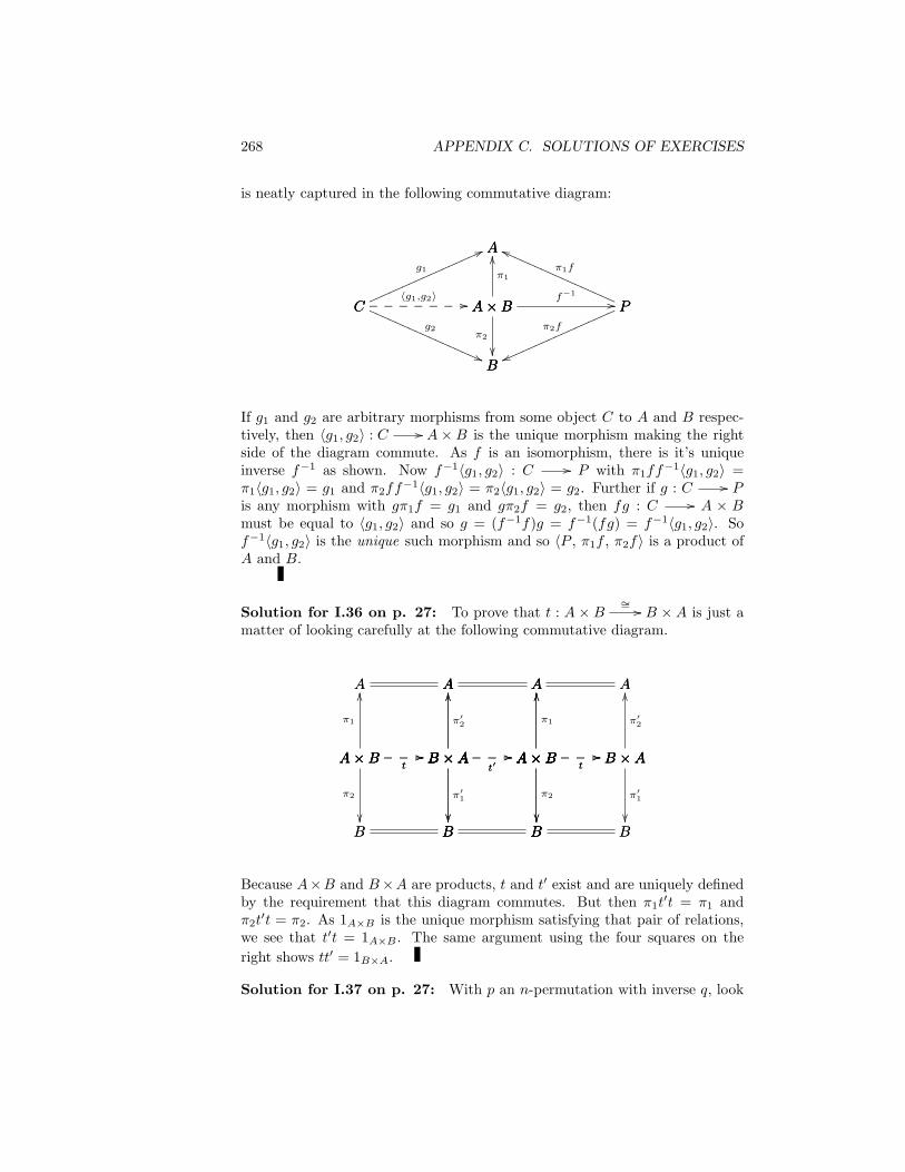
268 APPENDIX C. SOLUTIONS OF EXERCISES
is neatly captured in the following commutative diagram:
C
Ag1
66mmmmmmmmmmmmmmmmmC A×B
〈g1,g2〉 //_______C
B
g2
((QQQQQQQQQQQQQQQQQ A×B
A
π1
OO
A×B
B
π2
P
Aπ1f
hhQQQQQQQQQQQQQQQQQA×B P
f−1// P
B
π2f
vvmmmmmmmmmmmmmmmmm
If g1 and g2 are arbitrary morphisms from some object C to A and B respec-tively, then 〈g1, g2〉 : C // A×B is the unique morphism making the rightside of the diagram commute. As f is an isomorphism, there is it’s uniqueinverse f−1 as shown. Now f−1〈g1, g2〉 : C // P with π1ff
−1〈g1, g2〉 =π1〈g1, g2〉 = g1 and π2ff
−1〈g1, g2〉 = π2〈g1, g2〉 = g2. Further if g : C // Pis any morphism with gπ1f = g1 and gπ2f = g2, then fg : C // A × Bmust be equal to 〈g1, g2〉 and so g = (f−1f)g = f−1(fg) = f−1〈g1, g2〉. Sof−1〈g1, g2〉 is the unique such morphism and so 〈P , π1f , π2f〉 is a product ofA and B.
Solution for I.36 on p. 27: To prove that t : A× B∼= // B × A is just a
matter of looking carefully at the following commutative diagram.
A×B B ×At
//___
A
A×B
OO
π1
A AA
B ×A
OO
π′2
B ×A A×Bt′
//___
A
B ×A
OOA AA
A×B
OO
π1
A×B B ×At
//___
A
A×B
OOA AA
B ×A
OO
π′2
A×B B ×At
//___
B
A×B
π2
B BB
B ×A
π′1
B ×A A×Bt′
//___
B
B ×A
B BB
A×B
π2
A×B B ×At
//___
B
A×B
B BB
B ×A
π′1
Because A×B and B×A are products, t and t′ exist and are uniquely definedby the requirement that this diagram commutes. But then π1t
′t = π1 andπ2t′t = π2. As 1A×B is the unique morphism satisfying that pair of relations,
we see that t′t = 1A×B . The same argument using the four squares on theright shows tt′ = 1B×A.
Solution for I.37 on p. 27: With p an n-permutation with inverse q, look

C.1. SOLUTIONS FOR CHAPTER I 269
at the following family of commutative diagrams (with i varying from 1 to n):
Πni=1Ai Πn
i=1Ap(i)s//_____
Ai
Πni=1Ai
πi
Ai AiAi
Πni=1Ap(i)
π′q(i)
Πni=1Ap(i) Πn
i=1Ais′//_____
Ai
Πni=1Ap(i)
Ai AiAi
Πni=1Ai
πi
Πni=1Ai Πn
i=1Ap(i)s//_____
Ai
Πni=1Ai
Ai AiAi
Πni=1Ap(i)
π′q(i)
Note that s and s′ as morphisms into products are defined by the fact thatthese diagrams commute. But then s′s must be the identity on Πn
i=1Ai andss′ must be the identity on Πn
i=1Ap(i) as the identities also make the relevantdiagrams commute.
Solution for I.38 on p. 27: No! Projections need not be epimorphisms.The simplest example is ∅ × ∗ // ∗ in the category of sets. ∅ × ∗ = ∅as indeed ∅×A = ∅ for every set A, and certainly the map from the empty setto a one element set is not surjective.
Solution for I.39 on p. 28: In the category of sets, if f1 : A1// B1 and
f2 : A2// B2 are two functions, then what is (f1 × f2)(a1, a2)?
Writing (f1 × f2)(a1, a2) = (b1, b2), we have b1 = π1(f1 × f2)(a1, a2).But π1(f1, f2) = f1π1 by the definition of f1 × f2. So b1 = f1π1(a1, a2) =f1(a1). The same argument with 2 replacing 1 shows that b2 = f2(a2). So(f1 × f2)(a1, a2) = (f1(a1), f2(a2)).
Solution for I.40 on p. 28: To show that Πni=11Ai = 1ΠAi , note that, by def-
inition, Πni=11Ai is the unique morphism that fills in this family of commutative
diagrams:
Πni=1Ai Πn
i=1AiΠni=11Ai
//______
Ai
Πni=1Ai
πi
Ai Ai1Ai // Ai
Πni=1Ai
πi
But 1ΠAi fills it in equally well, ergo, they are equal.
Solution for I.41 on p. 28: With the possible exception of the equality ofthe top arc with the composition beneath it, the following family of diagrams
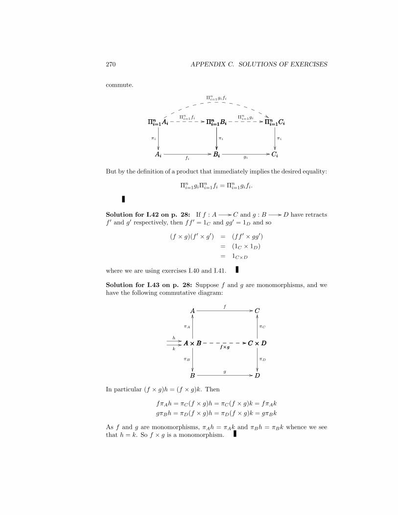
270 APPENDIX C. SOLUTIONS OF EXERCISES
commute.
Πni=1Ai Πn
i=1Ci
Πni=1gifi
&&ro
l j g d b _ \ Z W T R OL
Ai Bifi
//
Πni=1Ai
Ai
πi
Πni=1Ai Πn
i=1BiΠni=1fi //______ Πn
i=1Bi
Bi
πi
Bi Cigi
//
Πni=1Bi
Bi
Πni=1Bi Πn
i=1CiΠni=1gi //______ Πn
i=1Ci
Ci
πi
But by the definition of a product that immediately implies the desired equality:
Πni=1giΠ
ni=1fi = Πn
i=1gifi.
Solution for I.42 on p. 28: If f : A // C and g : B // D have retractsf ′ and g′ respectively, then ff ′ = 1C and gg′ = 1D and so
(f × g)(f ′ × g′) = (ff ′ × gg′)= (1C × 1D)= 1C×D
where we are using exercises I.40 and I.41.
Solution for I.43 on p. 28: Suppose f and g are monomorphisms, and wehave the following commutative diagram:
A×B C ×Df×g
//_______
A
A×B
OO
πA
A Cf // C
C ×D
OO
πC
A×Bh //
A×Bk
// A×B C ×Df×g
//_______
B
A×B
πB
B Dg // D
C ×D
πD
In particular (f × g)h = (f × g)k. Then
fπAh = πC(f × g)h = πC(f × g)k = fπAk
gπBh = πD(f × g)h = πD(f × g)k = gπBk
As f and g are monomorphisms, πAh = πAk and πBh = πBk whence we seethat h = k. So f × g is a monomorphism.

C.1. SOLUTIONS FOR CHAPTER I 271
Solution for I.44 on p. 28: If f and g have sections f ′ and g′ respectively,then f ′× g′ is a section for f × g. This follows by combining exercises I.41 andI.40. For (f × g)(f ′ × g′) = ff ′ × gf ′ = 1× 1 = 1.
Compare this with the solution to exercise I.42. The two proofs look almostthe same, although the order of composition is reversed. Notice that this is notan example of duality, because both involve products rather than interchangingproducts and sums. This proof is dual to that in the solution of exercise I.58because that is the dual theorem.
Solution for I.45 on p. 29: The method to verify that 〈f, g〉h = 〈fh, gh〉is what should by now be very familiar. 〈fh, gh〉 is the unique morphism suchthat πB〈fh, gh〉 = fh and πC〈fh, gh〉 = gh, but 〈f, g〉h has that same propertyand so they are equal.
D
B
fh
77ooooooooooooooooooooooooA
B
f
??B × C
B
πB
OO
D Ah // A B × C
〈f,g〉 //____A
C
g
?????????????? B × C
C
πC
D
C
gh
''OOOOOOOOOOOOOOOOOOOOOOOO
Solution for I.46 on p. 29: To verify that 〈f, g〉 = (f × g)∆ stare at thesetwo commutative diagrams and note that πi(f × g)∆ = f1 = f (for i = 1, 2)which is exactly the defining property of 〈f, g〉.
A×A
A
A A×A∆ //A
A
1
???????????
A
A
??
1
A
A×A
OO
A×A B ×B//
A
A×A
OO
π1
A Bf // B
B ×B
OO
π1
A Bg//
A×A
A
π2
A×A B ×Bf×g // B ×B
B
π2
B ×B
B
π2
A B ×B〈f,g〉 //A
B
g
%%KKKKKKKKKKKKKKKK
B
A
99
f
ssssssssssssssss B
B ×B
OO
π1
Solution for I.47 on p. 29: To compute ∆(x) for any x in a set X we just

272 APPENDIX C. SOLUTIONS OF EXERCISES
note that π1(∆(x)) = 1X(x) = x and π2(∆(x)) = 1X(x) = x, so ∆(x) = (x, x).
Solution for I.48 on p. 29: To compute ∆(a) for any a ∈ A with A anobject in Ab we just note that π1(∆(a)) = 1A(a) = a and π2(∆(a)) = 1A(a) =a, so ∆(a) = (a, a).
Solution for I.49 on p. 32: For any family of two or more objects,A1, · · · , An, in C prove that Σni=1Ai is isomorphic to Σn−1
i=1 Ai +An.The method is to show that Σn−1
i=1 Ai + An (with suitable morphisms) is asum of A1, · · · , An. The family of morphisms is
ι′1 = Σn−1i=1 Ai +An oo ι1 Σn−1
i=1 Aioo ι1
A1,
...
ι′j = Σn−1i=1 Ai +An oo ι1 Σn−1
i=1 Ajoo ιj
Aj ,
...
ι′n−1 = Σn−1i=1 Ai +An oo ι1 Σn−1
i=1 An−1oo ιn−1
An−1
and ι′n = Σn−1i=1 Ai +An oo ι2
An.Now given a family fi : Ai // C of morphisms we get [f1, · · · , fn−1] :
Σn−1i=1 Ai
// C. This together with fn gives us f = [[f1, · · · , fn−1], fn] as theunique morphism from Σn−1
i=1 Ai +An to C such that fι′j = fj for j = 1, · · · , n.Proposition I.2 now applies to say that Σn−1
i=1 Ai +An is canonically isomorphicto Σni=1Ai.
This is well summarized in the commutative diagram:
C
Aj
ww
fj
ooooooooooooooooooooooooooooooooooooooooooooooooooo
Σn−1i=1 Ai
Aj
ιj
C
Σn−1i=1 Ai
ss
[f1,··· ,fn−1]
gggggggggggggggggggggg Σn−1i=1 Ai +An
Σn−1i=1 Ai
ι1
C Σn−1i=1 Ai +Anoo [[f1,··· ,fn−1],fn] _____________________ Σn−1i=1 Ai +An
An
OO
ι2
C
An
kk
fn
WWWWWWWWWWWWWWWWWWWWWWWWWWWWWWWWWWWWWWWWWWWWWWW

C.1. SOLUTIONS FOR CHAPTER I 273
where j is in the range 1, · · · , n − 1 and the dotted arrows are those whoseunique existence make the diagram commute.
Compare this solution with the solution for exercise I.34 on page 26. Thetwo were written carefully to make it clear that each can be transformed intothe other by “reversing the arrows” and exchanging sums and products. Thisis an example of duality which is discussed formally in Section II.1.
Solution for I.50 on p. 32: The proof that 〈S, fι1, fι2〉 is also a sum isneatly captured in the following commutative diagram:
C
A
vv
g1
mmmmmmmmmmmmmmmmmC A+Boo [g1,g2] _______C
B
hhg2
QQQQQQQQQQQQQQQQQ A+B
A
ι1
A+B
B
OO
ι2
S
A
((
fι1
QQQQQQQQQQQQQQQQQA+B Soo f−1
S
B
66fι2
mmmmmmmmmmmmmmmmm
If g1 and g2 are arbitrary morphisms to some object C, then [g1, g2] : A+B // Cis the unique morphism making the left side of the diagram commute. As f isan isomorphism, there is it’s unique inverse f−1 as shown. Now [g1, g2]f−1 : S
// C with ι1ff−1[g1, g2] = ι1[g1, g2] = g1 and ι2ff
−1[g1, g2] = ι2[g1, g2] =g2. Further if g : S // C is any morphism with gfι1 = g1 and gfι2 = g2,then gf : A+B // must be equal to [g1, g2] and so
g = g(ff−1)= gff−1
= [g1, g2]f−1.
Thus [g1, g2]f−1 is the unique such morphism, and so 〈S, ι1f , ι2f〉 is a sum ofA and B.
Compare this solution with the solution for exercise I.35 on page 27. Thetwo were written carefully to make it clear that each can be transformed intothe other by “reversing the arrows” and exchanging sums and products. Thisis an example of duality which is discussed formally in Section II.1.
Solution for I.51 on p. 32: To prove that A+B ∼= B + A is just a matter

274 APPENDIX C. SOLUTIONS OF EXERCISES
of looking carefully at the following commutative diagram.
A+B B +Aoot
___
A
A+B
ι1
A AA
B +A
ι′2
B +A A+Boo
t′___
A
B +A
A AA
A+B
ι1
A+B B +Aoo
t___
A
A+B
A AA
B +A
ι′2
A+B B +Aoo
t___
B
A+B
ι2
OO
B BB
B +A
ι′1
OOB +A A+Boot′
___
B
B +AOO
B BB
A+B
ι2
OOA+B B +Aoot
___
B
A+BOO
B BB
B +A
ι′1
OO
Because A + B and B + A are sums, t and t′ exist and are uniquely definedby the requirement that this diagram commutes. But then tt′ι1 = ι1 andtt′ι2 = ι2. As 1A+B is the unique morphism satisfying that pair of relations,we see that tt′ = 1A+B . The same argument using the four squares on theright shows t′t = 1B+A.
Compare this solution with the solution for exercise I.36 on page 27. Thetwo were written carefully to make it clear that each can be transformed intothe other by “reversing the arrows” and exchanging sums and products. Thisis an example of duality which is discussed formally in Section II.1.
Solution for I.52 on p. 32: With p an n-permutation with inverse q, lookat the following family of commutative diagrams (with i varying from 1 to n):
Σni=1Ai Σni=1Ap(i)s//_____
Ai
Σni=1Ai
ιi
OO
Ai AiAi
Σni=1Ap(i)
ι′q(i)
OOΣni=1Ap(i) Σni=1Ais′
//_____
Ai
Σni=1Ap(i)OO
Ai AiAi
Σni=1Ai
ιi
OOΣni=1Ai Σni=1Ap(i)s
//_____
Ai
Σni=1AiOO
Ai AiAi
Σni=1Ap(i)
ι′q(i)
OO
Note that s and s′ as morphisms from sums are defined by the fact thatthese diagrams commute. But then ss′ must be the identity on Σni=1Ai ands′s must be the identity on Σni=1Ap(i) as the identities also make the relevantdiagrams commute.
Compare this solution with the solution for exercise I.37 on page 27. Thetwo were written carefully to make it clear that each can be transformed intothe other by “reversing the arrows” and exchanging sums and products. Thisis an example of duality which is discussed formally in Section II.1.
Solution for I.53 on p. 32: In a great many of the familiar categories, forexample Set, Group, Ab, Top, etc., every injection into a sum is a monomor-phism, but this is not universally true. Perhaps the simplest familiar examplewhere this is not true is CommutativeRing, the category of commutativerings. As discussed in section B.3.4 of the Catalog of Categories, the sum inthis category is the tensor product. In particular then we have the odd feature

C.1. SOLUTIONS FOR CHAPTER I 275
that the sum of two non-zero rings may be zero with the simplest examplebeing Z2 ⊗ Z3.
In any tensor product A⊗B we have
(a1 + a2)⊗ (b1 + b2) = a1 ⊗ b1 + a1 ⊗ b2 + a2 ⊗ b1 + a2 ⊗ b2.
So in Z2 ⊗ Z3 we have
1 = 1⊗ 1= (1 + 1 + 1)⊗ 1= 1⊗ 1 + 1⊗ 1 + 1⊗ 1= 1⊗ (1 + 1 + 1)= 1⊗ 0= 0
Now look at the two ring homomorphisms E0 and E1 from Z[X] to Z2 withE0(p(X)) = p(0) mod 2 and E1(p(X)) = p(1) mod 2. They are certainly notequal, but ι1E0 = ι1E1. So ι1 is not a monomorphism.
Looking ahead to dual categories (see Section II.1) we also see that theeasiest counter-example is the counter-example in exercise I.38 interpreted inthe dual category of the category of sets where the projection that is not anepimorphism in Set gives an injection that is not a monomorphism in Setop.
Solution for I.54 on p. 33: To show that Σni=11Ai = 1ΣAi , note that, bydefinition, Σni=11Ai is the unique morphism that fills in this family of commu-tative diagrams:
Σni=1Ai Σni=1AiΣni=11Ai
//______
Ai
Σni=1Ai
ιi
OO
Ai Ai1Ai // Ai
Σni=1Ai
ιi
OO
But 1ΣAi fills it in equally well, ergo, they are equal.Compare this solution with the solution for exercise I.40 on page 28. The
two were written carefully to make it clear that each can be transformed intothe other by “reversing the arrows” and exchanging sums and products. Thisis an example of duality which is discussed formally in Section II.1.
Solution for I.55 on p. 33: Consider the families of morphisms fi : Ai // Biand gi : Bi // Ci. Verify that ΣigiΣifi = Σigifi
With the possible exception of the equality of the top arc with the compo-

276 APPENDIX C. SOLUTIONS OF EXERCISES
sition beneath it, the following family of diagrams commute.
Σni=1Ai Σni=1Ci
Σni=1figi
&&ro
l j g d b _ \ Z W T R OL
Ai Bifi
//
Σni=1Ai
Ai
OO
ιi
Σni=1Ai Σni=1BiΣni=1fi //______ Σni=1Bi
Bi
OO
ιi
Bi Cigi//
Σni=1Bi
Bi
OOΣni=1Bi Σni=1Ci
Σni=1gi //______ Σni=1Ci
Ci
OO
ιi
But by the definition of a sum that immediately implies the desired equality.
Compare this solution with the solution for exercise I.41 on page 28. Thetwo were written carefully to make it clear that each can be transformed intothe other by “reversing the arrows”, including exchanging sums and products.This is an example of duality which is discussed formally in Section II.1.
Solution for I.56 on p. 33: If f : A // C and g : B // D have sectionsf ′ and g′ respectively, then ff ′ = 1A and gg′ = 1B , so (f + g)(f ′ + g′) =(ff ′ + gg′) = 1A + 1C = 1(A+B) and so f ′ + g′ is a section for f + g. Noticewe are using exercises I.54 and I.55.
Solution for I.57 on p. 33: Suppose f and g are epimorphisms, and wehave the following commutative diagram:
A+B C +Df+g
//_______
A
A+B
ιA
A Cf // C
C +D
ιC
C +D
h //C +D
k//A+B C +D
f+g//_______
B
A+B
ιB
OO
B Dg // D
C +D
ιD
OO
In particular h(f + g) = k(f + g). Then
hιCf = h(f + g)ιA = k(f + g)ιA = kιCf
hιDg = h(f + g)ιB = k(f + g)ιB = kιDg
As f and g are epimorphisms, hιC = kιC and hιD = kιD whence we see thath = k. So f + g is an epimorphism.
Compare this solution with the solution for exercise I.43 on page 28. Thetwo were written carefully to make it clear that each can be transformed into

C.1. SOLUTIONS FOR CHAPTER I 277
the other by “reversing the arrows”, exchanging sums and products and inter-changing “monomorphism” and “epimorphism”. This is an example of dualitywhich is discussed formally in Section II.1.
Solution for I.58 on p. 33: Suppose that f : A // C and g : B //
D have retracts f ′ and g′ respectively. Then f ′f = 1C and g′g = 1D, so(f ′+ g′)(f + g) = (f ′f + g′g) = 1C + 1D = 1(C +D) and so f ′+ g′ is a retractfor f + g. Notice we are using exercises I.54 and I.55.
Solution for I.59 on p. 33: In most of the familiar categories, for examplethe Set, Group, Ab, Top, etc., the sum of two monomorphisms is alwaysa monomorphism. Perhaps the simplest example where this is not true isCommutativeRing, the category of commutative rings.
As discussed in section B.3.4 of the Catalog of Categories, the sum in thiscategory is the tensor product. In particular then we have the odd featurethat the sum of two non-zero rings may be zero with one simple example beingZ2 ⊗Q.
In any tensor product A⊗B we have (a1 + a2)⊗ (b1 + b2) = a1⊗ b1 + a1⊗b2 + a2 ⊗ b1 + a2 ⊗ b2. So in Z2 ⊗Q we have
1 = 1⊗ 1= 1⊗ (1/2 + 1/2)= 1⊗ 1/2 + 1⊗ 1/2= (1 + 1)⊗ 1/2= 0⊗ 1/2= 0
Now look at 1Z2 ⊗ i with i : Z // Q the inclusion. Both of these aremonomorphisms, but Z2 ⊗ Z ∼= Z2, while Z2 ⊗ Q ∼= 0, so 1Z2 ⊗ i is not amonomorphism.
Solution for I.60 on p. 34: The method to verify that h[f, g] = [hf, hg]will be boringly familiar by now. [hf, hg] is the unique morphism such that[hf, hg]ιB = hf and [fh, gh]ιC = hg, but h[f, g] has that same property andso they are equal.
B
B + C
ιB
B
A
f
???????????B
D
hf
''OOOOOOOOOOOOOOOOOOOO
B + C A[f,g] // A D
h //
C
D
hg
77ooooooooooooooooooooC
A
g
??C
B + C
ιC
OO

278 APPENDIX C. SOLUTIONS OF EXERCISES
Again, compare this solution with the solution for exercise I.45 on page 29.The two were written carefully to make it clear that each can be transformedinto the other by “reversing the arrows”, including exchanging sums and prod-ucts. And again this is an example of duality which is discussed formally inSection II.1.
Solution for I.61 on p. 34: To verify that [f, g] = ∇(f + g) stare at thesetwo commutative diagrams and note that ∇(f + g)ιi = 1f = f (for i = 1, 2)which is exactly the defining property of [f, g].
A+A
A
OOA A+Aoo ∇A
A
__
1???????????
A
A
1
A
A+A
A+A B +Boo
A
A+A
ι1
A Boo fB
B +B
ι1
A Boog
A+A
A
OO
ι2
A+A B +Boof+gB +B
B
OO
ι2
B +B
B
OO
ι2
A B +Boo [f,g]A
B
ee
g
KKKKKKKKKKKKKKKK
B
A
f
yyssssssssssssssss B
B +B
ι1
Compare this solution with the solution for exercise I.46 on page 29. Thetwo were written carefully to make it clear that each can be transformed intothe other by “reversing the arrows”, including exchanging sums and products.And yet again this is an example of duality which is discussed formally inSection II.1.
Solution for I.62 on p. 35: From the definition, (f0 + f1)ι1(a0) = ι0f0(a0)and (f0 + f1)ι1(a1) = ι1f1(a1), i.e., (f1 + f2)(a0, 0) = (f0(a0), 0) and (f0 +f1)(a1, 1) = (f1(a1), 1). But in the category of sets A0 + A1 can be taken asA0 × 0 ∪A1 × 1
Solution for I.63 on p. 35: Verification that (A×B, ιA(a) = (a, 0), ιB(b) =(0, b)) is indeed a sum of A and B in Ab has several easy parts. The firstis the trivial observation that ιA and ιB are actually group homomorphisms.The next is to check that for any two homomorphisms f : A // C andg : B // C, [f, g] defined by [f, g](a, b) = f(a) + g(b) is indeed a group

C.1. SOLUTIONS FOR CHAPTER I 279
homomorphism:
[f, g]((a1, b1) + (a2, b2)) = [f, g](a1 + a2, b1 + b2)= f(a1 + a2) + g(b1 + b2)= f(a1) + f(a2) + g(b1) + g(b2)= f(a1) + g(b1) + f(a2) + g(b2)= [f, g](a1, b1) + [f, g](a2, b2)
and [f, g](0, 0) = f(0) + g(0) = 0 + 0 = 0.Finally we must check that if h : A × B // C is any other group homo-
morphism such that hιA = f and hιB = g, then h = [f, g]:
h(a, b) = h((a, 0) + (0, b))= h(a, 0) + h(0, b)= hιA(a) + hιB(b)= f(a) + g(b)= [f.g](a, b)
Solution for I.64 on p. 35: To compute ∇(a1, a2) for any (a1, a2) ∈ A⊕Awith A any object in Ab, note that (a1, a2) = (a1, 0) + (0, a2) = ι1(a1) + ι2(a2)and so ∇(a1, a2) = ∇(ι1(a1) + ι2(a2)) = ∇(ι1(a1)) + ∇(ι2(a2)) = 1A(a1) +1A(a2) = a1 + a2.
Solution for I.65 on p. 35: From the definition, (f1 + f2)ι1(a1) = ι1f1(a1)and (f1 + f2)ι2(a2) = ι2f2(a2), i.e., (f1 + f2)(a1, 0) = (f1(a1), 0) and (f1 +f2)(0, a2) = (0, f2(a2)). And as (a1, a2) = (a1, 0) + (0, a2) and f1 + f2 is ahomomorphism we have (f1 + f2)(a1, a2) = (f1(a1), f2(a2)).
Solution for I.66 on p. 35: Verification that (A × B, ιA(a) = (a, 0),ιB(b) = (0, b)) is indeed a sum of A and B in Vect has several easy parts. Thefirst is the trivial observation that ιA and ιB are actually linear transformations.The next is to check that for any two linear transformations f : A // C andg : B // C, [f, g] defined by [f, g](a, b) = f(a) + g(b) is indeed a lineartransformation:
[f, g]((a1, b1) + (a2, b2)) = [f, g](a1 + a2, b1 + b2)= f(a1 + a2) + g(b1 + b2)= f(a1) + f(a2) + g(b1) + g(b2)= f(a1) + g(b1) + f(a2) + g(b2)= [f, g](a1, b1) + [f, g](a2, b2)

280 APPENDIX C. SOLUTIONS OF EXERCISES
[f, g](λ(a, b)) = [f, g](λa, λb)= f(λa) + f(λb)= λf(a) + λg(b)= λ(f(a) + g(b))= λ[f, g](a, b)
and [f, g](0, 0) = f(0) + g(0) = 0 + 0 = 0.Finally we must check that if h : A × B // C is any other linear trans-
formation such that hιA = f and hιB = g, then h = [f, g]:
h(a, b) = h((a, 0) + (0, b))= h(a, 0) + h(0, b)= hιA(a) + hιB(b)= f(a) + g(b)= [f.g](a, b)
Solution for I.67 on p. 35: To compute ∇(a1, a2) for any (a1, a2) ∈ A⊕Awith A any vector space in Vect, note that (a1, a2) = (a1, 0) + (0, a2) =ι1(a1)+ι2(a2) and so ∇(a1, a2) = ∇(ι1(a1)+ι2(a2)) = ∇(ι1(a1))+∇(ι2(a2)) =1A(a1) + 1A(a2) = a1 + a2.
Solution for I.68 on p. 35: From the definition, (f1 + f2)ι1(a1) = ι1f1(a1)and (f1 + f2)ι2(a2) = ι2f2(a2), i.e., (f1 + f2)(a1, 0) = (f1(a1), 0) and (f1 +f2)(0, a2) = (0, f2(a2)). And as (a1, a2) = (a1, 0) + (0, a2) and f1 + f2 is alinear transformation we have (f1 + f2)(a1, a2) = (f1(a1), f2(a2)).
Solution for I.69 on p. 36: Prove that any two final objects in C areisomorphism, and the isomorphism is unique.
If F and F’ are both final objects, then there are unique morphisms F! // F ′ and F ′
F //. But then the composition F! // F ′
! // F must bethe unique morphism from F // F , which is 1F . Equally well the compositionin the other order must be 1F ′ .
Solution for I.70 on p. 36: There is hardly anything to say. For eachand every object C, not just 1, there is a bijection between pairs of morphisms(f : C // A, g : C // B) and morphisms 〈f, g〉 : C // A × B of C toA × B – that is just a slightly different way of stating the definition of theproduct.
Solution for I.71 on p. 36: Here is the diagram that exhibits (A, 1A, !) as

C.1. SOLUTIONS FOR CHAPTER I 281
a product of A and 1:
A
1
!
C Af___ //___C
1
!
??????????????
A
C
??
f
A
A
OO
1A
Solution for I.72 on p. 36: To verify that every point p : 1 // C is amonomorphism, consider the diagram
Bg1 //g2
// 1p // C
By the definition of a final object any two morphisms g1, g2 : C // 1 areequal, so certainly pg1 = pg2 ⇒ g1 = g2.
Solution for I.73 on p. 37: If 0 and 0’ are both initial objects, then thereare unique morphisms 0 // 0′ and 0′ // 0. But then the composition 0
// 0′ // 0 must be the unique morphism from 0 // 0, i.e., 10. Equallywell the composition in the other order must be 10′ .
Compare this solution with the solution for exercise I.69 on page 37. Thetwo were written carefully to make it clear that each can be transformed into theother by “reversing the arrows”, including exchanging initial and final objects.In this particular case the proofs look identical, but this is yet another exampleof duality which is discussed formally in Section II.1.
Solution for I.74 on p. 37: Here is the diagram that exhibits (A, 1A, !) asa sum of A and 0:
A
0
OO
!
C Aoo f___ ___C
0
__
!
??????????????
A
C
f
A
A
1A

282 APPENDIX C. SOLUTIONS OF EXERCISES
Compare this solution with the solution for exercise I.71 on page 36. Thetwo were written carefully to make it clear that each can be transformed intothe other by “reversing the arrows”, including exchanging sums and productsand initial and final objects. Again this is yet another example of duality whichis discussed formally in Section II.1.
Solution for I.75 on p. 40: Verifying that the morphisms Σni=1Ai// Πmj=1Bj
are exactly the “matrices”
M =
f11 f12 · · · f1m
f21 f22 · · · f2m
. . .fn1 fn2 · · · fnm
where πjMιi = fij is entirely a matter of unwinding the definitions. Givenf : Σni=1Ai
// Πmj=1Bj we certainly get the matrix M = (fij) with fij =
πjfιi.In the reverse direction if we are given an n × m-matrix (fij) of mor-
phisms fij : Ai // Bj , then for each fixed i we get the unique morphism〈fi1, · · · , fim〉 : Ai // Πm
j=1Bj whose composition with πj is fij . And fromall of those we get the unique morphism f (shown in “matrix” form in thefollowing diagram) whose composition with ιi is 〈fi1, · · · , fim〉.
Πmj=1Bj Bjπj
//
Σni=1Ai
Πmj=1Bj
0BBBBBB@〈f11, f12, · · · , f1m〉〈f21, f22, · · · , f2m〉
. . .〈fn1, fn2, · · · , fnm〉
1CCCCCCA
Σni=1Ai Aioo ιiAi
Bj
fij
Ai
Πmj=1Bj
〈fi1,··· ,fim〉
yyss
ss
ss
ss
ss
ss
Equally well, the n×m-matrix (fij) of morphisms fij : Ai // Bj , then foreach fixed j we get the unique morphism [f1j , · · · , fnj ] : Σni=1Ai
// Bj whosecomposition with ιi is fij . And from all of those we get the unique morphism f(shown in “matrix” form in the following diagram) whose composition with πjis [f1j , · · · , fnj ]. Notice as a result that the two morphisms from ΣAi // ΠBjdefined here and above are equal.

C.1. SOLUTIONS FOR CHAPTER I 283
Πmj=1Bj Bjπj
//
Σni=1Ai
Πmj=1Bj
⟨0BBBBBB@f11,f12
...fn1
1CCCCCCA,0BBBBBB@f12,f22
...fn2
1CCCCCCA,··· ,0BBBBBB@f1m,f2m
...fnm
1CCCCCCA⟩
Σni=1Ai Aioo ιiAi
Bj
fij
Σni=1Ai
Bj
[f1j ,··· ,fnj ]
%%KK
KK
KK
KK
KK
KK
Solution for I.76 on p. 41: In order to show that I : X + Y // X × Ycorresponds exactly to the inclusion (X×y0∪x0×Y ) ⊂ X×Y we recall theconstruction of the sum of two pointed sets (see I.45): 〈X,x0〉+ 〈Y, y0〉 = 〈X×y0∪x0×Y, 〈x0, Y0〉〉, ιX : 〈X,x0〉 // 〈X,x0〉+ 〈Y, y0〉 by ιX(x) = 〈x, y0〉and ιY : 〈Y, y0〉 // 〈X,x0〉+ 〈Y, y0〉 by ιX(y) = 〈x0, y〉
And what is I?
I(t) =
〈t, y0〉 if t ∈ X〈x0, t〉 if t ∈ Y
which is exactly the desired inclusion.Now if X and Y are not singletons, then there is x1 ∈ X with x1 6= x0 and
y1 ∈ Y with y1 6= y0. But then (x1, y1) ∈ X × Y , but it is not in the image ofI.
Solution for I.77 on p. 43: Starting with f : A // C and g : B // Dwe compute the the matrix f+g by starting with the fact that (f+g)ιA = ιCfand (f + g)ιB = ιDg. We need πC(f + g)ιA, πC(f + g)ιB , πD(f + g)ιA, andπD(f + g)ιB . But πC(f + g)ιA = πCιCf = 1Cf = f and πC(f + g)ιB =πCιDf = 0f = 0. A similar computation for the other two shows that thematrix is (
f 00 g
)And this is what we previously computed as the matrix of f × g
Solution for I.78 on p. 43: To verify that the matrices of Πni=1fi :
⊕ni=1Ai
// ⊕ni=1Bi
and Σni=1fi :⊕n
i=1Ai// ⊕n
i=1Bi isf1 0 · · · 00 f2 · · · 0
. . .0 0 · · · fn
is one of those cases where the use of indices makes the computation a littleeasier. The ij-entry of the matrix for the product is πi(Πn
k=1fk)ιj which is, bydefinition, equal to fiπkιj which is fi when i = j and 0 otherwise.

284 APPENDIX C. SOLUTIONS OF EXERCISES
Equally well the ij-entry of the matrix for the sum is πi(Σnk=1fk)ιj whichis, by definition, equal to πiιjfj which is fi when i = j and 0 otherwise.
Solution for I.79 on p. 44: In the category of Abelian groups, ∆ : A // A×Ais ∆(a) = (a, a), so (f M g)(a) = [f, g](a, a) = f(a) + g(a). (Recall exer-cise I.63.) And (fOg)(a) = ∇(f(a), g(a)) = f(a) + g(a).
Solution for I.80 on p. 45: To show that f = 0+f we will use the followingcommutative diagram:
A 0! // 0
B
!
???????????
A
A
1
??A⊕A
A
πA
OO 0
0⊕A
ι0
A A⊕A∆ // A⊕A 0⊕A
!⊕1 // 0⊕A B[!,f //]A
A
1
??????????? A⊕A
A
πA
A
0⊕A
ιA
OO
A A1 // A
B
f
??
Notice that the left two triangle are just exhibiting A ⊕ A as a product,
and showing the definition of ∆. The sequence A ! // 0 ! // B is factoring0 : A // B. The middle squares exhibit the definition of !⊕1A, and the righttriangle on the right exhibit the definition of [!, f ]. Recall from exercise I.74that here ιA : A // 0⊕A is an isomorphism.
Now the application of this diagram here is first that [!, f ](! ⊕ 1A)∆ =f1A1A = f , and second that [!, f ](! ⊕ 1A)∆ = [0, f ]∆ = 0 + f . So f = 0 + f .
Now to get f + 0 = f just interchange the top and bottom of the diagram.
Solution for I.81 on p. 45: For h(f + g) we have:
h(f + g) = h(f M g) by Proposition I.4= h[f, g]∆ by definition I.49= [hf, hg]∆ by exercise I.60= hf M hg by definition I.49= hf + hg by Proposition I.4
And for (f + g)e we have:
(f + g)e = (fOg)e by Proposition I.4= ∇〈f, g〉e by definition I.50= ∇〈fe, ge〉 by exercise I.45= feOge by definition I.50= fe+ ge by Proposition I.4

C.1. SOLUTIONS FOR CHAPTER I 285
Solution for I.82 on p. 45: In order to verify that ιAπA+ιBπB = 1A⊕B let’slook at the matrix of ιAπA + ιBπB . For that we look at the four components:
πA(ιAπA + ιBπB)ιA = πAιAπAιA + πAιBπBιA
= 1A1A + 00= 1A + 0= 1A
πA(ιAπA + ιBπB)ιB = πAιAπAιB + πAιBπBιB
= 1A0 + 01B= 0 + 0= 0
πB(ιAπA + ιBπB)ιA = πBιAπAιA + πBιBπBιA
= 01A + 1B0= 0 + 0= 0
πB(ιAπA + ιBπB)ιB = πBιAπAιB + πBιBπBιB
= 00 + 1B1B= 0 + 1B= 1B
So the matrix of ιAπA + ιBπB is the identity matrix. But only the identitymorphism has that matrix!
Solution for I.83 on p. 48: To show that there is a category, MagmaC ,with objects the magmas in C and as morphisms the magma morphisms, wehave to specify the identity morphisms, the composition and verify the requiredidentities. Of course the identity morphism for a magma (M,µ) will just be theidentity morphism on the object M which is clearly a magma morphism. Andcomposition of magma morphisms will just be composition of the morphismsin C . That composition of two magma morphisms is again a magma morphism

286 APPENDIX C. SOLUTIONS OF EXERCISES
is clear from
N ×N Nµ//
M ×M
N ×N
f×f
M ×M Mµ // M
N
f
P × P Pµ//
N ×N
P × P
g×g
N ×N Nµ // N
P
g
and the fact (cf. exercise I.41) that (g × g)(f × f) = (gf × gf). Finallyassociativity of composition of magma morphisms and the identities for identitymorphisms follows from associativity of composition of morphisms in C .
Solution for I.84 on p. 49:If C is any category with finite products, then MagmaC is also category
with finite products. As noted in the text, when M1, . . . , Mn are magmas inC (with binary operations µ1, . . . , µn), we define a binary operation, µ, onΠn
1Mi as the composite:
Πn1Mi ×Πn
1Mi
∼= // Πn1 (Mi ×Mi)
Πn1 µi // Πn1Mi
where the isomorphism is a special case of the result in exercise I.37.To verify this is a product in MagmaC we need to confirm that the pro-
jection morphisms πi : Πni=1Mi
// Mi are magma morphisms, and that forevery family of magma morphisms fi : M // Mi, the unique morphismf = 〈f1, · · · , fn〉 : M // Πn
i=1Mi making the product diagram commute(which exists because we have the product in C ) is actually a magma mor-phism.
That each projection πi is a magma homomorphism is seen by inspectingthe following diagram:
Πnj=1(Mj ×Mj) Mi ×Mi
//
Πnj=1Mj ×Πn
j=1Mj
Πnj=1(Mj ×Mj)
∼=
Πnj=1Mj ×Πn
j=1Mj
Mi ×Mi
πi×πi
''OOOOOOOOOOOOOOO
Πnj=1Mj Miπi
//
Πnj=1(Mj ×Mj)
Πnj=1Mj
Πµj
Πnj=1(Mj ×Mj) Mi ×Mi
πi // Mi ×Mi
Mi
µi
The top triangle is commutative because the isomorphism is exactly the uniquemorphism that makes it commute. While the bottom square is commutativebecause this is exactly the definition of Πµj .

C.1. SOLUTIONS FOR CHAPTER I 287
To see that f =< f1, · · · , fn > is a magma morphism we need to show thefollowing diagram commutes:
M ×M Πnj=1Mj ×Πn
j=1Mj
f×f //M ×M
Πnj=1(Mj ×Mj)
M ×M
Πnj=1(Mj ×Mj)
Πnj=1Mj ×Πn
j=1Mj
Πnj=1(Mj ×Mj)
∼=
M ×M
M
µ
Πnj=1(Mj ×Mj)
Πnj=1Mj
Πµj
M Πn
j=1Mj
f //MM Πnj=1MjΠnj=1Mj
To show that two morphisms into the product Πnj=1Mj are equal we need
to show their compositions with the projections into each factor are equal. Tosee that let’s add a few more morphisms:
M ×M Πnj=1Mj ×Πn
j=1Mj
f×f //M ×M
Πnj=1(Mj ×Mj)
F
**TTTTTTTTTTTTTTTTTTTTTTT Πnj=1Mj ×Πn
j=1Mj
Πnj=1(Mj ×Mj)
∼=
M ×M
M
µ
Πnj=1(Mj ×Mj)
Πnj=1Mj
Πµj
M Πn
j=1Mj
f //M
Mi
fi
**TTTTTTTTTTTTTTTTTTTTTTTTTTTT Πnj=1Mj
Mi
πi
(where we’ve written F for 〈f1 × f1, · · · , fn × fn〉 to make the diagram lesscluttered.) The top triangle commutes by the definition of the isomorphism,while the bottom triangle commutes by the definition of f . So we are left toverify that πi(Πµj)F = fiµ. But πi(Πµj)F = µiπiF by definition of Πµj , andthis in turn is equal to µi(fi × fi) by definition of F . And finally this is equalto fiµ because fi is a magma morphism by hypothesis.
Solution for I.85 on p. 49: As with most everything here, verification thatfor M and N magmas and h : M // N a magma morphism, then Hom(C, h)is a magma homomorphism is just a matter of unwinding the definitions. And

288 APPENDIX C. SOLUTIONS OF EXERCISES
as usual a commutative diagram helps:
C M ×M〈f,g〉 //C
N ×N
〈hf,hg〉??????????? M ×M
N ×N
N ×N Nµ//
M ×M
N ×N
h×h
M ×M Mµ // M
N
h
Hom(C, h)(f M g) = h(f M g)= hµ〈f, g〉= 〈f, g〉(h× h)µ= 〈hf, hg〉µ= hf M hg
= Hom(C, h)(f) M Hom(C, h)(g)
Solution for I.86 on p. 49: Verifying that for any magma M and h anymorphism at all Hom(h,M) is a magma homomorphism is even simpler thanthe last exercise:
Hom(h,M)(f M g) = (f M g)h= µ〈f, g〉h= µ〈fh, gh〉= fh M gh
= Hom(h,M)(f) M Hom(h,M)(g)
Solution for I.87 on p. 51: To show that there is a category, ComagmaC ,with objects the comagmas in C and as morphisms the comagma morphisms,we have to specify the identity morphisms, the composition and verify therequired identities. Of course the identity morphism for a comagma (C, ν) willjust be the identity morphism on the object C which is clearly a comagmamorphism. And composition of comagma morphisms will just be compositionof the morphisms in C . That composition of two comagma morphisms is again

C.1. SOLUTIONS FOR CHAPTER I 289
a comagma morphism is clear from
D +D Dooν
C + C
D +D
OO
f+f
C + C Coo νC
D
OO
f
E + E Eooν
D +D
E + E
OO
g+g
D +D Doo D
E
OO
g
and the fact (cf. exercise I.55) that (f + f)(g + g) = (fg + fg). Finally asso-ciativity of composition of comagma morphisms and the identities for identitymorphisms follows from associativity of composition of morphisms in C .
Solution for I.88 on p. 51: To verify that h : D // C a comagmamorphism, implies Hom(h,X) is a magma homomorphism is just a matter ofunwinding the definitions. And as usual a commutative diagram helps:
X C + Coo [f,g]X
D +D
__
[hf,hg]??????????? C + C
D +D
OO
D +D Dooν
C + C
D +D
OO
h+h
C + C Coo νC
D
OO
h
Hom(h,X)(fOg) = (fOg)h= [f, g]νh= ν(h+ h)[f, g]= ν[hf, hg]= hfOhg
= Hom(h,X)(f)OHom(h,X)(g)
Compare this solution with that of I.85. This is yet another example ofduality, though now “reversing arrows” results not only in interchanging sumsand products, but also interchanging magmas and comagmas.
Solution for I.89 on p. 51: Verifying that for any comagma C and h anymorphism at all Hom(C, h) is a magma homomorphism is even simpler than

290 APPENDIX C. SOLUTIONS OF EXERCISES
the last exercise:
Hom(C, h)(fOg) = h(fOg)= h[f, g]ν= [hf, hg]ν= hfOhg
= Hom(C, h)(f)OHom(C, h)(g)
Compare this solution with that of exercise I.86. This is yet another exam-ple of duality, though now “reversing arrows” results not only in interchangingsums and products, but also interchanging magmas and comagmas.
Solution for I.90 on p. 52: The exercise here is to show that if C is anycategory with finite sums, then ComagmaC is also category with finite sums.
As noted in the text, when C1, . . . , Cn are comagmas in C (with co-operations ν1, . . . , νn), we can define a co-operation, ν, on Σn1Ci as the com-posite:
Σn1CiΣn1 νi // Σn1 (Ci + Ci)
∼= // Σn1Ci + Σn1Ci
where the isomorphism is a special case of the result in exercise I.52.To verify this is a sum in ComagmaC we need to confirm that the injection
morphisms ιi : Ci // Σni=1Ci are comagma morphisms, and that for everyfamily of comagma morphisms fi : C // Ci, the unique morphism f =[f1, · · · , fn] : C // Σni=1Ci making the sum diagram commute (which existsbecause we have the sum in C ) is actually a comagma morphism.
That each injection ιi is a comagma homomorphism is seen by inspectingthe following diagram:
Σnj=1(Cj + Cj) Ci + Cioo
Σnj=1Cj + Σnj=1Cj
Σnj=1(Cj + Cj)
OO
∼=
Σnj=1Cj + Σnj=1Cj
Ci + Ci
ggιi+ιi
OOOOOOOOOOOOOOO
Σnj=1Cj Ciooιi
Σnj=1(Cj + Cj)
Σnj=1Cj
OO
Σνj
Σnj=1(Cj + Cj) Ci + Cioo ιiCi + Ci
Ci
OO
νi
The top triangle is commutative because the isomorphism is exactly the uniquemorphism that makes it commute. While the bottom square is commutativebecause this is exactly the definition of Σνj .
To see that f = [f1, · · · , fn] is a comagma morphism we need to show the

C.1. SOLUTIONS FOR CHAPTER I 291
following diagram commutes:
C + C Σnj=1Cj + Σnj=1Cjoo f+f
C + C
Σnj=1(Cj + Cj)
C + C
Σnj=1(Cj + Cj)
Σnj=1Cj + Σnj=1Cj
Σnj=1(Cj + Cj)
OO
∼=
C + C
C
OO
ν Σnj=1(Cj + Cj)
Σnj=1Cj
OO
Σνj
C Σnj=1Cjoo f
CC Σnj=1CjΣnj=1Cj
To show that two morphisms from the sum Σnj=1Cj are equal we need toshow their compositions with the injections from each summand are equal. Tosee that let’s add a few more morphisms:
C + C Σnj=1Cj + Σnj=1Cjoo f+f
C + C
Σnj=1(Cj + Cj)
jj
F
TTTTTTTTTTTTTTTTTTTTTTTT Σnj=1Cj + Σnj=1Cj
Σnj=1(Cj + Cj)
OO
∼=
C + C
C
OO
ν Σnj=1(Cj + Cj)
Σnj=1Cj
OO
Σνj
C Σnj=1Cjoo f
C
Ci
jj
fi
TTTTTTTTTTTTTTTTTTTTTTTTTTTTT Σnj=1Cj
Ci
OO
ιi
(where we’ve written F for [f1 + f1, · · · , fn + fn] to make the diagram lesscluttered.) The top triangle commutes by the definition of the isomorphism,while the bottom triangle commutes by the definition of f . So we are left toverify that F (Σνj)ιi = νfi.
But F (Σνj)ιi = Fιiνi by definition of Σνj , and this in turn is equal to(fi + fi)νi by definition of F . And finally this is equal to νfi because fi is acomagma morphism by hypothesis.
Compare this solution with that of exercise I.84. This is yet another exam-ple of dual proofs of dual theorems. In particular this solution was carefullyproduced by taking the solution of exercise I.84 and making exactly the changesnecessary to produce the dual proof.

292 APPENDIX C. SOLUTIONS OF EXERCISES
Solution for I.91 on p. 56: The proof of parts (4.) – (6.) of Proposition I.8were left as an exercise because they are dual to parts (1.) – (3.). Here are thedual proofs:
For (4.) note that [ι1, 0] M= ι1 + 0 = ι1 and [0, ι2] M= 0 + ι2 = ι2 as 0 isthe identity for +, the induced binary operation on Hom(A, •)
For (5.) we see that [M, 1] M=M +1, while [1,M] M= 1+ M. But we knowthat + is commutative, so M +1 = 1+ M.
For (6.) we observe that M t is also a binary operation on A for which 0is the identity in the monoid Hom(A, •). But such a binary operation on A isunique, so M t =M.
Solution for I.92 on p. 58: To show that there is a category, MonoidC ,with objects the monoids in C and as morphisms the monoid morphisms, wehave to specify the identity morphisms, the composition and verify the requiredidentities. Of course the identity morphism for a monoid (M,µ) will just be theidentity morphism on the object M which is clearly a monoid morphism. Andcomposition of monoid morphisms will just be composition of the morphismsin C . The only work to be done is verification that composition of two monoidmorphisms is again a monoid morphism. The first part of that was done inverifying the existence of MagmaC in the solution to exercise I.83. For thesecond part suppose f : M // N and g : N // P are monoid morphisms,so in particular fζM = ζN and gζN = ζP , then gfζM = ζP and so gf is amonoid morphism as well.
That identity morphisms behave as required and that composition is asso-ciative is true in MonoidC just because it is true in C .
Solution for I.93 on p. 58: In exercise I.92 you displayed the category ofmonoids in C , MonoidC . For the category of commutative monoids in C thereis really nothing more to say – the identities, law of composition and variousidentities all come from those same items in MonoidC . Indeed this is just oneof many examples of a full subcategory defined by a class of objects in somecategory (see section I.1.2, especially definition I.12.)
Solution for I.94 on p. 59: If C is any category with finite products,then MonoidC is also a category with finite products. Much of the work ofproving this has already been done in exercise I.84. What remains to be done is(1.) check that when M1, . . . , Mn are monoids, the product binary operationon the magma Πn
i=1Mi also satisfies the associative law (see definition I.59);(2.) define an identity ζ : 1 // Πn
i=1Mi (including verifying the identitylaw holds); (3.) verify that each of the projection morphisms πi : Πn
i=1Mi// Mi preserves the identity; and (4.) show that for every family of monoid
morphisms fi : M // Mi, the unique magma morphism f = 〈f1, · · · , fn〉 : M// Πni=1Mi making the product diagram commute respect the identity.
(1.) Taking M = Πni=1Mi the associative law asserts the following diagram

C.1. SOLUTIONS FOR CHAPTER I 293
is commutative:
M ×M Mµ//
M ×M ×M
M ×M
〈µ,1〉
M ×M ×M M ×M〈1,µ〉 // M ×M
M
µ
As always, to verify that two morphisms into a product are equal it isenough to verify that their composites with all of the projection morphismsare equal. So we will verify that the following diagrams are commutative:
Mi ×Mi ×Mi Mi ×Mi1×µi//
M ×M ×M
Mi ×Mi ×Mi
πi×πi×πi
M ×M ×M M ×M1×µ // M ×M
Mi ×Mi
πi×πi
Mi ×Mi Miµi
//
M ×M
Mi ×Mi
πi×πi
M ×M Mµ // M
Mi
πi
Mi ×Mi ×Mi Mi ×Miµi×1//
M ×M ×M
Mi ×Mi ×Mi
πi×πi×πi
M ×M ×M M ×Mµ×1 // M ×M
Mi ×Mi
πi×πi
Mi ×Mi Miµi
//
M ×M
Mi ×Mi
πi×πi
M ×M Mµ // M
Mi
πi
Notice that the only differences in the diagrams are the 1 × µ and 1 × µiin the top diagram versus µ× 1 and µi × 1 in the bottom. But we know thatfor all i the bottom rows of the two diagrams are equal because the binaryoperations µi are associative. So if the diagrams are commutative, it followsthat the top rows are equal and so µ is also associative.
In the top diagram, the right hand square is commutative by the definitionof µ = Πn
i=1µi. For the left hand square note that (πi×πi)(1×µ) = πi×(πiµ) =πi × (µi(πi × πi)) = (1× µi)(πi × πi × πi)
The lower diagram is commutative by essentially the same argument.(2.) With the identity on M defined as ζ = 〈ζ1, · · · , ζn〉 : 1 // Πn
i=1Mi,we want to verify that the following two triangles commute.
M × 1 M ×M1M×ζ //M × 1
M
π1
$$JJJJJJJJJJJJJJ M ×M
M
µ
M ×M 1×Moo ζ×1MM ×M
M
1×M
M
π2
zztttttttttttttt
Again it is enough to verify that their composites with all of the projec-tion morphisms are equal. So we first note that the following diagrams arecommutative:

294 APPENDIX C. SOLUTIONS OF EXERCISES
Mi × 1 Mi ×Mi1×ζi//
M × 1
Mi × 1
πi×1
M × 1 M ×M1×ζ // M ×M
Mi ×Mi
πi×πi
Mi ×Mi Miµi
//
M ×M
Mi ×Mi
πi×πi
M ×M Mµ // M
Mi
πi
Mi × 1 Mi ×Miζi×1//
M × 1
Mi × 1
πi×1
M × 1 M ×Mζ×1 // M ×M
Mi ×Mi
πi×πi
Mi ×Mi Miµi
//
M ×M
Mi ×Mi
πi×πi
M ×M Mµ // M
Mi
πi
and observe that the bottom row in both cases is π1 : Mi × 1 // Mi becauseζi is the identity for µi. But that says for every i, πiµ(1×ζ) = π1(πi×1) whichin turn is equal to πiπ1 and so µ(1× ζ) = π1.
(3.) To verify that each of the projection morphisms πi : Πni=1Mi
// Mi
preserves the identity is just to note the definition of ζ: πiζ = ζi.(4.) And finally verifying that f = 〈f1, · · · , fn〉 always respects the identity
is just noting fζ = 〈f1ζ1, · · · , fnζn〉 = 〈ζ1, · · · , ζn〉 = ζ.
Solution for I.95 on p. 59: Suppose h : M // N is a monoid mor-phism in C and C is any object, then in exercise I.85 you showed that h∗ fromHom(C,M) to Hom(C,N) is a magma morphism. It is a monoid homomor-phism because hζ = ζ implies that h∗ζ∗ = ζ∗, i.e., h∗(ζ) = ζ where these lastζ’s are the identities in Hom(C,M) and Hom(C,N).
Solution for I.96 on p. 59: Considering h : D // C and the inducedfunction h∗ : Hom(C,M) // Hom(D,M) for a monoid M in C , half thework to show h∗ is a monoid homomorphism was done in exercise I.86. Whatremains is to see that h∗(ζ) = ζ and that is just because !h =! where the !’sare the unique morphisms to the final object.
Solution for I.97 on p. 61: Most of the work to prove Theorem I.5 was donein proving Theorem I.4. From that we have the unique morphisms so that (M ,µ, ζ) is a monoid inducing the given monoid structure in Hom(C,M). All thatremains is to prove the binary operation commutative. which means that thediagram
M ×M
M
µ
???????????M ×M M ×Mt // M ×M
M
µ

C.1. SOLUTIONS FOR CHAPTER I 295
is commutative. Recall that µ = π1Oπ2 and t = 〈π2, π1〉 so µt = π2Oπ1. Byhypothesis O is commutative, so π1Oπ2 = π2Oπ1 and µt = µ.
Solution for I.98 on p. 62: To show that there is a category, ComonoidC ,with objects the comonoids in C and as morphisms the comonoid morphisms,we have to specify the identity morphisms, the composition and verify the re-quired identities. Of course the identity morphism for a comonoid (C, ν) willjust be the identity morphism on the object C which is clearly a comonoidmorphism. And composition of comonoid morphisms will just be compositionof the morphisms in C . The only work to be done is verification that compo-sition of two comonoid morphisms is again a comonoid morphism. The firstpart of that was done in verifying the existence of ComagmaC in the solutionto exercise I.87. For the second part suppose f : C // D and g : D // Eare comonoid morphisms, so in particular ηCf = ηD and ηDg = ηE , thenηCgf = ηE and so gf is a comonoid morphism as well.
That identity morphisms behave as required and that composition is asso-ciative is true in ComonoidC just because it is true in C .
Compare this solution to the solution of exercise I.92. This is still anotherexample of dual proofs of dual theorems. In particular this solution was care-fully produced by taking the solution of exercise I.92 and making exactly thechanges necessary to produce the dual proof.
Solution for I.99 on p. 62: In exercise I.98 you displayed the category ofcomonoids in C , ComonoidC . For the category of co-commutative comonoidsin C there is really nothing more to say – the identities, law of compositionand various identities all come from those same items in ComonoidC . Indeedthis is just one of many examples of a full subcategory defined by a class ofobjects in some category (see section I.1.2, especially definition I.12.)
Compare this solution to the solution of exercise I.93. This time the twoproofs are nearly identical, but this is still an example of dual proofs of dualtheorems. In particular this solution was produced by taking the solutionof exercise I.92 and following using the meaning of “dual” to make exactlythe changes necessary to produce the dual proof, which in this case was justchanging a few words and symbols.
Solution for I.100 on p. 63: If C is any category with finite sums, thenComonoidC is also a category with finite sums. Much of the work of provingthis has already been done in exercise I.90. What remains to be done is (1.)check that when C1, . . . , Cn are monoids, the co-operation on the magmaΣni=1Ci also satisfies the associative law (see definition I.62); (2.) define anco-unit η : Σni=1Ci
// 1 (including verifying the co-unit law holds); (3.)verify that each of the inclusion morphisms ιi : Ci // Σni=1Ci preserves theco-unit; and (4.) show that for every family of comonoid morphisms fi : Ci
// C, the unique co-magma morphism f = [f1, · · · , fn] : Σni=1Ci// C
making the sum diagram commute respect the identity.

296 APPENDIX C. SOLUTIONS OF EXERCISES
1. Taking C = Σni=1Ci the co-associative law asserts the following diagramis commutative:
C + C Cooν
C + C + C
C + C
OO
[ν,1]
C + C + C C + Coo [1,ν]C + C
C
OO
ν
As always, to verify that two morphisms from a sum are equal it is enoughto verify that their composites with all of the inclusion morphisms areequal. So we will verify that the following diagrams are commutative:
Ci + Ci + Ci Ci + Cioo1+νi
C + C + C
Ci + Ci + Ci
OO
ιi+ιi+ιi
C + C + C C + Coo 1+νC + C
Ci + Ci
OO
ιi+ιi
Ci + Ci Ciooνi
C + C
Ci + Ci
OO
ιi+ιi
C + C Coo νC
Ci
OO
ιi
Ci + Ci + Ci Ci + Ciooνi+1
C + C + C
Ci + Ci + Ci
OO
ιi+ιi+ιi
C + C + C C + Coo ν+1C + C
Ci + Ci
OO
ιi+ιi
Ci + Ci Ciooνi
C + C
Ci + Ci
OO
ιi+ιi
C + C Coo νC
Ci
OO
ιi
Notice that the only differences in the diagrams are the 1 + ν and 1 + νiin the top diagram versus ν + 1 and νi + 1 in the bottom. But we knowthat for all i the bottom rows of the two diagrams are equal because theco-operations νi are co-associative. So if the diagrams are commutative,it follows that the top rows are equal as well so ν is also co-associative.
In the top diagram, the right hand square is commutative by the definitionof ν = Σni=1νi. For the left hand square note that (ιi + ιi)(1 + ν) =ιi + (ιiν) = ιi + (νi(ιi + ιi)) = (1 + νi)(ιi + ιi + ιi)
The lower diagram is commutative by essentially the same argument.
2. With the co-unit on C defined as η = [η1, · · · , ηn] : Σni=1Ci// 0, we
want to verify that the following two triangles commute.
C + 0 C + Coo 1C+ηC + 0
C
dd
ι1
JJJJJJJJJJJJJJ C + C
C
OO
ν
C + C 0 + Cη+1C //C + C
C
OO 0 + C
C
::
ι2
tttttttttttttt

C.1. SOLUTIONS FOR CHAPTER I 297
Again it is enough to verify that their composites with all of the injectionmorphisms are equal. So we first note that the following diagrams arecommutative:
Ci + 0 Ci + Cioo1Ci+ηi
C + 0
Ci + 0
OO
ιi+1Ci
C + 0 C + Coo 1C+ηC + C
Ci + Ci
OO
ιi+ιi
Ci + Ci Ciooνi
C + C
Ci + Ci
OO
ιi+ιi
C + C Coo νC
Ci
OO
ιi
Ci + 1 Ci + Ciooηi+1Ci
C + 1
Ci + 1
OO
ιi+1Ci
C + 1 C + Coo η+1C + C
Ci + Ci
OO
ιi+ιi
Ci + Ci Ciooνi
C + C
Ci + Ci
OO
ιi+ιi
C + C Coo νC
Ci
OO
ιi
and observe that the bottom row in both cases is ι1 : Ci // Ci + 0because ηi is the co-unit for νi. But that says for every i, ιiν(1C + η) =ι1(ιi + 1Ci) which in turn is equal to ιiι1 and so ν(1 + η) = ι1.
3. To verify that each of the inclusion morphisms ιi : Ci // Σni=1Ci pre-serves the co-unit is just to note the definition of η as the unique morphismwith ιiη = ηi.
4. And finally verifying that f = [f1, · · · , fn] always respects the co-unit isjust noting fη = [f1η1, · · · , fnηn] = [η1, · · · , ηn] = η.
Compare this solution to the solution of exercise I.94. This is still anotherexample of dual proofs of dual theorems. In particular this solution was care-fully produced by taking the solution of exercise I.94 and making exactly thechanges necessary to produce the dual proof. In particular products were re-placed by sums, product projections by sum injections, monoids by comonoids,and – the root of all the changes – the direction of all morphisms was reversed.This shows most clearly in all of the diagrams.
Solution for I.101 on p. 63: Suppose h : C // D is a comonoid morphismin C and A is any object, then in exercise I.88 you showed that h∗ : Hom(D,A)
// Hom(C,A) is a magma morphism. To show that it is a monoid homomor-phism we just note that ηh = η implies that η∗h∗ = η∗, i.e., h∗(ζ) = ζ wherethese last ζ’s are the identities in Hom(D,A) and Hom(C,A).
Compare this to the solution of exercise I.96. Once again this is a dualproof of a dual theorem.
Solution for I.102 on p. 63: To verify that for every comonoid C in C and ev-ery morphism h : A // B the induced function h∗ : Hom(C,A) // Hom(C,B)

298 APPENDIX C. SOLUTIONS OF EXERCISES
is actually a monoid homomorphism was half done in exercise I.89. What re-mains is to see that h∗(ζ) = ζ and that is just because h! =! where the !’s arethe unique morphisms from an initial object.
Solution for I.103 on p. 64: Proof: In order to prove Theorem I.6 notethe first part of this is Theorem I.2 which gives us the unique co-operation νon C inducing the binary operation on Hom(C, •).
To get the co-unit, η : C // 0, note that if it exists it is in Hom(C, 0)and it must be the identity element in that monoid. So let us define η tobe the identity element in Hom(C, 0) and prove that it is also the co-unit forthe co-operation ν. The next thing to notice is that as 0 is an initial object,for every object D the unique morphism ! : 0 // D induces a monoidhomomorphism !∗ : Hom(C, 0) // Hom(C,D) which in particular takes theidentity element in Hom(C, 0) to the identity element in Hom(C,D), i.e., !η isthe identity element in Hom(C,D).
Applying this to ι2 : 0 // C + 0 we first notice that ι2 is really !, so ι2ηis the identity element in Hom(C,C + 0). And (1C + η)ν = ι2ηOι1 = ι1.
The argument for the other half of η being a co-unit is essentially the sameand is left to the reader.
To verify the co-associativity of ν we need to make the diagram in thedefinition a bit more fulsome:
C + C
C
__
ν
???????????C + (2 · C) C + Coo 1C+ν
3 · C
C + C
tt[ι1,(ι2Oι3)]
jjjjjjjjjjjjjjjjjjjjjjjjjj3 · C
C + (2 · C)
[ι1,[ι2,ι3]]
3 · C
(2 · C) + C
__
[[ι1,ι2],ι3]???????????3 · C
C + C
jj
[(ι1Oι2),ι3]
TTTTTTTTTTTTTTTTTTTTTTTTTT
(2 · C) + C C + Cooν+1C
C + C
C
ν
And finally ν[ι1, ι2Oι3] = ι1O(ι2O = (ι1Oι2)ι3), while ν[(ι1Oι2), ι3]Oι3. Butthese two are equal because the binary operation O on Hom(C3, C) is associa-tive.
Compare this solution to the proof of Theorem I.4. This is yet one moreexample of a dual proofs of a dual theorem. In particular this solution wascarefully produced by taking the proof of Theorem I.4 and making exactly thechanges necessary to produce the dual proof. In particular products were re-placed by sums, product projections by sum injections, monoids by comonoids,and – the root of all the changes – the direction of all morphisms was reversed.This shows most clearly in the rather complicated diagram.
Solution for I.104 on p. 64: Most of the work to prove Theorem I.7 wasdone in proving Theorem I.6. From that we have the unique morphisms so that(C, ν, η) is a comonoid inducing the given monoid structure in Hom(C, •). All

C.1. SOLUTIONS FOR CHAPTER I 299
that remains is to prove the co-operation is co-commutative. which means thatthe diagram
C + C
C
__
ν???????????C + C C + Coo t
C + C
C
??
ν
is commutative. Recall that ν = ι1 M ι2 and t = [ι2, ι1] so νt = ι2 M ι1. Byhypothesis M is commutative, so ι1 M ι2 = ι2 M ι1 and νt = ν.
Compare this to the solution of exercise I.97. We have yet another exampleof a dual proof of a dual theorem.
Solution for I.105 on p. 65: To show that there is a category, GroupC ,with objects the groups in C and as morphisms the group morphisms, we haveto specify the identity morphisms, the composition and verify the requiredidentities. Of course the identity morphism for a group (G, µ, ζ, ι) will just bethe identity morphism on the object M which is clearly a group morphism. Andcomposition of group morphisms will just be composition of the morphisms inC . The only work to be done is verification that composition of two groupmorphisms is again a group morphism. Most of that was done in verifying theexistence of MonoidC in the solution to exercise I.92. The only part remainingis to show that when f : G // H and g : H // K are group morphisms, soin particular fιG = ιHF and gιH = ιKg, then gfιG = ιK and so gf is a groupmorphism as well.
That identity morphisms behave as required and that composition is asso-ciative is true in GroupC just because it is true in C .
Solution for I.106 on p. 66: To show that there is a category, AbC , withobjects the commutative (or Abelian) groups in C and as morphisms the groupmorphisms, is essentially trivial following exercise I.105, just as exercise I.93was trivial after exercise I.92.
The identities, law of composition and various identities in AbC all comefrom those same items in GroupC . Indeed this is just one of many exam-ples of a full subcategory defined by a class of objects in some category (seesection I.1.2, especially definition I.12.)
Solution for I.107 on p. 67: If C is any category with finite products,then MonoidC is also a category with finite products as was confirmed inexercise I.94. So if (Gi, µi, ζi, ιi) is a family of objects in GroupC , then (Gi,µi, ζi) is a family of objects in MonoidC with a product (G, µ, ζ) (includingprojections πi : G // Gi in MonoidC ) To get the product in GroupC weneed to do the following:
• Define an inverse ι : G // G.

300 APPENDIX C. SOLUTIONS OF EXERCISES
Which We do by defining ι = Πni=1ιi. (Remember this is the same as
saying πiι = ιiπi which is what we will use below.) Now we must verifythat the following diagrams commute.
1 Gζ
//
G
1
!
G G×G〈1G,ι〉 // G×G
GG 1oo
ζ
G×G
G
µ
G×G Goo 〈ι,1G〉G
1
!
As always, to verify that two morphisms into a product are equal it isenough to verify that their composites with all of the projection mor-phisms are equal. But for every i from 1 to n we have
πimu〈1G, ι〉 = µiπi〈〈π1, π1〉, · · · , 〈πn, πn〉〉〈1G, ι〉= µi〈πi, πi〉〈1G, ι〉= µi〈πi1G, πiι〉= µi〈1Giπi, ιiπi〉= µi〈1Gi , ιi〉〈πi, πi〉
πiζ! = ζi! < πi, πi〉
and so µ〈1G, ι〉 = ζ! which shows the left square commutes. The proofthat the right square commutes is a slight rearrangement of this.
• To verify that each of the projection morphisms πi : Πni=1Gi
// Gicommutes with the inverse morphism is just to note the definition of ι:πiι = ιiπi.
• And finally verifying that f = 〈f1, · · · , fn〉 always commutes with theinverse is just noting fι = 〈f1ι1, · · · , fnιn〉 = 〈ι1f1, · · · , ιn fn〉 = ιf .
Solution for I.108 on p. 67: To verify that ι∗ is indeed the inverse onHom(C,G) we check that for each f ∈ Hom(C,G) we have
fOι∗(f) = µ〈f, ι∗(f)〉= µ∗(〈(1G)∗(f), ι∗(f)〉= µ∗〈(1G)∗, ι∗〉(f)= ζ∗!∗(f)= ζ∗(∗)= e the identity in Hom(C,G)
The check that ι∗(f)Of = e is essentially the same.

C.2. SOLUTIONS FOR CHAPTER II 301
Solution for I.109 on p. 67: Suppose h : G // H is a group morphism inC and C is any object, then, forgetting the inverse, h is a monoid morphism oreven, forgetting the identity, just a magma morphism. And in exercise I.95 youshowed that h∗ from Hom(C,G) to Hom(C,H) is a monoid morphism (and thatin turn was based on exercise I.85 which shows h∗ is a magma homomorphism.)Now to complete the proof that h∗ is a group homomorphism just note thathι = ιh implies h∗ι∗ = ι∗h∗.
Solution for I.110 on p. 68: Considering h : D // C and the inducedfunction h∗ : Hom(C,G) // Hom(D,G) for a groupG in C , most of the workto show h∗ is a group homomorphism was done in exercise I.96 showing h∗ is amonoid homomorphism (and which in turn was based on exercise I.86 showingh∗ is a magma homomorphism.) What remains is to see that h∗ι∗ = ι∗h∗ whichfollows immediately from hι = ιh.
Solution for I.111 on p. 68: To prove Theorem I.8 we first note thatTheorem I.8 gives most of the result, namely the monoid (G, µ, ζ) inducingthe monoid structure in Hom(•, G). What remains is to define the inversemorphism ι : G // G and verify that it induces the inverse operation onHom(•, G).
By hypothesis, Hom(G,G) is a group so in particular 1G has an inversewith regard to this group operation and we will take this to be the inverse onG and so write it as ι. So we have 1GOι = e = ιO1G (e being the identity forthe group Hom(G,G).)
For the induced operation note that for f : C // G we know that f∗(ι) isthe inverse of f∗(1G) = f . But f∗(ι) = ιf = ι∗(f), so ι does induce the inverseoperation on Hom(C,G).
C.2 Solutions for Chapter II
Solution for II.1 on p. 73: To verify that C / ∼ is a category we note thatwe have identified the objects, the morphisms, the identity morphisms andcomposition of morphisms. The requirement that f ∼ g implies f and g havethe same domain and codomain guarantees that the domain and codomain ofan equivalence class of morphisms is well defined. And the requirement thatf ∼ g and h ∼ k implies hf ∼ kg. guarantees both the proper behavior ofidentity morphisms and associativity of composition follow from those facts inC .
Solution for II.2 on p. 73: If A and B are two categories, the objects ofA ×B are pairs of objects from A and B respectively, while the morphismsare similar pairs of morphisms.
To verify that A ×B is indeed a category we note that we while we haveobjects and morphisms, we need to identify domains and codomains, identitymorphisms and compositions, then check that the appropriate identities hold.

302 APPENDIX C. SOLUTIONS OF EXERCISES
We define the domain of (f : A1// A2, g : B1
// B2) to be (A1,B1), and the codomain to be (A2, B2), so (f, g) : (A1, B1) // (A2, B2).The identity morphism on (A,B) is taken as (1A, 1B), and composition of(f, g) : (A1, B1) // (A2, B2) with (h, k) : (A2, B2) // (A3, B3) is defined tobe (hf, kg) : (A1, B1) // (A3, B3).
The identities (1A1 , 1B1)(f, g) = (f, g) = (f, g)(1A2 , 1B2) and (p, q)((h, k)(f, g)) =((p, q)(h, k))(f, g) follow from the corresponding identities in A and B.
Solution for II.3 on p. 74: To verify that Σi∈ICi, as defined in II.6, isactually a category observe that when (f, i) : (C, i) // (D, i) and (g, i) :(D, i) // (E, i) are morphisms in Σi∈ICi their composition is (gf, i) : (C, i)
// (E, i) and this is associative because composition is associative in eachCi. The identity morphism on (C, i) is (1C , i) and this has the properties of anidentity morphism because 1C is the identity morphism on C.
Solution for II.4 on p. 75: No solution is given here. As mentioned in theexercise “the answer in each case is in the article for the given category”.
Solution for II.5 on p. 76:
1. Group is based on Set – A group is a set together with a binary op-eration that is associative, has an identity and where every element hasan inverse, so the underlying set is just gotten by ignoring the binaryoperation. Similarly a group homomorphism is a function between thecorresponding sets that behaves properly with respect to the binary op-eration, to the underlying function is just that function. Checking theconsistency conditions is immediate.
2. Group is based on Monoid – A group is equally well a monoid whereevery element has an inverse, so the underlying monoid of a group isjust the group, forgetting the extra properties. Additionally a grouphomomorphism is just a monoid homomorphism between groups, so theunderlying homomorphism is just itself. Again checking the consistencycondition is immediate.
3. Monoid based on Magma – A monoid is a magma where the binaryoperation is associative and has an identity, so the underlying magma isjust the monoid, forgetting the extra properties. Additionally a monoidhomomorphism is just a magma homomorphism between monoids thattakes identity to identity, so the underlying homomorphism is just itself.Again checking the consistency condition is immediate.
4. When C is a category with finite products we have the category GroupC
which is based on C : For each object (G, µ, ζ, ι) in GroupC , theunderlying object U(G,µ, ζ, ι) in C is G and each group morphism isjust a morphism in C anyway (for which certain diagrams commute).Checking the consistency conditions is clear and immediate.

C.3. SOLUTIONS FOR CHAPTER III 303
5. Pretty much the same, when C is a category with finite products, MagmaC
is based on C : For each object (M,µ) in MagmaC , the underlying objectin C is, of course, M and for each magma morphism f the correspondingmorphism U(f) is just f in C . Checking the consistency conditions isagain immediate.
6. Again in just the same way, when C is a category with finite products,MonoidC is based on C : For each object (M,µ, ζ) in MonoidC , the un-derlying object in C is, of course, M and for each monoid morphism f thecorresponding morphism U(f) is just f in C . Checking the consistencyconditions is immediate.
7. And when C is a category with finite products so that there is bothMonoidC and MagmaC and the first is based on the second: Foreach object (M,µ, ζ) in MonoidC , the underlying object in MagmaC
is (M,µ) and each monoid morphism is equally well a magma morphism.Checking the consistency conditions is immediate.
8. The same remarks apply in comparing GroupC and MonoidC : Foreach object (G, µ, ζ, ι) in GroupC , the underlying object in MonoidC
is (G,µ, ζ) and each group morphism is equally well a monoid morphism.And again checking the consistency conditions is immediate.
9. LieGroup is based on Manifold, and this is just a special case ofGroupC being based on C by taking C to be Manifold whereuponGroupC is the category LieGroup.
10. ModuleR based on Ab for every R-module is just an Abelian group Mtogether with a suitable pairing R×M // M , so the underlying Abeliangroup is just M . And every module homomorphism is an Abelian grouphomomorphism that respects the pairing, so the underlyingconsistency conditions is clear and immediate.
C.3 Solutions for Chapter III
Solution for III.1 on p. 81: To say that Hom is a bifunctor from C and Cto Set which is contravariant in the first position means just that Hom may beregarded as a functor from C op×C to Set. To verify this we must show whatHom does on objects and morphisms, and confirm the relevant identities. Onan object (C1, C2) in C op ×C , we have Hom(C1, C2), the set of morphisms inC from C1 to C2. Now a morphism (f, g) : (D1, C1) // (D2, C2) in C op × Cis a pair consisting f : D1
// D2 in C op and g : C1// C2 in C . Of course
the morphism f in C op is the same as a morphism f : D2// D1 in C .
The Hom bifunctor applied to (f, g) is Hom(f, g) : Hom(D1, C1) //
Hom(D2, C2) with Hom(f, g)(h) = ghf . So clearly Hom(1D, 1C) is the iden-tity function on Hom(D,C), while for (p, q) : (D2, C2) // (D3, C3) we haveHom(fp, qg)(h) = (qg)h(fp) = q(ghf)p = Hom(p, q)Hom(f, g)(h).

304 APPENDIX C. SOLUTIONS OF EXERCISES
Solution for III.2 on p. 83: To find example of projection functors thatare not faithful or not full, recall that
A ×B((A,B), (A′, B′)) = A (A,A′)×B(B,B′)
and the projection functor π1 : A ×A // A induces the projection functionA (A,A′)×B(B,B′) // A (A,A′). So we need sets S and T where π1 : S×T
// S is not injective (or surjective, respectively) and then we need categorieswhere the Hom sets are the appropriate S and T . The first part we get bytaking T to be the empty set ∅ and S any non-empty set (a one element setas a specific example,) for then S × T = ∅ as well, so π1 : S × T // S isthe empty function from ∅ to the non-empty set S and is neither injective norsurjective. For the categories we may take both A and B to be the categoryof sets Set as for any set S we have Set(1, S) ∼= S, whence
π1 : Set× Set((1, 1), (1, 0)) // Set(1, 1)
is an example showing the function π1 is neither faithful nor full. [Here 0 isthe initial object ∅ and 1 is the final object 0.]
Solution for III.3 on p. 85: For a fixed object C in a category C with finiteproducts, we want to verify that taking F (A) = A×C for every object A andF (f) = f × 1C for every morphism f : A // B defines a functor from C toitself. Certainly F (1A) = 1F (A) by exercise I.40, while F (gf) = F (g)F (f) byexercise I.41.
Solution for III.4 on p. 85: The functor +C : C // C takes an objectB to the object B + C and a morphism f : B // B′ to the morphismf + 1C : B + C // B′ + C. [This morphism is also often written f + C.]Certainly 1B +1C = 1B+C by exercise I.54, while f ′f +1C = (f ′+1C)(f +1C)by exercise I.55 and those are the two parts needed to verify that +C is afunctor.
Compare these last two solutions. This is yet another example of duality,where “reversing arrows” also means interchanging sums and products.
Solution for III.5 on p. 86: In a category C with finite sums, defineF : C ×C // C by F (C1, C2) = C1 +C2 and F (f1, f2) = f1 + f2, then F isa functor from C ×C to itself. The fact that F (1C , 1c) = 1F (C) is the content ofexercise I.54, while F ((g1, g2)(f1, f2)) = F (g1, g2)F (f1, f2) is immediate fromexercise I.55.
Solution for III.6 on p. 86: In a category C with finite products, defineF : C × C // C by F (C1, C2) = C1 × C2 and F (f1, f2) = f1 × f2, thenF is a functor from C × C to itself. The fact that F (1C1 , 1C2) = 1F (C1,C2)
is the content of exercise I.40, while F ((g1, g2)(f1, f2)) = F (g1, g2)F (f1, f2) isimmediate from exercise I.41.

C.3. SOLUTIONS FOR CHAPTER III 305
Compare these last two solutions. This is yet another example of duality,where in this case “reversing arrows” shows up as just interchanging sums andproducts.
Solution for III.7 on p. 86: We verify that the power set P : Set // Setis a functor by noting that P(1X)(S) = 1X(S) = S for every S ⊆ X, soP(1X) = 1P(X). While for f : X // Y and g : Y // Z and S ⊆ X we have:
P(gf)(S) = gf(S)= z|∃x ∈ S, z = gf(x)= z|∃y ∈ f(S), z = f(y)= P(g)P(f)(S)
so P(gf) = P(g)P(f).
Solution for III.8 on p. 86: We verify that the power set P : Set // Setis a contravariant functor by noting that P(1X)(S) = 1X inf(S) = S for everyS ⊆ X, so P(1X) = 1P(X). While for f : X // Y and g : Y // Z andT ⊆ Z we have:
P(gf)(T ) = (gf)−1(T )= x|gf(x) ∈ T= x|f(x) ∈ g−1(T )= P(f)P(g)(T )
so P(gf) = P(f)P(g).
Solution for III.9 on p. 87: For the category MonoidC of monoids in thecategory C (with finite products) the forgetful functor U : MonoidC
// Cis defined as U(M,µ, ζ) = M for any monoid in C and U(f) = f for f anymonoid morphism. Verification that U is indeed a functor is completely trivial:U(1M ) = 1M = 1U(M) and U(gf) = gf = U(g)U(f) by the definition of theidentity morphisms and composition in MonoidC .
Solution for III.10 on p. 87: The first part of verifying that f∗ : A∗ // Mis a monoid homomorphism is just the part of the definition which says f∗(()) =1 as the empty sequence is the identity in A∗. For the second part we need tocheck that f∗(a1, a2, · · · , an, an+1, · · · , an+m) = f∗(a1, a2, · · · , an)f∗(an+1, · · · , an+m).But the left hand side of this is f(a1)f(a2) · · · f(an)f(an+1) · · · f(an+m) whilethe right hand side is f(a1)f(a2) · · · f(an)f(an+1) · · · f(an+m) and the equalityof the two is a direct consequence of associativity of the multiplication in M .
Solution for III.11 on p. 88: The function Set(A,U(M)) // Monoid(A∗,M)assigns to each function f : AtoU(M) the homomorphism f∗ : A∗ // M . The

306 APPENDIX C. SOLUTIONS OF EXERCISES
inverse function assigns to each homomorphism h : A∗ // M the function
A // U(M)a 7→ h(a)
where the a in h(a) refers to the sequence consisting just of the one elementa. Going from Set(A,U(M)) to Monoid(A∗,M) and back to Set(A,U(M))clearly takes any function from A to U(M) to itself. In the other direc-tion note that if h : A∗ // M is a homomorphism, then h(a1 a2 · · · an) =h(a1)h(a2) · · ·h(an) and this is exactly the homomorphism gotten by startingwith h and taking it to Set(A,U(M)) and then back to Monoid(A,M) again.
Solution for III.12 on p. 88: Verification that assigning to a commutativering R its polynomial ring R[X] and to a ring homomorphism h : R // S itsextension to the polynomial rings defines a functor from CommutativeRingto CommutativeRing is just directly checking the definition. First this cer-tainly takes objects to object and morphisms to morphisms. Second F (1R) =1R[X] = 1F (R), and third for homomorphisms h : R // S and k : S // Twe have
F (kh)(Σni=1riXi) = Σni=1kh(ri)Xi
= K(Σni=1h(ri)Xi)= K(H(Σni=1riX
i))= F (k)F (h)(Σni=1riX
i)
so F(kh) = F(k)F(h).
Solution for III.13 on p. 88: To prove that the commutator functor C :Group // Group is indeed a functor is just a matter of directly checking thedefinition. First C certainly takes objects to object and morphisms. SecondC(1G) = 1G|[G,G] = 1[G,G] = 1C(G), and third for f : G // H and f ′ : H
// K we have C(f ′f) = C(f ′)C(f) because f ′f |[G,G] = f ′|[H,H]f |[G,G] andthat follows from the fact that f([G,G]) ⊆ [H,H].
Solution for III.14 on p. 89: We want to verify the Abelianizer A : Group// Ab is a functor. A is given on objects by A(G) = G/[G,G] and on a
group homomorphism f : G // H by A(f) = f with f being the uniquehomomorphism with pHf = fpG. Certainly A(1G) is 1A(G). While if we havehomomorphism f : G // H and e : H // K, then certainly pKef =epHf = efpG so ef = ef which is the same as saying that A(ef) = A(e)A(f)and so A is indeed a functor.
Solution for III.15 on p. 89: The function ϕ : Group(G, I(H)) //
Ab(A(G), H) was defined in the text, and here we wish to show it is a bi-jection. The easiest way is to explicitly exhibit its inverse ψ : Ab(A(G), H)
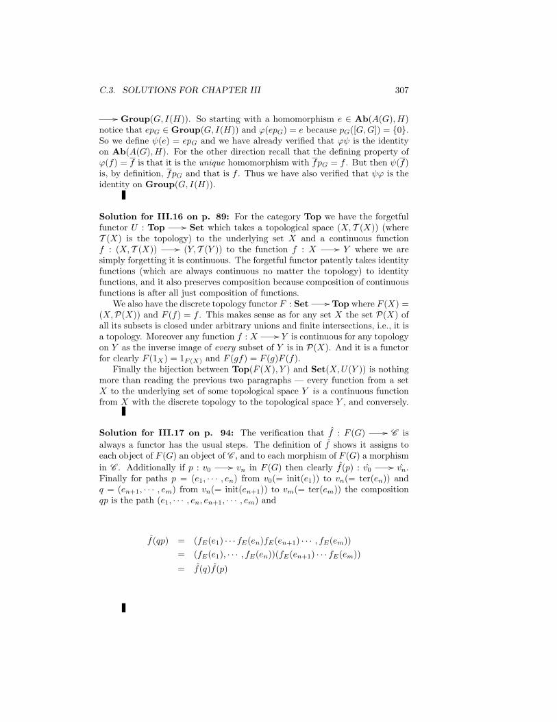
C.3. SOLUTIONS FOR CHAPTER III 307
// Group(G, I(H)). So starting with a homomorphism e ∈ Ab(A(G), H)notice that epG ∈ Group(G, I(H)) and ϕ(epG) = e because pG([G,G]) = 0.So we define ψ(e) = epG and we have already verified that ϕψ is the identityon Ab(A(G), H). For the other direction recall that the defining property ofϕ(f) = f is that it is the unique homomorphism with fpG = f . But then ψ(f)is, by definition, fpG and that is f . Thus we have also verified that ψϕ is theidentity on Group(G, I(H)).
Solution for III.16 on p. 89: For the category Top we have the forgetfulfunctor U : Top // Set which takes a topological space (X, T (X)) (whereT (X) is the topology) to the underlying set X and a continuous functionf : (X, T (X)) // (Y, T (Y )) to the function f : X // Y where we aresimply forgetting it is continuous. The forgetful functor patently takes identityfunctions (which are always continuous no matter the topology) to identityfunctions, and it also preserves composition because composition of continuousfunctions is after all just composition of functions.
We also have the discrete topology functor F : Set // Top where F (X) =(X,P(X)) and F (f) = f . This makes sense as for any set X the set P(X) ofall its subsets is closed under arbitrary unions and finite intersections, i.e., it isa topology. Moreover any function f : X // Y is continuous for any topologyon Y as the inverse image of every subset of Y is in P(X). And it is a functorfor clearly F (1X) = 1F (X) and F (gf) = F (g)F (f).
Finally the bijection between Top(F (X), Y ) and Set(X,U(Y )) is nothingmore than reading the previous two paragraphs — every function from a setX to the underlying set of some topological space Y is a continuous functionfrom X with the discrete topology to the topological space Y , and conversely.
Solution for III.17 on p. 94: The verification that f : F (G) // C isalways a functor has the usual steps. The definition of f shows it assigns toeach object of F (G) an object of C , and to each morphism of F (G) a morphismin C . Additionally if p : v0
// vn in F (G) then clearly f(p) : v0// vn.
Finally for paths p = (e1, · · · , en) from v0(= init(e1)) to vn(= ter(en)) andq = (en+1, · · · , em) from vn(= init(en+1)) to vm(= ter(em)) the compositionqp is the path (e1, · · · , en, en+1, · · · , em) and
f(qp) = (fE(e1) · · · fE(en)fE(en+1) · · · , fE(em))= (fE(e1), · · · , fE(en))(fE(en+1) · · · fE(em))
= f(q)f(p)

308 APPENDIX C. SOLUTIONS OF EXERCISES
Solution for III.18 on p. 94: The exercise here is to prove that the function
Digraph(G,U(C )) // Cat(F (G),C )
f 7→ f
is a bijection.The inverse function takes a functor k : F (G) // C to the digraph homo-
morphism k : G // C that just forgets about composition, i.e., kV (v) = k(v)and kE(e) = k(e). That k is a digraph homomorphism is an immediate con-sequence of the properties in the definition of a functor not involving compo-sition. The computation of ˇ
f is also immediate: ˇfV (v) = f(v) = fV (v) and
ˇfE(e)f(e) = fE(e), so ˇ
f = f . Also if g : C // D is any morphism in C , thenˆk(C) = kV (C) = k(C) and ˆk(g) = kE(f) = k(g). so ˆk = k.
Solution for III.19 on p. 96: In the terminology of the preceding exer-cise, the canonical functor ε : F (U(2)) // 2 is 1U(2), and we will use thedescription found above.
The category 2 has the two objects 0 and 1, the two identity morphisms 0, 1(with the same names as their corresponding objects) and the one non-identitymorphism ! : 0 // 1 (so named because it is the unique morphism from theinitial object 0 to the final object 1.) The underlying graph U(2) has the twonodes 0 and 1 and the three edges: 0 from 0 to 0; 1 from 1 to 1 and ! from 0to 1. So F (U(2)) has the two objects 0 and 1 and as morphisms all sequencesof the following forms:
1. an empty path on 0
2. ! as a path from 0 to 1
3. an empty path on 1
4. any path of positive length starting and ending at 0: (0, · · · , 0)
5. any path of positive length starting and ending at 1: (1, · · · , 1)
6. the other paths from 0 to 1: (0, · · · , 0, !, 1, · · · , 1)
From the above description we know that ε = 1U(2) takes the objects 0 to0 and 1 to 1, while on the morphisms it takes every path starting and endingat 0 to the identity morphism 0, every path starting and ending at 1 to theidentity morphism 1, and every path from 0 to 1 to the morphism !.
Solution for III.20 on p. 96: In order to describe in more detail the freecategory generated by the following digraph we have added names for the five
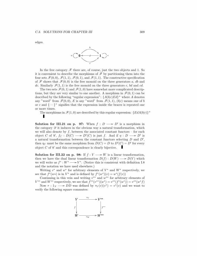
C.3. SOLUTIONS FOR CHAPTER III 309
edges.
0a$$
1 edd0 1
b
0 1oo d0 1
c
??
In the free category F there are, of course, just the two objects and 1. Soit is convenient to describe the morphisms of F by partitioning them into thefour sets F (0, 0), F (1, 1), F (0, 1), and F (1, 1). The constructive specificationof F shows that F (0, 0) is the free monoid on the three generators a, db anddc. Similarly F (1, 1) is the free monoid on the three generators e, bd and cd.
The two sets F (0, 1) and F (1, 0) have somewhat more complicated descrip-tions, but they are very similar to one another. A morphism in F (0, 1) can bedescribed by the following “regular expression”: A(b|c)Ed+ where A denotesany ”word” from F (0, 0), E is any ”word” from F (1, 1), (b|c) means one of bor c and · · · + signifies that the expression inside the braces is repeated oneor more times.
The morphisms in F (1, 0) are described by this regular expression: EdA(b|c)+
Solution for III.21 on p. 97: When f : D // D′ is a morphism inthe category D it induces in the obvious way a natural transformation, whichwe will also denote by f , between the associated constant functors – for eachobject C of C , fC : D(C) // D′(C) is just f . And if η : D // D′ isa natural transformation between the constant functors selecting D and D′,then ηC must be the same morphism from D(C) = D to D′(C) = D′ for everyobject C of C and this correspondence is clearly bijective.
Solution for III.22 on p. 98: If f : V // W is a linear transformation,then we have the dual linear transformation D(f) : D(W ) // D(V ) whichwe will write as f∗ : W ∗ // V ∗. (Notice this is consistent with definition I.8and the notation we have used elsewhere.)
Writing v∗ and w∗ for arbitrary elements of V ∗ and W ∗ respectively, wesee that f∗(w∗) is in V ∗ and is defined by f∗(w∗)(v) = w∗(f(v))
Continuing in this vein and writing v∗∗ and w∗∗ for arbitrary elements ofV ∗∗ and W ∗∗ respectively, we see that f∗∗(v∗∗)(w∗) = v∗∗(f∗(w∗)) = v∗∗(w∗f)
Now τ : 1V// DD was defined by τV (v)(v∗) = v∗(v) and we want to
verify the following square commutes:
W W ∗∗τW//
V
W
f
V V ∗∗τV // V ∗∗
W ∗∗
f∗∗

310 APPENDIX C. SOLUTIONS OF EXERCISES
Checking we see
(f∗∗τV )(v)(w∗) = f∗∗(τV (v))(w∗)= τV (v)(f∗(w∗))= τV (v)(w∗f)= (w∗f)(v)= w∗(f(v))= τW (f(v))(w∗)= (τW f)(v)(w∗)
The result that τV : V // V ∗∗ is always injective requires a bit of specialknowledge about vector spaces, to wit the result that if v is any non-zeroelement of V , then there exists an element v∗ of V ∗ with v∗(v) 6= 0. This isusually proved using the observation that every non-zero v is part of a basisfor V , for then if B is such a basis we can define v∗(Σb∈Bcbb) = cv with cv thecoefficient of v ∈ V . For that we see that if τV (v) = 0, then τV (v)(v∗) = 0 forall v∗ ∈ V ∗ which by the above observation implies v = 0.
Solution for III.23 on p. 98: Recall (cf. Section III.2.12) the construc-tion of the free monoid F (S) on the set S as the set of finite sequence ofelements of S with the binary operation of concatenation. For f : S // Tthe homomorphism F (f) : F (S) // F (T ) is given by F (f)(s0, · · · , sn) =(f(s0), · · · , f(sn)).
The natural transformation η : 1Set// UF is defined as ηS(s) = (s)
with (s) the sequence with just one term, s. To verify that η is a naturaltransformation we must show that the following diagram always commutes.
T UF (T )ηT//
S
T
f
S UF (S)ηS // UF (S)
UF (T )
UF (f)
With all of this the actual verification is immediate:
UF (f)(ηS(s)) = UF (f)((s)) = (f(s))ηT (f(s)) = (f(s))
Solution for III.24 on p. 99: The natural transformation ε : FU //
1Monoid is defined by εM (m1,m2, · · · ,mn) = m1m2 · · ·mn To verify that εis a natural transformation we must show that the following diagram always

C.3. SOLUTIONS FOR CHAPTER III 311
commutes:
FU(N) NεN//
FU(M)
FU(N)
FU(f)
FU(M) MεM // M
N
f
That is just the following simple calculation:
f(εM (m1,m2, · · · ,mn)) = f(m1m2 · · ·mn) = f(m1)f(m2) · · · f(mn)εN (FU(f)((m1m2 · · ·mn))) = εN ((f(m1)f(m2) · · · f(mn))) = f(m1)f(m2) · · · f(mn)
Solution for III.25 on p. 99: In Section III.2.12 we defined a func-tion from Set(A,U(M)) to Monoid(F (A),M) by assigning to each f : A
// U(M) the monoid homomorphism f∗ : A∗ // M with f∗(()) = 1 andf∗(a1, a2, · · · , an) = f(a1)f(a2) · · · f(an)
Now we also have the function Set(A,U(M)) // Monoid(F (A),M)given by f 7→ εMF (f) where ε : FU // 1Monoid is defined as εM (m1,m2, · · · ,mn) =m1m2 · · ·mn, and this exercise is to verify that these are the same functions.The verification consists of explicitly evaluating εMF (f): εM (F (f)(a1, a2, · · · , an)) =εM (f(a1), f(a2), · · · , f(an)) = f(a1)f(a2) · · · f(an)
Solution for III.26 on p. 99: As a preliminary step, if we consider thefunction Monoid(F (A),M) // Set(A,U(M)) given by h 7→ U(h)η andwrite h for U(h)η we immediately see that h(a) = h(a). [Beware of the changeof type between the two occurrences of a – the first is a as an element of theset A, while the second is actually a as the single element in the one elementsequence (a).]
Combining this observation with the immediately preceding exercise we seethat the composition
Set(A,U(M)) // Monoid(F (A),M) // Set(A,U(M))
assigns to a function f the function f∗ and f∗(a) is just f(a), i.e., f∗ = f .Similarly the composition
Monoid(F (A),M) // Set(A,U(M)) // Monoid(F (A),M)
assigns to a homomorphism h the homomorphism h∗ and h∗(s) is just h(s),i.e., h∗ = h. So the function Monoid(F (A),M) // Set(A,U(M)) givenby h 7→ U(h)η is the inverse of the function of the preceding exercise.
The above verification is as simple and direct as can be imagined, butthere is a little more complex approach which has the advantage of connectingdirectly with the general study of adjunctions and adjoint functors, so we offerit as well.

312 APPENDIX C. SOLUTIONS OF EXERCISES
First observe that
F (A)F (ηA) // FUF (A)
εF (A) // F (A)U(M)
ηU(M)// UFU(M)
U(εM )// U(M)
are immediately verified to be identity morphisms. Next note that the compo-sition:
Set(A,U(M)) // Monoid(F (A),M) // Set(A,U(M))
assigns to a function f the following composite function.
F (A) FUF (A)F (ηA) // FUF (A) FU(M)
FU(h) // FU(M)
M
εM
Adding a few more morphisms gives the following diagram as ε is a naturaltransformation.
F (A) FUF (A)F (ηA) // FUF (A) FU(M)
FU(h) //F (A)
F (A)
1F (A)
''OOOOOOOOOOOOOOOO FUF (A)
F (A)
εF (A)
FU(M)
M
εM
F (A) M
h //
Of course this says exactly that going from Set(A,U(M)) to Monoid(F (A),M)and back to Set(A,U(M)) is the identity.
In much the same way the following commutative diagram shows that goingfrom Monoid(F (A),M) to Set(A,U(M)) and back to Monoid(F (A),M) isthe identity.
UF (A) UFU(M)UF (f) // UFU(M) U(M)
U(εM ) //
A
UF (A)
ηA
OO
U(M)
UFU(M)
ηU(M)
OO
U(M)
U(M)
1U(M)
77ooooooooooooooooA U(M)
f //
Solution for III.27 on p. 99: The natural transformation φA,M : Set(A,U(M))// Monoid(F (A),M) is defined by φA,M (f) = εMF (f), while the natural
transformation ψA,M : Monoid(F (A),M) // Set(A,U(M)) is defined byψA,M (h) = U(h)ηA. By the last exercise these are inverse functions, so the

C.3. SOLUTIONS FOR CHAPTER III 313
only work required to verify that they give a natural isomorphism is to verifythat they are in fact natural transformations, which means verifying that forall morphisms f : A // B and h : M // N the following diagrams arecommutative.
Set(B,U(N)) Monoid(F (B), N)φB,N
//
Set(A,U(M))
Set(B,U(N))
(f,U(h))∗
Set(A,U(M)) Monoid(F (A),M)φA,M // Monoid(F (A),M)
Monoid(F (B), N)
(F (f),h)∗
Monoid(F (B), N) Set(B,U(N))ψB,N
//
Monoid(F (A),M)
Monoid(F (B), N)
(F (f),h)∗
Monoid(F (A),M) Set(A,U(M))ψA,M // Set(A,U(M))
Set(B,U(N))
(f,U(h))∗
For the first diagram, notice that the result of starting with b ∈ Set(A,U(M))and following it across the top and down on the right is hεMF (b)F (f) while theresult of going down on the left and across the bottom is εNFU(h)F (b)F (f).As ε is a natural transformation we know that εNFU(h) = hεM and so thediagram is commutative.
For the second diagram, notice that the result of starting with k ∈Monoid(F (A),M)and following it across the top and down on the right is U(h)U(k)ηAf while theresult of going down on the left and across the bottom is U(h)U(k)UF (f)ηA.As η is a natural transformation we know that ηAf = UF (f)ηA and so thediagram is commutative.
Solution for III.28 on p. 100: Verification that inclusion of the commutatorsubgroup into the containing group is a natural transformation is just a matterof displaying the relevant diagram:
[H,H] Hιh//
[G,G]
[H,H]
f |[H,H]
[G,G] GιG // G
H
f
Solution for III.29 on p. 100: Verification that projection onto the abelian-izer of a group is a natural transformation is just a matter of displaying the

314 APPENDIX C. SOLUTIONS OF EXERCISES
relevant diagram:
H H/[H,H]πH//
G
H
f
G G/[G,G]πG // G/[G,G]
H/[H,H]
f
Solution for III.30 on p. 100: This is one of those cases where the formalismcomplicates a very simple situation. The bijection between Ab(A(G), A) andGroup(G, I(A)) is just the simple observation that any group homomorphismfrom an arbitrary group G into an Abelian group factors uniquely throughA(G) as group homomorphisms preserve commutators and every commutatorin a Abelian group is the identity.
Solution for III.31 on p. 100: Verification that Ab(A(•), •) is naturallyequivalent to Group(•, I(•)) just consists of showing that the functions dis-cussed in the last exercise are actually natural transformations, which meansverifying that for all morphisms f : H // F and h : A // B the followingsquares are commutative.
Ab(A(H), B) Group(H, I(B))φH,B
//
Ab(A(G), A)
Ab(A(H), B)
(A(f),h)∗
Ab(A(G), A) Group(G, I(A))φG,A // Group(G, I(A))
Group(H, I(B))
(f,I(h))∗
] ]
Group(H, I(B)) Ab(A(H), B)ψH,B
//
Group(G, I(A))
Group(H, I(B))
(f,I(h))∗
Group(G, I(A)) Ab(A(G), A)ψG,A // Ab(A(G), A)
Ab(A(H), B)
(A(f),h)∗
] ]
φG,AShow that Ab(A(•), •) is naturally equivalent to Group(•, I(•)) with both
considered as functors from Groupop ×Ab to Set.
Solution for III.32 on p. 101: Verify that ε : FU // 1Top is indeed anatural transformation.
Solution for III.33 on p. 101: Show that the two functions just de-fined are inverse to one another and give bijections between Top(F (S), X)and Set(S,U(X)).

C.4. SOLUTIONS FOR CHAPTER IV 315
Solution for III.34 on p. 101: Show that Top(F (•), •) is naturally iso-morphic to Set(•, I(•)) with both considered as functors from Setop×Top toSet.
Solution for III.35 on p. 102: Verify that βF as just defined is indeed anatural transformation from GF to G′F .
Solution for III.36 on p. 102: Verify that Gα as just defined is indeed anatural transformation from GF to GF ′.
Solution for III.37 on p. 103: Show that for any category C the functorcategory C 1 is isomorphic to C
Hint: Every functor 1 // C takes the unique object in 1 to an objectin C , and that completely determines the functor, so all that is left is to notethat a natural transformation between such functors is the same as a morphismbetween the objects.
Solution for III.38 on p. 103: If D is a discrete finite category with nobjects, show that C D ∼= C n where C n is the n-fold product of C with itself.
C.4 Solutions for Chapter IV
C.5 Solutions for Chapter V
Solution for V.5 on p. 144:To see that the equation (Uη)(εU) = 1U implies θξ is the identity on
(S ↓ U), observe that the result of applying θξ toExtend this to the following larger commutative diagram by adding the dot-
ted arrows shown using the naturality of η and the assumption that (ηF )(Fε) =1F
UF (S) UF (S′)//
S
UF (S)
εS
S S′s // S′
UF (S′)
εS′ )
S
S
1S
yy
U(M) UFU(M)εU(M)//
S
U(M)
g
S UF (S)εS // UF (S)
UFU(M)
UF (S)
UFU(M)U(M)
U(M)
1U(M)
%%
UFU(M) UFU(M ′)//
UF (S)
UFU(M)
UF (g)
UF (S) UF (S′)UF (s) // UF (S′)
UFU(M ′)
UF (g′)
S′
S′
1S′
%%
UFU(M ′) U(M ′)εU(M′)//
UF (S′)
UFU(M ′)
UF (S′)
UFU(M ′)
UF (S′) S′εS′ // S′
U(M ′)
g′
U(M ′)
U(M ′)
1U(M′)
yyU(M) U(M ′)
U(m)//
UFU(M)
U(M)
U(ηM )
UFU(M) UFU(M ′)UFU(m)// UFU(M ′)
U(M ′)
U(ηM′ )
and this gives the result.

316 APPENDIX C. SOLUTIONS OF EXERCISES
C.6 Solutions for Chapter VII
C.7 Solutions for Chapter VIII
C.8 Solutions for Chapter XIII
C.9 Solutions for Chapter XIV
C.10 Solutions for Chapter IX
C.11 Solutions for Chapter VI
Solution for VI.1 on p. 147: Verify that if the product C × C exists, thend0, d1 are jointly monic iff 〈d0, d1〉 : R // C × C is monic.
Solution for VI.2 on p. 148: Suppose that in C the pair d0, d1 : R // C isa relation on C. Show that it is a reflexive relation iff Hom(X, d0),Hom(X, d1) :Hom(X,R) // Hom(X,C) is a reflexive relation in Set.
C.12 Solutions for Appendix B
Solution for B.1 on p. 253: Suppose P is a small category with theproperty that for any two objects A and B of P there is at most one morphismfrom A to B. Define a relation on the objects of P by A B iff there is amorphism from A to B. Demonstrate that the set of objects of P with therelation is a partially ordered set. Similarly if
Solution for B.2 on p. 254: To prove that 1 + 1 = 1 in 2, note that thereis only one morphism with domain 1, namely the identity, and it serves asthe unique morphism from 1 + 1 to 1. In the same fashion there is only onemorphism with codomain 0, namely the identity, and it serves as the uniquemorphism from 0 to 0× 0 = 0.

Appendix D
Other Sources
Even though category theory is a relatively young part of mathematics, it hasa huge literature. In particular there are a many accounts of the materialin these notes, and the study of category theory benefits from this variety ofperspectives. Here are listed a number of generally available books and notes,together with some brief comments on them. In particular all of these havebeen useful in preparing these notes.
317

318 APPENDIX D. OTHER SOURCES
D.1 Introductions
D.1.1 Abstract and Concrete Categories: The Joy of Cats(Adamek, Herrlich, and Strecker [?])
0 Introduction1 Motivation2 Foundations
I Categories, Functors, and Natural Transformations3 Categories and functors4 Subcategories5 Concrete categories and concrete functors6 Natural transformations
II Objects and Morphisms7 Objects and morphisms in abstract categories8 Objects and morphisms in concrete categories9 Injective objects and essential embeddings
III Sources and Sinks10 Sources and sinks11 Limits and colimits12 Completeness and cocompleteness13 Functors and limits
IV Factorization Structures14 Factorization structures for morphisms15 Factorization structures for sources16 E-reflective subcategories17 Factorization structures for functors
V Adjoints and Monads18 Adjoint functors19 Adjoint situations20 Monads
VI Topological and Algebraic Categories21 Topological categories22 Topological structure theorems23 Algebraic categories24 Algebraic structure theorems25 Topologically algebraic categories26 Topologically algebraic structure theorems
VII Cartesian Closedness and Partial Morphisms27 Cartesian closed categories28 Partial morphisms, quasitopoi, and topological universesTables
Functors and morphisms: Preservation propertiesFunctors and morphisms: Reflection propertiesFunctors and limitsFunctors and colimitsStability properties of special epimorphisms
Table of CategoriesTable of Symbols
D.1.2 Category Theory (Awodey [?])1 Categories
1.1 Introduction1.2 Functions of sets1.3 Definition of a category1.4 Examples of categories1.5 Isomorphisms1.6 Constructions on categories1.7 Free categories1.8 Foundations: large, small, and locally small1.9 Exercises
2 Abstract structures2.1 Epis and monos2.2 Initial and terminal objects

D.1. INTRODUCTIONS 319
2.3 Generalized elements2.4 Sections and retractions2.5 Products2.6 Examples of products2.7 Categories with products2.8 Hom-sets2.9 Exercises
3 Duality3.1 The duality principle3.2 Coproducts3.3 Equalizers3.4 Coequalizers3.5 Exercises
4 Groups and categories4.1 Groups in a category4.2 The category of groups4.3 Groups as categories4.4 Finitely presented categories4.5 Exercises
5 Limits and colimits5.1 Subobjects5.2 Pullbacks5.3 Properties of pullbacks5.4 Limits5.5 Preservation of limits5.6 Colimits5.7 Exercises
6 Exponentials6.1 Exponential in a category6.2 Cartesian closed categories6.3 Heyting algebras6.4 Equational definition6.5 λ-calculus6.6 Exercises
7 Functors and naturality7.1 Category of categories7.2 Representable structure7.3 Stone duality7.4 Naturality7.5 Examples of natural transformations7.6 Exponentials of categories7.7 Functor categories7.8 Equivalence of categories7.9 Examples of equivalence
7.10 Exercises8 Categories of diagrams
8.1 Set-valued functor categories8.2 The Yoneda embedding8.3 The Yoneda Lemma8.4 Applications of the Yoneda Lemma8.5 Limits in categories of diagrams8.6 Colimits in categories of diagrams8.7 Exponentials in categories of diagrams8.8 Topoi8.9 Exercises
9 Adjoints9.1 Preliminary definition9.2 Hom-set definition9.3 Examples of adjoints9.4 Order adjoints9.5 Quantifiers as adjoints9.6 RAPL9.7 Locally cartesian closed categories9.8 Adjoint functor theorem9.9 Exercises
10 Monads and algebras10.1 The triangle identities10.2 Monads and adjoints

320 APPENDIX D. OTHER SOURCES
10.3 Algebras for a monad10.4 Comonads and coalgebras10.5 Algebras for endofunctors10.6 Exercises
D.1.3 Category Theory: An Introduction (Herrlich andStrecker [?])
I IntroductionII Foundations
1 Set, classes and conglomeratesIII Categories
2 Concrete categories3 Abstract categories4 New categories from old
IV Special Morphisms and Special Objects5 Sections, retractions and isomorphisms6 Monomorphisms, epimorphisms, and bimorphisms7 Initial, terminal, and zero objects8 Constant morphisms, zero morphisms, and pointed categories
V Functors and Natural Transformations9 Functors
10 Hom-functors11 Categories of categories12 Properties of functors13 Natural transformations and natural isomorphisms14 Isomorphisms and equivalences of categories15 Functor categories
VI Limits in Categories16 Equalizers and coequalizers17 Intersections and factorizations18 Products and coproducts19 Sources and sinks20 Limits and colimits21 Pullbacks and pushouts22 Inverse and direct limits23 Complete categories24 Functors that preserve and reflect limits25 Limits in functor categories
VII Adjoint Situations26 Universal maps27 Adjoint functors28 Existence of adjoints
VIII Set-Valued Functors29 Hom-functors30 Representable functors31 Free objects32 Algebraic categories and algebraic functors
IX Subobjects, Quotient Objects, and Factorizations33 (E , M ) categories34 (Epi, extremal mono) and (extremal epi, mono) categories35 (Generating, extremal mono) and (extremal generating, mono) factorizations
X Reflective Subcategories36 General reflective subcategories37 Characterization and generation of E -reflective subcategories38 Algebraic subcategories
XI Pointed Categories39 Normal and exact categories40 Additive categories41 Abelian categories
Appendix: Foundations
D.1. INTRODUCTIONS 321
D.1.4 Arrows, Structures, and Functors: The CategoricalImperative (Arbib and Manes [1])
PART IChapter 1 Learning to Think with Arrows
1.1 Epimorphisms and Monomorphisms1.2 Products and Coproducts1.3 Coequalizers and Equalizers
Chapter 2 Basic Concepts of Category Theory2.1 Vector Spaces and Posets2.2 The Definition of a Category2.3 Epimorphisms and Monomorphisms2.4 Limits and Colimits
Chapter 3 Monoids and Groups3.1 Defining the Categories3.2 Constructions within the Categories
Chapter 4 Metric and Topological Spaces4.1 Categories of Metric Spaces4.2 Constructions in Categories of Metric Spaces4.3 Topological Spaces
Chapter 5 Additive Categories5.1 Vectors and Matrices in a Category5.2 Abm-Categories
Chapter 6 Structured Sets6.1 The Admissible Maps Approach to Structure6.2 Optimal Families6.3 Examples from Automata Theory
Part IIChapter 7 Functors and Adjoints
7.1 Functors7.2 Free and Cofree7.3 Natural Transformations and Adjunctions
Chapter 8 The Adjoint Functor Theorem8.1 Necessary Conditions8.2 Sufficient Conditions
Chapter 9 Monoidal and Closed Categories9.1 Motivation from Set Theory9.2 Monoids in a Monoidal Category9.3 Categories over a Monoidal Category9.4 The Godement Calculus
Chapter 10 Monads and Algebras10.1 Universal Algebra10.2 From Monoids to Monads10.3 Monads from Free Algebras
D.1.5 Category Theory: Lecture Notes for ESSLLI (Barrand Wells [?])
1. Preliminaries1.1 Graphs1.2 Homomorphisms of graphs
2. Categories2.1 Basic definitions2.2 Functional programming languages as categories2.3 Mathematical structures as categories2.4 Categories of sets with structure2.5 Categories of algebraic structures2.6 Constructions on categories
3. Properties of objects and arrows3.1 Isomorphisms3.2 Terminal and initial objects3.3 Monomorphisms and subobjects3.4 Other types of arrow
4. Functors4.1 Functors4.2 Actions

322 APPENDIX D. OTHER SOURCES
4.3 Types of functors4.4 Equivalences
5. Diagrams and naturality5.1 Diagrams5.2 Natural transformations5.3 Natural transformations between functors5.4 Natural transformations involving lists5.5 Natural transformations of graphs5.6 Combining natural transformations and functors5.7 The Yoneda Lemma and universal elements
6. Products and sums6.1 The product of two objects in a category6.2 Notation for and properties of products6.3 Finite products6.4 Sums6.5 Deduction systems as categories
7. Cartesian closed categories7.1 Cartesian closed categories7.2 Properties of cartesian closed categories7.3 Typed λ-calculus7.4 λ-calculus to category and back
8. Limits and colimits8.1 Equalizers8.2 The general concept of limit8.3 Pullbacks8.4 Coequalizers8.5 Cocones
9. Adjoints9.1 Free monoids9.2 Adjoints9.3 Further topics on adjoints
10. Triples10.1 Triples10.2 Factorization of a triple
11. Toposes11.1 Definition of topos11.2 Properties of toposes11.3 Presheaves11.4 Sheaves
12. Categories with monoidal structure12.1 Closed monoidal categories12.2 Properties of A ( C12.3 *-autonomous categories12.4 Factorization systems12.5 The Chu construction
D.1.6 Category Theory for Computing Science (Barr andWells [3])
1. Preliminaries1.1 Sets1.2 Functions1.3 Graphs1.4 Homomorphisms of graphs
2. Categories2.1 Basic definitions2.2 Functional programming languages as categories2.3 Mathematical structures as categories2.4 Categories of sets with structure2.5 Categories of algebraic structures2.6 Constructions on categories2.7 Properties of objects and arrows in a category2.8 Other types of arrow2.9 Factorization systems
3. Functors3.1 Functors

D.1. INTRODUCTIONS 323
3.2 Actions3.3 Types of functors3.4 Equivalences3.5 Quotient categories
4. Diagrams, naturality and sketches4.1 Diagrams4.2 Natural transformations4.3 Natural transformations between functors4.4 The Godement calculus of natural transformations4.5 The Yoneda Lemma and universal elements4.6 Linear sketches (graphs with diagrams)4.7 Linear sketches with constants: initial term models4.8 2-categories
5. Products and sums5.1 The product of two objects in a category5.2 Notation for and properties of products5.3 Finite products5.4 Sums5.5 Natural numbers objects5.6 Deduction systems as categories5.7 Distributive categories
6. Cartesian closed categories6.1 Cartesian closed categories6.2 Properties of cartesian closed categories6.3 Typed λ-calculus6.4 λ-calculus to category and back6.5 Arrows vs. terms6.6 Fixed points in cartesian closed categories
7. Finite product sketches7.1 Finite product sketches7.2 The sketch for semigroups7.3 Notation for FP sketches7.4 Arrows between models of FP sketches7.5 Signatures and FP sketches
8. Finite discrete sketches8.1 Sketches with sums8.2 The sketch for fields8.3 Term algebras for FD sketches
9. Limits and colimits9.1 Equalizers9.2 The general concept of limit9.3 Pullbacks9.4 Coequalizers9.5 Cocones9.6 More about sums9.7 Unification as coequalizer9.8 Properties of factorization systems
10. More about sketches10.1 Finite limit sketches10.2 Initial term models of FL sketches10.3 The theory of an FL sketch10.4 General definition of sketch
11. The category of sketches11.1 Homomorphisms of sketches11.2 Parameterized data types as pushouts11.3 The model category functor
12. Fibrations12.1 Fibrations12.2 The Grothendieck construction12.3 An equivalence of categories12.4 Wreath products
13. Adjoints13.1 Free monoids13.2 Adjoints13.3 Further topics on adjoints13.4 Locally cartesian closed categories
14. Algebras for endofunctors14.1 Fixed points for a functor

324 APPENDIX D. OTHER SOURCES
14.2 Recursive categories14.3 Triples14.4 Factorization of a triple14.5 Scott domains
15. Toposes15.1 Definition of topos15.2 Properties of toposes15.3 Presheaves15.4 Sheaves15.5 Fuzzy sets15.6 External functors15.7 The realizability topos
16. Categories with monoidal structure16.1 Closed monoidal categories16.2 Properties of A ( C16.3 *-autonomous categories16.4 Factorization systems16.5 The Chu construction
Solutions to the exercises
D.1.7 Categories (Blyth [8])Chapter 1 – Looking at the woods rather than the treesChapter 2 – Particular objects and morphismsChapter 3 – Universal constructionsChapter 4 – Factorisation of morphismsChapter 5 – Structuring the morphism setsChapter 6 – FunctorsChapter 7 – Equivalent categoriesChapter 8 – Representable and adjoint functors
D.1.8 Handbook of Categorical Algebra I: Basic CategoryTheory (Borceux [?])
1. The language of categories1.1 Logical foundations of the theory1.2 Categories and functors1.3 Natural transformations1.4 Contravariant functors1.5 Full and faithful functors1.6 Comma categories1.7 Monomorphisms1.8 Epimorphisms1.9 Isomorphisms
1.10 The duality principle1.11 Exercises
2. Limits2.1 Products2.2 Coproducts2.3 Initial and terminal objects2.4 Equalizers, coequalizers2.5 Pullbacks, pushouts2.6 Limits and colimits2.7 Complete categories2.8 Existence theorem for limits2.9 Limit preserving functors
2.10 Absolute colimits2.11 Final functors2.12 Interchange of limits2.13 Filtered colimits2.14 Universality of colimits2.15 Limits in categories of functors2.16 Limits in comma categories2.17 Exercises
3. Adjoint functors

D.1. INTRODUCTIONS 325
3.1 Reflection along a functor3.2 Properties of adjoint functors3.3 The adjoint functor theorem3.4 Fully faithful adjoint functors3.5 Reflective subcategories3.6 Epireflective subcategories3.7 Kan extensions3.8 Tensor product of set-valued functors3.9 Exercises
4. Generators and projectives4.1 Well-powered categories4.2 Intersection and union4.3 Strong epimorphisms4.4 Epi-mono factorizations4.5 Generators4.6 Projectives4.7 Injective cogenerators4.8 Exercises
5. Categories of fractions5.1 Graphs and path categories5.2 Calculus of fractions5.3 Reflective subcategories as categories of fractions5.4 The orthogonal subcategory problem5.5 Factorization systems5.6 The case of localizations5.7 Universal closure operations5.8 The calculus of bidense morphisms5.9 Exercises
6. Flat functors and Cauchy completeness6.1 Exact functors6.2 Left exact reflections of a functor6.3 Flat functors6.4 The relevance of regular cardinals6.5 The splitting of idempotents6.6 The more general adjoint functor theorem6.7 Exercises
7. Bicategories and distributors7.1 2-categories7.2 2-functors and 2-natural transformations7.3 Modifications and n-categories7.4 2-limits and bilimits7.5 Lax functors and pseudo-functors7.6 Bicategories7.7 Distributors7.8 Cauchy completeness versus distributors7.9 Exercises
8. Internal category theory8.1 Internal categories and functors8.2 Internal base-valued functors8.3 Internal limits and colimits8.4 Exercises
D.1.9 Handbook of Categorical Algebra II: (Borceux [?])1. Abelian categories
1.1 Zero objects and kernels1.2 Additive categories and biproducts1.3 Additive functors1.4 Abelian categories1.5 Exactness properties of abelian categories1.6 Additivity of abelian categories1.7 Union of subobjects1.8 Exact sequences1.9 Diagram chasing
1.10 Some diagram lemmas1.11 Exact functors1.12 Torsion theories

326 APPENDIX D. OTHER SOURCES
1.13 Localizations of abelian categories1.14 The embedding theorem1.15 Exercises
2. Regular categories2.1 Exactness properties of regular categories2.2 Definition in terms of strong epimorphisms2.3 Exact sequences2.4 Examples2.5 Equivalence relations2.6 Exact categories2.7 An embedding theorem2.8 The calculus of relations2.9 Exercises
3. Algebraic theories3.1 The theory of groups revisited3.2 A glance at universal algebra3.3 A categorical approach to universal algebra3.4 Limits and colimits in algebraic categories3.5 The exactness properties of algebraic categories3.6 The algebraic lattice of subobjects3.7 Algebraic functors3.8 Finitely generated models3.9 Characterization of algebraic categories
3.10 Commutative theories3.11 Tensor product of theories3.12 A glance at Morita theory3.13 Exercises
4. Monads4.1 Monads and their algebras4.2 Monads and adjunctions4.3 Limits and colimits in categories of algebras4.4 Characterization of monadic categories4.5 The adjoint lifting theorem4.6 Monads with rank4.7 A glance at descent theory4.8 Exercises
5. Accessible categories5.1 Presentable objects in a category5.2 Locally presentable categories5.3 Accessible categories5.4 Raising the degree of accessibility5.5 Functors with rank5.6 Sketches5.7 Exercises
6. Enriched category theory6.1 Symmetric monoidal closed categories6.2 Enriched categories6.3 The enriched Yoneda lemma6.4 Change of base6.5 Tensors and cotensors6.6 Weighted limits6.7 Enriched adjunctions6.8 Exercises
7. Topological categories7.1 Exponentiable spaces7.2 Compactly generated spaces7.3 Topological functors7.4 Exercises
8. Fibred categories8.1 Fibrations8.2 Cartesian functors8.3 Fibrations via pseudo-functors8.4 Fibred adjunctions8.5 Completeness of a fibration8.6 Locally small fibrations8.7 Definability8.8 Exercises

D.1. INTRODUCTIONS 327
D.1.10 Handbook of Categorical Algebra III: (Borceux [?])
1. Locales1.1 The intuitionistic propositional calculus1.2 Heyting algebras1.3 Locales1.4 Limits and colimits of locales1.5 Nuclei1.6 Open morphisms of locales1.7 Etale morphisms of locales1.8 The points of a locale1.9 Sober spaces
1.10 Compactness conditions1.11 Regularity conditions1.12 Exercises
2. Sheaves2.1 Sheaves on a locale2.2 Closed subobjects2.3 Some categorical properties of sheaves2.4 Etale spaces2.5 The stalks of a topological sheaf2.6 Associated sheaves and etale morphisms2.7 Systems of generators for a sheaf2.8 The theory of Ω-sets2.9 Complete Ω-sets
2.10 Some basic facts in ring theory2.11 Sheaf representation of a ring2.12 Change of base2.13 Exercises
3. Grothendieck toposes3.1 A categorical glance at sheaves3.2 Grothendieck topologies3.3 The associated sheaf functor theorem3.4 Categorical properties of Grothendieck toposes3.5 Localization of Grothendieck toposes3.6 Characterization of Grothendieck toposes3.7 Exercises
4. The classifying topos4.1 The points of a topos4.2 The classifying topos of a finite limit theory4.3 The classifying topos of a geometric sketch4.4 The classifying topos of a coherent theory4.5 Diaconescu’s theorem4.6 Exercises
5. Elementary toposes5.1 The notion of a topos5.2 Examples of toposes5.3 Monomorphisms in a topos5.4 Some set theoretical notions in a topos5.5 Partial morphisms5.6 Injective objects5.7 Finite colimits5.8 The slice toposes5.9 Exactness properties of toposes
5.10 Union of subobjects5.11 Morphisms of toposes5.12 Exercises
6. Internal logic of a topos6.1 The language of a topos6.2 Categorical foundations of the logic of toposes6.3 The calculus of truth tables6.4 The point about “ghost” variables6.5 Coherent theories6.6 The Kripke-Joyal semantics6.7 The intuitionistic propositional calculus in a topos6.8 The intuitionistic predicate calculus in a topos6.9 Intuitionistic set theory in a topos
6.10 The structure of a topos in its internal language

328 APPENDIX D. OTHER SOURCES
6.11 Locales in a topos6.12 Exercises
7. The law of excluded middle7.1 The regular elements of Ω7.2 Boolean toposes7.3 De Morgan toposes7.4 Decidable objects7.5 The axiom of choice7.6 Exercises
8. The axiom of infinity8.1 The natural number object8.2 Infinite objects in a topos8.3 Arithmetic in a topos8.4 Finite objects in a topos8.5 Exercises
9. Sheaves in a topos9.1 Topologies in a topos9.2 Sheaves for a topology9.3 The localization of a topos9.4 The double negation sheaves9.5 Exercises
D.1.11 Introduction to the Theory of Categories andFunctors (Bucur and Deleanu [?])
1 Basic concepts1 The Notion of a Category. Duality. Subcategories. Examples2 Monomorphisms, epimorphisms, isomorphisms3 Functors4 Representable functors5 Adjoint functors6 The notion of equivalence between categories
2 Sum and products1 Direct sums and products2 Kernel and cokernel3 Grothendieck topologies and the general notion of a sheaf
3 Inductive and projective limits1 The general notion of a projective or inductive limit2 Existence of inductive or projective limits3 Commutation of functors with projective and inductive limits4 Characterization of adjoint functors5 Prorepresentable functors
4 Structures on the objects of a category1 Algebraic operations on the objects of a category. Homomorphisms2 The existence of kernels for homomorphisms3 Equivalence relations4 The general notion of a structure on the objects of a category
5 General theory of Abelian categories1 Additive categories2 Kernel and cokernel3 The canonical factorization of a morphism4 Pre-Abelian categories5 Abelian categories6 Exact functors7 The isomorphism theorems in Abelian categories8 The conditions AB3, AB4, AB59 Generators
10 Full embedding of a small Abelian category into a Grothendieck category6 Injective and projective objects in Abelian categories
1 The notion of an injective (projective) object and its general properties2 Essential extensions3 Properties of injective envelopes4 Projective objects5 Localization in rings6 Characterization of Grothendieck categories7 The theorem of Krull-Remak-Schmidt
D.1. INTRODUCTIONS 329
8 The structure of injective objects in locally Noetherian categories9 Applications to the decomposition theories
7 Elements of homological algebra1 Complexes, homology, cohomology2 Resolutions3 Derived functors4 Other properties of derived functors5 Homology and cohomology functors6 Other properties of homology and cohomology functors7 The homological dimension of Abelian categories8 Minimal projective resolutions9 Relative homological algebra
D.1.12 Lecture Notes in Category Theory (Caccamo [?])1. Categories, Functors and Natural Transformations
a) Categoriesb) Functorsc) Natural Transformationsd) Functor Categories
2. Constructions on Categoriesa) Opposite Category and Contravarianceb) Product of Categoriesc) Natural Transformations between Bifunctorsd) Examples
3. Yoneda Lemma and Universal Propertiesa) Yoneda Lemmab) Representability
4. Limits and Colimitsa) Definition of Limitsb) Examples of Limitsc) Limits in Setd) Limits as Products and Equalizerse) Definition of Colimitf) Examples of Colimitsg) Colimits in Seth) Limits with Parameters
5. Endsa) Dinaturalityb) Special Cases of Dinatural Transformationsc) Definition of Endd) Ends in Sete) Ends with Parameters
6. Limits and Endsa) Some Useful Isomorphismsb) Limits in Functor Categoriesc) Fubini Theoremd) Preservation of Limits
7. Preservation of Limitsa) Definitionb) Connected Diagramsc) Productsd) General Limits
8. Coendsa) Definition of Coendb) Density Formulac) Recasting the Density Formula
9. Adjunctionsa) Definition of Adjunctionsb) The Naturality Laws for Adjunctionsc) The Triangle Identitiesd) Limits and Adjunctionse) Representation Functorsf) Adjoints and Initial Objectsg) The Initial Object Lemmah) The General Adjoint Functor Theoremi) Well-powered categories

330 APPENDIX D. OTHER SOURCES
j) The Special Adjoint Functor Theoremk) Cartesian-closed Categories
D.1.13 Abelian Categories: An Introduction to the Theoryof Functors (Freyd [?])IntroductionExercises on Extremal CategoriesExercises on Typical Categories
CH1PTER 1. FUNDAMENTALS1.1 Contravariant Functors and Dual Categories1.2 Notation1.3 The Standard Functors1.4 Special Maps1.5 Subobjects and Quotient Objects1.6 Difference Kernels and Cokernels1.7 Products and Sums1.8 Complete Categories1.9 Zero Objects, Kernels, and Cokernels
CH2PTER 2. FUNDAMENTALS OF ABELIAN CATEGORIES2.1 Theorems for Abelian Categories2.2 Exact Sequences2.3 The Additive Structure for Abelian Categories2.4 Recognition of Direct Sum Systems2.5 The Pullback and Pushout Theorems2.6 Classical Lemmas
CH3PTER 3. SPECIAL FUNCTORS AND SUBCATEGORIES3.1 Additivity and Exactness3.2 Embeddings3.3 Special Objects3.4 Subcategories3.5 Special Contravariant Functors3.6 Bifunctors
CH4PTER 4. METATHEOREMS4.1 Very Abelian Categories4.2 First Metatheorem4.3 Fully Abelian Categories4.4 Mitchell’s Theorem
CH5PTER 5. FUNCTOR CATEGORIES5.1 Abelianness5.2 Grothendieck Categories5.3 The Representation Functor
CH6PTER 6. INJECTIVE ENVELOPES6.1 Extensions6.2 Envelopes
CH7PTER 7. EMBEDDING THEOREMS7.1 First Embedding7.2 An Abstraction7.3 The Abelianness of the Categories of Absolutely Pure Objects and Left-Exact
FunctorsAPPENDIX
D.1.14 A Categorical Primer (Hillman [?])1. Introduction2. categories3. Distinguished Objects and Arrows4. Operations within a Category5. Functors and Cofunctors6. Naturality and Equivalence7. Operations on Categories8. Limits and Colimits9. Adjoints
10. Monads and Comonads11. Homology and Cohomology

D.1. INTRODUCTIONS 331
12. Sheaves13. Groupoids14. Structurings15. Logic in a Topos16. Languages in a Topos17. Theories in a Topos18. Topologies on a Topos19. Models in a Topos
D.1.15 An Introduction to Category Theory (Krishnan [?])CHAPTER 1. BASICS FROM ALGEBRA AND TOPOLOGY
1.1 Set Theory1.2 Some Typical Algebraic Structures1.3 Algebra in General1.4 Topological Spaces1.5 Semimetric and Semiuniform Spaces1.6 Completeness and the Canonical Completion
CHAPTER 2. CATEGORIES, DEFINITIONS AND EXAMPLES2.1 Concrete and General Categories2.2 Subcategories and Quotient Categories2.3 Products and Coproducts of Categories2.4 The Dual Category and Duality of Properties2.5 Arrow Category and Comma Categories over a Category
CHAPTER 3. DISTINGUISHED MORPHISMS AND OBJECTS3.1 Distinguished Morphisms3.2 Distinguished Objects3.3 Equalizers and Coequalizers3.4 Constant Morphisms and Pointed Categories3.5 Separators and Coseparators
CHAPTER 4. TYPES OF FUNCTORS4.1 Full, Faithful, Dense, Embedding Functors4.2 Reflection and Preservation of Categorical Properties4.3 The Feeble Functor and Reverse Quotient Functor
CHAPTER 5. NATURAL TRANSFORMATIONS AND EQUIVALENCES5.1 Natural Transformations and Their Compositions5.2 Equivalence of Categories and Skeletons5.3 Functor Categories5.4 Natural Transformations for Feeble Functors
CHAPTER 6. LIMITS, COLIMITS, COMPLETENESS, COCOMPLETENESS6.1 Predecessors and Limits of a Functor6.2 Successors and Colimits of a Functor6.3 Factorizations of Morphisms6.4 Completeness
CHAPTER 7. ADJOINT FUNCTORS7.1 The Path Category7.2 Adjointness7.3 Near-equivalence and Adjointness7.4 Composing and Resolving Shortest Paths or Adjoints7.5 Adjoint Functor Theorems7.6 Examples of Adjoints7.7 Monads7.8 Weak Adjoints
APPENDIX ONE. SEMIUNIFORM, BITOPOLOGICAL, AND PREORDERED ALGEBRASAPPENDIX TWO. ALGEBRAIC FUNCTORS
APPENDIX THREE. TOPOLOGICAL FUNCTORS
D.1.16 Conceptual Mathematics: A First Introduction toCategories (Lawvere and Schanuel [47])Preview
Session 1 Galileo and multiplication of objects1 Introduction2 Galileo and the flight of a bird3 Other examples of multiplication of objects

332 APPENDIX D. OTHER SOURCES
Part I The category of setsArticle I Sets, maps, composition1 Guide
Summary Definition of a categorySession 2 Sets, maps and composition1 Review of Article I2 An example of different rules for a map3 External diagrams4 Problems on the number of maps from one set to anotherSession 3 Composing maps and counting maps
Part II The algebra of compositionArticle II Isomorphisms1 Isomorphisms2 General division problems. Determination and choice3 Retractions, sections, and idempotents4 Isomorphism and automorphisms5 Guide
Summary Special properties a map may haveSession 4 Division of maps: Isomorphisms1 Division of maps versus division of numbers2 Inverses versus reciprocals3 Isomorphisms ad ‘divisors’4 A small zoo of isomorphisms in other categoriesSession 5 Division of maps: Sections and retractions1 Determination problems2 A special case: Constant maps3 Choice problems4 Two special cases of division: Sections and retractions5 Stacking or sorting6 Stacking in a Chinese restaurantSession 6 Two general aspects or uses of maps
1. Sorting of the domain by a property
2. Naming or sampling of the codomain
3. Philosophical explanation of the two aspects
Session 7 Isomorphisms and coordinates1 One use of isomorphisms: Coordinate systems2 Two abuses of isomorphismsSession 8 Pictures of a map making its features evidentSession 9 Retracts and idempotents1 Retracts and comparisons2 Idempotents as records of retracts3 A puzzle4 Three kinds of retract problemsSession 10 Brouwer’s theorems1 Balls, spheres, fixed points, and retractions2 Digression on the contrapositive rule3 Brouwer’s proof4 Relation between fixed point and retraction theorems5 How to understand a proof. The objectification and “mapification” of concepts6 The eye of the storm7 Using maps to formulate guesses
Part III Categories of structured setsArticle III Examples of categories1 The category FIX of endomaps of sets2 Typical applications of FIX3 Two subcategories of FIX4 Categories of endomaps5 Irreflexive graphs6 Endomaps as special graphs7 The simpler category FIX?: Objects are just maps of sets8 Reflexive graphs9 Summary of the examples and their general significance
10 Retractions and injectivity11 Types of Structure

D.1. INTRODUCTIONS 333
12 GuideSession 11 Ascending to categories of richer structures
1 A category of richer structures; Endomaps of sets2 Two subcategories: Idempotents and automorphisms3 The category of graphs
Session 12 Categories of diagrams1 Dynamical systems or automata2 Family trees3 Dynamical systems revisited
Session 13 MonoidsSession 14 Maps preserve positive properties
1 Positive properties versus negative propertiesSession 15 Objectification of properties in dynamical systems
1 Structure-preserving maps from a cycle to another endomap2 Naming elements that have a given period by maps3 Naming arbitrary elements4 The philosophical role of N5 Presentations of dynamical systems
Session 16 Idempotents, involutions, and graphs1 Solving exercises on idempotents and involutions2 Solving exercises on maps of graphs
Session 17 Some uses of graphs1 Paths2 Graphs as diagram shapes3 Commuting diagrams4 Is a diagram a map
Test 2Session 18 Review of Test 2
Part IV Elementary universal mapping propertiesArticle IV Universal mapping properties1 Terminal objects2 Separating3 Initial object4 Products5 Commutative, associative, and identity laws for multiplication of objects6 Sums7 Distributive laws8 Guide
Session 19 Terminal objectsSession 20 Points of an objectsSession 21 Products in categoriesSession 22 Universal mapping properties and incidence relations
1 A special property of the category of sets2 A similar property in the category of endomaps of sets3 Incidence relations4 Basic figure-types, singular figures, and incidence, in the category of graphs
Session 23 More on universal mapping properties1 A category of pairs of maps2 How to calculate products
Session 24 Uniqueness of products and definition of sum1 The terminal object as an identity of multiplication2 The uniqueness theorem for products3 Sum of two objects in a category
Session 25 Labelings and products of graphs1 Detecting the structure of a graph by means of labelings2 Calculating the graphs A× Y3 The distributive law
Session 26 Distributive categories and linear categories1 The standard mapA× B1 + A× B2 // A× (B1 + B2)
2 Matrix multiplication in linear categories3 Sum of maps in a linear category4 The associative law for sums and products
Session 27 Examples of universal constructions1 Universal constructions2 Can objects have negatives?3 Idempotent objects4 Solving equations and picturing maps
334 APPENDIX D. OTHER SOURCES
Session 28 The category of pointed sets1 An example of a non-distributive category
Session 29 Binary operations and diagonal arguments1 Binary operations and actions2 Cantor’s diagonal argument
Part V Higher universal mapping propertiesArticle V Map objects1 Definition of map object2 Distributivity3 Map objects and the Diagonal Argument4 Universal properties and ‘observables’5 Guide
Session 30 Exponentiation1 Map objects, or function spaces2 A fundamental example of the transformation of map objects3 Laws of exponents4 The distributive law in cartesian closed categories
Session 31 Map object versus product1 Definition of map object versus definition of product2 Calculating map objects
Session 32 Subobjects, logic, and truth1 Subobjects2 Truth3 The truth value object
Session 33 Parts of an object: Toposes1 Parts and inclusions2 Toposes and logic
D.1.17 Theory of Categories (Mitchell [?])I. Preliminaries
Introduction1. Definition2. The Nonobjective Approach3. Examples4. Duality5. Special Morphisms6. Equalizers7. Pullbacks, Pushouts8. Intersections9. Unions
10. Images11. Inverse Images12. Zero Objects13. Kernels14. Normality15. Exact Categories16. The 9 Lemma17. Products18. Additive Categories19. Exact Additive Categories20. Abelian Categories21. The Category of Abelian Groups G
II. Diagrams and FunctorsIntroduction
1. Diagrams2. Limits3. Functors4. Preservation Properties of Functors5. Morphism Functors6. Limit Preserving Functors7. Faithful Functors8. Functors of Several Variables9. Natural Transformations
10. Equivalence of Categories11. Functor Categories12. Diagrams as Functors

D.1. INTRODUCTIONS 335
13. Categories of Additive Functors; Modules14. Projectives, Injectives15. Generators16. Small Objects
III. Complete CategoriesIntroduction
1. Ci Categories2. Injective Envelopes3. Existence of Injectives
IV. Group Valued FunctorsIntroduction
1. Metatheorems2. The Group Valued Imbedding Theorem3. An Imbedding for Big Categories4. Characterization of Categories of Modules5. Characterization of Functor Categories
V. Adjoint FunctorsIntroduction
1. Generalities2. Conjugate Transformations3. Existence of Adjoints4. Functor Categories5. Reflections6. Monosubcategories7. Projective Classes
VI. Applications of Adjoint FunctorsIntroduction
1. Application to Limits2. Module-Valued Adjoints3. The Tensor Product4. Functor Categories5. Derived Functors6. The Category of Kernel Preserving Functors7. The Full Imbedding Theorem8. Complexes
VII. ExtensionsIntroduction
1. Ext1
2. The Exact Sequence (Special Case)3. Extn
4. The Relation ∼5. The Exact Sequence6. Global Dimension7. Appendix: Alternative Descriptive of Ext
VIII. SatellitesIntroduction
1. Connected Sequences of Functors2. Existence of Satellites3. The Exact Sequence4. Satellites of Group Valued Functors5. Projective Sequences6. Several Variables
IX. Global DimensionIntroduction
1. Free Categories2. Polynomial Categories3. Grassmann Categories4. Graded Free Categories5. Graded Polynomial Categories6. Graded Grassmann Categories7. Finite Commutative Diagrams8. Homological Tic Tac Toe9. Normal Subsets
10. Dimension for Finite Ordered SetsX. Sheaves
Introduction1. Preliminaries2. F -Categories

336 APPENDIX D. OTHER SOURCES
3. Associated Sheaves4. Direct Images of Sheaves5. Inverse Images of Sheaves6. Sheaves for Abelian Categories7. Injective Sheaves8. Induced Sheaves
D.1.18 Categories and Functors (Pareigis [?])1. Preliminary Notions
1.1 Definition of a Category1.2 Functors and Natural Transformations1.3 Representable Functors1.4 Duality1.5 Monomorphisms, Epimorphisms, and Isomorphisms1.6 Subobjects and Quotient Objects1.7 Zero Objects and Zero Morphisms1.8 Diagrams1.9 Difference Kernels and Difference Cokernels
1.10 Products and Coproducts1.11 Intersections and Unions1.12 Images, Coimages, and Counterimages1.13 Multifunctors1.14 The Yoneda Lemma1.15 Categories as Classes
2. Adjoint Functors and Limits2.1 Adjoint Functors2.2 Universal Problems2.3 Monads2.4 Reflexive Subcategories2.5 Limits and Colimits2.6 Special Limits and Colimits2.7 Diagram Categories2.8 Constructions with Limits2.9 The Adjoint Functor Theorem
2.10 Generators and Cogenerators2.11 Special Cases of the Adjoint Functor Theorem2.12 Full and Faithful Functors
3. Universal Algebra3.1 Algebraic Theories3.2 Algebraic Categories3.3 Free Algebras3.4 Algebraic Functors3.5 Examples of Algebraic Theories and Functors3.6 Algebras in Arbitrary Categories
4. Abelian Categories4.1 Additive Categories4.2 Abelian Categories4.3 Exact Sequences4.4 Isomorphism Theorems4.5 The Jordan-Holder Theorem4.6 Additive Functors4.7 Grothendieck Categories4.8 The Krull-Remak-Schmidt-Azumaya Theorem4.9 Injective and Projective Objects and Hulls
4.10 Finitely Generated Objects4.11 Module Categories4.12 Semisimple and Simple Rings4.13 Functor Categories4.14 Embedding Theorems
Appendix. Fundamentals of Set Theory
D.1.19 Theory of Categories (Popescu and Popescu [63])Chapter 1 – Categories and Functors
1.1 The notion of a category. Examples, Duality

D.1. INTRODUCTIONS 337
1.2 Special morphisms in a category1.3 Functors1.4 Equivalence of categories1.5 Equivalence relations on a category1.6 Limits and colimits1.7 Products and coproducts1.8 Some special limits and colimits1.9 Existence of limits and colimits
1.10 Limits and colimits in the category of functors1.11 Adjoint functors1.12 Commutations of functors with limits and colimits1.13 Categories of fractions1.14 Calculus of fractions1.15 Existence of a coadjoint to the canonical functor (to category of fractions)1.16 Subobjects and quotient objects1.17 Intersections and unions of subobjects1.18 Images and inverse images1.19 Triangular decomposition of morphisms1.20 Relative triangular decomposition of morphisms
Chapter 2 – Completion of Categories2.1 Proper functors2.2 The extension theorem2.3 Dense functors2.4 Sigma-sheaves2.5 Topologies and sheaves2.6 Some adjoint theorems2.7 A generalization of the extensions theorem2.8 Completion of categories2.9 Grothendieck topologies
Chapter 3 – Algebraic Categories3.1 Algebraic theories3.2 Algebraic categories3.3 Algebraic functors3.4 Coalgebras3.5 Characterization of algebraic categories
Chapter 4 – Abelian Categories4.1 Preadditive and additive categories4.2 Abelian categories4.3 The isomorphism theorems4.4 Limits and colimits in abelian categories4.5 The extension theorem in the additive case.
A characterization of functor categories4.6 Injective objects in abelian categories4.7 Categories of additive fractions4.8 Left exact functors. The embedding theorem.
D.1.20 Categories (Schubert [?])1. Categories
1.1 Definition of Categories1.2 Examples1.3 Isomorphisms1.4 Further Examples1.5 Additive Categories1.6 Subcategories
2. Functors2.1 Covariant Functors2.2 Standard Examples2.3 Contravariant Functors2.4 Dual Categories2.5 Bifunctors2.6 Natural Transformations
3. Categories of Categories and Categories of Functors3.1 Preliminary Remarks3.2 Universes3.3 Conventions3.4 Functor Categories

338 APPENDIX D. OTHER SOURCES
3.5 The Category of Small Categories3.6 Large Categories3.7 The Evaluation Functor3.8 The Additive Case
4. Representable Functors4.1 Embeddings4.2 Yoneda Lemma4.3 The Additive Case4.4 Representable Functors4.5 Partially Representable Bifunctors
5. Some Special Objects and Morphisms5.1 Monomorphisms, Epimorphisms5.2 Retractions and Coretractions5.3 Bimorphisms5.4 Terminal and Initial Objects5.5 Zero Objects
6. Diagrams6.1 Diagram Schemes and Diagrams6.2 Diagrams with Commutativity Conditions6.3 Diagrams as Presentations of Functors6.4 Quotients of Categories6.5 Classes of Mono-, resp., Epimorphisms
7. Limits7.1 Definition of Limits7.2 Equalizers7.3 Products7.4 Complete Categories7.5 Limits in Functor Categories7.6 Double Limits7.7 Criteria for Limits7.8 Pullbacks
8. Colimits8.1 Definition of Colimits8.2 Coequalizers8.3 Coproducts8.4 Cocomplete Categories8.5 Colimits in Functor Categories8.6 Double Colimits8.7 Criteria for Colimits8.8 Pushouts
9. Filtered Colimits9.1 Connected Categories9.2 On the Calculation of Limits and Colimits9.3 Filtered Categories9.4 Filtered Colimits9.5 Commutativity Theorems
10. Setvalued Functors10.1 Properties Inherited from the Codomain Category10.2 The Yoneda Embedding H∗ : C // [C o,Ens]10.3 The General Representation Theorem10.4 Projective and Injective Objects10.5 Generators and Cogenerators10.6 Well-powered Categories
11. Objects with an Algebraic Structure11.1 Algebraic Structures11.2 Operations of an Object on Another11.3 Homomorphisms11.4 Reduction to Ens11.5 Limits and Filtered Colimits11.6 Homomorphically Compatible Structures
12. Abelian Categories12.1 Survey12.2 Semi-additive Structure12.3 Kernels and Cokernels12.4 Factorization of Morphisms12.5 The Additive Structure12.6 Idempotents
13. Exact Sequences

D.1. INTRODUCTIONS 339
13.1 Exact Sequences in Exact Categories13.2 Short Exact Sequences13.3 Exact and Faithful Functors13.4 Exact Squares13.5 Some Diagram Lemmas
14. Colimits of Monomorphisms14.1 Preordered Classes14.2 Unions of Monomorphisms14.3 Inverse Images of Monomorphisms14.4 Images of Monomorphisms14.5 Constructions for Colimits14.6 Grothendieck Categories
15. Injective Envelopes15.1 Modules over Additive Categories15.2 Essential Extensions15.3 Existence of Injectives15.4 An Embedding Theorem
16. Adjoint Functors16.1 Composition of Functors and Natural Transformations16.2 Equivalences of Categories16.3 Skeletons16.4 Adjoint Functors16.5 Quasi-inverse Adjunction Transformations16.6 Fully Faithful Adjoints16.7 Tensor Products
17. Pairs of Adjoint Functors between Functor Categories17.1 The Kan Construction17.2 Dense Functors17.3 Characterization of the Yoneda Embedding17.4 Small Projective Objects17.5 Finitely Generated Objects17.6 Natural Transformations with Parameters17.7 Tensor Products over Small Categories17.8 Relatives of the Tensor Product
18. Principles of Universal Algebra18.1 Algebraic Theories18.2 Yoneda Embedding and Free Algebras18.3 Subalgebras and Cocompleteness18.4 Coequalizers and Kernel Pairs18.5 Algebraic Functors and Left Adjoints18.6 Semantics and Structure18.7 The Kronecker Product18.8 Characterization of Algebraic Categories
19. Calculus of Fractions19.1 Categories of Fractions19.2 Calculus of Left Fractions19.3 Factorization of Functors and Saturation19.4 Interrelation with Subcategories19.5 Additivity and Exactness19.6 Localization in Abelian Categories19.7 Characterization of Grothendieck Categories with a Generator
20. Grothendieck Topologies20.1 Sieves and Topologies20.2 Covering Morphisms and Sheaves20.3 Sheaves Associated with a Presheaf20.4 Generation of Topologies20.5 Pretopologies20.6 Characterization of Topos
21. Triples21.1 The Construction of Eilenberg and Moore21.2 Full Image and Kleisli Categories21.3 Limits and Colimits in Eilenberg-Moore Categories21.4 Split Forks21.5 Characterization of Eilenberg-Moore Situations21.6 Consequences of Factorizations of Morphisms21.7 Eilenberg-Moore Categories as Functor Categories

340 APPENDIX D. OTHER SOURCES
D.1.21 Introduction to Category Theory and CategoricalLogic (Streichert [?])
1 Categories2 Functors and Natural Transformations3 Subcategories, Full and Faithful Functors, Equivalences4 Comma Categories and Slice Categories5 Yoneda Lemma6 Grothendieck universes: big vs. small7 Limits and Colimits8 Adjoint Functors9 Adjoint Functor Theorem
10 Monads11 Cartesian Closed Categories and λ-calculus12 Elementary Toposes13 Logic of Toposes
D.2 For Computer Science
D.2.1 Categories, Types, and Structures: An Introductionto Category Theory for the Working ComputerScientist (Asperti and Longo [?]))
I Categories and Structures1 Categories
1.1 Category: Definition and Examples1.2 Diagrams1.3 Categories Out of Categories1.4 Monic, Epic, and Principal Morphisms1.5 Subobjects
2 Constructions2.1 Initial and Terminal Objects2.2 Products and Coproducts2.3 Exponentials2.4 Examples of CCCs2.5 Equalizers and Pullbacks2.6 Partial Morphisms and Complete Objects2.7 Subobject Classifiers and Topoi
3 Functors and Natural Transformations3.1 Functors3.2 Natural Transformations3.3 Cartesian and Cartesian Closed Categories Revisited3.4 More Examples of CCCs3.5 Yoneda’s Lemma3.6 Presheaves
4 Categories Derived from Functors and Natural Transformations4.1 Algebras Derived from Functors4.2 From Monoids to Monads4.3 Monoidal and Monoidal Closed Categories4.4 Monoidal Categories and Linear Logic
5 Universal Arrows and Adjunctions5.1 Universal Arrows5.2 From Universal Arrows toward Adjunctions5.3 Adjunctions5.4 Adjunctions and Monads5.5 More on Linear Logic
6 Cones and Limits6.1 Limits and Colimits6.2 Some Constructions Revisited6.3 Existence of Limits6.4 Preservation and Creation of Limits6.5 ω-limits
7 Indexed and Internal Categories7.1 Indexed Categories

D.2. FOR COMPUTER SCIENCE 341
7.2 Internal Category Theory7.3 Internal Presheaves7.4 Externalization7.5 Internalization
II Types as Objects8 Formulae, Types and Objects
8.1 λ-Notation8.2 The Typed λ-Calculus with Explicit Pairs (λβηπt)8.3 The Intuitionistic Calculus of Sequents8.4 The Cut-Elimination Theorem8.5 Categorical Semantics of Derivations8.6 The Cut-Elimination Theorem Revisited8.7 Categorical Semantics of the Simply Typed Lambda Calculus8.8 Fixpoint Operators and CCCs
9 Reflexive Objects and the Type-Free Lambda Calculus9.1 Combinatory Logic9.2 From Categories to Functionally Complete Applicative Structures9.3 Categorical Semantics of the λ-Calculus9.4 The Categorical Abstract Machine9.5 From Applicative Structures to Categories9.6 Typed and Applicative Structures: Applications and Examples
10 Recursive Domain Equations10.1 The Problem of Contravariant Functors10.2 0-Categories
11 Second Order Lambda Calculus11.1 Syntax11.2 The External Model11.3 The External Interpretation11.4 The Internal Model11.5 The Internal Interpretation11.6 Relating Models
12 Examples of Internal Models12.1 Provable Retractions12.2 PER Inside ω-Set12.3 PL-Categories Inside Their Grothendieck Completion
D.2.2 Categories for Types (Crole [?])1. Order, Lattices and Domains
1.1 Introduction1.2 Ordered Sets1.3 Basic Lattice Theory1.4 Boolean and Heyting Lattices1.5 Elementary Domain Theory1.6 Further Exercises1.7 Pointers to the Literature
2. A Category Theory Primer2.1 Introduction2.2 Categories and Examples2.3 Functors and Examples2.4 Natural Transformations and Examples2.5 Isomorphisms and Equivalences2.6 Products and Coproducts2.7 The Yoneda Lemma2.8 Cartesian Closed Categories2.9 Monics, Equalisers, Pullbacks and their Duals
2.10 Adjunctions2.11 Limits and Colimits2.12 Strict Indexed Categories2.13 Further Exercises2.14 Pointers to the Literature
3. Algebraic Type Theory3.1 Introduction3.2 Definition of the Syntax3.3 Algebraic Theories3.4 Motivating a Categorical Semantics3.5 Categorical Semantics

342 APPENDIX D. OTHER SOURCES
3.6 Categorical Models and the Soundness Theorem3.7 Categories of Models3.8 Classifying Category of an Algebraic Theory3.9 The Categorical Type Theory Correspondence
3.10 Further Exercises3.11 Pointers to the Literature
4. Functional Type Theory4.1 Introduction4.2 Definition of the Syntax4.3 λ×-Theories4.4 Deriving a Categorical Semantics4.5 Categorical Semantics4.6 Categorical Models and the Soundness Theorem4.7 Categories of Models4.8 Classifying Category of a λ×-Theory4.9 The Categorical Type Theory Correspondence
4.10 Categorical Gluing4.11 Further Exercises4.12 Pointers to the Literature
5. Polymorphic Functional Type Theory5.1 Introduction5.2 The Syntax and Equations of 2λ×-Theories5.3 Deriving a Categorical Semantics5.4 Categorical Semantics and Soundness Theorems5.5 A PER Model5.6 A Domain Model5.7 Classifying Hyperdoctrine of a 2λ×-Theory5.8 Categorical Type Theory Correspondence5.9 Pointers to the Literature
6. Higher Order Polymorphism6.1 Introduction6.2 The Syntax and Equations of ωλ×-Theories6.3 Categorical Semantics and Soundness Theorems6.4 A PER Model6.5 A Domain Model6.6 Classifying Hyperdoctrine of an ωλ×-Theory6.7 Categorical Type Theory Correspondence6.8 Pointers to the Literature
D.2.3 A Gentle Introduction to Category Theory — TheCalculational Approach — (Fokkinga [?])
0 Introduction1 The main concepts
1a Categories1b Functors1c Naturality1d Adjunctions1e Duality
2 Constructions in categories2a Iso, epic, and monic2b Initiality and finality2c Products and Sums2d Coequalizers2e Colimits
A More on adjointness
D.2.4 Basic Category Theory for Computer Scientists(Pierce [?])
1 Basic Constructions1.1 Categories1.2 Diagrams1.3 Monomorphisms, Epimorphisms, and Isomorphisms

D.2. FOR COMPUTER SCIENCE 343
1.4 Initial and Terminal Objects1.5 Products1.6 Universal Constructions1.7 Equalizers1.8 Pullbacks1.9 Limits
1.10 Exponentiation2 Functors, Natural Transformations, and Adjoints
2.1 Functors2.2 F -Algebras2.3 Natural Transformations2.4 Adjoints
3 Applications3.1 Cartesian Closed Categories3.2 Implicit Conversions and Generic Operators3.3 Programming Language Semantics3.4 Recursive Domain Equations
4 Further Reading4.1 Textbooks4.2 Introductory Articles4.3 Reference Books4.4 Selected Research Articles
D.2.5 Category Theory and Computer Programming (Pittet. al. [?])
This is the proceedings of the “Category Theory and Computer Programming,Tutorial and Workshop” held in Guildford, UK, September 16-20, 1985. Theprimary interest here are the tutorials which present basic category theory froma computer science perspective.
Part I Tutorials• Abramsky: Introduction.• David H. Pitt: Categories.• Axel Poigne: Elements of Categorical Reasoning: Products and Coproducts and
some other (Co-) Limits.• David E. Rydeheard: Functors and Natural Transformations.• David E. Rydeheard: Adjunction.• Axel Poigne: Cartesian Closure - Higher Types in Categories.• Axel Poigne: Algebra Categorically.• Axel Poigne: Category Theory and Logic.• Eric G. Wagner: Categories, Data Types and Imperative Languages.
Part II Research ContributionsSection 1 : Semantics
• Peter Dybjer: Category Theory and Programming Language Seman-tics: an Overview.
• Ernest G. Manes: Weakest Preconditions: Categorical Insights.• Eric G. Wagner: A Categorical View of Weakest Liberal Precondi-
tions.• Robert D. Tennent: Functor - Category Semantics of Programming
Languages and Logics.• Michael B. Smyth: Finite Approximation of Spaces.• Eugenio Moggi: Categories of Partial Morphisms and the lambdap -
Calculus.• Axel Poigne: A Note on Distributive Laws and Power Domains.• Glynn Winskel: Category Theory and Models for Parallel Computa-
tion.• Anna Labella, Alberto Pettorossi: Categorical Models of Process Co-
operation.• Austin Melton, David A. Schmidt, George E. Strecker: Galois Con-
nections and Computer Science Applications.Section 2 : Specification
• Joseph A. Goguen, Rod M. Burstall: A Study in the Functions ofProgramming Methodology: Specifications, Institutions, Charters andParchments.
344 APPENDIX D. OTHER SOURCES
• Andrzej Tarlecki: Bits and Pieces of the Theory of Institutions.• Donald Sannella, Andrzej Tarlecki: Extended ML: an Institution -
Independent Framework for Formal Program Development.• Horst Reichel: Behavioral Program Specification.• Hans-Dieter Ehrich: Key Extensions of Abstract Data Types, Final
Algebras, and Database Semantics.Section 3 : Categorical Logic
• Michael P. Fourman, Steven Vickers: Theories as Categories.• Paul Taylor: Internal Completeness of Categories of Domains.• John Cartmell: Formalizing the Network and Hierarchical Data Mod-
els - an Application of Categorical Logic.Section 4 : Categorical Programming
• David E. Rydeheard, Rod M. Burstall: A Categorical Unification Al-gorithm.
• David E. Rydeheard, Rod M. Burstall: Computing with Categories.
D.2.6 Categories and Computer Science (Walters [?])Introduction
1 The Algebra of Functionsa) Categoriesb) General Examplesc) Free Categories; Generators and Relationsd) Some Large Categoriese) The Dual of a Category
2 Products and Sumsa) Initial and Terminal Objectsb) Categories with Products; Circuitsc) Products of Familiesd) Sumse) Categories with Sums; Flow Charts
3 Distributive Categoriesa) The Distributive Lawb) Examplesc) Imperative Programs
4 Data Typesa) Arithmeticb) Stacksc) Arraysd) Binary Treese) Queuesf) Pointersg) Turing Machines
5 Categories of Functorsa) Functorsb) Functor Categoriesc) Directed Graphs and Regular Grammarsd) Automata and Imperative Programs with Inpute) The Specification of Functionsf) What Does Free Mean?g) Adjoint Functors
6 More About Productsa) The Free Category with Productsb) Functional Specification with Productsc) Context-free Languagesd) Natural Numbers and Cartesian Closed Categories
7 Computational Category Theorya) The Knuth-Bendix Procedureb) Computing Left Kan Extensions
D.3 Advanced - Specialized
D.3.1 Theory of Mathematical Structures (Adamek [?])Part I: CONSTRUCTS

D.3. ADVANCED - SPECIALIZED 345
Chapter 1: Objects and Morphisms1A Sets1B Constructs: Definitions and Examples1C Isomorphisms1D Fibres1E Isomorphic Constructs1F Subobjects and Generation1G Quotient Objects1H Free Objects
Chapter 2: Initial and Final Structures2A Initial Structures2B Cartesian Products2C Final Structures2D Semifinal Objects2E A Criterion for Semifinal Completeness
Part II: CATEGORIES AND FUNCTORSChapter 3: Categories
3A The Definition of a Category3B The Duality Principle3C Functors3D The Construct of Small Categories3E Natural Transformations3F Adjoint Functors
Chapter 4: Limits and Colimits4A Products and Coproducts4B Limits4C Colimits4D Adjoint Functor Theorem4E Reflective Subcategories4F Tensor Products
Part III: SELECTED TOPICSChapter 5: Relational and Algebraic Structures
5A Set Functors5B Relational Structures5C Algebraic Structures5D The Birkhoff Variety Theorem
Chapter 6: Concrete Categories6A Which Categories are Concrete6B The Kucera Theorem6C Universal Constructs
D.3.2 Toposes, Triples, and Theories (Barr and Wells [?])1. Categories
1.1 Definition of category1.2 Functors1.3 Natural transformations1.4 Elements and Subobjects1.5 The Yoneda Lemma1.6 Pullbacks1.7 Limits1.8 Colimits1.9 Adjoint functors
1.10 Filtered colimits1.11 Notes to Chapter 1
2. Toposes2.1 Basic Ideas about Toposes2.2 Sheaves on a Space2.3 Properties of Toposes2.4 The Beck Conditions2.5 Notes to Chapter 2
3. Triples3.1 Definitions and Examples3.2 The Kleisli and Eilenberg-Moore Categories3.3 Tripleability3.4 Properties of Tripleable Functors3.5 Sufficient Conditions for Tripleability

346 APPENDIX D. OTHER SOURCES
3.6 Morphisms of Triples3.7 Adjoint Triples3.8 Historical Notes on Triples
4. Theories4.1 Sketches4.2 The Ehresmann-Kennison Theorem4.3 Finite-Product Theories4.4 Left Exact Theories4.5 Notes on Theories
5. Properties of Toposes5.1 Tripleability of P5.2 Slices of Toposes5.3 Logical Functors5.4 Toposes are Cartesian Closed5.5 Exactness Properties of Toposes5.6 The Heyting Algebra Structure on Ω
6. Permanence Properties of Toposes6.1 Topologies6.2 Sheaves for a Topology6.3 Sheaves form a topos6.4 Left exact cotriples6.5 Left exact triples6.6 Categories in a Topos6.7 Grothendieck Topologies6.8 Giraud’s Theorem
7. Representation Theorems7.1 Freyd’s Representation Theorems7.2 The Axiom of Choice7.3 Morphisms of Sites7.4 Deligne’s Theorem7.5 Natural Number Objects7.6 Countable Toposes and Separable Toposes7.7 Barr’s Theorem7.8 Notes to Chapter 7
8. Cocone Theories8.1 Regular Theories8.2 Finite Sum Theories8.3 Geometric Theories8.4 Properties of Model Categories
9. More on Triples9.1 Duskin’s Tripleability Theorem9.2 Distributive Laws9.3 Colimits of Triple Algebras9.4 Free Triples
D.3.3 An Invitation to General Algebra and UniversalConstructions (Bergman [?])
1. First chapterFirst section
D.3.4 Toposes and Local Set Theories (Bell [?])1. Elements of category theory
CategoriesSome basic category-theoretic notionsLimits and colimitsExistence of limits and colimitsFunctorsNatural transformations and functor categoriesEquivalence of categoriesAdjunctionsUnits and counits of adjunctionsFreedom and cofreedomUniqueness of adjoints

D.3. ADVANCED - SPECIALIZED 347
Preservation of limits and colimitsCartesian closed categoriesReflective subcategoriesGalois connections
2. Introducing toposesSubobjects and subobject classifiersPower objects: the concept of toposSetC as a toposGeometric morphisms
3. Local set theoriesLocal languages and local set theoriesLogic in a local set theorySet theory in a local languageThe category of sets determined by a local set theoryInterpreting a local language in a topos: the soundness theoremThe completeness theoremThe equivalence theoremTranslation and logical functorsAdjoining indeterminatesIntroduction of function values
4. Fundamental properties of toposesSome fundamental properties of toposesThe structure of Ω and Sub(A) in a toposSlicing a toposCoproducts in a toposSyntactic properties of local set theories versus essentially categorical properties of toposesFull theoriesBeth-Kripke-Joyal Semantics
5. From logic to sheavesTruth sets, modalities, and universal closure operationsSheavesThe sheafification functorModalized toposes
Modal operators and sheaves in SetCop
Sheaves over locales and topological spaces6. Locale-valued sets
Locale-valued setsThe topos of sheaves on a topological spaceDecidable, subconstant, and fuzzy setsBoolean extensions as toposes
7. Natural numbers and real numbersNatural numbers in local set theoriesReal numbers in local set theoriesThe free topos
8. Epilogue: the wider significance of topos theoryFrom set theory to topos theorySome analogies with the theory of relativityThe negation of constancy
Appendix: Geometric theories and classifying toposes
D.3.5 Categories, Allegories (Freyd and Scedrov [25])Chapter One: CATEGORIES
1.1 Basic definitions1.1.1 CATEGORY, morphism, source, target, composition1.1.2 ESSENTIALLY ALGEBRAIC THEORY1.1.3 directed equality1.1.4 IDENTITY MORPHISM1.1.5 MONOID1.1.6 DISCRETE CATEGORY1.1.7 LEFT-INVERTIBLE, RIGHT-INVERTIBLE, ISOMORPHISM, INVERSE, GROUPOID,
GROUP1.1.8 FUNCTOR, separating functions1.1.9 CONTRAVARIANT FUNCTOR, OPPOSITE CATEGORY, COVARIANT FUNC-
TOR1.1.10 ISOMORPHISM OF CATEGORIES
1.2 Basic examples and constructions

348 APPENDIX D. OTHER SOURCES
1.2.1 object, proto-morphism, SOURCE-TARGET PREDICATE [ARROW PREDICATE]1.2.2 category of . . . , category composed of . . .1.2.3 CATEGORY OF SETS1.2.4 CATEGORY OF GROUPS1.2.5 FOUNDED (one category on another), FORGETFUL FUNCTOR, CONCRETE
CATEGORY, UNDERLYING SET FUNCTOR1.2.6 underlying set1.2.7 PRE-ORDERING1.2.8 group as a category, POSET1.2.9 ARROW NOTATION, puncture mark
1.2.10 SLICE CATEGORY1.2.11 category of rings, category of augmented rings1.2.12 LOCAL HOMEOMORPHISMS, LAZARD SHEAVES1.2.13 counter-slice category, category of pointed sets, category of pointed spaces1.2.14 SMALL CATEGORY, FUNCTOR CATEGORY, NATURAL TRANSFORMATION,
CONJUGATE1.2.15 CATEGORY OF M-SETS, RIGHT A-SET1.2.16 CAYLEY REPRESENTATION1.2.17 LEFT A-SET1.2.18 NATURAL EQUIVALENCE1.2.19 IDEMPOTENT1.2.20 SPLIT IDEMPOTENT1.2.21 STRONGLY CONNECTED1.2.22 PRE-FUNCTOR
1.3 Equivalence of categories1.3.1 EMBEDDING, FULL FUNCTOR, FULL SUBCATEGORY, REPRESENTATIVE
IMAGE, EQUIVALENCE FUNCTOR, STRONG EQUIVALENCE1.3.2 REFLECTS (properties by functors), FAITHFUL FUNCTOR1.3.3 contravariant Cayley representation, power set functor1.3.4 ISOMORPHIC OBJECTS1.3.5 FORGETFUL FUNCTOR, grounding, foundation functor1.3.6 INFLATION, INFLATION CROSS-SECTION1.3.7 EQUIVALENT CATEGORIES1.3.8 SKELETAL, SKELETON, COSKELETON, support of a permutation, transposition1.3.9 EQUIVALENCE KERNEL
1.3.10 ideal, downdeal, updeal1.3.11 SECTION OF A SHEAF, PRE-SHEAF, GERM, STALK, ADJOINT PAIR, LEFT
ADJOINT, RIGHT ADJOINT, ASSOCIATED SHEAF FUNCTOR1.3.12 consistent, realizable (subsets of a pre-sheaf), complete pre-sheaf1.3.13 DUALITY1.3.14 category composed of finite lists1.3.15 category of rings, category of augmented rings1.3.16 STONE DUALITY, STONE SPACE1.3.17 linearly ordered category1.3.18 FINITE PRESENTATION1.3.19 Q-SEQUENCE, SATISFIES (a Q-sequence), COMPLEMENTARY Q-SEQUENCE1.3.20 tree, rooted tree, root, length of a tree, sprouting, Q-tree1.3.21 mapping-cylinder1.3.22 good, nearly-good, stable, coextensive, S-coextensive (Q-trees)1.3.23 C-stability (of Q-trees)
1.4 Cartesian categories1.4.1 MONIC [monomorphism, mono, injection, inclusion, monic morphism]1.4.2 monic family, TABLE, COLUMN, TOP, FEET, RELATION, SUBOBJECT, VALUE
[SUBTERMINATOR]1.4.3 CONTAINMENT (of tables)1.4.4 tabulation, tabulates a relation1.4.5 TERMINATOR [final object, terminal object]1.4.6 binary PRODUCT diagram, has binary products1.4.7 product of a family1.4.8 support of a functor1.4.9 EQUALIZER, has equalizers
1.4.10 CARTESIAN CATEGORY [finitely complete, left exact]1.4.11 PULLBACK diagram, has pullbacks1.4.12 REPRESENTATION OF CARTESIAN CATEGORIES1.4.13 REPRESENTABLE FUNCTOR1.4.14 HORN SENTENCE1.4.15 INVERSE IMAGE1.4.16 SEMI-LATTICE, entire subobject

D.3. ADVANCED - SPECIALIZED 349
1.4.17 LEVEL [kernel-pair, congruence], DIAGONAL, diagonal subobject1.4.18 fiber, fiber-product1.4.19 EVALUATION FUNCTORS1.4.20 conjugate functors1.4.21 YONEDA REPRESENTATION1.4.22 special cartesian category1.4.23 DENSE MONIC, RATIONAL CATEGORY1.4.24 SHORT COLUMN (of a table), COMPOSITION (of tables) AT (a column)1.4.25 τ -CATEGORY1.4.26 SUPPORTING (sequence of columns), PRUNING (of a column)1.4.27 category of ordinal lists1.4.28 RESURFACING (of a table)1.4.29 CANONICAL CARTESIAN STRUCTURE1.4.30 AUSPICIOUS (sequence of columns)1.4.31 FREE τ -CATEGORY1.4.32 WELL-MADE, WELL-MADE PART1.4.33 CANONICAL SLICE1.4.34 POINT, GENERIC POINT
1.5 Regular categories1.5.1 ALLOWS, IMAGE, has images, ADJOINT PAIR (of functions between posets),
LEFT ADJOINT, RIGHT ADJOINT1.5.2 COVER1.5.3 EPIC [epimorphism]1.5.4 REGULAR CATEGORY, PRE-REGULAR CATEGORY1.5.5 STALK-FUNCTOR1.5.6 SUPPORT, WELL-SUPPORTED1.5.7 WELL-POINTED1.5.8 PROJECTIVE1.5.9 CAPITAL
1.5.10 SLICE LEMMA for regular categories, DIAGONAL FUNCTOR1.5.11 CAPITALIZATION LEMMA1.5.12 equivalence condition, slice condition, union condition, direct union1.5.13 relative capitalization1.5.14 HENKIN-LUBKIN THEOREM [representation theorem for regular categories]1.5.15 special pre-regular category1.5.16 composition of relations1.5.17 RECIPROCAL1.5.18 MODULAR IDENTITY1.5.19 GRAPH (of a morphism), MAP, ENTIRE, SIMPLE1.5.20 PUSHOUT1.5.21 COEQUALIZER1.5.22 EQUIVALENCE RELATION, EFFECTIVE EQUIVALENCE RELATION, EFFEC-
TIVE REGULAR CATEGORY1.5.23 QUOTIENT-OBJECT1.5.24 CONSTANT MORPHISM1.5.25 CHOICE OBJECT, AC REGULAR CATEGORY, Axiom of Choice1.5.26 category composed of recursive functions1.5.27 category composed of primitive recursive functions1.5.28 BICARTESIAN CATEGORY, COCARTESIAN CATEGORY, COTERMINATOR
[initial object, coterminal object], COPRODUCT, STRICT COTERMINATOR1.5.29 representation of bicartesian categories1.5.30 bicartesian characterization of the set of natural numbers1.5.31 ABELIAN CATEGORY1.5.32 ZERO OBJECT, ZERO MORPHISM, category with zero, middle-two interchange
law, HALF-ADDITIVE CATEGORY, ADDITIVE CATEGORY1.5.33 KERNEL, COKERNEL1.5.34 abelian group object, homomorphism1.5.35 EXACT CATEGORY1.5.36 left-normal, right-normal, normal (categories with zero)1.5.37 EXACT SEQUENCE, five-lemma, snake lemma
1.6 Pre-logoi1.6.1 PRE-LOGOS1.6.2 DISTRIBUTIVE LATTICE1.6.3 REPRESENTATION OF PRE-LOGOI1.6.4 PASTING LEMMA1.6.5 POSITIVE PRE-LOGOS1.6.6 slice lemma for pre-logoi1.6.7 COMPLEMENTED SUBOBJECT, COMPLEMENTED SUBTERMINATOR

350 APPENDIX D. OTHER SOURCES
1.6.8 GENERATING SET, BASIS1.6.9 PRE-FILTER, FILTER
1.6.10 REPRESENTATION THEOREM FOR PRE-LOGOI, BOOLEAN ALGEBRA, ULTRA-FILTER
1.6.11 special pre-logos1.6.12 well-joined category1.6.13 BOOLEAN PRE-LOGOS1.6.14 ULTRA-PRODUCT FUNCTOR, ULTRA-POWER FUNCTOR1.6.15 properness of a subobject1.6.16 COMPLETE MEASURE, ATOMIC MEASURE1.6.17 PRE-TOPOS1.6.18 AMALGAMATION LEMMA1.6.19 DECIDABLE OBJECT1.6.20 DIACONESCU BOOLEAN THEOREM
1.7 Logoi1.7.1 LOGOS1.7.2 LOCALLY COMPLETE CATEGORY1.7.3 HEYTING ALGEBRA1.7.4 LOCALE, category of complete Heyting algebras, category of locales1.7.5 NEGATION1.7.6 LAW OF EXCLUDED MIDDLE1.7.7 scone of a Heyting algebra1.7.8 free Heyting algebra, RETRACT1.7.9 slice lemma for logoi
1.7.10 COPRIME OBJECT, CONNECTED OBJECT, FOCAL LOGOS1.7.11 FOCAL REPRESENTATION1.7.12 GEOMETRIC REPRESENTATION THEOREM FOR LOGOI1.7.13 DOMINATES, LEFT-FULL1.7.14 FREYD CURVE1.7.15 STONE REPRESENTATION THEOREM FOR LOGOI1.7.16 ATOM, ATOMICALLY BASED, ATOMLESS, periodic power1.7.17 STONE SPACE, CLOPEN1.7.18 MICRO-SHEAF1.7.19 TRANSITIVE CLOSURE, TRANSITIVE-REFLEXIVE CLOSURE, TRANSITIVE
(PRE-)LOGOS1.7.20 σ-TRANSITIVE LOGOS, σ-TRANSITIVE PRE-LOGOS1.7.21 EQUIVALENCE CLOSURE, E-STANDARD PRE-LOGOS1.7.22 representation theorem for countable σ-transitive (pre-)logoi
1.8 Adjoint functors, Grothendieck topoi, and exponential categories1.8.1 ADJOINT PAIR OF FUNCTORS, LEFT ADJOINT, RIGHT ADJOINT1.8.2 REFLECTIVE SUBCATEGORY, REFLECTION1.8.3 REFLECTIVE SUBCATEGORY, REFLECTION1.8.4 CLOSURE OPERATION1.8.5 COREFLECTIVE INCLUSION1.8.6 ADJOINT ON THE RIGHT (LEFT), Galois connection1.8.7 DIAGONAL FUNCTOR1.8.8 diagram in one category modeled on another, lower bound, compatibility condition,
greatest lower bound1.8.9 LIMIT, COLIMIT
1.8.10 COMPLETE, COCOMPLETE (category)1.8.11 CONTINUOUS, COCONTINUOUS (functor)1.8.12 weak-, WEAK-LIMIT, WEAKLY-COMPLETE1.8.13 PRE-LIMIT, PRE-COMPLETE1.8.14 PRE-ADJOINT, PRE-REFLECTION, PRE-ADJOINT FUNCTOR, GENERAL AD-
JOINT FUNCTOR THEOREM1.8.15 UNIFORMLY CONTINUOUS (functor), MORE GENERAL ADJOINT FUNCTOR
THEOREM1.8.16 ADJOINT FUNCTOR THEOREM1.8.17 POINTWISE CONTINUOUS (functor)1.8.18 functor generated by the elements, PETTY-FUNCTOR1.8.19 GENERAL REPRESENTABILITY THEOREM, category of elements1.8.20 WELL-POWERED CATEGORY, minimal object1.8.21 cardinality function, generated by A through G1.8.22 COGENERATING SET, SPECIAL ADJOINT FUNCTOR THEOREM1.8.23 GIRAUD DEFINITION OF A GROTHENDIECK TOPOS1.8.24 EXPONENTIAL CATEGORY [cartesian-closed], EVALUATION MAP1.8.25 bifunctor1.8.26 EXPONENTIAL IDEAL, REPLETE SUBCATEGORY

D.3. ADVANCED - SPECIALIZED 351
1.8.27 KURATOWSKI INTERIOR OPERATOR, open elements1.8.28 LAWVERE-TIERNEY CLOSURE OPERATION [L-T], Kuratowski closure opera-
tion, closed elements1.8.29 BASEABLE
1.9 Topoi1.9.1 UNIVERSAL RELATION, POWER-OBJECT, TOPOS1.9.2 SUBOBJECT CLASSIFIER, universal subobject, CHARACTERISTIC MAP1.9.3 g-large subobject1.9.4 SINGLETON MAP1.9.5 elementary topos1.9.6 slice lemma for topoi1.9.7 FUNDAMENTAL LEMMA OF TOPOI1.9.8 family of subobjects NAMED BY, INTERNALLY DEFINED INTERSECTION1.9.9 NAME OF a subobject
1.9.10 topos has strict coterminator1.9.11 topos is regular1.9.12 topos is a logos1.9.13 topos is a transitive logos1.9.14 INTERNALLY DEFINED UNION, permanent lower (upper) bound1.9.15 WELL-POINTED PART, SOLVABLE TOPOS1.9.16 Topos is a pre-topos1.9.17 topos is positive1.9.18 topos has coequalizers1.9.19 INJECTIVE, INTERNALLY INJECTIVE1.9.20 VALUE-BASED1.9.21 INTERNALLY COGENERATES1.9.22 PROGENITOR1.9.23 LAWVERE DEFINITION, TIERNEY DEFINITION (of a Grothendieck topos)1.9.24 slice lemma for Grothendieck topoi1.9.25 BOOLEAN TOPOS1.9.26 small object1.9.27 IAC [Internal Axiom of Choice]1.9.28 ENTENDUE1.9.29 NATURAL NUMBER OBJECT in a topos1.9.30 PEANO PROPERTY1.9.31 bicartesian characterization of a natural numbers object1.9.32 A-ACTION, FREE A-ACTION
1.10 Sconing1.10.1 EXACTING CATEGORY1.10.2 SCONE1.10.3 free categories, RETRACT1.10.4 SMALL PROJECTIVE
Chapter Two: ALLEGORIES1.1 Basic definitions
1.1.1 RECIPROCATION, COMPOSITION, INTERSECTION, semi-distributivity, law ofmodularity
1.1.2 ALLEGORY1.1.3 V -VALUED RELATION1.1.4 MODULAR LATTICE1.1.5 REFLEXIVE, SYMMETRIC, TRANSITIVE, COREFLEXIVE, EQUIVALENCE RE-
LATION1.1.6 DOMAIN1.1.7 ENTIRE, SIMPLE, MAP1.1.8 TABULATES (a morphism), TABULAR (morphism), TABULAR ALLEGORY, con-
nected locale1.1.9 PARTIAL UNIT, UNIT, UNITARY ALLEGORY
1.1.10 ASSEMBLY, CAUCUS, modulus1.1.11 (UNITARY) REPRESENTATION OF ALLEGORIES, representation theorem for
unitary tabular allegories1.1.12 partition representation [combinatorial representation], geometric representation (of
modular lattices)1.1.13 projective plane, Desargues’ theorem1.1.14 representable allegory1.1.15 PRE-TABULAR ALLEGORY1.1.16 tabular reflection1.1.17 EFFECTIVE ALLEGORY, EFFECTIVE REFLECTION1.1.18 SEMI-SIMPLE morphism, SEMI-SIMPLE ALLEGORY1.1.19 neighbors (pair of idempotents)

352 APPENDIX D. OTHER SOURCES
1.1.20 V -VALUED SETS1.2 Distributive allegories
1.2.1 DISTRIBUTIVE ALLEGORY1.2.2 POSITIVE ALLEGORY1.2.3 POSITIVE REFLECTION1.2.4 representation theorem for distributive allegories1.2.5 LOCALLY COMPLETE DISTRIBUTIVE ALLEGORY1.2.6 downdeal, LOCAL COMPLETION1.2.7 ideal1.2.8 GLOBALLY COMPLETE1.2.9 GLOBAL COMPLETION
1.2.10 SYSTEMIC COMPLETION1.2.11 O(Y )-valued sets and sheaves on Y
1.3 Division allegories1.3.1 DIVISION ALLEGORY1.3.2 representation theorem for distributive allegories1.3.3 SYMMETRIC DIVISION1.3.4 STRAIGHT (morphism)1.3.5 SIMPLE PART, DOMAIN OF SIMPLICITY
1.4 Power allegories1.4.1 POWER ALLEGORY, THICK (morphism)1.4.2 POWER-OBJECT, SINGLETON MAP1.4.3 REALIZABILITY TOPOS1.4.4 SPLITTING LEMMAS1.4.5 PRE-POWER ALLEGORY1.4.6 Cantor’s diagonal proof1.4.7 recursively enumerable sets which are not recursive1.4.8 Peano axioms, Godel-numbers, inconsistency1.4.9 PRE-POSITIVE ALLEGORY, well-joined category
1.4.10 LAW OF METONYMY1.4.11 stilted relation1.4.12 FREE BOOLEAN ALGEBRA1.4.13 Continuum Hypothesis1.4.14 WELL-POINTED
1.5 Quotient allegories1.5.1 CONGRUENCE (on an allegory), QUOTIENT ALLEGORY1.5.2 BOOLEAN QUOTIENT1.5.3 CLOSED QUOTIENT1.5.4 faithful bicartesian representation in a boolean topos1.5.5 AMENABLE CONGRUENCE, AMENABLE QUOTIENT1.5.6 quotients of complete allegories1.5.7 Axiom of Choice, independence of1.5.8 SEPARATED OBJECT, DENSE RELATION
APPENDICES1.1 countable dense linearly ordered set, Cantor’s back-and-forth argument, complete metric
on a Gδ set, countable power of 2, Cantor space, countable power of the natural numbers,Baire space, countable atomless boolean algebras
1.2 Appendix1.2.1 SORT, SORT WORD, VARIABLE, SORT ASSIGNMENT, PREDICATE SYMBOL,
SORT TYPE ASSIGNMENT [arity], EQUALITY SYMBOL, CONNECTIVES, QUAN-TIFIERS, PUNCTUATORS
1.2.2 FORMULA, FREE, BOUND, INDEX (occurrences of a variable), SCOPE (of a quan-tifier), ASSERTION, TOLERATES
1.2.3 PRIMITIVE FUNCTIONAL SEMANTICS, VALID (assertion), MODEL, THEORY,ENTAILS IN PRIMITIVE FUNCTIONAL SEMANTICS
1.2.4 RULES OF INFERENCE FIRST ORDER LOGIC, SYNTACTICALLY ENTAILS1.2.5 COHERENT LOGIC, REGULAR LOGIC, HORN LOGIC, HIGHER ORDER LOGIC,
propositional theories1.2.6 DERIVED RULES1.2.7 DERIVED PREDICATE TOKEN, INSTANTIATION (of a variable), DERIVED
PREDICATE1.2.8 FREE ALLEGORY (on a theory)1.2.9 FREE (REGULAR CATEGORY, PRE-LOGOS, LOGOS, TOPOS)
1.2.10 ARITHMETIC (theories of), NUMERICAL SORT, NUMERICAL CONSTANT, FUNC-TION SYMBOL, term, INDUCTION, PEANO AXIOMS, HIGHER ORDER ARITH-METIC
1.2.11 free topos with a natural number object1.2.12 numerical coding of inference and inconsistency

D.3. ADVANCED - SPECIALIZED 353
1.2.13 DISJUNCTION PROPERTY, EXISTENCE PROPERTY, NUMERICAL EXISTENCEPROPERTY
1.2.14 SEMANTICALLY ENTAILS IN A UNITARY ALLEGORY1.2.15 tarskian semantics, BOOLEAN THEORY1.2.16 GODEL’S COMPLETENESS THEOREM1.2.17 ZERMELO-FRAENKEL SET THEORY1.2.18 FOURMAN-HAYASHI INTERPRETATION, well-founded part, SCOTT-SOLOVAY
BOOLEAN-VALUED MODEL1.2.19 Continuum Hypothesis, independence of1.2.20 Axiom of Choice, independence of
D.3.6 Topoi. The Categorical Analysis of Logic (Goldblatt[?])
CHAPTER 1. MATHEMATICS = SET THEORY1. Set theory2. Foundations of mathematics3. Mathematics as set theory
CHAPTER 2. WHAT CATEGORIES ARE1. Functions are sets?2. Composition of functions3. Categories: first examples4. The pathology of abstraction5. Basic examples
CHAPTER 3. ARROWS INSTEAD OF EPSILON1. Monic arrows2. Epic arrows3. Iso arrows4. Isomorphic objects5. Initial objects6. Terminal objects7. Duality8. Products9. Co-products
10. Equalizers11. Limits and co-limits12. Co-equalizers13. The pullback14. Pushouts15. Completeness16. Exponentiation
CHAPTER 4. INTRODUCING TOPOI1. Classifying subobjects2. Definition of topos3. First examples4. Bundles and sheaves5. Monoid actions6. Power objects7. Ω and comprehension
CHAPTER 5. TOPOS STRUCTURE: FIRST STEPS1. Monics equalise2. Images of arrows3. Fundamental facts4. Extensionality and bivalence5. Monics and epics by elements
CHAPTER 6. LOGIC CLASSICALLY CONCEIVED1. Motivating topos logic2. Propositions and truth-values3. The propositional calculus4. Boolean algebra5. Algebraic semantics6. Truth-functions as arrows7. E -semantics
CHAPTER 7. ALGEBRA OF SUBOBJECTS1. Complement, intersection, union2. Sub(d) as a lattice
354 APPENDIX D. OTHER SOURCES
3. Boolean topoi4. Internal vs. external5. Implication and its implications6. Filling two gaps7. Extensionality revisited
CHAPTER 8. INTUITIONISM AND ITS LOGIC1. Constructivist philosophy2. Heyting’s calculus3. Heyting algebras4. Kripke semantics
CHAPTER 9. FUNCTORS1. The concept of functor2. Natural transformations3. Functor categories
CHAPTER 10. SET CONCEPTS AND VALIDITY1. Set concepts2. Heyting algebras in P3. The subobject classifier in Setop
4. The truth arrows5. Validity6. Applications
CHAPTER 11. ELEMENTARY TRUTH1. The idea of a first-order language2. Formal language and semantics3. Axiomatics4. Models in a topos5. Substitution and soundness6. Kripke models7. Completeness8. Existence and free logic9. Heyting-valued sets
10. High-order logicCHAPTER 12. CATEGORICAL SET THEORY
1. Axiom of choice2. Natural numbers objects3. Formal set theory4. Transitive sets5. Set-objects6. Equivalence of models
CHAPTER 13. ARITHMETIC1. Topoi as foundations2. Primitive recursion3. Peano postulates
CHAPTER 14. LOCAL TRUTH1. Stacks and sheaves2. Classifying stacks and sheaves3. Grothendieck topoi4. Elementary sites5. Geometric modality6. Kripke-Joyal semantics7. Sheaves as complete Ω-sets8. Number systems as sheaves
CHAPTER 15. ADJOINTNESS AND QUANTIFIERS1. Adjunctions2. Some adjoint situations3. The fundamental theorem4. Quantifiers
D.3.7 Notes on Categories and Groupoids (Higgins[32])Chapters1. Some basic categories2. Natural equivalence and adjoint functors3. Paths and components4. Free groupoids5. Trees and simplicial groupoids6. Fundamental groupoids of topological spaces

D.3. ADVANCED - SPECIALIZED 355
7. Limits in Categories8. Universal morphisms in D, C and G9. Right limits in C and G
10. The word problem for Uσ11. Free products of categories and groupoids12. Quotient maps of groupoids13. Covering maps14. Applications to group theory15. Coverings of right limits16. Homology of groups and groupoids17. Calculation of fundamental groups
D.3.8 Topos Theory (Johnstone [?])Chapter 0: Preliminaries
0.1 Category Theory0.2 Sheaf Theory0.3 Grothendieck Topologies0.4 Giraud’s Theorem
Chapter 1: Elementary Toposes1.1 Definition and Examples1.2 Equivalence Relations and Partial Maps1.3 The Category E op
1.4 Pullback Functors1.5 Image Factorizations
Chapter 2: Internal Category Theory2.1 Internal Categories and Diagrams2.2 Internal Limits and Colimits2.3 Diagrams in a Topos2.4 Internal Profunctors2.5 Filtered Categories
Chapter 3: Topologies and Sheaves3.1 Topologies3.2 Sheaves3.3 The Associated Sheaf Functor3.4 shj(E ) as a Category of Fractions3.5 Examples of Topologies
Chapter 4: Geometric Morphisms4.1 The Factorization Theorem4.2 The Gluing Construction4.3 Diaconescu’s Theorem4.4 Bounded Morphisms
Chapter 5: Logical Aspects of Topos Theory5.1 Boolean Toposes5.2 The Axiom of Choice5.3 The Axiom (SG)5.4 The Mitchell-Benabou Language
Chapter 6: Natural Number Objects6.1 Definition and Basic Properties6.2 Finite Cardinals6.3 The Object Classifier6.4 Algebraic Theories6.5 Geometric Theories6.6 Real Number Objects
Chapter 7: Theorems of Deligne and Barr7.1 Points7.2 Spatial Toposes7.3 Coherent Toposes7.4 Deligne’s Theorem7.5 Barr’s Theorem
Chapter 8: Cohomology8.1 Basic Definitions8.2 Cech Cohomology8.3 Torsors8.4 Profinite Fundamental Groups
Chapter 9: Topos Theory and Set Theory9.1 Kuratowski-Finiteness

356 APPENDIX D. OTHER SOURCES
9.2 Transitive Objects9.3 The Equiconsistency Theorem9.4 The Filterpower Construction9.5 Independence of the Continuum Hypothesis
Appendix: Locally Internal Categories
D.3.9 Sketches of an Elephant: a Topos TheoryCompendium (Johnstone [33, ?])
VOLUME 1
A TOPOSES AS CATEGORIESA1 Regular and cartesian closed categories
A1.1 Preliminary assumptionsA1.2 Cartesian categoriesA1.3 Regular categoriesA1.4 Coherent categoriesA1.5 Cartesian closed categoriesA1.6 Subobject classifiers
A2 Toposes – basic theoryA2.1 Definition and examplesA2.2 The Monadicity TheoremA2.3 The Fundamental TheoremA2.4 Effectiveness, positivity and partial mapsA2.5 Natural number objectsA2.6 Quasitoposes
A3 AllegoriesA3.1 Relations in regular categoriesA3.2 Allegories and tabulationsA3.3 Splitting symmetric idempotentsA3.4 Division allegories and power allegories
A4 Geometric morphisms – basic theoryA4.1 Definition and examplesA4.2 Surjections and inclusionsA4.3 Cartesian reflectors and sheavesA4.4 Local operatorsA4.5 Examples of local operatorsA4.6 The hyperconnected-localic factorization
B 2-CATEGORICAL ASPECTS OF TOPOS THEORYB1 Indexed categories and fibrations
B1.1 Review of 2-categoriesB1.2 Indexed categoriesB1.3 Fibred categoriesB1.4 Limits and colimitsB1.5 Descent conditions and stacks
B2 Internal and locally internal categoriesB2.1 Review of enriched categoriesB2.2 Locally internal categoriesB2.3 Internal categories and diagram categoriesB2.4 The Indexed Adjoint Functor TheoremB2.5 Discrete opfibrationsB2.6 Filtered colimitsB2.7 Internal profunctors
B3 Toposes over a baseB3.1 S-toposes as S-indexed categoriesB3.2 Diaconescu’s TheoremB3.3 Giraud’s TheoremB3.4 Colimits in Top
B4 BTop / S as a 2-categoryB4.1 Finite weighted limitsB4.2 Classifying toposes via weighted limitsB4.3 Some exponentiable toposesB4.4 Fibrations and partial productsB4.5 The symmetric monad
VOLUME 2

D.3. ADVANCED - SPECIALIZED 357
C TOPOSES AS SPACESC1 Sheaves on a locale
C1.1 Frames and nucleiC1.2 Locales and spacesC1.3 Sheaves, local homeomorphisms and frame-valued setsC1.4 Continuous mapsC1.5 Some topological properties of toposesC1.6 Internal locales
C2 Sheaves on a siteC2.1 Sites and coveragesC2.2 The topos of sheavesC2.3 Morphisms of sitesC2.4 Internal sites and pullbacksC2.5 Filtrations of sites
C3 Classes of geometric morphismsC3.1 Open mapsC3.2 Proper mapsC3.3 Locally connected morphismsC3.4 Tidy morphismsC3.5 Atomic morphismsC3.6 Local maps
C4 Local compactness and exponentiabilityC4.1 Locally compact localesC4.2 Continuous categoriesC4.3 Injective toposesC4.4 Exponentiable toposes
C5 Toposes as groupoidsC5.1 The descent theoremsC5.2 Groupoid representationsC5.3 Morita equivalence for groupoidsC5.4 The Freyd representation
D TOPOSES AS THEORIESD1 First-order categorical logic
D1.1 First-order languagesD1.2 Categorical semanticsD1.3 First-order logicD1.4 Syntactic categoriesD1.5 Classical completeness
D2 SketchesD2.1 The concept of sketchD2.2 Sketches and theoriesD2.3 Sketchable and accessible categoriesD2.4 Properties of model categories
D3 Classifying toposesD3.1 Classifying toposes via syntactic sitesD3.2 The object classifierD3.3 Coherent toposesD3.4 Boolean classifying toposesD3.5 Conceptual completeness
D4 Higher-order logicD4.1 Interpreting higher-order logic in a toposD4.2 λ-Calculus and cartesian closed categoriesD4.3 Toposes as type theoriesD4.4 Predicative type theoriesD4.5 Axioms of choice and booleannessD4.6 De Morgan’s law and the Gleason coverD4.7 Real numbers in a topos
D5 Aspects of finitenessD5.1 Natural number objects revisitedD5.2 Finite cardinalsD5.3 Finitary algebraic theoriesD5.4 Kuratowski-finitenessD5.5 Orbitals and numerals

358 APPENDIX D. OTHER SOURCES
D.3.10 Categories and Sheaves (Kashiwara and Schapira[35])
Introduction1 The Language of Categories
1.1 Preliminaries: Sets and Universes1.2 Categories and Functors1.3 Morphisms of Functors1.4 The Yoneda Lemma1.5 Adjoint Functors
Exercises2 Limits
2.1 Limits2.2 Examples2.3 Kan Extensions of Functors2.4 Inductive Limits in the Category Set2.5 Cofinal Functors2.6 Ind-lim and Pro-lim2.7 Yoneda Extensions of Functors
Exercises3 Filtrant Limits
3.1 Filtrant Inductive Limits in the Category Set3.2 Filtrant Categories3.3 Exact Functors3.4 Categories Associated with Two Functors
Exercises4 Tensor Categories
4.1 Projectors4.2 Tensor Categories4.3 Rings, Modules and Monads
Exercises5 Generators and Representability
5.1 Strict Morphisms5.2 Generators and Representability5.3 Strictly Generating Subcategories
Exercises6 Indization of Categories
6.1 Indization of Categories and Functors6.2 Representable Ind-limits6.3 Indization of Categories Admitting Inductive Limits6.4 Finite Diagrams in Ind(C )
Exercises7 Localization
7.1 Localization of Categories7.2 Localization of Subcategories7.3 Localization of Functors7.4 Indization and Localization
Exercises8 Additive and Abelian Categories
8.1 Group Objects8.2 Additive Categories8.3 Abelian Categories8.4 Injective Objects8.5 Ring Action8.6 Indization of Abelian Categories8.7 Extension of Exact Functors
Exercises9 π-accessible Objects and F -injective Objects
91 Cardinals92 π-filtrant Categories and π-accessible Objects93 π-accessible Objects and Generators94 Quasi-Terminal Objects95 F -injective Objects96 Applications to Abelian Categories
Exercises10 Triangulated Categories
10.1 Triangulated Categories

D.3. ADVANCED - SPECIALIZED 359
10.2 Localization of Triangulated Categories10.3 Localization of Triangulated Functors10.4 Extension of Cohomological Functors10.5 The Brown Representability Theorem
Exercises11 Complexes in Additive Categories
111 Differential Objects and Mapping Cones112 The Homotopy Category113 Complexes in Additive Categories114 Simplicial Constructions115 Double Complexes116 Bifunctors117 The Complex Hom•
Exercises12 Complexes in Abelian Categories
121 The Snake Lemma122 Abelian Categories with Translation123 Complexes in Abelian Categories124 Example: Koszul Complexes125 Double Complexes
Exercises13 Derived Categories
131 Derived categories132 Resolutions133 Derived Functors134 Bifunctors
Exercises14 Unbounded Derived Categories
141 Derived Categories of Abelian Categories with Translation142 The Brow Representability Theorem143 Unbounded Derived Category144 Left Derived Functors
Exercises15 Indization and Derivation of Abelian Categories
151 Injective Objects in Ind(C )152 Quasi-injective Objects153 Derivation of Ind-categories154 Indization and Derivation
Exercises16 Grothendieck Topologies
161 Sieves and Local Epimorphisms162 Local Isomorphisms163 Localization by Local Isomorphisms
Exercises17 Sheaves on Grothendieck Topologies
171 Presites and Presheaves172 Sites173 Sheaves174 Sheaf Associated with a Presheaf175 Direct and Inverse Images176 Derived Functors for Hom and Hom
Exercises18 Abelian Sheaves
181 R-modules182 Tensor Product and Internal Hom183 Direct and Inverse Images184 Derived Functors for Hom and Hom185 Flatness186 Ringed Sites187 Cech Coverings
Exercises19 Stacks and Twisted Sheaves
191 Prestacks192 Simply Connected Categories193 Simplicial Constructions194 Stacks195 Morita Equivalence196 Twisted Sheaves
360 APPENDIX D. OTHER SOURCES
Exercises
D.3.11 Basic Concepts of Enriched Category Theory(Kelly [37])
IntroductionChapter 1. The elementary notions
1.1 Monoidal categories1.2 The 2-category V -CAT for a monoidal V1.3 The 2-functor ( )0 : V -CAT // CAT
Chapter 2. Functor categories2.1
Chapter 3. Indexed limits and colimits3.1
Chapter 4. Kan extensions4.1
Chapter 5. Density5.1
Chapter 6. Essentially-algebraic theories defined by reguli and sketches6.1
D.3.12 Introduction to Higher Order Categorical Logic(Lambek and Scott [?])
Part 0 Introduction to category theoryIntroduction to Part 0
1 Categories and functors2 Natural transformations3 Adjoint functors4 Equivalence of categories5 Limits in categories6 Triples7 Examples of cartesian closed categories
Part I Cartesian closed categories and λ-calculusIntroduction to Part IHistorical perspective on Part I
1 Propositional calculus as a deductive system2 The deduction theorem3 Cartesian closed categories equationally presented4 Free cartesian closed categories generated by graphs5 Polynomial categories6 Functional completeness of cartesian closed categories7 Typed λ-calculi8 The cartesian closed category generated by a typed λ-calculus9 The decision problem for equality
10 The Church-Rosser theorem for bounded terms11 All terms are bounded12 C-monoids13 C-monoids and cartesian closed categories14 C-monoids and untyped λ-calculus15 A construction by Dana Scott
Historical comments on Part IPart II Type theory and toposes
Introduction to Part IIHistorical perspective on Part II
1 Intuitionistic type theory2 Type theory based on equality3 The internal language of a topos4 Peano’s rules in a topos5 The internal language at work6 The internal language at work II7 Choice and the Boolean axiom8 Topos semantics9 Topos semantics in functor categories
D.3. ADVANCED - SPECIALIZED 361
10 Sheaf categories and their semantics11 Three categories associated with a type theory12 The topos generated by a type theory13 The topos generated by the internal language14 The internal language of the topos generated15 Toposes with canonical subobjects16 Applications of the adjoint functors between toposes and type theories17 Completeness of higher order logic with choice rule18 Sheaf representation of toposes19 Completeness without assuming the rule of choice20 Some basic intuitionistic principles21 Further intuitionistic principles22 The Freyd cover of a topos
Historical comments on Part IISupplement to section 17
Part III Representing numerical functions in various categoriesIntroduction to Part III
1 Recursive functions2 Representing numerical functions in cartesian closed categories3 Representing numerical functions in toposes4 Representing numerical functions in C-monoids
Historical comments on Part III
D.3.13 Sets for Mathematics (Lawvere and Rosebrugh [46])1 Abstract Sets and Mappings
1.1 Sets, Mappings, and Composition1.2 Listings, Properties, and Elements1.3 Surjective and Injective Mappings1.4 Associativity and Categories1.5 Separators and the Empty Set1.6 Generalized Elements1.7 Mappings as Properties
2 Sums, Monomorphisms, and Parts2.1 Sum as a Universal Property2.2 Monomorphisms and Parts2.3 Inclusion and Membership2.4 Characteristic Functions2.5 Inverse Image of a Part
3 Finite Inverse Limits3.1 Retractions3.2 Isomorphism and Dedekind Finiteness3.3 Cartesian Products and Graphs3.4 Equalizers3.5 Pullbacks3.6 Inverse Limits
4 Colimits, Epimorphisms, and the Axiom of Choice4.1 Colimits are Dual to Limits4.2 Epimorphisms and Split Surjections4.3 The Axiom of Choice4.4 Partitions and Equivalence Relations4.5 Split Images4.6 The Axiom of Choice as the Distinguishing Property of Constant/Random Sets
5 Mapping Sets and Exponentials5.1 Natural Bijections and Functoriality5.2 Exponentiation5.3 Functoriality of Function Spaces
6 Summary of the Axioms and an Example of Variable Sets6.1 Axioms for Abstract Sets and Mappings6.2 Truth Values for Two-Stage Variable Sets
7 Consequences and Uses of Exponentials7.1 Concrete Duality: The Behavior of Monics and Epics under the Contravariant Functori-
ality of Exponentiation7.2 The Distributive Law7.3 Cantor’s Diagonal Argument
8 More on Power Sets8.1 Images

362 APPENDIX D. OTHER SOURCES
8.2 The Covariant Power Set Functor
8.3 The Natural Map PX // 22X
8.4 Measuring, Averaging, and Winning with V-Valued Quantities9 Introduction to Variable Sets
9.1 The Axiom of Infinity: Number Theory9.2 Recursion9.3 Arithmetic of N
10 Models of Additional Variation10.1 Monoids, Posets, and Groupoids10.2 Actions10.3 Reversible Graphs10.4 Chaotic Graphs10.5 Feedback and Control10.6 To and from Idempotents
AppendixesA Logic as the Algebra of Parts
A.0 Why Study Logic?A.1 Basic Operators and Their Rules of InferenceA.2 Fields, Nilpotents, Idempotents
B The Axiom of Choice and Maximal PrinciplesC Definitions, Symbols, and the Greek Alphabet
C.1 Definitions of Some Mathematical and Logical ConceptsC.2 Mathematical Notations and Logical SymbolsC.3 The Greek Alphabet
D.3.14 Categories for the Working Mathematician(Mac Lane [53])
I. Categories, Functors and Natural Transformations1. Axioms for categories2. Categories3. Functors4. Natural Transformations5. Monics, Epis, and Zeros6. Foundations7. Large Categories8. Hom-sets
II. Constructions on Categories1. Duality2. Contravariance and Opposites3. Products of Categories4. Functor Categories5. The Category of All Categories6. Comma Categories7. Graphs and Free Categories8. Quotient Categories
III. Universals and Limits1. Universal Arrows2. The Yoneda Lemma3. Coproducts and Colimits4. Products and Limits5. Categories with Finite Products6. Groups in Categories
IV. Adjoints1. Adjunctions2. Examples of Adjoints3. Reflective Subcategories4. Equivalence of Categories5. Adjoints for Preorders6. Cartesian Closed Categories7. Transformations of Adjoints8. Composition of Adjoints
V. Limits1. Creation of Limits2. Limits by Products and Equalizers3. Limits with Parameters
D.3. ADVANCED - SPECIALIZED 363
4. Preservation of Limits5. Adjoints on Limits6. Freyd’s Adjoint Functor Theorem7. Subobjects and Generators8. The Special Adjoint Functor Theorem9. Adjoints in Topology
VI. Monads and Algebras1. Monads in a Category2. Algebras for a Monad3. The Comparison with Algebras4. Words and Free Semigroups5. Free Algebras for a Monad6. Split Coequalizers7. Beck’s Theorem8. Algebras are T -algebras9. Compact Hausdorff Spaces
VII. Monoids1. Monoidal Categories2. Coherence3. Monoids4. Actions5. The Simplicial Category6. Monads and Homology7. Closed Categories8. Compactly Generated Spaces9. Loops and Suspensions
VIII. Abelian Categories1. Kernels and Cokernels2. Additive Categories3. Abelian Categories4. Diagram Lemmas
IX. Special Limits1. Filtered Limits2. Interchange of Limits3. Final Functors4. Diagonal Naturality5. Ends6. Coends7. Ends with Parameters8. Iterated Ends and Limits
X. Kan Extensions1. Adjoints and Limits2. Weak Universality3. The Kan Extension4. Kan Extensions as Coends5. Pointwise Kan Extensions6. Density7. All Concepts are Kan Extensions
D.3.15 Sheaves in Geometry and Logic (Mac Lane andMoerdijk [56])
Categorical PreliminariesI. Categories of Functors
1. The Categories at Issue2. Pullbacks3. Characteristic Functions of Subobjects4. Typical Subobject Classifiers5. Colimits6. Exponentials7. Propositional Calculus8. Heyting Algebras9. Quantifiers as Adjoints
II. Sheaves of Sets1. Sheaves2. Sieves and Sheaves

364 APPENDIX D. OTHER SOURCES
3. Sheaves and Manifolds4. Bundles5. Sheaves and Cross-Sections6. Sheaves as Etale Spaces7. Sheaves with Algebraic Structure8. Sheaves are Typical9. Inverse Image Sheaf
III. Grothendieck Topologies and Sheaves1. Generalized Neighborhoods2. Grothendieck Topologies3. The Zariski Site4. Sheaves on a Site5. The Associated Sheaf Functor6. First Properties of the Category of Sheaves7. Subobject Classifier for Sites8. Subsheaves9. Continuous Group Actions
IV. First Properties of Elementary Topoi1. Definition of a Topos2. The Construction of Exponentials3. Direct Image4. Monads and Beck’s Theorem5. The Construction of Colimits6. Factorization and Images7. The Slice Category as a Topos8. Lattice and Heyting Algebra Objects in a Topos9. The Beck-Chevalley Condition
10. Injective ObjectsV. Basic Constructions of Topoi
1. Lawvere-Tierney Topologies2. Sheaves3. The Associated Sheaf Functor4. Lawvere-Tierney Subsumes Grothendieck5. Internal Versus External6. Group Actions7. Category Actions8. The Topos of Coalgebras9. The Filter-Quotient Construction
VI. Topoi and Logic1. The Topos of Sets2. The Cohen Topos3. The Preservation of Cardinal Inequalities4. The Axiom of Choice5. The Mitchell-Benabou Language6. Kripke-Joyal Semantics7. Sheaf Semantics8. Real Numbers in a Topos9. Brouwer’s Theorem: All Functions are Continuous
10. Topos-Theoretic and Set-Theoretic FoundationsVII. Geometric Morphisms
1. Geometric Morphisms and Basic Examples2. Tensor Products3. Group Actions4. Embeddings and Surjections5. Points6. Filtering Functors7. Morphisms into Grothendieck Topoi8. Filtering Functors into a Topos9. Geometric Morphisms as Filtering Functors
10. Morphisms Between SitesVIII. Classifying Topoi
1. Classifying Spaces in Topology2. Torsors3. Classifying Topoi4. The Object Classifier5. The Classifying Topos for Rings6. The Zariski Topos Classifies Local Rings7. Simplicial Sets

D.3. ADVANCED - SPECIALIZED 365
8. Simplicial Sets Classify Linear OrdersIX. Localic Topoi
1. Locales2. Points and Sober Spaces3. Spaces from Locales4. Embeddings and Surjections of Locales5. Localic Topoi6. Open Geometric Morphisms7. Open Maps of Locales8. Open Maps and Sites9. The Diaconescu Cover and Barr’s Theorem
10. The Stone Space of a Complete Boolean Algebra11. Deligne’s Theorem
X. Geometric Logic and Classifying Topoi1. First-Order Theories2. Models in Topoi3. Geometric Theories4. Categories of Definable Objects5. Syntactic Sites6. The Classifying Topos of a Geometric Theory7. Universal Models
Appendix: Sites for Topoi1. Exactness Conditions2. Construction of Coequalizers3. The Construction of Sites4. Some Consequences of Giraud’s Theorem
D.3.16 First Order Categorical Logic (Makkai and Reyes [?])Chapter 1 Grothendieck topoi
§1 Sites and Sheaves§2 The associated sheaf§3 Grothendieck topoi§4 Characterization of Grothendieck topoi: Giraud’s theorem
Appendix to Chapter 1. Concepts of local character, examplesChapter 2 Interpretation of the logic L∞ω in categories
§1 The logic L∞ω§2 Some categorical notions§3 The categorical interpretations§4 Expressing categorical notions in formulas: the first main fact
Chapter 3 Axioms and rules of inference valid in categories§1 Some simple rules§2 Stability and distributivity§3 Further categorical notions and their expression by formulas§4 Logical categories§5 Summary of the two main facts
Chapter 4 Boolean and Heyting valued models§1 Heyting and Boolean valued models§2 Sheaves over Heyting algebras§3 Boolean homomorphisms
Chapter 5 Completeness§1 A Boolean-complete formalization of L∞ω§2 Completeness of a “one-sided” system for coherent logic
Chapter 6 Existence theorems on geometric morphisms of topoi§1 Preliminaries§2 Categorical completeness theorems§3 Intuitionistic models
Chapter 7 Conceptual completeness§1 A completeness property of pretopoi§2 Infinitary generalizations; preliminaries§3 Infinitary generalizations§4 Infinitary generalizations (continued)
Chapter 8 Theories as categories§1 Categories and algebraic logic§2 The categorization of a coherent theory§3 Infinitary generalizations§4 The κ-pretopos completed to a theory

366 APPENDIX D. OTHER SOURCES
Chapter 9 Classifying topoi§1 Classifying topoi§2 Coherent objects§3 The Zariski topos
Appendix. M. Coste’s construction of the classifying topos of a theoryAppendix
D.3.17 Algebraic Theories (Manes [?])Chapter 1. Algebraic Theories of Sets
1. Finitary Universal Algebra2. The Clone of an Equational Presentation3. Algebraic Theories4. The Algebras of a Theory5. Infinitary Theories
Chapter 2. Trade Secrets of Category Theory1. The Base Category2. Free Objects3. Objects with Structure
Chapter 3. Algebraic Theories in a Category1. Recognition Theorems2. Theories as Monoids3. Abstract Birkhoff Subcategories4. Regular Categories5. Fibre-Complete Algebra6. Bialgebras7. Colimits
Chapter 4. Some Applications and Interactions1. Minimal Algebras: Interactions with Topological Dynamics2. Free Algebraic Theories: the Minimal Realization of Systems3. Nondeterminism
D.3.18 Elementary Categories, Elementary Toposes(McLarty [?])
PIrt I CATEGORIES1. Rudimentary structures in a category
1.1 Axioms1.2 Isomorphisms, monics, epics1.3 Terminal and initial objects1.4 Generalized elements1.5 Monics, isos, and generalized elements
2. Products, equalizers, and their duals2.1 Commutative diagrams2.2 Products2.3 Some natural isomorphisms2.4 Finite products2.5 Co-products2.6 Equalizers and coequalizers
3. Groups3.1 Definition3.2 Homomorphisms3.3 Algebraic structures
4. Sub-objects, pullbacks, and limits4.1 Sub-objects4.2 Pullbacks4.3 Guises of pullbacks4.4 Theorems on pullbacks4.5 Cones and limits4.6 Limits as equalizers of products
5. Relations5.1 Definition5.2 Equivalence relations
6. Cartesian closed categories6.1 Exponentials

D.3. ADVANCED - SPECIALIZED 367
6.2 Internalizing composition6.3 Further internalizing composition6.4 Initial objects and pushouts6.5 Intuitive discussion6.6 Indexed families of arrows
7. Product operators and others7.1 Extending the language
PIIrt II THE CATEGORY OF CATEGORIES8. Functors and categories
8.1 Functors8.2 Preserving structures8.3 Constructing categories from categories8.4 Aspects of finite categories
9. Natural transformations9.1 Definition9.2 Functor categories9.3 Equivalence
10. Adjunctions10.1 Universal arrows10.2 Adjunctions10.3 Proofs10.4 Adjunctions as isomorphisms10.5 Adjunctions compose
11. Slice categories11.1 Indexed families of objects11.2 Internal products11.3 Functors between slices
12. Mathematical foundations12.1 Set-theoretic foundations12.2 Axiomatizing the category of categories
PIIIrt III TOPOSES13. Basics
13.1 Definition13.2 The sub-object classifier13.3 Conjunction and intersection13.4 Order and implicates13.5 Power objects13.6 Universal quantification13.7 Members of implicates and of universal quantification
14. The internal language14.1 The language14.2 Topos logic14.3 Proofs in topos logic
15. Soundness proof for topos logic15.1 Defining fa, ∼, ∨, and (∃x)15.2 Soundness
16. From the internal language to the topos16.1 Overview16.2 Monics and epics16.3 Functional relations16.4 Extensions and arrows16.5 Initial objects and negation16.6 Coproducts16.7 Equivalence relations16.8 Coequalizers
17. The fundamental theorem17.1 Partial arrow classifiers17.2 Local Cartesian closedness17.3 The fundamental theorem17.4 Stability17.5 Complements and Boolean toposes17.6 The axiom of choice
18. External semantics18.1 Satisfaction18.2 Generic elements
19. Natural number objects19.1 Definition19.2 Peano’s axioms

368 APPENDIX D. OTHER SOURCES
19.3 Arithmetic19.4 Order19.5 Rational and real numbers19.6 Finite cardinals
20. Categories in a topos20.1 Small categories20.2 E-valued functors20.3 The Yoneda lemma20.4 EA is a topos
21. Topologies21.1 Definition21.2 Sheaves21.3 The sheaf reflection21.4 Grothendieck toposes
PIVrt IV SOME TOPOSES22. Sets
22.1 Axioms22.2 Diagram categories over Set22.3 Membership-based set theory
23. Synthetic differential geometry23.1 A ring of line type23.2 Calculus23.3 Models over Set
24. The effective topos24.1 Constructing the topos24.2 Realizability24.3 Features of Eff24.4 Further features
25. Relations in regular categories25.1 Categories of relations25.2 Map(C)25.3 When Map(C) is a topos
D.3.19 Categorical Foundations (Pedicchio and Tholen [62]Introduction Walter Tholen
I Ordered Sets via Adjunction R. J. Wood1 Preliminaries2 The bicategory of ordered sets3 Semilattices and lattices4 Power set Heyting algebras5 Completeness6 Complete distributivity
II Locales Jorge Picad, Ales Pultr, and Anna Tozzi1 Spaces, frames, and locales2 Sublocales3 Limits and colimits4 Some subcategories of Locales5 Open and closed maps6 Compact locales and compactifications7 Locally compact locales[1]
III A Functional Approach to General Topology Maria Manuel Clementino, Eraldo Giuli, andWalter Tholen1 Subobjects, images, preimages2 Closed maps, dense maps, standard examples3 Proper maps, compact spaces4 Separated maps, Hausdorff spaces5 Perfect maps, compact Hausdorff spaces6 Tychonoff spaces, absolutely closed spaces, compactification7 Open maps, open subspaces8 Locally perfect maps, locally compact Hausdorff spaces9 Pullback stability of quotient maps, Whitehead’s Theorem
10 Exponentiable maps, exponentiable spaces11 Remarks on the Tychonoff Theorem and the Stone-Cech compactification
IV Regular, Protomodular, and Abelian Categories Dominique Bourn and Marino Gran1 Internal equivalence relations

D.3. ADVANCED - SPECIALIZED 369
2 Epimorphisms and regular categories3 Normal monomorphisms and protomodular categories4 Regular protomodular categories5 Additive categories6 The Short Five Lemma and the Tierney equation
V Aspects of Monads John MacDonald and Manuela Sobral1 Monoids and monads2 Conditions for monadicity3 Conditions for the unit of a monad to be a monomorphism4 The Kleisli triples of Manes and their generated monads5 Eilenberg-Moore and Kleisli objects in a 2-category6 Monads, idempotent monads, and commutative monads as algebras
VI Algebraic Categories Maria Cristina Pedicchio and Fabrizio Rovatti1 Algebraic categories2 The Lawvere Theorem for algebraic categories3 Applications of Lawvere’s Theorem4 Locally finitely presentable categories
VII Sheaf Theory Claudia Centazzo and Enrico M. Vitale1 Introduction2 Sheaves on a topological space3 Topologies, closure operators, and localizations4 Extensive categories
VIII Beyond Barr Exactness: Effective Descent Morphisms George Janelidze, Manuela Sobral,and Walter Tholen1 The world of epimorphisms2 Generalizations of the kernel-cokernel correspondence3 Elementary descent theory4 Sheaf-theoretic characterization of effective descent5 Links with other categorical constructions6 Effective descent morphisms in Cat and related remarks7 Towards applications of descent theory: objects that are “simple” up to effective descent
D.3.20 Introduction to Categories, Homological Algebra,and Sheaf Cohomology (Strooker [?])
1.1 General concepts1.1 Categories1.2 Functors1.3 Morphisms of functors1.4 Representable functors1.5 Products and sums1.6 Limits1.7 Adjoint functors1.8 Suprema and infima1.9 Continuous functors
1.2 Internal structure of categories2.1 Epimorphisms and monomorphisms2.2 Punctured categories2.3 Additive categories2.4 Kernels and cokernels2.5 Exact sequences2.6 Functors preserving extra structure2.7 Special objects: projectives, injectives, generators and cogenerators2.8 Grothendieck categories
1.3 Homological algebra3.1 Extensions3.2 Connected sequences and satellites3.3 Derived functors3.4 Satellites and derived functors
1.4 Sheaves and their cohomology4.1 Introduction4.2 Concrete sheaves4.3 Presheaves4.4 The sheafification of presheaves4.5 Sheaves4.6 Change of base space

370 APPENDIX D. OTHER SOURCES
4.7 A pseudo-categorical survey4.8 Presheaves and sheaves of modules4.9 Subspaces and sheaves of modules
4.10 Cohomology of sheaves4.11 Flabby sheaves and cohomology4.12 Soft and fine sheaves
D.3.21 Practical Foundations of Mathematics (Taylor [?])Introduction
I First Order Reasoning1.1 Substitution1.2 Denotation and Description1.3 Functions and Relations1.4 Direct Reasoning1.5 Proof Boxes1.6 Formal and Idiomatic Proof1.7 Automated Deduction1.8 Classical and Intuitionistic Logic
II Types and Induction2.1 Constructing the Number Systems2.2 Sets (Zermelo Type Theory)2.3 Sums, Products and Function-Types2.4 Propositions as Types2.5 Induction and Recursion2.6 Constructions with Well Founded Relations2.7 Lists and Structural Induction2.8 Higher Order Logic
III Posets and Lattices3.1 Posets and Monotone Functions3.2 Meets, Joins and Lattices3.3 Fixed Points and Partial Functions3.4 Domains3.5 Products and Function-Spaces3.6 Adjunctions3.7 Closure Conditions and Induction3.8 Modalities and Galois Connections3.9 Constructions with Closure Conditions
IV Cartesian Closed Categories4.1 Categories4.2 Actions and Sketches4.3 Categories for Formal Languages4.4 Functors4.5 A Universal Property: Products4.6 Algebraic Theories4.7 Interpretation of the Lambda Calculus4.8 Natural Transformations
V Limits and Colimits5.1 Pullbacks and Equalizers5.2 Subobjects5.3 Partial and Conditional Programs5.4 Coproducts and Pushouts5.5 Extensive Categories5.6 Kernels, Quotients and Coequalizers5.7 Factorisation Systems5.8 Regular Categories
VI Structural Recursion6.1 Free Algebras for Free Theories6.2 Well Formed Formulae6.3 The General Recursion Theorem6.4 Tail Recursion and Loop Programs6.5 Unification6.6 Finiteness6.7 The Ordinals
VII Adjunctions7.1 Examples of Universal Constructions7.2 Adjunctions

D.3. ADVANCED - SPECIALIZED 371
7.3 General Limits and Colimits7.4 Finding Limits and Free Algebras7.5 Monads7.6 From Semantics to Syntax7.7 Gluing and Completeness
VIII Algebra with Dependent Types8.1 The Language8.2 The Category of Contexts8.3 Display Categories and Equality Types8.4 Interpretation
IX The Quantifiers9.1 The Predicate Convention9.2 Indexed and Fibred Categories9.3 Sums and Existential Quantification9.4 Dependent Products9.5 Comprehension and Powerset9.6 Universes
Here are the categories that Taylor names:1.1 Set1.2 PSet1.3 binary endorelations1.4 well founded relations1.5 Preorder1.6 Poset1.7 posets with left adjoints1.8 complete semilattices1.9 meet semilattices
1.10 distributive lattices1.11 Heyting semilattices1.12 Heyting lattices1.13 frames1.14 locales1.15 directed complete posets1.16 inductive partial orders1.17 Top1.18 Monoid1.19 Group1.20 commutative monoids1.21 Ab1.22 fields1.23 Vect1.24 Ring1.25 CommutativeRing
D.3.22 An Introduction to Homological Algebra (Weibel[65])
1 Chain Complexes1.1 Complexes of R-Modules1.2 Operations on Chain Complexes1.3 Long Exact Sequences1.4 Chain Homotopies1.5 Mapping Cones and Cylinders

372 APPENDIX D. OTHER SOURCES
1.6 More on Abelian Categories2 Derived Functors
2.1 δ-functors2.2 Projective Resolutions2.3 Injective Resolutions2.4 Left Derived Functors2.5 Right Derived Functors2.6 Adjoint Functors and Left/Right Exactness2.7 Balancing Tor and Ext
3 Tor and Ext3.1 Tor for Abelian Groups3.2 Tor and Flatness3.3 Ext for Nice Rings3.4 Ext and Extensions3.5 Derived Functors of the Inverse Limit3.6 Universal Coefficient Theorems
4 Homological Dimension4.1 Dimensions4.2 Rings of Small Dimension4.3 Change of Rings Theorems4.4 Local Rings4.5 Koszul Complexes4.6 Local Cohomology
5 Spectral Sequences5.1 Introduction5.2 Terminology5.3 The Leray-Serre Spectral Sequence5.4 Spectral Sequence of a Filtration5.5 Convergence5.6 Spectral Sequences of a Double Complex5.7 Hyperhomology5.8 Grothendieck Spectral Sequences5.9 Exact Couples
6 Group Homology and Cohomology6.1 Definitions and First Properties6.2 Cyclic and Free Groups6.3 Shapiro’s Lemma6.4 Crossed Homomorphsims and H1
6.5 The Bar Resolution6.6 Factor Sets and H2
6.7 Restriction, Corestriction, Inflation, and Transfer6.8 The Spectral Sequence6.9 Universal Central Extensions
6.10 Covering Spaces in Topology6.11 Galois Cohomology and Profinite Groups
7 Lie Algebra Homology and Cohomology7.1 Lie Algebras7.2 g-Modules7.3 Universal Enveloping Algebra7.4 H1 and H17.5 The Hochschild-Serre Spectral Sequence7.6 H2 and Extensions7.7 The Chevalley-Eilenberg Complex7.8 Semisimple Lie Algebra7.9 Universal Central Extensions
8 Simplicial Methods in Homological Algebra8.1 Simplicial Objects8.2 Operations on Simplicial Objects8.3 Simplicial Homotopy Groups8.4 The Dold-Kan Correspondence8.5 The Eilenberg-Zilber Theorem8.6 Canonical Resolutions8.7 Cotriple Homology8.8 Andre-Quillen Homology and Cohomology
9 Hochschild and Cyclic HomologyA.1 Hochschild Homology and Cohomology of AlgebrasA.2 Derivations, Differentials, and Separable AlgebrasA.3 H2, Extensions, and Smooth Algebras

D.3. ADVANCED - SPECIALIZED 373
A.4 Hochschild ProductsA.5 Morita InvarianceA.6 Cyclic HomologyA.7 Group RingsA.8 Mixed ComplexesA.9 Graded Algebras
A.10 Lie Algebras of Matrices10 The Derived Category
10.1 The Category K(A )10.2 Triangulated Categories10.3 Localization and the Calculus of Fractions10.4 The Derived Category10.5 The Total Tensor Product10.6 Ext and RHom10.7 Replacing Spectral Sequences10.8 The Topological Derived Category
A Category Theory LanguageA.1 CategoriesA.2 FunctorsA.3 Natural TransformationsA.4 Abelian CategoriesA.5 Limits and ColimitsA.6 Adjoint Functors


Bibliography
[1] Jirı Adamek. Theory of Mathematical Structures. D. Reidel PublishingCo., Dordrecht, 1983.
[2] Jirı Adamek, Horst Herrlich, and George E. Strecker. Abstract ConcreteCategories: The Joy of Cats. Pure and applied mathematics. John Wiley& Sons, 1990.
[3] Michael A. Arbib and Ernest G. Manes. Arrows, Structures, and Func-tors: The Categorical Imperative. Academic Press, New York, 1975.
[4] Andrea Asperti and Giuseppe Longo. Categories, Types, and Struc-tures: An Introduction to Category, Theory for the Working Com-puter Scientist. Foundations of Computing. MIT Press, Cambridge,MA, 1991. Available at ftp://ftp.ens.fr/pub/dmi/users/longo/CategTypesStructures.
[5] Steve Awodey. Category Theory, volume 49 of Oxford Logic Guides. oup,2006.
[6] Michael Barr. Functional Set Theory. Available on-line at ftp://ftp.math.mcgill.ca/pub/barr/ttt.ps, 1990?
[7] Michael Barr and Charles Wells. Toposes, Triples, and Theories. Num-ber 278 in Grundlehren der mathematischen Wissenschaften. Springer-Verlag, 1985. Available at http://www.cwru.edu/math/wells/pub/ttt.html.
[8] Michael Barr and Charles Wells. Category Theory for Computer Sci-ence. Les Publications CRM, Montreal, 3rd edition, 1999. Centre deRecherches Mathematiques.
[9] Michael Barr and Charles Wells. Category Theory Lecture Notes forESSLLI. Course given at the 11th European Summer School in Logic,Language and Information, Utrecht University, 9–20 August 1999, Au-gust 1999.
[10] James C. Becker and Daniel H. Gottlieb. A history of duality in algebraictopology. In I. M. James, editor, History of Topology, chapter 25, pages
375

376 BIBLIOGRAPHY
725–745. elsevier, 1999. Available at www.math.purdue.edu/~gottlieb/Bibliography/53.pdf.
[11] J. L. Bell. Toposes and Local Set Theories: An Introduction. Number 14in Oxford Logic Guides. Oxford University Press, 1988.
[12] George M. Bergman. An Invitation to General Algebra and UniversalConstructions. Henry Helson, 15 the Crescent, Berkeley CA, 94708, 1998.available from http://math.berkeley.edu/~gbergman/245/.
[13] G. Birkhoff. Lattice Theory, revised edition. Number 25 in AMS Collo-quium Publication. American Mathematical Society, 1948.
[14] G. Blanc and M. R. Donnadieu. Axiomatisation de la categorie descategories. Cahiers Topologie Geom. Differentielle, 17(2):135–170, 1976.
[15] Georges Blanc and Anne Preller. Lawvere’s basic theory of the categoryof categories. Journal of Symbolic Logic, 40(1):14–18, 1975.
[16] T. S. Blyth. Categories. Longman, London, 1986.
[17] Francis Borceux. Handbook of Categorical Algebra 1: Basic CategoryTheory. Number 50 in Encyclopedia of Mathematics and Its Applications.Cambridge University Press, 1994.
[18] Francis Borceux. Handbook of Categorical Algebra 2: Categories andStructures. Number 51 in Encyclopedia of Mathematics and Its Applica-tions. Cambridge University Press, 1994.
[19] Francis Borceux. Handbook of Categorical Algebra 3: Categories ofSheaves. Number 52 in Encyclopedia of Mathematics and Its Appli-cations. Cambridge University Press, 1994.
[20] Nicolas Bourbaki. Elements of Mathematics: Theory of Sets.Addison-Wesley Publishing Co., 1968. Translated from Elements deMathematique, Theories des Ensembles published by Hermann, Paris.
[21] Nicolas Bourbaki. Elements of Mathematics: Algebra I. Addison-WesleyPublishing Co., 1974. Translated from Elements de Mathematique, Al-gebra. Reprinted springer, 1999.
[22] Ionel Bucur and Aristide Deleanu; Peter J. Hilton. Introduction to theTheory of Categories and Functors. Number 19 in Pure and appliedmathematics. John Wiley & Sons, 1968.
[23] Mario Jose Caccamo and Glynn Winskel. Lecture notes in category the-ory [draft]. Unpublished manuscript, June 2002.
[24] Henri Cartan and Samuel Eilenberg. Homological Algebra. PrincetonUniversity Press, 1956.

377
[25] Leon W. Cohen and Gertrude Ehrlich. The Structure of the Real NumberSystem. The University Series in Undergraduate Mathematics. D. VanNostrand Co., 1963.
[26] P. M. Cohn. Universal Algebra. Harper’s Series in Modern Mathematics.Harper & Row, 1965.
[27] Roy Crole. Categories for Types. Cambridge Mathematical Textbooks.Cambridge University Press, 1993.
[28] Reinhard Diestel. Graph Theory. Graduate Texts in Mathematics.Springer-Verlag, 1997. 2nd edition, Springer (2000); Translation ofGraphentheorie, Springer-Verlag (1996).
[29] Jean Alexandre Dieudonne. A History of Algebraic and DifferentialTopology 1900-1960. Birkhauser, 1989.
[30] Eduardo Dubuc. Kan Extensions in Enriched Category Theory. Number145 in Lecture Notes in Mathematics. Springer-Verlag, Berlin, 1970.
[31] B. Eckmann and P. J. Hilton. Group-like structures in general categoriesI. Math. Annalen, 145:227–255, 1962.
[32] B. Eckmann and P. J. Hilton. Group-like structures in general categories.II. Equalizers, limits, lengths. Math. Ann., 151:150–186, 1963.
[33] B. Eckmann and P. J. Hilton. Group-like structures in general categories.III. Primitive categories. Math. Ann., 150:165–187, 1963.
[34] S. Eilenberg and Saunders Mac Lane. General theory of natural equiva-lences. Transactions of the American Mathematical Society, 58:231–244,1945.
[35] Samuel Eilenberg and Saunders Mac Lane. Eilenberg–Mac Lane: Col-lected Works. Academic Press, 1986.
[36] Samuel Eilenberg and Norman Steenrod. Foundations of Algebraic Topol-ogy. Princeton University Press, Princeton, N.J., 1952.
[37] Solomon Feferman. The Number Systems: Foundations of Algebra andAnalysis. Addison-Wesley Publishing Co., 1964. Reprinted by AmericanMathematics Society, 2003.
[38] Solomon Feferman. Set-theoretical foundations of category theory. InMac Lane [52], pages 201–247.
[39] Maarten M. Fokkinga. A gentle introduction to category theory —the calculational approach —. Revised version of Lecture Notes of theSTOP 1992 Summerschool on Constructive Algorithmics at the Univer-sity of Utrecht. Available on-line at http://wwwhome.cs.utwente.nl/
~fokkinga/, June 1994.

378 BIBLIOGRAPHY
[40] Peter J. Freyd. Abelian Categories: An Introduction to the Theory ofFunctors. Harper and Row, 1964. Available with updated forward athttp://www.tac.mta.ca/tac/reprints.
[41] Peter J. Freyd and Andrej Scedrov. Categories, Allegories. Number 39in North-Holland Mathematical Library. North Holland, 1990.
[42] Roger Godement. Topologie algebrique et theorie des faisceaux. Actu-alit’es Sci. Ind. No. 1252. Publ. Math. Univ. Strasbourg. No. 13. Her-mann, Paris, 1958.
[43] Robert I. Goldblatt. Topoi: The Categorical Analysis of Logic. Num-ber 98 in Studies in Logic and the Foundations of Mathematics. NorthHolland, 2nd, revised edition, 1984.
[44] George Gratzer. Universal Algebra. The University Series in HigherMathematics. D. Van Nostrand Co., 1968.
[45] Alexander Grothendieck. Sur quelques points d’algebre homologique.Tohoku Math. J. (2), 9:119–221, 1957.
[46] Paul R. Halmos. Naive Set Theory. The University Series in Undergradu-ate Mathematics. D. Van Nostrand Co., 1960. Reprinted Springer-Verlag,1974.
[47] Allen Hatcher. Algebraic Topology. CUP, 2002. Available on-line athttp://www.math.cornell.edu/~hatcher/AT/ATpage.html.
[48] Pavol Hell and Jaroslav Nesetril. Graphs And Homomorphisms. OxfordLecture Series in Mathematics and Its Applications. Oxford UniversityPress, 2004.
[49] Horst Herrlich and George E. Strecker. Category Theory: An Introduc-tion. Number 1 in Sigma series in pure mathematics. Heldermann, Berlin,2nd edition, 1979.
[50] Philip J. Higgins. Notes on Categories and Groupoids. D. Van Nos-trand Co., 1971. Reprints in Theory and Applications of Categories, No.7, 1971, pp. 1–195. Available on-line at http://www.tac.mta.ca/tac/reprints.
[51] Chris Hillman. A categorical primer. Available on-line at http://books.pdox.net/Math/A%20Categorical%20Primer.ps, Was evolving for sev-eral years., 2001.
[52] P. T. Johnstone. Sketches of an Elephant: A Topos Theory Compendium:Volume 1. Number 43 in Oxford Logic Guides. Oxford University Press,2002.

379
[53] P. T. Johnstone. Sketches of an Elephant: A Topos Theory Compendium:Volume 2. Number 44 in Oxford Logic Guides. Oxford University Press,2003.
[54] Peter Johnstone. Topos Theory. Number 10 in London MathematicalSociety Monographs. Academic Press, 1977.
[55] Andre Joyal and Ieke Moerdijk. Algebraic Set Theory. Number 220in London Mathematical Society Lecture Notes. Cambridge UniversityPress, 1995.
[56] Masaki Kashiwara and Pierre Schapira. Categories and Sheaves, vol-ume 332 of Grundlehren der mathematischen Wissenschaften. Springer-Verlag, 2006.
[57] John L. Kelley. General Topology. University Series in Higher Mathe-matics. D. Van Nostrand Co., 1955. Reprinted by Springer-Verlag, 1975.
[58] G. M. Kelly. Basic Concepts of Enriched Category Theory. Number 64in London Mathematical Society Lecture Notes. Cambridge UniversityPress, Cambridge, 1982. Reprinted as [38].
[59] G. M. Kelly. Basic Concepts of Enriched Category Theory. Number 10in Reprints in Theory and Applications of Categories. Theory and Ap-plications of Categories, 2005. Reprint of [37].
[60] Viakalathur Sankrithi Krishnan. An introduction to category theory.North Holland, New York, 1981.
[61] Joachim Lambek and P. J. Scott. Introduction to Higher Order Cate-gorical Logic. Number 7 in Cambridge studies in advanced mathematics.Cambridge University Press, 1986. First paperback edition (with correc-tions) 1988.
[62] Edmund Landau. Foundations of analysis; the arithmetic of whole, ra-tional, irrational, and complex numbers. Chelsea Publishing Co., 1951.Translated from the German by F. Steinhardt.
[63] Serge Lang. Differential and Riemannian Manifolds. Springer-Verlag,3rd edition, 1995.
[64] F. W. Lawvere. An elementary theory of the category of sets. Proceedingsof the National Academy of Sciences U.S.A., 52:1506–1511., 1964.
[65] F. William Lawvere. The category of categories as a foundation for math-ematics. In Samuel Eilenberg, D. K. Harrison, Saunders Mac Lane, andHelmut Rohrl, editors, Categorical Algebra (La Jolla, 1965), pages 1–20.Springer-Verlag, 1965. For clarification see the review by J. R. Isbell inMath. Rev. 34, no. 7332.

380 BIBLIOGRAPHY
[66] F. William Lawvere. Categories of space and of quantity. In The space ofmathematics (San Sebastian, 1990), Found. Comm. Cogn., pages 14–30.de Gruyter, Berlin, 1992.
[67] F. William Lawvere. An elementary theory of the category of sets (longversion) with commentary. Reprints in Theory and Applications of Cat-egories, 11:1–35, 2005. An expanded version of Lawvere [41].
[68] F. William Lawvere. Functorial Semantics of Algebraic Theories andSome Algebraic Properties in the Context of Functorial Semantics of Al-gebraic Theories. Number 5 in Reprints in Theory and Applications ofCategories. TAC, 2005. Publication of Columbia Ph. D. thesis (1963)and reprint of paper (1968). Available from http://www.tac.mta.ca/tac/reprints.
[69] F. William Lawvere and Robert Rosebrugh. Sets for Mathematics. Cam-bridge University Press, 2003.
[70] F. William Lawvere and Stephen J. Schanuel. Conceptual Mathematics:A First Introduction to Categories. Cambridge University Press, 1997.
[71] Albert T. Lundell. The Topology of CW Complexes. The UniversitySeries in Higher Mathematics. VNR, 1969.
[72] Saunders Mac Lane. Dualities for groups. Bulletin of the AmericanMathematical Society, 56:485–516, 1950. Reprinted in [21].
[73] Saunders Mac Lane. Foundations for categories and sets. In Peter Hilton,editor, Category theory, homology theory and their applications II, num-ber 92 in Lecture Notes in Mathematics, pages 146–164. Springer-Verlag,1969. Proceedings of the conference held at the Seattle Research Centerof the Battelle Memorial Institute, June 24-July 19, 1968.
[74] Saunders Mac Lane. One universe as a foundation for category theory.In Reports of the Midwest Category Seminar III [52], pages 192–200.
[75] Saunders Mac Lane, editor. Reports of the Midwest Category SeminarIII, number 106 in Lecture Notes in Mathematics, Berlin, 1969. Springer-Verlag.
[76] Saunders Mac Lane. Categories for the Working Mathematician. Num-ber 5 in Graduate Texts in Mathematics. Springer-Verlag, 1971.
[77] Saunders Mac Lane. Categories for the Working Mathematician. Num-ber 5 in Graduate Texts in Mathematics. Springer-Verlag, 2nd edition,1997.
[78] Saunders Mac Lane and Garrett Birkhoff. Algebra, Third Edition. AMSChelsea Publishing, Providence, RI, 1999.

381
[79] Saunders Mac Lane and Ieke Moerdijk. Sheaves in Geometry and Logic: aFirst Introduction to Topos Theory. Universitext. Springer-Verlag, 1992.
[80] Michael Makkai and Gonzalo Reyes. First Order Categorical Logic:Model-Theoretical Methods in the Theory of Topoi and Related Cate-gories. Number 611 in Lecture Notes in Mathematics. Springer-Verlag,1977.
[81] Ernest G. Manes. Algebraic Theories. Number 26 in Graduate Texts inMathematics. Springer-Verlag, 1976.
[82] Colin McLarty. Axiomatizing a category of categories. Journal of Sym-bolic Logic, 56(4):1243–1260, 1991.
[83] Colin McLarty. Elementary Categories, Elementary Toposes. Number 21in Oxford logic guides. Oxford University Press, 1992.
[84] Barry Mitchell. Theory of Categories. Number 17 in Pure and appliedmathematics. Academic Press, 1965.
[85] J. Donald Monk. Introduction to Set Theory. International Series in Pureand Applied Mathematics. mcgh, 1969.
[86] Anthony P. Morse. A Theory of Sets. Number 108 in Pure and AppliedMathematics. Academic Press, 2nd edition, 1986.
[87] Gerhard Osius. Categorical set theory: a characterisation of the categoryof sets. Journal of Pure and Applied Algebra, 4:79–119, 1974. Habilita-tionsschrift, University Bielefeld, May 1973.
[88] Bodo Pareigis. Categories and Functors. Number 39 in Pure and appliedmathematics. Academic Press, 1970.
[89] Maria Cristina Pedicchio and Fabrizio Rovatti. Algebraic categories. InPedicchio and Tholen [62], pages 269–309.
[90] Maria Cristina Pedicchio and Walter Tholen, editors. Categorical Foun-dations: Special Topics in Order, Topology, Algebra, and Sheaf Theory.Number 97 in Encyclopedia of Mathematics and Its Applications. Cam-bridge University Press, 2004.
[91] Benjamin C. Pierce. Basic Category Theory for Computer Scientists.Foundations of computing. MIT Press, Cambridge, Mass., 1991.
[92] David Pitt, Samson Abramsky, Axel Poigne, and David Ryderheard, edi-tors. Category Theory and Computer Programming: Tutorial and Work-shop, Guildford, U.K., September 16-20, 1985: Proceedings, number 240in Lecture Notes in Computer Science, Berlin, 1985. Springer-Verlag.
[93] Nicolae Popescu and Liliana Popescu. Theory of Categories. Sijthoff &Noordhoff, 1979.

382 BIBLIOGRAPHY
[94] P. Samuel. On universal mappings and free topological groups. Bull.Amer. Math. Soc., 54:591–598, 1948.
[95] Horst Schubert. Categories. Springer-Verlag, 1972.
[96] Thomas Streicher. Introduction to category theory and categoricallogic. Notes from courses in Summer semester ’03 and Winter semester’03/’04 at Technische Universitat Darmstadt. Available at http://www.mathematik.tu-darmstadt.de/~streicher/.
[97] Jan R. Strooker. Introduction to Categories, homological algebra, Andsheaf cohomology. Cambridge University Press, 1978.
[98] Paul Taylor. Practical Foundations of Mathematics. Cambridge Univer-sity Press, 1999.
[99] R. F. C. Walters. Categories and Computer Science. Number 28 inCambridge Computer Science Texts. Cambridge University Press, 1992.
[100] Charles A. Weibel. An Introduction to Homological Algebra. Cambridgestudies in advanced mathematics 38. CUP, 1994.
[101] Charles A. Weibel. History of homological algebra. In History of topology,pages 797–836. North-Holland, Amsterdam, 1999.
[102] Eric W. Weisstein. Dual polyhedron. http://mathworld.wolfram.com/DualPolyhedron.html. From MathWorld–A Wolfram Web Resource.
[103] Eric W. Weisstein. Pappus’s hexagon theorem. http://mathworld.wolfram.com/PappussHexagonTheorem.html. From MathWorld–AWolfram Web Resource.
[104] Eric W. Weisstein. Pontryagin duality. http://mathworld.wolfram.com/PontryaginDuality.html. From MathWorld–A Wolfram Web Re-source.
[105] A. N. Whitehead. A Treatise on Universal Algebra. Cambridge at theUniversity Press, 1898.

Index
+, 321A, 3<, 210A∗, 15, 87An, 24, 46F/C , 131Gα, 102I, 41R, 181V , 181Y X , 196O, 44, 57∆, 29GroupSet, 66Hom(•, f), 7Hom(f, •), 7MagmaC , 48Monoid, 260⊕
, 42Π, 24, 26, 125Set, 259Σ, 132M, 44βF , 102•, 7, 56C /F , 122C 2, 76a, 138PER(C ), 158C ( , ), 6C S , 102
// //, 14∃, iv, 86∀, iv, 86⇐⇒ , iv
⇒, iv∈, 180ι, 31, 132≤, 2107→, 6, 90// //, 17∇, 34, 35ω, 200⊕, 43, 187π, 24, 125≺, 210, 210∼, 72@, 210v, 210⊂, 184, 210⊆, 184, 2104, 187×, 24, 27, 29, 34f∗, 7, 8, 12, 13, 28, 49, 51, 257–259,
289f∗, 7, 8, 12, 13, 33, 49, 51, 52, 59,
63, 257, 258, 260, 262n •A, 31+, 44, 1870, 1031, 102, 103ASemigroup, 223Ab, 13, 228Algebra, 233Banach, 249BanachAlgebra, 249CMonoid, 226Cat, 252ChainComplex, 248
383

384 INDEX
CommutativeRing, 232, 265Comp, 245Digraph, 245DivAb, 228FDBanach, 249FDHilb, 250FDVect, 233Field, 232FiniteSet, 221FiniteGroup, 228GradedModule, 247GradedRing, 247Graph, 244Group, 66, 227Groupoid, 252HSpace, 246HausdorffTopVect, 249Hilbert, 249Homotopy, 245Kan, 247Kspace, 245LieAlgebra, 233Magma, 222Manifold, 250Matrices, 232Metric, 245Module, 232Monoid, 223, 264N, 15, 104, 201, 261, 262Ord, 222OrderedGroup, 242OrderedMagma, 242OrderedMonoid, 242OrderedRig, 243OrderedRing, 244PSet, 222Set∗, 38, 41, 222Poset, 234Preorder, 234Q, 260, 262R, 195, 260, 262RefRel, 222Rel, 221Rig, 230Ring, 231RingedSpace, 251
Rng, 231Scheme, 251Semigroup, 223Set, 13Sheaf , 251Simplicial, 246SymRel, 222Top, 89, 245, 265TopAb, 249TopGroup, 249TopVect, 249TorAb, 228TorsionFreeAb, 228Uniform, 245Vect, 233Z, 232, 238, 260, 262CMonoid, 226Cat, 90Group, 227Monoid, 224OrderedRig, 243PER, 157Rig, 230Set, 220∨, 235
, iv
C op, 69
Abelianizer, 89, 306acyclic, 248addition, 206adjoint
left, 138right, 138
adjunction, 138counit, 138unit, 138
adjunction space, 120Adamek, J., 318algebra, 233
Banach, 249Boolean, 238
complete, 242Arbib, M., 102, 321argument, 195

385
arrow, 4Asperti, A., 340associativity, 3Aut(), 11automorphism, 11Awodey, S., 318
Barr, M., 92, 93, 102, 121, 221, 321,322, 345
Bell, J. L., 346Bergman, G. M., 346bifunctor, 80
sum, 86bijection, 196bijective, 196bimorphism, 19, 264binary operation, 47, 194, 223biproduct, 42Birkhoff, G., 5, 13, 22, 58, 66, 88,
89, 147, 152, 234, 235Blanc, G., 5Blyth, T. S., 39, 324Boolean sum, 187Boolean algebra, 238
complete, 242Boolean ring, 238Borceux, F., 324, 325, 327bound
greatest lower, 213least upper, 212lower, 212upper, 212
boundaries, 248Bourbaki, N., 15, 47, 111, 112, 179,
199, 222Bucur, I., 328
Caccamo, M., 329cancelable, 225cancellation, 14, 17Cartan, H., 101, 171Cartesian category, 37category, 3
balanced, 20based, 75, 85Cartesian, 37
co-Cartesian, 37cocomplete, 136comma, 107complete, 136concrete, 74, 85congruence, 72discrete, 95, 103, 252dual, 69equivalence of, 97finite, 6free, 94functor, 102graded, 247graph of, 93internal, 152isomorphism, 81large, 6locally small, 6monoid, 87morphism, 76, 103of pointed sets, 41opposite, 69product, 73quotient, 73, 82small, 6subcategory, 8sum, 74topology, 253with finite sums, 37with direct sums, 42with finite products, 37
chain, 211chain complex, 248
bounded, 248chain homotopy, 248characteristic function, 196choice map, 259class, 180
of all sets, 181proper, 180Russell, 181
co-Cartesian category, 37co-operation, 50co-unit, 61cocomplete category, 136cocone, 130

386 INDEX
codiagonal, 34, 49codomain, 3, 194coequalizer, 134cofunctor, 79Cohen, L. W., 213Cohn, P. M., 152cokernel, 133
difference, 134Cole, R., 341colimit, 131comagma, 50commutative diagram, 3commutator, 88, 90comonoid, 61
co-commutative, 62morphism, 62
complement, 183complete category, 136composition, 3, 7, 28, 81
functor, 80comultiplication, 61cone, 122congruence, 72conormal category, 134coproduct, 29counit, 138Curry, H., 197currying, 197cycles, 248
Deleanu, A., 328diagonal, 29, 52diagram
commutative, 3Diestel, R., 244Dieudonne, J., 1, 111difference, 183digraph, 92, 245
loop, 95path, 93
direct image, 199directed graph, 245direct sum, 42discrete topology, 89disjoint, 193domain, 3, 194
of definition, 190, 222Donnadieu, M. R., 5duality, 30, 31, 33, 37, 50, 70, 72,
212, 258, 259, 262–264, 273–278, 281, 282
Dubuc, E., 167
Eckmann, B., 39, 47Ehrlich, G., 213Eilenberg, S., 1, 81, 90, 100, 171element, 180endomorphism, 8, 258epi, 14epic, 14epimorphism, 14, 27, 28, 43, 70, 195,
259, 260, 262cokernel, 133equalizer, 135split, 14
equality relation, 191equalizer, 128, 129equinumerous, 196, 199equipotent, 196equivalence
natural, 97equivalence class, 192equivalence relation, 22, 147, 265
generated, 192equivalent, 21exact, 248exponent, 208exponentiation, 208extension, 195
family, 197Feferman, S., 5, 213fiber space, 118field, 232final object, 36, 70, 113first element, 211Fokkinga, M., 342folding morphism (∇), 34follows, 210forgetful functor, 87free
algebraic structure, 112

387
category, 94monoid, 87topological group, 112
Freyd, P., 39, 330, 347function, 194
characteristic, 196constant, 195graph, 195identity, 195onto, 195partial, 222total, 222
functor, 79Abelianizer, 89, 306adjoint, 88, 89, 94
Abelianizer, 89, 306discrete topology, 89, 307free category, 94free category, 307free monoid, 88, 305
commutator, 88, 306composition, 80constant, 84contravariant, 79
Hom, 80power set, 86, 305
diagonal, 103faithful, 81–83, 303forgetful, 87free category, 94free monoid, 87full, 81–83, 303Hom, 8, 79identity, 80inclusion, 82injection, 83internal, 153polynomial, 88, 306power set, 86, 305product, 85projection, 82quotient, 82representable, 114underlying, 87
functor category, 102functor morphism, 97
glb, 213Godement, R., 101Goldblatt, R., 353Gratzer, G., 152graph, 244
directed, 92, 245edges, 92, 244nodes, 92vertices, 92, 244
greater, 210greatest element, 212group, 64, 227
Abelian, 65, 228automorphism, 11commutator subgroup, 88ordered, 242topological
almost periodic functions, 112groupoid, 12
Halmos, P., 92, 179Hatcher, A., 121Hell, P., 244Herrlich, H., 318, 320Higgins, P. J., 11, 354Hillman, C., 330Hilton, P. J., 39, 47Hom, 6, 8, 25, 28, 31, 33, 40, 44, 49,
51, 59, 63, 79–81, 287–289monoid, 59, 63
homology, 248homomorphism
digraph, 92, 245graph, 244group, 227magma, 47monoid, 224rig, 230
ordered, 243ring, 231rng, 231semigroup, 223
identity, 28, 56identity morphism, 3iff, iv, 13

388 INDEX
image, 195, 199direct, 86inverse, 199
inclusion, 195index, 197indexed family, 197Induction Principle, 202infimum, 213initial object, 70, 113injection, 43, 195, 196, 259injection morphism, 31, 132injective, 196inner product, 250integers, 215intersection, 182, 184inverse, 11
left, 13right, 13
inverse image, 199invertible, 225isomorphism, 11, 81, 257–259
natural, 97poset, 211
isotone, 211
Johnstone, P., 355, 356join, 235
of pointed sets, 38jointly monic, 147Joyal, A., 6
Kashiwara, M., 171, 358Kelley, J., 180Kelly, G. M., 165, 167, 360kernel, 126
difference, 129Kleene, S., 15Kleene closure, 15Krishnan, V., 331
Lambek, J., 360Landau, E., 213Lang, S., 90larger, 210last element, 212lattice, 234, 235
bounded, 235complete, 237distributive, 237modular, 238
Lawvere, F. W., iii, 5, 6, 39, 43,107, 152, 221, 331, 361
law of composition, 47, 223Lazard, M., 101Leary, J., 101least element, 211left inverse, 13less, 210Lie algebra, 90Lie group, 90limit, 122Longo, G., 340loop, 95lub, 213Lundell, A., 121
Mac Lane, S., iii, 1, 5, 6, 13, 22,39, 58, 66, 81, 88, 89, 92,93, 96, 100, 102, 121, 147,234, 235, 362, 363
magma, 47, 223in category, 47ordered, 242
magma homomorphism, 223Makkai, M., 365Manes, E., 102, 321, 366manifold, 90map, 4
chain, 248quotient, 196
master identity, 53matrix, 40
identity, 41maximal element, 212maximum element, 212McLarty, C., 5, 366meet, 235member, 180minimal element, 212minimum element, 211Mitchell, B., 334modest set, 158

389
module, 232graded, 247
modulestensor product, 112
Moerdijk, I., 6monic, 17
jointly, 147pair, 147
Monk, J. D., 180monoid, 5, 6, 56, 86, 223, 252, 258
additive, 15, 214commutative, 54, 57, 226endomorphism, 8free, 15, 87, 224Hom, 59, 63multiplicative, 15, 214natural numbers, 15, 214ordered, 242sequences, 15strings, 87
monoidscategory of, 260
monomorphism, 17, 28, 32, 43, 70,196, 262
equalizer, 129extremal, 149kernel, 127regular, 149split, 17
monotone, 211morphism, 3
chain complex, 248characteristic, 161codiagonal (∇), 34, 35comagma, 50comonoid, 62, 63diagonal (∆), 29folding (∇), 34group, 65identity, 3injection, 31, 132lattice, 235magma, 48, 223matrix, 40monoid, 58, 59, 63of modest sets, 159
of pointed sets, 38of functors, 97product, 28projection, 24, 125sum, 32zero, 38
morphismsparallel, 134
Morse, A. P., 180multifunctor, 80
composition, 81multiplication, 208
natural numbers, 14, 15, 104, 200natural transformation, 96
internal, 153natural equivalence, 97Nesetril, J., 244normal category, 127normal epimorphism, 134normal monomorphism, 127
object, 3comonoid, 61
co-commutative, 62final, 36, 70, 113, 123, 132free, 116group, 64
Abelian, 65commutative, 65
initial, 37, 70, 113, 116, 132monoid, 56
commutative, 57quotient, 21
equivalent, 21terminal, 36zero, 38
onto, 195operation
binary, 194order
ω, 209linear, 211partial, 210simple, 211strict, 210

390 INDEX
total, 211well, 216
order preserving, 211Osius, G., 5
pair, 186ordered, 188
parallel morphisms, 128Pareigis, B., 336partition, 193Peano system, 202Pedicchio, M. C., 152, 368PER, 155, 157Pierce, B., 342Poincare, H., 1point, 36Popescu, L., 121, 336Popescu, N., 121, 336poset, 210power, 208power set, 86, 185precedes, 210Preller, A., 5preorder, 209, 252presheaf, 251product, 23, 25–29, 34, 125, 208
Cartesian, 4, 189, 198of morphisms, 27
projection, 43, 195, 198projection morphism, 24, 125proof by induction, 203pullback, 118pushout, 119
quotient modulo equivalence rela-tion, 149
quotient set, 193quotient map, 196quotient set, 22
range, 190, 194regular expression, 309relation, 147, 190
antisymmetric, 191binary, 190coarser, 191
composition, 192connected, 191, 211domain of definition, 190equality, 191equivalence, 149, 191, 199
generated, 192finer, 191inverse, 192larger, 191opposite, 192partial equivalence, 155range, 190reflexive, 148, 191reflexive closure, 192smaller, 191symmetric, 148, 191symmetric closure, 192transitive, 148, 191transitive closure, 192
restriction, 195retract, 12, 28, 43, 70, 258, 259Reyes, G., 365rig, 229, 230
ordered, 243right inverse, 13ring, 228
associated, 248Boolean, 238graded, 247ordered, 244
ring of fractions, 112rng, 229Rosebrugh, R., 6, 221, 361Rovatti, F., 152Russell’s Paradox, 91, 179
Samuel, P., 111Scedrov, A., 39, 347Schanuel, S., iii, 39, 331Schapira, P., 171, 358Schubert, H., 337Scott, P. J., 360section, 12, 28, 43, 70, 258, 259, 262
global, 251segment, 216selected (by constant functor), 84

391
semigroup, 223commutative, 223
semiring, 229separates, 163sequence, 201
finite, 201infinite, 201
set, 180, 252equivalent, 196index, 197indexed, 197modest, 158pointed, 38quotient, 193, 196sum, 34transitive, 205
sheafstructure, 251
singleton, 186smaller, 210source, 4space
ringed, 251split, 14, 17square
Cartesian, 130coCartesian, 136
Steenrod, N., 90Stone-Cech compactification, 112Strecker, G. E., 318, 320Streichert, T., 340strings, 252Strooker, J., 369subcategory, 8, 82
full, 9, 82subclass, 184subobject, 20
equivalent, 21subobject classifier, 161succeeds, 210successor, 200successor set, 200sum, 29, 32, 38, 86, 132, 206, 304
amalgamated, 120direct, 42in Hom, 44
of morphisms, 32, 46of pointed sets, 38of sets, 34
support, 222supremum, 213surjection, 163, 195, 259, 260surjective, 195symmetric difference, 187
tangent space, 90target, 4Taylor, P., 370term, 197Tholen, W., 368topology, 253
discrete, 89totally ordered set, 211transformation
natural, 96transitive
set, 205transposition isomorphism
product, 27sum, 32
transposition isomorphismproduct, 57sum, 62
uniform spacecompletion, 112
union, 182, 184disjoint, 35
unit, 56, 138universal
arrow, 114element, 112
universal mapping property, 23, 82,111, 161, 190, 226
adjunction, 138cocone, 130coequalizer, 134cokernel, 133colimit, 131cone, 121equalizer, 128final object, 37

392 INDEX
free category, 94free monoid, 87free object, 116initial object, 37kernel, 126limit, 122product, 23, 27, 82, 91pullback, 118pushout, 119quotient, 149representable functor, 114sum, 32, 83, 91universal arrow, 114universal element, 112
urelement, 215
value, 195van der Waerden, B. L., 1variety
Albanese, 112
Walters, R. F. C., 344Weibel, C., 171, 371Wells, C., 92, 93, 102, 121, 321, 322,
345Whitehead, A. N., 152Winskel, G., 329
zero, 200ZFC, 179


![Topos Theory - staff.science.uu.nlooste110/syllabi/topostheory.pdf1) My course notes Basic Category Theory and Topos Theory ([8]), ma-terial for the lecture course to which the present](https://static.fdocuments.in/doc/165x107/5ec77d2672fbcb25f51f28b0/topos-theory-staff-ooste110syllabitopostheorypdf-1-my-course-notes-basic.jpg)


