Notes - media.readthedocs.org · Iblis Lin Nov 21, 2017. Contents 1 Algorithm 3 2 Database 75 3...

NotesRelease

Iblis Lin

Nov 21, 2017

Contents

1 Algorithm 3

2 Database 75

3 FreeBSD 87

4 Linux 97

5 Language 103

6 Math 137

7 Project 151

8 Trading 169

9 Web 175

10 Reading 177

11 Misc 179

12 Indices and tables 181

i

Notes, Release

I’m a programmer, I control your life

Contents 1

Notes, Release

2 Contents

CHAPTER 1

Algorithm

1.1 Clustering

1.1.1 K-Means

n point seperated into k groups.

Init

• k groups

• k data point initial center (seed points)

Meta Algo

For each iteration:

1. recalculate groups center

2. change delegation. For each point, delegate it to the nearest center

Stop rule:

• continuously same delegation twice

• Or, hit the max iteration user assigned

e.g. Assume we have following data set:

1, 2, 3, 4, 11, 12

3

Notes, Release

Iteration

The both action in an iteration can reduce TSSE (total sum of square error).

1. TSSE

2. change delegation |𝑋 − 𝐶𝑛𝑒𝑤| < |𝑋 − 𝐶𝑜𝑟𝑖𝑔|

Convergency

K-mean MUST converge.

Any iteration in this algo will not be repeated. The TSSE is always less then previous.

TSSE𝑛𝑒𝑤 < TSSE𝑜𝑙𝑑

Otherwise, this algo will stop.

∵ TSSE𝑛𝑒𝑤 = TSSE𝑜𝑙𝑑

Pros and Cons

Pros:

• min the TSSE

• workload relative light

• simple algo, easy to implement

Cons:

• min the TSSE may let us fall into local min, not the global min

• the init points affect the result

• cannot avoid noise (outliner)

e.g. loacl min: 98, 99, 100, 101, 102, 154, 200

Iter 1: k=2, 98, 99, 100, 101, 102, 154, 200 Iter 2: same as 1, stop.

TSSE = 112 + 102 + 92 + 82 + 72 + 452 + 02 = 2440 > 1068

The number 1068 came from 98, 99, ..., 102, 154, 200. So the result from k-means isn’t the global min.

Cluster Center Initialization Algorithm

To solve the init points effect.

• apply k-means to _each_ dimension.

• we use standard distribution to find center for _each_ dimension.

• construct clustering string from each dimension.

4 Chapter 1. Algorithm

Notes, Release

ISO Data

when k-means algo stopped,

1. we can drop the groups which contain mush less elements. (drop outliners)

2. (a) the # of groups too less (e.g. < 0.5*threshold), then split the large groups.

(b) the # of groups too many (e.g > 2*threshold), then merge the similar groups.

(c) else: split; merge

3. restart step 1.

1.1.2 Hierarchical Methods

• Divisive

• Agglomerative

Def Hierarchical Clustering Partitional Clustering

e.g.

• K-Means:

• Peak-climbing:

• Graph

Divisive

At first, there is only one group.

We will pick up a group and divide it in following step.

e.g.

init1, 3, 5, 6, 78, 79, 96, 97, 98step11, 3, 5, 6, |, 78, 79, 96, 97, 98step21, 3, |, 5, 678, 79, |, 97, 98

step3 ... etc

Agglomerative

At first, each point form a cluster.

∴ n point ≥ n clusters.

Then, we will merge the most similar two clusters via following step.

∴ clusters− 1

Distance between Two Clusters

Assume we have two clusters – cluster𝐴cluster𝐵 .

1.1. Clustering 5

Notes, Release

Definition 1: Centroid

𝐷(𝐴,𝐵) = ‖𝑎− 𝑏‖

where 𝑎 =

∑∈𝐴

|𝑎|

𝑏 =

∑∈𝐵

|𝑏|

Definition 2: Min Distance

𝐷𝑚𝑖𝑛(𝐴,𝐵) = 𝑚𝑖𝑛(‖− ‖)

where ∈ 𝐴, ∈ 𝐵𝐶𝑜𝑚𝑝𝑙𝑒𝑥𝑖𝑡𝑦 : Ω(𝑛2)

Note that only 𝐷𝑚𝑖𝑛 has Chaining Effect.

Definition 3: Max Distance

𝐷𝑚𝑎𝑥(𝐴,𝐵) = 𝑚𝑎𝑥(‖− ‖)

where ∈ 𝐴, ∈ 𝐵𝐶𝑜𝑚𝑝𝑙𝑒𝑥𝑖𝑡𝑦 : Ω(𝑛2)

Definition 4: Average Distance

𝐷𝑎𝑣𝑒𝑟𝑎𝑔𝑒(𝐴,𝐵) =

∑∈𝐴∈𝐵‖− ‖

|𝐴| × |𝐵|

Definition 5: Ward’s Distance

𝐷𝑊𝑎𝑟𝑑(𝐴,𝐵) =

√2|𝐴||𝐵||𝐴|+ |𝐵|

× |𝑎− 𝑏|

When we merge two cluster into one, the TSSE will rise. Ward suggests that picking up the merging of mini TSSErise.

Wishart turned Ward’s theorem into formula.

We can consider this formula as:

(a coefficient related to size of clusters)× (centroid distance)


Notes, Release

Distance Matrix

Assume there is a n-by-n matrix 𝐴𝑛×𝑛.

𝑥1 𝑥2 . . . 𝑥𝑛𝑥1 0 𝑑12 . . . 𝑑1𝑛𝑥2 𝑑21 0 . . . 𝑑2𝑛...

......

. . ....

𝑥𝑛 𝑑𝑛1 𝑑𝑛2 . . . 0

It’s a symmetric matrix.

∵ 𝑑12 = 𝑑21 = |𝑥2 − 𝑥1|

∴ Ω(𝑛2)

Update Formula of Agglomerative Method

A, B merge R (𝑅 = 𝐴 ∪𝐵).

Calculate 𝐷(𝑅,𝑄),∀𝑄 = 𝐴 and 𝑄 = 𝐵

For reducing cpu time, we have update formula.

Assume |𝐴| = 70, |𝐵| = 30

∴ |𝑅| = 100

𝑟 =70

70 + 30𝑎+

30

70 + 30𝑏

where 𝑟, 𝑎, 𝑏 is the centroid.

Min Distance

Let 𝐷 = 𝐷𝑚𝑖𝑛

Then, 𝐷𝑚𝑖𝑛(𝑅,𝑄) = 𝑚𝑖𝑛(𝐷𝑚𝑖𝑛(𝐴,𝑄), 𝐷𝑚𝑖𝑛(𝐵,𝑄))

Max Distance

𝐷𝑚𝑎𝑥 will same as 𝐷𝑚𝑖𝑛:

𝐷𝑚𝑎𝑥(𝑅,𝑄) = 𝑚𝑎𝑥(𝐷𝑚𝑎𝑥(𝐴,𝑄), 𝐷𝑚𝑎𝑥(𝐵,𝑄))

1.1. Clustering 7

Notes, Release

Average Distance

𝐷𝑎𝑣𝑒𝑟𝑎𝑔𝑒(𝑅,𝑄) =∑∈𝑅𝑞∈𝑄

‖𝑟 − 𝑞‖|𝑅| × |𝑄|

, where 𝑟, 𝑞 is centroid

By def

=1

|𝑅| × |𝑄|(∑∈𝐴𝑞∈𝑄

‖− ‖+∑∈𝐵𝑞∈𝑄

‖𝑏− ‖)

=|𝐴||𝑅|

( 1

|𝑄| × |𝐴|∑∈𝐴𝑞∈𝑄

‖− ‖)

+|𝐵||𝑅|

( 1

|𝑄| × |𝐵|∑∈𝐵𝑞∈𝑄

‖𝑏− ‖)

=|𝐴||𝑅|

𝐷𝑎𝑣𝑒𝑟𝑎𝑔𝑒(𝐴,𝑄) +|𝐵||𝑅|

𝐷𝑎𝑣𝑒𝑟𝑎𝑔𝑒(𝐵,𝑄)

Centroid Distance

𝐷𝑐𝑒𝑛𝑡𝑟𝑜𝑖𝑑

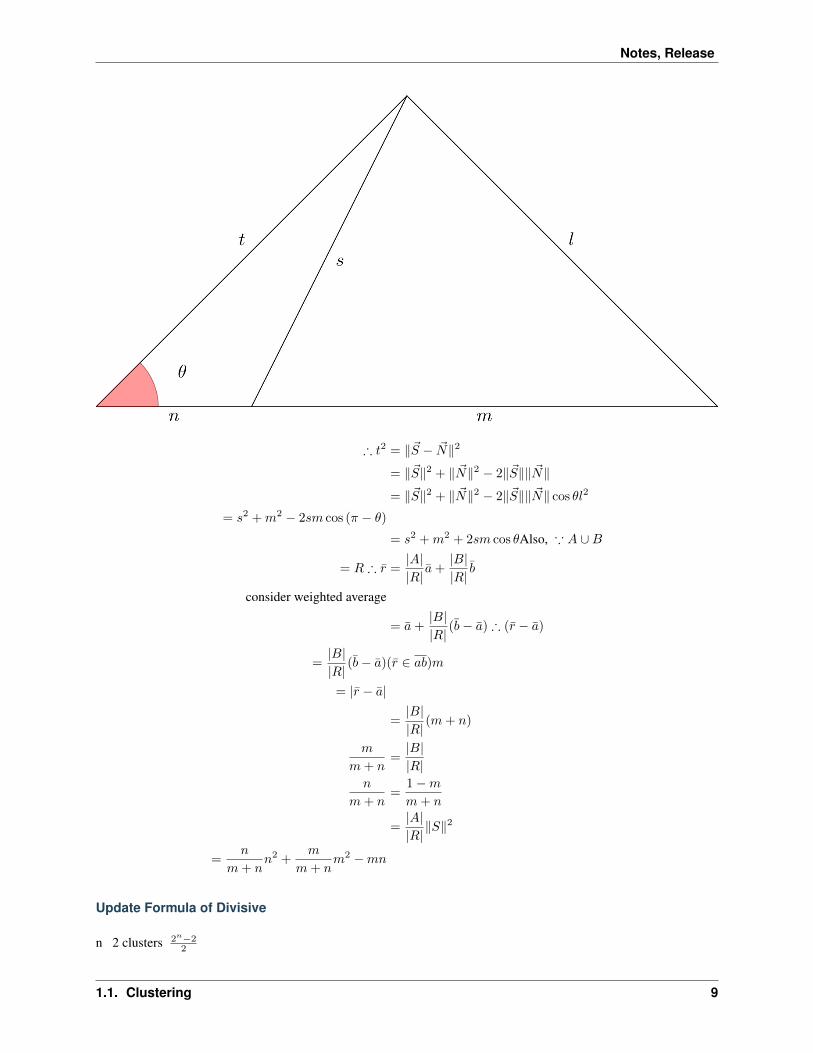
Fact 1: 1746, Steward proof that

𝑛

𝑚+ 𝑛𝑙2 +

𝑚

𝑚+ 𝑛𝑡2 = 𝑠2 +𝑚𝑛

Proof that 𝑇 = −


Notes, Release

∴ 𝑡2 = ‖ − ‖2

= ‖‖2 + ‖‖2 − 2‖‖‖‖

= ‖‖2 + ‖‖2 − 2‖‖‖‖ cos 𝜃𝑙2

= 𝑠2 +𝑚2 − 2𝑠𝑚 cos (𝜋 − 𝜃)= 𝑠2 +𝑚2 + 2𝑠𝑚 cos 𝜃Also, ∵ 𝐴 ∪𝐵

= 𝑅 ∴ 𝑟 =|𝐴||𝑅|

+|𝐵||𝑅|

consider weighted average

= +|𝐵||𝑅|

(− ) ∴ (𝑟 − )

=|𝐵||𝑅|

(− )(𝑟 ∈ 𝑎𝑏)𝑚

= |𝑟 − |

=|𝐵||𝑅|

(𝑚+ 𝑛)

𝑚

𝑚+ 𝑛=|𝐵||𝑅|

𝑛

𝑚+ 𝑛=

1−𝑚𝑚+ 𝑛

=|𝐴||𝑅|‖𝑆‖2

=𝑛

𝑚+ 𝑛𝑛2 +

𝑚

𝑚+ 𝑛𝑚2 −𝑚𝑛

Update Formula of Divisive

n 2 clusters 2𝑛−22

1.1. Clustering 9

Notes, Release

Agglomerative merge

proof:

x1 x2 x3 ... xnA B B ... A

Consider we encode vector as a binary string.

2𝑛 − 2 ( A or B)

binary complement e.g. AABAA v.s. BBABB

∴ 2𝑛−22

Divisive by Splinter Party

:

Init, cal Distance Matrix

𝑎 𝑏 𝑐 𝑑 𝑒𝑎 0 2 6 10 9𝑏 2 0 5 9 8𝑐 6 5 0 4 5𝑑 10 9 4 0 3𝑒 9 8 5 3 0

• a 6.75

• b

• c

• d

• e

∴ a

𝑎 vs 𝑏, 𝑐, 𝑑, 𝑒

step 2, old cluster

distance to old distance to new 𝛿b (5, 9, 8) = 7.33 2 5.33c 6d 10e 9

∀𝛿 > 0, 𝛿𝑚𝑎𝑥 = 𝑏

∴ 𝑏 leave

∴

𝑎, 𝑏 vs 𝑐, 𝑑, 𝑒

step 3 𝑐, 𝑒, 𝑑 goto step2


Notes, Release

∀𝛿 < 0, then stop.reslut: 𝑎, 𝑏 vs 𝑐, 𝑑, 𝑒

rule diameter

𝐷𝑖𝑚𝑡(𝑎, 𝑏) = 𝑚𝑎𝑥(2) = 2 (1.1)𝐷𝑖𝑚𝑡(𝑐, 𝑑, 𝑒) = 𝑚𝑎𝑥(4, 5, 3) = 5− > split 𝑐, 𝑑, 𝑒(1.2)

diameter < args => Stop or diameter change rate too high => stop

Agglomerative update formula

Distance Matrix

step1 x1, x2 x3 .. xn

x1 x2 x3 x4 x5

x1 x2

Divisive or Agglomerative Distance Matrix : Ω𝑛2

Experiment Suggestion

Hierarchical Method will much slower, if n grows up.

• If # of clusters less, starts from Divisive

• If # of clusters large starts from Agglomerative

1.1.3 Peak-Climbing Method

(Mode-Seeking Method)

User (blocks) . e.g.: 2-dimension -> Q x Q blocks

Valley-Seeking

e.g.: We have data point with 2-dimension, and 𝑄×𝑄 = 6𝑥× 6.

Then, counting the data point located in each blocks.

Table for example:

6 42 11 2 1 037 250 58 10 24 934 200 52 48 120 383 25 19 125 230 972 3 15 122 220 1120 5 7 52 190 46

∀ blocks, it has 8 neighbor. Find the max of neighbor.

if max(neighbor) > self, then neighbor

neighbor local max (cluster center)

p.s. cluster Peak

blocks number => 1 => local max

high-dimension e.g.: 5-dimension 35 − 1 = 243 neighbor

1.1. Clustering 11

Notes, Release

1.1.4 Graph-Theoretical Method

Tree: vertix neighbor loop

Definition Inconsistent Edge overlineAB

overlineAB A B Edge

Inconsistent Edge A B clusters

Neighborhood 2

Average_A = Neighborhood/ # of Neighborhood V_A = A

e.g AB - Average_A / Var_A ~= 22

Edge normail distribution 1% Edge z >= 3

Inconsistent

• AB Inconsistent

• Neighborhood

• threshold

– AB - Average_A | >= threshold

– AB | / Average_A

Minimal Spanning Tree (MST)

Tree edge

vecx_1 .. vecx_n MST

1. (e.g. A) A A Tree T_1

2. forall k = 2, 3, 4... T_k from T_k-1 by add (one of the) shortest edge from a node not in T_k-1 such thatT_k is still connected.

Complexity: theata n^2

therefore

MST MST edge inconsistency = - | AB - Avg_A | / Var_A > threshold

AB - Abg_B | / Var_B > threshold

inconsistency inconsistency

therefore connected graph disconnected graph

1980 - Gabriel Graph - Relative Neighborhood Graph - D DT

MST touching data

Definition of Gabriel Graph

for x_1, ... x_n

x_i, x_j

Disk(x_1, x_j)


Notes, Release

overlinex_i x_j

x_i - x_j | ^2 < | x_i - x_k | ^2 + | x_j - x_k | ^2, forall k != i, j

ref: ‘https://en.wikipedia.org/wiki/Gabriel_graph‘_

Definition of Relative Graph

x_i x_j | overlinex_i x_j |

Lune Lune x_k, x_i x_j

overlinex_i x_j in Relative Graph <=> | x_i - x_j | < Max | x_i - x_k | , | x_j - x_k | , forall k != i, j

• Lune Disk

therefore Lune Disk

therefore overlinex_i x_j Relative Graph edge, Gabriel Graph Edge

therefore Edge_RNG C Edge_Gabriel

•

Delaunay Triamgles

\ x1 /\ /\ /

x2 | x3||

Voronoi Diagram

Delaunay

Def x_i x_j (cell_i and cell_j) (e.g. cell_i and cell_j neighbor), overlinex_i, x_j

DT edge >> Gabriel Graph # of edge >= RNG >= MST

Voronoi Diagram for data point vecx_1 ... e.g. vecx_1 vecx_2

Each data point (cell_i) forall vecy in cell_i, | vecy - vecx_i | <= | vecy - vecx_j | forall j = 1 dots n (j != i)

Clustering via Graph Method

( vecx_1 ... vecx_2 ) inconsistency inconsistent edge,

e.g.

data point:

1.1. Clustering 13

Notes, Release

(1, 1)(1, 2)(1, 3)(2, 1)(2, 2)(2, 3)(3, 1)(3, 2)(3, 3)

(4, 4)(4, 6)(4, 8)(6, 4)(6, 6)(6, 8)(8, 4)(8, 6)(8, 8)

• MST break overline(3, 3) (4, 4)

1.1.5 Fuzzy Clustering

Fuzzy clustering hard clustering (crispy clustering)

e.g. k-means, hierarchical, peak-climbing... hard clustering

Definition

Fuzzy clustering

e.g.

A point:

• 0.4

• 0.4

• 0.2

B point: - 0.3 - ...

data structure’s detail hard clustering information

Fuzzy K-means

AKA. Fuzzy C-means, F.C.M

1973 Bezdek paper

x_1, ..., x_n K

let v_j | j=1...k k cluster centroid

q > 1

u_ij i _j


Notes, Release

therefore u_i1 + ... + u_ik = 100%

min sum (u_ij)^q | vecx_i - vecv_j | ^2 , i=1...n, k=1...k

ps. tradictional K-means:

min sum i=1...N | vecx_i vecv_j | ^2 , vecv_j vecx_i cluster centroid

therefore K-means F.K.M : u_ij = 0 or 1

min ( partial ... / partial ... = 0)

Algo(F.K.M)

1. k , vecj , j=1...k

#. update membership coeffiecent u_ij = [ | vecx_i - vecv_j | ^-2 ] ^(1/q-1) / suml=1..k[ | vecx_i -vecl | ^-2] ^(1-/q-1)

•

• 1/(q-1) fuzzy

1. update centroid vecv_j^new = (sumi=1...n(u_ij)^q times vecx_j) / sumi=1..n(u_ij)^q

Max | u_ij - u_ij^last run | < threshold => stop

q > 1 will make F.K.M converge. q 1 Fuzzy

e.g. let q = 1 + 1/1000, therefore 1/(q-1) = 1000

Assume | x_i - v_1 | = 1/sqrt50 | x_i - v_2 | = 1/sqrt49 | x_i - v_3 | = 1/sqrt48

u_i1 = 50^1000 / (50^1000 + 49^1000 + 48^1000) = 99.99...% u_i2 = 49^1000 / ‘’ = 10^-9 u_i3 = 48^1000 / ‘’ =10^-18

therefore x_i v_1 v_2 v_3 winner takes all

1973 Bezdek q = 2

Note: Fuzzy K-means local min

1.1.6 Monothetic Clustering

v.s. Ploythetic Clusttering Clustering poly,

e.g k-means, MST, Hierarchical

Monothetic

e.g.

Q1. Q2. ...

binary string 2^50 ~= 10^15 = 14

True False e.g. <= 15000 m

(e.g. ) Ans 1 e.g. cm / m

Ans 1 e.g. < 100 cm & >= 100 cm

1.1. Clustering 15

Notes, Release

Topic: for

Max Association Sum

Def Association Measure between variable x and y M(x, y) = | ( (1, 1) times (0, 0) ) - ( .. (1, 0) - (0, 1) .. ) |

e.g. table on e3

M(x, y) = | 2 times 2 - 2 times 2 | = 0 , low association

M(r, s) = | 4 times 2 - 2 times 0 | = 8, high association

Ans : e.g. | 6 times 1 - 1 times 1 | = 5 e.g. | (n/2) times (n/2) - 0 times 0 | = n^2 / 4

: 1. M_ij forall i,j

2. Sum_x = sumtheta != xM_xtheta = M_xy + Mxz + ... Sum_y = sumM_ytheta

3. Max Association Sum

e.g. y = v_2 , Sum_y

8 v_2 = 1 v_2 = 0

Then v1, v3, v4, v5, v6 table, Max Sum (a new iteration)

1.1.7 Analytical Clustering

Moment-Preserving

3-dim: google scholar Ja-Chen Lin, Real-time and automatic two-class clustering by analytical formulas

k clusters => p_1, p_2, ... p_k & x_1 x_2 ... x_k because 2k , therefore 2k

p_1 + p_2 + ... + p_k = 100% p_1 x_1 + p_2 x_2 + ... + p_k x_k = overlinex p_1 x_1^2k -1 + ... + p_x x_k^2k- 1 = overlinex^2k - 1

ps. k > 4 (by Galoi’s ), computer approximation

2-dim IEEE PAMI

Principal Axis(PA) of vecx_i_1 ^3000

Definition PA of (x_i, y_i)_i (overlinex, overliney)

2-dim vecx_A vecx_B vecx_A .. 3000 x p_A vecx_B .. 3000 x p_B PA vecx_A vecx_B PA

because p_A theta_a + p_B theta_B = overlinetheta therefore p_A theta_A + p_B (theta_A = pi) = overlinetheta

because p_B pi = overlinetheta - (p_a + p_b) theta_A p_A

proof

P_A X_A + P_B X_B = barX = 0

therefore P_A X_A = - P_B x_B also bary = 0

P_A Y_A = - P_B Y_B

P_A^2 X_A^2 = P_B^2 X_B^2 .. (1) P_A^2 Y_A^2 = P_B^2 Y_B^2 .. (2)

(1) + (2) = P_A^2(X_A^2 + Y_A^2) = P_B^2(Y_A^2 + Y_B^2) P_A^2 r_A^2 = P_B^2 r_B^2

P_A r_A = P_B r_B

P_A r_A + P_B r_B = barr

2 P_A r_A = 2 P_B r_B = barr


Notes, Release

r_B = 0.5 barr / P_B

r_A = 0.5 barr / P_A

k-means when k=2 initial

1. Fast, without iterations

2. No initial

3. Automatic

How to setup Equetions

1-dim: no need to memory answer 2-dim: need 3-dim: the only one using r

1.1.8 Vector Quantization

If we want to transfer 10000 vector data

𝑥1, 𝑥2, . . . , 𝑥10000

∀ is high-dimension (e.g. 16-dim).

Problem

How to speed up the data transfer? If we can accept error; we can accept losely transfer.

Solution

We can use VQ for data compression.

First, we can cluster vectors into 8 clusters. Then we get 8 centroid.

Thus, we only need to transfer 𝑐𝑒𝑛𝑡𝑟𝑜𝑖𝑑0, . . . , 𝑐𝑒𝑛𝑡𝑟𝑜𝑖𝑑7 and 10,000 numbers which represent the cluster belongsto.

And, ∀ 10,000 numbers, it only 3 bits to transfer (000 - 111).

Results

This method will get high transfer speed, but the error is quite larger.

Note: This 8 cluster centroids are so-called codebook. Each centroid is a codeword (codevector).

Codebook Generation

The commonly used Linde-Buzo-Gray (LBG) algorithm to create codebook.

In fact, it is k-means.

1.1. Clustering 17

Notes, Release

Conclusion

• If centroid come from known public data, then your vector data called Outside Data.(Data may irrelavent tocentroid)

• If codebook is generated from data, we call them Inside Data. Then, the error will be lower, but the transfer costraises.

e.g.: Assume we use our own codebook

• Data –> clustering –> 8 clusters

• Data –> classification –> more near to which cluster

Side-Matched VQ (SMVQ)

Goal To provide better visual image quality than original VQ.

• Porposed by Kim in 1992

Seed Block

5124 = 128 4× 4 blocks 128 + 128 - 1 = 255 blocks seed blocks

seed block VQ codeword seed blocks

Example

(512 x 512) 2-by-2 codebook 256 codewords (8bit for index)

codewords:

0. 0 0 0 0

1. 1 1 1 1

. . .

255. 255 255 255 255

Compression algorithm:

step 1. seed blocks, VQ index file (in-place)

step 2. 250 x 250 blocks

-4 44 4

+ - -3 3 | x y3 3 | z w

find

|𝑥− 4|+ |𝑦 − 4|+ |𝑥− 3|+ |𝑧 − 3|()codewords33443344


Notes, Release

original photo codeword

Disscusion

• “classical blocks” more => the quality of image raise

1.1.9 K-Modes

Category Data (Non-numerical )

1998, K-Modes

Mode

e.g. n = 5 , vecx_1 ... vecx_5 k = 2 given x_1 = (alpha, big) = x_4

x_3 = x_5 (beta, mid) x_2 = (beta, small)

Init

z_A = x_1 = (alpha, big) z_B = x_2 = (beta, small)

Iteration 1

1. x_3 to B cluster (because z_A z_B ) x_4 to A; x_5 to B

2. update centroid z_A = Mode x_1 = (alpha, big) = x_4 = (alpha, big) z_B = Mode (beta, small), (beta,mid), (meta, mid) = (beta, mid)

Iteration 2

1. A = x_1, x_4, B = x_2, x_3, x_5

2. update centroid z_A = (alpha, big) z_B = (beta, small) Stop!

ps.

A =

x_1 = (1, 1, ) x_2 = (1, 1, ) x_3 = (1, 1, )

B =

x_4 = (1, 1, ) x_5 = (2, 1, ) x_6 = (1, 2, )

Mode z_A (1, 1, ), Mode z_B = (1, 1, )

x_7 = (1, 1, )

2007, IEEE-T-PAMI “On the impact of Dissimilarity Measure”

e.g. for A

dots | dim 1 | dim 2 | dim 3 |1 | 3 | 3 | 1 |

| | | 1 || | | 1 || | | 0 || | | 0 |

1.1. Clustering 19

Notes, Release

for B

1 | 2 | 2 |2 | 1 | 1 |

diff measurement for (x_7, z_A) = (1 - (3 ) / 3) + (1- 3/3) + 1 = 1

(x_7, z_A) = (1- 2/3) + (1 - 2/3) + 1 = 1.6666

therefore x_7 A

Example

47 soybean data ( ) 35-dim 21-dim ( 14-dim )

4 - D_1: 10 point - D_2: 10 - D_3: 10 - D_4: 17

100 initials

| k-mods | 2007 |Accurarcy | 82.6% | 91.32% |Precision | 88.1% | 95.0% |

ps. e.g A class 130 : 110 20

B class 150 120 30

Accurarcy = frac110 + 120130 + 150

Precision_A = A , A

= frac110110 + 30 (: A )

Precision_B = frac120120 + 20

Recall Rate_A = frac110130

Better Initials for K-mods

Pattern Reconition Leter, vol 23 2002

: n point k clusters

let J = fracnk * 0.1 ~ 0.5

data random sub-sample J subset of data

abbr. CM = Cluster Modes abbr. FM = Finer Modes (Better Modes)

Input: k, J, data Output: k Modes

Step 1: sub-sampling. Initially set CMU = Then, for i = 1...j do (A) and (B)

1. for subset S_i of Data, randomly S_i modes, k-modes

Let CM_i k modes

2. CMU CM_i Union


Notes, Release

Step 2: Refinement For i = 1 ... J do CM_i CMU k clusters, FM_i

Step 3: Selection FM_i CMU i.e (Total Distortion )

Then, output best FM_i

Experiment

Accurarcy | Better initail method | Random initial |98% | 14 | 5 |94% | | 2 |89% | | 2 |77% | | 3 |70% | 5 | 0 |

68% | 0 sampling | 5 |66% | 1 | 3 |

ROCK Method

1.1.10 Fast Methods to Find Nearest Cluster Centers

e.g. k-means or VQ

Definition 𝑘 = # of clusters = codebook size codebook = 𝑦1, . . . , 𝑦𝑛

Definition = (𝑥1, ..., 𝑥16) 16

Goal .. math:

min \| \vecy_i - \vecx \| ^2=min [ \sum_j = 1^16 (y_ij - x_j)^2 ],i = 1, 2, .\dots, 128

centroid e.g. 𝑦1𝑦2

𝑑2(𝑐𝑢𝑟𝑟𝑒𝑛𝑡)𝑚𝑖𝑛 = ‖− 𝑦𝑐𝑢𝑟𝑟𝑒𝑛𝑡𝑚𝑖𝑛 ‖2 = 𝑚𝑖𝑛‖− 𝑦𝑙‖2, 𝑦𝑙 ∈

𝑦𝑖 ‖𝑦𝑖 − ‖2 ?

Partial Distance Elimination

1985 PDE Method

𝐼𝑓(𝑦𝑖1 − 𝑥1)2 + (𝑦𝑖2 − 𝑥2)2 + (𝑦𝑖3 − 𝑥3)2 > 𝑑2(𝑐𝑢𝑟𝑟𝑒𝑛𝑡)𝑚𝑖𝑛

1.1. Clustering 21

Notes, Release

TIE Method

Pre-Processing: O(k^2) = 128x127/2 = C^n_2

Main:

‖𝑦𝑖 − 𝑦𝑐𝑢𝑟𝑟𝑒𝑛𝑡𝑚𝑖𝑛 ‖ >= 2𝑑𝑐𝑢𝑟𝑟𝑒𝑛𝑡𝑚𝑖𝑛

𝑦𝑖

Proof

_\vecx//

/\vecy^current_min\\\ \vecy_i

‖𝑦𝑖 − ‖ >= |‖𝑦𝑖 − 𝑦𝑐𝑢𝑟𝑟𝑒𝑛𝑡𝑚𝑖𝑛 ‖ − ‖ 𝑦𝑐𝑢𝑟𝑟𝑒𝑛𝑡𝑚𝑖𝑛 − ‖| = | >= 2𝑑𝑐𝑢𝑟𝑟𝑒𝑛𝑡𝑚𝑖𝑛 − 𝑑𝑐𝑢𝑟𝑚𝑖𝑛| >= (2− 1)𝑑𝑐𝑢𝑟𝑚𝑖𝑛 = ‖ 𝑦𝑐𝑢𝑟𝑚𝑖𝑛 − ‖

IEEE-T-Com

1994 Torres & Huguel

>= 0

𝐼𝑓‖‖2 + ‖𝑦𝑖‖2 − 2(𝑦𝑖)𝑚𝑎𝑥(

16∑1

𝑥𝑗) >= 𝑑2𝑐𝑢𝑟𝑚𝑖𝑛

𝑜𝑟

𝐼𝑓‖‖2 + ‖𝑦𝑖‖2 − 2()𝑚𝑎𝑥(

1∑6𝑗=1𝑦𝑖𝑗) >= ”

𝑤ℎ𝑒𝑟𝑒𝑋𝑚𝑎𝑥 = 𝑚𝑎𝑥𝑥1, 𝑥2, , 𝑥16 = ‖‖𝑖𝑛𝑓𝑖𝑛𝑖𝑡𝑤ℎ𝑒𝑟𝑒3𝑥128𝑧ℎ𝑖

vecy_i vecy^cur_min

Fast Kick-out by an Inequality

IEEE-T-C.S.V.T 2000 K.S. Wu

‖− 𝑦𝑖‖2 = (𝑥− 𝑦𝑖)(𝑥− 𝑦𝑖) = ‖𝑥‖2 + ‖𝑦𝑖‖2 − 2𝑥𝑖

𝑙𝑒𝑡𝑑2(𝑥, 𝑦𝑖) = ‖𝑥− 𝑦𝑖‖ − ‖𝑥‖2

Now

𝑑2(𝑥, 𝑦𝑖) = ‖𝑥− 𝑦𝑖‖2 − ‖𝑥‖2 = (𝑥− 𝑦𝑖)(𝑥− 𝑦𝑖)− ‖𝑥‖2 = ‖𝑦𝑖‖2 − 2𝑥𝑖 >= ‖𝑦𝑖‖2 − 2‖𝑥‖‖𝑦‖ = ‖𝑦𝑖‖(‖𝑦𝑖‖ − 2‖𝑥‖)

∴ 𝑖𝑓‖𝑦𝑖‖(‖𝑦𝑖‖ − 2‖𝑥‖) >= 𝑑2(𝑐𝑢𝑟𝑟𝑒𝑛𝑡)𝑚𝑖𝑛

𝑑2(𝑥, 𝑦𝑖) >= ‖𝑦𝑖‖(‖𝑦𝑖‖ − 2‖𝑥‖) >= 𝑑2(𝑐𝑢𝑟𝑟𝑒𝑛𝑡)𝑚𝑖𝑛 (𝑑𝑒𝑓𝑖𝑛𝑒𝑎𝑠‖𝑥− 𝑦𝑐𝑢𝑟𝑟𝑒𝑛𝑡𝑖 𝑚𝑖𝑛‖2 − ‖𝑥‖2)

∴ 𝑦𝑖𝑦𝑐𝑢𝑟𝑟𝑒𝑛𝑡𝑚𝑖𝑛 𝑥


Notes, Release

Implementation

sort vecy_1 ... vecy_128

|y_1| <= | y_2 | <= ... <= |y_128|

Goal x y_i

Step 1 2 |x|, y_init y^current_min

let telda d^2_min = telda d^2(x, y_init)

let remaining set R = y_init centroid

Step 2

1. if R is empty set, the y^current_min is the answer; R y_i

2. |y_i| (|y_i| - 2 |x|) >= telda d^2_min, case i.

|y_i| >= |x| y_l | l>=i, goto step 2a

case ii. <= <= , goto step 2a

3. telda d (x, y_i) R y_i, telda d^2 (x, y_i) >= telda d^2_min, goto 2a

4. Let d^2_min = telda d^2(x, y_i) Let y^current_min = y_i goto step 2a

Step 2b case i and ii

∵ ‖𝑦𝑙‖(‖𝑦𝑙‖ − 2‖𝑥‖) >= ‖𝑦𝑖‖(‖𝑦𝑖‖ − 2‖𝑥‖) >= 𝑑2𝑚𝑖𝑛

∵ 𝑓(𝑡) = 𝑡(𝑡− 2‖𝑥‖) = 𝑡2 − 2‖𝑥‖𝑡𝑡 = ‖𝑥‖

Conclusion

| | 1994 | 1995 | Inequality |

• 512x512 4-by-4 VQ

Codebook Size Full Search Inequality128 30 s 4.5 5.3 1.89256 73 8 14.37 4.15512 146 13.7 27.24 7.23

1.1.11 Eliminate Noise via Hierar. Agglom. Method

Hierar Agglom D_centroid Noise

Problem If a pixel whose Grey Level is 𝑥, 0 <= 𝑥 <= 255 and the Grey Levle of 8 neighbor pixels is:

22 23 24239 x 235238 237 236

1. 8 neighbor Hierar Agglom e.g. A = 22, 23, 24, barA = 23.0 B = 235, 236, 237, 238, barB = 237.0threshold merge

2. Then, if ‖𝑥−𝐴‖ = ‖𝑥− 23.0‖ < 𝑡ℎ𝑟𝑒𝑠ℎ𝑜𝑙𝑑𝑁𝑜𝑖𝑠𝑒, x A cluster therefore x B cluster

3. If | x - barA | > threshold_Noise and | x - barB > threshold_Noise, x therefore x is noise therefore x

1.1. Clustering 23

Notes, Release

()

therefore Score 22 is |A| = 3

23 is |A|+1 = 3 + 1 = 4 24 is |A| = 3

Score 235 is |B| + 1 = 5 + 1 236 is |B| = 5 237 is |B| + 1 = 6 238 is |B| = 5 239 is |B| + 1 = 5 + 1

therefore Score_A = 3 + 4 + 3 = 10 Score_B = 6 + 5 + 6 + 5 + 6 = 28 therefore x in B, i.e 237

: T_Hierar = 25, T_Noise = 36

RMS = | Original - New |

RMS = 11 < Mediam Filter RMS = 19 < K-Means Filter RMS = 21

1.1.12 Clustering Aggregation by Probability Accumenulation

Wang, Yang, Zhou P.R. 2009 Vol 42 page. 668-675

𝑥1 . . . 𝑥𝑛 for each is m-dimension

~ c^(1) ... c^(9) 9

Step 1: Component Matrix [A]^(P), P = 1 ... 9

A^(P)_ii = 1, forall i = 1 ... n

/- 0, if x_i x_j in C(P)

A^(P)_ij = - frac11 + ( x_i, x_j )^(1/m)

Step 2

barA = P association = frac19 sum^9_P=1 [A]^(P)

Step 3 Then, transform barA into distance matrix

d(x_i, x_j) = 1 - barA(x_i, x_j) = 1 - barA_ij

Step 4 Hierar Merge( D_min)

big jump of distance

Exp

x_1 ... x_9 1-dim (e.g. k-means, k=3, )

exp 1:

• A cluster x_1, x_2

• B cluster x_3, x_4

• C cluster x_5, x_6, x_7

exp 2:

• A cluster x_1, x_3

• B cluster x_2, x_4, x_5

• C cluster x_6, x_7


Notes, Release

7,7 association matrix barA

2𝐴 = (𝑒𝑥𝑝)

| x_1 x_2 | x_3 x_4 | x_5 x_6 x_7 |x_1 | 1/(1+2) | 1/(1+2)x_2 | | (exp2)

x_3 | | 1/3 |x_4 | |

x_5 | | | 1/(1+3) 1/(1+3)x_6 |x_7 |

1 - barA

1−𝐴 = ...

Step 4: Hierar Merge e.g. x_1, x_3, x_4 vs x_5 vsx_6, x_7

half rings | 400 + 100 point | 2D

Iris | 50 + 50 + 50 point | 4| 100 point (10 clusters) | 64-dim| 683 (2 clusters) | 9-dim

Wine | 178 (3 cluster) | 13-dimGlass | 214 (6) | 9

Pre-processing Normalize Data mean = 0, var = 1 3

exp: run 10 times or 50 times exps, forall Data set k-means, k 10~30 e.g. 100~638 point , avg 349 point, squrt(349)= 19)

IEEE-T-PAMI 2005 “Evidence Accumulation” (EA)

2002 CE

Error Rate pre-processing

| EA | CE | PA |

2 half rings | 0 | 25.42 | 0 |3 rings | 0.8% | 49 | 0 |

1.1. Clustering 25

Notes, Release

| 5.7% | 24 | 8.6 |Iris | 33 | 33 | 33 |

| 65 || 30 |

average | 34 |

Conclusion

Pre-Processing data:

P.A 10% error rate

PA(2009) EA(2005)

• pre-proc, 3%

• pre-proc, 2%

PA CE(2002)

• pre-proc, 12%

• pre-proc, 19%

1.2 Cryptography

1.2.1 Chapter 2: Symmetric Cipher

A.k.a

• conventional encryption

• single key encryption

plaintext plaintext ciphertext encryption decryption

cryptanalysis encryption / decryption Area of “breaking the code”.

cryptology cryptography + cryptanalysis

Symmetric Cipher Model

1. Plaintext

2. Encryption Algorithm

3. Secret key: encryption algorithm input

4. Ciphertext: algo output

5. Decryption Algorithm

1. Encryption algorithm ciphertext decryption secret key plaintext ciphertext secret key

2. Sender receiver share secret key


Notes, Release

secret key algorithm algorithm

Cryptography

1. Operations substitution reversible substitution product systems

2. Key shared key symmetric sender / receiver key asymmetric

3. Plaintext

• block cipher

• stream cipher

Cryptanalysis attack

• Ciphertext only

• Known plaintext

– plaintext-ciphertext pair(s)

• Chosen plaintext

• Chosen ciphertext

• Chose Text

• unconditional secure

–

• computational secure

– cost plaintext

– computation

* DES: 56 bits

* triple DES: 168 bits

* AES: 128 bits

Substitution Techniques

Substitution and transposition

Caesar Cipher

𝐸(𝑘, 𝑝) = (𝑝+ 𝑘) mod 26

𝐷(𝑘, 𝑐) = (𝑝− 𝑐) mod 26

Key space 25

1.2. Cryptography 27

Notes, Release

Monoalphabetic Cipher

Caesar Cipher permutation key space 26!

cryptanalysis e.g. ciphertext frequency table ciphertext

Playfair Cipher

Multiletter cipher

Hill Cipher

Multiletter cipher

= 𝑝𝐾𝑚𝑜𝑑26𝑝 = 𝐾−1𝑚𝑜𝑑26

Vigenere Cipher

Let 𝑘𝑖 key 𝑗 (shift j) Caesar Cipher

𝑐𝑖 = (𝑝𝑖 + 𝑘𝑖𝑚𝑜𝑑𝑚)𝑚𝑜𝑑26𝑝𝑖 = (𝑐𝑖 − 𝑘𝑖𝑚𝑜𝑑𝑚)𝑚𝑜𝑑26

key repeat plaintext

E.g.:

key = hellohellohemsg = magic numberc = ...

julia> caesar(k, p) = Char((Int(p) - Int('a') + Int(k) - Int('a')) % 26 + Int('a'))caesar (generic function with 1 method)

julia> map(x->caesar(x...), zip(key, msg))12-element ArrayChar,1:'t''e''r''t''q''[''r''f''x''p''l''v'

Vernam Cipher

binary data cryptanalysis frequency table

𝑐𝑖 = 𝑝𝑖𝑘𝑖𝑝𝑖 = 𝑐𝑖𝑘𝑖

(xor)


Notes, Release

One-Time Pad

Improve Vernam Cipher.

Random key plaintext repeat

key message cryptanalysis

perfect secrecy

Transposition Techniques

permutation

Rail Fence

msg: meet me after the party

m e m a t r h p r ye t e f e t e a t

transposition cipher frequency plaintext frequency Digram/Trigram table

Rotor Machine

1.2.2 Chapter 4: Number Theory

Groups

𝐺, ·set binary operation Group

Rings

𝑅,+,×set addition operator multiplication operation

Fields

𝐹,+,×set addition operator multiplication operation axioms

Note: integer set field multiplication inverse

3 13

13 integer set

E.g.

•

•


Notes, Release

Finite Fields

cryptography finite field finite field order length(F) 𝑝𝑛, where 𝑝 is a prime, 𝑛 ∈ N.

Galois Field

𝐺𝐹 (𝑝𝑛)

The set with modulo arithmetic operations denote as 𝐺𝐹 (𝑝) = 𝑍𝑛 n prime element multiplication inverse elementn

𝑍𝑝

𝑎, 𝑏𝑏 multiplication inverse extended Euclidean algorithm

𝑎𝑥+ 𝑏𝑦 = 1 = 𝑔𝑐𝑑(𝑎, 𝑏)

[(𝑎𝑥 mod 𝑎) + (𝑏𝑦 mod 𝑎)] mod 𝑎 = 1 mod 𝑎

[0 + (𝑏𝑦 mod 𝑎)] mod 𝑎 = 1

𝑏𝑦 mod 𝑎 = 1

∴ 𝑦 = 𝑏−1 is multiplication inverse of 𝑏.

Polynomial Arithmetic

Ordinary Polynomial Arithmetic

•

• Field N

Finite Fields of 𝐺𝐹 (2𝑛)

8 bits data8 bits 0~255 𝐺𝐹 (28) order 251 8 bits Field 251~255

𝑓(𝑥)𝑚𝑜𝑑𝑚(𝑥) = 𝑚(𝑥)− 𝑓(𝑥)

Generator

generator

(mod order-1)

𝐺(2𝑛) with irreducible polynomial 𝑓(𝑥)

Let 𝑓(𝑥) = 0 generator 𝑔

1.2.3 Chapter 8: More about Number Theory

Fermat’s and Euler’s Theorems

Fermat’s Theorem

𝑝 𝑝 𝑎


Notes, Release

𝑎𝑝−1 mod 𝑝 = 1 ( 1

𝑎𝑝 mod 𝑝 = 𝑎 mod 𝑝

Euler’s Totient Function

𝜑(𝑛)

n n

𝜑(8) = 4

𝜑(37) = 36

𝑝, 𝑞

𝜑(𝑝𝑞) = 𝜑(𝑝)× 𝜑(𝑞) = (𝑝− 1)(𝑞 − 1)

𝜑(21) = 𝜑(3× 7) = 𝜑(3)× 𝜑(7) = (3− 1)(7− 1) = 12

Euler’s Theorem

𝑎, 𝑛

𝑎𝜑(𝑛) ≡ 1( mod 𝑛)

𝑎𝜑(𝑛) mod 𝑛 = 1

alternative form

𝑎𝜑(𝑛)+1 ≡ 𝑎( mod 𝑛)

Testing for Primality

Miller-Rabin Algorithm

property of prime

First property: 𝑝 is a prime, 𝑛 < 𝑝, 𝑛 ∈ N

(𝑎 mod 𝑝)× (𝑎 mod 𝑝) = (𝑎2 mod 𝑝)

Given

𝑎 mod 𝑝 = 1

(or)𝑎 mod 𝑝 = −1

iff

𝑎2 mod 𝑝 = 1


Notes, Release

Discrete Logarithm

Primitive Root

𝑎, 𝑝

𝑎 𝑎𝜑(𝑝)=𝑝−1 ≡ 1( mod 𝑝) 1

𝑎1, 𝑎2, . . . , 𝑎𝑝−1 mod output

primitive root

𝑎 𝑝 primitive root

integer primitive root

Logarithm for Modular Arithmetic

𝑝 primitive root 𝑎

𝑏

𝑏 ≡ 𝑎𝑖( mod 𝑝)

𝑎 primitive root 𝑎𝑖 1, ,𝑝− 1

1.2.4 Hash Functions

Hash function 𝐻 input data 𝑀 output

ℎ = 𝐻(𝑀)

data integrity checksum

Cryptography Hash Functions

• One-way property: computational infeasible to find the data object, given a certain hash. hash hash

• Collision-free property: input data pair hash value

hash functions data integrity

Application of Cryptography Hash Functions

Message Authentication

Alice Bob data Hash values data’ Bob Hash values data integrity

man-in-the-middle-attack

Darth append hash value Bob

Figure 11.3

1. data encryption

2. hash value


Notes, Release

3. data hash value shared key

4. double protection.

Message Authentication Code

A.k.a keyed hash function

shared secret key authentication

Practices: SSL/TLS

𝐸(𝐾,𝐻(𝑀))

• MAC shared secret key

• Chap 12

Digital Signature

1. message sensitive M digital signature Alice sign

2. message sign

Other Hash Functions Uses

• Password saved in DataBases. (One-way password file)

• intrusion detection

• virus detection

• pseudorandom function (PRF) or a pseudorandom number generator (PRNG)

Two Simple Hash Functions

input iteration

insecure

1. n block block bit-by-bit XOR

2. block + circular shift block shift 1 shift 2

Hash functions block collision hash functions XOR

Requirements and Security

Preimage

𝑥 is the preimage of ℎ for a hash values

Collision

If 𝑥 = 𝑦, but 𝐻(𝑥) = 𝐻(𝑦)

Requirements (table 11.1)


Notes, Release

• input

• output

• Efficiency: forward pass

• preimage resistant: one-way.

• Second preimage resistant: weak collision resistant. Given 𝑥 collision (computational infeasible)

• Strong collision resistant: ∀(𝑥, 𝑦) pair, no collision. (computational infeasible)

• Pseudorandomness: hash value pseudorandomness

Attacks

1. Brute-Force

2. Cryptanalysis: attack the algorithm property.

Brute-Force Attacks

m-bit hash value,

hash value ℎ preimage (input) random input input hash value 2𝑚

2𝑚−1

second preimage? 𝑥 ℎ 𝑦, 𝑠.𝑡.𝐻(𝑦) = 𝐻(𝑥) 2𝑚

Collision Resistant: 2𝑚/2 ?

MD4/MD5 -> 128 bit

Cryptanalysis

•

Hash Functions Based on Cipher Block Chaining

11.8 MD4/MD5/SHA-family

SHA

SHA-512

Message block padding

chain result

1.3 DL

1.3.1 Part I

Math basic


Notes, Release

Machine Learning

Problem setting:

1. meta-rule meta-rule e.g. meta-rule meta-rule

2. 𝑥 𝑦 learning optimization

e.g. DNS and cancer

Linear Model

• XOR linear model feature extraction NN

Linear Regression

Multivariate Linear Regression:

ℎ𝜃() = 𝜃𝑇

• MSE cost function

𝐽(𝜃) =1

2𝑚

𝑚∑𝑖

(ℎ𝜃()− 𝑦)2

cost function 𝑋 = 𝑥1, . . . , 𝑥𝑚 data set 𝑋 𝐽(𝜃) data set 𝐽(𝜃) 𝜃

• cost function close form solution, Normal Equation Method GD why ?

– http://stats.stackexchange.com/questions/23128

– inverse matrix 𝑂(𝑛3)

Univariable Linear Regression

• Univariable ->

Assume:

ℎ𝜃0,𝜃1(𝑥) = 𝜃0 + 𝜃1𝑥

The cost function will be:

𝐽(𝜃0, 𝜃1) =1

2𝑚

𝑚∑𝑖

(ℎ𝜃0,𝜃1(𝑥𝑖)− 𝑦𝑖)2

Then, if we simplify ℎ, let 𝜃0 = 0,

𝐽(𝜃1) =1

2𝑚

𝑚∑𝑖

(ℎ𝜃1(𝑥𝑖)− 𝑦𝑖)2 (1.3)

=1

2𝑚

𝑚∑𝑖

(𝜃1𝑥𝑖 − 𝑦𝑖)2(1.4)

Objective function:

𝑎𝑟𝑔min𝜃1

𝐽(𝜃1)

1.3. DL 35

http://stats.stackexchange.com/questions/23128

Notes, Release

It looks like this:

This objective function is convex and has a close form solution.

Polynomial Regression

Change linear to higher-order ploynomial model

e.g.

ℎ(𝑥) = 𝜃0 + 𝜃1𝑥1 + 𝜃2𝑥2 + 𝜃3𝑥21 + 𝜃4𝑥

22

Gradian Descent

• learning rate 𝜂 linear regression

– minimum 𝜂 iteration minimum cost function iteration

• Batch Gradian Descent, training set

• http://mccormickml.com/2014/03/04/gradient-descent-derivation/

Logistic Regression

classifcation algo.

outcome

0 ≤ ℎ(𝑥) ≤ 1


http://mccormickml.com/2014/03/04/gradient-descent-derivation/

Notes, Release

Sigmoid function (logistic function):

𝜎(𝑧) =1

1 + 𝑒−𝑧

Model

ℎ𝜃() = 𝜎(𝜃𝑇 ) (1.5)

=1

1 + 𝑒−𝜃𝑇 (1.6)

Logistic Regression with MSE

If we select MSE as cost function, we will obtain non-convex cost function.

1.3. DL 37

Notes, Release

< 0 local optima > 0 global optima

MSE Logistic Regression

Logistic Regression Cost Function

𝐽(𝜃) =1

𝑚

𝑚∑𝑖

𝐶𝑜𝑠𝑡(ℎ𝜃(𝑥𝑖), 𝑦𝑖)

𝐶𝑜𝑠𝑡(ℎ𝜃(𝑥), 𝑦) =

− log(ℎ𝜃(𝑥)), if 𝑦 = 1

− log(1− ℎ𝜃(𝑥)), if 𝑦 = 0(1.7)

= −𝑦 log(ℎ𝜃(𝑥))− (1− 𝑦) log(1− ℎ𝜃(𝑥))(1.8)

In case of 𝑦 = 1


Notes, Release

ℎ𝜃(𝑥) , ℎ𝜃(𝑥) (0, 1) Domain (0, 1) 0 1 log convex function

In case of 𝑦 = 0

1.3. DL 39

Notes, Release

Differentiation Linear Regression with MSE why?

Normal Equation Method

𝜃 = (𝑋𝑇𝑋)−1𝑋𝑇

Julia code:

pinv(X' * X) * X' * y

Example

(x, y) = (1, 2), (2, 4), (3, 6)

𝑦 = 2𝑥

julia> X = A[:, 1:2]3×2 ArrayInt64,2:1 12 13 1

julia> Y = A[:, 3]3-element ArrayInt64,1:246


Notes, Release

julia> pinv(X' * X) * X' * Y2-element ArrayFloat64,1:2.0-1.02141e-14

or

julia> X \ Y2-element ArrayFloat64,1:2.02.88619e-15

If Non-interible

• pinv vs inv

– pinv – psudo-inverse

causes:

• Redundant feature – linear dependent (?)

– e.g. 𝑥1 = 3𝑥2

– GD cost function 𝐽

• Too many feature

– training data

– linear regression feature 𝜃 parameter Regularization

ReLU

relu(x) = (x > 0) ? x : 0

https://en.wikipedia.org/wiki/Rectifier_(neural_networks)

• low computational cost.

• deep MLP back propagation sigmoid function or tanh layer sigmoid tanh upper / lower bound deepMLP

• ReLU x 0 topology fully connected NN outcome 0 connection

Feature Scaling

Linear Regression: Linear Regression MSE GD feature scale cost function GD Rescaling cost function GD

Mean Normalization

𝑥′ =𝑥− 𝜇

𝑥𝑚𝑎𝑥 − 𝑥𝑚𝑖𝑛

1.3. DL 41

https://en.wikipedia.org/wiki/Rectifier_(neural_networks

Notes, Release

standard deviation

𝑥′ =𝑥− 𝜇𝜎

model 𝜎, 𝜇

Data

• face detection

– learning

– learn

– learning

– financial data

Learning Rate Selection

Learning rate 𝜂 hyper parameter algo linear regression fixed learning rate GD 𝜂 cost function iteration/epochplotting learning rate

1.3.2 Regularization

• 𝐿0, 𝐿1, 𝐿2 regularization: penalty term loss function

• Data Augmented: data noise model robustness

• Share Weight

• Bigging, boosting

• DropOut: for NN http://cs.nyu.edu/~wanli/dropc/

Single Hidden Layer MLP

Input tuple hidden layer node sample input domain -> label domain space dictionary table table overfitting

(w) generalization

Data Augmented

• Image deformation: noise

– Deep Big Simple Neural Nets Excel on Hand-written Digit Recognition

Share Weight

parameter (or weight in NN context) overfitting CNN


http://cs.nyu.edu/~wanli/dropc/

Notes, Release

1.3.3 Autoencoder

Feature extraction: feature representation

Let 𝜑 is encoder.

Let 𝜓 is decoder.

𝜑 = 𝑋 → 𝐹

𝜓 = 𝐹 → 𝑋

Objective function:

𝑎𝑟𝑔min𝜑,𝜓‖𝑋 − 𝜓(𝜑(𝑋))‖2

Undercomplete Autoencoder hidden coding . non-linear undercomplete autoencoder overfittinggenerization

Overcomplete Autoencoder coding

1.4 Evolutionary Neuron Network

1.4.1 Formulating Problem

Elements

• Mapping genotype encoding with a mapping phenotype.

• Fitness function

Representation

• Tree Encoded

• Graph Encoded

Common Algo

There ar four common evolutionary computation (EC) algorithms.

• Genetic Algorithms

• Genetic Programming

• Evolutionary Strategies

• Evolutionary Algorithms

Genetic Algorithms

• string encoding for genotype

1.4. Evolutionary Neuron Network 43

Notes, Release

Genetic Programming

A specialized type of GA without string encoding, but tree based coding for graph problem.

• different mutation operation, like swapping branch of tree.

• length of genotypes in GP can be variable.

Evolutionary Strategies

ES is another variation of simple GA approach. It evolves not only the genotypes but the evolutionary parameters, thestrategy itself.

Evolutionary Algorithms

A specialized algo for evolving the transition table of Finit State Machine.

1.5 Paper

1.5.1 Deep Big Simple Neural Nets Excel on Hand-written Digit Recognition

tag NN, MLP, GPU, training set deformations, MNIST, BP

ref https://arxiv.org/pdf/1003.0358.pdf

dataset MNIST

Data Preproc

Elastic deformation (Elastic distortion) regularization generization

Feature scaling [-1.0, 1.0]

Learning Algo

• On-line BP without momentum (what is momentum on BP?).

• 2 - 9 hidden layers MLP

• Arch descibe in table 1

• learning rate

1.5.2 Tiled convolutional neural networks

ref https://papers.nips.cc/paper/4136-tiled-convolutional-neural-networks.pdf

• “convolutional (tied) weights significantly reduces the number of parameters”


https://arxiv.org/pdf/1003.0358.pdf

https://papers.nips.cc/paper/4136-tiled-convolutional-neural-networks.pdf

Notes, Release

1.5.3 TODO

• https://arxiv.org/pdf/1103.4487.pdf

1.6 PRML

1.6.1 Introduction

• pattern recognition discover rules, regularities of data.

• Common symbol

– data point

– target vector

– result of ML algo ()

• generalization:

• feature extraction: data pre-processing.

• deal with over-fitting

– Regularization term

–

– Bayesian approach

Regularization

One of technique to control over-fitting. Simply add a penalty term to the error function.

𝐸() = square error + regularization

regularization =𝜆

2‖‖2

w_0, w_0

• L2 Norm

• shrinkage

• Neuro network weight decay

Probability Theorem

• random variable is a function, e.g X, output can be foo or bar.

• Two rules:

– sum rule: Total Probability

– product rule

𝑝(𝑋 = 𝑓𝑜𝑜)− > 0.4; 𝑝(𝑋 = 𝑏𝑎𝑟)− > 0.6.

𝑝(𝑓𝑜𝑜) + 𝑃 (𝑏𝑎𝑟) = 1.

1.6. PRML 45

https://arxiv.org/pdf/1103.4487.pdf

Notes, Release

Joint Probability

𝑋 𝑌

X a random var, possibile outcome is 𝑎, 𝑏, 𝑐

Y a random var, 𝑓𝑜𝑜, 𝑏𝑎𝑟, 𝑏𝑎𝑧

N total number of trails

𝑛𝑖𝑗 : the number of 𝑋𝑖 + # of 𝑌𝑗

joint probability

𝑝(𝑋 = 𝑥𝑖, 𝑌 = 𝑦𝑗) =𝑛𝑖𝑗𝑁

or

𝑃 (𝑋 ∩ 𝑌 )

e.g.

𝑝(𝑋 = 𝑥𝑎, 𝑌 = 𝑦𝑏𝑎𝑟) =𝑛𝑎−𝑏𝑎𝑟𝑁

a bar 𝑋 𝑌

marginal probability or says sum rule

𝑝(𝑋 = 𝑥𝑖) =∑𝑗

𝑝(𝑋 = 𝑥𝑖, 𝑌 = 𝑦𝑗)

Condition Probability

Given 𝑋 = 𝑥𝑖

𝑝(𝑌 = 𝑦𝑗 |𝑋 = 𝑥𝑖) =𝑛𝑖𝑗𝑛𝑖

Product Rule

𝑝(𝑋 = 𝑥𝑖, 𝑌 = 𝑦𝑗) = 𝑝(𝑌 = 𝑦𝑗 |𝑋 = 𝑥𝑖)𝑝(𝑋 = 𝑥𝑖)

= 𝑝(𝑋 = 𝑥𝑖|𝑌 = 𝑦𝑗)𝑝(𝑌 = 𝑦𝑗)

Bayes’ Theorem

joint probability

𝑝(𝑌 |𝑋) =𝑝(𝑋|𝑌 )𝑝(𝑌 )

𝑝(𝑋)

• const, normalization term 𝑝(𝑦𝑖|𝑋)

∵ 𝑝(𝑋,𝑌 ) = 𝑝(𝑌,𝑋)

𝑝(𝑌 |𝑋)𝑝(𝑋) = 𝑝(𝑋|𝑌 )𝑝(𝑌 )

∴ 𝑝(𝑌 |𝑋) =𝑝(𝑋|𝑌 )𝑝(𝑌 )

𝑝(𝑋)


Notes, Release

Example

𝑋&𝑌 𝑥𝑖 𝑋 𝑌

prior probability ( 𝑥𝑖 ) 𝑌

𝑝(𝑌 )

posterior probability 𝑥𝑖

𝑝(𝑌 |𝑥𝑖)

Likelihood

𝐿𝑖𝑘𝑒𝑙𝑖ℎ𝑜𝑜𝑑 = 𝑝(𝑥𝑖|𝑦𝑗)

𝑥𝑖 Likelihood function 𝑦𝑗 𝑥𝑖

e.g.

𝐿𝑖𝑘𝑒𝑙𝑖ℎ𝑜𝑜𝑑 = 𝑝(| = 10−8)− >

Probability Density

outcome 𝑝(𝑥 ∈ (𝑎, 𝑏))

𝑝(𝑥 ∈ (𝑎, 𝑏)) =

∫ 𝑏

𝑎

𝑝(𝑥)𝑑𝑥

Note: 𝑝(𝑥) probability mass function

Transformation of Probability Densities

𝑥 = 𝑔(𝑦) 𝑥 𝑦

𝑝𝑦(𝑦)𝑑𝑦 = 𝑝𝑥(𝑥)𝑑𝑥 (1.9)

𝑝𝑦(𝑦) = 𝑝𝑥(𝑥)𝑑𝑥

𝑑𝑦(1.10)

= 𝑝𝑥(𝑥)𝑔′(𝑦)(1.11)= 𝑝𝑥(𝑔(𝑦))𝑔′(𝑦)(1.12)

ref: https://www.cl.cam.ac.uk/teaching/2003/Probability/prob11.pdf

Cummulative Distribution Function

𝑝(𝑥) 𝑃 (𝑥) 𝑃 ′(𝑥) 𝑝(𝑥)

𝑃 (𝑧) =

∫ 𝑧

−∞𝑝(𝑥)𝑑𝑥

1.6. PRML 47

https://www.cl.cam.ac.uk/teaching/2003/Probability/prob11.pdf

Notes, Release

Multi-variable

= [𝑥1, 𝑥2, . . . , 𝑥𝐷] continueous variable

join probability density function:

𝑝() = 𝑝(𝑥1, . . . , 𝑥𝐷)

:

𝑝() ≥ 0∫𝑝()𝑑 = 1

Sum Rule and Product Rule:

𝑝(𝑥) =

∫𝑝(𝑥, 𝑦)𝑑𝑦 (1.13)

𝑝(𝑥, 𝑦) = 𝑝(𝑦|𝑥)𝑝(𝑥)(1.14)

measure theory

Expectation

function 𝑓(𝑥), 𝑓(𝑥) under 𝑝(𝑥)

discrete :

E[𝑓 ] =∑𝑥

𝑝(𝑥)𝑓(𝑥)

continueous :

E[𝑓 ] =

∫𝑝(𝑥)𝑓(𝑥)𝑑𝑥

continueous probability density function N 𝑝(𝑥) 𝑥 :

E[𝑓 ] ≃ 1

𝑁

𝑁∑𝑛=1

𝑓(𝑥𝑛)

multi-variable () 𝑥 y function:

E𝑥[𝑓(𝑥, 𝑦)]

Conditional Expectation

E[𝑓 |𝑦] =∑𝑥

𝑝(𝑥|𝑦)𝑓(𝑥)

Variance

variance of 𝑓(𝑥)

𝑣𝑎𝑟[𝑓 ] = E[(𝑓(𝑥)− E[𝑓(𝑥)])2]

𝑣𝑎𝑙𝑢𝑒−𝑚𝑒𝑎𝑛 mean


Notes, Release

Covariance

random variables 𝑥, 𝑦

𝑐𝑜𝑣[𝑥, 𝑦] = E𝑥,𝑦[𝑥𝑦]− E[𝑥]𝐸[𝑦]

Matrix version:

𝑐𝑜𝑣[𝑋,𝑌 ] = E𝑋,𝑌 [𝑋𝑌 𝑇 ]− E[𝑋]𝐸[𝑌 𝑇 ]

Bayesian Probability

Aka, Subjective Probability.

Bayesian probability e.g.

Curve fitting problem frequentist model parameter 𝑤 uncertainty

prior probability posterior probability

data point 𝒟 = 𝑡1, 𝑡2, . . . , 𝑡𝑛 curve fitting

posterior probability 𝒟

(Event) posterior probability

𝑝(|𝒟) =𝑝(𝒟|)𝑝()

𝑝(𝒟)

right-hand side 𝑝(𝒟|) likelihood function likelihood function hyperparameter 𝒟 probable

posterior ∝ likelihood× prior

function function 𝑝(𝒟) normalization constant 𝑝(|𝒟) sum 1 :∫𝑝(|𝒟)𝑑 =

∫𝑝(𝒟|)𝑝()

𝑝(𝒟)𝑑 (1.15)

⇒ 1 =

∫𝑝(𝒟|)𝑝()

𝑝(𝒟)𝑑 (1.16)

⇒ 1 =1

𝑝(𝒟)

∫𝑝(𝒟|)𝑝()𝑑 (1.17)

⇒ 𝑝(𝒟) =

∫𝑝(𝒟|)𝑝()𝑑 (1.18)

likelihood function 𝑝(𝒟) 𝑝() distribution (uncertainty) frequentist fixed parameter error

maximum likelihood frequentist likelihood function

• ref: https://stats.stackexchange.com/questions/74082/

• ref: https://stats.stackexchange.com/questions/180420/

data set error function outcome

error function likelihood function error function log

maximizing likelihood minimizing error function

1.6. PRML 49

https://stats.stackexchange.com/questions/74082/

https://stats.stackexchange.com/questions/180420/

Notes, Release

log ? 𝑝(𝒟|) D 𝑡1, . . . .𝑡𝑛

𝑝(𝐷|) =𝑝(𝐷 = 𝑡1)𝑝(𝐷 = 𝑡2) . . . 𝑝(𝐷 = 𝑡𝑛)

𝑝()

log log function monotonically decreasing function, imply convex, maximum likelihood

Bayesian prior likelihood overfitting 3 head maximum likelihood 𝑝(ℎ𝑒𝑎𝑑) = 1 overfitting Bayesian priormaximum likelihood

frequentist Bayesian Bayesian prior

hyperparameter

model, model parameter hyperparameter.

𝑝(|𝛼), where 𝛼 is the precision of the distribution.

predictive distribution maximum likelihood 𝑤𝑀𝐿 𝛽𝑀𝐿 probabilistic model 𝑥

𝑝(𝑡|𝑥, 𝑤𝑀𝐿, 𝛽𝑀𝐿) = 𝒩 (𝑡|𝑦(𝑥, 𝑤𝑀𝐿), 𝛽−1𝑀𝐿)

Data Sets Bootstrap

frequentist

Original data set 𝑋 = 𝑥1, . . . , 𝑥𝑁

New data set 𝑋𝐵 random sampling with replacement e.g.: 10 original data set 3 10 𝑋𝐵

Curve fitting Re-visited

curve fitting polynomial frequentist maximum likelihood model

Probabilistic perspective target value distribution uncertainty

𝑥 𝑡 gaussian distribution distribution 𝜇 = 𝑦(𝑥, )

curve fitting 𝑦(𝑥, ) , target distribution

distribution

𝑝(𝑡|𝑥, , 𝛽) = 𝒩 (𝑡|𝜇, 𝛽−1)

= 𝒩 (𝑡|𝑦(𝑥, ), 𝛽−1)

Where the precision 𝛽−1 = 𝜎2

training data , maximum likelihood , 𝛽 i.i.d likelihood function

𝑝(𝑡|, , 𝛽) =

𝑁∏𝑛

𝒩 (𝑡𝑛|𝑦(𝑥𝑛, ), 𝛽−1)

Gaussian Function log likelihood form

ln 𝑝(𝑡|, , 𝛽) = −𝛽2

∑(𝑦(𝑥𝑛, )− 𝑡𝑛

)2+𝑁

2ln𝛽 − 𝑁

2𝑙𝑛(2𝜋)


Notes, Release

maximum log likelihood with respect with 𝛽

max−1

2

∑(𝑦(𝑥𝑛, )− 𝑡𝑛

)2⇒

min1

2

𝑁∑𝑛

(𝑦(𝑥𝑛, )− 𝑡𝑛

)2sum-of-square error function sum-of-square error function Gaussian noise distribution maximum likelihood

precision

1

𝛽=

1

𝑁

𝑁∑𝑛

(𝑦(𝑥𝑛, 𝑤𝑀𝐿)− 𝑡𝑛

)2𝑤𝑀𝐿, 𝛽𝑀𝐿 𝑥 predictive distribution

𝑝(𝑡|𝑥, 𝑤𝑀𝐿, 𝛽𝑀𝐿) = 𝒩 (𝑡|𝑦(𝑥, 𝑤𝑀𝐿), 𝛽−1𝑀𝐿)

Bayes’ theorem priorrecall this

𝑝𝑜𝑠𝑡𝑒𝑟𝑖𝑜𝑟 ∝ 𝑙𝑖𝑘𝑒𝑙𝑖ℎ𝑜𝑜𝑑× 𝑝𝑟𝑖𝑜𝑟

model distribution D-dimension Gaussian

𝑝(|𝛼)𝑎 = 𝒩 (|0, 𝛼−1𝐼)

=( 𝛼

2𝜋

)𝑀+12

𝑒−𝛼2

𝑇

where 𝛼 is the precision (𝛼−1 = 𝜎2)

maximum posterior log posterior likelihood exp prior exp

𝛽

2

𝑁∑𝑛


)2+𝛼

2𝑇

=

1

2

𝑁∑𝑛


)2+

𝛼

2𝛽𝑇

=

1

2

𝑁∑𝑛


)2+𝜆

2𝑇

sum-of-square error function with regularization term, given 𝜆 = 𝛼𝛽

prior maximum posterior regularization term over-fitting problem Gaussian distribution

Bayesian curve fitting

prior distribution 𝑝(|𝛼) maximum posterior Bayesian Bayesian product rule and sum rules (marginalization)Bayesian method

1.6. PRML 51

Notes, Release

predictive distribution posterior

𝑝(𝑡|𝑥, , ) = 𝑝(𝑡|𝑥,𝒟) =

∫𝑝(𝑡|𝑥, )𝑝(|𝒟)𝑑

𝛼, 𝛽 hyperparameter 𝑝(|𝒟) posterior

posterior Gaussian predictive distribution Gaussian

𝑝(𝑡|𝑥, , ) = 𝒩 (𝑡|𝑚(𝑥), 𝑠2(𝑥))

𝑚(𝑥), 𝑠2(𝑥)

Model Selection

model order 𝑀 ploynomial model

𝑦 = 𝑝(𝑥)

𝑀 hyperparameter

𝑀 over-fitting

Cross-Validation

over-fitting

data point 100%

• train set

• validation set

• test set

8:2 = (train + validation):test

train + validation 4:1

4:1 case data 5 5 training run run validation set

𝑀 computation 5

Akaike Information Criterion (AIC)

cross-validation

ln 𝑝(𝒟|𝑀𝐿)−𝑀

𝑀 𝑀 max likelihood

Gaussian Distribution

See Gaussian Function


Notes, Release

Decision Theory

Make optimal decisions in situations involving uncertainty (with probability theorem)

input value

target value

joint probability distribution 𝑝(, ) summary of the uncertainty.

inference joint probability distribution inference ( 𝑝(, ) from training data set).

Minimizing the misclassification rate

class 𝐶1, 𝐶2 classification input dataset 𝑋 = 𝑥1, . . . , 𝑥𝑛 data feature vector 𝑥𝑖

objective function minimizing misclassification rate maximizing correct rate

𝑝(𝑚𝑖𝑠𝑡𝑎𝑘𝑒) = 𝑝( ∈ 𝑅1, 𝐶2) + 𝑝( ∈ 𝑅2, 𝐶1)

=

∫𝑅1

𝑝(, 𝐶2)𝑑+

∫𝑅2

𝑝(, 𝐶1)𝑑

Where 𝑅1, 𝑅2 decision region

minimizing decision input 𝑝(, 𝐶1) vs 𝑝(, 𝐶2)

𝑝(𝐶1|)𝑝() vs 𝑝(𝐶2|)𝑝() 𝑝() posterior

misclassification e.g. 4 1 v 2, 3, 4, 2 vs 3, 4, 3 vs 4 maximizing 𝑝(𝑐𝑜𝑟𝑟𝑒𝑐𝑡) 4

𝑝(𝑐𝑜𝑟𝑟𝑒𝑐𝑡) =

4∑𝑘=1

∫𝑅𝑘

𝑝(, 𝐶𝑘)𝑑

Minimizing the expected loss

Type I error vs Type II error loss

e.g.

𝐸(𝐿) =∑𝑘

∑𝑗

∫𝑅𝑗

𝐿𝑘𝑗𝑝(, 𝐶𝑘)𝑑

expected loss

𝐿𝑘𝑗 k j loss 𝑘 = 𝑗 𝐿𝑘𝑗 = 0

input 𝑅𝑗

∑𝑘

𝐿𝑘𝑗𝑝(, 𝐶𝑘)

=∑𝑘

𝐿𝑘𝑗𝑝(𝐶𝑘|)𝑝()

⇒∑𝑗

𝐿𝑘𝑗𝑝(𝐶𝑘|)

1.6. PRML 53

Notes, Release

minimizing 𝑝()

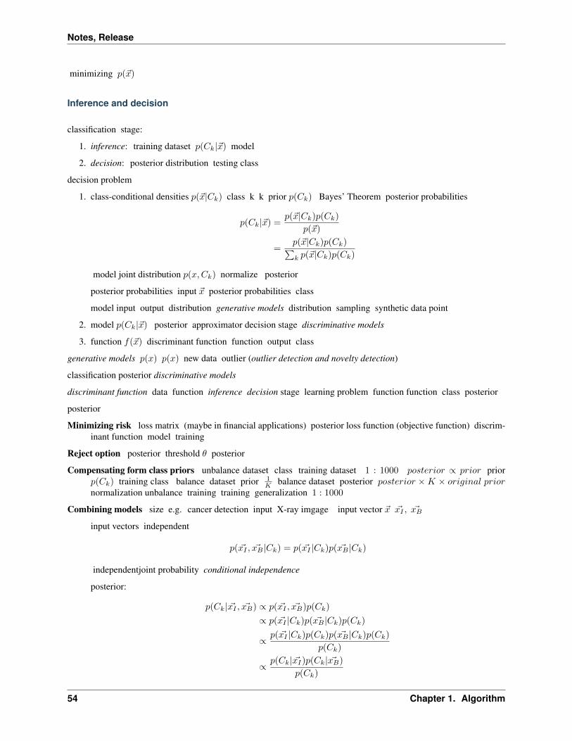
Inference and decision

classification stage:

1. inference: training dataset 𝑝(𝐶𝑘|) model

2. decision: posterior distribution testing class

decision problem

1. class-conditional densities 𝑝(|𝐶𝑘) class k k prior 𝑝(𝐶𝑘) Bayes’ Theorem posterior probabilities

𝑝(𝐶𝑘|) =𝑝(|𝐶𝑘)𝑝(𝐶𝑘)

𝑝()

=𝑝(|𝐶𝑘)𝑝(𝐶𝑘)∑𝑘 𝑝(|𝐶𝑘)𝑝(𝐶𝑘)

model joint distribution 𝑝(𝑥,𝐶𝑘) normalize posterior

posterior probabilities input posterior probabilities class

model input output distribution generative models distribution sampling synthetic data point

2. model 𝑝(𝐶𝑘|) posterior approximator decision stage discriminative models

3. function 𝑓() discriminant function function output class

generative models 𝑝(𝑥) 𝑝(𝑥) new data outlier (outlier detection and novelty detection)

classification posterior discriminative models

discriminant function data function inference decision stage learning problem function function class posterior

posterior

Minimizing risk loss matrix (maybe in financial applications) posterior loss function (objective function) discrim-inant function model training

Reject option posterior threshold 𝜃 posterior

Compensating form class priors unbalance dataset class training dataset 1 : 1000 𝑝𝑜𝑠𝑡𝑒𝑟𝑖𝑜𝑟 ∝ 𝑝𝑟𝑖𝑜𝑟 prior𝑝(𝐶𝑘) training class balance dataset prior 1

𝐾 balance dataset posterior 𝑝𝑜𝑠𝑡𝑒𝑟𝑖𝑜𝑟 ×𝐾 × 𝑜𝑟𝑖𝑔𝑖𝑛𝑎𝑙 𝑝𝑟𝑖𝑜𝑟normalization unbalance training training generalization 1 : 1000

Combining models size e.g. cancer detection input X-ray imgage input vector 𝑥𝐼 , 𝑥𝐵

input vectors independent

𝑝(𝑥𝐼 , 𝑥𝐵 |𝐶𝑘) = 𝑝(𝑥𝐼 |𝐶𝑘)𝑝(𝑥𝐵 |𝐶𝑘)

independentjoint probability conditional independence

posterior:

𝑝(𝐶𝑘|𝑥𝐼 , 𝑥𝐵) ∝ 𝑝(𝑥𝐼 , 𝑥𝐵)𝑝(𝐶𝑘)

∝ 𝑝(𝑥𝐼 |𝐶𝑘)𝑝(𝑥𝐵 |𝐶𝑘)𝑝(𝐶𝑘)

∝ 𝑝(𝑥𝐼 |𝐶𝑘)𝑝(𝐶𝑘)𝑝(𝑥𝐵 |𝐶𝑘)𝑝(𝐶𝑘)

𝑝(𝐶𝑘)

∝ 𝑝(𝐶𝑘|𝑥𝐼)𝑝(𝐶𝑘|𝑥𝐵)

𝑝(𝐶𝑘)


Notes, Release

posterior posterior training data (𝑝(𝐶𝑘)) normalization posterior

naive Bayesian model conditional independent

Loss functions for regression

𝐸(𝐿) =

∫ ∫𝐿(𝑡, 𝑦())𝑝(, 𝑡)𝑑𝑑𝑡∫ ∫

𝑓(·)𝑑𝑑𝑡 𝑑 𝑑𝑡 𝑓(·)

𝐿(𝑡, 𝑦()) = (𝑦()− 𝑡)2 square lose function

𝐸(𝐿) =

∫ ∫(𝑦()− 𝑡)2𝑝(, 𝑡)𝑑𝑑𝑡

minimizing 𝑦(𝑥) (model)

Information Theory

discrete random variable 𝑥 , .

𝑥

probability distribution 𝑝(𝑥) , Monotonic function ℎ(𝑥) x information gain suprise

𝑥, 𝑦 (independent) random variable, ℎ(𝑥, 𝑦) :

ℎ(𝑥, 𝑦) = ℎ(𝑥) + ℎ(𝑦)

:

𝑝(𝑥, 𝑦) = 𝑝(𝑥)𝑝(𝑦)

:

ℎ(𝑥) = − log2 𝑝(𝑥)

ℎ(𝑥) >= 0

𝑥 , :

𝐻(𝑥) =∑𝑥

𝑝(𝑥)ℎ(𝑥)

= −∑𝑥

𝑝(𝑥) log2 𝑝(𝑥)

𝑒𝑛𝑡𝑟𝑜𝑝𝑦

Continueous Var

𝑒𝑛𝑡𝑟𝑜𝑝𝑦 Continueous variable

𝐻() = −∫𝑝() ln 𝑝()𝑑

differential entropy

1.6. PRML 55

https://en.wikipedia.org/wiki/Monotonic_function

Notes, Release

Mutual Information

random variablesdependent

random variables share variable

𝐼(𝑋;𝑌 ) =∑𝑥∈𝑋

∑𝑦∈𝑌

𝑝(𝑥, 𝑦) log( 𝑝(𝑥, 𝑦)

𝑝(𝑥)𝑝(𝑦)

)random variable independent

log( 𝑝(𝑥, 𝑦)


)= log

(𝑝(𝑥)𝑝(𝑦)


)= log 1 = 0

1.6.2 Probability Distributions

density estimation random variable 𝑋 , random variable is a function, 𝑥1, 𝑥2, . . . , 𝑥𝑛 probability distribution 𝑝(𝑋)

Assumption data points i.i.d. (independent and identically distribution)

ill-posed problem density estimation problem ill-posed – probability distribution model selection

parametric distribution distribution data

non-parametric density estimation parametric distribution distribution data set data set

Bernoulli Distribution

state

𝑥 ∈ 0, 1

Let 𝑝(𝑥 = 1|𝜇) = 𝜇

𝑝(𝑥 = 0|𝜇) = 1− 𝜇

distribution

𝐵𝑒𝑟𝑛(𝑥|𝜇) = 𝜇𝑥(1− 𝜇)(1− 𝑥)

∴ 𝐵𝑒𝑟𝑛(𝑥 = 1|𝜇) = 𝜇1(1− 𝜇)0

= 𝜇

∴ 𝐵𝑒𝑟𝑛(𝑥 = 0|𝜇) = 𝜇0(1− 𝜇)1

= (1− 𝜇)

dataset 𝒟 = 𝑥1, . . . , 𝑥𝑛 iid Likelihood function

𝑝(𝒟|𝜇) =

𝑁∏𝑛

𝑝(𝑥𝑛|𝜇)

=

𝑁∏𝑛

𝜇𝑥𝑛(1− 𝜇)(1− 𝑥𝑛)

Then, log likelihood function

ln 𝑝(𝒟|𝜇) =

𝑁∑𝑛

ln 𝑝(𝑥𝑛|𝜇)

=

𝑁∑𝑛

ln(𝜇𝑥𝑛(1− 𝜇)(1− 𝑥𝑛)

)


Notes, Release

maximum likelihood

𝜇𝑀𝐿 =1

𝑁

𝑁∑𝑛

𝑥𝑛

1 average

1.6.3 Classification

Discriminant Function

Two Classes

𝑦(𝑥) = 𝑇𝑥+ 𝑤0

𝑤0 is bias, sometimes a negative 𝑤0 is called threshold

Multiple Classes

problem 3 one-versus-the-rest classifier hyperplane feature space decision boundary boundary 4decision region 3 testing (p183. Figure 4.2)

sol Single K-class discriminant function, K

𝑦𝑘() = 𝑤𝑘𝑇 + 𝑤𝑘0

e.g. 3 𝐶1, 𝐶2, 𝐶3 ⎧⎪⎨⎪⎩𝑦1() = 𝑤1

𝑇 + 𝑤10

𝑦2() = 𝑤2𝑇 + 𝑤20

𝑦3() = 𝑤3𝑇 + 𝑤30

Let ∈ 𝐶𝑘 if 𝑦𝑘 > 𝑦𝑗 ,∀𝑗 = 𝑘

Decision boundary 𝑦𝑘 = 𝑦𝑗 ⎧⎪⎨⎪⎩𝑦1 = 𝑦2

𝑦2 = 𝑦3

𝑦3 = 𝑦1

=⇒

⎧⎪⎨⎪⎩𝑦1 − 𝑦2 = 0

𝑦2 − 𝑦3 = 0

𝑦3 − 𝑦1 = 0

→ (𝑤𝑘 − 𝑤𝑗)𝑇 + (𝑤𝑘0 − 𝑤𝑗0) = 0

Perceptron

Perceptron criterion

1.6. PRML 57

Notes, Release

𝑤𝑇 (𝑥𝑛)𝑡𝑛 > 0

E SGD iter

converge: 𝐸(𝑤(𝑡+ 1)) < 𝐸(𝑤)

(4.57) (4.57) sigmoid function

(4.72) log

Section name

maximum likelihood

4.2.1 why gaussian?

what is share variance?

Discriminative Model

model linear maximum posterior

4.87

logistic function posterior

(4.89) likelihood 𝑦𝑛 posterior

(4.91) cross-entropy (?) entropy (4.91) AKA cross-entropy error function

sigmoid function 𝑑𝜎𝑑𝑎=𝜎(1−𝜎)

IRLS

Newton-Raphon method

( Gradient Descent )

Generative Model and Discriminative Model

• 𝐶𝑘, 𝑘 ∈ 1, 2 output

• 𝑋 ∈ 𝑥1, . . . , 𝑥𝑛 data, input

Naive Bayes classifier Logistic Regression

• Naive Bayes Generative Model

• Logistic Regression Discriminative Model

Naive Bayes classifier

posterior data class 𝑝(𝐶𝑘|𝑋 = 𝑥𝑛+1) posterior


https://en.wikipedia.org/wiki/Naive_Bayes_classifier

Notes, Release

Build model :

𝑝(𝐶𝑘 = 1|𝑋) =𝑝(𝐶𝑘 = 1, 𝑋)

𝑝(𝑋)

𝑝(𝐶𝑘 = 2|𝑋) =𝑃 (𝐶𝑘 = 2, 𝑋)

𝑝(𝑋)

𝑝(𝑋) model joint probability

𝑝(𝐶𝑘 = 1, 𝑋) = 𝑝(𝑋|𝐶𝑘 = 1)𝑝(𝐶𝑘 = 1)

𝑝(𝐶𝑘 = 2, 𝑋) = 𝑝(𝑋|𝐶𝑘 = 2)𝑝(𝐶𝑘 = 2)

𝑝(𝑋|𝐶𝑘)

𝑝(𝑋|𝐶𝑘 = 1) =

⎧⎪⎨⎪⎩𝑝(𝑋 = 𝑥1|𝐶𝑘 = 1)

. . .

𝑝(𝑋 = 𝑥𝑛|𝐶𝑘 = 1)

𝑝(𝑋|𝐶𝑘 = 2) =

⎧⎪⎨⎪⎩𝑝(𝑋 = 𝑥1|𝐶𝑘 = 2)

. . .

𝑝(𝑋 = 𝑥𝑛|𝐶𝑘 = 2)

Naive Bayes 𝑝(𝑋|𝐶𝑘)

Logistic Regression

model linear model

posterior formula

𝑝(𝐶𝑘 = 1|𝑋) = . . .

𝑝(𝐶𝑘 = 2|𝑋) = . . .

1.6.4 Neural Networks

Raidial Based Function Networks

Gaussian Function

gaussian function 𝛼 = 1

𝛽, 𝛾 𝜇, 𝜎 e.g. k-means 𝜇, 𝜎

𝑘 = 10 RBF neuron vector 𝑘

RBF neuron gaussian function

• input vector 2e.g. (𝑥1, 𝑥2)

• RBF neuron vector 10

• input RBF neuron 10 coding

• RBF output full connected NN

1.6. PRML 59

Notes, Release

1.6.5 Kernel Method

kernel function simularity or covariance(inner product) ... etc.

memory-based method

kernel

homogeneous kernel AKA. radial-basis function

𝑘(‖𝑣𝑒𝑐𝑥− 𝑣𝑒𝑐𝑥′‖)

Dual Representation

Constructing Kernel

model selection

Guassian Kernel (6.23) homogeneous kernel,

Probabilistic generative kernel

𝑘(𝑥, 𝑥′) = 𝑝(𝑥)𝑝(𝑥′)

i

𝑘(𝑥, 𝑥′) =∑𝑥

𝑝(𝑥|𝑖)𝑝(𝑥′|𝑖)𝑝(𝑖)

Fisher Kernel

(6.33)

Radial Basis Fcuntion Network

Guassian Process

Process drichlet process

Regerssion

𝑡𝑛 = 𝑦𝑛 + 𝑒𝑟𝑟𝑜𝑟𝑛

error random variable 𝜇 = 0 Guassian

𝑝(𝑡𝑛|𝑦𝑛) = 𝑁(𝑥𝑛|𝑦𝑛, 𝛽−1)

𝑝(𝑡𝑛+1|𝑡𝑁 )


Notes, Release

1.6.6 Graphical Models

• probabilistic graphical models

probabilistic graphical models node ( vertex ) random variable(s) link ( edage ) graph node joint probability

Quote:

For the purposes of solving inference problems, it is often convenient to convert both directed and undi-rected graphs into a different representation called a factor graph.

Bayesian Network

Aka. Belief Network

Family Directed Graphical Models:

Markov Random Fields

Family Undirected Graphical Models

1.6.7 Misc

1.7 Reinforcement Learning

1.7.1 Overview

agent OR LR approximate dynamic programming ML LR economic (bounded rationality)

ML Markov decision process (MDP), dynamic programming

Reinforcement Learning and Markov Decision Processes

1. supervised learning unsupervised learning

2. sequential decision making problem

3. environment system state actions + states

4. “sequential decision making can be viewed as instances of MDPs.”

5. policy a function maps state into actions.

6. decision making problem * rule base – programming

• search and planning

• probabilistic planning algorithms

• learning

7. Online –

8. Offline – simulator

1.7. Reinforcement Learning 61

Notes, Release

Credit Assignment

training credit contribute credit ?

temporal credit assignment problem

structural credit assignment problem (?) agent policy function e.g. NN params update NN structural creditassignment problem

Exploration-Exploitation Trade-off

Exploration

Exploitation

Performance

• RL performance measurement stochastic, policy update

concept drift

• supervised/unsupervised learning data prior distribution

• subgoals

Markov Decision Process

• stochastic extension of finite automata

• MDP infinite

• key componement

– states

– actions

– transitions

– reward function

States

A finite set 𝑆 = 𝑠1, . . . , 𝑠𝑁

The size of set space is 𝑁 . ‖𝑆‖ = 𝑁

use features to describe a state

Actions

A finite set 𝐴 = 𝑎1, . . . , 𝑎𝐾

‖𝐴‖ = 𝐾

Actions can control the system states.

action state : 𝐴(𝑠)


Notes, Release

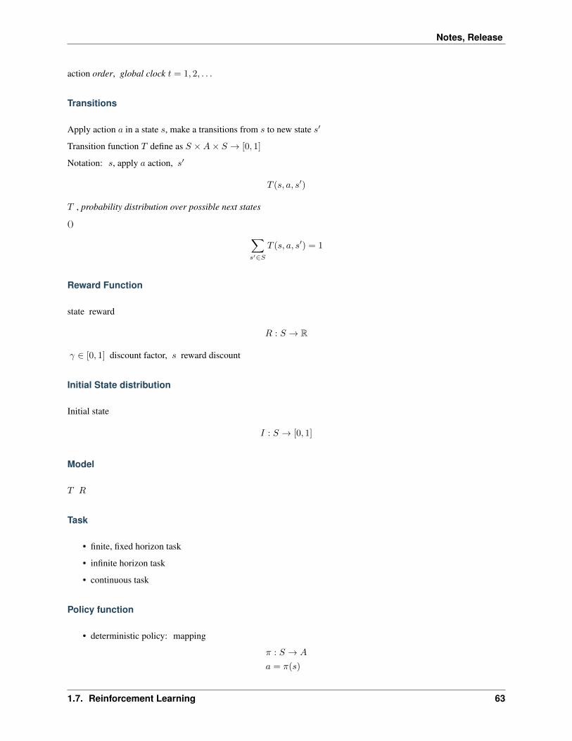
action order, global clock 𝑡 = 1, 2, . . .

Transitions

Apply action 𝑎 in a state 𝑠, make a transitions from 𝑠 to new state 𝑠′

Transition function 𝑇 define as 𝑆 ×𝐴× 𝑆 → [0, 1]

Notation: 𝑠, apply 𝑎 action, 𝑠′

𝑇 (𝑠, 𝑎, 𝑠′)

𝑇 , probability distribution over possible next states

() ∑𝑠′∈𝑆

𝑇 (𝑠, 𝑎, 𝑠′) = 1

Reward Function

state reward

𝑅 : 𝑆 → R

𝛾 ∈ [0, 1] discount factor, 𝑠 reward discount

Initial State distribution

Initial state

𝐼 : 𝑆 → [0, 1]

Model

𝑇 𝑅

Task

• finite, fixed horizon task

• infinite horizon task

• continuous task

Policy function

• deterministic policy: mapping

𝜋 : 𝑆 → 𝐴

𝑎 = 𝜋(𝑠)


Notes, Release

• stochastic policy: 𝑠, 𝑎 output output 𝑎

𝜋 : 𝑆 ×𝐴→ [0, 1]

𝑎 ∼ 𝜋(𝑎|𝑠)

• parameterized policies 𝜋𝜃 𝜋 e.g. NN function approximator output

– deterministic: 𝑎 = 𝜋(𝑠, 𝜃)

– stochastic: 𝑎 ∼ 𝜋(𝑎|𝑠, 𝜃)

process policy function stationary

Optimality

agent rewardaverage or rewards,

optimality process reward , reward sum, discount, process average rewards.

Finite horizon: h ( finite horizon) rewards. h-step optimal action

𝐸[

ℎ∑𝑡=0

𝑟𝑡]

discount finite horizon discount reward:

𝐸[

ℎ∑𝑡=0

𝛾𝑡𝑟𝑡]

Sepcial case of discount finite horizon model: Immediate reward

Let 𝛾 = 0

𝐸[𝑟𝑡]

discount infinite horizon:

𝐸[

∞∑𝑡=0

𝛾𝑡𝑟𝑡]

Value Function

link optimality and policy.

algo learning target:

• value function, aka critic-based algorithms

– Q-Learning

– TD-Learning

• actor-based algorithms

agent state (how good in certain state)

optimality criterion e.g. average rewords “The notion of how good is expressed in terms of an optimality crite-rion, i.e. in terms of the expected return.”

𝜋 hyper parameter? “Value functions are defined for particular policies.”


Notes, Release

input 𝑠 𝜋 “value of a state 𝑠 under policy 𝜋“

𝑉 𝜋(𝑠)

e.g. optimality finite-horizon, discounted model, given policy 𝜋, state 𝑠

𝑉 𝜋(𝑠) = 𝐸𝜋[

ℎ∑𝑘=0

𝛾𝑘𝑟𝑡+𝑘|𝑠𝑡 = 𝑠]

𝑟𝑡+𝑘 𝑡 𝑘

state-action value function 𝑄 : 𝑆 ×𝐴→ R

state 𝑠, 𝜋 𝑎

𝑄𝜋(𝑠, 𝑎) = 𝐸𝜋[

ℎ∑𝑘=0

𝛾𝑘𝑟𝑡+𝑘|𝑠𝑡 = 𝑠, 𝑎𝑡 = 𝑎]

Bellman Equation

Aka. Dynamic Programming Equation

discrete-time

e.g. (𝑣.1) sum Bellman Equation

𝑉 𝜋(𝑠) = 𝐸𝜋[𝑟𝑡 + 𝛾𝑟𝑡+1 + 𝛾2𝑟𝑡+2 + . . . |𝑠𝑡 = 𝑡] (1.19)= 𝐸𝜋[𝑟𝑡 + 𝛾𝑉 𝜋(𝑠𝑡+1)|𝑠𝑡 = 𝑠](1.20)

=∑𝑠′

𝑇 (𝑠, 𝜋(𝑠), 𝑠′)

(𝑅(𝑠, 𝑎, 𝑠′) + 𝛾𝑉 𝜋(𝑠′)

)(1.21)

Expectation transition probabilistic sum Expectation Immediate reward + value of next step

:optimal 𝜋: 𝜋*

:optimal 𝑉 : 𝑉 𝜋*

= 𝑉 *

Bellman optimality equation

𝑉 *(𝑥) = max𝑎∈𝐴

∑𝑠′∈𝑆

𝑇 (𝑠, 𝜋(𝑠), 𝑠′)

(𝑅(𝑠, 𝑎, 𝑠′) + 𝛾𝑉 𝜋(𝑠′)

)

𝜋*(𝑠) = arg max𝑎

∑𝑠′∈𝑆

𝑇 (𝑠, 𝜋(𝑠), 𝑠′)

(𝑅(𝑠, 𝑎, 𝑠′) + 𝛾𝑉 𝜋(𝑠′)

)policy greedy policy deterministic value function best action

optimal state-action value function:

𝑄*(𝑠, 𝑎) =∑𝑠′

𝑇 (𝑠, 𝑎, 𝑠′)

(𝑅(𝑠, 𝑎, 𝑠′) + 𝛾max

𝑎′𝑄*(𝑠′, 𝑎′)

)state-action policy stochastic policy max𝑎′ 𝑄

* 𝑄 next action

∵∑𝑎′∈𝐴

𝜋(𝑠′, 𝑎′) = 1

stochastic


Notes, Release

Model-based and Model-free

Model model of MDP MDP (𝑆,𝐴, 𝑇,𝑅) 𝑇 𝑅 environment

Model-based algorithms “Model-based algorithms exist under the general name of DP.” DP prioragent env data model model DP Bellman Equation optimal policy

Model-free algorithms “Model-free algorithms, under the general name of RL” model 𝑇, 𝑅 agentpolicy 𝑇, 𝑅

“a simulation of the policy thereby generating samples of state transitions and rewards.”

state-action function (e.g. Q-function)

Q function model-free approach T R model T R method model-free algorithms

“Q-functions are useful because they make the weighted summation over different alternatives (such as inEquation v.1) using the transition function unnecessary. This is the reason that in model-free approaches,i.e. in case T and R are unknown, Q-functions are learned instead of V-functions.”

T R MDP framework policy agent

Relation between 𝑄* and 𝑉 *

𝑉 *(𝑠) = max𝑎

𝑄*(𝑠, 𝑎)

𝑄*(𝑠, 𝑎) =∑𝑠′

𝑇 (𝑠, 𝑎, 𝑠′)

(𝑅(𝑠, 𝑎, 𝑠′) + 𝛾𝑉 *(𝑠′)

)𝜋*(𝑠) = arg max

𝑎𝑄*(𝑠, 𝑎)

Generalized Policy Iteration (GPI)

Two steps:

• policy evaluation: 𝜋 𝑉 𝜋

• policy improvement: state action 𝜋 states action state 𝜋 action

𝑉 𝜋 improve 𝜋 𝜋′

value function policy state case model-free (?)

“Note that it is also possible to have an implicit representation of the policy, which means that only thevalue function is stored, and a policy is computed on-the-fly for each state based on the value functionwhen needed.”

value function

Dynamic Programming

DP model optimal policies “The term DP refers to a class of algorithms that is able to compute optimal policies inthe presence of a perfect model of the environment.”


Notes, Release

Fundamental DP Algorithms

Two core method:

• policy iteration

• value iteration

Policy Iteration

Policy Evaluation stage

decision theorem inference stage stage policy 𝜋

value function 𝑉 𝜋 (given a fixed policy 𝜋).

MDP model 𝑉 𝜋 𝑆. linear programming

iterative Bellman Equation update rule: state 𝑠′ horizon 𝑉 𝜋𝑘 𝑉 𝜋𝑘+1 ← 𝐹 [𝑉𝑘(𝑠′)]

𝑉 𝜋𝑘+1 horizon 𝑘 + 1, 𝑉 𝜋𝑘 𝑘 𝑉 𝜋 infinite-horizon

𝑉 𝜋𝑘+1(𝑠) = 𝐸𝜋[𝑟𝑡 + 𝛾𝑟𝑡+1 + · · ·+ 𝛾𝑘+1𝑟𝑡+𝑘+1]

= 𝐸𝜋[𝑟𝑡 + 𝛾(𝑟𝑡+1 + · · ·+ 𝛾𝑘𝑟𝑡+𝑘+1

)]

= 𝐸𝜋[𝑟𝑡 + 𝛾𝑉 𝜋𝑘 (𝑠′)]

=∑𝑠′

𝑇 (𝑠, 𝜋(𝑠), 𝑠′)(𝑅(𝑠, 𝜋(𝑠), 𝑠′) + 𝛾𝑉 𝜋𝑘 (𝑠′)

)iteration 𝑘, 𝑘 = 1 : inf 𝑘 DP

iteration 𝑘 iter 𝑠 𝑠 full backup transition probabilities

general formulation backup operator 𝐵𝜋 over 𝜑 𝜑 map state space e.g. 𝜑 value function

(𝐵𝜋𝜑)(𝑠) =∑𝑠′∈𝑆

𝑇 (𝑠, 𝜋(𝑠), 𝑠′)(𝑅(𝑠, 𝜋(𝑠), 𝑠′) + 𝛾𝜑(𝑠′)

)optimal value function 𝑉 *objective function

𝑉 * = arg max𝑉

∑𝑠∈𝑆′

𝑉 (𝑠)

s.t.∀𝑎,∀𝑠, 𝑉 (𝑠) ≥ (𝐵𝑎𝑉 )(𝑠)

𝐵𝑎𝑉 action

Policy Improvement stage

policy, s.t. 𝑉 𝜋1(𝑠) ≥ 𝑉 𝜋0(𝑠),∀𝑠 ∈ 𝑆

𝜋0 policy e.g ...etc

Pseudo code:

k = 1 # horizonpi[1] = ... # baseline policy

while not converge


Notes, Release

# policy evaluationfor s in S

pi[k, ...] = ...end

# policy improvementfor s in S

pi[k+1, ...] = indmax(...)end

k += 1end

Updating style

Sync A.k.a Jacobi-style table

In-place

Async extend of in-place, but in any order.

Modified policy iteration (MPI)

Two steps:

• policy evaluation

• policy improvement

It’s general method of async update

Heuristics and Search

Heuristics general async DP

Goal-based reward function goal state positive reward

RL

Model-free MDP with approximation and incomplete information sampling exploration

transition model prior reword function prior

model-free

• transition and reward models model DP indircet RL or model-based RL

• direct RL action value model

• “For example, one can still do model-free estimation of action values, but use an approximated model tospeed up value learning by using this model to perform more, and in addition, full backups of values(see Section 1.7.3).”“


Notes, Release

Temporal Difference Learning

TD learning episode update value 30 update

TD algo bootstrapping

TD(0)

policy function 𝜋 𝑉 𝜋 online RL

𝑉𝑘+1(𝑠)← 𝑉𝑘(𝑠) + 𝛼(𝑟 + 𝛾𝑉𝑘(𝑠′)− 𝑉𝑘(𝑠))

𝛼 learning rate

Note: learning rate 𝛼 fixed s’ s’ learning rate 𝛼(𝑠)

update rule transition update DP full backup experience simple backup

𝑉𝑘+1 𝑠′ iter state space

testing phase value function 𝑉 𝜋 action selection

𝜋(𝑠) = arg max𝑎

∑𝑠

𝑅(𝑠, 𝑎) + 𝑉 (𝑠)

𝑠′ experience DP expectation over transition distribution

Q-Learning

Model-free

Q function state-action value function

𝑄 : (𝑠, )→ R

infinite horizon Q function

TD(0) Q function sampling action selection transition model

Hyper Parameters

• 𝛾 discount factor

• 𝛼 learning rate

Initialization

• baseline (arbitrarily or trivial) 𝑄

• e.g. 𝑄(𝑠, 𝑎) = 0,∀𝑠 ∈ 𝑆, ∀𝑎 ∈ 𝐴

function choose_action()if exploration

random actionelse

base on current Qend

end


Notes, Release

for each episodes <- starting state

while (s' != goal state)a <- choose_action()perform action a

Q(s, a) <- Q(s, a) + 𝛼(r + 𝛾 max Q(s', a') - Q(s, a))s <- s'

endend

Off-policy Q max operator episode

“while following some exploration policy 𝜋, it aims at estimating the optimal policy 𝜋*“

SARSA

State-Action-Reward-State-Action

Update rule:

𝑄𝑡+1(𝑠𝑡, 𝑎𝑡) = 𝑄𝑡(𝑠𝑡, 𝑎𝑡) + 𝛼(𝑟𝑡 + 𝛾𝑄𝑡(𝑠𝑡+1, 𝑎𝑡+1)−𝑄𝑡(𝑠𝑡, 𝑎𝑡))

On-policy action 𝑎𝑡+1 𝜋(𝑠𝑡+1) Q-learning max operator max operator action Q value

Q SARSA

SARSA non-stationary

Actor-Critic Learning

On-policy policy value function

Actor Policy function

Critic Value function state-value function 𝑉

action selection critic TD-error action

𝛿𝑡 = 𝑟𝑡 + 𝛾𝑉 (𝑠𝑡 + 1)− 𝑉 (𝑠𝑡)

preference of an action 𝑎 in state 𝑠 defined as 𝑝(𝑠, 𝑎), update rule:

𝑝(𝑠𝑡, 𝑎𝑡) < −𝑝(𝑠𝑡, 𝑎𝑡) + 𝛽𝛿𝑡

TD-error / action preference preference update rule actor-critic method policy prior

Monte Carlo Method

unbiased estimate

𝑇𝐷(𝜆) where 𝜆 = 1 Monte Carlo


Notes, Release

Reference

• https://en.wikipedia.org/wiki/Reinforcement_learning

• https://www.quora.com/What-is-the-difference-between-model-based-and-model-free-reinforcement-learning

• https://ocw.mit.edu/courses/aeronautics-and-astronautics/16-410-principles-of-autonomy-and-decision-making-fall-2010/lecture-notes/MIT16_410F10_lec23.pdf

1.7.2 Batch Reinforce Learning

Pure Batch RL

Three phase

1. experience

• purely random action

• agent

• experience set ℱ = (𝑠, 𝑎, 𝑟′, 𝑠′) . . . experience

2. Learning stage

• experience set prior

• experience set optimal policy

3. Application

purely random (uniformed policy) state goal state states

Growing Batch RL

Modern batch RL pure batch pure online

Foundations of Batch RL Algorithms

Q-Learning Q learning system Q Q table discrete state space state space

• exploration overhead

• stochastic approximation

• function approximation

Experience Replay

pure online Q-Learning current optimal action exploration -greedy state Q table greedy greedy policy transitiontuple (𝑠, 𝑎, 𝑟, 𝑠′) update 𝑄′(𝑠, 𝑎) table “local” update

experience replay exploration overhead.

experience replay growing batch problem

experience n experience apply update rule n iter experience back-propagate


https://en.wikipedia.org/wiki/Reinforcement_learning

https://www.quora.com/What-is-the-difference-between-model-based-and-model-free-reinforcement-learning

https://ocw.mit.edu/courses/aeronautics-and-astronautics/16-410-principles-of-autonomy-and-decision-making-fall-2010/lecture-notes/MIT16_410F10_lec23.pdf

https://ocw.mit.edu/courses/aeronautics-and-astronautics/16-410-principles-of-autonomy-and-decision-making-fall-2010/lecture-notes/MIT16_410F10_lec23.pdf

Notes, Release

Stability Issues

Idea of Fitting

Online RL asynchronous updates state state

Q table discrete case update state-action pair

Idea of Fitting function approximation

𝑓 ′(𝑠, 𝑎) = 𝑓(𝑠, 𝑎) + 𝛼(𝑟 + max𝑎′∈𝐴

𝑓(𝑎′, 𝑠′)− 𝑓(𝑠, 𝑎))

= 𝑓(𝑠, 𝑎) + 𝛼(𝑞𝑠,𝑎 − 𝑓(𝑠, 𝑎))

update structuree.g reward ...etc

Fitting update rule

Stable Function Approximation in Dynamic Programming

function approximator TD methods K-nearest-nieghbor, linear interpolation(?), local weight averaging approxima-tion

Algo:

1. a set of 𝑠 ∈ 𝑆 (state space) set 𝐴. 𝑠 distribution sampling state space sampling supports.

2. Initial guess value function 𝑉0

3. 𝑀𝐴 learning algorithm training set 𝐴 𝑓(𝐴) training set labels

𝑀𝐴(𝑓(𝐴), 𝐴)→ 𝑓

𝑀𝐴 label training data function approximator (e.g. a neural nets) 𝑓

4. iteration

𝑉 0

𝑉 1 ←𝑀𝐴(𝑉 0, 𝐴0)

𝐴1 ← 𝑇𝐴(𝑉 1)

(sampling)

𝑉 2 ←𝑀𝐴(𝑉 1, 𝐴1)

. . .

Replace Inefficient Stochastic Approximation

fitting model-free-sample-based

Ormoneit (2002) random sampling supports 𝑓 sampled transition + kernel-based approximator 𝑓

transition samples (a set of state-action pair) (given current state) transition value e.g. transition value averaging (orkernel-based averaging)

Ormoneit averaging transition model this implies from random sampling to the true distribution.


Notes, Release

Batch RL Algorithms

Ormoneit kernel-based framework

kernel-based approximate dynamic programming (KADP)

• experience replay

• fitting

• kernel-based self-approximation (sample-based)

Kernel-Based Approximate Dynamic Programming

Bellman equation function

𝑉 = 𝐻𝑉

𝑉 = 𝑉

𝐻 DP-operator

Iteration process, where 𝑉 0 is the initial guess:

𝑉 𝑖+1 = 𝑉 𝑖

where = 𝐻𝑚𝑎𝑥𝑎𝑑𝑝

∴ 𝑉 𝑖+1 = 𝐻𝑚𝑎𝑥𝑎𝑑𝑝𝑉

𝑖

with a given exp set

𝐹 = (𝑠𝑡, 𝑎𝑡, 𝑟𝑡+1, 𝑠𝑡+1)|𝑡 = 1 . . . 𝑝

𝑎𝑑𝑝𝑉

𝑖

𝑎𝑑𝑝𝑉

𝑖 =∑

(𝑠,𝑎,𝑟,𝑠′)∈𝐹𝑎

𝑘(𝑠, 𝜎)(𝑟 + 𝛾𝑉 𝑖(𝑠′)

)=⇒ 𝑖+1

𝑎 (𝜎) =∑

(𝑠,𝑎,𝑟,𝑠′)∈𝐹𝑎

𝑘(𝑠, 𝜎)(𝑟 + 𝛾max

𝑎′∈𝐴𝑖(𝑠′, 𝑎′)

)𝐹𝑎 given 𝑎 set 𝑖+1

𝑎 given 𝑎

Bellman equation max operator

𝑉 𝑖+1(𝑠) = 𝐻𝑚𝑎𝑥𝑖+1𝑎 (𝑠)

= max𝑎∈𝐴

𝑖+1𝑎 (𝑠)

policy argmax

𝜋(𝑠) = arg max𝑎∈𝐴

𝑉 𝑖+1(𝑠)

policy update rule

𝜋𝑖+1(𝜎) = arg max𝑎∈𝐴

𝑉 𝑖+1(𝜎)

= arg max𝑎∈𝐴

∑(𝑠,𝑎,𝑟,𝑠′)∈𝐹𝑎

𝑘(𝑠, 𝜎)(𝑟 + 𝛾max

𝑎′∈𝐴𝑖(𝑠′, 𝑎′)

)Constrain from kernel: ∑

𝐹𝑎

𝑘(𝑠, 𝜎) = 1, ∀𝜎 ∈ 𝑆


Notes, Release

Kernel-Based Reinforcement Learning

• Ormoneit (2002)

continuous state-space TD parametric function approximator (e.g neural nets, linear regression) Bellman equationinitialization value bias reinforcement learning algorithm e.g bias regression problem

Bias-variance tradeoff

• bias: underfitting

• variance: overfitting

• discounted-cost problem

• average-cost problemOrmoneit & Glynn (2002)

Kernel-based averaging (inspired by idea of local averaging).

MDP setting

• discrete time steps 𝑡 = 1, 2, . . . 𝑇


CHAPTER 2

Database

2.1 Cloudant

CouchDB is the database for hackers. The philosophy of design is totally different from Mongo.

CouchDB let application built/stored inside database (via design document). And hackers can make a customizedquery server to create magical data service!

2.1.1 REST API

The REST api is stateless. Thus, there is no cursor.

/_all_docs

sorted key list

GET

params:

• startkey

• endkey

• include_doc=(true|false) false

• descending=(true|false) false

• limit=N

• skip=N

75

Notes, Release

2.1.2 Replication

CouchDB developes a well-defined replication protocol.

• Only sync on differ, including change history, deleted docs.

• compression through transfer

Master To Master

CouchDB can just setup replicator on both end to achieve this.

Single Replication

For the snapshot of database

_local doc

The doc recorded in _local won’t be sent through replication.

API

METHOD /database/_local/id

Alternative

If we want to use including method, we can use docs_id in replication doc:

doc_ids (optional) Array of document IDs to be synchronized

Replicator Database

The field _replication_state always is triggered, if this replication is set to continue.

Idea

We can build a application understanding this protocol to

1. make a backup service

2.1.3 Revision

limits

CouchDB can track document’s revsion up to 1000 (default limit, configurable)

$ curl "http://server/db/_revs_limit"1000

76 Chapter 2. Database

Notes, Release

Get revisions list

$ curl "http://server/db/doc?revs=true"

$ curl "http://server/db/doc?revs_info=true"

2.1.4 Secondary index

MapReduce

• Unable to join between documents

Map Function

map() -> (key, val)

• build-in MapReduce fnuctions was written in Erlang -> faster

reduce function can be group by key

• pi?group=true

• api?group_level=N

multiple emit

function(doc)

emit(doc.id, 1);emit(doc.other, 2);

GET

reduce true|false

group true|false

stale ok -> optional skip index building

group_level key in [k1, k2, k3]

group_level=1 -> group by [k1]

group_level=2 -> group by [k1, k2]

Reduce Function

if rereduce is False:

reduce([

[key1, id1],[key2, id2],[key3, id3]

],[ value1, value2, value3 ],

2.1. Cloudant 77

Notes, Release

false,)

e.g:

reduce([

[[

id,val,

],id1],

[[

id,val,

], id2],

[[

id,val,

], id3]

],[ value1, value2, value3 ],false,

)

View Group

One design doc can contain multiple view. Thus, there is a view group.

Each view group consume one Query Server(one process),

Chainable MapReduce

Add dbcopy field in design document

• cloudant only feature

TOOD ref

2.1.5 CouchApp

This is the killer feature of CouchDB.

Application can live in CouchDB.

The function defined in design documents will be run with Query Server. CouchDB self-shipped a js engine, Spider-Monkey, as default Query Server. We can customized our Query Server, also.

• It contains server-side js engine, earlier than nodejs.

• Couch Desktop


http://examples.cloudant.com/sales/_design/sales/index.html

http://www.freedesktop.org/wiki/Specifications/desktopcouch/

Notes, Release

• CouchApp can be distributed via Replication .

Query Server

Protocol

CouchDB communicate with it via stdio.

Time out

config

# to show$ curl -X GET deb/_config/couchdb

"uuid": "47a043497fb27ffd481a25671220b2c5","max_document_size": "67108864","database_dir": "/srv/cloudant/db","file_compression": "snappy","geo_index_dir": "/srv/cloudant/geo_index","attachment_stream_buffer_size": "4096","max_dbs_open": "500","delayed_commits": "false","view_index_dir": "/srv/cloudant/view_index","os_process_timeout": "5000"

# change config$ curl -X PUT deb/_config/couchdb/os_process_timeout -d '10000'

Show Function

List Function

Update Function

updatefuc(doc, req)

2.1.6 Cloudant Search

• build on Apache Lucene

• text searching

• text analyzer

• ad-hoc query

– primary index

– secondary index

• can create index on inside text

2.1. Cloudant 79

Notes, Release

Query Syntax

Lucene query syntax ref

Index Function

index('field', doc.field, options: val)

2.1.7 Cloudant Query

• JSON query syntax

• store in design doc

– primary index (out-of-box)

– type json: store json index in view.map

– search index -> type text

– lang (query server) query

2.1.8 Security

Auth

local.ini

Assume we have the following admin section with unencrypted password.

[admin]

admin = passwordfoo = bar...

And restart the cloudant/couchdb, it will auto generate encrypted password for you.

Couchdb:

$ sudo service couchdb restart

Cloudant on debian:

$ sudo sv restart /etc/service/cloudant

2.1.9 Comparison

The following table compare some method in design document.


https://lucene.apache.org/core/5_2_0/queryparser/org/apache/lucene/queryparser/classic/package-summary.html#package_description

Notes, Release

item Secondary Index Cloudant Search Cloudant QueryRequire to build index V V XSenario

• Map– doc filter-

ing– doc

reshaping– multipleemit()

• Reduce– sum– stat– count– grouping– complex

key– for

reporting• Query Server

– embededAP

– specialprotocol

– highlycus-tomized

• Search engine– keyword

search–

tokenlizer– fuzzy

search– regex– numeric value

*rangebase

• Ad-hoc query• module mango

– providemongo-likequerysyntax

• SQL-like– need to

defineschemafirst

2.1.10 Attachment

All data (whatever readable or unreadable) store in the database B-tree.

An attachment should be store under a document.

API

e.g.: We have a doc user

$ curl -X GET http://server/db/user

"id": "user",..."_attachments":

"filename": "content_type": "...",... // meta datas

2.1. Cloudant 81

Notes, Release

Create

Via PUT to

http://server/db/user/filename

2.1.11 Cluster

API

GET /_up

GET /_haproxy

GET /_haproxy_health_check

2.1.12 Idea

Create ecosystem

1. CouchApp + http://codepen.io clone app from codepen!

2. CouchApp + deck.js

Visual tool for schema discover

2.1.13 Survey

Mongo cluster

2.2 MongoDB

2.2.1 Overview

MongoDB require driver to communicate with server and transfer bson.

BSON document

Additional type info

Database

Same as database in RDBMS

Collection

It’s analogous to table. All the docs in a collection should share similar schema.


Notes, Release

2.2.2 CRUD

Query

MongoDB is quite suitable for making ad-hoc/dynamic query.

We provide large amount of (SQL-like) selectors.

Syntax

• Collection

• Query Criteria

• Modifier, e.g.: sort, limit

• Projection: The fields will be returned

e.g.:

db.users.find( // criteria'age':

'$gt': 18,

, // projection'name': true,'age': true,

)

"_id" : ObjectId("55addab1166d94c5f8952452"), "name" : "foo", "age" : 18 "_id" : ObjectId("55addade166d94c5f8952453"), "name" : "bar", "age" : 20

Selector

• Comparison: $eq, $gt, ... etc.

• Logical: $or, $and, ... etc.

• Element: $exists, $type

• Evaluation: $regex, $text, $where, ... etc.

• Geospatial: $near, ... etc.

• Array: $all, $size, ... etc.

• Comment: $comment.

• Projection: $, $slice.

Projection

• Inclusion Model:


'$gt': 18,

2.2. MongoDB 83

http://docs.mongodb.org/manual/reference/sql-comparison/

Notes, Release

, // include projection'name': true,'age': true,

)

"_id" : ObjectId("55addab1166d94c5f8952452"), "name" : "foo", "age" : 18 "_id" : ObjectId("55addade166d94c5f8952453"), "name" : "bar", "age" : 20

• Exclusion Model:


'$gt': 18,

, // exclude projection'age': false,

)

"_id" : ObjectId("55addab1166d94c5f8952452"), "name" : "foo", "status" : "A" "_id" : ObjectId("55addade166d94c5f8952453"), "name" : "bar", "status" : "B"

Modifier

• limits

• skips

• sort, this require all doc loaded in mem

Text Search

Currently supported langs

Behavior

• Each query run in single collection

• Without sort, the order returned is undefined

Cursor

The find() will return a cursor.

Iteration

1. Using cursor.next()

2. cursor.toArray()

3. cursor.forEach(callback_function)

Isolation problem Same document maybe return more than on time. We using snapshot mode to handle it.


http://docs.mongodb.org/manual/reference/text-search-languages/#text-search-languages

Notes, Release

Max Doc Size

16 MB

16+ MB -> GridFS, required driver

Update

• MongoDB natively support in-place update. Change the fields we want.

•

2.2. MongoDB 85

Notes, Release


CHAPTER 3

FreeBSD

3.1 bsd-cloudinit

3.1.1 Auto Build

Working Flow

Create a raw image file

• 1.1GB is the min requirement

$ truncate -s 1124M bsdcloudinit.raw

Link it with mdconfig(8)

$ sudo mdconfig -a -f bsdcloudinit.rawmd0

Install OS via bsdinstall

bsdinstall provide scripting to automate the whole procedure.

1. Prepare environment variables

(a) We only want kernel and base:

$ export DISTRIBUTIONS='kernel.txz base.txz'

(b) Where bsdinstall can fetch distribution files:

87

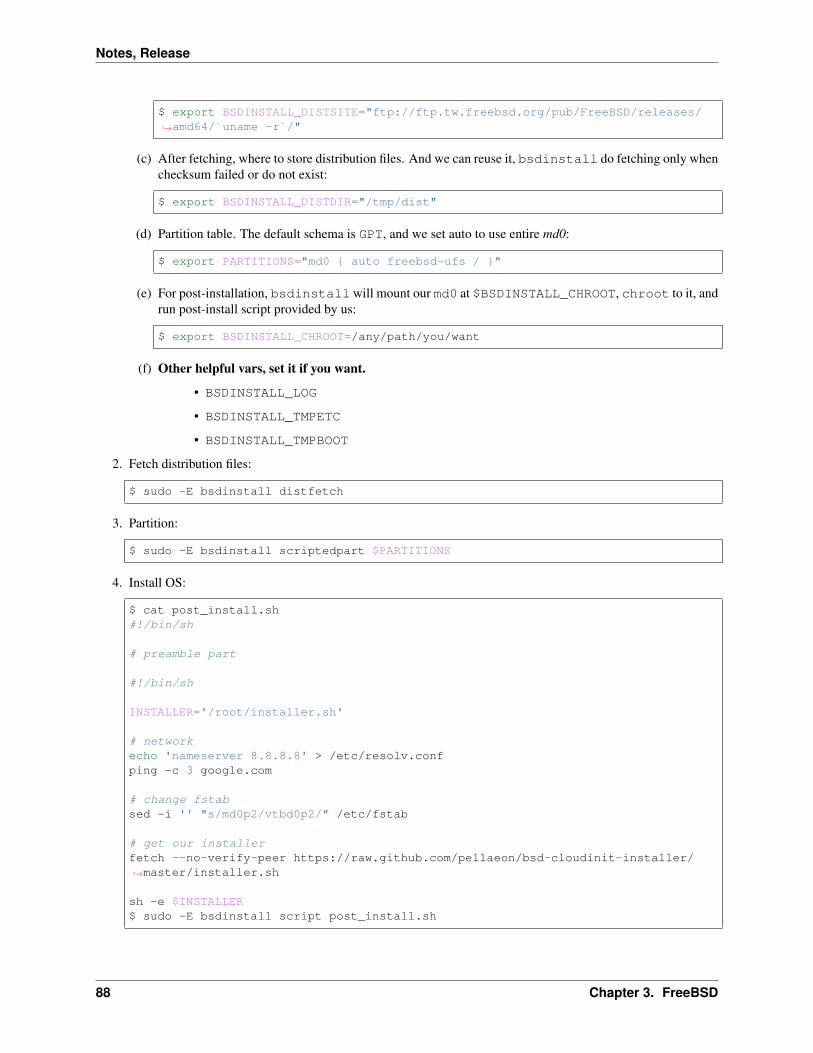
Notes, Release

$ export BSDINSTALL_DISTSITE="ftp://ftp.tw.freebsd.org/pub/FreeBSD/releases/→˓amd64/`uname -r`/"

(c) After fetching, where to store distribution files. And we can reuse it, bsdinstall do fetching only whenchecksum failed or do not exist:

$ export BSDINSTALL_DISTDIR="/tmp/dist"

(d) Partition table. The default schema is GPT, and we set auto to use entire md0:

$ export PARTITIONS="md0 auto freebsd-ufs / "

(e) For post-installation, bsdinstallwill mount our md0 at $BSDINSTALL_CHROOT, chroot to it, andrun post-install script provided by us:

$ export BSDINSTALL_CHROOT=/any/path/you/want

(f) Other helpful vars, set it if you want.

• BSDINSTALL_LOG

• BSDINSTALL_TMPETC

• BSDINSTALL_TMPBOOT

2. Fetch distribution files:

$ sudo -E bsdinstall distfetch

3. Partition:

$ sudo -E bsdinstall scriptedpart $PARTITIONS

4. Install OS:

$ cat post_install.sh#!/bin/sh

# preamble part

#!/bin/sh

INSTALLER='/root/installer.sh'

# networkecho 'nameserver 8.8.8.8' > /etc/resolv.confping -c 3 google.com

# change fstabsed -i '' "s/md0p2/vtbd0p2/" /etc/fstab

# get our installerfetch --no-verify-peer https://raw.github.com/pellaeon/bsd-cloudinit-installer/→˓master/installer.sh

sh -e $INSTALLER$ sudo -E bsdinstall script post_install.sh

88 Chapter 3. FreeBSD

Notes, Release

Push image to OpenStack

Related Resource

• man pc-sysinstall

3.2 Jails

3.2.1 rc.conf

jail_enable="YES"

# and we will need lots of ip for our jailsipv4_addrs_em0="192.168.0.10-30/24"gateway_enable="YES"

pf_enable="YES"

3.2.2 pf.conf

Configuring NAT for jails:

ex_if='em0'ex_ip='140.113.72.14'

jails_net='192.168.0.0/24'

nat on $ex_if proto tcp, udp, icmp from $jails_net to any -> $ex_ip

pass out all

3.2.3 jail.conf

• All of my jails are under /home/jails and I assume its name will correspond with its dir name. So I configurepath as /home/jails/$name.

• I shared the /usr/ports to all of my jails via nullfs. But note that I mount it as readonly filesystem. If wewant to make the ports system work properly, we will need to change some variable in /path/to/jail/etc/make.conf. I will show this config later.

exec.start = "/bin/sh /etc/rc";exec.start += "/usr/sbin/tzsetup Asia/Taipei";

exec.stop = "/bin/sh /etc/rc.shutdown";

exec.clean;mount.devfs;

path = "/home/jails/$name";

mount = "/usr/ports $path/usr/ports nullfs ro 0 0";

3.2. Jails 89

Notes, Release

mount += "proc /home/jails/$name/proc procfs rw 0 0";

allow.raw_sockets;

myjail host.hostname = "myjail.example.org";ip4.addr = 192.168.0.10;

3.2.4 Install Jail via bsdinstall

cd /home/jail/sudo mkdir -p /home/jail/myjail/usr/portssudo bsdinstall myjail

Please check out this script, also: https://github.com/iblis17/env-config/blob/master/bin/newjails

3.2.5 Post-install

/home/jail/myjail/etc/make.conf

/usr/ports is readonly in the jail.

WRKDIRPREFIX=/tmp/portsDISTDIR=/tmp/ports/distfiles

3.2.6 Start and Attach to the jail

service jail start myjail

jls

jexec myjail tcsh

3.3 Tuning

3.3.1 Tuning Power

Ref: https://wiki.freebsd.org/TuningPowerConsumption

Terms

P-states performance states

T-states throttling

S-states sleeping

G-states global


https://github.com/iblis17/env-config/blob/master/bin/newjails

https://wiki.freebsd.org/TuningPowerConsumption

Notes, Release

C-states CPU

P-states

Make CPU work in different freq.

Intel EIST (Enhanced Intel SpeedStep Technology)

AMD CnQ (Cool’n’Quiet)

By convention, P0 denote the highest freq, and the second one is P1, and so on.

e.g: we have a CPU which highest freq is 3.0Hz. Now, we make it work in 50% of P-states. The freq of CPU willbecome 1.5Hz.

(the source of image: https://cdn0-techbang.pixcdn.tw/system/images/156313/original/3bd6486853a3f91922ee4dbd8f5e502b.jpg)

T-States

Change the working time.

3.3.2 S-States

S1 power on suspend. CPU is off; the RAM is still on.

S2 CPU is off; the RAM is still on. It has lower power consumption then S1.

S3 suspend to RAM. Most of hardware are off; few power one RAM.

S4 suspend to Disk. Dump memory state to disk and poweroff. The power consumption is same aspoweroff (S5).

S5 poweroff

3.3. Tuning 91

https://cdn0-techbang.pixcdn.tw/system/images/156313/original/3bd6486853a3f91922ee4dbd8f5e502b.jpg

https://cdn0-techbang.pixcdn.tw/system/images/156313/original/3bd6486853a3f91922ee4dbd8f5e502b.jpg

Notes, Release

3.4 Commands

3.4.1 bhyve

Network

Ref: https://www.freebsd.org/doc/handbook/virtualization-host-bhyve.html

# ifconfig tap0 create# sysctl net.link.tap.up_on_open=1net.link.tap.up_on_open: 0 -> 1# ifconfig bridge0 create# ifconfig bridge0 addm re0 addm tap0# ifconfig bridge0 up

# ifconfig re0 alias 192.168.1.1

• configure isc-dhcpd to listenon 192.168.1.0/24`

pf.conf

ex_if='re0'ex_ip='...'

bhyve_net='192.168.1.0/24'nat on $ex_if proto tcp, udp, icmp from $bhyve_net to any -> $ex_ip

NetBSD

• install sysutils/grub2-bhyve

• create disk image:

$ truncate -s 3g netbsd.img

• create installation map file:

$ cat install.map(cd0) ./netbsd.iso(hd1) ./netbsd.img

• setup grub:

$ grub-bhyve -r cd0 -M 1G -m instdev.map netbsd

• under the grub interface:

knetbsd -h -r cd0a (cd0)/netbsdboot

• and boot the installer from ISO:

bhyve -A -H -P -s 0:0,hostbridge -s 1:0,lpc \-s 2:0,virtio-net,tap0 \-s 3:0,virtio-blk,./netbsd.img \


https://www.freebsd.org/doc/handbook/virtualization-host-bhyve.html

Notes, Release

-s 4:0,ahci-cd,./netbsd.iso \-l com1,stdio -c 2 -m 1G netbsd

• stop vm:

bhyvectl --destroy --vm=netbsd

• create dev.map:

$ cat dev.map(hd1) netbsd.img

• setup grub:

grub-bhyve -r cd0 -M 1G -m dev.map netbsd

• under grub interface:

knetbsd -h -r ld0a (hd1,msdos1)/netbsdboot

• start bhyve:

bhyve -A -H -P -s 0:0,hostbridge \-s 1:0,lpc \-s 2:0,virtio-net,tap0 \-s 3:0,virtio-blk,./netbsd.img \-l com1,stdio -c 2 -m 1G netbsd

OpenBSD

grub install:

kopenbsd -h com0 (cd0)/5.7/amd64/bsd.rdboot

grub:

kopenbsd -h com0 -r sd0a (hd1,openbsd1)/bsdboot

3.4.2 crontab

Format

# minute hour mday month wday command 2>&1

3.4.3 hastd

man 8 hastd

3.4. Commands 93

Notes, Release

3.4.4 ls

-D

Syntax

ls -l -D format

This will replace date time in ls -l with format.

e.g.:

% ls -lD "$PWD/"total 4-rw-r--r-- 1 iblis iblis 0 /tmp/demo/ README-rw-r--r-- 1 iblis iblis 0 /tmp/demo/ bar-rw-r--r-- 1 iblis iblis 0 /tmp/demo/ foo-rw-r--r-- 1 iblis iblis 91 /tmp/demo/ test2.cpp

Trick

ls -lD $PWD/ | sed -e "s%$PWD/ %$PWD/%g"

3.4.5 sade

Handy partition editor used by bsdinstall

man 8 sade

3.4.6 sh

Vi Mode

$ sh -V

And using ESC to switch into normal mode.

Debugging

$ sh -x script.sh

3.4.7 tput

tput AF 3 && echo 'test'

The attribute (e.g. AF) is documented in terminfo(5)

but on linux is:


Notes, Release

tput setaf 3 && echo 'test'

3.4.8 uname

Env vars

UNAME_flag

e.g, to override output of -r:

$ UNAME_r='10.1-CUSTOM RELEASE' uname -r

3.5 Project

3.5.1 Diskless Issue

I guess those are related.

• man 8 diskless

• man 8 rbootd

• man 8 bootparamd

3.5. Project 95

Notes, Release


CHAPTER 4

Linux

4.1 Fuse

4.1.1 stat(2)

st_nlink

Number of hard link

An empty dir is 2:

$ mkdir /tmp/demo$ ll /tmp...drwxr-xr-x 2 iblis iblis 40 Jul 29 10:32 demo/...

The 2 located at column 2 is st_nlink.

• One for the dir itself

• One for linking to .

4.2 X11

4.2.1 Turn off Screen

xset -display :0.0 dpms force off

97

Notes, Release

4.3 Yocto

I got an intel edison board and yocto installed.

Connect to it via serial port:

$ sudo screen /dev/ttyUSB0 115200

4.3.1 Install python35

$ wget <python source>$ tar xzvf <Python.tar.gz>$ cd <Python source dir>

$ ./configure --prefix=/usr/local$ make -j 2 # There are two cpus on this SoC$ make test # optional$ make install

Check your pip installed:

$ pip3 -Vpip 7.1.2 from /usr/local/lib/python3.5/site-packages (python 3.5)

4.3.2 Install GNU Screen

$ ./autogen.sh$ ./configure --prefix=/usr/local$ make -j 2$ make install

4.3.3 Run EC

$ cd /path/to/ec$ cd setup

Patch the startup.sh

1 --- startup.sh.orig2 +++ startup.sh3 @@ -1,9 +1,12 @@4 #!/bin/sh5

6 -LOG=~/easyconnect/ec/log/startup.log7 +EC_HOME=~/easyconnect8 +PYTHON=$EC_HOME/.venv/bin/python9 +LOG=$EC_HOME/ec/log/startup.log

10

11 -cd ~/easyconnect12 +cd $EC_HOME

98 Chapter 4. Linux

Notes, Release

13 screen -dmS easyconnect > $LOG 2>&114 +15 add_to_screen() 16 TITLE=$117 DIR=$218 @@ -17,23 +20,14 @@19

20 # wait for screen.21 while [ 1 ]; do22 - ps aux | grep -v grep | grep SCREEN | grep easyconnect > /dev/null 2>&123 + ps | grep -v grep | grep SCREEN | grep easyconnect > /dev/null 2>&124 if [ $? -eq 0 ]; then25 break26 fi27 sleep 128 done29

30 -add_to_screen Comm. ec/ './server.py >> log/server.log 2>&1' >> $LOG 2>&131 -add_to_screen Exec. ec/ './main_na.py' >> $LOG 2>&132 -add_to_screen sim ec/ './simulator.py' >> $LOG 2>&133 -add_to_screen CCM ccm/ 'python3 main.py' >> $LOG 2>&134 -35 -sleep 536 -#firefox http://localhost:7788/connection > /dev/null 2> /dev/null &37 -/opt/google/chrome/google-chrome --app=http://localhost:7788/connection \38 - > /dev/null 2>&1 &39 -40 -sleep 241 -add_to_screen arrange ccm/arrangement/ './arrange_window.sh' >> $LOG 2>&142 -43 +add_to_screen Comm. ec/ "$PYTHON ./server.py >> log/server.log 2>&1" >> $LOG 2>&144 +add_to_screen Exec. ec/ "$PYTHON ./main_na.py" >> $LOG 2>&145 +add_to_screen sim ec/ "$PYTHON ./simulator.py" >> $LOG 2>&146 +add_to_screen CCM ccm/ "$PYTHON ./main.py" >> $LOG 2>&1

Patch the ec/main_na.py

When the edison in host ap mode, the default gateway gone. The orignial code bind socket to all interface, thus causeudp broadcasting failed.

1 --- main_na.py.orig2 +++ main_na.py3 @@ -5,6 +5,8 @@4 import time5 import os6 import socket7 +import fcntl8 +import struct9 from urllib.error import HTTPError, URLError

10 import logging11 from logging.handlers import TimedRotatingFileHandler12 @@ -30,6 +32,7 @@13 SHELL_PORT_FILE = 'run/main.port'14 SHELL_HOST = '127.0.0.1'15

16 +INTERFACE = 'wlan0'

4.3. Yocto 99

Notes, Release

17 BROADCAST_PORT = 1700018

19

20 @@ -228,6 +231,18 @@21 session.close()22

23

24 +def get_ip_address(s, interface):25 + '''26 + :param s: the socket instance27 + :param interface: e.g. eth0, wlan0.28 + '''29 + return socket.inet_ntoa(fcntl.ioctl(30 + s.fileno(),31 + 0x8915, # SIOCGIFADDR32 + struct.pack(b'256s', interface[:15].encode())33 + )[20:24])34 +35 +36 def main():37 log = logging.getLogger(__name__)38

39 @@ -240,7 +255,10 @@40 skt = socket.socket(socket.AF_INET, socket.SOCK_DGRAM)41 skt.setsockopt(socket.SOL_SOCKET, socket.SO_REUSEADDR, 1)42 skt.setsockopt(socket.SOL_SOCKET, socket.SO_BROADCAST, 1)43 - skt.bind(('', 0))44 +45 + bind_ip = get_ip_address(skt, INTERFACE)46 + skt.bind((bind_ip, 0))47 + log.info('Bind socket on '.format(INTERFACE, bind_ip))48

49 log.info('started')50

Prepare virtualenv

$ cd /path/to/ec$ pyvenv-3.5 .venv$ source .venv/bin/activate

Patch the ec/requirements.txt

1 --- requirements.txt.orig2 +++ requirements.txt3 @@ -1,5 +1,3 @@4 flask5 sqlalchemy6 ---allow-external mysql-connector-python7 -mysql-connector-python8 sphinx

100 Chapter 4. Linux

Notes, Release

$ pip install -r ec/requirements.txt

Run it!

$ /path/to/ec/startup.sh

4.3.4 Make EC Run at System Started

$ vi /etc/rc.local$ cat /etc/rc.local#!/bin/sh

echo 'Boostrap EC'/home/root/easyconnect/setup/startup.sh$ chomd +x /etc/rc.local

Then reboot for checking.

4.3.5 Make Yocto in AP Mode

$ /usr/bin/configure_edison --enableOneTimeSetup --persist

4.3.6 Relax

Enjoy!

4.3. Yocto 101

Notes, Release

102 Chapter 4. Linux

CHAPTER 5

Language

5.1 C

5.1.1 Macro

ref: http://clang.llvm.org/docs/LanguageExtensions.html#builtin-macros

__COUNTER__

Useful for createing Static Assertion in C.

#include <stdio.h>

int main(int argc, char *argv[])

printf("%d\n", __COUNTER__);printf("%d\n", __COUNTER__);printf("%d\n", __COUNTER__);return 0;

5.1.2 Static Assertion

• compile time evaluated assertion

• compile time assertion will be removed via preproccessor

In C11 standard, use keyword _Static_assert.

In assert.h:

#define static_assert _Static_assert

103

http://clang.llvm.org/docs/LanguageExtensions.html#builtin-macros

Notes, Release

Sample:

#include <assert.h>int main()

static_assert(42, "magic");static_assert(0, "some error");return 0;

5.1.3 Static Function

• scope limited to current source file

If the function or variable is visible outside of the current source file, it is said to have global, or externalscope.

If the function or variable is not visible outside of the current source file, it is said to have local, or staticscope.

Sample

https://github.com/iblis17/notes/tree/master/lang/c/static-func

$ makecc -O2 -pipe -Wall -c foo.ccc -O2 -pipe -Wall main.c foo.o -o main$ ./mainfunc f

Break It Down

$ make break

5.2 Erlang

5.2.1 Erlang Basic

Shell

Quit ^G then q

History

h() list history

v(N) show the value of history n

Show variable bindings b()

Clean variable binding(s)

f(Var) Set the Var to unbound

104 Chapter 5. Language

https://github.com/iblis17/notes/tree/master/lang/c/static-func

Notes, Release

f() Clean all variables

Compile Module c(module_name)

Variable

• Capitalize

> One = 1.1

Anonymou var _

Pattern matching =

Atom

No matter how long, cost 4 bytes in 32 bits system, 8 in 64 bits.

No overhead in copy, so it’s good for message passing.

> red.red

> red = 'red'.red

> red == 'red'.true

Bool

• and

• or

• xor

• andalso: short-circuit operator

• orelse: short-circuit operator

• not

• =:=

• =/=

• ==

• /=

• >

• <

• >=

• =< Note this

5.2. Erlang 105

Notes, Release

Order

number < atom < reference < fun < port < pid < tuple < list < bit string

Tuples

> Point = 3, 4.3,4

> X, Y = Point.3,4

> X, _ = Point.

tagged tuple km, 100

Builtins

element:

> element(2, Point).3

setelement:

> setelement(2, Point, 100).3, 100

tuple_size:

> tuple_size(Point).2

List

Syntax [e1, e2 ...]

String is a list (no built-in string type):

> [97, 98, 99]."abc"

> [97, 98, 99, 4, 5, 6].[97,98,99,4,5,6]

>[233]."é"

Note Erlang is lack of string manipulations functions.

++ right-associative, eval from right to left.

This operator (or append function) will build a NEW copy of list, it will cost more and more memory inrecursive function.


Notes, Release

ref: http://erlang.org/doc/efficiency_guide/listHandling.html

-- right-associative.

They are right-associative.

9> [1,2,3] -- [1,2] -- [3].[3]10> [1,2,3] -- [1,2] -- [2].[2,3]

Functions

hd (head) pick up the first element:

> hd([1, 2, 3]).

1

tl (tail) pick up [1:]:

> tl([1, 2, 3]).

[2, 3].

> tl([1, 97, 98]). “ab”

length length(List)

Cons operator

• Constructor operator

Syntax [Term1 | [Term2 | [TermN]]]...

e.g. [Head | Tail]:

> Ls = [1, 2, 3, 4].[1,2,3,4]

> [0|Ls].[0,1,2,3,4]

> [Head | Tail] = [1, 2, 3].[1,2,3]

> Head.1

> Tail.[2,3]

Note Do not use [1 | 2]. This only work in pattern matching, but break all other functions like length.

5.2. Erlang 107

http://erlang.org/doc/efficiency_guide/listHandling.html

Notes, Release

List Comprehension

Syntax NewList = [Expression || Pattern <- List, Condition1, Condition2, ...ConditionN].

e.g.:

> [X * X || X <- [1, 2, 3, 4]].[1,4,9,16]

> [X * X || X <- [1, 2, 3, 4], X rem 2 =:= 0].[4,16]

Generator expression Pattern <- List.

This could be more than one in list comprehension:

> [X + Y || X <- [1, 2], Y <- [10, 20]].[11,21,12,22]

Bit Syntax

Erlang provide powerful bit manipulations.

Syntax

quote in <<...>>:

ValueValue:SizeValue/TypeSpecifierListValue:Size/TypeSpecifierList

Size

bits or bytes, depends on Type or Unit.

TypeSpecifierList

Type integer | float | binary | bytes | bitstring | bits | utf8| utf16 | utf32.

Note

• bits =:= bitstring

• bytes =:= binary

Sign signed | unsigned

Endian big | little | native

Unit unit:Integer

e.g.: unit:8


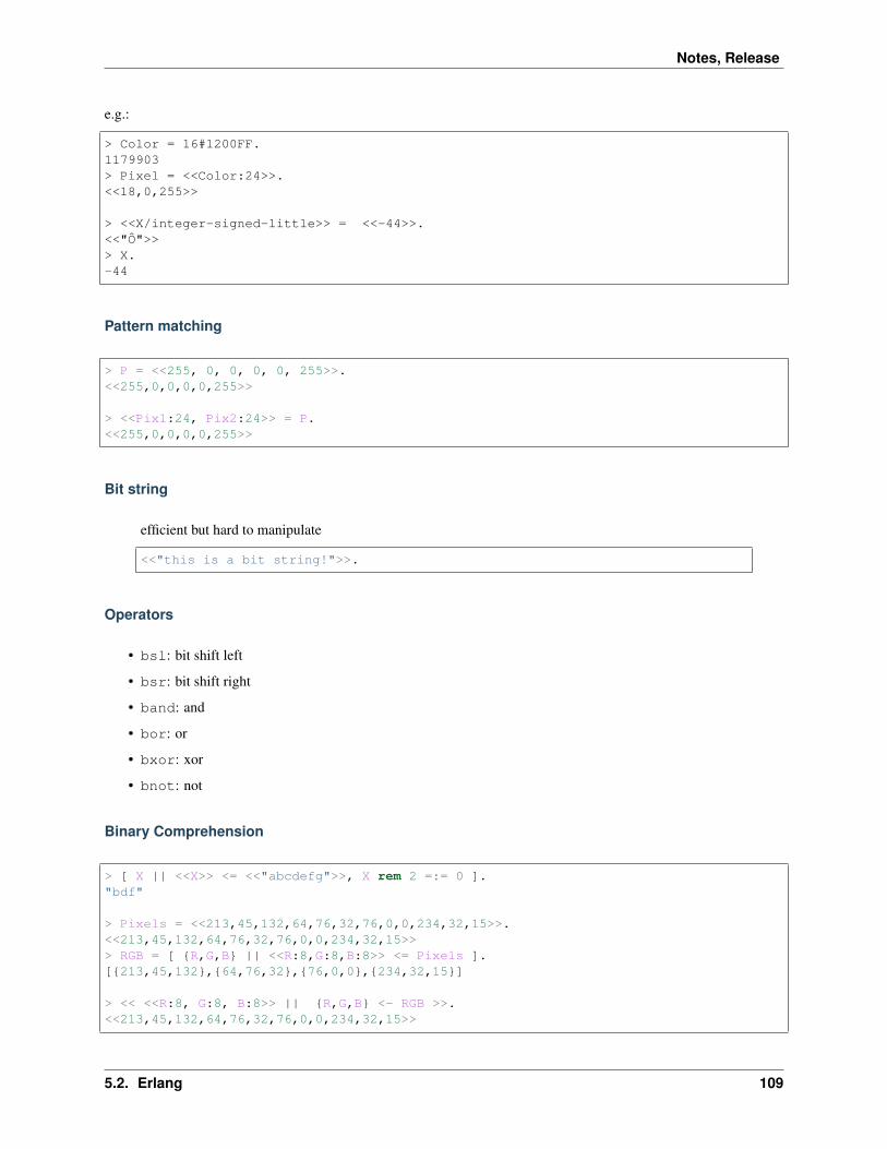
Notes, Release

e.g.:

> Color = 16#1200FF.1179903> Pixel = <<Color:24>>.<<18,0,255>>

> <<X/integer-signed-little>> = <<-44>>.<<"Ô">>> X.-44

Pattern matching

> P = <<255, 0, 0, 0, 0, 255>>.<<255,0,0,0,0,255>>

> <<Pix1:24, Pix2:24>> = P.<<255,0,0,0,0,255>>

Bit string

efficient but hard to manipulate

<<"this is a bit string!">>.

Operators

• bsl: bit shift left

• bsr: bit shift right

• band: and

• bor: or

• bxor: xor

• bnot: not

Binary Comprehension

> [ X || <<X>> <= <<"abcdefg">>, X rem 2 =:= 0 ]."bdf"

> Pixels = <<213,45,132,64,76,32,76,0,0,234,32,15>>.<<213,45,132,64,76,32,76,0,0,234,32,15>>> RGB = [ R,G,B || <<R:8,G:8,B:8>> <= Pixels ].[213,45,132,64,76,32,76,0,0,234,32,15]

> << <<R:8, G:8, B:8>> || R,G,B <- RGB >>.<<213,45,132,64,76,32,76,0,0,234,32,15>>

5.2. Erlang 109

Notes, Release

5.2.2 Erlang Module

call a function from module Module:Function(Args).

> lists:seq(1, 10).[1,2,3,4,5,6,7,8,9,10]

Declaration

Attribute

Sytax

-Name(Attribute).

Required attribute

-module(Name).

Name is an atom

Export functions

-export([Function1/Arity, Function2/Arity, ..., FunctionN/Arity]).

Arity How many arg can be passed to the function.

Different function can share same name: add(X, Y) and add(X, Y, Z). They will carrydiffrent arity: add/2 and add/3.

Import functions

Invoking an external function do not require imported, just do this like we do in the shell:

-module(name)...g -> 10 * other_module:some_f(100).

But this maybe get too verbose when we using lots of external functions.

So we have -import directive for removing the module prefix during invoking.

-import(Module, [Function/Arity, ...]).

-import(io, [format/1])....g - > format(...). % not io:format


Notes, Release

Macro

similar to C’s Macro. They will be replace before compiling.

-define(MACRO, value).

Use as ?MACRO inside code.

e.g.:

-define(sub(X, Y), X - Y).

Function

Sytax

Name(Args) -> Body.

Name an atom

Body one or more erlang expressions

Return The value of last expression

e.g:

add(X, Y) ->X + Y.

hello() ->io:format("Hello World!~n").

Compile the code

• $ erlc file.erl

• In shell, c(module)

• In shell or module, compile:file(FileName)

Define compiling flags in module

e.g.: -compile([debug_info, export_all, ...]).

Note: export_all make native compiler conservative. But using export_all with normal BEAM vm is almostnot affected.

Ref: https://stackoverflow.com/questions/6964392/speed-comparison-with-project-euler-c-vs-python-vs-erlang-vs-haskell#answer-6967420

5.2. Erlang 111

https://stackoverflow.com/questions/6964392/speed-comparison-with-project-euler-c-vs-python-vs-erlang-vs-haskell#answer-6967420

https://stackoverflow.com/questions/6964392/speed-comparison-with-project-euler-c-vs-python-vs-erlang-vs-haskell#answer-6967420

Notes, Release

Compile into native code

There is two way to deal with it.

• hipe:c(Module, OptionList).

• c(Module, native).

More about module

module_info/0

> test:module_info().[module,test,exports,[add,2,module_info,0,module_info,1],attributes,[vsn,[146299772997766369192496377694713339991]],compile,[options,[native],

version,"6.0",time,2015,7,12,15,5,54,source,"/tmp/test.erl"],

native,true,md5,<<179,5,110,53,195,122,250,63,30,245,110,140,79,

121,143,254>>]

module_info/1

> test:module_info(exports).[add,2,module_info,0,module_info,1]

vns

This is an auto generated version for your code. It’s used for hot-loading.

> hd(test:module_info(attributes)).vsn,[146299772997766369192496377694713339991]

It can be set manually.

-vsn(VersionNumber).

Other directives

• -author(Name)

• -date(Date)

• -behavior(Behavior)

• -record(Name, Field)


Notes, Release

Documenting Modules

Erlang includes doc system called EDoc.

Sample module called hello.erl:

%% @author Iblis Lin <[email protected]> [https://github.com/iblis17]%% @doc The features of this module.%% @version

- module(name)....

Then we can build it via shell:

1> edoc:files(["hello.erl"], [dir, "docs"]).ok

Now we will get some html files in docs folder.

5.2.3 Erlang Function

Basic

1> F = fun(X) ->math:sqrt(X) * 10

end.

2> G = fun(X) ->Y = math:sqrt(X),10 * Y

end.

Bind function from module

Assume we have a function f/1 in the module hello. If we want to bind hello:f to variable:

1> F = fun hello:f/1.2> F(...).

Pattern Matching

Function Clause

Sample: replace if

def g(gender, name):if gender == 'male':

print('Hello, Mr. '.format(name))elif:

print('Hello, Mrs. '.format(name))else:

print('Hello, '.format(name))

5.2. Erlang 113

Notes, Release

In Erlang:

g(male, Name) ->io:format("Hello, Mr. ~s", [Name]);

g(female, Name) ->io:format("Hello, Mrs. ~s", [Name]);

g(_, Name) ->io.format("Hello, ~s", [Name]).

Guards

Addictional clause to check vars. Let us check the content of argument, not only shape/position.

It’s indicated by when.

It can use only a small set of builtin functions to guarantee there is’nt no side effect.

Multiple conditions:

• , (commas): like and, e.g.: when X >= 60, X =< 100 -> ...

• ; (semicolons): like or

is_pass(X)when X >= 60, X =< 100 ->

true.is_pass(_) ->

false.

> module:is_pass(80).true

> module:is_pass(a).true%% what happend ?!

case expression

It let you move pattern matching inside function.

It’s similar to case but without pattern matching.

5.2.4 Data Structures

Record

• Just like namedtuple in Python.

• In erlang shell, rr(module) to load _records_.

• It’s an syntax sugar for compiler


Notes, Release

5.2.5 Concurrent

receive

receivePattern1 -> value;Pattern2 -> value

after Time ->value

end.

Note: Time is in millionseconds, but can be atom infinity.

Link

> “I am going to die if my partner dies.”

Here is a race condiction:

link(spawn(...)).

It’s possible that the process crash before the link established. So, please use:

spawn_link(...).

Trap

Turn a process into system process:

process_flag(trap_exit, true).

And get exception via receive expression, e.g.:

spawn_link(fun() -> timer:sleep(1000), exit(magic) end), receive X -> X end.

%% will get 'EXIT',<0.134.0>,magic.

The kill signal cannot be trapped:

> process_flag(trap_exit, true).false> exit(self(), kill).

** exception exit: killed

Note: Because the kill signal cannot be trapped, so the it will be changed to killed when other process receivethe message.

Monitor

It’s special type of link with

5.2. Erlang 115

Notes, Release

• unidirection

• can be stacked

erlang:monitor(process, Pid).

Note the potential race condiction in following code:

erlang:monitor(process, spawn(fun() -> ok end)).

So here is an atomic function:

spawn_monitor(fun() -> ok end).

Demonitor:

erlang:demonitor(Ref).erlang:demonitor(Ref, [flush, info]).

Naming Porcess

• register(atom, Pid)

And just send via atom:

> atom ! self(), hello<pid>, hello

5.2.6 Designing a Concurrent Application

Origin: http://learnyousomeerlang.com/designing-a-concurrent-application

• “A reminder app”

Requirement

Task:

name deadline

Operation:

• Cancel event by name.

• Task deadline alert.

Component

• Task Server

• Client

• Task process


http://learnyousomeerlang.com/designing-a-concurrent-application

Notes, Release

Protocol

• client monitor server

• server monitor client, also

> client can live without server, and vice versa.

5.2.7 Finite State Machine

• elements: (State), Event, and Data ()

Event State A Event foo (with Data X) State B

Simple cat FSM:

1 -module(cat_fsm).2

3 -compile(export_all).4

5 -behaviour(gen_fsm).6

7

8 %%%%%%%%%%%%%%%%%%%%%%%%%%%%%%%%%%%%%%%%%%%%%%%%%%9 %%% public api

10 %%%%%%%%%%%%%%%%%%%%%%%%%%%%%%%%%%%%%%%%%%%%%%%%%%11

12 start() ->13 ok, Pid = gen_fsm:start(?MODULE, [], []),14 Pid.15

16

17 stop(Pid) ->18 gen_fsm:stop(Pid).19

20

21 poke(Pid) ->22 gen_fsm:sync_send_event(Pid, poke, 5000).23

24

25 %%%%%%%%%%%%%%%%%%%%%%%%%%%%%%%%%%%%%%%%%%%%%%%%%%26 %%% export for generic fsm framework27 %%%%%%%%%%%%%%%%%%%%%%%%%%%%%%%%%%%%%%%%%%%%%%%%%%28

29 init(_) ->30 ok, meow, data, 5000.31

32

33 terminate(_, _, _) ->34 ok.35

36

37 meow(timeout, _Data) ->38 io:format("meow~n"),39 next_state, meow, [], 5000;40

41 meow(Unknown, _Data) ->42 io:format("meow ~p~n", [Unknown]),43 next_state, meow, [], 5000.

5.2. Erlang 117

Notes, Release

44

45

46 meow(poke, _From, _Data) ->47 reply, jump, meow, [], 5000.48

49

50 code_change(_OldVer, _State, _Data, _Extra) ->51 %% do nothing52 ok, meow, [].

5.2.8 stdlib

Eunit

• put testing code in test dir.

• include the eunit header file.

• naming:

– ... _test(): single test case

– ... _test_(): test cases generator, return a list of testing cases function.

5.3 Python

5.3.1 Basic

Builtin Functions

print

>>> print('\v'.join(map(str,range(10))))0123456789

>>> print('\v'.join(map(str, range(10, 20))))10

1112

131415

1617


Notes, Release

1819

Exception

Handy args

>>> e = Exception('reason', 'detail')>>> e.args('reason', 'detail')

property decorator

How dose it work? It return a Descriptor Object.

Data Descriptor An object defines both __get__() and __set__()

Non-data Descriptor An object only defines __get__()

Make read-only data descriptor: make __set__ raise AttributeError.

Attribute Lookup

a.x

Order:

1. Data descriptor

2. a.__dict__['x']

3. type(a).__dict__['x']

4. Non-data descriptor

Ref:

• http://stackoverflow.com/questions/17330160/how-does-the-property-decorator-work

• https://docs.python.org/3.6/howto/descriptor.html

Standard Library

multiproccessing.pool

map, imap variants map chunck_size iterable iterable early evaluated lazy

stdlib (3.6) producer & consumer

Ref: https://stackoverflow.com/questions/5318936/python-multiprocessing-pool-lazy-iteration

5.3. Python 119

http://stackoverflow.com/questions/17330160/how-does-the-property-decorator-work

https://docs.python.org/3.6/howto/descriptor.html

https://stackoverflow.com/questions/5318936/python-multiprocessing-pool-lazy-iteration

Notes, Release

5.3.2 Web

Django

Deployment

• heroku

• pythonanywhere

5.3.3 Project

5.4 R Language

• Intro

5.5 Lua

5.5.1 Lua basic

Terms

Chunk a sequence of statements

Quote

> 'hello' == "hello" -- true

Function

function t(args)...

end

Assignment

-- ugly, but valid> a = 1 b = a * 2

Commend Line

-l <chunk>

Execute chunk


http://nbviewer.jupyter.org/github/iblis17/notes/blob/master/lang/r/intro.ipynb

Notes, Release

$ cat c1.luaa = 100

$ cat c2.luab = 3

$ cat c3.luaprint(a * 3)

$ lua -l c1 -l c2 c3300

This will execute c1 and c2 first.

5.6 JavaScript

5.6.1 ECMAScript 6

Destructuring

Looks like var unpacking in python, but more powerful. It can handle object.

Ref

• https://github.com/lukehoban/es6features#destructuring

Fetch API

fetch('https://path/toapi/url').then(function(res)console.log('aaaaa'); return res).then(function(res)console.log(res))

Ref

• https://developer.mozilla.org/en-US/docs/Web/API/Fetch_API

• https://developer.mozilla.org/en-US/docs/Web/API/GlobalFetch/fetch

5.6.2 Airbnb JS Coding Style Guide

let

If we cannot use const, use let instead of var. let is block-scope.

Ref: https://github.com/airbnb/javascript#references--disallow-var

5.6. JavaScript 121

https://github.com/lukehoban/es6features#destructuring

https://developer.mozilla.org/en-US/docs/Web/API/Fetch_API

https://developer.mozilla.org/en-US/docs/Web/API/GlobalFetch/fetch

https://github.com/airbnb/javascript#references--disallow-var

Notes, Release

5.7 Julia

5.7.1 Basic

Blog

some reading about julia blog

AOT

ref: https://juliacomputing.com/blog/2016/02/09/static-julia.html

• blocker of static analysis: eval, macro, generated

Calling C Functions

• Julia can call a c function without glue code

• ccall()

• Function in shared library only

Code Generation

julia> 𝜆(l) = l ^ 2𝜆 (generic function with 1 method)

julia> code_native(𝜆, (Float64,)).text

Filename: REPL[3]pushq %rbpmovq %rsp, %rbp

Source line: 1vmulsd %xmm0, %xmm0, %xmm0popq %rbpretqnopw (%rax,%rax)

julia> code_native(𝜆, (Int,)).text

Filename: REPL[3]pushq %rbpmovq %rsp, %rbp

Source line: 1imulq %rdi, %rdimovq %rdi, %raxpopq %rbpretqnopl (%rax)


https://juliacomputing.com/blog/2016/02/09/static-julia.html

Notes, Release

Flow Control

if

if...

elseif...

end

for

for i = [1, 2, 3]println(i)

end

for i in [1, 2, 3]println(i)

end

for i in 1:5println(i^2)

end

for i in Dict("foo" => 1, "bar" => 2)println(i)

end

for (k, v) in Dict("foo" => 1, "bar" => 2)println(k, ": ", v)

end

while

while ......

end

try

try...

catch e...

end

Function

Function will return the last expression. return is still allow.

5.7. Julia 123

Notes, Release

julia> function 𝜆(x, y)x + y

end𝜆 (generic function with 1 method)

julia> 𝜆(2, 5)7

Compact declaration:

julia> f(x, y) = x ^ yf (generic function with 1 method)

Return tuple:

julia> 𝜆(x, y) = x + y, x - y𝜆 (generic function with 1 method)

julia> 𝜆(2, 3)(5,-1)

Arbitrary positional arguments:

function 𝜆(args...)println(args) # tuple

end

Function call unpacking:

𝜆([1, 2, 3]...)

Default arguments:

function 𝜆(x, y=2, z=10)x ^ y + z

end

Keyword only arguments:

function 𝜆(x; y=2, z=10)x ^ y + z

end

𝜆(10; y=3)# or𝜆(10; :y=>3)

Keyword args function call:

𝜆(; y=2, z=10)

𝜆(; :y=>2, :z=>10)

𝜆(; (:y,2), (:z, 10))


Notes, Release

Functions

built-in

typeof:

julia> typeof(:foo)Symbol

in:

julia> a2×3 ArrayInt64,2:1 2 34 5 6

julia> 1 atrue

julia> 1 afalse

length and size:

julia> a2×3 ArrayInt64,2:1 2 34 5 6

julia> length(a)6

julia> size(a)(2, 3)

Anonymous Function

x -> x + 42

Multiple-Dispatch

julia> function 𝜆(a::Int, b::Int)a + b


julia> function 𝜆(a::Float, b::FloatFloat16 Float32 Float64julia> function 𝜆(a::Float64, b::Float64)

a * bend

𝜆 (generic function with 2 methods)

5.7. Julia 125

Notes, Release

Valc

const c type Valc

Multiple dispatch c run-time

e.g.:

julia> f(::TypeValtrue) = 42f (generic function with 1 methods)

julia> f(Valtrue)42

idea: pattern matching

Meta Programming

Generated Functions

• special macro @generated

• return a quoted expression

• caller type code generation.

e.g.:

@generated function foo(x)# x denote type here# will show Int, Float64, String, ... etcprintln(x) # invoke at copmile, and only *once*return :(x * x)

• loop unroll ( type )

Macros in Base

• Base.@pure

• Base.@nexprs

• Base.@_inline_meta

Module

• each module has its own global scope

Performance Tips

Ref: https://docs.julialang.org/en/latest/manual/performance-tips/


https://docs.julialang.org/en/latest/manual/performance-tips/

Notes, Release

Avoid global variables

global var type compiler const optimize

Benchmark and Memory allocation

• builtin: @time

• BenchmarkTools

Avoid constainer with abstract type parameters

e.g: 𝑎 = 𝑅𝑒𝑎𝑙[] array Real , Real element size , a array of pointer points to Real object. Real objectallocation

Scope of Variables

Global Scope

• module

• baremodule

• REPL

global scope

Soft Local Scope parent scope, local keyword

• for

• while

• comprehensions

• try

• let

Hard Local Scope parent scope, assignement or local keyword

• function

• struct

• macro

No new scope

• begin

• if

5.7. Julia 127

Notes, Release

Standard Lib

Collections

Array

• fill("", 10): like [""] * 10 in python.

• mapslices(f, A, dims): Array slice f dims : slice

f 2× 3× 4× 5 dim = [3, 4] [i, j, :, :]

• foreach: map outcome

Iterations

An iterable object interface:

• start()

• done()

• next()

See also: http://docs.julialang.org/en/latest/manual/interfaces.html#man-interface-iteration-1

Date

julia> collect(Date("2017-1-1"):Date("2017-2-1"))32-element ArrayDate,1:2017-01-012017-01-022017-01-032017-01-042017-01-052017-01-062017-01-072017-01-082017-01-092017-01-102017-01-112017-01-122017-01-132017-01-142017-01-152017-01-162017-01-172017-01-182017-01-192017-01-202017-01-212017-01-222017-01-232017-01-242017-01-252017-01-262017-01-27


http://docs.julialang.org/en/latest/manual/interfaces.html#man-interface-iteration-1

Notes, Release

2017-01-282017-01-292017-01-302017-01-312017-02-01

• TimeDate with StepRange:

DateTime(2017, 1, 1, 8, 0, 0):Dates.Hour(2):DateTime(2017, 1, 1, 20, 0, 0)

Filesystem

like python’s __file__:

dirname(@__FILE__)

• 0.6+ has @__DIR__

Network

• download

OS Utils

• withenv: temporary change env var(s):

withenv("PWD" => nothing) do # ``nothing`` can delete the varprintln(ENV["PWD"])

end

Broadcast

• broadcast_getindex: getindex ( broadcast )

Base.Random

• uuid1: time-based UUID

• uuid4

Type

• optional static type

5.7. Julia 129

Notes, Release

Float

• IEEE 754

• Inf:

julia> Inf > NaNfalse

• -Inf

• NaN:

julia> NaN == NaNfalse

julia> NaN != NaNtrue

# Notejulia> [1 NaN] == [1 NaN]false

functions

• isequal(x, y):

julia> isequal(1.0000000000000000000000001, 1.0000000000000001)true

# Notejulia> isequal(NaN, NaN)ture# diff from ``NaN == NaN``

julia> isequal([1 NaN], [1 NaN])true

• isnan(x)

Array

a = [1, 2, 3]

a[1] # 1a[end] # 3

with type:

a = Float64[1, 2, 3]a = Int[1, 2, 3]


Notes, Release

Matrix

a = [1 2 3]

a = [1 2 3; 4 5 6]

with type:

a = Int[1 2 3]

Range

julia> [1:10]1-element ArrayUnitRangeInt64,1:1:10

julia> [1:10;]10-element ArrayInt64,1:12345678910

julia> [1:3:20;]7-element ArrayInt64,1:14710131619

Dict

Dict()

d = Dict("foo" => 1, "bar" => 2)

keys(d)

values(d)

("foo" => 1) d

haskey(d, "foo")

5.7. Julia 131

Notes, Release

Pair

p = "foo" => 1p[1] == "foo"p[2] == 1

typeof

Int64:

julia> typeof(42)Int64

julia> typeof(Int64)DataType

julia> typeof(42)Int64

julia> supertype(Int64)Signed

julia> supertype(Signed)Integer

julia> supertype(Integer)Real

julia> supertype(Real)Number

julia> supertype(Number)Any

julia> supertype(Any)Any

String:

julia> typeof("test")String

julia> supertype(String)AbstractString

julia> supertype(AbstractString)Any

Class

type Catname::Stringage::Int

end


Notes, Release

Cat("meow", Int)

• note that :: is type annotation.

• a::C can read as “a is an instance of C”.

• concrete type cannot have subtype:

struct S...

end

• struct are immutable

Type Assertion

Assertion

(1 + 2)::Int

(1 + 2)::Float64 # error

Type Declaration

• @code_typed & @code_lowerd check type stability

• ResultTypes.jl backtrace

Annotation (Declaration)

julia> function 𝜆()x::Int8 = 10x

end𝜆 (generic function with 2 methods)

julia> 𝜆()10

julia> typeof(𝜆())Int8

only allowed in non-global scope:

function f()x::Int = 4y::Float64 = 3.14z::Float16 = 2

x, y, zend

5.7. Julia 133

https://github.com/iamed2/ResultTypes.jl

Notes, Release

julia> f()(4, 3.14, Float16(2.0))

Return Type Annotation

On function definition:

julia> function 𝜆()::Int6442.0


julia> 𝜆()42 # alway be converted to Int64

“This method must return a T”:

function f()::Int42

end

It can be parametrize as well:

function f(v::VectorT)::T where T <: Real...

end

It can be expression, e.g. using the return value of a function call:

function f(v::VectorT)::promote_type(T) where T <: Real...

end

It can be depend on argument:

function f(x)::eltype(x)...

end

Abstract Types

Declaration:

abstract type MyType endabstract type MyType <: MySupperType end

• <: can read as “is subtype of”:

julia> Int64 <: Inttrue

julia> Int64 <: Realtrue


Notes, Release

julia> Int64 <: Float64false

• function will be compiled on demand with concrete type:

f(x) = x * 2

means:

f(x::Any) = x * 2

If we invoke f(1), the function f(x::Int) = ... will be compiled.

Parametric Types

• like template in C++

• Generic programming: https://en.wikipedia.org/wiki/Generic_programming

Parametric Type

struct PointTx :: Ty :: T

end

concrete type, e.g. PointFloat64, PointString ...

Point id type object, Point... :

julia> PointFloat64 <: Pointtrue

julia> PointAbstractString <: Pointtrue

julia> PointAbstractVectorInt <: Pointtrue

concrete type :

julia> PointFloat64 <: PointStringfalse

Real Float64 :

julia> PointFloat64 <: PointRealfalse

Julia type parameter invariant invariant type parameter type Real vs Float64 invariant juliaPointFloat64 , 64-bits

covariant type :

PointFloat64 <: Point<:Realtrue

5.7. Julia 135

https://en.wikipedia.org/wiki/Generic_programming

Notes, Release

contravariant:

PointReal <: Point>:Float64true

function argument PointT, T Real subtype :

# in julia both 0.5 and 0.6function fT<:Real(x::PointT)

# ...end

# in julia 0.6function f(x::Point<:Real)

# ...end

function f(x::PointT) where T<:Real# ...

end

Parametric Method

julia 0.5:

same_typeT(x::T, y::T) = true

# abstract typesame_typeT<:AbsType(x::T, y::T) = true

0.6:

same_type(x::T, y::T) where T = true

# abstract typesame_type(x::T, y::T) where T<:AbsType = true

Tuple Type

https://docs.julialang.org/en/latest/manual/types.html#Tuple-Types-1

NTuple Tuple type compact representation:

julia> NTuple3, Int TupleInt64,Int64,Int64

julia> NTuple6, Int NTuple6,Int64

• covariant

• Vararg Tuple covariant

julia> VarargInt, 3 <: VarargInteger, 3true


https://docs.julialang.org/en/latest/manual/types.html#Tuple-Types-1

CHAPTER 6

Math

6.1 Calculus

6.1.1 Prepartion

Equation

• graphically

• analytically

• numerically

Intercepts (𝑎, 0) or (0, 𝑏)

• (𝑎, 0) x-intercept

• (0, 𝑏) y-intercept

• ...etc

intercept ,

Transformation of Functions

𝑦 = 𝑓(𝑥)

• 𝑦 = 𝑓(𝑥+ 𝑐)

• 𝑦 = 𝑓(𝑥) + 𝑐

• Reflection x-axis 𝑦 = −𝑓(𝑥)

• Reflection y-axis 𝑦 = 𝑓(−𝑥)

• Reflection 𝑦 = −𝑓(−𝑥)

Algebraic Functions function, algebraic operations

137

Notes, Release

Algebraic Operations

Transcendental Functions Algebraic Functions,

Composite Function

(𝑓 ∘ 𝑔) = 𝑓(𝑔(𝑥))

Elementary Functions

One variable composite with finite number of

• arithmetic operation: + − ×÷

• exponentials

• logarithms

• constants

6.1.2 Limits

1.2 Finding limits

𝑓

6.1.3 Total Derivative

Let 𝑓(𝑥, 𝑦) = 𝑥𝑦

𝑥, 𝑦 independent

𝑑𝑓

𝑑𝑥= 𝑦

𝑑𝑓

𝑑𝑦= 𝑥

𝑥, 𝑦 dependent 𝑦 = 𝑥

𝑓(𝑥, 𝑦) = 𝑥𝑦 = 𝑥2

𝑑𝑓

𝑑𝑥= 2𝑥

𝑑𝑓𝑑𝑥 chain rule

𝑑𝑓

𝑑𝑥=𝜕𝑓

𝜕𝑥+𝜕𝑓

𝜕𝑦

𝑑𝑦

𝑑𝑥

=𝜕𝑓

𝜕𝑥+𝜕𝑓

𝜕𝑦× 1

=𝜕𝑓

𝜕𝑥+ 𝑥𝑡𝑖𝑚𝑒𝑠1

= 𝑦 + 𝑥

= 2𝑥

dependent chain rule chain rule general form independent chain rule 0

138 Chapter 6. Math

Notes, Release

Ref

• https://en.wikipedia.org/wiki/Total_derivative

6.2 Differential Equations

6.3 Linear Algebra

6.3.1 Linear Transform

Ref: Chap 6

function map vector space: 𝑉 and 𝑊 .

𝑇 : 𝑉 →𝑊

• V T domain

• W T codomain

𝑇 () =

• image

• output set: preimage of

Definition

𝑉, 𝑊 vector space

𝑇 : 𝑉 →𝑊

1. 𝑇 (+ ) = 𝑇 () + 𝑇 (𝑡)

2. 𝑇 (𝑐) = 𝑐𝑇 ()

(P.294)

Counterexample

sin function Linear Transform

sin((𝜋

2) + (

𝜋

3)) = sin(

𝜋

2) + sin(

𝜋

3)

Matrix Form

𝑇 () = 𝐴

𝐴 shape (3, 2)

𝑇 : 𝑅2 → 𝑅3

image 𝐴

6.2. Differential Equations 139

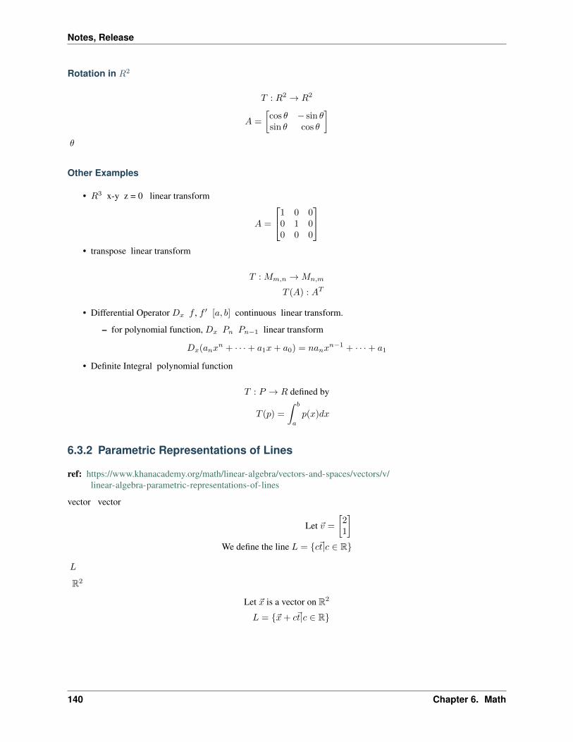
https://en.wikipedia.org/wiki/Total_derivative

Notes, Release

Rotation in 𝑅2

𝑇 : 𝑅2 → 𝑅2

𝐴 =

[cos 𝜃 − sin 𝜃sin 𝜃 cos 𝜃

]𝜃

Other Examples

• 𝑅3 x-y z = 0 linear transform

𝐴 =

⎡⎣1 0 00 1 00 0 0

⎤⎦• transpose linear transform

𝑇 : 𝑀𝑚,𝑛 →𝑀𝑛,𝑚

𝑇 (𝐴) : 𝐴𝑇

• Differential Operator 𝐷𝑥 𝑓 , 𝑓 ′ [𝑎, 𝑏] continuous linear transform.

– for polynomial function, 𝐷𝑥 𝑃𝑛 𝑃𝑛−1 linear transform

𝐷𝑥(𝑎𝑛𝑥𝑛 + · · ·+ 𝑎1𝑥+ 𝑎0) = 𝑛𝑎𝑛𝑥

𝑛−1 + · · ·+ 𝑎1

• Definite Integral polynomial function

𝑇 : 𝑃 → 𝑅 defined by

𝑇 (𝑝) =

∫ 𝑏

𝑎

𝑝(𝑥)𝑑𝑥

6.3.2 Parametric Representations of Lines

ref: https://www.khanacademy.org/math/linear-algebra/vectors-and-spaces/vectors/v/linear-algebra-parametric-representations-of-lines

vector vector

Let =

[21

]We define the line 𝐿 = 𝑐|𝑐 ∈ R

𝐿

R2

Let is a vector on R2

𝐿 = + 𝑐|𝑐 ∈ R

140 Chapter 6. Math

https://www.khanacademy.org/math/linear-algebra/vectors-and-spaces/vectors/v/linear-algebra-parametric-representations-of-lines

https://www.khanacademy.org/math/linear-algebra/vectors-and-spaces/vectors/v/linear-algebra-parametric-representations-of-lines

Notes, Release

Parametric Representations

,

𝐿 = + 𝑐(𝑎− )|𝑐 ∈ R (6.1)or(6.2)

𝐿 = 𝑏+ 𝑐(𝑎− )|𝑐 ∈ R(6.3)

6.4 Probability

6.4.1 Probability Axioms

Terms

𝑃 (𝐴) = 0.6

Input Event

Domain Event Space , Event

Output 0 - 1

Event Set, 0 or more samples

Sample outcome

Sample Space outcome Set 𝑆, 𝑃 (𝑆) = 1

Event Space sample(s) Event sample(s) Event Space

e.g. Sample Space 𝑆 = 𝑓𝑜𝑜, 𝑏𝑎𝑟, 𝑏𝑎𝑧 Event 𝑓𝑜𝑜, 𝑏𝑎𝑧 Event Space 8 Event 23 = 8 sample boolen

Axioms

1.

∀ Event 𝐴, 𝑃 (𝐴) ≥ 0

2.

𝑃 (𝑆) = 1

3.

Event 𝐴1, 𝐴2, . . . Mutual Exclude, then𝑃 (𝐴1 ∪𝐴2 ∪ . . . ) = 𝑃 (𝐴1) + 𝑃 (𝐴2) + . . .

6.4. Probability 141

Notes, Release

Properties

1. from axiom 3

𝐸 = 𝑜1, 𝑜2, . . . , 𝑛 (6.4)= 𝑜1 ∪ 𝑜2 ∪ · · · ∪ 𝑜𝑛(6.5)

𝑃 (𝐸) = 𝑃 (𝑜1) + 𝑃 (𝑜2) + · · ·+ 𝑃 (𝑜𝑛)(6.6)(6.7)

2.

𝑃 (𝜑) = 0

∵ 𝑆 ∩ 𝜑 = 𝜑 ∴ 𝑆, 𝜑 is Mutual Exclude

3.

𝑃 (𝐴) = 1− 𝑃 (𝐴𝑐)

4.

𝑃 (𝐴) = 𝑃 (𝐴−𝐵) + 𝑃 (𝐴 ∩𝐵)

5.

𝑃 (𝐴 ∪𝐵) = 𝑃 (𝐴) + 𝑃 (𝐵)− 𝑃 (𝐴 ∩𝐵)

6. 𝑆 𝐴

𝐶1, 𝐶2, . . . , 𝐶𝑛 Mutual Exclude, and𝐶2 ∪ 𝐶2 ∪ · · · ∪ 𝐶𝑛 = 𝑆

∀ Event 𝐴𝑃 (𝐴) = 𝑃 (𝐴 ∩ 𝐶1) + 𝑃 (𝐴 ∩ 𝐶2) + · · ·+ 𝑃 (𝐴 ∩ 𝐶𝑛)

7.

𝐴 ⊂ 𝐵, then 𝑃 (𝐴) < 𝑃 (𝐵)

8. Boole’s 𝐴𝑖

𝑃 (∪𝑛𝑖=1𝐴𝑖) ≤𝑛∑𝑖=1

𝑃 (𝐴𝑖)

9. Bonferroni’s 𝐴𝑖

𝑃 (∩𝑛𝑖=1𝐴𝑖) ≥ 1−𝑛∑𝑖=1

𝑃 (𝐴𝑐𝑖 )

142 Chapter 6. Math

Notes, Release

6.4.2 Conditional Probability

Sample Space

𝑃 of 𝑜𝑖 given 𝑌 :

𝑌 = 𝑜1, . . . , 𝑜𝑛 (6.8)

𝑃 (𝑜𝑖|𝑌 ) =𝑃 (𝑜𝑖)

𝑃 (𝑜1) + · · ·+ 𝑃 (𝑜𝑛)(6.9)

=𝑃 (𝑜𝑖)

𝑃 (𝑌 )(6.10)

𝑃 of 𝑋 given 𝑌 :

𝑋 = 𝑜1, 𝑜2, 𝑞1, 𝑞2 (6.11)𝑌 = 𝑜1, 𝑜2, 𝑜3(6.12)

𝑃 (𝑋|𝑌 ) = 𝑃 (𝑜1|𝑌 ) + 𝑃 (𝑜2|𝑌 )(6.13)

=𝑃 (𝑋 ∩ 𝑌 )

𝑃 (𝑌 )(6.14)

𝑃 (𝑞1|𝑌 ) = 0(6.15)

Product Rule

𝑃 (𝑋 ∩ 𝑌 ) = 𝑃 (𝑋|𝑌 )𝑃 (𝑌 ) (6.16)= 𝑃 (𝑌 |𝑋)𝑃 (𝑋)(6.17)

Properties

1.

𝑃 (𝑋|𝑌 ) =𝑃 (𝑋 ∩ 𝑌 )

𝑃 (𝑌 )≥ 0

2.

𝑃 (𝑌 |𝑌 ) =𝑃 (𝑌 ∩ 𝑌 )

𝑃 (𝑌 )= 1

3. 𝐴,𝐵 Mutual Exclude

𝑃 (𝐴 ∪𝐵|𝑌 ) =𝑃 (𝐴)

𝑃 (𝑌 )+𝑃 (𝐵)

𝑃 (𝑌 )= 𝑃 (𝐴|𝑌 ) + 𝑃 (𝐵|𝑌 )

Total Probability

Properties (6)

𝑃 (𝐴) = 𝑃 (𝐴 ∩ 𝐶1) + 𝑃 (𝐴 ∩ 𝐶2) + · · ·+ 𝑃 (𝐴 ∩ 𝐶𝑛) (6.18)= 𝑃 (𝐴|𝐶1)𝑃 (𝐶1) + 𝑃 (𝐴|𝐶2)𝑃 (𝐶2) + · · ·+ 𝑃 (𝐴|𝐶𝑛)𝑃 (𝐶𝑛)(6.19)

6.4. Probability 143

Notes, Release

Bayes’ Rule

𝑃 (𝐶𝑗 |𝐴) =𝑃 (𝐴|𝐶𝑗)𝑃 (𝐶𝑗)

𝑃 (𝐴|𝐶1)𝑃 (𝐶1) + · · ·+ 𝑃 (𝐴|𝐶𝑛)𝑃 (𝐶𝑛)

proof:

𝑃 (𝐶𝑗 |𝐴) =𝑃 (𝐶𝑗 ∩𝐴)

𝑃 (𝐴)(6.20)

=𝑃 (𝐴 ∩ 𝐶𝑗)𝑃 (𝐴)

(6.21)

=𝑃 (𝐴|𝐶𝑗)𝑃 (𝐶𝑗)

𝑃 (𝐴)(6.22)

By Total Probability =𝑃 (𝐴|𝐶𝑗)𝑃 (𝐶𝑗)∑𝑛𝑖=1 𝑃 (𝐴|𝐶𝑖)𝑃 (𝐶𝑖)

(6.23)

6.5 Statistic

6.5.1 Autocorrelation

serial correlation

Specific form: - unit root processes - trend stationary processes - autoregressive processes - moving average processes

Def

random process autocorrelation Pearson Correlation

𝑅(𝑠, 𝑡) =𝐸[(𝑋𝑡 − 𝜇𝑡)(𝑋𝑠 − 𝜇𝑠)]

𝜎𝑡𝜎𝑠

time series autocorrelation function (ACF)

𝐶𝑜𝑟𝑟(𝑦𝑡, 𝑦𝑡−𝑘)

𝑘 lag

Partial Autocorrelation Function (PACF)

• conditional correlation (?)

• pacf in StatsBase

Reference

• http://juliastats.github.io/StatsBase.jl/stable/signalcorr.html#StatsBase.autocor

• https://en.wikipedia.org/wiki/Autocorrelation

• PACF: https://onlinecourses.science.psu.edu/stat510/node/62

• https://en.wikipedia.org/wiki/Partial_correlation

144 Chapter 6. Math

http://juliastats.github.io/StatsBase.jl/stable/signalcorr.html#StatsBase.autocor

https://en.wikipedia.org/wiki/Autocorrelation

https://onlinecourses.science.psu.edu/stat510/node/62

https://en.wikipedia.org/wiki/Partial_correlation

Notes, Release

6.5.2 Autoregressive Model

Def

AR(1)

𝑦𝑡 = 𝛽0 + 𝛽1𝑦𝑡−1 + 𝜖𝑡

order of autoregression:

AR(k)

𝑦𝑡 = 𝛽0 + 𝛽1𝑦𝑡− 1 + · · ·+ 𝛽𝑘𝑦𝑡−𝑘 + 𝜖𝑡

Examples

AR(1) plot

using Gadfly, MarketDataplot(x=cl.values[1:end-1], y=cl.values[2:end])

linear model

Reference

• https://onlinecourses.science.psu.edu/stat501/node/358

6.5.3 Durbin-Waston Test

residual (prediction error) Autocorrelation

Def

𝑑 =

∑𝑇𝑡=2(𝑒𝑡 − 𝑒𝑡−1)2∑𝑇

𝑡=1 𝑒2𝑡

𝑇 data

𝑑 𝑑 > 2 error

Reference

• https://en.wikipedia.org/wiki/Durbin%E2%80%93Watson_statistic

6.5.4 Empirical Risk Minimization

In context of supervised learning, loss function 𝐿(ℎ(𝑥), 𝑦) ℎ(𝑥) approximator

risk expectation of loss function

6.5. Statistic 145

https://onlinecourses.science.psu.edu/stat501/node/358

https://en.wikipedia.org/wiki/Durbin%E2%80%93Watson_statistic

Notes, Release

𝑅(ℎ) = 𝐸(𝐿(ℎ(𝑥), 𝑦)) =

∫𝐿(ℎ(𝑥), 𝑦)𝑑𝑝(𝑥, 𝑦)

where 𝑝(𝑥, 𝑦) is the join probility distribution.

optimal ℎ*

ℎ* = arg minℎ∈𝐻

𝑅(ℎ)

p(x, y)

𝑅𝑒𝑚𝑝(ℎ) =1

𝑚

𝑚∑𝑖

𝐿(ℎ(𝑥𝑖), 𝑦𝑖)

Empirical Risk

Examples

MSE

Reference

• https://en.wikipedia.org/wiki/Empirical_risk_minimization

6.5.5 Gaussian Function

bell curve

Def

Generic univariable form:

𝑓(𝑥) = 𝛼𝑒− (𝑥−𝛽)2

2𝛾2

Where 𝛼, 𝛽, 𝛾 ∈ R

• 𝛼 curve peak

• 𝛽 peak

• 𝛾 (standard diviation) bell

Examples

function f(a, b, c)x -> a * e^(-((x - b)^2) / (2c^2))

end

using UnicodePlots

lineplot(f(2, 0, 3), -10, 10)

146 Chapter 6. Math

https://en.wikipedia.org/wiki/Empirical_risk_minimization

Notes, Release

Probility Density Function

𝒩 (𝑥) =1

𝜎√

2𝜋𝑒−

(𝑥−𝜇)2

2𝜎2

∫𝑓(𝑥) = 1∫ ∞

−∞𝛼𝑒

− (𝑥−𝛽)2

2𝛾2 𝑑𝑥 = 1

D-dimensional form:

𝒩 (𝑥) =1

(2𝜋)𝐷2 |Σ| 12

𝑒−(−)𝑇 Σ−1(−)

2

where Σ is the covariance matrix

Density Estimation

dataset 𝒟 data distribution gaussian 𝜇, 𝜎 dataset observation i.i.d.

𝑝(𝒟|𝜇, 𝜎) =∏𝑥∈𝒟𝒩 (𝑥|𝜇, 𝜎)

𝒩 (𝑥|𝜇, 𝜎) likelihood function ℒ(𝑑𝑎𝑡𝑎|𝑚𝑜𝑑𝑒𝑙)

maximum likelihood 𝜇, 𝜎 density function

log likelihood function underflow ()

𝑝(𝒟|𝜇, 𝜎) =∏𝒩 (𝑥|𝜇, 𝜎) (6.24)

⇒ln 𝑝(𝒟|𝜇, 𝜎) = ln∏𝒩 (𝑥|𝜇, 𝜎) (6.25)

⇒ =∑

ln𝒩 (𝑥|𝜇, 𝜎) (6.26)

⇒ =∑

ln( 1

𝜎√

2𝜋𝑒−

(𝑥−𝜇)2

2𝜎2

)(6.27)

⇒ =∑

− (𝑥− 𝜇)2

2𝜎2+ ln

1

𝜎√

2𝜋

(6.28)

⇒ = −∑ (𝑥− 𝜇)2

2𝜎2−𝑁 ln𝜎

√2𝜋 (6.29)

⇒ = −∑ (𝑥− 𝜇)2

2𝜎2−𝑁 ln𝜎 − 𝑁

2ln 2𝜋 (6.30)

maximum log likelihood

𝜇𝑀𝐿 =1

𝑁

𝑁∑𝑛

𝑥𝑛

data simple mean

𝜎2𝑀𝐿 =

1

𝑁

𝑁∑𝑛

(𝑥𝑛 − 𝜇𝑀𝐿)2

simple variance

𝜎𝑀𝐿

1

𝑁 − 1

𝑁∑𝑛

(𝑥𝑛 − 𝜇𝑀𝐿)2

6.5. Statistic 147

Notes, Release

Reference

• https://en.wikipedia.org/wiki/Gaussian_function

6.5.6 Misspecification

• model: curve linear model fitting

Reference

• https://en.wikipedia.org/wiki/Specification_(regression)

6.5.7 Nonparametric Statistics

Def

• data distribution distribution free normal distribution

• distribution free methods:

– descriptive statistics: e.g. average

– statistical inference: e.g. distribution, mean... etc

• model

– nonparametric regression

– non-parametric hierarchical Bayesian models

Properties

• ranking 1~5

• assumption -> robust

Nonparametric Models

priori, data model

non-parametric

Examples

• histogram probility distribution

• kernel density estimation

• KNN

• neural networks

148 Chapter 6. Math

https://en.wikipedia.org/wiki/Gaussian_function

https://en.wikipedia.org/wiki/Specification_(regression

Notes, Release

Reference

• https://en.wikipedia.org/wiki/Nonparametric_statistics

6.5.8 Partial Correlation

random variable / correlation

Example

• 𝑧 = 0, then 𝑥 = 2𝑦

• 𝑧 = 1, then 𝑥 = 5𝑦

julia> df = DataFrame(x = [2, 6, 10, 20], y = [1, 3, 2, 4], z = [0, 0, 1, 1])4×3 DataFrames.DataFrame| Row | x | y | z |----------| 1 | 2 | 1 | 0 || 2 | 6 | 3 | 0 || 3 | 10 | 2 | 1 || 4 | 20 | 4 | 1 |

𝑥, 𝑦 reference 𝑧

pearson correlation:

julia> cor(df[:x], df[:y])0.8356578380810945

partial correlation 0.904194430179465:

"""pcor(x, y, y)

Partial correlation via least square method

E.g:```juliajulia> df4×3 DataFrames.DataFrame| Row | x | y | z |---------------| 1 | 2 | 1 | 0 || 2 | 6 | 3 | 0 || 3 | 10 | 2 | 1 || 4 | 20 | 4 | 1 |

julia> pcor([2, 6, 10, 20], [1, 3, 2, 4], [0, 0, 1, 1])0.904194430179465```"""function pcor(x::Vector, y::Vector, z::Vector)

n = length(x)

# Normal Equation Method#= w_x = pinv(z' * z) * z' * x =#

6.5. Statistic 149

https://en.wikipedia.org/wiki/Nonparametric_statistics

Notes, Release

#= w_y = pinv(z' * z) * z' * y =#w_x = first(z \ x)w_y = first(z \ y)

e_x = x .- w_x * ze_y = y .- w_y * z

(n * sum(e_x .* e_y) - sum(e_x) * sum(e_y)) / ((sqrt(n * sum(e_x.^2) - sum(e_x)^2)) * (sqrt(n * sum(e_y.^2) - sum(e_y)^2)))

end

Reference

• https://en.wikipedia.org/wiki/Partial_correlation

6.5.9 Pearson Correlation

var 𝑋 and 𝑌 linear correlation

Def

𝜌𝑋,𝑌 =𝑐𝑜𝑣(𝑋,𝑌 )

𝜎𝑋𝜎𝑌=𝐸[(𝑋 − 𝜇𝑋)(𝑌 − 𝜇𝑌 )]

𝜎𝑋𝜎𝑌

• 𝑋 − 𝜇𝑋 𝑁𝜎𝑋

• 𝑌 − 𝜇𝑌 𝑀𝜎𝑌

• pearson correlation 𝐸[𝑁 ×𝑀 ]

– FIXME: 𝐸[𝑁 ×𝑀 ] 1 ~ -1

• pearson correlation 1 -1

Reference

• https://en.wikipedia.org/wiki/Pearson_correlation_coefficient

150 Chapter 6. Math

https://en.wikipedia.org/wiki/Partial_correlation

https://en.wikipedia.org/wiki/Pearson_correlation_coefficient

CHAPTER 7

Project

7.1 binutils

7.1.1 objdump

hello.c

int main()

return 0;

$ objdump -DxS hello.ohello.o: file format elf64-x86-64-freebsdhello.oarchitecture: i386:x86-64, flags 0x00000011:HAS_RELOC, HAS_SYMSstart address 0x0000000000000000

Sections:Idx Name Size VMA LMA File off Algn0 .text 00000008 0000000000000000 0000000000000000 00000040 2**4CONTENTS, ALLOC, LOAD, READONLY, CODE1 .comment 00000053 0000000000000000 0000000000000000 00000048 2**0CONTENTS, READONLY2 .note.GNU-stack 00000000 0000000000000000 0000000000000000 0000009b 2**0CONTENTS, READONLY3 .eh_frame 00000038 0000000000000000 0000000000000000 000000a0 2**3CONTENTS, ALLOC, LOAD, RELOC, READONLY, DATASYMBOL TABLE:0000000000000000 l df *ABS* 0000000000000000 hello.c0000000000000000 l d .text 0000000000000000 .text0000000000000000 g F .text 0000000000000008 main

151

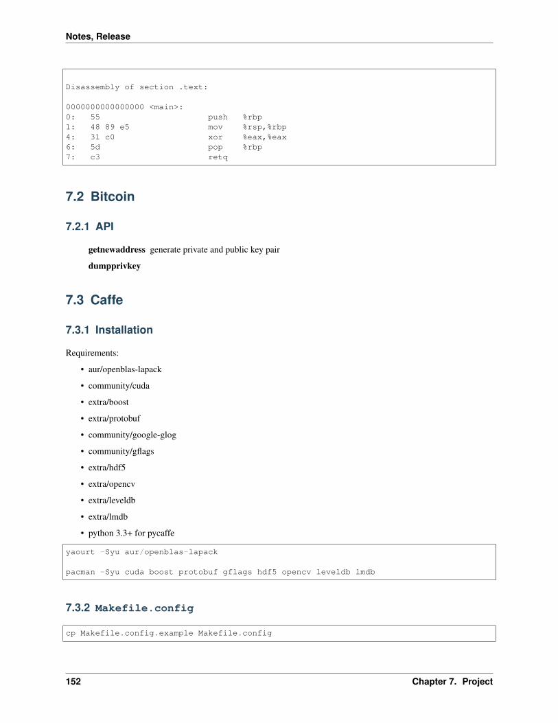
Notes, Release

Disassembly of section .text:

0000000000000000 <main>:0: 55 push %rbp1: 48 89 e5 mov %rsp,%rbp4: 31 c0 xor %eax,%eax6: 5d pop %rbp7: c3 retq

7.2 Bitcoin

7.2.1 API

getnewaddress generate private and public key pair

dumpprivkey

7.3 Caffe

7.3.1 Installation

Requirements:

• aur/openblas-lapack

• community/cuda

• extra/boost

• extra/protobuf

• community/google-glog

• community/gflags

• extra/hdf5

• extra/opencv

• extra/leveldb

• extra/lmdb

• python 3.3+ for pycaffe

yaourt -Syu aur/openblas-lapack

pacman -Syu cuda boost protobuf gflags hdf5 opencv leveldb lmdb

7.3.2 Makefile.config

cp Makefile.config.example Makefile.config

152 Chapter 7. Project

Notes, Release

Patch Makefile.config:

--- Makefile.config.example 2016-03-24 19:34:31.112015456 +0800+++ Makefile.config 2016-03-24 20:40:14.378707671 +0800@@ -5,12 +5,12 @@# USE_CUDNN := 1

# CPU-only switch (uncomment to build without GPU support).-# CPU_ONLY := 1+CPU_ONLY := 1

# uncomment to disable IO dependencies and corresponding data layers-# USE_OPENCV := 0-# USE_LEVELDB := 0-# USE_LMDB := 0+USE_OPENCV := 1+USE_LEVELDB := 1+USE_LMDB := 1

# uncomment to allow MDB_NOLOCK when reading LMDB files (only if necessary)# You should not set this flag if you will be reading LMDBs with any

@@ -25,7 +25,7 @@# CUSTOM_CXX := g++

# CUDA directory contains bin/ and lib/ directories that we need.-CUDA_DIR := /usr/local/cuda+CUDA_DIR := /opt/cuda# On Ubuntu 14.04, if cuda tools are installed via# "sudo apt-get install nvidia-cuda-toolkit" then use this instead:# CUDA_DIR := /usr

@@ -43,7 +43,7 @@# atlas for ATLAS (default)# mkl for MKL# open for OpenBlas

-BLAS := atlas+BLAS := open# Custom (MKL/ATLAS/OpenBLAS) include and lib directories.# Leave commented to accept the defaults for your choice of BLAS# (which should work)!

@@ -61,8 +61,8 @@

# NOTE: this is required only if you will compile the python interface.# We need to be able to find Python.h and numpy/arrayobject.h.

-PYTHON_INCLUDE := /usr/include/python2.7 \- /usr/lib/python2.7/dist-packages/numpy/core/include+# PYTHON_INCLUDE := /usr/include/python2.7 \+# /usr/lib/python2.7/dist-packages/numpy/core/include# Anaconda Python distribution is quite popular. Include path:# Verify anaconda location, sometimes it's in root.# ANACONDA_HOME := $(HOME)/anaconda

@@ -71,9 +71,9 @@# $(ANACONDA_HOME)/lib/python2.7/site-packages/numpy/core/include \

# Uncomment to use Python 3 (default is Python 2)-# PYTHON_LIBRARIES := boost_python3 python3.5m-# PYTHON_INCLUDE := /usr/include/python3.5m \-# /usr/lib/python3.5/dist-packages/numpy/core/include+PYTHON_LIBRARIES := boost_python3 python3.5m+PYTHON_INCLUDE := /usr/include/python3.5m \

7.3. Caffe 153

Notes, Release

+ /usr/lib/python3.5/dist-packages/numpy/core/include

# We need to be able to find libpythonX.X.so or .dylib.PYTHON_LIB := /usr/lib

7.4 Chewing Editor

7.4.1 Installation

My env is Arch Linux.

Requirements

QT = 5

• qt5-tools

• qt5-base

pacman -Ss qt5-base qt5-tools

qt5-tools will provide /usr/lib/qt/bin/lrelease. When building chewing-editor, we will need it.

7.4.2 Issues

#43 - Use system gtest

If gtest do not ship with share library, the default cmake module, FindGTest, will raise error.

ref:

• module FindGTest source

• https://github.com/dmonopoly/gtest-cmake-example

• http://stackoverflow.com/questions/9689183/cmake-googletest

• http://stackoverflow.com/questions/21237341/testing-with-gtest-and-gmock-shared-vs-static-libraries

• http://stackoverflow.com/questions/10765885/how-to-install-your-custom-cmake-find-module

• Ubuntu libgtest-dev package list It’s source only.

7.5 Ethereum

7.5.1 Create Private Network

• Use go-ethereum as client

pkg install net-p2p/go-ethereum

mkdir ~/.ethapc/


https://cmake.org/cmake/help/latest/module/FindGTest.html

https://github.com/Kitware/CMake/blob/master/Modules/FindGTest.cmake

https://github.com/dmonopoly/gtest-cmake-example

http://stackoverflow.com/questions/9689183/cmake-googletest

http://stackoverflow.com/questions/21237341/testing-with-gtest-and-gmock-shared-vs-static-libraries

http://stackoverflow.com/questions/10765885/how-to-install-your-custom-cmake-find-module

http://packages.ubuntu.com/zh-tw/trusty/all/libgtest-dev/filelist

Notes, Release

Create custom genesis block:

cat ~/.ethapc/genesis.json

"alloc" : ,"coinbase" : "0x0000000000000000000000000000000000000000","difficulty" : "0x20000","extraData" : "","gasLimit" : "0x2fefd8","nonce" : "0x0000000000000042","mixhash" : "0x0000000000000000000000000000000000000000000000000000000000000000

→˓","parentHash" : "0x0000000000000000000000000000000000000000000000000000000000000000

→˓","timestamp" : "0x00"

Flags

geth --nodiscover --maxpeers 0 --identity "MyNodeName" --datadir=~/.ethapc --→˓networkid 42

Attach

geth attach ipc:~/.ethapc/geth.ipc

7.6 GnuPG

7.6.1 Cipher

Def An algorithm for performing encryption

Cipher vs Code

Code

• using codebook

• the ciphertext contain all the information of original plaintext

Cipher

• usually depends on a key (or says cryptovariable)

1. https://en.wikipedia.org/wiki/Cipher

7.6.2 Reference

1. https://futureboy.us/pgp.html

2. http://secushare.org/PGP

7.6. GnuPG 155

https://en.wikipedia.org/wiki/Cipher

https://futureboy.us/pgp.html

http://secushare.org/PGP

Notes, Release

7.7 LaTeX

𝐿A𝑇E𝑋

7.7.1 Command

\command[optional param]param

• command starts with \

• whitespace is ignored after commands.

• force whitespace after commands

𝑇E𝑋𝑎𝑛𝑑𝐿A𝑇E𝑋.

7.7.2 Comments

Hello % here is commen, World

e.g.:

𝐻𝑒𝑙𝑙𝑜,𝑊𝑜𝑟𝑙𝑑

7.7.3 File Structure

.tex

\documentclass... % LaTeX2e doc required This\usepackage... % setup

\titletitle\authorIblis Lin

\begindocument

content

\enddocument

• .sty: 𝐿A𝑇E𝑋 package.

7.7.4 Line/page breaking

paragraph a set of words to convey the same, coherent idea. Placing blank line between two paragraph.

line break

• just use \\ or \newline in same paragraph.

• \\*: prohibit page breaking after this new line

• \pagebreak


Notes, Release

7.7.5 Quoting

`` for open'' for close

e.g:

``quoting some text''

7.7.6 Tilde

\~

http://foo/\~bar

7.7.7 Accents

H\^otel, na\"\i ve, \’el\‘eve,\\sm\o rrebr\o d, !‘Se\~norita!,\\Sch\"onbrunner Schlo\ssStra\ss e

7.7.8 TikZ

Preamble:

\usepackagetikz

\begintikzpicture\draw (0, 0) to (2, 2) -- (4, 0) -- cycle;\draw (2, 2) -- (1, 0);

\endtikzpicture

Plot function:

\draw[green, ultra thick, domain=0:0.5] plot (\x, 0.025+\x+\x*\x);

Plot label:

\node [above left] at (1, 1) $x$;

7.8 libuv

Ref: https://nikhilm.github.io/uvbook/index.html

• Async, event-driven style of programming.

• event loop: uv_run()

• I/O blocking : event-loop approach

7.8. libuv 157

https://nikhilm.github.io/uvbook/index.html

Notes, Release

– read, write I/O thread (or thread pool)

– libuv async, non-blocking OS event subsystem:

* Async: X file X

* Non-blocking: X file free to do other task.

7.9 Libvirt

7.9.1 Network

On Arch:

sudo pacman -Syu ebtables dnsmasq firewalldsudo systemctl start firewalldsudo systemctl enable firewalldsudo systemctl restart libvirtd

• Ref: http://demo102.phpcaiji.com/article/bagdcea-libvirt-failed-to-initialize-a-valid-firewall-backend.html

7.10 Make

After FreeBSD 10.0, the implementation of make(1) is bmake(1). pmake(1) is deprecated.

ref: http://www.crufty.net/help/sjg/bmake.html

7.10.1 bmake and gmake compatible Makefile

Quote from stackoverflow:

You could put your GNU-specific stuff in GNUmakefile, your BSD-specific stuff in BSDmakefile,and your common stuff in a file named Makefile.common or similar. Then include Makefile.common at the very beginning of each of the other two. Downside is, now you have 3 makefiles insteadof 2. Upside, you’ll only be editing 1.

bmake

The file BSDmakefile has highest priority.

-[/usr/share/mk]| [Venv(py3)] [-- INSERT --]-[iblis@abeing]% grep BSDmakefile /usr/share/mk/sys.mk.MAKE.MAKEFILE_PREFERENCE= BSDmakefile makefile Makefile

Ref

https://stackoverflow.com/questions/3848656/bsd-make-and-gnu-make-compatible-makefile


http://demo102.phpcaiji.com/article/bagdcea-libvirt-failed-to-initialize-a-valid-firewall-backend.html

http://www.crufty.net/help/sjg/bmake.html

https://stackoverflow.com/questions/3848656/bsd-make-and-gnu-make-compatible-makefile

Notes, Release

7.10.2 bmake Suffix Rules

man make

and search SUFFIXES

.SUFFIXES: .o

.c.o:cc -o $.TARGET -c $.IMPSRC

7.11 MXNet

7.11.1 Compile

Compile on my machine:

mkdir buildcd buildcmake .. -DCUDA_HOST_COMPILER=/opt/cuda/bin/gcc

7.11.2 MXNet.jl

Get network weight

model.arg_params -> DictSymbol => NDArray

Extract data from NDArray

Julia wrapper MXNet NDArray MXNet tensor GPU mx.copy!(Array, NDArray) :

# w is NDArrayarr = zeros(eltype(w), size(w))mx.copy!(arr, w)

or breifly:

# warr = copy(w)

Show net layers:

julia> mx.list_arguments(net)24-element ArraySymbol,1::data:fullyconnected0_weight:fullyconnected0_bias:fullyconnected1_weight:fullyconnected1_bias:fullyconnected2_weight:fullyconnected2_bias:fullyconnected3_weight:fullyconnected3_bias:fullyconnected4_weight:fullyconnected4_bias

7.11. MXNet 159

Notes, Release

:fullyconnected5_weight:fullyconnected5_bias:fullyconnected6_weight:fullyconnected6_bias:fullyconnected7_weight:fullyconnected7_bias:fullyconnected8_weight:fullyconnected8_bias:fullyconnected9_weight:fullyconnected9_bias:fullyconnected10_weight:fullyconnected10_bias:label

7.12 nftable

git clone git://git.netfilter.org/nftables

# load samplenft -f files/nftables/ipv4-filter

7.12.1 Add

nft add rule ip filter input ip saddr '!= 1.2.0.0/16' tcp dport 8545 dropnft list table filter -a

7.12.2 Ref

• https://home.regit.org/netfilter-en/nftables-quick-howto/

7.13 NTP

7.13.1 Arch

Ref: https://wiki.archlinux.org/index.php/Systemd-timesyncd

It’s already included in Systemd:

sudo timedatectl set-ntp truetimedatectl status

That’s all.


https://home.regit.org/netfilter-en/nftables-quick-howto/

https://wiki.archlinux.org/index.php/Systemd-timesyncd

Notes, Release

7.14 OpenCL

7.14.1 Task Parallel

Via Native Kernel, and benifit from some vector types plus SIMT

7.15 pacman

/etc/pacman.conf:

IgnorePkg = linux awesome deluge nvidia nvidia-utils

7.16 sudo

Some distro, like manjaro, override the rule via /etc/sudoers.d/*. So changing the config via visudo maynot work.

7.17 TensorFlow

• General computing platform

Tensor The n-dimension data

Flow The operation

• written in CPP

• offer python interface via SWIG

• GPU support

– Optional

– Linux only

– Cuda Toolkit >= 7.0

7.17.1 Installation

• require gcc

• clone with submodule:

$ git clone --recurse-submodules https://github.com/tensorflow/tensorflow

• build system: Bazel

• build python wheel package:

bazel build -c opt //tensorflow/tools/pip_package:build_pip_package -j 6

• SWIG:

7.14. OpenCL 161

http://bazel.io/

Notes, Release

pacman -S swig

• Pypi:

pip install numpy wheel

Configuring GPU

-[iblis@pandapc Oops]% ./configurePlease specify the location of python. [Default is /home/iblis/venv/py35/bin/python]:Do you wish to build TensorFlow with GPU support? [y/N] yGPU support will be enabled for TensorFlowPlease specify which gcc nvcc should use as the host compiler. [Default is /sbin/→˓gcc]: /usr/bin/gccPlease specify the Cuda SDK version you want to use, e.g. 7.0. [Leave empty to use→˓system default]: 7.5.18Please specify the location where CUDA 7.5.18 toolkit is installed. Refer to README.→˓md for more details. [Default is /usr/local/cuda]: /opt/cudaPlease specify the Cudnn version you want to use. [Leave empty to use system→˓default]: 5.0.4Please specify the location where cuDNN 5.0.4 library is installed. Refer to README.→˓md for more details. [Default is /opt/cuda]:Please specify a list of comma-separated Cuda compute capabilities you want to build→˓with.You can find the compute capability of your device at: https://developer.nvidia.com/→˓cuda-gpus.Please note that each additional compute capability significantly increases your→˓build time and binary size.[Default is: "3.5,5.2"]: 5.0Setting up Cuda includeSetting up Cuda lib64Setting up Cuda binSetting up Cuda nvvmConfiguration finished

Patches

• cc_configure.bzl: For bazel bazel <= 0.2.1

cd tensorflow/tensorflowwget https://github.com/bazelbuild/bazel/blob/master/tools/cpp/cc_configure.→˓bzl

• WORKSPACE

diff --git a/WORKSPACE b/WORKSPACEindex d3e01b7..033685b 100644--- a/WORKSPACE+++ b/WORKSPACE@@ -20,6 +20,9 @@ tf_workspace()load("//tensorflow:tensorflow.bzl", "check_version")check_version("0.1.4")

+# load("//tensorflow:cc_configure.bzl", "cc_configure")


Notes, Release

+# cc_configure()+# TENSORBOARD_BOWER_AUTOGENERATED_BELOW_THIS_LINE_DO_NOT_EDIT

new_git_repository()

• third_party/gpus/crosstool/CROSSTOOL

diff --git a/third_party/gpus/crosstool/CROSSTOOL b/third_party/gpus/crosstool/→˓CROSSTOOLindex a9f26f5..1bc2138 100644--- a/third_party/gpus/crosstool/CROSSTOOL+++ b/third_party/gpus/crosstool/CROSSTOOL@@ -57,6 +105,8 @@ toolchain # used by gcc. That works because bazel currently doesn't track files at# absolute locations and has no remote execution, yet. However, this will need# to be fixed, maybe with auto-detection?+ cxx_builtin_include_directory: "/home/iblis/git/tensorflow/third_party/gpus/cuda/→˓include"+ cxx_builtin_include_directory: "/opt/cuda/include"

7.17.2 2D Conv

input 128x128 rgb 3 channel input tensor 128x128x3

filter 5x5 64 filter -> filter tensor 5x5x64

conv 128x128x3x64 just guessing

7.18 Xorg

7.18.1 Trackball

Get the id:

xinput list

xinput --set-prop 12 "libinput Middle Emulation Enabled" 1

7.19 zsh

7.19.1 Bump Up the File Descriptor Limit

We can set the soft limit up to hard limit.

Check the hard limit:

$ ulimit -Hn4096

Then check the soft limit:

7.18. Xorg 163

Notes, Release

$ ulimit -Sn1024

Bump up it:

$ ulimit -Sn unlimited$ ulimit -Sn4096

7.20 Compiler

7.20.1 Dragon book

Compilers Principles, Techniques and Tools

Introduction

Parts of compiler:

• Front-end

– generate IR (itermediate representation)

–

• Mid-end

• Back-end

–

Generate Object File

prog.c -> pre-proccessing -> prog.s

Quote from clang(1):

Stage Selection Options

-E Run the preprocessor stage.

-fsyntax-only Run the preprocessor, parser and type checking stages.

-S Run the previous stages as well as LLVM generation andoptimization stages and target-specific code generation,producing an assembly file.

-c Run all of the above, plus the assembler, generating a tar-get ”.o” object file.

Structure of Compiler

• token stream

• AST


Notes, Release

• IR: three address code. optimizer IR

• target native code

• symbol table

Phases and Passes

phase compiler

pass phase group compiler read file -> write file

front-end pass

• lexical analysis output token

• syntax analysis or parsing

• semantic analysis type type checking;

type conversion – coercions

• IR code gen:

– syntax tree is a form of IR

– three address code

• symbol table management

optional pass

• optimization

– data-flow optimizations

– instruction level parallelism, e.g. re-order instruction, SIMD

– proccessor level parallelism

– optimization for memory hierarchy

back-end pass

• code gen

Toolchains

parser generator

• PEG.js

• peg

• YACC

• Bison

scanner generator

• lex

• flex

syntax-directed translation engine

7.20. Compiler 165

https://pegjs.org/

https://github.com/pointlander/peg

https://www.gnu.org/software/bison/

https://github.com/westes/flex.git

Notes, Release

code-generator generator

data-flow analysis engine

compiler-contruction toolkits

• RPython

Misc

• compiler-rt platform (e.g. x86 & amd64) object file portability. cross-compiling

• low-level resource allocation C register keyword programmer register register compiler registermanagement policy

lex

definition%%transition ruls%%user defined subroutine

Context Free Grammar

sentence non-terminal

Ambiguous Grammar

Def sentence parse tree

Example operator precedence 1 + 2× 3 parse?

associativity 1 + 2 + 3

Left Recursion

immediate left recursion Eliminating formula: why?

Parsing

LL

LR

Viable Prefix Handle ( Handle)


https://rpython.readthedocs.io/en/latest/

Notes, Release

Semantic Analysis

context-free grammer :

• context-sensitive grammer

• context-free grammer + attribute

2, - SDD: Syntax-Directed Definition

• SDT: Syntax-Directed Translation scheme

7.20. Compiler 167

Notes, Release


Notes, Release

CHAPTER 8

Trading

8.1 TXF

8.1.1 2016-01-27

long-term

170 Chapter 8. Trading

Notes, Release

inter-day

• vol avg(10), attempt to go up, higher va => slowing

• vol avg(10), attempt to down, lower va => non-facilitate? slowing, balancing?

• top @ 7850?

• buttom @ 7600 -> 7640?

short-term

• poc keep moving lower

• early selling tail from 7859 to 7835: 24point

• buying tail quite smaller than selling

• the high/low point support by previous VA

•

– 70

– previous VA: 50 point

•

–

– new seller

8.1. TXF 171

Notes, Release

• 10 am & 12

– seller 7859 -> 7834

– HVA

– slowing

– HVA 2

•

– seller covering

– buyer: 7778 -> 7790: 12 points

30 K

• buyer has logger time-frame

8.2 Market in Profile

8.2.1 Lagger

• non-forced convering, lagger

8.2.2 5/13

• => timeframe

• Peter

– Day TimeFrame (DTF)

– Other TimeFrame (OTF)

Scalper

bid-ask spread

DTF

Day TimeFrame

zero position

Behavior

price /

e.g. DTF buy at 4.99 vol 20 -> 4.98 vol 20 -> 4....

DTF OTF buyer DTF position

Side effect DTF liquidity


Notes, Release

Other TimeFrame

Short-Term Trader

Short-Term

Intermediate-Term Trader

Long-Term Trader

8.2.3 Resting inside a Trend

2016/05

resting bracket

trend

8.2. Market in Profile 173

Notes, Release


CHAPTER 9

Web

9.1 JWT

9.1.1 Resources

• http://www.slideshare.net/stormpath/building-secure-user-interfaces-with-jwts

9.2 Vue

• MVVM pattern

9.2.1 Vue Instance

• data property proxy

• properties created by vue will be prefixed with $. e.g.: vm.$el, vm.$watch

• Instance hook: mounted ... etc.

9.2.2 Slots

Child component:

divh2 I'm the child title

slot| This will only be displayed| if there is no content to be distributed. // fallback content

175

http://www.slideshare.net/stormpath/building-secure-user-interfaces-with-jwts

Notes, Release

Parent::

div h1 I’m the parent title

child-component p This is some original content p This is some more original content

Render:

divh1 I'm the parent title

divh2 I'm the child title

p This is some original contentp This is some more original content

176 Chapter 9. Web

CHAPTER 10

Reading

10.1 Analysis of Financial Time Series

10.1.1 Intro

Assets Returns Scale-free feature. return series price series return definitions.

Simple Gross Return

Single period return.

1 +𝑅𝑡 =𝑃𝑡𝑃𝑡−1

period ,

Multiperiod Simple Return

Hold 𝑘 period. A.k.a compound return.

1 +𝑅𝑡[𝑘] =𝑃𝑡𝑃𝑡−𝑘

=𝑃𝑡𝑃𝑡−1

× 𝑃𝑡−1

𝑃𝑡−2× · · · × 𝑃𝑡−𝑘+1

𝑃𝑡−𝑘

= (1 +𝑅𝑡)(1 +𝑅𝑡−1) . . . (1 +𝑅𝑡−𝑘+1)

=

𝑘−1∏𝑖=0

(1 +𝑅𝑡−𝑖)

Multiperiod single period

Annualized Returns

If we hold 𝑘 years.

𝐴𝑛𝑛𝑢𝑎𝑙𝑖𝑧𝑒𝑑𝑅𝑡[𝑘] = (𝑅𝑡[𝑘])1𝑘 − 1

177

Notes, Release

𝑅𝑡[𝑘] geometric mean, multiperiod period

𝐴𝑛𝑛𝑢𝑎𝑙𝑖𝑧𝑒𝑑𝑅𝑡[𝑘] = exp

[1

𝑘

𝑘−1∑𝑖=0

ln 1 +𝑅𝑡−𝑖

]− 1

Taylor expansion (but why?)

𝐴𝑛𝑛𝑢𝑎𝑙𝑖𝑧𝑒𝑑𝑅𝑡[𝑘] =1

𝑘

𝑘−1∑𝑖=1

𝑅𝑡−𝑗

Countinuous Compounding

• proof

Net value of a asset 𝐴

𝐴 = 𝐶𝑒𝑟𝑚

𝐶 = 𝐴𝑒−𝑟𝑚 (present value)

where 𝑟 is the interest rate per annum, 𝐶 is the initial capital.

present value 5 100 100

Continuously Compounded Return

def natural logarithm of the simple gross return

A.k.a. log return

In one-period:

𝑟𝑡 = ln(1 +𝑅𝑡) = ln𝑃𝑡𝑃𝑡−1

Extend to Multiperiod:

𝑟𝑡[𝑘] = ln(1 +𝑅𝑡[𝑘])

= ln

[𝑘−1∏𝑖=0

(1 +𝑅𝑡−𝑖)

]

=

𝑘−1∑𝑖=0

ln(1 +𝑅𝑡−𝑖)

=

𝑘−1∑𝑖=0

𝑟𝑡−𝑖

multiperiod one-period sum

Portfolio Return

simple portfolio return simple return weighting

continuously compounded protfolio return 𝑟𝑝,𝑡 ≈∑𝑤𝑖𝑟𝑖𝑡, assumption: “simple returns Rit are all small

in magnitude” (?)

Excess Return

risk free asset return

long asset + short risk free asset total return

178 Chapter 10. Reading

http://www-stat.wharton.upenn.edu/~waterman/Teaching/IntroMath99/Class04/Notes/node13.htm

CHAPTER 11

Misc

11.1 Fonts

11.1.1 Installation

1. Copy to ~/.local/share/fonts (~/.fonts is deprecated)

2. fc-cache -fv

11.1.2 CNS11643

http://data.gov.tw/node/5961

• License: http://data.gov.tw/license

179

http://data.gov.tw/node/5961

http://data.gov.tw/license

Notes, Release

180 Chapter 11. Misc

CHAPTER 12

Indices and tables

• genindex

• search

181

Notes - media.readthedocs.org · Iblis Lin Nov 21, 2017. Contents 1 Algorithm 3 2 Database 75 3...

Documents

Transcript of Notes - media.readthedocs.org · Iblis Lin Nov 21, 2017. Contents 1 Algorithm 3 2 Database 75 3...