Notes for Math 471 { Real Analysis Measure and...

$: Notes for Math 471 { Real Analysis Measure and …web.math.rochester.edu/people/grads/clungstr/real_analysis/Notes.pdfNotes for Math 471 { Real Analysis Measure and Integral by Wheeden$
Notes forMath 471 – Real Analysis

Measure and Integral by Wheeden and Zygmund

Clayton J. Lungstrum

December 8, 2012

HW: Chapter 1: pp. 13-14, #16,17 Chapter 2: p. 31, #1,5,6

1 The Riemann Integral

We begin with a sample of things we hope to see later in the course.

Definition 1.1. A function f is said to vanish at infinity if for all ε > 0 there is a compactset K ⊆ X such that x ∈ KC implies |f(x)| < ε.

Theorem (Riesz). Let X be a locally compact, regular topological space. Let C0(X) bethe space of continuous functions which vanish at infinity. Then the space of bounded linearfunctionals on C0(X) can be identified with the space of Borel measures on X.

Remark 1.1. C0(X)∗ is the dual space of C0(X, i.e., the set{L : C0 → C : |L(f)| ≤ C · sup

x∈X|f(x)| for some C ∈ R

}.

This means, L ∈ C0(X)∗ implies there exists a unique Borel measure µ on X such thatL(f) =

∫Xf(x)dµ(x).

Example 1.1. Fix x0 ∈ X, and consider

Lx0(f) = f(x0), Lx0 ∈ C0(X)∗ =

∫X

f(x)dµx0(x)

where µx0 is the Dirac delta measure.

We’ll begin by covering concrete measure theory; that is, Lebesgue measure on Rn, n ≥ 1.Lebesgue measure of the measure sets E ⊆ Rn is similar to defining the volume of sets. Alongthe way we’ll need to define measurable functions f : Rn → R, as well as integration overmeasurable functions. After defining these, we’ll discuss various properties of the integral,such as changing the order of integration (Fubini’s Theorem) and interchanging limits andintegrals (Lebesgue Dominated Convergence Theorem).

Finally, let us now begin by recalling Riemann integration on R.

Definition 1.2. A partition Γ of an interval [a, b] is a finite set of points {a = x0 < x1 <· · · < xN = b}.Definition 1.3. The norm (or mesh size) is |Γ| = max1≤j≤N |xj − xj−1|.Definition 1.4. The Riemann sum is defined by

SΓ =N∑j=1

f(ξj)(xj − xj−1),

where the ξj’s are sample points chosen from the interval [xj−1, xj]. We will say that f isRiemann integrable if lim|Γ|→0 SΓ exists. That is, if there exists an A ∈ R such that for everyε > 0 there exists a δ > 0 such that |Γ| < δ implies |SΓ − A| < ε. Denote A by

(R)

∫ b

a

f(x)dx.

1

Theorem 1.1. If f is continuous on [a, b], then f is Riemann integrable.

Example 1.2. An example that requires something more than simply discontinuous is theDirichlet function, i.e.,

f(x) =

{1 : x ∈ Q0 : x ∈ R \Q

.

This function is not integrable on any non-degenerate interval.

2 Functions of Bounded Variation

Definition 2.1. Let f : [a, b] → R and Γ be a partition of [a, b]. Define the variation off relative to Γ to be

SΓ(f ; [a, b]) =N∑j=1

|f(xj)− f(xj−1)|.

Define the total variation of f on [a, b] to be

V (f ; [a, b]) = V (f) = supΓSΓ(f ; [a, b]).

Definition 2.2. We say that f is of bounded variation if V (f) <∞ and f is of unboundedvariation if V (f) =∞.

Example 2.1. If f is monotonic on [a, b], then V (f) = |f(b)− f(a)|, depending on whetheror not it is increasing or decreasing.

Definition 2.3. A function f defined on [a, b] is said to satisfy a Lipschitz condition on[a, b], or to be a Lipschitz function on [a, b], if there is a constant C such that

|f(x)− f(y)| ≤ C|x− y| for all x, y ∈ [a, b].

Example 2.2. If f ∈ C1[a, b], then

|f(x)− f(y)| =∣∣∣∣∫ x

y

f ′(s)ds

∣∣∣∣≤∫ x

y

|f ′(s)| ds

≤M(x− y)

where |f ′(x)| ≤M for all x ∈ [a, b] which exists since it is the continuous image of a compactset. Thus all continuously differentiable functions are Lipschitz functions.

Proposition 2.1. Let f satisfy a Lipschitz condition. Then f is of bounded variation.

2

Proof.

SΓ =N∑j=1

|f(xj)− f(xj−1|

≤N∑j=1

C|xj − xj−1|

= C(b− a) <∞.

Thus, we have that V (f) ≤ C(b− a).Q.E.D.

Note 2.1. We will denote the vector space of all functions of bounded variation on [a, b] byBV [a, b].

At this point, it may be useful to note that C1[a, b] ⊆ Lip[a, b] ⊆ BV [a, b].

Note 2.2. BV [a, b] is a normed linear vector space with ‖f‖ = V (f).

Theorem 2.1.

(i) If [a′, b′] ⊆ [a, b], then V (f ; [a′, b′]) ≤ V (f ; [a, b]).

(ii) If a < c < b, then V (f ; [a, b]) <∞ implies V (f ; [a, b]) = V (f ; [a, c]) + V (f ; [c, b]).

Proof. For a proof, refer to the text.Q.E.D.

Now we will introduce the concepts of positive and negative variation, which, as theirname implies, measures how much upward variation the function has (positive) and howmuch downward variation the function has (negative).

Definition 2.4. For x ∈ R, define the following:

x+ =

{x : x > 0

0 : x ≤ 0and x− =

{0 : x > 0

x : x ≤ 0

Note 2.3. It will be useful to note that |x| = x+ + x−, x = x+ − x−, x+ = 12

(x+ |x|

), and

x− = 12

(|x| − x

).

Define

PΓ(f) =n∑j=1

[f(xj)− f(xj−1)

]+

NΓ(f) =n∑j=1

[f(xj)− f(xj−1)

]−

to be the positive and negative variation with respect to the partition Γ.

3

Note 2.4. PΓ(f)−NΓ(f) =∑n

j=1 f(xj)− f(xj−1) = f(b)− f(a)

Definition 2.5. The positive and negative variations of f on [a, b] are

P = P (f) = supΓPΓ(f) and N = N(f) = sup

ΓNΓ(f)

Theorem 2.2. If f is a bounded function on [a, b], then if any one of P , N , or V is finite,then the other two are finite as well, and

P +N = V ; P −N = f(b)− f(a).

Proof. Confer the text.Q.E.D.

Corollary 2.1 (Jordan’s Theorem). A function f is of bounded variation if and only iff = f1 − f2 are bounded, increasing functions. Equivalently, f = f1 + f2, where f1 is abounded, increasing function and f2 is a bounded, decreasing function.

Proof. Suppose f = f1 − f2, then since f1, f2 ∈ BV [a, b] and BV is a linear space, f1 − f2 ∈BV [a, b].

Conversely, refer to the text.Q.E.D.

Definition 2.6. We say f has a discontinuity of the first kind at a if f(a+) =limx→a+ f(x) and f(a−) = limx→a− f(x) both exist. If f(a+) = f(a−), we can redefine f ata to be this common value and say f has a removable discontinuity at a. If f(a+) 6= f(a−),then f has a jump discontinuity at a.

Note that if f is monotonic and bounded, then any discontinuities are of the first kindsince f(a+) and f(a−) exist by basic real analysis.

Theorem 2.3. A function f ∈ BV [α, β] implies f only has discontinuities of the first kindand there are at most countably many.

Proof. If f ∈ BV [α, β], write f = f1 − f2 with f1 and f2 increasing. It suffices to provethe theorem for each of f1 and f2 separately, so let us treat f1, replacing it by f2 for thesecond part. We know that f1 only has discontinuities of the first kind, and it is sufficient toassume only jump discontinuities occur since removable discontinuities only occur at pointsfor which the function is not defined, hence they’re not “really” discontinuities. Let

D1 = {a ∈ [α, β] : f1 has a discontinuity at a}

=∞⋃k=1

{a ∈ [α, β] : f1(a+)− f1(a−) >1

k}.

Since f1 is bounded, the cardinality of D1 is at most countable.Following the same process for f2, we have the same conclusion, and the countable union

of countable sets is countable, thus the set of discontinuities are at most countable.Q.E.D.

4

Theorem 2.4. If f ∈ C[a, b], then V (f) = lim|Γ|→0 SΓ(f); i.e., for every ε > 0 there existsa δ > 0 such that |Γ| < δ implies SΓ > V (f)− ε.

Proof. Refer to the text for the proof.Q.E.D.

Theorem 2.5. If f ∈ C1[a, b], then

V (f) = (R)

∫ b

a

|f ′(x)|dx

N(f) = (R)

∫ b

a

(f−(x))−dx

P (f) = (R)

∫ b

a

(f+(x))+dx

Proof. Since f ∈ C1[a, b], we can apply the Mean Value Theorem to each of the subintervalsdetermined by the partition, thus we have for some points ξj,

f(xj)− f(xj−1) = f ′(ξj)(xj − xj−1).

This implies

SΓ(f) =n∑j=1

|f ′(x)|(xj − xj−1)

which is the Riemann sum on [a, b]. Since |f ′| ∈ C[a, b], the theory of Riemann integrationimplies

lim|Γ|→0

SΓ(f) = (R)

∫ b

a

|f ′(x)|dx,

and thus lim|Γ|→0 = V (f).Q.E.D.

Note 2.5. We have the following:

(i) P +N = V

(ii) P −N = f(b)− f(a)

(iii)

P =1

2

[V + f(b)− f(a)

]=

1

2

[ ∫ b

a

|f ′(x)|dx =

∫ b

a

f ′(x)dx

]=

∫ b

a

1

2

[|f ′(x)|+ f(x)

]dx

=

∫ b

a

(f ′(x))+dx

5

Now let us turn our attention to rectifiable curves. We’ll consider these curves in theplane, R2 for simplicity, though for Rn the process is almost the same. A curve has aparametric representation as follows:

C =

{φ(t) : a ≤ t ≤ b

ψ(t) : a ≤ t ≤ b.

Definition 2.7. The graph or image of C is {(φ(t), ψ(t)) : a ≤ t ≤ b} ⊆ R2.

For these curves, we’ll consider polygonal approximations and measure the length of theseapproximations. To that end, let Γ = {a = t0 < t1 < · · · < tn = b} be a partition of [a, b].Let Pj = (φ(tj), ψ(tj)) and approximate C by the union of the line segments Pj−1Pj. Observethat these are polygonal, i.e., piecewise linear, approximations to C.Definition 2.8. Define the geometric length of CΓ to be

`(Γ) =n∑j=1

∣∣Pj−1Pj∣∣

=n∑j=1

[(φ(tj)− φ(tj−1))2 + (ψ(tj)− ψ(tj−1))2]1/2 .

Definition 2.9.

(i) L=L(C)=supΓ `(Γ), 0 ≤ L ≤ ∞;

(ii) C is rectifiable if L <∞.

Note 2.6. Rectifiability is a property of the parametric curve, not its graph.

Example 2.3. Let φ /∈ BV [−1, 1], but −1 ≤ φ(t) ≤ 1 for all t ∈ [−1, 1]. Then C ={(φ(t), ψ(t)) : −1 ≤ t ≤ 1} is not rectifiable even though it is contained in a line segment.For a proof of this, see the following theorem.

Theorem 2.6. A parametric curve C, given by functions φ(t) and ψ(t) on [a, b] is rectifiableif and only if both φ(t) and ψ(t) are of bounded variation. In that case,

max{V (φ), V (ψ)} ≤ L ≤ V (φ) + V (ψ).

HW: Due Thursday, 09/13/2012, Chapter 2 pp. 31–32, #9, 11, 13, 18

Now we shall present our final remarks on functions of bounded variation. First, we’lldiscuss extensions of functions of bounded variation to the complex number system, andwe’ll conclude with the notion of bounded variation on intervals other than closed intervals.

Let f : [a, b]→ C be a complex-valued function, and define SΓ(f) by

SΓ(f) =n∑i=1

∣∣f(xi)− f(xi−1)∣∣

and V (f) by taking the supremum over all partitions of SΓ(f). Since z = x + ıy andmax{|x|, |y|} ≤ |z| ≤ |x| + |y|, we have f ∈ BV [a, b] if and only if Re(f) and Im(f) are ofbounded variation.

6

Definition 2.10. We’ll define f ∈ BV (a, b) if and only if for all a < a′ < b′ < b, f ∈BV [a′, b′] and supa<a′<b′<b V (f ; [a′, b′]) <∞. Similarly, f ∈ BV (R if and only if f ∈ BV [a, b]for −∞ < a < b <∞ and sup−∞<a<b<∞ V (f ; [a, b]) <∞.

3 The Riemann-Stieltjes Integral

If we recall Riemann integration, we would have integrals like the following:∫ bafdx. The

Riemann-Stieltjes integral replaces the x in dx with a more general φ(x). We’ll start with apartition Γ of [a, b] and sample points within the subintervals of the partition, and we willdefine the Riemann-Stieltjes integral in a similar fashion as the standard Riemann integral.More formally, we write for the Riemann-Stieltjes sum with respect to φ as:

RΓ =n∑i=1

f(ξi)[φ(xi)− φ(xi−1)].

Notice this becomes the standard Riemann sum if φ(x) = x.

Definition 3.1. If lim|Γ|→0RΓ = I exists, i.e., for all ε > 0 there exists a δ > 0 such that|Γ| < δ implies |RΓ − I| < ε, then we say that the Riemann-Stieltjes integral of f withrespect to φ exists, written as ∫ b

a

f(x)dφ(x) =

∫ b

a

fdφ,

and we say that f is Riemann-Stieltjes integrable with respect to φ.

Note 3.1.

(i) An equivalent condition is the following: for all ε > 0, there exists a δ > 0 such that|Γ|, |Γ′| < δ implies |RΓ −RΓ′| < ε.

(ii) For φ(x) = x, the notion of Riemann-Stieltjes integrability agrees with Riemann inte-

grability and the value of∫ bafdφ is the same.

(iii) If f ∈ C[a, b] and φ ∈ C1[a, b], then∫ bafdφ =

∫ bafφ′dx.

Proof. Any RΓ =∑n

i=1 f(xi)[φ(xi)− φ(xi−1)], each φ(xi)− φ(xi−1) = φ′(ξi)(xi − xi−1)by the Mean Value Theorem, thus

RΓ =n∑i=1

f(xi)φ′(ξi)(xi − xi−1)

=n∑i=1

(f · φ′)(ξi)(xi − xi−1) +n∑i=1

(f(xi)− f(ξi))φ′(ξi)(xi − xi−1)

It suffices to show the last term tends to zero as the norm of the partition tends tozero. However, because f is continuous on a compact set, we have that it is uniformly

7

continuous, and similarly, since φ′ is continuous on a compact set, its image is boundedby a positive integer, say M . Hence, let δ > 0 such that |f(x) − f(y)| < ε

M(b−a)if

|x− y| < δ. Thus, we have:

n∑i=1

(f(xi)− f(ξi))φ′(ξi)(xi − xi−1) <

ε

M(b− a)

n∑i=1

|φ′(ξi)|(xi − xi−1)

≤ ε

(b− a)

n∑i=1

(xi − xi−1)

≤ ε.

Thus, the right-hand term is ‘small’ for sufficiently large values of n, thus the desiredresult follows.

Q.E.D.

(iv) Suppose φ is a step function, i.e., it is piecewise constant. An equivalent expression isto say there exists a partition A = {a = α0 < α1 < · · · < αn = b} with φ constanton the open intervals (αi−1, αi). Let di = φ(α+

i ) − φ(α−i−1), 1 ≤ i ≤ n − 1, withd0 = φ(a+)− φ(a) and dn = φ(b)− φ(b−). Our claim is:∫ b

a

fdφ =n∑i=0

f(αi)di

as long as C ∈ [a, b].

Theorem 3.1. A necessary condition for∫ bafdφ to exist is for f and φ to have no common

point of discontinuity.

Proof. Refer to the text.Q.E.D.

Theorem 3.2 (Linearity Properties).

(i)∫ bac1f1 + c2f2dφ = c1

∫ baf1dφ + c2

∫ baf2dφ if the two integrals on the right-hand side

exist.

(ii)∫ bafd(c1φ1 + c2φ2) = c1

∫ bafdφ1 + c2

∫ bafdφ2 if the two integrals on the right-hand side

exist.

Thus we can say the map (f, φ) →∫ bafdφ is bilinear; i.e., it is linear in each of the two

components separately.

Note 3.2. This is defined on some linear space containing C[a, b]× C1[a, b].

Theorem 3.3 (Additivity on Intervals).∫ bafdφ =

∫ cafdφ+

∫ bcfdφ for all a < c < b, if the

integral on the left-hand side exists.

Note 3.3. The converse of the preceding theorem fails ! See the book for further details.

8

Theorem 3.4 (Integration by Parts). If f and φ are bounded on [a, b], then if∫ bafdφ exists,

so does∫ baφdf and

∫ bafdφ = f(b)φ(b)− f(a)φ(a)−

∫ baφdf .

Proof. A typical Riemann-Stieltjes sum of∫ bafdφ is

RΓ =n∑i=1

f(ξi)[φ(xi)− φ(xi−1)]

=n∑i=1

f(ξi)φ(xi)−n∑i=1

f(ξi)φ(xi−1)

=n∑i=1

f(ξi)φ(xi)−n−1∑i=0

f(ξi+1)φ(xi)

= −n−1∑i=1

φ(xi)[f(ξi+1)− f(ξi)] + f(ξn)φ(b)− f(ξ1)]φ(a).

Now add and subtract the term φ(a)[f(ξi)−f(a)]+φ(b)[f(b)−f(ξn)], then do some algebra,and we get

RΓ = f(b)φ(b)− f(a)φ(a)− TΓ

where

TΓ =n−1∑i=1

[φ(xi)[f(ξi+1)− f(ξi)]

]+ φ(a)[f(ξ1)− f(a)] + φ(b)[f(b)− f(ξn)].

This is a Riemann-Stieltjes sum of φ with respect to f with partition Γ′ = {a = ξ0 ≤ ξ1 ≤· · · ≤ ξn ≤ ξn+1 = b} with sample points Γ. Note that |Γ′| → 0 as |Γ| → 0, thus lim|Γ|→0RΓ

exists implies lim|Γ′|→0 TΓ exists.Q.E.D.

Now assume that φ is increasing and bounded so that φ(xi) − φ(xi−1) ≥ 0 for all i andall partitions and assume that f is continuous so that

mi = infx∈[xi−1,xi]

f(x) and Mi = supx∈[xi−1,xi]

f(x)

exist. Then, for any sample points {ξi}, we have

n∑i=1

mi(φ(xi)− φ(xi−1)) = LΓ ≤ RΓ ≤ UΓ =n∑i=1

Mi(φ(xi)− φ(xi−1)).

Recall the definition of refinement, i.e., Γ′ is a refinement of Γ if Γ ⊆ Γ′. If Γ,Γ′ are any twopartitions, then Γ′′ = Γ ∪ Γ′ is a common refinement with |Γ′′| ≤ min{|Γ|, |Γ′|}.

Lemma 3.1.

(i) If Γ ⊆ Γ′, then LΓ ≤ LΓ′ and UΓ′ ≤ UΓ.

9

(ii) If Γ, Γ′ are any two partitions, LΓ ≤ UΓ′.


Theorem 3.5. If f ∈ C[a, b], φ ∈ BV [a, b], then∫ bafdφ exists and∣∣∣∣∫ b

a

fdφ

∣∣∣∣ ≤∣∣∣∣∣ supx∈[a,b]

f(x)

∣∣∣∣∣ · V (φ; [a, b]).

4 Lebesgue Measure on Rn

Definition 4.1. An n-dimensional interval is I ⊆ Rn where I =∏n

j=1[aj, bj]. Thevolume of I is v(I) =

∏nj=1(bj − aj).

Definition 4.2. A cover of a set E ⊆ Rn is a countable collection S = {Si}∞i=1 of sets withE ⊆

⋃∞i=1 Si.

We are interested in covers which consist of intervals, S = {Ik}∞i=1. Define

σ(I) =∞∑k=1

v(Ik).

Definition 4.3. For E ⊆ Rn, the Lebesgue outer measure of E, denoted |E|e, is

|E|e = inf{σ(S) : all countable covers of E by rectangles}.

We say that E is a set of Lebesgue measure zero if |E|e=0. More formally, for everyε > 0, there exists a cover S = {Ik}∞k=1, E ⊆

⋃∞k=1 Ik, and

∑∞k=1 v(Ik) < ε. E is considered

a null set since it has measure zero.

Theorem 4.1. If E = I is an interval, then |I|e = v(I).

Proof. Note S = {I} is a cover of I, thus |I|e ≤ σ(S) = v(I). For the reverse inequality, weremark that if I is an n-dimensional interval and 0 < r <∞, let rI denote the interval withthe same center as I and side lengths equal to r times the corresponding side length. Thenv(rI) = rnv(I). Now, suppose S = {Ik}∞k=1 is a cover of I. Let ε > 0 and I∗k = (1+ε)Ik so thatv(I∗k) = (1 + ε)nv(Ik). Now we have I ⊆

⋃∞k=1 Ik ⊆

⋃∞k=1 I

∗k . Note also that I ⊆

⋃∞k=1(I∗k)◦,

which implies {(I∗k)◦}∞k=1 is an open cover of a compact set. By the Heine-Borel theorem,there exists a finite subcover. Relabeling if necessary, we can assume I ⊆

⋃Nk=1(I∗k)◦, thus

v(I) ≤N∑k=1

v(I∗k)

= (1 + ε)nN∑k=1

v(Ik)

≤ (1 + ε)nσ(S).

Since this holds for every ε > 0, we have v(I) ≤ σ(S) for every cover S of I. Taking theinfimum, we get v(I) ≤ |(|eE), and hence, v(I) = |E|e.

Q.E.D.

10

Theorem 4.2 (Monotonicity). If E1 ⊆ E2, then |E1|e ≤ |E2|e.

Proof. Let Sj be the family of all covers Sj b intervals of Ej. It’s clear that any cover of E2

is also a cover of E1, thus S1 ⊆ S2 and |E1|e = infS∈S1 σ(S) ≤ infS∈S2 σ(S) = |E2|e.Q.E.D.

Theorem 4.3. If E =⋃∞k=1 Ek, then |E|e ≤

∑∞k=1 |Ek|e.


Example 4.1. A singleton {x0} ⊆ Rn can be covered by

n∏j=1

[πj(x0)− ε

2, πj(x0) +

ε

2] = Iε.

Then σ(S) = v(Iε) = εn, which converges to 0 as ε tends to 0. That is,

0 ≤ |E|e ≤ infε>0

εn = 0,

hence |E|e=0.

Corollary 4.1. If E ⊆ Rn is countable, then |E|e = 0. Note that even though Qn is densein Rn, it is countable and therefore has measure zero.

Example 4.2. Let P ⊆ Rn be an affine k-plane, 1 ≤ k ≤ n − 1, i.e., P = Π + a for somea ∈ Rn and some k-dimensional linear subspace Π ( Rn.

Claim 4.1. |P |e=0, for a k = n− 1-dimensional hyperplane.

Proof. By remarks below, we can assume P = {x ∈ Rn : xn = 0}. Write P =⋃∞k=1 Pk,

where Pk = {x ∈ Rn : xn = 0, |xj| ≤ k, 1 ≤ j ≤ n−1}. This implies that |P |e ≤∑∞

k=1 |Pk|e.

Claim 4.2. For all k ∈ N, |Pk|e = 0.

Proof. For all ε > 0, consider

Iε =

(n−1∏j=1

[−k, k]

)× [−ε, ε].

Now,v(Iε) = (2k)n−1 · (2ε) = (2nkn−1)ε

which approaches zero as ε approaches zero. Hence, |Pk|e=0, as desired.Q.E.D.

Returning to the claim above, we now have |P |e ≤∑∞

k=1 |Pk|e = 0, thus, |P |e = 0.Q.E.D.

For the remarks cited above, we mean specifically the symmetries of |·|e, i.e.,

11

(1) Translation Invariance; that is, for any a ∈ Rn, E + a = {x + a : x ∈ E} and|E + a|e = |E|e.

(2) Rotation Invariance (defined below)

Definition 4.4. The rotation group in Rn is O(n) = {R ∈ Mn×n(R) : RTR = In = RRT}.If E ⊆ Rn, R ∈ O(n), then R(E) = {Rx : x ∈ E}.

Proposition 4.1. |R(E)|e = |E|e, for all E ⊆ Rn, R ∈ O(n).

(3) Scaling or homogeneity

Definition 4.5. Let r ∈ (0,∞), E ⊆ Rn. Then rE = {rx : x ∈ E}. [Note that this conflictswith the earlier rI.] For every interval I, we have v(rI) = rnv(I).

Proposition 4.2. |rE|e = rn|E|e for 0 < r <∞.

Theorem 4.4. If E ⊆ Rn and ε > 0, then there exists an open set G ⊆ Rn with E ⊆ G,|G|e ≤ |E|e + ε.

Proof. Let ε > 0. There exists a cover S = {Ik}∞k=1 with∑∞

k=1 v(Ik) ≤ |E|e + ε2. Let I∗k be

an open interval containing Ik and with v(I∗k) ≤ v(Ik) + ε2k+1 . Let G =

⋃∞k=1 I

∗k (which is

open), then E ⊆⋃∞k=1 Ik ⊆ G. We have

|G|e =

∣∣∣∣∣∞⋃k=1

I∗k

∣∣∣∣∣≤

∞∑k=1

|I∗k |e

≤∞∑k=1

v(Ik) +ε

2k+1

≤ |E|e +ε

2+ε

2= |E|e + ε

Q.E.D.

Theorem 4.5. If E ⊆ Rn, there exists a Gδ-set with E ⊆ H and |E|e = |H|e.

HW: pp.47–48, #2, 3, 9, 10, 13

Definition 4.6. For all E ⊆ Rn, let S = {Ik}∞k=1 be a cover with each Ik a closed interval.Define σ(S) =

∑∞k=1 v(Ik), and then 0 ≤ σ(S) ≤ ∞. Then the Lebesgue outer measure

of E is|E|e = inf{σ(S) : S is a cover of E.

12

Now we will restrict our attention to M ⊆ 2Rn , the measurable sets as a subset of thepower set of Rn.

Definition 4.7. E ⊆ Rn is (Lebesgue) measurable if for every ε > 0, there exists anopen set G ⊆ Rn such that E ⊆ G and |G− E|e < ε.

Note 4.1. If we write G = E ∪ (G− E), by subadditivity, this implies

|E|e ≤ |E|e + |G− E|e.

Thus, the previous material does not imply the definition of Lebesgue measurability.

We would like to point out that M ( 2Rn ; in particular, there exist nonmeasurablesubsets.

Note 4.2. We would like to list some properties of measurable sets.

(i) |∅|e = 0

(ii) Any open set G is measurable

(iii) Any E such that |E|e = 0 is measurable.

Let us prove the last statement:

Proof. Given ε > 0, there exists a cover S = {Ik}∞k=1 of E such that∑∞

k=1 <ε2. Similar

to before, we can dilate each Ik by r = 21n and call the result I∗k . Then v(I∗k) = 2v(Ik),

and hence E ⊆ (I∗k)◦, which is open. Let G =⋃

(I∗k)◦. Clearly G − E ⊆ G, hence, bysubadditivity we have

|GE|e ≤ |G|e=∣∣∣⋃(I∗k)◦

∣∣∣e

≤∞∑k=1

v(I∗k)◦

< ε.

Therefore, we have satisfied the definition of Lebesgue measurable.Q.E.D.

If E ∈M, we refer to |E|e as just the measure of E. Thus, |E|e = 0 implies |E| = 0.

Corollary 4.2. Any subset of any affine k-plane is measurable and of measure zero.

Theorem 4.6. If {Ek}∞k=1 is a countable collection of measurable sets, then⋃∞k=1Ek ∈ M

and ∣∣∣∣∣∞⋃k=1

Ek

∣∣∣∣∣ ≤∞∑k=1

|Ek|.

13

Proof. By subadditivity, it suffices to show⋃∞k=1Ek ∈ M. To that end, let ε > 0. For each

k, there exists an open set Gk that contains Ek such that |Gk − Ek| < ε2k

. Let G =⋃Gk,

thus G is open,⋃Ek ⊆ G, and∣∣∣G−⋃Ek

∣∣∣ =∣∣∣⋃Gk −

⋃Ek

∣∣∣≤∣∣∣⋃(Gk − Ek)

∣∣∣≤

∞∑k=1

ε

2k

= ε.

Thus, we have that⋃Ek is measurable.

Q.E.D.

Corollary 4.3. Any closed interval is measurable and v(I) = |I|.

Proof. We know I = I◦ ∪ ∂I, I◦ ∈ M, and |∂I|e = 0, thus |∂I| = 0, i.e., ∂I ∈ M and, bythe preceding theorem, I ∈M. Then,

v(I) ≤ |I◦| ≤ |I| ≤ |I◦|+ |∂I| = |I◦| = v(I).

Q.E.D.

Lemma 4.1. If E1, E2 ⊆ Rn and

d(E1, E2) = infx∈E1, y∈E2

|x− y| > 0,

then |E1 ∪ E2|e = |E1|e + |E2|e.

Theorem 4.7. If F ⊆ Rn is closed, then F ∈M.


Theorem 4.8. E ∈M if and only if EC ∈M, where EC = Rn − E.

Proof. If E ∈M, then for every k ∈ N, there exists an open set Gk with E ⊆ Gk, |Gk−E| <1k. We have GC

k ⊆ EC , and GCk is closed, thus is measurable by the previous theorem.

Thus, H =⋃GCk is a countable union of measurable sets, hence is measurable. Therefore,

EC = H ∪ (EC −H), and EC −H ⊆ EC ∩Gk = Gk−E. Thus,∣∣EC −H

∣∣e≤ |Gk − E|e <

1k

which implies∣∣EC −H

∣∣e

= 0, thus EC −H is measurable. Now, EC = H ∪EC −H ∈M.Q.E.D.

Theorem 4.9. If {Ek}∞k=1 are measurable, then E =⋂∞k=1Ek is measurable, and if E1, E2 ∈

M, then E1 − E2 ∈M.

14

Proof. Since E1 − E2 = E1 ∩ EC2 , it suffices to show the first part of the theorem. But, by

the inversion of DeMorgan’s Law, we have

E =∞⋂k=1

Ek =

(∞⋃k=1

ECk

)C

.

Thus, by previous theorems, we have that E ∈M.Q.E.D.

Now let us discuss some abstract topics to make them more accessible later on in thecourse. If X is any set, denote the power set of X by 2X .

Definition 4.8. Σ ∈ 2X is a σ-algebra if it is closed under complements and countableintersections.

Remark 4.1. It is easy to show that for any σ-algebra, ∅, X ∈ Σ. Just take E ∈ Σ, thenE ∩ EC = ∅ ∈ Σ, and the complement of ∅ is the whole space X.

It’s clear that 2X is a σ-algebra since it consists of all subsets of X. We can summarizewhat we’ve done with the measurable sets in the following theorem.

Theorem 4.10. M is a σ-algebra.

Proposition 4.3. Let X be a set and let F be a set of σ-algebras on X. Then F is closedunder intersections.

Proof. Let {Σ}i∈I be a family of σ-algebras and let Σ =⋂i∈I Σi. If E ∈ Σ, then E ∈ Σi

for all i ∈ I, and since each Σi is a σ-algebra, EC is in each Σi, thus EC ∈ Σ. A similarargument holds for the intersection of any countable collection of sets in Σ.

Q.E.D.

If S ⊆ 2X is an arbitrary collection of sets, then let

FS ={

Σ ⊆ 2X : Σ is a σ-algebra and S ⊆ Σ}.

Observe that FS 6= ∅ since 2X is a σ-algebra. Then

Σ =⋂{

Σ : Σ ∈ FS}

is the smallest σ-algebra generated by S.

Example 4.3. Let X = Rn, S be the collection of all open subsets of Rn. S is clearly nota σ-algebra, but, by the process above, S generates a σ-algebra. This is known as the Borelσ-algebra on Rn and is denoted by B, in honor of Emile Borel.

SinceM contains all of the open sets and is a σ-algebra, and B is the smallest σ-algebracontaining the open sets, we have B ⊆M. It can be shown B ⊆M.

Example 4.4. M ⊆ 2Rn , the measurable subsets of Rn. Note that τ (M, where τ is thetopology on Rn.

Let (X, τ) be any topological space. Taking S = τ , the minimal σ-algebra containing τis denoted B, the Borel σ-algebra on X.

Theorem 4.11. On Rn, B (M.

15

4.0.1 Two Important Properties of M

Recall E ⊆ Rn is measurable if and only if for every ε > 0, there exists an open set G suchthat E ⊆ G and |G− E|e < ε.

Lemma 4.2. E is measurable if and only if for every ε > 0, there exists a closed set F ⊆ Esuch that |E − F |e < ε.

Proof. We know E is measurable if and only if EC is measurable, which is measurable if andonly if for every ε > 0 there exists an open set G such that EC ⊆ G and

∣∣G− EC∣∣e< ε.

Thus, writing this as

G− EC = G ∩ (EC)C = G ∩ E = E ∩ (GC)C = E −GC .

Now we have∣∣G− EC

∣∣e< ε if and only if

∣∣E −GC∣∣e< ε. Hence, just take F = GC .

Q.E.D.

Recall the property outer measure subadditivity, and if we have that the Hausdorff dis-tance is positive between any pair of sets, then we actually have equality.

Theorem 4.12. If {Ek}∞k=1 is a countable family of disjoint measurable sets, then∣∣∣∣∣∞⋃k=1

Ek

∣∣∣∣∣ =∞∑k=1

|Ek| .

Proof. By subadditivity, it suffices to show∣∣∣∣∣∞⋃k=1

Ek

∣∣∣∣∣ ≥∞∑k=1

|Ek| .

For simplicity, assume each Ek is bounded and let ε > 0. Then, for every k ∈ N, there existsFk ⊆ Ek, Fk-closed such that |Ek − Fk| < 2−kε. Note that since Fk ⊆ Ek, we have that eachFk is pairwise disjoint and each Fk is bounded. Since it is closed, it is compact. Some metricspace theory implies that dH(Fj, Fk) > 0 for j 6= k.

Let m ∈ N, and notice that from before, we have∣∣∣∣∣m⋃k=1

Fk

∣∣∣∣∣ =m∑k=1

|Fk| .

Notice thatm⋃k=1

Fk ⊆m⋃k=1

Ek ⊆∞⋃k=1

Ek,

thus∑m

k=1 |Fk| ≤ |⋃∞k=1Ek|. Since m is arbitrary, it follows that

∑∞k=1 |Fk| ≤ |

⋃∞k=1Ek|.

But we have∞∑k=1

|Ek| − 2−kε = −ε+∞∑k=1

|Ek| ≤∞∑k=1

|Fk| .

16

Since ε > 0 was arbitrary, we have∑∞

k=1 |Ek| ≤∑∞

k=1 |Fk|, thus

∞∑k=1

|Fk| =∞∑k=1

|Ek| ≤

∣∣∣∣∣∞⋃k=1

Ek

∣∣∣∣∣ .Q.E.D.

Corollary 4.4. Suppose E1, E2 ∈M, E2 ⊆ E1 and |E2| <∞. Then |E1 − E2| = |E1|−|E2|.

Proof. Write E1 = E2∪(E1−E2). Then this is a disjoint union and so |E1| = |E2|+|E1 − E2|.Since |E2| <∞, we can subtract it to the other side and obtain the desired identity.

Q.E.D.

Theorem 4.13. Let {Ek}∞k=1 ⊆M. Then

(i) if Em ⊆ En for m ≤ n and E =⋃∞k=1Ek, then |E| = limn→∞ |Ek|;

(ii) if Em ⊇ En for m ≤ n and E =⋂∞k=1 Ek and some Ek has finite measure, then

|E| = limk→∞ |Ek|.

Proof. For the second condition, write

E1 = (E1 − E2) ∪ (E2 − E3) ∪ · · · ∪ E =∞⋃k=1

(Ek − Ek+1) ∪ E.

Then we have

|E1| =∞∑k=1

|Ek − Ek+1|+ |E| =∞∑k=1

|Ek| − |Ek+1|+ |E| = |E1| − limN→∞

|EN |+ |E| .

Relabeling if necessary, we can assume E1 is finite, thus we can subtract |E1|− limN→∞ |EN |over and obtain the desired identity.

Q.E.D.

4.0.2 Equivalent Formulations of Measurability

Theorem 4.14. Let E ⊆ Rn. Then

(i) E is measurable if and only if E = H − Z, where H is a Gδ-set and |Z| = 0;

(ii) E is measurable if and only if E = K ∪W , where K is an Fσ-set and |W | = 0.

Proof. Clearly sets of either form are measurable. Conversely, if E ∈ M, then for everyk ∈ N, there exists an open set Gk such that E ⊆ Gk and |Gk − E| < 1

k. Thus, let

H =⋂∞k=1 Gk, which is a Gδ. Then H − E ⊆ Gk − E, thus |H − E| ≤ |Gk − E|, which

implies |H − E| ≤ 0, thus |H − E| = 0. Set Z = H − E, and E = H ∪ Z. The secondcondition easily follows in a similar manner as a previous theorem.

Q.E.D.

17

Theorem 4.15. If |E|e < ∞, then E is measurable if and only if for ever ε > 0 we can

write E = (S ∪ N1) − N2, where S =⋃Nεk=1 Ik, a finite union of non-overlapping intervals

and N1, N2 ∈M with |N1| < ε and |N2| < ε.

Theorem 4.16 (Caratheodory). E is measurable if and only if for every A ∈ 2Rn, we have

|A|e = |A ∩ E|e + |A− E|e.

HW: pp. 48-49, # 12,15,20

Let us present a proof of Caratheodory’s theorem.

Proof. Suppose E ∈ M. Then for any A ⊆ Rn there exists H ⊇ A such that H is a Gδ-setand |A|e = |H|. Now, write H = (H ∩ E) ∪ (H ∩ EC), a disjoint union of measurable sets,so |A|e = |H| = |E ∩ E| + |H − E|. Now, observe A ∩ E ⊆ H ∩ E and A ∩ EC ⊆ H ∩ EC ,so |A ∩ E|e +

∣∣A ∩ EC∣∣e≤ |A|e. The reverse inequality follows from subadditivity of outer

measure. Thus,|A|e = |A ∩ E|e +

∣∣A ∩ EC∣∣e.

Conversely, we want to show if |A|e = |A ∩ E|e +∣∣A ∩ EC

∣∣e

for any A ⊆ Rn, then E ismeasurable. Suppose |E|e <∞. Then we can find a Gδ-set H ⊇ E with |H| = |E|e. WriteH = (H ∩ E) ∪ (H ∩ EC). Then H ∩ E = E and we can apply the hypothesis with A = Hand see that

|E|e = |H| = |H|e = |E|e + |H − E|e.Since |E|e < ∞, we can subtract it from both sides, so |H − E|e = 0, thus H − E ismeasurable and |H − E| = 0. Define Z = H − E, then E = H − Z, therefore E ∈ M. Seethe text for the case |E|e =∞.

Q.E.D.

4.0.3 Action of Transformations on M

We saw that outer measure is invariant under translations and rotation.

Definition 4.9. E(n) is the Euclidean motion group of Rn, that is

E(n) = {T : Rn → Rn : Tx = Ax+ b, A ∈ O(n), b ∈ Rn} .

T ∈ E(n) implies T is a homeomorphism, thus it maps Gδ-sets to Gδ-sets and similarly forFσ-sets. In particular, the Borel set is mapped to the Borel set.

Claim 4.3. E(n) maps measurable sets to measurable sets.

Note 4.3. If |Z| = 0, then |TZ| = 0 for all T ∈ E(n), letting

Z = {Z ⊆ Rn : |Z| = 0} , E(n) : Z → Z.

Proof. Thus, if E ∈M, by the previous theorem, we can write E = H −Z, H a Gδ-set and|Z| = 0, thus Z ∈ Z, and therefore TE = TH − TZ, thus, TE is measurable.

Q.E.D.

18

Question: Is there a larger (interesting) class of mappings T : Rn → Rn such thatT :M→M?

Definition 4.10.

(i) Let f : Rn → C. We say that f is Lipschitz (continuous) if there exists C ∈ R suchthat for all x, y ∈ Rn,

|f(x)− f(y)| ≤ C|x− y|;

(ii) T : Rn → Rn is Lipschitz if there exists C ∈ R such that for all x, y ∈ Rn,

|Tx− Ty| ≤ C|x− y|.

Remark 4.2.

(i) We could define Lipschitz on a general domain D, where f : D → C and T : D → Rn;

(ii) We can define Lipschitz for T : (X1, d1)→ (X2, d2), general metric spaces.

T : Rn → Rn can be written as Tx = (f1(x), f2(x), . . . , fn(x)), where fj : Rn → R, 1 ≤ j ≤ n.

Exercise 4.1. Show that T is Lipschitz if and only if each fj is Lipschitz for 1 ≤ j ≤ n.

Example 4.5. Suppose f : Rn → R with supx∈Rn |∇f(x)| = C <∞. Then

|f(x)− f(y)| =∣∣∣∣∫ 1

0

d

dt(f((1− t)y + tx)) dt

∣∣∣∣=

∣∣∣∣∫ 1

0

∇f · (x− y)dt

∣∣∣∣≤∫ 1

0

|∇f · (x− y)| dt

≤∫ 1

)

|∇f ((1− t)y + tx)| · |x− y|dt

≤ C|x− y|,

hence, f is Lipschitz with Lipschitz constant C.

Theorem 4.17. If T : Rn → Rn is Lipschitz and E ∈M, then TE ∈M.

Remark 4.3. Consider the affine group

A(n) = {T : Rn → Rn : Tx = Ax+ b, b ∈ Rn, A ∈Mn×n(R) with det(A) 6= 0} .

Observe E(n) ( A(n).

Note 4.4. T ∈ A(n) implies T ∈ C1 and the Jacobian matrix DTDx

= A for all x, thus DTDx

isbounded, so each component is Lipschitz which implies T is Lipschitz.

19

We’ll give a sketch of the proof:

(i) If K ∈ Fσ, then TK ∈ Fσ.

(ii) If W ∈ Z, then TW ∈ Z.

(iii) Write E ∈M as E = D ∪W , then TE = TK ∪ TW ∈M.

If T : Rn → Rn is linear, Tx = Ax, A ∈Mn×n(R), then

|Tx− Ty| = |A(x− y)| ≤ ‖A‖ · |x− y|.

Here, ‖A‖ = sup|x|≤1 |Ax| = supx 6=0|Ax||x| , thus T is Lipschitz.

If I =∏n

j=1[aj, bj] is an interval in Rn, then TI = {Ax : x ∈ I} is a measurable set with|TI| = δ|I|, where δ = | det(A)|.

Theorem 4.18. Let Tx = Ax with A ∈Mn×n. Then, for all E ∈M, |TE| = δ|E|.

Example 4.6. Consider the Cantor set C ⊆ [0, 1]. C = limk→∞Ck =⋂∞k=1 Ck, then |C| =

limk→∞ |Ck| = limk→∞(

23

)k= 0. The Cantor-Lebesgue function is a continuous, monotone

function f : [0, 1] → [0, 1], f(0) = 0, f(1) = 1, and f is constant on the complement of C.Observe |C| = 0, but f(C) = f([0, 1]) = [0, 1], thus |f(C)| = 1. Hence, f is not Lipschitz.

Theorem 4.19. If A ∈ Mn×n(R), Tx = Ax, then |TE| = δ |E| where δ = | det(A)| for allE ∈M .

Example 4.7. Consider the dilation of intervals. Then for r ∈ R+, Drx = rx if and only ifA = rIn, and |A| = rn. If E ∈M, then rE = {rx : x ∈ E} is measurable and |rE| = rn |E|.

Proof. If δ = 0, then dim(ker(A)) > 0, thus dim(coker(A)) > 0, where coker(A) = Rn/Ran(T ).Thus, Ran(T ) ( Rn, which implies Ran(T ) is a proper subspace, i.e., Ran(T ) is containedin some hyperplane which has measure zero. By monotonicity, |TE| ≤ |TRn| = 0, thus|TE| = 0 = δ |E|.

If δ 6= 0, then A is invertible, and in particular, T : Rn → Rn is injective. From thetext, we will assume that if I is an interval, then TI is a parallelepiped and |TI| = δ |I|.Now, let E ⊆ Rn be any subset of Rn. For ε > 0, we can find a cover {Ik}∞k=1 of E with∑∞

k=1 |Ik| < |E|e + ε. Since E ⊆⋃∞k=1 Ik, we have

TE ⊆ T

(∞⋃k=1

Ik

)=∞⋃k=1

T (Ik).

Now we have

|TE|e ≤∞∑k=1

|T (Ik)|e ≤∞∑k=1

δ |Ik| < δ|E|e + δε.

Since ε > 0 was arbitrary, we have

|TE|e ≤ δ|E|e.

20

Now it suffices to prove |TE| ≥ δ |E| for all E ∈ M. For all ε > 0, there exists an openset G such that E ⊆ G and |G− E| < ε. By a result from Chapter 1, G can be written asG =

⋃∞k=1 Ik, where {Ik}∞k=1 is a family of pairwise nonoverlapping intervals, i.e., Ij ∩ Ik is

contained in a boundary face for all j 6= k. Hence,

TG = T

(∞⋃k=1

Ik

)=∞⋃k=1

T (Ik)︸︷︷︸parallelepiped

.

Observe that T (Ij) ∩ T (Ik) is contained in some hyperplane, so

|TG| =

∣∣∣∣∣∞⋃k=1

T (Ik)

∣∣∣∣∣ =

∣∣∣∣∣∞⊔k=1

T (I◦k)

∣∣∣∣∣ =∞∑k=1

|T (I◦k)| =∞∑k=1

δ |I◦k | = δ |G| .

Since |G| = |E|+ |G− E| < |E|+ ε, we can let ε approach zero, and we have δ |G| ≤ δ |E|.But

|TG| = |TE|+ |TG− TE| (∗)= |TE|+ |T (G− E)| ≤ |TE|+ Cε,

where (∗) follows from the injectivity of T . Notice that the inequality comes from the proofof the previous theorem that tells us |TF | ≤ C |F |, i.e., small sets are mapped to small sets.Thus, |TE| ≥ δ |E|.

Q.E.D.

4.0.4 Nonmeasurable Sets

We know B ⊆M; however, most subsets of Rn are not measurable.

Theorem 4.20 (Vitali). There exists E ⊆ Rn such that E /∈M.

Before we can prove this theorem, we must provide a bit of background.Let {Eα}α∈A be an indexed collection of nonempty sets with A an arbitrary indexing set.

Then the Axiom of Choice implies that there exists a section of {Eα}α∈A, i.e., thereexists

s : A→⋃α∈A

Eα

such that for every α ∈ A, s(α) ∈ Eα. Thus, s picks for each α ∈ A one and only oneelement of Eα.

A relation ∼ on a set X that is

(i) Reflexive; x ∼ x for all x ∈ X;

(ii) Symmetric; x ∼ y if and only if y ∼ x for all x, y ∈ X;

(iii) Transitive; x ∼ y and y ∼ z imply x ∼ z for all x, y, z ∈ Xis called an equivalence relation on X. An equivalence class of a ∈ X is [a] = {b ∈X : a ∼ b}. Then for all a, b ∈ X, either [a] = [b] or [a] ∩ [b] = ∅. Thus,

X =⊔

[a]∈X/∼

[a]

where X/ ∼ is the set of equivalence classes.

21

Example 4.8. Let X = R and define x ∼ y if and only if x− y ∈ Q. Then

[0] = Q

[a] = {a+p

q:p

q∈ Q} for all a ∈ R.

As defined above, it is clear that for each a ∈ R, |[a]| = |Q|, i.e., is countably infinite. Since

R =⊔

[a]∈R/∼

[a],

we know that R/ ∼ is uncountable.

Lemma 4.3. Let E ⊆ R, E ∈M, and |E| > 0. Then the difference set of E is

∆E = {x− y : x, y ∈ E}.

∆E in this case contains an open interval about 0.

Proof. Next time.Q.E.D.

Now we shall present the proof to Vitali’s Theorem.

Proof. Write R =⊔

[a]∈R/∼[a] as before. By the axiom of choice, for each [a] ∈ R/ ∼ we

can choose an element of [a], say x[a] ∈ [a]. Let E = {x[a] : [a] ∈ R/ ∼}. Note that for allx, y ∈ E, x 6= y, x − y /∈ Q since [x] 6= [y]. Thus ∆E ∩ Q = {0} and contains no interval.Hence, either E /∈M or |E| = 0. But if |E| = 0,

R =⋃

[a]∈R/∼

[a] = {x+p

q: x ∈ E, p

q∈ Q} =

⋃pq∈Q

{x+p

q: x ∈ E}.

The last set is just a translate of E by pq, thus of measure zero. Since this is a countable

union, it is also of measure zero, but then R would have measure zero, a contradiction.Therefore, E /∈M.

Q.E.D.

Lemma 4.4. For every measurable subset E ⊆ R with |E| > 0, the set of differences, i.e.,

∆E = {x− y : x, y ∈ E}

contains a neighborhood of 0.

Remark 4.4. This also holds in Rn, with ∆E containing a ball centered at 0.

Proof. Let ε > 0. We can find an open set G such that E ⊆ G and |G| < (1 + ε) |E|. Recallthat since G is open, it can be written as G =

⋃∞k=1 Ik, with each Ik being a closed interval

and Ik ∩ Ij is at most a singleton for k 6= j.

22

Let Ek = E ∩ Ik. Then E =⋃∞k=1 Ek with the set of common points

{x : x ∈ Ek ∩ Ej, some k 6= j}.

Notice that the above set is at most countable, hence has measure zero. Then, by the(almost) disjointness, we have

|G| =∞∑k=1

|Ik| < (1 + ε)∞∑k=1

|Ek|

|E| =∞∑k=1

|Ek| .

This implies there exists a k0 such that |Ik0| < (1 + ε) |Ek0|. Now, we can pick any positivenumber for ε, but for simplicity, we shall choose ε = 1

3. Then |Ik0| < 4

3|Ek0 |. Hence,

Ek0 ⊆ Ik0 and |Ek0| > 34|Ik0|.

If A ⊆ R and d ∈ R, let Ad be the translate of A by d, i.e.,

Ad = {x+ d : x ∈ A}.

Claim 4.4. For every d ∈ R with |d| < 12|Ik0|, then Ek0 ∩ Ek0,d 6= ∅.

Note that the claim implies the lemma, for if x ∈ Ek0 ∩ Ek0,d, then there exists y ∈ Ek0such that x = y + d, thus x− y = d, hence

∆Ek0⊇ {d ∈ R : |d| < 1

2|Ik0| .

The proof of the claim follows.If not, there exists d, |d| < 1

2|Ik0 |, such that Ek0 ∩ Ek0,d = ∅. Considering Ek0 ∪ Ek0,d as

a disjoint union, we have

|Ek0 ∪ Ek0,d| = |Ek0|+ |Ek0,d| = 2 |Ek0| >3

2|Ik0| .

But Ek0 ∪Ek0,d is contained in an interval of length less than 32|Ik0|, thus we have a contra-

diction.Q.E.D.

5 Lebesgue Measurable Functions

HW: Chapter 4; exercises 1, 2, 3, and 5.

Definition 5.1. The super-level sets of an extended real-valued function f are the sets

{x ∈ E : f(x) > α, α ∈ [−∞,∞)}.

The sub-level sets of f are the sets

{x ∈ E : f(x) < β, β ∈ (−∞,∞]}.

23

For the remaining discussion, we will assume the level set

{x ∈ E : f(x) = −∞}

is always measurable.

Definition 5.2. Let f : E → R, where R is the extended real numbers. We say f ismeasurable if for every α ∈ [−∞,∞), the set {x ∈ E : f(x) > α} is measurable.

Remark 5.1. Observe that E = {x ∈ E : f(x) > −∞} ∪ {x ∈ E : f(x) = −∞}, hence Eis measurable as it is the union of two measurable sets.

Definition 5.3. We say that f is Borel measurable if {f(x) = −∞} ∈ B and for everyα, {x ∈ E : f(x) > α} ∈ B.

Example 5.1. A continuous function is Borel measurable.

Remark 5.2. For the general setting, the notion of measurability is for Σ a σ-algebra on aset X, then f : X → R is Σ-measurable if for every alpha, {x ∈ X : f(x) > α} ∈ Σ.

Theorem 5.1. A function f : E → R, where E ⊆ Rn, is M-measurable if and only if forevery a ∈ R, one of the following is true:

(i) {f ≥ a} ∈ M;

(ii) {f < a} ∈ M;

(iii) {f ≤ a} ∈ M.

Proof. Suppose f is measurable. Then

{f ≥ a} =∞⋂k=1

{f > a− 1

k

},

which is measurable since M is a σ-algebra.The first condition implies the second condition since σ-algebras are closed under com-

plements. Finally, the second condition implies the third since

{f ≤ a} =∞⋂k=1

{f < a+

1

k

},

which is measurable as the countable intersection of measurable sets.The converse is clear as it is the complement of the third condition.

Q.E.D.

Definition 5.4. We say that a condition is true or holds almost everywhere if it is trueexcept on a set of measure zero. The general notation for this is a.e.

Remark 5.3. Since Lebesgue was a French mathematician, it is also not too uncommon tosee p.p. instead of a.e., where p.p. stands for “presque partout.”

24

Example 5.2. Often times we’ll compare functions and say that f(x) = g(x) a.e., whichmeans f and g are indistinguishable from the point of view of Lebesgue measure theory. Forexample, take the Heaviside function on R,

H(x) =

{0 : x < 0

1 : x > 0.

Then any two values we pick for H(0), say α and β, Hα(x) = Hβ(x) a.e.

Theorem 5.2. If f is measurable and f(x) = g(x) a.e., then g is measurable.


Definition 5.5. If {fn}∞n=1 is a sequence of functions and f is a function, then we say thatfn → f pointwise a.e. if limn→∞ fn(x) = f(x) a.e.

Definition 5.6. If f : E → R, define

λf (a) = |{x ∈ E : f(x) > a}| .

This is the distribution function of f . Note λf : R→ [0,∞].

Remark 5.4. If f = g a.e., then λf = λg.

One of the homework problems is to show that if f and ϕ are measurable, then it doesnot follow that f ◦ ϕ is measurable; however, we do have the following.

Theorem 5.3. If f : E → R is measurable and ϕ : R → R is continuous, then ϕ ◦ f ismeasurable.

Proof. Let h = ϕ◦f . To show that h is measurable, it suffices to show h−1(G) is measurablefor every open set G ⊆ R. But

h−1(G) = (ϕ ◦ f)−1(G) = f−1 ◦ ϕ−1(G) = f−1(ϕ−1(G)

),

and observe that ϕ−1(G) is open as it is the preimage of an open set. Recall that the inverseimage of an open set in a measurable function is measurable, thus h is measurable.

Q.E.D.

Example 5.3.

ϕ(t) =

|t||t|p, 0 < p <∞ln(2 + |t|)

are all continuous; thus for every measurable function f , ϕ ◦ f is measurable.

Theorem 5.4. If f and g are measurable functions on E, then

{x ∈ E : f(x) > g(x)}

is measurable, as is {x ∈ E : f(x) ≥ g(x)}.

25

Proof. Let {rk}∞k=1 be an enumeration of Q. Then

{f(x) > g(x)} =∞⋃k=1

{f(x) > rk > gk} =∞⋃k=1

({f > rk} ∩ {rk > g})

which is measurable since M is a σ-algebra. For the second part, notice that

{f(x) ≥ g(x)}C = {f(x) < g(x)}.

The set on the right is of the first form if we interchange f and g, hence is measurable.Q.E.D.

Example 5.4. Combining this with the previous result, we have

{x : [f(x)]2 + 3f(x) > [g(x)]3}

is measurable. We can extend this to {Φ(f1(x), . . . , fk(x)) > 0} is measurable if Φ is contin-uous and the f ′js are measurable.

Theorem 5.5. If f : E → R and g : E → R are measurable and c1, c2 ∈ R, then c1f1+c2f2 ismeasurable (if defined a.e.). Another way to say this: if |{x ∈ E : f(x) =∞} ∪ {x ∈ E : f(x) = −∞}| =0. This extends to a finite linear combination; c1f1 + · · · ckfk is measurable if the fk’s aremeasurable.

Theorem 5.6. If f, g are measurable, then so if fg (if defined a.e.). In addition, if g(x) 6= 0

a.e., then f(x)g(x)

is measurable.

Definition 5.7. Let {fk}∞k=1 be a sequence of functions. Recall the definitions

lim supk→∞

fk(x) = limj→∞

(sup

j≤k<∞fk(x)

)

lim infk→∞

fk(x) = limj→∞

(inf

j≤k<∞fk(x)

).

Then limk→∞ fk(x) exists if and only if lim supk→∞ fk(x) = lim infk→∞ fk(x).

Theorem 5.7. If {fk}∞k=1 is a sequence of measurable functions on E, then lim supk→∞ fkand lim infk→∞ fk are measurable. Hence, if limk→∞ fk(x) exists a.e. on E, then it ismeasurable. Likewise, if f1, . . . , fN are measurable, then so are max{f1(x), . . . , fN(x)} andmin{f1(x), . . . , fN(x)}.

Proof. This is clear; just observe

{x : supk∈N

fk(x) > a} =∞⋃k=1

{fk > a}

which is measurable. For the infimum, notice that inf1≤k<∞ fk(x) = − sup1≤k<∞(−fk(x)).Additionally, lim sup1≤k<∞ fk and lim inf1≤k<∞ fk(x) are measurable. Use the fact thatsupj≤k<∞ fk(x) decreases to lim sup1≤k<∞ fk(x).

Q.E.D.

26

5.0.5 Simple Functions

Definition 5.8. Let X be a set, E ⊆ X. The characteristic function or indicatorfunction of E is χE : X → R defined by

χE(x) =

{1 : x ∈ E0 : x /∈ E

.

For pairwise disjoint sets {Ej}mj=1 and pairwise distinct coefficients {aj}mj=1, we let

f(x) =m∑j=1

ajχEj .

Proposition 5.1. If f(x) as defined above equals g(x), then the Ej’s and the Fj’s are equaland the aj’s and bj’s are equal after a permutation.

Proposition 5.2. A simple function f : Rn → R is measurable if and only if each Ej ismeasurable.

Theorem 5.8.

(i) Every function f : X → R can be written as a pointwise limit of a sequence of simplefunctions, f(x) = limk→∞ fk(x) for all x ∈ X.

(ii) If f is bounded below, then fk(x) can be assumed to be an increasing sequence.

(iii) If X = Rn, and f is measurable, then each fk can be taken to be measurable.

Proof. Refer to the text, but note that if f(x) is bounded, then the fk can be chose toconverge uniformly to f .

Q.E.D.

5.0.6 Semicontinuous Functions

Definition 5.9. Let E ⊆ Rn, f : E → R, and x0 ∈ E a limit point of E. Then we say

(i) f is uppse semicontinuous at x0 if

lim supx→x0,x∈E

f(x) = limδ→0+

(sup

|x−x0|<δ,x∈Ef(x)

)≤ f(x0);

(ii) f is lower semicontinuous at x0 if

lim infx→x0,x∈E

f(x) = limδ→0+

(inf

|x−x0|<δ,x∈Ef(x)

)≥ f(x0).

We can see that f : E → R is continuous at x0 if and only if f is usc at x0 and lsc at x0.

27

Note 5.1.

(i) f(x0) =∞ (respectively, f(x0) = −∞), then f is usc (respectively, lsc) at x0.

(ii) If f(x0) ∈ R, then f being usc at x0 implies that for all M > f(x0), there exists aδ > 0 such that x ∈ E and |x− x0| < δ implies f(x) < M .

(iii) f is usc at x0 if and only if −f is lsc at x0.

Example 5.5. Let us look at three versions of the Heaviside function.

H1(x) =

1 : x > 0

0 : x = 0

−1 : x < 0

is neither usc nor lsc at x = 0. However,

H2(x) =

{1 : x ≥ 0

−1 : x < 0

is usc at 0, but is not lsc at 0. Finally,

H3(x) =

{1 : x > 0

−1 : x ≤ 0

is lsc at 0, but it is not usc at x = 0.

HW: p. 31, #4, 16; p. 48, #6, 21; pp. 61-62, #4, 8, 12

Example 5.6. Let E = [−1, 1] and x0 = 0. Then

f(x) =

{0 : x ∈ E \ {0}1 : x = 0

is usc at x0, but not lsc at x = 0. On the other hand, if we replace 1 by -1, the functionbecomes lsc and not usc. Finally, consider the function defined by

f(x) = − 1

x2.

This function is both usc and lsc at x = 0, but note that it is not continuous.

Definition 5.10. A function f is usc (lsc) relative to E if it is usc (lsc) at every x0 ∈ Ewhich is a limit point in E.

Theorem 5.9.

28

(i) f is usc relative to E if and only if for every a ∈ R, {x ∈ E : f(x) ≥ a} is closed inE. Equivalently, {x ∈ E : f(x) < a} is relatively open in E.

(ii) f is lsc at x0 ∈ E if and only if for all a ∈ R, {f ≤ a} is relatively closed and {f > a}is relatively open.

Proof. {x ∈ E : f(x) ≥ a} = E ∩ F , where F is closed in Rn, which is measurable, thus fis measurable. Also, if E is open and f : E → R is usc relative to E, then for every a ∈ R,

{x ∈ E : f(x) > a} =∞⋃k=1

{x ∈ E : f(x) ≥ a+

1

k

},

which is an Fσ-set, i.e., a Borel set, thus f is Borel-measurable.Q.E.D.

Theorem 5.10 (Egorov’s Theorem). Suppose {fk}∞k=1 is a sequence of measurable functionson a measurable set E with |E| <∞ such that

limk→∞

fk(x) = f(x)

for almost every x ∈ E. Then, for every ε > 0, there is a closed set F ⊆ E such that|E − F | < ε and fk → f uniformly on F . That is, for every δ > 0 there exists a Kδ suchthat |fk(x)− f(x)| < δ for all x ∈ F and k > Kδ.

Remark 5.5. We need to assume |E| <∞ (see the example below). We also need to assumef is real-valued to even state the theorem.

Example 5.7. For k ∈ N, let fk(x) = χ{|x|≤k}(x). Then fk(x) → χRn(x). For any F ⊆ Rn

with |Rn − F | < ε, F must be unbounded.

Before proving Egorov’s theorem, let us first prove a lemma with the quantifiers reordered.

Lemma 5.1. With the same assumptions as in the theorem, the for every ε, η > 0, thereexists Fε,η ⊆ E closed, with |E − F | < η and Kε,η ∈ N such that |f(x) − fk(x)| < ε for allx ∈ Fε,η and k > Kε,η.

Proof. Fix ε > 0 and η > 0. For m ∈ N, define

Em = {x ∈ E : |f(x)− fk(x)| < ε for all k > m}

=∞⋂

k=m+1

{x : |f(x)− fk(x)| < ε}

=∞⋂

k=m+1

{x : f(x)− fk(x) < ε} ∩ {x : f(x)− fk(x) > −ε}.

Observe that this gives us a nested sequence E1 ⊆ E2 ⊆ · · · ⊆ Em+1. Since fk(x) → f(x)a.e. x ∈ E,

⋃∞m=1Em = E − Z, where |Z| = 0. Since |E| < ∞, we have |E − Em| → 0 as

29

m → ∞. Pick m0 ∈ N such that |E − Em0| < 12η. Em0 ∈ M implies there exists f ⊆ Emo

such that |Emo − F | < 12η. Then

|E − F | ≤ |E − Em0|+ |Em0 − F | < η.

Then x ∈ F implies x ∈ Em0 and f(x) − fk(x) < ε for k > m0. Then F = Fε,η andm0 = Kε,η.

Q.E.D.

Now we prove Egorov’s theorem.

Proof. Given ε > 0, apply the lemma to get that there exists Fm ⊆ E, closed, and Kε,m suchthat

|E − fm| < 2−mε

|f − fk| <1

mon Fm for k > Kε,m.

Let F =⋂∞m=1 Fm, which is closed and contained in E. Observe

E − F = E −∞⋂m=1

Fm =∞⋃m=1

E − Fm.

So we have

|E − F | ≤∞∑m=1

|E − Fm| ≤∞∑m=1

2−mε = ε.

For every δ > 0, there is an mδ > 0 such that 1mδ

< δ and x ∈ F implies x ∈ Fmδ which

implies |f(x)− fk(x)| < 1m< δ for all k > m. Thus, fk → f uniformly.

Q.E.D.

Definition 5.11. Let E ∈M and f : E → R be measurable. We say that f has C on E iffor every ε > 0 there exists a closed set F ⊆ E with |E − F | < ε and f is continuous relativeto F .

Lemma 5.2. Any measurable simple function has property C .

Proof. Let f =∑N

j=1 ajχEj with aj 6= ak for j 6= k and Ej ∩ Ek = ∅ for j 6= k. Let

E =⋃Nj=1Ej. Let ε > 0. Then Ej ∈ M implies there exists FJ ⊆ Ej, closed, with

|Ej − Fj| < εN

. Define F +⋃Nj=1 Fj ⊆ E. Since the union is finite, F is closed, thus

|E − F | =

∣∣∣∣∣N⋃j=1

Ej −N⋃j=1

Fj

∣∣∣∣∣ ≤∣∣∣∣∣N⋃j=1

(Ej − fj)

∣∣∣∣∣ =N∑j=1

|Ej − Fj| ≤N∑j=1

ε

N= ε.

Claim 5.1. f is continuous relative to F .

30

Note that for all 1 ≤ j ≤ n,⋃Nk=1,k 6=j Fk is closed and thus closed in F with respect to the

relative topology. Thus, Fj = F −⋃Nk=1,k 6=j Fk is relatively open and this is a neighborhood

of each of its points. f is constant on Fj, thus constant on a neighborhood of all pointsx ∈ Fj, thus continuous.

Q.E.D.

Theorem 5.11 (Lusin’s Theorem). Let E ∈ M and f : E → R. Then f is measurable ifand only if f has property C with respect to E.

Proof. Suppose f has property C . We want to show f : E → R is measurable. By propertyC , for every k ∈ N, there exists Fk ⊆ E, closed, |E − Fk| < 1

k, and f is continuous relative

to Fk. Let H =⋃∞k=1 Fk ⊆ E, an Fσ-set. Let Z = E −H. Then Z ⊆ E − Fk for all k ∈ N.

Now, for all k ∈ N, we have |Z|e < |E − Fk| <1k, so |Z| = 0. So E = H ∪ Z. This implies

{x ∈ E : f(x) > a} =∞⋃k=1

{x ∈ Fk : f(x) > a} ∪ {x ∈ Z : f(x) > a}.

Note that since {x ∈ Z : f(x) > a} ⊆ Z, it it measurable and has measure zero. The otherportion of the union, however, we have that f is continuous relative to Fk, thus each of theseis open in the relative topology, i.e., there is an open set Gk such that {x ∈ Fk : f(x) >a} = Fk ∩Gk for all k, thus this is clearly measurable. SinceM is a σ-algebra, we are done.

Conversely, suppose that f is measurable. From an eariler result, there exists a sequenceof measurable functions such that fk(x)→ f(x) for all x. By the lemma, each fk has propertyC . Thus, given ε > 0, there exists Fk ⊆ E, closed, |E − Fk| < ε

22−K , and fk is continuous

relative to Fk. For the moment, assume |E| < ∞. There exists a closed set F0 ⊆ E with|E − F0| < ε

2such that fk → f uniformly on F0 by Egorov. Define F = F0 ∩

⋂∞k=1 Fk ⊆ E,

closed. Then

|E − F | ≤ |E − F0|+∞∑k=1

|E − Fk| <varepsilon

2+ fracε2 = ε

and fk → f uniformly on F . If |E| = ∞, write E = E0 ∪⋃∞k=1Ek, where E0 = E ∩ {x ∈

Rn : |x| ≤ 1} and Ek = {E ∩ x ∈ Rn : k < |x| ≤ k+ 1}; therefore, f has property C on Ej.Given ε > 0, apply first part of the proof for f on Ek with ε

2k+1 . This implies there existsFk ⊆ Ek, closed, and |Ek − Fk| < ε

2k+1 . Let F +⋃∞k=1 Fk. Simply show F is closed and we

are done.Q.E.D.

5.1 Convergence in Measure

Definition 5.12. Let E ∈ M, {fk}∞k=1 be a sequence of functions, f measurable. Then wesay that fk converges to f in measure if, for every ε > 0,

|{x ∈ E : |fk(x)− f(x)| > ε}| −→ 0 as k →∞.

This will be denoted fkm−→ f .

31

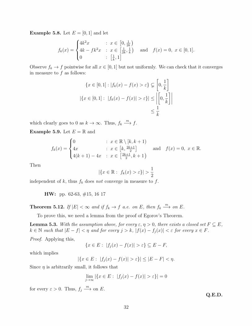
Example 5.8. Let E = [0, 1] and let

fk(x) =

4k2x : x ∈

[0, 1

2k

)4k − fk2x : x ∈

[12k, 1k

)0 :

[1k, 1] and f(x) = 0, x ∈ [0, 1].

Observe fk → f pointwise for all x ∈ [0, 1] but not uniformly. We can check that it convergesin measure to f as follows:

{x ∈ [0, 1] : |fk(x)− f(x) > ε} ([0,

1

k

]|{x ∈ [0, 1] : |fk(x)− f(x)| > ε}| ≤

∣∣∣∣[0, 1

k

]∣∣∣∣≤ 1

k

which clearly goes to 0 as k →∞. Thus, fkm−→ f .

Example 5.9. Let E = R and

fk(x) =

0 : x ∈ R \ [k, k + 1)

4x : x ∈[k, 2k+1

2

]4(k + 1)− 4x : x ∈

[2k+1

2, k + 1

) and f(x) = 0, x ∈ R.

Then

|{x ∈ R : fk(x) > ε}| > 1

2independent of k, thus fk does not converge in measure to f .

HW: pp. 62-63, #15, 16 17

Theorem 5.12. If |E| <∞ and if fk → f a.e. on E, then fkm−→ on E.

To prove this, we need a lemma from the proof of Egorov’s Theorem.

Lemma 5.3. With the assumption above, for every ε, η > 0, there exists a closed set F ⊆ E,k ∈ N such that |E − f | < η and for every j > k, |f(x)− fj(x)| < ε for every x ∈ F .

Proof. Applying this,{x ∈ E : |fj(x)− f(x)| > ε} ⊆ E − F,

which implies|{x ∈ E : |fj(x)− f(x)| > ε}| ≤ |E − F | < η.

Since η is arbitrarily small, it follows that

limj→∞|{x ∈ E : |fj(x)− f(x)| > ε}| = 0

for every ε > 0. Thus, fjm−→ on E.

Q.E.D.

32

Question: Is the converse of the theorem true?

Answer: No! Refer to the book for example. We are able to establish the followingweak converse, however.

Theorem 5.13. If fkm−→ on E, then there exists a subsequence {fkj}∞j=1 such that

limj→∞

fkj(x) = f(x) a.e.


6 Lebesgue Integration

Let E ∈ M(Rn), f : E → [0,∞] (measurable unless otherwise stated). We would like todefine

∫Ef , and since f is nonnegative,

∫Ef ∈ [0,∞].

Definition 6.1. Γ(f, E) is the graph of f over E, i.e., the set

{(x, f(x)

)∈ Rn+1 : x ∈ E, f(x) <∞}.

Example 6.1. Let f(x) = 1x

on [0, 1]. Then Γ(f) ={

(x, y) ∈ R2 : 0 < x ≤ 1, y = 1x

}.

Definition 6.2. R(f, E) is the region under the graph of f over E.

R(f, E) = {(x, xn+1) ∈ Rn+1 : x ∈ E, 0 ≤ xn+1 ≤ f(x) when it is finite

and 0 ≤ xn+1 <∞ otherwise}.

We will distinguish between M(Rn) and M(Rn+1). For outer measure and measure,|E|e(n) and |E∗|e(n+1), with |E|(n) and |E∗|(n+1), where E and E∗ are in Rn and Rn+1 respec-tively.

Definition 6.3.∫Ef = |R(f, E)|(n+1). Clearly R(f, E) ∈ M(R(n+1)) otherwise

∫Ef is not

defined.

Theorem 6.1. Let f ≥ 0 on E ∈ M(Rn). Then∫Ef exists if and only if f is measurable

on E.

Before proving the theorem, we first present a lemma.

Lemma 6.1. Let E ∈ M(Rn), a ∈ [0,∞]. Let fa = a on E (which is measurable). ThenR(fa, E) ∈M(Rn+1) and

∫Efa = a |E|(n).

Recall the convention is that 0 · x = 0 for all x ∈ [−∞,∞].

33

Proof. If |E|(n) = 0, we just need to show

|R(fa, E)|e(n+1) = 0,

which is left as an exercise.So assume |E|(n) > 0 and a <∞. If E is a (possibly) half-open interval, then R(f, E) =

E × [0, a] is another possibly half-open interval in Rn+1, thus R(f, E) ∈M(Rn+1 and∫E

fa = |R(f, E)|(n+1) = |E|(n) · |[0, a]|(1) = a · |E|(n) .

If E ⊆ Rn is open, then E =⋃∞k=1 Ik, a countable disjoint union of intervals. This says

R(fa, E) =∞⋃k=1

R(fa, Ik),

which is measurable as a countable union of measurable sets, so

|R(fa, E)|(n+1) =∞∑k=1

|R(fa, Ik)|(n+1) =∞∑k=1

a |Ik|(n) = a · |E| .

If E ⊆ Rn is of measure zero, we already have done it (as an exercise). Thus, if E ⊆ Rn,E ∈ M(Rn), |E| < ∞, then E = H − Z where |Z|(n) = 0 and H is a Gδ-set. Without loss

of generality, H =⋂∞i=1 Gi and G1 ⊇ G2 ⊇ · · · ⊇

⋂∞i=1Gi = H. Thus,

R(fa, E) =∞⋂i=1

R(fa, Gi)−R(fa, z).

We know R(fa, Gi) decreases since the G− i’s are nested with |R(fa, G1)|(n+1) = a · |G1|(n) <∞, which implies∣∣∣∣∣

∞⋂i=1

R(fa, Gi)

∣∣∣∣∣ = limi→∞|R(fa, Gi)| = lim

i→∞a · |Gi| = a |H| = a |E| .

If |E| = ∞, then we can write E =⋃∞k=1Ek with Ek = E ∩ (Bk(0) − Bk−1(0)) which is

measurable and finite, so we apply the previous step. Doing this, we get

R(fa, E) =∞⋃k=1

R(fa, Ek),

therefore, we have∫E

fa = |R(fa, E)| =∞∑k=1

|R(fa, Ek)| =∞∑k=1

a · |Ek| = a ·∞∑k=1

|Ek| = a · |E| .

It is left as an exercise to check the cases when a =∞ and 0 < |E| ≤ ∞.Q.E.D.

34

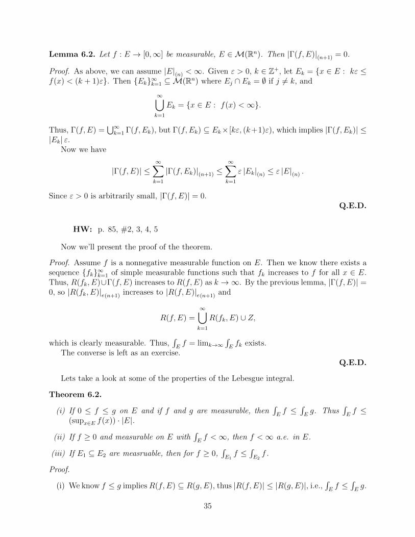
Lemma 6.2. Let f : E → [0,∞] be measurable, E ∈M(Rn). Then |Γ(f, E)|(n+1) = 0.

Proof. As above, we can assume |E|(n) <∞. Given ε > 0, k ∈ Z+, let Ek = {x ∈ E : kε ≤f(x) < (k + 1)ε}. Then {Ek}∞k=1 ⊆M(Rn) where Ej ∩ Ek = ∅ if j 6= k, and

∞⋃k=1

Ek = {x ∈ E : f(x) <∞}.

Thus, Γ(f, E) =⋃∞k=1 Γ(f, Ek), but Γ(f, Ek) ⊆ Ek× [kε, (k+1)ε), which implies |Γ(f, Ek)| ≤

|Ek| ε.Now we have

|Γ(f, E)| ≤∞∑k=1

|Γ(f, Ek)|(n+1) ≤∞∑k=1

ε |Ek|(n) ≤ ε |E|(n) .

Since ε > 0 is arbitrarily small, |Γ(f, E)| = 0.Q.E.D.

HW: p. 85, #2, 3, 4, 5

Now we’ll present the proof of the theorem.

Proof. Assume f is a nonnegative measurable function on E. Then we know there exists asequence {fk}∞k=1 of simple measurable functions such that fk increases to f for all x ∈ E.Thus, R(fk, E)∪Γ(f, E) increases to R(f, E) as k →∞. By the previous lemma, |Γ(f, E)| =0, so |R(fk, E)|e(n+1) increases to |R(f, E)|e(n+1) and

R(f, E) =∞⋃k=1

R(fk, E) ∪ Z,

which is clearly measurable. Thus,∫Ef = limk→∞

∫Efk exists.

The converse is left as an exercise.Q.E.D.

Lets take a look at some of the properties of the Lebesgue integral.

Theorem 6.2.

(i) If 0 ≤ f ≤ g on E and if f and g are measurable, then∫Ef ≤

∫Eg. Thus

∫Ef ≤

(supx∈E f(x)) · |E|.

(ii) If f ≥ 0 and measurable on E with∫Ef <∞, then f <∞ a.e. in E.

(iii) If E1 ⊆ E2 are measruable, then for f ≥ 0,∫E1f ≤

∫E2f .

Proof.

(i) We know f ≤ g impliesR(f, E) ⊆ R(g, E), thus |R(f, E)| ≤ |R(g, E)|, i.e.,∫Ef ≤

∫Eg.

35

(ii) We prove the contrapositive using the third condition. Suppose f = ∞ on a set ofpositive measure. Write E1 = {x ∈ E : f(x) =∞} ⊆ E, so the third condition implies∫

E1

f =∞|E| ≤∫E

f.

(iii) Observe E1 ⊆ E2 implies R(f, E1) ⊆ R(f, E2), thus∫E1f ≤

∫E2f .

Q.E.D.

Theorem 6.3 (Monotone Convergence Theorem). Let {fk}∞k=1 be a sequence of nonnegativemeasurable functions on E ∈ M. Assume fk increases to f for all x ∈ E, then

∫Efk

increases to∫Ef . In particular,

limk→∞

∫E

fk =

∫E

f.

Proof. The fact that{∫

Efk}∞k=1

increases follows from fk ≤ fk+1 and the previous theo-rem. R(fk, E) ∪ Γ(f, E) increases to R(f, E), which implies |R(fk+1, E)|(n+1) increases to|R(f, E)|(n+1).

Q.E.D.

Theorem 6.4. Suppose f ≥ 0 and measurable on E, and let E be partitioned into E =⋃∞k=1 Ek, Ek ∈M and Ek ∩ Ej = ∅ if k 6= j. Then∫

E

f =∞∑k=1

∫Ek

f.

Proof. R(f, E) =⋃∞k=1 R(fk, E), a disjoint union. This gives us |R(f, E)| =

∑∞k=1 |R(fk, E)|.

Q.E.D.

Theorem 6.5. Let f ≥ 0 be measurable on E ∈M. Then∫E

f = sup

{∞∑k=1

(infx∈Ek

f(x)

)|Ek|(n)

}where the supremum is over all countable partitions E =

⋃∞k=1Ek.


Corollary 6.1. If f ≥ 0 and |E| = 0, then∫Ef = 0.

Proof. They hypotheses imply the measurability of f . Then, for any partition of E, sayE =

⋃∞k=1Ek, then∫

E

f = sup

{∞∑k=1

(infx∈Ek

f(x)

)|Ek|(n)

}= sup{0} = 0.

Q.E.D.

36

Example 6.2. Let

f(x) =

{1 : x ∈ Q0 : x /∈ Q

.

(i) Let E = Q. Since |Q| = 0, we know∫Ef = 0.

(ii) In fact,∫R f =

∫Q f +

∫R−Q f = 0 + 0 = 0.

Theorem 6.6.

(i) If f and g are nonnegative measurable functions on E ∈ M, then if f(x) ≤ g(x) a.e.,then

∫Ef ≤

∫Eg.

(ii) If f(x) = g(x) a.e., then∫Ef =

∫Eg.

Proof. Clearly (ii) follows from (i). To prove (i), decompose E into sets {f > g} ∪ {f ≤g} = Z ∪ A, where |Z| = 0. Then∫

E

f =

∫Z

f +

∫A

f =

∫A

f ≤∫A

g =

∫A

g +

∫Z

g =

∫E

g.

Q.E.D.

Next, we will cover an important estimate/inequality, the Tchebyshev Inequality.

Theorem 6.7 (Tchebyshev’s Inequality). Let f ≥ 0 be measurable on E. Then, for everyα > 0 define

ωf,E(α) = ω(α) = |{x ∈ E : f(x) > α}| .

This is called the distribution function of f and satisfies

ωf,E(α) ≤ 1

α

∫E

f.

Remark 6.1. This gives a decay rate as α → ∞ and a “blow-up” rate as α → 0+. If∫Ef =∞, then the statement contains no information.

Example 6.3. Let E = Rn and f(x) = 1|x|p , where p > 0. Then

{x ∈ Rn :1

|x|p> α} =

{x ∈ Rn : |x| < α−

1p

}= B0

(α−

1p

).

Recall that |Br(x0)| = cnrn, where cn is a constant depending on the dimension. Thus,

ω(α) = cn(α−1p )n = cnα

−np .

This does not contradict Tchebyshev’s inequality since∫Rn f =∞. If we change E to B1(0),

then it turns out that ∫B1(0)

1

|x|p<∞

37

if and only if 0 < p < n. In that case, Tchebyshev’s inequality implies

ωf,B1(0)(α) ≤ 1

α

(∫B1(0)

1

|x|p

)<∞.

Tchebyshev’s inequality gives a weaker result than explicit calculation np> 1, so α−

np → 0

as α→∞ faster than α−1 does.

Proof. Fix α > 0. Let Eα = {x ∈ E : f(x) > α} ⊆ E, Eα ∈ M. On Eα, f(x) > α whichimplies

∫Ef ≥

∫Eαf by a previous theorem. But now∫

E

f ≥∫Eα

f ≥ α |Eα| = αω(α).

Thus, ω(α) ≤ 1α

∫Ef .

Q.E.D.

Theorem 6.8. Let f ≥ 0 on E, then f = 0 a.e. on E if and only if∫Ef = 0.

Proof. Suppose f = 0 a.e., then f ≤ 0 a.e., which implies

0 ≤∫E

f ≤∫E

0 = 0,

thus∫Ef = 0.

Conversely, if∫E

(f) = 0, apply Tchebyshev’s inequality for any α > 0. Then

|{x ∈ E : f(x) > α}| ≤ 1

α

∫E

f = 0.

Observe that {x ∈ E : f(x) 6= 0} =⋃∞k=1{x ∈ E : f(x) > 1

k}, which is a countable union

of sets of measure zero, thus it has measure zero. Hence, f = 0 a.e. on E.Q.E.D.

Theorem 6.9. If f ≥ 0 and c ∈ R+, then∫Ecf = c

∫Ef .

Proof. Recall if f is simple, f =∑N

i=1 aiχEi , then∫Ef =

∑Ni=1 ai |Ei| and cf =

∑Ni=1(cai)χEi ,

which implies ∫E

cf =N∑i=1

cai |Ei| = c

N∑i=1

ai |Ei| = c

∫E

f.

A general measurable f ≥ 0 can always be expressed as f = limk→∞ fk, with each fk ≥ 0simple, measurable, and increasing to f for all x ∈ E. Then it follows that cfk(x) increasesto c(f(x)). If we apply the monotone convergence theorem, we get that

∫Ef = limk→∞

∫Efk.

Thus, ∫E

cf = limk→∞

∫E

cfk = limk→∞

c

∫E

fk = c limk→∞

∫E

fk = c

∫E

f.

Q.E.D.

38

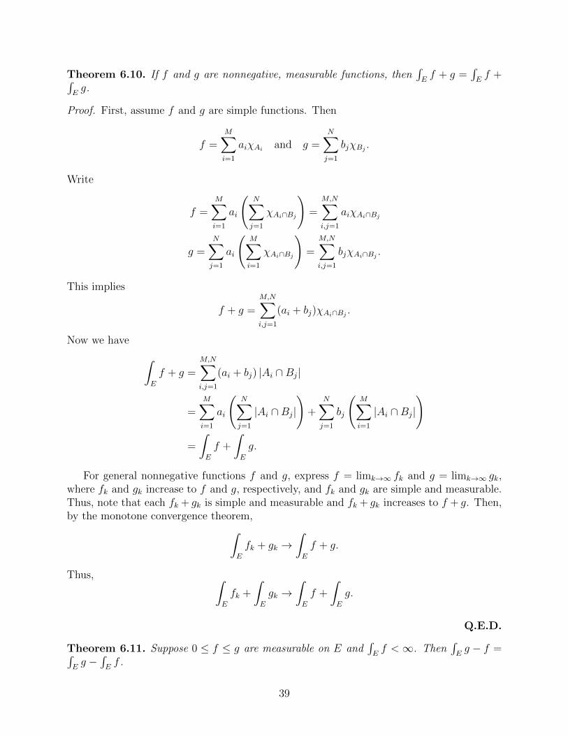
Theorem 6.10. If f and g are nonnegative, measurable functions, then∫Ef + g =

∫Ef +∫

Eg.

Proof. First, assume f and g are simple functions. Then

f =M∑i=1

aiχAi and g =N∑j=1

bjχBj .

Write

f =M∑i=1

ai

(N∑j=1

χAi∩Bj

)=

M,N∑i,j=1

aiχAi∩Bj

g =N∑j=1

ai

(M∑i=1

χAi∩Bj

)=

M,N∑i,j=1

bjχAi∩Bj .

This implies

f + g =

M,N∑i,j=1

(ai + bj)χAi∩Bj .

Now we have ∫E

f + g =

M,N∑i,j=1

(ai + bj) |Ai ∩Bj|

=M∑i=1

ai

(N∑j=1

|Ai ∩Bj|

)+

N∑j=1

bj

(M∑i=1

|Ai ∩Bj|

)

=

∫E

f +

∫E

g.

For general nonnegative functions f and g, express f = limk→∞ fk and g = limk→∞ gk,where fk and gk increase to f and g, respectively, and fk and gk are simple and measurable.Thus, note that each fk + gk is simple and measurable and fk + gk increases to f + g. Then,by the monotone convergence theorem,∫

E

fk + gk →∫E

f + g.

Thus, ∫E

fk +

∫E

gk →∫E

f +

∫E

g.

Q.E.D.

Theorem 6.11. Suppose 0 ≤ f ≤ g are measurable on E and∫Ef <∞. Then

∫Eg − f =∫

Eg −

∫Ef .

39

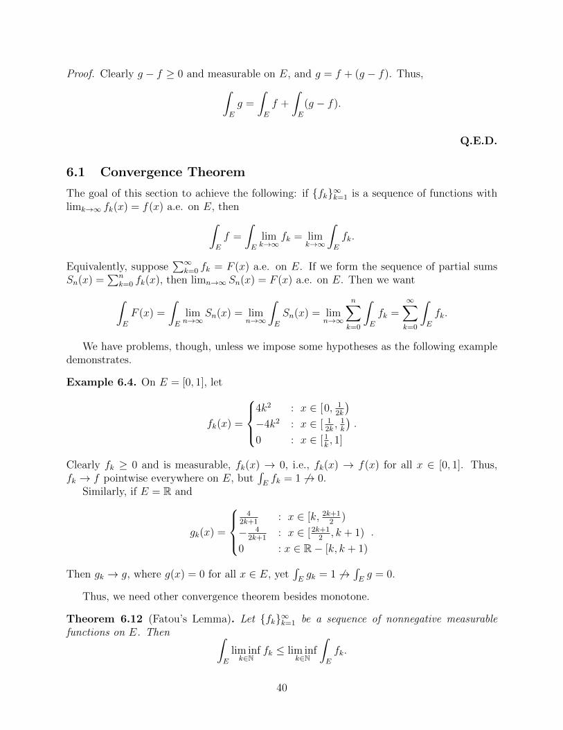
Proof. Clearly g − f ≥ 0 and measurable on E, and g = f + (g − f). Thus,∫E

g =

∫E

f +

∫E

(g − f).

Q.E.D.

6.1 Convergence Theorem

The goal of this section to achieve the following: if {fk}∞k=1 is a sequence of functions withlimk→∞ fk(x) = f(x) a.e. on E, then∫

E

f =

∫E

limk→∞

fk = limk→∞

∫E

fk.

Equivalently, suppose∑∞

k=0 fk = F (x) a.e. on E. If we form the sequence of partial sumsSn(x) =

∑nk=0 fk(x), then limn→∞ Sn(x) = F (x) a.e. on E. Then we want∫E

F (x) =

∫E

limn→∞

Sn(x) = limn→∞

∫E

Sn(x) = limn→∞

n∑k=0

∫E

fk =∞∑k=0

∫E

fk.

We have problems, though, unless we impose some hypotheses as the following exampledemonstrates.

Example 6.4. On E = [0, 1], let

fk(x) =

4k2 : x ∈ [0, 1

2k

)−4k2 : x ∈ [ 1

2k, 1k

)0 : x ∈ [ 1

k, 1]

.

Clearly fk ≥ 0 and is measurable, fk(x) → 0, i.e., fk(x) → f(x) for all x ∈ [0, 1]. Thus,fk → f pointwise everywhere on E, but

∫Efk = 1 6→ 0.

Similarly, if E = R and

gk(x) =

4

2k+1: x ∈ [k, 2k+1

2)

− 42k+1

: x ∈ [2k+12, k + 1)

0 : x ∈ R− [k, k + 1)

.

Then gk → g, where g(x) = 0 for all x ∈ E, yet∫Egk = 1 6→

∫Eg = 0.

Thus, we need other convergence theorem besides monotone.

Theorem 6.12 (Fatou’s Lemma). Let {fk}∞k=1 be a sequence of nonnegative measurablefunctions on E. Then ∫

E

lim infk∈N

fk ≤ lim infk∈N

∫E

fk.

40

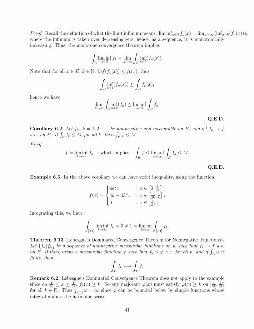
Proof. Recall the definition of what the limit infimum means: lim infk∈N fk(x) = limk→∞ (infn≥k(fn(x))),where the infimum is taken over decreasing sets, hence, as a sequence, it is monotonicallyincreasing. Thus, the monotone convergence theorem implies∫

E

lim infk∈N

fk = limk→∞

∫E

infn≥k

(fn(x)).

Note that for all x ∈ E, k ∈ N, inf(fk(x)) ≤ fk(x), thus∫E

infn>k

(fn(x)) ≤∫E

fk(x),

hence we have

limk→∞

∫E

infn>k

(fn) ≤ lim infk∈N

∫E

fk.

Q.E.D.

Corollary 6.2. Let fk, k = 1, 2, . . ., be nonnegative and measurable on E, and let fk → fa.e. on E. If

∫Efk ≤M for all k, then

∫Ef ≤M .

Proof.

f = lim infk→∞

fk, which implies

∫E

f ≤ lim infk→∞

∫E

fk ≤M.

Q.E.D.

Example 6.5. In the above corollary we can have strict inequality, using the function

f(x) =

4k2x : x ∈

[0, 1

2k

]4k − 4k2x : x ∈

[12k, 1k

]0 : x ∈

[1k, 1] .

Integrating this, we have ∫[0,1]

lim infk→∞

fk = 0 6= 1 = lim infk→∞

∫[0,1]

fk.

Theorem 6.13 (Lebesgue’s Dominated Convergence Theorem for Nonnegative Functions).Let {fk}∞k=1 be a sequence of nonnegative measurable functions on E such that fk → f a.e.on E. If there exists a measurable function ϕ such that fk ≤ ϕ a.e. for all k, and if

∫Eϕ is

finite, then ∫E

fk −→∫E

f.

Remark 6.2. Lebesgue’s Dominated Convergence Theorem does not apply to the examplesince on 1

4k≤ x ≤ 1

3k, fk(x) ≥ k. So any majorant ϕ(x) must satisfy ϕ(x) ≥ k on [ 1

4k, 1

3k]

for all k ∈ N. Thus∫

[0,1]ϕ = ∞ since ϕ can be bounded below by simple functions whose

integral mimics the harmonic series.

41

Proof. One inequality follows immediately from Fatou’s Lemma:∫E

f ≤ lim infk→∞

∫E

fk.

So, it suffices to show

lim supk→∞

∫E

fk ≤∫E

f.

Let gk = ϕ− fk, and notice gk ≥ 0 a.e. on E and limk→∞ gk = ϕ− limk→∞ fk = ϕ− f . Now,Fatou’s Lemma implies ∫

E

ϕ− f =

∫E

limk→∞

gk

≤ lim infk→∞

∫E

gk

= lim infk→∞

∫E

ϕ− fk

= lim infk→∞

[∫E

ϕ−∫E

fk

]=

∫E

ϕ− lim supk→∞

∫E

fk.

On the other hand, ∫E

ϕ− f =

∫E

ϕ−∫E

f.

Combining these two inequalities and cancelling∫Eϕ, we achieve the desired result.

Q.E.D.

Definition 6.4. If at least one of the integrals∫Ef+ or

∫Ef− is finite, then

∫Ef is defined

to be∫Ef+ −

∫Ef−. If

∫Ef exists and is finite, we say that f is Lebesgue integrable, or

simply integrable, on E and write f ∈ L(E). Thus,

L(E) = L1(E) = L1(E, dx) = {f :

∫E

f <∞},

where dx represents Lebesgue measure. Observe that L1(E) is a vector space under pointwiseaddition and multiplication.

Observe that∣∣∣∣∫E

f

∣∣∣∣ =

∣∣∣∣∫E

f+ −∫E

f−∣∣∣∣ ≤ ∣∣intEf+

∣∣+

∣∣∣∣∫E

f−∣∣∣∣ =

∫E

f+ +

∫E

f− =

∫E

|f | .

Definition 6.5. A function f is essentially bounded if there exists M < ∞ such that|f(x)| ≤ M for almost every x ∈ E. The essential supremum is then defined to be theinfimum of the M ’s that satisfy this property.

42

Proposition 6.1. Let |E| <∞. Then if f is essentially bounded,∣∣∣∣∫E

f

∣∣∣∣ ≤ ess supx∈E

|f | · |E| .

Proof. ∣∣∣∣∫E

f

∣∣∣∣ ≤ ∫E

|f |

≤∫E

ess supx∈E

|f |

= ess supx∈E

|f |∫E

1

= ess supx∈E

|f | · |E| .

Q.E.D.

Theorem 6.14. Let f : E → R be measurable on E. Then f is integrable over E if andonly if |f | is integrable over E.

Proof. If |f | ∈ L1(E), use the inequality above to get f ∈ L1(E). Conversely, if f ∈ L1(E),then

∫Ef+ and

∫Ef− both must be finite. Then∫

E

|f | =∫E

f= + f− =

∫E

f+ +

∫E

f− <∞.

Thus, |f | ∈ L1(E) by definition.Q.E.D.

Many of the results for nonnegative extended real-valued functions extend to R-valuedfunction if either

∫Ef is defined or f ∈ L1(E). As a warning, however, the integral operator

is no longer monotonic in the sets we integrate over (simply consider the function f(x) = 2xover the intervals [−1, 1] and [0, 1]).We do however, have the following proposition.

Proposition 6.2. Let f ∈ L1(E) and E2 ⊆ E1. Then f∣∣E2∈ L1(E2) and∫

E2

|f | ≤∫E1

|f |.

Theorem 6.15. If f ∈ L(E), then f is finite a.e. in E.


Theorem 6.16.

(i) If both∫Ef and

∫Eg exist and if f ≤ g a.e. in E, then

∫Ef ≤

∫Eg. In particular, if

f = g a.e. in E, then∫Ef =

∫Eg.

43

(ii) If∫E2f exists and E1 is a measurable subset of E2, then

∫E1f exists.


Theorem 6.17. If∫Ef exists and E =

⋃∞k=1Ek is the countable union of disjoint measurable

sets Ek, then ∫E

f =∞∑k=1

∫Ek

f.


Theorem 6.18. If |E| = 0 or if f = 0 a.e. in E, then∫Ef = 0.


6.2 Linearity of the Integral

Lemma 6.3. If∫Ef exists and c ∈ R, then

∫Ecf exists and equals c

∫Ef .

Proof. Suppose c = −1. Then∫Ef exists implies

∫Ef =

∫Ef+ −

∫Ef− with at least one of

the integrals on the right finite. Note that (−f)+ = f− and (−f)− = f+. Then∫E

(−f) =

∫E

(−f)+ −∫E

(−f)−

=

∫E

f− −∫E

f+

= −(∫

E

f+ −∫E

f−)

= −∫E

f.

Now, suppose 0 ≤ c <∞. Then∫E

cf =

∫E

(cf)+ −∫E

(cf)−

=

∫E

cf+ −∫E

cf−

= c

∫E

f+ − c∫E

f−

= c

(∫E

f+ −∫E

f−)

= c

∫E

f.

For general c ∈ R, either c ≥ 0 or −c ≥ 0. In the latter case, c = −c′, thus apply case 2or cases 2 and 1 respectively.

Q.E.D.

44

Corollary 6.3. If∫E1f1 and

∫E2f2 are defined and c1, c2 ∈ R, then∫

E1

c1f1 +

∫E2

c2f2 = c1

∫E1

f1 + c2

∫E2

f2.

Thus, the set of function f such that∫Ef is defined is a vector space over R as is L1(E).

HW: Chap. 5, #7,8,9,11

Theorem 6.19. If f, g ∈ L1(E), then f +G ∈ L1(E) and∫Ef + g =

∫E

+∫Eg.


Thus, L1(E) is a vector space over R. In fact, L1(E) is a normed linear space with

‖f‖L1(E) =

∫E

|f |,

which satisfies

(i) ‖f‖L1(E) ≥ 0 with equality if and only if f = 0 a.e. on E;

(ii) ‖cf‖L1(E) = |c|‖f‖L1(E);

(iii) ‖f + g‖L1(E) ≤ ‖f‖L1(E) + ‖g‖L1(E).

Strictly speaking, we need to consider

Z(E) = {f : f = 0 a.e. on E}.

Clearly this is a linear subspace of L1(E), so we replace L1(E)/Z(E) to identify all of thefunctions with 0. Now L1(E) becomes a metric space, where

d(f, g) = ‖f − g‖L1(E).

Example 6.6. fk −→ f in L1(E) if d(fk, f) =∫E|fk − f | −→ 0 as k →∞.

Definition 6.6. If (X, ‖ · ‖) is a normed linear space, then a linear functional λ : X → Ris bounded (or continuous) if there is some constant C <∞ such that λ(v) ≤ C · ‖v‖.

We know that if f ∈ L1(E), then λ(f) =∫Ef is a linear function on L1(E) and

|λ(f)| =∣∣∣∣∫E

f

∣∣∣∣ ≤ ∫E

|f | = 1 · ‖f‖L1(E),

which implies λ is a bounded linear functional with constant C = 1.

Theorem 6.20. Suppose f ∈ L1(E) and g : E → R is measurable. Then

45

(i) if there exists M < ∞ such that |g(x)| ≤ Mf(x), then g ∈ L1(E) with ‖g‖L1(E) ≤M‖f‖L1(E);

(ii) if there exists constant a and b such that af(x) ≤ g(x) ≤ bf(x) a.e. on E, then

a

∫E

f ≤∫E

g ≤ b

∫E

f,

so g ∈ L1(E).

If m(x) is essentially bounded on E, then f ∈ L1(E) implies

fλm−→ λm(f) =

∫E

m(x)f(x)dx.

Observe λm(cf) = cλm(f) for all c ∈ R and f ∈ L1(E). Also, λm(f + g) ≤ λm(f) + λm(g)for all f and g ∈ L1(E), thus λm is a linear functional.

By the theorem,

|λm(x)| ≤∫E

|m(x)f(x)|dx ≤M

∫E

|f | = M‖f‖L1(E)

for any M for which M ≥ ess supx∈E |m(x)|. In fact, here λm is a bounded linear functionwith constant C = ess supx∈E |m|. Furthermore, every bounded linear functional on L1(E)arises in this way.

6.3 Convergence Theorems for General Functions

Theorem 6.21 (Monotone Convergence Theorem). Let {fk}∞k=1 be a sequence of measurablefunctions on E. If fk monotonically converges to f a.e. and there exists ϕ ∈ L1(E) suchthat fk(x) ≥ ϕ(x) a.e. on E, then limk→∞

∫Efk =

∫Ef .

Proof. Clearly fk(x)− ϕ(x) ≥ 0 e.e on E and fk(x)− ϕ(x) increases to f(x)− ϕ(x) a.e. onE. The monotone convergence theorem for nonnegative functions imply∫

E

fk − ϕ −→∫E

f − ϕ,

but that means ∫E

fk −∫E

ϕ −→∫E

f −∫E

ϕ.

Cancelling the∫Eϕ from both sides yields the desired result.

Q.E.D.

Theorem 6.22 (Fatou’s Lemma). Let {fk}∞k=1 be a sequence of functions on E such thatthere exists ϕ ∈ L1(E) with fk ≥ ϕ a.e. on E. Then∫

E

lim infk→∞

fk ≤ lim infk→∞

∫E

fk.

46

Proof. Apply Fatou’s Lemma for nonnegative functions to {fk − ϕ}∞k=1, using

lim infk→∞

(fk − ϕ) = lim infk→∞

(fk)− ϕ,

so∫Efk − ϕ =

∫Efk −

∫Eϕ implies∫

E

lim infk→∞

fk −∫E

ϕ =

∫E

lim infk→∞

(fk)− ϕ ≤ lim infk→∞

[∫E

fk −∫E

ϕ

]= lim inf

k→∞

∫E

fk −∫E

ϕ.

Cancelling the∫Eϕ from both sides yields Fatou’s Lemma for arbitrary measurable f .

Q.E.D.

Theorem 6.23 (Lebesgue’s Dominated Convergence Theorem). If {fk}∞k=1 is a sequence ofmeasurable functions on E, ϕ ∈ L1(E) such that |fk(x)| ≤ ϕ(x), and fk(x) −→ f(x) a.e. onE, then

limk→∞

∫E

fk =

∫E

f(x).

Proof. For a.e. x ∈ E, −ϕ(x) ≤ fk(x) ≤ ϕ(x), so 0 ≤ fk(x) + ϕ(x) ≤ 2ϕ(x). Observe2ϕ ∈ L1(E), thus

fk(x) + ϕ(x) −→ f(x) + ϕ(x) a.e. x ∈ E,so we can apply Lebesgue’s Dominated Convergence Theorem for nonnegative functions.Hence, ∫

E

fk +

∫E

ϕ =

∫E

fk + ϕ −→∫E

f + ϕ =

∫E

f +

∫E

ϕ.

Thus, limk→∞∫Efk =

∫Ef .

Q.E.D.

6.4 The Distribution Function and Lp-spaces

For measurable f : E → R, we defined ω for every α ∈ R in the following way,

ωf,E(α) = ωf (α) = ω(α) = |{x ∈ E : f(x) > α}| .

Thus, ω : R→ [0,∞]. If |E| <∞, then ω : R→ [0,∞).Let us review some elementary facts regarding ω.

(i) If α ≤ β, then ω(α) ≥ ω(β), i.e., ω is a decreasing function;

(ii) if f = f a.e. on E, then ωf = ωf .

As α → ∞, {f > α} −→ {f = ∞}, which implies limα→∞ ω(α) = |{f =∞}|. It isconvenient to assume |{f =∞}| = 0, which holds if and only if limα→∞ ω(α) = 0. Also noteas limα→−∞ ω(α) = |{f > −∞}|. Similar to before, it is convenient to assume |{f = −∞}| =0, thus limα→−∞ ω(α) = |E|.

Lemma 6.4. If α < β, then

ω(α)− ω(β) = |{α < f(x) ≤ β}| .

47

Proof.

ω(α)− ω(β) = |{f > α}| − |{f > β}|= |{f > β} ∪ {β ≥ f > α}| − |{f > β}|= |{f > β}|+ |{β ≥ f > α}| − |{f > β}|= |{β ≥ f > α}| .

Q.E.D.

Lemma 6.5. For every α ∈ R,

(i) ω is continuous from the right: ω(α) = limε→0+ ω(α + ε);

(ii) limε→0− ω(α + ε) = |{f ≥ α}|;

(iii) ω is continuous at alpha if and only if |{f = α}| = 0.

Proof. For any sequence εk → 0+, {f > α + εk} increases to {f > α}, thus ω(α + εk)increases to ω(α). On the other hand, {f > α − εk} decreases to {f ≥ α}, which impliesω(α− εk) decreases to |{f ≥ α}|. Note that ω(·) is constant on some open interval (α, β) ifand only if f(x) /∈ (α, β] a.e.

Q.E.D.

Example 6.7. We will show that it is necessary to take the set E with finite measure. Takef(x) = e−x. Then ω(α) = 0 for all α ≥ 0 while ω(α) = ∞ for any α < 0. In particular,ω(0−) =∞ 6= 0 = |{f ≥ 0}|.

Proof. Let εk → 0+, thenω(α− εk) = |{f > α− εk}| .

Thus∞⋂k=1

{x : f(x) > α− εk} = {x : f(x) ≥ α}.

Q.E.D.

To get the convergence of measure, we need |E| <∞.

Proposition 6.3. ω is continuous at α if and only if |{f = α}| = 0.

Definition 6.7. We say f and g are equimeasurable or equidistributed on E if

ωf,E(α) = ωg,E(α)

for all α ∈ R. This will imply that∫Eϕ(f) =

∫Eϕ(g) for all continuous ϕ.

There is a natural relation between the Lebesgue integral of f and Riemann-Stieltjesintegral of ωf .

48

Theorem 6.24. Suppose −∞ < a < b < ∞ and a < f(x) ≤ b a.e. in E is measurable.Then ∫

E

f = −∫ b

a

αdωf,E(α).

Proof. Let f be a bounded function, |E| <∞ so that∫Ef is defined and∣∣∣∣∫

E

f

∣∣∣∣ ≤ ess supx∈E

|f | · |E| <∞,

thus f ∈ L1(E). Note that ϕ(α) is continuous on [a, b] and ωf,E is a function of boundedvariation since it is decreasing and bounded. Thus∫ b

a

αdωf,E(α)

is defined as a Riemann-Stieltjes integral.Let

Γ = {a = α0 < α1 < · · · < αn = b}

be a partition of [a, b] (the range). For each 1 ≤ j ≤ k, define

Ej = {x ∈ E : αj−1 < f(x) ≤ αj}.

Then E =⋃kj=1Ej (up to a set of measure zero). The pairwise disjointness implies

∫E

f =k∑j=1

∫Ej

f.

Note that ∫Ej

αj−1 <

∫Ej

f ≤∫Ej

αj,

that is,

αj−1 |Ej| <∫Ej

f ≤ αj |Ej| .

Thus,k∑j=1

αj−1 |Ej| <∫E

f ≤k∑j=1

αj |Ej| .

Observe that

|Ej| = |{αj−1 < f(x) ≤ αj}| = ω(αj−1)− ω(αj) = −[ω(αj)− ω(αj−1)].

Inserting this into the left-hand side and the right-hand side, we get two Riemann-Stieltjessums for −

∫ baαdω(α). Letting |Γ| → 0, the left-hand side and the right-hand side approach

−∫ baαdω(α), forcing

∫Ef = −

∫ baαdω(α).

Q.E.D.

49

In fact, the next theorem shows we can relax the bounded assumption.

Theorem 6.25. Let f : E → R be measurable. For −∞ < a < b < ∞, let Eab = {x ∈ E :a < f(x) < b}. Then ∫

Eab

f = −∫ b

a

αdωf,E(α).

Theorem 6.26. Let f : E → R be measurable. If either of∫E

f or

∫ ∞−∞

αdωf,E(α)

exists and is finite, then the same is true for the other and∫E

f = −∫ ∞−∞

αdω(α).


Corollary 6.4. If f and g are equimeasurable on E, then f ∈ L1(E) if and only if g ∈ L1(E)and

∫Ef =

∫Eg.

Proof. ∫E

f = −∫ ∞−∞

αdωf,E(α) = −∫ ∞−∞

αdωg,E(α) =

∫E

g.

Q.E.D.

Theorem 6.27. Let ϕ : R→ R is continuous and f : E → R is measurable. Then∫E

ϕ(f) = −∫ ∞−∞

ϕ(α)dωf,E(α).

If f ≥ 0, then ∫E

ϕ(f) = −∫ ∞

0

ϕ(α)dωf,E(α).

For general f , replace f by |f |. This gives us∫E

ϕ(|f |) = −∫ ∞

0

ϕ(α)dω|f |,E(α).

Example 6.8. Consider ϕ(α) = αp where 0 < p <∞ is fixed. Then∫E

|f(x)|p = −∫ ∞−∞

αpdωf,E(α).

Definition 6.8. We define the Lp-spaces as follows:

Lp(E) =

{f :

∫E

|f |p <∞}.

50

When p = 1, these are just the integrable functions on E. When p = 2, these are thesquare-integrable functions on E. Likewise, we can let p = ∞ and we get the essentiallybounded functions on E.

For 1 ≤ p <∞ define the Lp-norm of f ∈ Lp(E) to be

‖f‖Lp(E) = ‖f‖Lp = ‖f‖p =

(∫E

|f |p) 1

p

.

For p =∞, ‖f‖L∞(E) = ess supx∈E |f |.

Theorem 6.28. (Lp(E), ‖ · ‖p) is a normed linear space (and thus a metric space withdLp(f, g) = ‖f − g‖Lp).

Theorem 6.29 (Tchebyshev’s Inequality). For p = 1, we have ωf,E ≤ 1α

∫Ef , with f ∈

L1(E). When 0 < p <∞,

ω|f |,E(α) ≤ α−p∫E

|f |p.

Note 6.1. For f ≥ 0, an estimate of the form

ωf (α) ≤ C

α

p

does not imply f ∈ Lp(E).

Example 6.9. Take E = R and f(x) = 1|x| . Then

|{x ∈ R : f(x) > α}| =∣∣∣∣{ 1

|x|> α}

∣∣∣∣ =

∣∣∣∣{|x| < 1

α}∣∣∣∣ =

2

α,

but ∫R

1

|x|=∞.

Even on the bounded set E = [−1, 1] the function f /∈ Lp(E).

Definition 6.9. We say that f is in weak-Lp if there exists C <∞ such that

ω|f |,E(α) ≤ C

αp, 0 < α <∞.

The notation for weak-Lp is Lpweak = Lpw.

Note that f > α on Eα implies f > αχEα on Eα, thus fp > αpχEα , which implies∫Eα

fp ≥ αp |Eα| ,

i.e.,

|{x : f > α}| ≤ 1

αp

∫Eα

≤ 1

αp

∫E

fp.

51

This then implies

|{x : |f | > α}| ≤ 1

αp

∫{|f |>α}

|f |p ≤∫E

|f |p.

These are the Lp Tchebyshev inequalities. Thus, αpωf (α) ≤∫Efp <∞ if fp is integrable,

and thus f ∈ Lp(E). Hence, αpω(α) is bounded on (0,∞).

Question: Is this a sufficient condition for f ∈ Lp(E)?

Answer: No, there are other necessary conditions.

Since |E| < ∞, αpω(α) = αp |Eα| −→ 0 as α → 0+. We can show αpω(α) −→ 0 asα→∞, so it suffices to show

∫Eαfp −→ 0 as α→∞.

Lemma 6.6. If f ∈ Lp(E), then

limα→∞

αpω(α) = 0.

Proof. We will do this by using Tchebyshev. It suffices to show for every {αk}∞k=1 ⊆ (0,∞),αk →∞ as k →∞ that

∫Eαk

fp → 0. Since∫Efp <∞, f is finite a.e. Thus, let

fk(x) =

{f(x) : x ∈ Eαk0 : x ∈ E − Eαk

.

Now, clearlylimk→∞

fk(x) = 0 a.e.

Also, 0 ≤ (fk(x))p ≤ (f(x))p. Since f ∈ Lp(E), the Lebesgue Dominated ConvergenceTheorem implies

limk→∞

∫E

fpk =

∫E

limk→∞

fpk = 0.

Thus, we have

limk→∞

∫Eαk

fpk = 0,

as desired.Q.E.D.

Theorem 6.30. If |E| < ∞, 0 < p < ∞, f ∈ Lp(E) is nonnegative, then αpωf,E(α) is abounded function on (0,∞) and tends to 0 as α→ 0+ or α→∞.

Again, the conclusion is not sufficient for f ∈ Lp(E).

Theorem 6.31. Let f be a nonnegative function over a set with finite measure, and let∫Efp <∞. Then ∫

E

fp = −∫ ∞

0

αpdωf,E(α) = p

∫ ∞0

αp−1ω(α)dα.

52

Proof. For 0 < a < b <∞,

−∫ b

a

αpdω(α) = −αpω(α)

∣∣∣∣ba

+

∫ b

a

ω(α)pαp−1dα,

by integration by parts. Now, this is

−bpω(b) + apω(a) +

∫ b

a

ω(α)pαp−1dα.

Now, from the lemma above, we can reduce the first two terms to 0 as a→ 0+ and b→∞respectively. Thus, we have the desired result.

Q.E.D.

Unfortunately, this still is not enough in order to guarantee f ∈ Lp(E).

7 Lp Space

In analysis, 1 ≤ p ≤ ∞, the Lp spaces are basic examples of complete normed linear spaces,also known as Banach spaces. For 0 < p < 1, Lp is not normed but is a topological vectorspace.

Definition 7.1. Let E be a measurable subset of Rn, 0 < p < ∞. We say that f ∈ Lp(E)if∫E|f |p <∞. The norm associated with 1 ≤ p <∞ is

‖f‖Lp =

(∫E

|f |p) 1

p

.

For p =∞,L∞(E) = {f : ess sup

x∈E|f | <∞}.

The natural norm on this set is to take the essential supremum.

Thus, ω(ess supx∈E |f |) = 0 and for all α ≥ ess sup |f |. For every α < ess sup |f |, ω|f |(α) >0.

Theorem 7.1. For 1 ≤ p ≤ ∞, (Lp(E), ‖ · ‖Lp) is a normed linear space, thus Lp(E) is avector space with respect to pointwise linear combinations.

Recall that a norm satisfies the properties of a metric, so strictly speaking, we need toreplace Lp(E) by Lp(E)/Z(E), where Z(E) is the subspace of functions equal to 0 a.e.

Theorem 7.2. If |E| <∞ and f ∈ Lp(E) for all p ≥ p0 for some fixed p0, then

limp→∞‖f‖Lp = ‖f‖L∞ .

53

Proof. Let M = ‖f‖L∞ = ess sup |f |. For any M < M , we have that

A = {x ∈ E : |f(x)| > M}

has the property that |A| > 0. Then,

‖f‖Lp(E) ≥ ‖f‖Lp(A) =

(∫A

|f |p) 1

p

> M |A|1p .

As p→∞, we have lim infp→∞ ‖f‖Lp ≥ M .On the other hand, |f | ≤M a.e. on E, which implies

‖f‖Lp =

(∫E

|f |p) 1

p

≤(∫

E

Mp

) 1p

= M |E|1p ,

which clearly converges to M as p→∞. Thus,

lim supx∈E

‖f‖Lp ≤M.

Thus the limit exists as p→∞, and the common value is ‖f‖L∞ .Q.E.D.

Observe that most inequalities are trivial if |E| = 0, so we will always assume |E| > 0.Suppose E2 ⊆ E. Then if f ∈ Lp(E), f

∣∣E2∈ Lp(E2). This implies ‖f‖Lp(E2) ≤ ‖f‖Lp(E1).

Thus note that the operator RE,E2 which sends f to f∣∣E2

is a bounded linear operator with

‖RE,E2‖ = 1.

Theorem 7.3.

(i) Let 0 < p2 < p1 ≤ ∞ with |E| < ∞. Then f ∈ Lp1(E) implies f ∈ Lp2(E). Hence,there is a natural inclusion Lp1(E) ↪→ Lp2(E), and so the Lp-spaces shrink as p in-creases.

(ii) If 1 ≤ p2 < p1 ≤ ∞, then the inclusion above is a bounded linear operator.

We will prove the first part now, saving the proof for the second part until after moreestimates have been established.

Proof. Decompose

E = E1 ∪ E2 = {x ∈ E : |f(x)| ≤ 1} ∪ {x ∈ E : |f(x)| > 1}

into disjoint measurable subsets.First, notice that when x ∈ E1, |f |p2 ≤ 1, so

∫E1|f |p2 ≤ |E1| ≤ |E| < ∞. Next, use the

fact that for every x ∈ E2, |f(x)|p is increasing for 0 < p <∞. Thus,∫E2

|f |p2 ≤∫E2

|f |p1 ≤∫E

|f |p1 .

54

Hence, ∫E

|f |p2 ≤ |E|+∫E

|f |p1 <∞.

This follows from the fact that |E| <∞ and f ∈ Lp1(E).Q.E.D.

Example 7.1. Note that this is not true in general if |E| =∞. Take E = R and let p2 < p1.Then neither containment holds. To see this, pick q ∈ (p2, p1) and note that p2

q< 1 < p1

q.

Letf(x) = |x|−

1q · χ{|x|≤1}.

Thus f ∈ Lp2 − Lp1 .On the other hand, let

g(x) = (1 + |x|)−1q .

Then g ∈ Lp1 − Lp2 .

7.1 Some Inequalities

Theorem 7.4 (Young’s Inequality). Let ϕ : [0,∞) → [0,∞) be continuous, strictly in-creasing, ϕ(0) = 0. Let ψ = ϕ−1, which exists since ϕ is strictly increasing. Then, for alla, b ∈ (0,∞), we have

ab ≤∫ a

0

ϕ(x)dx+

∫ b

0

ψ(y)dy,

with equality if and only if ϕ(a) = b.

Example 7.2. Take ϕ(x) = xα, 0 < α <∞ so that ψ(y) = y1α . Young’s Inequality implies

ab ≤∫ a

0

xαdx+

∫ b

0

y1αdy.

Integration yields

ab ≤ aα+1

α + 1+

b1α

+1

1α

+ 1.

Let p = α + 1 so 1 < p < ∞. Note that 1α

+ 1 = p′ = pp−1

. Thus, p + p′ = 1, and hence p′

maps (0,∞) back into itself (called an involution), and we can check (p′)′ = p. Note thatp = p′ if and only if p = p′ = 2, and we have 1 < p < 2 implies p′ ∈ (2,∞) vice versa.

In this special case, Young’s inequality becomes

ab ≤ ap

p+bp′

p′,

with 0 < a, 0 < b, 1 < p <∞, 1 < p′ <∞, and 1p

+ 1p′

= 1.

55

Theorem 7.5 (Holder’s Inequality). If 1 ≤ p ≤ ∞ and f and g are measurable functionson E, then ∫

E

|fg| ≤ ‖f‖Lp(E) · ‖g‖Lp′ (E),

where we define 1′ =∞ and ∞′ = 1.

When p = p′ = 2, this is known as the Cauchy-Schwarz Inequality.

Proof. If ‖f‖Lp(E) = ∞ or ‖g‖Lp′ (E) = ∞, then there is nothing to prove, so assume‖f‖Lp(E), ‖g‖Lp′ (E) <∞. Likewise, the result follows trivially if ‖f‖Lp(E) = 0 or ‖g‖Lp′ (E) =0, as then f = 0 a.e. or g = 0 a.e., and so |fg| = 0 a.e., so the inequality effectively says0 ≤ 0.

If p = 1 and p′ =∞, then |g(x)| ≤ ‖g‖L∞(E) = ess supx∈E |g(x)|. Thus

|f(x)g(x)| ≤ ‖g‖L∞(E)|f(x)|,

and so‖fg‖L1(E) ≤ ‖g‖L∞(E) · ‖f‖L1(E),

as desired. Obviously if we switch the roles of p and p′ we can form a similar argumentshowing the claim is true for that case.

Now, to prove H older’s Inequality for p, p′ ∈ (0,∞), it suffices to do it under theassumption that ‖f‖Lp(E) = ‖g‖Lp′ (E) = 1. This is clear if we consider

f(x) =f(x)

‖f‖Lp,

which implies

‖f‖Lp =1

‖f‖Lp· ‖f‖Lp = 1,

and similarly for g. Thus, assuming the claim to be true for normalized functions for themoment, we have ∫

E

∣∣∣f g∣∣∣ ≤ ‖f‖Lp‖g‖Lp′ = 1.

Now, using the definition of f and g, we have∫E

|fg| ≤ ‖f‖Lp · ‖g‖Lp′ .

Thus, we need only prove the claim for normalized functions. Using Young’s Inequality, wehave

|f(x)g(x)| ≤ |f(x)|p

p+|g(x)|p′

p′,

so that by the linearity of the Lebesgue integral, we have∫E

|fg| ≤ 1

p

∫E

|f |p +1

p′

∫E

|g|p′ =1

p+

1

p′= 1

56

since ∫E

|f |p =

((∫E

|f |p) 1

p

)p

= ‖f‖pp = 1.

Clearly a similar argument holds for g. Thus the claim has been proven.Q.E.D.

Example 7.3. As an application of Hoder’s Inequality, we can now prove the second claimfrom the theorem above.

Proof. Recall we want to show that |E| <∞ and p2 < p1 implies Lp1(E) ⊆ Lp2(E). To thatend, the inclusion Lp1(E) ↪→ Lp2(E) is a bounded linear operator.∫

E

|f |p2 =

∫E1

|f |p2 +

∫E2

|f |p2 .

Now, ∫E2

|f |p2 ≤ 1 ·∫E

|f |p1quad and

∫E1

|f |p2 = 1 ·∫E1

|f |p2 .

Pick p > 1 so that p2p = p1. Then∫E1

|f |p2 · 1 ≤ ‖|f |p2‖p · ‖1‖p′ = ‖|f |p2‖p · |E1|1p ≤ ‖|f |p2‖p |E|

1p .

Now,

‖|f |p2‖p =

(∫E1

|f |p2p) 1

p

≤ ‖f‖p2p1p1 .

Now we can add, take the 1p2

power, and we get

‖f‖p2 ≤ C · ‖f‖p1 ,

which implies the inclusion.Q.E.D.

Theorem 7.6 (Minkowski’s Inequality). Let 1 ≤ p ≤ ∞, and let f and g measurablefunctions finite a.e. on a set E. Then

‖f + g‖p ≤ ‖f‖p + ‖g‖p.

Proof. We’ll handle this by cases. First, suppose p =∞. Then, by definition, |f(x)| ≤ ‖f‖∞a.e. and |g(x)| ≤ ‖g‖∞ a.e. The triangle inequality implies that

|f(x) + g(x)| ≤ ‖f‖∞ + ‖g‖∞.

Since ‖f‖∞ + ‖g‖∞ is an upper bound a.e., it is at least as great as the least upper bounda.e., hence

ess supx∈E

|f(x) + g(x)| = ‖f + g‖∞ ≤ ‖f‖∞ + ‖g‖∞,

57

as desired.When p = 1, we know |f(x) + g(x)| ≤ |f(x)| + |g(x)| by the triangle inequality. By the

monotonicity of the integral, we have(∫E

|f + g|)

= ‖f + g‖1 ≤ ‖f‖1 + ‖g‖1 =

∫E

|f |+∫E

|g|,

as desired.When 1 < p <∞, we can apply Holder’s inequality in the following way,

‖f + g‖pp =

∫E

|f + g|p

=

∫E

|f + g|p−1|f + g|

≤∫E

|f + g|p−1|f |+∫E

|f + g|p−1|g|

≤(∫

E

|f |p) 1

p

·(∫

E

|f + g|(p−1)· pp−1

) p−1p

+

(∫E

|g|p) 1

p(∫

E

|f + g|(p−1)· pp−1

) p−1p

= ‖f‖p‖f + g‖p−1p + ‖g‖p‖f + g‖p−1

p .

Dividing both sides of the inequality by ‖f + g‖p−1p , we attain the desired result, except in

the rare cases when ‖f + g‖p−1p = 0 a.e., in which case f + g = 0 a.e. and so the statement

in itself is redundant.Q.E.D.

Remark 7.1. This implies (Lp(E), ‖ · ‖p) is a normed linear space.

Definition 7.2. Let we say fk → f in Lp-norm if∫|fk − f |p → 0 as k → ∞. Note that

the definition is unambiguous for all p ∈ (0,∞].

Definition 7.3. A Banach space is a complete normed linear space.

Definition 7.4. A space E is separable if there exists a countable dense subset.

Theorem 7.7. Lp(E) is a Banach space for 1 ≤ p ≤ ∞ with the Lp-norm. Furthermore, if1 ≤ p <∞, Lp(E) is separable.

Example 7.4. The space L∞(E) is not necessarily separable. Let E = R, then for all−∞ < a < b <∞, let χa,b(x) = χ[a,b](x). Observe that

{χa,b : −∞ < a < b <∞} ⊆ L∞(E).

Thus, if [a, b] 6= [c, d], then ‖χa,b − χc,d‖∞ = 1. This implies dL∞(χa,b, χc,d) = 1, whichimplies L∞ is not separable (for if it were, then we’d be able to approximate these functionsarbitrary close, but the distance is always 1).

58

HW: Chap. 8, # 2,3,6, and 8

Theorem 7.8. Let E ∈M(Rn) and 1 ≤ p ≤ ∞. Then Lp(E) is a Banach space.

Proof. We will show that every Cauchy sequence converges. Suppose that {f)k}∞k=1 ⊆ Lp(E)such that for every ε > 0, there exists a Kε > 0 such that k, l > Kε implies ‖fk − fl‖p < ε.

Suppose p =∞. Then |fk(x)−fl(x)| ≤ ‖fk−fl‖∞ for a.e. x. Let Zkl ⊆ E with |Zkl| = 0,such that x ∈ E − Zkl implies |fk(x) − fl(x)| ≤ ‖fk − fl‖∞. Let Z =

⋃k,l Zkl. Since this

is a countable union of sets with measure zero, |Z| = 0 as well. Thus, x ∈ E − Z implies|fk(x) − fl(x)| ≤ ‖fk − fl‖∞. For x ∈ E − Z, {fk(x)}∞k=1 ⊆ R is Cauchy, so there exists alimit of the fk(x), say f(x). Note that f(x) is not defined if x ∈ Z. Thus, fk(x)→ f(x) ask →∞ uniformly on E−Z. Hence, ‖fk−f‖∞ → 0 as k →∞. Note that f = (f−fk0)+fk0for k0 ∈ N fixed. Since f − fk0 ∈ L∞(E) and fk0 ∈ L∞(E), we have their sum, f , is also inL∞(E), which implies L∞(E) is complete.

Now suppose 1 ≤ p <∞ and we apply Tchebyshev’s inequality. That is, for every ε > 0,we have

|{x ∈ E : |fk(x)− fl(x)| > ε}| ≤ 1

εp

∫E

|fk − fl|p,

which converges to zero as k and l tend to infinity since {fk}∞k=1 is Cauchy in Lp(E). Thus,from the above inequality, {fk}∞k=1 is Cauchy with respect to convergence in measure. ByTheorem 4.22, {fk}∞k=1 has a convergent subsequence which converges a.e. on E, say

limj→∞

fkj(x) = f(x) a.e. x ∈ E

for some measurable f(x).Given a δ > 0, there exists a Kδ ∈ N such that k, l ≥ Kδ implies ‖fk − fl‖p < δ. Take

k = kj ≥ Kδ, thenfkj(x)− fl(x) −→ f(x)− fl(x) a.e.

Now, apply Fatou’s lemma with j →∞ to get∫E

|f − fl|p =

∫E

| limj→∞

fkj − fl|p

=

∫E

limj→∞|fkj − fl|p

≤ lim infj→∞

∫E

|fkj − fl|p

< δ.

This implies that f − fl −→ 0 in Lp as l→∞, i.e., fl → f in Lp-norm as l→∞. For fixedl0, decompose f = (f − fl0) + fl0 , which is in Lp(E) since Lp(E) is closed under addition.Thus, Lp(E) is complete.

Q.E.D.

59

8 Repeated (Iterated) Integration

For convenience, we will denote Rn×Rm by Rn+m, where we will naturally let the x coordi-nates range over Rn and the y coordinate range over Rm. Thus, let I ⊆ Rn+m be an interval,thus I = I1 × I2, where I1

∏ni=1[ai, bi] and I2 =

∏mj=1[cj, dj], where we allow ai, cj = −∞

and bi, dj =∞. Now, let f : I → R be measurable. When calculating∫∫I

fdxdy =

∫I

f(x, y),

the n + m-dimensional Lebesgue integral, we would like to calculate it in terms of lowerdimension integrals, integrating first in x, then in y, or vice versa. Let, for x ∈ I1 fixed,

F (x) =

∫I2

f(x, y)dy.

Is it necessarily true that ∫∫I

fdxdy =

∫I1

F (x)dx?

To answer these question, we have Fubini’s theorem, and we have partial converse, knownas Tonelli’s theorem.

Theorem 8.1 (Fubini’s Theorem). Let f ∈ L1(I1 × I2). Then

(i) for a.e. x ∈ I1, f(x, ·) is a measurable, integrable function of y ∈ I2;

(ii) if we set F (x) =∫I2f(x, y)dy, then F ∈ L1(I1) and∫

I1

F (x)dx =

∫I1

[∫I2

f(x, y)dy

]dx.

(iii) The above hold in the obvious senses if the roles of x and y are interchanged.

Theorem 8.2 (Tonelli’s Theorem). Assume f ≥ 0 and measurable on I1 × I2. Then

(i) for a.e. x ∈ I1, f(x, ·) is measurable on I2;

(ii) F (x) =∫I2f(x, y)dy ≥ 0 is a measurable function of x on I1;

(iii) ∫I1

F (x)dx =

∫I1

[∫I2

f(x, y)dy

]dx =

∫∫I1×I2

fdxdy.

Corollary 8.1. If f(x, y) is such that a.e. x ∈ I1, f(x, ·) ∈ L1(I2) and∫I1

[∫I2

|f(x, y)|dy]dx <∞,

then f ∈ L1(I1 × I2) and ∫∫I1×I2

fdxdy =

∫I1

[∫I2

fdy

]dx.

60

Example 8.1. Let I1 = I2 = [0, 1]. Divides the unit square into fourths, then take the upperright corner and divide it into fourths. Continue in this manner, and we get a sequence ofsquares from the bottom left corner to the top right corner, which we denote {Jk}∞k=1, andeach square has side length 1

2k, with the lower left vertex (x(k), x(k)), where

x(k) =k−2∑j=0

1

2j+1.

Note that |Jk| = 2−k · 2−k = 2−2k, which clearly converges to 0 as k →∞. Define f(x) to be0 for x /∈

⋃∞k=1 Jk. Thus,

f∣∣Jk

=±1

|Jk|= ±22k.

For a.e. x ∈ [0, 1] (i.e., for x 6= 0, 14, 1

2, . . .), we have that f(x, ·) is bounded (and thus

integrable), with F (x) =∫I2f(x, y)dy = 0, F ∈ L1([0, 1]), and

∫[0,1]

Fdx = 0. But f /∈L1([0, 1]2) since ∫

Jk

|f | =∫Jk

1

|Jk|= 1,

which implies for every k0 ∈ N,∫[0,1]2|f | ≥

k0∑k=1

∫∫Jk

|f | =k0∑k=1

1 = k0.

HW: pp. 96-97, #1, 2, 3, and 11

Proof. Here we prove Fubini’s Theorem. We will say that a function has property F if theconclusions of Fubini’s theorem hold. By extending f to be zero for all x /∈ I1 × I2, we mayassume that I1 = Rn and I2 = Rm. Now we present two basic results concerning propertyF .

Claim 8.1. If {fj}kj=1 ⊆ L1(Rn+m) satisfy F , then so does any linear combination (withreal-valued coefficients).

Claim 8.2. Suppose {fj}∞j=1 have property F , converge monotonically to f ∈ L1Rn+m, thenf has property F .

Proof. Without loss of generality, we can assume fj to increase to f . Since each of thesehave property F , then for every j, f(j, ·) is measurable on Rm for a.e. x ∈ Rn. Let Zj bethe set of measure zero such that for every x ∈ Rn − Zj, then fj(x, ·) is measurable andintegrable on Rm. Let Z =

⋃∞j=1 Zj and observe that |Z|n = 0. Hence, for x /∈ Z and for

every j ∈ N, fj(x, ·) is measurable and integrable.Apply the Monotone Convergence Theorem to get

limj→∞

∫Rm

fj(x, y)dy =

∫Rm

f(x, y)dy.

61

Let Fj(x) =∫Rm fj(x, y)dy. Now we have that Fj increases to F for some F , and applying

the monotone convergence theorem again yields∫RnFjdx −→

∫RnFdx,

where the convergence is increasing. Thus, by property F , we have∫Rn

[∫Rm

fjdy

]dx =

∫∫Rn+m

fjdxdy,

which implies f has property F .Q.E.D.

Claim 8.3. If E ⊆ Rn+m is a Gδ-set, say G =⋂∞k=1 Gk with |G1| <∞, then χE has property

F .

Proof. We begin from a base case and proceed to generalize it:

(i) Let E = J1 × J2 with J1 and J2 open, bounded intervals in Rn and Rm, respectively,and |E|n+m = |J1|n |J2|m <∞. For every x ∈ Rn,

χE(x, ·) = χJ1(x) · χJ2(·) =

{χJ2(·) : x ∈ J1

0 : x /∈ J1

.

Note these are measurable functions. Now, since∫J2χJ2dy = |J2| < ∞, the slices are

in L1(I2) = L1(dy). Define

F (x) =

∫Rm

χE(x, y)dy = |J2|χJ1(x),

which is in L1(dx), with∫RnFdx =

∫Rn

[∫Rm

χEdy

]dx = |J2| |J1| = |E| ,

but we know

|E| =∫∫

Rn+mχEdxdy,

hence, χE has property F .

(ii) Suppose E ⊆ ∂(J1 × J2) with J1 and J2 as above. Then E is contained in a union ofcoordinate planes {x = a} or {y = b}. Consider the first. Then

χE(x, ·) =

{0 : x 6= f

χF (y) : x = a and F ⊆ Rm is contained in some interval.

The second case is of measure zero (dx). The first case implies the sliced function hasall integral equal to zero.

62

In the second case, E ⊆ {(x, y) : y = b},

χE(x, y) =

{1 : y = b

0 : o.w..

This is measurable and integrable (dy), with

F (x) =

∫Rm

χE(x, y)dy = 0.

Thus, F ∈ L1(dx) and∫RnFdx = 0 =

∫∫Rn+m

χEdxdy = |E|n+m .

(iii) If E is a bounded product of possibly half-open intervals, then

χe = χint(E)∪∂(E) = χint(E) + χF⊆∂(E),

which satisfies F by (i), (ii), and linearity.

(iv) Let E ⊆ Rn+m be open with |E| <∞. Then E =⋃∞j=1 Ij, where the Ij’s are possibly

half-open intervals. For every k ∈ N, let Ek =⋃kj=1 Ij, then fk = χEk =

∑kj=1 χIj has

property F by (iii). As k →∞, fk increases to χE, and since χE ∈ L1(dxdy), χE hasproperty F by monotonicity.

(v) Suppose E =⋂∞k=1, where the Gk are open and |G1| <∞. Without loss of generality,

we can assume the sequence of open sets is nested, so we can assume Gk decreasesto E. But that implies χGk decreases to χE, and by (iv) and monotonicity, χE hasproperty F .

Q.E.D.

Claim 8.4. Let Z ⊆ Rn+m with |Z| = 0. Then χZ has property F .

Proof. We can express Z ⊆ H where H is a Gδ-set with |H| = 0.Q.E.D.

Note that we can assume Z is contained in some translate of [0, 1]n+m. For if not,decompose Z into the following union⋃

ν∈Zn+m

(Z ∩ ([0, 1]n+m + ν)

).

NowχZ =

∑ν∈Zn+m

χZ∩([0,1]n+m+ν),

63

which is an increasing limit of linear combinations of characteristic functions of translatesof subsets of [0, 1]n+m. Monotonicity implies we may assume Z ⊆ [0, 1]n+m. Since Z ⊆ H =⋂∞k=1 Gk, we can assume each Gk ⊆ [−1

2, 3

2]n+m so that |G1| < ∞, which implies χH has

property F , hence χZ has property F .Now, let E ⊆ Rn+m be measurable with |E| < ∞, then χE has property F . We know

E = H − Z where H is a Gδ-set and |Z| = 0. Since χE = χH − χZ , where χH and χZ haveproperty F , we know χE has property F .

For the final step, let f ∈ L1(dxdy), then f = f+− f−, with f+ and f− in L1(E). Thus,it sufficees to show that f has property F if f ∈ L1(E) and f is nonnegative. We know wecan express f as an increasing limit of fk, with fk ≥ 0 being measurable simple functions.By monotonicity, it suffices to show each fk has property F . Then

fk =

Jk∑j=1

a(k)j χ

(k)Ej

andJk∑j=1

a(k)j

∣∣∣E(k)j

∣∣∣ =

∫fk ≤

∫f <∞,

hence∣∣∣E(k)

j

∣∣∣ <∞ for all j, k, and so fk has property F by the above.

Q.E.D.

64

Notes for Math 471 { Real Analysis Measure and...

Documents

Transcript of Notes for Math 471 { Real Analysis Measure and...