Notes for a Course on

Numerics of Dynamical Systems

W. Rheinboldt

These notes are in support of the course ”Zur Numerik dynamischer

Systeme” (TU Muenchen, WS 2008). They were compiled from parts

of lecture notes prepared for several other courses taught in earlier years.

Some explanatory material has been added to bridge larger gaps, but

otherwise, only minor editorial changes were made. Accordingly, there

are overlaps in material and discrepancies in notation, and the assumed

prerequisites are not always identical.

Chapter 1

Continuous Model Problems

A ”dynamical system” is, in essence, a mathematical model of the time-evolution of someprocess, such as, for example,

• the motion of a pendulum under the influence of gravity,

• the motion of the planets around the sun,

• flow of a fluid or gas in some pipe,

• the variation of populations under given conditions,

• the behavior of an economic system with time,

• the evolution of a climatic system.

The topic of dynamical systems is very extensive and has a huge literature. The aim herewill be to develop a basic understanding of the area with emphasis on numerical aspects.

A basic group of dynamical systems is modelled by an initial value problem of the form

x = G(x), x ∈ Rn, x(0) = x0, (1.1)

where G is a sufficiently smooth function on Rn. Many of the above mentioned problemshave this form. But there is reason not to restrict the attention to problems with acontinuous time variable. Indeed, it is often more natural to measure time in discretesteps, and hence to consider dynamical systems in the form of recursions:

xk+1 = G(xk), xk ∈ Rn, k = 0, 1, 2, . . . . (1.2)

We begin with a simple example of a continuous time problem.

1

1.1 The Planar Pendulum

A venerable example of a dynamical system of the form (1.1) is the planar pendulum.

A story goes that Galileo Galilei (1564 - 1642), as a young man, sat in the cathedral ofPisa and watched an overhead candelabra swing at the end of a long chain suspended fromthe high ceiling. He appears not have been attentive to the service, but wondered

• what is the period of the oscillation; i.e., how fast does the lamp swing,

• how does this period depend on the length of the chain

• how does the period depend on the weight of the lamp.

In his later career Galilei investigated many phenomena related to the pull of gravity,including, besides the pendulum, the free fall of a body, the trajectory of cannon balls,and the timing of bodies rolling down an inclined plane. The mathematical tools availableat the time of Galilei were still inadequate for problems of this type. But his superbexperimental skills led him to profound insights, such as, for instance, the observation,that in all the indicated problems, the velocity is independent of the mass of the body.

We consider a mathematical model of a planar pendulum, as sketched in Figure 1.1.

θmg

mg cos

mg sin

s = l

θ

θ

θ

Figure 1.1: Planar Pendulum

The arclength (displacement) between the current position and the rest position (θ = 0)equals s = `θ. Let m be the mass of the bob and F the force acting on it, then Newtonssecond law provides that

ms = m ` θ = F.

2

With the acceleration of gravity g, the force of gravity equals mg. As sketched, thisforce can be decomposed into a tangential component −mg sin θ pointing in the directionopposite to sign(θ)), and a component mg cos θ in the direction of the rigid, massless’support-string’. This component does not contribute to the motion. Thus, we have

m`θ = −mg sin θ

As Galilei observed, the mass m cancels and we obtain the differential equation

d2θ

dt2+g

lsin θ = 0. (1.3)

Obviously, our pendulum model is idealized: in particular, we assumed (i) a point mass,(ii) a fixed geometry, (iii) a massless, rigid ’string’, and most importantly, (iv) no friction.

In general, for dynamical systems Willard Gibbs introduced in 1901 the concept of aphase space. This is the set of all possible states of the system. Thus, informally, wemay characterize a dynamical system as a ”rule for state-transitions” in phase space. Inmany cases, the phase space is a subset of a finite dimensional linear space Rn and thecomponents of the state x ∈ Rn are certain variables and/or parameters characterizingthe system.

In the case of the pendulum, (1.3) shows, that at any time t the state of the pendulum isdetermined by the vector (θ, θ) consisting of the position angle θ and the velocity θ. Thus,for the pendulum the phase space is the plane R2. For an initial state x0 = (θ0, θ0)> ∈ R2

at time t = 0, the motion x = x(t) ∈ R2 is the solution of the initial value problem (1.1):dx1dt = x2

dx2dt = −g

l sinx1,

x(0) = x0 = (θ0, θ0)>. (1.4)

For a trace of these solutions in phase space, we can use a simple Matlab code, such as,Algorithm 1.1, where we set g/` = 1.

Listing 1.1: Plot solution of pendulum equation

function pendul ( x0 , T)[ t , x ] = ode45 (@pend , [ 0 T] , x0 ) ;plot ( x ( : , 1 ) , x ( : , 2 ) ) ;

%function yp = pend ( t , y )

yp = [ y ( 2 ) ; −sin ( y ( 1 ) ) ] ;end

end

For different choices of the initial state x0 we obtain a ’phase-portrait’ of the form shownin Figure 1.2.

3

Figure 1.2: Planar Pendulum Phase Portrait

1.2 Properties of Initial-value Problems

A basic background of the theory of initial value problems for ODEs is assumed. Thestandard existence theory for initial value problems (1.1) works with locally Lipschitzcontinuous mappings. Recall that this includes all mappings

G : Ω ⊂ Rn −→ Rn, G(x) :=(g1(x), . . . , gn(x)

)>, x = (x1, . . . , xn)>, (1.5)

which are continuously differentiable on an open set Ω; i.e., for which all first order partialderivatives of each component gj exist and, together with gj , are continuous on Ω. Asusual, we denote the first derivative of G by DG(x). In terms of the bases used in (1.5),DG(x) has the matrix representation

∂∂x1

g1(x) · · · ∂∂xn

g1(x)· · · · · · · · ·

∂∂x1

gn(x) · · · ∂∂xn

gn(x)

A mapping

x : J ⊂ R1 −→ R1, 0 ∈ J , J open interval (1.6)

is a solution of (1.1), if x is continuously differentiable on J and satisfies the differentialequation and the initial condition. A solution x on some interval J has an extension, ifthere is another solution x on a larger interval J ⊃ J , such that x(t) = x(t) for t ∈ J .

The following existence theorem holds:

1.2.1. Let (1.5) be continuously differentiable on the open set Ω. Then for any x0 ∈ Ωthe initial value problem (1.1) has a unique solution (1.6) on an interval J , which ismaximal in the sense, that the solution has no extension to any (strictly) larger interval.The maximal interval has one of the following four forms

−∞ < t <∞, −∞ < t < t+, t− < t <∞, t− < t < t+,

where, as t approaches t− or t+ the point x(t) approaches the boundary of Ω.

4

For example, x = 1 + x2, x(0) = 0, has the solution x = tan(t) on the maximal interval(− π/2, π/2

). Here x(t) tends to ±∞ for t→ ±π/2. For x = −x2, x(0) = 1, the solution

x(t) = 1/(1+x) is defined on the maximal interval(−1,∞) and satisfies limt→−1 x(t) =∞.

We will see shortly, that for a linear system x = Ax, x(0) = x0, with A ∈ Rn×n all solutionsare defined for t ∈

(−∞,∞

).

For an initial value problem (1.1) the zeroes of the function G play a special role:

1.2.2 Definition. Consider the ODE x = G(x) defined by some continuously differen-tiable mapping (1.5) on the open set Ω.(a) A point x∗ ∈ Ω is a stationary point (or equilibrium) of the ODE if G(x∗) = 0.(b) A stationary point x∗ is stable if it has a neighborhood U of x∗, which containsanother neighborhood U1, such that every solution x = x(t) started with x(0) ∈ U1 iswell-defined and satisfies x(t) ∈ U for all t > 0.(c) A stationary point x∗ is asymptotically stable, if it is stable and limt→∞ x(t) = x∗

for any solution with x(0) ∈ U1.(d) A stationary point, that is not stable, is called unstable.

If x∗ ∈ Ω is a stationary point, then the initial value problem x = G(x), x(0) = x∗, hasthe constant solution x(t) = x∗ ∀t ∈ (−∞,∞).

The equilibria of the pendulum equation (1.4) are the points x = (±kπ, 0)>, k = 0, 1, 2, . . ..For even k, the pendulum is hanging straight down. These equilibria are obviously stable(but not asymptotically stable), since – in phase space – any motion started near one ofthese points will circle around it and hence stay in its neighborhood. On the other hand,the states

(±(2k + 1)π, 0)>, k = 0, 1, 2, . . . ,

mean that the pendulum is ’standing’ straight up. Already physical intuition suggests thatthese states should be unstable. As we saw, if x∗ is one of these points, then there are foursolutions of which two appear to end at x∗ and two start at the point. But this pictureis misleading, since x∗ belongs to none of these solutions. Each of the four solutions isdefined for all t ∈ (−∞,∞) and satisfies either limt→∞ x(t) = x∗ or limt→−∞ x(t) = x∗. Inparticular, we see that arbitrarily close to x∗ we can start solutions, which move away fromthe point. Therefore, by definition, the point is indeed unstable. The solutions betweentwo successive unstable equilibria; e.g., between −π and π, are called heterocyclic orbits.

5

1.3 Predator-Prey Problems

1.3.1 The Volterra-Lotka Model

Mathematical models of predation are amongst the oldest in ecology. In 1926 the Italianbiologist Humberto D’Ancona completed a statistical study of the numbers of species offish sold on the fish markets of three Italian ports. When fishing was good, the number offishermen increased, drawn by the success of others. After a time, the fish declined, perhapsdue to over-harvest, and then the number of fishermen also declined. After some time,the cycle repeated. D’Ancona asked his father-in-law, the famous Italian mathematicianVito Volterra (1860-1940) to come up with a mathematical model that might explain theobservations. Volterra soon developed a series of models for the interactions between anytwo or more species.

Independently an American mathematical biologist Alfred J. Lotka (1880-1949) formulatedmany of the same models as Volterra. His primary example of a predator-prey systemcomprised a population of plants and an herbivorous animal dependent on these plantsfor food.

The basic models of Volterra and Lotka use the following assumptions, that might beunrealistic in most practical situations:

• the predators are totally dependent on a single prey species as its only food supply,

• the food supply of the prey species is unlimited, and

• there is no threat to the prey other than the specific predator.

Let x = x(t) denote the size of the prey population at time t. If no predators are present,the assumptions require, that the prey population increases at a constant rate; i.e., thatx = ax, for some a > 1. Correspondingly, without prey the predator population isdecreasing at some constant rate: y = −by, b > 0. The interaction between the speciesis assumed to be proportional to the product of both populations. Hence, altogether, wearrive at the so called Volterra-Lotka equations:

x = ax− cxy

y = −by + dxy(1.7)

The population of prey is decreased by the predators and a greater number of predatorswill cause a greater decrease in the prey population. In turn, this will lead to a decreaseof the predator population, and thus we should expect a cyclic increase and decrease inthe populations.

6

In addition to (x, y)> = (0, 0)>, when there are neither predators nor prey, the system(1.7) has an equilibrium at x∗ = (−b/d, a/c)>. For a = 2, b = 9, c = 1, d = 3, and hencex∗ = (3, 2)>, Figure 1.3 shows a phase portrait of the system. It exhibits the expectedperiodic behavior around the stable (but not asymptotically stable) stationary point x∗.

1.5 2 2.5 3 3.5 4 4.5

0.5

1

1.5

2

2.5

3

3.5

4

4.5

5

x(t)

y(t)

Figure 1.3: Phase portrait of the Volterra-Lotka equations

1.3.2 The Logistic Equation

The Volterra-Lotka equations are very simplistic and have a number of shortcomings. Inparticular, the specific periodic orbit around the equilibrium is entirely determined by thechoice of the initial state. More realistically, such systems should be expected to have aso called limit-cycle; that is, they should approach, after some time, a specific periodicbehavior for all reasonably close initial states.

An obvious problem is the assumption that, in the absence of predators, the prey pop-ulation increases with a fixed rate. Such an exponential growth rate is unrealistic, sincenatural limits of the living space and available food resources always enforce some maximalpopulation size xmax.

In that case, we should expect that for population sizes near the maximum, the growthrate decreases in proportion to the remaining ’carrying capacity’. In other words, a modelof the growth of a single population might have the form

x = g(x), x(0) = x0, g(x) := µx(1− x

xmax). (1.8)

Here g is the so called logistic or Verhulst map. It was first considered by P. F. Verhulst in1838 after he had read Thomas Malthus’ famous essay on the limits of growth of biologicalpopulations. A. J. Lotka rediscovered the logistic equation in 1925, calling it the law ofpopulation growth. It has found also applications in medicine as a model of tumor-growth.

7

It is easily checked, that (1.8) has the explicit solution

x(t) =xmax

1 + ((xmax/x0)− 1) exp(−µt). (1.9)

This are the sigmoid curves, as shown in Figure 1.4 for xmax = 1, x0 = 0.1, µ = 0.2.

−5 0 50

0.1

0.2

0.3

0.4

0.5

0.6

0.7

0.8

0.9

1

Figure 1.4: The sigmoid curve

1.3.3 The Holling-Tanner Model

The logistic map has its own interesting features, and we will return to that shortly. Inconnection with predator-prey problems, it is natural to assume, that, without interference,the population growth of both the prey and the predators will be governed by the logisticmap. But then the interaction of the species requires a closer look.

In 1959 the biologist Holling suggested, that the factor c in (1.7) measuring the impact ofthe predators on the prey should decrease with increasing prey population. Later Tannerproposed, that when the growth of the predator population follows the logistic map, thenthere is no need for the interference term dxy; instead, it is more natural to let themaximum carrying capacity of predators to be inverse proportional to the size of the preypopulation. Together this led to the socalled Holling-Tanner equations

x = ax(1− x

xmax)− c

µ+ xxy

y = by(1− ν

xy)

(1.10)

Here c measures the rate of predation, µ characterizes the time required for a predatorto search and find a prey, and ν represents the number of prey required to support onepredator at equilibrium. Studies of several pairs of interacting species have shown, thatthe theoretical predictions of this model are broadly in line with practical reality whenbased on reasonable parameters. Without entering into further studies about this model,we use (1.10) with the following parameter values a = 1, xmax = 7, b = 0.2, c = 6/7,µ = 1

8

and ν = 0.5. As shown in Figure 1.5, the system indeed has a limit cycle, which is reachedfor different initial states. Moreover Figure 1.6 indicates that the resulting periods of theoscillations are relatively constant.

0 2 4 6 80

2.5

5

x(t)

y(t)

Figure 1.5: Holling-Tanner Cycle

0 50 100 150 2000

2

4

6

8

timepo

pula

tion

preypredator

Figure 1.6: Holling-Tanner Popul.

1.4 The Lorenz Attractor

In the two example we can identify several tasks, such as

• the computation of parts of the phase portrait,

• the evaluation of all equilibria and their stability properties,

• the determination of periodic solutions.

There are many other features that can occur in a phase portrait of a dynamical system.

Around 1963, a meterologist, Ed. N. Lorenz, developed a very simplified model of certainconvection phenomena in the earth’s atmosphere. His system is most commonly expressedas three coupled non-linear differential equations

dx1

dt= a(x2 − x1)

dx2

dt= x1(b− x3)− x2

dx3

dt= x1x2 − cx3

Similar system also arise naturally in models of lasers and dynamos. The system involvesthree parameters. One commonly used choice is a = 10, b = 28, c = 8/3. Another isa = 28, b = 46.92, c = 4.

9

In his work on celestial mechanics the great French mathematician Henri Poincare (1854- 1912) proved, that there are dynamical systems, for which – in his words – ”... smalldifferences in the initial state of the system can lead to very large differences in its finalstate. A small error in the former could then produce an enormous one in the latter.Prediction becomes impossible, and the system appears to behave randomly.” There wereno doubts about the correctness of these profound results, but it was thought, that theyconcerned rare systems, which do not occur in practical applications.

Thus it was a surprise, that the solutions of the small, simple system of Lorenz equationsshow an extreme sensitivity to the choice of the initial conditions, and, moreover, thatthey do not reach a steady state, nor tend to a limit cycle; that is, a periodic set. Instead,they approach more and more closely a bizarre looking set, now often called a ”strange”attractor. Some typical trajectories of the Lorenz system are shown in Figure 1.7). Thepicture becomes much more instructive, if a code is used, that shows the dynamics of theprocess; i.e, how the state x(t) moves along the solution curves with time t. It is intuitivelyobvious, that the solutions are ”attracted” to a certain set. We will see later an exampleof a discrete-time system, where such an attractor becomes more visible.

−20 −15 −10 −5 0 5 10 15 20−50

0

50

0

10

20

30

40

50

x1(t)x2(t)

x3(t

)

Figure 1.7: The Lorenz Attractor

Thus Poincare’s work achieved a new and profound importance. It had to be accepted,that already simple, small systems can have a strong sensitivity to small changes in theinitial conditions, and that attractors can be very strange indeed. Today, there is gen-eral agreement, that these phenomena are very frequent and occur in many importantpractical problems. Some examples of such systems include the solar system (Poincare),the weather (Lorenz), turbulence in fluids (Libchaber), solar activity (Parker), populationgrowth (May), and many others. In fact, sensitivity to initial data is one of the reasons,

10

why reliable weather and climate predictions can only be given for relatively short timeintervals. Even larger and faster computers cannot overcome the inherent difficulties inthe equations.

We arrive here at a very fundamental observation with profound philosophic implications.A widespread opinion is that every event – including human cognition and behaviour,decision and action – is causally determined by an unbroken chain of prior occurrences.This is the basis of the philosophic proposition called determinism, which was given a majorboost by the development of Newtonian mechanics. It had led to initial value problemsfor systems of ODEs, and as noted, typically a solution of such a problem is uniquelydetermined when an initial state is known at some time. Many other mathematical modelsare equally deterministic.

But here we come to a limit of our cognition. All our computations are, by necessity,finite. We can only work with finite length numbers and we can only compute for a finitelength of time. In order to compute the trajectory of a dynamical system for an infinitelength of time, we need the initial state with an infinite precision. It is a fallacy to expect,that small changes have only small effects.

11

Chapter 2

Discrete Dynamical Systems

So far we assumed that the time t is a continuous variable, and this led us to dynamicalsystems in the form of ODEs. As noted, often it is more appropriate to consider time asa discrete variable, which then leads to a dynamical system in the recursive form (1.2).

2.1 Orbits and Attractors

A discrete dynamical system uses a fixed discrete sequence tk of times and generates asequence x0, x1, x2, . . . of states from some phase space, say, Rn, where xk corresponds tothe time tk. Frequently one assumes, that tk = k∆ with a fixed ∆ > 0.

As indicated before, many discrete dynamical systems in Rn are defined in the form

xk+1 = G(xk), k = 0, 1, 2, . . . . (2.1)

where G : Rn −→ Rn is a continuous mapping. This includes many iterative processesof numerical analysis, as, for example Newton’s method for the solution of a system ofequations F (x) = 0. In that case, we have G(x) := x − DF (x)−1F (x), where DF (x)denotes the Jacobian matrix of the nonlinear mapping F .

The orbit of a point x ∈ Rn is the sequence xk generated by (2.1) for the starting pointx0 = x. With the iterated maps defined by

Gk : Rn −→ Rn, G0 := Idn, Gk+1 := G Gk, k = 0, 1, . . . , (2.2)

the orbit of x ∈ Rn is the sequence Gk(x).

For the discrete system (2.1) the concept of a stationary point becomes that of a fixedpoint; that is a point x∗ ∈ Rn for which x∗ = G(x∗). The stability concepts carry overanalogously:

12

A fixed point x∗ is stable if for any small ε > 0 there exists a δ > 0 such that ‖xk−x∗‖ < ε,∀k > 0, for every orbit with starting point ‖x0 − x∗‖ < δ. A stable fixed point x∗ isasymptotically stable if, in addition, limk→∞ x

k = x∗. In other words, x∗ has an openneighborhood U ⊂ Rn, such that the orbit of any point x0 ∈ U converges to x∗. In thediscrete-time case, asymptotically stable fixed point are also called attractive fixed points.

Clearly, the orbit of a fixed point consists solely of the point itself. More generally, aperiodic point of the system is any point x ∈ Rn, such that Gm(x) = x for some integerm ≥ 1, called a period of x. Then the orbit of x consists of the finite point set

x,G1(x), . . . , Gm(x), Gm(x) = x. (2.3)

An invariant set of the system (2.2) is a subset S ⊂ Rn, such that G(S) ⊂ S and hencealso Gk(S) ⊂ S for all k ≥ 0. In particular, any stationary point is an invariant set, andmore generally, the orbit (2.3) of a periodic point is a finite invariant set. Note that if Sis invariant, then the closure of S is invariant as well. Accordingly, we restrict ourselvesto closed invariant sets.

The concept of an attractive fixed point can be generalized to any invariant set. Roughlyspeaking, an invariant set is attractive if all orbits started in some neighborhood of theset tend to it. More precisely, a (closed) invariant set S is an attractor, if there exists anopen set U ⊂ Rn, such that

S =⋂

k=0,1,...

Gk(U) (2.4)

Since G0 is the identity on Rn, we certainly have S ⊂ U ; that is, U is an open neighborhoodof S, often call a fundamental neighborhood of the invariant set. If the fundamentalneighborhood is bounded, then the invariant set is necessarily compact.

It is very common for dynamical systems to have more than one attractor.

2.2 The Discrete Logistic System

A widely studied example of a scalar discrete dynamical system uses the scaled logisticmap g(x) = µx(1− x). The corresponding recursion

xk+1 = µxk(1− xk), k = 0, 1, 2, . . . , (2.5)

was popularized in a seminal paper in 1976 by the biologist Robert May. Its relativesimplicity has made it an excellent entry-point into considerations of the concept of chaosand of systems exhibiting high sensitivity to the choice of initial conditions.

13

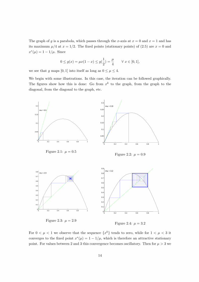
The graph of g is a parabola, which passes through the x-axis at x = 0 and x = 1 and hasits maximum µ/4 at x = 1/2. The fixed points (stationary points) of (2.5) are x = 0 andx∗(µ) = 1− 1/µ. Since

0 ≤ g(x) = µx(1− x) ≤ g(12

) =µ

4∀ x ∈ [0, 1],

we see that g maps [0, 1] into itself as long as 0 ≤ µ ≤ 4.

We begin with some illustrations. In this case, the iteration can be followed graphically.The figures show how this is done: Go from xk to the graph, from the graph to thediagonal, from the diagonal to the graph, etc.

0 0.2 0.4 0.6 0.8 10

0.05

0.1

0.15

0.2

mu = 0.5

Figure 2.1: µ = 0.5

0 0.2 0.4 0.6 0.8 10

0.05

0.1

0.15

0.2

0.25

0.3

mu = 0.9

Figure 2.2: µ = 0.9

0 0.2 0.4 0.6 0.8 10

0.1

0.2

0.3

0.4

0.5

0.6

0.7

0.8mu = 2.9

Figure 2.3: µ = 2.9

0 0.2 0.4 0.6 0.8 10

0.1

0.2

0.3

0.4

0.5

0.6

0.7

0.8

0.9

mu = 3.2

Figure 2.4: µ = 3.2

For 0 < µ < 1 we observe that the sequence xk tends to zero, while for 1 < µ < 3 itconverges to the fixed point x∗(µ) = 1 − 1/µ, which is therefore an attractive stationarypoint. For values between 2 and 3 this convergence becomes oscillatory. Then for µ > 3 we

14

0 0.2 0.4 0.6 0.8 10

0.2

0.4

0.6

0.8

1mu = 4

Figure 2.5: µ = 4.0

0 0.2 0.4 0.6 0.8 10

0.2

0.4

0.6

0.8

1

mu = 4.1

Figure 2.6: µ = 4.1

observe that the oscillations become 2-cycles. Thereafter things become more complicated,and after µ = 4 the iteration will eventually leave the interval.

In order to understand the initial convergence, we prove a simple convergence theorem forscalar iterations.

2.2.1. Let g : R1 −→ R1 be continuously differentiable and consider the iteration xk+1 =g(xk), k = 0, 1, . . .. If x∗ = g(x∗) is a stationary point, where |g′(x∗)| < 1, then thereexists a δ > 0, such that for any x0 satisfying |x0 − x∗| ≤ δ, the iteration converges to x∗.On the other hand, if |g′(x∗)| > 1, then the sequence diverges for any x0.

Proof. By the differentiability assumption we know that for any ε > 0 there exists a δ > 0such that

|g(x)− g(x∗)− g′(x∗)(x− x∗)| ≤ ε|x− x∗|, ∀ |x− x∗| ≤ δ.

If |g′(x∗)| < 1, then we can choose ε > 0, such that α = |g′(x∗)| + ε < 1. Then, for|x0 − x∗| ≤ δ, we have

|xk+1 − x∗| = |g(xk)− g(x∗)|

≤ |g′(x∗)(x− x∗)|+ |g(xk)− g(x∗)− g′(x∗)(xk − x∗)|

≤ α|xk − x∗| ≤ αk+1|x0 − x∗|

which proves the convergence. On the other hand, if |g′(x∗)| > 1, then for ε > 0 such thatα = |g′(x∗)| − ε > 1 we obtain

|xk+1 − x∗| = |g(xk)− g(x∗)|

≥ |g′(x∗)(x− x∗)| − |g(xk)− g(x∗)− g′(x∗)(xk − x∗)|

≥ α|xk − x∗| ≥ αk+1|x0 − x∗|

which implies the divergence.

15

For g(x) = µx(1 − x) we have g′(x) = µ(1 − 2x) and hence g′(0) = µ < 1 for 0 < µ < 1,and |g′(x∗(µ))| = |2 − µ| < 1 for 1 < µ < 3. In other words, for 0 < µ < 1 we havelimk→∞ x

k = 0; i.e., the population will die out. In the case µ = 1, it is readily seen,that for small positive x0 the iterates converge monotonically to zero. However, for smallnegative x0 they will diverge.

For 1 < µ < 3 it follows that limk→∞ xk = x∗(µ). More specifically, for 1 < µ < 2 the

convergence is very rapid and independent of the initial point. For 2 ≤ µ < 3 it becomesslower and, as we saw, oscillates around x∗(µ) for some time. For µ = 3 there is stillconvergence, but it is excruciatingly slow.

For µ > 3 we find that |g′(x∗(µ))| = |2−µ| > 1 and hence the sequence no longer convergesto x∗(µ) – the point has become an unstable stationary point. At the point µ = 3 the1-cycles at x∗(µ) change into two 2-cycles. Accordingly, this is called a period-doublingbifurcation point.

Our figures illustrate this. We see, how, for µ < 3 the iteration converges to a single pointand at µ = 3 switches to a 2-cycle. If one is careful, one detects the next period-doublingbifurcation point, where 4-cycles begin. This pattern continues and the period-doublingbifurcations come faster and faster and change into chaos. This can be seen in Figure 2.7.

1 2 3 40

0.5

1

mu

x

Figure 2.7: Period Doubling of the Logistic Curve

An analytical study of this quickly becomes tedious. But it is instructive to look at leastat the case of the 2-cycles:

A short calculation shows that

g2(x) = µ2x[− µx3 + 2µx2 − (1 + µ)x+ 1

]

16

and hence that the stationary points of g2 are the roots of

x− g2(x) = µ3(x− (1− 1µ

)) q2(x) = 0, q2(x) := x2 − (1 +1µ

)x+1µ

(1 +1µ

)

where we used that the stationary points of g2 include those of g. Thus the true 2-cyclesare the roots of q2; that is,

z±(µ) :=12[(1 +

1µ

)± 1µ

√(µ− 3)(µ+ 1).

These roots are only real for µ ≥ 3. Moreover for µ = 3 we have the double root z±(3) =2/3. The two roots z−(µ) and z+(µ) form a 2-cycle. In fact, because of z−(µ) + z+(µ) =1 + 1/µ a short calculation shows that

g(z−(µ)) = g(1 +1µ− z+(µ)) = z+(µ)− µq2(z+(µ)) = z+(µ)

and analogously that g(z+(µ)) = z−(µ).

From g2(x) = µg(x)(1− g(x)) it follows that (g2)′(x) = µg′(x)(1− 2g(x)). Hence, in viewof z−(µ)z+(µ) = (1/µ)(1 + 1/µ) we obtain that

(g2)′(z−(µ)) = µ2(1− 2z−(µ))(1 + 2z+(µ))

= µ2[1− 2(z−(µ) + z+(µ)) + 4z−(µ)z+(µ)]

= µ2[1− 2(1 +1µ

) + 41µ

(1 +1µ

)]

= −µ2 + 2µ+ 4

and the first line also implies that (g2)′(z−(µ)) = (g2)′(z+(µ)). For µ = 3 the quadraticpolynomial in the last line has the value 1 and for µ ≥ 3 it decreases monotonically andreaches the value −1 for µ = 1 +

√6. This implies that

|(g2)′(z−(µ))| = |(g2)′(z+(µ))| < 1 ∀3 < µ < 1 +√

6,

Thus, by the theorem the iteration with g2 converges in this µ-interval to the calculated2-cycles.

At µ = 1 +√

6 we have the next period-doubling bifurcation point, where now 4-cyclesbegin. The computation with g4 is more tedious, but shows that indeed for a small intervalbeyond 1 +

√6 the iterates converge to stable 4-cycles.

The following table shows the intervals of the 2k-cycles for the system:

17

cycle µ

2 34 3.4494908 3.54409016 3.56440732 3.56875064 3.56969128 3.56989256 3.569934512 3.5699431024 3.56994512048 3.569945557acc. pnt. 3.569945672

Obviously, the period doubling bifurcations come faster and faster and tend to the pointµ∞ ≈ 3.569945672.... It can be shown that

δ = limk→∞

µk+1 − µkµk+2 − µk+1

= 4.669201609102990...

is a constant, now known as the Feigenbaum constant. In fact, this constant is universalfor all one-dimensional maps on a bounded interval that satisfy a certain general condition.We will not go into details.

As we observed, beyond µ∞ there is chaos. We can no longer see any oscillations, andslight variations in the initial point yield dramatically different results over time.

However, there are still certain isolated values of µ, that appear to show non-chaoticbehavior; these are sometimes called islands of stability. For instance, beginning at 1 +2√

2 ≈ 3.83.. there is a range of parameters, which show a three-cycle, and, for slightlyhigher µ-values, a 6 and then a 12 cycle, etc. There are other ranges which yield 5-cycles,etc. In fact, periods of any length occur. Beyond µ = 4, the xk eventually leave theinterval [0, 1] and diverge for almost all initial values.

2.3 Periodic Behavior in Standard Iterations

The solution behavior we observed for the discrete logistic equation is by no means atyp-ical. In fact, a similar behavior arises in standard iterative methods for solving nonlinearequations.

As a very simple example suppose that we apply the standard Newton method

xk+1 = xk − f(xk)f ′(xk)

∀k = 0, 1, 2, . . . . (2.6)

18

to the cubic equationg(x) := x3 − x = 0, x ∈ R1, (2.7)

with the roots x∗1 = −1, x∗2 = 0, und x∗3 = 1. We consider the sets Aj of all startpointsx0 for which (2.6) converges to x∗j , j = 1, 2, 3. These sets are the attraction basins of theroots; they are shown in Figure 2.8.

−1 −0.5 0 0.5 1

−0.6

−0.4

−0.2

0

0.2

0.4

0.6

Figure 2.8: Attraction basins of real cubic

In particular, we see that

x0 ∈ (−∞,−1/√

3) Limit = x∗1 = −1x0 ∈ (−1/

√5, 1/√

5) Limit = x∗2 = 0x0 ∈ (1/

√3,∞) Limit = x∗3 = 1

x0 = ±(1/√

5) period 2

For x0 ∈ (−1/√

3,−1/√

5) and x0(1/√

5, 1/√

3) the behavioor is less predictable. Thereare points from where the method converges to some root and there are also points wherethe iterates cycle. In other words, the attraction domains of the three roots consists ofintervals between which there are intervals with a chaotic convergence behavior.

The situation becomes more evident for the complex cubic

z3 − z = 0, z ∈ C1. (2.8)

In terms of the real and complex parts the complex Newton method can be written as areal iterative

xk+1 = G(xk), k = 0, 1, . . . G(x) =

(x(1)3 − 3 ∗ x(1) ∗ x(2)2 − 1x(2)3 − 3 ∗ x(1)2 ∗ x(2)

), x ∈ R2.

19

−1 −0.5 0 0.5 1

−1

−0.8

−0.6

−0.4

−0.2

0

0.2

0.4

0.6

0.8

1

Figure 2.9: Attraction basins of complex cubic

Figure 2.9 shows the attraction basins of the three roots x∗r = 1, x∗± = −(1 ± i√

3)/2 indifferent colors.

We see again that each of the roots is inside an open subset of its attraction basin. Butbetween these open sets there are so called fractal sets, where the convergence is veryirregular.

A fractal is generally ”a rough or fragmented geometric shape, that can be split into parts,each of which is (at least approximately) a reduced-size copy of the whole.” This propertyis called self-similarity. The term ”fractal” was coined by Benot Mandelbrot around 1975.Because they appear to be similar at all levels of magnification, fractals are informallyconsidered to be infinitely complex. Natural objects that approximate fractals includeclouds, mountain ranges, lightning bolts, coastlines, and snow flakes. A classical exampleis the well known Sierpinski triangle shown in Figure 2.10.

The literature on fractals is large. It should be noted, that fractals arise not only indiscrete, but also in continuous dynamical systems.

2.4 The Henon Attractor

The Lorenz system showed, that simple dynamical systems (with continuous time) canshow a strange behavior. In the study of that behavior, the astronomer Michel Henon wasled to look for simpler systems, which were easier to analyze. In 1976, he introduced the

20

0

0.5

1

1.5

2

2.5

3

Figure 2.10: Sierpinski triangle

following discrete dynamical system

xk+1 = G(xk), k = 0, 1, . . . , G(x) :=

(1 + x2 − ax2

1

bx1

), x ∈ R2. (2.9)

which indeed does have a strange attractor. Here a and b are parameters, which, in theinitial configuration, were set to a = 1.4 and b = 0.3.

Generally, the determinant of the Jacobian matrix of the map denotes the expansion rateof the volume (area) per iteration in the phase space. For the Henon map, we have

DG(x) :=

(−2ax1 1b 0

)and hence |detDG(x)| = | − b| = 0.3; i.e., the map contracts areas. By taking the limit ofthe contraction rate, i.e., b = 0, we obtain the one-dimensional system xk+1 = 1− a(xk)2,which can be transformed into the logistic map.

The Henon map may be decomposed into three mappings G = G3 G2 G1, where

G1(x) :=

(x1

1 + x2 − ax21

)bends – but does not contract – an area in the x2-direction,

G2(x) :=

(bx1

x2

)is a contraction in the x1 direction, and, finally,

G3(x) :=

(x2

x1

)

21

is a reflection across the line x2 = x1.

We see this with a simple Matlab code applied to the rectangle [−1, 1]× [−1, 1] (see Figure2.11). After the second step, we observe already the emergence of a sichel-shaped figure.This is indeed an indication of what we obtain after many iterations. For this we start atan arbitrary initial point x0 in the vicinity of the sichel and iterate for several thousandsteps. If x0 is not too far away, the result will always be the same figure shown in Figure2.12. It turns out to be an attractive invariant set of G in the earlier defined sense.Although composed of lines, the orbits of points on this set do not flow continuously, butjump from one location to another.

−5 −4 −3 −2 −1 0 1 2

−1

−0.8

−0.6

−0.4

−0.2

0

0.2

0.4

0.6

0.8

1

Figure 2.11: Henon Map Steps 1,2

−1.5 −1 −0.5 0 0.5 1 1.5−0.4

−0.3

−0.2

−0.1

0

0.1

0.2

0.3

0.4

x

y

Figure 2.12: Henon Attractor

The figure is the same for all initial points, for which the iteration does not diverge, butthe resulting sequences xk are very different. In fact, even for small changes of the initialpoint, the sequences will eventually diverge from each other and evolve separately. TheHenon attractor also has a great amount of fine structure and successive magnificationsshow an ever increasing degree of detail. On closer inspection, what looks like a line turnsout to be a set of lines, and when these lines are magnified further, they also turn out tobe sets of lines, etc.

22

Chapter 3

Planar Linear Systems

In this chapter we begin with an elementary analysis of a simple class of dynamical systems,namely two-dimensional real,linear systems

x = Ax, x(0) = x0, A =

(a b

c d

). (3.1)

Planar linear systems (3.1) are not entirely artificial problems as the three simple examplesin the next section will show.

3.1 Examples of Planar Systems

3.1.1 A Shock-absorber

As a model of a shock absorber, consider a mass m supported on a vertically mountedspring, which is constrained to move only along the axis of the spring. The motion of themass is hydraulically damped. For this it is attached to a piston, that moves in a cylinderfilled with hydraulic fluid; see Figure 3.1.

c

mx

r

Figure 3.1: A Shock Absorber

23

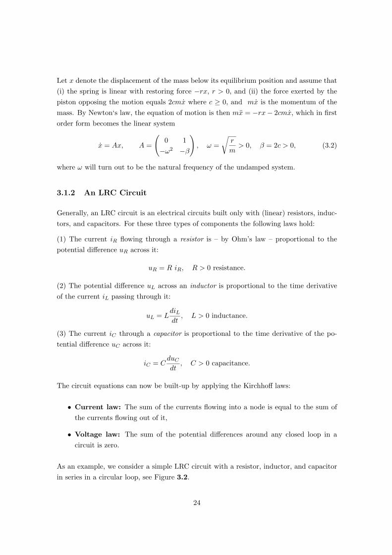
Let x denote the displacement of the mass below its equilibrium position and assume that(i) the spring is linear with restoring force −rx, r > 0, and (ii) the force exerted by thepiston opposing the motion equals 2cmx where c ≥ 0, and mx is the momentum of themass. By Newton‘s law, the equation of motion is then mx = −rx− 2cmx, which in firstorder form becomes the linear system

x = Ax, A =

(0 1−ω2 −β

), ω =

√r

m> 0, β = 2c > 0, (3.2)

where ω will turn out to be the natural frequency of the undamped system.

3.1.2 An LRC Circuit

Generally, an LRC circuit is an electrical circuits built only with (linear) resistors, induc-tors, and capacitors. For these three types of components the following laws hold:

(1) The current iR flowing through a resistor is – by Ohm’s law – proportional to thepotential difference uR across it:

uR = R iR, R > 0 resistance.

(2) The potential difference uL across an inductor is proportional to the time derivativeof the current iL passing through it:

uL = LdiLdt, L > 0 inductance.

(3) The current iC through a capacitor is proportional to the time derivative of the po-tential difference uC across it:

iC = CduCdt

, C > 0 capacitance.

The circuit equations can now be built-up by applying the Kirchhoff laws:

• Current law: The sum of the currents flowing into a node is equal to the sum ofthe currents flowing out of it,

• Voltage law: The sum of the potential differences around any closed loop in acircuit is zero.

As an example, we consider a simple LRC circuit with a resistor, inductor, and capacitorin series in a circular loop, see Figure 3.2.

24

LR

C

Figure 3.2: A simple LRC-Circuit

In this case, we obtain the equations

iR = iC = iL, current lawuR + uL + uC = 0, voltage lawuR = R iR, resistorLdiLdt = uL, inductanceC duC

dt = iC , capacitor

With u = uC and i = iR, simplification yields

du

dt=

1Ci,

di

dt= − 1

L(uR + uC) = −R

Li− 1

Lu.

This is a planar linear system (3.1) with the matrix

A =

(0 1−α −β

), α =

1LC

> 0, β = 2R

L> 0, (3.3)

which has exactly the same form as (3.2) with coefficients of the same sign.

3.1.3 An Economic Model

Consider an economy, where at time t, Y = Y (t) is the total output, C = C(t) theconsumption, I = I(t) the investment, and G the (constant) government expenditure. Ifthere are no further influences, we then require that

Y (t) = C(t) + I(t) +G. (3.4)

It is not unreasonable to assume that the consumption C(t) is proportional to the outputY (t− τ), where τ denotes a response time. If we use the first order approximation

Y (t− τ) = Y (t)− τ Y (t),

this means thatC(t) = (1− s)[Y (t)− τ Y (t)]. (3.5)

25

where s > 0 is a savings factor.

Similarly, investments may be assumed to be proportional to the change in output butagain with a time lag; i.e.,

I(t+ σ) = aY (t).

Again in first order approximation this gives

I(t) + σI(t) = aY (t). (3.6)

By substituting (3.5) into (3.4) we obtain

(1− s)τ Y (t) = −sY (t) + I(t) +G (3.7)

and hence after differentiation and substitution of (3.6)

(1− s)τ Y (t) = −sY (t) + +1σ

[aY (t)− I(t)] (3.8)

Here I(t) can be eliminated by means of (3.7). At the same time it is useful to introducethe translated variable

y = Y − G

s.

We then obtain the second order ODE

στ(1− s) y +[sσ + (1− s)τ − a

]y + s y = 0 (3.9)

In first order form this is a planar linear system (3.1) with the matrix

A =

(0 1−α −β

), α =

s

στ(1− s)> 0, β =

sσ + (1− s)τ − a2στ(1− s)

. (3.10)

Again, this matrix has an analogous form as (3.2) and (3.3), but here β need not bepositive. We will see shortly, that this has a profound effect.

3.2 Transformations of Planar Systems

For the analysis of any linear system

x = Ax

it is natural to look for a simplifying coordinate transformation x = Uy. Here U is somenonsingular matrix and the transformed system becomes

y = Qy, Q = U−1AU.

26

A principal tool for constructing transformations, which produce matrices Q of a simplerform, is the use of the eigenvalues and eigenvectors of A. We will discuss later the com-putation of eigenvalues and eigenvectors for general matrices and concentrate here on oursimple case of 2× 2 matrices

A =

(a b

c d

).

Recall, that a complex number λ is an eigenvalue of A if there exists a nonzero, complexvector u ∈ C2, such that Au = λu; that is, (A − λI)u = 0. Hence, A − λI must be asingular matrix and this holds exactly if det(A− λI) = 0.

In our case, we obtain the characteristic polynomial

pA(λ) = det(A− λI) = λ2 − tr(A)λ+ det(A) (3.11)

where tr(A) = a + d is the trace of A and det(A) = ad − bc the determinant. Obviouslythe roots of pA are

λ1,2 =12[

tr(A)±√

∆], ∆ := tr(A)2 − 4 det(A). (3.12)

Hence we have three principal cases:(a) ∆ > 0: Two distinct real eigenvalues λ1 > λ2,(b) ∆ < 0: Two conjugate complex eigenvalues λ1,2 = α± iβ,(c) ∆ = 0: A double root λ1 = λ2 = 1

2 tr(A).

There is no need for developing formulas for the corresponding eigenvectors. Instead, weconcentrate on illustrative examples for the three cases.

Case (a): We will prove later, that when the real eigenvalues λ1 and λ2, are distinct,then the corresponding eigenvectors u1, u2 are linearly independent. Clearly, Au1 = λ1u

1,Au2 = λ2u

2, is equivalent with

A(u1, u2) = (u1, u2)D, D = diag(λ1, λ2),

and for U = (u1, u2) the transformed matrix equals U−1AU = D. In the new coordinatesystem the dynamical system

y1 = λ1y1, y2 = λ1y2, y1(0) = y01, y2(0) = y0

2,

has the solutiony1(t) = exp(tλ1) y0

1, y2(t) = exp(tλ2) y02.

Case (b): For distinct conjugate complex eigenvalues λ1,2 = α± iγ and

A(v + iw) = (α+ iγ)(v + iw),

27

we haveA(v − iw) = (α− iγ)(v − iw).

Then

A(v, w) = (v, w) T, T :=

(α γ

−γ α

),

and v w are linearly independent. Hence with U = (v, w) we obtain the transformedsystem y = Ty, U−1AU = T , which has the solutions

y1(t) = c1eta cos(γt) + c2e

ta sin(γt)

y2(t) = −c1eta sin(γt) + c2eta cos(γt)

where the constants c1 c2 are chosen so as to sastify the initial conditions.

Case (c): There are two distinct subcases. If λ1,2 = a is a double eigenvalue and thereexist two linearly independent eigenvectors u1 and u2, then we have

AU = U diag(λ, λ) = λU, U = (u1, u2).

Hence U−1AU = λI2 and the tranformed system y = λy has the solution

y1(t) = exp(tλ) y01, y2(t) = exp(tλ) y0

2.

On the other hand, we will see, that there may well be only one linearly independenteigenvector u. Then it turns out, that there exists a principal vector

v ∈ R2, (A− λI2)2v = 0, (A− λI2)v 6= 0,

for which necessarily (A − λI2)v = νu. We can scale v such that ν = 1, and thereforeobtain

A(u, v) = (u, v) T, T :=

(λ 10 λ

);

which implies that u, v are linearly independent. Thus with U = (u, v) the transformedsystem equals y = Ty, T = U−1AU , and has the solutions

y1(t) = (y01 + y0

2 t) etλ, y2 = y0

2 etλ.

This, indeed, covers all likely cases and we obtained the following result:

3.2.1. Let A be a real 2 × 2 matrix with eigenvalues λ1, λ2. Then there exists a real,non-singular matrix U such that U−1AU = Q, where Q is one of the four matrices:

(a)

(λ1 00 λ2

), λ1 > λ2, (b)

(α γ

−γ α

)λ1,2 = α± iβ.

(c1)

(λ1 00 λ1

), λ1 = λ2, (c2)

(λ1 10 λ1

), λ1 = λ2,

(3.13)

28

3.3 Phase Portraits of Planar Systems

The phase portraits of the four cases in 3.2.1 are visibly different. Clearly x = 0 is the onlystationary point of the given system x = Ax. Depending on the signs of the determinantdet(A), the trace tr(A), and the discriminant ∆, we have the categorization given in thefollowing table:

Type tr det ∆ Eigenvalues

Saddles < 0 λ1 > 0 > λ2

Sources > 0 > 0 > 0 node λ1 > λ2 > 0> 0 > 0 = 0 improper node λ1 = λ2 > 0> 0 > 0 < 0 spiral (focus) λ1,2 = α± βi, α > 0

Sinks < 0 > 0 > 0 node λ1 < λ2 < 0< 0 > 0 = 0 improper node λ1 = λ2 < 0< 0 > 0 < 0 spiral (focus) λ1,2 = α± βi, α < 0

Centers = 0 > 0 < 0 λ1,2 = ±βiSingular > 0 = 0 > 0 line-source λ1 > λ2 = 0

= 0 = 0 = 0 singular-saddle λ1 = λ2 = 0< 0 = 0 > 0 line-sink λ1 < λ2 = 0

In brief, a primary classification isstable points or sinks (Senken),unstable points or sources (Quellen),saddle points (Sattel).

The stable and unstables cases have the secondary subclassesnodes (Knoten)centers (Wirbel),spiral or foci (Spirale, Brennpunkt)

Saddles have both dynamically contracting and expanding directions and we cannot speakof either stability or unstability. Figures Figure 3.3 – 3.10 show examples for the variouscases, including the last two with singular matrices.

We look also at our three examples in section 3.1. In each case the matrix had the form

A =

(0 1−α −β

). (3.14)

where, in all cases, det(A) = α > 0. In the first two examples we also had tr(A) = −β ≤ 0and hence, by our table, the origin is either a stable or asymptotically stable stationarypoint. But in the economic example we cannot exclude the case β < 0, in which case thepoint is unstable.

29

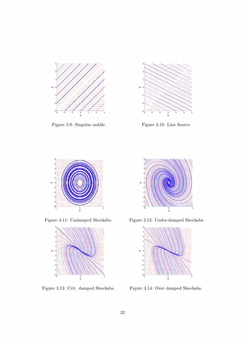
In the shock-absorber example we had

A =

(0 1−ω2 −2c

), ω =

√r

m> 0, c > 0. (3.15)

where m is the mass, r the spring constant, and c the hydraulic damping factor. Engineersdistinguish the following four cases and shown in Figures 3.11 – 3.14:(1) c = 0, undamped system with natural frequency ω. Phase portrait is a center.(2) 0 < c < ω, underdamped system. Phase portrait a spiral.(3) c = ω, critically damped system. Phase portrait an improper node.(4) c > ω, overdamped system. Phase portrait a (proper) node.

The behavior of the LRC circuit is entire analogous, except that then ω = 1√LC

> 0 andc = R

L . For the economic problem the phase portrait will again be similar to those ofthe other two example as long as in (3.14) the coefficient β is positive. Then the trace isnegative and the origin is stable. But in this case there are situation, where β < 0. Since

β =sσ + (1− s)τ − a

2στ(1− s),

there may well be negative values when the investment rate is high and the lag-times areshort. As noted, the system then becomes unstable.

30

−3 −2 −1 0 1 2 3−3

−2

−1

0

1

2

3

x

y

Figure 3.3: Source – Node

−3 −2 −1 0 1 2 3−3

−2

−1

0

1

2

3

x

yFigure 3.4: Source – Spiral

−3 −2 −1 0 1 2 3−3

−2

−1

0

1

2

3

x

y

Figure 3.5: Center

−3 −2 −1 0 1 2 3−3

−2

−1

0

1

2

3

x

y

Figure 3.6: Saddle

−3 −2 −1 0 1 2 3−3

−2

−1

0

1

2

3

x

y

Figure 3.7: Source – Improper Node 2

−3 −2 −1 0 1 2 3−3

−2

−1

0

1

2

3

x

y

Figure 3.8: Source – Improper Node 1

31

−3 −2 −1 0 1 2 3−3

−2

−1

0

1

2

3

x

y

Figure 3.9: Singular saddle

−3 −2 −1 0 1 2 3−3

−2

−1

0

1

2

3

x

y

Figure 3.10: Line Source

−5 0 5−5

−4

−3

−2

−1

0

1

2

3

4

5

x

y

Figure 3.11: Undamped Shockabs.

−5 0 5−5

−4

−3

−2

−1

0

1

2

3

4

5

x

y

Figure 3.12: Under-damped Shockabs.

−5 0 5−5

−4

−3

−2

−1

0

1

2

3

4

5

x

y

Figure 3.13: Crit. damped Shockabs.

−5 0 5−5

−4

−3

−2

−1

0

1

2

3

4

5

x

y

Figure 3.14: Over damped Shockabs.

32