Complex Networks Measures and deterministic models Philippe Giabbanelli.

Notes: Deterministic Modelsin Operations Research
J.C. ChrispellDepartment of Mathematics
Indiana University of PennsylvaniaIndiana, PA, 15705, USA
E-mail: [email protected]://www.math.iup.edu/~jchrispe
May 5, 2012

OR Notes Draft: May 5, 2012
ii
Preface
These notes will serve as an introduction to the basics of solving deterministic models inoperations research. Topics discussed will included optimization techniques and applicationsin linear programming. Specifically a discussion of sensitivity analysis, duality, and thesimplex method will be given. Additional topics to be considered include non-linear anddynamic programming, transportation models, and network models.
The majority of this course will follow the presentation given in the Operations Research:Applications and Algorithms text by Winston [8]. I will supplement the Winston text withadditional material from other popular books on operations research. For further readingyou may wish to consult:
• Introduction to Operations Research by Hillier and Lieberman [2]
• Operations Research: An Introduction by Taha [7]
• Linear Programming and its Applications by Eiselt and Sandblom [1]
• Linear and Nonlinear Programming by Luenberger and Ye [4]
• Linear and Nonlinear Programming by Nash and Sofer [5]
My Apologies in advance for any typographical errors or mistakes that are present in thisdocument. That said, I will do my very best to update and correct the document if I ammade aware of these inaccuracies.
-John Chrispell
iii

OR Notes Draft: May 5, 2012
iv
Contents
1 Introduction 1
1.1 Tabel and Chair Example . . . . . . . . . . . . . . . . . . . . . . . . . . . . 1
2 Basic Linear Algebra 7
2.0.1 The Gauss-Jordan Method for Solving Linear Systems . . . . . . . . 8
3 Linear Programming Basics 11
3.1 Parts of a Linear Program . . . . . . . . . . . . . . . . . . . . . . . . . . . . 11
3.1.1 Linear Programming Assumptions . . . . . . . . . . . . . . . . . . . . 12
3.1.2 Feasible Region and Optimal Solution . . . . . . . . . . . . . . . . . . 12
3.2 Special Cases: . . . . . . . . . . . . . . . . . . . . . . . . . . . . . . . . . . . 15
3.2.1 Example: Multiple Optimal Solutions . . . . . . . . . . . . . . . . . . 15
3.2.2 Example: Infeasible Linear Program . . . . . . . . . . . . . . . . . . 16
3.2.3 Example: Unbounded Optimal Solution . . . . . . . . . . . . . . . . 16
3.3 Setting up Linear Programs . . . . . . . . . . . . . . . . . . . . . . . . . . . 17
3.3.1 Work-Scheduling Problem: . . . . . . . . . . . . . . . . . . . . . . . . 17
4 Examples of Linear Programs 19
4.1 Diet Problem . . . . . . . . . . . . . . . . . . . . . . . . . . . . . . . . . . . 19
4.1.1 Solution Diet Problem . . . . . . . . . . . . . . . . . . . . . . . . . . 20
4.2 Scheduling Problem: . . . . . . . . . . . . . . . . . . . . . . . . . . . . . . . 21
4.2.1 Solution Scheduling Problem: . . . . . . . . . . . . . . . . . . . . . . 21
4.3 A Budgeting Problem . . . . . . . . . . . . . . . . . . . . . . . . . . . . . . . 22
4.3.1 Solution Budgeting Problem . . . . . . . . . . . . . . . . . . . . . . . 22
v

OR Notes Draft: May 5, 2012
5 The Simplex Algorithm 25
5.1 Standard Form . . . . . . . . . . . . . . . . . . . . . . . . . . . . . . . . . . 25
5.1.1 Example: . . . . . . . . . . . . . . . . . . . . . . . . . . . . . . . . . 28
5.2 Basic and Nonbasic Variables . . . . . . . . . . . . . . . . . . . . . . . . . . 28
5.2.1 Directions of Unboundedness . . . . . . . . . . . . . . . . . . . . . . 30
6 Simplex Method Using Matrix-Vector Formulas 35
6.1 Problem Using Tableaus . . . . . . . . . . . . . . . . . . . . . . . . . . . . . 35
6.2 Matrix Format of Linear Program . . . . . . . . . . . . . . . . . . . . . . . . 36
6.2.1 Initial Tableau (Matrix Form): . . . . . . . . . . . . . . . . . . . . . . 37
7 Duality 41
7.1 A Motivating Example: My Diet Problem: . . . . . . . . . . . . . . . . . . . 41
7.1.1 Cononical Form . . . . . . . . . . . . . . . . . . . . . . . . . . . . . . 43
8 Basic Duality Theory 47
8.1 Relationship Between Primal and Dual . . . . . . . . . . . . . . . . . . . . . 47
8.2 Weak Duality . . . . . . . . . . . . . . . . . . . . . . . . . . . . . . . . . . . 49
8.3 Strong Duality . . . . . . . . . . . . . . . . . . . . . . . . . . . . . . . . . . 50
8.4 The Dual Simplex Method . . . . . . . . . . . . . . . . . . . . . . . . . . . . 57
9 Sensitivity Analysis 61
9.1 Sensitivity Analysis . . . . . . . . . . . . . . . . . . . . . . . . . . . . . . . . 61
9.1.1 Verify this graphically: . . . . . . . . . . . . . . . . . . . . . . . . . . 63
9.2 Sensitivity Analysis Using Matrices . . . . . . . . . . . . . . . . . . . . . . . 64
9.2.1 Illustrating Example . . . . . . . . . . . . . . . . . . . . . . . . . . . 65
10 Non Linear Programming 71
10.1 Data Fitting . . . . . . . . . . . . . . . . . . . . . . . . . . . . . . . . . . . . 71
10.1.1 Linear Problems . . . . . . . . . . . . . . . . . . . . . . . . . . . . . 72
10.1.2 Taylor series . . . . . . . . . . . . . . . . . . . . . . . . . . . . . . . . 75
10.1.3 Newton’s Method . . . . . . . . . . . . . . . . . . . . . . . . . . . . . 75
10.2 Non-linear Least Squares . . . . . . . . . . . . . . . . . . . . . . . . . . . . . 77
vi

OR Notes Draft: May 5, 2012
11 Network Flows 79
11.1 Dijkstra’s Algorithm . . . . . . . . . . . . . . . . . . . . . . . . . . . . . . . 79
12 Appendices 83
12.1 Homework 1 . . . . . . . . . . . . . . . . . . . . . . . . . . . . . . . . . . . . 83
12.2 Homework 2 . . . . . . . . . . . . . . . . . . . . . . . . . . . . . . . . . . . . 88
12.3 Homework 3 . . . . . . . . . . . . . . . . . . . . . . . . . . . . . . . . . . . . 93
12.4 Homework 4 . . . . . . . . . . . . . . . . . . . . . . . . . . . . . . . . . . . . 101
12.5 Homework 5 . . . . . . . . . . . . . . . . . . . . . . . . . . . . . . . . . . . . 105
Bibliography 113
vii
Chapter 1
Introduction
“If you choose not to decide you still have made a choice.”
−Neil Peart
Operations Research, at its heart, uses modeling to solve applied mathematical problems inthe hopes of making optimal decisions efficiently. The term Operations Research can traceits roots back to World War II when a scientific approach was adopted to distribute resourcesbetween various military operations (scientists doing research on military operations)[2, 8].
In order to do any scientific research on a problem a mathematical model is needed. TheWInston text states:
Mathematical Model: - is a mathematical representation of an actual situation that maybe used to make a better decision or simply to understand the actual situation better. Thegoal with most models considered in this course will be to optimization some quantity (usingan objective function based on decision variables) subject to problem constraints.
Several examples where Operations Research techniques were implemented in order fordifferent organizations to obtain optimal solutions and distribution of resources (CITGOPetroleum manufacturing, The San Francisco Police Department Scheduling, GE Capitalcredit card bill repayment).
1.1 Tabel and Chair Example
Consider the following modification of an example given in [6]:
A furniture manufacturer produces two products: wooden tables and chairs. Theunit profit for the tables is $6, and the unit profit for the chairs is $8. In orderto simplify the problem assume that only resources used in the production of thetables and chairs are wood (in board feet, bf) and labor (in hours, h). It takes6 bf and 1 hour labor to make a table, and 4 bf and 2 hours labor to make a
1

OR Notes Draft: May 5, 2012
chair. There are 20 bf of wood available and 6 hours of labor available. If youwish to maximize profit what is the optimal distribution of these resources?
Formulate a Mathematical Model of the Problem
The idea now becomes to solve the given problem using a linear model or linear programming.Thus, we need to translate the real world problem into a format with mathematical equationsthat represent:
• An objective function: In this case maximize the profit.
• Decision variables: Number of Tables and Chairs to produce.
• Constraint set: We only have a limited number of resources available to use whenmanufacturing the tabels and chairs.
For this example the objective function and the constraints will all be linear functions. Weshould also impose non-negativity conditions on the resources and decision variables in thisinstance. If we do not enforce these conditions it may be possible to achieve non-physicalsolutions to the given problem.
The problem definition, and formulation are often the most difficult and import step infinding an optimal solution. Lets define the decision variables x1 and x2 as the number oftables and the number of chairs to produce respectively. It is sometimes useful to place allthe information into a table:
Resource Table x1 Chair x2 AvailableWood (bf) 6 4 20Labor (hr) 1 2 6Unit Profit $6 $8
Thus, the goal is to obtain the largest profit from the objective function by:
Maximize 6x1 + 8x2
subject to:
6x1 + 4x2 ≤ 20
x1 + 2x2 ≤ 6
x1 ≥ 0
x2 ≥ 0
the problem constraints.
2

OR Notes Draft: May 5, 2012
Solving the problem using a Graphical Approach
Lets assume that the number of chairs to be produced, x1 is on the x-axis and the numberof tables to be produced x2 is on the y−axis. First write the constraints as equalities, andthen finding the intercepts of the feasible region. Thus,
6x1 + 4x2 ≤ 20 =⇒ x2 = −3
2x1 + 5 (1.1.1)
x1 + 2x2 ≤ 6 =⇒ x2 = −1
2x1 + 3 (1.1.2)
x1 ≥ 0 x1 = 0 (1.1.3)
x2 ≥ 0 x2 = 0 (1.1.4)
(1.1.5)
Figure 1.1.1: Plot of the constraints for the table and chair example.
If all the wood is used to produce chairs (set x1 = 0 in 1.1.1):
x2 = 5 this yields point C.
If all the wood is used to produce tables (set x2 = 0 in 1.1.1):
x1 =10
3this yields point E.
If all the labor is used to produce chairs (set x1 = 0 in 1.1.2):
x2 = 3 this yields point B.
3

OR Notes Draft: May 5, 2012
If all the labor is used to produce tables (set x2 = 0 in 1.1.2):
x1 = 6 this yields point D.
Note we obtain a feasible region given by the polygon FEAB.
Plot instances of the objective function
If we now pick two values for the objective function we can determine its slope and a directionof improvement. Let z be the value of the objective function:
z = 6x1 + 8x2
Thus, if z = 0 then
6x1 + 8x2 = 0 =⇒ x2 = −3
4x1,
and if z = 8 we see
6x1 + 8x2 = 8 =⇒ x2 = −3
4x1 + 1.
The direction of improvement is d = [4, 3]T , and is illustrated in Figure 1.1.2. The optimalsolution will be obtained at the corner or edge of the feasible region that is farthest awayfrom the origin on a line parallel to the objective function contours plotted for z = 0, andz = 8. Specifically from the figure the objective function is maximized at point A when 2tables and 2 chairs are manufactured using the resources available, and yields a profit of $28.
Figure 1.1.2: Illustration of the direction of improvement.
4

OR Notes Draft: May 5, 2012
The optimal solution could have also been found by testing the objective function at eachcorner of the feasible region. Note if the same value of the objective function has beenobtained at multiple corners the optimal solution of would have been any convex combinationof the two corners. In this problem we are manufacturing discrete items (building a fractionof a table or chair doesn’t make since) so we are lucky that we obtained an integer solutionto the mathematical model.
Here we will solved this simple Linear Program graphically. In the future we will use moreadvanced algebraic techniques (such as the simplex method ) to obtain the optimal solution.For more complicated problems it will become necessary to use software packages such asLINGO. In the future we will also look to see how sensitive our optimal solution is to smallchanges.
5

OR Notes Draft: May 5, 2012
6

Chapter 2
Basic Linear Algebra
“Our weary eyes still stray to the horizon. Though down this road we’ve been so manytimes.”
−Pink Floyd
Before looking into more complicated methods of solving linear programs we need to recallsome of the basics of linear algebra.
We will use the following notation. A matrix is a rectangular array of numbers, with atypical m× n matrix A written in the form:
A =
a11 a12 . . . a1n
a21 a22 . . . a2n...
.... . .
...am1 am2 . . . amn
(2.0.1)
The element of a matrix in the ith row and jth column of matrix A will be denoted by aij.Thus, if the matrix
A =
1 1 2 35 8 13 2134 55 89 144
then a23 = 13.
We will think of a matrix with only one column as vectors (or column vectors). Similarlya matrix with only one row will be a row vector. The number of rows in a vector will defineits dimension, and the number of columns in a row vector will define its dimension.
An m-dimensional vector (row or column) where all elements are zero will be called azerovector and denoted by 0. In two dimensions
0 = [0 0] and 0 =
[00
]are zero vectors.
7

OR Notes Draft: May 5, 2012
Vectors correspond to a directed line segment from the origin in the m-dimensional plane.Thus the vectors:
u =
[12
], and w =
[−3−4
]are illustrated in Figure 2.0.1. Readers should reacquaint themselves with matrix multipli-
Figure 2.0.1: Illustration of two vectors in two-dimensional plane.
cation, matrix transposition and inner products. The use of matrices and vectors will allowfor mathematical models of linear systems to be developed and solved using linear algebra.
2.0.1 The Gauss-Jordan Method for Solving Linear Systems
The three basic types of elementary row operations (ERO) are used when solving systemsof linear equation using the Gauss-Jordan Method.
1. Multiply any row of a matrix system by a nonzero scalar.
2. Multiply any row of a matrix system by a nonzero scalar and then add that row to adifferent row of the matrix.
3. Interchange any two rows of a matrix system.
8

OR Notes Draft: May 5, 2012
Consider the following example:
x1 − 2x2 + 3x3 = 9
−x1 + 3x2 = −4
2x1 − 5x2 + 5x3 = 17
We may write this linear system in the augmented matrix system notation as
A|b =
1 −2 3 9−1 3 0 −42 −5 5 17
9

OR Notes Draft: May 5, 2012
10
Chapter 3
Linear Programming Basics
“Remember to remember meStanding still in your pastFloating fast like a hummingbird”
−Wilco
3.1 Parts of a Linear Program
We detailed earlier that the major components of a linear program:
• Decision variables.
• The objective function.
• The problem constraints.
It is also worthy to note that the coefficient of a variable in the objective function is referredto as an objective function coefficient, and less obviously the coefficients in the constraintfunctions are sometimes referred to as technological coefficients.
It will often be useful to denote the coefficients on the right-hand-side of the constraints withrhs (representing the amount of a distinct resource that is available).
We will separate non-negativity of decision variables as a separate type of constraint, andmake note that decision variables may be unrestricted in sign.
Definitions:
• A function f(x1, x2, . . . , xn) of x1, x2, . . . , xn is a linear function if and only if forsome set of constants c1, c2, . . . , cn, f(x1, x2, . . . , xn) = c1x1 + c2x2 + . . .+ cnxn.
11

OR Notes Draft: May 5, 2012
• For any linear function f(x1, x2, . . . , xn) and any number b, the inequalities f(x1, x2, . . . , xn) ≤b and f(x1, x2, . . . , xn) ≥ b are linear inequalities.
With these definitions we can define a linear programming problem or LP as an opti-mization problem for which we do the following:
• Maximize or minimize a linear function of some decision variables (our objective func-tion).
• The decision variables are subject to satisfying a set of constraints each of which is alinear inequality.
• There is also a set of sign restrictions that will be satisfied. For example decisionvariables may be non-negative or unrestricted in sign.
3.1.1 Linear Programming Assumptions
In all linear programs the objective function and constraints are effected proportionallyby the decision variables (a constant coefficient multiplies the variable in each). Linearprogramming problems also have the benefit of each decision variable being independent ofothers in its contribution to the objective function. Similarly linear constraints have thebenefit of independence. For example in the table and chair example we considered thenumber of hours of labor required to make a chair did not effect the number of hours laborrequired to manufacture a table. Thus, the left hand side of the labor constraint was theadditive sum of constants multiples of the decision variables.
In addition to the proportionality and additivity assumptions in order for LP’s to representreal situations, the divisibility assumption. That is the decision variables must be allowedto take on fractional values (we can not sell a fraction of a chair). In the future we may look atinteger programming as a way of handling problems that require a discrete valued solution.We are also going to make a certainty assumption. That is that the model parametersobjective function coefficients, the right hand side of constraints and technological coefficientsare known with certainty.
3.1.2 Feasible Region and Optimal Solution
Assuming that a point is a set of distinct values for each decision variable in an LP. Thefeasible region is the collection of all possible points that satisfy the constraints and signrestrictions on the decision variables. Points not within the feasible for a linear program areconsidered infeasible.
The optimal solution for a maximization problem then becomes the point in the LP’sfeasible region that obtains the largest value of the objective function. Similarly for a mini-mization problem the point inside the LP’s feasible region that obtains the smallest value ofthe objective function is considered the optimal solution.
12

OR Notes Draft: May 5, 2012
A second graphical example
Consider the Linear Program:
max z = x1 + x2
s.t. x1 + 5x2 ≤ 25
6x1 + 5x2 ≤ 40
x1 ≤ 5
with x1, x2 ≥ 0.
The graphical solution to the linear program is shown in Figure 3.1.1. Note the value of theobjective function is is 7.4, and that only two of the constraints are binding at the optimalsolution. We consider constraints binding if the left hand side of the constraint is equalto the right hand side when an optimal solution is achieved. The constraint x1 ≤ 5 is anexample of a nonbinding constraint.
Figure 3.1.1: Graphical solution to LP with bounded Feasible Region.
The feasible region for this LP is a convex set. A set of points is aConvex set provided aline segment between any pair of points in the set is wholly contained in the set.
13
OR Notes Draft: May 5, 2012
For any convex set S, a point P is an extreme point if each line segment that lies completelyin S and contains the point P has P as an endpoint of the line segment. Extreme pointsmay also be called corner points. We make note that:
Any LP that has an optimal solution has an extreme point that is optimal.
See the Winston text for a proof of this result. It is an important result because it narrowsour search for an optimal solution down from the whole feasible region to just the extremepoints of the set.
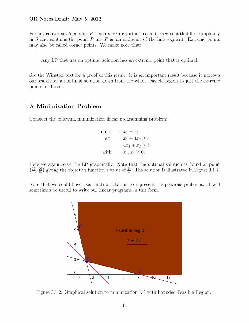
A Minimization Problem
Consider the following minimization linear programming problem:
min z = x1 + x2
s.t. x1 + 4x2 ≥ 8
4x1 + x2 ≥ 6
with x1, x2 ≥ 0.
Here we again solve the LP graphically. Note that the optimal solution is found at point(1615, 26
15
)giving the objective function a value of 14
5. The solution is illustrated in Figure 3.1.2.
Note that we could have used matrix notation to represent the previous problems. It willsometimes be useful to write our linear programs in this form.
Figure 3.1.2: Graphical solution to minimization LP with bounded Feasible Region.
14

OR Notes Draft: May 5, 2012
3.2 Special Cases:
Linear programs are not always this nice! Sometimes the linear program has an infinitenumber of solutions. Sometimes the linear program has no feasible solution, and at othertimes the solution to the linear program is unbounded.
3.2.1 Example: Multiple Optimal Solutions
Consider the following minimization linear programming problem:
max z = 3x1 + 2x2
s.t. 6x1 + 4x2 ≤ 32
−x1 + 2x2 ≤ 10
x1 ≤ 4
with x1, x2 ≥ 0.
When this LP is solved graphically as is done in Figure 3.2.3 it can be seen that there existmultiple optimal solutions. Thus, the solution to the LP becomes the convex combinationof the two extreme points represented in the graph by C and D. We can write the optimalsolution to the LP by letting α ∈ [0, 1], and stating it as a convex set:
optimal set ={
(x, y)∣∣ α (4, 2) + (1− α) (1.5, 5.75)
}. (3.2.1)
We can note that any values in the optimal set will yield a value of 16 in the objectivefunction. Use the following link to explore this problem using an interactive java applet:
http://www.math.iup.edu/~jchrispe/MATH445_545/MultipleOptimalSolutionExample.html
Figure 3.2.3: Graphical solution to maximization LP with bounded Feasible Region andmultiple optimal solutions.
15

OR Notes Draft: May 5, 2012
3.2.2 Example: Infeasible Linear Program
Consider the following minimization linear programming problem:
max z = 3x1 + 2x2
s.t. x1 + x2 ≥ 10
x2 ≤ 5.8
x1 ≤ 4
with x1, x2 ≥ 0.
Figure 3.2.4 shows the binding constraint contours and a plot of the objective functions
Figure 3.2.4: Plot of binding constraint contours and objective function contour when z = 10.
contour for a value z = 10. Note that there is no region that will satisfy all of the linearprograms constraints making this an infeasible LP.
3.2.3 Example: Unbounded Optimal Solution
Consider one last example (straight out of the Winston text). Solve again the followinglinear program graphically.
max z = 2x1 − x2
s.t. x1 − x2 ≤ 1
2x1 + x2 ≥ 6
with x1, x2 ≥ 0.
In Figure 3.2.5 it can be seen that the feasible region is unbounded in the direction ofincreasing z contours. Thus the optimal solution is unbounded.
16

OR Notes Draft: May 5, 2012
Figure 3.2.5: Plot of the feasible region for the maximization problem. Note that the feasibleregion is unbounded in the direction of increasing z contours.
3.3 Setting up Linear Programs
In many cases the difficult part of linear programming is translating a physical situationinto a mathematical model. The following are a collection of word problems that may beformulated as a linear program.
3.3.1 Work-Scheduling Problem:
This example is from the Winston text: Consider a chain of computer stores. The number ofskilled repair time the company requires during the next five months is given in the followingtable:
Month 1 (January): 6,000 hoursMonth 2 (February): 7,000 hoursMonth 3 (March): 8,000 hoursMonth 4 (April): 9,500 hoursMonth 5 (May): 11,000 hours
At the beginning of January, 50 skilled technicians work for the company. Each skilledtechnician can work up to 160 hours per month. To meet future demands, new techniciansmust be trained. It takes one month to train a new technician. During the month of trainingthe trainee must be supervised for 50 hours by an experienced technician. Each experiencedtechnician is paid $2000 a month regardless of how much he works. During the month oftraining the trainee receives $1000 for the month. At the end of each month 5% of thecompanies experienced technicians quit to find other employment. Formulate an LP for thecompany that will minimize the labor costs incurred and meet the service demands for thenext five months.
17

OR Notes Draft: May 5, 2012
18

Chapter 4
Examples of Linear Programs
“ The tall one wants white toast, dry, with nothin’ on it...And the short one wants four whole fried chickens, and a Coke.”
−Mrs. Murphy (The Blues Brothers)
In this section our goal will be to consider setting up some common types of linear programs.The list of examples given here is by no means exhaustive, and we should not for get aboutthe work scheduling problem stated in the previous section.
4.1 Diet Problem
My diet may not be nearly as poor as that of the blues brothers; however, it is probably stillpretty bad. Lets assume that my diet requires that all of my food come from my favouritefood groups: pez candy, pop tarts, Cap’N crunch, and cookies. I have the following foodsavailable for my consumption: red pez, strawberry pop-tarts, peanut butter crunch, andchocolate chip cookies. The red pez costs $0.20 per (per package), strawberry pop-tarts cost$0.50 (per package), peanut butter crunch costs $0.70 per bowl, and chocolate chip cookiescost $0.65 cents each. I must ingest at least 2500 calories a day in order to maintain mysugary lifestyle. I must also meet the following requirements I need 8 oz. of sugar, 10 oz.of fat, and 50 mg of yellow-5 food coloring. Each of my chosen foods has these requirednutrients in the following quantities:
Food Calories Sugar (oz.) Fat (oz.) yellow-5 (mg)red pez candy (per package) 50 0 .1 0.01 5strawberry pop-tarts (per package) 250 0.5 0.3 0peanut butter Cap’N crunch (per bowl) 350 1 1 4chocolate chip cookies (1 cookie) 150 0.3 0.7 1
How can I achieve my dietary constraints at a minimum cost?
19
OR Notes Draft: May 5, 2012
4.1.1 Solution Diet Problem
The first step will be do define some decision variables. Here we will define
x1 as the number of pez packages to include in my diet per dayx2 as the number strawberry pop-tart packages to consume per dayx3 as the number of bowls of peanut butter crunch to consume per dayx4 as the number of chocolate chip cookies to consume each day
Our objective function can then be defined as:
min z = 0.20x1 + 0.50x2 + 0.70x3 + 0.65x4
which will minimize the cost of our diet. The next aim is to meet the special dietary needs.Here a constraint is set up for each of the “nutrients” (calories, sugar, fat, and yellow 5).
50x1 + 250x2 + 350x3 + 150x4 ≥ 2500 (calories required)
0.1x1 + 0.5x2 + x3 + 0.3x4 ≥ 8 (sugar required)
0.01x1 + 0.3x2 + x3 + 0.7x4 ≥ 10 (fat required)
5x1 + 0x2 + 4x3 + x4 ≥ 50 (yellow-5 required)
It can also be noted that the decision variables will be non-negative in sign giving the
xi ≥ 0 for all i ∈ 1, 2, 3, 4
sign restriction.
This problem can be set up in vector notation using the above variable definitions anddefining
x =
x1
x2
x3
x4
, c =
0.200.500.700.65
, b =
2500
81050
, and
A =
50 250 350 1500.1 0.5 1 0.30.01 0.3 1 0.7
5 0 4 1
.The optimal diet can now be found by considering:
min z = cTx
s.t. Ax ≥ b
with x ≥ 0.
The optimal solution can be quickly found using the LINGO software package and the oldLINDO syntax. Open LINGO and type:
20
OR Notes Draft: May 5, 2012
min 0 .2 x 1 + 0 .5 x 2 + 0 .7 x 3 + 0.65 x 4s . t . 50 x 1 + 250 x 2 + 350 x 3 + 150 x 4 >= 25000 .1 x 1 + 0 .5 x 2 + x 3 + 0 .3 x 4 >= 80.01 x 1 + 0 .3 x 2 + x 3 + 0 .7 x 4 >= 105 x 1 + 0 x 2 + 4 x 3 + x 4 >= 50
This yields the optimal objective function value of $7.39 when
x1 = 2.016129, x2 = 0.000000, x3 = 9.979839, and x4 = 0.000000. (4.1.1)
So the minimum cost diet has me eating nothing but approximately 2 packages of pez candyand 10 bowls peanut butter crunch to meet my dietary constraints.
4.2 Scheduling Problem:
Suppose that the math department wants to schedule tutors for a cram-day before finalexams. The number of tutors needed for each four hour shift on this cram-day are:
Shift Number Time Number of Tutors Needed1 12:00 am - 4:00 am 32 4:00 am - 8:00 am 43 8:00 am - 12:00 pm 64 12:00 pm - 4:00 pm 55 4:00 pm - 8:00 pm 86 8:00 pm - 12:00 am 4
Each tutor will work two consequtive 4 hour shifts. Formulate a linear program that can beused to minimize the number of tutors needed to meet the cram-day demands.
4.2.1 Solution Scheduling Problem:
Its always best to think about the decision variable first! Here we can think about thestarting shift for the tutors.
Let xi be the number of tutors that start working on shift i.
The objective of the linear program is to minimize the number of tutors needed to meet thedemands, and we make note that summing the decision variables will count the total numberof tutors used. We should also note that since we are only concerning ourselves with 8 hourshifts for a single day, we only need to start tutors for the first five shifts. This give theobjective function:
minimizez =5∑i=1
xi
21

OR Notes Draft: May 5, 2012
Then the constraints become:
x1 ≥ 3
x1 + x2 ≥ 4
x2 + x3 ≥ 6
x3 + x4 ≥ 5
x4 + x5 ≥ 8
x5 ≥ 4
where
xi ≥ 0 for i ∈ {1, 2, . . . , 5}. (4.2.2)
Note we also added the non-negativity constraint for all the decision variables. It may havealso been nice to consider making the schedule for several cram-days in a row that again allhad the same demands for the number of tutors needed during each shift.
4.3 A Budgeting Problem
Two investments with varying cash flows (in thousands of dollars) are available.
Investment Cash Flow Year 0 Cash Flow Year 1 Cash Flow Year 2 Cash Flow Year 31 -6 - 5 7 92 -8 -3 9 7
Assuming at time 0 that $10,000 is available to invest, and after one year there will be $7,000available to invest. We will also assume an annual interest rate of 10% is available. We shallalso assume that any fraction of an investment may be purchased. Lets find a linear programthat will determine the maximum net present value obtained from the two investments.
4.3.1 Solution Budgeting Problem
We set up the linear program as follows. First the decision variables:
Let xi be the amount of investment i to purchase (i = 1, 2).
Our goal is to maximize the net present value of the investments purchased so we shouldfind the net present value of each investment for use in our objective functions.
Net present value: We need to discount each of the cash flows back to the present usinga discount factor based on the interest rate. Note that
$1.00 Today −→ $1.00 + 0.10($1.00) = $1.00(1.10) One Year From Now
22

OR Notes Draft: May 5, 2012
Thus,
$1.00 one year from now −→(
1
1.10
)$1.00 ≈ $0.9090909 today.
We can use (1
1 + r
)nas a discount factor for rate r in year n.
Let NPV1 denote the net present value of investment 1.
NPV1 = −6000 + (−5000)
(1
1.1
)1
+ 7000
(1
1.1
)2
+ 9000
(1
1.1
)3
≈ 2001.503
Let NPV2 denote the net present value of investment 2.
NPV2 = −8000 + (−3000)
(1
1.1
)1
+ 9000
(1
1.1
)2
+ 7000
(1
1.1
)3
≈ 1969.947
The objective function for the linear program is then:
maximize z = 2001.50x1 + 1969.94x2.
The constraints on the linear program are based on the amount of cash we have on hand foreach of the first two years, and the additional constraint that we may only purchase upto100% of each of the two investments. This gives
6000x1 + 8000x2 ≤ 10000
5000x1 + 3000x2 ≤ 7000
x1 ≤ 1
x2 ≤ 1
as our constraints, and we have the sign restriction that x1 and x2 are non-negative:
x1 ≥ 0, and x2 ≥ 0.
Note we can solve this linear program graphically and Figure 4.3.1 illustrates the feasiblesolution to the problem. We can see by looking for the optimal objective function contourthat the optimal investment involves 100% of investment 1 and 50% of investment 2 givingthe optimal net present value of the cash flow as:
z = 2001.50(1) + 1969.94(0.5) = 2986.47
Note that there are an infinite number of different problems that may be formulated as linearprograms. It is strongly recommended that the interested reader look over more examplespresented in [8] and other texts.
23

OR Notes Draft: May 5, 2012
Figure 4.3.1: Feasible region for the budgeting problem with an illustration of a z contour.
24

Chapter 5
The Simplex Algorithm
“Don’t wanna wait ’til tomorrowWhy put it off another day?One by one, little problemsBuild up and stand in our way, oh”
−Van Halen
The linear programs that we have been able to solve with out the assistance of a softwarepackage so far have all been in two variables. In general linear programs have many variablesand the goals of this chapter will be:
• Transform a linear programming problem into a standard form.
• Look at basic and nonbasic variables.
• Introduce the Simplex Algorithm for solving linear programming problems.
5.1 Standard Form
As we have seen there are several different ways of writing the objective function for a linearprogram (maximize profit, minimize cost). Additionally the constraints come in all differentforms too (≤,≥,=) so when discussing a systematic method for solving linear programs itwill be advantages to having written or converted the linear program to a standard form.We will consider the following linear programs to be in standard form:
minimize z = cTx, maximize z = −cTx,subject to Ax = b, subject to Ax = b,
x ≥ 0. x ≥ 0.
where b, c, and x represent vectors of length n, and A is an m × n constraint matrix, andb ≥ 0.
25

OR Notes Draft: May 5, 2012
Notice that:
• The decision variables are constrained to be non-negative.
• All of the constraints are set up to be equalities.
• The components of the right hand side vector b are non-negative.
The observation that a maximization problem could be converted to a minimization problemby multiplying every coefficient in the objective function by a ‘-1’ can be made. After theproblem is solved the objective value would then need to be multiplied by ‘-1’ again in orderto obtain the solution to the desired problem. The decision variable values obtained wouldbe the same for both objective functions. Lets consider transforming the following linearprogram into a standard form minimization problem:
maximize z = 3x1 +4x2 −7x3
subject to 7x1 +x2 +4x3 ≤ 26−2x1 +4x2 +6x3 ≤ −2
6x1 +3x2 −4x3 ≥ 4x3 ≥ 5
with x1 ≥ 0 and x2 free.
Objective function: The problem could be written using the equivalent objective function:
minimize z = −3x1 − 4x2 + 7x3
where z = −z once the optimal solution has been found.
Non-negative right had side: In order to continue converting the given LP to standardform we next consider the constraints. We would like to have all the right hand side coef-ficients be non-negative. Thus, the third constraint in the given linear program should bemultiplied by a ‘-1’ yielding:
−2x1 + 4x2 + 6x3 ≤ −2 −→ 2x1 − 4x2 − 6x3 ≤ 2
Non-zero lower bounds: In the original statement of the problem we note that the 4thconstraint has:
x3 ≥ 5.
To convert this to a standard form constraint we make a change of variables and define:
x3 = x3 − 5
This allows us to replace x3 with x3 throughout and changes the constraint
x3 ≥ 5 −→ x3 + 5 ≥ 5 −→ x3 ≥ 0.
26

OR Notes Draft: May 5, 2012
Note we need to modify the other constraints and objective function as well. For our exampleproblem we may redefine
z = −z − 35 −→ z = −z − 35
for the modified objective function. For the moment we will leave upper bounds on variablesright in the coefficient matrix.
Free variables: In the given problem we make note that x2 is a free variable. Free variablesmay be converted to non-negative constraints by defining
x2 = x′2 − x′′2 with x′2, x′′2 ≥ 0.
and we will have x′2 to handle the positive values of x2 and the new variable x′′2 will takecare of the negative pieces. There are other ways to handel free variables, and one is to usea free variable as a way of eliminating a constraint (think about this for a future homeworkassignment).
After applying all of the discussed techniques to our linear programming problem we are leftwith the following LP:
minimize z = −3x1 −4x′2 + 4x′′2 +7x3
subject to 7x1 +x′2 − x′′2 +4x3 ≤ 62x1 −4x′2 + 4x′′2 −6x3 ≥ 326x1 +3x′2 − 3x′′2 −4x3 ≥ 24
with x1, x′2, x′′2, x3 ≥ 0.
Equality constraints: In order for the constraints we consider adding slack and excessvariables to enforce the equality constraint. For the constraint:
7x1 + x′2 − x′′2 + 4x3 ≤ 6
let s1 be a slack variable such that s1 ≥ 0 and
7x1 + x′2 − x′′2 + 4x3 + s1 = 6.
For the other two constraints we use excess variables e1 ande2. Thus,
2x1 − 4x′2 + 4x′′2 − 6x3 ≥ 32 =⇒ 2x1 − 4x′2 + 4x′′2 − 6x3 − e1 = 32
and6x1 + 3x′2 − 3x′′2 − 4x3 ≥ 24 =⇒ 6x1 + 3x′2 − 3x′′2 − 4x3 − e2 = 24
with e1, e2 ≥ 0. We can now restate the full linear program in standard form:
minimize z = −3x1 −4x′2 + 4x′′2 +7x3
subject to 7x1 +x′2 − x′′2 +4x3 +s1 = 62x1 −4x′2 + 4x′′2 −6x3 −e1 = 326x1 +3x′2 − 3x′′2 −4x3 −e2 = 24
with x1, x′2, x′′2, x3, s1, e1, e2 ≥ 0.
27

OR Notes Draft: May 5, 2012
5.1.1 Example:
Try writing the following linear programs in standard form:
maximize z = 3x1 +5x2 −4x3
subject to 7x1 −2x2 −3x3 ≥ 4−2x1 +4x2 +8x3 = −3
5x1 −3x2 −2x3 ≤ 9
with x1 ≥ 1, x2 ≤ 7, and x3 ≥ 0.
After manipulation we obtain:
maximize z = 3x1 +5x′2 − 5x′′2 −4x3
subject to −7x1 +2x′2 − 2x′′2 +3x3 ≤ 32x1 −4x′2 + 4x′′2 −8x3 = 15x1 −3x′2 + 3x′′2 −2x3 ≤ 4
x′2 − x′′2 ≤ 7
with x1, x′2, x′′2, x3 ≥ 0 and z = z + 3.
We need to take this one more step and include slack variables. Thus,
maximize z = 3x1 +5x′2 − 5x′′2 −4x3
subject to −7x1 +2x′2 − 2x′′2 +3x3 +s1 = 32x1 −4x′2 + 4x′′2 −8x3 = 15x1 −3x′2 + 3x′′2 −2x3 +s2 = 4
x′2 − x′′2 +s3 = 7
with x1, x′2, x′′2, x3, s1, s2, s3 ≥ 0 and z = z + 3.
5.2 Basic and Nonbasic Variables
Lets assume that we have a standard form linear program.
minimize z = cTx,subject to Ax = b,
x ≥ 0.(5.2.1)
where b, c, and x represent vectors of length n, and A is an m× n constraint matrix (withn ≥ m), and b ≥ 0. The constraints to the linear program are given by:
Ax = b.
28

OR Notes Draft: May 5, 2012
Definition 5.2.1 A basic solution to Ax = b is obtained by setting n−m variables equalto 0 and solving for the values of the remaining m variables. This assumes that the columnsremaining m variables are linearly independent.
To find a basic solution to Ax = b, we simply choose a set of n−m variables (and set theseto zero) to be the nonbasic variables or NBV. The remaining variables will be our basicvariables or BV that are used to satisfy the constraints.
Consider the following example:
x1 + x2 = 6
−x2 + x3 = 4
Here we get to pick one nonbasic variable as we have two equations and three unknowns.Thus,
NBV = {x3}, then BV = {x1, x2}.The values of the basic variables x1, and x2 are found by solving the two equations with x3
set to zero. Thus,x2 = −4 and x1 = 10
If we choose x1 to be the nonbasic variable then the basic variables
x2 = 6 and x3 = 10.
We should note that not all sets of basic variables will yield a feasible solution to a set ofconstraints.
Consider the constraints
x1 + 2x2 + 4x3 = 4
x1 + 4x2 + 8x3 = 6.
If x1 is taken to be the nonbasic variable then the system becomes:
2x2 + 4x3 = 4
4x2 + 8x3 = 6
a system with no feasible solution and yielding no basic solution to BV = {x2, x3}.
Definition 5.2.2 Any basic solution to (5.2.1) in which all variables are nonnegative is abasic feasible solution.
When solving linear programs we are interested in sets of variables that will satisfy all of theconstraints given by Ax = b as well as also satisfying the nonnegativity constraint for thelinear program stated in standard form. We also know that
29

OR Notes Draft: May 5, 2012
Any LP that has an optimal solution has an extreme point that is optimal.
So a good place to start looking for these optimal extreme points is at basic feasible solutions.It can be shown that:
Theorem 5.2.1 A point in the feasible region of a linear program is an extreme point if andonly if it is a basic feasible solution to the LP.
A proof can be found in [3].
Example: The goal of this example is to show the relationship between extreme points andbasic feasible solutions. Given
maximize z = 4x1 + 3x2
subject to x1 + x2 ≤ 42x1 + x2 ≤ 6
with x1, x2 ≥ 0,
write the LP in standard form by adding two slack variables s1 and s2. Standard form:
maximize z = 4x1 + 3x2
subject to x1 + x2 + s1 = 42x1 + x2 + s2 = 6
with x1, x2, s1, s2 ≥ 0.
The feasible region for the linear program is shown if Figure 5.2.1. Note that all of the cornerextreme points correspond to a basic feasible solution to the linear program. We note thatthe intersection at points E, and F are not basic feasible solutions because not all of thebasic variables satisfy the nonnegativity constraint for the linear program in standard form.
5.2.1 Directions of Unboundedness
Assume that we have a standard form linear program.
minimize z = cTx,subject to Ax = b,
x ≥ 0.
where b, c, and x represent vectors of length n, and A is an m× n constraint matrix (withn ≥ m), and b ≥ 0. The feasible solutions for this linear program will be denoted by S.
30

OR Notes Draft: May 5, 2012
Figure 5.2.1:
Definition 5.2.3 An n by 1 vector d is a direction of unboundedness if for all x in S,and c ≥ 0 then
x + cd ∈ S.
This means we can move as far as we desire in the direction of d and still have a feasiblesolution to the linear program.
Consider the following example
minimize z x1 + x2,subject to 7x1 + 2x2 ≥ 28
2x1 + 12x2 ≥ 24x1, x2 ≥ 0.
Written in standard form by adding excess variables we obtain,
minimize z x1 + x2,subject to 7x1 + 2x2 − e1 = 28
2x1 + 12x2 − e2 = 24x1, x2, e1, e2 ≥ 0.
What are the basic feasible solutions for the LP.
31
OR Notes Draft: May 5, 2012
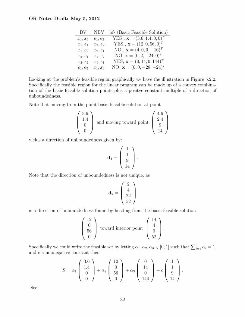
BV NBV bfs (Basic Feasible Solution)x1, x2 e1, e2 YES , x = (3.6, 1.4, 0, 0)T
x1, e1 x2, e2 YES , x = (12, 0, 56, 0)T
x1, e2 x2, e1 NO , x = (4, 0, 0,−16)T
x2, e1 x1, e2 NO, x = (0, 2,−24, 0)T
x2, e2 x1, e1 YES, x = (0, 14, 0, 144)T
e1, e2 x1, x2 NO, x = (0, 0,−28,−24)T
Looking at the problem’s feasible region graphically we have the illustration in Figure 5.2.2.Specifically the feasible region for the linear program can be made up of a convex combina-tion of the basic feasible solution points plus a positve constant multiple of a direction ofunboundedness.
Note that moving from the point basic feasible solution at point3.61.400
and moving toward point
4.62.4914
yields a direction of unboundedness given by:
d1 =
11914
.
Note that the direction of unboundedness is not unique, as
d2 =
242252
is a direction of unboundedness found by heading from the basic feasible solution
120560
toward interior point
144052
.
Specifically we could write the feasible set by letting α1, α2, α3 ∈ [0, 1] such that∑3
i=1 αi = 1,and c a nonnegative constant then
S = α1
3.61.400
+ α2
120560
+ α3
0140
144
+ c
11914
.
See
32

OR Notes Draft: May 5, 2012
Figure 5.2.2: The feasible region is shown. Note that the region may be made up of a convexcombination of basic feasible solutions plus a direction of unboundedness.
http://www.math.iup.edu/~jchrispe/MATH445_545/DirectionOfUnboundedness.html
for an interactive version of the solution.
33

OR Notes Draft: May 5, 2012
34
Chapter 6
Simplex Method Using Matrix-VectorFormulas
“Learn to be positive, it’s your only chance.”
−The Kinks
Lets consider looking at the simplex algorithm using Matrices and compare that with thetableau format we have been using.
6.1 Problem Using Tableaus
Consider the following linear program:
maximize z = 3x1 + 5x2
subject to x1 ≤ 42x2 ≤ 12
3x1 + 2x2 ≤ 18x1, x2 ≥ 0.
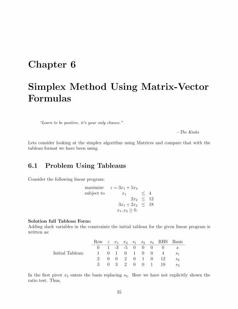
Solution full Tableau Form:Adding slack variables in the constraints the initial tableau for the given linear program iswritten as:
Initial Tableau:
Row z x1 x2 s1 s2 s3 RHS Basis0 1 -3 -5 0 0 0 0 z1 0 1 0 1 0 0 4 s1
2 0 0 2 0 1 0 12 s2
3 0 3 2 0 0 1 18 s3
In the first pivot x2 enters the basis replacing s2. Here we have not explicitly shown theratio test. Thus,
35

OR Notes Draft: May 5, 2012
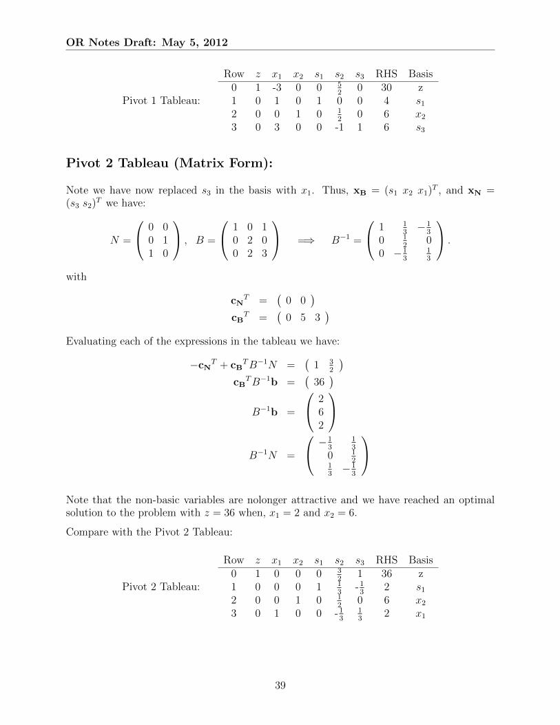
Pivot 1 Tableau:
Row z x1 x2 s1 s2 s3 RHS Basis0 1 -3 0 0 5
20 30 z
1 0 1 0 1 0 0 4 s1
2 0 0 1 0 12
0 6 x2
3 0 3 0 0 -1 1 6 s3
The next iteration of the simplex method shows that it is desirable to have x1 enter the basisand replace s3. (Note again we are not showing the ratio text.) Doing this pivot yields:
Pivot 2 Tableau:
Row z x1 x2 s1 s2 s3 RHS Basis0 1 0 0 0 3
21 36 z
1 0 0 0 1 13
-13
2 s1
2 0 0 1 0 12
0 6 x2
3 0 1 0 0 -13
13
2 x1
Here we have obtained an optimal tableau. We can see here that z is maximized at $36,000when x1 = 2 and x2 = 6.
6.2 Matrix Format of Linear Program
A standard form linear program in matrix form is written as:
maximize z = cTxsubject to Ax = b
x ≥ 0.
Thus, for the example problem we make the following definitions:
x =
x1
x2
s1
s2
s3
, c =
35000
, b =
41218
and
A =
1 0 1 0 00 2 0 1 03 2 0 0 1
.
In order to implement the simplex algorithm in matrix format we break the given coefficientmatrix A into to parts: a basic part and a non-basic part. Thus,
A = [N |B]
and similarly we separate the vectors x, and c into their basic and non-basic parts:
x =
(xNxB
), where xN =
(x1
x2
)and xB =
s1
s2
s3
36

OR Notes Draft: May 5, 2012
c =
(cNcB
), where cN =
(35
)and cB =
000
.
We can now make note of the correspondence between the simplex method as we know it intableau format, and the defined matrices. Any current basis may be written as:
xNT xB
T RHS Basis−cN
T + cBTB−1N 0 cB
TB−1b zB−1N I B−1b xB
6.2.1 Initial Tableau (Matrix Form):
For the starting basis xB = (s1 s2 s3)T , and xN = (x1 x2)T we have:
N =
1 00 23 2
, B =
1 0 00 1 00 0 1
=⇒ B−1 =
1 0 00 1 00 0 1
.
with
cNT =
(3 5
)cB
T =(
0 0 0)
Evaluating each of the expressions in the tableau we have:
−cNT + cB
TB−1N =(−3 −5
)cB
TB−1b =(
0)
B−1b =
41218
B−1N =
1 00 23 2
Ratio Test:
Note that both non-basic variables are attractive, and we choose x2 to enter the basis. Doingthe ratio test using the second column of B−1N and the current right hand side vector B−1b:
min
{12
2= 6,
18
2= 9
}and we choose s2 to leave the basis. Note we have ignored the comparison of 4 over 0 in theratio test.
Compare the above values with the tableau:
37

OR Notes Draft: May 5, 2012
Initial Tableau:
Row z x1 x2 s1 s2 s3 RHS Basis0 1 -3 -5 0 0 0 0 z1 0 1 0 1 0 0 4 s1
2 0 0 2 0 1 0 12 s2
3 0 3 2 0 0 1 18 s3
Pivot 1 Tableau (Matrix Form):
Note we have now replaced s2 in the basis with x2. Thus, xB = (s1 x2 s3)T , and xN =(x1 s2)T we have:
N =
1 00 13 0
, B =
1 0 00 2 00 2 1
=⇒ B−1 =
1 0 00 1
20
0 −1 1
.
with
cNT =
(3 0
)cB
T =(
0 5 0)
Evaluating each of the expressions in the tableau we have:
−cNT + cB
TB−1N =(−3 5
2
)cB
TB−1b =(
30)
B−1b =
466
B−1N =
1 00 1
2
3 −1
Ratio Test:
Note that the non-basic variable x1 should be picked to enter the basis. Doing the ratio testusing the first column of B−1N and the current right hand side vector B−1b:
min
{4
1= 4,
6
3= 2
}and we choose s3 to leave the basis. Note we have ignored the comparison of 6 over 0 wherex2 would potentially leave the basis in the ratio test.
Compare values with the Piviot 1 Tableau:
38
OR Notes Draft: May 5, 2012
Pivot 1 Tableau:
Row z x1 x2 s1 s2 s3 RHS Basis0 1 -3 0 0 5
20 30 z
1 0 1 0 1 0 0 4 s1
2 0 0 1 0 12
0 6 x2
3 0 3 0 0 -1 1 6 s3
Pivot 2 Tableau (Matrix Form):
Note we have now replaced s3 in the basis with x1. Thus, xB = (s1 x2 x1)T , and xN =(s3 s2)T we have:
N =
0 00 11 0
, B =
1 0 10 2 00 2 3
=⇒ B−1 =
1 13−1
3
0 12
00 −1
313
.
with
cNT =
(0 0
)cB
T =(
0 5 3)
Evaluating each of the expressions in the tableau we have:
−cNT + cB
TB−1N =(
1 32
)cB
TB−1b =(
36)
B−1b =
262
B−1N =
−13
13
0 12
13−1
3
Note that the non-basic variables are nolonger attractive and we have reached an optimalsolution to the problem with z = 36 when, x1 = 2 and x2 = 6.
Compare with the Pivot 2 Tableau:
Pivot 2 Tableau:
Row z x1 x2 s1 s2 s3 RHS Basis0 1 0 0 0 3
21 36 z
1 0 0 0 1 13
-13
2 s1
2 0 0 1 0 12
0 6 x2
3 0 1 0 0 -13
13
2 x1
39

OR Notes Draft: May 5, 2012
40

Chapter 7
Duality
“I’d like to change your mind by hitting it with a rock.”
−They Might Be Giants
As is often the case you may look at problems form many different perspectives. Thisis the case with linear programs. Lets consider a problem form our past in two differentperspectives.
7.1 A Motivating Example: My Diet Problem:
Recall from earlier this semester that I have a really bad diet that requires that all of myfood come from my favourite food groups: pez candy, pop tarts, Cap’N crunch, and cookies.I have the following foods available for my consumption: red pez, strawberry pop-tarts,peanut butter crunch, and chocolate chip cookies. The red pez costs $0.20 per (per package),strawberry pop-tarts cost $0.50 (per package), peanut butter crunch costs $0.70 per bowl,and chocolate chip cookies cost $0.65 cents each. I must ingest at least 2500 calories a dayin order to maintain my sugary lifestyle. I must also meet the following requirements I need8 oz. of sugar, 10 oz. of fat, and 50 mg of yellow-5 food coloring. Each of my chosen foodshas these required nutrients in the following quantities:
Food Calories Sugar (oz.) Fat (oz.) yellow-5 (mg) Price ($)pez candy (per package) 50 0 .1 0.01 5 0.20pop-tarts (per package) 250 0.5 0.3 0 0.50Cap’N crunch (per bowl) 350 1 1 4 0.70cookies (1 cookie) 150 0.3 0.7 1 0.65
How can I achieve my dietary constraints at a minimum cost?
Primal Solution To Diet Problem:
The first step will be do define some decision variables. Here we will define
41

OR Notes Draft: May 5, 2012
x1 as the number of pez packages to include in my diet per dayx2 as the number strawberry pop-tart packages to consume per dayx3 as the number of bowls of peanut butter crunch to consume per dayx4 as the number of chocolate chip cookies to consume each day
Our objective function can then be defined as:
min z = 0.20x1 + 0.50x2 + 0.70x3 + 0.65x4
which will minimize the cost of our diet. The next aim is to meet the special dietary needs.Here a constraint is set up for each of the “nutrients” (calories, sugar, fat, and yellow 5).
50x1 + 250x2 + 350x3 + 150x4 ≥ 2500 (calories required)
0.1x1 + 0.5x2 + x3 + 0.3x4 ≥ 8 (sugar required)
0.01x1 + 0.3x2 + x3 + 0.7x4 ≥ 10 (fat required)
5x1 + 0x2 + 4x3 + x4 ≥ 50 (yellow-5 required)
It can also be noted that the decision variables will be non-negative in sign giving the
xi ≥ 0 for all i ∈ {1, 2, 3, 4}
sign restriction.
This problem can be set up in vector notation using the above variable definitions anddefining
x =
x1
x2
x3
x4
, c =
0.200.500.700.65
, b =
2500
81050
, and
A =
50 250 350 1500.1 0.5 1 0.30.01 0.3 1 0.7
5 0 4 1
.The optimal diet can now be found by considering:
min z = cTx
s.t. Ax ≥ b
with x ≥ 0.
Dual of Diet Problem
A second way to consider the problem. Suppose that I know a nutrient salesman (WillyLoman) who will sell me supplements that taste just as good as the items in my diet.Specifically Mr. Loman sells calories, sugar, Fat, and yellow-5 and wants to sell me theseitems in order to meet my daily needs at the maximum price I’m willing to pay. Thendefining the decision variables:
42

OR Notes Draft: May 5, 2012
y1 is the price to charge me per calorie.
y2 is the price to charge me per ounce of sugar.
y3 is the price to charge me per ounce of fat.
y4 is the price to charge me per mg of yellow-5.
Loman’s objective function for my diet would look like:
max w = 2500y1 + 8y2 + 10y3 + 50y4
The constraints for the salesman are found using the available foods. Mr. Loman being agreat salesman needs to set his prices low enough that I will purchase his nutrients ratherthan my regular diet of pez and cookies. Thus, he is subject to the constraints:
50y1 + 0.1y2 + 0.01y3 + 5y4 ≤ 0.20 ( the price of pez)
250y1 + 0.5y2 + 0.3y3 + 0y4 ≤ 0.50 ( the price of pop-tarts)
350y1 + y2 + y3 + 4y4 ≤ 0.70 ( the price of Cap’N crunch)
150y1 + 0.3y2 + 0.7yy + y4 ≤ 0.65 ( the price of cookies)
where the sign restriction on the decision variables is:
yi ≥ 0 for all i ∈ {1, 2, 3, 4}Writing this in matrix form in terms of the values defined for the primal problem we have:
max w = bTy
s.t. ATy ≤ c
with y ≥ 0
wherey = (y1 y2 y3 y4)T .
These two linear programs have the same optimal solution values.
7.1.1 Cononical Form
The cononical form of a primal and its corresponding dual linear program are given as follows:
min z = cTx
s.t. Ax ≥ b
with x ≥ 0.
max w = bTy
s.t. ATy ≤ c
with y ≥ 0
Primal Dual
43

OR Notes Draft: May 5, 2012
Taking Dual of General Linear Programs
What if we don’t start in canonical form? Lets consider the constraints first:
min z = cTx
s.t. A1x ≥ b1
A2x ≤ b2
A3x = b3
with x ≥ 0.
Transform the above problem into standard canonical form (ignoring that the RHS may benegative for a moment).
min z = cTx
s.t. A1x ≥ b1
−A2x ≥ −b2
A3x ≥ b3
−A3x ≥ −b3
with x ≥ 0.
Taking the dual we have:
max w = bT1 y1 − bT2 y′2 + bT3 y′3 − bT3 y′′3s.t. AT1 y1 − AT2 y′2 + AT3 y′3 − AT3 y′′3 ≤ c
with y1,y′2,y
′3,y
′′3 ≥ 0.
Making the change of variables:
y2 = −y′2 and y3 = y′3 − y′′3
and we have:
max w = bT1 y1 + bT2 y2 + bT3 y3
s.t. AT1 y1 + AT2 y2 + AT3 y3 ≤ c
with y1 ≥ 0,y2 ≤ 0,y3 is free
What if the variables are not in standard form?
min z = cT1 x1 + cT2 x2 + cT3 x3
s.t. A1x1 + A2x2 + A3x3 ≥ b
with x1 ≥ 0,x2 ≤ 0,x3 is free
Here we make a change of variables and place the problem back into a canonical form. Let
x2 = −x′2 and x3 = x3′ − x′′3
44

OR Notes Draft: May 5, 2012
with
x′2,x′3, and x′′3 ≥ 0.
Then
min z = cT1 x1 − cT2 x′2 + cT3 x′3 − cT3 x′′3s.t. A1x1 − A2x
′2 + A3x
′3 − A3x
′′3 ≥ b
with x1,x′2,x
′3,x
′′3 ≥ 0
We can now take the Dual:
max z = bTy
s.t. AT1 y ≤ c1
−AT2 y ≤ −c2
AT3 y ≤ c3
−AT3 y ≤ −c3
with y ≥ 0
Adjusting the RHS to be non-negative:
max z = bTy
s.t. AT1 y ≤ c1
AT2 y ≥ c2
AT3 y = c3
with y ≥ 0
Relationship Between Primal and Dual
The following table summarizes the relationship between the primal and the dual problem.
Primal / Dual Constraint Dual/Primal Variableconsistent with canonical form ⇐⇒ variable ≥ 0reversed from canonical form ⇐⇒ variable ≤ 0
equality constraint ⇐⇒ variable is free
Examples:
As an exercise find the dual of the following linear programs:
45

OR Notes Draft: May 5, 2012
• Problem 1:
max z = x1 + x2
s.t. x1 − x2 ≤ 1
with x1, x2 ≥ 0
We need a dual variable y for each constraint. Thus,
min w = y1
s.t. y1 ≥ 1
−y1 ≥ 1
with y2 ≥ 0.
• Problem 2:
min z = 4x1 − 9x2 + 10x3
s.t. 5x1 + 6x2 + 7x3 ≥ 3
3x1 + 2x2 + 1x3 ≤ 4
−1x1 + 8x2 + 2x3 ≤ 5
with x1 ≥ 0, x2 ≤ 0, x3 is free
And the dual of the linear program is:
max z = 3y1 + 4y2 + 5y3
s.t. 5y1 + 3y2 − y3 ≤ 4
6y1 + 2y2 + 8y3 ≥ −9
7y1 + y2 + 2y3 = 10
with y1 ≥ 0, y2 ≤ 0, y3 ≤ 0
46
Chapter 8
Basic Duality Theory
“Read dozens of books about heroes and crooks, and I learned much from both of theirstyles.”
− Jimmy Buffet
Here we will consider the major results that relate the primal and the dual linear program-ming problems.
8.1 Relationship Between Primal and Dual
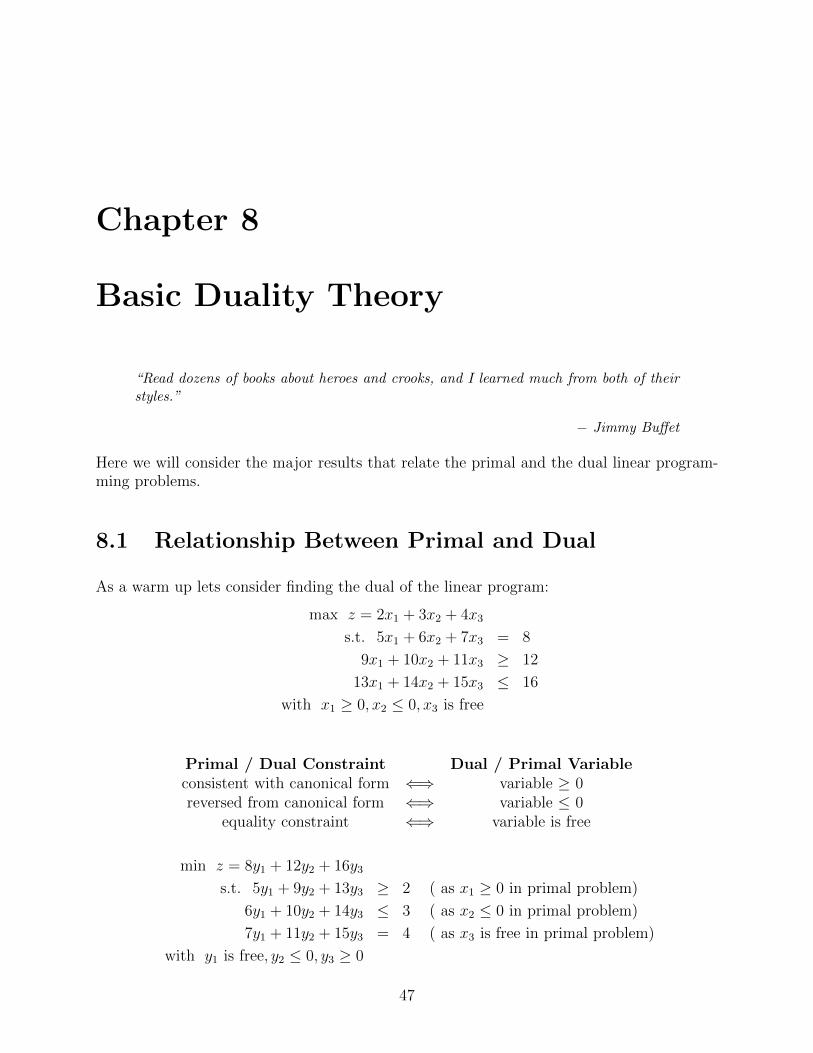
As a warm up lets consider finding the dual of the linear program:
max z = 2x1 + 3x2 + 4x3
s.t. 5x1 + 6x2 + 7x3 = 8
9x1 + 10x2 + 11x3 ≥ 12
13x1 + 14x2 + 15x3 ≤ 16
with x1 ≥ 0, x2 ≤ 0, x3 is free
Primal / Dual Constraint Dual / Primal Variableconsistent with canonical form ⇐⇒ variable ≥ 0reversed from canonical form ⇐⇒ variable ≤ 0
equality constraint ⇐⇒ variable is free
min z = 8y1 + 12y2 + 16y3
s.t. 5y1 + 9y2 + 13y3 ≥ 2 ( as x1 ≥ 0 in primal problem)
6y1 + 10y2 + 14y3 ≤ 3 ( as x2 ≤ 0 in primal problem)
7y1 + 11y2 + 15y3 = 4 ( as x3 is free in primal problem)
with y1 is free, y2 ≤ 0, y3 ≥ 0
47

OR Notes Draft: May 5, 2012
What is the dual of a problem that is written in our typical standard form?
min z = cTx
s.t. Ax = b
with x ≥ 0
Here we write the dual as:
max w = bTy
s.t. ATy ≤ c ( as x ≥ 0 in primal problem).
with y is free
Graph the following Example:
max z = 2x1 + x2
s.t. x1 ≤ 1
x2 ≤ 1
with x1 and x2 ≥ 0
Taking the dual:
min w = y1 + y2
s.t. y1 ≥ 2
y2 ≥ 1
with y1 and y2 ≥ 0
Graphing the feasible region for each illustrates a nice relationship between the primal andthe dual problem. The following plot illustrates the feasible region for each:
48

OR Notes Draft: May 5, 2012
Both linear programs are optimal when an objective function value of 3 is obtained.
(z = 3, when x1 = 1, and x2 = 1)
(w = 3, when y1 = 2, and y2 = 1)
8.2 Weak Duality
One of the major results of relating the two linear programs is “Weak Duality”. Here theprimal objective values provide bounds for the dual objective values, and vice versa. Considerthe primal problem to be the minimization problem. Then,
Theorem 8.2.1 (Weak Duality) Let x be a feasible point for the primal problem in stan-dard form, and let y be a feasible point for the dual problem. Then,
z = cTx ≥ bTy = w.
Proof: From the dual problem’s constraints and the primal problems sign restrictions wehave
cT ≥ yTA and x ≥ 0.
Thus,z = cTx ≥ (yTA)x = yTb = bTy = w
=⇒ z ≥ w
�
Note this means that for a general primal dual min max pair that a feasible solution for theminimization problem will always have an objective function value that is greater than orequal to the objective function value for a feasible point in the dual maximization problem.Thus,
• If the primal is unbounded then the dual is infeasible. If the dual is unbounded thenthe primal is infeasible.
– In general if the primal is infeasible the dual may be infeasible or unbounded.
• If x is a feasible solution to the primal problem, y is a feasible solution to the dual,and cTx = bTy then x and y are optimal for their respective problems.
Example: Form last class we took the dual of the linear program:
max z = x1 + x2
s.t. x1 − x2 ≤ 1
with x1, x2 ≥ 0
49
OR Notes Draft: May 5, 2012
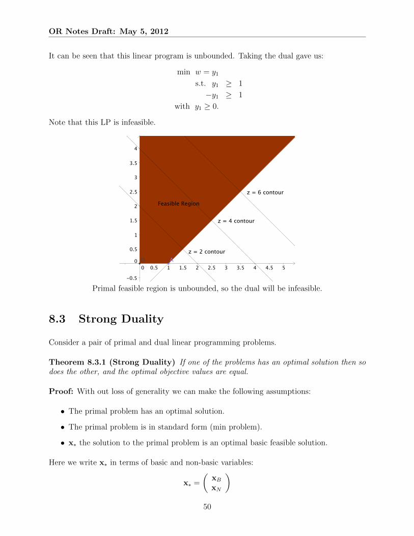
It can be seen that this linear program is unbounded. Taking the dual gave us:
min w = y1
s.t. y1 ≥ 1
−y1 ≥ 1
with y1 ≥ 0.
Note that this LP is infeasible.
Primal feasible region is unbounded, so the dual will be infeasible.
8.3 Strong Duality
Consider a pair of primal and dual linear programming problems.
Theorem 8.3.1 (Strong Duality) If one of the problems has an optimal solution then sodoes the other, and the optimal objective values are equal.
Proof: With out loss of generality we can make the following assumptions:
• The primal problem has an optimal solution.
• The primal problem is in standard form (min problem).
• x∗ the solution to the primal problem is an optimal basic feasible solution.
Here we write x∗ in terms of basic and non-basic variables:
x∗ =
(xBxN
)50

OR Notes Draft: May 5, 2012
and correspondingly we can write
A = [B N ], and c =
(cBcN
).
Recall any current basis may be written as:
xNT xB
T RHS Basis−cN
T + cBTB−1N 0 cB
TB−1b zB−1N I B−1b xB
Then we can note that xB = B−1b., and x∗ is optimal if
−cNT + cB
TB−1N ≤ 0 =⇒ cBTB−1N ≤ cN
T
the reduced costs for the non-basic variables are negative.
For the dual problem we let y∗ = (B−1)TcB.
y∗ = (B−1)TcB =⇒ y∗T = cTBB
−1
The goal now is to show that
• y∗ is feasible for the dual
• bTy∗ = cTx∗ (the objective functions have the same value).
For feasibility we need to show ATy∗ ≤ c. Lets start with
y∗TA = cTBB
−1(B N)
=(cTB cTBB
−1N)
≤(cTB cTN
)= cT
Thus,ATy∗ ≤ c
and we have a feasible solution for the dual.
We now need to compare the value of the dual’s objective function with the value of theoptimal primal objective function:
z = cTx∗ = cTBxB = cTBB−1b
w = bTy∗ = y∗Tb = cTBB
−1b
So y∗ is feasible in the dual and has the same objective value as the optimal primal problemobjective value so y∗ is optimal for the dual.
�
51

OR Notes Draft: May 5, 2012
More on Duality Theory
Primal Problem
Before starting into additional theory lets consider the following LP and for practice take itsdual.
min z = 20x1 + 15x2 + 54x3
s.t. x1 − 2x2 + 6x3 ≥ 30
x2 + 2x3 ≥ 6
2x1 − 3x3 ≥ −5
x1 − x2 ≥ 18
with x1, x2, x3 ≥ 0
The associated Dual problem is:
max w = 30y1 + 6y2 − 5y3 + 18y4
s.t. y1 + 2y3 + y4 ≤ 20
−2y1 + y2 − y4 ≤ 15
6y1 + 2y2 − 3y3 ≤ 54
with y1, y2, y3, y4 ≥ 0
Insight By Example
Lets consider working through an example start to finish in both the primal and dual for-mulation and see how the two are related.
Primal Problem:
min z = 2x1 + 9x2 + 3x3
s.t. − 2x1 + 2x2 + x3 ≥ 1
x1 + 4x2 − x3 ≥ 6
with x1, x2, x3 ≥ 0
Solving the Primal Problem
Adding excess variables and artificial variables to each of the primal constraints we mayobtain the following initial simplex tableau. Note we will use the two-phase simplex algorithm
52
OR Notes Draft: May 5, 2012
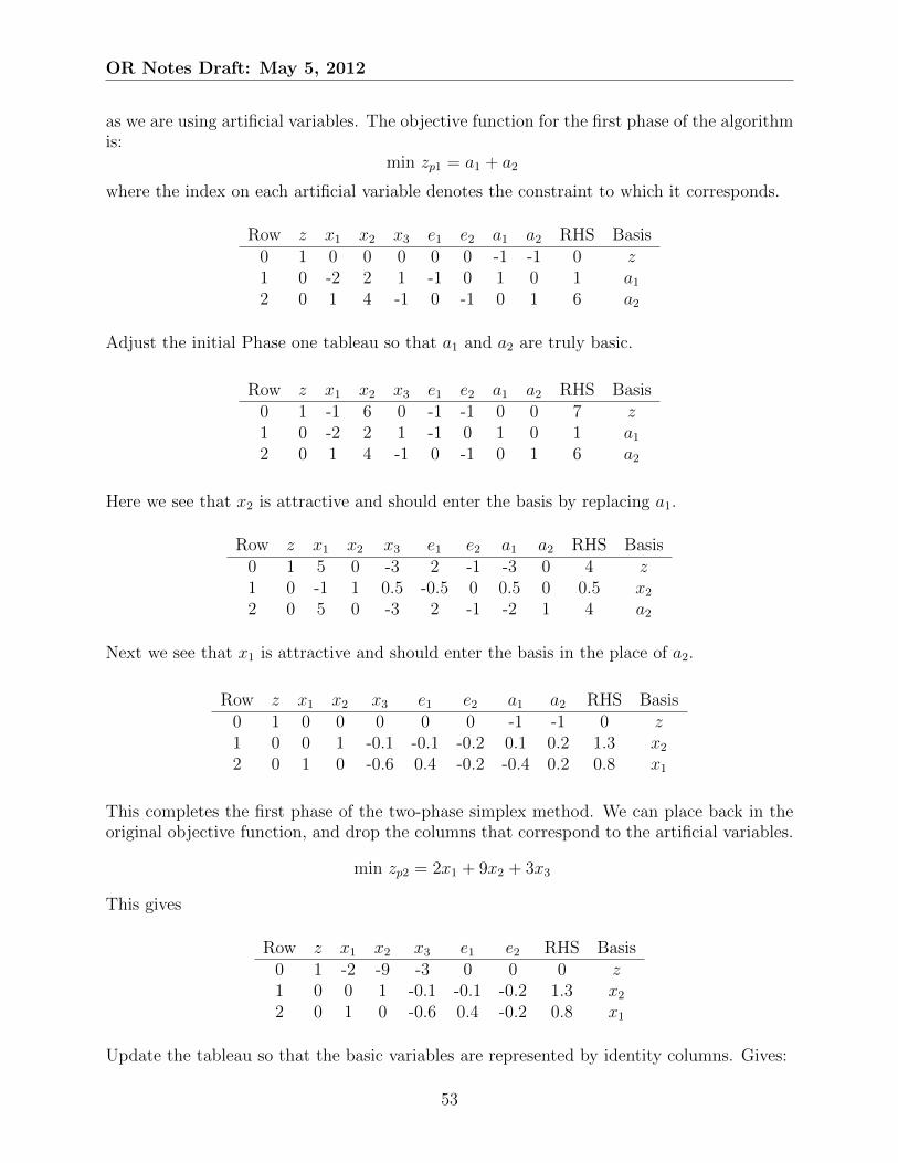
as we are using artificial variables. The objective function for the first phase of the algorithmis:
min zp1 = a1 + a2
where the index on each artificial variable denotes the constraint to which it corresponds.
Row z x1 x2 x3 e1 e2 a1 a2 RHS Basis0 1 0 0 0 0 0 -1 -1 0 z1 0 -2 2 1 -1 0 1 0 1 a1
2 0 1 4 -1 0 -1 0 1 6 a2
Adjust the initial Phase one tableau so that a1 and a2 are truly basic.
Row z x1 x2 x3 e1 e2 a1 a2 RHS Basis0 1 -1 6 0 -1 -1 0 0 7 z1 0 -2 2 1 -1 0 1 0 1 a1
2 0 1 4 -1 0 -1 0 1 6 a2
Here we see that x2 is attractive and should enter the basis by replacing a1.
Row z x1 x2 x3 e1 e2 a1 a2 RHS Basis0 1 5 0 -3 2 -1 -3 0 4 z1 0 -1 1 0.5 -0.5 0 0.5 0 0.5 x2
2 0 5 0 -3 2 -1 -2 1 4 a2
Next we see that x1 is attractive and should enter the basis in the place of a2.
Row z x1 x2 x3 e1 e2 a1 a2 RHS Basis0 1 0 0 0 0 0 -1 -1 0 z1 0 0 1 -0.1 -0.1 -0.2 0.1 0.2 1.3 x2
2 0 1 0 -0.6 0.4 -0.2 -0.4 0.2 0.8 x1
This completes the first phase of the two-phase simplex method. We can place back in theoriginal objective function, and drop the columns that correspond to the artificial variables.
min zp2 = 2x1 + 9x2 + 3x3
This gives
Row z x1 x2 x3 e1 e2 RHS Basis0 1 -2 -9 -3 0 0 0 z1 0 0 1 -0.1 -0.1 -0.2 1.3 x2
2 0 1 0 -0.6 0.4 -0.2 0.8 x1
Update the tableau so that the basic variables are represented by identity columns. Gives:
53

OR Notes Draft: May 5, 2012
Row z x1 x2 x3 e1 e2 RHS Basis0 1 0 0 -5.1 -0.1 -2.2 13.3 z1 0 0 1 -0.1 -0.1 -0.2 1.3 x2
2 0 1 0 -0.6 0.4 -0.2 0.8 x1
We have achieved the optimal solution to the primal linear programming problem. Theminimum is achieved when z = 13.3 with x1 = 0.8 and x2 = 1.3 and x3 = 0.
Solving the Dual Problem
The dual for our example problem is given by
max w = y1 + 6y2
s.t. − 2y1 + y2 ≤ 2
2y1 + 4y2 ≤ 9
y1 − y2 ≤ 3
with y1, y2 ≥ 0
Here we need to add a slack variable to each of the constraints. This leads to the initialtableau:
Row w y1 y2 s1 s2 s3 RHS Basis0 1 -1 -6 0 0 0 0 w1 0 -2 1 1 0 0 2 s1
2 0 2 4 0 1 0 9 s2
3 0 1 -1 0 0 1 3 s3
Note here we pick y2 to enter into the basis. It will replace s1.
Row w y1 y2 s1 s2 s3 RHS Basis0 1 -13 0 6 0 0 12 w1 0 -2 1 1 0 0 2 y2
2 0 10 0 -4 1 0 1 s2
3 0 -1 0 1 0 1 5 s3
Here we pick y1 to enter the basis in place of s2. This gives,
Row w y1 y2 s1 s2 s3 RHS Basis0 1 0 0 0.8 1.3 0 13.3 w1 0 0 1 0.2 0.2 0 2.2 y2
2 0 1 0 -0.4 0.1 0 0.1 y1
3 0 0 0 0.6 0.1 1 5.1 s3
The optimal solution has been obtained with w = 13.3 where y1 = 0.1 and y2 = 2.2.
54

OR Notes Draft: May 5, 2012
Observations
Note we could have solved the Dual problem graphically:
Lets compare the optimal Tableau for each of the two problems:
Row z x1 x2 x3 e1 e2 RHS Basis0 1 0 0 -5.1 -0.1 -2.2 13.3 z1 0 0 1 -0.1 -0.1 -0.2 1.3 x2
2 0 1 0 -0.6 0.4 -0.2 0.8 x1
PRIMAL
Row w y1 y2 s1 s2 s3 RHS Basis0 1 0 0 0.8 1.3 0 13.3 w1 0 0 1 0.2 0.2 0 2.2 y2
2 0 1 0 -0.4 0.1 0 0.1 y1
3 0 0 0 0.6 0.1 1 5.1 s3
DUAL
• Note we can read the primal and dual solutions for the other problem using the reducedcosts in row zero of the optimal tableau.
– The optimal dual variable values are the same as the reduced costs of the slack(and excess variables with with signs reversed).
55

OR Notes Draft: May 5, 2012
Complementary Slackness
The optimal solutions are given by:
PRIMAL =
x1
x2
x3
e1
e2
=
0.81.3000
and DUAL =
y1
y2
s1
s2
s3
=
0.12.200
5.1
We can line up the constraints and sign restrictions for each problem and note which one isbinding in each of the problems:
PRIMAL PROBLEM BINDING DUAL PROBLEM−2x1 + 2x2 + x3 ≤ 1 PRIMAL y1 ≥ 0x1 + 4x2 − x3 ≤ 6 PRIMAL y2 ≥ 0x1 ≥ 0 DUAL −2y1 + y2 ≤ 2x2 ≥ 0 DUAL 2y1 + 4y2 ≤ 9x3 ≥ 0 PRIMAL y1 − y2 ≤ 3
This illustrates complementary slackness.
Consider the primal-dual pair in standard form:
PRIMAL: min z = cTx
s.t. Ax = b
with x ≥ 0
DUAL: max w = bTy
s.t. ATy ≤ c
with y is free
There is an interdependence between the non-negativity constraints in the primal (x ≥ 0) andthe constraints in the dual (ATy ≤ c). At the optimal solution it is not possible to have both:
xj > 0 and (ATy)j < cj.
At least one of the constraints must be binding giving that either
• xj = 0 or
• the j-th dual slack variable is zero (the corresponding dual constraint is binding).
Note this gives that ∑j
xj(c− ATy)j
56

OR Notes Draft: May 5, 2012
Complementary slackness is often written as:
xT (c− ATy) = 0.
as the primal and dual constraints ensure that the terms in the summation must be non-negative. Thus, if the sum is zero then each term must be zero.
Theorem 8.3.2 (Complementary Slackness) Consider a pair of primal and dual linearprograms in standard form. If x is optimal for the primal and y is optimal for the dual then
xT (c− ATy) = 0
Proof: If x and y are feasible for there respective problems then:
z = cTx ≥ yTAx = yTb = w.
As x and y are also optimal we know that z = w so
cTx = yTAx =⇒ xTc = xTATy
=⇒ xTc− xTATy = 0
=⇒ xT(c− ATy
)= 0
�
8.4 The Dual Simplex Method
Consider the following linear program:
min z = 5x1 + 4x2
s.t. 4x1 + 3x2 ≥ 10
3x1 − 5x2 ≥ 12
with x1, x2 ≥ 0.
If we add excess variables to the constraints and place the problem into a tableau we have:
Row z x1 x2 e1 e2 RHS BASIS0 1 -5 -4 0 0 0 z1 0 4 3 -1 0 10 ?2 0 3 -5 0 -1 12 ?
Note that in the above Tableau we do not have any basic variables yet. However, thegiven tableau does show that the reduced costs for the problem are such that the optimalityconditions are satisfied. Lets consider making e1 and e2 basic (multiply row 1 and row 2 by-1). This gives the following tableau.
57

OR Notes Draft: May 5, 2012
Row z x1 x2 e1 e2 RHS BASIS0 1 -5 -4 0 0 0 z1 0 -4 -3 1 0 -10 e1
2 0 -3 5 0 1 -12 e2
Note that:
• The optimality conditions are still satisfied. (Nothing is attractive to enter into thebasis in the simplex method as we know it.)
• The right hand side values are negative. This means that he current basis is infeasiblein the primal problem.
To move toward a feasible solution we could scan the RHS and see who is the most negative,and work to get them out of the basis. Here we need a candidate to come in in thereplace. Scan down the row corresponding to the mose negative RHS value and find negativecoefficients. If there is more than one we would do a ‘Ratio’ test (reduced cost divided bythe exiting row coefficient in the potential entering column) taking the minimum value tobe our entering variable.
Row z x1 x2 e1 e2 RHS BASIS0 1 0 -37
30 -5
320 z
1 0 0 -293
1 -43
6 e1
2 0 1 -53
0 -13
4 x1
After doing the update we can now see that the optimality conditions and the primal feasi-bility conditions have now both been satisfied. Yielding the optimal solution of z = 20 whenx1 = 4 and x2 = 0. This technique is called the dual simplex method . We can verify thatthis is indeed the solution to the problem by considering it graphically.
58

OR Notes Draft: May 5, 2012
A Second Example
Use the dual simplex method to solve the following linear program:
min z = 5x1 + 2x2 + 8x3
s.t. 2x1 − 3x2 + 2x3 ≥ 3
−x1 + x2 + x3 ≥ 5
with x1, x2, x3 ≥ 0.
Setting up the problem in tableau form using two excess variables:
Row z x1 x2 x3 e1 e2 RHS BASIS0 1 -5 -2 -8 0 0 0 z1 0 2 -3 2 -1 0 3 ?2 0 -1 1 1 0 -1 5 ?
We negate the two constraints in order to make e1 and e2 basic.
Row z x1 x2 x3 e1 e2 RHS BASIS0 1 -5 -2 -8 0 0 0 z1 0 -2 3 -2 1 0 -3 e1
2 0 1 -1 -1 0 1 -5 e2
Here we look to get e2 out of the basis. We see that x2 is the winner of the Ratio Test.
Row z x1 x2 x3 e1 e2 RHS BASIS0 1 -7 0 -6 0 -2 10 z1 0 1 0 -5 1 3 -18 e1
2 0 -1 1 1 0 -1 5 x2
Note that after the pivot of the Dual Simplex algorithm there is no attractive candidate toenter into the basis using our normal “Primal Simplex” algorithm (the optimality conditionsare still met). We now use Dual simplex to remove e1 from the basis. Note that x3 is theonly choice to replace e1 in the basis.
Row z x1 x2 x3 e1 e2 RHS BASIS0 1 -8.2 0 0 -1.2 -5.6 31.6 z1 0 -0.2 0 1 -0.2 -0.6 3.6 x3
2 0 -0.8 1 0 0.2 -0.4 1.4 x2
Note that the optimal solution of z = 31.6 is achieved when x1 = 0, x2 = 1.4 and x3 = 3.6.
We make note here that the Dual Simplex method is especially useful when doing sensitivityanalysis. If a change in the right hand side value of a constraint is made this method can beused to update the current simplex solution to one that is feasible if the change causes theprimal problem to have negative right hand side values.
59
OR Notes Draft: May 5, 2012
60

Chapter 9
Sensitivity Analysis
“ I don’t know where the sun beams endand the star light begins it’s all a mystery...”
−The Flaming Lips
9.1 Sensitivity Analysis
Before looking at sensitivity analysis it is good to have a base problem to consider. We willbase our initial pilgrimage into sensitivity analysis of linear programs on the following 2Dlinear program.
Base Problem
Consider maximizing the profit from manufacturing two items on three different assemblylines. The profit from manufacturing item 1 is three thousand dollars, and from item 2 is fivethousand dollars. Letting x1 and x2 be the number of each of these items to manufacture,and letting the following constraints denote the number of hours that it takes to manufactureeach of the items at three different assembly lines with the given restrictions on the maximumnumber of hours available on each line. This gives the following linear program:
maximize z = 3x1 + 5x2
subject to x1 ≤ 42x2 ≤ 12
3x1 + 2x2 ≤ 18x1, x2 ≥ 0.
Assuming you are renting time on each assembly line what is the most you should pay foran additional hour of time on each of the assembly lines?
61

OR Notes Draft: May 5, 2012
Solution:Using the simplex algorithm to solve the given linear program we see that after adding twoslack variables in the constraints the initial tableau for the given linear program is writtenas:
Row z x1 x2 s1 s2 s3 RHS Basis0 1 -3 -5 0 0 0 0 z1 0 1 0 1 0 0 4 s1
2 0 0 2 0 1 0 12 s2
3 0 3 2 0 0 1 18 s3
Here it becomes desirable to pivot x2 into the basis replacing s2. Thus,
Row z x1 x2 s1 s2 s3 RHS Basis0 1 -3 0 0 5
20 30 z
1 0 1 0 1 0 0 4 s1
2 0 0 1 0 12
0 6 x2
3 0 3 0 0 -1 1 6 s3
The next iteration of the simplex method shows that it is desirable to have x1 inter the basisand it will replace s3. Doing this pivot yields:
Row z x1 x2 s1 s2 s3 RHS Basis0 1 0 0 0 3
21 36 z
1 0 0 0 1 13
-13
2 s1
2 0 0 1 0 12
0 6 x2
3 0 1 0 0 -13
13
2 x1
Here we have obtained an optimal tableau. We can see here that profit is maximized at$36,000 when x1 = 2 and x2 = 6 are manufactured between the different assembly lines.
Shadow prices:
We are often interested in the marginal value of each of the given resources and their impacton the objective function. That is:
Shadow Price : measures the marginal value of a given resource or the amountby which z will be increased by slightly increasing the amount of a given resourcebeing made available.
The shadow price for resource i is denoted by y∗i and is the amount the objective function willbe increased if the amount of resource bi is slightly increased. The shadow price for resourcei is the zero row coefficient for the ith constraints slack variable in the optimal tableau.
62

OR Notes Draft: May 5, 2012
From our given example we can see that the shadow price for hours available for eachassembly line (marginal increase in the objective function for slight increases in the amountthe resource available) is:
y∗1 = 0, y∗2 =3
2y∗3 = 1. (9.1.1)
9.1.1 Verify this graphically:
An interactive version of the solution is found at:
http://www.math.iup.edu/~jchrispe/MATH445_545/ShadowPrices.html
What happens if the constraint b2 goes from 12 to 13?
y∗2 = ∆z = 37.5− 36 = 1.5 (9.1.2)
How do we interpret this with regard to the linear program?
An additional unit of labor on production line two will increase the profits by$1500.
How far could we increase the value of b2 the amount of resource 2 and still stay optimalwith the current basis?
63

OR Notes Draft: May 5, 2012
We could increase the units of resource b2 up to 18 and keep the same basicfeasible solution. After which the constraint is no longer binding. Here theoptimal objective function would be fixed at z =45. At this point a new basicfeasible solution can be obtained, and a new set of shadow prices will come intoplay.
Note that constraints that have zero shadow prices are not binding the objective function.In the given example we note that the first constraint is not binding and increasing the valueof b1 will have no effect on the objective function’s optimal value. Resources for bindingconstraints are sometimes called scarce goods, and resources for non-binding constraintsare called free goods.
• Shadow prices can be also thought of as the maximum price you would want to payfor an additional unit of a given resource.
• Shadow prices help identify the parameters in the model that need to be estimatedcarefully. If a shadow price is zero the model is not sensitive to (at least small) changesin the given resource.
• You would want to monitor resources more closely if they have large shadow prices.
How far can b2 be changed and keep the same optimal basic feasible solution?
6 ≤ b2 ≤ 18
keeps the same basic feasible solution, and an increase of 6 or a decrease of 6 is allowed.What information can we get out of LINDO/LINGO?
9.2 Sensitivity Analysis Using Matrices
We looked briefly as sensitivity of linear programs graphically. This is nice if the problem issmall enough to handle with a software like Geogebra. However; it becomes more difficult todetermine how the solution to a linear program is effected by perturbations of the objectivefunction coefficients and constraints if the problem of interest is more than two dimensional.
Lets recall that for a linear program in the form:
(min or max) cTx
s.t. Ax = b
with x ≥ 0
then any current basis may be written using matrix form (using our previously definednotation) as:
xNT xB
T RHS Basis−cN
T + cBTB−1N 0 cB
TB−1b zB−1N I B−1b xB
64
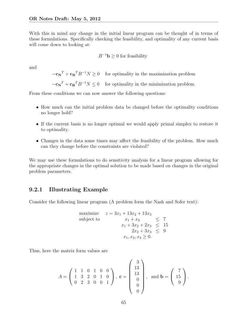
OR Notes Draft: May 5, 2012
With this in mind any change in the initial linear program can be thought of in terms ofthese formulations. Specifically checking the feasibility, and optimality of any current basiswill come down to looking at:
B−1b ≥ 0 for feasibility
and
−cNT + cB
TB−1N ≥ 0 for optimality in the maximization problem
−cNT + cB
TB−1N ≤ 0 for optimality in the minimization problem.
From these conditions we can now answer the following questions:
• How much can the initial problem data be changed before the optimality conditionsno longer hold?
• If the current basis is no longer optimal we would apply primal simplex to restore itto optimality.
• Changes in the data some times may affect the feasibility of the problem. How muchcan they change before the constraints are violated?
We may use these formulations to do sensitivity analysis for a linear program allowing forthe appropriate changes in the optimal solution to be made based on changes in the originalproblem parameters.
9.2.1 Illustrating Example
Consider the following linear program (A problem form the Nash and Sofer text):
maximize z = 3x1 + 13x2 + 13x3
subject to x1 + x2 ≤ 7x1 + 3x2 + 2x3 ≤ 15
2x2 + 3x3 ≤ 9x1, x2, x3 ≥ 0.
Thus, here the matrix form values are
A =
1 1 0 1 0 01 3 2 0 1 00 2 3 0 0 1
, c =
3
1313000
, and b =
7159
.
65

OR Notes Draft: May 5, 2012
If the optimal solution to the problem is found the optimal basis xB = (x1 x2 x3)T , andxN = (s1 s2 s3)T we have:
N =
1 0 00 1 00 0 1
, B =
1 1 01 3 20 2 3
=⇒ B−1 =
52−3
21
−32
32−1
1 −1 1
.
with
cNT =
(0 0 0
)cB
T =(
3 13 13)
Lets answer the following questions:
1. What is the solution to the problem?Where we find the values of the decision variables as:
Current RHS B−1b =
52−3
21
−32
32−1
1 −1 1
7159
=
431
.
Objective Value cBTB−1b =
(3 13 13
) 431
=(
64)
Thus, x1 = 4, x2 = 3, and x3 = 1.
2. What are the optimal dual variables?
Dual Variables − cNT + cB
TB−1N
=(
0 0 0)
+(
3 13 13) 5
2−3
21
−32
32−1
1 −1 1
1 0 00 1 00 0 1
=
(1 2 3
)Note these are the shadow prices, and if the problem had more context they would tellus the most we would wish to pay for an additional unit on the right hand side of eachof the constraints.
3. What is the solution obtained by decreasing the right-hand side of the second constraintby 5?
Now we add a vector of the form: ∆b = (0,−5, 0)T to the initial b vector:
bnew =
7159
+
0−5
0
=
7109
.
66

OR Notes Draft: May 5, 2012
Where we find the values of the decision variables as:
Current RHS B−1b =
52−3
21
−32
32−1
1 −1 1
7109
=
232
−92
6
.Thus, x1 = 23
2, x2 = −9
2, and x3 = 6. Here the RHS is no longer feasible for the
problem as x2 < 0. So we can implement an iteration of the dual simplex methodto find a new basic feasible solution. We need to have a handle on the values of thenon-basic columsn which are given by
Non-Basic Columns B−1N =
52−3
21
−32
32−1
1 −1 1
as well as the new values for the dual variables:
Dual Variables − cNT + cB
TB−1N =(
1 2 3)
We do the Ratio Test for an iteration of the dual simplex method giving:
min
{col1 =
∣∣∣∣ 1−32
∣∣∣∣ =2
3, col3 =
∣∣∣∣ 3
−1
∣∣∣∣ = 3
}So we pick x2 to leave the basis and we choose s1 to enter. This gives the new optimalsolution to be: xB = (x1 s1 x3)T , and xN = (x2 s2 s3)T
Where we now have:
B =
1 1 01 0 20 0 3
and N =
1 0 03 1 02 0 1
.
Dual Variables − cNT + cB
TB−1N =(
23
3 73
)Current RHS B−1b =
433
.Objective Value cB
TB−1bnew =(
51)
4. By how much can the right-hand side of the first constraint increase and decreasewithout changing the optimal basis?
67

OR Notes Draft: May 5, 2012
Here we are looking at the first component of B−1(b+ b∆) and want to see what rangeof values will keep the first component non-negative where:
b∆ =
∆b00
Thus,
B−1 (b + b∆) =
52−3
21
−32
32−1
1 −1 1
7 + ∆b159
=
52
(7 + ∆b)− 32(15) + (9) ≥ 0
−32
(7 + ∆b) + 32(15)− (9) ≥ 0
(7 + ∆b)− (15) + (9) ≥ 0
These constraints lead to the following conditions:
∆b ≥ −8
5,∆b ≤ 2 , and ∆b ≥ −1.
so the right hand side of the first constraint may increase by at most 2, and decreaseby at most 1 with out changing the current basis.
5. What is the optimal solution to the linear program obtained by increasing the coeffi-cient of x2 in the objective function by 15? Here the value of
cB =
32813
For the different components of the problem we see that:
Objective Value cBTB−1b =
(109
),
The values of the decision variables are:
Current RHS B−1b =
431
.Thus, x1 = 4, x2 = 3, and x3 = 1, and the current dual variables
Dual Variables − cNT + cB
TB−1N =(−43
2492−12
)As we now have an attractive entering variable we can do a Primal simplex pivot withs1 entering the basis. The ratio test using:
Current Non-Basic Columns B−1N =
52−3
21
−32
32−1
1 −1 1
68

OR Notes Draft: May 5, 2012
and the Current RHS yields that x3 should leave the basis. This gives xB = (x1 x2 s1)T ,and xN = (x3 s2 s3)T where
N =
0 0 02 1 03 0 1
and B =
1 1 11 3 00 2 0
We can look at the updated dual variables and see that:
Objective Value cBTB−1b =
(2612
),
The values of the decision variables are:
Current RHS B−1b =
3292
1
.Thus, x1 = 3
2, x2 = 9
2, and x3 = 0, and the current dual variables are
Dual Variables − cNT + cB
TB−1N =(
432
3 192
)Note that as the dual variable corresponding to s3 is zero it is also a potential candidateto enter the basis giving us multiple optimal solutions.
6. How much can the objective coefficient of x1 increase and decrease without changingthe optimal basis?Here we consider the value of the dual variables that is:
Dual Variables − cNT + cB
TB−1N =(
1 2 3)
Note that cN =(
0 0 0)
so we need only consider the following:
((3 + ∆c) 13 13)
52−3
21
−32
32−1
1 −1 1
1 0 00 1 00 0 1
≥ 0
=⇒ ((3 + ∆c) 13 13)
52−3
21
−32
32−1
1 −1 1
≥ 0
=⇒ 5
2(3 + ∆c) + (13)(
−3
2) + (13) ≥ 0,
−3
2(3 + ∆c) + (13)(
3
2)− (13) ≥ 0,
(3 + ∆c)− 13 + (13) ≥ 0
This gives that
x ≥ −2
5, x ≤ 4
3, and x ≥ −3.
so the coefficient on x1 in the objective function can be increased by at most 43
and
decreased by at most 25
if the same optimal basis is to be maintained.
69

OR Notes Draft: May 5, 2012
70

Chapter 10
Non Linear Programming
“ “Our opponent is an alien starship packed with atomic bombs,” I said. “We have aprotractor.” ”
−Neal Stephenson, Anathem
There are many instances where the problem considered involves more that a linear rela-tionship between decision variables and our objective. Here we will examine some of thepreliminaries of non-linear programming starting with fitting functional models to sets ofdata.
10.1 Data Fitting
There are many instances where it would be advantageous to find a best fit model for a set ofdata. Here we have a set of points and we want to find in some sense the model or functionthat “best fits” the set of points 1.
For us best fit will be in the least squares sense. Thus given a set of n points (ti, yi), wewant to find a vector of m parameters x that will minimize the least square residual of:
minimize
x
n∑i=1
(yi − f(ti,x))2 ,
where
f : Rm+1 → R.
This may be a linear or non-linear problem depending on whether the function f is linear inits components of the parameter vector x.
1Here we will follow the presentation in Heath’s Text.
71

OR Notes Draft: May 5, 2012
10.1.1 Linear Problems
Consider for example where we are interested in finding a function:
f(t,x) = x1 + x2t+ x3t2 + . . .+ xmt
m−1
that best fits our set of n points we have to find the m coefficients for vector x that wouldminimize our residual in the least squares sense described above.
This problem and others where the parameters x in f are linear combinations will result ina matrix system of the form
Ax ∼= b.
Lets work a couple of examples.
Example:
Consider finding the best fitting linear and quadratic function for the following set of points:
(1, 0), (2, 5), (3, 8), (4, 17), (5, 24)
For the case of a linear function we want to find values of x = (x1, x2)T in
f(t,x) = x1 + x2t
such that we minimize the sum of
min5∑i=1
yi − f(ti,x)
Writing this out as a matrix system:
Ax =
1 t11 t21 t31 t41 t5
[x1
x2
]∼=
y1
y2
y3
y4
y5
= b.
Or with our given set of points:
Ax =
1 11 21 31 41 5
[x1
x2
]∼=
058
1724
= b.
So a residual vector could be found by looking at
r = b− Ax
72

OR Notes Draft: May 5, 2012
if we are going look at the minimum of squared Euclidean norm of this residual can considerfinding the minimum of
φ(x) = ‖r‖22
= rT r
= (b− Ax)T (b− Ax)
= bTb− bTAx− (Ax)Tb + (Ax)T (Ax)
= bTb− 2bTAx + xTATAx
If we use methods from multi variable calculus we know that the residual function will havea potential minimum provided (necessary condition):
∇φ(x) = 0
Thus, we will consider:
0 = ∇φ(x)
= 0− 2bTA+ ATAx + ATAx
= −2bTA+ 2ATAx
=⇒ ATAx = ATb
For this to indeed be a minimum note that we need the Hessian Matrix (matrix of secondpartial derivatives) given by ATA to be positive definite. (This can be proved by showingthat ATA has rank n or that the columns are linearly independent). Note this system ofequations is known as the Normal Equations.
Looking back at our example we need to consider:(5 15
15 55
)[x1
x2
]=
(54
222
)And solving the equation gives:
x =
[x1
x2
]=
(−36
5
6
)So the minimizing linear function is given by:
f(t) = 6t− 36
5
and we make note that if we evaluate φ(x) gives:
φ(x) = bTb− 2bTAx + xTATAx = 10.8
73

OR Notes Draft: May 5, 2012
Now lets consider fitting a quadratic function to the data. Thus we want to find the best fitfunction of the form:
f(t,x) = x1 + x2t+ x3t2
The new system matrix is:
Ax =
1 t1 t211 t2 t221 t3 t231 t4 t241 t5 t25
x1
x2
x3
∼=y1
y2
y3
y4
y5
= b.
After substituting our point into the matrix A we have:
Ax =
1 1 11 2 41 3 91 4 161 5 25
[x1
x2
]∼=
058
1724
= b.
x =
x1
x2
x3
=
−11512757
Thus, the best fit quadratic function for the set of points is given by
f(t) =5
7t2 +
12
7t− 11
5
Plotting our two found functions and the original data set gives:
74

OR Notes Draft: May 5, 2012
Non-linear Problems
In order to consider non linear problems we need to consider iterative methods that will helpus find the optimal solution to our data fitting problem.
10.1.2 Taylor series
Lets recall in one dimension that we can expand a function about a close point (x + h)provided we know information about our function at point x. Thus a Taylor series expansionis:
f(x+ h) =f(x)
0!+f ′(x)h
1!+f ′′(x)h2
2!+ · · ·
Truncate the expansion after the first term gives:
f(x+ h) ≈ f(x) + f ′(x)h
For a numerical scheme we could note that h is the distance between to points:
h = x1 − x
Thus, we can make a note that an approximation of the first derivative can be given by:
f(x+ x1 − x) ≈ f(x) + f ′(x)(x1 − x)
=⇒ f ′(x) ≈ f(x1)− f(x)
(x1 − x)
10.1.3 Newton’s Method
Newton’s method is a way of iterating toward the root a function given that you have aninitial guess that is reasonably close to the root. To find the root of
f(x) = 0
we guess that x1 is our root. Then an iterative scheme for approaching a root would begiven by rearranging the first derivative approximation that we just found (with f(x1) ≈ 0)to obtain:
xn = xn−1 −f(xn−1)
f ′(xn−1)
where we iterate from some initial guess until some predetermined tolerance is achieved.
In order to solve non-linear equations in multiple dimensions we can look at a generalizationof Newton’s Method. Looking at a function f such that f : Rn → Rn, the truncated Taylorseries expansion is given by:
f(x + s) ≈ f(x) + Jf (x)s (10.1.1)
75

OR Notes Draft: May 5, 2012
where we are using Jf (x) to denote the Jacobian matrix of x. Specifically,
Jf (x)i,j =∂fi(x)
∂xj.
Noting that s is given as:s = xn − x =⇒ xn = s + x
and that xn is an approximate zero to f , we can rewrite (10.1.1) as:
xn ≈ x− f(x)
Jf (x)
An algorithm for solving a system of f(x) = 0 for some initial guess x0 could be written inthe following manner:
Algorithm for Newton’s Method (System of non-linear equations):
While ‖s‖2 > tolerance.
• Solve Jf (xn−1)sn = −f(xn−1) for sn.
• Update xn = xn−1 + sn
Lets now consider newtons method for a function f : Rm → R. Here a two term in ourTaylor series expansion:
f(x + s) ≈ f(x) +∇f(x)T s +1
2sTHf (x)s.
where Hf (x) is the Hessian matrix of second partial derivatives of f such that:
Hf (x)i,j =∂2f(x)
∂xi∂xj
It follows that the function f(x + s) will have a minimum when
Hf (x)s = −∇f(x). (10.1.2)
To see this you should look at this as if f is a quadratic function in s, and note that (10.1.2)is the vertex of the function. This allows us the oppertunity to think of Newton’s Methodas:
Algorithm for Newton’s Method :
While ‖s‖2 > tolerance.
• Solve Hf (xn−1)sn = −∇f(xn−1) for sn.
• Update xn = xn−1 + sn
76

OR Notes Draft: May 5, 2012
10.2 Non-linear Least Squares
Lets start by considering a biological system that involves fitting parameters to a mathe-matical model of a swimming lamprey. The work of Dr. Chia-Yu Hsu involves numericalsimulations of these swimmers:
http://www.ccs.tulane.edu/~chiayu/
Here the goal will be to fit a set of swimming data with a best fit model of the followingform:
f(x, t) = (ax2 + bx+ c) sin(kx+ ωt)
where we need to find the values of a, b, c, k, and ω that will best fit our model.
In order to solve this problem lets assume that we are given a set of m points of the form(ti, yi) and we want to fit a nonlinear function with vector of parameters x ∈ Rk such thatthe function f(t,x), is the best fit to the given data set where f : Rk+1 → R. Thus, our goalis to minimize the residual r where r : Rk → Rm, and
ri(x) = yi − f(ti,x), for i ∈ {1, 2, . . . ,m}.
where we are now hoping to minimize
φ(x) =1
2‖r‖2
2 =1
2r(x)T r(x).
We have placed the 12
into the function φ for convenience. In order to apply Newton’s Methodto this problem we need to find the following components:
∇φ(x), and Hφ(x).
Finding the first of these expressions is not troubling. Denote the Jacobian matrix of r(x)by J(x) gives
∇φ(x) = JT (x)r(x).
For the second term we calculate the Hessian Matrix of φ as
Hφ(x) = JT (x)J(x) +m∑i=1
ri(x)Hri(x).
Calculating the Hri(x) is often difficult and computationally expensiveso it is often ignoredor dropped fom computations. The result in what is known as a Gauss-Newton Methodgiven by:
Algorithm for Newton’s Method :
While ‖s‖2 > tolerance.
77

OR Notes Draft: May 5, 2012
• Solve JT (xn−1)J(xn−1)sn = −JT (xn−1)r(xn−1) for sn.
• Update xn = xn−1 + sn
Note the solve step looks like the normal equations for a nonlinear least squares problem.
The question now is what does J(x) look like for our given problem? This is the Jacobeanmatrix of the residual vector. For the swimmers we have:
f(x, x, t) = (ax2 + bx+ c) sin(kx+ ωt)
where we need to find the values of a, b, c, k, and ω that will best fit our model to a givenset of data along a swimmer. Lets let φ = ωt be a parameter all by itself and then back thevalue of ω out of the time dependent data fit (as we are doing this for a moving swimmer).Thus,
f(x, x) = (ax2 + bx+ c) sin(kx+ φ), and x = (a, b, c, k, φ)T
So at any time we are looking at the residual vector for our m points where the componentsof r(x) are:
ri(x) = yi − f(x, ti) for i ∈ {1, 2, . . . ,m}.
and the components of the residuals Jacobean are
J(x)i,1 =∂ri(x)
∂a= −(t2i ) sin(kti + φ)
J(x)i,2 =∂ri(x)
∂b= −ti sin(kti + φ)
J(x)i,3 =∂ri(x)
∂c= − sin(kti + φ)
J(x)i,4 =∂ri(x)
∂k= −(at2i + bti + c) cos(kti + φ)ti
J(x)i,5 =∂ri(x)
∂φ= −(at2i + bti + c) cos(kti + φ)
At the end of the day we will have a five by five matrix system to iterate on and find ouroptimal parameters. Note as we are going to solve this over different time sets we will beable to plot the value computed for φ as a function of the different input times and back outa value for ω the speed of the swimmer.
78
Chapter 11
Network Flows
“It’s hard to decide who’s truly brilliant; it’s easier to see who’s driven, which in thelong run may be more important.”
−Michael Crichton
In this chapter a collection of Network Algorithms will be examined. The current treatmentwill only serve to illustrate some of the other areas that can be explored in the world ofOperations Research.
11.1 Dijkstra’s Algorithm
Dijkstra’s Algorithm Can be used to find the shortest path spanning tree for a given network.Essentially the algorithm follows the following steps:
1. Set the distance to notes.
(a) The starting (or current) node distance is set to zero,
(b) All other nodes in the network are set to a distance of ∞.
2. Create a list of the unvisited nodes. Consisting of all nodes.
3. From the current node:
Consider the distance to all the unvisited node neighbours in the network.If the distance from the current node to the neighbour is less than the listedvalue in you “distance list” update the distance and the predecessor array.
4. Mark the current node as visited by removing from “unvisited list”.
5. If the distance to all unvisited nodes is∞ stop. Otherwise choose the closest unvisitednode to be the current node, and go back to step 3.
79

OR Notes Draft: May 5, 2012
Lets consider the algorithm with the following example:
Example:
Use Dijkstra’s algorithm to find a shortest path tree rooted at node 1 in the network below.Note that two of the arcs are bi-directional. Show at each iteration D(·), pred(·), and theselected node i∗ , as well as the final shortest path tree.
����
����
������
������
����
����>
-
QQQQs
- ����>
ZZZZ~
6
? ?��������6
@@@@@@@R
5
32
4
6
1
6
5
2
2
11
8
5
3
3
����
����5∞ ∞
���� ��
��
������
������>-
QQQQs
- ����>
ZZZZ~
6
? ?��������6
@@@@@@@R
Initialize
3
5
32
4
6
1
62
2
11
8
5
3
∞ ∞
∞
node 1∗ 2 3 4 5 6D( ) 0 ∞ ∞ ∞ ∞ ∞
pred( )
Note: The ∗ denotes the node selected and p will denote a nodes predecessor.
����
����
���� ��
��
����
����
����
���� ��
������
����
����
-
- ����>
ZZZZ~
6
? ?��������6
@@@@@@@R
QQQQs
����>
-
����>
ZZZZ~
? ?
6@@@@@@@R
����>6
��������
-
QQQQs3
5
32
4
6
1
62
2
11
8
5
3
∞
5 ∞6
3
∞
3
5
32
4
6
1
62
2
11
8
5
3
5
3
4
8
11
∞
node 1p 2 3 4 5 6∗
D( ) 0 6 ∞ ∞ ∞ 3pred( ) 0 1 1
node 1 2∗ 3 4 5 6p
D( ) 0 4 11 ∞ 8 3pred( ) 0 6 6 6 1
���� ��
��������
��
����
����
���� ��
������
����
����
����
����>
ZZZZ~
?
6����>
��������
-
QQQQs
6@@@@@@@R
-
?
ZZZZ~
?
����>
��������
QQQQs
6
-
?
6
����>
-
@@@@@@@R3
5
32
4
6
1
62
2
11
8
5
3
5
3
4 9
7
∞
3
5
32
4
6
1
62
2
11
8
5
3
5
3
4
7
8
9
80
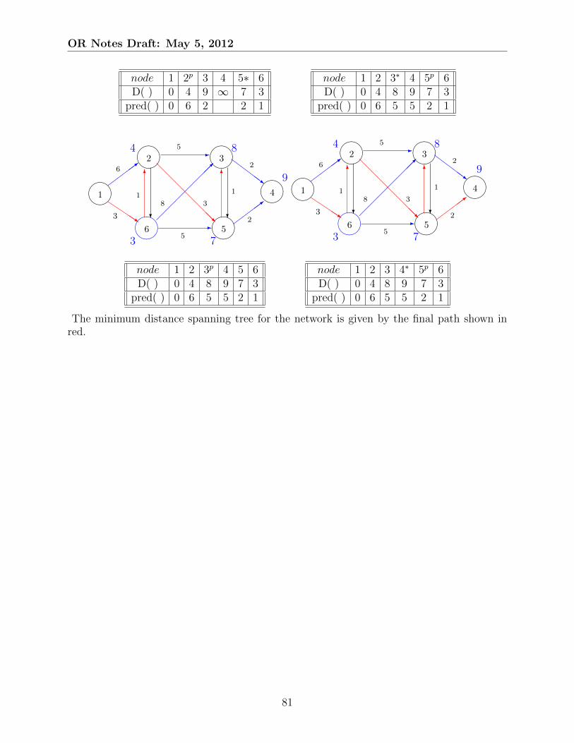
OR Notes Draft: May 5, 2012
node 1 2p 3 4 5∗ 6D( ) 0 4 9 ∞ 7 3
pred( ) 0 6 2 2 1
node 1 2 3∗ 4 5p 6D( ) 0 4 8 9 7 3
pred( ) 0 6 5 5 2 1
����
����
����
����
����
����
?
����>
��������
QQQQs
6
-
?����>
-
@@@@@@@R
6
ZZZZ~
3
5
32
4
6
1
62
2
11
8
5
3
5
3
4
7
8
9
����
����
����
����
����
����
?
����>
��������
QQQQs
6
-
?-
@@@@@@@R
6
����>
ZZZZ~
3
5
32
4
6
1
62
2
11
8
5
3
5
3
4
7
8
9
node 1 2 3p 4 5 6D( ) 0 4 8 9 7 3
pred( ) 0 6 5 5 2 1
node 1 2 3 4∗ 5p 6D( ) 0 4 8 9 7 3
pred( ) 0 6 5 5 2 1
The minimum distance spanning tree for the network is given by the final path shown inred.
81

OR Notes Draft: May 5, 2012
82

Chapter 12
Appendices
“Can you still have any famous last words if you’re somebody nobody knows?”
− Ryan Adams
12.1 Homework 1
Answer the following questions. Please include the questions with the solution. I do notwant to see scrap work.
1. Only three brands of beer (beer1, beer2, and beer3) are available for sale in Metropolis.From time to time, people try one or another of these brands. Suppose that at thebeginning of each month, people change the beer they are drinking according to thefollowing rules:
• 30% of the people who prefer beer 1 switch to beer 2.
• 20% of the people who prefer beer 1 switch to beer 3.
• 30% of the people who prefer beer 2 switch to beer 3.
• 30% of the people who prefer beer 3 switch to beer 2.
• 10% of the people who prefer beer 3 switch to beer 1.
For i = 1, 2, 3, let xi be the number who prefer beer i at the beginning of this monthand let yi denote the number who prefer beer i at the beginning of next month. Usematrix notation to relate x = (x1 x2 x3)T and y = (y1 y2 y3)T . Note that the followingequations will hold for the rules given above:
0.5x1 + 0.0x2 + 0.1x3 = y1 People switch to beer 1
0.3x1 + 0.7x2 + 0.3x3 = y2 People switch to beer 2.
0.2x1 + 0.3x2 + 0.6x+ 3 = y3 People switch to beer 3.
83
where we needed to find the number of people that stayed loyal to any particular typeover the course of the month. Let
A =
0.5 0.0 0.10.3 0.7 0.30.2 0.3 0.6
.and note that
Ax = y.
2. Show that for any two matrices A and B, (AB)T = BTAT .Assume that A is an m× n matrix and B is an n× q matrix so that there product isdefined. Thus, AB is an m × q matrix, and its transpose is a q ×m matrix. We canalso note that BTAT is the product q×n matrix and a n×m matrix resulting in againa q ×m. So each side of the equality is of the same size. We now only need to showthat the arbitrary element in row i and column j of (AB)T is the same as the row icolumn j element in BTAT .
Denoting the entry in row i column j in a matrix M as Mi,j we can consider thefollowing algebra:
(AB)Ti,j = (AB)j,i
=n∑k=1
Aj,kBk,i
=n∑k=1
ATk,jBTi,k
=n∑k=1
BTi,kA
Tk,j
= (BTAT )i,j
which concludes the proof.
3. Model each of the following decision making situations as a linear program(LP). Foreach LP clearly define your decision variables, objective function and constraints.
(a) Suppose that the latest scientific studies indicate that cattle need certain amountsb1, . . . , bm of nutrients N1, . . . , Nm respectively. More over, these nutrients are cur-rently found in n commercial feed materials F1, . . . , Fn as indicated by coefficientsaij, i = 1, . . . ,m, j = 1, . . . , n, that denote the number of units of nutrientNi perpound of feed material Fj. Each pound of Fj costs the rancher cj dollars. Howcan a rancher supply these minimal nutrient requirements to his prize bull whileminimizing his feed bill?
Linear Program: The goal of the problem is to minimize the cost of the bullsfood while maintaining the bulls healthy diet.

OR Notes Draft: May 5, 2012
Let xj be the number of pounds that the farmer should purchase of commercialfeed Fj where , j = 1, . . . , n. Thus the farmer wishes to minimize the followingcost equation (where z denotes the farmers total cost):
Minimize: z = c1x1 + c2x2 + . . .+ cnxn =n∑j=1
cjxj
In order to meet the nutrient requirments the farmer needs to impose the followingconstrictions on his cost equation:
a11x1 + a12x2 + a13x3 + . . . + a1nxn ≥ b1
a21x1 + a22x2 + a23x3 + . . . + a2nxn ≥ b2
a31x1 + a32x2 + a33x3 + . . . + a3nxn ≥ b3...
......
. . ....
...am1x1 + am2x2 + am3x3 + . . . + amnxn ≥ bm
where xj ≥ 0, j = 1, . . . , n
Let x = [x1, x2, · · · , xn]T , and c = [c1, c2, · · · , cn]T . We can also denote [b1, b2, · · · , bm]T
by b, and coefficient matrixa11 a12 a13 . . . a1n
a21 a22 a23 . . . a2n
a31 a32 a33 . . . a3n...
......
. . ....
am1 am2 am3 . . . amn
by A.
Thus the farmer is minimizing z = cTx subject to,
Ax ≥ b
where xj ≥ 0, j = 1, . . . , n
(b) Suppose that a small chemical company produces one chemical product which itstores in m storage facilities and sells in n retail outlets. The storage facilities arelocated in different communities. The shipping costs from storage facility Fi toretail outlet Oj is cij dollars per unit of the chemical product. On a given day,each outlet Oj requires exactly dj units of the product. Moreover, each facility Fihas si units of the product available for shipment. The problem is to determinehow many units of the product should be shipped from each storage facility toeach outlet in order to minimize the total daily shipping costs.
Linear Program: The goal of the problem is to minimize the cost of productshipping while maintaining product invintory and not overdrawing from supply.
Let xij be the number of units of chemical shipped from facility Fi to retail outletOj, where i ∈ {1, . . . ,m}, and j ∈ {1, . . . , n}. Let z denote the total cost of
85

OR Notes Draft: May 5, 2012
shipping. Thus, the chemical company wishes to optimize the followin objectivefunction,
Minimize: z =m∑i=1
n∑j=1
cijxij
In minimizing the above equation the company must meet the following con-straints:
x11 + x21 + . . .+ xm1 =∑m
i=1 xi1 ≥ d1
x12 + x22 + . . .+ xm2 =∑m
i=1 xi2 ≥ d2...
......
x1n + x2n + . . .+ xmn =∑m
i=1 xin ≥ dn
That is each outletj requires dj of chemical where j ∈ {1, . . . , n}. Each Facility ialso only has a limited supply of the chemical it can ship si where i ∈ {1, . . . ,m}.Thus, the problem has the constrictions:
x11 + x12 + . . .+ x1n =∑n
j=1 x1j ≤ s1
x21 + x22 + . . .+ x2n =∑n
j=1 x2j ≤ s2
......
...xm1 + xm2 + . . .+ xmn =
∑nj=1 xmj ≤ sm
where xij ≥ 0 , i ∈ {1, . . . ,m} and j ∈ {1, . . . , n}
The notation of the problem can be simplified if matrix notation is used:x11 x12 x13 · · · x1n
x21 x22 x23 · · · x2n...
......
. . ....
xm1 xm2 xm3 · · · xmn
= X
d1
d2...dn
= d, and
s1
s2...sm
= s.
Denote a column of 1’s that is k rows long by 1k and he linear program can nowtake the following form:
Minimize: z =m∑i=1
n∑j=1
cijxij
Subject to: X1n ≤ sXT1m ≥ d
where all elements of X are greator than or equal to zero.
86

OR Notes Draft: May 5, 2012
(c) An investor has decided to invest a total of $50,000 among three investment op-portunities: savings certificates, municipal bonds, and stocks. The annual returnin each investment is estimated to be 7%, 9%, and 14%, respectively. The in-vestor does not intend to invest her annual interest returns (that is, she plansto use the interest to finance her desire to travel). She would like to invest aminimum of $10,000 in bonds. Also, the investment in stocks should not exceedthe combined total investment in bonds and savings certificates. And, finally, sheshould invest between $5,000 and $15,000 in savings certificated. The problemis to determine the proper allocation of the investment capital among the threeinvestment opportunities in order to maximize her yearly return. Linear Pro-gram: The goal of the problem is to maximize the return on investment subjectto several constraints.
Let xc be the amount to be invested in savings certificates.Let xb be the amount to be invested in bonds, andLet xs be the amount to be invested in stocks.
The goal of the problem is to now maximize the following return on investmentobjective function given by z:
Maximize: z = .07xc + .09xb + .14xs
The problem also has the followning constraints, or is
Subject to: xc + xb + xs = 50, 000xb ≥ 10, 000xs ≤ xb + xc
5, 000 ≤ xc ≤ 15, 000with xs ≥ 0.
This can be solved using LINDO and the following values are obtained (See At-tached LINDO print out ):
xc = $5,000xb = $20,000xs = $25,000
Table 12.1.1: Amount to Place in Each Investment
(d) The owner of a small chicken farm must determine a laying and hatching programfor 100 hens. There are currently 100 eggs in the hen house, and the hens canbe used either to hatch existing eggs or to lay new ones. In each 10-day period,a hen can either hatch 4 eggs or lay 12 new eggs. Chicks that are hatched canbe sold for 60 cents each, and every 30 days an egg dealer gives 10 cents eachfor the eggs accumulated to date. Eggs not being hatched in one period can bekept in a special incubator room for hatching in a later period. The problem isto determine how many hens should be hatching and how many should be layingin each of the next three periods so that total revenue is maximized. Linear
87

OR Notes Draft: May 5, 2012
Program: The goal of the problem is to maximize the total revenu over the next30 day period subject to several constraints.
Let Hhi be the number of hens hatching eggs in period i, i ∈ {1, 2, 3}.Let Hli be the number of hens laying eggs in period i, i ∈ {1, 2, 3}.Let Es0 be the number of eggs initially in storage (100 eggs).Let Esi be the number of eggs in storage at the end of period i, i ∈ {1, 2, 3}.The goal of the problem is to now maximize the profit made on the eggs andchicks produced by the chickens defined by the objective function z. That is:
Maximize: z = .6× 4 (Hh1 +Hh2 +Hh3) + .1Es3
Subject to: Hhi +Hli = 1004Hhi ≤ Es(i−1)
Es(i−1) − 4Hhi + 12Hli = Esi
Hhi, Hli, Esi ≥ 0, where i ∈ {1, 2, 3}
When the above program is optimized using LINDO(see the attached print out).After solving the following values are obtained:
Hh1 = 25Hh2 = 100Hh3 = 100Hl1 = 75Hl2 = 0H13 = 0Es0 = 100Es1 = 900Es2 = 500Es3 = 100
This is sensible, because the return from a hatched chicken is 60 cents, and thatof an egg is only 10 cents. Thus, a Hen laying 12 eggs a period can generate $1.20and a Hen hatching 4 eggs can generate $2.40.
12.2 Homework 2
Answer the following questions. Please include the question with the solution (write or typethem out doing this will help you digest the problem). I do not want to see scrap work. Notethe problems are separated into two sections a set for all students and a bonus set for thosetaking the course at the 545 level.
88

OR Notes Draft: May 5, 2012
All Students
1. Solve the following linear program graphically.
maximize z = x1 + 2x2
subject to 2x1 + x2 ≥ 12x1 + x2 ≥ 5
−x1 + 3x2 ≤ 3−2x1 + x2 ≥ −12
(12.2.1)
with x1, x2 ≥ 0.
(a) Clearly label each of the constraints, and the feasible region.
(b) List all the extreme corner points.
(c) Write the feasible region as a convex convex set.
(d) State the optimal solution to the linear program.
(e) Comment about the solution to the liner program if the constraint −2x1 + x2 ≥−12 is removed.
Solution:
Figure 12.2.1 shows the feasible region obtained from the linear programs con-straints, as well as a contour of the optimal objective function. See
http://www.math.iup.edu/~jchrispe/MATH445_545/ProblemOneGraph.html
for an interactive version of the solution.
The extreme corner points of the solution set are:
A = (6, 0), B =
(39
5,18
5
), and C =
(33
7,18
7
)
Figure 12.2.1: Graphical solution to the linear program described in problem 1.
89

OR Notes Draft: May 5, 2012
The feasible region can be written as a convex set by defining α1, α2, and α3 such that
α1, α2, α3 ∈ [0, 1], and3∑i=1
αi = 1.
Then using the extreme corner points A,B, and C any point in the feasible region ofthe linear program is then given by:
feasible region ={
(x, y)∣∣(x, y) = α1A+ α2B + α3C.
}The optimal solution to the linear program occurs at point B =
(395, 18
5
)with a maxi-
mum objective function value of z = 15.
If the constrain −2x1 +x2 ≥ −12 is removed from the linear program then the solutionbecomes unbounded with a direction of unboundedness being given by the vector:
d =
(31
).
2. You have $2000 to invest over the next five years. At the beginning of each year, youcan invest money in one or two year bank time deposits, yielding 8% (at the end of oneyear) and 17% (at the end of the two years) respectively. Also you can invest in three-year certificates offered only at the start of the second and third years, yielding 26%(total) at the end of the third year. Assume that you invest all money available eachyear, and want to withdraw all cash at the end of year 5. Formulate the situation as alinear programming problem; carefully define your decision variables. Then solve theproblem using lindo or lingo (as we have done in class), and attach the lindo output.Be sure to interpret your results. Solution: Let xi,j be the amount of money investedin an account at the start of year i for j years. Then for example x5,1 is the amount ofmoney invested into an account for one year at the start of year five.
There will then be 11 possible decision variables:
decision variables = {x1,1, x2,1, x3,1, x4,1, x5,1, x1,2, x2,2, x3,2, x4,2, x2,3, and x3,3}
The objective is to maximize the money received during the fifth year. Thus,
maximize z = 1.08x1,5 + 1.17x2,4 + 1.26x3,3
we are now subject to the following constraints:
x1,1 + x1,2 = 2000 start 1st year
x2,1 + x2,2 + x2,3 = 1.08x1,1 start 2nd year
x3,1 + x3,2 + x3,3 = 1.17x1,2 + 1.08x2,1 start 3rd year
x4,1 + x4,2 = 1.17x2,2 + 1.08x3,1 start 4th year
x5,1 = 1.26x2,3 + 1.17x3,2 + 1.08x4,1 start 5th year
90

OR Notes Draft: May 5, 2012
with the set of decision variables all nonnegative.
Solving the problem with lingo yields:
x1,1 = 2000, x2,2 = 2160, x4,2 = 2527.20, and all other xi,j = 0.
The optimal objective function is z = $2956.82. You should invest all your money thefirst year into a one year account. Then in the second year put all your money intoa two year account, and in the fourth year put all your money again into a two yearaccount.
3. Write the following linear program in the standard form, posed as a minimizationproblem.
maximize z = 6x1 − 3x2
subject to 2x1 + 5x2 ≥ 103x1 + 2x2 ≤ 40
x1, x2 ≤ 15.
Solution: Start by placing adding the x1, x2 ≤ 15 variables into the standard con-straints. We convert to looking at the minimization problem by multiplying the objec-tive function by ‘-1’.
minimize −z = −6x1 + 3x2
subject to 2x1 + 5x2 ≥ 103x1 + 2x2 ≤ 40
x1 ≤ 15x2 ≤ 15
with x1, x2 free.
Now we deal with the variables x1 and x2 being free. Thus, we use the change ofvariables
x1 = x′1 − x′′1 and x2 = x′2 − x′′2with x′1, x
′′1, x
′2, x′′2 ≥ 0.
minimize −z = −6x′1 + 6x′′1 + 3x′2 − 3x′′2subject to 2x′1 − 2x′′1 + 5x′2 − 5x′′2 ≥ 10
3x′1 − 3x′′1 + 2x′2 − 2x′′2 ≤ 40x′1 − x′′1 ≤ 15x′2 − x′′2 ≤ 15
with x′1, x′′1, x
′2, x′′2 ≥ 0.
Last we add slack and excess variables to obtain the problem in standard form.
minimize −z = −6x′1 + 6x′′1 + 3x′2 − 3x′′2subject to 2x′1 − 2x′′1 + 5x′2 − 5x′′2 − e1 = 10
3x′1 − 3x′′1 + 2x′2 − 2x′′2 + s1 = 40x′1 − x′′1 + s2 = 15
x′2 − x′′2 + s3 = 15with x′1, x
′′1, x
′2, x′′2, e1, s1, s2, s3 ≥ 0.
91
OR Notes Draft: May 5, 2012
4. Write the following linear program in the standard form, posed as a maximizationproblem. Do not use the substitution x2 = x′2 − x′′2, use the free variable instead tostate the problem using one less constraint.
maximize z = 6x1 − 3x2
subject to 2x1 + 5x2 ≥ 103x1 + 2x2 ≤ 40
x1 ≥ 0 and x2 free .
Solution: Here we can start by adding a slack variable to the second constraint.Thus,
maximize z = 6x1 − 3x2
subject to 2x1 + 5x2 ≥ 103x1 + 2x2 + s1 = 40
x1, s1 ≥ 0 and x2 free .
We can now make note that the second constraint can be solved for x2 as
x2 =40
2− 3
2x1 −
1
2s1 = 20− 3
2x1 −
1
2s1.
This expression for x2 can be placed into both the objective function and into theremaining constraints. This gives:
maximize z = 6x1 − 3(20− 32x1 − 1
2s1)
subject to 2x1 + 5(20− 32x1 − 1
2s1) ≥ 10
x1, s1 ≥ 0.
Simplify and add a slack varaible to get,
maximize z + 60 = 212x1 + 3
2s1
subject to 112x1 + 5
2s1 + s2 = 90
x1, s1, s2 ≥ 0.
Note we could do a transform of variables on z to keep track of the additional 60 unitsfor us.
545 Additional Homework
1. For a linear program written in standard form with constraints Ax = b and x ≥ 0show that d is a direction of unboundedness if and only if Ad = 0 and d ≥ 0.
Solution:First lets recall what a direction of unboundedness is. An n by 1 vector d is a directionof unboundedness if for all x in S (an LP’s feasible region), and c ≥ 0 then
x + cd ∈ S.
92

OR Notes Draft: May 5, 2012
• (=⇒) Assume here that d is a direction of unboundedness, and that c is a positiveconstant (c = 0 is trivial). Then we know that for any x ∈ S that x + cd is in S.This gives
A(x + cd) = b −→ Ax + cAd = b
−→ b+ cAd = b
−→ cAd = 0
−→ Ad = 0.
We also know that x + cd ≥ 0 for all x ≥ 0 ∈ S. Thus, cd ≥ 0, and d ≥ 0.
• (⇐=) Assume that Ad = 0, and d ≥ 0, and consider any point x in the feasibleregion of our linear program. As x is in the feasible region we know that Ax = b.Thus, for c > 0 consider the point x + cd
A(x + cd) = Ax + cAd = Ax + 0 = Ax = b.
Note we also need our new point “x + cd′′ to be non-negative which is true asx ∈ S, and d ≥ 0. Thus, x + cd ∈ S, and d is a direction of unboundedness.
12.3 Homework 3
Answer the following questions. Please include the question with the solution (write or typethem out doing this will help you digest the problem). I do not want to see scrap work. Notethe problems are separated into two sections a set for all students and a bonus set for thosetaking the course at the 545 level.
All Students
1. Solve the following linear program.
minimize z = −x1 − 3x2
subject to x1 − 2x2 ≤ 4−x1 + x2 ≤ 3x1, x2 ≥ 0.
Solution:After adding two slack variables in the constraints the initial tableau for the givenlinear program is written as:
Row z x1 x2 s1 s2 RHS Basis0 1 1 3 0 0 0 z1 0 1 -2 1 0 4 s1
2 0 -1 1 0 1 3 s2
93

OR Notes Draft: May 5, 2012
As the given problem is a minimization problem we scan the non-basic variables inrow zero of the tableau and find that x2 should be picked to enter the basis. The ratiotest shows that s2 should leave the basis. After basic row operations we obtain thefollowing tableau:
Row z x1 x2 s1 s2 RHS Basis0 1 4 0 0 -3 -9 z1 0 -1 0 1 2 10 s1
2 0 -1 1 0 1 3 x2
From the tableau it can be seen that it is favourable for x1 to enter into the basis; how-ever, as both variables have negative coefficients in the x1 column for the constraints wecan see there is a direction of unboundedness. Thus, the linear program is unbounded,and no minimum value of the objective function will be obtained. Specifically we cansee that the constraints give:
s1 = 10 + x1
x2 = 3 + x1
Note that if the value of s1 and x2 are both increased by one then increasing the valueof x1 by one will keep these constraints satisfied. Thus, from the feasible point:
x =
03100
There is a direction of unboundedness given by:
d =
1110
and for all c ≥ 0 we note that x+cd is feasible for the linear program and the objectivefunction is unbounded.
2. Solve the following linear program.
maximize z = x1 + x2
subject to x1 + x2 + x3 ≤ 1x1 + 2x3 ≤ 1
x1, x2, x3 ≥ 0.
Solution: After adding in the slack variables we obtain the following standard forminitial tableau:
94
OR Notes Draft: May 5, 2012
Row z x1 x2 x3 s1 s2 RHS Basis0 1 -1 -1 0 0 0 0 z1 0 1 1 1 1 0 1 s1
2 0 1 0 2 0 1 1 s2
Note that x1 and x2 are both attractive to the simplex method. Thus, using Bland’srule we will pick x1 as the entering variable. The ratio test has a tie between s1 and s2
as leaving variables. Here we will pick s1 as the leaving variable. The updated tableaufollows:
Row z x1 x2 x3 s1 s2 RHS Basis0 1 0 0 1 1 0 1 z1 0 1 1 1 1 0 1 x1
2 0 0 -1 1 -1 1 0 s2
Here we see that we have obtained an optimal simplex tableau; however, we make notethat there are multiple optimal solutions as x2 is a non-basic variable that has a zerocoefficient in row zero of the tableau. Pivot x2 into the basis variables in place of x1
to obtain a second optimal solutions.
Row z x1 x2 x3 s1 s2 RHS Basis0 1 0 0 1 1 0 1 z1 0 1 1 1 1 0 1 x2
2 0 1 0 2 0 1 1 s2
The optimal solutions to the linear program are:
X1 =
10000
and X2 =
01001
For α ∈ [0, 1] the optimal objective function value z = 1 is found with solutions of theform:
αX1 + (1− α)X2. (12.3.2)
3. Solve the following linear program.
minimize z = 4x1 + 4x2 + x3
subject to x1 + x2 + x3 ≤ 22x1 + x2 ≤ 3
2x1 + x2 + 3x3 ≥ 3x1, x2, x3 ≥ 0.
95

OR Notes Draft: May 5, 2012
Solution: For this problem we need to add slack and excess variables. For use inthe Big-M method for solving this problem we also need to add an artificial variablefor the constraint with an excess variable that will allow us to have a starting basicfeasible solution. The problem written in standard form then becomes:
minimize z = 4x1 + 4x2 + x3 +Ma1
subject to x1 + x2 + x3 + s1 = 22x1 + x2 + s2 = 3
2x1 + x2 + 3x3 − e1 + a1 = 3x1, x2, x3, s1, s2, a1 ≥ 0.
where M denotes a large positive constant. Note we have penalized the objectivefunction if a1 is a basic variable. The initial simplex tableau for the problem is:
z x1 x2 x3 s1 s2 e1 a1 RHS Basic1 -4 -4 -1 0 0 0 -M 0 z0 1 1 1 1 0 0 0 2 s1
0 2 1 0 0 1 0 0 3 s2
0 2 1 3 0 0 -1 1 3 a1
After adjusting the values of the top row using elementary column operations thefollowing tableau is obtained.
z x1 x2 x3 s1 s2 e1 a1 RHS Basic1 2M-4 M-4 3M-1 0 0 -M 0 0 z0 1 1 1 1 0 0 0 2 s1
0 2 1 0 0 1 0 0 3 s2
0 2 1 3 0 0 -1 1 3 a1
The simplex method now scans the coefficients in the zero row looking for the mostpositive value (as this is a minimization problem). Here we see that x3 is the mostattractive. The ratio test shows that a1 should leave the basis. After the pivot weobtain the tableau:
z x1 x2 x3 s1 s2 e1 a1 RHS Basic1 −10
3−11
30 0 0 −1
3−M + 1
31 z
0 13
23
0 1 0 13
−13
1 s1
0 2 1 0 0 1 0 0 3 s2
0 23
13
1 0 0 −13
13
1 x3
This is an optimal solution as there is no longer any positive coefficients in the zerorow of the tableau. The optimal solution to the given linear program is z = 1 when:
x3 = 1, s1 = 1, s2 = 3, and all other variables are set to zero.
96

OR Notes Draft: May 5, 2012
4. A cargo plane has three compartments that can be used for storing cargo: front,center, and back. These compartments have the capacity limits on total weight andspace available given by the table below:
Compartment Weight (tons) Space (cu-ft)Front 12 7,000Center 18 9,000Back 10 5,000
Also the weight of the cargo actually placed in the compartments must be in the sameproportion as the compartments’ weight capacity, in order to maintain the balance ofthe plane. The following four cargoes have been offered for shipment on an upcomingflight as space is available. Any portion of these cargos can be accepted. The objectiveis to maximize the total profit for the flight.
Cargo Weight (tons) Volume (cu-ft) Profit ($/ton)1 20 8,000 2802 16 8,000 3603 25 14,000 3204 13 13,000 310
(a) Formulate as a linear program and solve using LINDO/LINGO (attach output).Solution: Let xi,j be the amount of cargo i in tons to ship in compartment jwhere i ∈ {1, 2, 3, 4} and j ∈ {f, c, b} (here f, c, and b denote front, center, andback respectively. Thus, the objective function (maximize profit z) becomes:
maxz = 280
∑j∈{f,c,b}
x1,j
+360
∑j∈{f,c,b}
x2,j
+320
∑j∈{f,c,b}
x3,j
+310
∑j∈{f,c,b}
x4,j
The problem is subject to the following constraints:
x1,f + x2,f + x3,f + x4,f ≤ 12 Weight limit front
x1,c + x2,c + x3,c + x4,c ≤ 18 Weight limit center
x1,b + x2,b + x3,b + x4,b ≤ 10 Weight limit back
x1,f + x1,c + x1,b ≤ 20 Max amount of cargo 1
x2,f + x2,c + x2,b ≤ 16 Max amount of cargo 2
x3,f + x3,c + x3,b ≤ 25 Max amount of cargo 3
x4,f + x4,c + x4,b ≤ 13 Max amount of cargo 4
400x1,f + 500x2,f + 560x3,f + 1000x4,f ≤ 7000 Space limit front
400x1,c + 500x2,c + 560x3,c + 1000x4,c ≤ 9000 Space limit center
400x1,b + 500x2,b + 560x3,b + 1000x4,b ≤ 5000 Space limit back
97

OR Notes Draft: May 5, 2012
Last the weight of the cargo must be in the same proportion as the compartments’weigh capacity. There are several ways to write this constraint, here we inforcethe front to back and center to back ratio:
x1,f + x2,f + x3,f + x4,f
x1,b + x2,b + x3,b + x4,b
=12
10, and
x1,c + x2,c + x3,c + x4,c
x1,b + x2,b + x3,b + x4,b
=18
10
These constraints can be written in a more standard form as:
10x1,f + 10x2,f + 10x3,f + 10x4,f − 12x1,b − 12x2,b − 12x3,b − 12x4,b = 0
10x1,c + 10x2,c + 10x3,c + 10x4,c − 18x1,b − 18x2,b − 18x3,b − 18x4,b = 0
We additionally note that all the decision variables xi,j ≥ 0 for all i ∈ {1, 2, 3, 4}and j ∈ {f, c, b}.Solving the problem using LINDO gives the results on the suplmental pdf doc-ument. Note that the optimal solution was found in 9 iterations of the simplexmethod. Here profit obtains a maximum value of $13260.00 when
x1,c = 4.5 x2,c = 6.0x2,b = 10.0 x3,f = 12.0x3,c = 7.5
and all other decision variables are set to zero.
(b) Is the optimal solution unique? Why or why not? If not, determine the setof all optimal solutions. [The LINDO/LINGO report tableau may help here.]Solution: From the obtained optimal simplex tableau we can notice that x3,b isa non-basic variable with a zero coefficient in row zero of the tableau. Thus, if wepivot x3,b into the basis we will obtain an adjacent optimal basic feasible solutionto the one found using LINDO. Note from the tableau that we have the followingconstraints:
x1,b = 0 + 0.6x3,b
x3,c = 7.5− x3,b
x2,c = 6.0 + 1.6x3,b
x2,b = 10.0− 1.6x3,b
x1,c = 4.5− 0.6x3,b
x3,f = 12
with again all other decision variables set to zero. From the ratio test we see thatthe maximum balue that x3,b can take on is 6.26. Thus, any solution written asabove with x3,b ∈ [0, 6.25] will yield the stated optimal solution of $13,260.00.
98

OR Notes Draft: May 5, 2012
545 Additional Homework
1. Consider the simplex method, implemented with the usual rules, applied to a linearprogram of the form:
maximize z = cTx,subject to Ax ≤ b,
x ≥ 0.
• Can a variable xj that enters at one iteration leave at the very next iteration?Either provide a numerical example (in two variables) in which this happens orprove that it cannot occur. Solution: Yes a variable that enters the basis atone iteration can leave the basis on the next iteration of the simplex method.Consider the following example:
maximize z = 2x1 + x2
subject to x1 + 14x2 ≤ 1
x1 − 3x2 ≤ 5x1 − 2x2 ≤ 4
x1, x2 ≥ 0.
After adding in the needed slack variables the initial simplex tableau is:
Row z x1 x2 s1 s2 s3 RHS Basis0 1 -2 -1 0 0 0 0 z1 0 1 0.25 1 0 0 1 s1
2 0 1 -3 0 1 0 5 s2
3 0 1 -2 0 0 1 4 s3
The first pivot of the simplex algorithm has x1 enter the basis in place of s1.
Row z x1 x2 s1 s2 s3 RHS Basis0 1 0 -0.5 2 0 0 2 z1 0 1 0.25 1 0 0 1 x1
2 0 0 -3.25 -1 1 0 4 s2
3 0 0 -2.25 -1 0 1 3 s3
On the next pivot of the algorithm we see that x1 is replaced in the basis by x2.
Row z x1 x2 s1 s2 s3 RHS Basis0 1 2 0 4 0 0 4 z1 0 4 1 4 0 0 4 x2
2 0 13 0 12 1 0 17 s2
3 0 9 0 8 0 1 12 s3
This is the optimal tableau, and the optimal solution to the stated maximizationproblem is z = 4 when x1 = 0, and x2 = 4.
99

OR Notes Draft: May 5, 2012
• Can a variable xi that leaves at one iteration enter at the very next iteration of thesimplex method? Either provide a numerical example (in two variables) in whichthis happens or prove that it cannot occur. Solution: A variable xi that leavesat one iteration of the simplex method can not enter at the very next iteration ofthe simplex method.
Before writing a proof lets recall the rules of the simplex method for a standardform maximization problem.
(a) Scan the non-basic variables and find the one with the most negative coeffi-cient in the current tableau (row zero of the tableau in our standard form).This will give the greatest improvement to the objective function value z uponentering the basis.
(b) Use the ratio test to determine the maximum amount that the incoming basicvariable may be with out causing other basic variables to take on negativevalues.
(c) Use elementary row operations to make the incoming variable basic in theupdated tableau.
Proof: Assuming a standard form maximization problem, let xi be the variableleaving the basis and xj be the variable entering the basis at some pivot of thesimplex method (Note Row: i out, Column j in). The relevant portion of a sim-plex tableau is:
Row z . . . xi . . . xj . . . RHS Basis0 1 . . . 0 . . . cj . . . b0 zn 0 . . . 1 . . . aj . . . bn xi
From the stated rules of the simplex method note that the coefficient in row zerofor xj will be negative in the simplex tableau (call this value cj, with cj < 0 inthe tableau).
If during the ratio test xi has been picked to be the leaving variable we note thatits current value is given by the RHS value in row i call this bn, and we also knowthat the value of aj is positive. After completing the simplex pivot the updatedrelevant simplex tableau is given by:
Row z . . . xi . . . xj . . . RHS Basis
0 1 . . .−cjaj
. . . 0 . . . b0 − cjbnaj
z
n 0 . . . 1aj
. . . 1 . . . bnaj
xj
In the updated tableau we note that the zero row coefficient for xi (the variablethat just became non-basic) is given by:
−cjaj
> 0
As this value is positive in the current tableau, then xi will not enter the basis onthe next pivot of the simplex algorithm. This completes the proof.
100
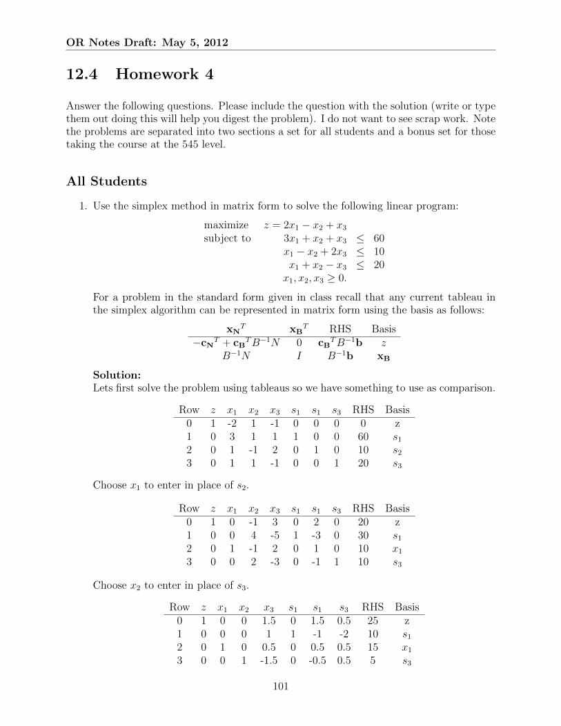
OR Notes Draft: May 5, 2012
12.4 Homework 4
Answer the following questions. Please include the question with the solution (write or typethem out doing this will help you digest the problem). I do not want to see scrap work. Notethe problems are separated into two sections a set for all students and a bonus set for thosetaking the course at the 545 level.
All Students
1. Use the simplex method in matrix form to solve the following linear program:
maximize z = 2x1 − x2 + x3
subject to 3x1 + x2 + x3 ≤ 60x1 − x2 + 2x3 ≤ 10x1 + x2 − x3 ≤ 20x1, x2, x3 ≥ 0.
For a problem in the standard form given in class recall that any current tableau inthe simplex algorithm can be represented in matrix form using the basis as follows:
xNT xB
T RHS Basis−cN
T + cBTB−1N 0 cB
TB−1b zB−1N I B−1b xB
Solution:Lets first solve the problem using tableaus so we have something to use as comparison.
Row z x1 x2 x3 s1 s1 s3 RHS Basis0 1 -2 1 -1 0 0 0 0 z1 0 3 1 1 1 0 0 60 s1
2 0 1 -1 2 0 1 0 10 s2
3 0 1 1 -1 0 0 1 20 s3
Choose x1 to enter in place of s2.
Row z x1 x2 x3 s1 s1 s3 RHS Basis0 1 0 -1 3 0 2 0 20 z1 0 0 4 -5 1 -3 0 30 s1
2 0 1 -1 2 0 1 0 10 x1
3 0 0 2 -3 0 -1 1 10 s3
Choose x2 to enter in place of s3.
Row z x1 x2 x3 s1 s1 s3 RHS Basis0 1 0 0 1.5 0 1.5 0.5 25 z1 0 0 0 1 1 -1 -2 10 s1
2 0 1 0 0.5 0 0.5 0.5 15 x1
3 0 0 1 -1.5 0 -0.5 0.5 5 s3
101

OR Notes Draft: May 5, 2012
Here we have achieved the optimal solution with x1 = 15, x2 = 5, and x3 = 0 theoptimal objective is 25.
For this problem we make the following definitions in order to solve the problem usingthe matrix simplex method:
x =
x1
x2
x3
s1
s2
s3
, c =
2−1
1000
, b =
601020
and
A =
3 1 1 1 0 01 −1 2 0 1 01 1 −1 0 0 1
.
In order to implement the simplex algorithm in matrix format we break the givencoefficient matrix A into to parts: a basic part and a non-basic part. Thus,
A = [N |B]
In matrix form we start by defining xB = (s1 s2 s3)T , and xN = (x1 x2 x3)T we have:
N =
3 1 11 −1 21 1 −1
, B =
1 0 00 1 00 0 1
=⇒ B−1 =
1 0 00 1 00 0 1
.
with
cNT =
(2 −1 1
)cB
T =(
0 0 0)
Evaluating each of the expressions in the tableau we have:
−cNT + cB
TB−1N =(−2 1 −1
)cB
TB−1b =(
0)
B−1b =
601020
B−1N =
3 1 11 −1 21 1 −1
Note that the non-basic variable x1 should be picked to enter the basis. Doing theratio test using the first column of B−1N and the current right hand side vector B−1b:
min
{60
3= 20,
10
1= 10,
20
1= 20
}102

OR Notes Draft: May 5, 2012
and we choose s2 to leave the basis. This leads to the new values for
xB = (s1 x1 s3)T , and xN = (s2 x2 x3)T we have:
N =
0 1 11 −1 20 1 −1
, B =
1 3 00 1 00 1 1
=⇒ B−1 =
1 −3 00 1 00 −1 1
.
with
cNT =
(0 −1 1
)cB
T =(
0 2 0)
Evaluating each of the expressions in the tableau we have:
−cNT + cB
TB−1N =(
2 −1 3)
cBTB−1b =
(20)
B−1b =
301010
B−1N =
−3 4 −51 −1 2−1 2 −3
Note that the non-basic variable x2 should be picked to enter the basis. Doing the ratiotest using the second column of B−1N and the current right hand side vector B−1b:
min
{30
4= 7.5,
10
2= 5
}and we choose s3 to leave the basis. This leads to the new values for
xB = (s1 x1 x2)T , and xN = (s2 s3 x3)T we have:
N =
0 0 11 0 20 1 −1
, B =
1 3 10 1 −10 1 1
=⇒ B−1 =
1 −1 −20 1
212
0 −12
12
.
with
cNT =
(0 0 1
)cB
T =(
0 2 −1)
103

OR Notes Draft: May 5, 2012
Evaluating each of the expressions in the tableau we have:
−cNT + cB
TB−1N =(
32
12
32
)cB
TB−1b =(
25)
B−1b =
10155
B−1N =
−1 −2 112
12
12
−12
12−3
2
We note here that none of the reduced costs given in −cNT + cB
TB−1N are negative, andwe have reached the optimal solution z = 25 when
s1 = 10, x1 = 15, and x2 = 5.
545 Additional Homework
1. The following tableau for a maximization problem was obtained when solving a linearprogram:
Row z x1 x2 x3 x4 x5 x6 RHS Basis0 1 0 a 0 b c 3 d z1 0 0 -2 1 e 0 2 f x3
2 0 1 g 0 -2 0 1 1 x1
3 0 0 0 0 h 1 4 3 x5
Find conditions on the parameters a, b, . . . , h so that the following statements are true.(In the solution parameters that can take on any value will not be mentioned).
(a) The current basis is optimal.Here the current basis is optimal if:
• c := 0 as x5 is basic.
• a and b need to be non-negative making no non-basic variable attractive.
(b) The current basis is the unique optimal basis.
• c := 0 as x5 is basic.
• a and b must be positive to guarantee no alternate optimal solutions.
(c) The current basis is optimal but alternative optimal bases exist.
• c := 0 as x5 is basic.
• Either a and b must be zero with the following sub-cases.
104

OR Notes Draft: May 5, 2012
– If a = 0 then for g > 0 would give an alternate optimal solution. Wheng ≤ 0 the ratio test would not be restrictive and there would be a directionof alternate optimal solutions.
– If b = 0 then for when either e or h or both are positive we would havean alternate optimal solution. If both e and h are negative then ratiotest would not be restrictive and there would be a direction of alternateoptimal solutions.
(d) The problem is unbounded.Assume again that c = 0 as x5 is basic. The problem will be unbounded in twocases:
• a < 0 and g ≤ 0.
• b < 0 and e, h ≤ 0.
In both cases we would have an attractive variable that would enter into the basis,and the ratio test would not have to restrict the value of the decision variables tobe non-negative.
(e) The current solution will improve if x4 is increased. When x4 is entered into thebasis, the change in the objective function is zero.The current solution will improve if x4 is increased means that b will be the mostattractive. We will rig the other parameters such that after entering the objectivefunction does not change.
• c = 0 as x5 is basic.
• b < 0 and a ≥ 0 making x4 attractive.
• e > 0, f = 0 and h > 0. Will assure e wins the Ratio Test, and will have noeffect on the value of d when Row 1 is added to Row 0.
12.5 Homework 5
The following question comes from Nash and Sofer’s text book.
1. The following questions apply to the linear program:
minimize z = −101x1 + 87x2 + 23x3
subject to 6x1 − 13x2 − 3x3 ≤ 11
6x1 + 11x2 + 2x3 ≤ 45
x1 + 5x2 + x3 ≤ 12
with x1, x2, x3 ≥ 0.
with the following optimal basic solution:
Row z x1 x2 x3 s1 s2 s3 RHS Basis0 1 0 0 0 -12 -4 -5 -372 z1 0 1 0 0 1 -2 7 5 x1
2 0 0 1 0 -4 9 -30 1 x2
3 0 0 0 1 19 -43 144 2 x3
105

OR Notes Draft: May 5, 2012
All of the following questions are independent.Before addressing each of the following questions we should note that the problem canbe written in matrix form by defining xB = (x1 x2 x3)T , and xN = (s1 s2 s3)T , withthe optimal basic solution given above represented as:
xNT xB
T RHS Basis−cN
T + cBTB−1N 0 cB
TB−1b zB−1N I B−1b xB
where
B =
6 −13 −36 11 21 5 1
, N =
1 0 00 1 00 0 1
,
b =
114512
, cB =
−1018723
, and cN =
000
.
Note that
B−1b =
512
, and cTBB−1b =
(−372
)It now becomes easy to use sensitivity analysis to answer the following questions.
• What is the solution of the linear program obtained by decreasing the right handside of the second constraint by 15?Here we adjust the value of the original RHS b to the new value:
bnew =
113012
We look to see if the RHS of the LP’s constraints are still feasible:
B−1bnew =
1 −2 7−4 9 −3019 −43 144
113012
=
35−134
647
As the value for x2 = −134 it is no longer a feasible value. We make note thatthe optimality condition is still satisfied. We can do a pivot of the Dual simplexmethod in order to obtain a feasible solution. Here we scan the second row ofB−1N in order to find negative values on which we can pivot. We conduct theratio test by looking at the minimum of the corresponding reduced cost dividedby the possible pivot entry. This gives,
B−1N =
1 −2 7−4 9 −3019 −43 144
1 0 00 1 00 0 1
=
1 −2 7−4 9 −3019 −43 144
, and
106

OR Notes Draft: May 5, 2012
−cNT + cB
TB−1N =(−12 −4 −5
)Ratio Test:
min
{∣∣∣∣−12
−4
∣∣∣∣ = 3,
∣∣∣∣ −5
−30
∣∣∣∣ =1
6,
}this shows that s3 should enter the basis in the place of x2. Doing this updategives:
B =
6 0 −36 0 21 1 1
, and N =
1 0 −130 1 110 0 5
with
B−1bnew =
115
110
0215− 3
101
−15
15
0
113012
=
56156715195
, and cBTB−1bnew =
(−869
3
)and the reduced costs are now:
−cNT + cB
TB−1N =(−34
3−11
2−1
6
)Here we have found a feasible and optimal solution to the updated problem withthe decision variables: x1 = 56
15and x3 = 19
5yielding an objective function value
of z = −8693
.
• By how much can the right hand side of the second constraint increase and de-crease without changing the optimal basis?For this problem we need to consider keeping
B−1b∆b ≥ 0,
where
b∆b =
114512
+
0∆b0
by finding the values of x that satisfy the given inequality. This specifically gives: 1 −2 7−4 9 −3019 −43 144
1145 + ∆b
12
=
11− 2(45 + ∆b) + 7(12)−44 + 9(45 + ∆b)− 30(12)
19(11)− 43(45 + ∆b) + 144(12)
≥ 0
00
Simplifying the three in equalities gives:
∆b ≤ 5
2, ∆b ≥ −1
9, ∆b ≤ 2
43
This shows that the change in the right hand side value of the second constraint∆b must be
−0.111111111 ≈ −1
9≤ ∆b ≤ 2
43≈ 0.0465116
in order for the given basis to remain optimal.
107

OR Notes Draft: May 5, 2012
• What is the solution of the linear program obtained by increasing the coefficientof x1 in the objective by 25?Increasing the coefficient may allow for some other value to be more attractivein the objective function. To see if this has occurred we need to recalculate thevalue of the nonbasic variable reduced costs. After the adjustment
cB =
−768723
, and cN =
000
=⇒ −cNT + cB
TB−1N =(
13 −54 170)
This shows that s3 is now the most attractive to enter into the basis. A pivot ofthe standard simplex method is now done. Here
min
{5
7,
2
144
}gives that x3 should leave the basis so the new basic and nonbasic variable sets arexB = (x1, x2, s3)T and xN = (s1, s2, x3)T . Checking the optimality and feasibilityof this new solution gives:
−cNT + cB
TB−1N =(−679
72−233
72−85
72
)and
B−1b =
11144
13144
0− 1
24124
019144− 43
1441
114512
=
353721712172
as the optimality and feasibility conditions respectively, and the optimal value ofthe objective function is:
cBTB−1b =
11144
13144
0− 1
24124
019144− 43
1441
114512
=(−8977
36
)with x1 = 353
72≈ 4.9072, and x2 = 17
12≈ 1.4167.
• By how much can the objective coefficient of x3 increase and decrease withoutchanging the optimal basis?To solve this we keep N , B, and cN as given initially and consider finding valuesof ∆c that keep
− cNT + cB
TB−1N ≤ 0T (12.5.3)
when the vector
cB =
−10187
23 + ∆c
.
From (12.5.3) we have
−(
0 0 0)+(−101 87 (23+∆c))
1 −2 7−4 9 −3019 −43 144
1 0 00 1 00 0 1
≤ 0
00
108

OR Notes Draft: May 5, 2012
=⇒ (−101 87 (23 + ∆c))
1 −2 7−4 9 −3019 −43 144
≤ 0
00
This gives the following bounds on ∆c:
∆c ≤ 12
19, ∆c ≤ −4
43∆c ≤ 5
144
Thus the coefficient on x3 may vary as follows and the given basis will still beoptimal:
0.09302 ≈ −4
43≤ ∆c ≤ 5
144≈ 0.04372.
• Would the current basis remain optimal if a new variable x4 were added tothe model with objective coefficient c4 = 46 and constraint coefficients A4 =(12,−14, 15)T ?Here we add a new entry in with the non-basic variables, and check the optimalityconditions. Thus,
−cNT + cB
TB−1N =(−209 −12 −4 −5
)where we have use the following values
cN =
46000
, and N =
12 1 0 0−14 0 1 0
15 0 0 1
and we note that the current basis will remain optimal.
545 Additional Homework
These questions are a continuation of the problem listed above (Note they are still indepen-dent questions):
1. Determine the solution of the linear program obtained by adding the constraint
5x1 + 7x2 + 9x3 ≤ 50.
For problems where new constraints are added we can add the as new rows to thegiven optimal tableau. Update the tableau and do needed pivots in order to obtainoptimality. Thus,
Row z x1 x2 x3 s1 s2 s3 s4 RHS Basis0 1 0 0 0 -12 -4 -5 0 -372 z1 0 1 0 0 1 -2 7 0 5 x1
2 0 0 1 0 -4 9 -30 0 1 x2
3 0 0 0 1 19 -43 144 0 2 x3
new 0 5 7 9 0 0 0 1 50 s4
109

OR Notes Draft: May 5, 2012
Updating the tableau to accommodate the new constraint gives:
Row z x1 x2 x3 s1 s2 s3 s4 RHS Basis0 1 0 0 0 -12 -4 -5 0 -372 z1 0 1 0 0 1 -2 7 0 5 x1
2 0 0 1 0 -4 9 -30 0 1 x2
3 0 0 0 1 19 -43 144 0 2 x3
new 0 0 0 0 -148 334 -1121 1 0 s4
Note that adding a new constraint allows us to add an additional variable to theconstraints. Choosing xB = (x1, x2, x3, s4), and xN = (s1, s2, s3) gives:
B =
6 −13 −3 06 11 2 01 5 1 05 7 9 1
=⇒ B−1 =
1 −2 7 0−4 9 −30 019 −43 144 0
−148 334 −1121 1
and
N =
1 0 00 1 00 0 10 0 0
=⇒ −cNT + cB
TB−1N =(−12 −4 −5
)It can be seen from either treatment that the objective function is not changed by theaddition of the new constraint to the problem.
2. Determine the solution of the linear program obtained by adding the constraint
x1 + x2 + x3 ≥ 10.
For this problem we need to note that an excess variable is added to the constraintbefore it is placed in with the other constraints. We have two options to see howthis constraint effects the problem. The easiest is to add the new constraint at thebottom of the given optimal tableau, and then update the tableau as needed to regainan optimal feasible solution.
Row z x1 x2 x3 s1 s2 s3 e1 RHS Basis0 1 0 0 0 -12 -4 -5 0 -372 z1 0 1 0 0 1 -2 7 0 5 x1
2 0 0 1 0 -4 9 -30 0 1 x2
3 0 0 0 1 19 -43 144 0 2 x3
new 0 1 1 1 0 0 0 -1 10 ?
Multiply the new constraint by a ‘-1’ in order to allow e1 to be basic.
Row z x1 x2 x3 s1 s2 s3 e1 RHS Basis0 1 0 0 0 -12 -4 -5 0 -372 z1 0 1 0 0 1 -2 7 0 5 x1
2 0 0 1 0 -4 9 -30 0 1 x2
3 0 0 0 1 19 -43 144 0 2 x3
new 0 -1 -1 -1 0 0 0 1 -10 e1
110
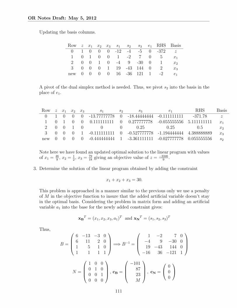
OR Notes Draft: May 5, 2012
Updating the basis columns.
Row z x1 x2 x3 s1 s2 s3 e1 RHS Basis0 1 0 0 0 -12 -4 -5 0 -372 z1 0 1 0 0 1 -2 7 0 5 x1
2 0 0 1 0 -4 9 -30 0 1 x2
3 0 0 0 1 19 -43 144 0 2 x3
new 0 0 0 0 16 -36 121 1 -2 e1
A pivot of the dual simplex method is needed. Thus, we pivot s2 into the basis in theplace of e1.
Row z x1 x2 x3 s1 s2 s3 e1 RHS Basis0 1 0 0 0 -13.77777778 0 -18.44444444 -0.111111111 -371.78 z1 0 1 0 0 0.111111111 0 0.277777778 -0.055555556 5.111111111 x1
2 0 0 1 0 0 0 0.25 0.25 0.5 x2
3 0 0 0 1 -0.111111111 0 -0.527777778 -1.194444444 4.388888889 x3
new 0 0 0 0 -0.444444444 1 -3.361111111 -0.027777778 0.055555556 s2
Note here we have found an updated optimal solution to the linear program with valuesof x1 = 46
9, x2 = 1
2, x3 = 79
18giving an objective value of z = −3346
9.
3. Determine the solution of the linear program obtained by adding the constraint
x1 + x2 + x3 = 30.
This problem is approached in a manner similar to the previous only we use a penaltyof M in the objective function to insure that the added artificial variable doesn’t stayin the optimal basis. Considering the problem in matrix form and adding an artificialvariable a1 into the base for the newly added constraint gives:
xBT = (x1, x2, x3, a1)T and xN
T = (s1, s2, s3)T
Thus,
B =
6 −13 −3 06 11 2 01 5 1 01 1 1 1
=⇒ B−1 =
1 −2 7 0−4 9 −30 019 −43 144 0−16 36 −121 1
N =
1 0 00 1 00 0 10 0 0
, cB =
−101
8723M
, cN =
000
111

OR Notes Draft: May 5, 2012
and using the matrix formulations given we have:
−cNT + cB
TB−1N =(−16M − 12 36M − 4 −121M − 5
)cB
TB−1b =(
22M − 372)
B−1b =
512
22
B−1N =
1 −2 7−4 9 −3019 −43 144−16 36 −121
Note that it is now attractive to have s2 enter the basis. Thus, conducting a pivot ofprimal simplex gives
min
{1
9,22
36
}for the ratio test, and we see that x2 will leave.
xBT = (x1, s2, x3, a1)T and xN
T = (s1, x2, s3)T
Thus,
B =
6 −13 −3 06 11 2 01 5 1 01 1 1 1
=⇒ B−1 =
19
0 13
0−4
91 −10
30
−19
0 23
00 0 −1 1
N =
1 −13 00 11 00 5 10 1 0
, cB =
−101
023M
, cN =
0870
and using the matrix formulations given we have:
−cNT + cB
TB−1N =(−124
9−4M + 4
9−M − 55
3
)cB
TB−1b =(
18M − 33449
)B−1b =
47919
619
18
B−1N =
19
29
13
−49
19−10
3
−19
439
23
0 −4 −1
112

OR Notes Draft: May 5, 2012
We note here that we have reached a point where no variable is attractive to enter intothe basis; however, we still have a basic artificial variable. Thus, the solution to theproblem is not feasible.
113

OR Notes Draft: May 5, 2012
114
Bibliography
[1] H. A. Eiselt and C.-L. Sandblom. Linear programming and its applications. Springer,Berlin, 2007.
[2] Frederick S. Hillier and Gerald J. Lieberman. Introduction to operations research. Holden-Day Inc., Oakland, Calif., third edition, 1980.
[3] D. Luenberger. Linear and nonlinear programming. Addison-Wesley, Reading, Mass.,second edition, 1984.
[4] David G. Luenberger and Yinyu Ye. Linear and nonlinear programming. InternationalSeries in Operations Research & Management Science, 116. Springer, New York, thirdedition, 2008.
[5] S. Nash and A Sofer. Linear and nonlinear programming. McGraw-Hill, New York, 1996.
[6] J. Reeb and S. Leavengood. Using the graphical method to solve linear programs. Ore-gon State University: Extension Service, Performance Excellence in the Wood ProductsIndustry:1–24, 1998.
[7] Hamdy A. Taha. Operations research. An introduction. The Macmillan Co., New York,1971.
[8] Wayne L. Winston. Operations research: applications and algorithms. Duxbury Press,Boston, MA, 1987.
115

Index
complementary slackness, 56
dual simplex method, 58
elementary row operation, 8
sensitivity analysis, 61simplex method, 5strong duality, 50
116