Not quite crisp, not yet fuzzy?

1

Not quite crisp, not yet fuzzy?

Assessing the potentials and pitfalls of multi-value QCA1

Maarten Vink

University of Maastricht / University of Lisbon

[email protected]

Olaf van Vliet

University of Leiden

[email protected]

COMPASSS Working Paper WP 2007-52

(26 November 2007)

Abstract

This paper assesses the strengths and shortcomings of multi-value Qualitative Comparative

Analysis (mvQCA), a comparative technique for small to medium size datasets that has been

integrated in the TOSMANA software developed by Lasse Cronqvist. Its main difference with

Charles Ragin´s ´crisp-set´ QCA (csQCA), which only allows for conditions with 0 or 1 values,

is that the dataset can also contain causal conditions with three or more categories. MvQCA

thus avoids relatively crude dichotomization and arguably better captures the richness of

information of the raw data. Unlike ´fuzzy-set´ QCA (fsQCA), developed by Ragin to go

beyond the classic dichotomous approach, mvQCA is still based on dichotomous outcomes and

applies Boolean minimization principles in a similar way to csQCA. Its major advantage,

according to its proponents, is that it deals better with the classic QCA problem of contradictory

configurations where cases with the same explanatory characteristics display different outcomes

and in principle cannot be taken into account for logical minimization. We discuss the logical

status of mvQCA, its impact on limited diversity, and present a re-analysis of a recent paper to

show how mvQCA uses threshold-setting to solve contradictions.

1 We thank Rapaela Schlicht and Simone Ledermann for their helpful comments and suggestions.

mailto:[email protected]

mailto:[email protected]

2

1. A generalization of crisp-set QCA?

Qualitative Comparative Analysis (QCA), in essence a family of comparative

techniques that aim to explain macro-social phenomena in a parsimonious way while

working with small to medium-sized datasets (5 to 50 cases), is increasingly gaining

ground as a comparative technique that is able to bridge the often lamented qualitative-

quantitative divide in social sciences (Rihoux 2003; Mahony and Goertz 2006). QCA

was originally developed by Charles Ragin (1987) on the basis of Boolean logic, where

both explanatory factors (ćonditions´) and the phenomenon to be explained (óutcome´)

are dichotomized into conditions with 0 and 1 values. This was later termed ćrisp-set´

QCA (csQCA) as dichotomization distinguishes among cases who are either ´fully in´

or ´fully out´ of a particular set (e.g. the set of democratic countries). These distinctions

are wholly qualitative in nature as csQCA only looks at differences in kind, and not at

differences in degree. Later, however, Ragin developed an alternative ´fuzzy-set´

technique (fsQCA) that does not try to force-fit cases into one of only two categories,

but allows the scaling of membership scores in the {0,1} interval. Hence a case can be

attributed a partial or ´fuzzy´ membership score of {0.8} or {0.9} to indicate strong, but

not quite full membership in a set (Ragin 2000).

The availability of software has been an important reason why an increasing number of

people now work with QCA.2 One core intuitive appeal of QCA is its relatively

straightforward analytical framework, which makes it very different from the ´black-

box´ character of most advanced statistical tools. However, the greater the number of

cases and the number of explanatory conditions, the more time-consuming and

particularly the more mistake-prone a manual analysis becomes. Software can facilitate

the construction of truth tables and the production of minimal formulae, and in some

applications also visualize the results. A first version of the QCA software developed by

Charles Ragin with Kriss Drass was made available in 1992 (Drass and Ragin 1992). It

works under DOS and has been improved and updated up to 1998. Subsequently, in

1999 a new fs/QCA version was made available, which works in a Windows

2 The COMPASSS bibliographical database counts around 2000 published and unpublished papers, about

QCA or about comparative configurational methods more generally, with many papers from the last few

years (see http://www.compasss.org).

http://www.compasss.org/

3

environment, and is also continuously updated. This version includes options for both

crisp-set and fuzzy-set analysis (Ragin et al 2006).

Since 2003 an alternative software package is available, called TOSMANA (´Tool for

Small-N Analysis´), which was developed and is continuously updated by Lasse

Cronqvist (2007). There are visual and substantial differences between TOSMANA and

fs/QCA. Visually, TOSMANA is clearly a more user-friendly program, at least in terms

of the whole outlook of the program and the presentation of results. Moreover, with the

addition of a ´Thresholdsetter´ and a Venn-diagram ´Visualizer´, TOSMANA adds two

analytical aids that are much to be welcomed (see also Schneider and Grofman 2006 on

a discussion of presentational forms). Both packages apply different algorithms, but in

principle abide to the same minimization rules. The main substantial difference between

fs/QCA and TOSMANA is that the latter package cannot do fuzzy-set analysis, but

instead includes a novel procedure called ´multi-value´ QCA (mvQCA).

MvQCA allows some explanatory conditions to have more than just two values,

typically three, in order to allow for a more subtle clustering. It can be viewed as a kind

of middle-way between the greater parsimony of csQCA and the greater empirical

richness of fsQCA. It is ńot quite crisp´ because it allows the use of intermediate values

to denote degrees of set-membership, but it is also ńot yet fuzzy´ because the outcome

is always dichotomous. So far, while the TOSMANA program is widely used and

mvQCA is included as one of three established QCA techniques in an important

forthcoming textbook (Rihoux and Ragin 2008), there has been very little debate about

the logical status and the added value of multi-value QCA (but see Schneider and

Wagemann 2007: 262-265 for a brief reflection). Cronqvist argues that mvQCA can be

viewed as a generalization of csQCA (Cronqvist 2004, 2005) and that, particularly for

´genuinely middle-sized´ datasets, mvQCA is often a preferable technique over either

csQCA or fsQCA (Herrmann and Cronqvist 2006). This paper aims to discuss these

claims. After a reflection on the logical status of mvQCA, we raise two issues: how

mvQCA deals with ´limited diversity´ and how it uses thresholds to solve ćontradictory

configurations´. Subsequently, in order to assess whether mvQCA actually is better able

to explain empirical phenomena, we present a re-analysis of a recent application by

Herrmann and Cronqvist (2006). We conclude with an overall evaluation of the

potentials and pitfalls of mvQCA.

4

2. The logical status of mvQCA

QCA has its roots in set theory. Many social scientific statements are of set-theoretic

nature. Imagine a simplistic version of a democratic peace argument: democracies do

not go to war. If a country is a democracy it will not fight a war. Such a statement,

which we know to be factually false, could be phrased in set-theoretic terms: as all

countries in the set of democracies are also in the set of non-warring countries, the set of

democracies is a sub-set of non-warring countries. This argument could be phrased

again in other terms: democracy is a sufficient condition for peace. Of course, such a

statement does not imply that there may not be non-democratic countries that also do

not fight wars. Were such countries to exist, they would not undermine our democratic

peace argument, but merely show that there may be alternative routes to ´peace´, and

that democracy is just one of these. Only if we would argue that non-democracies

always go to war while democracies never go to war, would the existence of a non-

warring non-democracy have undermined our statement. In other words: if democracy

would not only be a sufficient but also necessary condition for non-war (on necessary

and sufficient conditions, see also Goertz 2003, 2006; Goertz and Starr 2003; Mahoney

and Goertz 2006). This statement is however even less plausible than our original

already simplistic thesis and such ´symmetric´ arguments, where the absence and

presence of our phenomenon of interest (peace) are explained by the absence and

presence of the same factor (democracy), are generally rare (Ragin 2006).

Although csQCA and fsQCA require different minimization procedures both are based

on an approach that uses subset relations to find necessary and/or sufficient conditions.

Whereas finding subset relations in a truth table is more straightforward in crisp-set

analysis, in principle fuzzy-set analysis follows the same line of thinking (this holds

even more after the revised version of fuzzy-set analysis presented in Ragin 2008). For

necessary conditions, all cases displaying the outcome should also display the condition

(or the fuzzy-set score for the condition should be equal or higher than the fuzzy-set

score for the outcome). For sufficient conditions, all cases displaying the condition

should also display the outcome (or the fuzzy-set score for the outcome should be equal

or higher than the fuzzy-set score for the condition). One difference between the two is

that fuzzy-set analysis is less hampered by ´deviant´ cases, or errors, as the use of the

notions of consistency and coverage introduces a degree of flexibility (Ragin 2006).

5

The main difference between crisp-set and fuzzy-set analysis, however, is not technical,

but a different approach towards the question whether the most interesting variation in

social reality is only qualitative, and thus about differences in kind, or whether we

should also try to capture differences of degree. These different approaches

subsequently translate in different conceptions of set-membership: whereas in csQCA

set-membership is ćrisp´ as cases are either ín´ {1} or óut´ {0} a set, in fsQCA set-

membership can be partial as cases can be ´more or less´ in {0.8} or out {0.2} a set.

Note, however, that in both approaches set-membership remains limited to the interval

between 0 and 1 and that cases thus can never be more than ´fully´ in or out a set.

Moreover, while fuzzy-set analysis allows for different degrees of set-membership, the

´qualitative threshold´ {0.5} is always the point below which cases are more out than in,

and above which cases are more in than out. This ´middle-value´ reflects the binary

logic of set-theory, and implies that it is an easy step to go back from fuzzy-set scores to

crisp-set scores (this procedure is incorporated in the fs/QCA software).

Multi-value QCA, which can also use intermediate values to denote different degrees of

set-membership, may initially seem a like a crude version of fuzzy-set analysis. In fact,

however, it is explicitly presented as a ´generalization´ of crisp-set QCA (Cronqvist

2004: 3; 2005: 2). The logical status of mvQCA can be better understood by looking at

multi-value logic, which has been developed since the 1930s to cope with the idea that

many propositions are both partially true and partially false. Think of the statement

´John is tall´. If John measures 1m75, we may well say that he is ńot short´, but

probably would not be very confident saying that he is ´tall´. So is John a member of the

set of ´tall people´, or not? Multi-valued logic presents an alternative to classic binary

logic, where items are either members of a given set or not, by incorporating conditions

that consist of more than two categories. Unlike fuzzy logic, however, multi-valued

logic usually does not go beyond three-valued conditions and in any case always has a

strictly finite domain space. In fuzzy-set analysis, which was developed in the early

1970s as an extension of multi-valued logic (Chen and Pham 2001: 57), interval-ratio

conditions can even use the whole {0,1} range to denote degrees of set membership.

This leads to an infinite number of logical combinations, which means that the rows of a

truth-table still indicate the qualitative ´kind´ of membership (in or out) but not the

actual degree of fuzzy-set membership. Because fuzzy-set membership should be seen

in a continuous vector space rather than in a discrete truth table row, x-y plots are a

6

better visual aid in fuzzy-set analysis to represent sub-set relations than Venn diagrams,

which are used in crisp-set analysis (Ragin 2008; Schneider and Wagemann, 2007: 197-

207). The construction of multi-valued truth-tables, on the other hand, is similar to

crisp-set analysis because adding an extra value to a condition does not change the

discrete nature of that condition. Adding an extra value enlarges the number of logically

possible combinations (more on this in the next section), but the number of points in the

domain space remains finite. Boolean algebra can thus be directly applied to multi-

valued logic (Brayton and Khatri 1999: 198).

MvQCA stays very close to csQCA, but uses a different set of values than the classic

Boolean set of {0,1}. Multi-value ´values´ can be either {0, 1, 2}, as is used within

mvQCA, but this could also have been {0, 0.5, 1} or even {-1, 0, 1}. Just as in Boolean

algebra, where the classic values {0} and {1} are mostly a result of convention, these

values only differentiate one qualitative state from another and they do not imply any

pre-defined logical meaning or even ordering (Lablans 2007). In other words, {0} could

mean ´false´, or ´out´, or ´low´, but it could also indicate a state which is simply

qualitatively different from the other two categories, as in the example of race/ethnicity

which may consist of such categories as European American, African American, Native

American, Asian American, and so on (Ragin 2000: 153). These categories are clearly

not ranked in any ordinal sense, which means that any value labeling would be literally

meaningless. There is also no mathematical need to do so as Boolean multiplication and

addition is not arithmetic (Ragin 1987: 91). The three, or more, categories are simply

qualitatively different states and are also viewed as such by the software.

So why do we need mvQCA at all? Cronqvist often mentions the colors of a traffic

light: red, yellow, green. Imagine that a researcher wants to find out whether car

accidents at crossings can be explained by the color of the traffic-light at the moment

when cars cross the traffic-light. As there are three colors, the only way to determine

the effect of each individual color is to create ´dummy conditions´ for each individual

color: one set ´red´, one ´yellow´ and one ´green´ (Cronqvist 2004: 4; 2005: 4). This is

the classic binary way of dealing with multi-value nominal conditions in crisp-set

analysis (Ragin 1987: 86; 2000: 153). Cronqvist rightly argues that this solution leads to

logically impossible combinations, and thus to empty and unnecessary truth-table rows

(e.g. a truth-table row of cases which are both red, yellow and green). His solution is to

7

introduce one new ´multi-value´ condition with three values –red, yellow, green– which

would be more plausible as it excludes logically impossible combinations and more

efficient as it leads to less empty truth-table rows in comparison to adding three

dichotomous conditions. Although this example, as said, is frequently used to show the

added value of mvQCA, there are at least five ways in which it is less appropriate and

convincing than would seem perhaps at first sight.

First, even though a binary solution could lead to logically impossible combinations (the

red, yellow and green traffic-light), this problem is less serious than Cronqvist suggests

as all these impossible combinations can be mapped to the ´don´t care´ set (Brayton and

Khatri 1999: 197). Strictly speaking these don´t care rows in the truth-table are a

reflection of limited diversity, but they have little impact because they can easily be

excluded from the analysis (this option is incorporated in both fs/QCA and

TOSMANA).

Second, the ´problem´ of dummy conditions is also less significant because in the

example of the colors of the traffic light one would not need three, but rather two

dummy conditions. After all, if a color is neither red nor yellow (and scores {0} on both

dummy conditions), it must be green. Even though that would mean that the causal

relevance of ´red´ can only be shown indirectly through the absence of the other two

colors (Schneider and Wagemann, 2007: 263, fn. 88), this is strictly speaking similar to

what would happen in crisp-set analysis with a bi-nominal condition as ´democracy´

(where e.g. authoritarian regimes are treated as non-democracies).

Third, one can go even a step further in the traffic-light example and ask why we would

create a dummy for each of the three colors altogether. Would not a more plausible

strategy be to think about which of the three colors theoretically would have a positive

effect on the outcome? If we think that cases with a positive outcome (cars that crash)

concern cars that crossed the red light, we introduce a set of ´red colors´ to test for this

assumption. Subsequently, if a car crosses the red light, it is in the ´red´ set and is

scored as 1, and cars crossing the traffic-light at either green or yellow are scored as 0.

If, on the other hand, we think that crossing the yellow light would be the most

dangerous (e.g. because cars are likely to speed up just to cross the traffic-light before it

turns red), we define a ´yellow´ set which means that cars crossing the yellow traffic-

8

light are scored 1 and those crossing red and green are scored as 0. If, finally, we

believe that red and yellow are equally dangerous, we define a red-yellow set, and give

a score of 0 only to those cars crossing the green traffic-light. In other words, even when

dealing with multicategory nominal conditions a crisp-set solution is available without

creating dummy conditions for every single category, or even for more than one.

Fourth, the traffic-light example is not very representative in as far as it aims to

legitimize mvQCA by pointing at a problem –dealing with multi-valued nominal

conditions– that seems almost non-existent if one looks at the existing mvQCA

applications. In as far as we can see most, or even all, mvQCA applications so far have

used multi-value conditions with ordered or ranked categories (e.g. low-medium-high),

such as GNP per capita (Cronqvist 2004; Cronqvist and Berg-Schlosser 2007), the

percentage of family-sized landholdings as percentage of the total area of holdings

(Herrmann and Cronqvist 2006) or mortality rates (Cronqvist and Berg-Schlosser 2006).

Apart from the perhaps ill-chosen nature of the traffic-light example, this has important

consequences for the status of mvQCA vis-à-vis the crisp-set and fuzzy-set alternatives.

For example, whereas race or ethnicity is clearly a condition that is difficult to combine

with the potentially continuous fuzzy-set logic, mortality rates would pose no problem

in principle (particularly when trying to explain a continuous outcome as HIV/AIDS

prevalence, see Cronqvist and Berg-Schlosser 2006). In other words, the case for

mvQCA as a distinct approach from fsQCA is less obvious than it may seem. The same

goes, in a different way, for the case against the crisp-set alternative. Whereas for

multichotomous conditions such as race one may still have a case for multi-valued logic

over the alternative of creating crisp-set dummies (but see our hesitations above), with

conditions such as GNP per capita this case is much less obvious. We show this at the

end of the next section and in our re-analysis of Herrmann and Cronqvist (2006).

Fifth, the most important downside of multi-value QCA is arguably that it is very

difficult to understand in set-theoretic terms. With multi-category nominal conditions,

as in the traffic-light example, this is most obvious as the values {0,1,2} do not denote

different forms (either kinds or degrees) of set-membership but simply qualitatively

different states. Every value indicates full set-membership and is, as it were, a ´set´ in

itself while no value can indicate non-set-membership. Multi-valued conditions in a

way should be seen as multiple sets combined in one ´set´. For ordinal or interval three-

9

valued conditions, there is a specific set-theoretic problem with the middle value {1}, as

there is no need in mvQCA to define whether the middle group should be considered as

either ´more or less in´ or ´more or less out´ of the set, or even as ńeither in, nor out´. It

is thus not true that éach multi-value variable can be treated as a dichotomous variable´

(Cronqvist 2004: 3). On the contrary, without specification by the researcher there is no

way to dichotomize a multi-value condition. Note that this is a difference with fuzzy-set

QCA where the value {0.5} always denotes ńeither in, nor out´, and values below this

qualitative anchor can be recoded as {0} and above as {1}. Moreover, as threshold-

setting is a largely inductive process in mvQCA and the researcher is not forced to make

a judgment call about the cases that fall in the medium category, the whole analysis

retains a certain degree of causal ambiguity. This may be particularly problematic when

making simplifying assumptions about logical remainders that fall into this middle

category (see e.g. Ragin and Sonett 2004 on the problem of counterfactuals).

3. Limited diversity and contradictory configurations

While the use of multi-value conditions thus in principle is feasible with the truth-table

approach of crisp-set QCA, particularly when limited to three-valued causal conditions

in combination with binary outcome conditions, the case for mvQCA as a QCA

technique to deal with nominal variables (the traffic-light example) is neither very

relevant nor fully convincing. However, when applied to ordinal or even interval

variables, an additional and potentially important advantage needs to be discussed. This

arguably more significant argument comes down to the claim that crisp-set

dichotomization forces cases into a straightjacket which may not fit the natural

distribution of scores of cases for specific conditions and that therefore the analysis of

causal configurations can be improved by using a categorization which better ´fits´ the

data. In particular, mvQCA is argued to deal better with the classic QCA problems of

´limited diversity´ and ćontradictory configurations´ (Cronqvist 2004, 2005).

´Limited diversity´ is the phenomenon that not all logically possible combinations of

conditions exist in a dataset, or even in reality, which imposes particularly strong

constraints on testing causal arguments in macro-comparative research. Some

combinations are either logically impossible (´pregnant men´ or ‘dictatorial

democracy’) or historically implausible (´black female American presidents´ or ‘African

10

Bismarckian welfare states’). We can therefore never test, for example, whether

Protestantism would have the same effects on socio-economic modernization in

Southern European countries as it had in Northern Europe, simply because

Protestantism was never predominant in Southern Europe. Moreover, it only takes eight

dichotomous conditions to outrun the number of existing countries (28 or 256 logical

combinations). Four dichotomous conditions already leads to thirty-two logical

possibilities, which would require more cases than most middle-sized comparative

studies include. However, researchers may include these so-called ´logical remainders´

(logically possible instances that are not represented by an empirical case in the dataset)

in the minimization process by making so-called ‘simplifying assumptions’. To get the

most simple solutions the software assumes empty rows as having either outcome {0}

or outcome {1}. Researchers can, however, not apply this kind of counterfactual

analysis in a ‘mechanistic fashion’ as strong assumptions are made about causation

(Ragin and Sonnet, 2004: 6). QCA truth-tables make explicit which combinations of

factors are non-existent in the dataset and thus warn against the implicit and unjustified

use of these ´logical remainders´ for causal explanations (Ragin, 1987: 104-113).

´Contradictory configurations´ are empirical cases that share the same explanatory

characteristics (e.g. countries that are rich and democracies) but display differences on

the outcome condition (e.g. most rich and democratic countries have relatively low rates

of gun-related deaths, but some have a high rate). The immediate consequence is that

these cases, which represent a distinct row in the truth-table, cannot be used for logical

minimization, at least not in a crisp-set analysis. One classic strategy to approach this

problem is to reconsider the theoretical framework and to introduce a new explanatory

factor which may distinguish the contradictory cases with a positive outcome from

those with a negative outcome, which solves the contradiction (Ragin 1987: 113;

Rihoux and De Meur 2008). An important downside to introducing new conditions,

however, is that every added explanatory factor exponentially increases the number of

logically possible combinations of conditions (represented in truth-table rows). This, in

turn, implies a greater risk of empty truth-table rows (logical remainders) and

individualizing ´explanations´ (which describe one empirical case).

MvQCA offers an alternative strategy to solve the problem of contradictory rows by not

adding a new condition, but only a new category or value to one or more conditions. If,

11

as a consequence, cases are grouped more ´naturally´, that should imply that the same

´kind of cases´ end up in the same ´kind of group´ which shares the same score on the

outcome condition. Hence the contradiction is solved, without adding a new condition.

Herrmann and Cronqvist (2006: 7) argue that, in terms of limited diversity, the crisp-set

strategy of solving contradiction by adding an extra condition is problematic because

´each added condition leads to an exponential increase in possible causal combinations´.

They argue that mvQCA offers a more attractive alternative, by adding an extra value to

an existing condition instead of adding an extra condition. This improvement needs to

be qualified, however. It is true that adding one extra value for one condition leads to

fewer extra logically possible combinations than would be the result of adding one extra

condition, but this is not the case when adding two extra categories to one existing

condition or one extra category to two existing conditions. After all, truth tables have as

many rows as there are logically possible combinations of values of the causal

conditions (Ragin 1987: 87), and adding an extra value to one causal condition also

increases the number of truth-table rows.

This can be explained further by looking at the formal expressions of the number of

logically possible combinations (truth table rows) for both csQCA and mvQCA. For

csQCA, which only uses dichotomies, the number of logically possible combinations is

equal to 2k, where k stands for the number of dichotomous conditions (Ragin 2000:

127). This means that two conditions lead to four truth-table rows (22), three conditions

to eight rows (23), four conditions to sixteen rows (2

4), etcetera. When, however, one or

more causal conditions are not dichotomous, but have three or more ´values´ or

categories, the number of possible combinations is expressed as follows:

Number of truth table rows (mvQCA) = 2k2

* 3k3

… * nkn

where

k = number of conditions

n = number of categories

This means that, for example, a causal framework with two dichotomous conditions (22)

and one trichotomous condition (31) leads to twelve possible combinations (4*3), a

framework with one dichotomous condition (21) and two trichotomous conditions (3

2)

12

to eighteen combinations (2*9), etcetera. The number of values can be extended

infinitely to conditions with four or more values, although authors who have worked

with mvQCA so far have kept their frameworks limited to trichotomous conditions.

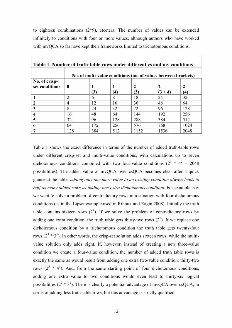
Table 1 shows the exact difference in terms of the number of added truth-table rows

under different crisp-set and multi-value conditions, with calculations up to seven

dichotomous conditions combined with two four-value conditions (27 * 4

2 = 2048

possibilities). The added value of mvQCA over csQCA becomes clear after a quick

glance at the table: adding only one more value to an existing condition always leads to

half as many added rows as adding one extra dichotomous condition. For example, say

we want to solve a problem of contradictory rows in a situation with four dichotomous

conditions (as in the Lipset example used in Rihoux and Ragin 2008). Initially the truth

table contains sixteen rows (24). If we solve the problem of contradictory rows by

adding one extra condition, the truth table gets thirty-two rows (25). If we replace one

dichotomous condition by a trichotomous condition the truth table gets twenty-four

rows (23 * 3

1). In other words, the crisp-set solution adds sixteen rows, while the multi-

value solution only adds eight. If, however, instead of creating a new three-value

condition we create a four-value condition, the number of added truth table rows is

exactly the same as would result from adding one extra two-value condition: thirty-two

rows (23 * 4

1). And, from the same starting point of four dichotomous conditions,

adding one extra value to two conditions would even lead to thirty-six logical

possibilities (22 * 3

2). There is clearly a potential advantage of mvQCA over csQCA, in

terms of adding less truth-table rows, but this advantage is strictly qualified.

Table 1. Number of truth-table rows under different cs and mv conditions

No. of multi-value conditions (no. of values between brackets)

No. of crisp-

set conditions 0

1

(3)

1

(4)

2

(3)

2

(3 + 4)

2

(4)

1 2 6 8 18 24 32

2 4 12 16 36 48 64

3 8 24 32 72 96 128

4 16 48 64 144 192 256

5 32 96 128 288 384 512

6 64 172 256 576 768 1024

7 128 384 512 1152 1536 2048

13

More importantly, do we actually need mvQCA to solve contradictions? The key to

solving contradictions is a re-grouping of cases. Cases can be re-grouped by adding a

new condition to the causal model, which is one classic crisp-set solution (but see

Rihoux and De Meur 2008 for other strategies), or by adding an extra threshold to one

or more of the existing causal condition, which is the multi-value solution. In both

cases, however, adding an extra condition or an extra value, leads to an increasing

number of truth-table rows and thus, possibly, also to more logical remainders. Even

though these can be used for logical minimization, researchers need to be explicit about

this, take care not to make contradictory simplifying assumptions, and arguably also

refrain from making ´difficult counterfactuals´ (Ragin and Sonnet 2004). All other

things being equal, solving contradictions without adding either extra conditions or

extra values would be the most preferable solution.

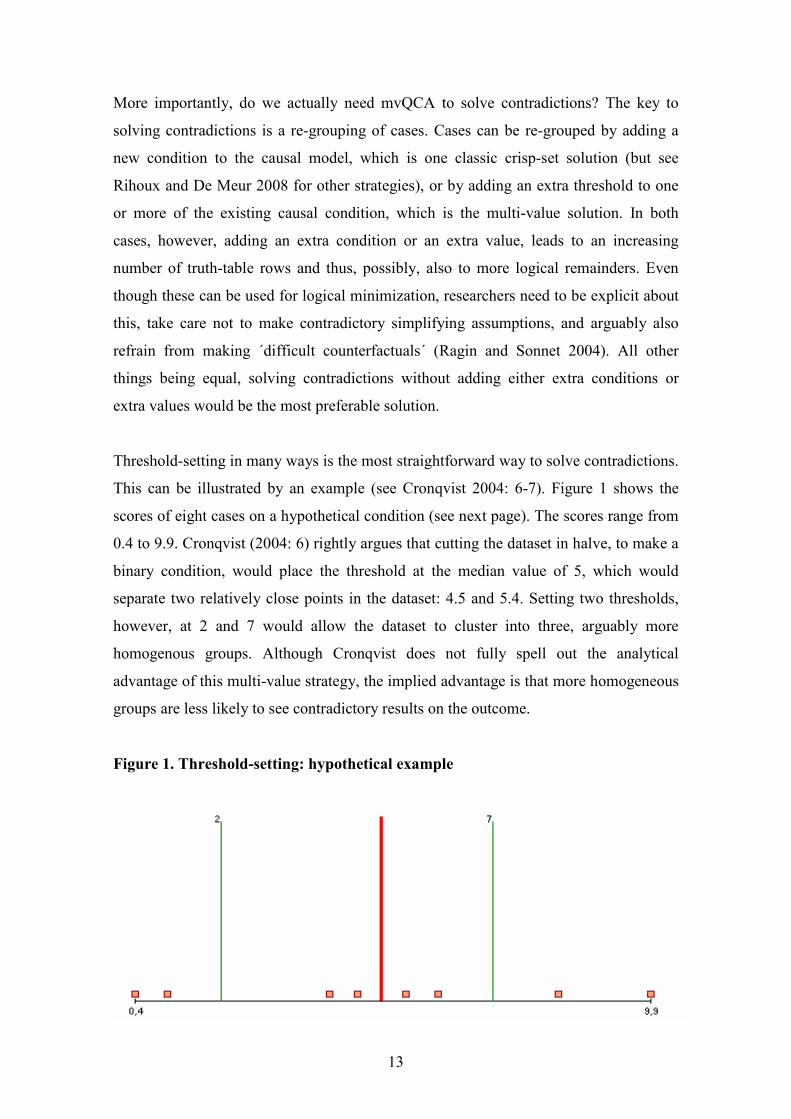
Threshold-setting in many ways is the most straightforward way to solve contradictions.

This can be illustrated by an example (see Cronqvist 2004: 6-7). Figure 1 shows the

scores of eight cases on a hypothetical condition (see next page). The scores range from

0.4 to 9.9. Cronqvist (2004: 6) rightly argues that cutting the dataset in halve, to make a

binary condition, would place the threshold at the median value of 5, which would

separate two relatively close points in the dataset: 4.5 and 5.4. Setting two thresholds,

however, at 2 and 7 would allow the dataset to cluster into three, arguably more

homogenous groups. Although Cronqvist does not fully spell out the analytical

advantage of this multi-value strategy, the implied advantage is that more homogeneous

groups are less likely to see contradictory results on the outcome.

Figure 1. Threshold-setting: hypothetical example

14

What is important is that even though setting the crisp-set threshold at the level of the

median value may have some intuitive plausibility, at least more than the alternative of

using the arithmetic average, there is no reason why in this example a value of 5 should

be the ´best´ crisp-set threshold. Keep in mind the classic guideline that ´substantive and

theoretical criteria´ should be used for the dichotomization of interval-scale conditions

(Ragin 1987: 86-87). Given the relative close distance between the four middle-scores

displayed in Figure 1, it may be more sensible to either include or exclude this group as

a whole in the set, by setting the threshold either below the lowest or above the highest

value of the four. This may lead to an unequal number of cases that are either in or out

(6 vs. 2), but at least it does not split up the relatively homogeneous middle group. And

it can be done without introducing an extra middle-value. The importance of threshold-

setting will be further illustrated by the following re-analysis.

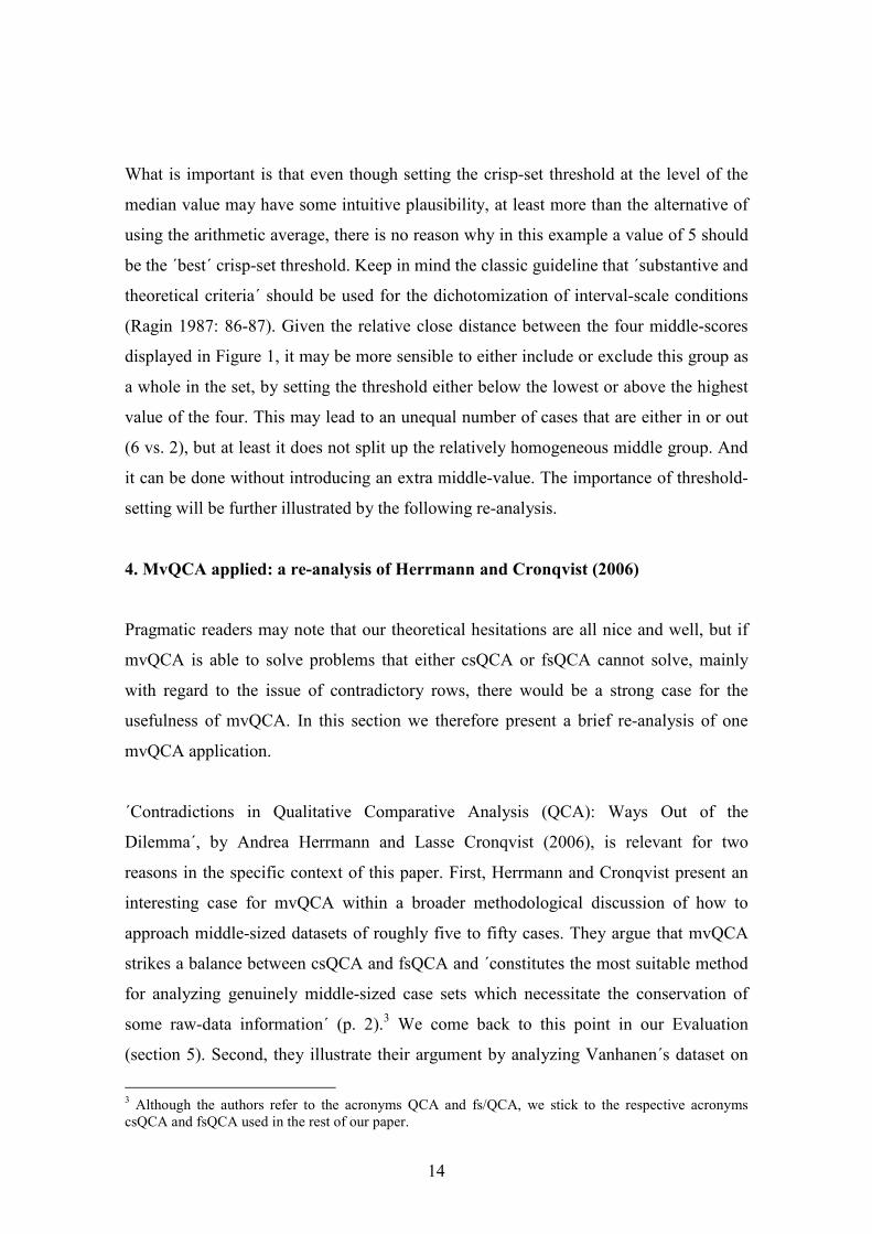
4. MvQCA applied: a re-analysis of Herrmann and Cronqvist (2006)

Pragmatic readers may note that our theoretical hesitations are all nice and well, but if

mvQCA is able to solve problems that either csQCA or fsQCA cannot solve, mainly

with regard to the issue of contradictory rows, there would be a strong case for the

usefulness of mvQCA. In this section we therefore present a brief re-analysis of one

mvQCA application.

´Contradictions in Qualitative Comparative Analysis (QCA): Ways Out of the

Dilemma´, by Andrea Herrmann and Lasse Cronqvist (2006), is relevant for two

reasons in the specific context of this paper. First, Herrmann and Cronqvist present an

interesting case for mvQCA within a broader methodological discussion of how to

approach middle-sized datasets of roughly five to fifty cases. They argue that mvQCA

strikes a balance between csQCA and fsQCA and ´constitutes the most suitable method

for analyzing genuinely middle-sized case sets which necessitate the conservation of

some raw-data information´ (p. 2).3 We come back to this point in our Evaluation

(section 5). Second, they illustrate their argument by analyzing Vanhanen´s dataset on

3 Although the authors refer to the acronyms QCA and fs/QCA, we stick to the respective acronyms

csQCA and fsQCA used in the rest of our paper.

15

the emergence of democratic regimes and present a multi-value analysis against the

crisp-set alternative. Herrmann and Cronqvist also present a fuzzy-set analysis of the

same dataset, which we leave aside in this paper. We do so for two reasons. First, it is

based on an older, by now somewhat outdated version of fsQCA (see Ragin 2008 for a

more recent approach). Second, fuzzy-set analysis is highly problematic –if not

meaningless– when using a dichotomized outcome, as Herrmann and Cronqvist do. We

analyze the raw dataset on the causes of democratic breakdown and survival of eighteen

countries in the interwar period as it is included in Herrmann and Cronqvist´s paper (p.

4). It should be stressed that our sole interest is methodological and that we do not aim

to present a novel theoretical argument. We have used TOSMANA Version 1.3 to

analyze the data (available since 27 June 2007).

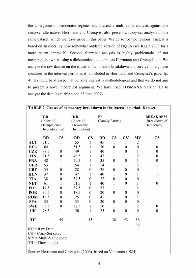
TABLE 2. Causes of democracy breakdown in the interwar period: Dataset

IOD

(Index of

Occupational

Diversification)

IKD

(Index of

Knowledge

Distribution)

FF

(Family Farms)

BREAKDEM

(Breakdown of

Democracy)

RD CS RD CS RD CS CS´ MV CS

AUT 51,5 1 55 1 45 1 1 2 1

BEL 64 1 51,5 1 30 0 0 0 0

CZE 38,5 0 49 1 40 1 0 1 0

FIN 21,5 0 46,5 1 47 1 1 2 0

FRA 48 1 50,5 1 35 0 0 1 0

GER 53 1 54 1 54 1 1 2 1

GRE 34 0 28 0 28 0 0 0 1

HUN 37 0 47 1 40 1 0 1 1

ITA 38 0 39,5 0 22 0 0 0 1

NET 61 1 51,5 1 40 1 0 1 0

POL 17,5 0 37,5 0 53 1 1 2 1

POR 30,5 0 18,5 0 20 0 0 0 1

ROM 16,5 0 25 0 41 1 0 1 1

SPA 35 0 33 0 20 0 0 0 1

SWE 39,5 0 52,5 1 50 1 1 2 0

UK 78,5 1 50 1 25 0 0 0 0

TH

45

45

38

43

32/

43

RD = Raw Data

CS = Crisp-Set score

MV = Multi-Value score

TH = Threshold(s)

Source: Herrmann and Cronqvist (2006), based on Vanhanen (1984).

16

Table 2 presents the raw dataset used by Herrmann and Cronqvist in their analysis of

breakdown of democracy in the interwar period. In line with an earlier study from Berg-

Schlosser and De Meur (1994) they focus on sixteen countries. The outcome condition

´Breakdown of Democracy´ (which we label BREAKDEM) is already presented in a

dichotomized way, with {0} indicating democracy survival and {1} democracy

breakdown. There are three causal conditions: Index of Occupational Diversification

(IOD), which is an arithmetic mean of urban population and non-agricultural population

in a country; Index of Knowledge Distribution (IKD), which combines measures of

literacy and university education; and Family Farms (FF), which indicates the

percentage of family-sized landholding as a percentage of the total area of holdings.

Next to the raw scores for each of the sixteen countries on these three conditions, Table

2 also presents the initial crisp-set dichotomization of these scores. In order to

determine the cut-off points, Herrmann and Cronqvist make use of the cluster-analysis

function in the TOSMANA threshold-setter which calculates how for each of the three

conditions the distribution of scores arithmetically cluster into two groups. This implies

a threshold of 45 for both IOD and IKD and a threshold of 38 for FF. Although there is

a strong intuitive case for cluster-analysis as it looks for a ´natural gap´ in the raw

dataset, and is also less arbitrary than using the arithmetic mean, the ´textbook´

approach would be to use ´substantive and theoretical criteria´ (Ragin 1987: 87).

From here it is an easy step to convert the dataset into a truth-table, which in this case

contains eight rows with all logically possible combinations of causal conditions. A

quick glance at the first row of Table 3 shows that there are two rows with positive

outcomes, one with a negative outcome, two with contradictory outcomes, and three

empty rows. As discussed in the previous section, contradictory truth-table rows are a

classic problem for QCA, because cases with similar causal characteristics but different

outcomes cannot be used for Boolean minimization, in principle (but see Ragin 1987:

116-118). Empty rows in principle also cannot be used, but researchers can invoke these

´logical remainders´ as hypothetical cases and allow the software to use them for

minimization. For the sake of brevity Herrmann and Cronqvist only minimize the truth-

table for the positive outcome and thus only look at the causal factors for the breakdown

of democracy, and not for those that may explain the survival of democracy.

17

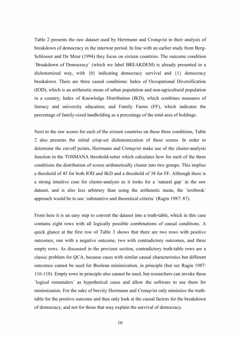
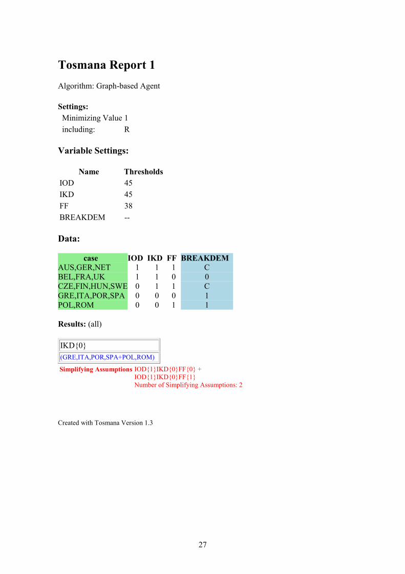
This leads to the following equation, when minimizing for the outcome value {1}

(breakdown of democracy), excluding the contradictory rows, and including logical

remainders (R):

IKD{0} → BREAKDEM{1} (TOSMANA Report 1)

In other words, democracy broke down during the interwar period in countries with an

unequal knowledge distribution. When we go back to Table 3, we see indeed that in

every row with an IKD score of 0 where empirical cases are present (the first two rows),

the BREAKDEM score is {1}. This means that an unequal knowledge distribution is a

sufficient condition for democracy breakdown, as the set of countries with unequal

knowledge distribution is a subset of the countries with democracy breakdown.4

Although this solution is very parsimonious, an important downside is that it covers

only six of the nine countries with a positive outcome, and thus has a coverage of 0,67.5

The solution does not apply to the three ´positive´ cases of Hungary, Austria and

Germany that are part of contradictory rows, which were excluded from the Boolean

minimization. In fact, all three countries have a relatively equal knowledge distribution

4 Contrary, however, to the interpretation from Herrmann and Cronqvist (p. 6), unequal knowledge

distribution is not a necessary condition for democracy breakdown, as becomes clear from the

dichotomized dataset in Table 2: democracy broke down in Austria, Germany and Hungary despite their

relatively equal knowledge distribution. 5 Herrmann and Cronqvist (p. 7) state that 9 out of 16 countries are part of non-contradictory rows and

that the coverage is thus 56%. It should be noted, however, that solution coverage is calculated as ´the

number of cases following a specific path to the outcome divided by the total number of instances of the

outcome´ (Ragin 2006: 299). Hence the coverage is 67% (6 divided by 9).

Table 3. Causes of democracy breakdown: Truth-Table (csQCA)

IOD IKD FF

BREAKDEM Cases

0 0 0 1 POR, GRE, SPA, ITA

0 0 1 1 ROM, POL

0 1 0 – –

0 1 1 C FIN, CZE, SWE (0)

HUN (1)

1 0 0 – –

1 0 1 – –

1 1 0 0 FRA, BEL, UK

1 1 1 C NET (0)

AUT, GER (1)

18

(an IKD score of {1}) and thus suggest that there is an alternative path which also leads

to the outcome. There are a number of ways to proceed from here in order to obtain a

solution with a greater empirical coverage (ideally, of course, explaining all cases with

positive outcomes). One classic solution is to introduce a new causal condition which

may, as it were, ´split´ the contradictory cases from each other (Ragin 1987: 113). We

discussed the implications of this solution on limited diversity in the previous section

(see also a useful discussion of different strategies to deal with contradictions in Rihoux

and De Meur, 2008). Here we focus on the mvQCA solution.

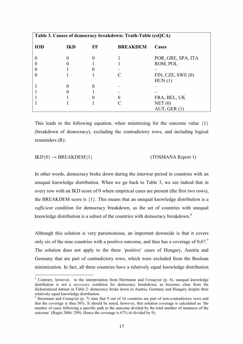
Figure 2. Family farm index (FF): distribution of raw data and multiple thresholds

Figure 2 shows a graphical display of the distribution of cases on the Family Farms

condition, made with the very useful threshold-setting function in the TOSMANA

program. It shows that the scores range from 20% (Portugal and Spain) to 54%

(Germany). The median value is 40. In the initial csQCA analysis, Herrmann and

Cronqvist applied a single threshold of 38% to divide the dataset into countries with low

(0) and high (1) levels of family-sized landholding as a percentage of total area of

holdings (see the middle threshold in Figure 2). Since mvQCA allows the use of

multiple thresholds, however, they apply an ´average linkage method´ (p. 12) which

shows that ´the sixteen cases form roughly three clusters´ (p. 13).6 Accordingly, they

transform the original raw data on the FF condition into a three-point scale {0, 1, 2} by

setting two thresholds at 32 and 43 (see Figure 2 and also the MV column in Table 2 for

6 For the IOD and IKD conditions they find that ´cases are distributed fairly evenly´ (p. 12) on the

original dichotomous scale.

19

the multi-value score of each country). The result is that the truth-table is expanded

from eight to twelve rows (22 * 3

1) and that Austria and Germany, with high FF scores

of respectively 45 and 54 are split from the Netherlands, with a ´medium´ score of 40.

This solves one of the two contradictions as the first two are ´breakdown´ countries,

whereas the latter is a democratic survivor. Finland (47) and Sweden (50) are split from

Czechoslovakia and Hungary (both 40), but as the latter two score different on

BREAKDEM, this still constitutes one remaining contradictory row.

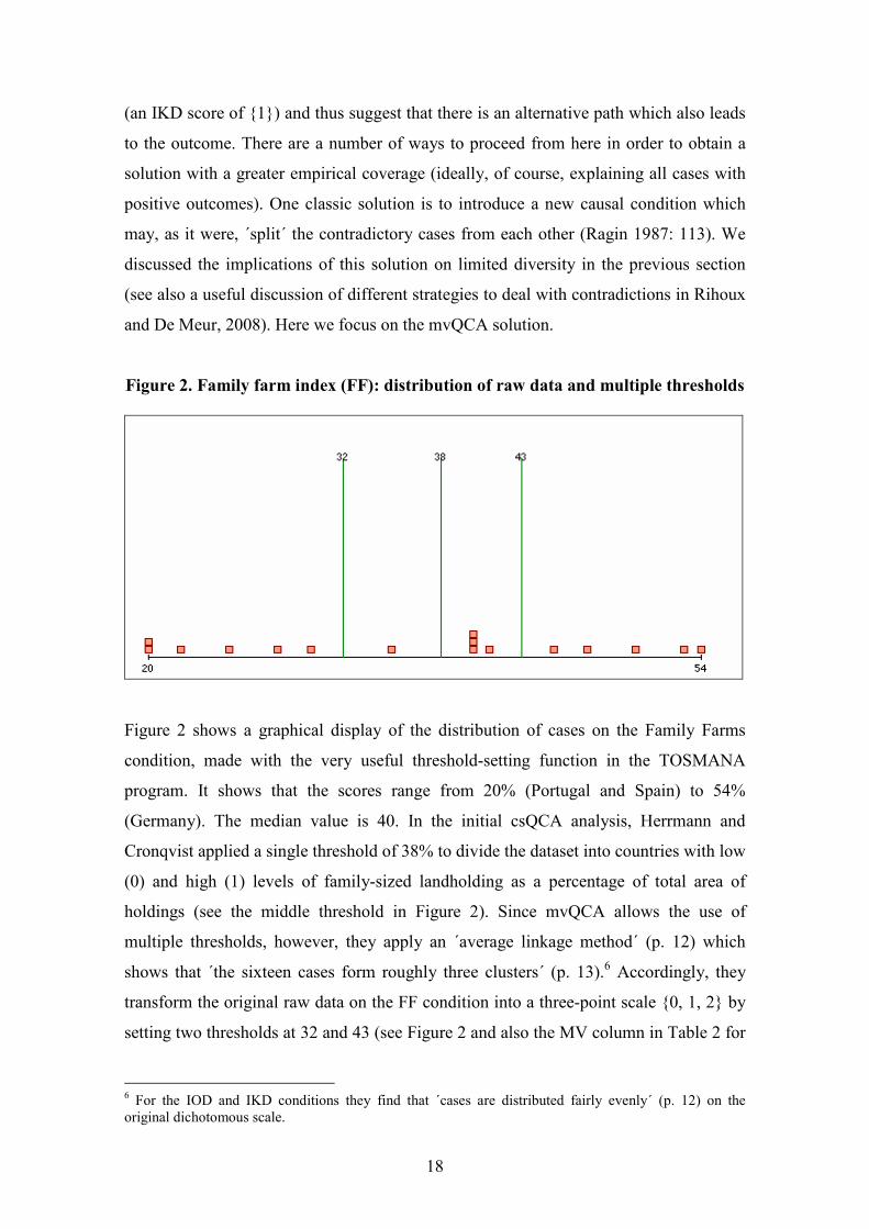
Figure 3. Causes of democracy breakdown: mvQCA ‘Venn’ diagram

↓ 2. IKD

↓ 2. IKD

002

POL

012

FIN, SWE

102

112

AUT, GER

001

ROM

011

CZE

HUN

101

111

FRA, NET

000

POR, GRE,

SPA, ITA

010

100

110

BEL, UK

↑ 3.FF

→ 1. IOD

0 1 C R

Figure 3 shows a visual representation of the new truth-table, which results from

combining two dichotomous causal conditions (IOD and IKD) with one trichotomous

condition (FF). Note that this is an ´unpolished´ diagram that we tentatively designed

ourselves as there currently is no Visualizer available yet in the TOSMANA program

for mvQCA analyses. It keeps the same idea as the Venn diagram for ´crisp-set only´

data, with every field representing a truth-table row, and the color indicating whether a

logical combination of conditions leads to democratic survival (0), to democratic

breakdown (1), to both (C), or whether there is no empirical case representing this

combination (R). The diagram should be read as follows: the right half of the diagram

20

represents fields with score IOD{1}, whereas the second and fourth ´columns´ represent

fields with IKD{1}. The bottom row is for fields with FF{0}, the middle-one for FF{1},

and the top one for FF{2}. Numbers in the top-left of each field indicate the logical

combination of respective IOD, IKD and FF scores. Figure 3 shows that there is now

only one contradictory field, but also that the number of logical remainders (empty

fields) increased from three to four (see also the truth-table in TOSMANA Report 2).

Moreover, whereas there was previously no truth-table row which covered only one

empirical instance, there are now two such ´individual rows´ (for Romania and Poland).

Minimizing for the outcome, including the remainders, and excluding the

contradictions, leads to the following equation:

IKD{0} + IOD{1}*FF{2} → BREAKDEM{1} (TOSMANA Report 2)

In other words, apart from the path indicated by the first column of Figure 3 (unequal

knowledge distribution –note the ´simplifying assumption´ that hypothetical cases that

would fall in the now empty third column would also lead to breakdown), we also have

a path explaining/describing the democracy breakdown in Austria and Germany: a high

level of occupational diversification combined with a high share of family-owned farms.

So does this mean that –in this illustration– mvQCA really does lead to a better analysis

than csQCA? Yes and no. Yes, because even if the solution may be less parsimonious,

this is clearly an advantage as the more complex solution increases the empirical

coverage to 89% (from 67%). Only one positive case, Hungary, is not covered by this

solution but that was also not the case under the original csQCA analysis.

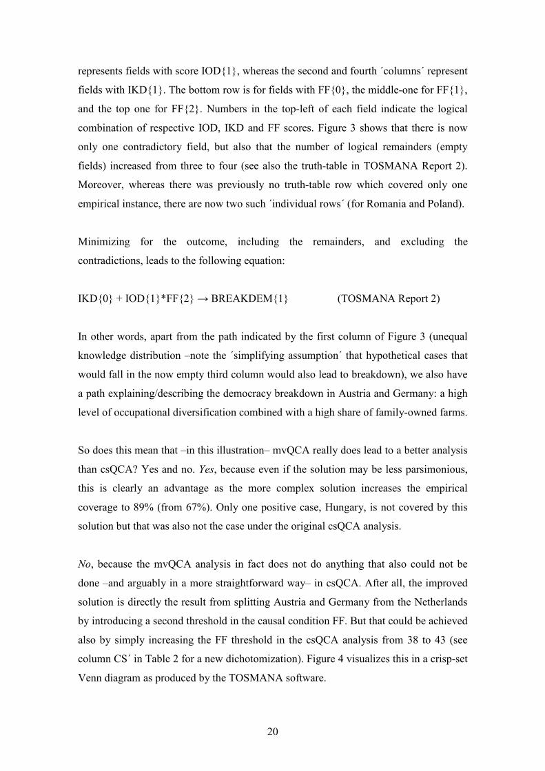
No, because the mvQCA analysis in fact does not do anything that also could not be

done –and arguably in a more straightforward way– in csQCA. After all, the improved

solution is directly the result from splitting Austria and Germany from the Netherlands

by introducing a second threshold in the causal condition FF. But that could be achieved

also by simply increasing the FF threshold in the csQCA analysis from 38 to 43 (see

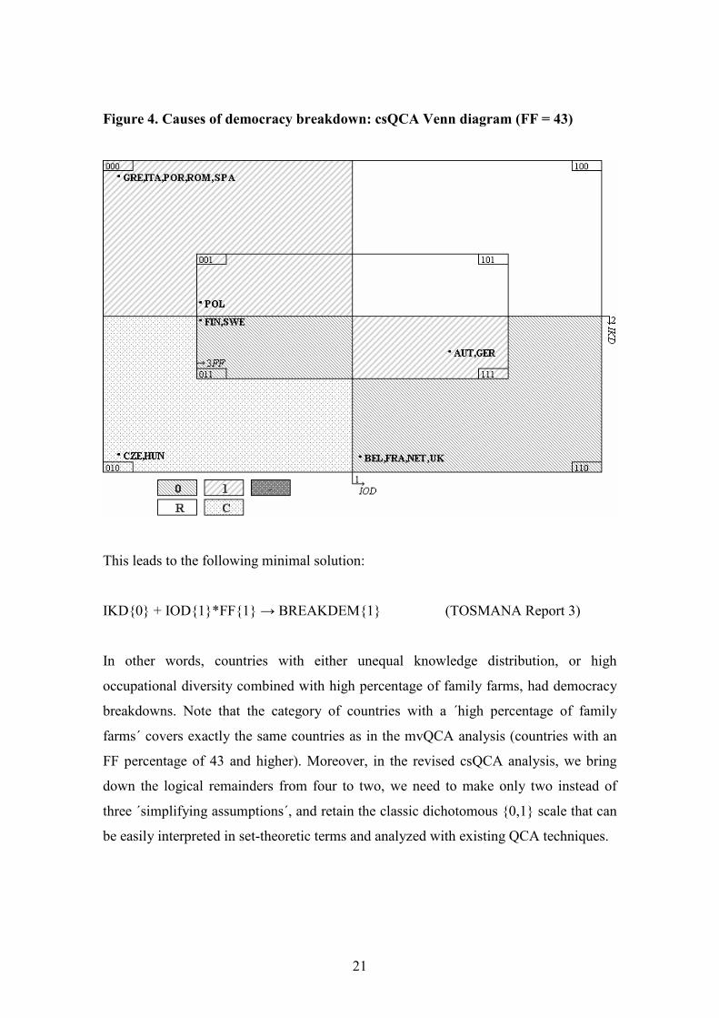
column CS´ in Table 2 for a new dichotomization). Figure 4 visualizes this in a crisp-set

Venn diagram as produced by the TOSMANA software.

21

Figure 4. Causes of democracy breakdown: csQCA Venn diagram (FF = 43)

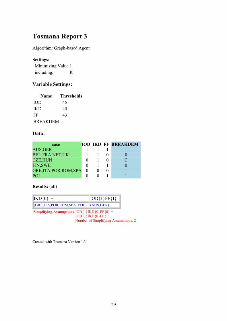
This leads to the following minimal solution:

IKD{0} + IOD{1}*FF{1} → BREAKDEM{1} (TOSMANA Report 3)

In other words, countries with either unequal knowledge distribution, or high

occupational diversity combined with high percentage of family farms, had democracy

breakdowns. Note that the category of countries with a ´high percentage of family

farms´ covers exactly the same countries as in the mvQCA analysis (countries with an

FF percentage of 43 and higher). Moreover, in the revised csQCA analysis, we bring

down the logical remainders from four to two, we need to make only two instead of

three ´simplifying assumptions´, and retain the classic dichotomous {0,1} scale that can

be easily interpreted in set-theoretic terms and analyzed with existing QCA techniques.

22

5. Evaluation

There should be no doubt that the introduction and continuous development of the

software package TOSMANA has significantly contributed to a growing popularity of

QCA as a non-probabilistic comparative method for small to medium sized datasets.

TOSMANA is freely available, easy to use and with the Visualizer and Tresholdsetter

includes two very useful new analytical tools that represent a welcome addition to

already existing packages. In this paper we have reflected on the key methodological

innovation of the TOSMANA program, which is the possibility to do an analysis that is

in many ways similar to crisp-set QCA, but allows for the use of multiple thresholds in

one or more of the causal conditions. Although it is very clear that this methodological

innovation responds to some real problematic issues that QCA researchers invariably

have to deal with, particularly concerning dichotomization, threshold-setting, limited

diversity and contradictory configurations, we are not fully convinced about the solution

offered by multi-value QCA. Our concerns partly result from the fact that so far there

have been only a few mvQCA applications and this means that it simply may be too

early to let the jury out on the question of the potentials and pitfalls of mvQCA. Partly,

however, our hesitations also result from the fact that in introducing mvQCA relatively

much attention has been given to explaining technical procedures such as notation and

minimization, to the new tools incorporated in TOSMANA, and to some illustrations,

while relatively little is said about the logical status of mvQCA and its relation to the –

certainly more established– crisp-set and fuzzy-set alternatives. We hope this paper

contributes to such a more elaborated and more fundamental discussion of mvQCA.

We conclude here by raising three issues that in our view would be central to such a

broader discussion on the potentials and pitfalls of mvQCA: its set-theoretic nature, how

it deals with limited diversity, and the role of threshold-setting. First, as to its set-

theoretical nature, multi-value conditions in a way incorporate multiple sets in one set.

While this may have technical advantages, in terms of limited diversity, the set-theoretic

interpretation of these conditions is unclear. In particular with regard to the middle

values of ordinal or interval multi-value conditions, such as GNP per capita, it is often

unclear whether these are ín´ or óut´ the set, or ńeither in, nor out´. Why bother? One

could argue that introducing a new intermediate category allows us to modify

theoretical expectations, as in the case of Cronqvist and Berg-Schlosser´s (2008) re-

23

analysis of Lipset socio-economic theory of democracy. And one may have good

theoretical reasons to expect a specific causal relevance of an intermediate category,

possibly in combination with other causal conditions. But as most mvQCA analyses use

a form of cluster analysis to decide on the number and the level of thresholds, the

creation of new intermediate categories is a purely inductive affair, which obviously

may be problematic when drawing general conclusions on the basis of only a very small

number of cases. Simplifying complexity is clearly the fundamental goal of comparative

research, but leaving aside the strictly theoretically guided core of the QCA approach

does pose strong limits on the meaningfulness of data reduction. Since theorizing in

both crisp-set and fuzzy-set QCA is in principle of set-theoretic nature the question of

the set-theoretic nature of multi-value QCA is not one that can easily be discarded.

Second, as to limited diversity, a main advantage of mvQCA over csQCA would be that

it deals better with the problem of ‘contradictory configurations’, because introducing

one extra category leads to half as many added truth-table rows in comparison to adding

one new causal condition. This clearly has an advantage in terms of dealing with limited

diversity although, as we showed on the basis of a formula that determines the number

of truth-table rows in mvQCA, this advantage is strictly qualified. Adding two

categories to one condition increases the number of logical combinations to the same

extent as adding one causal condition, while adding one category to two conditions

leads to half as many added truth-table rows.

Third, as to threshold-setting, our re-analysis of Herrmann and Cronqvist (2006)

demonstrates that while multi-value QCA may be one way to solve contradictory

configurations, an equal solution may well be achieved by changing the threshold in

crisp-set analysis to either the lower or upper multi-value thresholds. Such a crisp-set

solution may be preferable for two reasons at least. It would be better in terms of limited

diversity since no truth-table rows are added at all. And, although changing threshold

levels inductively to achieve a minimal solution which covers more empirical cases may

obviously be criticized for the same reasons as stated above, it solves the problem of the

theoretical status of an intermediate category. In other words, changing the threshold

level as such does not influence the expected causal impact of a condition.

24

So is mvQCA indeed more eligible for genuine middle-sized datasets? Hermann and

Cronqvist (2006: 3) argue that ´the likelihood of contradictions increases with the

number of cases’. Therefore, csQCA should be used for small middle-sized datasets,

mvQCA for medium middle-sized datasets and fsQCA for large middle-sized datasets.

We hesitate to go along with such a generalizing argument. One objection concerns the

fundamental difference between csQCA and mvQCA, on the one hand, and fsQCA on

the other. Whereas the crisp-set and multi-value alternatives work with a dichotomized

outcome, fuzzy-set analysis aims to use degrees of variation on the causal configuration

to explain degrees of variation on the outcome. Some outcomes, such as democratic

breakdown, simply cannot be operationalized (easily) in a way other than in

dichotomous terms, which means that fuzzy-set analysis is no realistic alternative.

With regard to choosing between crisp-set and multi-value analysis, we see no reason

why contradictions should be related to the size of the dataset per se, and thus why that

should be a reason to decide between the two. Rather, in as far as we see a case for

multi-value QCA, this is related to the nature of the causal conditions. Despite the

frequently cited example of the three colors of the traffic-light we have not yet seen

mvQCA being applied to a multichotomous nominal causal condition. The case for

mvQCA seems strongest to us, therefore, when it is related to a specific theoretical

expectation of causal relevance of an intermediate category within a condition that is

based on either ordinal or interval-scale data. In such an instance a crisp-set alternative

through changing threshold-levels may not be easily available, or not at all, and multi-

value QCA could well provide a useful solution.

25

Bibliography

Berg-Schlosser, D. and G. de Meur (1994) Conditions of Democracy in Interwar

Europe: A Boolean Test of Major Hypotheses. Comparative Political Studies

26(3) 253-279.

Brayton, R.K. and S.P. Khatri (1999) Multi-valued Logic Synthesis. 12th International

Conference on VLSI Design – VLSI for Information Appliance, pp. 196-205.

Chen, G. and T.T. Pham (2001) Introduction to Fuzzy Sets, Fuzzy Logic and Fuzzy

Control Systems. Boca Raton etc.: CRC Press.

Cronqvist, L. (2004) Presentation of TOSMANA: Adding Multi-Value Variables and

Visual Aids to QCA. COMPASSS Working Papers, 2004-20.

– (2005) Introduction to Multi-Value Qualitative Comparative Analysis

(MVQCA). COMPASSS Didactical Papers, 2005-4.

– (2007) Tosmana: Tool for Small-N Analysis (Version 1.3). Marburg. Available

at: www.tosmana.org.

Cronqvist, L. and D. Berg-Schlosser (2006) Determining the Conditions of HIV/AIDS

Prevalence in Sub-Saharan Africa. Employing New Tools of Macro-Qualitative

Analysis. In B. Rihoux and H. Grimm, eds, Innovative Comparative Methods

for Policy Analysis. New York: Springer, pp. 145-66.

– (2008) Multi-value QCA (mvQCA). In Rihoux/Ragin, forthcoming (Chapter 4).

Drass, K.A. and C.C. Ragin (1992). Qualitative Comparative Analysis 3.0. Evanston,

Illinois: Institute for Policy Research, Northwestern University.

Goertz, G. (2003) Cause, Correlation, and Necessary Conditions. In: G. Goertz and H.

Starr (eds.) Necessary Conditions: Theory, Methodology and Applications. New

York: Rowman and Littlefield Publishers Inc, pp. 47-64.

- (2006) Assessing the Trivialness, Relevance, and Relative Importance of

Necessary or Sufficient Conditions in Social Science. Studies in Comparative

International Development, 41(2), pp. 88-109.

Goertz, G. and H. Starr (2003) Introduction: Necessary Condition Logics, Research

Design, and Theory. In: G. Goertz and H. Starr (eds.) Necessary Conditions:

Theory, Methodology and Applications. New York: Rowman and Littlefield

Publishers Inc, pp. 1-23.

http://www.tosmana.org/

26

Herrmann, A. and L. Cronqvist (2006) Contradictions in Qualitative Comparative

Analysis (QCA): Ways Out of the Dilemma. EUI Working Papers, SPS No.

2006/06.

Lablans, P. (2007) Multi-valued Logic, available at www.multivaluelogic.com.

Mahoney, J. and G. Goertz (2006) A Tale of Two Cultures: Contrasting Quantitative

and Qualitative Research. Political Analysis, 14(3), pp. 227-249.

Ragin, C.C. (1987) The Comparative Method: Moving Beyond Qualitative and

Quantitative Strategies. Berkeley: University of California Press.

– (2000) Fuzzy-Set Social Science. Chicago: University of Chicago Press.

– (2006) Set Relations in Social Research: Evaluating Their Consistency and

Coverage. Political Analysis, 14, 291-310.

– (2008). Qualitative Comparative Analysis Using Fuzzy Sets (fsQCA). In

Rihoux/Ragin, forthcoming (Chapter 5).

Ragin, C.C., K.A. Drass and S. Davey (2006). Fuzzy-Set/Qualitative Comparative

Analysis 2.0. Tucson, Arizona: Department of Sociology, University of Arizona.

Ragin, C.C. and J. Sonnett (2004) Between Complexity and Parsimony: Limited

Diversity, Counterfactual Cases, and Comparative Analysis. COMPASSS

Working Papers, 2004-23.

Rihoux, B. (2003) Bridging the Gap between Qualitative and Quantitative Worlds? A

Retrospective and Prospective View on Qualitative Comparative Analysis. Field

Methods, 15(4) 351-365.

Rihoux, B. and G. de Meur (2008) Qualitative Comparative Analysis using Boolean

Sets (csQCA). In Rihoux/Ragin, forthcoming (Chapter 3).

Rihoux, B. and C. Ragin, eds (2008) Configurational Comparative Analysis. Thousand

Oaks, CA and London: Sage Publications, forthcoming.

Schneider, C.Q. and B. Grofman (2006) It might look like a regression equation…but

it´s not! An intuitive approach to the presentation of QCA and fs/QCA results.

COMPASSS Working Papers, 2006-39.

Schneider, C.Q. and C. Wagemann (2007) Qualitative Comparative Analysis (QCA)

und Fuzzy Sets. Ein Lehrbuch für Anwender und jene, die es werden wollen.

Opladen: Barbara Budrich.

http://www.multivaluelogic.com/

27

Tosmana Report 1

Algorithm: Graph-based Agent

Settings:

Minimizing Value 1

including: R

Variable Settings:

Name Thresholds

IOD 45

IKD 45

FF 38

BREAKDEM --

Data:

case IOD IKD FF BREAKDEM

AUS,GER,NET 1 1 1 C

BEL,FRA,UK 1 1 0 0

CZE,FIN,HUN,SWE 0 1 1 C

GRE,ITA,POR,SPA 0 0 0 1

POL,ROM 0 0 1 1

Results: (all)

IKD{0}

(GRE,ITA,POR,SPA+POL,ROM)

Simplifying Assumptions IOD{1}IKD{0}FF{0} +

IOD{1}IKD{0}FF{1}

Number of Simplifying Assumptions: 2

Created with Tosmana Version 1.3

28

Tosmana Report 2


Settings:

Minimizing Value 1

including: R

Variable Settings:

Name Thresholds

IOD 45

IKD 45

FF 32; 43

BREAKDEM --

Data:

Case IOD IKD FF BREAKDEM

AUS,GER 1 1 2 1

BEL,UK 1 1 0 0

CZE,HUN 0 1 1 C

FIN,SWE 0 1 2 0

FRA,NET 1 1 1 0

GRE,ITA,POR,SPA 0 0 0 1

POL 0 0 2 1

ROM 0 0 1 1

Results: (all)

IKD{0} + IOD{1}FF{2}

(GRE,ITA,POR,SPA+POL+ROM) (AUS,GER)


IOD{1}IKD{0}FF{1} +

IOD{1}IKD{0}FF{2}



29

Tosmana Report 3


Settings:

Minimizing Value 1

including: R

Variable Settings:

Name Thresholds

IOD 45

IKD 45

FF 43

BREAKDEM --

Data:

case IOD IKD FF BREAKDEM

AUS,GER 1 1 1 1

BEL,FRA,NET,UK 1 1 0 0

CZE,HUN 0 1 0 C

FIN,SWE 0 1 1 0

GRE,ITA,POR,ROM,SPA 0 0 0 1

POL 0 0 1 1

Results: (all)

IKD{0} + IOD{1}FF{1}

(GRE,ITA,POR,ROM,SPA+POL) (AUS,GER)


IOD{1}IKD{0}FF{1}



Not quite crisp, not yet fuzzy?

Documents

Transcript of Not quite crisp, not yet fuzzy?