NOT ALL RIVALS LOOK ALIKE: ESTIMATING AN EQUILIBRIUM MODEL ...leinav/pubs/EI2010.pdf · NOT ALL...

NOT ALL RIVALS LOOK ALIKE: ESTIMATING AN EQUILIBRIUMMODEL OF THE RELEASE DATE TIMING GAME

LIRAN EINAV∗

I develop a new empirical model for discrete games and apply it to study the releasedate timing game played by distributors of movies. The results suggest that releasedates of movies are too clustered around big holiday weekends and that box office rev-enues would increase if distributors shifted some holiday releases by one or two weeks.The proposed game structure could be applied more broadly to situations where compe-tition is on dimensions other than price. It relies on sequential moves with asymmetricinformation, making the model particularly attractive for studying (common) situationswhere player asymmetries are important. (JEL C13, C51, L13, L15, L82)

. . .a very serious game of strategy is atwork–a cross between chess and chicken–which studio distribution chiefs play yearround, but with increasing intensity duringthe summer and holiday release period.(New York Times, December 6, 1999)

Hubris. Hubris. If you only think aboutyour own business, you think, “I’ve gota good story department, I’ve got a goodmarketing department, we’re going to goout and do this.” And you don’t think thateverybody else is thinking the same way.In a given weekend in a year you’ll havefive movies open, and there’s certainlynot enough people to go around. (JoeRoth, chairman of Walt Disney Studios,

*This paper partially originates from chapter 1 of my2002 Harvard University dissertation, and I am particularlygrateful to Ariel Pakes for his guidance and support in theearly stages of this paper. I thank three anonymous refereesfor many useful suggestions, and Susan Athey, Pat Bajari,Lanier Benkard, Tim Bresnahan, Peter Davis, Mike Mazzeo,Aviv Nevo, Peter Reiss, Katja Seim, and seminar participantsat the Society of Economic Dynamics 2003 annual meetingin Paris, the Econometric Society 2004 Winter meeting inSan Diego, UW Madison, and the University of Tokyo foruseful comments on earlier drafts. I thank Oren Rigbi forsuperb research assistance, Jeff Blake (Sony Pictures), RonKastner (Goldheart Pictures), and Terry Moriarty (HoytzCinemas) for insightful conversations, and ACNielsen EDIand Exhibitor Relations Inc. for helping me obtain importantportions of the data. I acknowledge financial support fromthe National Science Foundation and the Stanford Institutefor Economic Policy Research.Einav: Associate Professor of Economics, Stanford Uni-

versity, 579 Serra Mall, Stanford, CA 94305-6072;and Research Associate, National Bureau of EconomicResearch, 1050 Massachusetts Avenue, Cambridge, MA02138. Phone 650-723-3704. Fax 650-725-5702,E-mail [email protected].

answering a question about the largenumber of major movies opening withindays of each other; Los Angeles Times,December 31, 1996)

I. INTRODUCTION

The number of Americans who go to themovies varies dramatically over the course ofthe year, and sometimes more than doubleswithin a period of two weeks. At the same time,the first week accounts for almost 40% of thebox office revenues of the average movie. Thecombination of these two facts makes the tim-ing of launching a new movie a major focusof attention for distributors of movies. Withvirtually no subsequent price competition, themovie’s release date is one of the main short-run vehicles by which studios compete with eachother.

In this paper, I develop and estimate a modelof discrete games, which allows me to analyzethis release date timing game. Most empiricalindustry studies focus on price and quantitycompetition, taking other product characteris-tics as given; in many industries, however,prices play a very small role, and competitionis channeled through other product attributes.The entertainment industry is a prime example;competition among movies, television programs,or Broadway shows is on nonmonetary productattributes, such as content, advertising, and time.Therefore, understanding competition in suchindustries requires a model that endogenizessome of these product attributes, especially thosethat can be changed in the short run. This paperprovides a framework in which release decisions

369

Economic Inquiry doi:10.1111/j.1465-7295.2009.00239.x(ISSN 0095-2583) Online Early publication September 28, 2009Vol. 48, No. 2, April 2010, 369–390 © 2009 Western Economic Association International

370 ECONOMIC INQUIRY

can be endogenized and nonprice competitioncan be analyzed.

The absence of price competition is usefulbecause it allows the focus of the analysis tobe on the timing dimension without relyingon assumptions about the nature of the postre-lease price competition.1 Together with the fre-quent timing decisions associated with differentmovies, this makes the motion picture industryquite attractive for empirical analysis of the tim-ing game. This industry, however, is not the onlyexample in which timing decisions play a cen-tral role. Similar timing considerations are alsoimportant in the release decisions of books, com-pact disks, and other new products, as well as inthe scheduling decisions of major events, televi-sion programs, flight schedules, and promotionalsales.2

When taking on a new project, distributors ofmovies typically plan for a Friday release, whichfalls within a relatively short window of timecarefully chosen to match the type of the movie.This makes the choice of the release date a verydiscrete one. The exact Friday within the sea-son is generally determined by a strategic timinggame played among distributors. Before eachrelease season, distributors scramble to releasetheir movies on big holiday weekends, whendemand is high. When doing so, each distributortries to release on the attractive holiday weekendand at the same time to deter competitors fromdoing the same. The extent to which distribu-tors are successful in doing so largely dependson the quality of the movies at their disposal,and on the way they can compete with moviesreleased by other studios. Thus, modeling thistiming game must account for the asymmetriesamong movies, and for the variation in theseasymmetries across release seasons.

Specifically, I develop and estimate a sequen-tial-move game with private information; Iassume that the observed release date decisionsare the equilibrium outcome of such a game. Theempirical analysis relies on data from the U.S.

1. The fact that ticket prices hardly vary across seasonsand movies is taken as given throughout this paper. This isan interesting puzzle, which is discussed in more detail inOrbach and Einav (2007).

2. There are only a few papers that analyze competitionin time. They mostly use reduced-form statistics to assess theequilibrium outcome (Borenstein and Netz 1999; Chisholm1999; Corts 2001; Simonsohn 2008). Goettler and Shachar(2001) construct a strategic scheduling game between tele-vision networks, but do not use it for estimation. Sweeting(2008), who models the timing of radio advertising, is anotable exception.

motion picture industry between 1985 and 1999.I take the season in which a movie is releasedas given, and focus the analysis on the strategicdecision of the specific release date within theseason. To specify payoffs, and in particular toassess the heterogeneous substitution effect indemand between movies, I rely on the estimatesof the demand for movies obtained in a compan-ion paper (Einav 2007). In that paper, I modeleddemand for movies as a function of movie qual-ity, decay in the demand for a movie, and sea-sonal underlying demand for movies. The mainfocus of the analysis in the current study ison evaluating the extent to which distributorsof movies over- or underestimate this underly-ing demand vis-a-vis the substitution effect fromcompeting movies. I find that the release patternimplies that underlying demand for movies ismuch more seasonal than is estimated by thedemand system. That is, the results suggest thatthe release dates of movies are too clusteredon holiday weekends and that distributors couldincrease theatrical revenues by shifting holidayrelease dates by one or two weeks. Differentpossible explanations, such as uncertainty andconservatism, are discussed.

Beyond this specific application, the gamestructure I develop is an important contributionof this paper because it is likely applicable moregenerally. The model builds on ideas from theexisting literature on discrete games, but com-bines these ideas together in a new way, therebyproviding certain attractive properties.3 Themodel is a sequential-move game with asym-metric information. Under certain restrictions onthe private information, one can construct a rel-atively simple pseudo-backward induction algo-rithm to solve for the unique perfect Bayesianequilibrium of the game. For any payoff struc-ture, the sequential structure of the game leadsto a unique probability distribution over allpossible outcomes, thus allowing for a sim-ple maximum likelihood estimation. The privateinformation assumption facilitates evaluation ofthe likelihood function by avoiding the difficul-ties (due to complex regions of integration) thatwould arise with complete information.

An attractive property of the proposed modelis its ability to accommodate an unrestrictedpayoff structure. In particular, the model and its

3. See Section II for more details. See also Reiss(1996), Einav and Nevo (2006), and Draganska et al. (2008)for related reviews and discussions of existing models ofdiscrete games.

EINAV: ESTIMATING THE RELEASE DATE TIMING GAME 371

estimation could accommodate player identitiesand asymmetries in substitution patterns. Sym-metry assumptions, which are crucial for manyexisting empirical models of discrete games, arenot necessary. Such symmetry restrictions oftenseem implausible; in a wide range of industries,decision makers care not about the number ofcompetitors they face but also about competitoridentities. All else equal, a software developer ismore likely to enter a market in which anothersmall software company operates rather than amarket in which Microsoft participates. Simi-larly, a movie distributor would rather releasehis movie during the same week as a low-budget movie release than during the same weekas the Star Wars release. In accordance withthe above observations, studying differentiatedproduct markets and the varying degrees of sub-stitution among products has proven importantin demand estimation.4 The model I proposeallows for the incorporation of players’ identitiesinto models of discrete games and could facil-itate research that combines entry and locationgames with empirical demand models; thus far,these two strands of the literature have evolvedquite independently of each other.

The rest of the paper is organized as fol-lows. Section II presents the model, its prop-erties, and its estimation; it also describes itsrelationship to the existing literature of discretegames and illustrates the differences. Section IIIdescribes the industry and the data, and SectionIV presents the empirical specification and theresults. Section V concludes.

II. THE MODEL

A. The empirical model

Let the set of players in market m be i =1, 2, . . . , Nm and the discrete (finite) actionspace for player i be Am

i . Given the actionsof all players (for simplicity of notation, them subscripts are suppressed), a ∈ A1 × A2 ×· · · × AN , payoffs for player i are given by

πi (a; X, β, η) = πi (a; X, β) + εiai

,(1)

where β is a vector of parameters and εiai

is an i.i.d (across actions and players) drawfrom a type I extreme value distribution with

4. See, among many others, Berry, Levinsohn, and Pakes(1995) and Nevo (2001).

a precision parameter η.5 The vector of εiai

’sis assumed to be private information of playeri. The private information can be thought ofas nonstrategic considerations that may makea certain player more likely to choose a cer-tain action, regardless of the actions of the otherplayers. It could also be thought of as optimiza-tion errors. The magnitude of the estimated ηprovides an indication for the explanatory powerof the model. This is because the variance ofthe unexplained portion of the payoffs, εi

ai, is

decreasing in η, thus η provides a measure ofthe explanatory power of the deterministic partof the payoffs.6 The higher η is the more wecan explain the observed decisions by the esti-mated payoffs rather than by the random error.An insignificant estimate of η implies that themodel for the payoffs has no statistically signif-icant explanatory power.7

This specification leads to simple logit prob-abilities. Conditional on the other players’ deci-sions, a−i , movie i chooses action ai with thefollowing probability:

Pr(ai |a−i ) = (exp(ηπi (a; X, β)))

/

⎛⎝ ∑

a′i∈Ai

exp(ηπi (a′i , a−i; X, β))

⎞⎠ .(2)

The game is played sequentially with eachplayer moving exactly once according to a pre-specified order, which is known to the playersbut may be unknown to the econometrician. Thesolution concept is a perfect Bayesian equilib-rium. Note that the payoffs of each player idepend only on the action taken by the otherplayers, but not on the realizations of theirεjaj

’s (j �= i). Therefore, each player’s strategydepends only on the actions of players whomoved previously, but not on their exact draws

5. This distribution has a cdf F(x) = exp(− exp(−ηx)),mean γ/η (where γ = 0.577 is the Euler’s constant), andvariance π2/6η2. As η goes to 0, the variance goes toinfinity, and as η goes to infinity, the variance goes to 0.

6. To empirically identify η, one must pin down the levelof π through any other assumption. For example, if π = Xβ,it is easy to see that η cannot be separately identified fromβ. In this paper, η is identified because external data is usedto estimate π and pin down its level. More generally, doingso requires some external information that would pin downthe level of one of the other parameters of the model.

7. McKelvey and Palfrey (1998) provide the moregeneral properties of such games, and use it to analyzeexperimental data. This literature uses the term quantalresponse equilibria to describe such games.


of ε′s. This assumption greatly simplifies equi-librium analysis because it implies that from theplayer’s perspective, opponent types are irrele-vant when opponent actions are known. Con-sequently, given the prespecified order of play,the game can be solved backwards in a simpleway.

In what follows, I outline the simple algo-rithm that is used to solve the model. In therest of the paper, I refer to this algorithm aspseudo-backward induction. Given N players,let the order of play be given by a permutationo ∈ PN , such that o(m) = j implies that playerj is the mth player to move. Let prev(j) = {k :o−1(k) < o−1(j)} denote the set of players whoplay before player j. I solve the game backwards.The last player to move, o(N), conditions on theother players’ decisions, a−o(N). Therefore, wecan use Equation (2) to see that ao(N) is chosenwith probability

Pr(ao(N)|a−o(N))

= (exp(ηπo(N)(ao(N), a−o(N); β)))

/

⎛⎜⎝ ∑

a′o(N)

∈Ao(N)

exp(ηπo(N)(a′o(N), a−o(N); β))

⎞⎟⎠ .

(3)

Going backwards, we can update the contin-uation values for all other players by integratingout over player o(N)’s decision probabilities,namely,

πN−1i (a−o(N); β) =

∑ao(N)∈Ao(N)

Pr(ao(N)|a−o(N))

πi (ao(N), a−o(N); β) ∀i ∈ prev(o(N)),(4)

and

π(N−1)i (a−o(N); β, η) = π

(N−1)i (a−o(N); β)

+ εiai

∀i ∈ prev(o(N)).(5)

The key is that the εiai

’s are invariant toa−i , they depend only on ai , so they can betaken out of the sum. These modified payoffswould directly enter the decision of playero(N − 1). They are also updated for the restof the players because we use these modifiedpayoffs below as part of the iterative procedure.In particular, we can use Equation (2) again, butwith respect to the modified payoffs, which aregiven by Equation (4). This procedure can be

done iteratively up to the player who moves first,with each iteration being the following:

Pr(aj |aprev(j)) = (exp(ηπo−1(j)

j (aj |aprev(j)))

/

⎛⎜⎝ ∑

a′j ∈Aj

exp(ηπo−1(j)

j (a′j |ap(j))

⎞⎟⎠,(6)

and

π(o−1(j)−1)

i (aprev(j); β) =∑

aj ∈As

Pr(aj |aprev(j))

π(o−1(j))

i (aj , aprev(j); β) ∀i ∈ prev(j).(7)

Thus, in the end of the procedure we obtaina probabilistic equilibrium play for each player,and hence a strictly positive probability measureover each potential outcome of the game. Inparticular, given an order o, the likelihood ofobserving an outcome a is given by

Pr(a|o) =N∏

j=1

Pr(aj |aprev(j), o).(8)

Given a probability measure over all possi-ble permutations (orders of play), the uncondi-tional likelihood of observing an outcome a isgiven by

f (a) =∑o∈PN

Pr(o) Pr(a|o)

=∑o∈PN

⎡⎣Pr(o)

N∏j=1

Pr(aj |aprev(j), o)

⎤⎦ .(9)

If a natural order of play exists and isobserved, one can use this order and think abouto as being observable. Alternatively, one canassume a uniform distribution over all permuta-tions, i.e., Pr(o) = 1/N !∀o ∈ PN . Finally, whenthe data are rich enough or when there areenough restrictions on the payoff structure, onecan estimate the probabilities of different per-mutations. Although this is not implemented inthe application below, a simple yet general wayto specify the probability measure over the orderpermutations is to assign a commitment measurefor each player, given by μj = Wjδ + ζj , whereζj is distributed i.i.d extreme value, Wj is a vec-tor of observed characteristics of player j whichaffect his commitment power, and δ is a vectorof parameters that can be estimated. The order


of moves is then dictated by the commitmentmeasure μj . This implies that the probability ofan order o is given by

Pr(o) =N∏

j=1

(exp(Wjδ))

/ ∑k /∈ prev(o(j))

exp(Wkδ).

(10)

Given M distinct and independent marketsand a specification for πi (a; X, β), the modelcan be estimated using maximum likelihood.

Finally, it is important to note what wouldbe altered in the model if we considered a per-fect information game, that is, a game of thesame structure in which all ε

jaj

’s are commonknowledge. The key difference, for the econo-metrician, is that the observed decision of, say,the player who moves last provides informationabout that player’s ε

jaj

’s. In the perfect infor-mation case, unlike in the derivation above, theother players know these ε

jaj

’s and hence suchinformation must be taken into account by theeconometrician when assigning probabilities tothe other players’ decisions at earlier points ofthe game. Thus, these decisions would have tobe analyzed in light of a truncated extreme valuedistribution, for which we do not have closed-form solutions. To address this in a useful way,we will need to employ simulation estimators,which will solve for the subgame perfect equi-librium for each set of simulated vectors ofεjaj

’s.8 This complication is the reason why theimperfect information case is computationallymore attractive.

B. Relationship to the Literature

Existence and uniqueness are typically thetwo properties of equilibrium we analyze. Empir-ically, we generally assume that the data aregenerated by an equilibrium behavior, thuseliminating any existence problem. Multiplic-ity, however, remains a major issue. In orderto understand the estimation problems associ-ated with multiplicity of equilibria, let us denotethe empirical model by y(Xi, ε, β) ⊂ Y , that is,a mapping from the model primitives, namely,observables X, unobservables ε, and parametersβ, into the model predicted outcome y(Xi, ε, β),which is a subset of all potential outcomes Y .

8. The appendix of Berry (1992) conceptually describessuch a simulation estimator. With player asymmetries, how-ever, the procedure described there would be computation-ally more intensive.

If y(Xi, ε, β) is a singleton for all Xi’s, β’s,and ε’s (i.e., equilibrium is always unique)then estimation is straightforward: one can pro-ceed with, say, maximum likelihood estimation,with the likelihood of the observed outcome,yi , given by Pr[ε ∈ {ε|yi = y(X, ε, β)}|X, β]. If,however, y(Xi, ε, β) is nonunique then such alikelihood-based estimation procedure cannot becarried out unless we extend the model to havean additional assumption about the probabil-ity measure over the set of possible outcomes,y(Xi, ε, β). Several comments are in place: (1)in general, theory tells us nothing about theseequilibrium selection probabilities; (2) to bespecified correctly, one has to account for allpossible equilibria, for any given (Xi, ε, β); (3)sometimes we may tell a story why one equi-librium is more likely than another, and thiscould be thought of as an extension of the model,which essentially provides uniqueness.

An approach taken by several authors (Berry1992; Bresnahan and Reiss 1990) and morerecently generalized by Davis (2006b) is to setup a model that does not provide uniqueness,but provides the econometrician with a coarserpartition of the empirical model, which satis-fies uniqueness. For example, in the context ofentry models, these authors show that while,given (Xi, ε, β), the model may have multi-plicity of equilibria, all such equilibria share acommon feature, which is the number of enter-ing firms. Thus, the econometrician can condi-tion on the number of entering firms, but noton their identities, and then apply likelihood-based (or other) estimation techniques. This isa coarser partition of Y in the sense that dif-ferent observations are treated the same. Whilethis approach has proven useful, it has two mainlimitations. First, the approach is not efficient inthe sense that it treats different observables inthe same way and hence does not use all theinformation provided by the data.9 Second, amore important limitation is that strong sym-metry assumptions must be imposed to get aunique prediction in models with more than twoplayers. For example, in entry models, firms’payoffs are assumed to be invariant to permuta-tions of the entry decisions made by their oppo-nents. These assumptions seem quite unrealisticfor a wide set of applications in which entrantsare not drawn at random but are endogenously

9. Indeed, Tamer (2003) proposes a more efficient esti-mator, which exploits the additional information providedby the data.


drawn from a well-defined population of het-erogeneous firms. Therefore, for many researchquestions, these models may prove unsatisfac-tory and may alter the economic implicationsof the results. Mazzeo (2002) relaxes this sym-metry assumption by introducing different typesof products, and conditioning the analysis on thenumber of entering firms of each type. The mainrestriction still remains: all potential entrants areex-ante identical, and profits of a player areinvariant to a permutation of his opponents’ typechoices. Moreover, extending Mazzeo’s modelto more than two or three types is computation-ally infeasible. Thus, the main two limitationsremain largely unaddressed.

Two recent alternative approaches to dealwith multiple equilibria have been developed.First, several papers (Andrews, Berry, and Jia2007; Beresteanu, Molchanov, and Molinari2008; Ciliberto and Tamer 2008) show that inthe presence of multiplicity of equilibria, onecan place bounds on the parameters of interestrather than obtain point estimates for them.The potential of these methods has yet tobe fully realized, especially when there existsimportant variation in observable characteris-tics across observations. A second approach(Aguirregabiria and Mira 2007; Bajari, Benkard,and Levin 2007; Pakes, Ostrovsky, and Berry2007) uses a two-step estimation procedureto get around the multiplicity problem. Thisapproach assumes that the game has a reducedform, thereby avoiding the multiplicity prob-lem. It relies heavily on accurate (nonparamet-ric, ideally) estimation of the policy functions,which are then used to back out the structuralparameters. While useful in many settings, thisapproach requires either large data sets or asmall set of state variables. Many of the typicaldata sets and applications in industrial organiza-tion (for which the current paper is an example)do not satisfy either of these requirements.

Finally, a somewhat more structural approachis to change the structure of the game in sucha way that equilibrium would be unique.10

Bresnahan and Reiss (1990) and Berry (1992)suggest ways to do this by imposing a sequen-tial structure on the game, which yields agenerically unique subgame perfect equilibrium.

10. Within this class, I also consider imposing a pre-defined probability distribution over the different equilibria,as in, for example, Bajari, Hong, and Ryan (2008). We canjust think of an additional latent variable (the outcome ofthe “public randomization device”), conditional on whichequilibrium is unique.

This full information version, however, becomescomputationally unattractive as we relax sym-metry assumptions and increase the dimension-ality of the game. Seim (2006) enriches the gamestructure by moving to games with asymmet-ric information. This makes the strategy of eachplayer simpler from the econometrician’s pointof view because it now depends only on thefirm-specific unobserved variables rather than onthe whole set of unobservables in the market.Indeed, Seim (2006) is able to find a uniqueBayesian Nash equilibrium and use it for esti-mation. Several limitations remain. First andforemost, the equilibria in such games are notnecessarily unique.11 Second, the search for theequilibrium strategies must involve an intensivenumerical search for a fixed point, thus makingcomputational complexity increase quite rapidlywith the dimension of the problem. Third, just asin Mazzeo (2002), the same symmetry assump-tions discussed above are still present: all oppo-nents are ex-ante identical.

The model developed in the previous sectionis therefore in the spirit of Seim (2006), but witha sequential structure, as in certain specifica-tions of Bresnahan and Reiss (1990) and Berry(1992). The (standard) assumptions on the pri-vate information structure guarantee uniquenessof equilibrium and imply that the equilibriumcan be found using a pseudo-backward inductionalgorithm, thus alleviating some of the compu-tational burden present in other models. There-fore, it incorporates different existing ideas intoa game structure that guarantees uniqueness, isnot restricted by symmetry assumptions, andis computationally attractive. In entry games,for example, such structure should be particu-larly attractive for situations in which additionalinformation on postentry values is available(e.g., Berry and Waldfogel 1999, Orhun 2005,Ellickson and Misra 2007, or Watson, 2009).Such information would typically make sym-metry assumptions internally inconsistent, and itwould provide valuable insight on the structureof postentry values, which can be easily incor-porated into the game structure just outlined.

11. Seim (2006) numerically shows that there is a uniquesymmetric equilibrium for her particular model and data.More generally, however, there are no assumptions aboutthe model that can guarantee uniqueness. Moreover, oncerivals are allowed to be asymmetric, we would not be able tofocus on symmetric equilibria, thereby the scope of findingmultiplicity of equilibria would be even greater.


C. A Simple Illustration

Here I use a simple two-player entry game toillustrate the way the model works and how itspredictions compare with those of other modelsused in the literature. The key (conceptual andcomputational) advantages for using this modelonly show up when we extend the game toinclude more actions and a greater numberof (potentially asymmetric) players. Thus, thisillustration is aimed to provide intuition aboutthe mechanism and prediction of the model butnot to highlight the computational advantages.

The example consists of a simple entry game.Each of the two players has to decide whether toenter the market or not. If player i = 1, 2 staysout, he obtains payoffs of 0. If he enters, he pays(sunk) entry costs of εi and collects payoffs of μ

if his opponent stays out, and μ − � otherwise

(with μ > � > 0). For simplicity, assume alsothat ε1 and ε2 are both drawn independently froma uniform distribution over [0, 1].

We will consider different assumptions on theorder of play and on the information structure.In all of these cases, we assume that the ε’sare unknown to the econometrician, and that μand Delta are the estimable parameters of inter-est. Thus, I am interested in comparing how thedifferent assumptions give rise to different prob-ability distributions over outcomes. There aretwo types of information structures: a full infor-mation game, in which both ε’s are known to theplayers, and an asymmetric information case inwhich each player only knows his own ε. Playerseither move simultaneously or sequentially.

Figure 1 shows the different cases. The upperleft panel shows the full information simultane-ous game, which is analyzed in Bresnahan and

FIGURE 1Equilibrium Prediction under Various Modeling Assumptions

μ

Full InformationSequential Moves

(Higher profits moves first)

Full InformationSimultaneous Moves

ε*si

ε*se

ε*si ε*

se

μ-Δ

1

μ

ε*si ε*

si

ε*se ε*

se

μ-Δ μ-Δ

1

μ

1

μ

ε*si

ε*se

μ-Δ

1

1μμ-Δ

ε*si ε*

se1μμ-Δ ε*

si ε*se

1μμ-Δ

ε*si ε*

se1μμ-Δ

Both players enter

Only Player1 enters

Only Player 2 enters

Either enters but not both(multiplicity)

None enters

Asymmetric InformationSimultaneous Moves

Asymmetric InformationSequential Moves

(Player 1 moves first)

Notes: This figure shows the predicted outcomes of different game structures in a simple symmetric two-player entrygame. For further discussion, see Section IIC.


Reiss (1990) and in Berry (1992). The square inthe middle is the area that gives rise to multiplic-ity of equilibria. As pointed out in these papers,once one allows sequential structure, equilib-rium is unique. For any point at the “multiplicityregion,” the player who moves first is the onlyplayer who enters in equilibrium. The sequencecan be determined outside the model, so that thewhole “multiplicity region” is allocated to oneoutcome, or, as suggested in Berry (1992) and inMazzeo (2002), one can assume that the higherprofit player moves first. The latter case is shownin the bottom left panel of Figure 1: within themultiplicity region only player 1 enters to theleft of the 45◦ line, and only player 2 enters tothe right of the line.

Consider now the case in which entry cost isprivate information. In the simultaneous-movecase, as in Seim (2006), equilibrium follows acutoff point strategy for each player; if ε∗

i isplayer i’s cutoff point, his strategy is to enter ifand only if εi < ε∗

ι . The Bayesian Nash equilib-rium in this simple example is given by the solu-tion to the following two equations: ε∗

1 = μ −F(ε∗

2)� and ε∗2 = μ − F(ε∗

1)� where F(·) is thecdf of ε. Once we impose the uniform distribu-tion we obtain a unique equilibrium, in whichthe symmetric cutoff point is ε∗

sim = μ/(1 + �).The distribution over outcomes is depicted inthe upper right panel of Figure 1.

Finally, the case of sequential moves withasymmetric information, which is the modelused in this paper, is shown at the bottom rightpanel of the figure. It shows the distribution ofoutcomes when player 1 is the first mover (thecase for player 2 being the leader is symmet-ric). Under the assumptions, the second moverjust follows his full information strategy, condi-tional on the action played by player 1 (the firstmover). Player 1 foresees this and uses a cutoffpoint strategy for entry, which is the solution toε∗

1 = μ − F(μ − �)�. With uniform distribu-tion we obtain ε∗

seq = μ − (μ − �)�. It is easyto see that ε∗

seq > ε∗sim; knowing that his action

will be observed by player 2, player 1 can useit to be more aggressive in equilibrium.

Several comments are in place. First, in thefull information case, moving first is advanta-geous (at least in this simple two-player entrygame). In contrast, once information is asym-metric, there are cases in which moving first isa disadvantage. Consider, for example, a casein which ε1 and ε2 are just below μ. In suchcases, the second mover will be the one enter-ing the market and making positive profits. This

is because the asymmetric information createsa trade-off: the first mover has a commitmentpower, but he also faces uncertainty. The secondmover, in contrast, has no information problem:once his opponent has already moved, know-ing his opponent’s entry cost has no additionalvalue. Second, as a consequence of the sequen-tial moves, the likelihood of ex-post regret ismuch lower when compared to the simultane-ous move case. Ex-post regret is experiencedwhenever a player would have liked to reversehis own action, once his opponent’s action hasbeen revealed. In Figure 1, regret is experiencedin all areas in which the black and white rect-angles on the right differ from those on the left.It is easy to see that, in most cases, these areasare much smaller in the sequential-move case.This is just a direct consequence of the previousargument: with sequential moves, only the firstmover can experience regret, while the secondmover effectively has no information problem.This also illustrates why I view the sequentialgame with asymmetric information as somewhatin between the two versions—with completeand incomplete information—of simultaneousmove games. In particular, this is true once werandomize over the identity of the player whomoves first.

D. Remarks

Regret. Empirical models with asymmetric infor-mation are vulnerable to the regret critique. Theargument is that the asymmetric informationmay give rise to outcomes which would notbe sustainable in the long run, as the playerswould like to change their previous actions. Inthe entry game illustrated above, for example,this happens when ε2 is sufficiently high andε1 is just below μ. In both versions of asym-metric information, none of the players enter inequilibrium. Once player 1 finds out, however,that player 2 does not enter, player 1 wouldhave liked to reverse his action and enter themarket. The sequential move structure partiallyaddresses this critique. As mentioned, the play-ers who move late are less prone to informationproblems and hence less likely to experienceregret. Thus, in general, the likelihood of regretis smaller under the sequential structure.

More importantly, the regret critique is morerelevant for entry games than for other loca-tion choice games. If one interprets a choice assinking a location-specific cost, then the regretargument has no bite. While, ex-post, a player


would have liked to change his action, he hasalready sunk his choice-specific cost, so revers-ing it is costly. The entry story is a somewhatunique example in which a regret critique ismore valid: it is more difficult (although possi-ble) to think of irreversibilities associated withthe choice of staying out of a market. For othersets of potential actions, irreversibility is muchmore plausible. In particular, this is the case inthe application used in this paper; if choosing aparticular release date for a movie implies sink-ing date-specific costs (e.g., printing posters orbuying television advertising slots just beforethe release date), then the regret critique is lessrelevant.

Computation. Given the parameters of the model,there are two separate computational burdens.The first is to compute the entries in the pay-off matrix, namely, to compute the postentrypayoffs for each player, for any potential equi-librium outcome. If each of the N players hasK actions to choose from, one needs to com-pute NKN numbers (and repeat it for any valueof the parameters). This may be computation-ally intensive if the parametric form of payoffsis both fully flexible and has a nontrivial func-tional form. Such computational issues do notarise in the existing literature, where symmetryassumptions imply much smaller sets of dif-ferent entries. In the extreme symmetric case,where firms are identical, all we need is to com-pute N different numbers. Thus, it is importantto emphasize that such a computational limita-tion, which arises from relaxing the symmetryassumption (and will be binding in the presentapplication), is unrelated to the specific gamestructure that is being estimated.

Given the payoff matrix, the second compu-tational burden is to compute the distributionover potential equilibrium outcomes implied bythe model. To address this issue, the empiri-cal model proposed here may be quite usefulcompared to others proposed in the literature(e.g., Seim 2006). The pseudo-backward induc-tion algorithm is computationally linear in thenumber of players for any given order of play.Thus, one need not rely on numerical searchroutines, the computation time of which is typ-ically hard to bound. There are, of course, N !different orders of play to check, but this stillgives the econometrician a clear bound on thecomputation time. In addition, if solving themodel for all different orders of play is the com-putational bottleneck in a given application, it

is quite easy to set up a simulated likelihoodestimator, which will simulate a smaller num-ber of order permutations, and will solve themodel only for this smaller subset of games.Finally, as described below, one can imposeother restrictions on the order of play that maybe computationally more attractive.

The Order of Moves. Clearly, once the modelis of sequential structure, the order of movesis important. As already mentioned, however,it is somewhat less important once asymmetricinformation is present: in such a case movingfirst is not always an advantage. Moreover, Iconjecture that in a large set of applicationsthe qualitative results regarding the economicparameters of interest would not be very sensi-tive to the specific assumptions about the orderof play. This is, at least, what I find in the currentapplication.12

There are several different types of assump-tions one could make about the order of play.First, by imposing more symmetry assumptionsacross players one needs to check less permuta-tions because different orders of play would giverise to the same distribution of outcomes. Forexample, in the case of symmetric firms, thereis only one order to check for. Second, one caneither assume a uniform random order acrossdifferent permutations of players, so each orderis chosen with probability 1/N !, or alternativelyuse a parametric family of distributions over per-mutations, one of which was proposed in theend of Section IIA. I do not attempt the latterin the present application; the identification ofsuch parameters is more likely to be possibleif we either put more structure on payoffs, orif we find variables which affect “commitmentpower” but do not enter the payoff function.13

Finally, in many applications, one can use exter-nal information and impose it on the order ofplay. For example, the historical order of entryas in Toivanen and Waterson (2005), or thesequence of initial release date announcementsin the current context, often allows the datato provide a natural order. Ordering moves bythe size or quality of the players is also a rea-sonable assumption (Quint and Einav 2005). Ingeneral, once players are asymmetric, we gain

12. This is also related to Mazzeo (2002), who finds thatdifferent assumptions on the game structure had a very smalleffect on his result.

13. This would be an exclusion restriction. For a similarargument in a similar setup, see Bajari, Hong, and Ryan(2008).


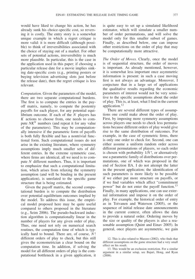
FIGURE 2Distribution of Movie’s Box Office Revenues over Its Life Cycle

0%

5%

10%

15%

20%

25%

30%

35%

40%

1 2 3 4 5 6 7 8 9 10 11+

Week from Release

Fra

ctio

n o

f E

ven

tual

Rev

enu

es

0%

10%

20%

30%

40%

50%

60%

70%

80%

90%

100%

Cu

mu

lati

ve R

even

ues

no weights

revenue weights

no weights(cumulative)

revenue weights(cumulative)

Notes: The “no weights” series calculates weekly percentages for each film separately, and then applies simple averagesof these percentages over all movies. The “revenue weights” series calculates a weighted average, where the weights areproportional to the total box office revenues of each movie. This figure shows the distribution of total box office revenuesover the movie’s life cycle. The bars stand for the week-by-week share, while the lines stand for the cumulative share as ofthe end of the corresponding week. It can be seen that most of the revenues are concentrated in the first few weeks, with thefirst week accounting, on average, for almost 40% of the eventual box office revenues, and the first four weeks accountingfor about 80% of them. Once I weight the averages by the gross box office revenues of the different films (white bars anddashed line), the distribution is less skewed and has a wider tail, suggesting that revenues of bigger movies decay slower.

more player-specific information and hence canuse this information to determine the order ofplay in a more natural way.

III. INDUSTRY AND DATA

The distributors of motion pictures are thosein charge of taking the movie from the end ofthe production stage to the theaters. This is donetypically by the distribution arm of the majorstudios, as described in more detail in Einav(2002) and in the references therein. One ofthe main strategic decisions made by distribu-tors is the movie release date. The two impor-tant considerations factored into this decisionare the strong seasonal effects in the demandfor movies and the competition that will beencountered throughout the movie’s run. Typi-cally, movies with higher expected revenues arereleased on higher demand weekends, so there isa trade-off between the seasonal and the com-petition effects. The importance of the releasedate is greatly magnified by the fact that theperformance during the first week accounts fora sizeable amount of the overall performance ofthe movie. On average, box office revenues in

the first week account for almost 40% of thetotal domestic revenues (Figure 2).14 An addi-tional reason for the importance of the releasedate choice is the view that high revenues inthe first week create information and networkeffects which increase revenues in subsequentweeks.15

Figure 3 presents the strong seasonality in theindustry, plotting weekly average industry rev-enues (normalized by ticket prices and the sizeof the U.S. population). Major holidays suchas Memorial Day, Fourth of July, Thanksgiv-ing, Christmas, and New Year’s are historicallyassociated with strong box office performance.Consistent with this revenue pattern, the con-ventional wisdom is that box office revenues arestrong throughout the summer season and duringthe Christmas winter holiday period. The periodfollowing Labor Day up to mid-November is

14. Furthermore, about 70% of the weekly revenues arecollected in the weekend.

15. To quote from Lukk (1997): “In this business, if youare not the number one film the week you are open, youusually are never the number one.” See also Moretti (2007)and Moul (2007).


FIGURE 3Seasonal Effects in Total Admissions

0

0.02

0.04

0.06

0.08

0.1

0.12

0.14

0.16

0.18

0.2

1 3 5 7 9 11 13 15 17 19 21 23 25 27 29 31 33 35 37 39 41 43 45 47 49 51 53 55

Week

Ave

rag

e In

du

stry

Sh

are

Labor Day

Thanksgiving

Xmas

PresidentDay

MemorialDay

Fourth ofJuly

Notes: This figure shows the seasonality in total industry sales. The vertical axis (“industry share”) is the industry’sweekly revenues, normalized by average ticket price and by the U.S. population. Thus, it can be thought of as the per capitanumber of movies seen each week (an industry share of, say, 0.1 implies that 1 of every 10 people in the United Statesgoes to the movies in the corresponding week). The figure shows the industry shares, averaged over the 1985–1999 sampleperiod. The figure clearly demonstrates the perceived seasonal effects in the industry. The year has two strong periods, thelong summer period (Memorial Day to Labor Day) and the Christmas Winter holiday period. The Spring and the Fall aretypically considered very weak periods for the industry, and the drop after Thanksgiving is generally seen as a “shoppingperiod.” The dashed lines stand for deviations of two standard errors. The number of weekly dummies is 56 to account forthe timing variation in U.S. holidays across the years (see Einav 2007 for details).

considered to be very weak, as is the period fromthe beginning of March to mid-May.

The identity of the competing movies is thesecond consideration taken into account whensetting the release date. Distributors are wary ofreleasing a movie in close proximity to anothermovie with which competition will be strong.Furthermore, even once release dates are set,distributors often change them in response tonew information concerning release dates ofsimilar movies chosen by other distributors (seein more detail later on). Another strategy prac-ticed by distributors is to announce their movie’srelease data early with the hope that preemp-tive action will deter other distributors fromchoosing the announced date. This practice isespecially common with movies that are widelyexpected to be successful.

I use two distinct data sets for this paper.The first contains detailed information about allmovies domestically released between 1985 and1999 and is described in detail in the compan-ion paper (Einav 2007). There I use these data to

obtain demand estimates. Some of the estimatesfrom the demand system are used in the cur-rent paper as an input into the empirical modelproposed above. To motivate the applicabilityof the empirical model described above to therelease date decision, I collected a second dataset. This is a unique data set regarding the prere-lease information about scheduled release dates,describing the dynamic process that leads to theeventual schedule. The source of the data is the“Feature Release Schedule,” which is publishedmonthly by Exhibitor Relations Inc.

In the beginning of each month, the publi-cation lists the updated release schedule of allmovies that are in the making but have not beenreleased as of yet. Typically, movies are firstlisted about 12–18 months before their sched-uled release. At this stage, many of the moviesare in the process of casting or are in earlystages of production. Thus, when first enter-ing the monthly report, movies are generallynot assigned to a specific release date. Rather,they are given a more general release season,


such as “Summer 2002,” “Christmas 2002,”or just as “coming.” As the scheduled releaseapproaches, the release date becomes more spe-cific, for example, “Late Summer 2002” or“Early July 2002,” converging eventually to aspecific date.16

The data cover roughly all the titles that wereeventually released between 1985 and 1999, atotal of 3,363 titles. To get an idea of what thedata look like, let me use Bruce Willis’s DieHard: With a Vengeance (aka Die Hard 3 ) asan example. It was first listed as “May 1995”in the September 1994 issue of the publication.In December 1994, the schedule became morespecific—May 12, 1995—but a month later itwas pushed back by two weeks, to May 26,1995 (Memorial Day). In February 1995, themovie’s release was moved again, to May 19,1995, which was the eventual release date. Thesequence of announcements for the 1999 releaseof Star Wars: The Phantom Menace was lesseventful; it was first listed as “May 1999” inthe issue of May 1998. In the September 1998issue, the announcement became more specific,May 21, 1999, and remained the same until itsactual release.17

A major characteristic of the data is the fre-quent changes in the release schedule of certainmovies. This is somewhat surprising, given thecosts associated with changing a release date.Such costs are incurred for several reasons, suchas committed advertising slots, the implicit costsof reoptimizing the advertising campaign, repu-tational costs, etc. The costs become higher asthe changes in release date are done closer to thescheduled release. While some of these changesare the result of unforeseen production delays,18

most of these changes are made for strategicreasons, and may provide some indication ofunobserved characteristics of the movie, suchas quality and commitment power. Supportingthis idea, industry practitioners and the popularmedia describe the scheduling game as a war ofattrition.

16. Agency issues provide an additional incentive forearly announcements of release dates. The director typicallyedits the film until the very last day before the release, sothe announced release date is used to set a final deadline tothe production process.

17. In fact, in the April 1999 issue, the May 21(Friday) announcement was changed to May 19 (Wednes-day). However, as will be discussed later, I tabulate datesat the weekly level, making these two dates effectivelyidentical.

18. See Einav and Ravid (2007) for analysis of suchschedule changes.

Across all movies and announcements, morethan 20% of the monthly announcements arechanges in relation to the most recent announce-ment of the same film. Moreover, more than60% of the movies changed their release dates atleast once. Figure 4 provides the distribution ofthe magnitude (in weeks) of these changes. Thedistribution of these changes is roughly sym-metric, and the majority of changes shift therelease date by a small number of weeks; 75%of the observed changes do not shift the releasedate by more than a month. Both the symme-try of the distribution and its shape indicate thatit is unlikely that the majority of changes aremade for exogenous nonstrategic reasons, suchas production delays. The likelihood of a moviechanging its release date is not significantly cor-related with the movie’s size, measured by itsproduction cost. However, movies with higherbox office quality (as estimated in Einav 2007)are significantly less likely to change releasedates. One interpretation of this is that movies’estimated quality is originally highly correlatedwith their production cost, but as the shape ofthe finished product becomes clearer, films thatturn out to be potential disappointments shiftaway from their previously announced releasedates.

This pattern of frequent small switches seemsconsistent with the idea that movies, in general,are produced with a target season in mind, whilethe “fine-tuned” choice of the precise releasedate within the season is subject to more strate-gic consideration. Because over 75% of themovies are released on Fridays, and an addi-tional 20% on Wednesdays, it seems naturalto think of the release decision as a discretechoice among a small number of alternatives.Such a pattern lends itself nicely to the empir-ical model described in the previous section:at the end of the production stage each movieis scheduled to release during a specific sea-son, while the exact release week is the out-come of a strategic timing game played againstall other movies released during the sameseason.

While the true timing game is probably bestapproximated by a repeated announcement gamewith increasing switching costs (see Caruanaand Einav 2008 for a formal analysis of suchgames), using such games for estimation iscomputationally infeasible. Therefore, the once-and-for-all sequential-move game, as proposed


FIGURE 4Distribution of the Magnitude of Switches in Announced Release Dates

0.00%

1.00%

2.00%

3.00%

4.00%

5.00%

tail

-17

-15

-13

-11 -9 -7 -5 -3 -1 1 3 5 7 9 11 13 15 17 ta

il

Magnitude of Switch (Weeks)

78.37%

Notes: This figure is based on 1,897 movies, covering movies that were eventually released nationwide between 1985and 1999. The figure shows the distribution of the magnitude of switches of announced release dates. A switch is a change inthe announced release date compared to the most recent announcement of the same movie (which is generally made a monthbefore). The distribution is taken over all movies and announcements, and tabulates the difference (in weeks) between thenew announcement and the previous one. A difference of 0 implies no change. A positive difference implies a shift forward ofthe release date, and a negative difference implies making the release date earlier than announced before. This figure providestwo main insights. First, the distribution is roughly symmetric (with a somewhat fatter tail in the positive part, for obviousreasons). Second, the majority of the changes shift the release date by a small number of weeks. These two observationssuggest that these changes are done mainly for strategic reasons, and not because of exogenous factors, such as productiondelays. Note that the bar at 0 is out of scale, and accounts for 78% of the announcements.

in Section II, may be viewed as a reasonablealternative.19

IV. SPECIFICATION AND RESULTS

A. Overview

In the companion paper (Einav 2007), I esti-mate demand for motion pictures, where theweekly demand for a movie is driven by threecomponents: the quality of the movie, the decayin quality since the movie’s release, and theunderlying seasonal pattern. Using a simplenested logit specification (with one nest for allmovies, and a second nest for the outside good),the weekly market share of movie j during week

19. One can think about the once-and-for-all assumptionas if switching costs are insignificant early on, but becomevery high at a certain point in time. The order of movesassumed for the sequential game is just the ordering of thepoints in time at which these jumps in the switching costsoccur.

t is given by

sjt = (Dσt + Dt)

−1 exp((θj − λ(t − rj )

+ τt + ξjt)/(1 − σ)),(11)

where θj is the movie quality,20 rj is therelease date (in weeks) of movie j, τt is theunderlying level of demand in week t, ξjt isa disturbance term which reflects the deviationfrom the common decay pattern, Dt is given by

Dt =∑k∈Jt

exp((θk − λ(t − rk)

+ τt + ξkt)/(1 − σ)),(12)

and Jt is the set of movies in theaters duringweek t. An important finding of Einav (2007)is that the estimates for underlying seasonality

20. One should think of quality as reflecting attractive-ness or “box office appeal,” which is not necessarily relatedto cinematographic quality.


FIGURE 5Seasonal Effects in Underlying Demand

-1

-0.6

-0.2

0.2

0.6

1

1 3 5 7 9 11 13 15 17 19 21 23 25 27 29 31 33 35 37 39 41 43 45 47 49 51 53 55

Calendar Week

Est

imat

ed c

oef

fici

ent

Labor Day

Thanksgiving

Xmas

PresidentsDay

MemorialDay

Fourth ofJuly

Notes: This figure plots the estimated coefficients on the weekly dummy variables from estimating the nested logit moviedemand model of Einav (2007). There are two major differences compared to the seasonal pattern of industry revenues(Figure 3). First, the seasonal variation is smaller, suggesting that about one-third of the seasonal variation is explained byvariation in quality. Second, the seasonal pattern is slightly different, with, for example, the end of the summer lookingrelatively much better than industry revenues indicate. The dashed lines stand for deviations of two standard errors. Theestimated decay coefficient λ is −0.22 (with a standard error of 0.014) and the estimated substitution coefficient σ is 0.524(0.030). The number of observations is 16,103 (1,956 movies). The number of weekly dummies is 56 to account for thetiming variation in U.S. holidays across the years (see Einav 2007 for details).

are somewhat different from the conventionalwisdom, as reflected by Figure 3. I reproducethese estimates for underlying seasonality inFigure 5.

Simple analysis may suggest that, taking theestimates for underlying seasonality as given,distributors do not make their release deci-sions according to these estimates. The seasonalrelease pattern is described in Figure 6, showingthat many of the top movies are released on afew big holiday weekends. The current applica-tion complements these findings by addressingtwo key issues. First, it examines the within-season variation in the release pattern, address-ing a concern that the choice of a season maybe driven by other omitted factors.21 Second, itaccounts for strategic effects by using the empir-ical model developed in this paper.

21. For example, many movies may release early inthe summer in an attempt to leave enough time to makethe high-demand video and DVD season around Christmas.Certain movies may also cater to a specific target audience,and characteristics of moviegoers change across seasons. Allthese factors are less relevant when considering the choiceof a specific week within a given season.

The estimation strategy is to take the demandestimates of movie quality and decay pattern asgiven, and to estimate the underlying demandparameters from the game, that is, from theobserved release pattern. The focus on theunderlying demand is for several reasons. First,the other parameters of the demand system areless controversial, and hence make it a less inter-esting exercise. Second, the estimates of under-lying seasonality from the demand system aremore sensitive to the identification assumptionemployed in Einav (2007), that the unobserv-able component of the decay is independent ofthe choice of release date. Therefore, it may beuseful to search for alternative sources of infor-mation about these parameters. Finally, a simpleinspection of the results from the demand esti-mation suggests that distributors have a differentseasonal pattern in mind when deciding aboutrelease dates compared to the seasonal patternestimated. This calls for a more formal treat-ment, which would establish and quantify thispattern more analytically.

More generally, one may think about thisapplication in the context of standard demand


FIGURE 6Seasonal Effects in New Releases

0

1

2

3

4

5

6

7

8

9

10

1 3 5 7 9 11 13 15 17 19 21 23 25 27 29 31 33 35 37 39 41 43 45 47 49 51 53 55

Calendar Week

"New

Rel

ease

Eff

ect"

LaborDay

Thanksgiving

Xmas

Presidents Day

Memorial Day

Fourth of July

Notes: This figure plots the estimated release effect, which is defined as the contribution of new movies to the competitioneffect (see Einav 2007 for more details). It is then averaged over the 15 years of the data. The dashed lines stand for twostandard errors from the average (ignoring the implicit standard error that comes from coefficient uncertainty). The numberof weekly dummies is 56 to account for the timing variation in U.S. holidays across the years (see Einav 2007 for details).

estimation. One strategy is to estimate a demandsystem combined with assumptions on the gameplayed among firms. This approach is efficient,provided that the assumptions regarding firms’behavior are correct. It provides inconsistentestimates, however, if these assumptions areincorrect. This approach does not allow us totest for the optimality of firm behavior, as itis assumed. A second strategy is to estimatedemand parameters from demand data alone,and then use these estimates to test the optimal-ity of firms’ behavior. This is the approach takenin this paper for two main reasons. First, it iscomputationally not feasible to estimate movie-specific qualities as parameters of the timinggame; these qualities enter nonlinearly, requiringa numerical search procedure over many param-eters. Second, the underlying demand parame-ters obtained from the demand system are quitedifferent from industry wisdom, questioning theplausibility of pooling demand- and supply-sidemoments. Instead, I find it more informative toobtain these set of estimates separately and com-pare them.

Consequently, the seasonal estimates result-ing from estimating the timing game should be

thought of as the perceived underlying demand,that is, the underlying demand that rational-izes the observed release pattern. The interestingexercise is to compare these estimates to thosederived from the demand system. As it turnsout, these two sets of estimates of underlyingdemand are quite different. While I view thisas some indication for bounded rationality ofdistributors (see later), it is perfectly consistentwith the reverse interpretation: if one believesthat the timing game is specified correctly andthat distributors are fully rational, then the dif-ferent patterns call into question the validity ofthe identification assumption used to obtain thedemand estimates.

B. Specification

The general setup for the estimation is asfollows. I choose several time windows (“sea-sons”) within the year and take the set ofmovies that were released within the speci-fied season as given. I then analyze the choiceof the week within the season during whichthe movie is released. The motivation for thisassumption comes from the prerelease timing


data described in Section III. Distributors decidefar in advance that a certain movie is scheduledfor around, say, Memorial Day, but only laterdecide about the specific date on which it isreleased. Moreover, most changes of previouslyannounced release dates do not shift the date bymuch.

The empirical model developed in Section IIprovides the framework for analysis. For themodel to be taken to the data, I still need to spec-ify the particular functions and the model param-eters. In doing so, I am guided by two mainconsiderations. First, the computational burdendictates a restricted choice of K (the numberof weeks included in each season) and N (thenumber of strategic players), and a relativelysmall number of parameters. This is done bysetting the length of each season to 5 weeks(K = 5), a choice which is guided by the switch-ing behavior described in Figure 4. I let N beequal to 2–6, depending on the specificationand the number of parameters estimated. I alsoestimate only a small number of parameters.As mentioned, the second important consider-ation for specifying the functional forms is myattempt to evaluate the timing decisions madeby distributors.

I assume that each season represents anindependent timing game. In each season, eachof the N players (those that eventually releasedtheir movie during that season) chooses one of Kweeks (that lie within the season) during whichhis movie is released. Movies are generallyreleased on Fridays, consistent with analyzingthe timing decision at the weekly level. Tofurther reduce the dimensionality problem, Ichoose to model only the best N movies withinthe season as strategic players. The qualitymeasure of each movie is given by the pointestimate of the movie fixed-effect estimated inEinav (2007). I assume that these movies playagainst each other, conditioning on the observedrelease dates of all other movies.22

22. A reasonable approach would be to assume that theorder of moves is dictated by the ordering of the moviequalities, the biggest movie playing first. This implies thatthe smallest movies condition their decisions on the releasedates of the bigger ones, but not vice versa (which is whatI do in this paper). Given the computational restrictions,such an approach would rely on the decisions of the small,less strategic, players. For these movies, it is not clear thatwe need the “high-powered” structural game for estimation.Rather, given that they have no real strategic effect, we canestimate each movie’s decision separately.

Given that all movies remain in the mar-ket for longer than one week, not only dothe “active” players (top quality movies) con-dition on the release pattern of the lower qualitymovies within the season, but they also condi-tion on the release pattern of all movies in adja-cent seasons. While conditioning on the releasedates of movies from the preceding season issensible, it is questionable whether it is validto assume that movies can condition on therelease dates of movies in the subsequent sea-son. I justify this assumption by the fast decayof box office revenues, which implies that theeffect of movies that are released more thanone week apart is relatively small, and hencehas little effect on strategic considerations. I usethese other movies and their observed releasedates to calculate the counterfactual box officerevenues.

For estimation, I choose four annual releaseseasons, which are all centered around a dom-inant release date. These are Presidents’ Day,Memorial Day, Fourth of July, and Thanks-giving.23 Each season includes the dominantweek, and 2 weeks before and after, adding upto 5 weeks in each season (i.e.,K = 5, as spec-ified earlier). Thus, I use a total of 60 seasons(four seasons over 15 years), on which the esti-mates are based. The number of movies in eachseason is between 6 and 17 with a mean of11.2 and standard deviation of 2.34, but moviequality is very skewed. For example, the esti-mated quality of the top three movies accountsfor 44–91% (with a mean of 66%), as a fractionof the total quality of all movies in the season.Thus, restricting attention to only the top moviesaccounts for the majority of the industry boxoffice revenues in the season in which they arereleased.

As explained in the previous section, Ikeep the nested logit specification, which wasthe basis for the demand analysis in Einav(2007), and use the point estimates from thedemand system, but free up some parameters.Specifically, I assume that the known portion of

23. Christmas, a highly popular release date, is not usedfor the analysis for two reasons. First, the timing of manyChristmas releases is driven by Academy Award eligibilityrequirements rather than by strategic motives. Second, unlikethe other seasons, Christmas is not characterized by a singlepopular release date; the entire second half of December ispopular among moviegoers.


TABLE 1Estimation Results, Pooling All Seasons

A. Assuming better movie moves first

Number of strategicmovies (N ) 3 4 5 3 4 5

η 1.13 (0.66) 1.14 (0.63) 1.12 (0.60) 1.18 (0.68) 1.20 (0.64) 1.18 (0.61)α 1.72 (2.42) 2.12 (2.23) 2.03 (2.17)Log likelihood −283.3 −378.0 −472.9 −283.3 −377.9 −472.8

B. Assuming random (uniform) order of moves

Number of strategicmovies (N ) 3 4 5 3 4 5

η 0.28 (1.13) 0.31 (1.18) 0.70 (1.38) 1.58 (1.24) 1.86 (1.38) 2.82 (1.70)α 23.51 (16.52) 21.37 (14.40) 23.24 (16.31)Log likelihood −284.8 −379.8 −474.7 −284.0 −378.9 −473.3

Notes: The table presents the results from a set of specifications of the timing game. Panel A takes the order of movesas given, with the better movie moving first, while Panel B assumes a uniform distribution over all order permutations.Standard errors in parentheses. For comparison, note that the log likelihood of a fully random release date choice (i.e., η = 0)is 60 · ln(5−N).

distributors’ profits takes the following form:

πj (rj , r−j ; γ) =rj +H∑t=rj

sjt(rj , r−j ; α, σ)

=rj +H∑t=rj

(Dσt + Dt )

−1

exp((θj−λ(t−rj )+ατt )/(1−σ)),(13)

[Equation amended after online publication dateSeptember 29, 2009.]where

Dt =∑

k∈Jt (rj ,r−j )

exp((θk − λ(t − rk)

+ ατt)/(1 − σ)),(14)

and θj is the estimated quality of the movie,λ is the estimated decay parameter, rj is the(endogenous) movie’s release decision, and τt

is the estimated underlying demand. H is thelength of the period that is taken into account bydistributors when making their release decision.The choice of H is guided by computational lim-itations, so I choose H = 2, thereby restrictingdistributors to base their decisions on the firstthree weeks after the release. Jt (rj , r−j ) is theset of movies that play on week t, which dependson the observed release dates of the nonstrategicmovies as well as on the (endogenous) release

decisions, rj and r−j , of the strategic movieswhich are being modeled.

That is, I use Equation (11) with small mod-ifications. First, I assume that distributors maketheir decisions under the assumption that ξj t =0 for any j and t.24 Second, while all the param-eters in the profit function are taken as given(based on the demand estimates), I introduce anew parameter, α. In the nested logit demandsystem, this parameter is restricted to be 1.Freeing it up allows distributors to overweight(α > 1) or underweight (α < 1) the estimatedunderlying demand.

Finally, an additional parameter to be esti-mated in all specifications is η, the precision ofthe logit error term as described in Section II.It does not show up in Equation (13) because itaffects π = π + ε only through the error term,but not through π. The results reported belowalso use different assumptions regarding theorder of moves (see Section II).

C. Results

Table 1 present the estimation results for dif-ferent choices of N, the number of strategicmovies. Panel A presents results that are based

24. One could think of imputing ξj t from the demandsystem, and assuming that the ξj t ’s are related to the movie-specific decay pattern. Doing so changes the results verylittle. This is because the variation of ξj t ’s is very smalland hence has little effect on the strategic considerations.


on an order of moves (of the sequential game)where the better movie moves first, while panelB present results where I allow a uniform dis-tribution over all orders (permutations of the Nplayers). Although the qualitative results (dis-cussed below) are similar across both panels,the random order leads to somewhat less sta-ble results and lower statistical significance ofthe coefficients, so I focus my discussion on theresults of panel A, which constitutes my pre-ferred specification.

Overall, the results are quite stable across dif-ferent choices of N. In all specifications, theestimate of η is positive and significant at a10% confidence level. Recall that η is the pre-cision of the error term. Alternatively, one canalso think of η as the parameter on the deter-ministic component of payoffs. An insignificantη would imply that the release date decisionsappear random with respect to the modeled pay-offs, and a negative η would imply that themodeled payoffs are negatively associated withthe release date decision. Therefore, the positiveand (marginally) significant estimate of η sug-gests that the model for payoffs, together withthe estimated demand parameters, is indeed use-ful in explaining the release date decisions.

Perhaps more interesting is the estimate of α.Across all specification, the point estimates of αare consistently above 1, which is the impliedvalue of the nested logit demand system.25

This suggests that movie distributors overweightunderlying seasonality (relative to competitionfrom other movies) when they make their releasedate decision. In other words, to best rationalizethe observed release date decision, the estimatedunderlying demand estimates need to be aboutdoubled; that is, the spike of underlying demandin, say, Memorial Day weekend needs to betwice as large to rationalize the clustering of hitmovies released on that weekend.

Thus, the results taken together suggest thatalthough distributors tend to respond to under-lying demand and to competition from othermovies, as implied by the demand model, theyappear to be too clustered in holiday weekends.To make this statement more precise, and toprovide more interpretable figures, I construct

25. None of the estimates of α is significantly differentfrom 1 (or from 0) at reasonable confidence levels. This maynot be surprising given the small number of independentseasons (60) used for estimation, which makes standarderrors large. However, given the fairly stable estimate ofα across choices of N, interpreting and discussing the pointestimates may not be unreasonable.

a measure for clustering. In a given season, fora given choice of N, I define the clustering mea-sure as the average fraction of quality releasedon the holiday weekend. Let θi

m be the qualityof movie i, which is released in season m, so theaverage clustering measure across M markets isgiven by

clustering = 1

M

m=M∑m=1

( ∑ri is holiday

θim

)/(∑i

θim

).

(15)

This is the actual clustering measure. I con-struct the corresponding counterfactual by usingthe expected clustering measure, where theexpectation is taken over the idiosyncratic noisein the empirical model, and over the distributionof the permutations of order of play. One shouldnote that the clustering measure is between 0 and1, and that with K = 5, a random assignmentof movies into release dates yields a clusteringmeasure of K−1 = 0.2.

Across all seasons and years, the averageclustering measure ranges from 0.35 to 0.37(across choices of N ) compared to the randomassignment measure of 0.2. Computing expectedclustering measures using the point estimatesfrom the various specifications of Table 1 thatimpose a value of α = 1, I obtain measuresthat range from 0.16 to 0.25. That is, thenested logit demand model implies a muchmore even distribution of movie quality withina season, requiring overweighting of underlyingseasonality to rationalize the much higher actualclustering observed in the data.

Table 2 presents some results when eachrelease season is estimated separately. I am hes-itant to experiment much with various specifi-cations because each such specification relieson only 15 independent seasons. Table 2 is stillinstructive in showing that pooling together allseasons may hide important heterogeneity. Specif-ically, the results presented in Table 2 show thatthe model does a pretty good job in explain-ing release date decisions in the summer (i.e.,around Memorial Day and Fourth of July),while the release date decisions around Thanks-giving, and even more so around Presidents’Day, are hardly associated with expected prof-its, as modeled and estimated by the demandsystem.

D. Discussion

The main conclusion from the empirical anal-ysis of this paper is that distributors seem


TABLE 2Estimation Results, by Season

Number of strategicmovies (N ) 2 3 4 5 6

Presidents’ Dayη 0.00 (0.01) 0.08 (1.41) 0.07 (1.36) 0.00 (0.0) 0.00 (0.01)Log likelihood −45.1 −67.6 −90.1 −112.7 −135.2

Memorial Dayη 2.20 (1.25) 2.08 (1.18) 1.79 (1.19) 1.90 (1.16) 1.98 (1.19)Log likelihood −46.6 −70.8 −95.3 −119.1 −143.2

Fourth of Julyη 0.00 (0.04) 1.87 (1.80) 1.94 (1.66) 2.34 (1.46) 1.74 (1.40)Log likelihood −48.3 −71.8 −95.7 −119.1 −143.9

Thanksgivingη 0.23 (1.41) 0.49 (1.17) 0.83 (1.05) 0.56 (1.04) 0.55 (0.97)Log likelihood −48.3 −72.3 −96.2 −120.6 −144.7

Notes: The table presents the results from a set of specifications of the timing game, separately by season. All results takethe order of moves as given, with the better movie moving first (as in panel A of Table 1). Standard errors in parentheses. Forcomparison, note that the log likelihood of a fully random release date choice (i.e., η = 0) is 15· ln(5−N). Note that almostno estimate is statistically significant at reasonable confidence levels. This is mainly due to the small number of observationsonce each season is allowed to have its own parameters.

to cluster their release dates more than theyshould. While the spirit of the results is some-what similar to the conclusions drawn in Einav(2007), the results in the current paper arelargely driven by different variation in the data.Einav (2007) uses cross-seasonal variation and“price-taking” assumptions, while here I usewithin-season variation and allow for strate-gic effects. Thus, at least a priori, there wasno reason to assume that the two analyseswould yield similar qualitative results. The factthat they do, therefore, strengthens these con-clusions. In what follows, I propose severalexplanations that may help understand thesefindings.

The first line of interpretations is consistentwith the assumptions of optimizing behavior bystudios. There are several industry features, notincorporated in my model, that could cause moremovie clustering around high-demand weekendsthan predicted by the model. First, uncertaintymay play an important role. While a completeinformation equilibrium may have the moviesspreading out over the different weeks, uncer-tainty may result in more movies being releasedon the better weeks. This over-clustering mayprove inefficient ex-post, but may be optimalex-ante. To gain intuition for why this may bethe case, consider a two-by-two game in whichthe ex-post profits are given by

Holiday Non-HolidayHoliday 100, 0 100, 40Non-Holiday 40, 100 10, 0

where the motivating story is that the marketsize is 100 and 40 in the holiday and non-holidayweeks, respectively. Movie 1 (the row player)always obtains the whole market, independentlyof competition, while movie 2 makes positiverevenues only if movie 1 is not present. Theequilibrium of this model is for movie 1 torelease on the holiday weekend, and for movie2 to release on the non-holiday weekend, thatis, no clustering. Consider now an extremeuncertainty, in which both movies are identicalex-ante, and with probability 0.5 each moviewins the whole market if the two compete head-to-head. The new (ex-ante) payoff matrix wouldbe as follows:

Holiday Non-HolidayHoliday 50, 50 100, 40Non-Holiday 40, 100 10, 20

yielding a unique Nash equilibrium in whichboth movies are released on the holiday weekend,that is, clustering. Trying to allow uncertainty inthe empirical model is conceptually possible butcomputationally very intensive.


One can also rationalize the overclusteringresult by having the true value of a holidayrelease being greater than what we think it is.For example, this may be due to repeated gameeffects (Chisholm 1999), which may change thestatic “value” of releasing on a certain week.If a distributor who releases a movie on, say,the Fourth of July is more likely to capture thesame week in future years, a Fourth of Julyrelease may be more attractive than it is esti-mated to be. Alternatively, if there are nonmon-etary benefits (e.g., prestige) to the distributor(or to the director and the actors) from releas-ing on holiday weekends, this may also generateoverclustering effects.26 Third, as is well known,the nested logit specification used to obtain thedemand estimates assumes that all movies areequally good substitutes of each other, propor-tional to their market shares. If the top moviesevery season are of different genres, the rev-enues of these movies may be less affected byclustering with other movies.

A very different line of explanation is abehavioral one. Movie distributors could beoverconfident as to the relative quality of theirmovie (Camerer and Lovallo 1999) or couldsimply err in their assessment of the underlyingdemand in the industry. After all, the “learningfrom experience” argument, according to whicheconomic agents cannot err for a long period,may not work in the motion picture industry.To learn from experience, distributors have tofirst obtain enough experience and then be ableto use it properly. In particular, the informa-tion about the seasonal pattern comes only oncea year, and the high uncertainty about moviequality makes inference difficult regarding theseparation between the underlying demand andthe movie quality effects. With each movie hav-ing its own identity, a controlled experimentof releasing the same (or very similar) moviein different dates is not feasible. For decades,the industry has followed the same release pat-tern, according to which big hits are released onbig weekends. Thus, there are no natural exper-iments that make it easy to distinguish betweenhigher movie quality and higher underlyingdemand. Any deviation from the “predicted”seasonal pattern (for example, successful moviesin October) is typically interpreted by industryobservers as an extremely good movie in the

26. Consistent with this idea is the sentence I often heardwhile interviewing industry executives: “Economics? Thisindustry is not about economics; it is all about egos. . . .”

wrong season rather than as a decent moviein a mediocre season. In other words, thereis very little bad feedback after a bad releasedecision.

Even if distributors are fully rational, conser-vatism may lead them to stick to the traditionalrelease pattern. This conservatism may be mag-nified if we think of the institutional contextand the potential agency costs in the indus-try. Top directors and actors do not want tosee their films fail because of a poor market-ing decision. Thus, considering the traditionalrelease pattern in the industry, they frequentlylobby for a traditionally good choice of releasedates. Distributors are likely to be conservativeand satisfy these requests, rather than risk theirjobs, reputation, and future business. By stick-ing to the traditional release pattern they canbe adequately evaluated by the market.27 Thisis not the only example where the motion pic-ture industry seems to be conservative and tofollow tradition. Other examples include the cur-rent uniform ticket pricing policy in the industry(Orbach and Einav 2007), the use of stars in theindustry (Ravid 1999), or the massive capacityexpansion that took place in the 1990s and hasrecently led many of the largest chains of movietheaters to file for bankruptcy (Davis 2006a).

Finally, it should be noted that in recent yearsdistributors started to experiment more with lesstraditional release decisions. After relative suc-cessful early May openings of Gladiator andThe Mummy Returns in 2000 and 2001, the dis-tributors of Spiderman —an anticipated block-buster much before its actual release—decidedto release it on May 3, 2002. Ten years earliersuch a move would have been unheard of.

V. CONCLUSIONS

This paper develops a new empirical modelof discrete games to study the release date tim-ing game played by movie distributors. Thetiming game is formulated as a sequentialgame with private information, with distributorschoosing among a small set of release week-ends. The main empirical finding is that moviedistributors overcluster their release dates, withtoo many good movies released on big holidayweekends. As a whole, the results complementand strengthen similar (though weaker) conclu-sions found in Einav (2007).

27. This is in the spirit of “you cannot be fired for buyingIBM.” For a formal treatment, see Zweibel (1995).


In analyzing the timing game, the assumptionis that by the time the release date is chosen,many of the characteristics of the movie andof competing movies are already set, generatingheterogeneity among competitors. This provideseach player with a payoff-relevant identity.Accounting for this feature using existing mod-els of discrete games is difficult. This papertherefore proposes a new estimable game struc-ture that tries to relax this limitation. The modelspecifies a sequential game structure with asym-metric information. The game has a unique equi-librium that can be solved using a simple algo-rithm. This allows estimating a game even in theabsence of symmetry restrictions on the payoffstructure.

This last feature is crucial for a large set ofapplications. In particular, such flexibility wouldbe a necessary property of an empirical modelof discrete games that attempts to model loca-tion choice together with a state-of-the-art modelof price-setting behavior. As the demand litera-ture in industrial organization keeps going in thedirection of more flexible substitution patterns,one has to use product choice models that allowfor a more flexible functional form for payoffs.Combining these two literatures is an impor-tant direction for future research. The empiricalmodel proposed in this paper is a way that mayfacilitate such work.

REFERENCES

Aguirregabiria, V., and P. Mira. “Sequential Simulated-Based Estimation of Dynamic Discrete Games.”Econometrica, 75, 2007, 1–53.

Andrews, D., S. Berry, and P. Jia. “Confidence Regionsfor Parameters in Discrete Games with MultipleEquilibria, with an Application to Discount StoreLocations.” Manuscript, Yale University, 2007.

Bajari, P., C. L. Benkard, and J. Levin. “Estimating DynamicModels of Imperfect Competition.” Econometrica, 75,2007, 1331–70.

Bajari, P., H. Hong, and S. Ryan. “Identification and Esti-mation of a Discrete Game of Complete Information.”Manuscript, University of Minnesota, 2008.

Beresteanu, A., I. Molchanov, and F. Molinari. “SharpIdentification Regions in Games.” Manuscript, DukeUniversity, 2008.

Berry, S. “Estimation of a Model of Entry in the AirlineIndustry.” Econometrica, 60, 1992, 889–917.

Berry, S., J. Levinsohn, and A. Pakes. “Automobile Pricesin Market Equilibrium.” Econometrica, 63, 1995,841–90.

Berry, S., and J. Waldfogel. “Free Entry and SocialInefficiency in Radio Broadcasting.” RAND Journalof Economics, 30, 1999, 397–420.

Borenstein, S., and J. Netz. “Why Do All the FlightsLeave at 8 a.m.? Competition and Departure-TimeDifferentiation in Airline Markets.” InternationalJournal of Industrial Organization, 17, 1999, 611–40.

Bresnahan, T., and P. C. Reiss. “Entry into Monopoly Mar-kets.” Review of Economic Studies, 57, 1990, 531–53.

Camerer, C., and D. Lovallo. “Overconfidence and ExcessEntry: An Experimental Approach.” AmericanEconomic Review, 89, 1999, 306–18.

Caruana, G., and L. Einav. “A Theory of EndogenousCommitment.” Review of Economic Studies, 75, 2008,99–116.

Chisholm, D. C. “The War of Attrition and Optimal Timingof Motion-Picture Releases.” Manuscript, SuffolkUniversity, 1999.

Ciliberto, F., and E. Tamer. “Market Structure and Mul-tiple Equilibria in Airline Markets.” Manuscript,Northwestern University, 2008.

Corts, K. S. “The Strategic Effects of Vertical Market Struc-ture: Common Agency and Divisionalization in theU.S. Motion Picture Industry.” Journal of Economicsand Management Strategy, 10, 2001, 509–28.

Davis, P. J. “Measuring the Business Stealing, Cannibal-ization, and Market Expansion Effects of Entry in theU.S. Motion Picture Exhibition Market.” Journal ofIndustrial Economics, 54, 2006a, 293–321.

Davis, P. J. “Estimation of Quantity Games in the Presenceof Indivisibilities and Heterogeneous Firms.” Journalof Econometrics, 134, 2006b, 187–214.

Draganska, M., S. Misra, V. Aguirregabiria, P. Bajari,L. Einav, P. Ellickson, D. Horsky, et al. “DiscreteChoice Models of Firms’ Strategic Decisions.”Marketing Letters, 19, 2008, 399–416.

Einav, L. “Seasonality and Competition in Time: AnEmpirical Analysis of Release Date Decisions in theU.S. Motion Picture Industry.” Ph.D. dissertation,Harvard University, 2002.

Einav, L. “Seasonality in the U.S. Motion Picture Industry.”RAND Journal of Economics, 38, 2007, 127–45.

Einav, L., and A. Nevo. “Empirical Models of Imper-fect Competition: A Discussion,” in Advances inEconomics and Econometrics: Theory and Applica-tions, Vol. II, Chapter 3, edited by R. Blundell, W.K. Newey, and T. Persson. Ninth World Congress.Cambridge: Cambridge University Press, 2006, 86–96.

Einav, L., and A. Ravid. “Stock Market Response toChanges in Movies’ Opening Dates.” Manuscript,Stanford University, 2007.

Ellickson, P. B., and S. Misra. “Enriching Interactions:Incorporating Revenue and Cost Data into Static Dis-crete Games.” Manuscript, University of Rochester,2007.

Goettler, R. L., and R. Shachar. “Spatial Competition inthe Network Television Industry.” RAND Journal ofEconomics, 32, 2001, 624–56.

Lukk, T. Movie Marketing: Opening the Picture and GivingIt Legs. Los Angeles: Silman-James Press, 1997.

Mazzeo, M. J. “Product Choice and Oligopoly Market Struc-ture.” RAND Journal of Economics, 33, 2002, 1–22.

McKelvey, R. D., and T. R. Palfrey. “Quantal ResponseEquilibria in Extensive Form Games.” ExperimentalEconomics, 1, 1998, 1–41.

Moretti, E. “Social Learning and Peer Effects in Consump-tion: Evidence from Movie Sales.” NBER WorkingPaper No. 13832, 2007.

Moul, C. C. “Measuring Word of Mouth’s Impact onTheatrical Movie Admissions.” Journal of Economicsand Management Strategy, 16, 2007, 859–92.

Nevo, A. “Measuring Market Power in The Ready-to-EatCereal Industry.” Econometrica, 69, 2001, 307–42.

Orbach, B. Y., and L. Einav. “Uniform Prices for Differenti-ated Goods: The Case of the Movie-Theater Industry.”International Review of Law and Economics, 27, 2007,129–53.


Orhun, Y. “Spatial Differentiation in the SupermarketIndustry.” Manuscript, UC Berkeley, 2005.

Pakes, A., M. Ostrovsky, and S. Berry. “Simple Estimatorsfor the Parameters of Discrete Dynamic Games, withEntry/Exit Examples.” RAND Journal of Economics,38, 2007, 373–99.

Quint, D., and L. Einav. “Efficient Entry.” EconomicsLetters, 88, 2005, 278–83.

Ravid, S. A. “Information, Blockbusters, and Stars: AStudy of the Film Industry.” Journal of Business, 72,1999, 463–92.

Reiss, P. C. “Empirical Models of Discrete StrategicChoices.” American Economic Review Papers andProceedings, 86, 1996, 421–26.

Seim, K. “An Empirical Model of Firm Entry withEndogenous Product-Type Choices.” RAND Journalof Economics, 37, 2006, 619–40.

Simonsohn, U. “eBay’s Crowded Evenings: CompetitionNeglect in the Field.” Manuscript, UC San Diego,2008.

Sweeting, A. “The Strategic Timing of Radio Commercials:An Empirical Analysis Using Multiple Equilibria.”Manuscript, Duke University, 2008.

Tamer, E. “Incomplete Simultaneous Discrete ResponseModel with Multiple Equilibria.” Review of EconomicStudies, 70, 2003, 147–65.

Toivanen, O., and M. Waterson. “Market Structureand Entry: Where’s the Beef?” RAND Journal ofEconomics, 36, 2005, 680–99.

Watson, R. “Product Variety and Competition in theRetail Market for Eyeglasses.” Journal of IndustrialEconomics, 57(2), June 2009, 217–251.

Zweibel, J. “Corporate Conservatism and Relative Compens-ation.” Journal of Political Economy, 103, 1995, 1–25.

NOT ALL RIVALS LOOK ALIKE: ESTIMATING AN EQUILIBRIUM MODEL ...leinav/pubs/EI2010.pdf · NOT ALL...

Documents

Transcript of NOT ALL RIVALS LOOK ALIKE: ESTIMATING AN EQUILIBRIUM MODEL ...leinav/pubs/EI2010.pdf · NOT ALL...